the mathematics of credit derivatives: firm’s value...
TRANSCRIPT
The Mathematics of Credit Derivatives:Firm’s Value Models
Philipp J. Schonbucher
London, February 2003

➠ ➡➡ ➠ ■ ? WBS Training: Unit 4 (c) Philipp J. Schonbucher
Basic Idea
Black and Scholes (1973) and Merton (1974):
Shares and bonds are derivatives on the firm’s assets.
Limited liability gives shareholders the option to abandon the firm, to put it to thebondholders.
Bondholders have a short position in this put option.
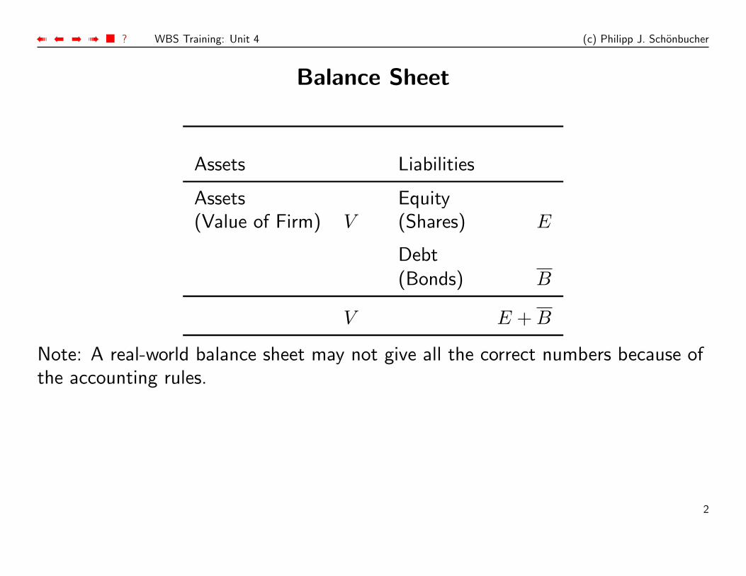
Accounting identity:
Assets = Equity + Liabilities
V = E + B
1
➠ ➡➡ ➠ ■ ? WBS Training: Unit 4 (c) Philipp J. Schonbucher
Balance Sheet
Assets Liabilities
Assets Equity(Value of Firm) V (Shares) E
Debt(Bonds) B
V E + B
Note: A real-world balance sheet may not give all the correct numbers because ofthe accounting rules.
2
➠ ➡➡ ➠ ■ ? WBS Training: Unit 4 (c) Philipp J. Schonbucher
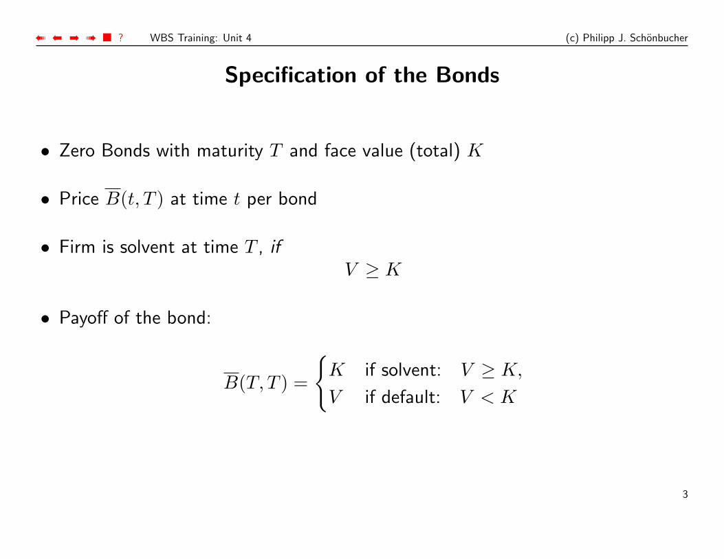
Specification of the Bonds
• Zero Bonds with maturity T and face value (total) K
• Price B(t, T ) at time t per bond
• Firm is solvent at time T , ifV ≥ K
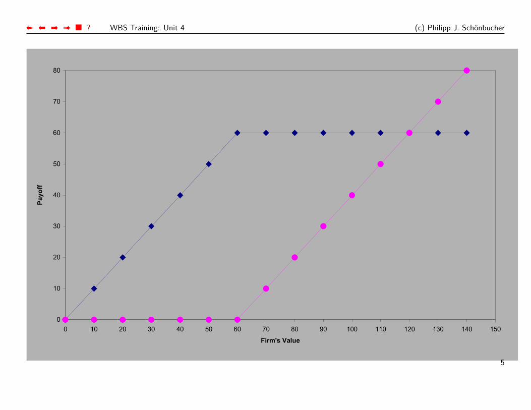
• Payoff of the bond:
B(T, T ) =
{K if solvent: V ≥ K,
V if default: V < K
3
➠ ➡➡ ➠ ■ ? WBS Training: Unit 4 (c) Philipp J. Schonbucher
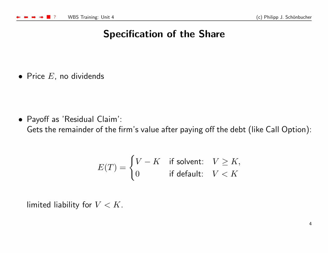
Specification of the Share
• Price E, no dividends
• Payoff as ’Residual Claim’:Gets the remainder of the firm’s value after paying off the debt (like Call Option):
E(T ) =
{V −K if solvent: V ≥ K,
0 if default: V < K
limited liability for V < K.
4
➠ ➡➡ ➠ ■ ? WBS Training: Unit 4 (c) Philipp J. Schonbucher
5
➠ ➡➡ ➠ ■ ? WBS Training: Unit 4 (c) Philipp J. Schonbucher
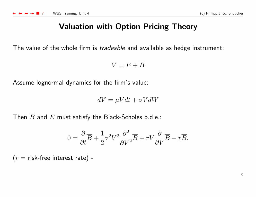
Valuation with Option Pricing Theory
The value of the whole firm is tradeable and available as hedge instrument:
V = E + B
Assume lognormal dynamics for the firm’s value:
dV = µV dt + σV dW
Then B and E must satisfy the Black-Scholes p.d.e.:
0 =∂
∂tB +
12σ2V 2 ∂2
∂V 2B + rV∂
∂VB − rB.
(r = risk-free interest rate) -
6
➠ ➡➡ ➠ ■ ? WBS Training: Unit 4 (c) Philipp J. Schonbucher
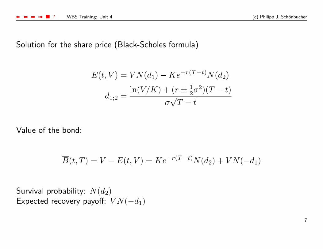
Solution for the share price (Black-Scholes formula)
E(t, V ) = V N(d1)−Ke−r(T−t)N(d2)
d1;2 =ln(V/K) + (r ± 1
2σ2)(T − t)
σ√
T − t
Value of the bond:
B(t, T ) = V − E(t, V ) = Ke−r(T−t)N(d2) + V N(−d1)
Survival probability: N(d2)Expected recovery payoff: V N(−d1)
7
➠ ➡➡ ➠ ■ ? WBS Training: Unit 4 (c) Philipp J. Schonbucher
8
➠ ➡➡ ➠ ■ ? WBS Training: Unit 4 (c) Philipp J. Schonbucher
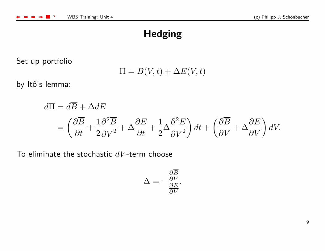
Hedging
Set up portfolioΠ = B(V, t) + ∆E(V, t)
by Ito’s lemma:
dΠ = dB + ∆dE
=(
∂B
∂t+
12∂2B
∂V 2 + ∆∂E
∂t+
12∆
∂2E
∂V 2
)dt +
(∂B
∂V+ ∆
∂E
∂V
)dV.
To eliminate the stochastic dV -term choose
∆ = −∂B∂V∂E∂V
.
9
➠ ➡➡ ➠ ■ ? WBS Training: Unit 4 (c) Philipp J. Schonbucher
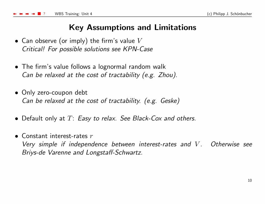
Key Assumptions and Limitations
• Can observe (or imply) the firm’s value VCritical! For possible solutions see KPN-Case
• The firm’s value follows a lognormal random walkCan be relaxed at the cost of tractability (e.g. Zhou).
• Only zero-coupon debtCan be relaxed at the cost of tractability. (e.g. Geske)
• Default only at T : Easy to relax. See Black-Cox and others.
• Constant interest-rates rVery simple if independence between interest-rates and V . Otherwise seeBriys-de Varenne and Longstaff-Schwartz.
10
➠ ➡➡ ➠ ■ ? WBS Training: Unit 4 (c) Philipp J. Schonbucher
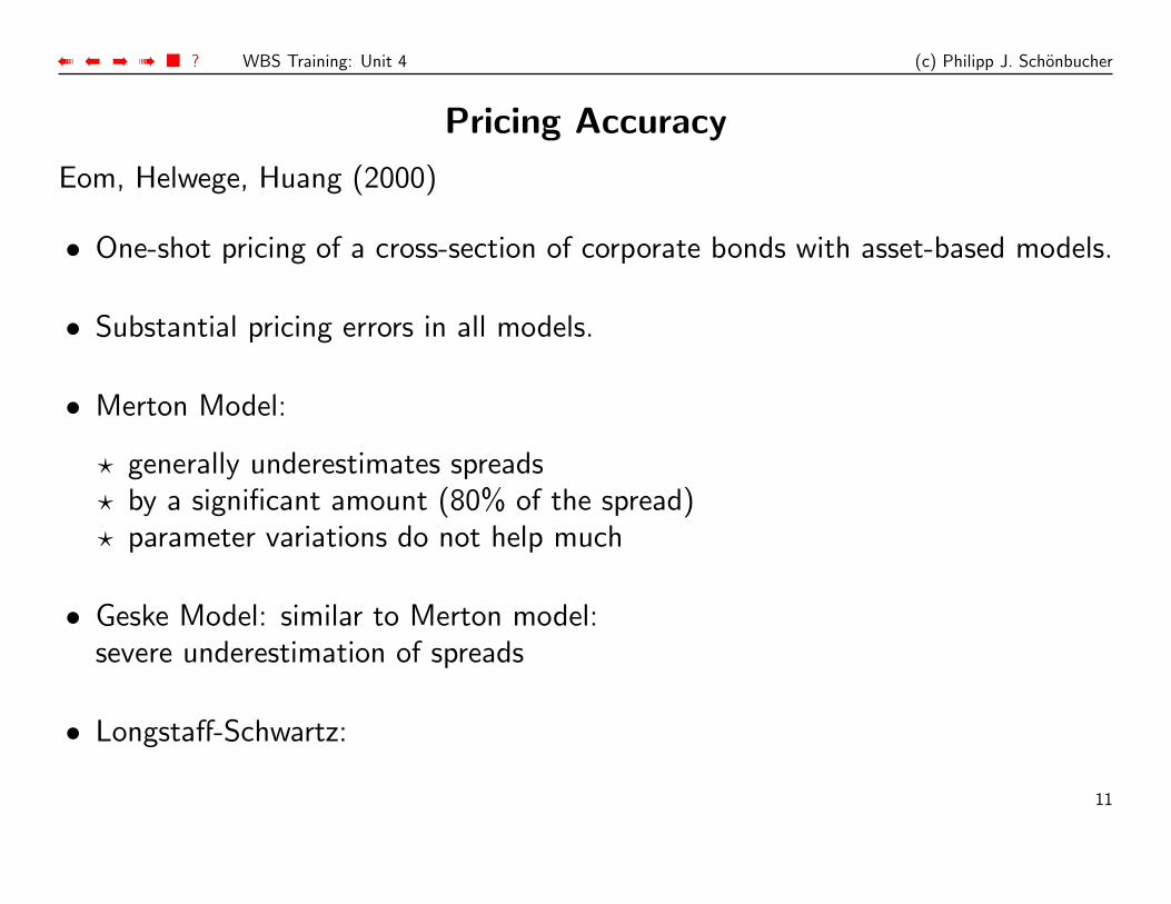
Pricing Accuracy
Eom, Helwege, Huang (2000)
• One-shot pricing of a cross-section of corporate bonds with asset-based models.
• Substantial pricing errors in all models.
• Merton Model:
? generally underestimates spreads? by a significant amount (80% of the spread)? parameter variations do not help much
• Geske Model: similar to Merton model:severe underestimation of spreads
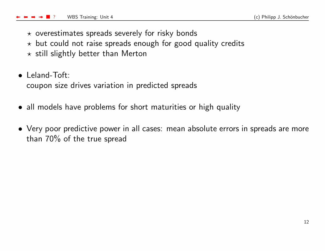
• Longstaff-Schwartz:
11
➠ ➡➡ ➠ ■ ? WBS Training: Unit 4 (c) Philipp J. Schonbucher
? overestimates spreads severely for risky bonds? but could not raise spreads enough for good quality credits? still slightly better than Merton
• Leland-Toft:coupon size drives variation in predicted spreads
• all models have problems for short maturities or high quality
• Very poor predictive power in all cases: mean absolute errors in spreads are morethan 70% of the true spread
12
➠ ➡➡ ➠ ■ ? WBS Training: Unit 4 (c) Philipp J. Schonbucher
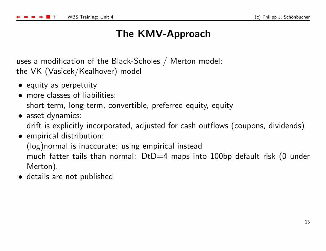
The KMV-Approach
uses a modification of the Black-Scholes / Merton model:the VK (Vasicek/Kealhover) model
• equity as perpetuity• more classes of liabilities:
short-term, long-term, convertible, preferred equity, equity• asset dynamics:
drift is explicitly incorporated, adjusted for cash outflows (coupons, dividends)• empirical distribution:
(log)normal is inaccurate: using empirical insteadmuch fatter tails than normal: DtD=4 maps into 100bp default risk (0 underMerton).
• details are not published
13
➠ ➡➡ ➠ ■ ? WBS Training: Unit 4 (c) Philipp J. Schonbucher
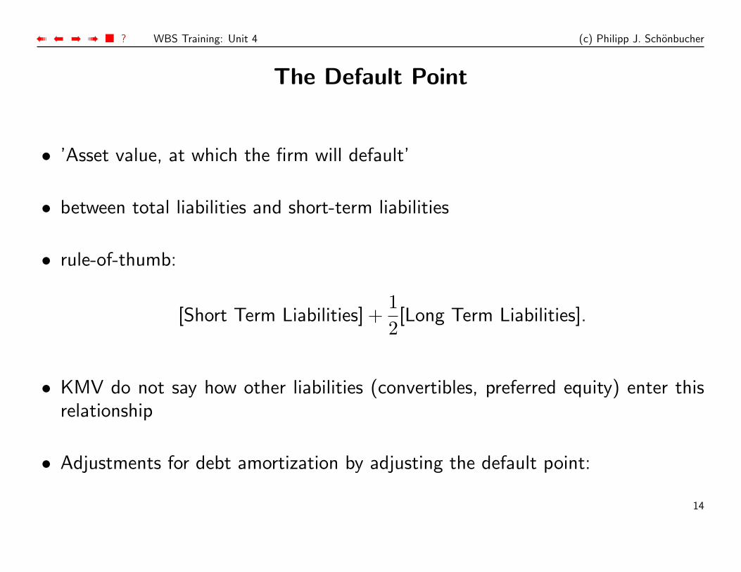
The Default Point
• ’Asset value, at which the firm will default’
• between total liabilities and short-term liabilities
• rule-of-thumb:
[Short Term Liabilities] +12[Long Term Liabilities].
• KMV do not say how other liabilities (convertibles, preferred equity) enter thisrelationship
• Adjustments for debt amortization by adjusting the default point:
14
➠ ➡➡ ➠ ■ ? WBS Training: Unit 4 (c) Philipp J. Schonbucher
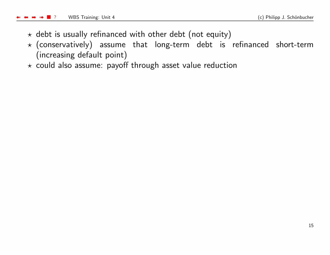
? debt is usually refinanced with other debt (not equity)? (conservatively) assume that long-term debt is refinanced short-term
(increasing default point)? could also assume: payoff through asset value reduction
15
➠ ➡➡ ➠ ■ ? WBS Training: Unit 4 (c) Philipp J. Schonbucher
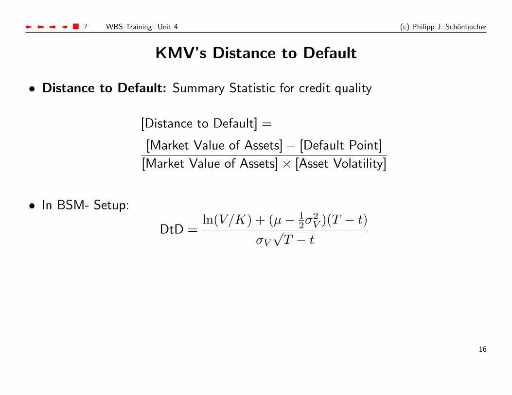
KMV’s Distance to Default
• Distance to Default: Summary Statistic for credit quality
[Distance to Default] =
[Market Value of Assets]− [Default Point]
[Market Value of Assets]× [Asset Volatility]
• In BSM- Setup:
DtD =ln(V/K) + (µ− 1
2σ2V )(T − t)
σV
√T − t
16
➠ ➡➡ ➠ ■ ? WBS Training: Unit 4 (c) Philipp J. Schonbucher
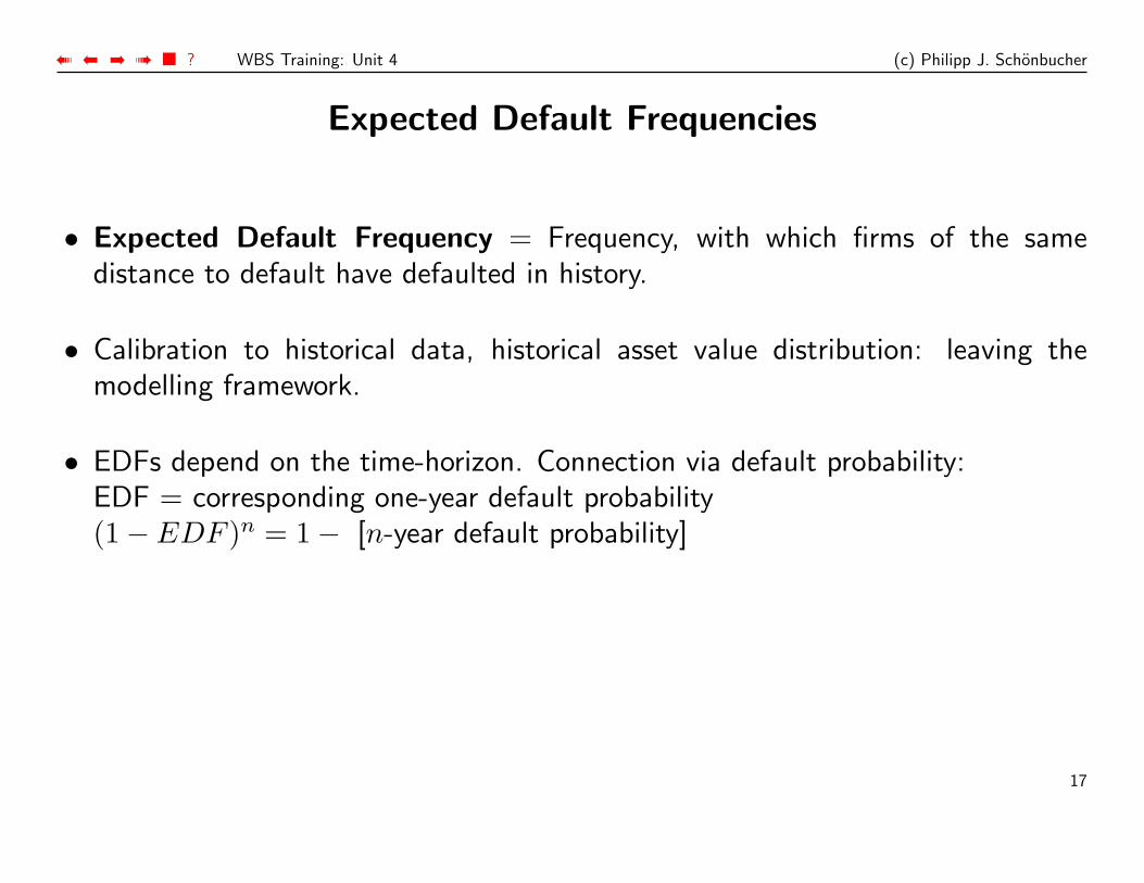
Expected Default Frequencies
• Expected Default Frequency = Frequency, with which firms of the samedistance to default have defaulted in history.
• Calibration to historical data, historical asset value distribution: leaving themodelling framework.
• EDFs depend on the time-horizon. Connection via default probability:EDF = corresponding one-year default probability(1− EDF )n = 1− [n-year default probability]
17
➠ ➡➡ ➠ ■ ? WBS Training: Unit 4 (c) Philipp J. Schonbucher
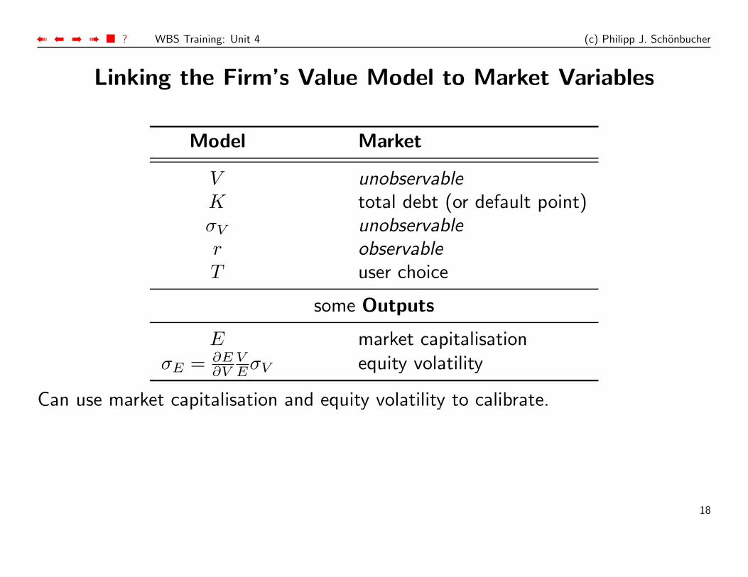
Linking the Firm’s Value Model to Market Variables
Model Market
V unobservableK total debt (or default point)σV unobservabler observableT user choice
some Outputs
E market capitalisationσE = ∂E
∂VVEσV equity volatility
Can use market capitalisation and equity volatility to calibrate.
18
➠ ➡➡ ➠ ■ ? WBS Training: Unit 4 (c) Philipp J. Schonbucher
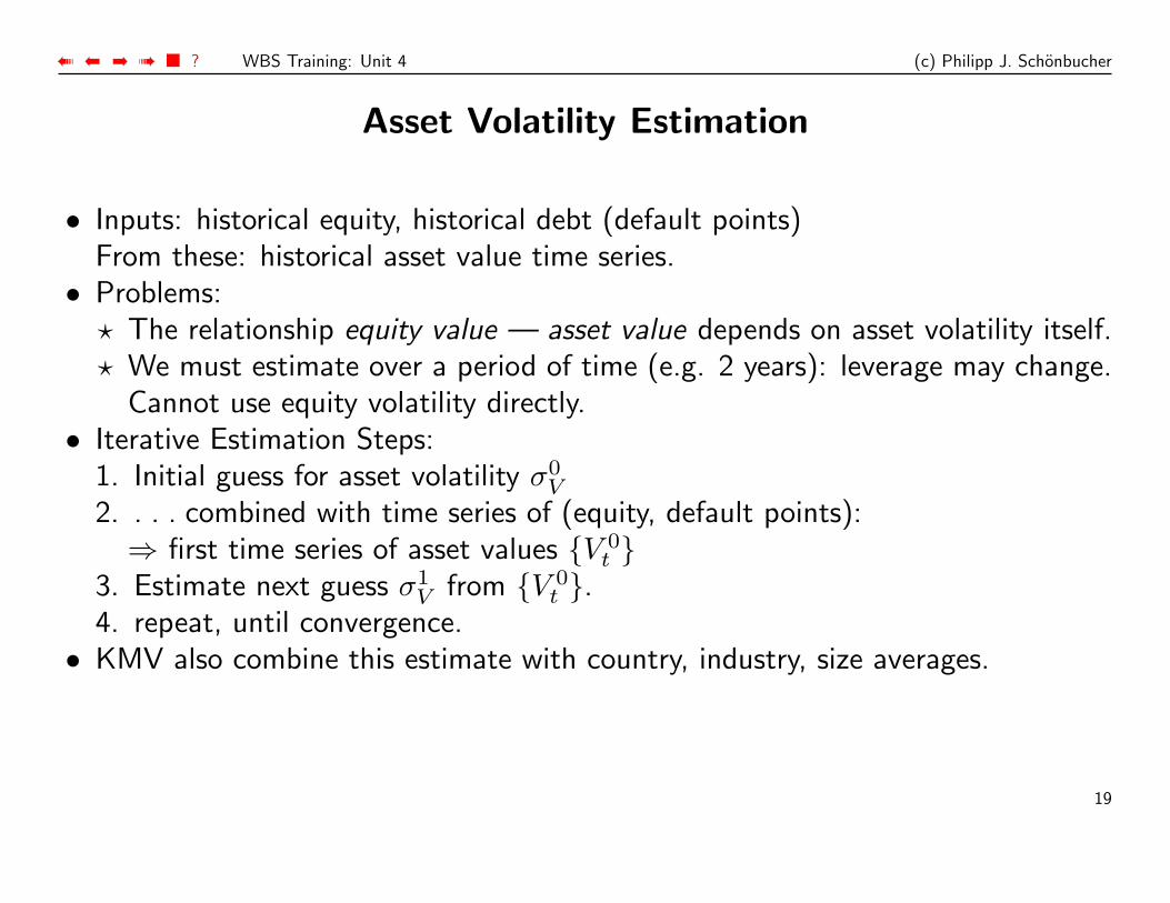
Asset Volatility Estimation
• Inputs: historical equity, historical debt (default points)From these: historical asset value time series.
• Problems:? The relationship equity value — asset value depends on asset volatility itself.? We must estimate over a period of time (e.g. 2 years): leverage may change.
Cannot use equity volatility directly.• Iterative Estimation Steps:
1. Initial guess for asset volatility σ0V
2. . . . combined with time series of (equity, default points):⇒ first time series of asset values {V 0
t }3. Estimate next guess σ1
V from {V 0t }.
4. repeat, until convergence.• KMV also combine this estimate with country, industry, size averages.
19
➠ ➡➡ ➠ ■ ? WBS Training: Unit 4 (c) Philipp J. Schonbucher
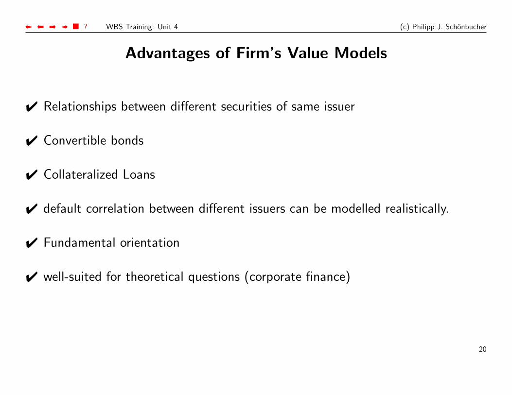
Advantages of Firm’s Value Models
✔ Relationships between different securities of same issuer
✔ Convertible bonds
✔ Collateralized Loans
✔ default correlation between different issuers can be modelled realistically.
✔ Fundamental orientation
✔ well-suited for theoretical questions (corporate finance)
20
➠ ➡➡ ➠ ■ ? WBS Training: Unit 4 (c) Philipp J. Schonbucher
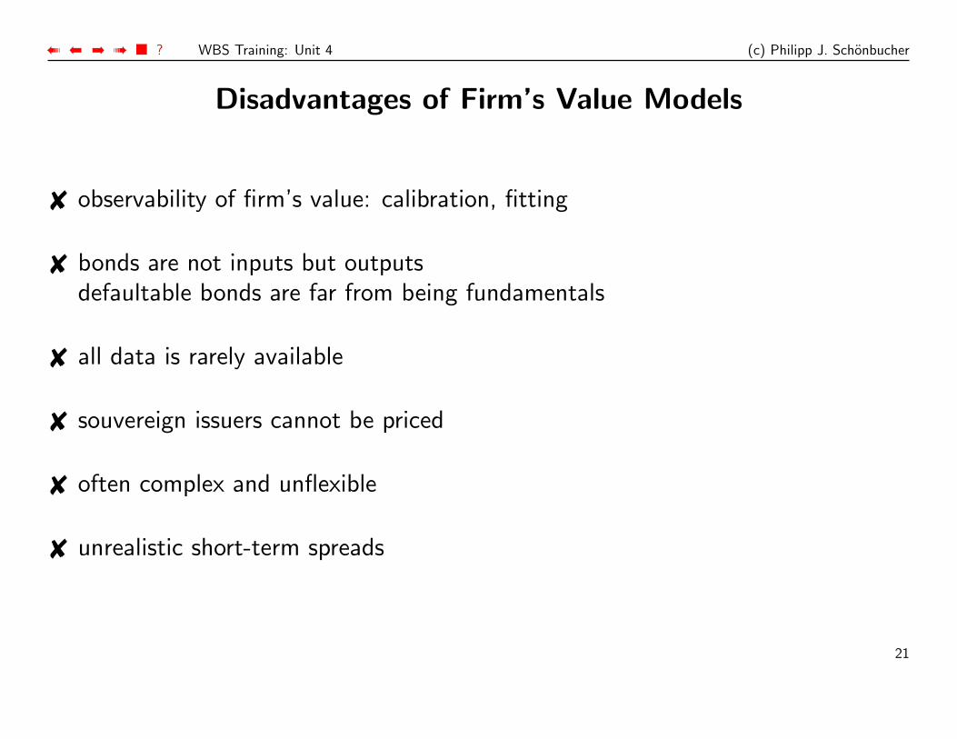
Disadvantages of Firm’s Value Models
✘ observability of firm’s value: calibration, fitting
✘ bonds are not inputs but outputsdefaultable bonds are far from being fundamentals
✘ all data is rarely available
✘ souvereign issuers cannot be priced
✘ often complex and unflexible
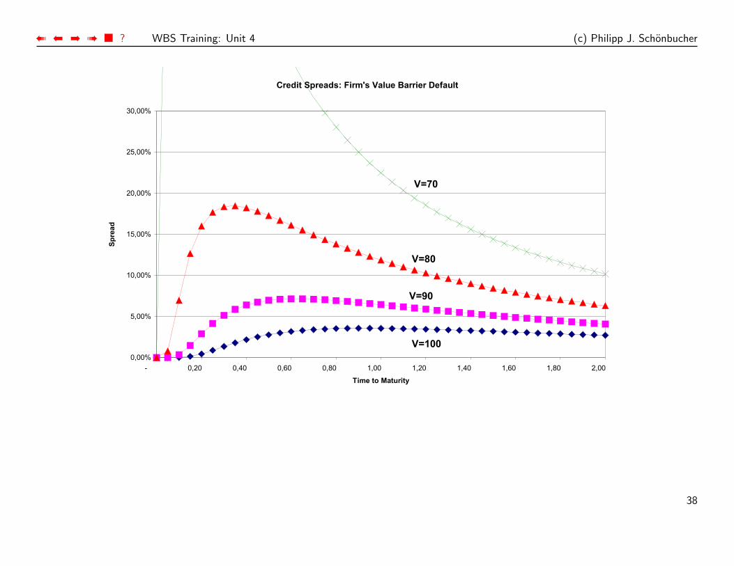
✘ unrealistic short-term spreads
21

➠ ➡➡ ➠ ■ ? WBS Training: Unit 4 (c) Philipp J. Schonbucher
Case Study: KPN
KPN is the former Dutch national telecommunications provider. The core businessareas are fixed network telephony (in the Netherlands), mobile communication anddata/IP services.
In the first half of 2000 KPN embarked upon an ambitious expansion course,mainly through the takeover of E-Plus (a German mobile phone provider) forwhich KPN paid EUR 9.1 bn in cash and EUR 9.9 bn in share conversion rights.The second large investment was the acqusition of a German UMTS license forwhich KPN paid EUR 6.5 bn (and its business partner 1.9 bn).
In this case study we try to analyse the effect of this on KPN’s credit risk using aMerton-type firm’s value model.
22
➠ ➡➡ ➠ ■ ? WBS Training: Unit 4 (c) Philipp J. Schonbucher
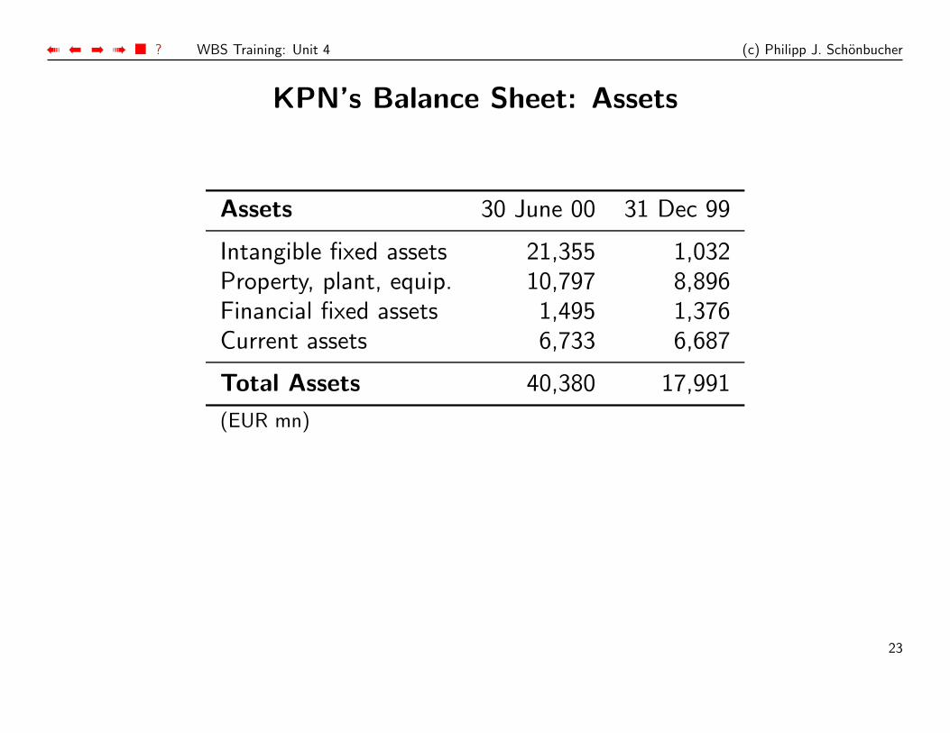
KPN’s Balance Sheet: Assets
Assets 30 June 00 31 Dec 99
Intangible fixed assets 21,355 1,032Property, plant, equip. 10,797 8,896Financial fixed assets 1,495 1,376Current assets 6,733 6,687
Total Assets 40,380 17,991
(EUR mn)
23
➠ ➡➡ ➠ ■ ? WBS Training: Unit 4 (c) Philipp J. Schonbucher
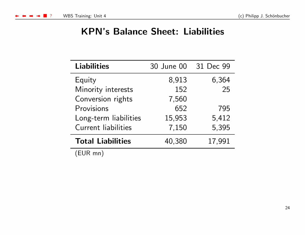
KPN’s Balance Sheet: Liabilities
Liabilities 30 June 00 31 Dec 99
Equity 8,913 6,364Minority interests 152 25Conversion rights 7,560Provisions 652 795Long-term liabilities 15,953 5,412Current liabilities 7,150 5,395
Total Liabilities 40,380 17,991
(EUR mn)
24
➠ ➡➡ ➠ ■ ? WBS Training: Unit 4 (c) Philipp J. Schonbucher
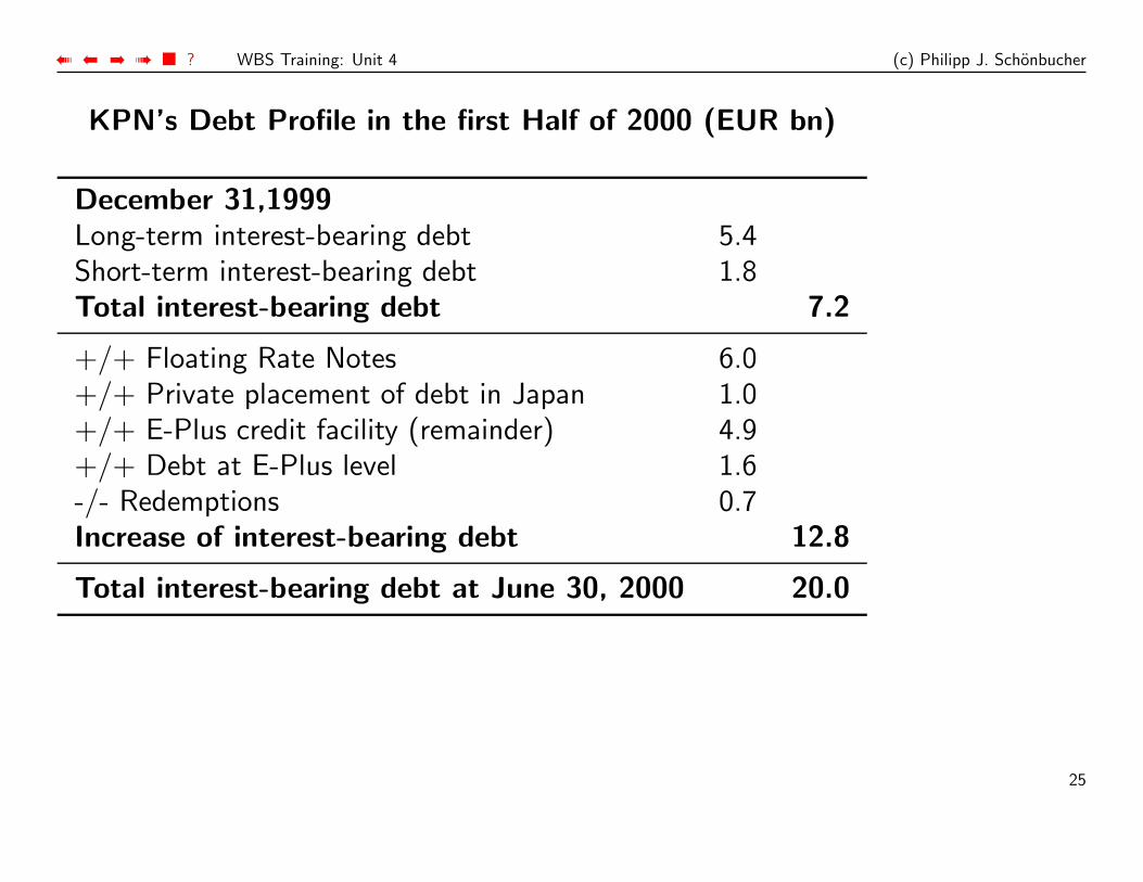
KPN’s Debt Profile in the first Half of 2000 (EUR bn)
December 31,1999Long-term interest-bearing debt 5.4Short-term interest-bearing debt 1.8Total interest-bearing debt 7.2
+/+ Floating Rate Notes 6.0+/+ Private placement of debt in Japan 1.0+/+ E-Plus credit facility (remainder) 4.9+/+ Debt at E-Plus level 1.6-/- Redemptions 0.7Increase of interest-bearing debt 12.8
Total interest-bearing debt at June 30, 2000 20.0
25
➠ ➡➡ ➠ ■ ? WBS Training: Unit 4 (c) Philipp J. Schonbucher
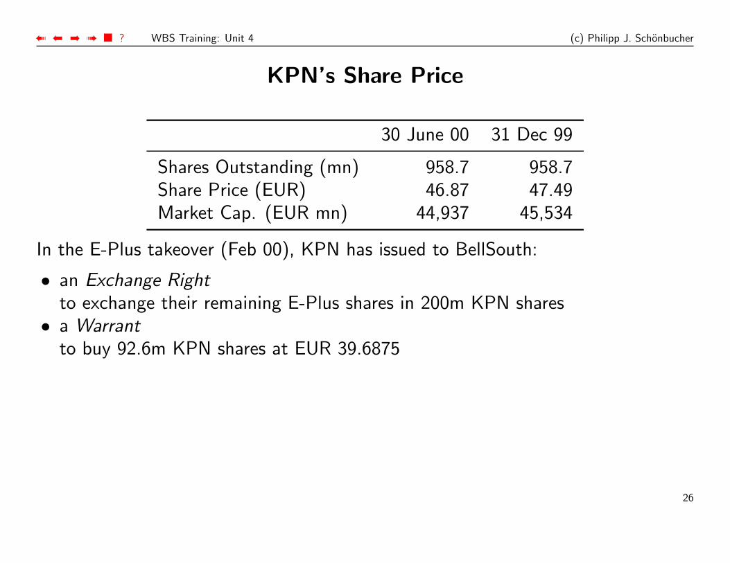
KPN’s Share Price
30 June 00 31 Dec 99
Shares Outstanding (mn) 958.7 958.7Share Price (EUR) 46.87 47.49Market Cap. (EUR mn) 44,937 45,534
In the E-Plus takeover (Feb 00), KPN has issued to BellSouth:
• an Exchange Rightto exchange their remaining E-Plus shares in 200m KPN shares
• a Warrantto buy 92.6m KPN shares at EUR 39.6875
26
➠ ➡➡ ➠ ■ ? WBS Training: Unit 4 (c) Philipp J. Schonbucher
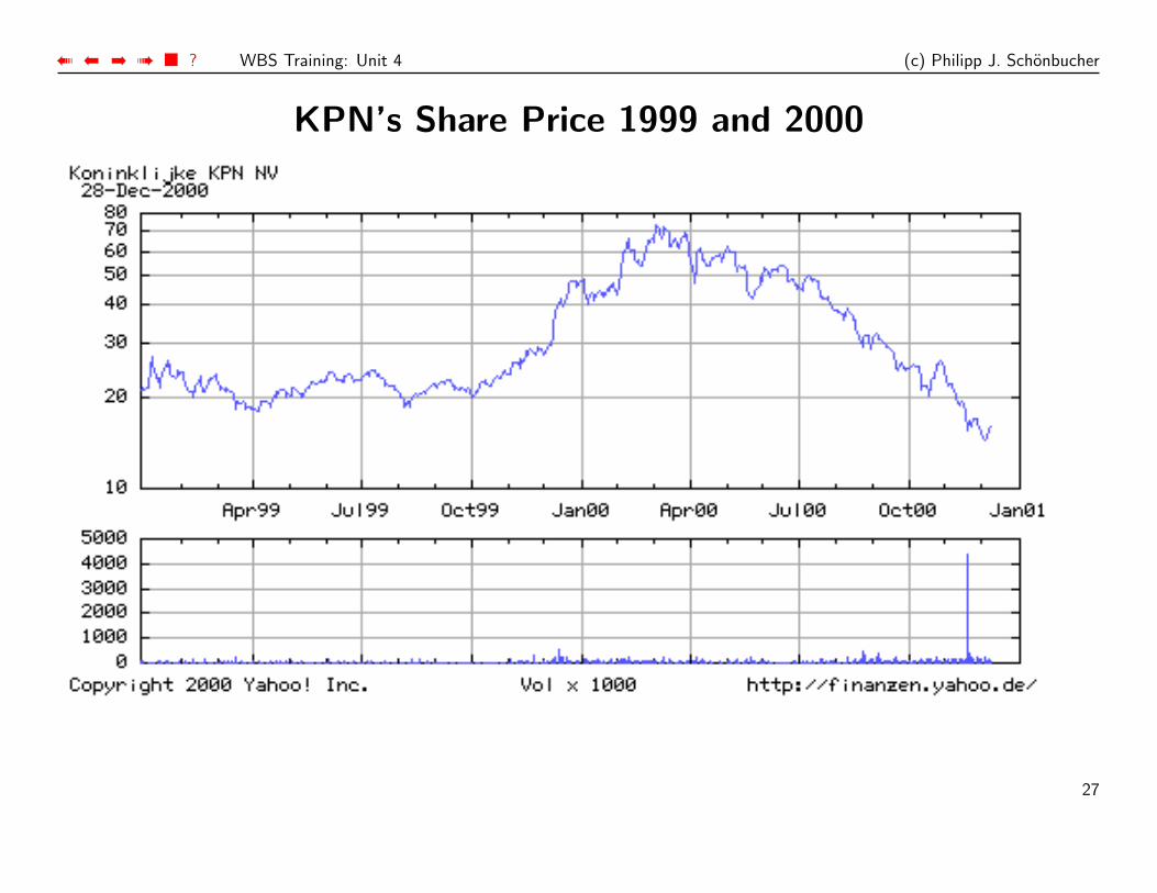
KPN’s Share Price 1999 and 2000
27
➠ ➡➡ ➠ ■ ? WBS Training: Unit 4 (c) Philipp J. Schonbucher
Case Study II: Enron
• 1986: Enron is formed.• 1989: international expansion begins• 1994: Enron starts electricity trading• 1996-1998: further international expansion. First off-balance-sheet partnerships
are formed.• 1999: Enron forms its broadband services unit, Enron online is formed• 2000: share price all-time high• Feb. 2001: Jeff Skilling CEO. EDF: 0.35%• Aug. 2001: Skiling resigns. EDF: 1.91%• Oct. 2001: the accounting scandal breaks. Investor confidence collapses.• Dec. 2nd, 2001: Enron files for Chapter 11.
28
➠ ➡➡ ➠ ■ ? WBS Training: Unit 4 (c) Philipp J. Schonbucher
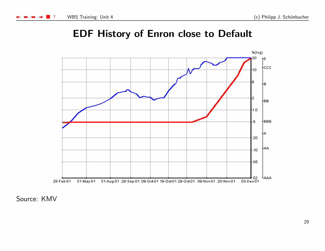
EDF History of Enron close to Default
Source: KMV
29
➠ ➡➡ ➠ ■ ? WBS Training: Unit 4 (c) Philipp J. Schonbucher
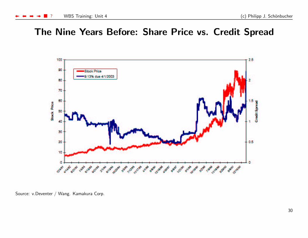
The Nine Years Before: Share Price vs. Credit Spread
Source: v.Deventer / Wang. Kamakura Corp.
30
➠ ➡➡ ➠ ■ ? WBS Training: Unit 4 (c) Philipp J. Schonbucher
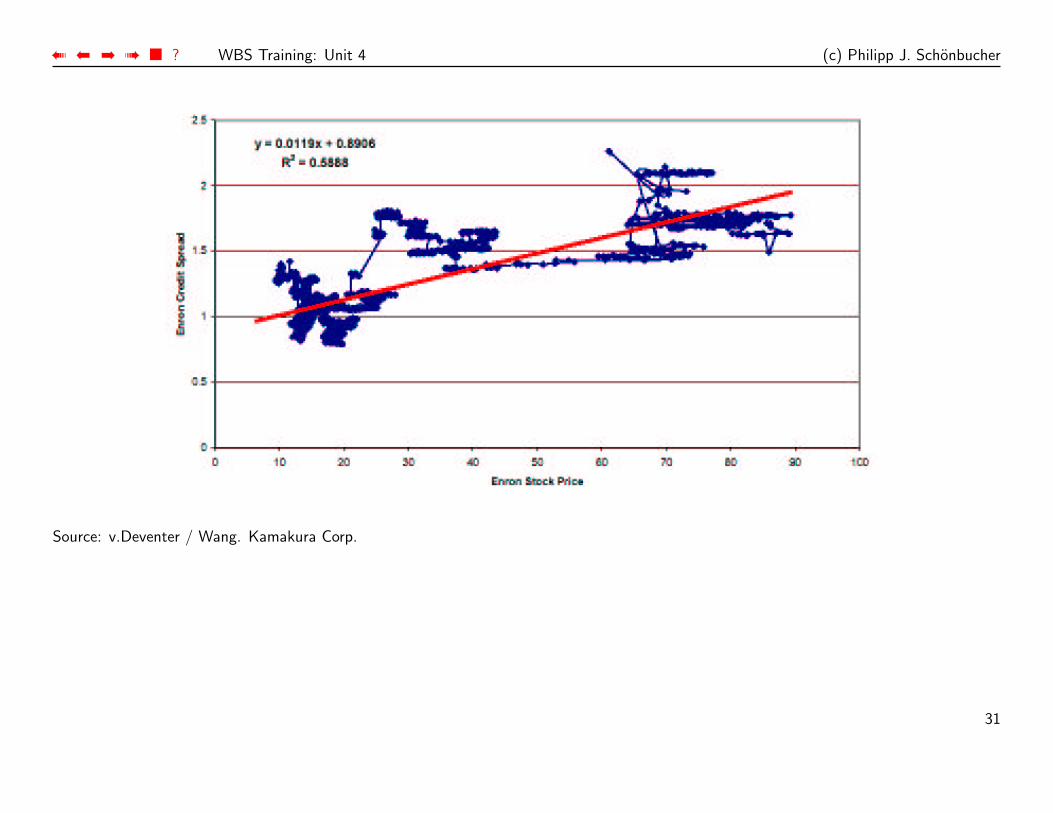
Source: v.Deventer / Wang. Kamakura Corp.
31
➠ ➡➡ ➠ ■ ? WBS Training: Unit 4 (c) Philipp J. Schonbucher
Statistical Investigation
the connection should be:
[Share] ⇑ [Spread] ⇓
This is true until end of 1997.
Regression results:
• For no bond did stock prices explain more than R2 < 59% of the spreads.• Slightly better results for changes in share prices and spreads: 4 out of 8
bonds had consistent directions with share price movements. (2 of them withsignificant coefficients)
• Out of 16.200 data points (spread observations), 46% were consistent with theMerton model.
• generally very poor explainatory power
32
➠ ➡➡ ➠ ■ ? WBS Training: Unit 4 (c) Philipp J. Schonbucher
Discussion: What went Wrong?
• Accountancy fraud does not even factor here (yet).• Problem: DotCom-Bubble:
? irrationally inflated share prices? no more indicators of value of the firm’s assets? only indicate expectation to “find a bigger fool”
• Better results outside of bubble. But how do we recognize a bubble in advance?!• Hedging performance (1st differences) not good.
33
➠ ➡➡ ➠ ■ ? WBS Training: Unit 4 (c) Philipp J. Schonbucher
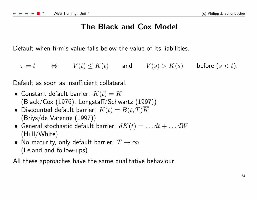
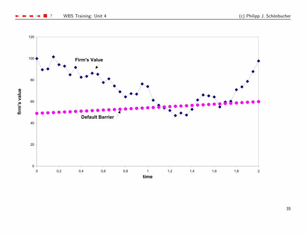
The Black and Cox Model
Default when firm’s value falls below the value of its liabilities.
τ = t ⇔ V (t) ≤ K(t) and V (s) > K(s) before (s < t).
Default as soon as insufficient collateral.
• Constant default barrier: K(t) = K(Black/Cox (1976), Longstaff/Schwartz (1997))
• Discounted default barrier: K(t) = B(t, T )K(Briys/de Varenne (1997))
• General stochastic default barrier: dK(t) = . . . dt + . . . dW(Hull/White)
• No maturity, only default barrier: T →∞(Leland and follow-ups)
All these approaches have the same qualitative behaviour.
34
➠ ➡➡ ➠ ■ ? WBS Training: Unit 4 (c) Philipp J. Schonbucher
35
➠ ➡➡ ➠ ■ ? WBS Training: Unit 4 (c) Philipp J. Schonbucher
Default Costs
If V (and K) has continuous paths, we are able to predict the default-value of Vone moment before default.
Need default costs to have loss in default or stochastic (or lower) recoveries.
Payoff of bonds:
K at maturity T , if there was no default previously: τ > T
cB(τ, T ) at τ , if default before maturity: τ ≤ T .
c as in recovery models for intensity.
36
➠ ➡➡ ➠ ■ ? WBS Training: Unit 4 (c) Philipp J. Schonbucher
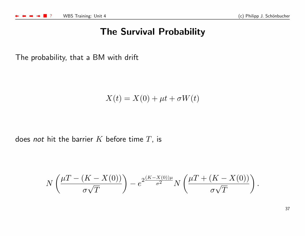
The Survival Probability
The probability, that a BM with drift
X(t) = X(0) + µt + σW (t)
does not hit the barrier K before time T , is
N
(µT − (K −X(0))
σ√
T
)− e
2(K−X(0))µ
σ2 N
(µT + (K −X(0))
σ√
T
).
37
➠ ➡➡ ➠ ■ ? WBS Training: Unit 4 (c) Philipp J. Schonbucher
38
➠ ➡➡ ➠ ■ ? WBS Training: Unit 4 (c) Philipp J. Schonbucher
How to avoid zero short-term spreads?
Cause: If there is a finite distance to the barrier, a continuous process cannotreach it in the next instance.
• Introduce jumps in the firm’s value V(Zhou 2001)
• Maybe the default barrier is indeed closer than we thought.Duffie/Lando (1997), and partially: Giesecke (2002), Finkelstein, Lardy et.al.(2002)
39
➠ ➡➡ ➠ ■ ? WBS Training: Unit 4 (c) Philipp J. Schonbucher
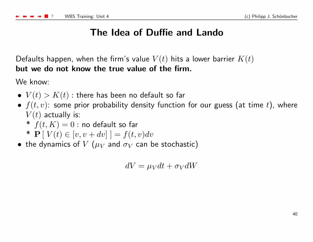
The Idea of Duffie and Lando
Defaults happen, when the firm’s value V (t) hits a lower barrier K(t)but we do not know the true value of the firm.
We know:
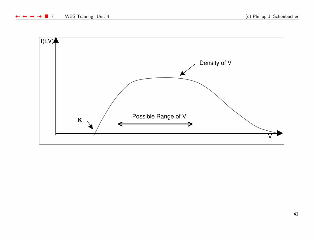
• V (t) > K(t) : there has been no default so far• f(t, v): some prior probability density function for our guess (at time t), where
V (t) actually is:* f(t, K) = 0 : no default so far* P [ V (t) ∈ [v, v + dv] ] = f(t, v)dv
• the dynamics of V (µV and σV can be stochastic)
dV = µV dt + σV dW
40
➠ ➡➡ ➠ ■ ? WBS Training: Unit 4 (c) Philipp J. Schonbucher
Density of V
V
f(t,V)
KPossible Range of V
41
➠ ➡➡ ➠ ■ ? WBS Training: Unit 4 (c) Philipp J. Schonbucher
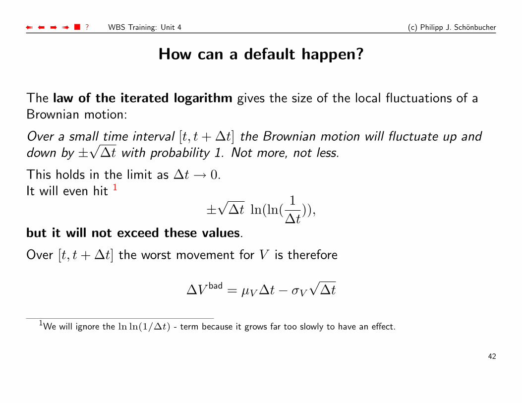
How can a default happen?
The law of the iterated logarithm gives the size of the local fluctuations of aBrownian motion:
Over a small time interval [t, t + ∆t] the Brownian motion will fluctuate up anddown by ±
√∆t with probability 1. Not more, not less.
This holds in the limit as ∆t → 0.It will even hit 1
±√
∆t ln(ln(1
∆t)),
but it will not exceed these values.
Over [t, t + ∆t] the worst movement for V is therefore
∆V bad = µV ∆t− σV
√∆t
1We will ignore the ln ln(1/∆t) - term because it grows far too slowly to have an effect.
42

➠ ➡➡ ➠ ■ ? WBS Training: Unit 4 (c) Philipp J. Schonbucher
If we can observe V with certainty, there are two cases:
(i) V (t) > K + σV
√∆t:
V is too far away from the barrier. No default will happen, even for theworst-case movement.
(ii) K < V (t) ≤ K + σV
√∆t:
V is very close to the barrier. Here a default can happen over the next timestep. As ∆t → 0 we know, that it will indeed happen.
43
➠ ➡➡ ➠ ■ ? WBS Training: Unit 4 (c) Philipp J. Schonbucher
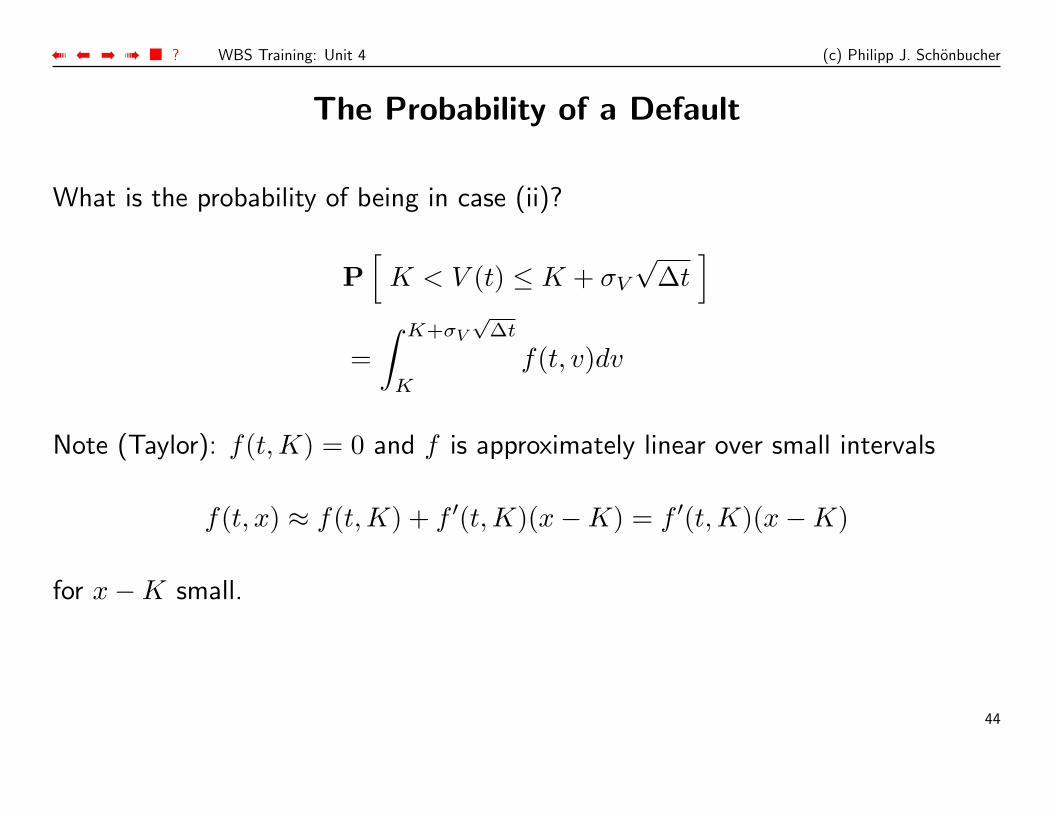
The Probability of a Default
What is the probability of being in case (ii)?
P[
K < V (t) ≤ K + σV
√∆t
]=
∫ K+σV
√∆t
K
f(t, v)dv
Note (Taylor): f(t, K) = 0 and f is approximately linear over small intervals
f(t, x) ≈ f(t, K) + f ′(t, K)(x−K) = f ′(t, K)(x−K)
for x−K small.
44
➠ ➡➡ ➠ ■ ? WBS Training: Unit 4 (c) Philipp J. Schonbucher
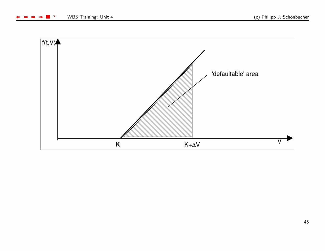
V
f(t,V)
K K+∆V
'defaultable' area
45
➠ ➡➡ ➠ ■ ? WBS Training: Unit 4 (c) Philipp J. Schonbucher
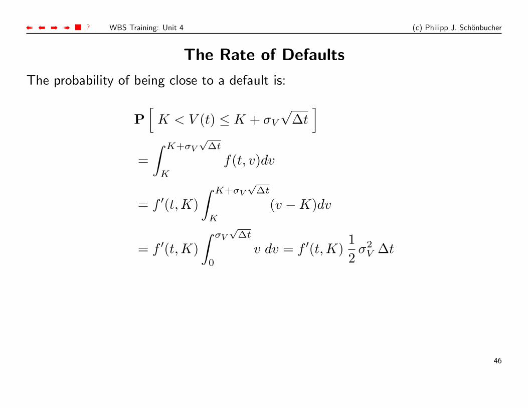
The Rate of Defaults
The probability of being close to a default is:
P[
K < V (t) ≤ K + σV
√∆t
]=
∫ K+σV
√∆t
K
f(t, v)dv
= f ′(t, K)∫ K+σV
√∆t
K
(v −K)dv
= f ′(t, K)∫ σV
√∆t
0
v dv = f ′(t, K)12
σ2V ∆t
46
➠ ➡➡ ➠ ■ ? WBS Training: Unit 4 (c) Philipp J. Schonbucher
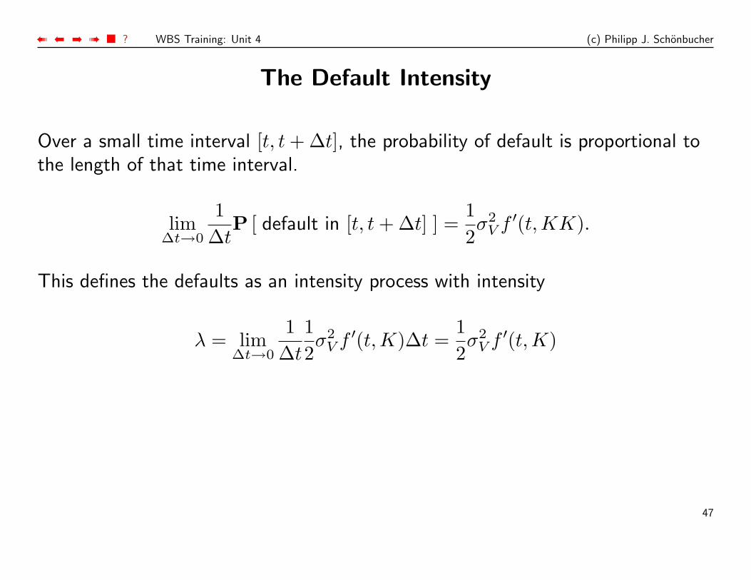
The Default Intensity
Over a small time interval [t, t + ∆t], the probability of default is proportional tothe length of that time interval.
lim∆t→0
1∆t
P [ default in [t, t + ∆t] ] =12σ2
V f ′(t, KK).
This defines the defaults as an intensity process with intensity
λ = lim∆t→0
1∆t
12σ2
V f ′(t, K)∆t =12σ2
V f ′(t, K)
47
➠ ➡➡ ➠ ■ ? WBS Training: Unit 4 (c) Philipp J. Schonbucher
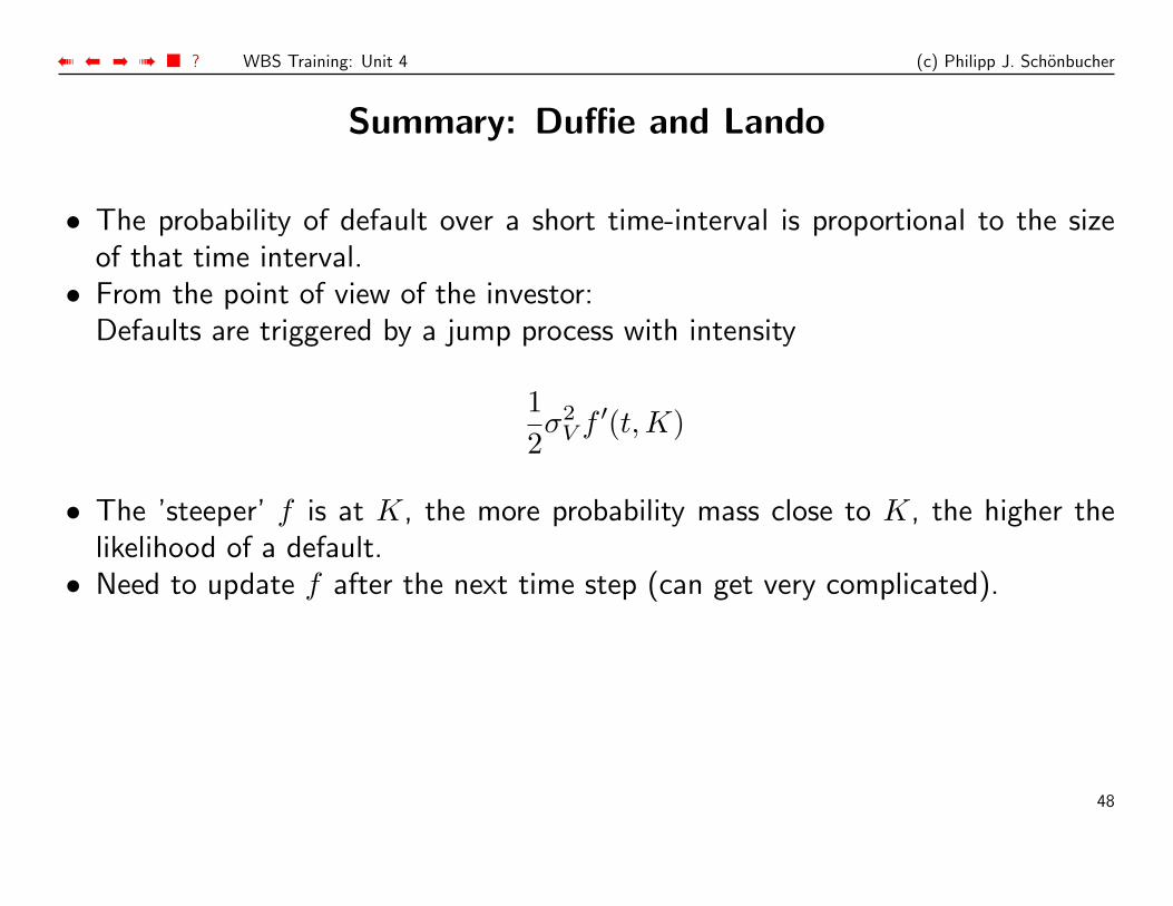
Summary: Duffie and Lando
• The probability of default over a short time-interval is proportional to the sizeof that time interval.
• From the point of view of the investor:Defaults are triggered by a jump process with intensity
12σ2
V f ′(t, K)
• The ’steeper’ f is at K, the more probability mass close to K, the higher thelikelihood of a default.
• Need to update f after the next time step (can get very complicated).
48
➠ ➡➡ ➠ ■ ? WBS Training: Unit 4 (c) Philipp J. Schonbucher
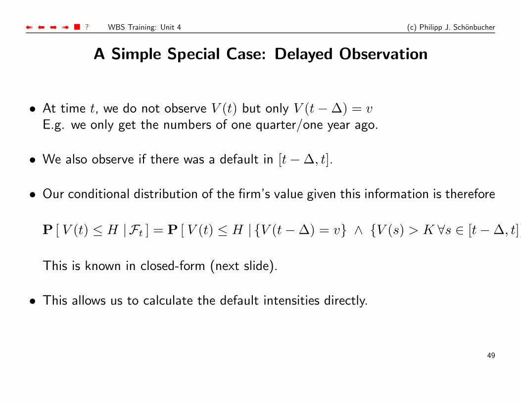
A Simple Special Case: Delayed Observation
• At time t, we do not observe V (t) but only V (t−∆) = vE.g. we only get the numbers of one quarter/one year ago.
• We also observe if there was a default in [t−∆, t].
• Our conditional distribution of the firm’s value given this information is therefore
P [ V (t) ≤ H | Ft ] = P [ V (t) ≤ H | {V (t−∆) = v} ∧ {V (s) > K ∀s ∈ [t−∆, t]} ]
This is known in closed-form (next slide).
• This allows us to calculate the default intensities directly.
49

➠ ➡➡ ➠ ■ ? WBS Training: Unit 4 (c) Philipp J. Schonbucher
The Joint Distribution
Let dV/V = µdt + σdW , V (0) = V0 and mV (T ) := mint≤T V (t). Then
P [ V (T ) ≥ H ∧ mV (T ) ≥ K ] = N(d3)−(
K
V0
)(2µ/σ2)−1
N(d4)
where
d3 =ln(V0/H) + (µ− 1
2σ2)T
σ√
T
d4 =ln(K2/(V0H)) + (µ− 1
2σ2)T
σ√
T.
50
➠ ➡➡ ➠ ■ ? WBS Training: Unit 4 (c) Philipp J. Schonbucher
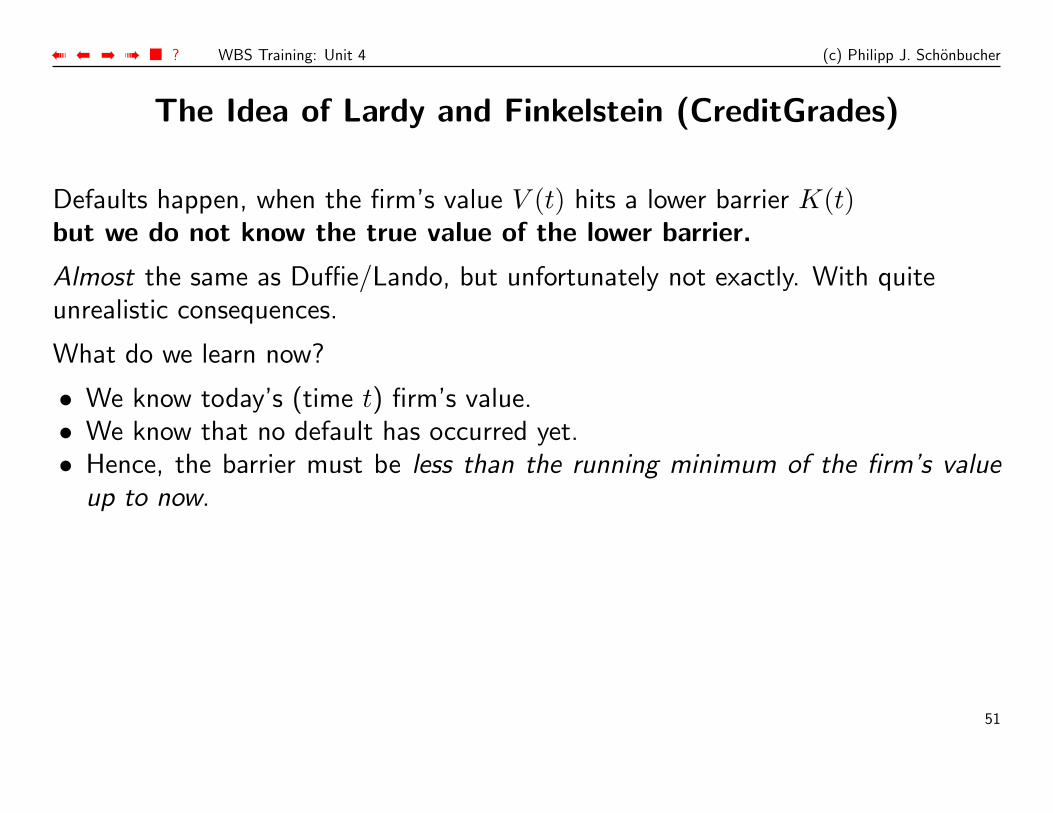
The Idea of Lardy and Finkelstein (CreditGrades)
Defaults happen, when the firm’s value V (t) hits a lower barrier K(t)but we do not know the true value of the lower barrier.
Almost the same as Duffie/Lando, but unfortunately not exactly. With quiteunrealistic consequences.
What do we learn now?
• We know today’s (time t) firm’s value.• We know that no default has occurred yet.• Hence, the barrier must be less than the running minimum of the firm’s value
up to now.
51
➠ ➡➡ ➠ ■ ? WBS Training: Unit 4 (c) Philipp J. Schonbucher
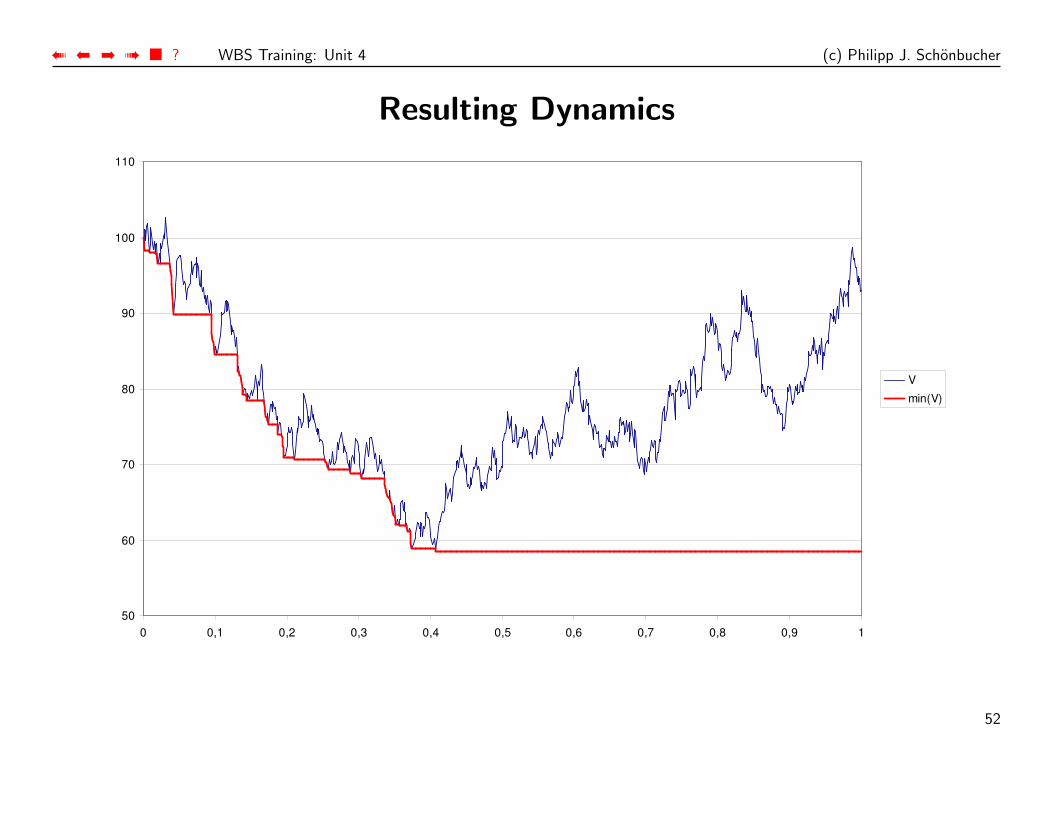
Resulting Dynamics
50
60
70
80
90
100
110
0 0,1 0,2 0,3 0,4 0,5 0,6 0,7 0,8 0,9 1
V
min(V)
52
➠ ➡➡ ➠ ■ ? WBS Training: Unit 4 (c) Philipp J. Schonbucher
Results: Dynamics
(see Giesecke (2002))
• The default compensator behaves like the running maximum of a diffusionprocess.
• The time of default is totally inaccessible, but
• a default intensity does not exist.
• Unless V equals its current running minimum, we again have zero short-termcredit spreads.
• At t = 0, there is a discrete, positive probability of default.
53
➠ ➡➡ ➠ ■ ? WBS Training: Unit 4 (c) Philipp J. Schonbucher
• The model should not be used for hedging: The spreads change shape drastically(and unrealistically) at t = 0.
• For credit pricing at t = 0 the model may just be acceptable (because it isreduced to Duffie/Lando with delayed observation).
• A US patent application has been filed for CreditGrades.Personally, I disapprove of this.
• My advice:Duffie/Lando with delayed observations is better anyway.
54
➠ ➡➡ ➠ ■ ? WBS Training: Unit 4 (c) Philipp J. Schonbucher
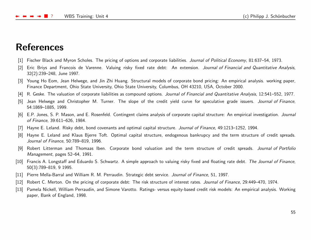
References[1] Fischer Black and Myron Scholes. The pricing of options and corporate liabilities. Journal of Political Economy, 81:637–54, 1973.
[2] Eric Briys and Francois de Varenne. Valuing risky fixed rate debt: An extension. Journal of Financial and Quantitative Analysis,32(2):239–248, June 1997.
[3] Young Ho Eom, Jean Helwege, and Jin Zhi Huang. Structural models of corporate bond pricing: An empirical analysis. working paper,Finance Department, Ohio State University, Ohio State University, Columbus, OH 43210, USA, October 2000.
[4] R. Geske. The valuation of corporate liabilities as compound options. Journal of Financial and Quantitative Analysis, 12:541–552, 1977.
[5] Jean Helwege and Christopher M. Turner. The slope of the credit yield curve for speculative grade issuers. Journal of Finance,54:1869–1885, 1999.
[6] E.P. Jones, S. P. Mason, and E. Rosenfeld. Contingent claims analysis of corporate capital structure: An empirical investigation. Journalof Finance, 39:611–626, 1984.
[7] Hayne E. Leland. Risky debt, bond covenants and optimal capital structure. Journal of Finance, 49:1213–1252, 1994.
[8] Hayne E. Leland and Klaus Bjerre Toft. Optimal capital structure, endogenous bankrupcy and the term structure of credit spreads.Journal of Finance, 50:789–819, 1996.
[9] Robert Litterman and Thomaas Iben. Corporate bond valuation and the term structure of credit spreads. Journal of PortfolioManagement, pages 52–64, 1991.
[10] Francis A. Longstaff and Eduardo S. Schwartz. A simple approach to valuing risky fixed and floating rate debt. The Journal of Finance,50(3):789–819, 9 1995.
[11] Pierre Mella-Barral and William R. M. Perraudin. Strategic debt service. Journal of Finance, 51, 1997.
[12] Robert C. Merton. On the pricing of corporate debt: The risk structure of interest rates. Journal of Finance, 29:449–470, 1974.
[13] Pamela Nickell, William Perraudin, and Simone Varotto. Ratings- versus equity-based credit risk models: An empirical analysis. Workingpaper, Bank of England, 1998.
55
➠ ➡➡ ➠ ■ ? WBS Training: Unit 4 (c) Philipp J. Schonbucher
[14] L.T. Nielsen, J. Saa-Requejo, and P. Santa-Clara. Default risk and interest rate risk: The term structure of default spreads. Workingpaper, INSEAD, 1993.
[15] Joseph P. Ogden. Determinants of the ratings and yields of corporate bonds: Tests of the contingent claims model. The Journal ofFinancial Research, 10:329–339, 1987.
[16] Oded Sarig and Arthur Warga. Some empirical estimates of the risk structure of interest rates. Journal of Finance, 44:1351–1360, 1989.
[17] David Guoming Wei and Dajiang Guo. Pricing risky debt: An empirical comparison of the Longstaff and Schwartz and Merton models.Journal of Fixed Income, 7:8–28, 1997.
[18] Chunsheng Zhou. A jump-diffusion approach to modeling credit risk and valuing defaultable securities. Finance and EconomicsDiscussion Paper Series 1997/15, Board of Governors of the Federal Reserve System, March 1997.
56