The maximum of a number of independent residual waiting times

by PAUL VAN BEEK*

1. Introduction

Consider n stationary alternating renewal-processes which are mutually independent. In each process periods of the first type alternate with periods of the second type.

Assume that we start observing the process at time zero. Let y , denote the waiting time until a period of the first type appears in the ith process for the first time and Put

- w = max (y,). 1 6 i S n

The corresponding distribution functions and densities are denoted W,, w, and W, w, respectively. We derive formulae which furnish approximations for the mean and variance of w , knowing only the means and variances of the y,.

The method we use in the sequel will now be explained briefly. Rather than present assertions valid for a particular class of distribution functions, we have found it easier to choose and work with a representative of this class. In the case under consideration. the final result does not depend too much on the specific choice of this distribution function. For that reason, we can speak here of some kind of “invariance”.

This method has been applied succesfully by the author in other cases. As an interesting application we mention the manufacture of a product consisting

of a number of components which have a positive probability of being out of stock. With the means developed in the sequel, we will be able to calculate approximately the mean and variance of the time you have to wait for the next possible manufactur- ing of the product.

These results will be used in the control part of a Management Information System (IPSO) developed within the N.V. Philips’ Gloeilampenfabrieken in Eindhoven.

2. Derivation of the stationary waiting time distributions

Let the lengths of the first and second type periods of the ith process be l it and li2, having continuous distribution functions F, , and Fi2, means pi, and pi2 and variances oft and of,, respectively. For the sake of simplicity we shall assume that the third moment of F,, exists.

The distribution function U of the forward recurrence time g of a stationary renewal process with distribution function G having mean p, follows from

Philip ISA-R, VN-6, Eindhovcn, The Netherlands.

STATISTICA NEERLANDICA 27 (1973) NR. 2 59

In the present situation we are confronted with alternating renewal processes. There- fore we must also consider the times we need not wait at all:

We then have:

1 " PilfPi2 Pil+Pi2 0 s [I -&2(Y)l dY. w,(x) = ~ + ~

Pi 1

Here we have used the fact that:

Pi2 P(w, = 0) = ___ "l and P(_wi #O) =-. Pi1 +Pi2 Pit +Pi2

From the independence of the processes we have:

Let the means and variances of _w. w,, ..., _w,, be p, pl, ..., pn and a', a:, ..., a,, 2

respectively. The pi and a: can be expressed as functions of pil, pi2, ai2 and Ti2,

where 00

T~~ = x3dFr2(x),i = 1 ,..., n. 0

The following expressions can easily be obtained, remembering that

STATISTICA NEERLANDICA 27 (1973) NR. 2

3. An approximation of p and a*

First of all we give an example which shows that direct calculation of p and o2 using (3) is cumbersome because of combinatorial difficulties.

Let 1 1

pil = - and F,,(x) = 1 -e-B'x with pi, = - I

a, Pi Here we have

Mi e - B i x W ( x ) = n 1 -- i = " I ( %+Pi

and after evaluation we obtain 2" different terms. It is this fact that creates difficulties. We define a class C of densitiesf which can be written in the following form:

f ( x ) = aSo(x) + ( I - a)g(x) with 0 5 u s 1,

So the 'density' with the probability concentrated at x = 0 and g, such that

(i) g(x) = 0, x < 0, m m

(ii) g(x)dx = 1 and x2g(x)dx < a, 0 0

(iii) 0 5 x s y => g(x) r g(y),

(iv) limg(x) = g(o). XI0

The densities wi belong to C. The idea is now the following: Select a very simple density in C, e.g.:

1-a f , b ( X ) = + b, O s x < b

0 elsewhere.

The corresponding distribution function is

- -

The mean and variance pL,,b and t& respectively are

STATLWICA NEERLANDICA 27 (1973) NR. 2 61

The following relations can easily be obtained :

Before continuing we will prove the following lemma:

Lemma

Let ftz C and

m m p = xf(x)dx, s2 = x2f(x)dx and a2 = s 2 2 - p .

0 0

Then we have the following inequality:

p 2 S; 3a2 or equivalently 4p2 5 3s’. (8)

There is equality in (8) if and only iff is of the form (4) with a = 0 and arbitrary b > 0.

Proof

Let f ( x ) = aSo(x) + (1 - a)g(x). We can restrict ourselves to densities frz C with a = 0 as:

m m

x2g(x) dx x2g(x) dx

[ i xg(x)dx]2 - [ 1 xg(x) dx]” r 0 O 5 a < l . -- 1 0 -- S2

”

Thus we may assume f ( x ) = g(x). We now have :

m m

/A = xf(x)dx = - + J x2df(x) 0 0

and 4) m

s2 = J x’f(x) dx = -3 J x3 df(x). 0 0

STATISTEA NEERLANDICA 27 (1973) NR. 2 62

Because f is monotonely decreasing we can define the following finite measure G on [0, 00) :

G(A) = - jdf(x), where A is a measurable set. A

Thus m m

p = 3 x2 dG(x) and s2 = 3 j x3 dG(x). 0 0

From Schwarz’ Inequality we obtain

2 0 0 m

5 j x dG(x)- j x3 dG(x). 0 0

so 4p2 5 3s2.

Now assume equality in (8). Then we have

([ x2 dG(x)) = S, x dG(x)* J x3 dG(x). 0

And this equality implies that there exists a constant b e R+ such that

x * = bx* or x = b for all x > 0,

except on a set A such that G(A) = 0. But this implies that G is concentrated a t x = b .

Further

and this implies that f is the rectangular density on [0, b]. Q.E.D.

that By the lemma it is possible to select numbers a,, with 0 5 a, 5 1 and b, 2 0 such

3 4 - p; 30; + 3p; 2PLi

30; + 3p; a, = and b, = (9)

We now introduce random variables _wp having distribution functions Fol,b,.

Fal,bl(x) F,,,,~,(x) is the distribution function of max (_wp, ~ 9 ) ) : Now with b, S bj the following formulae are easily derived (using the remark that

STAATISTICA NEERLANDICA 27 (1973) NR 2 63

bi -(a,bi( 1 - a j ) + a jb j ( 1 - ai)) + 2bj

2b: (1 - a j ) (b; - b:) -(l-U,)(l-aj) + 3bj 2bj

and E(max2(_wo, w?)) =

b2 3bj f (a,b,( 1 - aj) + ajbj(1- aj)) + b3 2bj 3bj

(1 - aj ) ( b j - b,J) -+l-aj)(l-aj) +

We now are able to set up the following calculation scheme for computing the first two moments of max (yl, . . ., _wn). We make use of the following identity:

max(y,, ..., wk) = max(max(qy,, ..., E ~ - ~ ) , wk), 2 5 k n.

We proceed as follows:

1. Suppose that we already know an approximation for the mean p and variance a2 of max (yl, . . ., 4yk- l). Now we calculate numbers a and b such that

3a2 - p 2

3a2 + 3p2 2P

3a2 + 3p2 a = -___ and b =

2. Calculate numbers ak and b, from (9). 3. Calculate the first two moments of the distribution function Fa,b(x)Fak,bk(x)

according to (10) and (1 1) by replacing a,, bi, aj, bj by a, b, a, and b, respectively. 4. Use these moments as approximations to the corresponding moments of

max (wl , . . .) &k)* Starting with k = 2 we get ultimately approximations of the first two moments of max (wl , . . ., Yn)*

This calculation scheme gives us no guarantee that the quantity a is positive. It is a curious fact that although a < O has no significance in probabilistic sense, we can obtain reasorrsbly good results by applying (10) and (1 1): Consider two independent random variables x and y having a common rectangular density concentrated on [l, 21. Mean and variance are 312 and 1/12 respectively.

From (7) we calculate:

a = -217 and b = 713.

STATISTICA NEERLANDICA 27 (1973) NR. 2 64

The distribution function H of max (z, y ) is

H ( x ) = (x- 1)2, 1 5 x < 2,

= o , x < l ,

= 1 , x 1 2 ,

and so we can easily calculate the mean and variance of max (z, y ) :

mean = 1.67 variance = 0.06.

By applying (10) and (1 1) we get

mean = 1.71 and variance = 0.23.

4. Numerical results

Now we give some results of a simulation, with run length of about 10,OOO. We have used two types of distribution functions F for the F i 2 :

I. F ( x ) = l-e-8”, x 2 0 and P > O ,

The mean and variance of 1y resulting from the simulation are denoted by p, and of respectively.

The mean and variance of 1y resulting from the. application of the calculation scheme in section 3 are denoted by p and u2 respectively.

Results with type I distribution functions:

a. pl =O.W c1 =0.17 c2 = 0.26

c4 = 0.43

p 2 = 0.13

p4 = 0.16 p3 = 0.1 1 d3 = 0.20

p = O M d =0.44 ps =0.39 O, = 0.45

STATISTJCA NEERLANDICA 27 (1973) NR. 2 65

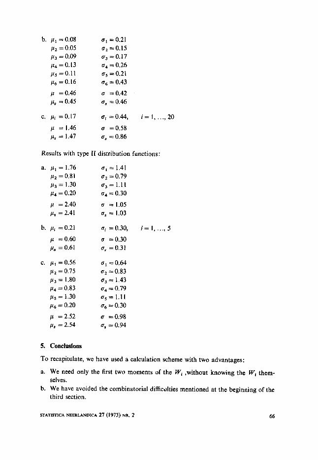
b. pl =0.08 p2 = 0.05 p3 = 0.09 p4 = 0.13 p5 = 0.1 1 c(6 =0.16

p =0.46 ps -0.45

0 1 = 0.21 o2 = 0.15 o3 =0.17 o4 = 0.26

a6 = 0.43

u =0.42 oS = 0.46

6 5 = 0.21

C. pi =0.17 Ui =0.44, i = I , ..., 20

p = 1.46 u =0.58 ps = 1.47 oS =0.86

Results with type I1 distribution functions:

a. pl = 1.76 n1 = 1.41 p2 = 0.81 U~ = 0.79

jl4 = 0.20 u4 = 0.30

p = 2.40 Q = 1.05 ps = 2.41 U, = 1.03

p 3 = 1.30 rJ3 = 1.11

b. pi =0.21 ui =0.30, i = 1, ..., 5

p =0.60 u 10.30 ps =0.61 a, =0.31

c. p , = O . M p2 = 0.75 p 3 = 1.80 p4 = 0.83 ~5 = 1.30 p6 = 0.20

p = 2.52 pcs =2.54

o1 = 0.64 c2 = 0.83

= 1.43 c4 = 0.79 0 5 = 1.1 1

u =0.98 U~ = 0.94

0 6 0.30

5. Conclusions

To recapitulate, we have used a calculation scheme with two advantages:

a. We need only the first two moments of the W , ,without knowing the W , them-

b. We have avoided the combinatorial difficdties mentioned at the beginning of the selves.

third section.

STATISTICA NEERLANDICA 27 (1973) NR. 2 66

It is an unsolved problem why the results from the simulation are so close to those derived from the calculation scheme. One would expect that repeatedly use of our calculation scheme would destroy the approximations, because the scheme can bring us out of the class C.

Acknowledgement

The author wishes to express his thanks to Professor J. W. COHEN for this valuable criticism.

STATISTICA NEERLANDICA 27 (1973) NR. 2 67