the mechanical behaviour of ballasted railway tracks - repository
TRANSCRIPT

The Mechanical Behaviour of Ballasted
Railway Tracks


The Mechanical Behaviour of Ballasted
Railway Tracks
PROEFSCHRIFT
ter verkrijging van de graad van doctoraan de Technische Universiteit Delft,
op gezag van de Rector Magnificus prof. dr. ir. J.T. Fokkema,in het openbaar te verdedigen ten overstaan van een commissie,
door het College voor Promoties aangewezen,op maandag 24 juni 2002 te 16:00 uur
door
Akke Simon Johanna SUIKER
civiel ingenieurgeboren te Venhuizen

Dit proefschrift is goedgekeurd door de promotoren:
Prof. dr. ir. C. Esveld
Prof. dr. ir. R. de Borst
Samenstelling promotiecommissie:
Rector Magnificus, VoorzitterProf. dr. ir. C. Esveld, Technische Universiteit Delft, promotorProf. dr. ir. R. de Borst, Technische Universiteit Delft, promotorProf. dr. R. Chambon, Grenoble Universite Joseph Fourier, FrankrijkProf. C.S. Chang, Ph.D., University of Massachusetts, Verenigde StatenProf. dr. ir. D.J. Rixen, Technische Universiteit DelftProf. E.T. Selig, Ph.D., University of Massachusetts, Verenigde StatenProf. dr. ir. D.H. van Campen, Technische Universiteit Eindhoven
Published and distributed by: DUP Science
DUP Science is an imprint of
Delft University PressP.O. Box 98NL-2600 MG DelftThe NetherlandsTelephone: +31 15 2785678Telefax: +31 15 2785706E-mail: [email protected]
ISBN 90-407-2307-9
Keywords: track dynamics, moving load, track deterioration, laboratory testing, consti-tutive modelling, homogenisation methods
Copyright c© 2002 by A.S.J. Suiker
Cover design by A.S.J. Suiker
All rights reserved. No part of the material protected by this copyright notice may bereproduced or utilized in any form or by any means, electronic or mechanical, includingphotocopying, recording or by any other information storage and retrieval system, with-out written permission from the publisher: Delft University Press.
Printed in The Netherlands

ForewordThe research presented in this thesis was carried out for the main part at the Facultyof Civil Engineering and Geosciences and the Faculty of Aerospace Engineering atDelft University of Technology.I would like to gratefully acknowledge my promotors Coenraad Esveld and Rene
de Borst, for their support, encouragement, and trust during the course of thestudy.In addition, I am indebted to present and former colleagues at the Faculty of
Aerospace Engineering and the Faculty of Civil Engineering of Delft Universityof Technology for their direct and indirect support, and for creating a pleasantand stimulating work environment. In this regard, I particularly would like toacknowledge my former room mates Harm Askes, Otto Heeres and Gideon van Zijl.The experimental research reported in Chapter 5 of this thesis was carried out
at the University of Massachusetts, Amherst, U.S.A., during a research visit fromJanuary 1998 to October 1998. I wish to express my sincere gratitude to Ernest Seligfor inviting me to come to the University of Massachusetts, and to all the peoplethere who made my stay a very pleasant one. I owe many thanks to RaymondFrenkel, for his dedicated assistance during the performance of the experimentalprogram.Furthermore, I would like to direct acknowledgements to Ching Chang (Univer-
sity of Massachusetts), Andrei Metrikine (Russian Academy of Sciences, NizhnyNovgorod, Russia), and Bert Sluys (Delft University of Technology) for the stimu-lating discussions and interactions on wave propagation and homogenisation meth-ods.I am grateful to Adam Fields for perusing the manuscript and correcting the final
linguistic errors.My family and friends, who granted me their support, are also gratefully ac-
knowledged.Finally, I would like to deeply thank Jose, for her support, love and patience.
The birth of our children, Iris and Lennart, has provided the enjoyment that makeslife much more complete.
Akke SuikerDelft, January 2002

Contents
1 Introduction 11.1 Requirements for ballasted tracks . . . . . . . . . . . . . . . . . . . . . . . . . . . 11.2 Track dynamics . . . . . . . . . . . . . . . . . . . . . . . . . . . . . . . . . . . . . . . . 41.3 Future alternatives to ballasted tracks . . . . . . . . . . . . . . . . . . . . . . . 51.4 Modelling aspects . . . . . . . . . . . . . . . . . . . . . . . . . . . . . . . . . . . . . . . 61.5 Objectives and scope . . . . . . . . . . . . . . . . . . . . . . . . . . . . . . . . . . . . 71.6 Outline . . . . . . . . . . . . . . . . . . . . . . . . . . . . . . . . . . . . . . . . . . . . . . . 91.7 Notation . . . . . . . . . . . . . . . . . . . . . . . . . . . . . . . . . . . . . . . . . . . . . . 11
2 Influence of train velocity on track dynamics 132.1 Rail deflection measurements . . . . . . . . . . . . . . . . . . . . . . . . . . . . . . 142.2 Model and governing equations . . . . . . . . . . . . . . . . . . . . . . . . . . . . 152.3 General form of the steady state solution . . . . . . . . . . . . . . . . . . . . . 212.4 Case study . . . . . . . . . . . . . . . . . . . . . . . . . . . . . . . . . . . . . . . . . . . . 27
2.4.1 Timoshenko beam on relatively soft halfspace . . . . . . . . . . . 272.4.2 Timoshenko beam on relatively stiff halfspace . . . . . . . . . . . 35
2.5 Discussion . . . . . . . . . . . . . . . . . . . . . . . . . . . . . . . . . . . . . . . . . . . . . 38
3 Enhanced continua and discrete lattices to model granular media 413.1 Homogenisation of a granular material . . . . . . . . . . . . . . . . . . . . . . . 43
3.1.1 Micro-level particle interaction . . . . . . . . . . . . . . . . . . . . . . . 433.1.2 From micro-level to macro-level . . . . . . . . . . . . . . . . . . . . . . 463.1.3 Macroscopic constitutive formulation . . . . . . . . . . . . . . . . . . 49
3.2 Strain-gradient continua versus discrete Born-Karman lattice . . . . . 533.2.1 Dispersion relation for Born-Karman lattice . . . . . . . . . . . . . 543.2.2 Dispersion relation and stability aspects for strain-gradient
continua . . . . . . . . . . . . . . . . . . . . . . . . . . . . . . . . . . . . . . . . 553.2.3 Discussion of dispersion curves . . . . . . . . . . . . . . . . . . . . . . . 59
3.3 Higher-order continuum that includes particle rotation . . . . . . . . . . 623.4 Strain-gradient micro-polar continuum versus square lattice . . . . . . 70
3.4.1 Dispersion relations for square lattice . . . . . . . . . . . . . . . . . . 713.4.2 Dispersion relations for second-gradient micro-polar contin-
uum and Cosserat continuum . . . . . . . . . . . . . . . . . . . . . . . . 743.4.3 Discussion of dispersion curves . . . . . . . . . . . . . . . . . . . . . . . 77
3.5 Discussion . . . . . . . . . . . . . . . . . . . . . . . . . . . . . . . . . . . . . . . . . . . . . 81
4 Dynamic response of a discrete granular layer 834.1 Governing equations for a square lattice . . . . . . . . . . . . . . . . . . . . . . 85
4.1.1 Lattice model versus continuum model . . . . . . . . . . . . . . . . . 89

viii Contents
4.2 Dispersion curves of the body waves . . . . . . . . . . . . . . . . . . . . . . . . 924.3 Dispersion branches of the layer modes . . . . . . . . . . . . . . . . . . . . . . 96
4.3.1 Variation of particle size . . . . . . . . . . . . . . . . . . . . . . . . . . . . 994.3.2 Variation of layer thickness . . . . . . . . . . . . . . . . . . . . . . . . . . 101
4.4 Formulation and solution procedure of the boundary value problem 1024.4.1 Derivation of steady state displacements . . . . . . . . . . . . . . . . 1024.4.2 Analysis of the kinematic characteristics of radiated waves . 109
4.5 Case study . . . . . . . . . . . . . . . . . . . . . . . . . . . . . . . . . . . . . . . . . . . . 1104.5.1 Steady state response for a layer of small particles (r = 1mm) 1114.5.2 Steady state response for a layer of large particles (r = 25mm) 1144.5.3 Influence of the load velocity . . . . . . . . . . . . . . . . . . . . . . . . . 117
4.6 Discussion . . . . . . . . . . . . . . . . . . . . . . . . . . . . . . . . . . . . . . . . . . . . . 123
5 Static and cyclic triaxial testing of subballast and ballast 1275.1 Triaxial testing of subballast material . . . . . . . . . . . . . . . . . . . . . . . 129
5.1.1 Experimental set-up and test procedure . . . . . . . . . . . . . . . . 1305.1.2 Static triaxial tests . . . . . . . . . . . . . . . . . . . . . . . . . . . . . . . . 1325.1.3 Cyclic triaxial tests . . . . . . . . . . . . . . . . . . . . . . . . . . . . . . . . 135
5.2 Triaxial testing of ballast material . . . . . . . . . . . . . . . . . . . . . . . . . . 1455.2.1 Experimental set-up and test procedure . . . . . . . . . . . . . . . . 1455.2.2 Static triaxial tests . . . . . . . . . . . . . . . . . . . . . . . . . . . . . . . . 1465.2.3 Cyclic triaxial tests . . . . . . . . . . . . . . . . . . . . . . . . . . . . . . . . 151
5.3 Discussion . . . . . . . . . . . . . . . . . . . . . . . . . . . . . . . . . . . . . . . . . . . . . 158
6 Modelling of track deterioration 1616.1 Review of the classical plasticity theory . . . . . . . . . . . . . . . . . . . . . . 1626.2 The response envelope under cyclic loading . . . . . . . . . . . . . . . . . . . 1656.3 Formulation of Cyclic Densification Model . . . . . . . . . . . . . . . . . . . . 168
6.3.1 Magnitude of plastic flow . . . . . . . . . . . . . . . . . . . . . . . . . . . 1686.3.2 Direction of plastic flow . . . . . . . . . . . . . . . . . . . . . . . . . . . . 1736.3.3 Pressure-dependent elastic behaviour . . . . . . . . . . . . . . . . . . 175
6.4 Numerical integration of Cyclic Densification Model . . . . . . . . . . . . 1766.4.1 Update of elastic response . . . . . . . . . . . . . . . . . . . . . . . . . . . 1786.4.2 Consistent tangent operator for elastic response . . . . . . . . . . 1806.4.3 Update of elasto-plastic response . . . . . . . . . . . . . . . . . . . . . 1816.4.4 Consistent tangent operator for elasto-plastic response . . . . . 186
6.5 Model calibration . . . . . . . . . . . . . . . . . . . . . . . . . . . . . . . . . . . . . . . 1886.5.1 Calibration of the elastic model . . . . . . . . . . . . . . . . . . . . . . 1886.5.2 Calibration of the cyclic plastic model . . . . . . . . . . . . . . . . . 190
6.6 Case study . . . . . . . . . . . . . . . . . . . . . . . . . . . . . . . . . . . . . . . . . . . . 195

Contents ix
6.6.1 Initial state . . . . . . . . . . . . . . . . . . . . . . . . . . . . . . . . . . . . . . 1956.6.2 Update at tensile failure regime . . . . . . . . . . . . . . . . . . . . . . 1966.6.3 Modelling aspects and results . . . . . . . . . . . . . . . . . . . . . . . . 200
6.7 Discussion . . . . . . . . . . . . . . . . . . . . . . . . . . . . . . . . . . . . . . . . . . . . . 207
References 211
Appendix 223A Length variations of the springs in a 9-cell square lattice . . . . . . . . . 223
Index 225
Summary 229
Samenvatting 233
Curriculum Vitae 237

x Contents

Chapter 1
Introduction
In railway transport, there is an ongoing demand for performance increase, whichis driven by the need to keep a competitive edge against other means of transporta-tion, such as aircrafts, cars and ships. This calls for high technical and economicalrequirements, as embodied by the quest for higher train velocities, larger transportcapacity, lower energy consumption during transport, greater traveller comfort, bet-ter safety levels and lower maintenance costs. Also, the strong environmental con-sciousness is a paramount factor in deciding what form of transportation to choose,introducing additional requirements regarding noise reduction and minimisation ofemission1. Over the last decades, railway companies have directed attention to mostof the above-mentioned criteria, although their prime interest commonly concernsthe enhancement of the transport capacity per unit time, which can be achieved byincreasing the transport capacity and/or the train velocity.
1.1 Requirements for ballasted tracks
The increase of transport capacity has been stimulated by the growing industrialneed for long-distance freight conveyance, especially in large countries like Aus-tralia, South Africa, China and the United States. Accordingly, these countrieshave been the most progressive in the continuous development and application oflonger and heavier trains. The fact that freight transportation requires consider-ably heavier trains than passenger transportation, can be illustrated by comparisonof the static axle load. The static axle load, which reflects the gravity loading ofthe train, for passenger trains normally does not exceed 170 kN , while for freighttrains it may be in between 250 kN and 350 kN (Esveld, 1989). As a result of
1An electric train itself does not produce emission, but the electricity provided to the trainmay be generated by oil-power stations, gas-power stations or coal-power stations.

2 Chapter 1. Introduction
Figure 1.1 : Deterioration of a railway track.
these high axle loads, freight transportation may cause significant track deterio-ration, see Figure 1.1, in particular when it is operated on relatively light railwaytracks originally intended for passenger transportation.
Deterioration of railway tracks can be reduced by subjecting the individual trackcomponents to specific requirements. In the case of a so-called ballasted railwaytrack, which is the track system worldwide applied the most, the track componentsmay be categorised into two groups (Selig and Waters, 1994). The first group isdesignated as the superstructure, consisting of the rails, the fastening system andthe sleepers, whereas the second group is designated as the substructure, consist-ing of the ballast layer, a possible subballast layer and the subgrade (Figure 1.2).The superstructure thus includes all non-granular components of the railway track,while the substructure includes the granular components. To offer resistance toaxle loads higher than 250 kN , the rails need to be of high strength, jointless andmassive, preferably with a weight larger than 60 kg/m1 (Zongliang, 1993). It isthereby desirable to connect the rails via elastic rail fasteners to pre-stressed orreinforced concrete sleepers, which are more durable than the wooden sleepers tra-ditionally used. The ballast layer, whose main functions are to effectively distributethe trainload and to retain the sleepers in their required position, needs to have anominal thickness larger than 300 mm for providing sufficient resiliency, strengthand energy absorption (Zongliang, 1993). These structural demands, however, havenot yet led to a general consensus about adequate requirements for the ballast ma-

1.1 Requirements for ballasted tracks 3
b > 300 mm
s > 150 mm
Recommendation :
BallastSubballast
Subgrade
bs
RailSleeper
Figure 1.2 : Schematised cross-section of a ballasted railway track.
terial index characteristics, such as particle size, particle shape, abrasion resistanceand composition. Instead, the choice of a ballast material is commonly predicatedupon economic considerations and availability, where an extended variety of mate-rials is used, such as crushed granite, limestone, slag, and gravel (Selig and Waters,1994). In addition to structural requirements, the ballast must absorb airbornenoise, it must warrant a proper electrical resistance between the rails, it needs toresist plant growth and must have a high enough drainage capacity. The latter twoobjectives can be properly met by using a ballast grading with particles between15 mm and 80 mm.
A subballast layer is constructed occasionally to further improve the drainagecapacity of the track, as well as to enlarge the train load distribution, to preventtrack upheaval by frost and to avoid penetration and attrition of the ballast par-ticles by the subgrade material. The subballast layer needs to have a nominalthickness of at least 150 mm, to admit for construction variability and for progres-sive settlements under repetitive train loading. A relatively inexpensive materialthat usually serves the above purposes satisfactory is a mixture of sand and finegravel, with grain-sizes between 0.05 mm and 20 mm. Nevertheless, under specificcircumstances it may be necessary to utilise more advanced (and thus more ex-pensive) subballast structures, such as structures of asphalt concrete, geo-syntheticmaterials or cement/lime stabilised soils (Selig and Waters, 1994). The applicationof such improvements strongly depends on the strength and stiffness conditions ofthe subgrade below. The subgrade, which is represented by a natural groundformation or a placed soil fill, may have a relatively low stiffness and/or strength,in the case of which an advanced subballast structure should be prescribed in orderto avoid excessive track deterioration.

4 Chapter 1. Introduction
1.2 Track dynamics
Apart from the magnitude of the static axle load, reflecting the gravity loading ofthe train, the amount of track deterioration is determined by the dynamic loadingcaused by the train-track interaction. Here, several sources of track vibrations canbe distinguished, which are (i) inhomogeneities at the wheel-rail contact, i.e. railirregularities or wheel flats, (ii) inhomogeneities in the track structure, i.e. thesleeper distance, the discrete nature of the ballast, differential settlements, stiffnesstransitions in the subgrade or at bridges, tunnels and (iii) the velocity effect of thetrain. Especially in high-speed railway lines, where train velocities of 200 km/h andhigher are applied, the track response may have a strongly dynamic character thatcan result in significant track deterioration if no structural precautions are taken.This became very clear during the establishment of the 1955 world speed record of331 km/h in France, involving severe track damage due to which the train camedangerously close to derailment (TGV-web, 2000).For recently-built high-speed lines, railway engineers have attempted to reduce
track deterioration by employing specific structural provisions, such as foundationsof concrete and tarmac to warrant a solid support for the ballast layer, the use ofanti-vibration mats to dissipate the vibration energy conducted by the ballast layer,and the application of new damping materials to reduce the high frequency forcecomponents that are transmitted by the rail. Additionally, stringent requirementsare put towards the mechanical preparation of the ballast layer and the admissiblegeometrical tolerances of the track (Esveld, 1989; TGV-web, 2000). This, togetherwith the development of a newer generation of equipment, made it possible to fur-ther increase train speeds, leading to a striking world speed record of 407 km/hin 1988 by a German ICE-train. Driven by competition, in 1990 this speed recordwas improved to 515 km/h by a French TGV-train. Both record runs were estab-lished on newly-built ballasted tracks, specially constructed for high-speed trains.Although the speed records were accomplished without the generation of significantinstantaneous track damage, the wave radiation in the track as well as in the cate-nary system transmitting the electric current appeared to be exceptionally strong(Triantafyllidis and Prange, 1994; TGV-web, 2000). Hence, from the aspects ofperiodical track maintenance and passenger safety, such speeds are not (yet) viablefor commercial service.It is currently believed that the maximum service speed for operational high-
speed railway transport by conventional trains2 is 350 to 400 km/h. Nowadays, forhigh-speed lines in France, Japan, and Spain, service speeds of up to 300 km/h aremaintained, which is already close to the maximum attainable speed for commercial
2The term ’conventional trains’ is used for train vehicles that propagate by means of wheel-railcontact.

1.3 Future alternatives to ballasted tracks 5
service. High speed railway systems in Germany (280 km/h), Italy (250 km/h),Finland (220 km/h), and Sweden, the United Kingdom, Russia and the UnitedStates (200 km/h) are further from this target speed.
Apart from using tracks specially constructed for high-speed railway transport,high-speed trains regularly use the existing railway infrastructure. The main ben-efit thereby is an enormous cost-reduction, as the construction of new high-speedrailway tracks with all their necessary facilities often is prohibitively expensive.There is nevertheless strong evidence that existing railway tracks are not alwayscapable of adequately bearing the increased dynamic loading generated by high-speed trains. In-situ rail deflection measurements have revealed a significant growthof track deformations under an increasing train velocity, especially when the localsubgrade consists of relatively soft soil layers, such as peat or clay layers (Hunt,1994; Madshus and Kaynia, 2000). As a result, at various railway lines in Europespeed restrictions have been established at soft soil locations, thus increasing thetransportation time on these lines.
1.3 Future alternatives to ballasted tracks
Since the settlement behaviour of ballast makes a ballasted track relatively main-tenance intensive, railway engineers are currently increasingly interested in alter-native, non-ballasted track systems. A non-conventional railway system that has alarge potential for future application is the magnetically levitated train (commonlyabbreviated to ’Maglev-train’). For this railway system, frictional contact betweenthe trainwheel and the rail is avoided by applying a magnetic field that levitates thetrain to a distance of 10 centimeters above the track. The magnetic field is gener-ated by using superconducting magnet coils, which are made of very thin wires of aniobium-titanium alloy that are brought into copper-wires (van Kooij, 2000). Thesuperconductivity of these magnet coils is warranted by a cooling-down process, forwhich purpose liquid helium of −269o C is utilised. The magnet coils are installedboth in the train and along the track, where the levitation and movement of thetrain occurs in accordance with the ’stator-rotor principle’ also employed in a ro-tating electro-motor. In combination with superconductivity, this technique makesit possible to achieve train speeds that are higher than those on a conventionalrailway track. In 1997, at a 42.8 km test track in Yamanashi, Japan, a Maglevtrain established a new world speed record of 550 km/h (van Kooij, 2000). De-spite of the speed increase, the very low level of noise and vibrations, and the lowmaintenance, the costs of this type of railway system are significantly higher thanthose of a conventional railway system. Moreover, as yet substantial research effortregarding the long-term reliability and feasibility of the train and track components

6 Chapter 1. Introduction
is necessary before this system can be applied for commercial service.
A non-ballasted track system that nowadays is subject of an increasing popularityis the so-called slab track. In a slab track the load-carrying capacity is fulfilled byreinforced or pre-stressed concrete slabs, which rest on a sand bed and support therails above via directly attached concrete sleepers or via a cast embedment of rubberor cork. The main benefits of this type of structure are its relatively low structuralweight and height, and its high resistance against lateral loading. Furthermore,maintenance costs are relatively low if the structure has sufficient strength andresiliency to prevent cracking of the concrete (Esveld, 2001). The drawbacks ofslab track in regard to ballasted track are the higher construction costs, and thetime-consuming structural precautions that have to be taken to avoid differentialsettlements and cracking of the slabs. These negative issues have thus far preventedwidespread usage of slab track on commercial railway lines (Esveld, 2001). However,increasingly positive experiences with slab track in countries like Germany, Japan,France and The Netherlands can mitigate these drawbacks, which in the near futuremay result in slab track becoming a serious competitor to ballasted track.
1.4 Modelling aspects
Despite of the immense annual funds utilised for construction and maintenance ofrailway tracks, track design and maintenance planning to date still has a stronglyempirical character, with a trial and error basis for decisions. Such a method isopen to faults and misjudgments, due to the time necessary to experience the out-come of trials, an insufficient or inadequate database of historical track records, orthe changing technical and economical requirements over the years. To make thedecision-making procedures regarding track design and maintenance more time andcost effective, it is necessary to thoroughly study and understand the mechanicalprocesses that form the basis of track performance and track deterioration. Thesemechanical processes can be separated into two categories, namely (i) short-termmechanical processes and (ii) long-term mechanical processes. The first categoryembraces the instantaneous, dynamic behaviour of a railway track, as activatedduring the passage of one, or a few, train axles. The permanent track deforma-tions generated during an individual train axle passage are usually very small, suchthat the track behaviour may be viewed as reversible, and thus can be studied bymeans of (visco)elastic models. The viscosity thereby is a measure for the energydissipated during the reversible response. The second category embraces the me-chanical processes characterised by a typically quasi-static time-dependency, suchas track deformations caused by ground water flow or creep processes in clay orpeat layers, track deterioration due to subgrade particle migration into the ballast
1.5 Objectives and scope 7
layer, or long-term substructural settlements and long-term abrasion of rail profilesunder a (very) large number of train axle passages. For all these phenomena, thegenerated permanent deformations may become substantial, which requires the useof (non-linear) plasticity-based or damage-based models to study them.
A separation into short-term mechanical processes and long-term mechanicalprocesses is convenient from the modelling point of view, though for a proper as-sessment of the overall track performance the interaction between these processesshould be also taken into account. For example, a change in track alignment causedby a long-term deterioration process alters the short-term interaction between trainvehicle and track, and vice versa. A way to integrate these short-term processesand long-term processes into one modelling procedure, is to translate the dynamicresponse to an instantaneous train axle passage into one or more dynamic amplifi-cation factors, which may serve as multipliers for the quasi-static loading appliedin the simulation of long-term track deterioration. Conversely, the settlement pro-file computed in a simulation of long-term track deterioration can serve as inputfor a dynamic analysis of the instantaneous vehicle-track interaction. If during aspecific time interval the mutual influence between a long-term mechanical processand a short term mechanical process is accounted for more frequently, the overalltrack performance will be simulated more accurately. Notwithstanding, the actualnumber of stages at which the mutual influence is considered should be based on aproper compromise between model accuracy and computational economy.
1.5 Objectives and scope
The overall objective of this thesis is to develop advanced models that providedetailed insight into important short-term and long-term mechanical processes in arailway track. The study will be confined to ballasted railway tracks, although inseveral cases the methodology presented can also be applied to other track systems.The short-term mechanical processes to be studied concern the wave propagationactivated in a railway track by a moving train axle. Attention will be focused onthe growth of the track response due to an increasing train velocity, the effect ofwhich serves as an important criterion for the design of high-speed railway lines.In-situ track measurements have demonstrated that surface waves initiated by atrain may cause a resonance-like phenomenon in the railway system, which becomesmanifest when the train reaches a characteristic critical velocity. From the aspectsof passenger safety and track deterioration control it is very important to scrutiniseand understand this phenomenon in all its details.
Apart from the characteristics of generated waves being dependent on the ve-locity effect of the train, they also depend on inhomogeneities present in the track

8 Chapter 1. Introduction
system, such as the discrete nature of the ballast particles, the discrete sleepersupport, stiffness transitions, and irregularities at the rail surface and train wheelsurface. Track inhomogeneities especially modify those waves of which the wave-length is similar to the characteristic length of the inhomogeneity, i.e. waves witha wavelength approximately equal to the ballast particle size, the sleeper distance,the length of the stiffness transition or the size of a rail or wheel irregularity. Inorder to examine the effect of these relatively short waves, it is necessary to includethe characteristic length of interest into the model to be used. In the case of the bal-last particle size, this can be done by employing a so-called kinematically-enhancedcontinuum model that considers the ballast particle size as an explicit materialparameter, or by using a discrete lattice model in which the ballast particle sizecorresponds to the distance between the individual discrete masses. It is one ofthe purposes of this study to derive enhanced continuum models from the discretemicro-structure of a granular material, which can be done by applying homogeni-sation techniques. It is thereby important to reveal the accuracy level at which thediscrete granular behaviour is approximated by the continuum model, for exampleby means of a comparison with corresponding discrete lattice models. Furthermore,the derived enhanced continuum models need to be examined on their suitabilityfor application in engineering problems, which depends on stability and uniquenesscharacteristics, and the simplicity of the boundary conditions. The present studyaims to give insight into these issues.
The question as to whether or not a ballast layer should be modelled by a con-tinuum model or a discrete model is essential, both from a computational point ofview and from a physical point of view. As far as the former aspect is concerned,a discrete model generally requires more material points to be evaluated than acontinuum model, and thus requires more computational effort to solve the cor-responding system of equations. This may be the reason that railway engineersoften prefer to use continuum models to study the mechanical behaviour of bal-last. As far as the latter aspect is concerned, the choice for a continuum modelor a discrete model is less evident. In fact, this depends on the characteristics ofthe inhomogeneous deformation patterns emerging in the ballast layer, which aregoverned by various factors, such as the loading conditions, the internal materialstructure of the ballast, and the structural geometry of the track. The intention ofthis thesis is to exhibit how, and up to which intensity level, such factors perturbthe discrete nature of a ballast layer. This will be done by means of a comparativestudy regarding the response of a discrete layer and a continuous layer to a moving,harmonically vibrating (axle) load.
For reasons of simplicity, the boundary value problems treated in the study ofwave propagation will be two-dimensional, in a sense that they only consider thevertical geometry plane in the longitudinal direction of the track. Although in a

1.6 Outline 9
two-dimensional model the geometrical radiation of waves is different from thatin a (more realistic) three-dimensional model, in a qualitative sense the dynamicbehaviour of two- and three-dimensional models here is similar, since this is mainlydetermined by the response characteristics in the directions of loading and loadpropagation.
The long-term mechanical process that will be studied in this thesis concerns theevolution of track deterioration as a result of a large number of train axle passages.In a ballasted railway track, track deterioration is formed for the main part by theplastic deformations generated in the granular substructure. Since track settlementprofiles commonly have wavelengths that are much larger than the particle sizesof the substructural components, it is allowed to model track deterioration withinthe notion of a (standard) continuum theory. By implementing the continuummodel into a finite element code, it should be possible to numerically simulate thenon-linear accumulation of track deformations developing under a large numberof train axle passages (or load cycles). In this respect, a model that describes thecomplete response during each individual load cycle is regarded as unsuitable, sincesuch a model requires a (very) large amount of computational effort to simulate thestructural behaviour during common track deterioration periods. It is one of theaims of this work to develop a more efficient cyclic model. The calibration of thecyclic model will be carried out by using experimental data obtained from staticand cyclic triaxial tests on a ballast and subballast material.
1.6 Outline
The thesis commences with a study of the effect of the train velocity on the dy-namic response of a railway track. Hereto, a Timoshenko beam supported by ahalfspace is subjected to a moving load. The Timoshenko beam represents thecompound system of rails, sleepers and ballast, whereas the halfspace representsthe subgrade underneath. The moving load is representative for a moving trainaxle. The response characteristics around critical load velocities are investigatedby means of a finite element study, and compared to the response characteristicsobtained from in-situ measurements. Furthermore, it is demonstrated how to re-trieve these critical velocities (which serve as a useful design parameter) from amore simple, kinematic analysis.
Chapter 3 focuses on the modelling of the inhomogeneous nature of coarse gran-ular materials, such as ballast. The derivation of several elastic, kinematically-enhanced continuum models from the discrete micro-structure of a granular mediumis treated. The homogenisation framework employed distinguishes the influence ofstrain (-gradient) terms and rotation (-gradient) terms. To reveal accuracy, unique-

10 Chapter 1. Introduction
ness and stability aspects of the continuum models, their dynamic characteristicsare compared to those of corresponding discrete lattice models, which is done byperforming dispersion analyses.
In Chapter 4 the dynamic response of a ballast layer to an instantaneous train axlepassage is simulated, by employing a discrete lattice model subjected to a moving,harmonically vibrating load. The frequency of the harmonic load is set equal to thesleeper passing frequency, since the sleeper passing effect generally is considered tobe a prominent source of track vibrations. The response characteristics computedare compared with the response characteristics of a corresponding continuummodel,such that within the context presented it becomes obvious what the main differencesbetween these two types of modelling are. Within the frames of the comparison,the effect on the layer response by the axle load velocity, the load frequency, theparticle size, the layer thickness, and the material damping is exemplified.
The above chapters solely address short-term mechanical processes in a railwaytrack, where a global distinction can be made between dynamic response charac-teristics corresponding to relatively long waves (Chapter 2) and dynamic responsecharacteristics corresponding to relatively short waves (Chapters 3 and 4). In Chap-ter 5, the attention is shifted towards long-term mechanical processes, by consider-ing cyclic triaxial tests that provide the response characteristics of a ballast and asubballast material under a large number of load cycles. The experimental set-up,the test procedure and the test results are treated. The test results both exhibitthe elastic deformation behaviour and the permanent deformation behaviour of theballast and subballast material considered. In addition to the cyclic triaxial tests,static triaxial tests are treated. The static tests were carried out to provide themaximum stress level that can be applied in the cyclic tests, and to demonstratethe increase in material strength and material stiffness as a result of the cyclicloading process. The test results are used for the calibration of the Cyclic Densi-fication Model proposed in Chapter 6. The Cyclic Densification Model describesthe envelope of the irreversible, plastic material response generated during a cyclicloading process, thereby distinguishing between the mechanisms of frictional slidingand volumetric compaction. The reversible response is represented by a pressure-dependent, hypo-elastic material law. The numerical integration procedure of theconstitutive model is specified, after which the model is employed in a (finite ele-ment) case study regarding the long-term settlement behaviour of a railway track.The main features of the model are illustrated by comparing the long-term cyclicresponse computed to the long-term cyclic response obtained from in-situ trackmeasurements.
It is acknowledged that the various subjects treated in this thesis may not be allof the same level of interest for readers with a specific interest or background. Tomake readers easily find their subject of interest, the following global categorisa-
1.7 Notation 11
tion may be helpful: wave propagation due to moving loads (Chapters 2 and 4),homogenisation techniques for granular materials (Chapter 3), laboratory testingof granular materials (Chapter 5), elasto-plastic modelling of granular materials(Chapter 6), and numerical implementation of constitutive models (Chapter 6).Further, at the end of each chapter, the main conclusions and results of the chapterhave been summarised and translated towards (railway) practice.
1.7 Notation
When the theoretical concept of a model is treated, tensor notation is used. Whenthe numerical integration procedure of a model is discussed, matrix vector notationis used. Here, matrices are designated by bold uppercase symbols and vectors aredesignated by bold lowercase symbols. Symbols are defined the first time theyappear in the text. Although care has been taken to avoid conflict in notation, ina very few cases a symbol may have more than one meaning. The meaning of asymbol can be inferred from the context within which it is introduced.

12 Chapter 1. Introduction

Chapter 2
Influence of train velocity ontrack dynamics
In order to meet the high standards regarding effectiveness of railway transporta-tion, in numerous countries train cruising speeds of 200 km/h and higher havealready been applied or will be applied in the near future. Such high speeds causethe response of the railway track to have a dynamic character. In general, the signa-ture of the dynamic response is determined by a combination of the train velocity,the axle distance, and structural inhomogeneities in the train-track system, suchas wheel flats, rail irregularities, the sleeper distance and differential settlements.Nevertheless, rail deflection measurements at high-speed railway tracks in France(Fortin, 1982), Great Britain (Hunt, 1994) and Sweden (Madshus and Kaynia, 2000)provided response patterns that are mainly affected by the train velocity, and notso much by the axle distance and the train-track inhomogeneities. It appeared thatthe growth of this dynamic amplification can already become significantly largein the range of commercial train speeds, especially when the subgrade consists ofrelatively soft materials, such as clay or peat (Hunt, 1994; Madshus and Kaynia,2000).
In the beginning of the 1990’s, in the field of railway engineering it was roughlyunderstood that velocity-dependent track amplifications originate from accumula-tion of surface wave energy under the train wheels. This resonance-like phenomenonhad been identified some decades before, by means of theoretical studies on a beam-halfspace configuration subjected to a moving load (Fillipov, 1961; Labra, 1975).The beam thereby represents the combined rail-sleeper-ballast system, the halfspacerepresents the natural subgrade, and the moving load simulates the movement ofan individual train axle. Notwithstanding, the extended construction of high-speedlines during the last decade required more insight into the velocity-dependency ofthe track response, as strongly impelled from passenger safety criteria and track
14 Chapter 2. Influence of train velocity on track dynamics
deterioration control. This incited investigators to further develop and analysebeam-halfspace models subjected to moving loads, both in an analytical mannerand in a numerical manner (Dieterman and Metrikine, 1997b; Suiker et al., 1998;Lieb and Sudret, 1998; Kaynia et al., 2000; Kononov and Wolfert, 2000). All thesemodels are constructed within the theory of classic linear elasticity. The choicefor an elastic formulation, however, is reasonable, since the track response duringan individual load passage is mainly reversible. Furthermore, the complexity ofmoving load problems commonly urges the usage of linear models, which to someextent may lead to deviations if the response amplitude becomes relatively large.In this chapter, the moving load model presented in Suiker et al. (1998) is dis-
cussed. The configuration consists of a Timoshenko beam that is connected to atwo-dimensional halfspace by means of an interface. After a preliminary discus-sion of rail deflection measurements in high-speed railway tracks, the mathematicalframework describing the steady-state response of this beam-halfspace system isderived. The steady-state solution is used to perform a kinematic analysis thatprovides the frequencies and the wavenumbers of the interface waves radiated bythe load. The kinematic analysis is further employed to find the so-called criti-cal velocities of the system, which are the load velocities that cause the waves inthe beam-halfspace system to resonate. Subsequently, a finite element analysis iscarried out in which an accelerating load passes the resonance states of the beam-halfspace system. The computed response is explained by using the results fromthe kinematic analysis. The response characteristics of the model are also validatedto in-situ measurements in high-speed railway tracks.
2.1 Rail deflection measurements
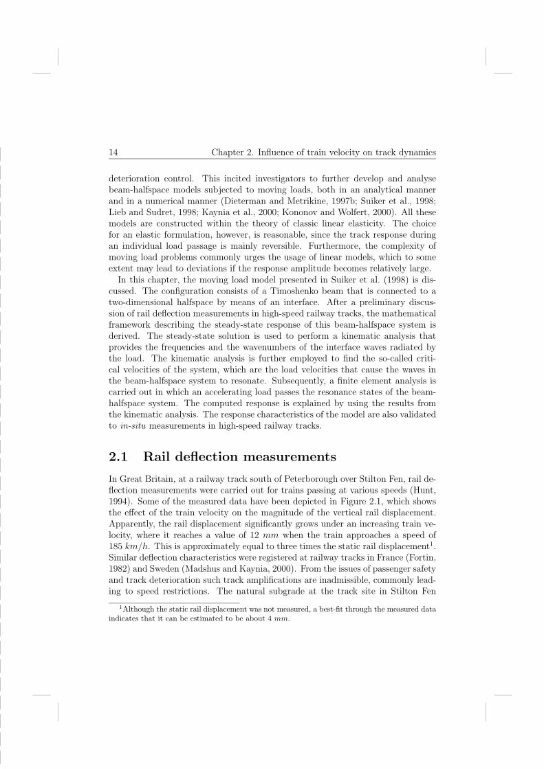
In Great Britain, at a railway track south of Peterborough over Stilton Fen, rail de-flection measurements were carried out for trains passing at various speeds (Hunt,1994). Some of the measured data have been depicted in Figure 2.1, which showsthe effect of the train velocity on the magnitude of the vertical rail displacement.Apparently, the rail displacement significantly grows under an increasing train ve-locity, where it reaches a value of 12 mm when the train approaches a speed of185 km/h. This is approximately equal to three times the static rail displacement1.Similar deflection characteristics were registered at railway tracks in France (Fortin,1982) and Sweden (Madshus and Kaynia, 2000). From the issues of passenger safetyand track deterioration such track amplifications are inadmissible, commonly lead-ing to speed restrictions. The natural subgrade at the track site in Stilton Fen
1Although the static rail displacement was not measured, a best-fit through the measured dataindicates that it can be estimated to be about 4 mm.

2.2 Model and governing equations 15
Train velocity [km/hour]
120 130 140 150 160 170 180 190 200
Ve
rtic
al ra
il d
isp
lace
me
nt
[m
m]
4
5
6
7
8
9
10
11
12
13
14
Train type : Electra. 91
Train type : High-speed
Best fit
Figure 2.1: Vertical rail displacement at different train velocities, measured at StiltonFen, England, January-May 1993. Reprinted from Hunt (1994), with kind permission ofUnion Railways Limited, London.
consists of peat with some clay, having a depth of about 7 m. The soft subgradematerial is believed to play a very important role in the dynamic amplificationof the track response. This will be analysed in the current chapter by means ofscrutinising a beam-halfspace configuration subjected to a moving load.
2.2 Model and governing equations
Figure 2.2 depicts a configuration of a Timoshenko beam with height Hb that isconnected to a halfspace via an interface. The configuration is subjected to amoving, harmonically vibrating load that simulates a moving train axle. Here, Fz
is the magnitude of the load, Ω is the load frequency, vx is the load velocity inthe x-direction, t is time, i2 = −1 is trivial, and δ(..) is the well-known Diracdelta function. The beam models the bending (M) and shearing (Q) behaviour ofthe compound system of rails, sleepers, ballast and subballast, while the halfspaceconstitutes the natural subgrade. The beam-halfspace interaction is described byinterface tractions in the normal direction tn and the tangential direction tt. Thesubgrade can be either stiffer than the track system, for example rock, or softerthan the track system, for example clay, peat or sand.For an arbitrary material point in the halfspace, the relation between the stress

16 Chapter 2. Influence of train velocity on track dynamics
exp(i δ
b
t) (x - v t)Ω x
vx
zF
Halfspace
Interface
z, w
Q
Q+dQ
Timoshenko beamH
x
φ
tt
tt
nt
M+dMM
nt
Figure 2.2: Moving harmonically vibrating load on a Timoshenko beam that is con-nected to a half space by means of an interface. The internal equilibrium of the beam isdefined by the shear force Q, the bending moment M , and the interface tractions in thenormal direction tn and the tangential direction tt.
tensor σij and the strain tensor εij may be formulated as
σij = Dijkl εkl with i, j, k, l ∈ x, y, z, (2.1)
where, under the assumption of a homogeneous isotropic elastic medium, the con-stitutive tensor Dijkl equals
Dijkl = λδijδkl + µ (δikδjl + δilδjk) . (2.2)
Here, λ and µ are the Lame constants and δij is the Kronecker delta,
δij =
1 if i = j0 if i = j
. (2.3)
When considering small displacement gradients, the strain tensor εij may be ap-proximated by the symmetric part of the first-order gradient of the displacementfield,
εij =1
2(ui,j + uj,i) , (2.4)
where ui is the displacement and , j denotes the spatial derivative in the j-th di-rection. Substituting Eq.(2.2) into Eq.(2.1), and using the fact that Eq.(2.4) issymmetric, yields the well-known form
σij = λδijεkk + 2µεij. (2.5)

2.2 Model and governing equations 17
In addition to the constitutive relation (2.5) and the kinematic relation (2.4), thelocal form of the conservation of linear momentum is formulated as
ρ ui,tt = σji,j + ρbi , (2.6)
in which , t designates the time derivative, ρ is the mass density, and bi is thebody force per unit mass. Further, a repetition of spatial derivatives j implies asummation. By virtue of the principle of conservation of angular momentum andassuming that couple stresses and/or body couples are absent, the stress tensor in(2.6) will be symmetric, i.e. σij = σji. Under these conditions, the stress tensor isknown as the symmetric Cauchy stress, whereas the continuum in which this stresssymmetry holds is called a Boltzmann continuum2. When combining Eqs.(2.4),(2.5) and (2.6) in a straightforward manner, the equations of motion are obtainedas
ρ ui,tt = (λ+ µ)uj,ij + µui,jj , (2.7)
where it is assumed that the body force contribution ρbi may be neglected. In-voking the Helmholtz decomposition, the displacement field can be expressed in thefollowing form (see for example, Ewing et al., 1957; Achenbach, 1973)
ui = Φ,i + eijkΨk,j with Ψk,k = 0, (2.8)
where Φ is a scalar potential representing the irrotational part of the displacementfield, and Ψk is a vector potential representing the equivoluminal part of the dis-placement field. Substituting the decomposition (2.8) into (2.7) results in
ρ[Φ,itt + eijk Ψk,jtt] = (λ+ µ)[Φ,ijj + eijk Ψi,kij] + µ[Φ,ijj + eijk Ψk,jjj], (2.9)
with eijk the permutation symbol, such that
eijk =
+1 if ijk represents an even permutation xyz0 if any two of the ijk indices are equal
−1 if ijk represents an odd permutation of xyz. (2.10)
Reordering Eq.(2.9) and invoking the requirement Ψk,k = 0 presented in Eq.(2.8)3
yields[ρΦ,tt − (λ+ 2µ)Φ,jj],i + eijk[ρ Ψk,tt − µΨk,jj],j = 0. (2.11)
2 In the class of micro-polar continua, couple stresses and/or body couples do appear as a resultof the enhancement of the kinematic field with rotational degrees of freedom. Consequently, in amicro-polar continuum the Cauchy stress is non-symmetric.
3The introduction of the constraint Ψk,k = 0 in Eq.(2.8) is necessary for reducing the totalnumber of independent components of the potentials Φ and Ψi from four to three, in agreementwith the three components of the displacement vector ui. Although other choices for the constraintcondition are possible, the advantage of the current constraint is that it leads to an elegantmathematical formulation for the elasto-dynamic problem.

18 Chapter 2. Influence of train velocity on track dynamics
According to this expression, the displacement decomposition (2.8) satisfies theequations of motion (2.7) if the potentials Φ and Ψi are solutions of the equations
Φ,tt = (cP )2 Φ,jj (2.12)
andΨi,tt = (cS)2 Ψi,jj , (2.13)
in which cP and cS are the compression wave velocity and the shear wave velocity,respectively, given by
cP =
√λ+ 2µ
ρ
cS =
õ
ρ.
(2.14)
The Helmholtz equations (2.12) and (2.13) are better known as the wave equa-tions, describing the propagation of the compression wave and the shear wave,respectively. Despite of the potentials Φ and Ψi commonly being coupled by meansof boundary conditions, the decomposition (2.8) may diminish the complexity ofthe elasto-dynamic analysis4. For a detailed discussion on the uniqueness of theHelmholtz decomposition, the reader is referred to Achenbach (1973).Within the frames of linear elastic wave propagation in homogeneous, isotropic
media, a Helmholtz decomposition of the displacement field leads to two indepen-dent wave equations for arbitrary wave types. The most elementary wave type isthe plane wave, since any other wave type, such as the cylindrical wave or the spher-ical wave, can be constructed as a superposition of plane waves. For plane wavepropagation in an orthonormal x-z plane, the spatial derivatives in the y-directiondisappear, which turns Eq.(2.8) into
ux = Φ,x − Ψy,z
uy = Ψx,z − Ψz,x
uz = Φ,z + Ψy,x .
(2.15)
Here, Φ represents the propagation of the compression wave (P-wave) in the x-zplane, Ψy represents the propagation of the vertically polarised shear wave (SV-wave) in the x-z plane, and Ψx and Ψz describe the propagation of the horizontally
4For media more complicated than the homogeneous isotropic medium, a decomposition of thedisplacement field into potentials not necessarily improves the elegance and convenience of thesolution procedure, under which circumstances their introduction should be contemplated withgreat care.

2.2 Model and governing equations 19
polarised shear wave (SH-wave) that corresponds to a shear motion perpendicularto the x-z plane. As a result of decomposing the shear wave into two orthogonaltypes of shear motion, the combined P-SV-wave propagation is uncoupled from theSH-wave propagation.When assuming the configuration in Figure 2.2 as ’plane strain’, the displace-
ment in the y-direction, Eq.(2.15-b), vanishes. Correspondingly, the wave equations(2.12) and (2.13) reduce to
Φ,tt = (cP )2 (Φ,xx + Φ,zz)
Ψy,tt = (cS)2 (Ψy,xx + Ψy,zz) .(2.16)
Furthermore, a combination of Eqs.(2.4), (2.5), (2.15-a) and (2.15-c) yields thefollowing relations for the stresses σzz and σzx in terms of the potentials Φ and Ψy
σzz = λ∇2Φ+ 2µ (Φ,zz + Ψy,xz)
σzx = µ (2Φ,xz + Ψy,xx − Ψy,zz) ,(2.17)
with the scalar operator ∇2(..) = (..),xx + (..),zz. At the interface z = 0 the Timo-shenko beam is connected to the halfspace. Requiring traction equilibrium at theinterface yields
σzz
∣∣∣z=0
= −tn
σzx
∣∣∣z=0
= tt ,(2.18)
with tn the traction in the normal direction of the interface and tt the traction inthe tangential direction of the interface. The equations of motion for the Timo-shenko beam, which include the contribution of the uniformly moving, harmonicallyvibrating load, Fz exp(iΩt) δ(x − vxt), can be expressed as
ρbAb w,tt = Q,x − tn + Fz exp(iΩt) δ(x− vxt)
ρbIb φ,tt = −Q+M,x +12Hbtt .
(2.19)
Here, Ab is the beam cross section per unit length, Ib is the beam moment of inertiaper unit length, ρb is the density of the beam, w is the vertical beam displacement, φis the beam rotation, Q is the shear force in the beam, M is the bending moment inthe beam and 1/2Hb designates the distance between the neutral axis of the beamand the interface, in correspondence with a total beam height Hb. The shearingangle of the Timoshenko beam γ is defined by (see for example, Achenbach, 1973)
γ = w,x + φ, (2.20)

20 Chapter 2. Influence of train velocity on track dynamics
which enables to formulate a constitutive relation for both the shear behaviour andthe bending behaviour of the beam,
Q = η µbAb γ
M = EbIb φ,x ,(2.21)
with µb and Eb the shear modulus and the bending modulus of the beam, respec-tively, and η a factor taking into account the non-uniform shear distribution overthe beam cross section Ab. The equations of motion in terms of beam displace-ments and halfspace potentials follow from inserting Eq.(2.17) into Eq.(2.18), andsubsequently substituting Eqs.(2.18), (2.20) and (2.21) into Eq.(2.19),
ρbAbw,tt = ηµbAb (w,x + φ),x + λ∇2Φ+ 2µ (Φ,zz + Ψy,xz) + Fz exp(iΩt) δ(x− vxt)∣∣∣z=0
ρbIbφ,tt = − ηµbAb (w,x + φ) + EbIbφ,xx + 12H
bµb (2Φ,xz + Ψy,xx − Ψy,zz)∣∣∣z=0
,
(2.22)where the denotation (..)|z=0 indicates that the complete expression preceding thissymbol is considered at the beam-halfspace interface z = 0. Now that the equationsof motion have been derived, the next step is to formulate the transitional conditionsat the interface between the beam and the halfspace. The interface displacementsin the normal direction and the tangential direction, ∆un and ∆ut, can be relatedto beam degrees of freedom and halfspace degrees of freedom as
∆un = uz − w∣∣∣z=0
∆ut = ux − 12Hbφ
∣∣∣z=0
.(2.23)
In addition, the constitutive relation of the interface is
tn = Dnn ∆un +Dnt ∆ut
tt = Dtn ∆un +Dtt ∆ut ,(2.24)
where Dnn is the interface stiffness in the normal direction, Dtt is the interfacestiffness in the tangential direction, and Dnt and Dtn are the stiffnesses couplingthe constitutive behaviour in the normal direction to that in the tangential direc-tion, and vice versa. For simplicity reasons, the influence of the coupling termsis neglected, i.e. Dnt = 0, Dtn = 0. Furthermore, the interface stiffness Dnn isconsidered to be infinitely large, which embodies a ’rigid’ connection in the normaldirection. Correspondingly, a combination of Eq.(2.23) and Eq.(2.24) yields
uz
∣∣∣z=0
= w
tt = Dtt
(uz − 1
2Hbφ
) ∣∣∣z=0
,(2.25)

2.3 General form of the steady state solution 21
which, after successively invoking (2.18-b), (2.17-b) and (2.15), gives
Φ,z + Ψy,x
∣∣∣z=0
= w
µ (2Φ,xz + Ψy,xx − Ψy,zz)∣∣∣z=0
= Dtt
(Φ,x − Ψy,z − 1
2Hbφ
) ∣∣∣z=0
.(2.26)
With Eqs.(2.26), (2.22) and (2.16), a mathematical framework has been constructedthat describes the elasto-dynamics of the beam-halfspace system under a movingload. In the next section, the expressions for the steady state solution of this systemwill be derived.
2.3 General form of the steady state solution
In order to compute the steady state response of the beam-halfspace system to amoving load, Fourier integral transformations with respect to time t and the x-coordinate are applied to the beam degrees of freedom w and φ and the halfspacepotentials Φ and Ψy,
˜w(kx, ω) =
∫ ∞
−∞
∫ ∞
−∞w(x, t) exp
(i(kxx− ωt)
)dx dt
˜φ(kx, ω) =
∫ ∞
−∞
∫ ∞
−∞φ(x, t) exp
(i(kxx− ωt)
)dx dt
˜Φ(kx, z, ω) =
∫ ∞
−∞
∫ ∞
−∞Φ(x, z, t) exp
(i(kxx− ωt)
)dx dt
˜Ψy(kx, z, ω) =
∫ ∞
−∞
∫ ∞
−∞Ψy(x, z, t) exp
(i(kxx− ωt)
)dx dt.
(2.27)
Here, ˜w, ˜φ, ˜Φ and ˜Ψy are the Fourier images, with the double superimposed tildedesignating a double transformation. The Fourier transform of the first-order timederivative and the second-order time derivative of the kinematic variables can beobtained by multiplying their transforms in Eq.(2.27) by i ω and −ω2, respectively.Additionally, kx is the wavenumber in x-direction and ω is the angular frequency,which together construct the phase of the wave, (kxx−ωt). In general, points with aconstant phase propagate with the same phase velocity, cx. For the two-dimensionalcase, the phase velocity c = cx, cz relates to the wavelength k = kx, kz and theangular frequency ω via the dot product
c · k = ω. (2.28)

22 Chapter 2. Influence of train velocity on track dynamics
Furthermore, the wavenumber relates to the wavelength Λ = Λx, Λz as
k ·Λ = 2π. (2.29)
The double Fourier transform of the moving load signature is computed as
2π Fz δ(ω −Ω − kxvx) =
∫ ∞
−∞
∫ ∞
−∞Fz exp(iΩt) δ(x− vxt) exp( i(kxx− ωt) ) dx dt,
(2.30)where, for obtaining the Dirac delta function in the left-hand side, the followingintegral expression has been employed (Korn and Korn, 1961),
2π δ(s) =
∫ ∞
−∞exp(±isq) dq. (2.31)
Invoking Eqs.(2.27-c) and (2.27-d), the wave equations (2.16) turn into
˜Φ,zz +
(ω2
(cP )2− k2
x
)˜Φ = 0
˜Ψy,zz +
(ω2
(cS)2− k2
x
)˜Ψy = 0.
(2.32)
The solutions to these homogeneous second-order differential equations can befound as
˜Φ(kx, z, ω) = Φ(1)(kx, ω) exp(−kPz z) + Φ(2)(kx, ω) exp(k
Pz z)
˜Ψy(kx, z, ω) = Ψ(1)y (kx, ω) exp(−kS
z z) + Ψ(2)y (kx, ω) exp(k
Sz z),
(2.33)
where Φ(1), Φ(2) are the complex amplitudes of the compression wave, Ψ(1)y , Ψ
(2)y are
the complex amplitudes of the shear wave, and kPz and kS
z are the wavenumbers ofthe compression wave and the shear wave in the z-direction, given by
kPz (kx, ω) =
√k2
x −ω2
(cP )2
kSz (kx, ω) =
√k2
x −ω2
(cS)2,
(2.34)
with the body wave velocities cP and cS presented by Eq.(2.14). Applying theFourier transforms (2.27) and (2.30) to the boundary conditions (2.22) and (2.26)

2.3 General form of the steady state solution 23
yields
ρbAbω2 ˜w − ηµbAbk2x˜w − iηµbAbkx
˜φ− λ
(k2
x˜Φ− ˜Φ,zz
)+ 2µ
(˜Φ,zz − ikx
˜Ψy,z
) ∣∣∣z=0
= −2π Fz δ(ω −Ω − kxvx)
ρbIbω2 ˜φ+ iηµbAbkx˜w − ηµbAb ˜φ− EbIbk2
x˜φ− iHbµbkx
˜Φ,z − 12H
bµb(k2
x˜Ψy +
˜Ψy,zz
) ∣∣∣z=0
= 0
˜Φ,z − ikx˜Ψy − ˜w
∣∣∣z=0= 0
−2i µkx˜Φ,z − µ
(k2
x˜Ψy +
˜Ψy,zz
)+ iDttkx
˜Φ+Dtt˜Ψy,z + 1
2HbDtt
˜φ∣∣∣z=0= 0.
(2.35)Scrutinising the mathematical format of Eq.(2.35) elucidates that these boundaryconditions can be met by the Fourier images
˜w(kx, ω) = w(kx, ω)
˜φ(kx, ω) = φ(kx, ω)(2.36)
and˜Φ(kx, z, ω) = Φ(1)(kx, ω) exp(−kP
z z)
˜Ψy(kx, z, ω) = Ψ(1)y (kx, ω) exp(−kS
z z),(2.37)
where w and φ are the complex amplitudes of the beam displacement and the beamrotation, respectively. Eq.(2.37) may be retrieved from the solution for wave prop-agation through an infinite elastic medium, Eq.(2.33), by taking into account thathalfspace body waves with amplitudes tending to become infinite under increasingdistance from the surface can not be tolerated5, i.e. Φ(2) = 0 and Ψ
(2)y = 0.
5This condition actually implies the presence of two additional boundary conditions for thehalfspace, namely that shear motion and compressive motion should vanish at infinite depth.

24 Chapter 2. Influence of train velocity on track dynamics
Inserting Eqs.(2.37) and (2.36) into (2.35), followed by some reordering of terms,yields(
ρbAbω2 − ηµbAbk2x
)w − iηµbAbkx φ− (λk2
x − (λ+ 2µ)(kPz )
2)Φ(1)
+2iµkxkSz Ψ
(1)y
∣∣∣kx=(ω−Ω)/vx
= −2π Fz
iηµbAbkx w +(ρbIbω2 − ηµbAb − EbIbk2
x
)φ+ iHbµbkP
z kx Φ(1)
− 12H
bµb(k2
x +(kS
z
)2)Ψ
(1)y
∣∣∣kx=(ω−Ω)/vx
= 0
−w − kPz Φ(1) − ikxΨ
(1)y
∣∣∣kx=(ω−Ω)/vx
= 0
12H
bDtt φ+(2iµkP
z kx + iDttkx
)Φ(1) −
(µ(k2
x +(kS
z
)2)+DttkSz
)Ψ
(1)y
∣∣∣kx=(ω−Ω)/vx
= 0.(2.38)
Herein, the wavenumbers kPz and kS
z are dictated by the moving load, as expressedby means of their dependency on the term kx = (ω−Ω)/vx, where the superimposedbar denotes the prescribed character of the parameters6. The expression for thedictating wavenumber kx comes from the argument of the Dirac delta function,δ(ω−Ω−kxvx), appearing in the Fourier transform of the load signature, Eq.(2.30).The system of equations (2.38) can be written compactly by using matrix-vectornotation,
E a∣∣∣kx=(ω−Ω)/vx
= f , (2.39)
with a = [w, φ, Φ(1), Ψ(1)y ]T the response amplitude vector, f = [−2πFz, 0, 0, 0]
T
the force vector, and E the 4× 4 matrix that characterises the eigen behaviour ofthe beam-halfspace system. The components of the response amplitude vector canbe computed by employing the well-known Cramer’s rule
a(j) = ∆(j)/∆ with j ∈ 1, 2, 3, 4, (2.40)
where, for an arbitrary set of elastic parameters, the determinant ∆ is given by
∆(ω, kx, H) = det E∣∣∣kx=(ω−Ω)/vx
, (2.41)
thus representing the determinant of the eigen matrixE with the dictating wavenum-ber kx = (ω − Ω)/vx being substituted. The determinant ∆(j) results from an
6The wavenumbers kPz and kS
z are related to kx via Eq.(2.34). Correspondingly, the denotationkP
z and kSz implies a substitution of kx = (ω −Ω)/vx into Eq.(2.34).

2.3 General form of the steady state solution 25
expression that is similar to Eq.(2.41), with the j-th column of the matrix E beingreplaced by the force vector f . When the components of the response amplitude vec-tor (2.40) have been calculated, they can be substituted into the Fourier transformsof the stresses, which follow from combining Eqs.(2.17), (2.27-c,-d) and (2.37),
˜σzz = −(λk2
x − (λ+ 2µ)(kPz )
2)Φ(1)exp(−kP
z z) + 2iµkxkSz Ψ
(1)y exp(−kS
z z)∣∣∣kx=(ω−Ω)/vx
˜σzx = 2iµkPz kxΦ
(1)exp(−kPz z) − µ
(k2
x + (kSz )
2)Ψ
(1)y exp(−kS
z z)∣∣∣kx=(ω−Ω)/vx
.
(2.42)Subsequently, the steady state solution for the stresses can be obtained by theinverse Fourier transformation of Eq.(2.42), i.e.
σzz(x, z, t) =14π2
(∫ ∞
−∞
∫ ∞
−∞˜σzz(kx, z, ω) exp
(− i(kxx− ωt))dkx dω
)
σzx(x, z, t) =14π2
(∫ ∞
−∞
∫ ∞
−∞˜σzx(kx, z, ω) exp
(− i(kxx− ωt))dkx dω
).(2.43)
The reason for computing only the inverse transform of the stresses, and not thatof the displacements, is that for a two-dimensional halfspace the inverse trans-form of the displacements is divergent due to a singularity at ω = 0 (or kx = 0).Correspondingly, the solution for the displacements is not specified uniquely, andtherefore of little use. A combination of Eqs.(2.40), (2.42) and (2.43) leads to
σzz(x, z, t) =14π2
(∫ ∞
−∞∆−1
[−(λk2
x − (λ+ 2µ)(kPz )
2)∆(3)exp(−kP
z z)
+ 2iµkxkSz ∆
(4)exp(−kSz z)]exp(− i(kxx− ωt)
) ∣∣∣∣kx=(ω−Ω)/vx
dω
)
σzx(x, z, t) =14π2
(∫ ∞
−∞∆−1
[2iµkP
z kx∆(3)exp(−kP
z z)
− µ(k2
x + (kSz )
2)∆(4)exp(−kS
z z)]exp(− i(kxx− ωt)
) ∣∣∣∣kx=(ω−Ω)/vx
dω
),
(2.44)where (..) designates the real part of the argument, which matches to a load vibra-tion (exp(iΩt)) = cos(Ωt). As a result of substituting the dictating wavenumberkx = (ω − Ω)/vx into Eq.(2.44), the integration with respect to the wavenumberkx has disappeared, leaving a single integration with respect to the angular fre-quency ω. The integrals (2.44) can be evaluated either by using complex contourintegration, or by employing direct numerical integration. Independently of themethod used, the ideally elastic halfspace may cause the determinant of the system

26 Chapter 2. Influence of train velocity on track dynamics
matrix E to become zero along the path of integration, ∆ = 0. As a result, theintegrands in Eq.(2.44) may become singular. Notwithstanding, in the integrationprocedure these singularities can be dealt with by adding small viscosity terms ε Φ,t
and ε Ψy,t to the wave equations (2.16)7. When requiring the viscosity to approach
zero, ε → 0, the elastic halfspace is retrieved as a limit case of this viscoelastichalfspace. Incorporating the viscosity terms into the wave equations (2.16) leadsto8
Φ,tt + ε Φ,t − (cP )2 (Φ,xx + Φ,zz)∣∣∣ε→0
= 0
Ψy,tt + ε Ψy,t − (cS)2 (Ψy,xx + Ψy,zz)∣∣∣ε→0
= 0,(2.45)
where application of the Fourier transforms (2.27) yields
˜Φ,zz +
(ω2 − iωε
(cP )2− k2
x
)˜Φ∣∣∣ε→0
= 0
˜Ψy,zz +
(ω2 − iωε
(cS)2− k2
x
)˜Ψy
∣∣∣ε→0
= 0.
(2.46)
The solution of (2.46) has the same form as that for the elastic system, i.e. Eq.(2.33).However, the wavenumbers kP
z and kSz in Eq.(2.33) are now given by
kPz (kx, ω) =
√k2
x −ω2 − iωε
(cP )2
∣∣∣∣ε→0
kSz (kx, ω) =
√k2
x −ω2 − iωε
(cS)2
∣∣∣∣ε→0
.
(2.47)
The method described by the above equations is very efficient. In Achenbach (1973),a slightly alternative approach has been advocated, where the angular frequencyω in the Fourier wave equations (2.32) is straightforwardly replaced by a complex’frequency’, ω− iε, with ε → 0. However, a comparison with Eq.(2.46) reveals thatboth methods have a similar effect on the integration procedure.
7Singularity of the integrands in Eq.(2.44) arises when the condition ∆ = 0 is met for realwavenumbers, kx ∈ . By introducing a small viscosity, these so-called ’poles’ are moved into thecomplex domain, kx ∈ C.
8The wave equations (2.45) relate to an artificially viscoelastic material, which is introducedhere for finding a solution to the elastic problem. For physically more appealing viscoelasticmodels, such as the Voigt solid, the wave equations have a more complicated form (Kolsky, 1963;Kononov and Wolfert, 2000).

2.4 Case study 27
2.4 Case study
The first step in the parametric study of the dynamic behaviour of the beam-halfspace structure concerns the analysis of the kinematic characteristics of themoving load and the waves radiated by the load. These kinematic characteristicscan be found from the equality ∆ = 0, which is the essential condition for theoccurrence of resonance of waves. As illustrated by Eq.(2.44), this condition maycause the integrals in the stress expressions to become infinite. The condition ∆ = 0can be separated into the following two equations
∆(ω, kx, H)∣∣∣kx=(ω−Ω)/vx
= 0 →
∆(ω, kx, H) = 0ω = Ω + kx vx
, (2.48)
where Eq.(2.48-a) governs the eigen behaviour of the beam-halfspace system andEq.(2.48-b) relates the load frequency Ω to the frequency of the waves ω generatedby the load, which differ by the ’Doppler effect’ kxvx. Because Eq.(2.48-b) is inde-pendent of the wave amplitude and the load amplitude, and only relates to theirkinematic characteristics, it may be identified as a kinematic invariant.The kinematic invariant (2.48-b) has been elaborated for the first time in Ves-
nitskii (1991), and has been discussed later in Dieterman and Metrikine (1997a)and Suiker et al. (1998). The intersection points of the kinematic invariant (2.48-b)with the eigen modes (2.48-a) provide the kinematic characteristics of the wavesradiated by the moving, harmonically vibrating load. These kinematic character-istics will be investigated for the material and geometry parameters presented inTable 2.1. This table shows that the halfspace has been chosen both softer or stifferthan the Timoshenko beam, where the soft halfspace models a natural subgradeof sand and the stiff halfspace models a natural subgrade of granite rock. TheTimoshenko beam is assumed as rectangular, so that the cross-section per unitlength is Ab = Hb. In the current chapter the attention is mainly focused on waveswith a wavelength (much) longer than the beam height, where the actual choice ofthe beam cross-sectional area only has a minor influence on the wave propagationcharacteristics.
2.4.1 Timoshenko beam on relatively soft halfspace
The interface connecting the beam to the halfspace models the interaction be-tween the bottom of the subballast layer and the top of the subgrade. To eluci-date the main features of this interaction, the case of a low tangential stiffness,Dtt = 1.0 × 101 N/m3, a medium tangential stiffness, Dtt = 5.0 × 10⁷ N/m3, anda high tangential stiffness, Dtt = 1.0 × 10¹⁵ N/m3 are examined. For these threecases, Figure 2.3 reveals the dispersion branches of the free, non-attenuating, har-monic waves that propagate along the interface. The dispersion branches have been

28 Chapter 2. Influence of train velocity on track dynamics
obtained by numerically solving the eigen value problem Eq.(2.48-a) for a rangeof phase velocities cx = ω/kx, and employing this solution to compute the corre-sponding group velocity cg
x, of the waves,
cgx =
∂ω
∂kx
=∂(cxkx)
∂kx
= cx + kx∂cx
∂kx
. (2.49)
For unabsorbed propagating harmonic waves, the group velocity has an importantphysical meaning, as it then equals the propagation velocity of the wave energy(Brillouin, 1946; Achenbach, 1973).As illustrated by Figure 2.3, for each tangential interface stiffness the phase
velocity curve and the group velocity curve are different, so that the beam-halfspacesystem is said to behave dispersively. The dispersion results from the presence ofthe structural length scale Hb in the system, which causes the characteristics ofrelatively long waves, Λx Hb, to be governed by the halfspace properties, andthe characteristics of relatively short waves, Λx Hb, to be governed by thebeam properties. It is obvious that waves with an intermediate wavelength arecharacterised by both the beam properties and the halfspace properties.Although the Timoshenko beam has two degrees of freedom, w and φ, the beam-
halfspace system appears to have only one eigen mode. This is, because for thecurrent parameter set the phase velocity corresponding to the second eigen mode ofthe Timoshenko beam will always be larger than the halfspace body wave velocities,cS and cP . The second eigen mode will therefore never be perturbed, as the systeminstead radiates the wave energy into the halfspace by propagation of body waves
Timoshenko beam Eb 1000× 106 [N/m2]νb 0.20 [−]ρb 2500 [kg/m3]η 1.0 [−]Hb 0.9 [m]
Halfspace E (soft) 100× 106 [N/m2]E (stiff) 25000× 106 [N/m2]ν 0.20 [−]ρ 2400 [kg/m3]
Interface Dtt (low) 1.0× 101 [N/m3]Dtt (medium) 5.0× 10⁷ [N/m3]Dtt (high) 1.0× 10¹⁵ [N/m3]
Table 2.1 : Material and geometry parameters for beam-halfspace configuration.

2.4 Case study 29
with a (much) lower velocity. In contrast, in the range of long wavelengths, thephase velocity of the first eigen mode of the Timoshenko beam may indeed besmaller than the halfspace body wave velocities, which explains the emergence ofinterface waves in this domain.Figure 2.3 reveals that for a low tangential interface stiffness, Dtt = 1.0 ×
101 N/m3, the phase velocity of the interface wave in the long-wave limit kxHb → 0
approaches the Rayleigh wave velocity of the halfspace, cx = cR = 0.91 cS. Fora medium tangential stiffness, Dtt = 5.0 × 10⁷ N/m3, the phase velocity of theinterface wave in the long-wave limit is slightly less than the shear wave velocitycS of the halfspace, while for a high tangential interface stiffness, Dtt = 1.0 ×10¹⁵ N/m3, it virtually equals the shear wave velocity cS. Furthermore, for allthree cases at a specific wavenumber the interface wave vanishes. In fact, this occurswhen the phase velocity tends to become larger than the shear wave velocity of thehalfspace; i.e. when the normalised phase velocity, cx/c
S, tends to become largerthan 1.0. Waves with a wavenumber higher than the cut-off wavenumber will beradiated into the halfspace by shear motion, and in the high frequency range alsoby compressive motion. Since this behaviour is typical for a stiff stratum resting ona relatively soft half space, it also occurs when the Timoshenko beam is replaced
0.0 0.2 0.4 0.6 0.8 1.0 1.2 1.4 1.6
Normalised wavenumber kxHb [ ]
0.0
0.2
0.4
0.6
0.8
1.0
1.2
No
rma
lise
d v
elo
city
[]
Normalised phase velocity cx /cS
Normalised group velocity cx
g/c
S
lowmedium
high
Figure 2.3: Dispersion curve for the eigen mode representing the free interface wave;normalised phase velocity (solid line) and normalised group velocity (dashed line). Lowtangential interface stiffness, Dtt = 1.0×101 N/m3, medium tangential interface stiffness,Dtt = 5.0 × 10⁷ N/m3, and high tangential interface stiffness, Dtt = 1.0 × 10¹⁵ N/m3.Timoshenko beam on a relatively soft halfspace.
-
-

30 Chapter 2. Influence of train velocity on track dynamics
by a two-dimensional layer (Suiker et al., 1999a, 1999b).
Although the variation of the tangential interface stiffness does not significantlyaffect the phase velocity of the interface wave, the case with the low tangentialstiffness, Dtt = 1.0× 101 N/m3, may nevertheless be viewed as being the most crit-ical for uniform load motion, since it provides the lowest minimum phase velocity,cx,min = 0.85 cS. In order to explain why the minimum phase velocity is critical foruniform load motion, the dispersion curve for the case of a low tangential stiffnessis plotted in the ω − kx plane, together with the kinematic invariant Eq.(2.48-b)that represents the moving load, see Figure 2.4. Because the dispersion branchand the kinematic invariant are symmetric with respect to kx = 0 and ω = 0, onlythe positive wavenumber axis and frequency axis have been depicted. It can beobserved that the load velocity, which is reflected by the slope of the kinematicinvariant, equals the minimum phase velocity, vx = cx,min = 0.85 cS = 441 km/h.Further, the load frequency Ω, which is reflected by the frequency offset at kx = 0,equals zero. Hence, the kinematic invariant characterises a moving load with a con-stant amplitude, which simulates the axle force due to the gravity loading of thetrain. Because the slope of the kinematic invariant is equal to the minimum phasevelocity, the kinematic invariant only ’touches’ the dispersion curve, which occursat a wavenumber kx = 0.42m−1. The tangential slope of the dispersion curve,
Wavenumber kx [m-1
]
0.0 0.5 1.0 1.5 2.0
An
gu
lar
fre
qu
en
cy
ω
[ra
d/s
]
0
50
100
150
200
250 k.i.
k.i. : vx = cx,min = 0.85 cS = 441 km/h
vx
Figure 2.4: Dispersion curve for the eigen mode representing the free interface wave(bold line), and the kinematic invariant (thin line) k.i. : vx = cx,min = 0.85 cS =441 km/h. Timoshenko beam on a relatively soft halfspace.

2.4 Case study 31
representing the group velocity cgx of the interface wave, then is equal to the load
velocity. Consequently, the energy of the waves radiated by the load propagates withthe same velocity as the load itself, leading to energy accumulation directly underthe load as time increases. This phenomenon can be characterised as resonance9,where the minimum phase velocity represents the corresponding critical velocity.
When the load velocity is slightly larger than the minimum phase velocity, vx =0.90 cS = 467 km/h, the kinematic invariant has two intersection points with thedispersion curve, where the corresponding angular frequencies are represented byω(1) and ω(2), see Figure 2.5. These intersection points constitute the kinematiccharacteristics of so-called Mach-type waves10 that are radiated by the movingload. Seemingly, the Mach-type wave with the angular frequency ω(1) has a groupvelocity that is smaller than the load velocity, cg
x < vx. This wave thus propagatesslower than the moving load and therefore will be radiated backwards from theload. In contrast, the Mach-type wave with the angular frequency ω(2) has a groupvelocity that is larger than the load velocity, cg
x > vx. This wave thus propagates
9In Dieterman and Metrikine (1997a), a rigorous mathematical proof can be found for theoccurrence of resonance at a load velocity equal to the group velocity of the radiated waves.
10The reason for denoting these waves as ’Mach-type waves’, is that the phenomenon of a traincatching up with surface waves is similar to the phenomenon of an airplane catching up withsound waves.
Wavenumber kx [m-1
]
0.0 0.5 1.0 1.5 2.0
An
gu
lar
fre
qu
en
cy
ω
[ra
d/s
]
0
50
100
150
200
250k.i.
ω(2)
ω(1)
k.i. : vx = 0.9 cS = 467 km/h
Figure 2.5: Dispersion curve for the eigen mode representing the free interface wave(bold line), and the kinematic invariant (thin line) k.i. : vx = 0.90 cS = 467 km/h.Timoshenko beam on a relatively soft halfspace. The intersection points with angularfrequencies ω(1) and ω(2) represent the Mach-type waves radiated by the load.

32 Chapter 2. Influence of train velocity on track dynamics
faster than the load and therefore will be directed forwards from the moving load.For the current set of material and geometry parameters, the Mach-type wave infront of the load has a wavelength of approximately 8 m, whereas the Mach-typewave behind the load has a wavelength of approximately 15 m.
When a moving load with a constant amplitude reaches a critical state, not onlythe group velocity cg
x of the radiated wave will be equal to the load velocity vx,but also the phase velocity cx of the radiated wave. This is, because the kinematicinvariant passes the origin of the ω−kx plane, so that its slope vx equals the secantdirection cx = ω/kx. Correspondingly, the critical velocities for a constant loadcan also be retrieved from Figure 2.3, by searching for intersection points betweenthe group velocity dispersion curve and the phase velocity dispersion curve. Alongthis line, for the case of a low interface stiffness, Dtt = 1.0 × 101 N/m3, apartfrom the critical state at the minimum phase velocity, vx = cx,min = cg
x = 0.85 cS, asecond critical state can be identified at a load velocity equal to the Rayleigh wavevelocity of the halfspace, vx = cx = cg
x = 0.91 cS. Nonetheless, this critical stateoccurs at the long-wave limit kxH
b → 0, so that it is irrelevant for railway practiceas infinite wavelengths do not exist in reality. When the load velocity is furtherincreased towards the shear wave velocity, vx = cx = cg
x = cS, a third critical statecan be identified, which refers to a normalised wavenumber kxH
b = 1.22. Sincethe wavelength of this interface wave is finite, this critical velocity has practicalsignificance.
Now that the critical velocities for the beam-halfspace system have been deter-mined, the stress amplification in the halfspace will be examined during passage ofthese critical states. This can be done either by computing the steady state solu-tion (2.44) for different load velocities, or by performing a transient finite elementanalysis. When constructing a finite element model in which the load is modelled ascontinuously accelerating, all characteristic features appearing during the passageof the critical regime can be captured by one analysis. To this end, an element con-figuration of l×h = 180m×37.5m is constructed, where the halfspace is modelledby 3000 quadrilateral four-noded plane strain elements of 1.5m×1.5m with a 2×2Gauss integration scheme, and the Timoshenko beam is modelled by 120 two-nodebeam elements of 1.5m with a two-point Gauss integration scheme. The movingload is simulated by a set of triangular pulses that act successively on the sequenceof beam nodes along which the load is supposed to propagate (Suiker, 1996). Thebeam nodes are fully connected to the nodes that construct the half space surface,which is in correpondence with the case of a high tangential interface stiffness, seealso Figure 2.3. The time integration procedure uses a damped Newmark schemewith the Newmark parameters β = 0.3025 and γ = 0.6, and a discrete time step∆t = 0.002 s (Hughes, 1987). For realistic simulation of the infinite width anddepth of the halfspace and the infinite length of the beam, the wave energy that

2.4 Case study 33
arrives at the artificial model boundaries must be absorbed. This is done by usingdiscrete viscous damping elements, which are oriented perpendicular and parallelto the artificial boundaries. In order to warrant an optimal damping, the dampingcoefficients have been chosen in agreement with the characteristic impedances of theadjacent solid (Suiker, 1996). More information about the finite element methodin general can be found in Chapter 6.
For traversing the critical regime, the acceleration of the moving load has beenchosen equal to 100m/s2. Although this acceleration lies far beyond the acceler-ation range of a common high-speed train, employing a realistic load accelerationwill lead to excessive computation times as a result of the necessity to construct anextremely large element configuration. Since the load acceleration has a quantita-tive effect on the response rather than a qualitative effect (Suiker et al., 1998), thecurrent model will nevertheless be suitable for appropriately revealing the typicalphenomena occurring during the passage of the critical states of the system.
Figure 2.6 depicts the dynamic amplification factor (d.a.f.) of the vertical stressσzz in a stroboscopic manner. The dynamic amplification relates to a materialpoint at 5.68m below the surface, and yields from normalisation of the dynamicstress with respect to its static counterpart. At a horizontal distance x = 20mfrom the left model boundary, the load starts to move from a position of staticequilibrium, thus referring to a d.a.f. equal to 1.0. Initially, the system behaves’subcritically’, where an increasing load velocity yields an increasing dynamic am-plification. Clearly, the trend of the subcritical response is similar to that of thein-situ measurements, depicted in Figure 2.1. When the stress response reaches amaximum of three to four times the initial static stress, the system behaviour canbe characterised as ’critical’. The upward response that emerges when reaching thecritical state characterises the generation of Mach-type waves. After passage of thecritical state, the response becomes ’supercritical’. For a load velocity far enoughin the supercritical range, the response has a relatively small amplitude, which isof the same order of magnitude as the initial static response.
In order to study the response around the critical state in more detail, in Fig-ure 2.7 the dynamic amplification factor has been depicted for a load velocity0.88 cS < vx < 1.20 cS. Apparently, at vx = 0.88 cS the shape of the responseis approximately symmetrical. Hence, despite of the large load acceleration, thegeneration of transient waves as a result of non-uniform load motion appears tobe minimal. When the load velocity reaches the shear wave velocity cS of thehalfspace, the response has a clearly asymmetrical character, which is due to theradiation of Mach-type waves in the forward and backward directions of the loadwith position l.p. The Mach-type wave that propagates in front of the load hasa dominant wavelength of about 8m, while the Mach-type wave propagating be-hind the load has a dominant wavelength of about 15m. This is in correspondence

34 Chapter 2. Influence of train velocity on track dynamics
0 20 40 60 80 100 120 140 160 180
Horizontal distance [m]
-5
-4
-3
-2
-1
0
1
2
3
4
5
Dyn
am
ic A
mp
lific
atio
n F
acto
r (d
.a.f
.)
[-]
Subcriticalrange
Supercriticalrange
Figure 2.6: Stroboscopic development of the dynamic amplification factor (d.a.f.)under an accelerating load. Timoshenko beam on a relatively soft halfspace.
60 70 80 90 100 110 120 130 140 150 160 170 180
Horizontal distance [m]
-5
-4
-3
-2
-1
0
1
2
3
4
5Dyn
ma
mic
Am
plif
ica
tio
n F
acto
r (
d.a
.f.)
[
-]
vx / cS = 0.88
vx / cS = 1.00
vx / cS = 1.12
vx / cS = 1.20
l.p.
l.p.l.p.
l.p.
l.p. = load position
Figure 2.7: The dynamic amplification factor (d.a.f.) under an accelerating load, inthe load velocity range 0.88 cS < vx < 1.20 cS . Timoshenko beam on a relatively softhalfspace.

2.4 Case study 35
with the intersection points ω(1) and ω(2), depicted in Figure 2.5. It can be furthernoticed that the maximum response occurs at a load velocity vx = 1.12 cS. Thisvalue is somewhat larger than the critical velocity vx = cS previously computedby means of a (steady state) dispersion analysis, see Figure 2.3 (high tangentialinterface stiffness). This discrepancy is due to the strongly accelerating characterof the load, which provides a small time delay that is set by the period necessaryfor transient body waves to propagate from the load position to the stress sam-ple point at z = 5.68m. When the load acceleration would have been negligiblysmall, the maximum response would probably have emerged at vx ≈ cS. However,the corresponding response then will be considerably larger than that depicted inFigure 2.7, as a lower load acceleration allows the wave energy to have more timeto accumulate around a critical state11. At the supercritical velocity vx = 1.20 cS,the response directly below the load position acts in the direction opposite to theloading direction. This qualitative result was also found for other moving loadconfigurations (Lansing, 1966; Dieterman and Metrikine, 1997b).
2.4.2 Timoshenko beam on relatively stiff halfspace
To reveal the influence of the halfspace stiffness, in Figure 2.8 the dispersion rela-tions have been plotted for a Timoshenko beam resting on a relatively stiff halfs-pace. Here, the appearance of two eigen modes agrees with the two beam degreesof freedom, w and φ. The kinematic invariant, Eq.(2.48-b), sketched in this figurerefers to a load velocity equal to the Rayleigh wave velocity of the relatively stiffhalfspace, vx = cR = 0.91cS = 6825 km/h. It can be noticed that at the long-wavelimit kxH
b → 0, the kinematic invariant touches the dispersion branch of the firsteigen mode. However, apart from the fact that this critical velocity lies far beyondthe velocity range of a high-speed train, infinitely long waves do not have practicalrelevance.
In contrast to the case of a Timoshenko beam on a relatively soft halfspace, thecurrent configuration does not reveal a frequency cut-off for the interface waves.This is due to the high stiffness properties of the halfspace, which allow interfacewaves to exist up to an infinitely large frequency (or an infinitely small wavelength).Since the beam guides interface waves over the complete frequency range, it maybe characterised as a waveguide.
In the short-wave limit kxHb → ∞, the phase velocity as well as the group
velocity of mode 1 approach the shear wave velocity of the beam√
ηµb/ρb, whereasthe phase velocity and the group velocity of mode 2 approach the bending wavevelocity of the beam,
√Eb/ρb. Nevertheless, these critical velocities can not be
11Analogously, aeroplanes pass the sound barrier as fast as possible in order to minimise theaccumulation of wave energy.

36 Chapter 2. Influence of train velocity on track dynamics
translated towards practice, as in the range of relatively short waves the currentmodel is an inadequate representation of a railway track. In fact, the responsein the domain of short wavelengths is influenced by the presence of structuralinhomogeneities, such as the discrete nature of the sleepers and the ballast particles,the effects of which are not taken into account in the current model. When themoving load passes such a structural inhomogeneity, the waves that are generatedform a so-called transition radiation (Vesnitskii and Metrikine, 1996; Suiker andEsveld, 1997). The intensity of the transition radiation depends on the load velocity,the abruptness of the inhomogeneity and the periodicity of the inhomogeneity.
A possibility to include inhomogeneous effects of the sleepers in the current modelis to replace the continuous interface between the beam and the halfspace by aperiodic mass-spring support, such as described in Metrikine and Popp (1999).This modification causes the beam to only represent the rails, so that the ballastbelow the sleepers must be modelled by an additional layer that is supported bythe halfspace representing the natural subgrade. As demonstrated in Metrikineand Popp (1999), the mathematical procedure for solving a continuous, periodicallyinhomogeneous system is rather involved. To circumvent such a complex analysis,the sleeper passing effect can be modelled in an approximate manner, by relatingthe frequency Ω of the moving harmonically vibrating load to the ratio betweenthe load velocity vx and the sleeper distance s (Dieterman and Metrikine, 1997a;
Wavenumber kx [m-1
]
0 5 10 15 20
An
gu
lar
fre
qu
en
cy
ω
[ rad
/s]
0
2000
4000
6000
8000
10000k.i.
Mode 1M
ode 2
k.i. : vx = cR = 0.91c
S = 6825 km/h
Figure 2.8: The dispersion branches of the two eigen modes representing the freeinterface waves (bold lines), and the kinematic invariant (thin line) k.i. : vx = cR =0.91 cS = 6825 km/h. Timoshenko beam on a relatively stiff halfspace.

2.4 Case study 37
Suiker et al., 1999b),
Ω = Ωsl = 2πvx
s. (2.50)
It is acknowledged that Eq.(2.50) captures only the lowest harmonic of the sleeperpassing effect, and thus fails to describe waves with relatively high frequencies.Nevertheless, due to structural damping, the higher harmonics generated by thesleeper passing effect are normally less dominant, and therefore less important.In order to analyse the influence of the ballast particle size on the track dynamics,
it is necessary to depart from the notion of classic continuum theory. This is, be-cause the classic continuum theory is not able to model the inhomogeneous effectsof the particle structure, as a result of the lack of a material length scale in theconstitutive formulation. A possible remedy for this shortcoming is to enhance theclassic continuum model with higher-order displacement gradients and/or rotationgradients. The higher-order deformation terms may either follow from phenomeno-logical reasoning at the macro-level (Bazant and Pijaudier-Cabot, 1988; de Borst,1991; Sluys, 1992; Aifantis, 1992; de Borst and Muhlhaus, 1992; Pamin, 1994; Peer-lings et al., 1996; Fleck and Hutchinson, 1997; Geers, 1997; Chambon et al., 2001),or from micro-structural considerations at the particle level in combination with theapplication of homogenisation techniques (Muhlhaus and Vardoulakis, 1987; Changand Ma, 1992; Muhlhaus and Oka, 1996; Chang and Gao, 1995, 1997; Suiker etal., 2001a, 2001b). The ingenuous nature of the latter approach makes it prefer-able to the former approach, which has a more factitious character. However, inthe case of a highly complex, non-linear material behaviour, homogenisation tech-niques may introduce mathematical complications which can not be solved easily,or can not be solved at all. In this respect, phenomenological incorporation of theinhomogeneous, micro-structural effects is a sensible alternative.Another way to analyse the inhomogeneous effects by the ballast particles is to
employ a discrete lattice model. In general, a discrete lattice consists of individualcells that are connected by longitudinal springs, shear springs and/or rotationalsprings. For the simulation of granular materials, the lattice cell distance should beset equal to the (average) particle size. In Chapter 3, the main features of discretelattice models and enhanced continuum models will be discussed, as well as theirmutual differences.

38 Chapter 2. Influence of train velocity on track dynamics
2.5 Discussion
In this chapter, train-induced wave propagation in a high-speed railway track hasbeen modelled by using a Timoshenko beam-halfspace configuration subjected toa moving load. If the natural subgrade consists of a relatively soft material, suchas organic clay, peat or sand, the model predicts significant track amplificationsfor train velocities in the order of 0.85 and 1.0 times the shear wave velocity ofthe subgrade. Accordingly, this velocity range may be reckoned as ’critical’ for therailway system, where the corresponding train speeds can be denoted as ’criticalvelocities’. Since substrata of clay or peat have a relatively low stiffness and thuscorrespond to a low characteristic shear wave velocity, these materials enforce thetrack system to respond critically already at train velocities between 150 and 250km/h. This has been validated by in-situ track measurements in England (Hunt,1994) and Sweden (Madshus and Kaynia, 2000), showing strong track amplifica-tions of about three times the static track response for train velocities of around200 km/h. Railway tracks founded on a subgrade of dense sand have a highercritical train velocity, in the order of 400 to 500 km/h. The higher critical velocityautomatically results from the higher stiffness of the sand material, the effect ofwhich is confirmed by track measurements performed at the newly-built railway lineParis-Sud-Est, France. By letting a TGV 100 propagate at velocities in between90 and 380 km/h, it was demonstrated that the stiff subgrade of this track causesthe first critical velocity to be expected around 500 km/h (Fortin, 1982).
By performing a dispersion analysis for the system of a Timoshenko beam ona soft halfspace, it has been illustrated that, after passage of the minimum phasevelocity (= first critical velocity) of the structure, Mach-type waves are generated,both in front of the load and behind the load. Here, the Mach-type wave behindthe load has a larger wavelength and a lower frequency than the Mach-type wavein front of the load, which is due to the Doppler effect. A finite element analysis ofan accelerating load applied to the beam-halfspace configuration has demonstratedthat these Mach-type waves generate both a large downward response and a largeupward response. The strong oscillating response generated by the Mach-typewaves has also been registered during in-situ track deflection measurements. Atthe West Coast line between Goteborg and Malmo, Sweden, an X-2000 passengertrain with a velocity of 185 km/h generated Mach-type waves with a maximumupward deflection of 9 mm ahead of the front train axle, and a maximum downwarddeflection of 12 mm behind the front train axle (Madshus and Kaynia, 2000). Theemergence of Mach-type waves may be extremely detrimental to the track structure.For example, when in a non-cohesive material (e.g. sand, ballast) the stress levelrelated to the upward response exceeds the geo-static stress level, the material willdisintegrate as it can not sustain tensile stresses. Also, the oscillations due to
2.5 Discussion 39
Mach-type waves can cause the train vehicle to derail. A train derailment does notnecessarily have to occur instantaneously; it may result from inordinate evolutionof fracture in a wheel or axle, as governed by a reduced fatigue life under severeloading conditions.
To control excessive track deterioration and to warrant passenger safety, thedynamic amplification caused by the train velocity should be limited. Since themain growth of the dynamic amplification occurs in the velocity range close to thelowest critical velocity, a relatively large velocity range can be designated in whichthe track amplifications may be considered as admissible. As validated by in-situmeasurements (Fortin, 1982; Hunt, 1994; Madshus and Kaynia, 2000), at a trainvelocity of 0.7 times the lowest critical velocity the dynamic track response is about1.5 times the static response, which is still relatively small.
Apart from limiting the train velocity to control dynamic amplifications, passageof the critical regime may also effectively decrease the magnitude of the systemresponse. In fact, for a load velocity far enough in the supercritical range the dy-namic system response appears to be of the same order of magnitude as the staticsystem response. However, the arbitrary character of subgrade inhomogeneities inthe longitudinal direction of the track makes it practically impossible to uncondi-tionally warrant a supercritical response with a low amplitude. Furthermore, thetrack amplifications generated during passage of the critical regime are expected tobe unacceptably large, due to the limited acceleration capacity of the train vehi-cle. Hence, for current railway systems passage of the critical regime to reduce thedynamic track amplification should not be considered as a serious option.
When high-speed lines are planned to traverse areas of soft clay and/or peat, it isadvisable to increase the critical velocity of the track structure either by replacing(part of) the soft subgrade material by a stable, dense sand embankment, or bydetaching the railway structure from the soft subgrade by means of a concreteslab that is supported by a pile foundation. The pile foundation should rest ona firm, stable soil layer, which distributes the wave energy that is induced by thetrain and transmitted by the piles. In order to prevent the concrete slab and pilesfrom cracking, structural provisions should be employed that sufficiently damp thevibration energy generated by the train. The effect of damping on the magnitude oftrack vibrations will be addressed further in Chapter 4 of this thesis. Although theabove-mentioned structural solutions are rather expensive, the high constructioncosts most likely will more than compensate for the high maintenance costs andsafety risk that go with track construction on a soft subgrade.
Instead of using a model of a moving load on a beam-halfspace system to anal-yse velocity-related track amplifications, in the field of railway engineering thereis a tendency to use the simpler model of a moving load on a beam supported byparallel Winkler springs, as studied in many papers (see for example, Timoshenko,

40 Chapter 2. Influence of train velocity on track dynamics
1927; Dorr, 1943; Achenbach and Sun, 1965). It should be realised that a discretespring support is not able to transmit waves. Hence, incorporation of the commonlyassumed spring properties to model the subgrade results in an inadequate descrip-tion of the track dynamics. As a consequence, the dynamic amplification predictedby such a model becomes significant only for velocities far beyond the range ofoperational train speeds, which may lead to the misconception that the dynamictrack amplification caused by the train velocity generally is negligible (Fryba, 1972;Esveld, 1989; Knothe and Grassie, 1993).

Chapter 3
Enhanced continua and discretelattices to model granular media
The modelling of the mechanical behaviour of granular materials, such as ballast,can be globally divided into two categories. Firstly, there are the discrete models,where the equilibrium conditions, the kinematic conditions and the constitutivebehaviour are formulated for each particle contact. Secondly, there are the contin-uum models, where the equilibrium conditions, the kinematic conditions and theconstitutive behaviour are formulated for an assembly of particles using the con-tinuum concepts of stress and strain. The advantage of discrete models as opposedto continuum models is that the inhomogeneous effects at the particle level can bedescribed more accurately. However, in the case of an engineering application, suchas a railroad track, the number of particles is very large, which in turn results in alarge number of equations to be solved for a discrete system.
In order to study the particle effects while limiting the number of equationsto be solved, so-called micro-structural continuum models have been developed.These models draw upon the homogenisation of the discrete particle behaviour,causing the model coefficients to be related to the micro-scale properties, suchas contact stiffness, particle density and particle radius. The homogenisation ofgranular media has initially led to models for regular granular packings (Duffyand Mindlin, 1957; Deresiewicz, 1958) while later also models for random granularpackings were developed (Digby, 1981; Walton, 1987; Jenkins, 1988; Chang, 1988;Bathurst and Rothenburg, 1988). All the above studies were based on the premise ofa uniform strain field, and the effect of particle rotation was also ignored. During thelast decade, the micro-structural models for granular materials have been enhancedby incorporating the influence of particle rotation. This has led to formulationsof the micro-polar type (Muhlhaus and Vardoulakis, 1987; Chang and Liao, 1990;Chang and Ma, 1992; Suiker et al., 1999a, 2001a). Furthermore, inhomogeneous

42 Chapter 3. Enhanced continua and discrete lattices to model granular media
effects by particle displacements have been included, yielding strain-gradient typeformulations (Chang and Gao, 1995, 1997; Suiker et al., 1999a, 2001a). Onlyrecently, the inhomogeneous effects by particle displacements and particle rotationshave been captured within one framework, which has resulted in strain-gradientmicro-polar models (Muhlhaus and Oka, 1996; Suiker et al., 2001a, 2001b).
A special approach within the theory of homogenisation of granular materials isthe so-called micro-structural approach (Christofferson et al., 1981; Walton, 1987;Chang, 1988; Chang and Ma, 1992; Liao et al., 2000; Suiker et al., 2001a; Suikerand de Borst, 2002). The micro-structural approach requires three relationshipsto be formulated, which are (i) the discrete particle kinematics expressed in termsof kinematic field variables, (ii) the particle contact force expressed in terms ofthe particle assembly stress, and (iii) a constitutive law describing the contactbehaviour between two particles. Naturally, the macro-level constitutive model isobtained by combining these three relationships. The current study focuses on howthe constitutive formulation is influenced by the relations (i) and (ii). For reasonsof simplicity, relation (iii) is assumed as linear elastic, although the micro-structuralapproach allows for including more advanced contact laws as well (Chang, 1993;Liao et al., 2000).
The continuum models treated in this chapter are of the strain-gradient typeand of the strain-gradient micro-polar type. After discussing the homogenisationprocedure, the body wave dispersion curves for the derived continuum models arecompared to the body wave dispersion curves for corresponding discrete latticemodels. Hereto, the deformation level can be determined at which the continuummodel fails to describe the discrete particle behaviour accurately. This accuracylevel depends on the number of terms included in the Taylor series that is used toapproximate the discrete particle kinematics. From a practical point of view, theTaylor series should be as short as possible, since the homogenisation procedurebecomes (much) more involved each time the Taylor series is extended.
For some enhanced continuum models, the loss of accuracy at a specific defor-mation level may be accompanied by the initiation of instability and the loss ofuniqueness. When analysing boundary value problems, the physically irrationalcharacter of this instability requires the analyst to exclude the unstable deforma-tion terms from the computed response. Hence, it is useful to know a priori if,and at which deformation level, this instability is initiated. Apart from analysingthe second-order variation of the potential energy for finding a possible instabilitylevel (Hill, 1957), instabilities can be also found from the analysis of the body wavedispersion curves.
Although in general a deformed material may store energy in various forms,i.e. mechanical energy, thermal energy, chemical energy and electrical energy, thecurrent study presumes the motion of the material to involve solely mechanical

3.1 Homogenisation of a granular material 43
changes. Correspondingly, the material state is considered to be dependent onstrain (gradients) only, which, for many processes in the field of granular mechanics,is indeed the most prominent state variable.
3.1 Homogenisation of a granular material
In this section, the micro-structural approach is employed for the derivation ofstrain-gradient continuum models. The particle contact law and the particle kine-matics are formulated, followed by expressing the particle assembly stress in termsof particle contact forces. Combining these relations, and assuming the granularmaterial to consist of spherical, equal-sized particles, provides a constitutive rela-tionship in closed form. The outcome is a so-called fourth-gradient model, whichcan be reduced to the classic linear elastic model and a second-gradient model byrequiring specific constitutive parameters to be zero.
3.1.1 Micro-level particle interaction
Figure 3.1 shows the interaction between two convex-shaped particles, designated asn and m. The particles can displace and rotate, where initially only the effect of theparticle displacements un
i is considered. Condensing the interparticle displacementto the contact point c, the contact displacement reads
∆uci = ∆unm
i = umi − un
i . (3.1)
By means of a contact law, the contact displacements are related to energeticallyconjugated contact forces. In the present study the contact law is assumed as
ω r
rn
ωm
u
u
mc
nc
Lnm
n
m
Particle mParticle n
Figure 3.1 : Kinematics of two convex-shaped particles.

44 Chapter 3. Enhanced continua and discrete lattices to model granular media
t
n
s
φ
γ
1
2
3
s
tn
Figure 3.2 : Local coordinate system at the contact between two particles.
elastic, meaning that irreversible sliding, separation and rearrangement of particlesis not considered. The constitutive relation thus becomes
f ci = Kc
ij ∆ucj , (3.2)
where the elastic contact stiffness Kcij is written as
Kcij = Knm
ij = Kn ncin
cj + Ks sc
iscj + Kt tc
i tcj , (3.3)
with Kn the contact stiffness in the direction normal to the contact plane, andKs and Kt the contact stiffnesses in the directions tangential to the contact plane.Further, nc, sc and tc are the orthonormal base vectors at the interparticle contactpoint in the normal direction and the two tangential directions, respectively, seeFigure 3.2. Here, the local orthonormal reference system (nc, sc, tc) may be relatedto a global orthonormal reference system (e1, e2, e3) as
nc = cosγ e1 + sinγ cosφ e2 + sinγ sinφ e3
sc = −sinγ e1 + cosγ cosφ e2 + cosγ sinφ e3
tc = nc × sc = −sinφ e2 + cosφ e3 .
(3.4)
For developing a continuum model that describes the mechanical behaviour of alarge assembly of particles, the discrete kinematic degrees of freedom of the indi-vidual particles need to be replaced by continuous field variables, i.e.
uni → un
i = ui(xp)∣∣∣xp = xn
p
, (3.5)

3.1 Homogenisation of a granular material 45
where the lower bar denotes the continuous character of the field variable. Sub-sequently, the kinematics of an individual particle m is expressed in terms of thekinematics of its neighbouring particle n by employing a Taylor series
umi = un
i + uni,jL
nmj +
1
2 !un
i,jkLnmj Lnm
k +1
3 !un
i,jklLnmj Lnm
k Lnml
+1
4 !un
i,jklmLnmj Lnm
k Lnml Lnm
m +1
5 !un
i,jklmnLnmj Lnm
k Lnml Lnm
m Lnmn + . . . ,
(3.6)where, in agreement with Figure 3.1, Lnm
i represents the branch vector that connectsthe centers of two neighbouring particles
Lnmi = Lc
i = rnci − rmc
i . (3.7)
Similar to Eq.(3.5), the higher-order kinematic expressions in Eq.(3.6) have theform
uni,j =
∂ui(xp)∂xj
∣∣∣∣xp = xn
p
, uni,jk =
∂2ui(xp)∂xj ∂xk
∣∣∣∣xp = xn
p
, uni,jkl =
∂3ui(xp)∂xj ∂xk ∂xl
∣∣∣∣xp = xn
p
, ...etc.
(3.8)For the sake of convenience, the lower bar used for denoting the kinematic fieldvariables will be dropped in the following. The accuracy level at which the discreteparticle kinematics is approximated by a continuous field depends on the numberof terms included in the Taylor series. In order to arrive at a fourth-order gradientcontinuum model, the Taylor expansion (3.6) needs to be truncated after the fifth-order term. Substituting the result into Eq.(3.1) gives for the contact displacement
∆uck = ∆unm
k = unk,lL
nml + 1
2un
k,lmLnml Lnm
m + 16un
k,lmnLnml Lnm
m Lnmn
+ 124un
k,lmnoLnml Lnm
m Lnmn Lnm
o + 1120
unk,lmnopL
nml Lnm
m Lnmn Lnm
o Lnmp .
(3.9)
Trivially, the displacement gradient unk,l in Eq.(3.9) may be decomposed in a sym-
metric part un(k,l) and an antisymmetric part un
[k,l]
unk,l = un
(k,l) + un[k,l] , (3.10)
where, within the frames of a linear deformation theory, the symmetric part repre-sents the strain εn
kl
un(k,l) = εn
kl = εnlk =
1
2
(un
k,l + unl,k
). (3.11)
Additionally, the antisymmetric part ensues from
un[k,l] = −un
[k,l] =1
2
(un
k,l − unl,k
). (3.12)

46 Chapter 3. Enhanced continua and discrete lattices to model granular media
Combining Eqs.(3.10) to (3.12) with Eq.(3.9) yields
∆uck = ∆unm
k =(εn
kl + un[k,l]
)Lnm
l +1
2
(εn
kl,m + un[k,l]m
)Lnm
l Lnmm
+1
6
(εn
kl,mn + un[k,l]mn
)Lnm
l Lnmm Lnm
n +1
24
(εn
kl,mno + un[k,l]mno
)Lnm
l Lnmm Lnm
n Lnmo
+1
120
(εn
kl,mnop + un[k,l]mnop
)Lnm
l Lnmm Lnm
n Lnmo Lnm
p .
(3.13)Since Eq.(3.13) incorporates strain contributions up to and including the fourth-order gradient term, it can be characterised as a fourth-order gradient continuum, ora fourth-gradient continuum. The fourth-gradient continuum reduces to the classicBoltzmann continuum when all terms apart from ∆unm
k = εnklL
nml are ignored.
3.1.2 From micro-level to macro-level
In order to transmit the micro-structural properties to the macroscopic level, anexpression for the macroscopic stress in terms of the particle contact forces needsto be derived. Starting with the equilibrium condition
σij,i = 0, (3.14)
the mean particle stress over the particle volume V n may be computed as
σnij =
1
V n
∫V n
σijdV =1
V n
∫V n
(σkjXi),k dV, (3.15)
with Xi the position vector in the i-th direction. By invoking Gauss theorem, alsoknown as the divergence theorem, Eq.(3.15) turns into a surface integral expression
σnij =
1
V n
∫Sn
nkσkjXi dS, (3.16)
where nk is the unit outward, normal to the particle surface Sn. The discretecontact forces fnc
j acting on the particle surface should be in equilibrium with thesurface integral expression in Eq.(3.16), i.e.∫
Sn
nkσkjXi dS =Nn∑c=1
fncj Xn
i , (3.17)
where Nn is the total number of contacts for particle n, andXni denotes the position
of particle n. Combining Eqs.(3.16) and (3.17) yields
σnij =
1
V n
Nn∑c=1
fncj Xn
i . (3.18)

3.1 Homogenisation of a granular material 47
As a next step, the mean stress for a representative volume of M particles is deter-mined by taking the volume average of the local particle stresses
σij =1
V
M∑n=1
V nσnij =
1
V
M∑n=1
Nn∑c=1
fncj Xn
i , (3.19)
with V the volume of the particle assembly. It is obvious that the right-hand side ofEq.(3.19) has been constructed by substitution of Eq.(3.18). An alternative formatof Eq.(3.19) can be obtained by using the fact that the branch vector, Eq.(3.7),may be rephrased as
Lnmi = Lc
i = rnci − rmc
i = (Xci −Xn
i )− (Xci −Xm
i ) = Xmi −Xn
i , (3.20)
which, together with f cj = fmc
j = −fncj , and using the fact that two particles n and
m construct one particle contact c, yields
σij =1
V
N∑c=1
f cj L
ci , (3.21)
where N is the total number of particle contacts in the particle assembly.The well-known expression, Eq.(3.21), has been presented previously in other
works on granular mechanics (Christofferson et al., 1981; Rothenburg and Selvadu-rai, 1981; Chang, 1988; Chang and Liao, 1990; Chang and Ma, 1992; Cambou etal., 1995; Suiker et al., 2001a).To compute an expression for the macroscopic constitutive behaviour, the stress
formulation (3.21), the kinematic expression (3.13) and the local contact law (3.2)must be combined. For reasons of simplicity, it is initially assumed that the localcontact law includes only the longitudinal stiffness Kn, which reduces Eq.(3.2) to
f cj = Kn nc
j nck ∆uc
k . (3.22)
Hence, the constitutive formulation becomes
σij =1
V
N∑c=1
Lci Knnc
jnck
[(εkl + u[k,l]
)Lc
l +1
2
(εkl,m + u[k,l]m
)Lc
lLcm
+1
6
(εkl,mn + u[k,l]mn
)Lc
lLcmLc
n +1
24
(εkl,mno + u[k,l]mno
)Lc
lLcmLc
nLco
+1
120
(εkl,mnop + u[k,l]mnop
)Lc
lLcmLc
nLcoL
cp
],
(3.23)

48 Chapter 3. Enhanced continua and discrete lattices to model granular media
where the bar on top of the stress has been omitted for reasons of convenience. Theconstitutive relation above can be compactly written in tensor format as
σij = Aijkl
(εkl + u[k,l]
)+ Bijklm
(εkl,m + u[k,l]m
)+ Cijklmn
(εkl,mn + u[k,l]mn
)+Dijklmno
(εkl,mno + u[k,l]mno
)+ Eijklmnop
(εkl,mnop + u[k,l]mnop
),
(3.24)where
Aijkl =1
V
N∑c=1
Lci Knnc
j nck Lc
l
Bijklm =1
2V
N∑c=1
Lci Knnc
j nck Lc
l Lcm
Cijklmn =1
6V
N∑c=1
Lci Knnc
j nck Lc
l Lcm Lc
n
Dijklmno =1
24V
N∑c=1
Lci Knnc
j nck Lc
l Lcm Lc
n Lco
Eijklmnop =1
120V
N∑c=1
Lci Knnc
j nck Lc
l Lcm Lc
n Lco L
cp .
(3.25)
In Eq.(3.23), the particle-related superscript ’n’ of the kinematic field variables hasbeen omitted, because the kinematic relation, Eq.(3.13), is assumed to be repre-sentative for all particles in the granular assembly. This statement is known as thekinematic hypothesis, and is often applied in homogenisation procedures regardingstandard granular continua (Digby, 1981; Walton, 1987; Chang, 1988), as well as inhomogenisation procedures regarding enhanced granular continua (Chang and Ma,1992; Muhlhaus and Oka, 1996; Chang and Gao, 1995, 1997; Suiker et al., 2001a;Suiker and de Borst, 2002). The kinematic hypothesis enforces kinematic compat-ibility between the individual particles, which imposes a constraint that causes themacroscopic constitutive formulation to predict a somewhat stiffer behaviour thanthe true material behaviour, i.e. an overestimation (Cambou et al., 1995; Changand Gao, 1996; Liao et al., 2000). Instead of using the kinematic hypothesis, aso-called static hypothesis could have been employed, which relates the contactforce at the particle contact uniquely to the average stress in the particle assemblyvolume1(Cambou et al., 1995; Chang and Gao, 1996; Liao et al., 2000). The static
1Apart from explicitly posing the static hypothesis, it also can be derived by postulating thatthe mean displacement field in a granular assembly is the best-fit for the actual displacement field(Liao et al., 1997, 2000.)

3.1 Homogenisation of a granular material 49
hypothesis commonly results in a somewhat softer material behaviour than the truematerial behaviour, i.e. an underestimation.
Supposing the granular material to be statistically homogeneous, the stiffness ten-sors in Eq.(3.25) have a centrally symmetric character. Consequently, in Eq.(3.25)the stiffness tensors of uneven order become zero, which can be mathematicallyproven by using Weyl’s theory on orthogonal invariant polynomial functions (Weyl,1946; Suiker and Chang, 2000). Accordingly, the constitutive law (3.24) reduces to
σij = Aijkl
(εkl + u[k,l]
)+ Cijklmn
(εkl,mn + u[k,l]mn
)+ Eijklmnop
(εkl,mnop + u[k,l]mnop
).
(3.26)
3.1.3 Macroscopic constitutive formulation
To derive closed-form expressions for the constitutive coefficients in Eq.(3.26), it isassumed that the granular material consists of equal-sized spherical particles, andbehaves in an ideally isotropic fashion. The branch vector (3.7) then becomes
Lci = 2 rc
i = 2 r nci , (3.27)
with r the particle radius. For granular assemblies consisting of a very large numberof particles, the summation of an arbitrary quantity F c(γ, φ) over the total numberof particlesN may be replaced by a corresponding integral form via the introductionof a density function. Here, γ and φ are the angle of inclination and the angleof rotation in a spherical coordinate system, see also Figure 3.2. Assuming anisotropic distribution of interparticle contacts, the density function equals 1/4π,thereby satisfying the requirement
∫ 2π
0
∫ π
0
1
4πsinγ dγ dφ = 1. (3.28)
With N the total number of contacts in a volume V , the number of contacts in theinterval ranging from γ to γ+ dγ and from φ to φ+ dφ becomes (N/4π)sinγ dγ dφ.The summation of the quantity F c(γ, φ) over the total number of contacts N maythus be rephrased as
N∑c=1
F c(γ, φ) → N
4π
∫ 2π
0
∫ π
0
F c (γ, φ) sinγ dγ dφ. (3.29)

50 Chapter 3. Enhanced continua and discrete lattices to model granular media
Applying Eq.(3.29) to the constitutive tensors in Eq.(3.26) yields
Aijkl =Nr2
πV
∫ 2π
0
∫ π
0
nci Kn nc
j nck nc
l sinγ dγ dφ
Cijklmn =2Nr4
3πV
∫ 2π
0
∫ π
0
nci Kn nc
j nck nc
l ncm nc
n sinγ dγ dφ
Eijklmnop =2Nr6
15πV
∫ 2π
0
∫ π
0
nci Kn nc
j nck nc
l ncm nc
n nco n
cp sinγ dγ dφ.
(3.30)
In the case of isotropic tensors, the tensor coefficients can be derived by usingWeyl’s theory about orthogonal invariant polynomial functions (Weyl, 1946; Suikerand Chang, 2000). Accordingly, the fourth-order isotropic tensor is expressed bythree terms
Aisotr.ijkl = A1δijδkl + A2δikδjl + A3δilδjk , (3.31)
whereas the sixth-order isotropic tensor is expressed by 15 terms
Cisotr.ijklmn = C1δijδklδmn + C2δijδkmδln + C3δijδknδlm + C4δikδjlδmn
+ C5δikδjmδln + C6δikδjnδlm + C7δilδjkδmn + C8δilδjmδkn
+ C9δilδjnδkm + C10δimδjkδln + C11δimδjlδkn + C12δimδjnδkl
+ C13δinδjkδlm + C14δinδjlδkm + C15δinδjmδkl.
(3.32)The eighth-order isotropic tensor is expressed by 105 terms, which will not begiven here for the sake of brevity. Employing the expressions for the isotropictensors with respect to Eq.(3.30), leads, after an extensive derivation procedure, tothe constitutive form
σij = λδijεkk + 2µεij + B(1) δij∇2εkk + B(2) (∇2εij + εkk,ij) + B(3) δij∇2∇2εkk
+B(4)∇2∇2εij + B(5)∇2εkk,ij ,(3.33)
for which the coefficients read
λ = µ = 4 θKn
B(1) = 87r2θKn
B(2) = 167r2θKn
B(3) = 863r4θKn
B(4) = 1663r4θKn
B(5) = 3263r4θKn ,
(3.34)

3.1 Homogenisation of a granular material 51
where θ is the package density of the granular structure,
θ =Nr2
15V. (3.35)
Expression (3.33) shows that the stress, σij, is symmetric, and that the constitutiverelation contains only two independent coefficients, which are the ’stiffness’ θKnand the particle radius r. As a result of the incorporation of only one contactstiffness Kn, the continuum model (3.33) includes a restriction with respect to theLame constants, i.e. λ = µ (or ν = 0.25). This constraint can be released byincorporating additional shear and/or rotational contact stiffnesses in the model,which will be shown later in this chapter.
The fourth-order gradient model (3.33) reverts to the classic linear elastic modelwhen requiring the coefficients B(1) to B(5) to be equal to zero,
σij = λδijεkk + 2µεij. (3.36)
Additionally, only requiring B(3) to B(5) to be zero yields the second-gradient model
σij = λδijεkk + 2µεij + B(1)δij∇2εkk + B(2)
(∇2εij + εkk,ij
), (3.37)
which has been previously discussed in other works (Chang and Gao, 1995, 1997;Suiker et al., 1999a).
To compute the potential energy density as well as the boundary conditions forthe fourth-gradient model, the weak form of the equilibrium, Eq.(3.14), over avolume V is considered ∫
V
σij,i δuj dV = 0, (3.38)
in which the body forces have been neglected. Integrating by parts and using Gausstheorem results in ∫
S
niσij δuj dS −∫
V
σij δuj,i dV = 0, (3.39)
where S is the boundary surface and ni is the unit outward, normal to S. Similar tothe classic continuum theory, the surface integral includes the natural boundary dataniσij, which is prescribed complementary to essential boundary data for uj. How-ever, it is emphasised that the character of the natural boundary conditions differsfrom that in a classic continuum, since the stress σij here also relates to higher-orderstrain derivatives, see Eq.(3.33). Accordingly, the traction niσij consists of a stan-dard contribution and a higher-order contribution. The volume integral emerging

52 Chapter 3. Enhanced continua and discrete lattices to model granular media
in Eq.(3.39) can be further elaborated by substitution of Eq.(3.33),∫V
σij δuj,i dV =
∫V
λδijεkk δuj,i + 2µεij δuj,i + B(1)δijεkk,ll δuj,i
+ B2(εij,kk δuj,i + εkk,ij δuj,i) + B(3)δijεkk,llmm δuj,i
+ B(4)εij,kkll δuj,i + B(5)εkk,ijll δuj,i dV .
(3.40)
Integrating the higher-order terms by parts and applying Gauss theorem leads to∫V
σij δuj,i dV =
∫V
λ εkk δεll + 2µ εij δεij − B(1)εkk,m δεll,m −B(2) (εij,k δεij,k + εkk,i δεll,i)
+B(3) εkk,ll δεmm,nn + B(4) εij,kk δεij,ll + B(5) εkk,il δεmm,il dV
+
∫S
[nl
(B(1)δijεkk,l + B(2)εij,l + B(3)δijεkk,nnl + B(4)εij,kkl + B(5)εkk,ijl
)+ njB(2)εkk,i
]δuj,i dS
−∫
S
[nl
(B(3)δijεkk,mm + B(4)εij,kk
)+ njB(5)εkk,il
]δuj,il dS.
(3.41)Subsequently, inserting Eq.(3.41) into Eq.(3.39) yields∫
V
λ εkk δεll + 2µ εij δεij − B(1)εkk,m δεll,m −B(2) (εij,k δεij,k + εkk,i δεll,i)
+B(3) εkk,ll δεmm,nn + B(4) εij,kk δεij,ll + B(5) εkk,il δεmm,il dV
=
∫S
(tj δuj − pji δuj,i + rjil δuj,il) dS,
(3.42)where the boundary tractions tj, pji and rjil satisfy the relations
tj = niσij
pji = nl
(B(1)δijεkk,l + B(2)εij,l + B(3)δijεkk,nnl + B(4)εij,kkl + B(5)εkk,ijl
)+njB(2)εkk,i
rjil = nl
(B(3)δijεkk,mm + B(4)εij,kk
)+ njB(5)εkk,il,
(3.43)with σij given by Eq.(3.33). The expressions given by Eq.(3.43) include all thenatural boundary data for the fourth-gradient model, as prescribed in addition toessential boundary data for uj, uj,i and uj,il. The necessity of providing higher-order

3.2 Strain-gradient continua versus discrete Born-Karman lattice 53
boundary data, (pji, uj,i), (rjil, uj,il), is intrinsic to the appearance of strain-gradientterms in the constitutive law, Eq.(3.33).It is emphasised that for three-dimensional boundary value problems the vari-
ations δuj, δuj,i and δuj,il are dependent on each other, in a sense that, if δuj isknown at the boundary, so are the tangential derivatives of δuj. In fact, only thederivatives in the direction normal to the boundary can be varied independently.This difficulty can be overcome by resolving the gradients of δuj into a tangentialgradient and a normal gradient, and subsequently applying Stokes surface diver-gence theorem. For further details on this procedure, the reader is referred toMindlin (1965).In Eq.(3.42), the volume integral at the left-hand side can be identified as the
variation of the potential energy, δW =∫
VδU dV , with U the potential energy
density. Correspondingly, the potential energy density may be formulated as
U = 12λ εkk εll + µ εij εij − 1
2B(1)εkk,mεll,m − 1
2B(2) (εij,k εij,k + εkk,i εll,i)
+ 12B(3) εkk,ll εmm,nn + 1
2B(4) εij,kk εij,ll +
12B(5) εkk,il εmm,il .
(3.44)In the next section, it will be examined how the individual terms in Eq.(3.44)influence the stability of the model.
3.2 Strain-gradient continua versus discrete Born-
Karman lattice
In order to scrutinise at which accuracy level the discrete particle behaviour iscaptured by the continuum models (3.33), (3.36) and (3.37), the wave propagationcharacteristics of these models will be compared with those of the discrete, one-dimensional Born-Karman lattice (Brillouin, 1946; Born and Huang, 1954). TheBorn-Karman lattice consists of point masses M , which are spaced along a straightline at a distance d = 2r from one another, see Figure 3.3. The interaction betweena mass and its neighbouring masses occurs by means of linear longitudinal springsKn, where the value of the spring constant is considered to be identical everywherein the lattice. Due to this repetitive characteristic, the lattice response can beanalysed by considering only the compound of a mass M and the two attachingsprings, which is designated as a cell. The elementary, one-dimensional character ofthe Born-Karman lattice causes this model to pre-eminently lends itself for a simpleand illustrative comparison with the continuum models. For preserving generality,further in this chapter a more advanced lattice will be considered as well.Some of the ideas presented in this section have been discussed previously by
other investigators, for instance Kunin (1982), although the homogenisation method

54 Chapter 3. Enhanced continua and discrete lattices to model granular media
used by him differs from the one currently discussed. This, in a sense Kuninconsiders approximate forms of the Fourier image of the equations of motion fora discrete lattice, which reflect the dispersion relations for corresponding, kinema-tically-enhanced continua, see also Born and Huang (1954) and Maradudin et al.(1971). The degree at which this Fourier image is approximated determines theaccuracy level at which the discrete kinematics of the lattice is represented, ina similar way as the Taylor series, Eq.(3.6), does in the current homogenisationprocedure. An example of the homogenisation method employed by Kunin will begiven later in this chapter.
3.2.1 Dispersion relation for Born-Karman lattice
The dynamic behaviour of the Born-Karman lattice may be described by the La-grangian L of an individual cell with a dimensionless coordinate m
L(m) = E(m)kin − E
(m)pot , (3.45)
where E(m)pot is the potential energy and E
(m)kin is the kinetic energy. The potential
energy of the cell reads
E(m)pot =
1
2Kn
((∆u(1)
x
)2
+(∆u(2)
x
)2)
, (3.46)
with the length variations ∆u(i)x of the springs as
∆u(1)x = u
(m+1)x − u
(m)x
∆u(2)x = u
(m)x − u
(m−1)x .
(3.47)
Furthermore, the kinetic energy of cell m follows from
E(m)kin =
1
2M(u(m)
x
)2, (3.48)
m-1 m+1
M
m
KnKn
d = 2r d = 2r
xu
Figure 3.3 : Representation of the Born-Karman lattice.

3.2 Strain-gradient continua versus discrete Born-Karman lattice 55
in which the dot on top of the displacement u(m)x designates the total derivative with
respect to time, and M represents the mass of the cell. Combining Eqs.(3.45) to(3.48) and subsequently applying the Lagrange equation (see for example, Landauand Lifshitz, 1976)
∂L(m)
∂u(m)x
− d
d t
(∂L(m)
∂u(m)x
)= 0 (3.49)
straightforwardly provides the equation of motion for the cell m
M u(m)x = Kn
(u(m+1)
x − 2u(m)x + u(m−1)
x
). (3.50)
In order to satisfy Eq.(3.50), a solution of the harmonic form is sought
u(m)x = ux exp
(i (ωt − mkxd)
), (3.51)
in which ω is the angular frequency, ux is the wave amplitude and kx is the wavenum-ber in the x-direction. Combining Eq.(3.51) with Eq.(3.50) leads to
ω2M − 2Kn
(1 − 1
2
(exp(2ikxr) + exp(−2ikxr)
))= 0. (3.52)
Replacing the exponential terms in the above equation by a corresponding sinu-soidal function, followed by some re-ordering, yields the dispersion relation
ω = ± c∞
r|sin (kxr)| , (3.53)
in which c∞ is the velocity of the compression wave at infinite wavelength,
c∞ =
√4Knr2
M. (3.54)
3.2.2 Dispersion relation and stability aspects for strain-gradient continua
For an adequate comparison of the wave propagation characteristics of the one-dimensional Born-Karman lattice with those of the continuum models, the balanceof linear momentum in the continuum needs to be confined to the x-direction, wherestress contributions related to the y and z direction are ignored,
ρ ux,tt = σxx,x , (3.55)
with ρ the density and , t the partial derivative with respect to time. For thefourth-gradient model (3.33), the normal stress in the x-direction reads
σxx = (λ + 2µ)εxx +(B(1) + 2B(2)
)εxx,xx +
(B(3) + B(4) + B(5)
)εxx,xxxx ,
(3.56)
56 Chapter 3. Enhanced continua and discrete lattices to model granular media
where insertion of Eq.(3.56) into Eq.(3.55), and using the kinematic relation (3.11),yields the equation of motion
ρ ux,tt = (λ + 2µ)ux,xx +(B(1) + 2B(2)
)ux,xxxx +
(B(3) + B(4) + B(5)
)ux,xxxxxx .
(3.57)To satisfy this sixth-order differential equation, a wave of the harmonic type isconsidered
ux = ux exp(i(ωt − kxx)
). (3.58)
Substitution of this expression into Eq.(3.57) provides the algebraic equation
ρω2 − k2x (λ + 2µ) + k4
x
(B(1) + 2B(2)
) − k6x
(B(3) + B(4) + B(5)
)= 0, (3.59)
which, after some rephrasing, leads to the following dispersion relation
ω = ± cPkx
√1 − k2
x
B(1) + 2B(2)
λ + 2µ+ k4
x
B(3) + B(4) + B(5)
λ + 2µ, (3.60)
with cP the compression wave velocity of a classic linear elastic material, seeEq.(2.14-a). Invoking the constitutive coefficients, Eq.(3.34), turns the dispersionrelation for the fourth-gradient model, Eq.(3.60), into
ω = ± cPkx
√1 − 10
21k2
xr2 + 2
27k4
xr4. (3.61)
Because for arbitrary real wavenumbers kx the term under the square root is largerthan zero,
1 − 1021k2
xr2 + 2
27k4
xr4 > 0 for −∞ < kx < ∞, (3.62)
the dispersion relation (3.60) always represents waves of the harmonic type. Con-sequently, Eq.(3.58) may be formulated as
ux = exp(−ikxx)(u(1)
x cos(ωt) + u(2)x sin(ωt)
)for −∞ < kx < ∞, (3.63)
which exhibits its harmonic character with respect to time. When B(1) to B(5) areset to zero, Eq.(3.60) indeed reverts to the frequency expression for a classic linearelastic continuum
ω = ± cPkx . (3.64)
Furthermore, neglecting the terms B(3) to B(5) yields the dispersion relation for thesecond-gradient model
ω = ± cPkx
√1 − k2
x
B(1) + 2B(2)
λ + 2µ. (3.65)

3.2 Strain-gradient continua versus discrete Born-Karman lattice 57
Similar to Eq.(3.61), this expression may be formulated as
ω = ± cPkx
√1 − 10
21k2
xr2. (3.66)
However, for the term under the square root it now follows that
1 − 1021k2
xr2 ≥ 0 for
√210
−10r ≤ kx ≤√210
10r
1 − 1021k2
xr2 < 0 for kx <
√210
−10r and kx >
√210
10r,
(3.67)
so that Eq.(3.66) needs to be partitioned as
ω = ± cPkx
√1 − 10
21k2
xr2 for
√210
−10r ≤ kx ≤√210
10r
ω∗ = ± iξ = ± icPkx
√1021k2
xr2 − 1 for kx <
√210
−10r and kx >
√210
10r.
(3.68)
In the equations above, the parameter ξ is real. Correspondingly, the parameterω∗ is imaginary, which is signified by the asterisk. Thus, the latter parameter maynot be interpreted as the angular frequency. In actual fact, this yields the followingpartitioning of the general harmonic form, Eq.(3.58),
u(1)x = exp(−ikxx)
(u
(1)x cos(ωt) + u
(2)x sin(ωt)
)for
√210
−10r ≤ kx ≤√21010r
u(2)x = exp(−ikxx)
(u
(1)x exp(−ξt) + u
(2)x exp(ξt)
)for kx <
√210
−10r and kx >
√21010r
.
(3.69)Due to its exponential character with respect to time, Eq.(3.69-b) goes to infinitywhen time unboundedly increases, i.e.
lim t→∞ u(2)x = u(2)
x exp(−ikxx) lim t→∞ exp(ξt) → ∞. (3.70)
The exponential growth with respect to time characterises an unstable response,which naturally is an unrealistic property of the granular model. Consequently,when using the second-gradient model in the analysis of dynamic boundary valueproblems, the analyst has to be certain that the generated deformation patterncontains only terms that satisfy the requirement of structural stability. In otherwords, the minimum wavelength appearing in the response needs to be larger thanthe critical wavelength that initiates structural instability. When following thisrequirement, in dynamic boundary value problems the use of a potentially unstable,

58 Chapter 3. Enhanced continua and discrete lattices to model granular media
granular continuum model may nevertheless provide a stable response (Chang andGao, 1997).Instead of employing a dispersion analysis for finding the critical wavelength, this
can be done also by analysing the second-order variation of the potential energy,δ2 W , often called the second-order work. The second-order work needs to bepositive in order to guarantee structural stability (Hill, 1957), i.e.
δ2 W =
∫V
δ2 U dV > 0, (3.71)
in which δ denotes the variation of an admissible kinematic field. For a one-dimensional bar with length Lb, a combination of Eqs.(3.44) and (3.71) yields∫ Lb
x =0
(12λ + µ
)(δ εxx)
2 − (12B(1) + B(2)
)(δ εxx,x)
2
+(
12B(3) +
12B(4) +
12B(5)
)(δ εxx,xx)
2 dx > 0.
(3.72)
Subsequently, the following six boundary conditions are applied at the bar ends
ux(0) = ux(Lb) = 0
pxx(0) = pxx(Lb) = 0
ux,xx(0) = ux,xx(Lb) = 0.
(3.73)
Here, Eq.(3.73-a) reflects the classical, essential boundary condition, while Eq.(3.73-c) reflects one of the two higher-order essential boundary conditions (see discussionbelow Eq.(3.43)). Further, Eq.(3.73-b) is the natural boundary condition for thehigher-order traction in Eq.(3.43-b). In correspondence with Eq.(3.43-b), for aone-dimensional bar the two boundary conditions presented by Eq.(3.73-b) turninto (
(B(1) + 2B(2))ux,xx + (B(3) +B(4) +B(5))ux,xxxx
)∣∣∣x=Lb
= 0((B(1) + 2B(2))ux,xx + (B(3) +B(4) +B(5))ux,xxxx
)∣∣∣x=0
= 0.(3.74)
When combining Eq.(3.74) with Eq.(3.73-c), it follows that
ux,xxxx(0) = ux,xxxx(Lb) = 0. (3.75)
A displacement variation that satisfies the boundary conditions (3.73-a,-c) and(3.75) is2
δux = δux sin (kxx) with kx =nπ
Lb, (3.76)
2Prescribing the parameters ux, ux,xx and ux,xxxx at the boundaries implies that the variationof these parameters at the boundaries is equal to zero.

3.2 Strain-gradient continua versus discrete Born-Karman lattice 59
in which n represents an arbitrary integer. With the use of Eq.(3.76), the stabilitycondition (3.72) becomes
Lb k2x δu2
x (λ + 2µ)
4
(1 − k2
x
B(1) + 2B(2)
λ + 2µ+ k4
x
B(3) + B(4) + B(5)
λ + 2µ
)> 0
with kx =nπ
Lb.
(3.77)In Eq.(3.77), the term between the parentheses governs the sign of the expression,and thus determines whether or not the stability requirement is fulfilled. For anarbitrary bar length, 0 < Lb < ∞, stability is warranted if
1− k2x
B(1) + 2B(2)
λ + 2µ+ k4
x
B(3) + B(4) + B(5)
λ + 2µ> 0 for −∞ < kx < ∞. (3.78)
Substitution of the constitutive coefficients (3.34) into Eq.(3.78) indeed yields thesame stability requirement as Eq.(3.62). It is emphasised, however, that the aboveconsideration concerns a linear elastic system. For other material characteristics,the agreement between Eqs.(3.62) and (3.78) does not necessarily hold. In view ofour previous findings, Eq.(3.78) illustrates that the coefficients with a minus sign,B(1) and B(2), have a destabilising effect on the structural response, while the othercoefficients, relating to a positive sign, have a stabilising effect. Furthermore, whenthe order of the included gradient terms increases, stabilising and destabilising con-tributions appear in an alternating manner, i.e. the zeroth-order term is stabilising,the second-order term is destabilising, the fourth-order term is stabilising, and soon. The appearance of stabilising and destabilising terms in granular material mod-els has also been reported by Muhlhaus and Oka (1996), who discuss the derivationof an enhanced continuum formulation by means of a Taylor approximation of thewave equations of a representative discrete system.For the derivation of Eq.(3.78), a deformation pattern has been considered which
consists of only one harmonic component, cf. Eq.(3.76). However, in general aharmonic response is represented by a multiple number of harmonic components.If the response is composed of a multiple number of harmonic components, and, ata certain deformation stage, one harmonic component violates the condition (3.78),it might be possible that the total response remains stable. Nonetheless, there is ahigh probability that the instability related to an individual harmonic componentwill initiate overall instability.
3.2.3 Discussion of dispersion curves
In Figure 3.4, the dispersion relations (3.53), (3.61) and (3.66) have been visualisedby using the parameter set λ = µ = 80MPa, ρ = 1800 kg/m3, d = 2r =

60 Chapter 3. Enhanced continua and discrete lattices to model granular media
50mm. These parameters constitute a moderately consolidated ballast material.It is acknowledged that the assumption of equal-sized spherical particles reflects astrong simplification of an in-situ ballast material. Because the dispersion curvesare symmetric with respect to kx = 0 and ω = 0, only the positive wavenumberaxis and the positive frequency axis have been plotted. In the long-wave limit, kx →0, it is required that the continuum models and the discrete Born-Karman modelgive equivalent results. The velocity at infinite wavelength of the Born-Karmanmodel, Eq.(3.54), has therefore been set equal to the compression wave velocity cP ofthe classic elastic continuum, Eq.(2.14-a)3. It can be noticed that for an increasingwavenumber (or a decreasing wavelength), the inhomogeneous effect by the particlesize become more pronounced. In fact, the granular models tend to behave moredispersively, where the dispersion curves start to deviate from the secant slope thatrepresents the compression wave velocity cP of the classic elastic medium. Thedispersion curves for the second-gradient continuum and the Born-Karman latticeshow a clear similarity, in a sense that both curves first distinguish an upward trend,which after passage of a maximum frequency proceeds into a downward trend.When the downward branch of the second-gradient dispersion curve encountersthe frequency axis ω = 0, the stable harmonic response turns into an unstable,
3This requirement in fact implies that the random granular structure in the continuum modeland the regular granular structure in the lattice model have an equivalent package density andmacroscopic stiffness properties.
Normalised wavenumber k xd [-]
0 1 2 3 4 5 6 7
Angula
r fr
equency ω
[
rad
/s]
0
5000
10000
15000
20000
25000
30000
35000
cP
Second-gradient cont.
Fourth-gradient cont.
Born-Karman lattice
.
Figure 3.4: The ω − kxd dispersion curves for 1D-compression wave - Various models.

3.2 Strain-gradient continua versus discrete Born-Karman lattice 61
exponentially increasing response, see also Eq.(3.68-b). The wavenumber at whichthis instability occurs equals kx =
√210/5/d ≈ 2.90/d, and thus can be called
critical. Although the dispersion curve for the Born-Karman lattice also meetsthe axis ω = 0, the sinusoidal periodicity of the dispersion relations (3.53), whichcharacterises the so-called Brillouin zones kxd ∈ [−π, π] + [2πn, 2π(n+ 1)] with nan integer (Brillouin, 1946), prevents the frequency from becoming imaginary. So,the response of the Born-Karman lattice is unconditionally stable.The appearance of a frequency maximum in the second-gradient model and in
the Born-Karman lattice model implies that these media act as a granular filter,where only relatively low frequencies are transmitted (=low-pass filter). The wavecorresponding to the maximum frequency may be interpreted as a standing wave,since the energy of this wave does not propagate, cg
x = 0. The downward branch thatfollows after the frequency maximum relates to a negative group velocity, cg
x < 0. Asoutlined in Brillouin (1946), incorporating this downward branch into a dispersionanalysis introduces a non-uniqueness into the relation between the wavenumber andthe frequency. For discrete systems, this non-uniqueness is actually insignificant,since waves with a wavelength smaller than two times the particle diameter can notbe registered by a chain of discrete particles. In other words, only wavelengths thatlie inside the first Brillouin zone kxd ∈ [−π, π], have a physical meaning. Hence,the interpretation of the dispersion curves of discrete models should be limited tothe first Brillouin zone.For the second-gradient model, a standing wave emerges at kx ≈ 2.05/d. This
value has been computed by combining the condition ∂ω/∂kx = 0 with the disper-sion relation (3.66). Likewise, for the fourth-gradient model it can be derived that astanding wave arises at kx ≈ 3.13/d. Figure 3.4 shows that for the fourth-gradientmodel the resemblance with the discrete lattice model in the first Brillouin zoneis better than for the second-gradient model. This is, because the Taylor series,Eq.(3.6), used in the derivation of the fourth-gradient model contains terms of ahigher order than the Taylor series used in the derivation of the second-gradientmodel. Outside the first Brillouin zone, the dispersion curve of the fourth-gradientmodel increases continuously, implying that higher frequencies are not filtered.Since this part of the dispersion curve is strongly affected by the truncation er-ror of the Taylor series, Eq.(3.6), it should be interpreted as a purely mathematicalphenomenon. Nonetheless, the monotonically increasing character of this dispersioncurve confirms the unconditionally stable behaviour of the fourth-gradient model.

62 Chapter 3. Enhanced continua and discrete lattices to model granular media
3.3 Higher-order continuum that includes parti-
cle rotation
The continuum models discussed previously include only the effect of particle trans-lation. Recent measurements on granular media have demonstrated that at local,inhomogeneous deformation patterns, i.e. shear bands, apart from particle transla-tions, particle rotations may also have a relevant contribution to the response (Odaet al., 1997). The kinematics due to particle rotations can be accommodated forby extending Eq.(3.1) as
∆uci = ∆unm
i = umi − un
i + eijk(ωmj rmc
k − ωnj r
nck )
∆ωci = ∆ωnm
i = ωmi − ωn
i .(3.79)
Here, eijk is the permutation symbol, see Eq.(2.10), and ∆ωci is the contact rota-
tion, which is composed by the difference in rotation of the particles n and m, seealso Figure 3.1. The rotation at the contact point c is energetically conjugatedto the contact moment mc
i . The contact moment can be interpreted as a pointrepresentation of the non-uniform distribution of multiple contact forces betweentwo arbitrary-shaped particles (Suiker et al., 2001a). Accordingly, it may accountfor the effect of angularity and flatness of particles. The introduction of a contactmoment requires the contact law (3.2) to be extended with the relation
mci = Gc
ij ∆ωcj , (3.80)
where the linear elastic rotational stiffness reads
Gcij = Gnm
ij = Gn ncin
cj + Gs sc
iscj + Gt tc
i tcj . (3.81)
In the above expression, Gn is the twisting resistance, and Gs and Gt are the rollingresistances. Approximating the discrete rotations by a continuous field, the relationbetween the rotations of two neighbouring particles can be expressed as
ωmi = ωn
i + ωni,jL
nmj +
1
2 !ωn
i,jkLnmj Lnm
k +1
3 !ωn
i,jklLnmj Lnm
k Lnml + . . . , (3.82)
where the continuous rotation ωni in Eq.(3.82) may be decomposed into a spin
contribution Πni and a rigid body contribution Γ n
i ,
ωni = Πn
i + Γ ni . (3.83)
The rigid body rotation is related to the anti-symmetric part of the first gradientof displacement,
Γ ni = −1
2eijku
n[j,k] , (3.84)

3.3 Higher-order continuum that includes particle rotation 63
or, in a reverse form,un
[i,j] = −eijkΓnk . (3.85)
In the following, the lower bar denoting the continuous behaviour of a variable willbe omitted. The effect of particle displacement and particle rotation is combinedby truncating the Taylor series for the displacement, Eq.(3.6), after the third-orderderivative, and the Taylor series for the rotation, Eq.(3.82), after the second-orderderivative. Both the strain and rotational contributions are then selected up toand including the second-order derivative. Substituting Eqs.(3.6) and (3.82) intoEq.(3.79) and subsequently invoking Eqs.(3.11), (3.12), (3.83) and (3.84) leads to
∆uck = ∆unm
k = εnklL
nml + 1
2εn
kl,mLnml Lnm
m + 16εn
kl,mnLnml Lnm
m Lnmn
+un[k,l]mLnm
m
(12Lnm
l − rcml
)+ 1
2un
[k,l]mn
(13Lnm
l − rcml
)Lnm
m Lnmn
+ eklm
[rcm
l
(Πn
m,pLnmp + 1
2Πn
m,pqLnmp Lnm
q
)+ Πn
mLnml
]∆ωc
k = ∆ωnmk = 1
2ekpq
[un
[q,p]lLnml + 1
2un
[q,p]lmLnml Lnm
m
]+ Πn
k,lLnml
+ 12Πn
k,lmLnml Lnm
m ,
(3.86)
which characterises the kinematics of a so-called second-gradient micro-polar con-tinuum. Apparently, Eq.(3.86) contains only particle displacement (derivatives)and particle spin (derivatives), which are independent degrees of freedom.For a granular Cosserat medium, Eq.(3.86), reduces to (Chang and Ma, 1992)
∆uci = (εij + eijkΠk)L
cj
∆ωck =
(Πk,l +
12ekpqu[q,p]l
)Lc
l = ωk,lLcl .
(3.87)
When defining the strain variables γji and κji as
γji = εij + eijkΠk = ui,j − ekjiωk
κji = ωi,j ,(3.88)
Eq.(3.87) can be recast as∆uc
i = γjiLcj
∆ωci = κjiL
cj .
(3.89)
For micro-polar media, apart from the stress expression, Eq.(3.21), an additionalstress expression needs to be derived that relates the couple stress µij to localcontact couples. The equilibrium condition with respect to couple stress is (Eringen,1968)
µij,i + ejmnσmn = 0. (3.90)

64 Chapter 3. Enhanced continua and discrete lattices to model granular media
Following the procedure proposed by Chang and Liao (1990), a polar stress Mij isintroduced
Mij = µij + ejklσilXk, (3.91)
where Xk is the position vector in the k-th direction. With Eq.(3.91), the equilib-rium condition, Eq.(3.90), turns into
Mij,i = 0. (3.92)
Employing the above expression, the mean polar stress for a particle with volumeV n may be written as
Mnij =
1
V n
∫V n
Mij dV =1
V n
∫V n
(MkjXi),k dV. (3.93)
By invoking Gauss theorem, Eq.(3.93) turns into a surface integral expression
Mnij =
1
V n
∫Sn
nkMkjXi dS, (3.94)
where nk is the unit outward, normal to the particle surface Sn. Subsequently,moment equilibrium at the surface of particle n can be formulated as∫
Sn
nkMkjXi dS =Nn∑c=1
(mncj + ejklX
nck fnc
l )Xni , (3.95)
where Nn is the number of contacts along the surface of particle n, and fnck and
mnck are the contact force and the contact moment transmitted by neighbouring
particles, respectively. Combining Eqs.(3.94) and (3.95) leads to
Mnij =
1
V n
Nn∑c=1
(mncj + ejklX
nck fnc
l )Xni . (3.96)
Similar to Eq.(3.19), the mean polar stress for a representative volume V of Mparticles can be computed by the volume average of the corresponding local particlestresses
Mij =1
V
M∑n=1
V nMnij =
1
V
M∑n=1
Nn∑c=1
(mncj + ejklX
nck fnc
l )Xni . (3.97)
Using Eq.(3.20), the above expression can also be cast into a summation over thetotal number of particle contacts in the assembly, N , i.e.
Mij =1
V
N∑c=1
mcjL
ci + ejklX
ckf
cl L
ci . (3.98)

3.3 Higher-order continuum that includes particle rotation 65
Here, use has been made of the fact that (mcj + ejklX
ckf
cl ) = (mmc
j + ejklXmck fmc
l ) =−(mnc
j + ejklXnck fnc
l ). Comparing the format of Eq.(3.98) with that of Eq.(3.91),the stress and the couple stress can be identified as
σij =1
V
N∑c=1
f cj L
ci
µij =1
V
N∑c=1
mcjL
ci .
(3.99)
Notice that Eq.(3.99-a) is equal to the stress expression for the micro-structuralmodel without particle rotation, Eq.(3.21). For notational convenience, the super-imposed bar for the stress parameters will be omitted in the remainder. Combiningthe stress expressions (3.99), the kinematic relations (3.86) and the contact laws(3.2) and (3.80) leads, after an extended mathematical procedure, to the followingconstitutive form (Suiker et al., 2001a)
σij = λδijεkk + 2µεij + C(1)δij∇2εkk + C(2) (∇2εij + εkk,ij) − C(3)eijkΠk
−C(4) (eijk∇2Πk + 2 ejklΠk,li)
µij = C(5)
(eipqu[q,p]j + 2δijΠk,k + 2Πi,j
)+ C(6)
(ejpqu[q,p]i + 2Πj,i
),(3.100)
with the coefficientsλ = θ (4Kn − 4Ks)
µ = θ (4Kn + 6Ks)
C(1) = 87θr2 (Kn − Ks)
C(2) = θr2(
167Kn + 12
7Ks)
C(3) = 20 θKs
C(4) = 4 θr2Ks
C(5) = θ (2Gn − 2Gs)
C(6) = θ (2Gn + 8Gs) ,
(3.101)
and the package density θ given by Eq.(3.35). Note that the tangential stiffnessesKt and Gt do not appear in Eq.(3.101), which is because the supposition of equal-sized spheres enables to replace Kt and Gt by Ks and Gs, respectively. It can benoticed that the stress σij in Eq.(3.100) relates to both symmetric strain (gradient)terms and anti-symmetric rotational (gradient) terms, whereas the couple stressµij relates to only anti-symmetric rotational gradient terms. Essentially, the ’stiff-ness’ contributions θ Kn and θ Ks in Eq.(3.101) capture the homogeneous part of

66 Chapter 3. Enhanced continua and discrete lattices to model granular media
the material behaviour, where Eqs.(3.101-a) and (3.101-b) comprise the followingdependencies on the Lame constants λ and µ,
θKn =3λ + 2µ
20
θKs =µ − λ
10.
(3.102)
When invoking Eq.(3.102), all coefficients in Eq.(3.101), except for C(5) and C(6),can be expressed in terms of Lame constants and the particle radius r. Apart fromthe parameters θKn, θKs and r, two additional independent parameters can berecognised, namely θGn and θGs. The constitutive relations (3.100) thus containthe tractable number of five independent material parameters. Experimental cali-bration of these parameters requires the back-fitting of inhomogeneous deformationpatterns. Hereto, the applicability of measuring techniques used in the field of frac-ture mechanics may be examined, where inhomogeneous deformation patterns aremonitored by placing a regular grid of local sample points onto the test specimen(Geers, 1997).The second-gradient micro-polar model (3.100) contains some simpler constitu-
tive relationships, which are the linear elastic model (C(1) to C(6) equal zero),
σij = λδijεkk + 2µεij , (3.103)
the second-gradient model (C(3) to C(6) equal zero)
σij = λδijεkk + 2µεij + C(1)δij∇2εkk + C(2)
(∇2εij + εkk,ij
), (3.104)
and the Cosserat model (C(1), C(2) and C(4) equal zero)
σij = λδijεkk + 2µεij − C(3)eijkΠk
µij = C(5)
(eipqu[q,p]j + 2δijΠk,k + 2Πi,j
)+ C(6)
(ejpqu[q,p]i + 2Πj,i
).
(3.105)
Apparently, the Cosserat model is expressed in terms of the kinematic variables Πi,u[i,j] and εij, although the use of the strain measures γji and κji, given by (3.88), ismore common (see for example, Eringen, 1968; Muhlhaus and Vardoulakis, 1987;de Borst and Sluys, 1991; Sluys, 1992; Chang and Ma, 1992). Using these strainmeasures, Eq.(3.105) becomes
σij = λδijγkk + (µ + 12C(3))γij + (µ − 1
2C(3))γji
µij = 2C(5)(δijκkk + κji) + 2C(6)κij.(3.106)

3.3 Higher-order continuum that includes particle rotation 67
As a result of the isotropy of the underlying microstructure, the constitutive coeffi-cients related to the strain terms κkk and κji are identical, i.e. 2C(5). Nevertheless,in general these two strain terms may be related to different constitutive coefficients.For a material that includes micro-polarity, the weak form of the equilibria with
respect to stress and couples stress, Eqs.(3.14) and (3.90), over a volume V is givenby ∫
V
σij,i δuj + (µij,i + ejmnσmn) δωj dV = 0. (3.107)
Integration by parts and employing Gauss theorem yields∫S
niσij δuj dS +
∫S
niµij δωj dS
−∫
V
σij δuj,i dV −∫
V
µij δωj,i dV +
∫V
ejmnσmn δωj dV = 0.
(3.108)
Invoking the strain variables, Eq.(3.88), the volume integrals in Eq.(3.108) can berephrased as∫
V
σij δuj,i dV +
∫V
µij δωj,i dV −∫
V
ejmnσmn δωj dV
=
∫V
σij δγij dV +
∫V
µij δκij dV .
(3.109)
In order to further extend Eq.(3.109), first the constitutive form, Eq.(3.100), needsto be rephrased in terms of the strain measures given by Eq.(3.88), i.e.
σij = λδijγkk + (µ + 12C(3))γij + (µ − 1
2C(3))γji + C(1)δij∇2γkk + C(2)γkk,ij
+(
12C(2) +
12C(4)
)∇2γij +(
12C(2) − 1
2C(4)
)∇2γji + C(4) (γjk,ki − γkj,ki)
µij = 2C(5)(δijκkk + κji) + 2C(6)κij.(3.110)

68 Chapter 3. Enhanced continua and discrete lattices to model granular media
Inserting the above expression into Eq.(3.109), followed by integrating by parts,and applying Gauss theorem, yields∫
V
σij δγij dV +
∫V
µij δκij dV =
∫V
λ γkk δγll + 2(µ + 1
2C(3)
)γij δγij + 2
(µ − 1
2C(3)
)γji δγij
− (C(1) + C(2)
)γkk,m δγll,m − (C(2) + C(4)
)γij,k δγij,k
− (C(2) − C(4)
)γji,k δγij,k − C(4) (γjk,k δγjl,l − γkj,k δγlj,l)
+ 2C(5)κkk δκll + 2C(5)κji δκij + 2C(6)κij δκij dV
+
∫S
[nl
(C(1)δijγkk,l +
12
(C(2) + C(4)
)γij,l +
12
(C(2) − C(4)
)γji,l
)+ ni
(C(2)γkk,j + C(4)(γjk,k − γkj,k)
)]δγij dS.
(3.111)
Combining Eq.(3.111) with Eq.(3.108) leads to∫V
λ γkk δγll + 2(µ + 1
2C(3)
)γij δγij + 2
(µ − 1
2C(3)
)γji δγij
− (C(1) + C(2)
)γkk,m δγll,m − (C(2) + C(4)
)γij,k δγij,k
− (C(2) − C(4)
)γji,k δγij,k − C(4) (γjk,k δγjl,l − γkj,k δγlj,l)
+ 2C(5)κkk δκll + 2C(5)κji δκij + 2C(6)κij δκij dV
=
∫S
tj δuj + mj δωj − qij δγij dS,
(3.112)
with the tractions tj, mj and qij at the boundary surface as
tj = niσij
mj = niµij
qij = nl
(C(1)δijγkk,l +
12
(C(2) + C(4)
)γij,l +
12
(C(2) − C(4)
)γji,l
)+ ni
(C(2)γkk,j + C(4)(γjk,k − γkj,k)
),
(3.113)
where σij and µij are presented by Eq.(3.110). The natural boundary data givenby the tractions tj, mj and qij is complementary to essential boundary data foruj, ωj and γij, respectively. As mentioned in Section 3.1.3, independent boundaryconditions are related to the kinematic derivatives in the direction normal to theboundary. A procedure to retrieve the independent boundary conditions for athree-dimensional boundary value problem can be found in Mindlin (1965).

3.3 Higher-order continuum that includes particle rotation 69
The left-hand side of Eq.(3.112) can be recognised as the variation of the potentialenergy, δW =
∫VδU dV . Accordingly, the potential energy density U for the second-
gradient micro-polar model may be expressed as
U = 12λ γkk γll +
(µ + 1
2C(3)
)γij γij +
(µ − 1
2C(3)
)γji γij
− 12
(C(1) + C(2)
)γkk,mγll,m − 1
2
(C(2) + C(4)
)γij,kγij,k
− 12
(C(2) − C(4)
)γji,kγij,k − 1
2C(4) (γjk,kγjl,l − γkj,kγlj,l)
+ C(5)κkkκll + C(5)κjiκij + C(6)κijκij.
(3.114)
Using the knowledge obtained from the energy considerations in Section 3.2.2, itcan be concluded that in Eq.(3.114) the terms with a minus sign, i.e. the coeffi-cients C(1) and C(2) have a destabilising effect on the structural response. Thus, theCosserat model, Eq.(3.105) (or Eq.(3.106)), which does not contain strain termsrelated to C(1) and C(2), is unconditionally stable if the microstructural materialparameters, Eq.(3.101) are used with realistic choices for the contact stiffnesses,i.e. Kn ≥ Ks ≥ 0, Gn ≥ Gs ≥ 0. This is due to the fact that all kinematicdescriptors in this model (i.e. strain, first gradient of rotation) are energeticallyconjugated to corresponding stresses (i.e. stress, couple stress). In order to avoidthe presence of destabilising terms in the second-gradient micro-polar formulation,the second-gradient strain terms in Eq.(3.100) should have been energetically cou-pled to additional, conjugated stress terms, comparable to the concept of ’doublestress’ introduced in the pioneering work of Mindlin (1964). However, the avoidanceof destabilising terms can have an unfavourable effect on the agreement between theresponses of a kinematically-enhanced continuum model and corresponding discretelattice models. More specifically, enhanced continuum models with only stabilisingterms often reveal P-wave and S-wave dispersion curves which, in the long wave-length domain of the ω-k plane, lie above the P-wave and S-wave dispersion curvesfor a classic elastic continuum model (see for instance, Figure 3 in Mindlin, 1964).This may cause them to be in a very limited agreement with the P-wave and S-wave dispersion curves for corresponding discrete lattices, which generally lie belowthe P-wave and S-wave dispersion curves for a classic elastic continuum. In otherwords, when avoiding destabilising terms in a micro-mechanically based enhancedcontinuum model, the P-wave and S-wave phase velocity and group velocity relatedto the underlying microstructure may be considerably overpredicted.

70 Chapter 3. Enhanced continua and discrete lattices to model granular media
3.4 Strain-gradient micro-polar continuum ver-
sus square lattice
In this section, the wave propagation characteristics of the second-gradient micro-polar model (3.100) and the Cosserat model (3.105) will be compared to the wavepropagation characteristics of a two-dimensional, 9-cell square lattice, depicted inFigure 3.5. The purpose of this comparison is to exhibit up to which deformationlevel the enhanced continuum models accurately represent the inhomogeneous ef-fects caused by particle translation and particle rotation. Figure 3.5 shows thatthe square lattice consists of a cell with dimensionless coordinates (m,n), whichis connected by axial springs to four neighbouring mid-side cells at a distance d,and by diagonal springs to four neighbouring cells at a distance
√2d. The springs
are of the longitudinal type Knaxi, Kndia, of the shear type Ksaxi, Ksdia andof the rotational type Gaxi, Gdia. Each cell in the lattice has three degrees of
freedom, namely two translations u(m,n)x and u
(m,n)z and a rotation ω
(m,n)y . The lat-
tice characteristics are thus equivalent to the micro-structural characteristics of the
Kn
y
Kn
axiKs
dia
axi
(m-1,n)
(m+1,n+1)(m,n+1)(m-1,n+1)
ω
+ +
(m,n-1) (m+1,n-1)
(m+1,n)
9-cell Square lattice model
(m-1,n-1)
uz
Gaxi
Ks diadia G
ux
(1)
d d
(8)
(6)
(7)
dd
(5)
(4)
(3)
(2)
Figure 3.5 : Representation of the 9-cell square lattice.

3.4 Strain-gradient micro-polar continuum versus square lattice 71
second-gradient micro-polar model.
3.4.1 Dispersion relations for square lattice
The equations of motion of the square lattice can be derived in a straightforwardmanner by taking the Lagrangian L of the lattice cell (m,n) as a point of departure
L(m,n) = E(m,n)kin − E
(m,n)pot , (3.115)
where the potential energy follows from
E(m,n)pot =
1
2
4∑i=1
(∆l2(i) Knaxi + ∆s2
(i) Ksaxi + ∆r2(i) Gaxi
)
+1
2
8∑i=5
(∆l2(i) Kndia + ∆s2
(i) Ksdia + ∆r2(i) Gdia
),
(3.116)
with ∆l(i), ∆s(i) and ∆r(i) the length variations of the i-th spring in the longitudinaldirection, the shear direction and the rotational direction, respectively. Expressionsfor these length variations can be found in Appendix A. The kinetic energy for thecell (m,n) is known by
E(m,n)kin =
1
2M(u(m,n)
x
)2+
1
2M(u(m,n)
z
)2+
1
2I(ω(m,n)
y
)2, (3.117)
with M the mass and I the moment of inertia of the cell. The dot on top ofthe degrees of freedom u
(m,n)x (t), u
(m,n)z (t), ω
(m,n)y (t) denotes the total derivative
with respect to time. Combining Eqs.(3.115) to (3.117), and applying the Lagrangeequations (Landau and Lifshitz, 1976)
∂L(m,n)
∂u(m,n)x
− d
d t
(∂L(m,n)
∂u(m,n)x
)= 0
∂L(m,n)
∂u(m,n)z
− d
d t
(∂L(m,n)
∂u(m,n)z
)= 0
∂L(m,n)
∂ω(m,n)y
− d
d t
(∂L(m,n)
∂ω(m,n)y
)= 0,
(3.118)
72 Chapter 3. Enhanced continua and discrete lattices to model granular media
provides the equations of motion for the inner cell (m,n)
Mu(m,n)x =
12Knaxi
[− 4u(m,n)
x + 2u(m+1,n)x + 2u(m−1,n)
x
]
+12Kndia
[− 4u(m,n)
x + u(m+1,n+1)x + u(m+1,n−1)
x + u(m−1,n+1)x + u(m−1,n−1)
x
+ u(m+1,n+1)z + u
(m−1,n−1)z − u
(m+1,n−1)z − u
(m−1,n+1)z
]
+12Ksaxi
[− 4u(m,n)
x + 2u(m,n+1)x + 2u(m,n−1)
x + d(ω(m,n−1)
y − ω(m,n+1)y
)]
+12Ksdia
[− 4u(m,n)
x + u(m+1,n+1)x + u(m+1,n−1)
x + u(m−1,n−1)x + u(m−1,n+1)
x
+ u(m+1,n−1)z + u
(m−1,n+1)z − u
(m−1,n−1)z − u
(m+1,n+1)z
+ d(ω
(m+1,n−1)y + ω
(m−1,n−1)y − ω
(m+1,n+1)y − ω
(m−1,n+1)y
)]
Mu(m,n)z =
12Knaxi
[− 4u(m,n)
z + 2u(m,n+1)z + 2u(m,n−1)
z
]
+12Kndia
[u(m+1,n+1)
x + u(m−1,n−1)x − u(m+1,n−1)
x − u(m−1,n+1)x
− 4u(m,n)z + u
(m+1,n+1)z + u
(m+1,n−1)z + u
(m−1,n−1)z + u
(m−1,n+1)z
]+12Ksaxi
[−4u(m,n)
z + 2u(m+1,n)z + 2u(m−1,n)
z + d(ω(m+1,n)
y − ω(m−1,n)y
)]
+12Ksdia
[u(m+1,n−1)
x + u(m−1,n+1)x − u(m+1,n+1)
x − u(m−1,n−1)x
− 4u(m,n)z + u
(m+1,n+1)z + u
(m+1,n−1)z + u
(m−1,n+1)z + u
(m−1,n−1)z
+ d(ω
(m+1,n+1)y − ω
(m−1,n+1)y − ω
(m−1,n−1)y + ω
(m+1,n−1)y
)]

3.4 Strain-gradient micro-polar continuum versus square lattice 73
Iω(m,n)y =
12Ksaxi
[d(u(m,n+1)
x − u(m,n−1)x + u(m−1,n)
z − u(m+1,n)z
)
− 12d2(4ω(m,n)
y + ω(m+1,n)y + ω(m−1,n)
y + ω(m,n+1)y + ω(m,n−1)
y
)]
+12Ksdia
[d(u(m+1,n+1)
x + u(m−1,n+1)x − u(m−1,n−1)
x − u(m+1,n−1)x
+ u(m−1,n+1)z + u
(m−1,n−1)z − u
(m+1,n+1)z − u
(m+1,n−1)z
)− d2
(4ω(m,n)
y + ω(m+1,n+1)y + ω
(m+1,n−1)y + ω
(m−1,n+1)y + ω
(m−1,n−1)y
)]
+ Gaxi
[− 4ω(m,n)
y + ω(m+1,n)y + ω
(m−1,n)y + ω
(m,n−1)y + ω
(m,n+1)y
]
+ Gdia
[− 4ω(m,n)
y + ω(m+1,n+1)y + ω
(m+1,n−1)y + ω
(m−1,n+1)y + ω
(m−1,n−1)y
].
(3.119)
In order to analyse the body propagation through the lattice, a solution to Eq.(3.119)will be sought in the form of plane, harmonic waves,
u(m,n)x = ux exp
(i(ωt − mkxd − nkzd)
)u
(m,n)z = uz exp
(i(ωt − mkxd − nkzd)
)ω
(m,n)y = ωy exp
(i(ωt − mkxd − nkzd)
),
(3.120)
with ux, uz and ωy the wave amplitudes, ω the angular frequency, and kx and kz
the wavenumbers in the x- and z-directions, respectively. Substituting (3.120) into(3.119) yields a set of three homogeneous algebraic equations
ux
[Mω2 + 2Knaxi
(cos(kxd) − 1
)+ 2(Kndia + Ksdia
)(cos(kxd) cos(kzd) − 1
)
+ 2Ksaxi
(cos(kzd) − 1
)]
+ uz
[− 2(Kndia − Ksdia
)sin(kxd) sin(kzd)
]
+ ωy
[Ksaxi i d sin(kzd) + 2Ksdia i d cos(kxd) sin(kzd)
]= 0

74 Chapter 3. Enhanced continua and discrete lattices to model granular media
ux
[− 2(Kndia − Ksdia
)sin(kxd) sin(kzd)
]
+ uz
[Mω2 + 2Knaxi
(cos(kzd) − 1
)+ 2(Kndia + Ksdia
)(cos(kxd) cos(kzd) − 1
)+2Ksaxi
(cos(kxd) − 1
)]+ ωy
[−Ksaxi i d sin(kxd) − 2Ksdia i d sin(kxd) cos(kzd)
]= 0
ux
[−Ksaxi i d sin(kzd) − 2Ksdiai d cos(kxd) sin(kzd)
]
+ uz
[Ksaxi i d sin(kxd) + 2Ksdia i d sin(kxd) cos(kzd)
]
+ ωy
[Iω2 − 1
2Ksaxi d2(cos(kxd) + cos(kzd) + 2
)− 2Ksdia d
2(cos(kxd) cos(kzd) + 1
)
+ 2Gaxi
(cos(kxd) + cos(kzd) − 2
)+ 4Gdia
(cos(kxd) cos(kzd) − 1
)]= 0,
(3.121)which reflects the dispersion curves for the compression wave, the shear wave andthe micro-rotation wave. Before computing these dispersion curves, first a similarset of equations will be derived for the second-gradient micro-polar continuum andthe Cosserat continuum.
3.4.2 Dispersion relations for second-gradient micro-polarcontinuum and Cosserat continuum
The derivation of the equations of motion for continua that incorporate micro-polar effects starts with the formulation of the balance of linear momentum andthe balance of angular momentum. For two-dimensional micro-polar continua thatinclude the stress σij and the couple stress µij, these equations have the form(Eringen, 1968)
ρ ux,tt = σxx,x + σzx,z
ρ uz,tt = σxz,x + σzz,z
J ωy,tt = µxy,x + µzy,z + σzx − σxz ,
(3.122)
where, in correspondence with the lattice model, a restriction has been made tothe x− z coordinate system. Furthermore, J is the moment of inertia per unit vol-ume. Inserting the constitutive relations for the second-gradient micro-polar model,Eq.(3.100), into Eq.(3.122), and invoking the kinematic relations, Eqs.(3.11), (3.12),
3.4 Strain-gradient micro-polar continuum versus square lattice 75
(3.83) and (3.84), leads to
ρ ux,tt =((λ + 2µ) + (C(1) + 2C(2))∇2
)ux,xx
+((λ + µ − 1
2C(3)) + (C(1) + 32C(2) − 3
2C(4))∇2
)uz,xz
+((µ + 1
2C(3)) + (12C(2) + 32C(4))∇2
)ux,zz −
(C(3) + 3C(4)∇2
)ωy,z
ρ uz,tt =((λ + 2µ) + (C(1) + 2C(2))∇2
)uz,zz
+((λ + µ − 1
2C(3)) + (C(1) + 32C(2) − 3
2C(4))∇2
)ux,zx
+((µ + 1
2C(3)) + (12C(2) + 32C(4))∇2
)uz,xx +
(C(3) + 3C(4)∇2
)ωy,x
J ωy,tt = −(2C(3) + (4C(4) − 2C(6))∇2
)ωy +
(C(3) + 2C(4)∇2
)(ux,z − uz,x) ,
(3.123)where∇2(..) = (..),xx+(..),zz. In order to satisfy the equations of motion, Eq.(3.123),the following harmonic expressions are substituted
ux = ux exp(i (ωt − kxx − kzz)
)uz = uz exp
(i (ωt − kxx − kzz)
)ωy = ωy exp
(i (ωt − kxx − kzz)
),
(3.124)

76 Chapter 3. Enhanced continua and discrete lattices to model granular media
which yields
ux
[ρω2 −
((λ + 2µ) − (C(1) + 2C(2))(k
2x + k2
z))k2
x
−((µ + 1
2C(3)) − (1
2C(2) +
32C(4))(k
2x + k2
z))k2
z
]+ uz
[−((λ + µ − 1
2C(3)) + (C(1) +
32C(2) − 3
2C(4))(k
2x + k2
z))kxkz
]+ ωy
[ (C(3) − 3C(4) (k
2x + k2
z))ikz
]= 0
ux
[−((λ + µ − 1
2C(3)) + (C(1) +
32C(2) − 3
2C(4))(k
2x + k2
z))kxkz
]+ uz
[ρω2 −
((λ + 2µ) − (C(1) + 2C(2))(k
2x + k2
z))k2
z
−((µ + 1
2C(3)) − (1
2C(2) +
32C(4))(k
2x + k2
z))k2
x
]+ ωy
[ (− C(3) + 3C(4)(k
2x + k2
z))ikx
]= 0
ux
[ (− C(3) + 2C(4)(k
2x + k2
z))ikz
]+ uz
[ (C(3) − 2C(4)(k
2x + k2
z))ikx
]+ ωy
[Jω2 − 2C(3) + (4C(4) − 2C(6))(k
2x + k2
z)]
= 0.
(3.125)The above set of algebraic equations characterises the propagation of the com-pression wave, the shear wave and the micro-rotation wave in the second-gradientmicro-polar continuum.
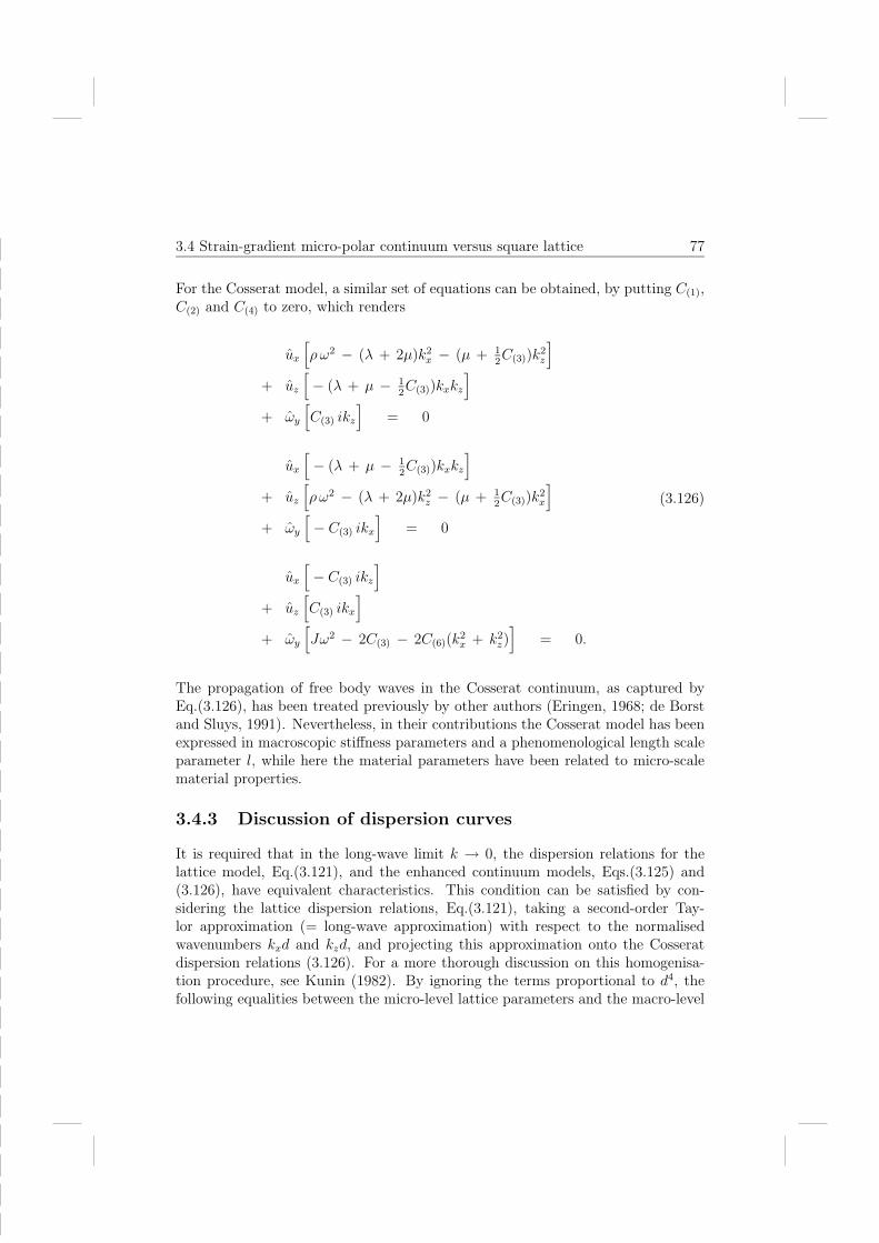
3.4 Strain-gradient micro-polar continuum versus square lattice 77
For the Cosserat model, a similar set of equations can be obtained, by putting C(1),C(2) and C(4) to zero, which renders
ux
[ρω2 − (λ + 2µ)k2
x − (µ + 12C(3))k
2z
]+ uz
[− (λ + µ − 1
2C(3))kxkz
]+ ωy
[C(3) ikz
]= 0
ux
[− (λ + µ − 1
2C(3))kxkz
]+ uz
[ρω2 − (λ + 2µ)k2
z − (µ + 12C(3))k
2x
]+ ωy
[− C(3) ikx
]= 0
ux
[− C(3) ikz
]+ uz
[C(3) ikx
]+ ωy
[Jω2 − 2C(3) − 2C(6)(k
2x + k2
z)]
= 0.
(3.126)
The propagation of free body waves in the Cosserat continuum, as captured byEq.(3.126), has been treated previously by other authors (Eringen, 1968; de Borstand Sluys, 1991). Nevertheless, in their contributions the Cosserat model has beenexpressed in macroscopic stiffness parameters and a phenomenological length scaleparameter l, while here the material parameters have been related to micro-scalematerial properties.
3.4.3 Discussion of dispersion curves
It is required that in the long-wave limit k → 0, the dispersion relations for thelattice model, Eq.(3.121), and the enhanced continuum models, Eqs.(3.125) and(3.126), have equivalent characteristics. This condition can be satisfied by con-sidering the lattice dispersion relations, Eq.(3.121), taking a second-order Tay-lor approximation (= long-wave approximation) with respect to the normalisedwavenumbers kxd and kzd, and projecting this approximation onto the Cosseratdispersion relations (3.126). For a more thorough discussion on this homogenisa-tion procedure, see Kunin (1982). By ignoring the terms proportional to d4, thefollowing equalities between the micro-level lattice parameters and the macro-level

78 Chapter 3. Enhanced continua and discrete lattices to model granular media
continuum parameters are found
M = ρ d3
I = Jd3
Knaxi + Kndia
d= λ + 2µ
2Kndia
d= λ + µ − 1
2C(3)
Kndia + Ksaxi
d= µ + 1
2C(3)
Ksaxi
d= C(3)
Gaxi
2d= C(6)
Ksdia = 0
Gdia = 0.
(3.127)
Clearly, the conditions (3.127-h) and (3.127-i) engender that for the shear and therotational spring contributions only the axial part remains active. The expressionfor µ in terms of the discrete springs can now be found by substituting (3.127-f)into (3.127-e). Then, λ follows from combining (3.127-c) with (3.127-e), as well asfrom combining (3.127-d) with (3.127-e),
µ =2Kndia + Ksaxi
2d
λ(1) =Knaxi − Kndia − Ksaxi
d
λ(2) =Kndia
d.
(3.128)
The two different expressions for λ stem from the anisotropic character of the squarelattice, as represented by the different spring characteristics and the different celldistance in the axial and diagonal direction of the lattice. In order to arrive atan isotropic continuum in the long-wave approximation, it is required that the twoexpressions for λ in (3.128) are equal, which results in the constraint
2Kndia = Knaxi − Ksaxi . (3.129)

3.4 Strain-gradient micro-polar continuum versus square lattice 79
Combining (3.129) with (3.128) now yields for the Lame constants
λ =Knaxi − Ksaxi
2 d
µ =Knaxi
2 d.
(3.130)
Note that the micro-macro relations (3.130-a,-b) and (3.127-f,-g) are different fromthe micro-macro relations presented by Eqs.(3.101-a,-b,-e,-h), respectively. This isdue the fact that a different homogenisation procedure has been used, as well asto the fact that the square lattice reflects a two-dimensional particle configuration,while the second-gradient micro-polar model, Eq.(3.100), has been derived from athree-dimensional particle configuration.The dispersion curves for the square lattice and the enhanced continuum mod-
els can be determined by numerically solving the corresponding set of algebraicequations, Eqs.(3.121), (3.125) and (3.126). A non-trivial solution can be foundif, for a given set of elastic parameters, the determinant ∆(ω, kx, kz) of the spe-cific system of equations is equal to zero. The parameters used for the computa-tion are: λ = 55.5MPa, µ = 83.3MPa, d = 2r = 50mm, C(6) = 69.5 kN ,ρ = 1800 kg/m3 and J = 0.5625 kg/m1. The value for C(6) relates to a micro-levelstiffness ratio Gaxi/Ksaxi = d2, whereas the value for the moment of inertia perunit volume J reflects a medium of equal-sized circular particles, for which themoment of inertia of an individual particle ensues from I = Md2/8.Figure 3.6 depicts the dispersion curves of the compression wave, the shear wave
and the micro-rotation wave. The direction of propagation of the waves corre-sponds to kx, kz = k, 0. Hence, the waves propagate along the x-axis, wherethe wavelength in the z-direction is considered to be infinitely large. For the dis-crete lattice, this causes the first Brillouin zone to be represented by kd ∈ [−π, π].At the end of the first Brillouin zone, all three waves in the discrete lattice attaina frequency maximum, where the group velocity of the waves is zero, cg
x = 0.As mentioned before, these waves may be characterised as standing waves. Forthe second-gradient micro-polar model, the compression wave and the shear wavealso reveal a frequency maximum, though these maxima and the correspondingwavenumbers are smaller than those for the lattice model. The micro-rotationwave in this model does not have a frequency maximum, because the polynomial,Eq.(3.82), describing the contact rotation only contains terms up to and includingthe second order. If this Taylor series had been truncated after the fourth-orderterm, the micro-rotation wave most likely would also have exhibited a frequencymaximum. For the Cosserat model, the Taylor series regarding the contact dis-placement (3.6) and the contact rotation (3.82) are both truncated after the firstorder term, which is the reason why the dispersion curves of this model do not

80 Chapter 3. Enhanced continua and discrete lattices to model granular media
Normalised wavenumber kxd [-]
0 1 2 3 4 5 6 7
Angula
r fr
equency
ω [
rad
/s]
0
5000
10000
15000
20000
25000
30000
35000
Shear
Compr.
Micr. rot.
Cosserat cont.
Sec.-gr. micro-polar cont.
9-cell square lattice
.
Figure 3.6: The ω− kxd dispersion curves for the shear wave (Shear), the compressionwave (Compr.) and the micro-rotation wave (Micr. rot.). - Various models.
exhibit frequency maxima at all.
Up to a wavenumber kx ≈ 2.0/d, which relates to a wavelength Λx ≈ 3.1d,the overall agreement between the second-gradient micro-polar continuum and thelattice is good, in a sense that for the dispersion curves the relative difference infrequency is less than 10%. For the Cosserat model, the accuracy is somewhat less,due to a lesser extent of the Taylor series (3.6) and (3.82).
In Section 3.3, it has been discussed that the constitutive terms C(1) and C(2)
have a destabilising effect on the response of the second-gradient micro-polar model,Eq.(3.100). Although the presence of destabilising terms does not necessarily induceoverall instability, see Section 3.2.2., the second-gradient micro-polar continuumnevertheless becomes unstable for kx > 3.0/d, i.e. when the wavelength of thedeformation pattern becomes smaller than 2.1 times the particle diameter. At thisstage the dispersion curve of the compression wave intersects with the frequencyaxis ω = 0, see Figure 3.6, after which the frequency becomes imaginary andthe response increases exponentially with time. When using the second-gradientmicro-polar model in the analysis of dynamic boundary value problems, wavelengthssmaller than the critical wavelength should be excluded from the response to avoidthe appearance of this physically unrealistic instability.
Instead of using a 9-cell square lattice to reveal the accuracy level of higher-ordercontinua, other lattice configurations could have been chosen as well, such as the7-cell hexagonal lattice described in Suiker et al. (2001c) and Suiker and de Borst

3.5 Discussion 81
(2002). The different topology of the 7-cell hexagonal lattice causes the micro-macro relationships to be different from Eqs.(3.127) and (3.130). Moreover, theanisotropy and inhomogeneity characteristics resulting from the discrete natureof the lattice are different, although this becomes manifest only for very shortdeformation patterns, i.e. when the wavelength is less than 6 times the particlediameter d (Suiker et al., 2001c).
3.5 Discussion
The derivation of continuum formulations for isotropic granular materials consistingof equal-sized spherical particles has been discussed. By employing a homogeni-sation method known as the ’micro-structural approach’, several kinematically-en-hanced continuum models have been derived. The constitutive coefficients in theseenhanced continua have been expressed in terms of micro-structural properties,such as particle radius, contact stiffness and package density. The accuracy levelat which the discrete structure is simulated by the continuum models depends onthe truncation level of the Taylor series used for describing the particle kinematics.This has been illustrated by comparing the dispersion curves of continuum modelswith those of two discrete lattices, which are the one-dimensional Born-Karmanlattice and the two-dimensional 9-cell square lattice.
As exemplified, including only the effect of particle displacement leads to a strain-gradient model, while adding the effect of particle rotation leads to a strain-gradientmicro-polar model. By analysing the dispersion curves for body wave propagation,it has been shown that enhanced continua and discrete lattices may retain waveswith frequencies lying above a specific threshold frequency. This filtering effect isthe result of including the particle size into the model formulation. The maximumfrequency transmitted thereby relates to a minimum transmittable wavelength,which for a discrete lattice equals two times the particle diameter.
The stability of the continuum models has also been examined. It has been shownthat some enhanced continuum models may reveal a physically spurious instabilitywhen the wavelength of the imposed deformation pattern becomes smaller than aspecific critical wavelength. Nonetheless, this occurs at deformation levels wherethe Taylor approximation reflecting the discrete particle kinematics has already lostits accuracy. The critical wavelength at which the instability emerges can be foundeither from examination of the dispersion relations for body wave propagation, orfrom examination of the second-order work. Because of the physically irrationalcharacter of the instability, the use of these models in dynamic boundary valueproblems requires the analyst to exclude deformation components from the responsewith a wavelength smaller than the critical wavelength. Only then, a stable response

82 Chapter 3. Enhanced continua and discrete lattices to model granular media
can be computed. Discrete lattices do not suffer from such a deficiency, since thesemodels describe the particle kinematics in an ’exact manner’. In fact, for discretemodels wavelengths smaller than two times the particle diameter will be naturallyexcluded from the solution to a boundary value problem, as they can not be uniquelyregistered by the particles.

Chapter 4
Dynamic response of a discretegranular layer
In railway systems various structural inhomogeneities can be identified, which arethe discrete ballast particles, the sleeper supports, the irregularities at the railsurface and train wheel surface, differential settlements and stiffness transitions.These inhomogeneities amplify the track response, where the magnitude of theamplification is dependent on a number of aspects, such as the velocity at whicha train axle passes the inhomogeneity, the abruptness of the inhomogeneity, theperiodicity of the inhomogeneity and the train vehicle characteristics. This chapterfocuses on the response characteristics that are due to the discrete nature of theballast particles and the sleeper support. The deformation patterns mostly affectedby these inhomogeneities are the deformation patterns containing wavelengths ofa magnitude similar to the characteristic length of the inhomogeneity, which isrepresented here by the ballast particle size and the sleeper distance, respectively.Such small wavelengths particularly will contribute to the track response whenthe ballast layer is supported by a stiff substratum, i.e. a concrete foundation, aconcrete bridge or a rock formation. Actually, train-induced waves may then reflectone or more times at the stiff ballast-substratum interface, causing the ballastlayer to behave as a wave guide. Accordingly, both long waves with relatively lowfrequencies and short waves with relatively high frequencies are to a certain extentconducted by the layer, see Section 2.4.2. This does not happen when the ballastlayer is supported by a softer substratum, since the relatively short waves then aredirectly dissipated by the substratum, see Section 2.4.1.
In Chapter 3 it was suggested that the discrete nature of a ballast material canbe modelled by employing a discrete lattice model, or a kinematically-enhancedcontinuum model. It is recalled that the approximative character of the kinematicformulation in an enhanced continuum formulation causes this model to lose its

84 Chapter 4. Dynamic response of a discrete granular layer
accuracy in the range of short wavelengths. The loss of accuracy may eventuallybe accompanied by a loss of uniqueness and the emergence of a physically spu-rious instability. Notwithstanding, enhanced continuum models can be correctlyapplied for the analysis of wave propagation phenomena in railway tracks by leav-ing out the response components corresponding to a spurious unstable behaviour,see Suiker et al. (1999a, 1999b). However, since the inhomogeneous nature ofballast is represented more accurately by a lattice model, in this chapter a latticemodel is employed for analysing the dynamic behaviour of a ballast layer. Hereto,a ballast layer modelled by multiple 9-cell square lattices is subjected to a moving,harmonically vibrating load. The moving load is thought to represent an instanta-neous train axle passage, whereas the load frequency represents the sleeper distanceeffect. Trivially, the moving, harmonically vibrating load reduces to a moving loadwith a constant amplitude when the load frequency is prescribed to be equal tozero. The constant load models the dead weight of the train transferred by a trainaxle.
Prior to the analysis of the above-mentioned boundary value problem, the prop-agation of free body waves through the discrete layer is investigated. By combiningthe characteristics of the body waves in an infinite medium with the boundary con-ditions of an undisturbed layer, the dispersion branches that represent the eigenmodes of the discrete layer are derived. It is shown that for a very small particleradius the dispersion branches for a discrete layer approximate those for a continu-ous layer. Furthermore, the typical influence of the particle diameter and the layerthickness on the dynamic characteristics of the layer is illustrated by means of aparametric study.
Subsequently, the steady-state problem regarding the moving load is formulated.The solution procedure is elaborated, and a parametric study is performed to revealhow the layer response is influenced by the particle size, the material viscosity, theload velocity, and the load frequency. Apart from considering the steady-statedisplacement pattern, the frequencies and wavelengths of the waves perturbed bythe moving load are scrutinised by means of a kinematic analysis. It is demonstratedthat for a discrete particle assembly the kinematic characteristics of the movingload are represented by an infinite number of kinematic invariants. The kinematicrepresentation thus considerably differs from that of a load moving on a continuousstructure, in which only one kinematic invariant appears, see Chapter 2.
Finally, the maximum amplitude of the steady state response is computed for arange of load velocities. This is done for both the constant load and the harmonicload. It is exemplified that a larger particle diameter increases the number ofcritical velocities that characterise the resonance of layer vibrations. Because itis of interest to elucidate the genuine differences with a continuous layer model,throughout the analysis the results of the discrete model will be compared to those

4.1 Governing equations for a square lattice 85
of a corresponding continuum model.
It is emphasised that one of the focal points in the present chapter is to revealhow the typically discrete nature of a ballast layer may qualitatively influence itsdynamic response. Apart from related work by the author and co-workers (Suikeret al., 2000, 2001d, 2001e), as yet not much research effort has been invested inthis direction. This may be due to the complexities encountered in the analysis ofwave propagation through discrete models, as well as the large computation timesgenerally associated with discrete modelling.
For limiting the complexity of the analysis, some essential assumptions havebeen made. Firstly, the ballast particles in the layer are assumed to be circularand equal-sized. It is obvious that this is a rather simplified representation of anin-situ ballast layer with arbitrary-shaped particles of various sizes. Secondly, thenon-linear contact behaviour of the ballast particles is approximated by a linearcontact law. Accordingly, energy consumption by reversible frictional sliding ofballast particles, as generated during passage of an instantaneous train axle, istaken into account by means of linear viscous dampers, and pressure-dependentelastic and plastic effects at the particle contacts are left out of consideration.Naturally, a linear contact law brings in limitations to the accuracy of the layermodel, in particular when strong inhomogeneities are generated as a result of large,local pressure differences. On the other hand, in combination with the assumptionof equal-sized particles, a linear contact law provides the discrete model with aconvenient spatial repetitiveness, which avoids the use of a time-consuming discreteelement simulation where the response of all individual particles in the layer needs tobe computed. Thirdly, the discrete character of the ballast particles is simulated bya lattice with pre-defined contacts. Hence, the effect of particle redistributions andre-orienting contact interactions is not taken into account. However, it is expectedthat this does not induce major restrictions, since during the instantaneous passageof a train axle the deformations in the ballast remain relatively small, and theduration of the dynamic loading is relatively short. Especially for a ballast layerthat has been consolidated as a result of a large number of previous train passages,this effect is probably of minor importance.
4.1 Governing equations for a square lattice
Figure 4.1 depicts a rigidly supported layer of equal-sized, circular particles withdiameter d. This configuration is thought to model a ballast layer supported bya very stiff substratum, such as a concrete railway foundation, a concrete railwaybridge or a natural rock formation. Since the substratum behaviour is approxi-mated by an infinitely stiff support, the model is realistic only for waves with a

86 Chapter 4. Dynamic response of a discrete granular layer
wavelength smaller than the layer thickness. The internal layer geometry and themicro-structural particle interactions are simulated by a 9-cell square lattice, wherethe individual cells are connected through elastic longitudinal springs and shearsprings, see Figure 4.2. Here, the cell distance represents the particle diameter.Rotational motions will not be taken into account, as the study in Section 3.4 hasdemonstrated that harmonic particle rotations correspond to very high frequencies,which are expected to be damped for a common ballast material. The angular fre-quency range that will be considered in the analyses equals ω ∈ [0, 10000 rad/s].This range approximately corresponds to a frequency band [0, 1500Hz], which isreckoned to be significant for the vibrations of concrete sleepers in ballasted tracks(Knothe and Grassie, 1993; Grassie, 1995; Nordborg, 1998). Because during aninstantaneous train axle passage concrete sleepers hardly dissipate vibrations, thisfrequency band is supposed to be transmitted almost completely to the ballastunderneath.
Fz
x
Ωexp(i t) δ x(x - v t)
vd
H
0X
Z
Figure 4.1: Moving, harmonically vibrating load on a layer of discrete circular particleswith diameter d.

4.1 Governing equations for a square lattice 87
The equations of motion for the inner cell of the lattice depicted in Figure 4.2 canbe retrieved from those of the more extended square lattice in Section 3.4.1, seeEq.(3.119), by neglecting the rotational contributions. This leads to
Mu(m,n)x =
12Knaxi
[− 4u(m,n)
x + 2u(m+1,n)x + 2u(m−1,n)
x
]
+12Kndia
[− 4u(m,n)
x + u(m+1,n+1)x + u(m+1,n−1)
x + u(m−1,n+1)x + u(m−1,n−1)
x
+ u(m+1,n+1)z + u
(m−1,n−1)z − u
(m+1,n−1)z − u
(m−1,n+1)z
]
+12Ksaxi
[− 4u(m,n)
x + 2u(m,n+1)x + 2u(m,n−1)
x
]
+12Ksdia
[− 4u(m,n)
x + u(m+1,n+1)x + u(m+1,n−1)
x + u(m−1,n−1)x + u(m−1,n+1)
x
+ u(m+1,n−1)z + u
(m−1,n+1)z − u
(m−1,n−1)z − u
(m+1,n+1)z
]
Mu(m,n)z =
12Knaxi
[− 4u(m,n)
z + 2u(m,n+1)z + 2u(m,n−1)
z
]
+12Kndia
[− 4u(m,n)
z + u(m+1,n+1)z + u(m+1,n−1)
z + u(m−1,n−1)z + u(m−1,n+1)
z
+ u(m+1,n+1)x + u
(m−1,n−1)x − u
(m+1,n−1)x − u
(m−1,n+1)x
]
+12Ksaxi
[−4u(m,n)
z + 2u(m+1,n)z + 2u(m−1,n)
z
]
+12Ksdia
[− 4u(m,n)
z + u(m+1,n+1)z + u(m+1,n−1)
z + u(m−1,n+1)z + u(m−1,n−1)
z
+ u(m+1,n−1)x + u
(m−1,n+1)x − u
(m+1,n+1)x − u
(m−1,n−1)x
].
(4.1)In addition to the introduction of inner cells to construct the interior of the layer,boundary cells are introduced to construct the free surface of the layer. Figure4.3 shows the topology of the boundary cell and its neighbours, which has beendeduced from the topology of the inner cell and its neighbours by omitting thethree neighbouring cells on top of the inner cell.

88 Chapter 4. Dynamic response of a discrete granular layer
Hence, the equations of motion for the boundary cell are derived from Eq.(4.1) as
Mu(m,0)x =
12Knaxi
[− 4u(m,0)
x + 2u(m+1,0)x + 2u(m−1,0)
x
]
+12Kndia
[− 2u(m,0)
x + u(m+1,1)x + u(m−1,1)
x + u(m+1,1)z − u(m−1,1)
z
]
+12Ksaxi
[− 2u(m,0)
x + 2u(m,1)x
]
+12Ksdia
[− 2u(m,0)
x + u(m+1,1)x + u(m−1,1)
x + u(m−1,1)z − u(m+1,1)
z
]
Mu(m,0)z =
12Knaxi
[− 2u(m,0)
z + 2u(m,1)z
]
+12Kndia
[− 2u(m,0)
z + u(m+1,1)z + u(m−1,1)
z + u(m+1,1)x − u(m−1,1)
x
]
+12Ksaxi
[− 4u(m,0)
z + 2u(m+1,0)z + 2u(m−1,0)
z
]
+12Ksdia
[− 2u(m,0)
z + u(m+1,1)z + u(m−1,1)
z + u(m−1,1)x − u(m+1,1)
x
].
(4.2)
+
(m+1,n+1)
(m+1,n)
(m,n-1) (m+1,n-1)
u
Ks
Inner cell of square lattice
z
axi
dia
axi
dia
xu
Ks
Kn
Kn
(m-1,n-1)
(m-1,n)
(m,n+1)(m-1,n+1)
(4)
(5)(6)
(7)
(1)
(8)
(2)
(3)
dd
dd
Figure 4.2 : Connectivity of an inner cell (m,n) in a square lattice.

4.1 Governing equations for a square lattice 89
4.1.1 Lattice model versus continuum model
In order to have a consistent relation between the macro-scale material behaviourand the micro-scale material behaviour, in the long-wave limit the dynamic char-acteristics of the discrete lattice need to be equal to those of an elastic continuum(Born and Huang, 1954; Maradudin et al., 1971; Kunin, 1983; Suiker et al., 2001c).In Chapter 3, this requirement was met by mapping the long-wave approxima-tion of the lattice dispersion relations onto the continuum dispersion relations. Analternative procedure to follow is to project the long-wave approximation of thelattice wave equations onto the continuum wave equations. To this end, the dis-crete degrees of freedom of the cell (m,n) in Eq.(4.1) are replaced by correspondingcontinuous field variables
u(m,n)x (t), u(m,n)
z (t) → ux(x, z, t), uz(x, z, t)∣∣∣x=md, z=nd
, (4.3)
in which the lower bar denotes the continuous character of the degree of freedom.Subsequently, in Eq.(4.1) the degrees of freedom of the neighbouring cells of cell(m,n), located at points (x = (m+ p)d, z = (n+ q)d ), must be replaced by the
(m,1)
Ks
Ks
+dia
ux
zu
Boundary cell of square lattice
diaKn
(m-1,0) (m+1,0)
(m-1,1) (m+1,1)
Kn axiaxi
d
d d
Figure 4.3 : Connectivity of a boundary cell (m, 0) in a square lattice.

90 Chapter 4. Dynamic response of a discrete granular layer
second-order Taylor approximation of the corresponding continuous field variables
u(m+p,n+q)x , u
(m+p,n+q)z ≈
ux, uz + pdux,x, uz,x + qdux,z, uz,z
+ 12p
2d2ux,xx, uz,xx + 12q
2d2ux,zz, uz,zz + pqd2ux,xz, uz,xz∣∣∣∣
x=md, z=nd
.
(4.4)In this way, the following equations of motion are obtained
Mux,tt = (Knaxi + Kndia + Ksdia) d2ux,xx + 2 (Kndia + Ksdia) d
2uz,xz
+ (Ksaxi + Kndia + Ksdia) d2ux,zz
Muz,tt = (Knaxi + Kndia + Ksdia) d2uz,zz + 2 (Kndia + Ksdia) d
2ux,zx
+ (Ksaxi + Kndia + Ksdia) d2uz,xx .
(4.5)
Projection of Eq.(4.5) onto the equations of motion for a classic elastic continuum,
ρux,tt = (λ + 2µ)ux,xx + (λ + µ)uz,xz + µux,zz
ρuz,tt = (λ + 2µ)uz,zz + (λ + µ )ux,zx + µuz,xx ,(4.6)
yields the micro-macro relationships,
M = ρ d3
Knaxi + Kndia
d= λ + 2µ
2Kndia
d= λ + µ
Kndia + Ksaxi
d= µ
Ksdia = 0.
(4.7)
To match an anisotropic lattice model with an isotropic continuum model, the shearstiffness in the diagonal direction is set equal to zero, see Eq.(4.7-e). For the samereason, combining Eq.(4.7-d) successively with (4.7-c) and Eq.(4.7-b) provides twodifferent relations for the Lame constant λ,
λ(1) =Knaxi − Kndia − 2Ksaxi
d
λ(2) =Kndia − Ksaxi
d.
(4.8)
Requiring Eqs.(4.8-a) and (4.8-b) to be equivalent results in the constraint
2Kndia = Knaxi − Ksaxi , (4.9)

4.1 Governing equations for a square lattice 91
which is similar to the constraint found for the more extended 9-cell square latticein Chapter 3, see Eq.(3.129). Now, inserting Eq.(4.9) into Eqs.(4.8) and (4.7-d)gives for the Lame constants λ en µ
λ =Knaxi − 3Ksaxi
2 d
µ =Knaxi + Ksaxi
2 d.
(4.10)
Note that Eq.(4.10) differs from the micro-macro expression (3.130) for a micro-polar medium, which is due to the appearance of additional (rotational) stiff-nesses in the constitutive expressions for a micro-polar medium. When substitutingEqs.(4.9) and (4.7-e) into Eq.(4.1), the equations of motion for the inner cell (m,n)become
Mu(m,n)x = Knaxi
[− 3u
(m,n)x + u
(m+1,n)x + u
(m−1,n)x + 1
4
(u
(m+1,n+1)x + u
(m−1,n+1)x
+ u(m−1,n−1)x + u
(m+1,n−1)x
)+ 1
4
(u
(m+1,n+1)z + u
(m−1,n−1)z
− u(m+1,n−1)z − u
(m−1,n+1)z
) ]+ Ksaxi
[− u
(m,n)x + u
(m,n+1)x + u
(m,n−1)x
− 14
(u
(m+1,n+1)x + u
(m−1,n+1)x + u
(m−1,n−1)x + u
(m+1,n−1)x
)− 1
4
(u
(m+1,n+1)z + u
(m−1,n−1)z − u
(m+1,n−1)z − u
(m−1,n+1)z
) ]Mu
(m,n)z = Knaxi
[− 3u
(m,n)z + u
(m,n+1)z + u
(m,n−1)z + 1
4
(u
(m+1,n+1)z + u
(m+1,n−1)z
+ u(m−1,n−1)z + u
(m−1,n+1)z
)+ 1
4
(u
(m+1,n+1)x + u
(m−1,n−1)x
− u(m+1,n−1)x − u
(m−1,n+1)x
) ]+ Ksaxi
[− u
(m,n)z + u
(m+1,n)z + u
(m−1,n)z
− 14
(u
(m+1,n+1)z + u
(m+1,n−1)z + u
(m−1,n−1)z + u
(m−1,n+1)z
)− 1
4
(u
(m+1,n+1)x + u
(m−1,n−1)x − u
(m+1,n−1)x − u
(m−1,n+1)x
) ].
(4.11)

92 Chapter 4. Dynamic response of a discrete granular layer
Additionally, substituting these constraints into the equation of motion for theboundary cell (m, 0), Eq.(4.2), results in
Mu(m,0)x =
1
2Knaxi
[− 5u(m,0)
x + 2u(m+1,0)x + 2u(m−1,0)
x + 12u(m+1,1)
x + 12u(m−1,1)
x
+ 12u
(m+1,1)z − 1
2u
(m−1,1)z
]+
1
2Ksaxi
[− u(m,0)
x + 2u(m,1)x − 1
2u(m+1,1)
x
− 12u
(m−1,1)x − 1
2u
(m+1,1)z + 1
2u
(m−1,1)z
]
Mu(m,0)z =
1
2Knaxi
[− 3u(m,0)
z + 2u(m,1)z + 1
2u(m+1,1)
z + 12u(m−1,1)
z + 12u(m+1,1)
x
− 12u
(m−1,1)x
]+
1
2Ksaxi
[− 3u(m,0)
z + 2u(m+1,0)z + 2u(m−1,0)
z − 12u(m+1,1)
z
− 12u
(m−1,1)z − 1
2u
(m+1,1)x + 1
2u
(m−1,1)x
].
(4.12)
4.2 Dispersion curves of the body waves
Now that the equations of motion for the inner cell have been determined, thepropagation of body waves through an infinite lattice can be analysed. To this end,a solution of expression (4.11) will be sought in the form of plane harmonic waves
u(m,n)x = ux exp
(i(ωt − mkxd − nkzd)
)u
(m,n)z = uz exp
(i(ωt − mkxd − nkzd)
).
(4.13)
Substitution of Eq.(4.13) into Eq.(4.11) renders
ux
[Mω2 + Knaxi
(2 cos(kxd) + cos(kxd) cos(kzd) − 3
)+ Ksaxi
(2 cos(kzd) − cos(kxd) cos(kzd) − 1
)]+ uz
[(Knaxi − Ksaxi)
(− sin(kxd) sin(kzd)
)]= 0
ux
[(Knaxi − Ksaxi)
(−sin(kxd) sin(kzd)
)]+ uz
[Mω2 + Knaxi
(2 cos(kzd) + cos(kxd) cos(kzd) − 3
)+ Ksaxi
(2 cos(kxd) − cos(kxd) cos(kzd) − 1
)]= 0.
(4.14)

4.2 Dispersion curves of the body waves 93
The system of equations (4.14) has a non-trivial solution if, for a given set of elasticparameters, its determinant ∆(ω, kx, kz) is equal to zero, i.e.[
Mω2 + Knaxi
(cos(kxd) + cos(kzd) + 2 cos(kxd) cos(kzd) − 4
)+ Ksaxi
(cos(kxd) + cos(kzd) − 2 cos(kxd) cos(kzd)
)]×[Mω2 + (Knaxi + Ksaxi)
(cos(kxd) + cos(kzd) − 2
)]= 0.
(4.15)
In Eq.(4.15), the first (second) expression between square brackets characterises thepropagation of the compression wave (shear wave). The character of the dispersionrelations (4.15) depends on the direction of the body wave propagation, as the parti-cle diameter d causes the lattice to behave increasingly anisotropic for a decreasingwavelength (see for instance, Brillouin, 1946; Kunin, 1983; Suiker et al., 2001c).When considering the body waves to be propagating along a prescribed direction,e.g. the x-axis, an infinite number of dispersion curves can be constructed, whereeach dispersion curve is characterised by its wavenumber kz in the z-direction. Forboth the compression wave and the shear wave, the domain of dispersion curves isenclosed by a lower frequency branch and an upper frequency branch. The lower fre-quency branch is determined by the minimum value for the normalised wavenumberin z-direction; kzd = 0, whereas the upper frequency branch ensues upon adopt-ing a maximum value for the normalised wavenumber in z-direction; kzd = π (orkzd = −π). The backgrounds of the maximum normalised wavenumber will betreated in more detail later in this section.In Figure 4.4 the dispersion curves corresponding to the propagation of the com-
pression wave and the shear wave in an infinite medium are depicted. The dispersioncurves have been computed by using a Young’s modulus E = 200MPa, a Poisson’sratio ν = 0.20 (corresponding to Lame constants λ = 55.5MPa, µ = 83.3MPa)and a density ρ = 1800 kg/m3. These parameters constitute a moderately consoli-dated ballast material. The lattice cell distance d, which equals the diameter of theballast particles, has been chosen as d = 100mm This is the largest particle sizethat can be found in a broadly-graded ballast. The diameter d and the Lame con-stants λ and µ provide the particle contact stiffnesses Knaxi and Ksaxi by inversionof Eq.(4.10).Figure 4.4 depicts the lower frequency branch and the upper frequency branch of
the shear wave and the compression wave. The considered wavenumber domain hasbeen limited to the first Brillouin zone, as for discrete systems higher wavenumbersare irrelevant, see Section 3.2.3. The material frame indifference can be observedfrom the equal frequency values for the cases [kxd = 0, kzd = π] (= frequencyvalues for upper branches at kxd = 0) and [kxd = π, kzd = 0] (= frequency values

94 Chapter 4. Dynamic response of a discrete granular layer
for lower branches at kxd = π). At the end of the first Brillouin zone the slope ofthe dispersion curves is horizontal, representing a standing wave. Furthermore, inthe long wave limit kxd → 0, the tangential slope of the lower branches correspondsto the body wave velocities in a classic linear elastic medium, i.e.
Compression wave : ckx→0x = cP =
√(3Knaxi − Ksaxi) d
2
2M=
√λ + 2µ
ρ
Shear wave : ckx→0x = cS =
√(Knaxi + Ksaxi)d
2
2M=
õ
ρ.
(4.16)The characteristics of the body waves in an infinite medium will be employed laterin the analysis of the waves propagating through the layer.
Normalised wavenumber kxd [-]
0.0 0.5 1.0 1.5 2.0 2.5 3.0 3.5
Angula
r fr
equency
ω
[rad
/s]
0
2000
4000
6000
8000
10000
Lower branches
Upper branches
end of 1st Brillouin zone
Compression waveShear wave
cP
cS
Figure 4.4: Body wave dispersion curves for the 9-cell square lattice in Figure 4.2.Upper frequency branches (kzd = 0) and lower frequency branches (kzd = π).

4.2 Dispersion curves of the body waves 95
Hence, Eq.(4.15) is solved for the wavenumber kz, yielding the following expressions
k(1),(2)z = ±1
darccos
Mω2 + Knaxi
(cos(kxd) − 4
)+ Ksaxi cos(kxd)
−Knaxi
(2 cos(kxd) + 1
)+ Ksaxi
(2 cos(kxd) − 1
)
k(3),(4)z = ±1
darccos
−Mω2 − Knaxi
(cos(kxd) − 2
)− Ksaxi
(cos(kxd) − 2
)Knaxi + Ksaxi
.
(4.17)In agreement with the four solutions k
(j)z , the amplitude vectors of the harmonic
solutions (4.13) consist of four components: ux = [u(1)x , u
(2)x , u
(3)x , u
(4)x ]T and uz =
[u(1)z , u
(2)z , u
(3)z , u
(4)z ]T . The eigen vector D, which contains the amplitude ratios of
the body waves u(j)z /u
(j)x , ensues from either Eq.(4.14-a) or Eq.(4.14-b). The former
relation provides the following vector components
D(j) =u
(j)z
u(j)x
=[Mω2 + Knaxi
(2 cos(kxd) + cos(kxd) cos(k
(j)z d) − 3
)+ Ksaxi
(2 cos(k
(j)z d) − cos(kxd) cos(k
(j)z d) − 1
)]×[ (
Knaxi − Ksaxi
)sin(kxd) sin(k
(j)z d)
]−1
with j ∈ 1, 2, 3, 4.(4.18)
Combining Eqs.(4.13), (4.17) and (4.18), the displacements corresponding to har-monic body wave propagation may now be generally formulated as
u(m,n)x =
(u
(1)x exp(−ink
(1)z d) + u
(2)x exp(−ink
(2)z d) + u
(3)x exp(−ink
(3)z d)
+ u(4)x exp(−ink
(4)z d)
)exp(i(ωt − mkxd)
)
u(m,n)z =
(u
(1)x D(1)exp(−ink
(1)z d) + u
(2)x D(2)exp(−ink
(2)z d) + u
(3)x D(3)exp(−ink
(3)z d)
+ u(4)x D(4)exp(−ink
(4)z d)
)exp(i(ωt − mkxd)
).
(4.19)

96 Chapter 4. Dynamic response of a discrete granular layer
4.3 Dispersion branches of the layer modes
The solutions obtained in the previous section concerned the body wave propagationthrough an infinite medium. When body waves meet the top or the bottom of thelayer, their propagation characteristics are modified into those of the so-called freewaves in the layer. Typically, the steady state propagation of these free wavesis characterised by the dispersion branches that represent the eigen modes of thelayer. For the configuration depicted in Figure 4.1, the eigen modes can be derivedby requiring the boundary cells at the top of the layer z = 0 to be loading-free.Hence, these boundary conditions are equal to the equations of motion for the freeboundary cell, i.e. Eq.(4.12),
Mu(m,0)x =
1
2Knaxi
[− 5u(m,0)
x + 2u(m+1,0)x + 2u(m−1,0)
x + 12u(m+1,1)
x + 12u(m−1,1)
x
+ 12u
(m+1,1)z − 1
2u
(m−1,1)z
]+
1
2Ksaxi
[− u(m,0)
x + 2u(m,1)x − 1
2u(m+1,1)
x
− 12u
(m−1,1)x − 1
2u
(m+1,1)z + 1
2u
(m−1,1)z
]
Mu(m,0)z =
1
2Knaxi
[− 3u(m,0)
z + 2u(m,1)z + 1
2u(m+1,1)
z + 12u(m−1,1)
z + 12u(m+1,1)
x
− 12u
(m−1,1)x
]+
1
2Ksaxi
[− 3u(m,0)
z + 2u(m+1,0)z + 2u(m−1,0)
z − 12u(m+1,1)
z
− 12u
(m−1,1)z − 1
2u
(m+1,1)x + 1
2u
(m−1,1)x
].
(4.20)Furthermore, the bottom of the layer is assumed to be rigidly supported, such thatthe displacements at z = nd = H are equal to zero,
u(m,H/d)x = 0
u(m,H/d)z = 0.
(4.21)

4.3 Dispersion branches of the layer modes 97
Substitution of the expressions for body wave propagation (4.19) into the boundaryconditions (4.20) and (4.21) yields the following set of algebraic equations[u
(1)x + u
(2)x + u
(3)x + u
(4)x
] (Mω2 + 1
2Knaxi
(4 cos(kxd) − 5
) − 12Ksaxi
)+[u
(1)x exp(−ik
(1)z d) + u
(2)x exp(−ik
(2)z d) + u
(3)x exp(−ik
(3)z d) + u
(4)x exp(−ik
(4)z d)
]×(
12Knaxi cos(kxd) − 1
2Ksaxi
(cos(kxd) − 2
))+[u
(1)x D(1)exp(−ik
(1)z d) + u
(2)x D(2)exp(−ik
(2)z d) + u
(3)x D(3)exp(−ik
(3)z d)
+ u(4)x D(4)exp(−ik
(4)z d)
] (− 1
2 iKnaxi sin(kxd) + 12 iKsaxi sin(kxd)
)= 0
[u
(1)x D(1) + u
(2)x D(2) + u
(3)x D(3) + u
(4)x D(4)
] (Mω2 − 3
2Knaxi + 12Ksaxi
(4 cos(kxd)− 3
))+[u
(1)x D(1)exp(−ik
(1)z d) + u
(2)x D(2)exp(−ik
(2)z d) + u
(3)x D(3)exp(−ik
(3)z d)
+ u(4)x D(4)exp(−ik
(4)z d)
] (12Knaxi
(cos(kxd) + 2
) − 12Ksaxi cos(kxd)
)+[u
(1)x exp(−ik
(1)z d) + u
(2)x exp(−ik
(2)z d) + u
(3)x exp(−ik
(3)z d) + u
(4)x exp(−ik
(4)z d)
]×(− 1
2 iKnaxi sin(kxd) + 12 iKsaxi sin(kxd)
)= 0
u(1)x exp(−ik
(1)z H) + u
(2)x exp(−ik
(2)z H) + u
(3)x exp(−ik
(3)z H) + u
(4)x exp(−ik
(4)z H) = 0
u(1)x D(1)exp(−ik
(1)z H) + u
(2)x D(2)exp(−ik
(2)z H) + u
(3)x D(3)exp(−ik
(3)z H)
+ u(4)x D(4)exp(−ik
(4)z H) = 0,
(4.22)
in which k(j)z and D(j) are given by the Eqs.(4.17) and (4.18), respectively. The
relations (4.22) can be expressed in a matrix-vector format as
E ux = 0, (4.23)
where E is a 4 × 4 matrix that governs the eigen behaviour of the layer, andux = [u
(1)x , u
(2)x , u
(3)x , u
(4)x ]T is the vector that assembles the wave amplitudes. The
dispersion branches of the eigen modes can be obtained by requiring the determi-nant of the matrix E to be equal to zero, which for a given set of elastic parametersrenders
detE = ∆(ω, kx, H, d) = 0. (4.24)
For a prescribed layer thickness H and particle diameter d, expression (4.24) yieldsa finite number of eigen modes
ω(j) = ω (kx)(j) with j = 1, 2, ..., N, (4.25)

98 Chapter 4. Dynamic response of a discrete granular layer
where the total number of modes N depends on the magnitude of the particle sizeand the layer thickness. This will be exemplified in a qualitative sense later in thischapter.In order to illustrate the specific features of the eigen modes of the discrete layer,
the corresponding dispersion branches (4.25) will be compared to the dispersionbranches for a classic elastic continuous layer. For obvious reasons, the dispersionbranches for the continuous layer can be computed in the same manner as shownabove for the discrete layer. When considering the top of the continuous layeras stress-free, i.e. σzz = 0, σzx = 0, and the bottom as rigidly supported, i.e.ux = 0, uz = 0, similar to Eq.(4.22), a set of four characteristic equations can bederived
u(1)x
(k
(1)z + D
(1)kx
)+ u
(2)x
(k
(2)z + D
(2)kx
)+ u
(3)x
(k
(3)z + D
(3)kx
)+ u
(4)x
(k
(4)z + D
(4)kx
)= 0
−[u
(1)x + u
(2)x + u
(3)x + u
(4)x
]i λ kx −
[u
(1)x D
(1)k
(1)z + u
(2)x D
(2)k
(2)z + u
(3)x D
(3)k
(3)z
+ u(4)x D
(4)k
(4)z
]i (λ + 2µ) = 0
u(1)x exp(−ik
(1)z H) + u
(2)x exp(−ik
(2)z H) + u
(3)x exp(−ik
(3)z H) + u
(4)x exp(−ik
(4)z H) = 0
u(1)x D
(1)exp(−ik
(1)z H) + u
(2)x D
(2)exp(−ik
(2)z H) + u
(3)x D
(3)exp(−ik
(3)z H)
+ u(4)x D
(4)exp(−ik
(4)z H) = 0,
(4.26)in which the vector ux = [u(1)
x , u(2)x , u(3)
x , u(4)x ]T assembles the wave amplitudes, the
lower bar indicating that a continuum is concerned. Further, the four expressionsfor the wavenumber in z-direction k(j)
z are given by
k(1),(2)z = ±
√ρω2 − µ k2
x
µ
k(3),(4)z = ±
√ρω2 − (λ + 2µ) k2
x
λ + 2µ,
(4.27)
whereas the amplitude ratios D(j)
are
D(j)
=u(j)
z
u(j)x
=ρω2 − (λ + 2µ) k2
x − µ (k(j)z )2
(λ + µ) kx k(j)z
with j ∈ 1, 2, 3, 4.(4.28)

4.3 Dispersion branches of the layer modes 99
In correspondence with Eqs.(4.27) and (4.28), the body wave propagation througha continuum is then expressed as
ux =(u(1)
x exp(−ik(1)z z) + u(2)
x exp(−ik(2)z z) + u(3)
x exp(−ik(3)z z)
+ u(4)x exp(−ik(4)
z z))exp(i(ωt − kxx)
)uz =
(u(1)
x D(1)exp(−ik(1)
z z) + u(2)x D
(2)exp(−ik(2)
z z) + u(3)x D
(3)exp(−ik(3)
z z)
+ u(4)x D
(4)exp(−ik(4)
z z))exp(i(ωt − kxx)
).
(4.29)The general form above closely resembles Eq.(4.19) for the discrete model. Dueto the complex character of Eqs.(4.22) and (4.26), the dispersion branches for thediscrete layer and the continuous layer need to be derived numerically. In thefollowing section, this will be done for various parameter sets.
4.3.1 Variation of particle size
The dispersion branches corresponding to the four lowest eigen modes of the dis-crete layer (solid lines) and the continuous layer (dashed lines) have been computedby using the ballast material parameters given in Section 4.2. The particle radiusis initially chosen relatively small, r = 0.5 d = 1mm, whereas the layer thicknessis assumed as H = 300mm. The result has been depicted in Figure 4.5. Thedispersion branches for a continuous layer have been previously discussed by otherinvestigators (see for example, Ewing et al., 1957; Achenbach, 1973; Dietermanand Metrikine, 1997a), though in their contributions, instead of using the actualdisplacements, the potentials presented in Eq.(2.8) were employed. As a result ofthe small particle size, in the considered ω − kx domain the dispersion branchesfor the discrete layer and the continuous layer closely agree. Apparently, for boththe discrete layer and the continuous layer it looks as if the individual dispersionbranches locally intersect. However, because the eigen modes of the layer are cou-pled, the individual dispersion branches may approach each other very closely, butthere is no contact.For the continuous layer the total number of eigen modes is infinite. This is
different for the discrete layer, which distinguishes a finite number of eigen modesas a result of the frequency filtering effect of the particles. The highest eigenmode possible thereby approaches the upper frequency branch of the compressionbody wave. More specifically, in the frequency range where body waves cannotbe transmitted, eigen modes of the layer will also not exist. Although in Figure4.5 only the four lowest eigen modes of the discrete layer have been depicted,in actual fact a very large number of eigen modes exists. This is, because for

100 Chapter 4. Dynamic response of a discrete granular layer
a relatively small particle radius r = 1mm, the bounding behaviour of the upperfrequency body wave branch occurs in the very high frequency range. By increasingthe particle size to r = 50mm, the upper frequency branch for the body wavesconsiderably descends along the frequency axis, causing the total number of modesto reduce to only six. This is shown in Figure 4.6, in which the corresponding layerdispersion branches are plotted together with the body wave dispersion curves. Thecharacteristic limitation of the layer modes by the envelope of the high-frequencybody wave dispersion curves is clearly illustrated. It can also be noticed that at theend of the first Brillouin zone, kxd = π, all dispersion branches show a horizontaltangential slope. The zero group velocity at this stage implies that no wave energyis conducted anymore, which degenerates the modes into standing waves.As for the body wave dispersion curves, the dispersion branches for the eigen
modes of the discrete layer are periodical with respect to the Brillouin zones, i.e.
ω (kx)(j) = ω
(kx +
2π n
d
)(j)
, (4.30)
with j the mode number and n an arbitrary integer, n ∈ Z. However, for reasonsmentioned previously, the eigen modes have no clear physical meaning for wave-lengths smaller than two times the particle diameter. In Figure 4.6 this minimum
Wavenumber kx [m-1
]
0 5 10 15 20 25 30 35
Angula
r fr
equency
ω [
rad
/s]
0
2000
4000
6000
8000
10000
Discrete layer, r =1mm, H=300mm
Continuous layer, H=300mm
Figure 4.5: Dispersion branches for the four lowest eigen modes of the discrete layer(solid lines, r = 1mm, H = 300mm) and the continuous layer (dashed lines, H =300mm).

4.3 Dispersion branches of the layer modes 101
Wavenumber kx [m-1
]
0 5 10 15 20 25 30 35
Angula
r fr
equency
ω [
rad
/s]
0
2000
4000
6000
8000
10000
end of 1st
Brillouin zone
r = 50mmH = 300mm
Layer modes
Body waves
Figure 4.6: Dispersion branches for the eigen modes (solid lines) and the body waves(dashed lines) of the discrete layer (r = 50mm, H = 300mm). The total number ofeigen modes of the discrete layer equals six.
wavelength is reflected by a maximum wavenumber of kmaxx = π/d ≈ 31.4m−1,
which thus borders the first Brillouin zone.
4.3.2 Variation of layer thickness
In order to investigate how the characteristics of the layer modes are influencedby the layer thickness, the layer thickness is increased from 300mm to 600mmwhile the particle radius is kept constant, r = 50mm. Figure 4.7 shows that thetotal number of layer modes then increases from six to twelve. The reason for theincreased number of layer modes is that a thicker layer reduces the frequencies ofthe modes, thereby causing more modes to be captured in the domain bordered bythe envelope of the high-frequency body wave dispersion curves.
The current parametric study has demonstrated that the magnitude of the min-imum transmittable wavelength only depends on the size of the particles. In con-trast, the total number of layer modes is determined by both the particle size andthe layer thickness. For reasons of clarity, the influence of these two length-scaleparameters on the dispersion branches has been considered by means of separategraphs, instead of basing the discussion on a proper normalisation of the resultsthat might lead to a single, dimensionless graphical representation. The latter wayof representation is commonly chosen when analysing the dispersion branches of a

102 Chapter 4. Dynamic response of a discrete granular layer
Wavenumber kx [m-1
]
0 5 10 15 20 25 30 35
Angula
r fr
equency
ω [
rad
/s]
0
2000
4000
6000
8000
10000
end of 1st
Brillouin zone
r = 50mmH = 600mm
Layer modes
Body waves
Figure 4.7: Dispersion branches for the eigen modes (solid lines) and the body waves(dashed lines) of the discrete layer (r = 50mm, H = 600mm). The total number ofeigen modes of the discrete layer equals twelve.
continuous layer with only one length-scale parameter, i.e. the layer thickness (seefor instance, Ewing et al., 1957).
4.4 Formulation and solution procedure of the
boundary value problem
In the previous section, the characteristics of the free waves propagating throughthe discrete layer have been determined. In order to examine how these waves areperturbed by a moving, harmonically vibrating load, the boundary value problemtreated in the previous section needs to be extended with incorporation of themoving load signature. The current section treats the solution procedure of thisboundary value problem, resulting in expressions for the steady state displacementsin the layer. Also, the expressions required for the performance of a kinematicanalysis are derived.
4.4.1 Derivation of steady state displacements
To determine the steady state displacements u(m,n)x , u
(m,n)z generated in the layer
under a moving, harmonically vibrating load, four conditions at the layer bound-

4.4 Formulation and solution procedure of the boundary value problem 103
aries have to be met. The two boundary conditions at the top of the layer (z = 0)follow from the dynamic balance of forces acting on the free boundary cell. Byusing the equations of motion for the boundary cell, Eq.(4.12), and adding theformulation for the moving harmonically vibrating load, these boundary conditionsbecome
Mu(m,0)x =
1
2Knaxi
[− 5u(m,0)
x + 2u(m+1,0)x + 2u(m−1,0)
x + 12u(m+1,1)
x + 12u(m−1,1)
x
+ 12u
(m+1,1)z − 1
2u
(m−1,1)z
]+1
2Ksaxi
[− u(m,0)
x + 2u(m,1)x − 1
2u(m+1,1)
x
− 12u
(m−1,1)x − 1
2u
(m+1,1)z + 1
2u
(m−1,1)z
]
Mu(m,0)z =
1
2Knaxi
[− 3u(m,0)
z + 2u(m,1)z + 1
2u(m+1,1)
z + 12u(m−1,1)
z + 12u(m+1,1)
x
− 12u
(m−1,1)x
]+1
2Ksaxi
[− 3u(m,0)
z + 2u(m+1,0)z + 2u(m−1,0)
z − 12u(m+1,1)
z
− 12u
(m−1,1)z − 1
2u
(m+1,1)x + 1
2u
(m−1,1)x
]+ dFz exp(iΩt) δ(md − vxt) .
(4.31)In Eq.(4.31-b), the load magnitude Fz has been multiplied by the horizontal celldistance d, which equals the particle diameter. This multiplication provides theloading term with the same dimension as the remaining terms in this expression.Furthermore, Knaxi and Ksaxi are the operators
Knaxi = Knaxi + Cnaxid
d t
Ksaxi = Ksaxi + Csaxid
d t,
(4.32)
in which Cnaxi is the discrete longitudinal viscosity and Csaxi is the discrete shearviscosity. The viscosity can be thought to represent the dissipation due to reversiblefrictional sliding of particles during a load cycle, or train axle passage (Verruijt,1999), see Figure 4.8. Indeed, by neglecting the viscosities in Eq.(4.32), the op-
Figure 4.8 : Reversible frictional sliding of particles during a load cycle.

104 Chapter 4. Dynamic response of a discrete granular layer
erators reduce to the discrete longitudinal stiffness Knaxi and the discrete shearstiffness Ksaxi, respectively. In the same way as the discrete stiffnesses can be re-lated to the Lame constants, see Eq.(4.10), the discrete viscosities can be relatedto the representative macroscopic viscosity parameters λ∗ and µ∗, as used in thewell-known Voigt model (Kolsky, 1963),
λ∗ =Cnaxi − 3Csaxi
2 d
µ∗ =Cnaxi + Csaxi
2 d.
(4.33)
In addition to the two boundary conditions (4.31) at the top of the layer, twoboundary conditions at the bottom of the layer must be formulated. The supportat the bottom of the layer (z = nd = H) is supposed to be rigid, in correspondencewith the boundary conditions presented in Eq.(4.21). To satisfy the boundaryconditions (4.31) and (4.21), the following Fourier transforms with respect to timet are employed
u(m,n)x (ω) =
∫ ∞
−∞u(m,n)
x (t) exp(−iωt) dt
u(m,n)z (ω) =
∫ ∞
−∞u(m,n)
z (t) exp(−iωt) dt
d Fz
vx
exp
(imd
vx
(Ω − ω)
)=
∫ ∞
−∞dFz exp(i Ωt) δ(md − vxt) exp(−i ωt) dt,
(4.34)
with u(m,n)x , u
(m,n)z the Fourier displacements, where the superimposed tilde indi-
cates a single transformation.

4.4 Formulation and solution procedure of the boundary value problem 105
Applying the transformations (4.34) to Eqs.(4.31) and (4.21) leads to
Mω2 u(m,0)x +
1
2
(Knaxi + i ωCnaxi
) [− 5u(m,0)
x + 2u(m+1,0)x + 2u(m−1,0)
x
+ 12u
(m+1,1)x + 1
2u
(m−1,1)x + 1
2u
(m+1,1)z − 1
2u
(m−1,1)z
]+
1
2
(Ksaxi + i ωCsaxi
) [− u(m,0)
x + 2u(m,1)x − 1
2u(m+1,1)
x
− 12u
(m−1,1)x − 1
2u
(m+1,1)z + 1
2u
(m−1,1)z
]= 0
Mω2 u(m,0)z +
1
2
(Knaxi + i ωCnaxi
) [− 3u(m,0)
z + 2u(m,1)z + 1
2u(m+1,1)
z
+ 12u
(m−1,1)z + 1
2u
(m+1,1)x − 1
2u
(m−1,1)x
]+
1
2
(Kss
axi + i ωCsaxi
) [− 3u(m,0)
z + 2u(m+1,0)z + 2u(m−1,0)
z
− 12u
(m+1,1)z − 1
2u
(m−1,1)z − 1
2u
(m+1,1)x + 1
2u
(m−1,1)x
]= −d
Fz
vx
exp
(im d
vx
(Ω − ω)
)
u(m,H/d)x = 0
u(m,H/d)z = 0.
(4.35)Examination of the mathematical format of Eq.(4.35) reveals that these boundaryconditions can be satisfied by Fourier displacements of the form
u(m,n)x =
(u
(1)x exp(−ink
(1)z d) + u
(2)x exp(−ink
(2)z d) + u
(3)x exp(−ink
(3)z d)
+ u(4)x exp(−ink
(4)z d)
)exp(−imkxd)
∣∣∣∣kx =(ω−Ω)/vx
u(m,n)z =
(u
(1)x D(1)exp(−ink
(1)z d) + u
(2)x D(2)exp(−ink
(2)z d) + u
(3)x D(3)exp(−ink
(3)z d)
+ u(4)x D(4)exp(−ink
(4)z d)
)exp(−imkxd)
∣∣∣∣kx = (ω −Ω)/vx
.
(4.36)In the z-direction, the solution (4.36) has the same form as the solution for free body
wave propagation, Eq.(4.19). Hence, the wavenumbers k(j)z follow from Eq.(4.17),
where the stiffness terms must be replaced by the Fourier transforms of Eq.(4.32),

106 Chapter 4. Dynamic response of a discrete granular layer
yielding
k(1),(2)z = ±1
darccos
([Mω2 + (Knaxi + i ωCnaxi)
(cos(kxd) − 4
)+ (Ksaxi + i ωCsaxi) cos(kxd)
] [− (Knaxi + i ωCnaxi)
(2 cos(kxd) + 1
)+ (Ksaxi + i ωCsaxi)
(2 cos(kxd) − 1
)]−1) ∣∣∣∣
kx =(ω −Ω)/vx
k(3),(4)z = ±1
darccos
([−Mω2 − (Knaxi + i ωCnaxi)
(cos(kxd) − 2
)− (Ksaxi + i ωCsaxi)
(cos(kxd) − 2
)] [Knaxi + i ωCnaxi
+ Ksaxi + i ωCsaxi
]−1) ∣∣∣∣
kx = (ω −Ω)/vx
.
(4.37)In a similar manner, the amplitude ratios D(j) given by Eq.(4.18) turn into
D(j) =[Mω2 +
(Knaxi + i ωCnaxi
)(2 cos(kxd) + cos(kxd) cos(k
(j)z d)− 3
)
+(Ksaxi + i ωCsaxi
)(2 cos(k(j)
z d)− cos(kxd) cos(k(j)z d)− 1
)]
×[(
Knaxi + i ωCnaxi −Ksaxi − i ωCsaxi
)sin(kxd) sin(k
(j)z d)
]−1 ∣∣∣∣kx = (ω −Ω)/vx
with j ∈ 1, 2, 3, 4.(4.38)
In Eqs.(4.36), (4.37) and (4.38), the superimposed bar indicates that the corre-sponding parameter is dictated by the moving, harmonically vibrating load, whichoccurs by insertion of the term kx = (ω − Ω)/vx.

4.4 Formulation and solution procedure of the boundary value problem 107
Substituting the Fourier displacements (4.36) into the Fourier boundary conditions(4.35) yields the following system of four algebraic equations[u
(1)x + u
(2)x + u
(3)x + u
(4)x
]×(Mω2 + 1
2(Knaxi + i ωCnaxi)(4 cos(kxd)− 5
) − 12(Ksaxi + i ω Csaxi)
)+[u
(1)x exp(−ik
(1)z d) + u
(2)x exp(−ik
(2)z d) + u
(3)x exp(−ik
(3)z d) + u
(4)x exp(−ik
(4)z d)
]×(
12(Knaxi + i ω Cnaxi)cos(kxd) − 1
2(Ksaxi + i ω Csaxi)(cos(kxd) − 2
))+[u
(1)x D(1)exp(−ik
(1)z d) + u
(2)x D(2)exp(−ik
(2)z d) + u
(3)x D(3)exp(−ik
(3)z d)
+ u(4)x D(4)exp(−ik
(4)z d)
]×(− 1
2 (iKnaxi − ω Cnaxi) sin(kxd) + 12 (iKsaxi − ω Csaxi) sin(kxd)
) ∣∣∣∣kx = (ω −Ω)/vx
= 0
[u
(1)x D(1) + u
(2)x D(2) + u
(3)x D(3) + u
(4)x D(4)
]×(Mω2 − 3
2(Knaxi + i ω Cnaxi) + 12(Ksaxi + i ω Csaxi)
(4 cos(kxd) − 3
))+[u
(1)x D(1)exp(−ik
(1)z d) + u
(2)x D(2)exp(−ik
(2)z d) + u
(3)x D(3)exp(−ik
(3)z d)
+ u(4)x D(4)exp(−ik
(4)z d)
]×(
12(Knaxi + i ω Cnaxi)
(cos(kxd) + 2
) − 12(Ksaxi + i ω Csaxi) cos(kxd)
)+[u
(1)x exp(−ik
(1)z d) + u
(2)x exp(−ik
(2)z d) + u
(3)x exp(−ik
(3)z d) + u
(4)x exp(−ik
(4)z d)
]×(− 1
2(iKnaxi − ω Cnaxi) sin(kxd) + 12(iKsaxi − ω Csaxi) sin(kxd)
)∣∣∣∣kx =(ω −Ω)/vx
= −dFz
vx
u(1)x exp(−ik
(1)z H) + u
(2)x exp(−ik
(2)z H) + u
(3)x exp(−ik
(3)z H)
+ u(4)x exp(−ik
(4)z H)
∣∣∣∣kx=(ω−Ω)/vx
= 0
u(1)x D(1)exp(−ik
(1)z H) + u
(2)x D(2)exp(−ik
(2)z H) + u
(3)x D(3)exp(−ik
(3)z H)
+ u(4)x D(4)exp(−ik
(4)z H)
∣∣∣∣kx=(ω−Ω)/vx
= 0.
(4.39)
Because the displacement amplitude vector reads ux = [u(1)x , u
(2)x , u
(3)x , u
(4)x ]T and

108 Chapter 4. Dynamic response of a discrete granular layer
the force vector can be written as f = [0, −dFz/vx, 0, 0]T , the system of equations
(4.39) can be expressed in a matrix-vector format as
E ux
∣∣∣kx =(ω −Ω)/vx
= f , (4.40)
where E is a 4× 4 matrix that characterises the eigen modes of the discrete layer,see also Eq.(4.25). The components of the displacement amplitude vector can befound by employing Cramer’s rule
u(j)x = ∆(j) / ∆ with j ∈ 1, 2, 3, 4, (4.41)
in a similar manner as described in Section 2.3. Substituting the displacement am-plitude vector (4.41) into Eq.(4.36), and subsequently applying the inverse Fouriertransformation,
u(m,n)x (t) =
1
2π(∫ ∞
−∞u(m,n)
x (ω) exp(iωt) dω
)
u(m,n)z (t) =
1
2π(∫ ∞
−∞u(m,n)
z (ω) exp(iωt) dω
),
(4.42)
leads to the following expressions for the steady state displacements
u(m,n)x (t) =
12π
∫ ∞
−∞∆−1
4∑j=1
(∆(j)exp(−ink(j)
z d))
× exp(−imkxd) exp(iωt)∣∣∣∣kx =(ω −Ω)/vx
dω
)
u(m,n)z (t) =
12π
∫ ∞
−∞∆−1
4∑j=1
(∆(j) D(j) exp(−ink(j)
z d))
× exp(−imkxd) exp(iωt)∣∣∣∣kx =(ω −Ω)/vx
dω
).
(4.43)Herein, (..) designates the real part of the argument, in correspondence with aload vibration (exp(iΩt)) = cos(Ωt).The integrals (4.43) can be evaluated by employing direct numerical integra-
tion, since for realistic viscosity values the integrand in Eq.(4.43) converges rela-tively fast. Also, the viscosity removes the integrand singularities correspondingto ∆ = 0, which represents the frequencies of the waves generated by the moving,harmonically vibrating load.

4.4 Formulation and solution procedure of the boundary value problem 109
4.4.2 Analysis of the kinematic characteristics of radiatedwaves
To analyse the kinematic characteristics of the waves generated by the moving load,similar to Eq.(2.48), the condition ∆ = 0 is separated as
∆(ω, kx, H, d)
∣∣∣∣kx=(ω−Ω)/vx
= 0 →
∆(ω, kx, H, d) = 0ω = Ω + kx vx
. (4.44)
As exemplified in Section 2.4, in the case of forced wave propagation through acontinuous medium there exists only one kinematic invariant. For a discrete struc-ture, however, infinitely many kinematic invariants may be formulated, which canbe found by considering the periodicity of the layer dispersion branches with respectto the Brillouin zones1. In Section 4.3.1, it has been discussed that, for a given setof material parameters, the dispersion branches for the eigen modes of the discretelayer satisfy the following periodicity condition
ω (kx)(j) = ω
(kx +
2π n
d
)(j)
, (4.45)
with j the mode number and n an arbitrary integer, n ∈ Z. When confiningthe dispersion branches (4.45) to the first Brillouin zone, i.e. kxd ∈ [−π, π], thewavenumber periodicity in Eq.(4.45) has to be consistently transferred to the kine-matic invariant, turning Eq.(4.44) into
∆(ω, kx, H, d) = 0
ω = Ω + kx vx +2π n
dvx
where kxd ∈ [−π, π] and n ∈ Z. (4.46)
In the ω − kx plane, Eq.(4.46-b) is represented by an infinite number of straightlines, where the slope equals the velocity vx of the moving, harmonically vibratingload. For an undamped discrete layer, every intersection point between a disper-sion branch (4.46-a) and a kinematic invariant (4.46-b) represents an emitted wave.However, for a damped discrete layer, only the intersections in the low frequencyrange represent an emitted wave, as the higher harmonics then are effectively dissi-pated. Hereto, for a damped system it is sufficient to consider solely the kinematicinvariants of a relatively low order, which ensue upon adopting relatively smallinteger values for n in Eq.(4.46-b).
1Since the appearance of an infinite number of kinematic invariants is due to the periodicity ofa system, this feature also emerges in the analysis of a moving load on a continuous, periodicallyinhomogeneous system (Vesnitskii and Metrikine, 1996).

110 Chapter 4. Dynamic response of a discrete granular layer
4.5 Case study
In this section, the steady state response of a granular layer to a moving, harmoni-cally vibrating load will be analysed for various parameter sets relevant for railwaypractice. The harmonic load includes the moving load with a constant amplitudeas a special case, by prescribing the load frequency to be zero. The constant loadis thought to simulate the gravitational loading transferred by the train axle, whilethe harmonic load is thought to simulate the periodically fluctuating part of thetrain axle loading, as generated by a combination of the sleeper distance s andthe train velocity vx, see Eq.(2.50). Railway track measurements have shown thatfor train velocities up to 200 km/h, the sleeper distance is a prominent source oftrack vibrations2 (Esveld, 1989; Kjorling, 1993; Lago et al., 1998). Also, on railwaybridges the train wheel excitations induced by the sleeper distance are consideredto be as significant for the dynamic track amplification as the velocity effect (Fryba,1972). For common railway tracks, the sleepers distance equals s = 0.6m, whichwill be used in the parametric study.
In the examination of the results, a kinematic analysis according to Eq.(4.46) iscombined with the analysis of the vertical displacement response uz, ensuing fromEq.(4.43-b). The load magnitude is assumed as Fz = 200 kN , which is a commondesign value for European railway tracks. Although this value may be somewhatconservative for the adequate simulation of the sleeper distance effect, the linearcharacter of the layer model allows the computed response to be straightforwardlyextrapolated to the response for alternative load magnitudes. The density of theballast equals ρ = 1800 kg/m3, and the layer thickness is H = 300mm. Fur-thermore, the Lame constants for the ballast are set equal to λ = 55.5MPa andµ = 83.3MPa (corresponding to E = 200MPa and ν = 0.20), in accordancewith previous case studies performed in Chapters 3 and 4. So, for a given parti-cle diameter d, the contact stiffnesses Knaxi and Ksaxi can be retrieved from themicro-macro stiffness relations (4.32). Analogously, the macroscopic viscosity µ∗
combined with the Poisson’s ratio ν determines the macroscopic viscosity λ∗, andby means of Eq.(4.33), the microscopic viscosity parameters Cnaxi and Csaxi.
To reveal the effect of material damping, the computations will be performed fortwo different macroscopic viscosities: µ∗ = 1×10³ Ns/m2 and µ∗ = 50×103 Ns/m2.Furthermore, two different particle radii will be studied: r = 0.5d = 1mm andr = 0.5d = 25mm. The latter particle radius corresponds to the average grain sizein a broadly-graded ballast material (Selig and Waters, 1994).
2The sleeper distance effect is not the only serious source of track vibrations. For example,for train speeds larger than 200 km/h, the axle spacing of the bogies may also have a dominanteffect on the generation of track vibrations (Esveld, 1989).

4.5 Case study 111
4.5.1 Steady state response for a layer of small particles(r = 1mm)
Figure 4.9 depicts the dispersion branches for the four lowest eigen modes of alayer of small particles, r = 1mm, (bold lines). Also, two kinematic invariants(thin lines) are plotted; k.i.1 : vx = 500 km/h (Ωsl = 0) and k.i.2 : vx =500 km/h, Ωsl = 1454 rad/s. Here, k.i.1 represents a moving load with a constantamplitude, whereas k.i.2 represents a moving load with a harmonically varying am-plitude. Both the positive and negative frequency and wavenumber axis must beconsidered here, since the kinematic invariant for the moving harmonically vibrat-ing load behaves asymmetrically with respect to the origin of the ω − kx diagram.The chosen load velocity is relatively high, and approaches the world train speedrecord of v = 515 km/h, established in 1990 by the TGV Atlantique on a ballastedrailway track near Vendome, France. Later in this chapter, the layer response willalso be determined for lower load velocities.
The slope of the kinematic invariants constitutes the load velocity vx, whereas thefrequency offset at kx = 0 constitutes the sleeper passing frequency Ωsl. Becausethe particle size is small, only the kinematic invariant of the zero-th order (n = 0,see Eq.(4.46-b)) emerges in the ω − kx domain considered. The effect of higher-
Wavenumber kx [m-1
]
-60 -50 -40 -30 -20 -10 0 10 20 30 40 50 60
Angula
r fr
equency
ω
[ rad
/s]
-10000
-7500
-5000
-2500
0
2500
5000
7500
10000k.i.1
k.i.2k.i.1 : vx = 500 km/h
k.i.2 : vx = 500 km/h, Ωsl = 1454 rad/s
r = 1mm
Figure 4.9: Dispersion branches for the four lowest eigen modes (bold lines) of thediscrete layer (r = 1mm), together with the kinematic invariants (thin lines) k.i.1 : vx =500 km/h, k.i.2 : vx = 500 km/h, Ωsl = 1454 rad/s.

112 Chapter 4. Dynamic response of a discrete granular layer
order kinematic invariants in the very high frequency range is damped out, and thusnegligible. The appearance of only one kinematic invariant, combined with the factthat the layer dispersion branches for the small particle radius r = 1mm resemblethose of a continuous layer (see Figure 4.5), causes the representation in Figure 4.9to be in close agreement with that for a load moving on a continuous layer. Thisresemblance also applies to the displacement patterns in Figure 4.10 (moving loadwith constant amplitude) and Figure 4.11 (moving, harmonically vibrating load).
Figure 4.9 further illustrates that the kinematic invariant k.i.1 does not haveintersection points with the dispersion branches. Accordingly, no waves are radiatedby the load, so that the displacement pattern in Figure 4.10 is fully representedby a so-called ’eigen field’. The eigen field characterises a displacement patternwith an imaginary wavenumber, representing a disturbance in the vicinity of theload that moves with the same velocity as the load itself3. Naturally, for the lowviscosity, µ∗ = 1× 10³ Ns/m2, the eigen field is almost symmetric with respect tothe point of load application, while for the high viscosity, µ∗ = 50×103 Ns/m2, theeigen field is clearly asymmetric. It can be noticed that the high viscosity reducesthe maximum amplitude of the eigen field considerably.
Figure 4.9 further illustrates that the kinematic invariant for the harmonic load,k.i.2, has two intersection points with the first eigen mode of the layer, i.e. (ω, kx)= (1235 rad/s, 1.6 m−1) and (4470 rad/s, 21.7 m−1). In addition, it has two inter-section points with the second eigen mode of the layer, i.e. (ω, kx) = (1860 rad/s,2.9 m−1) and (2285 rad/s, 6.0 m−1). The waves represented by these intersectionpoints do not have equal amplitudes, because the amplitude of a radiated wave de-pends on the coincidence between the loading direction and the direction of particlemotion formed by this wave, directly under the load. In fact, the wave amplitudeis larger for a closer coincidence. This is illustrated by the displacement pattern inFigure 4.11, showing that for a low viscosity, µ∗ = 1× 10³ Ns/m2, the wave radia-tion in front of the load is mainly corresponding to the intersection (ω, kx) = (4470rad/s, 21.7 m−1) with the first eigen mode, for which the wavelength equals Λx =0.29 m. The wave radiation behind the load is mostly represented by the intersec-tion (ω, kx) = (1860 rad/s, 2.9 m−1) with the second eigen mode, corresponding toa wavelength Λx = 2.16 m. Although not shown here, the two intersection pointsthat mainly represent the horizontal displacement ux are exactly opposite to thosethat mainly represent the vertical displacement uz.
The orientation of the wave radiation depicted in Figure 4.11 is set by the ratiobetween the load velocity vx and the group velocity of the radiated waves cg
x (=velocity of the radiated wave energy). As explained in Chapter 2, if vx < cg
x, thewave radiation propagates faster than the moving load, and thus will be directed
3In fact, the response to a static loading can also be designated as ’eigen field’.

4.5 Case study 113
Horizontal distance [m]
-3.0 -2.0 -1.0 0.0 1.0
Vert
ical dis
pla
cem
ent u
z
[ mm
] -1.5
-1.0
-0.5
0.0
0.5
1.0
1.5
2.0
vxFz
µ* = 1x10³ Ns/m
2
µ* = 50x103 Ns/m
2
r = 1mmvx = 500 km/h
Figure 4.10: Steady state displacement uz at z = 0.2H below the surface of the discretelayer (r = 1mm), generated by amoving load with a constant amplitude (vx = 500 km/h).The layer viscosities are µ∗ = 1× 10³ Ns/m2 (thin line) and µ∗ = 50× 103 Ns/m2 (boldline).
Horizontal distance [m]
-3.0 -2.0 -1.0 0.0 1.0
Vert
ical dis
pla
cem
ent u
z
[ mm
] -1.5
-1.0
-0.5
0.0
0.5
1.0
1.5
2.0
vxFz exp(iΩsl
t)
r = 1 mmvx = 500 km/h, Ωsl
= 1454 rad/s
µ* = 1x10³ Ns/m
2
µ* = 50x103 Ns/m
2
Figure 4.11: Steady state displacement uz at t = 0, and z = 0.2H below the surfaceof the discrete layer (r = 1mm), generated by a moving, harmonically vibrating load(vx = 500 km/h,Ωsl = 1454 rad/s). The layer viscosities are µ∗ = 1 × 10³ Ns/m2 (thinline) and µ∗ = 50× 103 Ns/m2 (bold line).

114 Chapter 4. Dynamic response of a discrete granular layer
forwards from the moving load, whereas if vx > cgx, the wave radiation propagates
slower than the moving load, and therefore will be directed backwards from themoving load. Figure 4.9 indicates that for the intersection point (ω, kx) = (4470rad/s, 21.7 m−1), the group velocity of the wave radiation, as represented by thetangential slope cg
x = ∂ω/∂kx of the dispersion branch, is indeed larger than theslope of the kinematic invariant k.i.2 that represents the load velocity vx. Likewise,it can be verified that at the intersection point (ω, kx) = (1860 rad/s, 2.9 m−1) thegroup velocity of the wave radiation is smaller than the load velocity.
If the granular layer would have responded in an ideally elastic fashion, meaningthat the viscous effects are inactive, the amplitude of the radiated waves would haveremained constant under increasing propagation distance. This is, because the two-dimensional layer configuration guides the radiation in the x-direction only, therebyexcluding geometrical attenuation of the wave amplitude. Hence, the introductionof a low viscosity, µ∗ = 1×10³ Ns/m2, is the only cause for the radiation sketched inFigure 4.11 to be decaying with increasing distance. For a relatively high viscosity,µ∗ = 50× 103 Ns/m2, the wave radiation is even completely damped, which leavesthe eigen field in the vicinity of the load.
4.5.2 Steady state response for a layer of large particles(r = 25mm)
Figure 4.12 depicts the dispersion branches for the four lowest eigen modes of agranular layer with r = 25mm, where the wavenumber domain corresponds tothe first Brillouin zone (2kxr ∈ [−π, π]). Furthermore, the depicted kinematicinvariants correspond to a constant load, moving with a velocity vx = 500 km/h.Due to the relatively large particle size, both the kinematic invariants of the zero-thorder (n = 0) and the first order (n = 1, n = −1) appear in the ω − kx domainconsidered.
In contrast with the kinematic invariant k.i.1 in Figure 4.9, the kinematic in-variants in Figure 12 intersect with the dispersion branches. Because the groupvelocity at the intersection points is always lower than the load velocity, for a lowviscosity, µ∗ = 1×10³ Ns/m2, the wave radiation is directed solely backwards fromthe moving load, see Figure 4.13. It can be further noticed that the high viscosity,µ∗ = 50× 103 Ns/m2, has caused the radiation to disappear.
The kinematic invariants in Figure 4.12 can be extended with the sleeper distanceeffect by applying the translation ω → ω + Ωsl along the frequency axis. Theresult is depicted in Figure 4.14, showing that the translation has moved the first-order kinematic invariant (n = 1) outside the ω − kx domain considered. Incomparison with the kinematic representation for a layer of small particles, r =1mm (Figure 4.9), the kinematic invariant of the zero-th order has now only one

4.5 Case study 115
Wavenumber kx [m-1
]
-60 -50 -40 -30 -20 -10 0 10 20 30 40 50 60
An
gu
lar
fre
qu
en
cy
ω
[ rad
/s]
-10000
-7500
-5000
-2500
0
2500
5000
7500
10000
k.i., n = -1
k.i., n = 1
k.i., n = 0
r = 25 mmvx = 500 km/h
Figure 4.12: Dispersion branches for the four lowest eigen modes (bold lines) of thediscrete layer (r = 25mm), together with the kinematic invariants (thin lines) k.i. : vx =500 km/h , n = 0 : zero-th order, n = −1, n = 1 : first order.
Horizontal distance [m]
-3.0 -2.0 -1.0 0.0 1.0
Vert
ical dis
pla
cem
ent u
z
[ mm
] -1.5
-1.0
-0.5
0.0
0.5
1.0
1.5
2.0
vxFz
µ* = 1x10³ Ns/m
2
µ* = 50x103 Ns/m
2
r = 25 mmvx = 500 km/h
Figure 4.13: Steady state displacement uz at z = 0.2H below the surface of thediscrete layer (r = 25mm), generated by a moving load with a constant amplitude (vx =500 km/h). The layer viscosities are µ∗ = 1 × 10³ Ns/m2 (thin line) and µ∗ = 50 ×103 Ns/m2 (bold line).

116 Chapter 4. Dynamic response of a discrete granular layer
Wavenumber kx [m-1
]
-60 -50 -40 -30 -20 -10 0 10 20 30 40 50 60
Angula
r fr
equency
ω
[ rad
/s]
-10000
-7500
-5000
-2500
0
2500
5000
7500
10000
k.i., n = -1
k.i., n = 0r = 25 mm
vx = 500 km/h, Ωsl = 1454 rad/s
Figure 4.14: Dispersion branches for the four lowest eigen modes (bold lines) of thediscrete layer (r = 25mm), together with the kinematic invariants (thin lines) k.i. : vx =500 km/h, Ωsl = 1454 rad/s , n = 0 : zero-th order, n = −1 : first order.
Horizontal distance [m]
-3.0 -2.0 -1.0 0.0 1.0
Vert
ical dis
pla
cem
ent u
z
[ mm
] -1.5
-1.0
-0.5
0.0
0.5
1.0
1.5
2.0
vx
Fz exp(iΩslt)
µ* = 1x10³ Ns/m
2
µ* = 50x103 Ns/m
2
r = 25 mmv = 500 km/h, Ωsl
= 1454 rad/s
Figure 4.15: Steady state displacement uz at t = 0, and z = 0.2H below the surfaceof the discrete layer (r = 25mm), generated by a moving, harmonically vibrating load(vx = 500 km/h, Ωsl = 1454 rad/s). The layer viscosities are µ∗ = 1 × 10³ Ns/m2 (thinline) and µ∗ = 50× 103 Ns/m2 (bold line).

4.5 Case study 117
intersection point with the first eigen mode, instead of two. This is the reason thatthe forward radiation, which evidently arises in Figure 4.11, has almost disappearedin Figure 4.15. The strong backward radiation is still present, and is dictated by theintersection (ω, kx) = (1700 rad/s, 1.75m−1) between the zero-th order kinematicinvariant (n = 0) and the second eigen mode. This intersection corresponds to awavelength Λx = 3.6m. The small wrinkles on the backward radiation are relatedto intersections caused by the first-order kinematic invariant (n = −1).4.5.3 Influence of the load velocity
Hitherto, the examples treated in this chapter dealt with a load velocity vx =500 km/h. For exhibiting how the response is influenced by the load velocity, thegranular layer with r = 25mm will now be subjected to a constant load thatmoves with a much lower velocity, vx = 150 km/h. In Figure 4.16, the dispersionbranches for the layer are depicted, together with the kinematic invariants of thezero-th order (n = 0), the first order (n = 1, n = −1), and the second order (n =2, n = −2). In comparison with Figure 4.12, the number of kinematic invariantsappearing in the ω − kx domain has increased by two, which is due to the lowerload velocity, see also Eq.(4.46). Because a higher number of kinematic invariantsautomatically generates more intersection points with the dispersion branches, fora low viscosity, µ∗ = 1 × 10³ Ns/m2, the displacement pattern in Figure 4.17exhibits a less local character than the displacement pattern in Figure 4.13. Thus,it may be concluded that a higher load velocity activates higher harmonics, whichare more easily damped by the material viscosity. Again, for a high viscosity,µ∗ = 50× 103 Ns/m2, all radiation is suppressed.In order to reveal the velocity dependence in a general context, the maximum
vertical displacement umaxz of the steady state response is calculated for a wide range
of load velocities; vx ∈ [40 km/h, 1200 km/h]. This velocity range is considered bothfor the constant load and the harmonic load. For the latter load signature, themaximum displacement amplitude is computed through analysing the response atthirty-two different time moments within the sleeper passing period T sl = 2π/Ωsl.The time moments are taken after equal time intervals.Figure 4.18 depicts the velocity profile for the case of a layer of small particles,
r = 1mm, subjected to a moving load with a constant amplitude. For a low viscos-ity, µ∗ = 1×10³ Ns/m2, the layer response initially grows under an increasing loadvelocity, which stage can be identified as the subcritical range. When the loadvelocity is approximately equal to the Rayleigh wave velocity of the medium, i.e.vx = cR = 705 km/h, the amplitude of the response reveals a maximum of six timesthe initial quasi-static amplitude. In other words, the system has reached a criti-cal state, where the Rayleigh wave velocity cR represents the characteristic, criticalvelocity. After the load has passed this critical state, the system responds supercrit-

118 Chapter 4. Dynamic response of a discrete granular layer
Wavenumber kx [m-1
]
-60 -50 -40 -30 -20 -10 0 10 20 30 40 50 60
An
gu
lar
fre
qu
en
cy
ω
[ rad
/s]
-10000
-7500
-5000
-2500
0
2500
5000
7500
10000
k.i., n = -1
k.i., n = 1
k.i., n = 2
k.i., n = 0
k.i., n = -2
r = 25 mmvx = 150 km/h
Figure 4.16: Dispersion branches for the four lowest eigen modes (bold lines) of thediscrete layer (r = 25mm), together with the kinematic invariants (thin lines) k.i. : vx =150 km/h , n = 0 : zero-th order, n = −1, n = 1 : first order, n = −2, n = 2 : secondorder.
Horizontal distance [m]
-3.0 -2.0 -1.0 0.0 1.0
Vert
ical dis
pla
cem
ent u
z [m
m] -1.5
-1.0
-0.5
0.0
0.5
1.0
1.5
2.0
µ* = 1x10³ Ns/m
2
µ* = 50x103 Ns/m
2
Fzvx
r = 25 mmvx = 150 km/h
Figure 4.17: Steady state displacement uz at z = 0.2H below the surface of the discretelayer (r = 25mm), generated by a moving load with constant amplitude (vx = 150 km/h).The layer viscosities are µ∗ = 1× 10³ Ns/m2 (thin line) and µ∗ = 50× 103 Ns/m2 (boldline).

4.5 Case study 119
Load velocity vx [km/h]
0 200 400 600 800 1000 1200
Max. vert
. dis
pl.
uzm
ax [
mm
]0
2
4
6
8
10
12
14
16
µ* = 1x10³ Ns/m
2
µ* = 50x103 Ns/m
2r = 1 mm
Subcriticalrange
Supercriticalrange
Figure 4.18: Velocity dependence of the maximum steady state displacement umaxz at
z = 0.2H below the surface of the discrete layer (r = 1mm), generated by a moving loadwith a constant amplitude. The layer viscosities are µ∗ = 1× 10³ Ns/m2 (thin line) andµ∗ = 50× 103 Ns/m2 (bold line).
Load velocity vx [km/h]
0 200 400 600 800 1000 1200
Max. vert
. dis
pl.
uzm
ax [
mm
]
0
2
4
6
8
10
12
14
16
µ* = 1x10³ Ns/m
2
µ* = 50x103 Ns/m
2r = 1 mm
Figure 4.19: Velocity dependence of the maximum steady state displacement umaxz at
z = 0.2H below the surface of the discrete layer (r = 1mm), generated by a moving,harmonically vibrating load. The layer viscosities are µ∗ = 1× 10³ Ns/m2 (thin line) andµ∗ = 50× 103 Ns/m2 (bold line).

120 Chapter 4. Dynamic response of a discrete granular layer
ically, as characterised by a decreasing displacement amplitude under an increasingload velocity. Apparently, at a relatively high load velocity, vx = 1200 km/h, theamplitude of the response has reduced to a value equivalent to that of the initialquasi-static response. Although for a low viscosity, µ∗ = 1×10³ Ns/m2, Figure 4.18distinguishes an evident critical state, for a high viscosity, µ∗ = 50 × 103 Ns/m2,this critical state remains absent. Actually, the high viscosity engenders the sys-tem to respond over-critically damped, thereby suppressing all critical (resonance)states.
It is not surprising that for the present configuration the Rayleigh wave velocitycharacterises the critical behaviour, since other stratified configurations subjectedto a constant load also identified the Rayleigh wave velocity of one of the struc-tural components as being critical (Labra, 1975; Dieterman and Metrikine, 1997b;Suiker et al., 1998, 1999a, 1999b). However, for the case of a moving, harmonicallyvibrating load, the lowest critical velocity in general is not equal to the Rayleighwave velocity (Dieterman and Metrikine, 1997a; Suiker et al., 1999b). This is il-lustrated in Figure 4.19, where for a low material viscosity, µ∗ = 1 × 10³ Ns/m2,a clear critical state can be recognised at vx ≈ 400 km/h. This critical state maybe further explained by returning to a kinematic analysis in the ω − kx plane.In Figure 4.20, two kinematic invariants of the zero-th order have been depicted:k.i.1 : vx = 400 km/h, Ωsl = 1163 rad/s, and k.i.2 : vx = cR = 705 km/h. Thesekinematic invariants correspond to the two critical velocities mentioned above. Bothkinematic invariants touch the dispersion branch of the first eigen mode, where atthe touching points the tangent cg
x of the dispersion branch equals the slope vx ofthe corresponding kinematic invariant. As explained in Chapter 2, these touchingpoints represent the critical states of the system. It can be noticed that for theconstant load the touching point occurs in the range of (very) short wavelengths.In this region, the magnitude of the critical velocity is not affected by the layerthickness H. Conversely, for the harmonic load the touching point occurs in therange of moderately long wavelengths, where the magnitude of the critical velocitysignificantly depends on the layer thickness H. Although not illustrated here, this isthe reason that the lowest critical velocity regarding the sleeper distance effect de-creases from vx = 400 km/h to vx = 260 km/h when the layer thickness is increasedfrom H = 300mm to H = 600mm. This finding has been reported previously inSuiker et al. (1999a, 1999b), which treats the modelling of a ballasted railway trackby means of a micro-mechanically based higher-order continuum theory. Since thedispersion curves for a higher-order continuum model do not show a sinusoidalwavenumber periodicity, only one kinematic invariant can be constructed for sucha model. Consequently, the predictions by a higher-order continuum model willbecome less accurate when (a part of) the wave radiation is represented by higher-order kinematic invariants, as, for example, occurs in Figure 4.16.

4.5 Case study 121
Wavenumber kx [m-1
]
-60 -50 -40 -30 -20 -10 0 10 20 30 40 50 60
Angula
r fr
equency
ω
[ rad
/s]
-10000
-7500
-5000
-2500
0
2500
5000
7500
10000
k.i.1
k.i.2
r = 1mm
k.i.1 : vx = 400 km/h, Ωsl = 1163 rad/s
k.i.2 : vx = cR
= 705 km/h
Figure 4.20: Dispersion branches for the four lowest eigen modes (bold lines) ofthe discrete layer (r = 1mm), together with the kinematic invariants k.i.1 : vx =400 km/h, Ωsl = 1163 rad/s, k.i.2 : vx = cR = 705 km/h (thin lines).
Figure 4.21 depicts the velocity profile for a layer of large particles, r = 25mm,subjected to a moving load with a constant amplitude. Again, for a low viscosity,µ∗ = 1 × 10³ Ns/m2, a (local) maximum can be discerned at approximately theRayleigh wave velocity, vx = cR = 705 km/h. Additionally, a second maximumwith a higher amplitude emerges at a much lower load velocity, vx = 48 km/h.Though not visualised by means of an ω − kx representation, this second criticalvelocity may be ascribed to a tangential touching between the first-order kinematicinvariants (n = 1, n = −1) and the dispersion branch of the second eigen mode.This tangential behaviour occurs in the range of long wavelengths, whereby kx =2m−1. Therefore, it is dependent on the layer thickness H. Also, it is influencedby the particle size d, which stems from the appearance of d in the formulationof higher-order kinematic invariants, see Eq.(4.46-b). However, an in-situ ballastlayer consists of particles of varying (instead of equal) size, for which particle size-dependent critical states at low (axle) load velocities are expected to diminish.
In Figure 4.22, the velocity profile generated by a harmonic load in a layer ofparticles with r = 25mm is sketched. As in Figure 4.19, a dominant critical stateemerges at vx = 400 km/h. The additional critical states at lower load velocitiescorrespond to a tangential touching of the first-order kinematic invariants (n =1, n = −1) with one of the higher dispersion branches of the layer. Since these

122 Chapter 4. Dynamic response of a discrete granular layer
Load velocity vx [km/h]
0 200 400 600 800 1000 1200
Max. vert
. dis
pl.
uzm
ax [
mm
]0
2
4
6
8
10
12
14
16
µ* = 1x10³ Ns/m
2
µ* = 50x103 Ns/m
2r = 25 mm
Figure 4.21: Velocity dependence of the maximum steady state displacement umaxz at
z = 0.2H below the surface of the discrete layer (r = 25mm), generated by a movingload with a constant amplitude. The layer viscosities are µ∗ = 1× 10³ Ns/m2 (thin line)and µ∗ = 50× 103 Ns/m2 (bold line).
Load velocity vx [km/h]
0 200 400 600 800 1000 1200
Max. vert
. dis
pl.
uzm
ax [
mm
]
0
2
4
6
8
10
12
14
16
µ* = 1x10³ Ns/m
2
µ* = 50x103 Ns/m
2r = 25 mm
Figure 4.22: Velocity dependence of the maximum steady state displacement umaxz at
z = 0.2H below the surface of the discrete layer (r = 25mm), generated by a moving,harmonically vibrating load. The layer viscosities are µ∗ = 1× 10³ Ns/m2 (thin line) andµ∗ = 50× 103 Ns/m2 (bold line).

4.6 Discussion 123
critical states are related to the particle size, their effect in an in-situ railway trackis expected to be minor. Both Figure 4.22 and Figure 4.21 indicate that for a highviscosity, µ∗ = 50× 103 Ns/m2, all critical states have disappeared.
4.6 Discussion
In this chapter, wave propagation in a layer of equal-sized, discrete particles hasbeen analysed. The discrete nature of the layer has been modelled by means of asquare lattice, consisting of nine individual cells that are connected via longitudinalsprings and shear springs. After deriving the equations of motion for the discretelattice, the propagation characteristics of harmonic body waves in an infinite dis-crete medium have been explored. Combining these propagation characteristicswith the boundary conditions of an undisturbed layer has yielded the eigen modesof the discrete layer. In contrast with a continuous layer, the number of eigenmodes for a discrete layer is limited, and the highest eigen mode possible is set bya combination of the size of the particles and the thickness of the layer. Typically,a larger (smaller) particle size decreases (increases) the number of eigen modes,while a larger (smaller) layer thickness increases (decreases) the number of eigenmodes. Furthermore, for smaller particles the dispersion branches for the discretelayer approach the dispersion branches for the continuous layer more closely.
Subsequently, the steady state response has been elaborated for a layer of discreteparticles with viscoelastic contacts, subjected to a moving, harmonically vibratingload. This model simulates the dynamic behaviour of a ’rigidly supported’ ballastlayer under an instantaneous train axle passage. The steady state solution hasbeen computed for various parameter sets relevant for railway practice. As exem-plified, the response pattern for a layer of small particles, r = 1mm, which closelyapproaches the response pattern for a continuous layer, considerably differs fromthe response pattern for a layer of large particles, r = 25mm. This is, becauselarge particles show a strong tendency to vibrate individually, thereby generatingtypically ’discrete’ waves that can not be registered by a continuum model.
Apart from being related to the particle size, the intensity of the radiated discretewaves also relates to the viscous properties at the particle contacts. It has beendemonstrated that a sufficiently high viscosity damps the radiation completely.Additionally, the radiation intensity appeared to be dependent on the load velocity;a higher (lower) load velocity generates less (more) discrete waves, because theparticles are perturbed less (more) individually.
The oscillating response originating from discrete waves may have a deteriorat-ing effect on the ballast structure, since it promotes grinding and flattening of theparticles, as well as loosening of the ballast packing structure. Additionally, the fre-

124 Chapter 4. Dynamic response of a discrete granular layer
quencies of the radiation lie in the hearing range, which engenders noise nuisance.As demonstrated, these negative effects are suppressed when the ballast materialhas sufficient damping capacity. The damping capacity of individual ballast par-ticles is governed by contact friction, which in itself is a driving mechanism forgrinding and flattening of particles. Therefore, instead of utilising the mechanismof frictional damping, it is preferable to suppress discrete waves in an alternativemanner. In view of the current theoretical model, an alternative method to reducediscrete waves is to apply a ballast material of small particles, or a ballast mate-rial with a broad grain size distribution. In the first case, the particle size-relateddiscrete waves will be shifted to the higher frequency regions, at which they aredissipated already for a very small particle contact friction. In the second case, adominant repetitiveness by a deterministic particle size is avoided, which diminishesthe manifestation of particle size-related discrete waves.
For a layer of small particles, r = 1mm, examination of the load velocity depen-dence of the displacement response has demonstrated that in the case of a movingload with constant amplitude, the Rayleigh wave velocity acts critically. Notwith-standing, for the chosen parameter set, representing a common ballast material,the Rayleigh wave velocity is equal to cr = 705 km/h. This critical velocity liesfar beyond the velocity range of a high-speed train vehicle and therefore will notbe of practical relevance. However, for a moving, harmonically vibrating load, thelowest critical velocity generally lies (considerably) below the Rayleigh wave veloc-ity. This is, because the resonance of waves then is not only determined by theload velocity, but also by a combination of the load frequency and the layer thick-ness. When the frequency of the moving, harmonically vibrating load ensues fromthe sleeper distance effect, the lowest critical velocity decreases from 400 km/h to260 km/h when the layer thickness is increased from H = 300mm to H = 600mm.It has been exemplified that the response amplification at these critical states maybe considerable if the damping capacity of the granular material is insufficient. Asa result, excessive track deterioration may be induced if no structural precautionsare taken. A way to reduce these dynamic track amplifications is to avoid a deter-ministic repetitiveness of the sleeper distance, i.e. the sleeper distance should varyrandomly along the track. However, this solution may not be practically applicable,as it hinders automatized track maintenance procedures that rely on a deterministicrepetitiveness of the sleepers. Alternatively, the application of energy-dissipatingballast mats at the interface between the ballast layer and the (stiff) support maybe an effective measure to damp these track vibrations.
For a layer of large particles, r = 25mm, additional critical states have beenfound in the low-velocity range. Since the existence and magnitude of these criticalvelocities strongly relates to the particle size, for common ballast gradations withparticles of arbitrary size, they are likely to be irrelevant.

4.6 Discussion 125
It is emphasised that one of the main objectives of the present study has been toassess and elucidate the salient response features of a granular layer that are due tothe discrete nature of the particles. Nevertheless, it is acknowledged that additionalexperimental research is necessary to properly identify and quantify these featuresin in-situ ballasted railway tracks. In fact, adequate use of the model for railwayapplications requires the experimental determination of the ballast damping prop-erties during load reversals, since the magnitude of the material damping appearsto have a strong influence on the emergence of discrete waves. Additionally, inagreement with the model limitations outlined in the introduction of this chap-ter, the discrete model can be extended in various ways to obtain a more realisticrepresentation of a discrete ballast layer. Because of the increased complexity ofsuch models, necessary verification studies need to be carried out in a systematicmanner, where the current model may serve as an appropriate benchmark.

126 Chapter 4. Dynamic response of a discrete granular layer

Chapter 5
Static and cyclic triaxial testing ofsubballast and ballast
The geometry of railway tracks requires a specific level and alignment in orderto limit track deterioration and to meet safety standards. For ballasted railwaytracks, the level and alignment of the track structure strongly rely on the mechanicalcharacteristics of the ballast, subballast and subgrade layers. In fact, the generationof progressive permanent deformations in the granular substructure is the mainfactor in the emergence of track irregularities of a medium to long wavelength,i.e. wavelengths between 3m and 50m (Esveld, 1989). When track irregularitiesexceed allowable limits, either traffic speed restrictions have to be prescribed, ormaintenance has to be performed to recover a tolerable track level and alignment(Esveld, 1989; Selig and Waters, 1994).
Nowadays, most track maintenance is carried out mechanically. The two mainte-nance procedures mostly applied with respect to track irregularities of a mediumto long wavelength are ’tamping’ and ’stoneblowing’. In the case of tamping, thesleepers are lifted separately to a prescribed level, after which a tamping unit ofsteel spikes vibrates and squeezes the underlying ballast particles into a positionnecessary for providing a stable support at the desired track geometry. After thesleeper is reset onto the treated ballast, the tamping procedure is repeated at othersleepers. This occurs in such a way that track irregularities in sections of 5 to10 km are corrected to a level that meets the allowable tolerances. To determinethe actual track level during the maintenance procedure, an in-built measuring sys-tem is used (Esveld, 1989). The alternative to tamping is stoneblowing, where,instead of squeezing the ballast particles, a pre-determined quantity of small stonesis pneumatically injected into the void created by the lifted sleeper. The advantageof stoneblowing as opposed to tamping is that the original ballast layer is mini-mally disturbed. This may result in an improved post-maintenance performance

128 Chapter 5. Static and cyclic triaxial testing of subballast and ballast
if the size and type of the stone and the thickness of the injected layer are chosenadequately (Esveld, 1989; Anderson and Key, 2000).
For optimising the productivity, both tamping and stoneblowing generally oc-curs by transporting the maintenance machines by a railcar that runs along thetrack that requires maintenance. This happens however at relatively low operationspeeds, with a maximum of 1600m/h, which may demand undesirable adaptationsof train operation schedules. Another drawback is that the above-mentioned main-tenance procedures modify the mechanical and geometrical characteristics of theballast layer. This may cause the rate of track deterioration to increase each time amaintenance operation has taken place, especially in the case of tamping (Esveld,1989; Selig and Waters, 1994; Anderson and Key, 2000).
Striving for minimization of maintenance operations, prediction of maintenanceperiods, and detailed understanding of the effect of maintenance procedures re-quires insight into the mechanical behaviour of ballast and subballast materialsunder static and cyclic loading conditions. Previous laboratory testing has yieldedmuch knowledge in this research area (Brown, 1974; Raymond and Davies, 1978;Alva-Hurtado, 1980; Stewart, 1982; Selig and Waters, 1994; Indraratna et al., 1998;Anderson and Key, 2000), though there are still issues that need to be studied inmore detail. For example, for the (numerical) modelling of track deterioration it isimportant to identify appropriate stress and strain measures that adequately de-scribe the substructure material behaviour under cyclic loading conditions. Also,further examination is necessary of the effect of the cyclic loading process on thematerial stiffness, the failure strength, and the deformation characteristics of vari-ous ballast and subballast materials. Accordingly, a large-scale laboratory testingprogram was performed in which the static and cyclic behaviour of a ballast andsubballast material was examined at stress levels relevant for railway structures(Suiker, 1999). The tests were carried out at a constant confining pressure, whichto a certain extent simulates the geo-static stress contribution in a railway struc-ture. In the cyclic triaxial tests each vertically applied load cycle was returnedto full unloading, which is thought to mimic the effect of a train axle passage.Both the reversible and the irreversible component of the vertical displacement andthe circumferential displacement were measured, for which purpose a new type ofcircumferential displacement device was developed.
The tested subballast material is represented by a well-graded sand, with somegravel and very little fine grains. The ballast is represented by a uniformly-gradedtraprock, which is a dark-coloured, igneous rock. This chapter treats the exper-imental set-up, the test procedure and the test results for both materials. Thegraphical representation of the test results distinguishes between the deviatoriccontribution and the volumetric contribution of the response. In Chapter 6, thetest results will be used for the calibration of a cyclic material model. This model

5.1 Triaxial testing of subballast material 129
will be subsequently employed for the prediction of the permanent deformations ofa ballasted railway track under a large number of train axle passages.
5.1 Triaxial testing of subballast material
The grain size distribution of the tested subballast and ballast material has beendepicted in Figure 5.1, together with the material classification according to theASTM D2487, 1997. In order to later simulate the response obtained from in-situ measurements at a test-track in Pueblo, Colorado, U.S.A. (Selig et al., 1981),see Chapter 6, the subballast and ballast characteristics were tuned to those of thetest-track, which have also been sketched in Figure 5.1. Similar to the ballast in thelaboratory experiments, the ballast in the test-track consists of traprock particles.
Grain size [mm]
10-310-210-1100101102103
Perc
ent finer
by w
eig
ht [ %
]
0
10
20
30
40
50
60
70
80
90
100
ASTM D 2487Coarse
CobblesMedium FineCoarseFine
Silt or claySandGravel
Subballast in laboratory testsSubballast in test track, Pueblo, ColoradoBallast in laboratory testsBallast in test track, Pueblo, Colorado
Figure 5.1: Grain size distribution of ballast material and subballast material. Compar-ison of the materials used in the laboratory experiments and those used in the test-trackin Pueblo, Colorado, U.S.A. (Selig et al., 1981).

130 Chapter 5. Static and cyclic triaxial testing of subballast and ballast
5.1.1 Experimental set-up and test procedure
Before the triaxial testing on subballast was commenced, the compaction charac-teristics of the material were determined, in correspondence with the ASTM D698,procedure C (ASTM D698, 1997). Hereto, three standard Proctor tests were con-ducted in a cylindrical compaction mould of 152 mm in diameter. The averageof the maximal dry volumetric weight of the three tested samples was found tobe: γdry,max = 19.2 kN/m3 at an optimum moisture content of M.C. = 5.5%.The maximum dry volumetric weight was used to determine the Proctor density,P.D. = γdry/γdry,max, in which γdry is the actual dry volumetric weight of the speci-men. When constructing railway tracks, the subballast layer is regularly compactedtowards 95% − 97% Proctor density. In order to approach this density level, thesubballast material was first brought to the optimum moisture content of 5.5%,followed by building the specimen through subsequently stacking and compactingnine material layers of equal thickness. The compaction procedure occurred bystriking the individual layers twenty times with a standard Proctor hammer.
The triaxial load apparatus used in the tests has been schematised in Figure 5.2.The cylindrical specimen in the apparatus has a nominal diameter of D = 153mmand a nominal height of H = 357mm, which corresponds to an aspect ratio ofH/D = 2.33. In accordance with the grain size distribution depicted in Figure 5.1,the largest grain size in the subballast material is d = 20mm, yielding a specimendiameter to grain size ratio of D/d ≈ 8. The subballast specimen is enclosed by adouble latex membrane with a total thickness of 0.6mm. The membranes have anair-tight connection with the top cap and the base pedestal, by means of neopreneo-rings. The base pedestal facilitates the connection of the compaction mould nec-essary for constructing the specimen. During the fabrication of the specimen, thedouble membrane is held against the wall of the compaction mould by applying avacuum. When the specimen is built, the top cap is attached and the compactionmould is removed while a temporary internal vacuum is created to keep the spec-imen standing. After subsequently connecting the top plate, the acrylic chamberand the top collar, the specimen is submitted to a constant confining pressure, gen-erated by air that enters the acrylic chamber through valve VT-1. The air pressureis measured via a pressure gauge that enters the acrylic chamber through valveVT-2. The regulation of the pressure happens by means of an external pressurecontrol system.
The valves VB-1 and VB-2 control the drainage at the bottom of the specimen,whereas valve VB-4 controls the drainage at the top of the specimen. Furthermore,valve VB-3 passes the electric wires of the device that measures the circumferentialdisplacement of the specimen. The circumferential displacement device is mountedat half of the specimen height. The device is a newly-developed concept comprising

5.1 Triaxial testing of subballast material 131
a Teflon-coated, multi-stranded steel cable of 1 mm in diameter, which encloses thespecimen circumference and is wound up by a small aluminium cylinder, see Figure5.3. The cylinder is mounted on the shaft of a single-turn potentiometer, whichregisters the displacement increase in the circumferential direction. For minimisingthe friction between the specimen and the cable, the cable is surrounded by piecesof Teflon tubing. The cable is kept under a small tension in order to maintain thecontact between the Teflon tubing and the specimen. The cable tension is appliedby means of a rotational spring that is placed inside the aluminium cylinder. Thetightening and loosening of the spring can be regulated by a small turning wheel ontop of the device. Holes were drilled into the cylinder to attach the cable and thespring, and to allow access with a screw driver. The device is mounted onto a smallaluminium plate, which is attached to the sample by means of screws connected tolatex bands that were cut from a (previously used) membrane. The circumferentialdisplacement device can be made with relatively low manufacturing costs, it has alow weight, a relatively small size, and can be easily incorporated into a triaxialapparatus that does not have a circumferential (or radial) displacement device as
VB-3 Wire passage
Base pedestal
VB-2 Sample bottom drainage
Latex membrane
Acrylic chamber
VT-1 Air pressure supply
Ball bushing assembly
Piston clamp
Piston rod
Top collar
Top plate
VB-1 Sample bottom drainage
Base plate
Top cap
Specimen
H
D
Tension rod
VT-2 Pressure gauge
VB-4 Sample top drainage
Figure 5.2 : Schematics of triaxial load apparatus.

132 Chapter 5. Static and cyclic triaxial testing of subballast and ballast
a standard outfit.
The specimen deformation in the vertical direction is measured by an externaldisplacement transducer that is clamped onto the piston rod. The displacementtransducer touches the top collar and thus registers the sample movement relativelyto the top collar. A data acquisition program was developed to store the measuredvertical displacement, the circumferential displacement, the vertical load and theconfining pressure.
5.1.2 Static triaxial tests
To determine the maximum stress level that can be applied in the cyclic triaxialtests, static failure tests were performed first. The stress conditions for the axi-symmetric specimen have been schematised in Figure 5.4. The shear stresses inthe 1- and 3-direction (= 2-direction) are supposed to be zero, so that the normalstresses in these directions correspond to the principal stresses. Apparently, theprincipal stress, σ1, results from the summation of the confining pressure, σc, andthe vertically applied stress, σv, while the principal stress, σ3, is equal to the con-fining pressure. Instead of using the principal stresses for describing the materialresponse, in the field of granular mechanics a deviatoric stress invariant, q, and ahydrostatic stress invariant, p, are often employed (see for example, Vardoulakis andSulem, 1995). This is, because the stress ratio −q/p is an appropriate measure fordescribing isotropic frictional failure of a granular material under three-dimensional
Figure 5.3 : Circumferential displacement device attached to a subballast specimen.
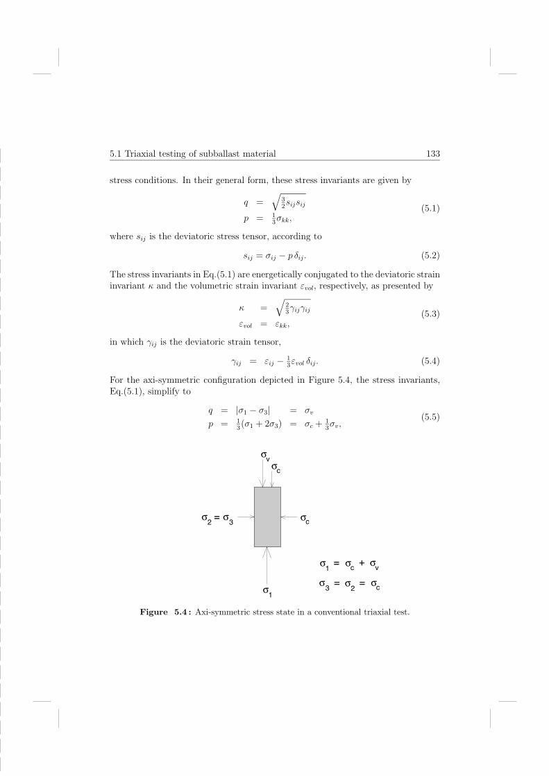
5.1 Triaxial testing of subballast material 133
stress conditions. In their general form, these stress invariants are given by
q =√
32sijsij
p = 13σkk,
(5.1)
where sij is the deviatoric stress tensor, according to
sij = σij − p δij. (5.2)
The stress invariants in Eq.(5.1) are energetically conjugated to the deviatoric straininvariant κ and the volumetric strain invariant εvol, respectively, as presented by
κ =√
23γijγij
εvol = εkk,(5.3)
in which γij is the deviatoric strain tensor,
γij = εij − 13εvol δij. (5.4)
For the axi-symmetric configuration depicted in Figure 5.4, the stress invariants,Eq.(5.1), simplify to
q = |σ1 − σ3| = σv
p = 13(σ1 + 2σ3) = σc +
13σv,
(5.5)
σv
σc
cσ
cσσ
1σ
σ
v
σ3 2
σc
σ
= +
= =σ
1
σ3
=2
Figure 5.4 : Axi-symmetric stress state in a conventional triaxial test.
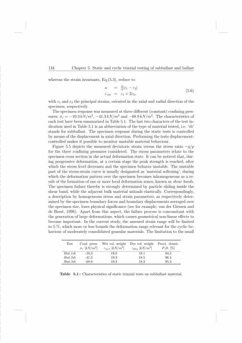
134 Chapter 5. Static and cyclic triaxial testing of subballast and ballast
whereas the strain invariants, Eq.(5.3), reduce to
κ = 23|ε1 − ε3|
εvol = ε1 + 2ε3,(5.6)
with ε1 and ε3 the principal strains, oriented in the axial and radial direction of thespecimen, respectively.The specimen response was measured at three different (constant) confining pres-
sures; σc = −10.3 kN/m2, −41.3 kN/m2 and −68.9 kN/m2. The characteristics ofeach test have been summarised in Table 5.1. The last two characters of the test in-dication used in Table 5.1 is an abbreviation of the type of material tested, i.e. ’sb’stands for subballast. The specimen response during the static tests is controlledby means of the displacement in axial direction. Performing the tests displacement-controlled makes it possible to monitor unstable material behaviour.Figure 5.5 depicts the measured deviatoric strain versus the stress ratio −q/p
for the three confining pressures considered. The stress parameters relate to thespecimen cross section in the actual deformation state. It can be noticed that, dur-ing progressive deformation, at a certain stage the peak strength is reached, afterwhich the stress level decreases and the specimen behaves unstable. The unstablepart of the stress-strain curve is usually designated as ’material softening’, duringwhich the deformation pattern over the specimen becomes inhomogeneous as a re-sult of the formation of one or more local deformation zones, known as shear bands.The specimen failure thereby is strongly determined by particle sliding inside theshear band, while the adjacent bulk material unloads elastically. Correspondingly,a description by homogeneous stress and strain parameters, as respectively deter-mined by the specimen boundary forces and boundary displacements averaged overthe specimen size, loses physical significance (see for example, van der Giessen andde Borst, 1998). Apart from this aspect, the failure process is concomitant withthe generation of large deformations, which causes geometrical non-linear effects tobecome important. In the current study, the assessed strain range will be limitedto 5 %, which more or less bounds the deformation range relevant for the cyclic be-haviour of moderately consolidated granular materials. The limitation to the small
Test Conf. press. Wet vol. weight Dry vol. weight Proct. densit.σc [kN/m2] γwet [kN/m3] γdry [kN/m3] P.D. [%]
Stat.1sb -10.3 19.0 18.1 94.3Stat.2sb -41.3 19.3 18.5 96.4Stat.3sb -68.9 19.3 18.3 95.3
Table 5.1 : Characteristics of static triaxial tests on subballast material.

5.1 Triaxial testing of subballast material 135
strain range justifies the use of a linear deformation theory and the assumptionthat the stress and deformation pattern remain (approximately) homogeneous overthe specimen.It can be noted that the three stress-strain curves in Figure 5.5 show a close cor-
respondence. This implies that for the considered confining pressures the specimenfailure characteristics can be approximated by a criterion that is linear in the p− qplane, such as the Mohr-Coulomb criterion or the Drucker-Prager criterion (seefor example, Vardoulakis and Sulem, 1995). Figure 5.6 gives the result of a linearregression that has been applied to the measured peak strengths. The regressionline has been constructed by requiring that it passes the origin, thus characterizinga non-cohesive material. Apparently, the slope of the regression line agrees witha peak strength of (−q/p)stat,max = 1.68. In agreement with the Mohr-Coulombor the Drucker-Prager criterion, this peak strength relates to a friction angle ofφstat,max = 41.It is acknowledged that at confining pressures higher than those considered here
the failure envelope may manifest a curved character in the p − q plane (Tat-suoka and Ishihara, 1974; Lade, 1977). A curved failure envelope suggests thatthe mechanisms of volumetric compaction and particle crushing substantially markthe mechanical behaviour of the specimen. For obvious reasons, the applicationof a linear frictional failure criterion then gives a less accurate prediction of themeasured failure response.In Figure 5.7, the deviatoric strain measured in the 0-5 % strain range has been
depicted versus the volumetric strain. The strain parameters have been computedby using Eq.(5.6), in which the principal strains ε1 and ε3 have been derived fromthe measured vertical displacement and circumferential displacement, respectively.The curves start with a negative tangential slope representing compaction, whichgradually evolves into a positive tangential slope representing dilation. The individ-ual curves appear to be somewhat different, in a sense that an increased confiningpressure decreases the amount of dilation produced during failure. This effect hasalso been reported by other investigators, see for example Raymond and Davies,1978, and implies that an increase of the hydrostatic pressure shifts the deformationcharacteristics at failure from the dilation regime towards the compaction regime.The minor wrinkles appearing at the onset of the response were caused by a local,temporarily circumferential stiffening, resulting from the bending resistance of thepieces of Teflon tubing surrounding the Teflon-coated steel cable. For subsequenttests, this problem was solved by cutting the Teflon tubing into smaller pieces.
5.1.3 Cyclic triaxial tests
After the above-mentioned static tests were completed, cyclic tests were carriedout at two different (constant) confining pressures; σc = −41.3 kN/m2 and σc =

136 Chapter 5. Static and cyclic triaxial testing of subballast and ballast
Deviatoric strain κ [-]
0.00 0.02 0.04 0.06 0.08 0.10 0.12 0.14
Str
ess r
atio
-q
/ p
[
-]
0.0
0.5
1.0
1.5
2.0
2.5
(1)
(2)
(3)
(1) : Stat.1sb, σc= -10.3 kN/m2
(2) : Stat.2sb, σc= -41.3 kN/m2
(3) : Stat.3sb, σc= -68.9 kN/m2
Figure 5.5: Static response of subballast material. Stress ratio −q/p versus the totaldeviatoric strain κ for various confining pressures σc.
Hydrostatic stress p [kN/m2]
-200-175-150-125-100-75-50-250
De
via
toric s
tre
ss
q
[kN
/m2 ]
0
50
100
150
200
250
300
Stat.1sb
Stat.2sb
Stat.3sb
(-q/p)stat,max = 1.68
Measured peak strength
Linear regression through origin
Figure 5.6: Static response of subballast material. Peak strength in the p − q plane;measured values and corresponding linear regression.

5.1 Triaxial testing of subballast material 137
Deviatoric strain κ [-]
0.00 0.01 0.02 0.03 0.04 0.05
Volu
metr
ic s
train
ε v
ol
[-]
-0.02
-0.01
0.00
0.01
0.02
0.03
0.04
0.05
(1)
(2)
(3)
(1) : Stat.1sb, σc= -10.3 kN/m2
(2) : Stat.2sb, σc= -41.3 kN/m2
(3) : Stat.3sb, σc= -68.9 kN/m2
Figure 5.7: Static response of subballast material. Total volumetric strain εvol versustotal deviatoric strain κ for various confining pressures σc.
−68.9 kN/m2. At both confining pressures, the specimen response was measuredduring one million load cycles, at four different cyclic stress levels, resulting in thetotal of eight tests. The cyclic loading was applied in the axial direction of thespecimen, where each load cycle returns to full unloading, as representative for atrain axle passage. The cyclic tests were performed in a load-controlled fashion,using a periodic positive full-sine signal with a frequency of 5 Hz. A comparisonwith preliminary tests conducted at lower frequencies revealed that at 5 Hz themass inertia effects of the specimen were negligibly small, so that the materialresponse may be characterised as ’quasi-static’. The data storage occurred afterprescribed loading intervals, where each reading was performed over one individualload cycle. During such a load cycle, the displacements in axial direction and radialdirection were read 100 times, where the maximum and minimum value over thetotal amount of readings were assumed to be equal to the total displacement andthe permanent displacement, respectively.
The stress configuration for the cyclic tests is similar to that for the static tests,see Figure 5.4, though the vertical stress σv now is composed of a small static partand a cyclic part; σv = σstat + σcyc. The static part is necessary for maintainingcontact between the hydraulic load actuator and the specimen, which was achieved

138 Chapter 5. Static and cyclic triaxial testing of subballast and ballast
by applying a relatively small loading of 100N . The cyclic part varies between zeroand a specific fraction n of the static failure load (−q/p)stat,max. Accordingly, n isdenoted as the ’relative cyclic stress’, and can be expressed as
n =(−q/p)cyc
(−q/p)stat,max
, (5.7)
with (−q/p)cyc the stress amplitude for an individual load cycle. For the subballastmaterial the value of (−q/p)stat,max equals 1.68, see Figure 5.6. In Table 5.2 thecharacteristics for the cyclic triaxial tests are collected.Figures 5.8 and 5.9 show the measured deviatoric strain κ versus the logarithm
of the number of load cycles N for the two confining pressures considered. Thecurves consist of two lines, the solid line reflecting the total deformation and thedashed line reflecting the permanent deformation. Trivially, the difference betweenthe two lines equals the elastic deformation. It is evident that an increasing cyclicstress level n causes the total deviatoric deformation to increase, where the growthof the deviatoric deformation is mainly governed by the permanent deformationcomponent. The response characteristics under both confining pressures are aboutthe same, indicating that the cyclic development of the deviatoric strain may beobjectively characterised by the relative cyclic stress n, or analogously, by the cyclicstress level (−q/p)cyc.In Figures 5.10 and 5.11 the cyclic evolution of the volumetric strain is plotted
for the two confining pressures considered. Again, the solid line represents thetotal deformation and the dashed line represents the permanent deformation. Ap-parently, during the first 100 to 1000 load cycles both lines grow steadily towardseach other, which implies that the elastic volumetric deformation decreases and thegranular material becomes stiffer. In the literature, this phase is regularly referred
Test Conf. press. Rel. cyc. stress Wet vol. weight Dry vol. weight Proct. densit.σc [kN/m2] n [−] γwet [kN/m3] γdry [kN/m3] P.D. [%]
Cyc.1sb -41.3 0.495 19.2 18.5 96.4Cyc.2sb -41.3 0.845 19.3 18.4 95.8Cyc.3sb -41.3 0.960 19.1 18.4 95.8Cyc.4sb -41.3 0.995 19.3 18.4 95.8Cyc.5sb -68.9 0.545 19.3 18.5 96.4Cyc.6sb -68.9 0.821 19.4 18.6 96.9Cyc.7sb -68.9 0.950 19.4 18.6 96.9Cyc.8sb -68.9 0.975 19.3 18.5 96.4
Table 5.2 : Characteristics of one million load cycle tests on subballast material.

5.1 Triaxial testing of subballast material 139
Number of load cycles N [-]
1e+0 1e+1 1e+2 1e+3 1e+4 1e+5 1e+6
Devia
toric s
train
κ,
κp
[ -]
0.00
0.01
0.02
0.03
0.04
0.05
0.06
(4)
(3)
(2)
(1)
(1) : Cyc.1sb, n=0.495
(2) : Cyc.2sb, n=0.845
(3) : Cyc.3sb, n=0.960
(4) : Cyc.4sb, n=0.995
σc = -41.3 kN/m2
Figure 5.8: Cyclic response of subballast material. Evolution of total deviatoric strain κ(solid line) and permanent deviatoric strain κp (dashed line) with load cycles N . Variouscyclic stress levels n, where the confining pressure equals σc = −41.3 kN/m2.
Number of load cycles N [-]
1e+0 1e+1 1e+2 1e+3 1e+4 1e+5 1e+6
De
via
toric s
tra
in
κ , κ
p
[ -]
0.00
0.01
0.02
0.03
0.04
0.05
0.06
(1)
(2)
(3)
(4)(4) : Cyc.8sb, n=0.975
(3) : Cyc.7sb, n=0.950
(2) : Cyc.6sb, n=0.821
(1) : Cyc.5sb, n=0.545 σc = -68.9 kN/m2
Figure 5.9: Cyclic response of subballast material. Evolution of total deviatoric strain κ(solid line) and permanent deviatoric strain κp (dashed line) with load cycles N . Variouscyclic stress levels n, where the confining pressure equals σc = −68.9 kN/m2.

140 Chapter 5. Static and cyclic triaxial testing of subballast and ballast
Number of load cycles N [-]
1e+0 1e+1 1e+2 1e+3 1e+4 1e+5 1e+6
Volu
metr
ic s
train
ε v
ol ,
εp
vol
[-]
-0.04
-0.03
-0.02
-0.01
0.00
(1)
(4)(2)
(3)
σc = -41.3 kN/m2
(1) : Cyc.1sb, n=0.495
(4) : Cyc.4sb, n=0.995
(2) : Cyc.2sb, n=0.845
(3) : Cyc.3sb, n=0.960
Figure 5.10: Cyclic response of subballast material. Evolution of total volumetricstrain εvol (solid line) and permanent volumetric strain εp
vol (dashed line) with load cyclesN . Various cyclic stress levels n, where the confining pressure equals σc = −41.3 kN/m2.
Number of load cycles N [-]
1e+0 1e+1 1e+2 1e+3 1e+4 1e+5 1e+6
Vo
lum
etr
ic s
tra
in
ε vol ,
εp
vol
[-]
-0.04
-0.03
-0.02
-0.01
0.00
(1) : Cyc.5sb, n=0.545
(2) : Cyc.6sb, n=0.821
(3) : Cyc.7sb, n=0.950
(4) : Cyc.8sb, n=0.975
(1)
(4)
(2)
(3)
σc = -68.9 kN/m2
Figure 5.11: Cyclic response of subballast material. Evolution of total volumetricstrain εvol (solid line) and permanent volumetric strain εp
vol (dashed line) with load cyclesN . Various cyclic stress levels n, where the confining pressure equals σc = −68.9 kN/m2.
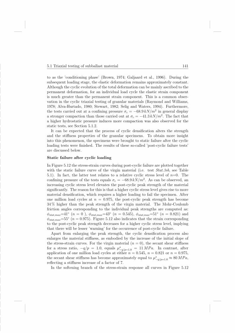
5.1 Triaxial testing of subballast material 141
to as the ’conditioning phase’ (Brown, 1974; Galjaard et al., 1996). During thesubsequent loading stage, the elastic deformation remains approximately constant.Although the cyclic evolution of the total deformation can be mainly ascribed to thepermanent deformation, for an individual load cycle the elastic strain componentis much greater than the permanent strain component. This is a common obser-vation in the cyclic triaxial testing of granular materials (Raymond and Williams,1978; Alva-Hurtado, 1980; Stewart, 1982; Selig and Waters, 1994). Furthermore,the tests carried out at a confining pressure σc = −68.9 kN/m2 in general displaya stronger compaction than those carried out at σc = −41.3 kN/m2. The fact thata higher hydrostatic pressure induces more compaction was also observed for thestatic tests, see Section 5.1.2.It can be expected that the process of cyclic densification alters the strength
and the stiffness properties of the granular specimens. To obtain more insightinto this phenomenon, the specimens were brought to static failure after the cyclicloading tests were finished. The results of these so-called ’post-cyclic failure tests’are discussed below.
Static failure after cyclic loading
In Figure 5.12 the stress-strain curves during post-cyclic failure are plotted togetherwith the static failure curve of the virgin material (i.e. test Stat.3sb, see Table5.1). In fact, the latter test relates to a relative cyclic stress level of n=0. Theconfining pressure of the tests equals σc = −68.9 kN/m2. As can be observed, anincreasing cyclic stress level elevates the post-cyclic peak strength of the materialsignificantly. The reason for this is that a higher cyclic stress level gives rise to morematerial densification, which requires a higher loading to fail the specimen. Afterone million load cycles at n = 0.975, the post-cyclic peak strength has become34% higher than the peak strength of the virgin material. The Mohr-Coulombfriction angles corresponding to the individual peak strengths are computed as:φstat,max=41
(n = 0 ), φstat,max=43 (n = 0.545), φstat,max=51
(n = 0.821) andφstat,max=55
(n = 0.975). Figure 5.12 also indicates that the strain correspondingto the post-cyclic peak strength decreases for a higher cyclic stress level, implyingthat there will be lesser ’warning’ for the occurrence of post-cyclic failure.Apart from enlarging the peak strength, the cyclic densification process also
enlarges the material stiffness, as embodied by the increase of the initial slope ofthe stress-strain curves. For the virgin material (n = 0), the secant shear stiffnessfor a stress ratio, −q/p = 1.0, equals µs
−q/p=1.0 = 11MPa. In contrast, afterapplication of one million load cycles at either n = 0.545, n = 0.821 or n = 0.975,the secant shear stiffness has become approximately equal to µs
−q/p=1.0 ≈ 80MPa,reflecting a stiffness increase of a factor of 7.In the softening branch of the stress-strain response all curves in Figure 5.12

142 Chapter 5. Static and cyclic triaxial testing of subballast and ballast
Deviatoric strain κ [-]
0.00 0.02 0.04 0.06 0.08 0.10 0.12 0.14
Str
ess r
atio
-q
/ p
[
-]
0.0
0.5
1.0
1.5
2.0
2.5
(1)
(2)
(3)
(4)
(1) : Virgin material, n=0(2) : After one million load cycles at n=0.545
(3) : After one million load cycles at n=0.821(4) : After one million load cycles at n=0.975
σc = -68.9 kN/m2
Figure 5.12: Static response of subballast material after pre-loading at various cyclicstress levels n. Stress ratio −q/p versus the total deviatoric strain κ, where the confiningpressure equals σc = −68.9 kN/m2.
Deviatoric strain κ [-]
0.00 0.01 0.02 0.03 0.04 0.05
Vo
lum
etr
ic s
tra
in
ε vol
[ -]
-0.02
-0.01
0.00
0.01
0.02
0.03
0.04
0.05
(1)
(2)
(4)(3)
(1) : Virgin material, n=0(2) : After one million load cycles at n=0.545(3) : After one million load cycles at n=0.821(4) : After one million load cycles at n=0.975
σc = -68.9 kN/m2
Figure 5.13: Static response of subballast material after pre-loading at various cyclicstress levels n. Total volumetric strain εvol versus the total deviatoric strain κ, where theconfining pressure equals σc = −68.9 kN/m2.

5.1 Triaxial testing of subballast material 143
approach each other. This is expected, because at large deformations the failureprocess is strongly governed by local shear bands, for which the strength is indepen-dent of the compaction level of the adjacent bulk material. Also, for an increasedcyclic stress level the tangent of the softening branch becomes steeper at the onsetof softening, which corresponds to the emergence of a more prominent localisationzone.
The deformation characteristics for the post-cyclic failure tests have been plottedin Figure 5.13. It can be seen that the transition from material compaction intomaterial dilation occurs faster if the stress level during the cyclic loading stage ishigher. Because the onset of dilation is a precursor to frictional failure, a fastertransition into dilation relates to a smaller deformation necessary for reaching post-cyclic failure.
Test repeatability and response to five million load cycles
The cyclic loading tests discussed previously were ended when the number of loadcycles exceeded one million. As exemplified, the deformation rate measured duringthese tests generally decreased at an increased number of load cycles. It can beexpected that this tendency proceeds when the number of load cycles becomeslarger than one million, though it is important to verify this, since in railwaypractice a maintenance period may span more train passages than the equivalentof one million load cycles. For this reason, the number of load cycles in a cyclictest was increased to five million. Because of the large time-consumption of a fivemillion load cycles test, it was decided to restrict the number of tests to one.
The characteristics of the five million load cycles test are presented in Table 5.3.It can be observed that the applied cyclic stress level is close to the failure strengthof the virgin material. Since the characteristics of test Cyc.9sb (see Table 5.3)closely resemble those of test Cyc.3sb (see Table 5.2), these tests are compared inorder to check the test repeatability. Figure 5.14 depicts the cyclic evolution of thedeviatoric strain for the two tests, whereas Figure 5.15 depicts the cyclic evolution ofthe volumetric strain. It can be noticed that the trend of the deformation sketchedin these figures is very much the same for both tests. In a quantitative sense thereare some differences, in particular with respect to the evolution of the volumetric
Test Conf. press. Rel. cyc. stress Wet vol. weight Dry vol. weight Proct. densit.σc [kN/m2] n [−] γwet [kN/m3] γdry [kN/m3] P.D. [%]
Cyc.9sb -41.3 0.98 19.3 18.6 96.9
Table 5.3 : Characteristics of five million load cycles test on subballast material.

144 Chapter 5. Static and cyclic triaxial testing of subballast and ballast
Number of load cycles N [-]
1e+0 1e+1 1e+2 1e+3 1e+4 1e+5 1e+6 1e+7
Devia
toric s
train
κ
, κp
[
-]
0.00
0.01
0.02
0.03
0.04
0.05
0.06
(2)
(1)
(1) : 1 million load cycles test, Cyc.3sb
(2) : 5 million load cycles test, Cyc.9sb
σc = -41.3 kN/m2
Figure 5.14: Cyclic response of subballast material. Representation of test repeatabil-ity and response characteristics up to five million load cycles. Evolution of total deviatoricstrain κ (solid line) and permanent deviatoric strain κp (dashed line) with load cycles N .The confining pressure equals σc = −41.3 kN/m2.
Number of load cycles N [-]
1e+0 1e+1 1e+2 1e+3 1e+4 1e+5 1e+6 1e+7
Vo
lum
etr
ic s
tra
in
ε vol ,
εp
vol
[ -]
-0.04
-0.03
-0.02
-0.01
0.00
(1)(2)
(1) : 1 million load cycles test, Cyc.3sb
(2) : 5 million load cycles test, Cyc.9sb
σc = -41.3 kN/m2
Figure 5.15: Cyclic response of subballast material. Representation of test repeata-bility and response characteristics up to five million load cycles. Evolution of total vol-umetric strain εvol (solid line) and permanent volumetric strain εp
vol (dashed line) withload cycles N . The confining pressure equals σc = −41.3 kN/m2.

5.2 Triaxial testing of ballast material 145
strain. These discrepancies may be due to small dissimilarities in the applied cyclicloading level, and the Proctor density of the specimens, see Tables 5.2 and 5.3.
For test Cyc.9sb, the deformation generated between one million and five millionload cycles is obviously very small compared to the deformation generated over thecomplete loading period. As expected, the deformation rate progressively decreasesduring the complete loading period, even though the cyclic stress level is very closeto the static failure level of the virgin material.
5.2 Triaxial testing of ballast material
This section treats the testing program for the ballast material. Because of thesimilarities with the testing program for the subballast material, the discussion ofthe test procedure and the test results will be presented in a rather concise manner.
5.2.1 Experimental set-up and test procedure
The principle of the triaxial load apparatus used for the ballast testing is identicalto that used for the subballast testing, see Figure 5.2. However, since the averageparticle size of a ballast gradation is larger than that of a subballast gradation, thesize of the current triaxial load apparatus is bigger in order to prevent a negativeinfluence of size effects. In the triaxial load apparatus the nominal diameter of thecylindrical specimen equals D = 254mm, whereas the nominal height is equal toH = 645mm. This yields an aspect ratio of H/D = 2.53. The largest grain size inthe uniformly-graded ballast material is d = 38mm, see Figure 5.1, correspondingto a specimen diameter to grain size ratio of D/d ≈ 7. The ballast material fulfillsthe requirements of a gradation number 4, as specified in the AREA Manual forRailway Engineering (AREA, 1988). Because ballast consists of relatively coarseparticles, the material has a high moisture permeability, so that it is unnecessaryto moisten the ballast during the specimen preparation. The specimen preparationoccurred by stacking and compacting eight layers of equal thickness, where eachlayer was tamped 40 strokes with a steel rod. This procedure is supposed to mimicthe initial compaction level of the traprock ballast used in the Colorado test-track(Selig et al., 1981). The specimen was enclosed by a latex membrane of 0.76mmthickness that was manually cut from a roll and subsequently glued together. Themembrane was chosen somewhat thicker than that used for the subballast testing,in order to avoid membrane puncturing by the sharp edges of the ballast particles.Because of the large specimen height H, three circumferential displacement deviceswere attached to the specimen, at respectively H/3, H/2 and 2H/3, see Figure5.16.

146 Chapter 5. Static and cyclic triaxial testing of subballast and ballast
5.2.2 Static triaxial tests
The properties of the static ballast tests are collected in Table 5.4. The threeconfining pressures that were applied are equal to those applied for the subballasttesting. The static tests were carried out in a displacement-controlled fashion. Thestress-strain curves measured at the various confining pressures have been plotted inthe Figures 5.17, 5.18 and 5.19. Each figure consists of three curves, correspondingto the circumferential displacement measurements at H/3, H/2 and 2H/3. It is
Figure 5.16: Three circumferential displacement devices attached to a ballast specimen.

5.2 Triaxial testing of ballast material 147
Test Conf. press. Dry vol. weightσc [kN/m2] γdry [kN/m3]
Stat.1b -10.3 16.1Stat.2b -41.3 17.0Stat.3b -68.9 16.2
Table 5.4 : Characteristics of static triaxial tests on ballast material.
obvious that the three stress-strain curves in each figure are nearly identical. Thesmall spikes emerging in the response are due to instantaneous sliding of individualparticles. These local instabilities are registered at the specimen level because theratio between the average ballast particle size and the specimen size is relativelylarge.
In contrast with the subballast material, material softening is not observed forthe ballast material. The absence of material softening may be ascribed to theuniform character of the particle size distribution of the ballast, see Figure 5.1. Infact, a uniformly-graded material is less susceptible to compaction than a broadly-graded material, in which smaller particles are forced inside the spaces created bybigger particles. As a result, a uniform particle gradation subjected to a uniformstress reveals a more or less uniform deformation pattern. The distinction between’uniform failure’ and ’non-uniform failure’ has been made previously by Lade (1982),in which non-uniform failure by one or more local shear bands was named ’linefailure’ and failure by (approximately) uniform particle sliding was named ’zonefailure’. When zone failure occurs, material softening remains absent, becauseuniform particle sliding excludes material parts that unload elastically.
In Figure 5.20 the peak strengths of the three stress-strain responses have beenplotted in the p− q plane. As for the subballast, a linear criterion that passes theorigin in the p − q plane gives an accurate approximation of the frictional failurelevel. The peak strength, (−q/p)stat,max = 1.98, is somewhat higher than that of thesubballast material, and relates to a Mohr-Coulomb friction angle of φstat,max = 48.In Figures 5.21, 5.22 and 5.23 the static deformation characteristics measured
at the various confining pressures have been depicted. The three figures actuallyreveal an identical trend; initially the material displays some compaction, whichevolves relatively fast into dilation. As for the subballast material, for an increasingconfining pressure the amount of dilation decreases. The quantitative differencesbetween the deformation curves depicted in the individual figures indicate thatthe strain is not completely homogeneous over the specimen height H. A possibleexplanation for this inhomogeneity may be the presence of some friction at thespecimen top and bottom, which manifested itself during the experiments by minor
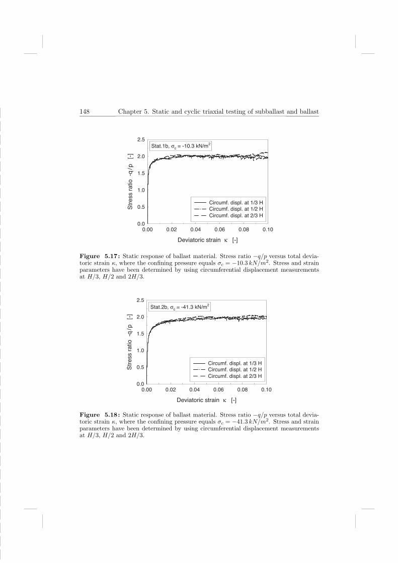
148 Chapter 5. Static and cyclic triaxial testing of subballast and ballast
Deviatoric strain κ [-]
0.00 0.02 0.04 0.06 0.08 0.10
Str
ess r
atio
-q
/ p
[
-]
0.0
0.5
1.0
1.5
2.0
2.5
Circumf. displ. at 1/3 HCircumf. displ. at 1/2 HCircumf. displ. at 2/3 H
Stat.1b, σc = -10.3 kN/m2
Figure 5.17: Static response of ballast material. Stress ratio −q/p versus total devia-toric strain κ, where the confining pressure equals σc = −10.3 kN/m2. Stress and strainparameters have been determined by using circumferential displacement measurementsat H/3, H/2 and 2H/3.
Deviatoric strain κ [-]
0.00 0.02 0.04 0.06 0.08 0.10
Str
ess r
atio -q
/ p [
-]
0.0
0.5
1.0
1.5
2.0
2.5
Circumf. displ. at 1/3 HCircumf. displ. at 1/2 HCircumf. displ. at 2/3 H
Stat.2b, σc = -41.3 kN/m2
Figure 5.18: Static response of ballast material. Stress ratio −q/p versus total devia-toric strain κ, where the confining pressure equals σc = −41.3 kN/m2. Stress and strainparameters have been determined by using circumferential displacement measurementsat H/3, H/2 and 2H/3.

5.2 Triaxial testing of ballast material 149
Deviatoric strain κ [-]
0.00 0.02 0.04 0.06 0.08 0.10
Str
ess r
atio -q
/ p [
-]
0.0
0.5
1.0
1.5
2.0
2.5
Circumf. displ. at 1/3 HCircumf. displ. at 1/2 HCircumf. displ. at 2/3 H
Stat.3b, σc = -68.9 kN/m2
Figure 5.19: Static response of ballast material. Stress ratio −q/p versus total devia-toric strain κ, where the confining pressure equals σc = −68.9 kN/m2. Stress and strainparameters have been determined by using circumferential displacement measurementsat H/3, H/2 and 2H/3.
Hydrostatic stress p [kN/m2]
-250-225-200-175-150-125-100-75-50-250
De
via
toric s
tre
ss
q
[ kN
/m2 ]
0
50
100
150
200
250
300
350
400
450
(-q/p)stat,max = 1.98
Stat.1b
Stat.2b
Stat.3b
Measured peak strength
Linear regression through origin
Figure 5.20: Static response of ballast material. Peak strength in the p − q plane;measured values and corresponding linear regression.

150 Chapter 5. Static and cyclic triaxial testing of subballast and ballast
Deviatoric strain κ [-]
0.00 0.01 0.02 0.03 0.04 0.05
Vo
lum
etr
ic s
tra
in
ε vo
l [ -
]
-0.02
-0.01
0.00
0.01
0.02
0.03
0.04
0.05Circumf. displ. at 1/3 HCircumf. displ. at 1/2 HCircumf. displ. at 2/3 H
Stat.1b, σc = -10.3 kN/m2
Figure 5.21: Static response of ballast material. Total volumetric strain εvol versustotal deviatoric strain κ, where the confining pressure equals σc = −10.3 kN/m2. Stressand strain parameters have been determined by using circumferential displacement mea-surements at H/3, H/2 and 2H/3.
Deviatoric strain κ [-]
0.00 0.01 0.02 0.03 0.04 0.05
Vo
lum
etr
ic s
tra
in
ε vo
l [ -
]
-0.02
-0.01
0.00
0.01
0.02
0.03
0.04
0.05Circumf. displ. at 1/3 HCircumf. displ. at 1/2 HCircumf. displ. at 2/3 H
Stat.2b, σc = -41.3 kN/m2
Figure 5.22: Static response of ballast material. Total volumetric strain εvol versustotal deviatoric strain κ, where the confining pressure equals σc = −41.3 kN/m2. Stressand strain parameters have been determined by using circumferential displacement mea-surements at H/3, H/2 and 2H/3.

5.2 Triaxial testing of ballast material 151
Deviatoric strain κ [-]
0.00 0.01 0.02 0.03 0.04 0.05
Vo
lum
etr
ic s
tra
in
ε vo
l [ -
]
-0.02
-0.01
0.00
0.01
0.02
0.03
0.04
0.05
Circumf. displ. at 1/3 HCircumf. displ. at 1/2 HCircumf. displ. at 2/3 H
Stat.3b, σc = -68.9 kN/m2
Figure 5.23: Static response of ballast material. Total volumetric strain εvol versustotal deviatoric strain κ, where the confining pressure equals σc = −68.9 kN/m2. Stressand strain parameters have been determined by using circumferential displacement mea-surements at H/3, H/2 and 2H/3.
specimen bulging. Most likely, this effect could have been somewhat reduced byapplying a lubricant at the specimen ends (Hjortnaes-Pedersen and Molenkamp,1982).
5.2.3 Cyclic triaxial tests
The cyclic loading tests on the ballast were performed in a load-controlled fashion,at a frequency of 5Hz, where the specimen response was periodically registeredduring one million load cycles. In Table 5.5 the characteristics for the cyclic testsare presented. It should be realised that the relative cyclic stress n, as presentedby Eq.(5.7), here relates to a static failure level of (−q/p)stat,max = 1.98, see Figure5.20.
In Figures 5.24 and 5.25 the cyclic evolution of the deviatoric strain has beensketched for the two confining pressures considered. The stress and strain pa-rameters used in the presentation of the results correspond to the average of thecircumferential displacement measurements at H/3, H/2 and 2H/3. The curvesshow a trend that is comparable to that measured for the subballast, see Figures 5.8

152 Chapter 5. Static and cyclic triaxial testing of subballast and ballast
Test Conf. press. Rel. cyc. stress Dry vol. weightσc [kN/m2] n [−] γdry [kN/m3]
Cyc.1b -41.3 0.510 16.3Cyc.2b -41.3 0.822 16.3Cyc.3b -41.3 0.964 16.6Cyc.4b -41.3 0.979 16.6Cyc.5b -68.9 0.508 16.5Cyc.6b -68.9 0.817 16.8Cyc.7b -68.9 0.958 16.6Cyc.8b -68.9 0.973 16.7
Table 5.5 : Characteristics of one million load cycle tests on ballast material.
and 5.9. It can further be observed that at lower cyclic stress levels, n < 0.82, thepermanent deformation rate at one million load cycles has become negligibly small.In other words, the cyclic response has become (almost) elastic. This phenomenonis known as ’shakedown’.
The cyclic evolution of the volumetric strain, depicted in Figures 5.26 and 5.27,shows that the ballast material is less susceptible to compaction than the subbal-last material, see Figures 5.10 and 5.11. As explained before, the low compactionsusceptibility stems from the uniform particle gradation of the ballast material. Atstress levels close to failure, the volumetric strain rate during the initial loadingphase is slightly positive, representing dilation. At about one thousand load cyclesthe dilation changes into compaction, after which the compaction level increasesmore or less linearly with the logarithm of the number of load cycles.
In general, material compaction may be the result of particle rearrangement, par-ticle crushing, or a combination of both mechanisms. Sieving procedures conductedafter the tests were finished only revealed a small amount of particle breakage,which suggests that material compaction is driven here mainly by particle rear-rangement. This finding is supported by additional static oedometer tests1 (Suiker,1999), which showed that for the current ballast material the hydrostatic stress atwhich particle crushing is initiated equals p = −350 kN/m2. This stress level isconsiderably higher than the maximum hydrostatic stress applied in the triaxialtests; p = −193 kN/m2, see Figure 5.20.
Static failure after cyclic loading
The post-cyclic failure behaviour of the ballast is illustrated by the stress-straincurves in Figure 5.28 and the deformation curves in Figure 5.29. As for the subbal-
1An oedometer test also sometimes is referred to as a ’compressometer test’.

5.2 Triaxial testing of ballast material 153
Number of load cycles N [-]
1e+0 1e+1 1e+2 1e+3 1e+4 1e+5 1e+6
De
via
toric s
tra
in
κ ,
κp
[-]
0.00
0.01
0.02
0.03
0.04
0.05
0.06
(4)
(3)
(2)
(1) : Cyc.1b, n=0.510(2) : Cyc.2b, n=0.822(3) : Cyc.3b, n=0.964(4) : Cyc.4b, n=0.979
(1)
σc = -41.3 kN/m2
Figure 5.24: Cyclic response of ballast material. Evolution of total deviatoric strain κ(solid line) and permanent deviatoric strain κp (dashed line) with load cycles N . Variouscyclic stress levels n, where the confining pressure equals σc = −41.3 kN/m2.
Number of load cycles N [-]
1e+0 1e+1 1e+2 1e+3 1e+4 1e+5 1e+6
De
via
toric s
tra
in
κ ,
κp
[-]
0.00
0.01
0.02
0.03
0.04
0.05
0.06
(4)
(3)
(2)
(1)
(1) : Cyc.5b, n=0.508(2) : Cyc.6b, n=0.817
(3) : Cyc.7b, n=0.958(4) : Cyc.8b, n=0.973
σc = -68.9 kN/m2
Figure 5.25: Cyclic response of ballast material. Evolution of total deviatoric strain κ(solid line) and permanent deviatoric strain κp (dashed line) with load cycles N . Variouscyclic stress levels n, where the confining pressure equals σc = −68.9 kN/m2.

154 Chapter 5. Static and cyclic triaxial testing of subballast and ballast
Number of load cycles N [-]
1e+0 1e+1 1e+2 1e+3 1e+4 1e+5 1e+6
Vo
lum
etr
ic s
tra
in
ε vo
l , ε
pvo
l [
-]
-0.03
-0.02
-0.01
0.00
0.01
0.02
0.03
(1)
(4)
(2)
(3)
(1) : Cyc.1b, n=0.510
(4) : Cyc.4b, n=0.979
(2) : Cyc.2b, n=0.822
(3) : Cyc.3b, n=0.964σc = -41.3 kN/m
2
Figure 5.26: Cyclic response of ballast material. Evolution of total volumetric strainεvol (solid line) and permanent volumetric strain εp
vol (dashed line) with load cycles N .Various cyclic stress levels n, where the confining pressure equals σc = −41.3 kN/m2.
Number of load cycles N [-]
1e+0 1e+1 1e+2 1e+3 1e+4 1e+5 1e+6
Volu
metr
ic s
train
ε v
ol ,
εp
vo
l [ -
]
-0.03
-0.02
-0.01
0.00
0.01
0.02
0.03
(1)
(4)
(2)(3)
(2) : Cyc.6b, n=0.817(1) : Cyc.5b, n=0.508
(3) : Cyc.7b, n=0.958(4) : Cyc.8b, n=0.973 σc = -68.9 kN/m
2
Figure 5.27: Cyclic response of ballast material. Evolution of total volumetric strainεvol (solid line) and permanent volumetric strain εp
vol (dashed line) with load cycles N .Various cyclic stress levels n, where the confining pressure equals σc = −68.9 kN/m2.

5.2 Triaxial testing of ballast material 155
Test Conf. press. Rel. cyc. stress Dry vol. weightσc [kN/m2] n [−] γdry [kN/m3]
Cyc.9b -41.3 0.956 16.3
Table 5.6 : Characteristics of five million load cycles test on ballast material.
last material, the cyclic loading process increases the peak strength, the stiffness,and the static dilation of the ballast. However, the increase in peak strength is lesspronounced than for the subballast material; the static failure level obtained aftercyclic loading at n = 0.973 is only 9% higher than the static failure level of the vir-gin ballast material (n = 0). This corresponds to an increase of the Mohr-Coulombfriction angle from φstat,max = 48o (n = 0) to φstat,max = 53o (n = 0.973). The smallincrease in peak strength can be ascribed to the low compaction susceptibility ofthe ballast. This is also the reason that the relative stiffness increase of the bal-last material is smaller than that of the subballast material. More specifically, thevirgin ballast material (n = 0) has a secant shear modulus of µs
−q/p=1.0 = 33MPa
for a stress ratio −q/p = 1.0, whereas, for all cyclic stress levels considered, afterapplication of one million load cycles the secant shear modulus has become approx-imately equal to µs
−q/p=1.0 ≈ 115MPa. This corresponds to a stiffness increase ofa factor of 3.5.The responses plotted Figure 5.28 show that the spikes reflecting the sliding of
individual particles become more prominent for a higher cyclic stress level. Thiscan be explained by the fact that a higher cyclic stress level is accompanied by ahigher material densification, the effect of which may cause the stress drop duringparticle sliding to become larger.
Test repeatability and response to five million load cycles
The properties of the five million load cycles test are presented in Table 5.6. Toanalyse the test repeatability, the results are compared to those of test Cyc.3b,of which the test characteristics are given in Table 5.5. Apparently, the cyclicevolution of the deviatoric strain (Figure 5.30), as well as the cyclic evolution ofthe volumetric strain (Figure 5.31), are in reasonable agreement. The discrepanciesin the responses are believed to be mainly due to a different initial material density,which appeared to be a difficult parameter to reproduce in the testing procedure.Similar to the subballast material, the deformation produced after one million loadcycles is very small.

156 Chapter 5. Static and cyclic triaxial testing of subballast and ballast
Deviatoric strain κ [-]
0.00 0.01 0.02 0.03 0.04 0.05 0.06 0.07 0.08
Str
ess r
atio
-q
/ p
[ -
]
0.0
0.5
1.0
1.5
2.0
2.5
(1)
(2)
(3)
(4)
(1) : Virgin material, n=0(2) : After one million load cycles at n=0.508(3) : After one million load cycles at n=0.817
(4) : After one million load cycles at n=0.973
σc = -68.9 kN/m2
Figure 5.28: Static response of ballast material after pre-loading at various cyclic stresslevels n. Stress ratio −q/p versus the total deviatoric strain κ. The confining pressureequals σc = −68.9 kN/m2.
Deviatoric strain κ [-]
0.00 0.01 0.02 0.03 0.04 0.05
Vo
lum
etr
ic s
tra
in
ε vol
[-]
-0.02
-0.01
0.00
0.01
0.02
0.03
0.04
0.05
(1)
(2)
(4)
(3)
(1) : Virgin material, n=0(2) : After one million load cycles at n=0.508
(3) : After one million load cycles at n=0.817(4) : After one million load cycles at n=0.973
σc = -68.9 kN/m2
Figure 5.29: Static response of ballast material after pre-loading at various cyclic stresslevels n. Total volumetric strain εvol versus the total deviatoric strain κ. The confiningpressure equals σc = −68.9 kN/m2.

5.2 Triaxial testing of ballast material 157
Number of load cycles N [-]
1e+0 1e+1 1e+2 1e+3 1e+4 1e+5 1e+6 1e+7
De
via
toric s
tra
in
κ , κ
p
[ -]
0.00
0.01
0.02
0.03
0.04
0.05
0.06
(2)
(1)
(1) : 1 million load cycles test, Cyc.3b
(2) : 5 million load cycles test, Cyc.9b
σc = -41.3 kN/m2
Figure 5.30: Cyclic response of ballast material. Representation of test repeatabilityand response characteristics up to five million load cycles. Evolution of total deviatoricstrain κ (solid line) and permanent deviatoric strain κp (dashed line) with load cycles N .The confining pressure equals σc = −41.3 kN/m2.
Number of load cycles N [-]
1e+0 1e+1 1e+2 1e+3 1e+4 1e+5 1e+6 1e+7
Vo
lum
etr
ic s
tra
in
ε vol,
εpvol
[ -]
-0.03
-0.02
-0.01
0.00
0.01
0.02
0.03
(1)
(2)
(1) : 1 million load cycles test, Cyc.3b
(2) : 5 million load cycles test, Cyc.9b
σc = -41.3 kN/m2
Figure 5.31: Cyclic response of ballast material. Representation of test repeatabilityand response characteristics up to five million load cycles. Evolution of total volumetricstrain εvol (solid line) and permanent volumetric strain εp
vol (dashed line) with load cyclesN . The confining pressure equals σc = −41.3 kN/m2.
158 Chapter 5. Static and cyclic triaxial testing of subballast and ballast
5.3 Discussion
The elasto-plastic behaviour of a ballast and subballast material has been exploredby means of static and cyclic triaxial tests. The cyclic triaxial tests were carried outto provide insight into the deformation characteristics of these railway substructurematerials under a large number of train axle passages. The purpose of the statictests has been to identify the maximum stress level that can be applied in thecyclic tests, and to assess the strength and stiffness increase produced by the cyclicloading process. For the ballast and subballast material tested, the permanentdeformations generated by the cyclic loading initially build up rapidly, though therate of permanent deformations decreases progressively under an increasing numberof load cycles. Depending on the amplitude of the cyclic stress, after a very largenumber of load cycles (in the range of 104 < N < 106) the rate of permanentdeformation may even become negligibly small, yielding an almost fully elasticmaterial response. This phenomenon is known as ’shakedown’.
During the cyclic loading process the subballast generally compacts, even atcyclic stress levels close to the failure strength of the virgin material. The ballastmaterial also reveals a tendency to compact, though at cyclic stress levels closeto the failure strength initially some dilation occurs. Nonetheless, after about athousand load cycles the dilation changes into compaction, which signals the onsetof progressive densification.
Densification due to cyclic loading stiffens and strengthens the granular testsample. The triaxial tests revealed that the material stiffening mainly developsduring the first one hundred to one thousand load cycles, which in the literature isregularly referred to as the ’conditioning phase’. As a result of the cyclic loadingprocess, the stiffness of the subballast increased up to a factor of 7 in regard tothe stiffness of the virgin material, while for the ballast it increased up to a factorof 3.5. Furthermore, the failure strength of the subballast showed a maximumincrease of 34%, whereas the failure strength of the ballast maximally increasedby 9%. The ballast developed a relatively small increase in stiffness and failurestrength because of its low susceptibility to compaction, caused by its uniformparticle size distribution.
Although the tests showed that the application of cyclic loading may generateconsiderable permanent deformations in the sample tested, in general a substantialconsolidation of the material was achieved. For obvious reasons, track maintenanceprocedures should aim to preserve a consolidated granular substructure as much aspossible. In this respect, stoneblowing is preferable to tamping. While stoneblowingonly adds granular material to the consolidated ballast structure, during tampingthe consolidation level of the ballast is (heavily) disturbed. As a result, after atamping operation has taken place, the rate of track deterioration often ends up

5.3 Discussion 159
higher than before the tamping operation (Esveld, 1989; Selig and Waters, 1994).For both the subballast and the ballast material, the permanent deviatoric de-
formations generated under cyclic loading appear to be strongly dependent on thestress ratio (−q/p)cyc. Conversely, the permanent volumetric deformation appearsto be governed by both the stress ratio (−q/p)cyc and the hydrostatic pressure p.In other words, the generated permanent deviatoric deformations are mainly dueto frictional sliding of particles, whereas the generated permanent volumetric de-formation is due to both frictional sliding and volumetric compaction of particles.Although the current triaxial experiments do not cover all stress conditions in arailway substructure, it seems reasonable to assume that these two mechanismsgenerally mark the substructure response under a large number of train axle pas-sages. In this respect, proper simulation of track deterioration requires adequateincorporation of these mechanisms into a cyclic material model. This is done in thesubsequent chapter, where the present test results will be used for the calibrationof the cyclic material model.

160 Chapter 5. Static and cyclic triaxial testing of subballast and ballast

Chapter 6
Modelling of track deterioration
Detailed understanding of long-term deterioration of railway tracks under a largenumber of train passages and accurate prediction of corresponding maintenanceperiods necessitate the development of advanced track deterioration models. Itis important that these models include the cyclic accumulation of permanent de-formations in the granular substructure, which essentially forms the basis for theemergence of deterioration profiles of a medium to long wavelength, 3m < Λ < 50m(Esveld, 1989). In general, from the permanent deformation behaviour of the gran-ular substructure two important mechanisms can be discerned, namely (i) frictionalsliding of particles, and (ii) volumetric compaction of particles. Both deformationmechanisms are of a plastic nature, meaning that they are activated after a cer-tain stress level is exceeded, and that their magnitude remains constant as soon asunloading occurs.
Though, for an individual train axle passage, the plastic deformation causedby these mechanisms is relatively small, the cumulative effect over a (very) largenumber of train axle passages may be considerable. In this respect, a model thatsimulates the plastic deformation behaviour during each individual load cycle isunattractive, as such a model would require a vast amount of computer processingtime to calculate the deformations corresponding to common track deteriorationperiods. This problem can be overcome by employing a model that captures onlythe envelope of the maximum plastic deformations generated during the cyclicloading process, which allows to evaluate the deformation accumulation by meansof relatively large load cycle increments. In fact, a similar concept has been usedin the modelling of metal fatigue (Lemaitre and Chaboche, 1990; Peerlings et al.,2000).
The cyclic model proposed in this chapter follows the latter approach, and isderived using the classical plasticity framework as a point of departure. The incre-mental expression that is arrived at, which describes the permanent deformation

162 Chapter 6. Modelling of track deterioration
generated per cycle, follows a so-called ’overstress formulation’, similar to the over-stress formulation in the well-known viscoplastic model of Perzyna (Perzyna, 1966).The overstress formulation is applied to both frictional sliding and volumetric com-paction, by incorporating a Drucker-Prager cone that is limited in direction of thehydrostatic axis by a compression cap. The corresponding flow directions are re-lated to plastic potentials of a similar form. The reversible material behaviour isexpressed by a pressure-dependent, hypo-elastic model, which represents the in-crease in elastic stiffness under increasing pressure.The numerical integration of the (non-linear) cyclic model is carried out by em-
ploying a fully implicit Euler-backward algorithm, based upon a non-linear elasticstress predictor. The tangent operator is derived by consistent linearisation of theupdated stress. After elaborating the incremental(-iterative) solution procedure,the model is calibrated on the experimental results presented in Chapter 5. Subse-quently, a finite element case study is performed, in which the settlement processof a railway track under a large number of train passages is simulated. For thispurpose, the test-track located at the US/DOT Transportation Center in Pueblo,Colorado is modelled, which was previously submitted to an extensive measuringprogram to assess the track settlement behaviour under a large number of trainpassages (Selig et al., 1981). The data provided by these in-situ measurements areused for comparison with the results of the finite element case study.
6.1 Review of the classical plasticity theory
For irrecoverable, dissipative phenomena, the actual state of a material point isdependent on its deformation history, which in the case of plasticity is measured bythe irreversible deformation component. Within the framework of a linear defor-mation theory, the irreversible, plastic strain, εp
kl, and the reversible, elastic strain,εe
kl, comply with the additive strain decomposition
εkl = εekl + εp
kl, (6.1)
where εkl is the total strain, given by Eq.(2.4). The elastic strain is related to thestress σij as
σij = Dijkl εekl, (6.2)
with Dijkl the elastic stiffness tensor, presented by Eq.(2.2). Substituting Eq.(6.1)into Eq.(6.2) leads to
σij = Dijkl(εkl − εpkl), (6.3)
or, alternatively, toεij = Cijkl σkl + εp
ij, (6.4)

6.1 Review of the classical plasticity theory 163
where the elastic compliance tensor Cijkl is the inverse of the elastic stiffness tensor;C = D−1. The activation and evolution of plastic deformations are controlled bymeans of a yield function, which has the general form1
f = f(σij, ψij), (6.5)
where ψij reflects the internal variables that capture the history of the yieldingprocess. In general, the description of the history of the yielding process requiresan anisotropic formulation. If the loading path during yielding remains within anarrow sector in the stress space, the suitability of an isotropic history formulationmay be assessed, which assumes the evolution of the yield function to be invariantunder a change of axes. Correspondingly, the use of single history parameter isoften applied in the case of monotonic loading, or in the case of cyclic loading with(nearly) proportional stress paths2 Classically, the history parameter is chosen tobe equal to the amount of dissipated plastic work, wp, where
wp =
∫ t
0
σij εpij dτ, (6.6)
or, alternatively, to the accumulated plastic strain, as represented by an effectivestrain measure, εp, where
εp =
∫ t
I(εpij) dτ, (6.7)
with I an appropriate tensorial invariant and t the actual time. In Eqs.(6.6) and(6.7) the superimposed dot denotes the time derivative. Because the plastic defor-mation is irrecoverable, the parameters wp and εp increase progressively with time.The choice for either Eq.(6.6) or Eq.(6.7) depends on aspects such as model accu-racy and model complexity. For modelling pressure-dependent yielding, a commonpreference exists for Eq.(6.7) (Vermeer and de Borst, 1984; Vardoulakis and Sulem,1995), which will also be used in the current study.If both the initial boundary of the elastic domain and the history formulation
are isotropic, Eq.(6.5) may be reduced to an isotropic yield function
f(σ, εp) = σ −H(εp), (6.8)
where H(εp) designates the strength as a function of the history parameter and σis an effective stress measure, given by
σ = J (σij), (6.9)
1The influence of thermal effects and chemical effects on the yielding process is neglected.2For proportional stress paths, the principal stress directions remain constant during the course
of deformation.
0

164 Chapter 6. Modelling of track deterioration
with J a tensorial invariant. In accordance with the plastic flow theory, the evolu-tion of stress and strain is monitored by employing the rate-format of Eq.(6.3),
σij = Dijkl(εkl − εpkl). (6.10)
Herein, the plastic strain rate, εpkl, can evolve when the yield function, Eq.(6.8),
becomes equal to zero, i.e.
f(σ, εp) = σ −H(εp) = 0. (6.11)
Apparently, this condition implies that the effective stress σ is equal to the strengthH(εp). Because the applied stress can not exceed the material strength, the yieldfunction may not become larger than zero. Hence, continuous plastic flow oc-curs when the yield condition, Eq.(6.11), remains satisfied, which situation is cap-tured by the so-called Prager consistency condition, f(σ, εp) = 0. Alternatively,f(σ, εp) < 0, corresponds to an elastic response, where the plastic strain rate equalszero, εp
ij = 0. The magnitude of the plastic strain rate tensor is prescribed by theflow rule
εpij = εpmij, (6.12)
in which the second-order tensor mij represents the flow direction. Often, the flowdirection is derived from a plastic flow potential function g = g(σij, ψij), as
mij =∂ g(σij, ψij)
∂ σij
. (6.13)
Combining Eq.(6.13) with Eq.(6.12) exhibits that the principal axes of stress andplastic strain rate coincide, which characterises the flow rule as co-axial. When theplastic flow potential function is assumed to be equal to the yield function, g = f ,the plastic strain rate is in the orthogonal direction of the yield contour f(σij, ψij) =0, which case is often designated as associative plasticity. Any other choice for g,thus corresponding to g = f , is characterised as non-associative plasticity.The plastic flow formalism above can be recapitulated by combining Eq.(6.12)
with Eq.(6.10), i.e.σij = Dijkl(εkl − εpmkl), (6.14)
where the history parameter εp and the yield function f(σ, εp) have to meet theso-called Kuhn-Tucker conditions in order to discriminate between plastic loadingand elastic unloading,
f(σ, εp) ≤ 0, εp ≥ 0, εp f(σ, εp) = 0. (6.15)

6.2 The response envelope under cyclic loading 165
6.2 The response envelope under cyclic loading
Using the plasticity framework outlined in the previous section, a constitutive modelwill be derived that captures the envelope of the plastic response under cyclicloading. As a start, the yield condition, Eq.(6.11), is recast as
H(εp) = σ, (6.16)
or in inverse formεp = H∗ (σ) , (6.17)
with H∗(..) = H−1(..). The rate of the plastic strain invariant εp follows from takingthe time derivative of Eq.(6.17),
εp = H ′∗(σ) σ, (6.18)
where H ′∗(σ) = dH∗(σ) / dσ. In correspondence with this expression, the incre-mental permanent deformation ∆εp generated during a time increment [t, t +∆t]is computed as
∆εp =
∫ t+∆t
t
εp dτ =
∫ t+∆t
t
H ′∗(σ) σ dτ. (6.19)
For the proportional cyclic loading process depicted in Figure 6.1, the integral form(6.19) can be transformed into
∆εp =
∫ σcyc
hsh
H ′∗(σ) dσ, (6.20)
where σcyc is the amplitude of the cyclic loading and hsh is the shakedown level,below which no plastic deformations are generated. When the shakedown level hsh
remains constant during a number of load cycles ∆N , the plastic deformation ∆εp∆N
generated during this number of load cycles can be simply obtained as ∆εp∆N =
∆N ∆εp, see Figure 6.1. Substituting this relation into Eq.(6.20) and solving theintegral expression in the right-hand side leads to
∆εp∆N
∆N= H∗(σcyc)−H∗(hsh). (6.21)
As stated before, the evolution of permanent deformations is considered over alarge number of load cycles N , such that it can be regarded as a ’continuous’process. When the amplitude of the cyclic loading is above the shakedown level, theinternal material structure will alter during the loading process, thereby causing the

166 Chapter 6. Modelling of track deterioration
=
22
1p
cyc
t
σ
σ2 load cycles1 load cycle
ε
N∆N∆
=∆
pε∆ =
∆t
h∆
ε∆
pεsh
pε∆ pε∆
p
N load cycles
pε∆
∆
Figure 6.1: Generation of progressive plastic deformations (bold lines) during cyclicloading process. Unloading, as well as loading below the shakedown level hsh, occurselastically (thin lines).
shakedown level hsh to evolve. It is plausible to assume that the actual shakedownlevel can be determined by means of a history parameter εp, which measures thepermanent deformation generated after the application of N load cycles. For along-term cyclic loading process it is thus reasonable to take the limit of Eq.(6.21),and to replace hsh by hsh(ε
p), yielding
dεp
dN= H∗(σcyc)−H∗(hsh(ε
p) ). (6.22)
The above expression corresponds to the generation of plastic deformations only ifthe functional difference H∗(σcyc) − H∗(hsh(ε
p) ) is larger than zero, which occursfor cyclic stress levels above the shakedown level, see Figure 6.1. To take this intoaccount, Eq.(6.22) is extended as
dεp
dN= < H∗(σcyc)−H∗(hsh(ε
p) ) >, (6.23)
where < .. > are the Macauley brackets, such that
< H∗(σcyc)−H∗(hsh(εp) ) > =
H∗(σcyc)−H∗(hsh(εp) ) if H∗(σcyc)−H∗(hsh(ε
p) ) ≥ 00 if H∗(σcyc)−H∗(hsh(ε
p) ) < 0.
(6.24)

6.2 The response envelope under cyclic loading 167
Similar to Eq.(6.12), the deformation tensor reflecting the plastic strain per cyclecan be obtained from the flow rule
dεpij
dN=
dεp
dNmij. (6.25)
Instead of basing the plastic strain per cycle on the functional difference H∗(σcyc)−H∗(hsh(ε
p)), a slightly alternative expression is proposed
dεp
dN= < H(σcyc − hsh(ε
p) ) >, (6.26)
with the function H(..) generally being different from H∗(..). It can be noted thatthe character of Eqs.(6.23) and (6.26) is similar, in a sense that both models predicta development of cyclic plastic deformations as soon as the stress level exceeds theshakedown level. However, the advantage of the latter model is that it has a stronganalogy with the well-known viscoplastic model of Perzyna (Perzyna, 1966; Olszakand Perzyna, 1969), of which the characteristics have been extensively studiedduring the last two decades (see for example, Desai and Zhang, 1987; Simo et al.,1988; Sluys, 1992; Wang et al., 1997; Heeres et al., 2002). The anology with thePerzyna model becomes clear when identifying the plastic strain per cycle, dεp
ij/dN ,in Eq.(6.26) as the ’plastic strain rate’ εp
ij. In the Perzyna model, the functionH(σ − h(εp) ) is named the ’overstress function’. Like in Eq.(6.26), the amount ofoverstress determines the magnitude of the generated plastic deformations, and thedistinction between elastic behaviour and elasto-(visco)plastic behaviour is set byMacauley brackets.As recently demonstrated by Ristinmaa and Ottosen (2000) and Heeres et al.
(2002), the Perzyna viscoplastic model may be transformed into a flow formalismthat is comparable to that employed in the classical plasticity theory, see Section6.1. For the cyclic model currently presented, this can be done by convertingEq.(6.26) into a so-called ’rate-dependent’ yield condition
frd
(σcyc, ε
p,dεp
dN
)= σcyc − hsh(ε
p) − H−1
(dεp
dN
)= 0, (6.27)
which, as in classical plasticity, during continuous plastic flow fulfills the consistencycondition frd(σcyc, ε
p, dεp/dN) = 0, and obeys the Kuhn-Tucker relations,
frd
(σcyc, ε
p,dεp
dN
)≤ 0,
dεp
dN≥ 0,
dεp
dNfrd
(σcyc, ε
p,dεp
dN
)= 0,
(6.28)in order to distinguish between plastic loading and elastic unloading. Although theformulation given by Eq.(6.26) yields the same result as that given by Eqs.(6.27)

168 Chapter 6. Modelling of track deterioration
and (6.28), an explicit expression for the plastic strain per cycle is preferable whencalibrating the model parameters from the experimental data presented in Chapter5. Therefore, Eqs.(6.26) and (6.24) will be used in the sequel.
6.3 Formulation of Cyclic Densification Model
The triaxial experiments discussed in Chapter 5 have shown that the plastic de-formation behaviour of the ballast and subballast material during cyclic loadingis composed of two different mechanisms, namely frictional sliding and volumetriccompaction. In general, both mechanisms densify the granular material, so thatthe mechanical process can be characterised as ’cyclic densification’. The historyparameters corresponding to these two mechanisms are respectively the deviatoricstrain invariant, κp, see also Eq.(5.3-a), and the volumetric strain invariant3 εp
vol,c,see also Eq.(5.3-b). Accordingly, the flow rule, Eq.(6.25), can be decomposed intoa frictional contribution and a compaction contribution, which, in accordance withKoiter’s generalisation theorem (Koiter, 1953), yields
dεpij
dN=
dκp
dNmf
ij +dεp
vol,c
dNmc
ij. (6.29)
Here, the tensors mfij and mc
ij denote the flow directions for frictional sliding andvolumetric compaction, respectively.
6.3.1 Magnitude of plastic flow
Similar to the general expression, Eq.(6.26), the terms dκp/dN and dεpvol,c/dN in
Eq.(6.29) follow from an overstress function, which, for frictional sliding, reads
dκp
dN=⟨Hf((−q/p)cyc − hf
sh(κp))⟩
, (6.30)
whereas volumetric compaction is described by
dεpvol,c
dN=⟨Hc((p/p0)cyc − hc
sh(εpvol,c)
)⟩. (6.31)
In the above expressions, q and p are the deviatoric stress invariant and the hydro-static stress invariant, respectively, as presented by Eq.(5.1). Further, the pressure
3The history parameter εpvol,c represents the absolute value of the volumetric plastic strain
solely generated by compaction. This parameter should not be misinterpreted with the totalvolumetric plastic strain εp
vol, which, apart from the compaction contribution, also contains adilation/contraction contribution caused by frictional sliding, see also Eq.(6.46).

6.3 Formulation of Cyclic Densification Model 169
p0 measures the initial consolidation of the granular material. The choice of thestress invariants −(q/p)cyc, and (p/p0)cyc in the overstress functions stems from thefact that these invariants have been identified experimentally as the governing stressterms for frictional sliding and volumetric compaction, respectively, see Chapter 5.The shakedown surfaces corresponding to Eqs.(6.30) and (6.31) can be obtainedby requiring the arguments of the overstress functions to be equal to zero. Forfrictional shakedown this yields
f fsh(q, p, κ
p) = (−q/p)cyc − hfsh(κ
p) = 0, (6.32)
while for compaction shakedown this leads to
f csh(p, ε
pvol,c) = (p/p0)cyc − hc
sh(εpvol,c) = 0. (6.33)
In agreement with the above expressions, in the principal stress space the frictionalshakedown surface is represented by a Drucker-Prager cone, which is limited indirection of the hydrostatic axis by a cap that reflects the compaction shakedownsurface.At the onset of the cyclic loading process the stress level may not exceed the
frictional failure level under static loading. This requirement provides an initialupper bound for the applied cyclic stress level. Essentially, the static failure levelcorresponds to a relative cyclic stress level n = 1, where n is given by Eq.(5.7). Incorrespondence with the general format, Eq.(6.11), frictional failure under staticloading may be expressed as
f f (q, p) = (−q/p)stat,max − Hfmax = 0, (6.34)
where for the ballast material, the static triaxial tests have shown that Hfmax = 1.98
(see Figure 5.20), while for the subballast material it was found that Hfmax = 1.68
(see Figure 5.6). As illustrated in Figure 6.2, the two Drucker-Prager criteria,Eqs.(6.34) and (6.32), and the compression cap, Eq.(6.33), divide the stress do-main into four response regimes:
1) the shakedown regime, in which the cyclic response of the granular materialis fully elastic,
2) the cyclic densification regime, in which the cyclic loading submits the gran-ular material to progressive plastic deformations,
3) the frictional failure regime, in which frictional collapse occurs, since the cyclicload level exceeds the static peak strength of the granular material, and

170 Chapter 6. Modelling of track deterioration
tensilefailure
failurefrictional
cyclicdensification
f (p, ) = 0, Eq.(6.33)sh
c
vol,cpε
shakedown
f (q, p, ) = 0, Eq.(6.32)sh
f (q, p) = 0, Eq.(6.34)q
0
f
f
κ p
p (-)
Figure 6.2 : Map of various response regimes in p− q plane during cyclic loading.
4) the tensile failure regime, in which the (non-cohesive) granular material in-stantaneously disintegrates, as it can not sustain tensile stresses4.
It should be realised that for a granular material the transition from the cyclicdensification regime to the frictional failure regime changes during the cyclic load-ing process. This is due to the fact that progressive material densification causesthe static failure strength of the granular material to increase, see Sections 5.1.3and 5.2.3. Therefore, after some material densification has taken place, the gran-ular material may (temporarily) sustain cyclic stress levels that are higher thanthe initial static failure strength of the material. Although at such high stress lev-els frictional failure is not reached instantaneously (i.e. within 1 load cycle), thematerial may nevertheless fail under a small amount of load cycles. In order to ad-equately simulate this behaviour, the function Hf (..) in Eq.(6.30) needs to be suchthat, for stress levels exceeding the frictional failure strength of the virgin material,the permanent deformations grow excessively under an increasing number of loadcycles. A power law is well suited to model this growth, turning Eq.(6.30) into
dκp
dN= αf
⟨(−q/p)cyc − hf
sh(κp)⟩γf
. (6.35)
4The failure criterion, p = 0, can be characterised as ’isotropic tensile failure’ of a non-cohesivematerial. It is acknowledged that this criterion is less critical, and probably less realistic, thanan anisotropic tensile failure criterion, such as the Rankine criterion, where the necessary andsufficient condition for tensile failure of a non-cohesive material is described by the maximumprincipal stress reaching zero; σ1 = 0.

6.3 Formulation of Cyclic Densification Model 171
Likewise, to simulate increased compaction under an increased cyclic hydrostaticpressure, Eq.(6.31) is specified as
dεpvol,c
dN= αc
⟨(p/p0)cyc − hc
sh(εpvol,c)
⟩γc
. (6.36)
In the above expressions, αf , αc, γf and γc are calibration parameters (that havea positive value). The shakedown evolution functions hf
sh(κp) and hc
sh(εpvol,c) in
Eqs.(6.35) and (6.36) are selected upon the basis of engineering judgement,
hfsh(κ
p) = h0 + (hm − h0) (1− exp(−ηf (κp − κp0))) (6.37)
andhc
sh(εpvol,c) = 1 + ηc(εp
vol,c − εpvol,c,0). (6.38)
Herein, κp0 and εp
vol,c,0 are the values for the history parameters at the onset ofthe cyclic loading process, which reflect the permanent deformation generated byprevious loading processes (e.g. geo-static loading). In other words, the values(κp − κp
0) and (εpvol,c − εp
vol,c,0) represent the evolution of only the cyclic loadingprocess.The shakedown evolution functions, Eqs.(6.37) and (6.38), are depicted in Fig-
ures 6.3 and 6.4 respectively, which illustrate the effect of the various parametersin these functions. The character of the frictional shakedown evolution functionenables distinction of three types of responses, namely (i) (−q/p)cyc ≤ h0, whichcorresponds to an elastic response, (ii) h0 < (−q/p)cyc ≤ hm, which corresponds toa plastic response that turns into elastic shakedown after a specific number of loadcycles is reached, and (iii) (−q/p)cyc > hm, which corresponds to a plastic responsethat progressively increases with an increasing number of load cycles. The latterphenomenon is also known as ratchetting. In contrast, the compaction shakedownevolution function furnishes two types of response, namely (i) p/p0 ≤ 1, which re-flects an elastic response and (ii) p/p0 > 1, which reflects a plastic response thatafter a specific number of load cycles turns into elastic shakedown. Ratchetting isnot incorporated here, since granular locking under progressive material compactionavoids unlimited growth of the corresponding plastic volumetric deformation.The cyclic triaxial compression tests discussed in Chapter 5 have provided exper-
imental data suitable for a proper calibration of Eqs.(6.35) to (6.38). As discussedpreviously, the tests clearly exhibit the influence of the two main stress invariants, pand q, on the cyclic densification process. Nonetheless, they do not reveal the effectof the third stress invariant, J3 = sijsjkski/3, which, in a three-dimensional stressstate, measures the deviation of the intermediate shear stress with respect to themaximum shear stress. For examining the influence of J3, true triaxial tests haveto be performed, in which the specimen is subjected to three principal stresses

172 Chapter 6. Modelling of track deterioration
κ p - κ p
0 [-]
hf s
h ( κ
p )
[ -
]
0
hm
h0
low value of η f
high value of η f
Figure 6.3 : Frictional shakedown evolution hfsh(κ
p), in accordance with Eq.(6.37).
εpvol,c - ε
pvol,c,0 [-]
hc s
h( ε
pvol,c
)
[ -]
1
high value of η c
low value of η c
0
Figure 6.4: Compaction shakedown evolution hcsh(ε
pvol,c), in accordance with Eq.(6.38).

6.3 Formulation of Cyclic Densification Model 173
that can be varied independently (Goldscheider, 1976; Lade and Kim, 1988). Itis possible to adapt the Drucker-Prager cone in Eq.(6.35) for the J3-contribution,through simply replacing the stress ratio (−q/p)cyc by (−R(θ) q/p)cyc, where R(θ)is a function of the Lode’s angle θ, with θ = θ(J3, q), see Zienkiewicz and Pande(1977), van Eekelen (1980). Due to insufficient experimental data, in the currentstudy the effect of J3 is ignored, which most likely yields a slight overestimation ofthe yield strength for stress paths other than axi-symmetric compression.
6.3.2 Direction of plastic flow
Now that the magnitudes of the plastic strains per cycle, dκp/dN and dεpvol/dN ,
have been defined, as a next step the corresponding flow directions, mfij and mc
ij
need to be determined, see Eq.(6.29). In accordance with Eq.(6.13), this is done byestablishing appropriate plastic flow potential functions. In the case of frictionalsliding, the format of the potential function is set to correspond to the frictionalshakedown function, Eq.(6.32), i.e. a Drucker-Prager potential
gf (q, p, κp) = q + df(κp) p, (6.39)
in which the function df(κp) represents the amount of contraction/dilation mobilisedduring frictional sliding, specified as
df(κp) = d0 + (dm − d0) (1− exp(−ζf (κp − κp0))). (6.40)
The above expression is exponentially decreasing for an increasing value κp, in afashion similar to Eq.(6.37). Additionally, in the case of volumetric compactionthe plastic potential function is chosen in correspondence with the compactionshakedown function, Eq.(6.33), i.e.
gc(p, εpvol,c) = −p + hc
sh(εpvol,c) p0. (6.41)
For brevity, in Eqs.(6.39) and (6.41) the subscript ’cyc’ has been dropped. Whencombining Eq.(6.39) with Eq.(6.13), the flow direction for frictional sliding becomes
mfij = mf
q
∂ q
∂ σij
+ mfp
∂ p
∂ σij
= mfq
3sij
2q+ mf
p
δij
3,
(6.42)
with
mfq =
∂ gf (q, p, κp)
∂ q= 1
mfp =
∂ gf (q, p, κp)
∂ p= df(κp),
(6.43)

174 Chapter 6. Modelling of track deterioration
where the stress invariants p and q are given by Eq.(5.1), the deviatoric stress tensorsij is presented by Eq.(5.2), and the Kronecker delta symbol is given by Eq.(2.3).Additionally, combining Eq.(6.41) with Eq.(6.13), the flow direction for volumetriccompaction becomes
mcij = mc
p
∂ p
∂ σij
= mcp
δij
3, (6.44)
with
mcp =
∂ gc(p, εpvol,c)
∂ p= −1. (6.45)
Upon substitution of Eqs.(6.42) and (6.44) into Eq.(6.29), and projecting the re-sult on the strain decomposition Eq.(5.4), the plastic deviatoric strain per cycle,dγp
ij/dN , and the plastic volumetric strain per cycle, dεpvol/dN , can be distinguished
as
dεpij
dN=
dγpij
dN+
dεpvol
dN
δij
3
=dκp
dNmf
q
3sij
2q+
(dκp
dNmf
p +dεp
vol,c
dNmc
p
)δij
3,
(6.46)
with dκp/dN and dεpvol,c/dN presented by Eqs.(6.35) and (6.36), respectively.
The function mfp = df (κp) in Eq.(6.46) may not have arbitrary values. Under any
circumstances, its value needs to be such that the second law of thermodynamics isfulfilled, which requires the plastic work dissipated per cycle to be non-negative
dwp
dN= σij, cyc
dεpij
dN≥ 0, (6.47)
where σij, cyc is the stress amplitude of the cyclic loading. For pure frictional sliding5,
Eq.(6.47) can be formulated in terms of stress and strain invariants, yielding
dwp
dN= qcyc
dκp
dN+ pcyc
dεpvol,f
dN≥ 0,
= (qcyc + pcyc mfp)
dκp
dN≥ 0, with pcyc < 0,
(6.48)
with dεpvol,f/dN = mf
p dκp/dN the volumetric plastic strain per cycle that relatesto frictional sliding. Subsequently, assuming overstress to be active, Eq.(6.35) maybe rewritten as
qcyc = −pcyc
(hf
sh(κp) +
(1
αf
dκp
dN
)1/γf)
. (6.49)
5Volumetric compaction is left out of consideration here, since its incorporation has a positiveinfluence on Eq.(6.47), making the requirement less critical.

6.3 Formulation of Cyclic Densification Model 175
Inserting Eq.(6.49) into Eq.(6.48) and invoking Eq.(6.43-b), leads to
−pcyc
(hf
sh(κp) − df (κp) +
(1
αf
dκp
dN
)1/γf)
dκp
dN≥ 0. (6.50)
Since pcyc < 0 and dκp/dN ≥ 0, this inequality can be reduced to
hfsh(κ
p) − df (κp) +
(1
αf
dκp
dN
)1/γf
≥ 0. (6.51)
The last term in the left-hand side of the above expression is always positive, andapproaches to zero in the limit αf → ∞. Under these circumstances, Eq.(6.51)yields
df (κp) ≤ hfsh(κ
p). (6.52)
A similar inequality can be found for a rate-independent elasto-plastic materialwith a yield criterion and a flow rule of the Drucker-Prager type (see for example,Vardoulakis and Sulem, 1995). This is not surprising, since in the limit αf → ∞,Eq.(6.49) transforms into the rate-independent Drucker-Prager criterion. Thoughfor finite values of αf the requirement Eq.(6.52) may be somewhat conservative, itprovides a transparent and adequate condition for the calibration of the evolutionfunctions df (κp) and hf
sh(κp), given by Eqs.(6.37) and (6.40) respectively.
6.3.3 Pressure-dependent elastic behaviour
The elastic behaviour of the granular material is modelled by means of a power law,which simulates the increase in material stiffness when the contact area betweenparticles becomes larger under an increasing pressure (Vermeer, 1980; Bezuijen etal., 1982). Thus, in an incremental format the relation between the hydrostaticstress invariant p and the elastic volumetric strain invariant εe
vol reads
dp
dN= Kt
dεevol
dN, (6.53)
with the pressure-dependent tangent bulk modulus Kt = Kt(p) as
Kt(p) = Kref
(p
pref
)1−ne
with p < 0, (6.54)
in which Kref is the reference bulk modulus, pref is a reference stress (with a nega-tive sign), and ne is a calibration parameter. Since the elastic behaviour is assumed

176 Chapter 6. Modelling of track deterioration
as isotropic, the bulk modulus, Eq.(6.54), together with a constant Poisson’s ratioν determines the elastic behaviour,
dσij
dN= Dijkl
dεekl
dN, (6.55)
where the pressure-dependent constitutive tensor is given by
Dijkl =3Kt
2(1 + ν)
((1− 2ν) (δik δjl + δil δjk) + 2ν δij δkl
), (6.56)
with the Kronecker delta symbol, δij, in accordance with Eq.(2.3).The experimental results in Chapter 5 have illustrated that the material elasticity
not only relates to the hydrostatic stress p, but also to the material densificationgenerated during the cyclic loading process. To accommodate for this effect, thebulk modulus, Eq.(6.54), should be made dependent on the history parameters aswell, i.e. Kt = Kt(p, κ
p, εpvol,c). However, since the stiffness increase by densification
mainly takes place during the initial stage of the cyclic loading process (i.e. duringthe first one hundred to one thousand load cycles, characterised as the ’conditioningphase’), this dependency will be left out of consideration, as it makes the calibrationof the model as well as the model itself relatively complex. Instead, the elasticmaterial parameters will be tuned to the experimental response obtained at theend of the conditioning phase.Although Eqs.(6.54) to (6.56) have an elegant format that facilitate the calibra-
tion procedure, the complementary energy density function of this so-called hypo-elastic model can only be uniquely established for a fully hydrostatic stress path(Vermeer, 1980). Correspondingly, for non-proportional stress paths the elasticresponse may not be completely recoverable. Notwithstanding, for (cyclic) stresspaths that are approximately proportional, this effect may not be too important(Borja, 1991).
6.4 Numerical integration of Cyclic Densification
Model
In order to employ the Cyclic Densification Model in the analysis of deteriorationof a railway structure, the Finite Element Method (FEM) is adopted. The finiteelement method dissects the geometry of the analysed railway structure by fictitiouslines (2D) or surfaces (3D) into a number of elements, which are supposed to beinterconnected by nodal points located at their boundaries. In accordance withthe so-called ’displacement method’, the displacements of these nodal points are

6.4 Numerical integration of Cyclic Densification Model 177
envisioned as the governing unknowns, which relate to the displacements withinthe corresponding element via a set of interpolation functions. Accordingly, theinterpolation functions uniquely define the strain within the element in terms ofthe nodal displacements at the element boundary. The strain inside the element isevaluated at one or more sample points, commonly named ’integration points’. Ateach integration point, the strain relates to the stress by means of a constitutiverelation, which is reflected here by the Cyclic Densification Model. Since the stressat the integration points needs to be in equilibrium with the nodal forces at theelement boundaries, a stiffness relationship can be derived between the elementdisplacements and the element forces. By assembling the element displacementsand the element forces in vectors and the corresponding stiffness relationships in amatrix, a matrix-vector representation of a system of algebraic equations is acquiredthat represents the mechanical behaviour at the structural level. The non-linearcharacter of the Cyclic Densification Model requires this system of equations to besolved by means of an incremental(-iterative) solution procedure. The numericalrecipe for formulating and solving the system of equations at the structural level canbe found in many textbooks (Bathe, 1982; Hughes, 1987; Zienkiewicz and Taylor,1991), and therefore will not be repeated here. Instead, attention is focused on thenumerical integration of the constitutive equations at the integration point level.For this purpose, matrix-vector notation will be used, where matrices are designatedby bold uppercase symbols and vectors are designated by bold lowercase symbols.As already pointed out in the previous section, depending on the stress level
and the duration of the cyclic loading, the material response may be either elasto-plastic or fully elastic (= shakedown). In both cases, the material response hasa non-linear character, where the determination of the actual stress, strain, andinternal variables requires the use of an incremental(-iterative) solution procedure.In essence, the observable variables and internal variables are updated by using thelast converged state as a point of departure
σN , εN , εpN ,ψN → σN+∆N , εN+∆N , εp
N+∆N ,ψN+∆N, (6.57)
where the subscript N designates the material state after the application of N loadcycles (i.e. the last converged state) and the subscript N +∆N designates the newstate that has yet to be determined. In a finite element program based upon thedisplacement method, the update procedure, Eq.(6.57), is governed by the updateof the total strain,
εN+∆N = εN + ∆ε. (6.58)
Here, ∆ε is the incremental total strain, which is related to the incremental nodaldisplacements by means of a strain-displacement operator (Zienkiewicz and Taylor,1991). The incremental total strain serves as input for the update procedure,Eq.(6.57), at integration point level.

178 Chapter 6. Modelling of track deterioration
The stress and strain vectors in Eq.(6.57) in general consist of six components,
σ = [σxx, σyy, σzz, σxy, σyz, σzx]T
ε = [εxx, εyy, εzz, 2εxy, 2εyz, 2εzx]T ,
(6.59)
and the vector of history parameters contains two components
ψ = [κp, εpvol,c]
T . (6.60)
The number of history parameters in the above expression is in correspondence withthe decomposition presented by Eq.(6.29). The update, Eq.(6.57), is performed hereby means of a fully implicit Euler backward algorithm (Ortiz and Popov, 1985; Simoand Taylor, 1986; de Borst and Feenstra, 1990), in which the pressure-dependentelastic stiffness is included via its secant value (Borja, 1991; Groen, 1997). Inthe case of elasto-plastic material behaviour, the solution to the correspondingset of non-linear equations is obtained by employing a Newton-Raphson iterationprocedure. The consistent tangent operator, which reflects the actual tangentialrelation between the discrete increment in stress and the discrete increment instrain, is computed by consistent linearisation of the updated stress (Simo andTaylor, 1985; Runesson et al., 1986). In this section, the numerical integrationprocedure outlined above is successively specified for the elastic material behaviourand the elasto-plastic material behaviour.
6.4.1 Update of elastic response
In order to warrant a robust numerical formulation for the elastic behaviour, theupdate of the hydrostatic pressure is carried out in an exact manner. Hereto,Eq.(6.54) is substituted into Eq.(6.53), followed by considering the integration ofthis expression over the load cycle increment [N, N +∆N ],∫ N+∆N
N
(p− pt
num
pref
)ne−1dp
dNdN =
∫ N+∆N
N
Krefdεe
vol
dNdN. (6.61)
Note that in the left-hand side of the above expression a tensile hydrostatic stresspt
num has been added. This parameter is introduced here for numerical reasons, aswill be explained later in this chapter. By changing the integration variables andbounds in Eq.(6.61) as∫ pN+∆N
pN
(p− pt
num
pref
)ne−1
dp =
∫ εevol,N+∆N
εevol,N
Kref dεevol, (6.62)
the following solution can be obtained
pref
ne
((pN+∆N − pt
num
pref
)ne
−(
pN − ptnum
pref
)ne)
= Kref ∆εevol, (6.63)

6.4 Numerical integration of Cyclic Densification Model 179
where∆εe
vol = εevol,N+∆N − εe
vol,N . (6.64)
Rewriting Eq.(6.63), and taking into account that the parameter pref is negativeand that pt
num is positive, the update of the hydrostatic stress becomes
pN+∆N = − ( (−pN + ptnum)
ne − ne Kref (−pref )ne−1∆εe
vol
)1/ne
+ ptnum. (6.65)
This expression is used to compute the secant bulk modulus, Ks,N+∆N , as
Ks,N+∆N =pN+∆N − pN
∆εevol
. (6.66)
Under the assumption of a constant Poisson’s ratio ν, the secant bulk modulusrelates to the secant shear modulus µs,N+∆N via
µs,N+∆N =3
2
1− 2ν
1 + νKs,N+∆N . (6.67)
As a next step, in agreement with Eq.(5.2) the stress update σN+∆N is split into adeviatoric part and a hydrostatic part
σN+∆N = sN+∆N + pN+∆N π, (6.68)
where π is the projection vector
π = [1, 1, 1, 0, 0, 0]T . (6.69)
Furthermore, the strain decomposition, Eq.(5.4), is applied to the incremental de-viatoric elastic strain ∆γe, such that
∆γe = ∆εe − 1
3∆εe
vol π. (6.70)
This relation is employed to compute the incremental deviatoric stress via
∆s = 2µs,N+∆N R−1 ∆γe, (6.71)
so that the update of the deviatoric stress, sN+∆N = sN +∆s, becomes
sN+∆N = sN + 2µs,N+∆N R−1 ∆γe, (6.72)
where the diagonal matrix R reads
R = diag[1, 1, 1, 2, 2, 2]. (6.73)
The diagonal matrix R compensates for the difference of a factor two in (engi-neering) shear strain components and shear stress components, see Eq.(6.59). Aspointed out by the equations above, the stress update σN+∆N can be straightfor-wardly computed by combining Eqs.(6.65), (6.67), (6.72) and (6.68). Because theupdate algorithm does not require iterations, it may be conceived as a single-stepEuler backward algorithm.

180 Chapter 6. Modelling of track deterioration
6.4.2 Consistent tangent operator for elastic response
The definition of the tangent stiffness operator at integration point level plays acrucial role in the robustness and performance of the iteration procedure at thestructural level. As first discussed by Simo and Taylor (1985) and Runesson et al.(1986), the consistent tangent stiffness matrix ensues upon consistent linearisationof the stress update σN+∆N . By following a procedure similar to that presentedin Groen (1995), as a start, the deviatoric stress contribution and the hydrostaticstress contribution are linearised separately,
dσN+∆N
d εN+∆N
=d sN+∆N
d εN+∆N
+ πd pN+∆N
d εN+∆N
. (6.74)
Herein, the deviatoric contribution is obtained from differentiation of Eq.(6.71)
d sN+∆N
d εN+∆N
=d(2µs,N+∆N R−1 ∆γe
)d εN+∆N
= 2µs,N+∆N R−1 ∂ ∆γe
∂ εN+∆N
+ 2R−1∆γe ∂ µs,N+∆N
∂ εN+∆N
,
(6.75)
where the partial derivative ∂ ∆γe/∂ εN+∆N follows from
γeN+∆N = Q εe
N+∆N , (6.76)
such that
Q =∂ ∆γe
∂ εN+∆N
=
2
3−1
3−1
30 0 0
−1
3
2
3−1
30 0 0
−1
3−1
3
2
30 0 0
0 0 0 1 0 0
0 0 0 0 1 0
0 0 0 0 0 1
. (6.77)
Further, the derivative ∂ µs,N+∆N/∂ εN+∆N is given by
∂ µs,N+∆N
∂ εN+∆N
=
(∂ µs,N+∆N
∂ ∆εevol
+∂ µs,N+∆N
∂ pN+∆N
∂ pN+∆N
∂ ∆εevol
)∂ ∆εe
vol
∂ εN+∆N
, (6.78)

6.4 Numerical integration of Cyclic Densification Model 181
in which∂ µs,N+∆N
∂ ∆εevol
= − 3
2
1 − 2ν
1 + ν
pN+∆N − pN
(∆εevol)
2 , (6.79)
and∂ µs,N+∆N
∂ pN+∆N
=3
2
1 − 2ν
1 + ν
1
∆εevol
, (6.80)
whereas ∂ pN+∆N/∂ ∆εevol = Kt and ∂ εe
vol/∂ εN+∆N = πT .
Subsequently, the volumetric part is computed as
d pN+∆N
d εN+∆N
=∂ pN+∆N
∂ ∆εevol
∂ ∆εevol
∂ εN+∆N
= Kt πT . (6.81)
Inserting Eqs.(6.75) and (6.81) into Eq.(6.74), yields for the elastic consistent tan-gent matrix
dσN+∆N
d εN+∆N
= 2µs,N+∆N R−1 ∂ ∆γe
∂ εN+∆N
+ 2R−1∆γe∂ µs,N+∆N
∂ εN+∆N
+ Kt ππT
= 2µs,N+∆NR−1Q − 31 − 2ν
1 + ν
1
∆εevol
(Ks,N+∆N − Kt)R−1∆γeπ + Kt ππT .
(6.82)
6.4.3 Update of elasto-plastic response
Similar to the elastic material behaviour, the stress update for the elasto-plasticmaterial behaviour is carried out by separating the total stress into a deviatoricpart and a hydrostatic part,
σN+∆N = sN+∆N + pN+∆N π. (6.83)
The incremental increase of the stress is controlled by the incremental strain, ∆ε,that serves as input at the integration point level. For in the case of elasto-plasticmaterial behaviour, the incremental strain may be additively decomposed into anelastic part and a plastic part,
∆ε = ∆εe + ∆εp. (6.84)
Because the above strain increment can be separated as
∆ε = ∆γ +1
3∆εvol π, (6.85)

182 Chapter 6. Modelling of track deterioration
the additive decomposition, Eq.(6.84), can also be applied to the incremental devi-atoric strain ∆γ and the incremental volumetric strain ∆εvol,
∆γ = ∆γe + ∆γp
∆εvol = ∆εevol + ∆εp
vol.(6.86)
From Eq.(6.46), it can be observed that the incremental deviatoric plastic strainvector ∆γp and the incremental volumetric plastic strain ∆εp
vol have the form
∆γp = ∆κp 3
2
R sN+∆N
qN+∆N
mfq,N+∆N
∆εpvol = ∆κp mf
p,N+∆N + ∆εpvol,c m
cp,N+∆N ,
(6.87)
where, in correspondence with Eqs.(6.35) and (6.36), ∆κp and ∆εpvol,c may be com-
puted as
∆κp = αf
⟨− qN+∆N
pN+∆N − ptnum
− hfsh(κ
pN+∆N)
⟩γf
∆N
∆εpvol,c = αc
⟨pN+∆N
p0
− hcsh(ε
pvol,c,N+∆N)
⟩γc
∆N.
(6.88)
In Eq.(6.88-a), a (small) tensile hydrostatic stress ptnum has been added for numer-
ical reasons, see Section 6.6.2. Upon combining Eq.(6.65) with Eqs.(6.86-b) and(6.87-b), the update of the hydrostatic stress pN+∆N becomes
pN+∆N = −((−pN + pt
num)ne − ne Kref (−pref )
ne−1 (∆εvol −∆κp mfp,N+∆N
− ∆εpvol,cm
cp,N+∆N)
)1/ne
+ ptnum.
(6.89)Additionally, the update of the deviatoric stress vector sN+∆N ensues upon com-bining Eq.(6.72) with Eqs.(6.86-a) and (6.87-a), yielding
sN+∆N =qN+∆N
qN+∆N + 3µs,N+∆N ∆κp mfq,N+∆N
(sN + 2µs,N+∆NR−1∆γ
). (6.90)
In accordance with Eq.(5.1-a), the deviatoric stress in the above equation may bewritten as
qN+∆N =
√3
2sT
N+∆NR sN+∆N , (6.91)

6.4 Numerical integration of Cyclic Densification Model 183
which, after substitution of Eq.(6.90), yields
qN+∆N =
√3
2
(sN + 2µs,N+∆NR−1∆γ
)TR(sN + 2µs,N+∆NR−1∆γ
)− 3µs,N+∆N ∆κp mf
q,N+∆N .(6.92)
Furthermore, the update of the pressure-dependent secant shear stiffness can befound from combining Eqs.(6.66), (6.67), (6.86-b) and (6.87-b), leading to
µs,N+∆N =3
2
1− 2ν
1 + ν
pN+∆N − pN
∆εvol −∆κp mfp,N+∆N − ∆εp
vol,c mcp,N+∆N
. (6.93)
The above expressions reveal that the update of the stress vector, represented byEqs.(6.83), (6.89) and (6.90), and the update of the incremental plastic strains,Eq.(6.87), are dependent on a number of variables that are implicitly related toeach other. Hence, the update procedure must be performed in an iterative fashion,for which purpose a Newton-Raphson algorithm is used, formally given by
rN+∆N = r(a(εN+∆N), εN+∆N
)= 0. (6.94)
Here, r is a vector of residuals regarding the essential equations to be solved, anda is a vector that assembles the primary variables on which these residuals depend.The vector of primary variables may be divided into five categories
aN+∆N = [aIN+∆N , aII
N+∆N , aIIIN+∆N , aIV
N+∆N , aVN+∆N ]
T , (6.95)
which respectively are the stress category
aIN+∆N = (pN+∆N , qN+∆N)
T , (6.96)
the elastic stiffness category
aIIN+∆N = µs,N+∆N , (6.97)
the shakedown evolution category
aIIIN+∆N =
(hf
sh,N+∆N , hcsh,N+∆N
)T
, (6.98)
the history parameter category
aIVN+∆N =
(∆κp
N+∆N , ∆εpvol,c,N+∆N
)T, (6.99)

184 Chapter 6. Modelling of track deterioration
and the plastic flow direction category
aVN+∆N = mf
p,N+∆N . (6.100)
In the latter category, mfq,N+∆N and mc
p,N+∆N have been omitted, since these pa-rameters are constant,
mfq,N+∆N = 1, mc
p,N+∆N = −1, (6.101)
see also Eqs.(6.43-a) and (6.45). Similar to the vector of primary variables, thevector of residuals can also be divided into five categories
rN+∆N = [rIN+∆N , rII
N+∆N , rIIIN+∆N , rIV
N+∆N , rVN+∆N ]
T . (6.102)
These categories are constructed by employing the expressions derived previously,thereby substituting the constants, Eq.(6.101). This yields the stress category
rIN+∆N =
pN+∆N +((−pN + pt
num)ne − ne Kref (−pref )n
e−1(∆εvol −∆κp mfp,N+∆N
+ ∆εpvol,c)
)1/ne
+ ptnum
qN+∆N −(√
32
[sN + 2µs,N+∆NR−1∆γ
]TR[sN + 2µs,N+∆NR−1∆γ
]− 3µs,N+∆N ∆κp),
(6.103)the elastic stiffness category
rIIN+∆N = µs,N+∆N − 3
21− 2ν1 + ν
pN+∆N − pN
∆εvol −∆κp mfp,N+∆N + ∆εp
vol,c
, (6.104)
the shakedown evolution category
rIIIN+∆N =
hfsh,N+∆N − hf
sh
(κp
N+∆N
)hc
sh,N+∆N − hcsh
(εp
vol,c,N+∆N
),
(6.105)
with the expressions for hfsh(κ
p) and hcsh(ε
pvol,c) given by Eqs.(6.37) and (6.38),
respectively, the history parameter category
rIVN+∆N =
∆κp − αf
⟨− qN+∆N
pN+∆N − ptnum
− hfsh,N+∆N
⟩γf
∆N
∆εpvol,c − αc
⟨pN+∆N
p0− hc
sh,N+∆N
⟩γc
∆N,
(6.106)

6.4 Numerical integration of Cyclic Densification Model 185
and the plastic flow direction category
rVN+∆N = mf
p,N+∆N − df (κpN+∆N ), (6.107)
with df (κp) presented by Eq.(6.40).The above system of equations is solved by approximating the residual vector,
Eq.(6.102), at iteration k + 1 by a first-order truncated Taylor series
rk+1N+∆N = rk
N+∆N +d rk
N+∆N
dakN+∆N
∆a = 0, (6.108)
where the incremental primary variable vector reads
∆a = ak+1N+∆N − ak
N+∆N . (6.109)
Further, the term d rkN+∆N/dak
N+∆N equals the Jacobi matrix,
d rkN+∆N
dakN+∆N
=∂ rk
N+∆N
∂ akN+∆N
. (6.110)
For brevity, the components of this matrix will not be given here; they can befound in Suiker (1998). By combining Eqs.(6.108) to (6.110), a standard formof the Newton-Raphson iteration process can be constructed, where the primaryvariable vector at iteration k + 1 is determined by
ak+1N+∆N = ak
N+∆N −[∂ rk
N+∆N
∂akN+∆N
]−1
rkN+∆N . (6.111)
The iteration process commences by using an elastic predictor, commonly namedthe trial state. In correspondence with the current set of primary variables, the trialstate atrial = [aI
trial, aIItrial, aIII
trial, aIVtrial, a
Vtrial]
T is defined by the stress parameters
aItrial =
ptrial = − ( (−pN + ptnum)
ne − ne Kref (−pref )ne−1∆εvol
)1/ne
+ ptnum
qtrial =√
32
[ξn + 2µs,trialR
−1∆γ]T
R[ξn + 2µs,trialR
−1∆γ],
(6.112)with the secant shear modulus as
aIItrial = µs,trial =
3
2
1 − 2ν
1 + ν
ptrial − pN
∆εvol
. (6.113)

186 Chapter 6. Modelling of track deterioration
The shakedown evolution functions are initially set equal to their values at stageN
aIIItrial =
(hf
sh,N , hcsh,N
)T
, (6.114)
while the history parameters are initialised as zero
aIVtrial =
(∆κp
trial, ∆εpvol,c,trial
)T=(0, 0)T
, (6.115)
and the plastic flow direction is set to correspond to its value at stage N
aVtrial = mf
p,N . (6.116)
In advance it needs to be determined if (i) frictional sliding is active, Eq.(6.88-a),if (ii) volumetric compaction is active, Eq.(6.88-b), or if (iii) both mechanisms areactive. A mechanism is considered as being ’active’ if overstress is generated at thetrial state, which for frictional sliding corresponds to
− qtrial
ptrial − ptnum
− hfsh(κ
pN) > 0, (6.117)
whereas for volumetric compaction this corresponds to
ptrial
p0
− hcsh(ε
pvol,c,N) > 0. (6.118)
For the mechanism(s) that is (are) active, during the update procedure it is re-quired that the corresponding history parameter(s), Eq.(6.88), does (do) not be-come smaller than zero.When only one mechanism is active, for the inactive mechanism the history pa-
rameter, Eq.(6.99), as well as the corresponding residual, Eq.(6.106), are prescribedto be equal to zero. Correspondingly, the dimension of the primary variable vectoraN+∆N and the residual vector rN+∆N is always 8, irrespective of the number ofactive mechanisms.If, in the case of one active mechanism, after convergence the other mechanism
also becomes active (i.e. using the parameters computed in the converged state,overstress is generated for the other mechanism), the number of active mechanismsis altered to two and the update procedure is recommenced. The above strategy issimilar to that advocated by Simo et al. (1988) for multi-surface plasticity.
6.4.4 Consistent tangent operator for elasto-plastic response
Recalling Eq.(6.74), the general form of the consistent tangent operator is
dσN+∆N
d εN+∆N
=d sN+∆N
d εN+∆N
+ πd pN+∆N
d εN+∆N
. (6.119)

6.4 Numerical integration of Cyclic Densification Model 187
Because the deviatoric stress vector may be represented in a general fashion as
sN+∆N = s (a(εN+∆N), εN+∆N ) , (6.120)
and the hydrostatic stress can be generally written as
pN+∆N = p(a(εN+∆N) ), (6.121)
Eq.(6.119) yields
dσN+∆N
d εN+∆N
=d s (a(εN+∆N), εN+∆N)
d εN+∆N
+ πd p (a(εN+∆N) )
d εN+∆N
, (6.122)
which can be further elaborated into
dσN+∆N
d εN+∆N
=∂ sN+∆N
∂ εN+∆N
+∂ sN+∆N
∂ aN+∆N
daN+∆N
d εN+∆N
+ π∂ pN+∆N
∂ aN+∆N
daN+∆N
d εN+∆N
, (6.123)
leading to
dσN+∆N
d εN+∆N
=∂ sN+∆N
∂ εN+∆N
+
[∂ sN+∆N
∂ aN+∆N
+ π∂ pN+∆N
∂ aN+∆N
]daN+∆N
d εN+∆N
. (6.124)
The term daN+∆N / d εN+∆N can be determined by invoking the fact that for aconverged solution a strain variation does not generate a variation of the residuals.In a mathematical form, this implies
d rN+∆N
d εN+∆N
=∂ rN+∆N
∂ aN+∆N
daN+∆N
d εN+∆N
+∂ rN+∆N
∂ εN+∆N
= 0, (6.125)
which directly leads to
daN+∆N
d εN+∆N
= −[∂ rN+∆N
∂ aN+∆N
]−1∂ rN+∆N
∂ εN+∆N
. (6.126)
Herein, the Jacobi matrix ∂ rN+∆N / ∂ aN+∆N has been derived already during theincremental update procedure, see Eq.(6.110). Upon insertion of Eq.(6.126) intoEq.(6.124), the consistent tangent operator becomes
dσN+∆N
d εN+∆N
=∂ sN+∆N
∂ εN+∆N
−[∂ sN+∆N
∂ aN+∆N
+ π∂ pN+∆N
∂ aN+∆N
] [∂ rN+∆N
∂ aN+∆N
]−1∂ rN+∆N
∂ εN+∆N
.
(6.127)The components of the vectors in the above expression have been specified in Suiker(1998). Because the Jacobi matrix ∂ r/∂ a in general is non-symmetric, and thematrices [∂ s/∂ a+π ∂ p/∂ a] and ∂ r/∂ ε do not commute, the consistent tangentmatrix is commonly non-symmetric (see also, Simo and Hughes, 1998).
188 Chapter 6. Modelling of track deterioration
6.5 Model calibration
The calibration of the parameters in the Cyclic Densification Model will be per-formed by employing the triaxial test data presented in Chapter 5. The modelparameters will be tuned to the cyclic behaviour of both the subballast and ballast.The calibration of the elastic model will be treated first, followed by discussing thecalibration of the cyclic plastic model.
6.5.1 Calibration of the elastic model
The calibration of the hypo-elastic model, Eqs.(6.53) and (6.54), is carried out byusing the relation between the amplitude of the cyclic deviatoric stress, qcyc, andthe elastic deviatoric strain after one hundred load cycles, κe
N=100. As exemplifiedby the experimental data presented in Chapter 5, at about 100 load cycles thedensification phase more or less ends, after which the elastic strain remains approx-imately constant. The relation between the cyclic deviatoric stress invariant andthe elastic deviatoric strain invariant can thus be formulated as
qcyc = 3µs,N=100 κeN=100. (6.128)
The secant shear stiffness after one hundred load cycles, µs,N=100, can be found bycombining Eqs.(6.64) to (6.67), and invoking the fact that the hydrostatic stressand the volumetric strain at the onset of the considered load cycle are equal tozero. This yields
µs,N=100 =3
2
1− 2ν
1 + ν
((pt
num)ne − ne Kref (−pref )
ne−1 εevol,N=100
)1/ne
+ ptnum
−εevol,N=100
.
(6.129)Inserting Eq.(6.129) into Eq.(6.128) simply leads to
qcyc =9
2
1− 2ν
1 + ν
((pt
num)ne − ne Kref (−pref )
ne−1 εevol,N=100
)1/ne
+ ptnum
−εevol,N=100
κeN=100.
(6.130)A comparison between the triaxial test results and the hypo-elastic model (i.e.Eq.(6.130), with the measured values for εe
vol,N=100 being substituted) is presented inFigure 6.5 for the subballast material, and in Figure 6.6 for the ballast material. Thecorresponding model parameters are given in Table 6.1. The value for the Poisson’sratio ν in Eq.(6.130) follows from combining the measured elastic volumetric strain,εe
vol,N=100, with the measured elastic deviatoric strain, κeN=100, as
κeN=100
|εevol,N=100|
=2
3
1 + ν
1− 2ν. (6.131)

6.5 Model calibration 189
Elastic deviatoric strain κ e
N=100 [-]
0.0000 0.0005 0.0010 0.0015
De
via
toric s
tre
ss
qcyc
[ k
N/m
2 ]
0
100
200
300
400
Triaxial test, σc = -41.3 kN/m2
Triaxial test, σc = -68.9 kN/m2
Model
Figure 6.5: Subballast material. Elastic response under axi-symmetrical stress condi-tions, at two different confining pressures; σc = −41.3 kN/m2 and σc = −68.9 kN/m2.Hypo-elastic model, Eq.(6.130), versus experimental response after 100 load cycles.
Elastic deviatoric strain κ e
N=100 [-]
0.0000 0.0005 0.0010 0.0015
De
via
toric s
tre
ss
qcyc
[ k
N/m
2 ]
0
100
200
300
400
500
Triaxial test, σc = -41.3 kN/m2
Triaxial test, σc = -68.9 kN/m2
Model
Figure 6.6: Ballast material. Elastic response under axi-symmetrical stress conditions,at two different confining pressures; σc = −41.3 kN/m2 and σc = −68.9 kN/m2. Hypo-elastic model, Eq.(6.130), versus experimental response after 100 load cycles.

190 Chapter 6. Modelling of track deterioration
Parameters Subballast Ballast
Kref 80 [MPa] 110 [MPa]ne 0.35 [−] 0.35 [−]pref -100 [kPa] -100 [kPa]pt
num 10 [kPa] 10 [kPa]ν 0.05 [−] 0.09 [−]
Table 6.1 : Calibrated parameters for elastic model, Eqs.(6.130) and (6.131).
Despite of some discrepancies emanating from experimental scatter, the model ap-pears to be in reasonable agreement with the triaxial test results.
6.5.2 Calibration of the cyclic plastic model
The plastic model parameters for the subballast material and the ballast materialare calibrated by using the experimental data depicted in Figures 5.8 to 5.11 andFigures 5.24 to 5.27, respectively. The cyclic model is subjected to axi-symmetricalstress conditions, see Figure 5.4, where the governing equations are integrated inagreement with the procedure pointed out in Section 6.4.3. The integration pro-cedure uses a relatively large number of integration steps (i.e. the total of onemillion load cycles is constructed by 35 load cycle increments) in order to minimiseinaccuracies caused by the step-size dependency ∆N (Suiker, 1998). During thecalibration, the determination of the model parameters was based on engineeringjudgement, which has led to the values given in Table 6.2. Trivially, the use of amore advanced calibration procedure, such as those in which the parameter esti-mation is based on a least squares optimisation process (Luenberger, 1984), mayyield a (somewhat) better quantification of the model parameters.For the subballast material, the comparison between the experimental results
and the model is plotted in Figures 6.7 to 6.10, whereas for the ballast materialit is plotted in Figures 6.11 to 6.14. The permanent deformations [κp
0, εpvol,0] at
the onset of the cyclic loading process (N = 1) represent the initial state, and havebeen chosen such that a good overall correspondence with the experimental resultsis obtained. When using the Cyclic Densification Model for the computation oflarge-scale boundary value problems, the initial state at material point level needsto be determined by using an elasto-plastic model for monotonic loading. Thecharacteristics of this elasto-plastic model will be addressed later in this chapter.Though the overall agreement between the model and the experimental data can
be called good, for cyclic stress levels close to the static failure level, 0.96 < n < 1,during the first 100 load cycles the prediction of the permanent volumetric strain,εp
vol, appears to be somewhat inaccurate. This is, because at high stress levels the

6.5 Model calibration 191
Number of load cycles N [-]
1e+0 1e+1 1e+2 1e+3 1e+4 1e+5 1e+6
Perm
anent devia
toric s
train
κp
[
-]
0.00
0.01
0.02
0.03
0.04
0.05Model
Triaxial test, n = 0.995
Triaxial test, n = 0.960
Triaxial test, n = 0.845
Triaxial test, n = 0.495
σc = -41.3 kN/m2
Figure 6.7: Subballast material. Evolution of permanent deviatoric strain κp un-der axi-symmetrical stress conditions, at various cyclic stress levels n. Confining pres-sure equals σc = −41.3 kN/m2. Cyclic Densification Model with initial state [κp
0, n] =[0.0, 0.495], [0.002, 0.845], [0.004, 0.960], [0.014, 0.995] versus experimental results.
Number of load cycles N [-]
1e+0 1e+1 1e+2 1e+3 1e+4 1e+5 1e+6
Perm
anent devia
toric s
train
κp
[
-]
0.00
0.01
0.02
0.03
0.04
0.05
σc = -68.9 kN/m2
Triaxial test, n = 0.975
Triaxial test, n = 0.950
Triaxial test, n = 0.821
Triaxial test, n = 0.545
Model
Figure 6.8: Subballast material. Evolution of permanent deviatoric strain κp un-der axi-symmetrical stress conditions, at various cyclic stress levels n. Confining pres-sure equals σc = −68.9 kN/m2. Cyclic Densification Model with initial state [κp
0, n] =[0.0, 0.545], [0.001, 0.821], [0.002, 0.950], [0.008, 0.975] versus experimental results.

192 Chapter 6. Modelling of track deterioration
Number of load cycles N [-]
1e+0 1e+1 1e+2 1e+3 1e+4 1e+5 1e+6Perm
anent volu
metr
ic s
train
εp
vo
l [
-]
-0.04
-0.03
-0.02
-0.01
0.00
0.01
Triaxial test, n = 0.995
Triaxial test, n = 0.960
Triaxial test, n = 0.845
Triaxial test, n = 0.495
Model
σc = -41.3 kN/m2
Figure 6.9: Subballast material. Evolution of permanent volumetric strain εpvol under
axi-symmetrical stress conditions, at various cyclic stress levels n. Confining pressureequals σc = −41.3 kN/m2. Cyclic Densification Model with initial state [εp
vol,0, n] =[0.0, 0.495], [−0.005, 0.845], [−0.008, 0.960], [0.006, 0.995] versus experimental results.
Number of load cycles N [-]
1e+0 1e+1 1e+2 1e+3 1e+4 1e+5 1e+6Perm
anent volu
metr
ic s
train
εp
vo
l [
-]
-0.04
-0.03
-0.02
-0.01
0.00
0.01
σc = -68.9 kN/m2
Triaxial test, n = 0.545
Triaxial test, n = 0.821
Triaxial test, n = 0.950
Triaxial test, n = 0.975
Model
Figure 6.10: Subballast material. Evolution of permanent volumetric strain εpvol under
axi-symmetrical stress conditions, at various cyclic stress levels n. Confining pressureequals σc = −68.9 kN/m2. Cyclic Densification Model with initial state [εp
vol,0, n] =[0.0, 0.545], [−0.002, 0.821], [−0.006, 0.950], [0.008, 0.975] versus experimental results.

6.5 Model calibration 193
Number of load cycles N [-]
1e+0 1e+1 1e+2 1e+3 1e+4 1e+5 1e+6
Perm
anent devia
toric s
train
κp
[
-]
0.00
0.01
0.02
0.03
0.04
0.05
0.06
Triaxial test, n = 0.510
Triaxial test, n = 0.822
Triaxial test, n = 0.964
Triaxial test, n = 0.979
Model
σc = -41.3 kN/m2
Figure 6.11: Ballast material. Evolution of permanent deviatoric strain κp underaxi-symmetrical stress conditions, at various cyclic stress levels n. Confining pressureequals σc = −41.3 kN/m2. Cyclic Densification Model with initial state [κp
0, n] =[0.0, 0.510], [0.0, 0.822], [0.011, 0.964], [0.023, 0.979] versus experimental results.
Number of load cycles N [-]
1e+0 1e+1 1e+2 1e+3 1e+4 1e+5 1e+6
Perm
anent devia
toric s
train
κp
[ -
]
0.00
0.01
0.02
0.03
0.04
0.05
0.06
Triaxial test, n = 0.508
Triaxial test, n = 0.817
Triaxial test, n = 0.958
Triaxial test, n = 0.973
Model
σc = -68.9 kN/m2
Figure 6.12: Ballast material. Evolution of permanent deviatoric strain κp underaxi-symmetrical stress conditions, at various cyclic stress levels n. Confining pressureequals σc = −68.9 kN/m2. Cyclic Densification Model with initial state [κp
0, n] =[0.0, 0.508], [0.0, 0.817], [0.009, 0.958], [0.029, 0.973] versus experimental results.
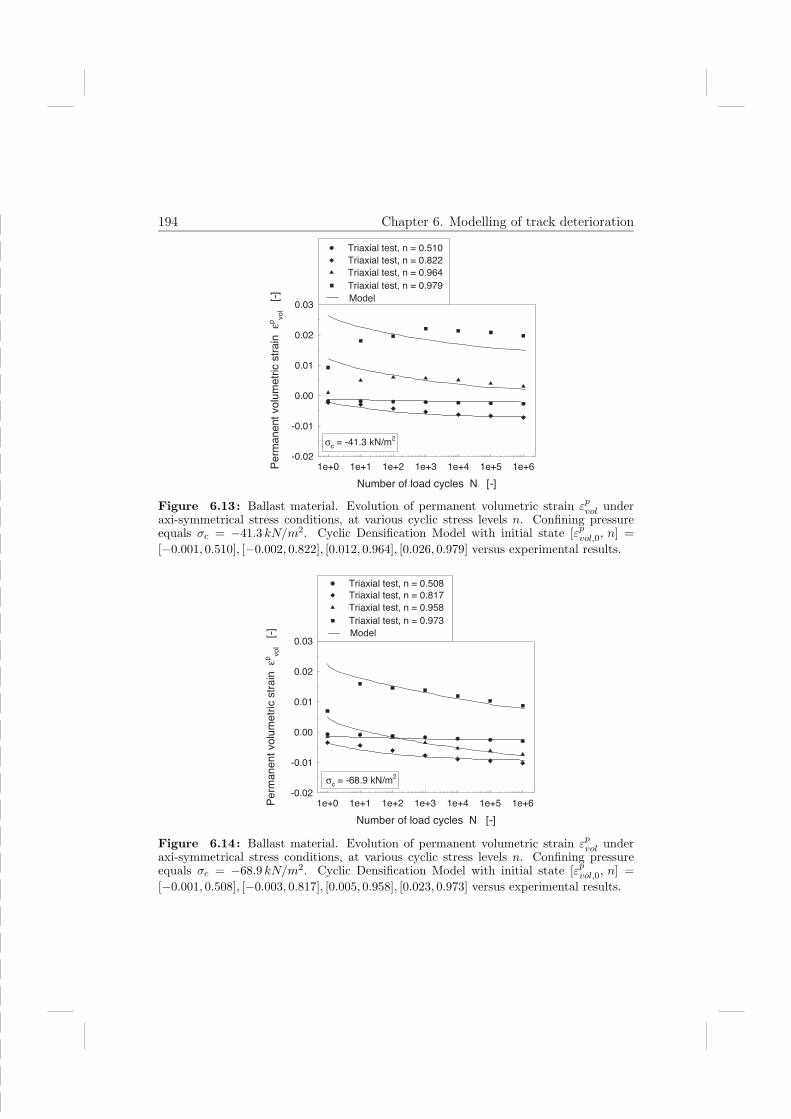
194 Chapter 6. Modelling of track deterioration
Number of load cycles N [-]
1e+0 1e+1 1e+2 1e+3 1e+4 1e+5 1e+6Perm
anent volu
metr
ic s
train
εp
vo
l [
-]
-0.02
-0.01
0.00
0.01
0.02
0.03
Triaxial test, n = 0.510
Triaxial test, n = 0.822
Triaxial test, n = 0.964
Triaxial test, n = 0.979
Model
σc = -41.3 kN/m2
Figure 6.13: Ballast material. Evolution of permanent volumetric strain εpvol under
axi-symmetrical stress conditions, at various cyclic stress levels n. Confining pressureequals σc = −41.3 kN/m2. Cyclic Densification Model with initial state [εp
vol,0, n] =[−0.001, 0.510], [−0.002, 0.822], [0.012, 0.964], [0.026, 0.979] versus experimental results.
Number of load cycles N [-]
1e+0 1e+1 1e+2 1e+3 1e+4 1e+5 1e+6Perm
anent volu
metr
ic s
train
εp
vo
l [
-]
-0.02
-0.01
0.00
0.01
0.02
0.03
Triaxial test, n = 0.973
Triaxial test, n = 0.958
Triaxial test, n = 0.817Triaxial test, n = 0.508
Model
σc = -68.9 kN/m2
Figure 6.14: Ballast material. Evolution of permanent volumetric strain εpvol under
axi-symmetrical stress conditions, at various cyclic stress levels n. Confining pressureequals σc = −68.9 kN/m2. Cyclic Densification Model with initial state [εp
vol,0, n] =[−0.001, 0.508], [−0.003, 0.817], [0.005, 0.958], [0.023, 0.973] versus experimental results.

6.6 Case study 195
Parameters Corresponding equation Subballast Ballast
αf Eq.(6.88-a) 1.0× 10⁻³ [−] 5.0× 10⁻³ [−]γf Eq.(6.88-a) 2.5 [−] 4.0 [−]pt
num Eq.(6.88-a) 10 [kPa] 10 [kPa]αc Eq.(6.88-b) 5.0× 10⁻⁵ [−] 1.0× 10⁻³ [−]γc Eq.(6.88-b) 4.0 [−] 3.0 [−]p0 Eq.(6.88-b) −60 [kPa] −50 [kPa]h0 Eq.(6.37) 0.50 [−] 0.70 [−]hm Eq.(6.37) 1.56 [−] 1.85 [−]ηf Eq.(6.37) 120 [−] 120 [−]ηc Eqs.(6.38) 150 [−] 2000 [−]d0 (= dm) Eq.(6.40) -0.70 [−] -0.50 [−]
Table 6.2 : Calibrated parameters for cyclic plastic model.
material initially reveals a tendency to dilate, the effect of which has not beenincorporated into the Cyclic Densification Model6. However, this discrepancy isless important, because the number of load cycles commonly associated with trackdeterioration lies far beyond one hundred, and for more than one hundred loadcycles the evolution of the permanent volumetric deformation is predicted ratherwell at high stress levels.
6.6 Case study
In this section, the Cyclic Densification Model will be used to study the developmentof permanent deformations in a ballasted railway track under a large number of trainaxle passages. The predictions by a finite element simulation will be compared toin-situ measurements carried out at a railway test-track located at the US/DOTTransportation Center in Pueblo, Colorado (Selig et al., 1981).
6.6.1 Initial state
The initial state of the in-situ ballast and subballast material, which represents thematerial state at the onset of the train loading, is computed by means of an elasto-plastic model for monotonic loading. The parameters of this model are calibratedon the material response obtained from the static triaxial tests in Chapter 5. Thisseems plausible, in a sense that the grain size distribution of the in-situ materials
6For simplicity reasons, both for the subballast and the ballast the evolution law, Eq.(6.40),has been assumed as constant, df (κp) = d0, where d0 has a negative value, see Table 6.2. Thissimplification implies that frictional sliding is always accompanied by volumetric contraction.

196 Chapter 6. Modelling of track deterioration
and the tested materials exhibit a good correspondence, see Figure 5.1. The yieldconditions reflecting frictional sliding and volumetric compaction under monotonicloading are respectively given by
f f (q, p, κp0) = −q/(p− pt
num) − Hf(κp0) = 0 (6.132)
andf c(p, εp
vol,c,0) = p/p0 − Hc(εpvol,c,0) = 0. (6.133)
In accordance with the above expressions, in the principal stress space static failureis described by a Drucker-Prager cone that is limited in the hydrostatic axis by acompression cap. The evolution functions Hf and Hc appearing in Eqs.(6.132) and(6.133) are
Hf (κp0) = H0 + (Hm −H0) (1− exp(−ζfκp
0)) (6.134)
andHc(εp
vol,c,0) = 1 + ζcεpvol,c,0. (6.135)
These expressions have a form comparable to that of the shakedown evolutionfunctions, Eqs.(6.37) and (6.38), depicted in Figures 6.3 and 6.4. The plastic flowdirections corresponding to the frictional sliding criterion, Eq.(6.132), and the volu-metric compaction criterion, Eq.(6.133), are determined in the same manner as forthe cyclic model, see Section 6.3.2. Also, the numerical update procedure for themonotonic elasto-plastic model is similar to that for the cyclic elasto-plastic model,and can be retrieved from the framework presented in Section 6.4.3 by replacing theshakedown evolution functions hf
sh and hcsh in Eqs.(6.98) and (6.105) by the evolu-
tion functions Hf and Hc, respectively, and by representing the history parametercategory, Eq.(6.106), via the two yield conditions, Eqs.(6.132) and (6.133).The parameters characterising the yield functions and the evolution functions
have been quantified in Table 6.3. A reasonable agreement with the static triaxialtest results presented in Sections 5.1.1 and 5.2.2 is obtained, as can be seen fromFigures 6.15 and 6.16 for a confining pressure σc = −68.9 kN/m2. The predictionof the elastic behaviour, represented by the initial part of the curves, appears tobe somewhat too stiff, which is due to the fact that the elastic model has beencalibrated on the material response obtained after the application of 100 load cycles(see Table 6.1).
6.6.2 Update at tensile failure regime
Due to the ’bending capacity’ of the ballast layer, the train loading may causestress points at the surface of the ballast layer to tend towards the tensile failureregime depicted in Figure 6.2. This may induce some problems, because the stressratio −q/p in Eqs.(6.32) and (6.34) will go to infinity when the hydrostatic stress

6.6 Case study 197
Deviatoric strain κ [-]
0.00 0.02 0.04 0.06 0.08 0.10
Str
ess r
atio -q
/ p [
-]
0.0
0.5
1.0
1.5
2.0
2.5
3.0
Subballast
Ballast
Triaxial test, σc= -68.9 kN/m2
Model
Figure 6.15: Stress-strain response of subballast and ballast material under static,axi-symmetrical stress conditions. Experiment versus model. Confining pressure equalsσc = −68.9 kN/m2.
Deviatoric strain κ [-]
0.00 0.01 0.02 0.03 0.04 0.05
Vo
lum
etr
ic s
tra
in
ε vo
l [
-]
-0.02
-0.01
0.00
0.01
0.02
0.03
0.04
0.05
Ballast
Subballast
Triaxial test, σc= -68.9 kN/m2
Model
Figure 6.16: Deformations characteristics of subballast and ballast material understatic, under axi-symmetrical stress conditions. Experiment versus model. Confiningpressure equals σc = −68.9 kN/m2.

198 Chapter 6. Modelling of track deterioration
Parameters Corresponding equation Subballast Ballast
ptnum Eq.(6.132) 10 [kPa] 10 [kPa]
p0 Eq.(6.133) −60 [kPa] −60 [kPa]H0 Eq.(6.134) 0.80 [−] 1.0 [−]Hm Eq.(6.134) 1.56 [−] 1.85 [−]d0 Eq.(6.40) 0.20 [−] 0.20 [−]dm Eq.(6.40) 1.0 [−] 1.10 [−]ζf Eqs.(6.40) and (6.134) 100 [−] 80 [−]ζc Eqs.(6.135) 80 [−] 250 [−]
Table 6.3: Calibrated parameters for monotonic plastic model representing the initialstate.
becomes zero. Moreover, trial stress states beyond the apex (p, q) = (0, 0) mustbe corrected in an appropriate manner. Therefore, the stress update at the tensilefailure regime is treated as follows. The evolution function describing frictionalsliding is extended with a tensile hydrostatic stress pt
num, see Eq.(6.88-a), turningthe condition for frictional shakedown into
f fsh(q, p, κ
p) =(− q/(p− pt
num))
cyc− hf
sh(κp) = 0. (6.136)
Note that a similar adaptation has been made for frictional failure under monotonicloading, see Eq.(6.132), where in both expressions the value for pt
num is chosenrelatively small, i.e. pt
num = 10 kPa, see Tables 6.2 and 6.3. Subsequently, atension cut-off is formulated, which prevents the occurrence of stress points with ahydrostatic stress larger than pt = 5 kPa. The mathematical form of the tensioncut-off is
f t(p) = p − pt = 0. (6.137)
The nature of the above procedure is visualised in Figure 6.17. The corner pointat which the mechanisms of tensile failure and frictional sliding intersect, can bedealt with by means of Koiter’s generalisation theorem (Koiter, 1953), such thatthe plastic strain per cycle follows from
dεpij
dN=
dκp
dNmf
ij +dεp
vol,t
dNmt
ij. (6.138)
Here, the determination of the magnitude and direction of the frictional slidingmechanism occurs in a similar way as explained in Section 6.3. Furthermore, εp
vol,t
is the volumetric plastic strain due to tensile failure, whose magnitude is prescribed(in an incremental fashion) by Prager’s consistency condition, f t(p) = 0, and mt
ij.

6.6 Case study 199
0
tensile failure
frictional failure
cyclic
κ p) = 0, Eq.(6.132)f f
0(q, p,
densification
shakedown
q
(p) = 0, Eq.(6.137)ft
pnum
pt
t
p
p) = 0, Eq.(6.136)
(-)
fshf (q, p, κ
Figure 6.17 : Transition between the regimes of frictional sliding and tensile failure.
is the (associative) flow direction corresponding to tensile failure,
mtij =
∂f t(p)
∂ p
∂ p
∂ σij
=δij
3. (6.139)
The numerical update procedure for the combination of frictional sliding and tensilefailure is comparable to that presented for the combination of frictional sliding andvolumetric compaction, see Section 6.4.3. Accordingly, in the case of tensile failure,the history parameter∆εp
vol,c in Eq.(6.99) needs to be replaced by∆εpvol,t, Eq.(6.106-
b) needs to be replaced by Eq.(6.137), and the function hcsh appearing in Eqs.(6.98)
and (6.105-b) must be frozen.For reaching a proper convergence for integration points subjected to a combina-
tion of frictional sliding and tensile failure, relatively small incremental integrationsteps are commonly required. In order to maintain a large(r) step size for theother integration points in the modelled system, a sub-stepping algorithm is ap-plied, which, if necessary, performs the incremental update at integration pointlevel by means of a division into sub-increments. The number of sub-increments isgoverned by a recursive bisection procedure, where, in the case the iterative pro-cess fails, the actual (strain) increment is bisected into two sub-increments thatprovide the input for a renewed update process. If no convergence is found for a

200 Chapter 6. Modelling of track deterioration
specific sub-increment, the update process is recommenced at the end of the lastconverged (sub-)increment, thereby employing a smaller incremental step size thatyields from bisecting the sub-increment currently failing. The bisection process iscontinued until the size of the sub-increment is small enough to provide a convergedsolution.
6.6.3 Modelling aspects and results
In the case study, the dynamic effect of a moving axle load on the track is thoughtto be represented by a quasi-static line load. The amplitude of the line load in thelongitudinal track direction is set to correspond to the envelope of the (varying)dynamic amplitude of the moving axle load. The track settlement simulation maybe conceived as a pseudo plane strain problem if the variation in load amplitudeinitiated by structural inhomogeneities in the longitudinal direction of the track isnegligible. In other words, the plane strain assumption, which in this case studyis considered to be valid, corresponds to a railway track that has (approximately)homogeneous geometrical and material characteristics in the direction of axle loadpropagation.The dimensions and the mesh of the finite element model employed are depicted
in Figure 6.18. For symmetry reasons, only half of the Colorado test-track is sim-ulated. Roller boundary conditions are imposed to warrant this symmetry, andto prevent rigid body motion. The mesh is constructed by 3312 plane strain,three-node iso-parametric elements, forming cross-diagonal patches. The trian-gular elements use a 1-point Gauss integration scheme, which corresponds to aconstant strain description. As demonstrated by Groen (1997), for boundary valueproblems concerning dilatant/contractant plastic flow, cross-diagonal patches ofthree-noded constant strain triangles are preferable in order to avoid problems oflocking and spurious element behaviour. The mesh is constructed of various ele-ment sizes, where the displacement compatibility at interfaces between elements ofdifferent size is warranted by means of tyings. The representative loading, gener-ated by the train and exerted on the sleeper via the rail fastening system, equalsprail = 1460 kN/m1. This value follows from the fact that the average wheel loadof the train used in the test-track equals 146 kN (Selig et al., 1981), and the effec-tive width of the rail fastening system is estimated as 0.1m. As stated before, theloading process is separated into two stages; a monotonic loading stage and a cyclicloading stage. The monotonic loading stage consists of the application of the deadweight loading, followed by the application of the train wheel loading. The state ofdeformation resulting from the monotonic loading stage represents the initial statefor the subsequent cyclic loading stage.The plastic material parameters for the ballast and subballast are given in Ta-
ble 6.2 (cyclic loading stage) and in Table 6.3 (monotonic loading stage). The

6.6 Case study 201
152
rail
subgrade
788
381
4267
150
9600
1350
2400
rail = 1460 kN/m1p
4800
1800
Plane of symmetry
sleeper
subballastballast
]mmAll measures in [
Figure 6.18: Dimensions and finite element configuration of track model. The fi-nite element configuration is constructed by 3312 plane strain three-node iso-parametricelements with a 1-point Gauss integration scheme.

202 Chapter 6. Modelling of track deterioration
elastic material parameters for both loading stages are presented in Table 6.1. Be-cause for the subgrade material no test data are available, two illustrative caseswill be analysed, which are : case 1, in which the first 1067 mm of subgrade ma-terial situated below the subballast layer is given the same elasto-plastic materialproperties as the subballast while the remaining subgrade material is simulated ashypo-elastic, and case 2, where all subgrade material is simulated as hypo-elastic.The hypo-elastic material behaviour of the subgrade occurs in accordance with thesame elastic material parameters as those of the subballast, see Table 6.1. Case 1will be designated as ’FEM model with elasto-plastic subgrade’ and case 2 will bedesignated as ’FEM model with elastic subgrade’. Furthermore, the wooden sleepersare modelled as linear elastic, with a Young’s modulus equal to E = 10000MPaand a Poisson’s ratio of ν = 0.3. The densities used in the dead weight calculationare ρ = 800 kg/m3 (sleepers), ρ = 1650 kg/m3 (ballast), and ρ = 1920 kg/m3 (sub-ballast and subgrade). Here, the densities of the ballast and subballast materialcorrespond to the values that were experimentally determined, see Table 5.2 andTable 5.5.As described above, in the present model the mechanical effect exerted by a
moving axle load on the track is simulated by means of a quasi-static line load.However, care should be taken regarding the overestimation of stress that goeswith a line load representation. The overestimation of stress is due to the fact thatstress attenuation in the longitudinal direction of the track, which is characteristicfor a point load signature, remains absent for a line load signature. Consequently,the track deformation and track stiffness in a plane strain analysis will be overpre-dicted if no special precautions are taken. In order to compensate for this effect,the stiffness parameters Kref , and the stress parameter pref in Table 6.1, as wellas the stress parameter p0 in Table 6.2 and Table 6.3 are multiplied by correctionfactors. The stress parameter pt
num does not need to be corrected, since this is an’artificial’ parameter. The correction factors stem from a FEM model in which thestress distribution σzz in the longitudinal track direction is computed, as generatedby the dead weight loading and the surface loading psl., see Figure 6.19. Here, thesurface loading has a value that is representative for the stress level directly belowthe sleeper; psl. = 1000 kPa. Furthermore, the ballast, subballast and subgradematerial are modelled in this computation as hypo-elastic, with the material pa-rameters given in Table 6.1 (the subgrade has the same material characteristics asthe subballast).

6.6 Case study 203
sl.
19250
sleeperp
z
All measures in [
15
2
46
48
x0
]mm
zz
/ 5.43sl.-p
-p
-p
-p
=
sl.
sl.
sl.
/ 1.26
/ 2.18
/ 3.22
=
σzz
(z=286 mm)σ
250
38
1
(z=457 mm)
=
=
=(z=913 mm)zzσ
Stress profile at x=0
subgrade
subballast
ballast
zz
sl.-p(z=0 mm)σ
zz
(z=95 mm)σ
Figure 6.19: Model for determination of the stress distribution in the longitudinaldirection of the track. Due to symmetry, only the right half (x ≥ 0) of the sketched con-figuration has been modelled, using 9240 plane strain three-node iso-parametric elementswith a 1-point Gauss integration point scheme. The depicted stress profile σzz occurs be-neath the sleeper at x = 0, as a result of a representative sleeper loading psl. (= 1000 kPa)and the dead weight loading.
As can be seen from Figure 6.19, the correction factors for the ballast are 1.26 (upperpart ballast layer) and 2.18 (lower part ballast layer), while for the subballast layerand the subgrade the correction factors are 3.22 and 5.437, respectively.Figures 6.20 and 6.21 exhibit the cyclic evolution of the vertical permanent strain,
εpzz, in the ballast layer and the subballast layer, respectively, as recorded beneaththe rail and averaged over the corresponding layer thickness. The in-situ ballaststrain measurements were taken both beneath the inside rail and beneath the out-side rail of the track, at four different sleeper positions; 20E − 0901, 20E − 0909,20E − 0917, and 20E − 0935. For the subballast layer, the in-situ strain measure-ments were taken also beneath both rails, though at two different sleeper positions;20E−0909 and 20E−0917. The indication ’20E’ thereby refers to the track sectionwith traprock ballast and wooden sleepers (Selig et al., 1981). In the figures, theevolution of the permanent strain is characterised by means of load cycles, wherethe in-situ data has been converted by using the fact that three train axle pas-sages correspond to one load cycle. This ratio has been deduced from the dynamicresponse recorded during an instantaneous train passage (Selig et al., 1981). As
7The use of a single correction factor for the complete subgrade is a somewhat crude approxima-tion, most likely causing the deformations in the lower part of the subgrade to be overestimated.Nevertheless, in the current study the subgrade deformation behaviour is considered only in aqualitative way, where the exact determination of the stress attenuation with increasing subgradedepth is of minor importance.

204 Chapter 6. Modelling of track deterioration
Test-track FEM model, FEM model,elasto-plastic subgrade elastic subgrade
Reversible strain ballast layer -0.0049 [−] -0.0021 [−] -0.0023 [−]Reversible strain subballast layer -0.0015 [−] -0.0021 [−] -0.0021 [−]
Table 6.4: Reversible vertical strain εezz beneath the rail, recorded after the application
of 30480 load cycles. The strain measurements for the Colorado test-track have beenreproduced from Selig et al. (1981).
illustrated by Figures 6.20 and 6.21, the strains computed at the end of the cyclicloading process are in the same range as the corresponding strain values obtainedfrom the in-situ measurements. It can be observed that the in-situ measurementsreveal a significant scatter, probably caused by the non-uniform structural proper-ties in the longitudinal track direction. In the FEM model, shakedown is reachedfaster than in the test-track, which is especially true for the ballast layer. Also,in both the FEM model and the test-track, the vertical permanent deformation ofthe subballast layer is consistently larger than that of the ballast layer. Similarconclusions can be drawn from the cyclic strain evolution recorded beneath thesleeper centre, see Figure 6.22 (ballast layer) and Figure 6.23 (subballast layer).Comparing Figures 6.22 and 6.23 with Figures 6.20 and 6.21 reveals that the
deformations beneath the rail generally are larger than the deformations beneaththe sleeper centre. This can also be observed from Figure 6.24, which sketchesthe deformation pattern computed after the application of N = 60000 load cycles.Apparently, the elasto-plastic subgrade model results in a maximum displacementbelow the load that is nearly twice as large as that for the elastic subgrade model.Despite of this significant discrepancy, the effect of different subgrade character-istics on the permanent strain development in the ballast and subballast is onlymarginal, see Figures 6.20 to 6.23.Table 6.4 presents the reversible vertical strain, εe
zz, in the ballast and subballastlayer, recorded beneath the rail during an individual train axle passage, after theapplication of 30480 load cycles. The values for the test-track reflect the averageof 4 measurements. It can be noted that the computed reversible strains are nearlyidentical for both subgrade conditions. Comparing the model results with the mea-sured data illustrates that the reversible strain in the subballast layer is predictedrather well by the model, and that the reversible strain in the ballast layer is un-derestimated by approximately a factor of two. Regarding the latter difference, itneeds to be mentioned that the measured reversible ballast strains providing theaverage ballast strain reveal a considerable variation, in a sense that they rangefrom εe
zz = −0.0015 to εezz = −0.0091 (Selig et al., 1981).
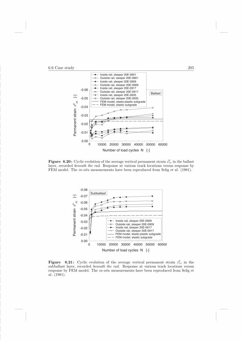
6.6 Case study 205
Number of load cycles N [-]
10000 20000 30000 40000 50000 60000
Perm
anent str
ain
εp
zz
[ -
]
-0.06
-0.05
-0.04
-0.03
-0.02
-0.01
0.00
Ballast
0
Inside rail, sleeper 20E-0901 Outside rail, sleeper 20E-0901
Inside rail, sleeper 20E-0909Outside rail, sleeper 20E-0909Inside rail, sleeper 20E-0917
Outside rail, sleeper 20E-0917Inside rail, sleeper 20E-0935Outside rail, sleeper 20E-0935
FEM model, elastic subgrade FEM model, elasto-plastic subgrade
Figure 6.20: Cyclic evolution of the average vertical permanent strain εpzz in the ballast
layer, recorded beneath the rail. Response at various track locations versus response byFEM model. The in-situ measurements have been reproduced from Selig et al. (1981).
Number of load cycles N [-]
0 10000 20000 30000 40000 50000 60000
Perm
anent str
ain
εp
zz
[ -
]
-0.08
-0.07
-0.06
-0.05
-0.04
-0.03
-0.02
-0.01
0.00
Subballast
FEM model, elastic subgrade
Inside rail, sleeper 20E-0909Outside rail, sleeper 20E-0909Inside rail, sleeper 20E-0917Outside rail, sleeper 20E-0917FEM model, elasto-plastic subgrade
Figure 6.21: Cyclic evolution of the average vertical permanent strain εpzz in the
subballast layer, recorded beneath the rail. Response at various track locations versusresponse by FEM model. The in-situ measurements have been reproduced from Selig etal. (1981).

206 Chapter 6. Modelling of track deterioration
Number of load cycles N [-]
0 10000 20000 30000 40000 50000 60000
Perm
anent str
ain
εp
zz
[ -
]-0.06
-0.05
-0.04
-0.03
-0.02
-0.01
0.00
BallastCentre of sleeper 20E-0909
Centre of sleeper 20E-0917
FEM model, elastic subgradeFEM model, elasto-plastic subgrade
Figure 6.22: Cyclic evolution of the average vertical permanent strain εpzz in the
ballast layer, recorded beneath the sleeper centre. Response at various track locationsversus response by FEM model. The in-situ measurements have been reproduced fromSelig et al. (1981).
Number of load cycles N [-]
0 10000 20000 30000 40000 50000 60000
Perm
anent str
ain
εp
zz
[ -
]
-0.08
-0.07
-0.06
-0.05
-0.04
-0.03
-0.02
-0.01
0.00
Centre of sleeper 20E-0909Centre of sleeper 20E-0917
FEM model, elastic subgradeFEM model, elasto-plastic subgrade
Subballast
Figure 6.23: Cyclic evolution of the average vertical permanent strain εpzz in the
subballast layer, recorded beneath the sleeper centre. Response at various track locationsversus response by FEM model. The in-situ measurements have been reproduced fromSelig et al. (1981).

6.7 Discussion 207
1p = 1460 kN/m
Subgrade behaves elasto-plastically
rail
p = 1460 kN/mrail
Subgrade behaves elastically
1
Figure 6.24: Deformation pattern (magnification factor is 10) for upper part of finiteelement configuration after the application of N=60000 load cycles.
6.7 Discussion
Efficient modelling of track deterioration can be realised by means of an elasto-plastic model that is based upon a description of the permanent strain envelope ofthe cyclic response, instead of on a description of the complete cyclic response. Inaccordance with this concept, a Cyclic Densification Model has been proposed thatcaptures the deformation evolution of a granular material generated by frictionalsliding and volumetric compaction. The theoretical framework of the model hasbeen derived by using the classical plasticity theory as a point of departure. As

208 Chapter 6. Modelling of track deterioration
demonstrated, the model distinguishes between four response regimes, which are (i)shakedown, (ii) cyclic densification, (iii) frictional failure, and (iv) tensile failure.The actual response depends on the applied stress level, the applied stress path,and on the duration of the cyclic loading.
The numerical integration of the Cyclic Densification Model has been based onan implicit Euler backward algorithm with a non-linear elastic stress predictor.The model has been calibrated on test data obtained from triaxial experiments,see Chapter 5. Subsequently, the model has been employed in a finite elementanalysis of track deterioration. For this purpose, the test-track located at theUS/DOT Transportation Center in Pueblo, Colorado has been modelled, whichwas previously submitted to an extensive measuring program in order to assess itslong-term settlement behaviour due to repetitive train loading (Selig et al., 1981).The data that yielded from these in-situ measurements has been compared to theresults of the finite element analysis.
The measured deformation level corresponding to shakedown was predicted rea-sonably well by the FEM model. However, in the FEM model shakedown wasreached considerably faster than in the test-track. The differences between thetest-track response and the response of the FEM model are believed to be due tovarious factors.
Firstly, the densities of the materials tested in the laboratory (see Chapter 5)may not be exactly correspondent to those of the in-situ materials. The difficulty ofsimulating the appropriate in-situ initial state of a geo-technical structure is a well-known problem in soil mechanics, commonly regarded as one of the main causes forthe discrepancies emerging between model predictions and in-situ measurements.
Secondly, the triaxial experiments that form the basis for the model calibrationdo not always adequately represent the in-situ stress and deformation states. Forexample, a conventional triaxial test can not correctly simulate the train-inducedreversal of shear stress in the longitudinal track direction, which occurs as soonas a material point in the track is located directly below the passing train axle.Disregarding the effect of the shear stress reversal in a laboratory experiment nat-urally yields a different cyclic evolution of the permanent material deformations.Furthermore, the constant geo-static stresses in a railway track are represented inthe triaxial tests by means of a constant confining pressure. This is not correct, ina sense that geo-static stresses do not have a purely hydrostatic nature. Addition-ally, the deviation of the intermediate shear stress with respect to the maximumshear stress is not measured in a conventional triaxial test, see also Section 6.3.1.Moreover, the range of stress levels in the Colorado test-track is not fully coveredby the stress levels applied in the cyclic triaxial experiments, so that in the FEMsimulations on track deterioration the model occasionally is submitted to stresslevels that lie beyond the stress range considered for the model calibration.

6.7 Discussion 209
Thirdly, the simplifications adopted in the modelling procedure may induce dif-ferences between the FEM response and the test-track response. In the Cyclic Den-sification model no explicit distinction can be made between stress contributionsdue to static loading and stress contributions due to cyclic loading. Typically, thecyclic evolution of deformation is considered to be governed by the total of all stresscontributions, which may be somewhat unrealistic for material points subjected toa static stress that is relatively large compared to the cyclic stress contribution.In this respect, it is also important to realise that in boundary value problems theCyclic Densification Model should be activated only for material points that suffera significant cyclic stress contribution (i.e. the material points in the upper part ofa railway track).
In addition, by representing the effect of a moving axle load by a quasi-staticline load, the influence of the previously mentioned shear stress reversal on thecyclic response is omitted. Accordingly, the model can possibly be improved byreplacing the quasi-static line load representing the train loading by a set of staticpoint loads at a given intermediate distance, thus causing shear stresses to emergein the longitudinal track direction. Trivially, only the deformations beneath thestatic point loads should be considered in such a model, since the deformation pro-file arising in between the point loads is unrealistic for a railway track. In fact,the deformation profile in between the point loads should be determined from thedeformations beneath the point loads by means of interpolation techniques. Themagnitude of the (static) shear stress in the longitudinal track direction needs tofurnish the net permanent deformation corresponding to a complete shear stressreversal. Typically, the stress path relating to the complete shear stress reversalis characterised as ’non-proportional’, since the principal stress directions in a ma-terial point change as soon as the shear stress reversal takes place. Nonetheless,the Cyclic Densification Model only describes the net deformation generated bythe stress reversal, such that the actual evolution parameter ’time’ in the modelcan be replaced by the artificial evolution parameter ’load cycle’. By simulatingthe deformation evolution by means of load cycles, non-proportional stress pathsoccurring within a load cycle might be effectively treated as being ’proportional’over a load cycle.
Finally, it is noted that the subgrade material behaviour has been modelled inan approximate manner, by giving it the same elasto(-plastic) material propertiesas the subballast material. This premise appeared to be necessary, since for thesubgrade material no test data were available. Although using more realistic ma-terial parameters for the subgrade is unlikely to significantly alter the ballast andsubballast response currently presented, for the accurate simulation of the overalltrack behaviour such a modification is certainly necessary.
The track model proposed in this chapter is two-dimensional, representing a

210 Chapter 6. Modelling of track deterioration
railway track that is homogeneous in the longitudinal direction. For the simu-lation of differential settlements, induced by inhomogeneities present in the lon-gitudinal track direction, a three-dimensional track model is required. Togetherwith the issues addressed above, the extension of the current approach towardsthree-dimensional modelling of track deterioration leaves sufficient room for fur-ther research. To date, only a very few combined numerical/experimental studieson track deterioration have been reported in the literature, and it is hoped that thepresent study will stimulate more investigations in this direction. The methodologyproposed in this chapter may serve as an appropriate tool for such investigations.

ReferencesAchenbach, J.D. and Sun, J.T. (1965). Moving load on a flexibly supported Tim-oshenko beam. Int. J. Solids Struct. 1, pp. 353–370.
Achenbach, J.D. (1973). Wave propagation in Elastic Solids. Elsevier SciencePublishers b.v. Amsterdam.
Aifantis, E.C. (1992). On the role of gradients in the localization of deformationand fracture. Int. J. Eng. Sci. 30, pp. 1279–1299.
Alva-Hurtado, J.E.D. (1980). A Methodology to Predict the Elastic and Inelas-tic Behaviour of Railroad Ballast. Dissertation, University of Massachusetts,Amherst, Massachusetts, U.S.A.
Anderson, W.F. and Key, A.J. (2000). Model testing of two-layer railway trackballast. J. Geotech. Geoenvironm. Engng. 126(4), pp. 317–323.
AREA. (1988). Manual for Railway Engineering. Section 2.4.4, Gradations.
ASTM D2487. (1997). Standard test method for classification of soils for engi-neering purposes. In Annual Book of ASTM Standards. Section 4, Construction,Volume 04.08, Soil and Rock.
ASTM D698. (1997). Test method for laboratory compaction characteristics ofsoil using standard effort (12.300 ft-lb/ft3 (600 kN-m/m3)). In Annual Book ofASTM Standards. Section 4, Construction, Volume 04.08, Soil and Rock.
Bathe, K.J. (1982). Finite Element Procedures in Engineering Analysis. Prentice-Hall Inc. Englewood Cliffs, New Jersey.
Bathurst, R.J. and Rothenburg, L. (1988). Micromechanical aspects of isotropicgranular assemblies with linear contact interactions. J. Appl. Mech. (ASME) 55,pp. 17–23.
Bazant, Z.P. and Pijaudier-Cabot, G. (1988). Nonlocal continuum damage local-ization, instability and convergence. J. Appl. Mech. (ASME) 55, pp. 287–293.
Bezuijen, A., Molenkamp, F., and van der Kogel, H. (1982). The determination ofparameters for a double hardening model by means of undrained torsional simpleshear tests. In Vermeer, P.A. and Luger, H.J., eds., Deformation and Failure ofGranular Materials, pp. 181–189. A.A. Balkema, Rotterdam.
Borja, R. (1991). Cam-clay plasticity, Part II, Implicit integration of constitutiveequations based on a nonlinear elastic stress predictor. Comp. Meth. Appl. Mech.Engng. 88, pp. 225–240.

212 References
Born, M. and Huang, K. (1954). Dynamical Theory of Crystal Lattices. ClarendonPress, Oxford.
Brillouin, L. (1946). Wave Propagation in Periodic Structures. Dover Publications,Inc. New York.
Brown, S.F. (1974). Repeated load testing of a granular material. J. Geotech.Engng. Div. (ASCE) 100, pp. 825–841.
Cambou, B., Dubujet, P., Emeriault, F., and Sidoroff, F. (1995). Homogenizationfor granular materials. Eur. J. Mech. A/Solids 14, pp. 255–276.
Chambon, R., Caillerie, D., and Matsuchima, T. (2001). Plastic continuum withmicrostructure, local second gradient theories for geomaterials: localization stud-ies. Int. J. Solids Struct. 38, pp. 8503–8527.
Chang, C.S. and Gao, J. (1995). Second-gradient constitutive theory for granularmaterials with random packing structure. Int. J. Solids Struct. 32, pp. 2279–2293.
Chang, C.S. and Gao, J. (1996). Kinematic and static hypotheses for constitutivemodelling of granulates considering particle rotation. Acta Mech. 115, pp. 213–229.
Chang, C.S. and Gao, J. (1997). Wave propagation in granular rod using high-gradient theory. J. Eng. Mech. 123, pp. 52–59.
Chang, C.S. and Liao, C.L. (1990). Constitutive relation for a particulate mediumwith the effect of particle rotation. Int. J. Solids Struct. 26, pp. 437–453.
Chang, C.S. and Ma, L. (1992). Elastic material constants for isotropic granularsolids with particle rotation. Int. J. Solids Struct. 29, pp. 1001–1018.
Chang, C.S. (1988). Micromechanical modelling of constitutive relations for granu-lar material. In Satake, M. and Jenkins, J.T., eds., Micromechanics of GranularMaterial. Elsevier, Amsterdam. pp. 271–279.
Chang, C.S. (1993). Micromechanical modeling of deformation and failure forgranulates with frictional contacts. Mech. Mat. 16, pp. 13–24.
Christofferson, J., Mehrabadi, M.M., and Nemat-Nassar, S. (1981). A microme-chanical description on granular material behavior. J. Appl. Mech. (ASME) 48,pp. 339–344.

References 213
de Borst, R. and Feenstra, P.H. (1990). Studies in anisotropic plasticity withreference to the Hill criterion. Int. J. Num. Meth. Engng. 29, pp. 315–336.
de Borst, R. and Muhlhaus, H.-B. (1992). Gradient-dependent plasticity : Formu-lation and algorithmic aspects. Int. J. Num. Meth. Eng. 35, pp. 521–539.
de Borst, R. and Sluys, L.J. (1991). Localisation in a Cosserat continuum understatic and dynamic loading conditions. Comp. Meth. Appl. Mech. Engng. 90, pp.805–827.
de Borst, R. (1991). Simulation of strain localisation: A reappraisal of the Cosseratcontinuum. Eng. Comp. 8, pp. 317–332.
Deresiewicz, H. (1958). Stress-strain relations for a simple model of a granularmedium. J. Appl. Mech. (ASME) 25, pp. 402–406.
Desai, C.S. and Zhang, D. (1987). Viscoplastic models for geologic materials withgeneralized flow rule. Int. J. Num. Meth. Engng. 11, pp. 603–620.
Dieterman, H.A. and Metrikine, A. (1997a). Critical velocities of a harmonic loadmoving uniformly along an elastic layer. J. Appl. Mech. (ASME) 64, pp. 596–600.
Dieterman, H.A. and Metrikine, A. (1997b). Steady-state displacements of a beamon an elastic half-space due to a uniformly moving constant load. Eur. J. Mech.A/Solids 16, pp. 295–306.
Digby, P.J. (1981). The effective elastic moduli of porous granular rock. J. Appl.Mech. (ASME) 48, pp. 803–808.
Dorr, J. (1943). Der unendliche, federende gebettete Balken unter dem Einflusseiner gleichformig bewegente Last. Ing. Arch. 14, pp. 167–192. (in German).
Duffy, J. and Mindlin, R.D. (1957). Stress-strain relations and vibrations of granularmedium. J. Appl. Mech. (ASME) 24, pp. 585–593.
Eringen, A.C. (1968). Theory of micro-polar elasticity. In Liebowitz, H., ed.,Fracture - An Advanced Treatise, volume II. Academic Press, New York andLondon. chapter 7, pp. 621–693.
Esveld, C. (1989). Modern Railway Track. MRT-Productions, Germany.
Esveld, C. (2001). A cost-effective rail infrastructure. Eur. Railway Rev. 7(2), pp.67–71.
214 References
Ewing, M.E., Jardetzky, W.S., and Press, F. (1957). Elastic Waves in LayeredMedia. McGraw-Hill book company, Inc. New York.
Fillipov, A.P. (1961). Steady state vibrations of an infinite beam on an elastic halfspace subjected to a moving load. Izvestija Akademii Nauk SSSR Mehanika IMashinostroenie 6, pp. 97–105. (in Russian).
Fleck, N.A. and Hutchinson, J.W. (1997). Strain gradient plasticity. Adv. Appl.Mech. 33, pp. 295–361.
Fortin, J-P. (1982). La deformee dynamique de la voie ferree. Revue Generale deChemins de Fer 101, pp. 93–102. (in French).
Fryba, L.J. (1972). Vibration of Solids and Structures under Moving Loads. No-ordhoff International Publishing, Groningen.
Galjaard, P.J., Paute, J.L., and Dawson, A.R. (1996). Comparison and perfor-mance of repeated load triaxial test equipment for unbound granular materi-als. In Gomes Correia, A., ed., Flexible Pavements. A.A. Balkema, Rotter-dam/Brookfield.
Geers, M.G.D. (1997). Experimental Analysis and Computational Modelling ofDamage and Fracture. Dissertation, Eindhoven University of Technology, Eind-hoven, The Netherlands.
Goldscheider, M. (1976). Grenzbedingung und Fliessregel von Sand. Mech. Res.Comm. 3, pp. 463–468. (in German).
Grassie, S.L. (1995). Dynamic modelling of concrete railway sleepers. J. SoundVibr. 187, pp. 799–813.
Groen, A.E. (1995). Elastoplastic modelling of sand using a conventional model. I.Theory and numerical implementation. Technical Report 03.21.0.31.34, Depart-ment of Civil Engineering, Delft University of Technology, Delft, The Nether-lands.
Groen, A.E. (1997). Three-dimensional Elasto-plastic Analysis of Soils. Disserta-tion, Delft University of Technology, Delft, The Netherlands.
Heeres, O.M., Suiker, A.S.J., and de Borst, R. (2002). A comparison betweenthe Perzyna viscoplastic model and the Consistency viscoplastic model. Eur. J.Mech. A/Solids 21, pp. 1–12.

References 215
Hill, R. (1957). On uniqueness and stability in the theory of finite elastic strain.J. Mech. Phys. Solids 5, pp. 229–241.
Hjortnaes-Pedersen, A. and Molenkamp, F. (1982). Accuracy and reproducibilityof triaxial tests. In Vermeer, P.A. and Luger, H.J., eds., Deformation and Failureof Granular Materials, pp. 391–401. A.A. Balkema, Rotterdam.
Hughes, T.J.R. (1987). The Finite Element Method, Linear Static and DynamicFinite Element Analysis. Prentice-Hall International, Inc., New Jersey.
Hunt, G.A. (1994). Analysis of requirements for railway construction on softground. Technical Report LR TM 031, British Rail Research, London, England.
Indraratna, B, Ionescu, D., and Christie, H.D. (1998). Smear behavior of ballastbased on large-scale triaxial tests. J. Geotech. Geoenvironm. Engng. 124(5), pp.439–449.
Jenkins, J.T. (1988). Volume change in small strain axisymmetric deformationsof granular material. In Satake, M. and Jenkins, J.T., eds., Micromechanics ofGranular Materials. Elsevier, Amsterdam. pp. 143–152.
Kaynia, A.M., Madshus, C., and Zackrisson, P. (2000). Ground vibration fromhigh-speed trains: prediction and countermeasure. J. Geotech. Geoenvironm.Engng. 126, pp. 531–537.
Kjorling, M. (1993). Measurements on the track at Algaras, between Laxa andToreboda, Sweden. TRITA-BST-0161, Royal Institute of Technology, Stockholm,Sweden.
Knothe, K. and Grassie, S.L. (1993). Modelling of railway track and of vehicle/trackinteraction at high frequencies high frequencies. Veh. Syst. Dyn. 22, pp. 209–262.
Koiter, W.T. (1953). Stress-strain relations, uniqueness and variational theoremsfor elasto-plastic materials with a singular yield surface. Q. Appl. Mech. 11, pp.350–354.
Kolsky, H. (1963). Stress Waves in Solids. Dover Publications, Inc. New York.
Kononov, A.V. and Wolfert, A.M. (2000). Load motion along a beam on a vis-coelastic half space. Eur. J. Mech. A/Solids 19, pp. 361–371.
Korn, G.A. and Korn, T.M. (1961). Mathematical Handbook for Scientists andEngineers. McGraw-Hill, New York.

216 References
Kunin, I.A. (1982). Elastic Media with Microstructure - Vol 1 - One-dimensionalmodels. Springer-Verlag, Berlin.
Kunin, I.A. (1983). Elastic Media with Microstructure, Vol. 2, Three-dimensionalModels. Springer-Verlag, Berlin.
Labra, J.J. (1975). An axially stressed railroad track on an elastic continuumsubjected to a moving load. Acta Mech. 22, pp. 113–129.
Lade, P.V. and Kim, M.K. (1988). Single hardening constitutive model for frictionalmaterials: III. Comparison with experimental data. Comput. Geotech. 6, pp. 31–47.
Lade, P.V. (1977). Elasto-plastic stress-strain theory for cohesionless soil withcurved yield surfaces. Int. J. Solids Struct. 13, pp. 1019–1035.
Lade, P.V. (1982). Localization effects in triaxial tests on sand. In Vermeer,P.A. and Luger, H.J., eds., Deformation and Failure of Granular Materials, pp.461–471. A.A. Balkema, Rotterdam.
Lago, T.L., Hermodsson, M., Persson, P., and Sjosten, P. (1998). Active vibrationreduction in a light high-speed train bogie. In Proceedings of the 16th Inter-national Modal Analysis Conference. Santa Barbara, California. pp. volume 1,240–246.
Landau, L.D. and Lifshitz, E.M. (1976). Mechanics. Pergamon, Oxford.
Lansing, D.L. (1966). The displacements in an elastic half-space due to a movingconcentrated normal load. Nasa technical report, TR R-238, Langley ResearchCenter, Langley station, Hampton, Va.
Lemaitre, J. and Chaboche, J.-L. (1990). Mechanics of Solid Materials. CambridgeUniversity Press, Cambridge.
Liao, C.L., Chang, T.P., Young, D.H., and Chang, C.S. (1997). Stress-strainrelationships for granular materials based on the hypothesis of best-fit. Int. J.Solids Struct. 34, pp. 4087–4100.
Liao, C.L., Chan, T.C., Suiker, A.S.J., and Chang, C.S. (2000). Pressure-dependentelastic moduli of granular assemblies. Int. J. Num. Anal. Meth. Geomech. 24,pp. 265–279.
Lieb, M. and Sudret, B. (1998). A fast algorithm for soil dynamics calculations bywavelet decomposition. Arch. Appl. Mech. 68, pp. 147–157.

References 217
Luenberger, D.G. (1984). Introduction to Linear and Nonlinear Programming.Addison-Wesley.
Madshus, C. and Kaynia, A.M. (2000). High-speed railway lines on soft ground:dynamic behaviour at critical train speed. J. Sound. Vibr. 231, pp. 689–701.
Maradudin, A.A., Montroll, E.M., Weiss, G.H., and Ipatova, I.P. (1971). Theory ofLattice Dynamics in the Harmonic Approximation. Solid State Physics, Suppl.3, Academic, New York.
Metrikine, A.V. and Popp, K. (1999). Vibration of a periodically supported beamon an elastic half-space. Eur. J. Mech. A/Solids 18, pp. 679–701.
Mindlin, R.D. (1964). Micro-structure in linear elasticity. Arch. Ration. Mech.Anal. 16, pp. 51–78.
Mindlin, R.D. (1965). Second gradient of strain and surface-tension in linearelasticity. Int. J. Solids Struct. 1, pp. 417–438.
Muhlhaus, H.-B. and Oka, F. (1996). Dispersion and wave propagation in discreteand continuous models for granular materials. Int. J. Solids Struct. 33, pp.2841–2858.
Muhlhaus, H.-B. and Vardoulakis, I. (1987). The thickness of shear bands ingranular materials. Geotechnique 37, pp. 271–283.
Nordborg, A. (1998). Vertical rail vibrations: Pointforce excitation. Acta Acustica.84, pp. 280–288.
Oda, M., Iwashita, K., and Kazama, H. (1997). Micro-structure developed in shearbands of dense granular soils and its computer simulation -Mechanism of dila-tancy and failure -. In Fleck, N.A. and Cocks, A.C.F., eds., IUTAM Symposiumon Mechanics of Granular and Porous Materials, pp. 353–364. Kluwer AcademicPublishers, Dordrecht, The Netherlands.
Olszak, W. and Perzyna, P. (1969). On thermal effects in viscoplasticity. J. Appl.Math. Phys. 20, pp. 676–680.
Ortiz, M. and Popov, E.P. (1985). Accuracy and stability of integration algorithmsfor elastoplastic constitutive relations. Int. J. Num. Meth. Engng. 21, pp. 1561–1576.
Pamin, J. (1994). Gradient-dependent Plasticity in Numerical Simulation of Lo-calization Phenomena. Dissertation, Delft University of Technology, Delft, TheNetherlands.

218 References
Peerlings, R.H.J., de Borst, R., Brekelmans, W.A.M., and De Vree, J.H.P. (1996).Gradient-enhanced damage for quasi-brittle materials. Int. J. Num. Meth. Eng.39, pp. 3391–3403.
Peerlings, R.H.J., Brekelmans, W.A.M., de Borst, R., and Geers, M.G.D. (2000).Gradient-enhanced damage modelling of high-cycle fatigue. Int. J. Num. Meth.Engng. 49, pp. 1547–1569.
Perzyna, P. (1966). Fundamental problems in viscoplasticity. Rec. Adv. Appl.Mech. 9, pp. 243–377.
Raymond, G.P. and Davies, J.R. (1978). Triaxial tests on dolomite railroad ballast.J. Geotech. Engng. Div. (ASCE) 104, pp. 737–751.
Raymond, G.P. and Williams, D.R. (1978). Repeated load triaxial tests on adolomite ballast. J. Geotech. Engng. Div. (ASCE) 104, pp. 1013–1029.
Ristinmaa, M.R. and Ottosen, N.S. (2000). Consequences of dynamic yield surfacein viscoplasticity. Int. J.Solids Struct. 37, pp. 4601–4622.
Rothenburg, L. and Selvadurai, A.P.S. (1981). Micromechanical definition of theCauchy stress tensor for particulate media. In Selvadurai, A.P.S., ed., Mechanicsof Structured Media. Elsevier, Amsterdam. pp. 469–486.
Runesson, K., Samuelsson, A., and Bernspang, L. (1986). Numerical technique inplasticity including solution advancement control. Int. J. Num. Meth. Engng.22, pp. 119–130.
Selig, E.T. and Waters, J.M. (1994). Track Geotechnology and Substructure Man-agement. Thomas Telford Services Ltd, London.
Selig, E.T., Yoo, T.S., Adegoke, C.W., and Stewart, H.E. (1981). Status report- Ballast experiments, Intermediate (175 mgt), Substructure stress and straindata. Technical Report FAST/TTC/TM-81/03, University of Massachusetts, forU.S. DOT Transportation Systems Center, Cambridge, MA, U.S.A.
Simo, J.C. and Hughes, T.J.R. (1998). Computational Inelasticity. Springer-Verlag,New York.
Simo, J.C. and Taylor, R. L. (1985). Consistent tangent operators for rate-independent elasto-plasticity. Comp. Meth. Appl. Mech. Engng. 48, pp. 101–118.
Simo, J.C. and Taylor, R.L. (1986). A return-mapping algorithm for plane stresselastoplasticity. Int. J. Num. Meth. Engng. 22, pp. 649–670.

References 219
Simo, J.C., Kennedy, J.G., and Govindjee, S. (1988). Non-smooth multisurfaceplasticity and viscoplasticity. Loading/unloading conditions and numerical algo-rithms. Int. J. Num. Meth. Engng. 26, pp. 2161–2185.
Sluys, L.J. (1992). Wave Propagation, Localisation and Dispersion in SofteningSolids. Dissertation, Delft University of Technology, Delft, The Netherlands.
Stewart, H.E. (1982). The Prediction of Track Performance under Dynamic TrafficLoading. Dissertation, University of Massachusetts, Amherst, Massachusetts,U.S.A.
Suiker, A.S.J. and Chang, C.S. (2000). Application of higher-order tensor theoryfor formulating enhanced continuum models. Acta Mech. 142, pp. 223–234.
Suiker, A.S.J. and de Borst, R. (2002). Enhanced continua and discrete lattices formodelling granular assemblies. Phil. Trans. R. Soc. (London) ser. A (acceptedfor publication).
Suiker, A.S.J. and Esveld, C. (1997). Stiffness transition subjected to instanta-neous moving load passage. In Proc. Sixth International Heavy Haul RailwayConference. Capetown, South Africa. pp. 1194–1205.
Suiker, A.S.J., de Borst, R., and Esveld, C. (1998). Critical behaviour of a Timo-shenko beam-half plane system under a moving load. Arch. Appl. Mech. 68, pp.158–168.
Suiker, A.S.J., Chang, C.S., de Borst, R., and Esveld, C. (1999a). Surface waves ina stratified half space with enhanced continuum properties - Part 1 - Formulationof the boundary value problem. Eur. J. Mech. A/Solids 18, pp. 749–768.
Suiker, A.S.J., Chang, C.S., de Borst, R., and Esveld, C. (1999b). Surface wavesin a stratified half space with enhanced continuum properties - Part 2 - Analysisof the wave characteristics in regard to high-speed railway tracks. Eur. J. Mech.A/Solids 18, pp. 769–784.
Suiker, A.S.J., Metrikine, A.V., and de Borst, R. (2000). Steady state response ofa granular layer to a moving load. Heron 45, pp. 75–87.
Suiker, A.S.J., de Borst, R., and Chang, C.S. (2001a). Micro-mechanical mod-elling of granular material - Part 1 - Derivation of a second-gradient micro-polarconstitutive theory. Acta Mech. 149, pp. 161–180.
220 References
Suiker, A.S.J., de Borst, R., and Chang, C.S. (2001b). Micro-mechanical modellingof granular material - Part 2 - Plane wave propagation in infinite media. ActaMech. 149, pp. 181–200.
Suiker, A.S.J., Metrikine, A.V., and de Borst, R. (2001c). Comparison of wavepropagation characteristics of the Cosserat continuum model and correspondingdiscrete lattice models. Int. J. Solids Struct. 38, pp. 1563–1583.
Suiker, A.S.J., Metrikine, A.V., and de Borst, R. (2001d). Dynamic behaviour ofa layer of discrete particles - Part 1 - Analysis of body waves and eigen modes.J. Sound Vibr. 240, pp. 1–18.
Suiker, A.S.J., Metrikine, A.V., and de Borst, R. (2001e). Dynamic behaviour of alayer of discrete particles - Part 2 - Response to a uniformly moving, harmonicallyvibrating load. J. Sound Vibr. 240, pp. 19–39.
Suiker, A.S.J. (1996). Dynamic behaviour of homogeneous and stratified mediaunder pulses and moving loads. Technical Report 7-96-119-1, Department ofCivil Engineering, Delft University of Technology, Delft, The Netherlands.
Suiker, A.S.J. (1998). Fatigue behaviour of granular materials. Part 2: Numericalformulation of the constitutive relations. Technical Report 7-98-119-3, Depart-ment of Civil Engineering, Delft University of Technology, Delft, The Nether-lands.
Suiker, A.S.J. (1999). Static and cyclic loading experiments on non-cohesive gran-ular materials. Technical Report 1-99-DUT-1, Department of Civil Engineering,Delft University of Technology, Delft, The Netherlands.
Tatsuoka, F. and Ishihara, K. (1974). Yielding of sand in triaxial compression.Soils and Found. 14, pp. 63–76.
TGV-web. (2000). Internet web-site. http : //mercurio.iet.unipi.it/tgv/.
Timoshenko, S.P. (1927). Methods of analysis of statical and dynamical stressesin rails. In Proc. Second Int. Congress of Appl. Mech. Zurich, Switzerland. pp.407–420.
Triantafyllidis, T. and Prange, B. (1994). Mitgefuhrte Biegelinie beimHochgeschwindigkeitszug ”ICE” - Teil II: Vergleich zwischen theoretischen undexperimentellen Ergebnissen. Arch. Appl. Mech. 64, pp. 169–179. (in German).

References 221
van der Giessen, E. and de Borst, R. (1998). Introduction to material instabilitiesin solids. In de Borst, R. and van der Giessen, E., eds., Material Instabilities inSolids. John Wiley & Sons, Chichester.
van Eekelen, H.A.M. (1980). Isotropic yield surfaces in three dimensions for use insoil mechanics. Int. J. Num. Anal. Meth. Geomech. 4, pp. 89–101.
van Kooij, E. (2000). Succesvolle proeven met Japanse zweeftrein. Langdurigevoorbereidingen voor uniek trace. De Ingenieur 112(13), pp. 24–25. (in Dutch).
Vardoulakis, I. and Sulem, J. (1995). Bifurcation Analysis in Geomechanics. BlackieAcademic & Professional, London.
Vermeer, P.A. and de Borst, R. (1984). Non-associated plasticity for soils, concreteand rock. Heron 29, pp. 1–64.
Vermeer, P.A. (1980). Formulation and Analysis of Sand Deformation Problems.Dissertation, Delft University of Technology, Delft, The Netherlands.
Verruijt, A. (1999). Dynamics of soils with hysteretic damping. In Barends et al.,ed., Geotechnical Engineering for Transportation Infrastructure. Balkema, Rot-terdam. pp. 3–14.
Vesnitskii, A.I. and Metrikine, A.V. (1996). Transition radiation in mechanics.Physics Uspekhi 39, pp. 983–1007.
Vesnitskii, A.I. (1991). Wave effects in elastic systems. In Wave Dynamics ofMachines. Nauka, Moscow. pp. 15–30. (in Russian).
Walton, K. (1987). The effective elastic moduli of a random packing of spheres. J.Mech. Phys. Solids 35, pp. 213–226.
Wang, W.M., Sluys, L.J., and de Borst, R. (1997). Viscoplasticity for instabilitiesdue to strain softening and strain-rate softening. Int. J. Num. Meth. Engng. 40,pp. 3839–3864.
Weyl, H. (1946). Classical Groups. Princeton University Press, Princeton, NewYork, U.S.A.
Zienkiewicz, O.C. and Pande, G.N. (1977). Some useful forms of isotropic yieldsurfaces for soil and rock mechanics. In Gudehus, G., ed., Finite Elements inGeomechanics, pp. 179–190. John Wiley & Sons, London.
Zienkiewicz, O.C. and Taylor, R.L. (1991). The Finite Element Method, Volume 1and Volume 2, (4th edition). McGraw-Hill Book Company, London.

222 References
Zongliang, F. (1993). Heavy haul transport on Chinese railways. In Proc. FifthInternational Heavy Haul Railway Conference. Beijing, China. pp. 1–15.

Length variations of the springs in a 9-cell square lattice 223
A Length variations of the springs in a 9-cell
square lattice
(i),∆s(i) and ∆r(i) in respectively the longitudinal direction, the shear direction andthe rotational direction are given by
∆l(1) = u(m+1,n)x − u
(m,n)x
∆l(2) = u(m,n)z − u
(m,n−1)z
∆l(3) = u(m,n)x − u
(m−1,n)x
∆l(4) = u(m,n+1)z − u
(m,n)z
∆l(5) =12
√2(u(m,n)
z − u(m+1,n−1)z − u(m,n)
x + u(m+1,n−1)x
)∆l(6) =
12
√2(u(m,n)
z − u(m−1,n−1)z − u(m−1,n−1)
x + u(m,n)x
)∆l(7) =
12
√2(u(m−1,n+1)
z − u(m,n)z − u(m−1,n+1)
x + u(m,n)x
)∆l(8) =
12
√2(u(m+1,n+1)
z − u(m,n)z − u(m,n)
x + u(m+1,n+1)x
)∆s(1) = u
(m+1,n)z − u
(m,n)z +
12d(ω(m+1,n)
y + ω(m,n)y
)∆s(2) = u
(m,n−1)x − u
(m,n)x +
12d(ω(m,n)
y + ω(m,n−1)y
)∆s(3) = u
(m,n)z − u
(m−1,n)z +
12d(ω(m,n)
y + ω(m−1,n)y
)∆s(4) = u
(m,n)x − u
(m,n+1)x +
12d(ω(m,n+1)
y + ω(m,n)y
)∆s(5) =
12
√2(u(m+1,n−1)
z − u(m,n)z − u(m,n)
x + u(m+1,n−1)x + d
(ω(m+1,n−1)
y + ω(m,n)y
))∆s(6) =
12
√2(u(m,n)
z − u(m−1,n−1)z − u(m,n)
x + u(m−1,n−1)x + d
(ω(m,n)
y + ω(m−1,n−1)y
))∆s(7) =
12
√2(u(m,n)
z − u(m−1,n+1)z − u(m−1,n+1)
x + u(m,n)x + d
(ω(m,n)
y + ω(m−1,n+1)y
))∆s(8) =
12
√2(u(m+1,n+1)
z − u(m,n)z − u(m+1,n+1)
x + u(m,n)x + d
(ω(m+1,n+1)
y + ω(m,n)y
))∆r(1) = ω
(m+1,n)y − ω
(m,n)y
∆r(2) = ω(m,n−1)y − ω
(m,n)y
∆r(3) = ω(m−1,n)y − ω
(m,n)y
∆r(4) = ω(m,n+1)y − ω
(m,n)y
∆r(5) = ω(m+1,n−1)y − ω
(m,n)y
∆r(6) = ω(m−1,n−1)y − ω
(m,n)y
∆r(7) = ω(m−1,n+1)y − ω
(m,n)y
∆r(8) = ω(m+1,n+1)y − ω
(m,n)y
For the 9-cell square lattice depicted in Figure 3.5, the variations in length ∆l

224 Length variations of the springs in a 9-cell square lattice

Indexangular frequency, 21
ballastfrictional failure level, 147, 155grain size distribution, 129stiffness, 155testing, see triaxial testing
ballast layerCyclic Densification Model, 168–
176discrete model, 8, 37, 41, 85–123effect of thickness on dynamics, 120,
124requirements, 2–3settlement behaviour, 203–206
ballast mats, 4, 124Boltzmann continuum, 17, 46Born-Karman lattice, 53
dispersion relation, 55equations of motion, 55kinetic energy, 54potential energy, 54topology, 54
branch vector, 45, 47, 49Brillouin zone, 61, 101, 114
calibrationCyclic Densification Model, 188–
195compaction of granular material, 135compression wave, see wave velocity,
P-waveconditioning phase, 141, 158, 176consistent tangent operator, see nu-
merical integrationCosserat continuum, 63, 66
constitutive relation, 66dispersion relations, 77
Cramer’s rule, 24, 108critical velocity, 31–35, 38, 117, 120cyclic densification, 168
deterioration, see track deterioration
dilation of granular material, 135discrete layer model
boundary cell, 87boundary conditions, 103–104inner cell, 87
discrete model, see discrete layer model,Born-Karman lattice, nine-cellsquare lattice
dispersion of wavesbeam-halfspace system, 28–31continuous layer, 99–100discrete layer, 99–102infinite medium, 59–61, 77–81, 92–
94divergence theorem, see Gauss theo-
remDrucker-Prager criterion, 135, 169, 171,
196
eigen field, 112equilibrium
strong form, 46, 63weak form, 51, 67
experiments, see track measurements,triaxial testing
finite elementmethod, 176–177model, 32, 200–203
Fourier transformation, 21–22, 25, 104,108
fourth-gradient continuum, 46boundary conditions, 51–53, 58constitutive relation, 50dispersion relation, 56equation of motion, 56potential energy density, 51–53
freight transportation, 1
Gauss theorem, 46, 51, 52, 64, 67group velocity, see wave velocity
halfspace, 15

226 Index
Helmholtz decomposition, 17–18high-speed, see high-speed line, ICE,
TGV, trainhigh-speed line, 4, 13, 39
requirements, 4homogenisation method, 41, 53, 77–79
kinematic hypothesis, 48static hypothesis, 48
hypo-elasticity, 176
ICE, 4in-situ measurements, see track mea-
surementsinterface wave, 27iterative procedure, see Newton-Raphson
procedure
kinematic hypothesis, see homogeni-sation method
kinematic invariant, 27, 109Koiter’s generalisation theorem, 168,
198Kronecker delta, 16Kuhn-Tucker conditions, 164, 167
laboratory testing, see triaxial testinglattice model, see Born-Karman lat-
tice, nine-cell square latticelocalisation, see shear band
Macauley brackets, 166Mach-type waves, 31–33, 38magnetic levitation, see trainmaintenance, see track maintenancematerial softening, 134micro-polar continuum, 17, 41–42, 63,
74micro-rotation wave, 79micro-structural approach, 41Mohr-Coulomb criterion, 135, 147moving load model
mathematical formulation, 15–21,102–105
solution procedure, 21–26, 105–108
Newton-Raphson procedure, 178nine-cell square lattice, 70
dispersion curves, 73–74equations of motion, 72kinetic energy, 71potential energy, 71topology, 70
numerical integration, 176–187consistent tangent operator, 178,
180–181, 186–187incremental update procedure, 178–
179, 181–186
P-wave, 18periodicity condition, 109permutation symbol, 17phase velocity, see wave velocityplane wave, 18plasticity theory, 162–164Proctor density, 130
railrequirements, 2
railway transport requirements, 1Rankine criterion, 170ratchetting, 171Rayleigh wave, see wave velocityresonance, 13, 27, 31, 120, 124
second-gradient continuum, see fourth-gradient continuum
second-gradient micro-polar continuum,63, 65–69
boundary conditions, 67–69constitutive relation, 65, 67dispersion relations, 76equations of motion, 75

Index 227
potential energy density, 67–69second-order work, 58settlement of track, see track deterio-
rationSH-wave, 19shakedown, 152, 158, 165, 169, 171shear band, 62, 134shear wave, see wave velocity, SV-wave,
SH-waveslab track, 6sleeper distance effect, 36–37, 110, 114,
124softening, see material softeningstability aspects, 57–59, 69, 80standing wave, 61static hypothesis, see homogenisation
methodstoneblowing, 127, 158strain-gradient continuum, see fourth-
gradient continuumsubballast
frictional failure level, 135, 141grain size distribution, 129stiffness, 141testing, see triaxial testing
subballast layerCyclic Densification Model, 168–
176requirements, 3settlement behaviour, 203–206
subgraderequirements, 3
substructure, 2superstructure, 2SV-wave, 18
tamping, 127, 158Taylor series, 42, 45TGV, 4, 38, 111thermodynamics
second law of, 174Timoshenko beam, 15, 19–20, 28track
deterioration, 2, 161, 200–206maintenance, 5–6, 127, 158measurements, 14–15, 38, 39, 203–
206mechanical processes, 6–7, 9requirements, 2
trainhigh-speed, 4, 13magnetically levitated, 5–6operational speed, 4static axle load, 1world speed record, 4–5, 111
transition radiation, 36triaxial testing, 128
ballast, 145–155circumferential displacement device,
130experimental set-up, 130–132, 145subballast, 129–145test procedure, 130–132, 145test repeatability, 143, 155
viscoelasticity, see Voigt modelviscoplasticity, 167viscosity, 104Voigt model, 104
wave guide, 35wave velocity
compression wave velocity, 18group velocity, 28phase velocity, 21, 28Rayleigh wave, 124Rayleigh wave velocity, 29, 32, 35,
117, 120shear wave velocity, 18
wavelength, 22wavenumber, 21

228 Index
yield function, 163

SummaryThe Mechanical Behaviour of Ballasted Railway Tracks
In order to make the decision-making procedures regarding the design and mainte-nance of ballasted railroad tracks time and cost effective, it is necessary to studyand understand the mechanical processes that form the basis of track performanceand track deterioration. These mechanical processes can be divided into two cat-egories, namely (i) short-term mechanical processes and (ii) long-term mechanicalprocesses. The former category concerns the instantaneous response of a railwaytrack to one, or a few, train axle passages, whereas the latter category concernsthe mechanical processes characterised by a typically quasi-static time-dependency,such as the substructural settlement behaviour under a large number of train axlepassages. In this thesis, the mechanical processes specified above are studied byemploying continuum models, discrete models, and experimental techniques.To simulate the instantaneous track response generated by a moving train axle, a
Timoshenko beam-half space system has been employed, which has been subjectedto a moving load. Analysis of the dynamic behaviour of this system has revealedthe emergence of several critical states, at which the response of the system isconsiderably amplified as a result of resonance of radiated waves. From the aspectsof passenger safety and track deterioration control, the accurate determination ofthe train velocities corresponding to such critical states (i.e. the ’critical velocities’)is of great importance in the design of high-speed railway lines. Apart from beingcomputed by means of a steady state analysis of the above track model, it has beenexemplified how to deduce these critical velocities from a relatively simple kinematicanalysis. Both the model and in-situ measurements show that for a track structureconsisting of relatively soft subgrade layers, such as clay layers or peat layers, thelowest critical velocity commonly lies within the velocity domain of a high-speedtrain.For the computation of wave propagation phenomena in a railway track, the use
of the above continuum model should be restricted to the range of long wavelengths,since in the range of short wavelengths inhomogeneities in the ballasted track, suchas the discrete nature of ballast particles, affect the response. The discrete na-ture of the ballast can be simulated by using a kinematically-enhanced continuumformulation, or by using a discrete lattice model. By employing homogenisationtechniques, several kinematically-enhanced continuum models have been derivedfrom the micro-structure of a granular medium. Here, a distinction has been madebetween the influence of strain(-gradient) terms and the influence of rotation(-gradient) terms. The accuracy level at which the underlying discrete particle struc-ture may be simulated by the kinematically-enhanced continuum model dependson the truncation level of the Taylor series used to describe the particle kinematics.

230 Summary
For a higher truncation level of the strain-gradient and rotation-gradient terms, thecontinuum model approximates the discrete particle behaviour more accurately.
Some enhanced continuum models reveal a physically spurious instability whenthe wavelength of the imposed deformation pattern is smaller than a specific ’criticalwavelength’. Notwithstanding, this occurs at deformation levels where the Taylorseries representing the particle kinematics has already lost its accuracy. However, inthe computation of boundary value problems, the deformation contributions witha wavelength smaller than the critical wavelength need to be excluded from theresponse in order to obtain a stable solution. Discrete models do not suffer fromsuch a deficiency, since they describe the kinematics of a discrete particle structurein an ’exact manner’.
The dynamic effects in a rigidly-supported ballast layer, as generated by a mov-ing train axle, have been simulated by using a discrete lattice that is subjectedto a moving, harmonically vibrating load. The frequency of the load has been setequal to the sleeper passing frequency, since the sleeper passing effect generallyis considered to be a prominent source of track vibrations. As demonstrated, thedynamic characteristics of a discrete layer of relatively small particles closely re-semble the dynamic characteristics of a continuous layer. When the particle size inthe model is chosen relatively large, typically discrete waves may be initiated in thediscrete layer, which can not be captured by a continuous layer. Apart from beingrelated to the particle size, the intensity of these waves also depends on the viscousproperties at the particle contacts. In fact, a sufficiently high viscosity damps thewave radiation completely, leaving the so-called ’eigen field’ that propagates in thevicinity of the load.
For a rigidly-supported layer, a moving load with a harmonically varying ampli-tude results in a lower critical velocity than a moving load with a constant ampli-tude. This is, because for the harmonic load the resonance of radiated waves is notonly governed by the load velocity, but also by a combination of the load frequencyand the layer thickness. Consequently, for ballast layers with a stiff support, such asballast on a concrete bridge or in a concrete tunnel, the sleeper passing effect mayinitiate critical track amplifications at train velocities that lie within the velocityrange of present-day high-speed trains. A way to reduce these track amplificationsis to employ ballast mats, which dissipate the wave energy arriving at the interfacebetween the ballast layer and the stiff substratum.
In addition to the short-term mechanical processes outlined above, long-termmechanical processes in a railway track have been considered. The deformationbehaviour of a ballast material and a subballast material has been experimen-tally determined under static and cyclic axi-symmetric stress conditions, which hasprovided insight into the mechanical characteristics of these railway substructurematerials under a large number of train axle passages. The experiments demon-

Summary 231
strated that the permanent deformations generated by the cyclic loading initiallybuild up rapidly, though the rate of permanent deformations decreases progres-sively under an increasing number of load cycles. Depending on the amplitude ofthe cyclic stress, after a relatively large number of load cycles (in between 104 and106) the rate of the permanent deformations may even become negligibly small,thus yielding an almost fully elastic material response. This phenomenon is knownas ’shakedown’.Although the experiments showed that the application of cyclic loading may
be accompanied by the development of considerable permanent deformations, ingeneral a substantial consolidation of the granular material was achieved. Thisconsolidation manifested itself by a (significant) increase of the strength and stiff-ness properties of the tested granular materials. In regard to this positive effect,track maintenance procedures should aim to preserve a consolidated granular sub-structure as much as possible.The stress and deformation characteristics observed during the cyclic tests have
been incorporated into a so-called ’Cyclic Densification Model’, that can be usedto simulate track deterioration. The Cyclic Densification Model captures only themaximum plastic deformation generated during each load cycle, so that it is possi-ble to evaluate a deformation accumulation by means of relatively large load cycleincrements. The model combines a frictional criterion with a compressional crite-rion to describe the irreversible deformations, whereas the reversible deformationsare described by a pressure-dependent hypo-elastic law. Furthermore, a tensioncut-off has been included to prevent the occurrence of tensile stresses. The modelhas been implemented into a finite element method program, employing an Eulerbackward update algorithm in combination with a consistent tangent stiffness op-erator. Subsequently, the triaxial experiments discussed above have been used forthe calibration of the Cyclic Densification Model. A two-dimensional finite elementmethod simulation has been carried out to analyse track deterioration under a largenumber of train axle passages. The computed results showed to be in reasonableagreement with the results from in-situ measurements. Several possibilities havebeen proposed to improve the presented methodology, which may be necessarywhen extending the current approach towards the three-dimensional modelling oftrack deterioration.
Akke SuikerDelft, January 2002

232 Summary

SamenvattingHet Mechanisch Gedrag van Geballaste Spoorbanen
Om besluitvormingsprocedures betreffende het ontwerp en onderhoud van gebal-laste spoorbanen tijds- en kosteneffectief te maken, is het noodzakelijk de mecha-nische processen te bestuderen en te begrijpen die ten grondslag liggen aan hetprestatienivo en de aftakeling van het spoor. Deze mechanische processen kunnenworden verdeeld in twee categorieen, namelijk (i) kortstondige mechanische pro-cessen en (ii) langdurige mechanische processen. De eerstgenoemde categorie be-treft de instantane, dynamische respons van een spoorbaan als gevolg van een, of eenklein aantal, treinas-passages, terwijl de laatstgenoemde categorie de mechanischeprocessen betreft die worden gekenschetst door een typisch quasi-statische tijdsaf-hankelijkheid, zoals het zettingsgedrag van de onderbouw van een spoorbaan ondereen groot aantal treinas-passages. In dit proefschrift zijn de hierboven genoemdemechanische processen bestudeerd door gebruik te maken van continuummodellen,discrete modellen, en experimentele technieken.Ter simulatie van de instantane respons van een spoorbaan, zoals gegenereerd
door een bewegende treinas, is gebruik gemaakt van het systeem van een Tim-oshenko balk op een halfruimte dat wordt onderworpen aan een bewegende last.De analyse van het dynamisch gedrag van dit systeem heeft getoond dat er eenaantal kritische toestanden kunnen optreden, waarbij de respons van het systeemaanzienlijk wordt opgeslingerd als gevolg van resonantie van afgestraalde golven.Vanuit het oogpunt van passagiersveiligheid en beheersing van spooraftakeling ishet van groot belang dat de hoogte van de treinsnelheden die corresponderen metdergelijke kritische toestanden (d.w.z. de ’kritische treinsnelheden’) nauwkeurigwordt vastgesteld tijdens het ontwerp van een hogesnelheidslijn. Behalve via deberekening van de ’steady-state’ respons van het hierboven genoemde spoorbaan-model, kunnen deze kritische snelheden ook worden afgeleid uit een betrekkelijkeenvoudige kinematische analyse. Zowel het model als metingen in-situ tonen aandat, indien de ondergrond van een spoorbaan uit lagen bestaat met een relatieflage stijfheid, zoals kleilagen en/of veenlagen, de laagste kritische snelheid van despoorbaan-constructie gewoontelijk binnen het snelheidsdomein van een hogesnel-heidstrein valt.Bij het berekenen van golfvoortplantingsverschijnselen in een spoorbaan dient
het gebruik van het hierboven genoemde continuummodel te worden beperkt tothet gebied van de lange golflengten, daar in het gebied van de korte golflengtende respons wordt beınvloed door inhomogenieteiten in de spoorbaan, zoals hetdiscrete karakter van de ballastkorrels. Het discrete karakter van het ballast kanworden gesimuleerd door gebruik te maken van een continuumformulering met eenkinematische uitbreiding, of door gebruik te maken van een discreet rastermodel.

234 Samenvatting
Door middel van het aanwenden van homogenisatie-technieken zijn verscheidenekinematisch-uitgebreide continuummodellen afgeleid vanuit de micro-structuur vaneen granulair medium. Hierbij is onderscheid gemaakt tussen de invloed van rek-(gradient) termen en de invloed van rotatie(gradient) termen. De nauwkeurigheidwaarmee de onderliggende discrete korrelstructuur kan worden gesimuleerd dooreen kinematisch-uitgebreid continuummodel hangt af van het afknottingsnivo vande Taylor-reeks die wordt gebruikt voor het beschrijven van de kinematica vande korrels. In essentie levert een hoger afknottingsnivo van de rekgradienten enrotatiegradienten een nauwkeurigere beschrijving van het discrete korrelgedrag op.
Sommige continuummodellen onthullen een fysisch-onechte instabiliteit indien degolflengte van een opgelegd deformatiepatroon kleiner is dan een specifieke ’kritischegolflengte’. Desalniettemin gebeurt dit op deformatienivo’s waarbij de Taylor-reeksdie de korrel-kinematica representeert reeds zijn nauwkeurigheid heeft verloren. Inde berekening van randvoorwaardeproblemen dienen deformatiebijdragen met eengolflengte kleiner dan de kritische golflengte echter te worden verwijderd uit de re-sponse om zodoende een stabiele oplossing te verkrijgen. Discrete modellen lijdenniet aan een dergelijk gebrek, omdat zij de kinematica van een discrete korrelstruc-tuur op ’exacte wijze’ beschrijven.
De dynamische effecten in een stijf-ondersteunde ballastlaag, zoals gegenereerddoor een bewegende treinas, zijn gesimuleerd door gebruik te maken van een discreetrastermodel dat is onderworpen aan een bewegende, harmonisch-vibrerende last.De frequentie van de last is gelijk verondersteld aan de frequentie voortkomenduit het dwarsdrager-effect, daar het dwarsdrager-effect in het algemeen wordt be-schouwd als een prominente bron van spoorvibraties. Het is aangetoond dat dedynamische eigenschappen van een discrete laag bestaande uit relatief kleine kor-rels nagenoeg overeenkomen met de dynamische eigenschappen van een continuelaag. Indien de korrelafmeting in het model relatief groot is, kunnen typisch discretegolven worden geınitieerd in de discrete laag, die niet kunnen worden afgevangenin een continue laag. De intensiteit van deze golven is zowel gerelateerd aan dekorrelafmeting als aan de visceuze eigenschappen ter plaatse van de korrelcontacten.De afgestraalde golven worden volledig gedempt indien deze viscositeit voldoendehoog is, waarbij een zogenaamd ’eigen veld’ resteert dat zich voortplant in de directenabijheid van de last.
Voor een bewegende last met een harmonisch-varierende amplitude zal de kritis-che snelheid van een stijf-ondersteunde laag lager liggen dan voor een bewegendelast met een constante amplitude. Dit is het geval omdat voor een harmonischebelasting de resonantie van afgestraalde golven niet alleen wordt bepaald door delastsnelheid, maar tevens door een combinatie van de lastfrequentie en de laagdikte.Dientengevolge kan voor een ballastlaag met een stijve ondersteuning, zoals ballastop een betonnen brug of in een betonnen tunnel, het dwarsdrager-effect voor kri-

Samenvatting 235
tische spooropslingeringen zorgen bij treinsnelheden die in het domein liggen vanhedendaagse hogesnelheidstreinen. Een mogelijkheid om deze opslingeringen te re-duceren is het gebruik van ballastmatten, die de golfenergie dissiperen die arriveertop het grensvlak tussen de ballastlaag en de stijve onderlaag.
Naast de hierboven geschetste kortstondige mechanische processen, zijn lang-durige mechanische processen in een spoorbaan beschouwd. Het deformatiege-drag van een ballast-materiaal en een subballast-materiaal is experimenteel bepaaldonder statische en cyclische axi-symmetrische spanningscondities, hetgeen inzichtheeft verworven in de mechanische karakteristieken van deze spoorbaan-materialenonder een groot aantal treinas-passages. De experimenten toonden aan dat depermanente deformaties die worden opgewekt door de cyclische belasting aan-vankelijk snel toenemen, hoewel de snelheid waarmee de permanente deformatieszich ontwikkelen progressief afneemt onder een toenemend aantal lastwisselingen.Afhankelijk van de amplitude van de cyclische spanning kan na een groot aantallastwisselingen (tussen 104 en 106) de snelheid van de permanente deformaties zelfsverwaarloosbaar klein worden, hetgeen resulteeert in een vrijwel volledig elastischmateriaalgedrag. Dit fenomeen staat bekend als ’shakedown’.
Ondanks dat de testen aantoonden dat de toepassing van een cyclische belastinggepaard kan gaan met de ontwikkeling van aanzienlijke permanente deformaties,werd er in het algemeen een substantiele consolidatie van het granulaire materi-aal bereikt. Deze consolidatie openbaarde zich door middel van een (significante)toename van de sterkte- en stijfheidseigenschappen van de geteste granulaire ma-terialen. Gezien dit positieve effect, dienen spooronderhoudsprocedures zich zoveelals mogelijk te richten op de conservatie van een geconsolideerde granulaire onder-bouw.
De spannings- en deformatie-karakteristieken die zijn waargenomen gedurendede cyclische proeven zijn geıncludeerd in een zogenaamd ’Cyclisch Verdichtings-model’ dat kan worden gebruikt ter simulatie van spooraftakeling. Het CyclischVerdichtingsmodel beschrijft alleen de maximale plastische deformatie die onstaatgedurende elke lastwisseling, zodat het mogelijk is een deformatietoename te eval-ueren door middel van relatief grote lastwisselings-incrementen. Het model com-bineert een wrijvingscriterium met een compressiecriterium om de onomkeerbaredeformaties te beschrijven, terwijl de omkeerbare deformaties worden beschrevendoor een druk-afhankelijke, hypo-elastische wet. Verder is een ’tension cut-off ’geıncludeerd ter voorkoming van het onstaan van trekspanningen. Het modelis geımplementeerd in een eindig elementenmethode-programma, daarbij gebruikmakend van een ’Euler backward update’ algoritme in combinatie met een con-sistente tangent operator. Vervolgens zijn de hierboven genoemde experimentengebruikt ter calibratie van het Cyclisch Verdichtingsmodel. Een twee-dimensionaleeindige elementenmethode-simulatie is uitgevoerd om de aftakeling van een spoor-

236 Samenvatting
baan te analyseren onder een groot aantal lastwisselingen. De rekenresultatenbleken redelijk overeen te komen met resultaten uit metingen ’in-situ’. Verscheidenemogelijkheden ter verbetering van de gepresenteerde methodologie zijn voorgesteld,die noodzakelijk kunnen zijn indien de huidige aanpak wordt uitgebreid naar hetdrie-dimensionaal modelleren van spooraftakeling.
Akke SuikerDelft, januari 2002

Curriculum Vitae
May 23, 1969 Born in Venhuizen.
August 1981 - June 1987 Atheneum at the Marcus College, Grootebroek.
December 1987 - June 1991 Study of Civil Engineering at the College of Ad-vanced Technical Education (HTS), Alkmaar.
August 1991 - March 1995 Studies at the Faculty of Civil Engineering, DelftUniversity of Technology, Delft. For the gradua-tion thesis and the outstanding results during theentire study, the degree was awarded cum laude.
March 1994 - March 1995 Research Associate, Building and ConstructionResearch, Computational Mechanics Departmentof the Dutch Organisation for Applied ScientificResearch (TNO), Rijswijk.
April 1995 - January 1999 Research Assistant, Faculty of Civil Engineering,Delft University of Technology.
January 1998 - October 1998 Research visit to the Department of Geotech-nical Engineering, University of Massachusetts,Amherst, United States.
January 1999 - April 2001 Research Assistant, Faculty of Aerospace Engi-neering, Delft University of Technology.
September 2000 - May 2001 Research visit to the Department of Engineering,Cambridge University, Cambridge, United King-dom.
April 2001 - present Assistant Professor, Faculty of Aerospace Engi-neering, Delft University of Technology.
