the milc code - department of physics & astronomy at the
TRANSCRIPT
The MILC Code
The MILC Code
version —7.7.11—
Alexei Bazavov (Brookhaven National Laboratory) <[email protected]>Claude Bernard (Washington U.) <[email protected]>Tom Burch (U. of Utah) <[email protected]>
Tom DeGrand (U. of Colorado) <[email protected]>Carleton DeTar (U. of Utah) <[email protected]>Justin Foley (U. of Utah) <[email protected]>
Steve Gottlieb (Indiana U.) <[email protected]>Urs Heller (APS ) <[email protected],>
James Hetrick (U. of the Pacific) <[email protected]>Ludmila Levkova (U. of Utah) <[email protected]>Craig McNeile (Glasgow U.) <[email protected]>
Kostas Orginos (College of William and Mary) <kostas@[email protected]>James Osborn (Argonne National Laboratory) <[email protected]>Kari Rummukainen (Oulu University) <[email protected]>Bob Sugar (U.C. Santa Barbara) <[email protected]>
Doug Toussaint (U. of Arizona) <[email protected]>
The MILC Code is a body of high performance research software written in C for doingSU(3) lattice gauge theory on several different (MIMD) parallel computers in current use.In scalar mode, it runs on a variety of workstations making it extremely versatile for bothproduction and exploratory applications. This manual is for the latest (7.7.11) version ofthe code. Currently supported code runs on:
• Scalar machines
• Linux+MPI clusters
• IBM BG/L BG/P BG/Q
• Cray XT3, XE6
• Multi-GPU clusters
This is a TEXinfo document; an HTML version is accessible at:
• http://www.physics.utah.edu/~detar/milc/
• http://www.physics.utah.edu/~detar/milc/
At present there is no special accommodation for parallel architectures with multiple share-memory processors (SMP) on a node. Each processor is treated as though it is a separate

2 The MILC Code (version: 7.7.11)
node, requiring a communications operation to exchange data, regardless of whether datais in commonly shared memory or truly off node. Throughout this documentation “node”is therefore synonymous with “processor.”

The MILC Code 3
Copyright c© 2011 by The MILC Collaboration
Permission is granted to make and distribute verbatim copies of this manual provided thecopyright notice and this permission notice are preserved on all copies.
Last change: [detar:06 15 2011]
Chapter 1: Obtaining the MILC Code 1
1 Obtaining the MILC Code
This chapter explains how to get the code, copyright conditions and the installation process.
1.1 Web sites
The most up-to-date information and access to the MILC Code can be found
• via WWW at:
• http://physics.utah.edu/~detar/milc/
• via email request to the authors’ representatives at:
1.2 Usage conditions
The MILC Code is free software; you can redistribute it and/or modify it under the termsof the GNU General Public License as published by the Free Software Foundation.
Publications of research work done using this code or derivatives of this code shouldacknowledge its use. The MILC project is supported in part by grants from the US De-partment of Energy and National Science Foundation, and we ask that you use (at least)the following string in publications which derive results using this material:
This work was in part based on the MILC collaboration’s public lattice gauge theory
code. See http://physics.utah.edu/~detar/milc.html
This software is distributed in the hope that it will be useful, but without any warranty;without even the implied warranty of merchantability or fitness for a particular purpose. Seethe GNU General Public License for more details, a copy of which License can be obtainedfrom
Free Software Foundation, Inc.,
675 Mass Ave, Cambridge, MA 02139, USA.
Permission is granted to copy and distribute modified versions of this manual underthe conditions for verbatim copying, provided that the entire resulting derived work isdistributed under the terms of a permission notice identical to this one.
1.3 Installing the MILC Code
Unpack with the command
tar -xzf milc_qcd*.tar.gz
The procedure for building the MILC code is explained later in this document (seeChapter 2 [Building the MILC Code], page 4) or in the README file that accompanies thecode.

2 The MILC Code (version: 7.7.11)
1.4 Portability
One of our aims in writing this code was to make it very portable across machine architec-tures and configurations. While the code must be compiled with the architecture-specificlow-level communication files (see Chapter 2 [Building the MILC Code], page 4), the appli-cation codes contain a minimum of architecture-dependent #ifdef’s, which now are mostlyfor machine-dependent performance optimizations in the conjugate gradient routines, etc,since MPI has become a portable standard.
Similarly, with regard to random numbers, care has been taken to ensure convenienceand reproducibility. With SITERAND set (see Section 5.11 [Random numbers], page 39),the random number generator will produce the same sequence for a given seed, indendentof architecture and the number of nodes.
1.5 SciDAC Support
The software component of the U.S. Department of Energy Lattice QCD SciDAC projectprovides a multilayer interface for lattice gauge theory code. It is intended to be portableeven to specialized platforms, such as GPU clusters. This release of the MILC code supportsa wide variety of C-language SciDAC modules. They are invoked through compilationmacros described below (see Section 4.4 [Optional Compilation Macros], page 13).
1.6 GPU Support
Development-grade QUDA-based GPU support for staggered and HISQ molecular dynam-ics. Currently, only single-GPU operation is supported. Multi-GPU is planned.
1.7 Supported architectures
This manual covers version 7.7.11 which is currently supposed to run on:
• Scalar machines
• Linux+MPI clusters
• IBM BG/L BG/P BG/Q
• Cray XT3, XE6
• Multi-GPU clusters
In addition it has run in the past on
• SGI Origin 2000
• IBM SP
• NT Clusters
• Compaq Alpha Clusters
• The Intel iPSC-860
• Intel Paragon
• PVM (version 3.2)
• The Ncube 2
• The Thinking Machines CM5

Chapter 1: Obtaining the MILC Code 3
• SGI/Cray T3E
• Columbia/BNL QCDOC
and many other long gone (but not forgotten) computers.
Since this is our working code, it in a continual state of development. We informallysupport the code as best we can by answering questions and fixing bugs. We will be verygrateful for reports of problems and suggestions for improvements, which may be sent to

4 The MILC Code (version: 7.7.11)
2 Building the MILC Code
Here are the steps required to build the code. An explanation follows.
1. Select the application and target you wish to build
2. Edit the ‘Makefile’ to select compilation options
3. Edit the ‘libraries/Make_vanilla’ make file.
4. Edit the ‘include/config.h’. (Usually unnecessary.)
5. (Optional) Build and install the SciDAC packages.
6. (Optional) Build and install the FFTW packages.
7. (Optional) Build and install LAPACK.
8. (Optional) Build and install PRIMME.
9. (Optional) Build and install QUDA.
10. Run make for the appropriate target
1. Select the application and target you wish to build
The physics code is organized in various application directories. Within each directorythere are various compilation choices corresponding to each make target. Furthervariations are controlled by macro definitions in the ‘Makefile’. So, for example,the pure gauge application directory contains code for the traditional single-plaquetteaction. Choices for make targets include a hybrid Monte Carlo code and an overrelaxedheatbath code. Among variations in the ‘Makefile’ are single-processor or multi-processor operation and single or double precision computation.
2. Edit the ‘Makefile’ to select compilation options
A generic ‘Makefile’ is found in the top-level directory. Copy it to the applicationsubdirectory and edit it there. Comments in the file explain the choices.
The scalar workstation code is written in ANSI standard C99. If your compiler is notANSI compliant, try using the Gnu C compiler gcc instead. The code can also becompiled under C++, but it uses no exclusively C++ constructs.
3. Edit the ‘libraries/Make_vanilla’ make file.
The MILC code contains a library of single-processor linear algebra routines. (Nocommunication occurs in these routines.) The library is automatically built when youbuild the application target. However, you need to set the compiler and compiler flagsin the library make file ‘libraries/Make_vanilla’. It is a good idea to verify that thecompilation of the libaries is compatible with the compilation of the application, forexample, by using the same underlying compiler for the libraries and the applicationcode.
The library consists of two archived library files, each with a single and double-precisionversion. The libraries ‘complex.1.a’ and ‘complex.2.a’ do single and double precisioncomplex arithmetic and the libraries ‘su3.1.a’ and ‘su3.2.a’ do a wide variety ofsingle and double precison matrix and vector arithmetic.
If you are cross-compiling, i.e. the working processors are of a different architecturefrom the compilation processor, you may also need to select the appropriate archiverar.
Chapter 2: Building the MILC Code 5
Many present-day processors have SSE capability offering faster floating point arith-metic. Most compilers now support them, so additional effort to support them is notnecessary. Alternatives include compiling assembly-coded alternatives to some of themost heavily used library routines and, for gcc, using inlined assembly instructions.There is vestigial and not continually tested support for these alternatives.
4. Edit the ‘include/config.h’.
At the moment we do not use autoconf/automake to get information about the systemenvironment. This file deals with variations in the operating system. In most cases itdoesn’t need to be changed.
5. (Optional) Build and install the SciDAC packages.
If you wish to compile and link against the SciDAC packages, you must first build andinstall them. Note that for full functionality of the code, you will need QMP and QIO.The MILC code supports the following packages:
QMP (message passing)
QIO (file I/O)
QLA (linear algebra)
QDP/C (data parallel)
QOPQDP (optimized higher level code, such as inverters)
They are open-source and available from http://usqcd.jlab.org/usqcd-software/.
6. (Optional) Build and install the LAPACK package.
For the BlueGene some of the optimized code uses LAPACK.
7. (Optional) Build and install the FFTW package.
The convolution routines for source and sink operators use fast Fourier transforms inthe FFTW package. A native MILC FFT is used if the FFTW package is not selectedin the top-level Makefile, so an application that does not require a convolution can bebuilt.. The native version is inefficient, however.
8. (Optional) Build and install the PRIMME package.
The PRIMME preconditioned multimethod eigensolver by James R. McCombs andAndreas Stathopoulos is recommended but not required for the arb overlap application.
9. (Optional) Build and install the QUDA package.
The QUDA package, developed by the USQCD collaboration, provides support for GPUcomputations. It is obtained from the GIT repository https://github.com/lattice/quda.
10. Run make for the appropriate target
The generic ‘Make_template’ file in the application directory lists a variety of targetsfollowed by a double colon ::.
2.1 Making the Libraries
The libraries are built automatically when you make the application target. However, it isa good idea to verify that the compilation of the libaries is compatible with the compilationof the application. There are two libraries needed for SU(3) operations. They come in singleand double precision versions, indicated by the suffix 1 and 2.
• complex.1.a and complex.2.a contain routines for operations on complex numbers. See‘complex.h’ for a summary.

6 The MILC Code (version: 7.7.11)
• su3.1.a and su3.2.a contain routines for operations on SU3 matrices, three elementcomplex vectors, and Dirac vectors (twelve element complex vectors) among others.See ‘su3.h’ for a summary.
2.2 Checking the Build
It is a good idea to run the compiled code with the sample input file and compare theresults with the sample output. Of course, the most straightforward way to do this is torun the test by hand. Since comparing a long list of numbers is tedious, each applicationhas a facility for testing the code and doing the comparison automatically.
You can test the code automatically in single-processor or multiprocessor mode. A maketarget is provided for running regression tests. If you use it, and you are testing in MPPmode, you must edit the file ‘Make_test_template’ in the top-level directory to specifythe appropriate job launch command (usually ‘mpirun’). Comments in the file specify whatneeds to be changed. As released, the ‘Make_test_template’ file is set for a single-processortest.
Sample input and output files are provided for most make targets. For each applicationdirectory, they are found in the subdirectory ‘test’. The file ‘checklist’ contains a listof regression tests and their variants. A test is specified by the name of its executable, itsprecision, and, if applicable, one of various input cases. For example, in the applicationdirectory ‘ks_imp_dyn/test’, the ‘checklist’ file starts with the line
exec su3_rmd 1 - - WARMUPS RUNNING
The name of the executable is ‘su3_rmd’, the precision is ‘1’ for single precision, andthere is only one test case (indicated by the second dash). Corresponding to each regressiontest is a set of files, namely, a sample input file, a sample output file, and an error tolerancefile. For the above example, the files are ‘su3_rmd.1.sample-in’, ‘su3_rmd.1.sample-out’,and ‘su3_rmd.1.errtol’, respectively.
If you want to run the test by hand, first compile the code with the desired precision,then go to the ‘test’ directory, and run the executable with one of the appropriate sampleinput files. For the above example, the command would be
../su3_rmd < su3_rmd.1.sample-in.
Compare the output with the file ‘su3_rmd.1.sample-out’. There are inevitably slightdifferences in the results because of roundoff error. The ‘su3_rmd.1.errtol’ specifies toler-ances for these differences where they matter. Probably, you won’t want to compare everynumber, so using the scripts invoked by ‘make check’ is more convenient.
A make target is provided for running regression tests. To run all the regression testslisted in the ‘checklist’ file, go to the main application directory and do
make check.
It is a good idea to redirect standard output and error to a file as in
make check 2>&1 > maketest.log
so the test results can be examined individually.
To run a test for a selected case in the ‘checklist’ file, do
make check "EXEC=su3_rmd" "CASE=-" "PREC=1"
Chapter 2: Building the MILC Code 7
Omitting the ‘PREC’ definition causes both precisions to be tested (assuming they bothappear in the ‘checklist’ file). Omitting both the ‘PREC’ and the ‘CASE’ definition causesall cases and precisions for the given executable to be tested.
The automated test consists in most cases of generating a file ‘test/su3_rmd.n.test-out’for ‘n’ = 1 or 2 (single or double precision) and comparing key sections of the file withthe trusted output ‘test/su3_rmc.n.sample-out’. The comparison checks line-by-linethe difference of numerical values on a line. The file ‘su3_rmd.n.errtol’ specifiesthe tolerated differences. An error message is written if a field is found to differ bymore than the preset tolerance. A summary of out-of-tolerance differences is writtento ‘su3_rmd.n.test-diff’. Differences may arise because of round-off or, in moleculardynamics updates, a round-off-initiated drift.
Some regression tests involve secondary output files with similar ‘sample-out’,‘test-out’ and ‘errtol’ file-name extensions.
8 The MILC Code (version: 7.7.11)
3 Command line options
All applications take the same set of command-line options. The format with SciDAC QMPcompilation is
<executable> [-qmp-geom <int(4)>] [-qmp-jobs <int(1-4)>]
[ stdin_path [ stdout_path [stderr_path]]]
and without QMP compilation it is
<executable> [-geom <int(4)>] [-jobs <int(1-4)>]
[ stdin_path [ stdout_path [stderr_path]]]
Normally standard input, output, and error are obtaine through Unix redirection with< stdin path and > stdout path, etc, where stdin path and stdout path are names of filescontaining input and output. However some versions of multiprocessor job launching donot support such redirection. An alternative is provided, which allows naming the filesexplicitly on the command line. The first name is always standard input. The second, ifspecified, is standard output, etc.
On a switch-based machine, usually the assignment of sublattices to processors makeslittle difference to job performance, so the division is done automatically by the code. Ona mesh network performance is sometimes helped by controlling the subdivision. The qmp-geom option or geom option
-qmp-geom mx my mz mt
specifies the dimensions of a grid of processors. The product must equal the numberof allocated processors and the grid dimensions must separately be divisors of the corre-sponding lattice dimensions. The same effect is accomplished in some applications by thenode geometry parameter. If both specifications are used, the command-line option takesprecedence.
In some operating environments it may be desirable to run multiple, independent jobson the same machine within a single queued job submission. The jobs are independent inthe sense that each has its own standard input and standard output, but each executesthe same binary. The qmp-jobs or jobs option controls the partitioning of the allocatedprocessors. This option takes one or four integers, depending on whether you are using aswitch view or a mesh view of the machine, respectively. With a single integer
-qmp-jobs n
the allocated processors are divided into n equal sets of processors. Thus n must be adivisor of the number of allocated processors. With four parameters
-qmp-jobs jx jy jz jt
the mesh with dimensions mx, my, mz, mt is subdivided. Each integer ji must be adivisor of mi. The number of independent jobs is the product n = jx * jy * jz * jt.
Under multijob operation it is necessary to distinguish the sets of files for separate jobs.Therefore, arguments stdin path, stdout path, and stderr path are required. They aretaken to be the stems of the actual file names. Each job is assigned a two-digit sequencenumber nn as in 00, 01, 02, ... 99. (It is assumed that there will not be more than 100 suchjobs.) The full file names have the format

Chapter 3: Command line options 9
stdin_path.jnn stdout_path.jnn stderr_path.jnn
where nn is the sequence number of the job. In this way each job has its unique set offiles.
10 The MILC Code (version: 7.7.11)
4 General description
The MILC Code is a set of codes written in C developed by the MIMD Lattice Computation(MILC) collaboration for doing simulations of four dimensional SU(3) lattice gauge theoryon MIMD parallel machines. The MILC Code is publicly available for research purposes.Publications of work done using this code or derivatives of this code should acknowledgethis use. Section 1.2 [Usage conditions], page 1.
4.1 Directory Layout
In the top-level directory there are six categories of subdirectories: “applications,”“generic,” “include,” “libraries,” “doc,” and “file utilities.”
Each application, or major research project, has its own directory. Examples of applica-tions are ks imp dyn (dynamical simulations with a variety of staggered fermion actions)and clover invert2 (clover Dirac operator inversion and spectroscopy). All applicationsshare the libraries directory containing low-level linear algebra routines, the include di-rectory containing header files shared by all applications, the generic directory containinghigh level routines that is more or less independent of the physics, and a set of slightlymore specific generic XXX directories. Examples of generic code are the random numberroutines, the layout routines for distributing lattice sites across the machine, and routinesto evaluate the plaquette or Polyakov loop. The doc directory contains documentationand the file utilities directory contains some code for manipulating files, including a code(check gauge) for doing some consistency checking of a gauge configuration file and a code(v5 to scidac) for converting MILC formatted lattices to SciDAC or ILDG format.
Each application usually has several variants that appear as separate targets in the makefile. For example, the ks imp dyn application can be compiled for hybrid Monte Carlo up-dating (su3 hmc) or the R algorithm (su3 rmd). All application directories have separatesample input and output files for each target, labelled with the name of the target: for exam-ple "test/su3 hmc.1.sample-in", etc., and a corresponding output file "su3 hmc.1.sample-out", etc.) The numbers 1 and 2 refer to single and double precision.
You may unpack supporting code only for a specific application or you may unpack theentire code. The entire code consists of at least the following directories. (see Chapter 2[Building the MILC Code], page 4)
SUPPORT ROUTINES
libraries: Single processor linear algebra routines. After building the code the followinglibraries appear:
• complex.1.a and complex.2.a
Library of routines for complex numbers.
• su3.1.a and su3.2.a
Library of routines for SU(3) matrix and vector operations.
include: We list only some of the major headers here.
• config.h
Specification of processor configuration and operating system environment.
Chapter 4: General description 11
• complex.h
Header file of definitions and macros for complex numbers.
• comdefs.h
Header files for communications
• dirs.h
Defines some standard macros for lattice directions.
• gammatypes.h
Gamma matrix definitions.
• generic XXX.h
Header files and declarations for routines in directory generic XXX
• io ksprop.h
Prototypes and definitions for staggered fermion I/O routines.
• io lat.h
Header file for routines for reading and writing lattices (the routines are ingeneric)
• io scidac.h
Prototypes and definitions for generic SciDAC I/O routines.
• io wprop.h
Prototypes and definitions for Dirac fermion I/O routines.
• macros.h
Definitions required in all applications: field offsets, field pointers, loopingover variables...
• prefetch.h prefetch asm.h
Header files defining subroutine or macro calls for cache preloading.
• random.h
Definition of structure for random number state.
• su3.h
Header file of definitions and macros for SU(3) matrix and fermion opera-tions.
generic: Procedures common to most applications, such as communications, I/O, datalayout, and field remapping.
generic XXX:Procedures common to a subset of applications, including inverters and linkfattening. Presently “XXX” includes generic clover, generic form, generic ks,generic pg, generic schroed, and generic wilson.
4.2 Overview of Applications
arb overlap:Computes eigenvalues and eigenvectors of the overlap operator.
12 The MILC Code (version: 7.7.11)
clover dynamical:Simulations with dynamical clover fermions. Variants include the "R", "phi"and hybrid Monte Carlo updating algorithms.
clover invert2:Inversion of the clover fermion matrix (conjugate gradient, MR, and BiCGalgorithms) and measurements with clover or staggered quarks. A wide varietyof sources are supported. Lattices are supposed to be generated by someoneelse.
ext src: Generates an extended source from a staggered or clover propagator.
file utilitiesA variety of utilities for converting lattice file formats, running a checksum ofa gauge file, and comparing some binary files.
gauge utilitiesA variety of utilities for manipulating the gauge field, including coordinatetranslations, gauge fixing, and boundary twists.
gluon prop:Gluon and quark propagators.
hvy qpot: Measures static quark potential as a function of separation. Also a variety ofWilson loops.
ks eigen Compute eigenvalues of the staggered Dirac matrix using the KalkreuterRayleigh-Ritz method.
ks imp dyn:Simulations with dynamical staggered (Kogut-Susskind) fermions. There are avariety of possible actions, including the original unimproved Kogut-Susskindaction and the asqtad action. One may choose a single degenerate mass or twodifferent masses. Make targets include the "R", "phi" and hybrid Monte Carloupdating algorithms. Measurements of a few quantities are included: plaquette,Polyakov loop, < ψψ̄ >
ks imp rhmc:Dynamical RHMC code for staggered fermions. In addition to a variety ofstaggered actions, the highly-improved-staggered-quark (HISQ) action is alsosupported. A subdirectory remez-milc contains a utility for generating param-eters of the rational functions needed by the RHMC codes.
ks imp utilities:Test code for the staggered fermion force and staggered inverter.
ks measure:Calculate < ψψ̄ > and a wide variety of quantities used in staggered thermo-dynamics, for the equation of state and quark number susceptibilities at zeroand nonzero chemical potential
ks spectrumInversion of the staggered fermion matrix for asqtad and HISQ actions andmeasurements of correlators. A wide variety of sources are supported. Latticesare supposed to be generated by someone else.
Chapter 4: General description 13
pure gauge:Simulation of the unimproved pure gauge theory, using microcanonical over-relaxed and quasi-heat bath, or hybrid Monte Carlo algorithms. Not much ismeasured.
schroed cl inv:Schroedinger functional code for clover quarks.
smooth inst:Compute topological charge with smearing.
symanzik sl32Pure gauge Monte Carlo for an arbitrary hypercubic action, including the im-proved gauge actions.
The top level directory contains a ‘README’ file with specific information on how to make
an application code (see Chapter 2 [Building the MILC Code], page 4).
4.3 Precision
The MILC code can be compiled in single precision or double precision, depending onwhether the make macro PRECISION is set to 1 or 2. You do this by editing the Makefile.The effect of this setting is global for the entire compilation. All of the MILC floating typesare set to either single or double precision types.
An exception to the global precision rule is that gauge configuration and propagator filesare always written in single precision.
For some applications compiled with SciDAC QOPQDP, the code now supports mixedprecision computation. That is, you may set a global precision with the PRECISIONmacro,but some applications accept a run-time selection that allows some supporting calculationsto be done with a different precision. This has proven to be efficient for molecular dynamicsevolution in which the fermion force calculation can be done in single precision, but thegauge field updating is then done in double precision.
4.4 Optional Compilation Macros
We list some macros affecting compilation of various sections of the code that may bedefined by user option. Most of these macros are described with comments in the genericMakefile.
Some application-specific macros are defined in the application file Make template. Fi-nally, in the application Make template files some choices are exercised by selecting one ofa few interchangeable object files. Look for comments in those files.
Note that there are both make macros and compiler macros in this list. The compilermacros in this list are distinguished by the compiler flag -D.
SciDAC package options• WANTQOP Use optimized QOPQDP routines. The choices are true to get
this option and blank (nothing) to use the native MILC versions instead.
• WANTQIO The choices are true and blank (nothing). Enables reading andwriting of SciDAC (QIO/LIME) formatted files. This option is necessaryfor writing staggered and clover propagators.
14 The MILC Code (version: 7.7.11)
• WANTQMP The choices are true and blank (nothing). Causes commu-nication to take place through QMP calls. Then, depending on whichQMP library you link with the code, you may get an architecture-specificimplementation or a generic MPI implementation.
GPU package optionsThe code includes development-grade support for GPU computations, cur-rently only for single-GPU operation, but multi-GPU operation is planned.The QUDA package is required. All the basic modules for staggered fermionmolecular dynamics evolution and spectroscopy are provided.
• USE CG GPU
• USE FL GPU
• USE REUNIT GPU This step is used for constructing HISQ links.
• USE FF GPU
• USE GF GPU
Inlining
Some of the MILC library routines can be invoked through inline C-codedmacros. This method avoids the overhead cost of a procedure call, but increasesthe size of the compiled code somewhat. It is usually a good idea. Some pro-cessors have an SSE instruction set. In the interest of efficient computation onthose architectures, some library routines are available as inline SSE assemblycode. Inline assembly code can be interpreted by some compilers (gcc). Beforetrying them, you might see whether the chosen compiler doesn’t already havean option that accesses this instruction set. Both sets of inline macros can beinvoked globally in the computation or selectively. “Globally” means that everyprocedure call throughout the code is inlined. “Selectively” means only someof the procedure calls are inlined. To obtain the latter result, you have to editthe code by hand, in each procedure call, changing the procedure name to itscorresponding macro name.
The macros that invoke these inline codes are as follows
• -DC GLOBAL INLINE Invokes C-inline versions of library routines asavailable.
• -DSSE GLOBAL INLINE Invokes SSE assembly-coded inline versions oflibrary routines as available. Where both C and SSE assembly versions areavailable, the SSE version takes precedence.
• -DC INLINE Invoke C-inline versions selectively. You then must edit thecode to get just the routines you want.
• -DSSE INLINE Invoke SSE assembly-coded inline versions selectively. Youthen must edit the code to get just the routines you want.
Timing, profiling, and debugging• -DCGTIME Print timing information for the conjugate gradient solvers.
• -DFFTIME Print timing information for the staggered fermion force rou-tines.
Chapter 4: General description 15
• -DFLTIME Print timing information for the staggered link fattening rou-tines.
• -DGFTIME Print timing information for the gauge force routines.
• -DIOTIME Print timing information for I/O routines.
• -DPRTIME Print timing information for various computational steps.(Some applications.)
• -DREMAP In some applications it is necessary to remap data in latticefields because of different layout conventions. This macro gives code thatprints timing information for such remapping.
• -DQDP PROFILE Print profiling information for QDP/C routines.
• -DCOM CRC Do checksums on all gather operations. Slows performancesomewhat.
• -DCHECK MALLOC Mainly for developers for analyzing heap utilization.In conjunction with the script check malloc.pl, checks the consistency ofall malloc/free activity. (Produces voluminous output.)
• -DCG DEBUG Show detailed progress of the conjugate gradient solver.
• -DCG OK Print summary information about the conjugate gradient solver.
Grid layoutThe layout subroutines normally decide which processor memory gets whichlattice sites. The ‘layout_hyper_prime’ routine does this by dividing thelattice into hypercubes. This is a natural concept for grid-based communi-cation networks, but it is also used in switch-based networks. A few appli-cations in the code now allow you to control the geometry by hand with theFIX NODE GEOM macro. If you compile with the SciDAC QMP pacakage inany application, the same control is achieved through the -qmp-geom command-line option.
The SciDAC QIO utilities support parallel I/O through I/O partitions. That is,for the purpose of I/O the processors are divided into disjoint subsets called I/Opartitions. In each partition there is one processor designated for I/O. It workswith its own exclusive file and distributes/collects data from sites within its I/Opartition. The QIO suite also contains scalar processor code for converting filesfrom partitioned format to single-file format and back. A few applications inthe code now support this feature, enabled through the FIX IONODE GEOMmacro. The I/O partitions are created as hypercubes in the space of nodes(processors). Since the layout of the I/O partitions must be commensuratewith the hypercubic organization of the processors, we require fixing the nodegeometry with FIX NODE GEOM when using I/O partitions.
• -DFIX NODE GEOM
For some applications only. Provide for specifying the x, y, z, and t di-mensions of the processors, viewing the allocated machine as a 4D grid ofprocessors.
• -DFIX IONODE GEOM
For some applications only. Provide for specifying the x, y, z, and t dimen-sions of the I/O partitions.
16 The MILC Code (version: 7.7.11)
Staggered CG inverter and Dslash optimizations• -DDBLSTORE FN
Double store backward links to optimize Dslash. Uses more memory.
• -DD FN GATHER13
For staggered Fat-Naik actions. Assume that the next neighbor is gatheredwhen the third neighbor is gathered. This is always the case in hypercubiclayouts when the local sublattice dimensions are three or more. If thelayout is incompatible with this option, the code halts.
• -DFEWSUMS
Pair up global sums in the conjugate gradient algorithm to save globalreduction time.
Multimass CG solversThere are a variety of options for doing multimass CG solves, some of themexperimental and debugging. This list will be pruned in future versions.
• -DKS MULTICG=HYBRID
Solve with multimass and polish each solution with single-mass CG. Goodfor reliability.
• -DKS MULTICG=FAKE
Solve by iterating through the single-mass solver. For debugging.
Multifermion force routinesThere are a variety of options for computing the multimass fermion force neededfor the RHMC algorithm.
• -DKS MULTIFF=FNMAT
First sum the outer products of the sources and work with matrix paralleltransporters. This method is generally more efficient.
• -DKS MULTIFF=FNMATREV
Traverses the path in reverse order.
• -DKS MULTIFF=ASVEC
Do parallel transport of the list of source vectors, rather than paralleltransporting a matrix. The -DVECLENGTH=n macro sets the maximumnumber of source vectors processed at a time. The fermion force routine isthen called as many times as needed to process them all. For HISQ actions,the only option is FNMAT.
RHMC molecular dynamics algorithmsThese macros control only the RHMC molecular dynamics algorithms. Theydetermine the integration algorithm and the relative frequency of gauge andfermion field updates.
• -DINT ALG=INT LEAPFROG
• -DINT ALG=INT LEAPFROG
• -DINT ALG=INT OMELYAN
• -DINT ALG=INT 2EPS 3TO1
Chapter 4: General description 17
• -DINT ALG=INT 2EPS 2TO1
• -DINT ALG=INT 2G1F
• -DINT ALG=INT 3G1F
• -DINT ALG=INT 4MN4FP
• -DINT ALG=INT 4MN5FV
• -DINT ALG=INT FOURSTEP
• -DINT ALG=INT PLAY
Dirac (clover) inverter choicesThere are a variety of Dirac (clover) solvers
• -DCL CG=BICG Biconjugate gradient
• -DCL CG=CG Standard CG
• -DCL CG=MR Minimum residue
• -DCL CG=HOP Hopping
18 The MILC Code (version: 7.7.11)
5 Programming with MILC Code
These notes document some of the features of the MILC QCD code. They are intended tohelp people understand the basic philosophy and structure of the code, and to outline howone would modify existing applications for a new project.
5.1 Header files
Various header files define structures, macros, and global variables. The minimal set at themoment is:
‘config.h’specifies processor and operating-system-dependent macros
‘comdefs.h’macros and defines for communication routines (see Section 5.5 [Library rou-tines], page 22).
‘complex.h’declarations for complex arithmetic (see Section 5.5 [Library routines], page 22).
‘defines.h’defines macros specific to an application. Macros that are independent of thesite structure can also be defined here. Compiler macros common to all targetsare also defined here.
‘dirs.h’ defines macros specifying lattice directions
‘lattice.h’defines lattice fields and global variables specific to an application, found inapplications directories
‘macros.h’miscellaneous macros including loop control
‘params.h’defines the parameter structure for holding parameter values read from standardinput, such as the lattice size, number of iterations, etc.
‘su3.h’ declarations for SU(3) operations, eg. matrix multiply (see Section 5.5 [Libraryroutines], page 22).
The lattice.h file is special to an application directory. It defines the site structure (fields)for the lattice. The files defines.h and params.h are also peculiar to an application directory.The other header files are stored in the include directory and not changed.
The local header defines.h must be included near the top of the lattice.h file. Otherheaders, of course, should be included to declare data types appearing in the lattice.h file.
In C global variables must be defined as “extern” in all but one of the compilation units.To make this happen with global variables in lattice.h, we use the macro prefix EXTERN.The macro is normally defined as "extern", but when the macro CONTROL is defined, EXTERNbecomes null. The effect is to reserve storage in whichever file CONTROL is defined. We dothis typically [qin the file containing the main() program, which is typically part of a filewith a name like control.c. (C++ would fix this nonsense).
Chapter 5: Programming with MILC Code 19
5.2 Global variables
A number of global variables are typically available. Most of them are declaredin ‘lattice.h’. Unless specified, these variables are initialized in the functioninitial_set(). Most of them take values from a parameter input file at run time.
int nx,ny,nz,nt
lattice dimensions
int volume
volume = nx * ny * nz * nt
int iseed random number seed
Other variables are used to keep track of the relation between sites of the lattice andnodes:
int this_node
number of this node
int number_of_nodes
number of nodes in use
int sites_on_node
number of sites on this node. [This variable is set in: setup_layout()]
int even_sites_on_node
number of evensites on this node. [This variable is set in: setup_layout()]
int odd_sites_on_node
number of odd sites on this node. [This variable is set in: setup_layout()]
Other variables are not fundamental to the layout of the lattice but vary from applicationto application. These dynamical variables are part of a params struct, defined in the requiredheader initial_set() in ‘setup.c’ For example, a pure gauge simulation might have aparams struct like this:
/* structure for passing simulation parameters to each node */
typedef struct {
int nx,ny,nz,nt; /* lattice dimensions */
int iseed; /* for random numbers */
int warms; /* the number of warmup trajectories */
int trajecs; /* the number of real trajectories */
int steps; /* number of steps for updating */
int stepsQ; /* number of steps for quasi-heatbath */
int propinterval; /* number of trajectories between measurements */
int startflag; /* what to do for beginning lattice */
int fixflag; /* whether to gauge fix */
int saveflag; /* what to do with lattice at end */
float beta; /* gauge coupling */
float epsilon; /* time step */
char startfile[80],savefile[80];
} params;
These run-time variables are usually loaded by a loop over readin() defined in ‘setup.c’.
20 The MILC Code (version: 7.7.11)
5.3 Lattice storage
The original MILC code put all of the application variables that live on a lattice site ina huge structure called the “site” structure. The lattice variable was then an array ofsite objects. We call this data structure“site major” order. Experience has shown thatit is usually better for cache coherence to store each lattice field in its own separate lineararray. We call this “field major” order. Thus we are in the process of dismantling the sitestructure in each application. Eventually all fields will be stored in field-major order. Inthe transitional phase most utilities in the code support both data structures.
The site structure is defined in ‘lattice.h’ (see Section 5.1 [Header files], page 18).Each node of the parallel machine has an array of such structures called lattice, with asmany elements as there are sites on the node. In scalar mode there is only one node. Thesite structure looks like this:
typedef struct {
/* The first part is standard to all programs */
/* coordinates of this site */
short x,y,z,t;
/* is it even or odd? */
char parity;
/* my index in the lattice array */
int index;
/* Now come the physical fields, application dependent. We will
add or delete whatever we need. This is just an example. */
/* gauge field */
su3_matrix link[4];
/* antihermitian momentum matrices in each direction */
anti_hermitmat mom[4];
su3_vector phi; /* Gaussian random source vector */
} site;
At run time space for the lattice sites is allocated dynamically, typically as an arraylattice[i], each element of which is a site structure. Thus, to refer to the phi field on aparticular lattice site, site "i" on this node, you say
lattice[i].phi,
and for the real part of color 0
lattice[i].phi.c[0].real,
etc. You usually won’t need to know the relation between the index i and a the locationof a particular site (but see (see Section 5.9 [Distributing sites among nodes], page 34 forhow to figure out the index i).
In general, looping over sites is done using a pointer to the site, and then you wouldrefer to the field as:
site *s; ...
/* s gets set to &(lattice[i]) */
Chapter 5: Programming with MILC Code 21
s->phi
The coordinate, parity and index fields are used by the gather routines and other utilityroutines, so it is probably a bad idea to alter them unless you want to change a lot of things.Other data can be added or deleted with abandon.
The routine generic/make_lattice() is called from setup() to allocate the lattice oneach node.
In addition to the fields in the site structure, there are two sets of vectors whoseelements correspond to lattice sites. They are hidden in the communications routines andyou are likely never to encounter them. These are the eight vectors of integers:
int *neighbor[MAX_GATHERS]
neighbor[XDOWN][i] is the index of the site in the XDOWN direction from the i’th siteon the node, if that site is on the same node. If the neighboring site is on another node, thispointer will be NOT HERE (= -1). These vectors are mostly used by the gather routines.
There are a number of important vectors of pointers used for accessing fields at other(usually neighboring) neighboring sites,
char **gen_pt[MAX_GATHERS]
These vectors of pointers are declared in ‘lattice.h’ and allocated ingeneric/make_lattice(). They are filled by the gather routines, start_gather() andstart_general_gather(), with pointers to the gathered field. See Section 5.7 [Accessingfields at other sites], page 26. You use one of these pointer vectors for each simultaneousgather you have going.
This storage scheme seems to allow the easiest coding, and likely the fastest performance.It certainly makes gathers about as easy as possible. However, it is somewhat wasteful ofmemory, since all fields are statically allocated. Also, there is no mechanism for defining afield on only even or odd sites.
5.4 Data types
Various data structures have been defined for QCD computations, which we now list. Youmay define new ones if you wish. In names of members of structure, we use the followingconventions:
c means color, and has an index which takes three values (0,1,2).
d means Dirac spin, and its index takes four values (0-3).
e means element of a matrix, and has two indices which take three values - rowand column–(0-2),(0-2)
Complex numbers: (in ‘complex.h’). Since present-day C compilers have native complextypes these MILC types will be replaced in future code with native types.
typedef struct { /* standard complex number declaration for single- */
float real; /* precision complex numbers */
float imag;
} complex;
typedef struct { /* standard complex number declaration for double- */
22 The MILC Code (version: 7.7.11)
double real; /* precision complex numbers */
double imag;
} double_complex;
Three component complex vectors, 3x3 complex matrices, and 3x3 antihermitian matri-ces stored in triangular (compressed) format. (in ‘su3.h’)
typedef struct { complex e[3][3]; } su3_matrix;
typedef struct { complex c[3]; } su3_vector;
typedef struct {
float m00im,m11im,m22im;
complex m01,m02,m12;
} anti_hermitmat;
Wilson vectors have both Dirac and color indices:
typedef struct { su3_vector d[4]; } wilson_vector;
Projections of Wilson vectors (1± γµ)ψ
typedef struct { su3_vector h[2]; } half_wilson_vector;
A definition to be used in the next definition:
typedef struct { wilson_vector d[4]; } spin_wilson_vector;
A four index object — source spin and color by sink spin and color:
typedef struct { spin_wilson_vector c[3]; } wilson_propagator
Examples:
su3_vector phi; /* declares a vector */
su3_matrix m1,m2,m3; /* declares 3x3 complex matrices */
wilson_vector wvec; /* declares a Wilson quark vector */
phi.c[0].real = 1.0; /* sets real part of color 0 to 1.0 */
phi.c[1] = cmplx(0.0,0.0); /* sets color 1 to zero (requires
including "complex.h" */
m1.e[0][0] = cmplx(0,0); /* refers to 0,0 element */
mult_su3_nn( &m1, &m2, &m3); /* subroutine arguments are usually
addresses of structures */
wvec.d[2].c[0].imag = 1.0; /* How to refer to imaginary part of
spin two, color zero. */
5.5 Library routines
5.5.1 Complex numbers
‘complex.h’ and ‘complex.a’ contain macros and subroutines for complex numbers. Forexample:
complex a,b,c;
CMUL(a,b,c); /* macro: c <- a*b */
Note that all the subroutines (cmul(), etc.) take addresses as arguments, but the macrosgenerally take the structures themselves. These functions have separate versions for singleand double precision complex numbers. The macros work with either single or doubleprecison (or mixed). ‘complex.a’ contains:

Chapter 5: Programming with MILC Code 23
complex cmplx(float r, float i); /* (r,i) */
complex cadd(complex *a, complex *b); /* a + b */
complex cmul(complex *a, complex *b); /* a * b */
complex csub(complex *a, complex *b); /* a - b */
complex cdiv(complex *a, complex *b); /* a / b */
complex conjg(complex *a); /* conjugate of a */
complex cexp(complex *a); /* exp(a) */
complex clog(complex *a); /* ln(a) */
complex csqrt(complex *a); /* sqrt(a) */
complex ce_itheta(float theta); /* exp( i*theta) */
double_complex dcmplx(double r, double i); /* (r,i) */
double_complex dcadd(double_complex *a, double_complex *b); /* a + b */
double_complex dcmul(double_complex *a, double_complex *b); /* a * b */
double_complex dcsub(double_complex *a, double_complex *b); /* a - b */
double_complex dcdiv(double_complex *a, double_complex *b); /* a / b */
double_complex dconjg(double_complex *a); /* conjugate of a */
double_complex dcexp(double_complex *a); /* exp(a) */
double_complex dclog(double_complex *a); /* ln(a) */
double_complex dcsqrt(double_complex *a); /* sqrt(a) */
double_complex dce_itheta(double theta); /* exp( i*theta) */
and macros:
CONJG(a,b) b = conjg(a)
CADD(a,b,c) c = a + b
CSUM(a,b) a += b
CSUB(a,b,c) c = a - b
CMUL(a,b,c) c = a * b
CDIV(a,b,c) c = a / b
CMUL_J(a,b,c) c = a * conjg(b)
CMULJ_(a,b,c) c = conjg(a) * b
CMULJJ(a,b,c) c = conjg(a*b)
CNEGATE(a,b) b = -a
CMUL_I(a,b) b = ia
CMUL_MINUS_I(a,b) b = -ia
CMULREAL(a,b,c) c = ba with b real and a complex
CDIVREAL(a,b,c) c = a/b with a complex and b real
5.5.2 SU(3) operations
‘su3.h’ and ‘su3.a’ contain a plethora of functions for SU(3) operations. For example:
void mult_su3_nn(su3_matrix *a, su3_matrix *b, su3_matrix *c);
/* matrix multiply, no adjoints
*c <- *a * *b (arguments are pointers) */
void mult_su3_mat_vec_sum(su3_matrix *a, su3_vector *b, su3_vector *c);
/* su3_matrix times su3_vector multiply and add to another su3_vector
*c <- *A * *b + *c */
24 The MILC Code (version: 7.7.11)
There have come to be a great many of these routines, too many to keep a duplicate listof here. Consult the include file ‘su3.h’ for a list of prototypes and description of functions.
5.6 Moving around in the lattice
Various definitions, macros and routines exist for dealing with the lattice fields. The defi-nitions and macros (defined in ‘dirs.h’) are:
/* Directions, and a macro to give the opposite direction */
/* These must go from 0 to 7 because they will be used to index an
array. */
/* Also define NDIRS = number of directions */
#define XUP 0
#define YUP 1
#define ZUP 2
#define TUP 3
#define TDOWN 4
#define ZDOWN 5
#define YDOWN 6
#define XDOWN 7
#define OPP_DIR(dir) (7-(dir)) /* Opposite direction */
/* for example, OPP_DIR(XUP) is XDOWN */
/* number of directions */
#define NDIRS 8
The parity of a site is EVEN or ODD, where EVEN means (x+y+z+t)%2=0. Lots ofroutines take EVEN, ODD or EVENANDODD as an argument. Specifically (in hex):
#define EVEN 0x02
#define ODD 0x01
#define EVENANDODD 0x03
Often we want to use the name of a field as an argument to a routine, as indslash(chi,phi). Often these fields are members of the structure site, and suchvariables can’t be used directly as arguments in C. Instead, we use a macro to convertthe name of a field into an integer, and another one to convert this integer back into anaddress at a given site. A type field_offset, which is secretly an integer, is defined tohelp make the programs clearer.
F OFFSET(fieldname) gives the offset in the site structure of the named field.F PT(*site, field_offset) gives the address of the field whose offset is field_offset
at the site *site. An example is certainly in order:
int main() {
copy_site( F_OFFSET(phi), F_OFFSET(chi) );
/* "phi" and "chi" are names of su3_vector’s in site. */
}
/* Copy an su3_vector field in the site structure over the whole lattice */
int copy_site(field_offset off1, field_offset off2) {
int i;
site *s;
Chapter 5: Programming with MILC Code 25
su3_vector *v1,*v2;
for(i=0;i<nsites_on_node;i++) { /* loop over sites on node */
s = &(lattice[i]); /* pointer to current site */
v1 = (su3_vector *)F_PT( s, off1); /* address of first vector */
v2 = (su3_vector *)F_PT( s, off2);
*v2 = *v1; /* copy the vector at this site */
}
}
For ANSI prototyping, you must typecast the result of the F PT macro to the appropri-ate pointer type. (It naturally produces a character pointer). The code for copy site couldbe much shorter at the expense of clarity. Here we use a macro to be defined below.
/* Copy an su3_vector field in the site structure over the whole lattice */
void copy_site(field_offset off1, field_offset off2) {
int i;
site *s;
FORALLSITES(i,s) {
*(su3_vector *)F_PT(s,off1) = *(su3_vector *)F_PT(s,off2);
}
}
Since we now recommend field-major order for the fields, here is the same example, butfor the recommended practice:
/* Copy an su3_vector field in field-major order over the whole lattice */
void copy_field(su3_vector vec1[], su3_vector vec2[]) {
int i;
site *s;
FORALLSITES(i,s) {
vec1[i] = vec2[i];
}
}
The following macros are not necessary, but are very useful. You may use them or ignorethem as you see fit. Loops over sites are so common that we have defined macros for them (in ‘include/macros.h’). These macros use an integer and a site pointer, which are availableinside the loop. The site pointer is especially useful for accessing fields at the site.
/* macros to loop over sites of a given parity, or all sites on a node.
Usage:
int i;
site *s;
FOREVENSITES(i,s) {
Commands go here, where s is a pointer to the current
site and i is the index of the site on the node.
For example, the phi vector at this site is "s->phi".
} */
#define FOREVENSITES(i,s) \
for(i=0,s=lattice;i<even_sites_on_node;i++,s++)
26 The MILC Code (version: 7.7.11)
#define FORODDSITES(i,s) \
for(i=even_sites_on_node,s= &(lattice[i]);i<sites_on_node;i++,s++)
#define FORALLSITES(i,s) \
for(i=0,s=lattice;i<sites_on_node;i++,s++)
#define FORSOMEPARITY(i,s,parity) \
for( i=((choice)==ODD ? even_sites_on_node : 0 ), \
s= &(lattice[i]); \
i< ( (choice)==EVEN ? even_sites_on_node : sites_on_node); \
i++,s++)
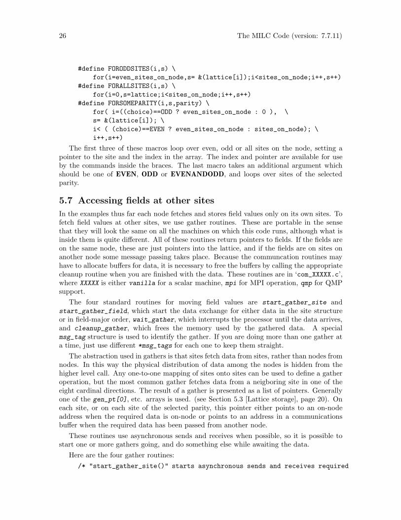
The first three of these macros loop over even, odd or all sites on the node, setting apointer to the site and the index in the array. The index and pointer are available for useby the commands inside the braces. The last macro takes an additional argument whichshould be one of EVEN, ODD or EVENANDODD, and loops over sites of the selectedparity.
5.7 Accessing fields at other sites
In the examples thus far each node fetches and stores field values only on its own sites. Tofetch field values at other sites, we use gather routines. These are portable in the sensethat they will look the same on all the machines on which this code runs, although what isinside them is quite different. All of these routines return pointers to fields. If the fields areon the same node, these are just pointers into the lattice, and if the fields are on sites onanother node some message passing takes place. Because the communcation routines mayhave to allocate buffers for data, it is necessary to free the buffers by calling the appropriatecleanup routine when you are finished with the data. These routines are in ‘com_XXXXX.c’,where XXXXX is either vanilla for a scalar machine, mpi for MPI operation, qmp for QMPsupport.
The four standard routines for moving field values are start_gather_site andstart_gather_field, which start the data exchange for either data in the site structureor in field-major order, wait_gather, which interrupts the processor until the data arrives,and cleanup_gather, which frees the memory used by the gathered data. A specialmsg_tag structure is used to identify the gather. If you are doing more than one gather ata time, just use different *msg_tags for each one to keep them straight.
The abstraction used in gathers is that sites fetch data from sites, rather than nodes fromnodes. In this way the physical distribution of data among the nodes is hidden from thehigher level call. Any one-to-one mapping of sites onto sites can be used to define a gatheroperation, but the most common gather fetches data from a neigboring site in one of theeight cardinal directions. The result of a gather is presented as a list of pointers. Generallyone of the gen_pt[0], etc. arrays is used. (see Section 5.3 [Lattice storage], page 20). Oneach site, or on each site of the selected parity, this pointer either points to an on-nodeaddress when the required data is on-node or points to an address in a communicationsbuffer when the required data has been passed from another node.
These routines use asynchronous sends and receives when possible, so it is possible tostart one or more gathers going, and do something else while awaiting the data.
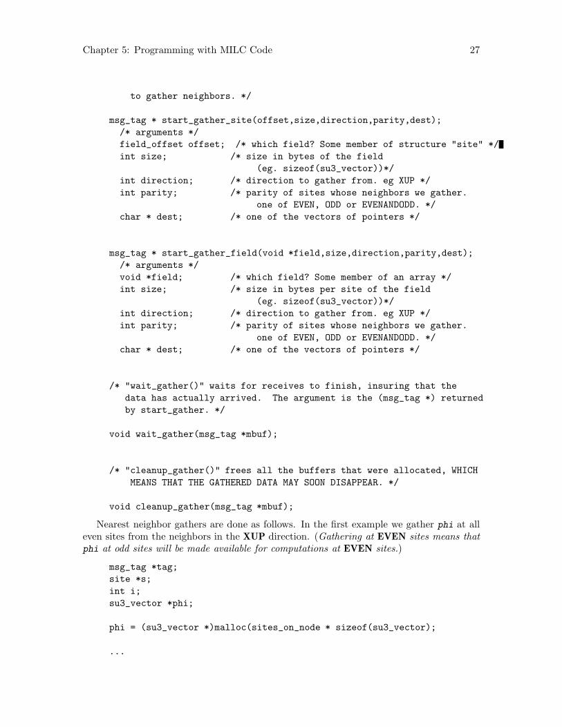
Here are the four gather routines:
/* "start_gather_site()" starts asynchronous sends and receives required
Chapter 5: Programming with MILC Code 27
to gather neighbors. */
msg_tag * start_gather_site(offset,size,direction,parity,dest);
/* arguments */
field_offset offset; /* which field? Some member of structure "site" */
int size; /* size in bytes of the field
(eg. sizeof(su3_vector))*/
int direction; /* direction to gather from. eg XUP */
int parity; /* parity of sites whose neighbors we gather.
one of EVEN, ODD or EVENANDODD. */
char * dest; /* one of the vectors of pointers */
msg_tag * start_gather_field(void *field,size,direction,parity,dest);
/* arguments */
void *field; /* which field? Some member of an array */
int size; /* size in bytes per site of the field
(eg. sizeof(su3_vector))*/
int direction; /* direction to gather from. eg XUP */
int parity; /* parity of sites whose neighbors we gather.
one of EVEN, ODD or EVENANDODD. */
char * dest; /* one of the vectors of pointers */
/* "wait_gather()" waits for receives to finish, insuring that the
data has actually arrived. The argument is the (msg_tag *) returned
by start_gather. */
void wait_gather(msg_tag *mbuf);
/* "cleanup_gather()" frees all the buffers that were allocated, WHICH
MEANS THAT THE GATHERED DATA MAY SOON DISAPPEAR. */
void cleanup_gather(msg_tag *mbuf);
Nearest neighbor gathers are done as follows. In the first example we gather phi at alleven sites from the neighbors in the XUP direction. (Gathering at EVEN sites means thatphi at odd sites will be made available for computations at EVEN sites.)
msg_tag *tag;
site *s;
int i;
su3_vector *phi;
phi = (su3_vector *)malloc(sites_on_node * sizeof(su3_vector);
...
28 The MILC Code (version: 7.7.11)
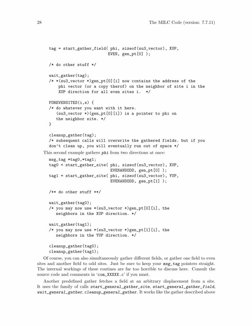
tag = start_gather_field( phi, sizeof(su3_vector), XUP,
EVEN, gen_pt[0] );
/* do other stuff */
wait_gather(tag);
/* *(su3_vector *)gen_pt[0][i] now contains the address of the
phi vector (or a copy therof) on the neighbor of site i in the
XUP direction for all even sites i. */
FOREVENSITES(i,s) {
/* do whatever you want with it here.
(su3_vector *)(gen_pt[0][i]) is a pointer to phi on
the neighbor site. */
}
cleanup_gather(tag);
/* subsequent calls will overwrite the gathered fields. but if you
don’t clean up, you will eventually run out of space */
This second example gathers phi from two directions at once:
msg_tag *tag0,*tag1;
tag0 = start_gather_site( phi, sizeof(su3_vector), XUP,
EVENANDODD, gen_pt[0] );
tag1 = start_gather_site( phi, sizeof(su3_vector), YUP,
EVENANDODD, gen_pt[1] );
/** do other stuff **/
wait_gather(tag0);
/* you may now use *(su3_vector *)gen_pt[0][i], the
neighbors in the XUP direction. */
wait_gather(tag1);
/* you may now use *(su3_vector *)gen_pt[1][i], the
neighbors in the YUP direction. */
cleanup_gather(tag0);
cleanup_gather(tag1);
Of course, you can also simultaneously gather different fields, or gather one field to evensites and another field to odd sites. Just be sure to keep your msg_tag pointers straight.The internal workings of these routines are far too horrible to discuss here. Consult thesource code and comments in ‘com_XXXXX.c’ if you must.
Another predefined gather fetches a field at an arbitrary displacement from a site.It uses the family of calls start_general_gather_site, start_general_gather_field,wait_general_gather, cleanup_general_gather. It works like the gather described above
Chapter 5: Programming with MILC Code 29
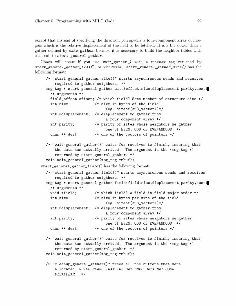
except that instead of specifying the direction you specify a four-component array of inte-gers which is the relative displacement of the field to be fetched. It is a bit slower than agather defined by make_gather, because it is necessary to build the neighbor tables witheach call to start_general_gather.
Chaos will ensue if you use wait_gather() with a message tag returned bystart_general_gather_XXXX(), or vice-versa. start_general_gather_site() has thefollowing format:
/* "start_general_gather_site()" starts asynchronous sends and receives
required to gather neighbors. */
msg_tag * start_general_gather_site(offset,size,displacement,parity,dest)
/* arguments */
field_offset offset; /* which field? Some member of structure site */
int size; /* size in bytes of the field
(eg. sizeof(su3_vector))*/
int *displacement; /* displacement to gather from,
a four component array */
int parity; /* parity of sites whose neighbors we gather.
one of EVEN, ODD or EVENANDODD. */
char ** dest; /* one of the vectors of pointers */
/* "wait_general_gather()" waits for receives to finish, insuring that
the data has actually arrived. The argument is the (msg_tag *)
returned by start_general_gather. */
void wait_general_gather(msg_tag *mbuf);
start_general_gather_field() has the following format:
/* "start_general_gather_field()" starts asynchronous sends and receives
required to gather neighbors. */
msg_tag * start_general_gather_field(field,size,displacement,parity,dest)
/* arguments */
void *field; /* which field? A field in field-major order */
int size; /* size in bytes per site of the field
(eg. sizeof(su3_vector))*/
int *displacement; /* displacement to gather from,
a four component array */
int parity; /* parity of sites whose neighbors we gather.
one of EVEN, ODD or EVENANDODD. */
char ** dest; /* one of the vectors of pointers */
/* "wait_general_gather()" waits for receives to finish, insuring that
the data has actually arrived. The argument is the (msg_tag *)
returned by start_general_gather. */
void wait_general_gather(msg_tag *mbuf);
/* "cleanup_general_gather()" frees all the buffers that were
allocated, WHICH MEANS THAT THE GATHERED DATA MAY SOON
DISAPPEAR. */
30 The MILC Code (version: 7.7.11)
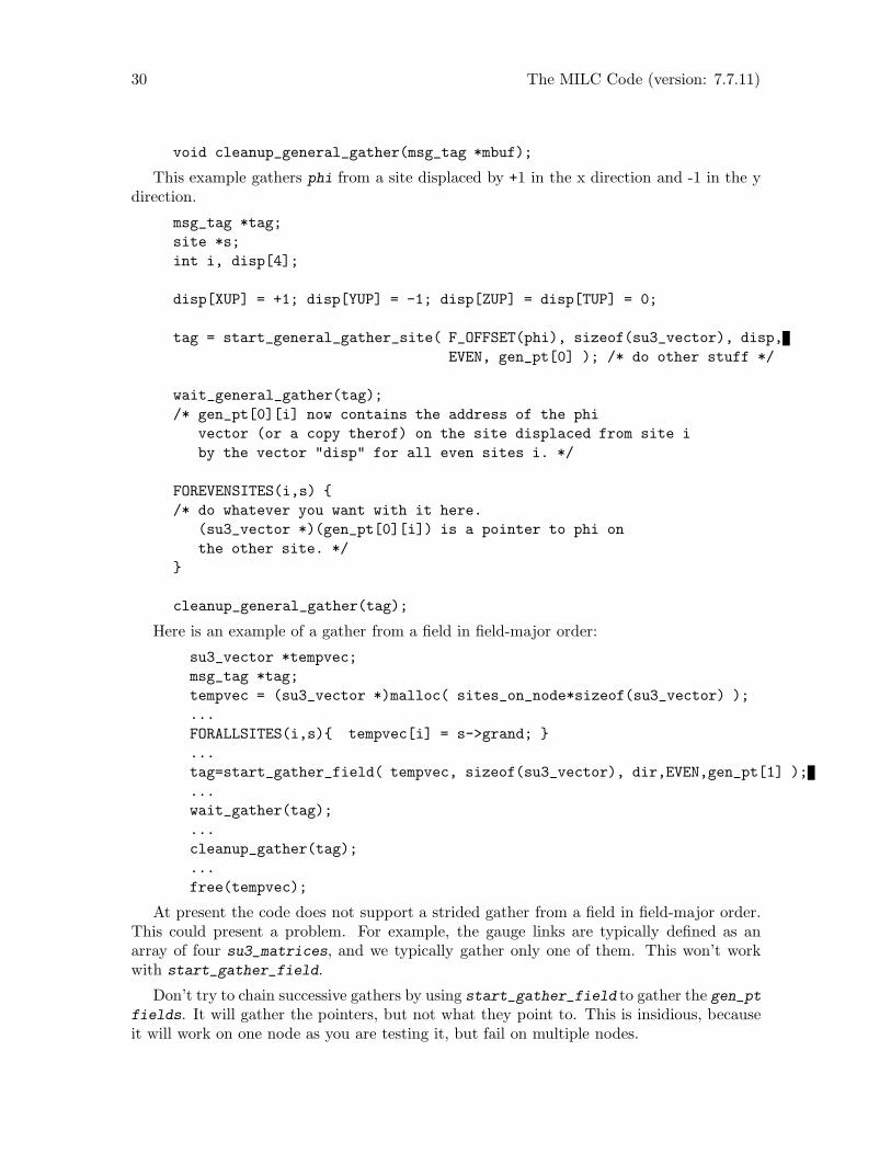
void cleanup_general_gather(msg_tag *mbuf);
This example gathers phi from a site displaced by +1 in the x direction and -1 in the ydirection.
msg_tag *tag;
site *s;
int i, disp[4];
disp[XUP] = +1; disp[YUP] = -1; disp[ZUP] = disp[TUP] = 0;
tag = start_general_gather_site( F_OFFSET(phi), sizeof(su3_vector), disp,
EVEN, gen_pt[0] ); /* do other stuff */
wait_general_gather(tag);
/* gen_pt[0][i] now contains the address of the phi
vector (or a copy therof) on the site displaced from site i
by the vector "disp" for all even sites i. */
FOREVENSITES(i,s) {
/* do whatever you want with it here.
(su3_vector *)(gen_pt[0][i]) is a pointer to phi on
the other site. */
}
cleanup_general_gather(tag);
Here is an example of a gather from a field in field-major order:
su3_vector *tempvec;
msg_tag *tag;
tempvec = (su3_vector *)malloc( sites_on_node*sizeof(su3_vector) );
...
FORALLSITES(i,s){ tempvec[i] = s->grand; }
...
tag=start_gather_field( tempvec, sizeof(su3_vector), dir,EVEN,gen_pt[1] );
...
wait_gather(tag);
...
cleanup_gather(tag);
...
free(tempvec);
At present the code does not support a strided gather from a field in field-major order.This could present a problem. For example, the gauge links are typically defined as anarray of four su3_matrices, and we typically gather only one of them. This won’t workwith start_gather_field.
Don’t try to chain successive gathers by using start_gather_field to gather the gen_ptfields. It will gather the pointers, but not what they point to. This is insidious, becauseit will work on one node as you are testing it, but fail on multiple nodes.
Chapter 5: Programming with MILC Code 31
To set up the data structures required by the gather routines, make_nn_gathers() iscalled in the setup part of the program. This must be done after the call to make_lattice().
5.8 Details of gathers and creating new ones
(You don’t need to read this section the first time through.)
The nearest-neighbor and fixed-displacement gathers are always available at run time,but a user can make other gathers using the make_gather routine. Examples of suchgathers are the bit-reverse and butterfly maps used in FFT’s. The only requirement is thatthe gather pattern must correspond to a one-to-one map of sites onto sites. make_gather
speeds up gathers by preparing tables on each node containing information about what sitesmust be sent to other nodes or received from other nodes. The call to this routine is:
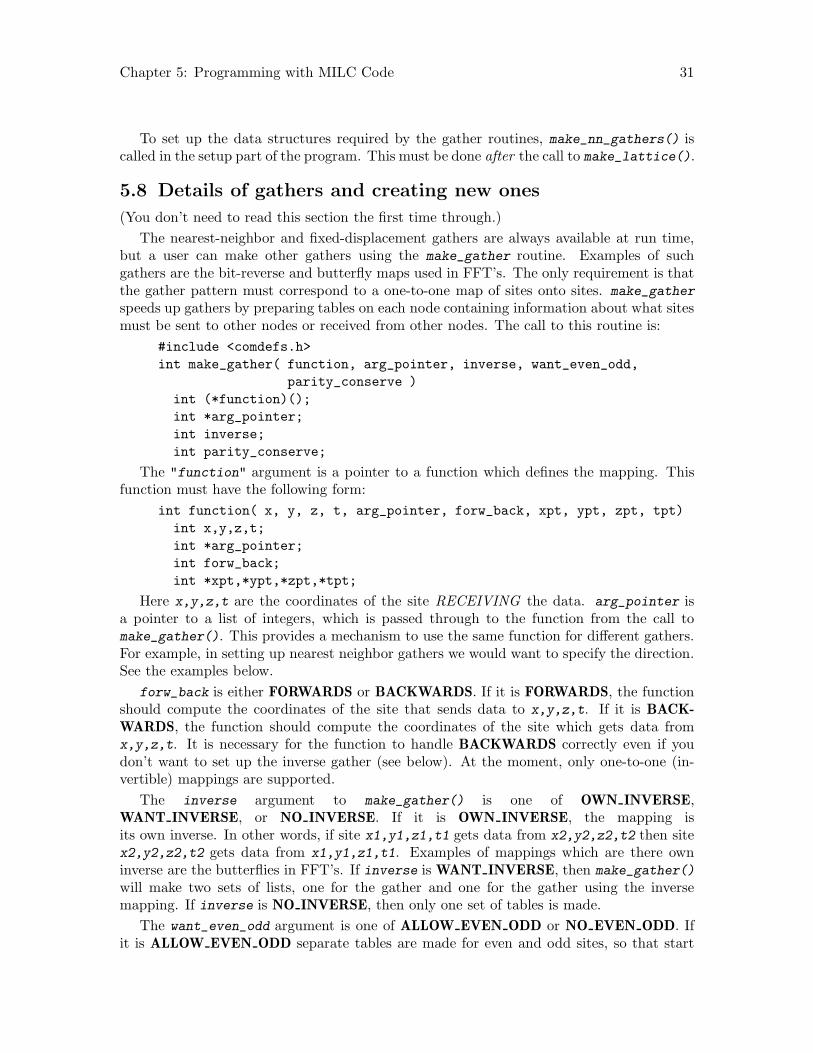
#include <comdefs.h>
int make_gather( function, arg_pointer, inverse, want_even_odd,
parity_conserve )
int (*function)();
int *arg_pointer;
int inverse;
int parity_conserve;
The "function" argument is a pointer to a function which defines the mapping. Thisfunction must have the following form:
int function( x, y, z, t, arg_pointer, forw_back, xpt, ypt, zpt, tpt)
int x,y,z,t;
int *arg_pointer;
int forw_back;
int *xpt,*ypt,*zpt,*tpt;
Here x,y,z,t are the coordinates of the site RECEIVING the data. arg_pointer isa pointer to a list of integers, which is passed through to the function from the call tomake_gather(). This provides a mechanism to use the same function for different gathers.For example, in setting up nearest neighbor gathers we would want to specify the direction.See the examples below.
forw_back is either FORWARDS or BACKWARDS. If it is FORWARDS, the functionshould compute the coordinates of the site that sends data to x,y,z,t. If it is BACK-WARDS, the function should compute the coordinates of the site which gets data fromx,y,z,t. It is necessary for the function to handle BACKWARDS correctly even if youdon’t want to set up the inverse gather (see below). At the moment, only one-to-one (in-vertible) mappings are supported.
The inverse argument to make_gather() is one of OWN INVERSE,WANT INVERSE, or NO INVERSE. If it is OWN INVERSE, the mapping isits own inverse. In other words, if site x1,y1,z1,t1 gets data from x2,y2,z2,t2 then sitex2,y2,z2,t2 gets data from x1,y1,z1,t1. Examples of mappings which are there owninverse are the butterflies in FFT’s. If inverse is WANT INVERSE, then make_gather()
will make two sets of lists, one for the gather and one for the gather using the inversemapping. If inverse is NO INVERSE, then only one set of tables is made.
The want_even_odd argument is one of ALLOW EVEN ODD or NO EVEN ODD. Ifit is ALLOW EVEN ODD separate tables are made for even and odd sites, so that start
32 The MILC Code (version: 7.7.11)
gather can be called with parity EVEN, ODD or EVENANDODD. If it is NO EVEN ODD,only one set of tables is made and you can only call gathers with parity EVENANDODD.
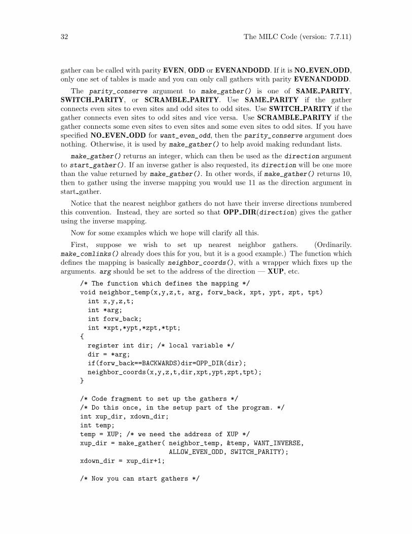
The parity_conserve argument to make_gather() is one of SAME PARITY,SWITCH PARITY, or SCRAMBLE PARITY. Use SAME PARITY if the gatherconnects even sites to even sites and odd sites to odd sites. Use SWITCH PARITY if thegather connects even sites to odd sites and vice versa. Use SCRAMBLE PARITY if thegather connects some even sites to even sites and some even sites to odd sites. If you havespecified NO EVEN ODD for want_even_odd, then the parity_conserve argument doesnothing. Otherwise, it is used by make_gather() to help avoid making redundant lists.
make_gather() returns an integer, which can then be used as the direction argumentto start_gather(). If an inverse gather is also requested, its direction will be one morethan the value returned by make_gather(). In other words, if make_gather() returns 10,then to gather using the inverse mapping you would use 11 as the direction argument instart gather.
Notice that the nearest neighbor gathers do not have their inverse directions numberedthis convention. Instead, they are sorted so that OPP DIR(direction) gives the gatherusing the inverse mapping.
Now for some examples which we hope will clarify all this.
First, suppose we wish to set up nearest neighbor gathers. (Ordinarily.make_comlinks() already does this for you, but it is a good example.) The function whichdefines the mapping is basically neighbor_coords(), with a wrapper which fixes up thearguments. arg should be set to the address of the direction — XUP, etc.
/* The function which defines the mapping */
void neighbor_temp(x,y,z,t, arg, forw_back, xpt, ypt, zpt, tpt)
int x,y,z,t;
int *arg;
int forw_back;
int *xpt,*ypt,*zpt,*tpt;
{
register int dir; /* local variable */
dir = *arg;
if(forw_back==BACKWARDS)dir=OPP_DIR(dir);
neighbor_coords(x,y,z,t,dir,xpt,ypt,zpt,tpt);
}
/* Code fragment to set up the gathers */
/* Do this once, in the setup part of the program. */
int xup_dir, xdown_dir;
int temp;
temp = XUP; /* we need the address of XUP */
xup_dir = make_gather( neighbor_temp, &temp, WANT_INVERSE,
ALLOW_EVEN_ODD, SWITCH_PARITY);
xdown_dir = xup_dir+1;
/* Now you can start gathers */
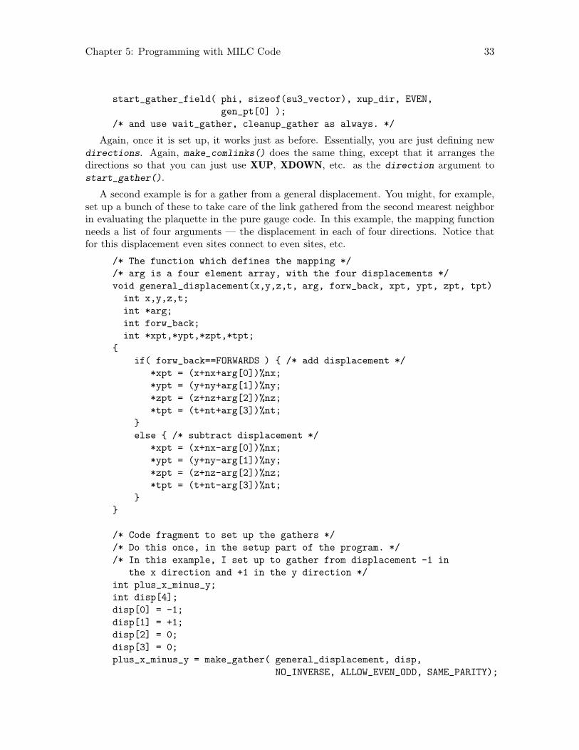
Chapter 5: Programming with MILC Code 33
start_gather_field( phi, sizeof(su3_vector), xup_dir, EVEN,
gen_pt[0] );
/* and use wait_gather, cleanup_gather as always. */
Again, once it is set up, it works just as before. Essentially, you are just defining newdirections. Again, make_comlinks() does the same thing, except that it arranges thedirections so that you can just use XUP, XDOWN, etc. as the direction argument tostart_gather().
A second example is for a gather from a general displacement. You might, for example,set up a bunch of these to take care of the link gathered from the second mearest neighborin evaluating the plaquette in the pure gauge code. In this example, the mapping functionneeds a list of four arguments — the displacement in each of four directions. Notice thatfor this displacement even sites connect to even sites, etc.
/* The function which defines the mapping */
/* arg is a four element array, with the four displacements */
void general_displacement(x,y,z,t, arg, forw_back, xpt, ypt, zpt, tpt)
int x,y,z,t;
int *arg;
int forw_back;
int *xpt,*ypt,*zpt,*tpt;
{
if( forw_back==FORWARDS ) { /* add displacement */
*xpt = (x+nx+arg[0])%nx;
*ypt = (y+ny+arg[1])%ny;
*zpt = (z+nz+arg[2])%nz;
*tpt = (t+nt+arg[3])%nt;
}
else { /* subtract displacement */
*xpt = (x+nx-arg[0])%nx;
*ypt = (y+ny-arg[1])%ny;
*zpt = (z+nz-arg[2])%nz;
*tpt = (t+nt-arg[3])%nt;
}
}
/* Code fragment to set up the gathers */
/* Do this once, in the setup part of the program. */
/* In this example, I set up to gather from displacement -1 in
the x direction and +1 in the y direction */
int plus_x_minus_y;
int disp[4];
disp[0] = -1;
disp[1] = +1;
disp[2] = 0;
disp[3] = 0;
plus_x_minus_y = make_gather( general_displacement, disp,
NO_INVERSE, ALLOW_EVEN_ODD, SAME_PARITY);
34 The MILC Code (version: 7.7.11)
/* Now you can start gathers */
start_gather_site( F_OFFSET(link[YUP]), sizeof(su3_matrix), plus_x_minus_y,
EVEN, gen_pt[0] );
/* and use wait_gather, cleanup_gather as always. */
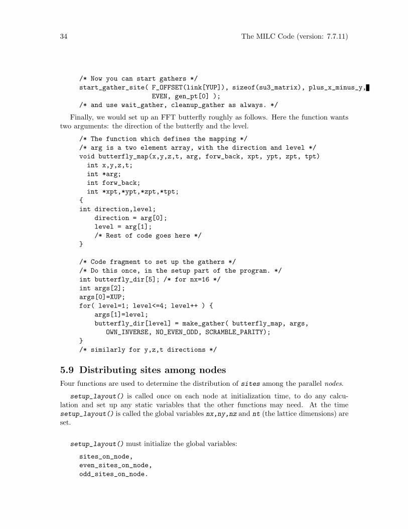
Finally, we would set up an FFT butterfly roughly as follows. Here the function wantstwo arguments: the direction of the butterfly and the level.
/* The function which defines the mapping */
/* arg is a two element array, with the direction and level */
void butterfly_map(x,y,z,t, arg, forw_back, xpt, ypt, zpt, tpt)
int x,y,z,t;
int *arg;
int forw_back;
int *xpt,*ypt,*zpt,*tpt;
{
int direction,level;
direction = arg[0];
level = arg[1];
/* Rest of code goes here */
}
/* Code fragment to set up the gathers */
/* Do this once, in the setup part of the program. */
int butterfly_dir[5]; /* for nx=16 */
int args[2];
args[0]=XUP;
for( level=1; level<=4; level++ ) {
args[1]=level;
butterfly_dir[level] = make_gather( butterfly_map, args,
OWN_INVERSE, NO_EVEN_ODD, SCRAMBLE_PARITY);
}
/* similarly for y,z,t directions */
5.9 Distributing sites among nodes
Four functions are used to determine the distribution of sites among the parallel nodes.
setup_layout() is called once on each node at initialization time, to do any calcu-lation and set up any static variables that the other functions may need. At the timesetup_layout() is called the global variables nx,ny,nz and nt (the lattice dimensions) areset.
setup_layout() must initialize the global variables:
sites_on_node,
even_sites_on_node,
odd_sites_on_node.
Chapter 5: Programming with MILC Code 35
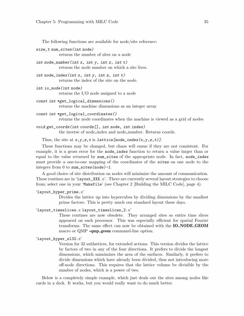
The following functions are available for node/site reference:
size_t num_sites(int node)
returns the number of sites on a node
int node_number(int x, int y, int z, int t)
returns the node number on which a site lives.
int node_index(int x, int y, int z, int t)
returns the index of the site on the node.
int io_node(int node)
returns the I/O node assigned to a node
const int *get_logical_dimensions()
returns the machine dimensions as an integer array
const int *get_logical_coordinates()
returns the node coordinates when the machine is viewed as a grid of nodes
void get_coords(int coords[], int node, int index)
the inverse of node index and node number. Returns coords.
Thus, the site at x,y,z,t is lattice[node_index(x,y,z,t)].
These functions may be changed, but chaos will ensue if they are not consistent. Forexample, it is a gross error for the node_index function to return a value larger than orequal to the value returned by num_sites of the appropriate node. In fact, node_indexmust provide a one-to-one mapping of the coordinates of the sites on one node to theintegers from 0 to num_sites(node)-1.
A good choice of site distribution on nodes will minimize the amount of communication.These routines are in ‘layout_XXX.c’. There are currently several layout strategies to choosefrom; select one in your ‘Makefile’ (see Chapter 2 [Building the MILC Code], page 4).
‘layout_hyper_prime.c’Divides the lattice up into hypercubes by dividing dimensions by the smallestprime factors. This is pretty much our standard layout these days.
‘layout_timeslices.c layout_timeslices_2.c’These routines are now obsolete. They arranged sites so entire time slicesappeared on each processor. This was especially efficient for spatial Fouriertransforms. The same effect can now be obtained with the IO NODE GEOMmacro or QMP -qmp geom command-line option.
‘layout_hyper_sl32.c’Version for 32 sublattices, for extended actions. This version divides the latticeby factors of two in any of the four directions. It prefers to divide the longestdimensions, which mimimizes the area of the surfaces. Similarly, it prefers todivide dimensions which have already been divided, thus not introducing moreoff-node directions. This requires that the lattice volume be divisible by thenumber of nodes, which is a power of two.
Below is a completely simple example, which just deals out the sites among nodes likecards in a deck. It works, but you would really want to do much better.
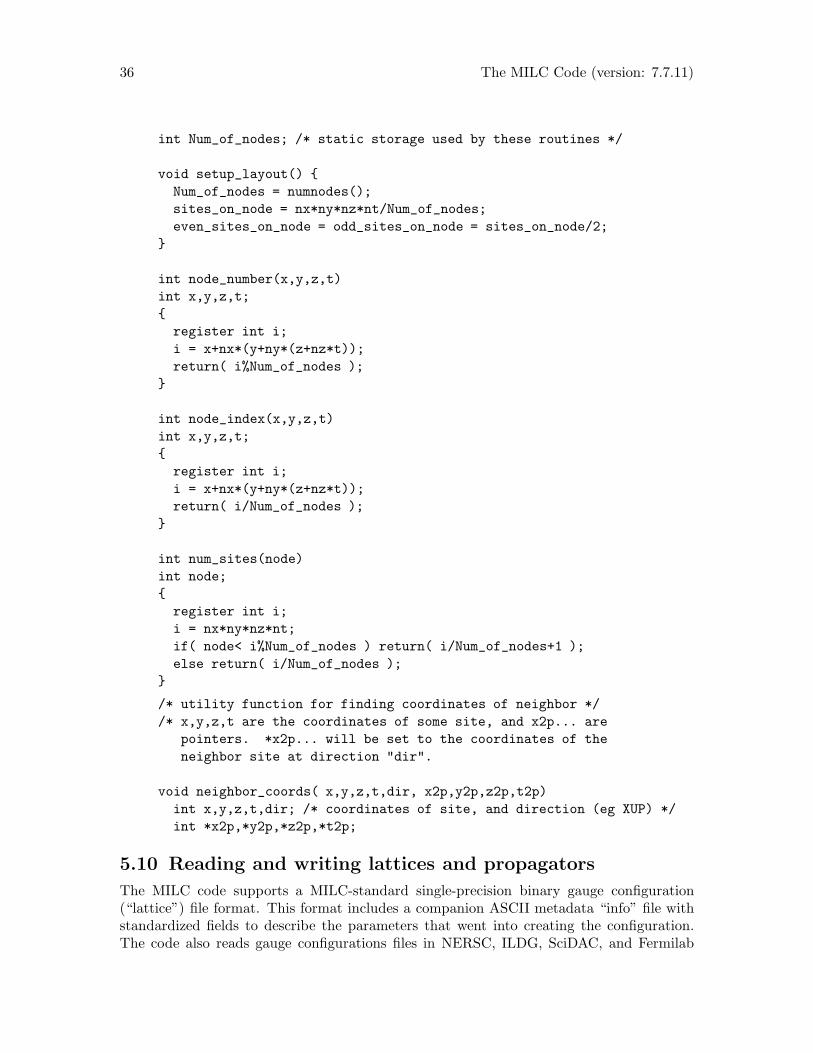
36 The MILC Code (version: 7.7.11)
int Num_of_nodes; /* static storage used by these routines */
void setup_layout() {
Num_of_nodes = numnodes();
sites_on_node = nx*ny*nz*nt/Num_of_nodes;
even_sites_on_node = odd_sites_on_node = sites_on_node/2;
}
int node_number(x,y,z,t)
int x,y,z,t;
{
register int i;
i = x+nx*(y+ny*(z+nz*t));
return( i%Num_of_nodes );
}
int node_index(x,y,z,t)
int x,y,z,t;
{
register int i;
i = x+nx*(y+ny*(z+nz*t));
return( i/Num_of_nodes );
}
int num_sites(node)
int node;
{
register int i;
i = nx*ny*nz*nt;
if( node< i%Num_of_nodes ) return( i/Num_of_nodes+1 );
else return( i/Num_of_nodes );
}
/* utility function for finding coordinates of neighbor */
/* x,y,z,t are the coordinates of some site, and x2p... are
pointers. *x2p... will be set to the coordinates of the
neighbor site at direction "dir".
void neighbor_coords( x,y,z,t,dir, x2p,y2p,z2p,t2p)
int x,y,z,t,dir; /* coordinates of site, and direction (eg XUP) */
int *x2p,*y2p,*z2p,*t2p;
5.10 Reading and writing lattices and propagators
The MILC code supports a MILC-standard single-precision binary gauge configuration(“lattice”) file format. This format includes a companion ASCII metadata “info” file withstandardized fields to describe the parameters that went into creating the configuration.The code also reads gauge configurations files in NERSC, ILDG, SciDAC, and Fermilab

Chapter 5: Programming with MILC Code 37
formats and writes files in NERSC, ILDG, and SciDAC formats. For MILC, ILDG, andSciDAC formats, it supports reading and writing either serially through node 0 or in parallelto and from a single file. There is also an historic but seldom-used provision for reading andwriting ASCII gauge configuration files. Through SciDAC QIO the MILC code supportsparallel reading and writing of multiple partitioned SciDAC file formats.
The MILC code supports the USQCD Dirac and staggered propagator file formatsthrough QIO. It also supports reading and writing two standard Fermilab propagator fileformats.
Input and output types are set at run time. Here is a summary of the I/O choices forgauge configuration files:
reload_ascii
reload_serial
Binary read by node 0. File format is autodetected.
reload_parallel
Binary read by all nodes. Only where hardware is available.
save_ascii
save_serial
Binary through node 0 - standard index order
save_parallel
Binary parallel - standard index order. Only where hardware is available.
save_checkpoint
Binary parallel - node dump order
save_serial_archive
NERSC Gauge Connection format. For the moment a parallel version is notavailable.
save_serial_scidac
save_parallel_scidac
save_serial_ildg
SciDAC single-file format and ILDG-compatible format.
save_partition_scidac
save_partition_ildg
SciDAC partition file format and ILDG-compatible partition file format.
save_multifile_scidac
save_multifile_ildg
SciDAC multifile format. (Node dump order, intended for temporary storage,rather than archiving.)
For Dirac propagators the old MILC-standard format has been abandoned in favor ofthe USQCD and Fermilab formats. Here is a summary of Dirac propagator I/O choices:
reload_ascii_wprop
reload_serial_wprop
Binary read by node 0. File format is autodetected.
38 The MILC Code (version: 7.7.11)
reload_parallel_wprop
Binary read by all nodes. Only where hardware is available.
save_ascii_wprop
save_serial_scidac_wprop
Binary through node 0 - standard index order
save_parallel_scidac_wprop
Binary parallel - standard index order. Only where hardware is available.
save_partfile_scidac_wprop
Binary parallel with multiple files.
save_multifile_scidac_wprop
Binary parallel with multiple files - node dump order
save_serial_fm_wprop
save_serial_fm_sc_wprop
Fermilab formats
For staggered propagators the code supports a MILC-standard format as well as theUSQCD formats and the Fermilab format. Here is a summary of Dirac propagator I/Ochoices:
reload_ascii_ksprop
reload_serial_ksprop
Binary read by node 0. File format is autodetected.
reload_parallel_ksprop
Binary read by all nodes. Only where hardware is available.
save_ascii_ksprop
save_serial_ksprop
Binary through node 0 - standard index order
save_serial_scidac_ksprop
Binary through node 0 - standard index order
save_parallel_scidac_ksprop
Binary parallel - standard index order. Only where hardware is available.
save_partfile_scidac_ksprop
Binary parallel with multiple files.
save_multifile_scidac_ksprop
Binary parallel with multiple files - node dump order
save_serial_fm_ksprop
Fermilab format.
To print out variables for debugging purposes, the library routines dumpvec, dumpmatand dump_wvec (for SU(3) vectors, SU(3) matrices and Wilson vectors) are quite useful:
FORALLSITES(i,s) {
if(magsq_wvec(&(s->psi)) > 1.e-10) {
Chapter 5: Programming with MILC Code 39
printf("%d %d %d %d\n", s->x, s->y, s->z,s->t);
printf("psi\n");
dump_wvec(&(s->psi));
}
}
5.11 Random numbers
The random number generator is the exclusive-OR of a 127 bit feedback shift register anda 32 bit integer congruence generator. It is supposed to be machine independent. Eachnode or site uses a different multipler in the congruence generator and different initial statein the shift register, so all are generating different sequences of numbers. If SITERANDis defined, which has become standard practice in our code, each lattice site has its ownrandom number generator state. This takes extra storage, but means that the results of theprogram will be independent of the number of nodes or the distribution of the sites amongthe nodes. The random number routine is generic/ranstuff.c.
5.12 A Sample Applications Directory
An example of the files which make up an application are listed here. This list dependsvery much on which application of the program (Kogut-Susskind/Wilson? Thermodynam-ics/Spectrum?) is being built. The listing here is for the pure MILC code (non-SciDAC)compilation of the su3_spectrum target for the 2+1 asqtad action in the ks_imp_dyn ap-plication.
‘Make_template:’Contains instructions for compiling and linking. Three routines you can make,"su3 rmd", "su3 phi" and "su3 hmc", are programs for the R algorithm, thephi algorithm, or the hybrid Monte Carlo algorithm.
SOME HIGH LEVEL ROUTINES:
‘control.c’main program
‘../generic_ks/ranmom.c’generate Gaussian random momenta for the gauge fields
‘../generic_ks/grsource_imp.c’generate Gaussian random pseudofermion field
‘setup.c’ interpret parameter input
‘update.c’top-level molecular dynamics
‘update_h.c’update the gauge momenta
‘update_u.c’update the gauge fields
40 The MILC Code (version: 7.7.11)
HEADERS
‘defines.h’Required. Local macros common to all targets in an application. SITERANDshould be defined here. Other macros that are independent of the site structurecan also be defined here.
‘gauge_action.h’Defines the gauge action
‘ks_imp_includes.h’Function prototypes for all files in the ks_imp_dyn application directory.
‘lattice.h’Required. Defines the site structure and global variables.
‘lattice_qdp.h’Required. Used only for QDP support.
‘params.h’Required. Defines the parameter structure used in setup.c for passing inputparameters to the nodes.
‘quark_action.h’Defines the quark action
LOWER LEVEL ROUTINES
‘gauge_info.c’Print gauge info to file.
‘../generic/ape_smear.c’APE smearing
‘../generic/check_unitarity.c’Check unitarity
‘../generic/com_qmp.c’Communications
‘../generic/d_plaq4.c’Plaquette
‘../generic/field_utilities.c’Creation and destruction of fields
‘../generic/file_types_milc_usqcd.c’USQCD file type translation
‘../generic/gauge_force_imp.c’Gauge force
‘../generic/gauge_stuff.c’Construction of gauge force.
‘../generic/gauge_utilities.c’Gauge field creation and destruction
Chapter 5: Programming with MILC Code 41
‘../generic/gaugefix2.c’Gauge fixing
‘../generic/general_staple.c’General staple calculation
‘../generic/io_ansi.c’Interface for ANSI I/O
‘../generic/io_detect.c’File type recognition
‘../generic/io_helpers.c’Top level lattice I/O
‘../generic/io_lat4.c’Gauge field I/O
‘../generic/io_lat_utils.c’Gauge field I/O
‘../generic/io_scidac.c’SciDAC file I/O wrapper
‘../generic/io_scidac_types.c’File type recognition
‘../generic/layout_hyper_prime.c’Lattice layout
‘../generic/make_lattice.c’Lattice creation
‘../generic/momentum_twist.c’Momentum twist insertion, removal
‘../generic/nersc_cksum.c’NERSC-type checksum
‘../generic/path_product.c’Paralle transport along path
‘../generic/ploop3.c’Polyakov loop
‘../generic/project_su3_hit.c’SU(3) projection
‘../generic/ranstuff.c’Random number generator
‘../generic/remap_stdio_from_args.c’Standard I/O remapping
‘../generic/report_invert_status.c’Status report
42 The MILC Code (version: 7.7.11)
‘../generic/reunitarize2.c’Reunitarization of gauge links
‘../generic/show_generic_opts.c’List options turned on
‘../generic_ks/d_congrad5_fn.c’Conjugate gradient inverter - top level
‘../generic_ks/d_congrad5_fn_milc.c’MILC coded inverter - single mass
‘../generic_ks/d_congrad5_two_src.c’Two-source inverter
‘../generic_ks/d_congrad_opt.c’Inverter support
‘../generic_ks/dslash_fn_dblstore.c’Dslash
‘../generic_ks/f_meas.c’Scalar operators, such as psi-bar-psi
‘../generic_ks/fermion_force_asqtad.c’Fermion force
‘../generic_ks/fermion_force_fn_multi.c’Fermion force
‘../generic_ks/fermion_force_multi.c’Fermion force for multiple shifts
‘../generic_ks/fermion_links.c’Fermion link creation/destruction
‘../generic_ks/fermion_links_fn_load_milc.c’Asqtad link fattening
‘../generic_ks/fermion_links_fn_twist_milc.c’Boundary twist
‘../generic_ks/fermion_links_from_site.c’Wrapper for creating links from gauge field
‘../generic_ks/fermion_links_milc.c’Fermion link fattening
‘../generic_ks/ff_opt.c’Fermion force optimization
‘../generic_ks/fn_links_milc.c’Creation/destruction utilities for fermion links
‘../generic_ks/ks_action_paths.c’Link fattening path
Chapter 5: Programming with MILC Code 43
‘../generic_ks/ks_invert.c’Wrapper for staggered inversion
‘../generic_ks/ks_multicg.c’Multimass inverter - top level
‘../generic_ks/ks_multicg_offset.c’Multimass inverter
‘../generic_ks/mat_invert.c’Inverter for spectrum
‘../generic_ks/path_transport.c’Parallel transport
‘../generic_ks/rephase.c’Insert/remove KS phases
‘../generic_ks/show_generic_ks_md_opts.c’Show options in force
‘../generic_ks/show_generic_ks_opts.c’Show options in force
‘../generic_ks/show_hisq_force_opts.c’Show options in force
LIBRARIES
‘complex.1.a’complex number operations. See section on "Library routines".
‘su3.1.a’ 3x3 matrix and 3 component vector operations. See "utility subroutines".
5.13 Bugs and features
Some variants of the version 4 MILC code had library routines and applications for doingSU(2) gauge theory. This code has not been translated into version 7 conventions.
The MILC code is hard-wired for four dimensional simulations. Three and five dimen-sional variants are believed to exist, but are not maintained by us.
For some unknown reason, lost in the mists of time, the MILC code uses the oppositeconvention for the projectors
S =∑
x
ψ̄(x)ψ(x) − κ(∑
µ
ψ̄(x)(1 + γµ)Uµ(x)ψ(x + µ) +∑
µ
ψ̄(x+ µ)(1− γµ)U†µ(x)ψ(x))
rather than the more standard convention
S =∑
x
ψ̄(x)ψ(x) − κ(∑
µ
ψ̄(x)(1 − γµ)Uµ(x)ψ(x+ µ)) +∑
µ
ψ̄(x+ µ)(1 + γµ)U†µ(x)ψ(x))
Furthermore, the sign convention for γ2 is minus the standard convention. Thus the MILCspinor fields differ from the “conventional” ones by a gamma-5 multiplication ψMILC =γ5ψusual. and a reflection in the x-z plane. MILC uses Weyl-basis (gamma-5 diagonal)Dirac matrices.

44 The MILC Code (version: 7.7.11)
6 Writing Your Own Application
Each application typically uses at least four header files, APP_includes.h, lattice.h,defines.h and params.h. The first contains definitions of all the routines in the applicationdirectory; the second contains a list of global macros and global definitions and a specifi-cation of the site structure (all the variables living on the sites of your lattice); the thirdcontains local macros common to all targets in an application; and the last defines the pa-rameter structure used for passing input parameters to the nodes. The application directoryalso has its own makefile, Make_template, which contains all the (machine-independent)dependencies necessary for your applications.
It is customary to put the main() routine in a file which begins with the word “control”(e.g. control_clov_p.c). Beyond that, you are on your own. If you poke around, youmay find a routine similar to the one you want to write, which you can modify. A typicalapplication reads in a lattice reads in some input parameters, does things to variables onevery site, moves information from site to site (see Section 5.7 [Accessing fields at othersites], page 26) and writes out a lattice at the end.
One problem is how to read in global parameters (like a coupling or the number ofiterations of a process). This is done in a file with a name similar to setup.c. To read in aglobal variable and broadcast it to all the nodes, you must first edit lattice.h adding thevariable to the list of globals (in the long set of EXTERN’s at the top), and edit the params.hfile to add it to the params structure. Next, in setup.c, add a set of lines to prompt forthe input, and find the place where the params structure is initialized or read. Add yourvariable once to each list, to put it into par_buf, and then to extract it. Good luck!
Chapter 7: Documentation for Specific Applications 45
7 Documentation for Specific Applications
We provide, here, documentation for some of the applications.
7.1 clover invert2
This code generates Dirac clover and naive propagators from a wide variety of sources andties them together to form meson and baryon correlators. With extended sources, the codealso computes correlators needed fo three-point and higher functions. The code is designedto be flexible in specifying source interpolating operators, propagators, sink interpolatingoperators, and the combinations to form hadrons. In broad terms a “meson” is contructedby tying together quark and antiquark propagators. These quark propagators are generatedin a succession of steps. First a base source is defined. A base source can then be modified byapplying a sequence of source operators to complete the definition of the source interpolatingoperator. The propagator starts from the source and propagates to any sink location. Atthe sink a variety of operators can be applied to form the completed quark propagator.They are then used to form the hadrons.
Because of the high degree of flexibility in the code, the parameter input file is rathercomplex and highly structured. We explain the construction of the parameter input file insome detail here. Examples can be found in the directory clover invert2/test/*.sample-in.
The parameter input file consists of the following required parts in this order:
This complete set of commands can be repeated indefinitely to form a chain of consecutivecomputations.
For human readability, comments on lines beginning with hash (#) are allowed in theparameter input file. Blank lines are also permitted.
7.1.1 Geometry etc. specification
prompt <int>
Here, valid values of <int> are 0, 1, 2. The value 0 takes parameters from stdin withoutprompting. The value 1 takes parameters from stdin with stdout prompts. The value 2 isfor proofreading. The parameter input file is scanned but no computations take place.
nx <int>
ny <int>
nz <int>
nt <int>
These are the lattice dimensions.
node_geometry <int[4]>
If the code is compiled with the macro FIX NODE GEOM, the above line is required.Otherwise, it should be omitted. It sets up a mesh view of the machine based on themachine x y z t dimensions. The lattice nx ny nz nt dimensions are divided according tothese values. The product of the int[4] values must equal the number of cores to be used.
ionode_geometry <int[4]>
If the code is compiled with both FIX NODE GEOM and FIX IONODE GEOM de-fined, then the above line is required. It sets I/O partitions for SciDAC partfile operation.
46 The MILC Code (version: 7.7.11)
The values 1 1 1 1 put the entire machine into one I/O partition, so only one partfile iswritten/read. Copying the values in node geometry puts each core in its own I/O par-tition, so resulting in as many partfiles read/written as there are cores. Each value inionode geometry must be a divisor of the corresponding value in node geometry.
iseed <int>
This line sets the random number seed. It is needed for random wall sources.
job_id <char[]>
The Job ID is copied into the metadata in the output correlator files.
7.1.2 Gauge field specification
The gauge field specification has the following required components:
7.1.2.1 Gauge field input
The following choices are available. Use only one of these.
reload_serial <char[]> |
reload_parallal <char[]> |
reload_ascii <char[]> |
fresh |
continue
The <char[]> string is the path to the file. The file type is detected automatically. Sup-ported binary file types include MILCv5, SciDAC (USQCD), ILDG, NERSC, and FNAL-style. If the file is in SciDAC format in multiple parts with volume extensions volnnnnn,the path should omit the volume extension.
With serial reading only the I/O nodes read the file. With SciDAC singlefile format,there is only one I/O node, namely the master node. With SciDAC partfile format, eachI/O partition resulting from the ionode geometry specification has one I/O node and itreads its own partfiles serially. With parallel reading all nodes read the file. Currently,parallel reading is not supported for partfiles, but future versions of SciDAC QIO may doso.
Provision is made for reading a file in ASCII format, but this mode is never used forproduction running.
The fresh command specifies a gauge field consisting of unit matrices. The continuecommand is used when several computations are chained together. It retains the previouslyloaded gauge configuration.
7.1.2.2 Tadpole factor and gauge fixing
u0 <float>
This sets the tadpole factor.
coulomb_gauge_fix |
no_gauge_fix
This line specifies whether to fix to Coulomb gauge or not. Choose one of these.
Chapter 7: Documentation for Specific Applications 47
7.1.2.3 Gauge field output
forget |
save_ascii <char[]> |
save_serial <char[]> |
save_parallel <char[]> |
save_checkpoint <char[]> |
save_serial_fm <char[]> |
save_serial_scidac <char[]> |
save_parallel_scidac <char[]> |
save_multifile_scidac <char[]> |
save_partfile_scidac <char[]> |
save_serial_ildg <char[]> |
save_parallel_ildg <char[]> |
save_multifile_ildg <char[]> |
save_partfile_ildg <char[]>
Choose one of these for saving the gauge configuration to a file. The command forgetdoes not save it. Otherwise, the <char[]> specifies the path to the file to be created.
The save serial, save parallel, and save checkpoint commands save the file in MILCv5format. The mode of writing is either serial (only the master node writes the file), parallel(all nodes write to a single file), and checkpoint (each node writes its own data to a separatefile.) The checkpoint format is deprecated. It is being replaced by the corresponding SciDACpartfile format.
The save serial fm command saves the file in Fermilab format.
The various scidac and ildg modes require compilation with QIO and QMP. The se-rial scidac mode writes to a single file through a single node. The parallel scidac modewrites to a single file with all nodes writing. The partfile scidac mode writes multiple part-files, one file per I/O partition. The multifile scidac mode writes a separate file for eachnode.
The ildgmode generates an ILDG-compatible file. It requires specifying the ILDG logicalfile name (LFN) on a separate line immediately following the save XXX ildg line:
ILDG_LFN <char[]>
7.1.2.4 APE smearing
staple_weight <float>
ape_iter <int>
Provision is made to smooth the input gauge field with the specified number of APEiterations using the specified weight. These lines are required even if smearing is not desired.In that case use zeros for each value.
7.1.2.5 Coordinate origin
Boundary conditions and momentum (“boundary”) twists for the Dirac operator depend onthe coordinate origin, which establishes which gauge links are on the boundary. It is commonpractice to boost statistics by computing the same hadron correlator from several originson the same gauge field configuration. It may be desirable to guarantee that the result isequivalent to applying a straight coordinate translation to the gauge field configuration and
48 The MILC Code (version: 7.7.11)
then computing propagators from an unshifted origin. The coordinate origin parameterdoes this
coordinate_origin <int[4]>
The order of coordinates is, as usual, x, y, z, and t.
7.1.3 Inversion control
max_cg_iterations <int>
max_cg_restarts <int>
These lines specify the maximum number of CG iterations allowed before restarting andthe maximum number of restarts. Thus the overall maximum number of iterations is theproduct of these two. Further inversion control is given below for each propagator.
7.1.4 Base sources
Here we describe the specification of the base sources. They are elementary and can beused by themselves or made more elaborate with modifications.
The definition starts by specifying the number of base sources, followed by that manystanzas describing the sources. Here we have used a hash (#) to introduce comments.Choices for the [source stanza] are explained below.
number_of_base_sources <int = n>
# source 0
[source_stanza]
# source 1
[source_stanza]
etc.
# source n-1
[source_stanza]
Each [source stanza] has the following structure. Items in brackets [] are explainedbelow.
<char[] source_name>
subset <full|corner>
[source_parameters]
[optional scale factor]
source_label <char[]>
[save_source_specification]
The source name can specify a complex field, a color vector field, or a dirac field (usuallydefined on a single time slice). For each source type the [source parameters] are specifiedas explained in more detail below. For a Dirac propagator, the spin and color content is
Chapter 7: Documentation for Specific Applications 49
completed by multiplying an appropriate spin-color unit vector by the specified complexfield. The possible choices and their [source parameters] are described in detail below.
The subset mask is applied to the base source and to any of its modifications. Thechoices are corner and full. With corner, after a source is constructed, the values on allsites are set to zero except on the corners of each 2^4 hypercube. With full, no mask isapplied. This mask is useful for naive and staggered fermion sources.
The [optional scale factor] has the form
scale_factor <float>
This line is read only if the code is compiled with the macro SCALE PROP defined. Itmultiplies the source by this factor, and then divides the resulting hadron correlators bythis factor to compensate, which should result in no visible modification of the result. It isuseful to prevent exponent underflow in computing propagators for especially heavy quarks.At the moment this factor is applied only to Dirac field sources.
The source label should be only a couple characters long, since it is used in constructinga name for the hadron correlator.
Provision is made for saving the source to a file. Currently, this happens only if thesource is actually used to calculate a propagator. The [save source specification] has thesyntax
forget_source |
save_serial_scidac_ks_source <char[]> |
save_multifile_scidac_ks_source <char[]> |
save_partfile_scidac_ks_source <char[]> |
save_serial_scidac_w_source <char[]> |
save_multifile_scidac_w_source <char[]> |
save_partfile_scidac_w_source <char[]>
These choices follow the same pattern as the choices for saving the gauge configuration,except they are more limited.
We turn now to a description of the various source types and their parameters. Complexfield source names can be any of the following:
A color vector field serves as the complete source for a naive propagator (which beginsits life as a staggered propagator). For a clover propagator, the spin content is completedby multipying the color field by an appropriate unit spin vector. Color vector field namesare any of the following:
Dirac field source names are any of the following:
7.1.4.1 complex field
origin <int[4]>
load_source <char[] = file_name>
momentum <int[3]>
These are the [source parameters] for the complex field source. This source is read froma file in SciDAC format. The source must be on a single time slice. The placement of thesource is controlled by the file, which must agree with the source origin on the origin line.(Typically, the source file was created in a previous calculation. In that case the originshould match the value in that calculation. If that calculation required only a value for the
50 The MILC Code (version: 7.7.11)
time slice coordinate t0, then use the origin 0 0 0 t0). The momentum line specifies a planewave factor that can modify the source. The integers specify the x, y, and z components ofthe momentum in units of 2 pi/nx, 2 pi/ny, and 2 pi/nz, respectively.
7.1.4.2 complex field fm
origin <int[4]>
load_source <char[] = file_name>
momentum <int[3]>
This source is similar to the complex field source, except the binary file is in Fermilabformat.
7.1.4.3 corner wall
t0 <int>
On the specified time slice this source is one at the origin of each 2^3 cube and zeroelsewhere.
7.1.4.4 even wall
t0 <int>
On the specified time slice this source is one on all even sites, i.e. with (x + y + z) even.
7.1.4.5 evenandodd wall
t0 <int>
On the specified time slice this source is one on all sites.
7.1.4.6 evenminusodd wall
t0 <int>
On the specified time slice this source is one on even sites and minus one on odd sites.
7.1.4.7 gaussian wall
origin <int[4]>
r0 <float>
A Gaussian profile source centered at the origin, specified by the integers x, y, z, t. Thissource has the value exp[−(r/r0)2] where r is the Cartesian displacement from x, y, z anthe fixed time slice t. This is a non-gauge-covariant source, so it is common to use it onlywith Coulomb gauge fixing.
7.1.4.8 point
origin <int[4]>
A point source of strength one at the origin specified by the integers x, y, z, and t.
7.1.4.9 wavefunction
origin <int[4]>
load_source <char[] = file_name>
a <float>
Chapter 7: Documentation for Specific Applications 51
momentum <int[3]>
Reads an ASCII wavefunction specified in physical coordinates (fm) and converts itto lattice coordinates for lattice spacing a. The wavefunction is centered at the origin,specified by four integers x, y, z, and t. A Fourier phase factor specified by the three integermomentum components multiplies the wave function.
7.1.4.10 random color wall
t0 <int>
ncolor <int>
momentum <int[3]>
Generates ncolor random color vector fields on the time slice t0. For a Dirac source thesame random source is used for each of the four associated spins. A Fourier phase factorspecified by the three integer momentum components multiplies the wave function.
7.1.4.11 vector field
origin <int[4]>
load_source <char[] = file_name>
ncolor <int>
momentum <int[3]>
Reads ncolor color vector sources from a file in SciDAC format. The oritin origin mustmatch the origin in the file. (Typically, the source file was created in a previous calculation.In that case the origin should match the value in that calculation. If that calculationrequired only a value for the time slice coordinate t0, then use the origin 0 0 0 t0). AFourier phase factor specified by the three integer momentum components multiplies thewave function.
7.1.4.12 vector field fm
origin <int[4]>
load_source <char[] = file_name>
ncolor <int>
momentum <int[3]>
Reads ncolor color vector sources from a file in Fermilab format. The origin origin mustmatch the origin in the file. (See the note for vector field for further explanation.) AFourier phase factor specified by the three integer momentum components multiplies thewave function.
7.1.4.13 vector propagator file
ncolor <int>
Our USQCD-formatted propagator files include the source fields with the solution fields.In this case the source field is to be taken from the file specified in the propagator stanzabelow.
7.1.4.14 dirac field
origin <int[4]>
load_source <char[] = file_name>
52 The MILC Code (version: 7.7.11)
nsource <int>
momentum <int[3]>
Reads nsource Dirac field sources from a file in SciDAC format. The origin origin mustmatch the origin in the file. (See the note for vector field for further explanation.) AFourier phase factor specified by the three integer momentum components multiplies thewave function.
The nsource Counts colors times spins, so it should be 12 for a conventional Dirac source.
7.1.4.15 dirac field fm
origin <int[4]>
load_source <char[] = file_name>
momentum <int[3]>
Reads exactly 12 Dirac field sources from a file in FNAL format. The origin originmust match the origin in the file. (See the note for vector field for further explanation.)A Fourier phase factor specified by the three integer momentum components multiplies thewave function.
7.1.4.16 dirac propagator file
nsource <int>
Our USQCD-formatted propagator files include the source fields with the solution fields.In this case the source field is to be taken from the file specified in the propagator stanzabelow. The number of source to use is specified by nsource.
7.1.5 Modified sources
The base sources described above can be used directly for computing propagators, but theycan also be modified. The modifications are defined by a sequence of operators acting onthe base sources and on the previously modified sources. The same operators are used atthe propagator sink, as described below. The only difference is that the source operatorsact on only the source time slice, whereas the sink operators act on all sink time slices.
The operator definition starts by specifying the number of modified sources, followedby that many stanzas describing the modifications. Choices for the [operator stanza] areexplained below.
At present all sources are referred to by integers. The enumeration of the sources isconsecutive from zero, starting with the base sources and continuing with the modifiedsources. Thus after n base sources the first modified source is source number n.
number_of_modified_sources <int = m>
# source n
[operator_stanza]
# source n+1
[operator_stanza]

Chapter 7: Documentation for Specific Applications 53
etc.
# source n+m-1
[operator_stanza]
Each [operator stanza] has the following structure. Items in brackets [] are explainedbelow.
<char[] operator_name>
source <int>
[operator_parameters]
op_label <char[]>
[save_source_specification]
Choices for operator name and the corresponding [operator parameteers] are describedin detail below.
The source line specifies the previous source upon which the operator acts. This sourcecan be either a previously defined base source or modified source.
The op label and [save source specification] are the same as for the base sources. Again,in the current code version, a request to save a source is ignored unless the source is alsoused to construct a propagator.
Here are possible choices for the [operator stanza]. As with the base sources, each hasits specific set of parameters.
The first set of operators specify convolutions with a complex field, which can be appliedto both staggered and Dirac fiels:
The second set apply covariant smearing and derivatives, which can also be applied toboth staggered and Dirac fiels:
The third set is peculiar to staggered fermions:
The fourth set is used only with Dirac fermions:
The fifth set is common to both Dirac and staggered fermions:
Here are the operators that do convolutions with a complex field:
7.1.5.1 complex field operator
load_source <char[]>
The complex field is contained the specified file (SciDAC format). The convolution takesplace on the time slice of the underlying source.
7.1.5.2 complex field fm operator
load_source <char[]>
Same as complex field, but the file is in FNAL format.
7.1.5.3 evenandodd wall operator
There are no additional parameters. This convolution is equivalent to a projection ontozero momentum. In other words it replaces the source value at each site on the underlyingsource time slice with the time-slice sum of the underlying source.
54 The MILC Code (version: 7.7.11)
7.1.5.4 gaussian
r0 <float>
The convolution uses a Gaussian of width r0 (centered at the origin). The conventionfor the width r0 is the same as for the gaussian base source.
7.1.5.5 identity operator
There are no parameters. This operator simply produces a copy. There should be no needto use it for sources, but it has a use as a sink operator, as described below.
7.1.5.6 wavefunction operator
wavefunction
load_source <char[]>
a <float>
This convolution uses the wave function in the specified ASCII file. As with the analogousbase source, the wave function is in physical (fm) units. It is converted to lattice units usinglattice spacing a.
7.1.5.7 covariant gaussian operator
r0 <float>
source_iters <int = n>
This operator applies a covariant Gaussian with the specified width and iterations. It isdefine by [1+r2
0D2/n]2 The discrete covariant Laplacian D2 is constructed from the original
unfattened gauge field.
7.1.5.8 deriv1 operator
dir <x|y|z>
disp <int = d>
weights <float[d]>
This operator applies a covariant finite difference in the direction specified by dir. Thedifference operation is specified by a template over 2d+1 lattice sites with the specifiedweights. So to get the central finite difference, use disp 1 and weights 1.
7.1.5.9 deriv2 D operator
dir <x|y|z> <x|y|z>
disp <int = d>
weights <fload[d]>
Computes a symmetric covariant second derivative based on the specified template anddirections. That is for dir x y the operation results in D x D y + D y D x, where D i isthe deriv1 operation above.
7.1.5.10 deriv2 B operator
dir <x|y|z> <x|y|z>
disp <int = d>
weights <float[d]>
Chapter 7: Documentation for Specific Applications 55
Computes an antisymmetric covariant second derivative based on the specified templateand directions. That is, for dir x y the operation results in D x D y - D y D x, where D iis the deriv1 operation above.
7.1.5.11 deriv3 A operator
disp <int = d>
weights <float[d]>
This operation is not yet supported.
7.1.5.12 fat covariant gaussian operator
r0 <float>
source_iters <int>
This operation is the same as covariant gaussian, except that the APE smeared linksare used. See the gauge-field description above for APE smearing.
7.1.5.13 funnywall1 operator
No parameters. This operation applies the staggered fermion “funnywall1” operator thatcouples to a subset of tastes. It is meaningful only for staggered fermion sources andpropagators.
7.1.5.14 funnywall2 operator
Same as above, but for the “funnywall2” operator.
7.1.5.15 ks inverse operator
ks_inverse
mass <float>
naik_term_epsilon <float>
u0 <float>
max_cg_iterations <int>
max_cg_restarts <int>
error_for_propagator <float>
rel_error_for_propagator <float>
precision <1|2>
coordinate_origin <int[4]>
momentum_twist <float[3]>
time_bc <antiperiodic|periodic>
Applies the inverse of the asqtad or HISQ Dirac operator.
7.1.5.16 spin taste operator
gamma pion5
Applies staggered spin-taste offsets and phases
7.1.5.17 ext src ks operator
spin_taste pion5
momentum <int[3]>
56 The MILC Code (version: 7.7.11)
t0 <int>
Projects a propagator to the specified time slice and applies the specified spin-tasteoperator and inserts the specified momentum.
7.1.5.18 rotate 3D operator
d1 <float>
This operator applies the FNAL 3D rotation to a Dirac source or sink.
7.1.5.19 dirac inverse operator
kappa <float>
clov_c <float>
u0 <float>
max_cg_iterations <int>
max_cg_restarts <int>
error_for_propagator <float>
rel_error_for_propagator <float>
precision <1|2>
coordinate_origin <int[4]>
momentum_twist <float[3]>
time_bc <antiperiodic|periodic>
This operator applies the inverse of the clover Dirac operator.
7.1.5.20 gamma operator
gamma G5
This operator multiplies by the specified gamma matrix.
7.1.5.21 ks gamma operator
Multiplies by the gamma matrix operator that reduces naive fermions to staggered fermions.
7.1.5.22 ks gamma inv operator
Multiplies by the inverse of the gamma matrix operator that reduces naive fermions tostaggered fermions.
7.1.5.23 ext src dirac operator
gamma G5
momentum <int[3]>
t0 <int>
Projects a propagator to the specified time slice and applies the specified gamma matrixoperator and inserts the specified momentum.
7.1.5.24 project t slice operator
t0 <int>
Projects values on the specified time slice.
Chapter 7: Documentation for Specific Applications 57
7.1.5.25 momentum operator
momentum <int[3]>
Multiplies by the plane-wave phase site-by-site.
7.1.5.26 modulation operator
file <char[]>
Reads the specified file containing a complex field and multiplies the values site-by-site.
7.1.6 Propagator description
Propagators are solutions to the inhomogeneous Dirac equation with either base or modifiedsources. These solutions can then be modified at the sink to implement appropriate sinkinterpolating operators. For simplicity we call the unmodified propagators “propagators”and the modified propagators “quarks”. The “quarks” are used to construct the hadronpropagators. Here we describe the “propagators”.
The code generates three classes of propagators, namely clover, naive, and “extendednaive”. The naive propagator is constructed starting from a (uually improved) staggeredpropagator, and multiplying by a spin matrix that reverses the Kawamoto-Smit staggeredspin rotation. The extended naive propagator is singled out because the source treatmentis special. It is intended for applications that generate a naive propagator from the specialextended Dirac sources produced by the ext src application. In that case four staggeredinversions are required for each Dirac source, one for each of the four spin components. Theextended Dirac source on a single time slice is usually the value on that time slice of a Diracpropagator that started propagation from an underlying source on a distant time slice. Sothere is one extended Dirac source for each spin and color of the underlying source. Thenumber of staggered inversions is therefore four times the number of underlying spins andcolors.
One must pay particular attention to the spin structure in the conversion from a stag-gered to a naive propagator. The spin matrix in the conversion depends on the sourceand sink 2^4 hypercube coordinates. The sink dependence is not problematic. The sourcedependence is, however. The conversion fails when the source for the staggered propagatorhas support on different hypercube sites. Thus, as a rule, the source for a naive propagatorshould be constructed with the subset corner mask, so it has support on only the hyper-cube origins. For the special case of an extended naive propagator, the spin conversion ispartially done in the ext src application and completed in the clover invert2 application.In this way the extended source can have support on all spatial sites on the source timeslice. If the extended source is not constructed by the ext src application, it, too, shouldbe restricted to the hypercube origins.
The propagators are specified in a manner similar to the sources. The number of prop-agators is specified, followed by that many stanzas, one for each propagator.
number_of_propagators <int p>
# propagator 0
[propagator_stanza]
58 The MILC Code (version: 7.7.11)
# propagator 1
[propagator_stanza]
...
# propagator p-1
[propagator_stanza]
The [propagator stanza] has the following structure;
[propagator_type]
[propagator_parameters]
check <yes|no>
error_for_propagator <float>
rel_error_for_propagator <float>
precision <1|2>
momentum_twist <float[3]>
time_bc <periodic|antiperiodic>
source <int>
[propagator input specification]
[propagator output specification]
There are three propagator types with their corresponding parameters:
propagator_type clover
kappa <float>
clov_c <float>
These lines specify a clover propagator and its parameters. The clov c factor multipliesa tadpole factor of 1/u0^3, resulting in an effective clover coefficient of clov c/u0^3.
propagator_type KS
mass <float>
# With naive HISQ quarks, we also have ...
naik_term_epsilon <float>
These lines specify a naive propagator with its mass.
propagator_type KS4
mass <float>
These lines specify an extended naive propagator, starting from an extended KS4-typeDirac source. (Please see the discussion above about the spin conversion.)
The check line specifies whether the code should calculate/ recalculate the propagator.If the propagator is unknown, of course, we would want to compute it from the specifiedsource. If the propagator is being read from a file, we might still want to check it byhanding its source and supposed solution to the inverter and recalculating it. One or twoCG iterations may be all that is needed to check it. In both cases we would say check yes.If the propagator is being read from a file, and we prefer not to check it, we would say checkno. In that case, it doesn’t matter what source we associate it with, since the source wouldnot be used.
Chapter 7: Documentation for Specific Applications 59
Since currently a source is generated and, if requested, saved to a file only if a propagatoris built from it, in some cases we would still like to create the source without evaluating thepropagator. Also, in some cases we want the propagator to be equal to the source (as thoughthe quark mass were infinite.) In either case we would write a dummy propagator stanzathat calls for the source, but say check source only. The source is created, the inverter isnot called, and the propagator is set equal to the source (with zeros away from the source).
There is one other subtlety with the current design. With check no, the propagator isnot calculated, but it is taken from a file. In that case, clearly, the source is unused andirrelevant. Even so, a source must be described and specified. In that case one shoulduse the source type vector propagator file or dirac propagator file and specify the correctnumber of colors/sources in the file.
The error for propagator specifies the desired upper bound for the Cartesian norm ratio|resid|/|source| where resid is the residual vector. Note, this is not the squared upperbound. The rel error for propagator specifies the desired upper bound for the “relativenorm”
√∑
x |resid(x)|2/|soln(x)|2/V where |resid(x)| is the magnitude of the residual
vector (magniude of the Dirac spinor or color vector) on a single site x, |soln(x)| is themagnitude of the solution vector on a single site x and V is the lattice volume. Therelative norm is preferred over the Cartesian norm for heavy quark propagators that decreasesharply, since it is sensitive to the small components.
The precision line specifies whether the propagator is to be computed in single or doubleprecision. This feature is supported in if the code is compiled with QOPQDP package, butnot otherwise.
Themomentum twist injects momentum through the so-called "boundary twist". Threetwist angles are specified for the x, y, and z directions. They are given in units of pi/L.Thus a twist of 1 changes the standard periodic boundary condition in the correspondingspatial direction to antiperiodic.
The time bc specifies whether to use periodic or antiperiodic boundary conditions in thetime direction.
The source line specifies the source sequence number for the source upon which thepropagator is built.
For clover and KS4 type propagators the [propagator input specification] has the syntax
fresh_wprop |
continue_wprop |
reload_ascii_wprop <char[]> |
reload_serial_wprop <char[]> |
reload_parallel_wprop <char[]>
For the standard naive propagator (type KS) the [propagator input specification] hasthe form
fresh_ksprop |
continue_ksprop |
reload_ascii_ksprop <char[]> |
reload_serial_ksprop <char[]> |
reload_parallel_ksprop <char[]>
Both of these imitate the corresponding specifications for the gauge field.
Likewise, the output specification for clover and KS4 propagators has the form

60 The MILC Code (version: 7.7.11)
forget_wprop |
save_ascii_wprop <char[]> |
save_serial_fm_wprop <char[]> |
save_serial_fm_sc_wprop <char[]> |
save_serial_scidac_wprop <char[]> |
save_parallel_scidac_wprop <char[]> |
save_partfile_scidac_wprop <char[]> |
save_multifile_scidac_wprop <char[]> |
and for type KS propagators,
forget_wprop |
save_ascii_ksprop <char[]> |
save_serial_fm_ksprop <char[]> |
save_serial_fm_sc_ksprop <char[]> |
save_serial_scidac_ksprop <char[]> |
save_parallel_scidac_ksprop <char[]> |
save_partfile_scidac_ksprop <char[]> |
save_multifile_scidac_ksprop <char[]> |
7.1.7 Quark description
In the terminology of the code “quarks” are “propagators” with a sink treatment applied.Only quarks can be combined to make hadrons, so in case no sink treatment is desired, atrivial identity operator is provided to convert a propagator into a “quark”. . Each quarkis constructed by operating (with one of the several operators) on a previoiusly definedpropagator or a previously defined quark. In this code hadrons are built from quarks,but not directly from propagators. Propagators are referred to by their sequence number,starting with zero. Quarks are referred to by their sequence number, also starting withzero. In this respect the convention differs from the convention for the base and modifiedsources. The specification for quarks is similar to that for propagators.
number_of_quarks <int q>
# quark 0
[quark_stanza]
# quark 1
[quark_stanza]
...
# quark q-1
[quark_stanza]
The [quark stanza] has the form
propagator|quark <int>
[operator_specification]
Chapter 7: Documentation for Specific Applications 61
op_label <char[]>
[propagator_output]
The first line specifies either a propagator index or a quark index. The choices for the[operator specification] are the same as for the modified sources above, with the exceptionthat the operators act on the propagator/quark field on all time slices. Other parametershave the same function as above.
7.1.8 Combine description
combine <int = n>
quarks <int[n]>
coeffs <float[n]>
<propagator output description>
Creates a single quark from a linear combination of the listed quarks. The coefficientsgive the weights of linear combination.
7.1.9 Hadron description
Hadron correlators are formed by tying together the “quarks” at the source and sink. Corre-lators for both mesons and baryons (to some extent) and a special “open meson” correlatorare supported. (The open meson omits tying the sink spins and colors together. Thusthe open meson correlator consists of a complex 12 by 12 matrix field. It is written inFermiQCD binary format for post processing.)
The hadron specification starts with the number of “pairings” of quarks, followed bythat many hadron stanzas:
number_of_pairings <int h>
# pair 0
[hadron_stanza]
# pair 1
[hadron_stanza]
...
# pair h-1
[hadron stanza]
A hadron stanza has the following structure
pair <int> <int>
spectrum_request <[meson],[baryon]|open_meson>
save_corr_fnal <char[]>
r_offset <int[4]>
number_of_correlators <int>
<correlator_line>
<correlator_line>

62 The MILC Code (version: 7.7.11)
...
<correlator_line>
The pair line gives the sequence numbers of the “quarks” to be used to form the mesonsor baryons in this stanza. In the case of mesons the first quark index in the pair line refersto the antiquark and the second, to the quark. In the case of baryons, currently, the codesupports only correlators in which at least two of the three valence quarks are identical andform protons, deltas, and lambdas.
The spectrum request line specifies the types of hadron correlators to be computed. Therequest is written as a comma-separated string with no white space. The code does notcompute both open meson and “closed” hadron propagators for a given pairing.
The save corr fnal line specifies a file to which all correlators in this pairing are written.The format follows a style introduced by the Fermilab Lattice collaboration. Note that datais always appended to the file.
The r offset causes the sink hadron locations (and correlators) to be defined relative tothe specified offset coordinate. If the source is specified at the same coordinate, the resultshould be the same as translating the gauge field by minus this coordinate and putting thesource at the zero origin with zero offset.
The correlator lines are for mesons only. They specify the source and sink gammamatrices, phase factors, and momentum projections. They have the syntax
correlator <char[] = label> <char[] = momlabel>
<1|-1|i|-i> <*|/> <float = norm> <Gsource> <Gsink>
<int[3] = mom> <char[3] = E|O|EO = reflection_parity>
Here is a specific example of nine related correlators:
correlator RHO p100 1 * 1 GX GX 1 0 0 E E E
correlator RHO p100 1 * 1 GX GX 0 1 0 E E E
correlator RHO p100 1 * 1 GX GX 0 0 1 E E E
correlator RHO p100 1 * 1 GY GY 1 0 0 E E E
correlator RHO p100 1 * 1 GY GY 0 1 0 E E E
correlator RHO p100 1 * 1 GY GY 0 0 1 E E E
correlator RHO p100 1 * 1 GZ GZ 1 0 0 E E E
correlator RHO p100 1 * 1 GZ GZ 0 1 0 E E E
correlator RHO p100 1 * 1 GZ GZ 0 0 1 E E E
Here the correlator label is RHO and momlabel is p100. Correlators with the samecombination of label and momlabel, as in this example, are averaged. The fourth fieldspecifies the phase that multiplies the correlator. Choices are 1, -1, i, and -i. The fifth andsixth fields specify a normalization factor, which is multiplied or divided, as specified bythe fifth field.
The source and sink gamma matrices are denoted G1 G5 GX GY GZ GT GXY GZXGYZ GXT GYT GZT G5X G5Y G5Z G5T, where G1 is the identity, and the others shouldbe obvious. Note that it has been an unfortunate but unbroken tradition in our code touse the wrong sign for GY, so in cases where it matters, this can be corrected with anappropriate phase factor.
The momentum px, py, pz is specified by three integers kx ky kz in units of 2 pi/nx,2 pi/ny, and 2 pi/nz. The phase factor for the momentum Fourier transform is usually
Chapter 7: Documentation for Specific Applications 63
exp(ip j*r j) for each direction j, but we usually want to combine results with momentump j and -p j. Rather than having to enumerate all the signs, which would double thenumber of lines in this example, and cause worse proliferation for momentum 1 1 1, wesimply specify whether the results for opposite momentum components are to be added orsubtracted. With E we add them, so the Fourier phase factor becomes cos(p j*r j). With Owe subtract, so it becomes sin(p j*r j). With EO the exp(ip j*r j) is kept and the correlatorwith the opposite momentum component is ignored. This reflection parity is specified foreach of the three directions in the order x, y, z.
7.2 ks spectrum
This code generates staggered propagators from a wide variety of sources and ties themtogether to form meson and baryon correlators. Actions supported include asqtad andHISQ. Like the clover invert2 code, this code is designed to be flexible in specifying sourceinterpolating operators, propagators, sink interpolating operators, and the combinations toform hadrons. The design is similar to the clover invert2 code. In broad terms a hadron iscontructed by tying together quark and antiquark propagators. These quark propagatorsare generated in a succession of steps. First a base source is defined. A base source canthen be modified by applying a sequence of source operators to complete the definition ofthe source interpolating operator. The propagator starts at the source and propagates toany sink location. At the sink a variety of operators can be applied to form the completedquark propagator. They are then used to form the hadrons.
Because of the high degree of flexibility in the code. the parameter input file is highlystructured. We explain here the construction of the parameter input file in some detail.Examples can be found in the directory ks spectrum/test/*.sample-in.
The parameter input file consists of the following required parts in this order:
This complete set of commands can be repeated indefinitely to form a chain of consecutivecomputations.
For human readability, comments on lines beginning with hash (#) are allowed in theparameter input file. Blank lines are also permitted.
7.2.1 KS geometry etc. specification
The geometry specification is the same as for the clover invert2 code. See Section 7.1.1[Geometry etc. specification], page 45.
7.2.2 KS gauge field specification
The gauge field specification is the same as for the clover invert2 code. See Section 7.1.2[Gauge field specification], page 46.
7.2.3 KS quark condensate specification
Provision is made for calculating the chiral condensate for any number of masses. Thisinput section starts by specifying the number of such masses. If no chiral condensates areto be computed, this number should be zero and no other input lines are required.
number_of_pbp_masses <int = n>
64 The MILC Code (version: 7.7.11)
max_cg_iterations <int>
max_cg_restarts <int>
npbp_reps <int>
prec_pbp <1|2>
# mass 0
mass <float>
error_for_propagator <float>
rel_error_for_propagator <float>
# mass 1
mass <float>
error_for_propagator <float>
rel_error_for_propagator <float>
etc.
# mass n-1
mass <float>
error_for_propagator <float>
rel_error_for_propagator <float>
The max cg iterations and max cg restarts control the conjugate gradient iterations.The overall maximum number of iterations is the product of thse two.
The chiral condensate is calculated using a stochastic estimator. The number of suchestimators is specified by the npbp reps line. The precision of the conjugate gradientcalculation is specified by prec pbp. This request has effect only if the code is built withthe SciDAC QOP package.
The remaining stanzas specify the masses and the stopping condition for the conjugategradient. The conventions for residual errors are explained in the clover invert2 propagatorspecification. See Section 7.1.6 [Propagator description], page 57.
With HISQ actions it is also necessary to specify the Naik term epsilon parameter foreach mass, so an additional line is required in each mass stanza:
mass <float>
naik_term_epsilon <float>
error_for_propagator <float>
rel_error_for_propagator <float>
7.2.4 KS base sources
The base sources are specified in the same manner as for the clover invert2 code, exceptthat Dirac sources are not appropriate. They are not repeated here. See Section 7.1.4 [Basesources], page 48.

Chapter 7: Documentation for Specific Applications 65
7.2.5 KS modified sources
The base sources are modified in the same was as for the clover invert2 code. The descrip-tion is not repeated here. See Section 7.1.5 [Modified sources], page 52. As before, thenumbering is sequential, starting with the base sources and continuing with the modifiedsources.
7.2.6 KS propagator set description
As with the clover invert code, we first define “propagators” that start from either basesources or modified sources. A series of sink operators then act on propagators, resultingin “quarks”. They, in turn are tied together to form mesons and baryons. Unlike theclover invert code, the staggered fermion propagators are defined in “sets” that share acommon source and differ only in their masses. This organization allows more efficient useof the multimass inverters. Sets are defined with the following series of input lines:
number_of_sets <int = s>
# set 0
[set_stanza]
# set 1
[set_stanza]
etc.
# set s-1
[set_stanza]
The [set stanza] begins with parameters common to all memberso of the set:
max_cg_iterations <int>
max_cg_restarts <int>
check <yes|no>
momentum_twist <float[3]>
time_bc <periodic|antiperiodic>
source <int>
The above parameters have the same meaning as the corresponding parameters for theclover invert2 code. See Section 7.1.6 [Propagator description], page 57.
The [set stanza] continues with a list of parameters for each propagator in the set.
number_of_propagators <int=p>
# propagator 0
[propagator_stanza]
# propagator 1
66 The MILC Code (version: 7.7.11)
[propagator_stanza]
etc.
# propagator p-1
[propagator_stanza]
Propagators are numbered sequentially starting with zero and continuing into the nextset. So after the first set with p propagators, the first propagator in the second set is numberp.
The propagator stanza is simply
mass <float>
# If HISQ, we also have ...
naik_term_epsilon <float>
error_for_propagator <float>
rel_error_for_propagator <float>
# Propagator input specification
fresh_ksprop |
continue_ksprop |
reload_ascii_ksprop <char[]> |
reload_serial_ksprop <char[]> |
reload_parallel_ksprop <char[]>
# Propagator output specification
forget_ksprop |
save_ascii_ksprop <char[]> |
save_serial_scidac_ksprop <char[]> |
save_parallel_scidac_ksprop <char[]> |
save_partfile_scidac_ksprop <char[]> |
save_multifile_scidac_ksprop <char[]> |
7.2.7 KS quark description
The “quarks” are constructed exactly as with the clover invert2 code, so the description isnot repeated here. See Section 7.1.7 [Quark description], page 60.
7.2.8 Combine description
combine <int = n>
quarks <int[n]>
coeffs <float[n]>
<propagator output specification>
Chapter 7: Documentation for Specific Applications 67
7.2.9 KS meson description
The meson and baryon specification is very similar to the specification for the clover invert2code.
number_of_mesons <int m>
# pair 0
[meson_stanza]
# pair 1
[meson_stanza]
...
# pair h-1
[meson_stanza]
The [meson stanza] follows the same pattern as for the clover invert code:. See Sec-tion 7.1.9 [Hadron description], page 61.
pair <int> <int>
spectrum_request meson
save_corr_fnal <char[]>
r_offset <int[4]>
The only spectrum request choice is “meson” at the moment. Baryons are specifiedseparately later in this code. The correlator output and offset have the same meaning aswith the clover invert2 code.
The [meson stanza] concludes with a specification of the meson correlators:
number_of_correlators <int>
[correlator_line]
[correlator_line]
...
[correlator_line]
The [correlator line] has the following format:
correlator <char[] = label> <char[] = momlabel> <1|-1|i|-i> [*/] <float = norm>
<spin_taste_sink> <int[3] = mom> <char[3] = E|O|EO = reflection_parity>
As with the clover invert2 correlator specification, correlators with the samelabel/momlabel are averaged. The correlator is multiplied by the specified phase andnormalization factor.
Unlike Dirac quarks, with staggered quarks the source spin-taste content is built intothe source and propagator and cannot be modified once the propagator is generated. Soonly the sink spin-taste combination is specified in the correlator stanza. To obtain avariety of sink spin-taste combinations from the same pair of quarks, it is necessary to usea broad-spectrum source, such as one of the wall sources.
68 The MILC Code (version: 7.7.11)
Possible sink spin-taste combinations are these:
pion5, pion05, pioni5, pionij, pioni, pioni0, pions, pion0, rhoi,
rhox, rhoy, rhoz, rhoi0, rhox0, rhoy0, rhoz0, rhoxs, rhoys, rhozs,
rhots, rhois, rho0, rhoxsfn, rhoysfn, rhozsfn, rhotsfn, rhoisfn
For those familiar with it, the labeling follows our conventions in the olderspectrum nlpi2 code, except that rhox, rhoy, and rhoz = rhoi, rhoxs, rhoys, rhozs = rhois,rhots, and the "fn" choices are new.
Normally the operator uses a symmetric shift, but the code can be compiled with -DONE SIDED SHIFT to get a one-sided shift
The "fn" choices use the fat and long links in place of the thin links for parallel transport,so the vector operator is conserved. However, in the current code "fn" is always one-sidedand uses only the asqtad fat links – not the long links.
The momentum is specified in the same manner as for the clover invert2 code.
7.2.10 KS baryon description
In the ks spectrum code baryons are specified separately from mesons.
number_of_baryons <int b>
# triplet 0
[baryon_stanza]
# pair 1
[baryon_stanza]
...
# pair b-1
[baryon_stanza]
The [baryon stanza] has the following format in analogy with the [meson stanza]:
triplet <int> <int> <int>
spectrum_request baryon
save_corr_fnal <char[]>
r_offset <int[4]>
and continues with a specification of the correlators
number_of_correlators <int>
[correlator_line]
[correlator_line]
...
[correlator_line]
The correlator line has the format

Chapter 7: Documentation for Specific Applications 69
correlator <char[] = label> <char[] = momlabel> <1|-1|i|-i> [*/] <float = norm>
<sink>
The only sink choices are "nucleon" and "delta".
Currently the code does not support a momentum insertion at the sink.
70 The MILC Code (version: 7.7.11)
Concept Index
AA Sample Applications Directory . . . . . . . . . . . . . . 39Accessing fields at other sites . . . . . . . . . . . . . . . . . . 26APE smearing . . . . . . . . . . . . . . . . . . . . . . . . . . . . . . . . . 47Asqtad action . . . . . . . . . . . . . . . . . . . . . . . . . . . . . . . . . 12
BBase sources . . . . . . . . . . . . . . . . . . . . . . . . . . . . . . . . . . . 48Bugs and features . . . . . . . . . . . . . . . . . . . . . . . . . . . . . 43bugs reports . . . . . . . . . . . . . . . . . . . . . . . . . . . . . . . . . . . . 3Building the code . . . . . . . . . . . . . . . . . . . . . . . . . . . . . . . 4Butterflies (FFT) . . . . . . . . . . . . . . . . . . . . . . . . . . . . . . 31
Cchecking the build . . . . . . . . . . . . . . . . . . . . . . . . . . . . . . 6Clover inverter . . . . . . . . . . . . . . . . . . . . . . . . . . . . . . . . 17clover invert2 . . . . . . . . . . . . . . . . . . . . . . . . . . . . . . . . . . 45Combine description . . . . . . . . . . . . . . . . . . . . . . . 61, 66comdefs.h . . . . . . . . . . . . . . . . . . . . . . . . . . . . . . . . . . . . . 18command line options . . . . . . . . . . . . . . . . . . . . . . . . . . . 8Compilation Macros . . . . . . . . . . . . . . . . . . . . . . . . . . . 13complex.h . . . . . . . . . . . . . . . . . . . . . . . . . . . . . . . . . . . . . 18complex field . . . . . . . . . . . . . . . . . . . . . . . . . . . . . . . . . . 49complex field operator . . . . . . . . . . . . . . . . . . . . . . . . . 53complex field fm . . . . . . . . . . . . . . . . . . . . . . . . . . . . . . 50complex field fm operator . . . . . . . . . . . . . . . . . . . . . 53config.h . . . . . . . . . . . . . . . . . . . . . . . . . . . . . . . . . . . . . . . 18Conjugate gradient - multimass . . . . . . . . . . . . . . . . 16coordinate origin . . . . . . . . . . . . . . . . . . . . . . . . . . . . . . 47Copyright . . . . . . . . . . . . . . . . . . . . . . . . . . . . . . . . . . . . . . 3corner wall . . . . . . . . . . . . . . . . . . . . . . . . . . . . . . . . . . . . 50covariant gaussian operator . . . . . . . . . . . . . . . . . . . . 54
DData types . . . . . . . . . . . . . . . . . . . . . . . . . . . . . . . . . . . . 21Debugging . . . . . . . . . . . . . . . . . . . . . . . . . . . . . . . . . . . . . 14defines.h . . . . . . . . . . . . . . . . . . . . . . . . . . . . . . . . . . . . . . . 18deriv1 operator . . . . . . . . . . . . . . . . . . . . . . . . . . . . . . . . 54deriv2 B operator . . . . . . . . . . . . . . . . . . . . . . . . . . . . . 54deriv2 D operator . . . . . . . . . . . . . . . . . . . . . . . . . . . . . 54deriv3 A operator . . . . . . . . . . . . . . . . . . . . . . . . . . . . . 55Details of gathers and creating new ones . . . . . . . 31Dirac inverter . . . . . . . . . . . . . . . . . . . . . . . . . . . . . . . . . 17dirac field source . . . . . . . . . . . . . . . . . . . . . . . . . . . . . . 51dirac field fm source . . . . . . . . . . . . . . . . . . . . . . . . . . . 52dirac inverse operator . . . . . . . . . . . . . . . . . . . . . . . . . 56dirac propagator file source . . . . . . . . . . . . . . . . . . . . 52Directory Layout . . . . . . . . . . . . . . . . . . . . . . . . . . . . . . 10dirs.h . . . . . . . . . . . . . . . . . . . . . . . . . . . . . . . . . . . . . . . . . . 18Distributing sites among nodes . . . . . . . . . . . . . . . . 34
Documentation for Specific Applications . . . . . . . 45doubleword boundaries . . . . . . . . . . . . . . . . . . . . . . . . 43
Eeven wall . . . . . . . . . . . . . . . . . . . . . . . . . . . . . . . . . . . . . . 50evenandodd wall . . . . . . . . . . . . . . . . . . . . . . . . . . . . . . 50evenandodd wall operator . . . . . . . . . . . . . . . . . . . . . 53evenminusodd wall . . . . . . . . . . . . . . . . . . . . . . . . . . . . 50ext src dirac operator . . . . . . . . . . . . . . . . . . . . . . . . . 56ext src ks operator . . . . . . . . . . . . . . . . . . . . . . . . . . . . 55
Ffat covariant gaussian operator . . . . . . . . . . . . . . . . 55Fermion force (multiple) . . . . . . . . . . . . . . . . . . . . . . . 16FFT . . . . . . . . . . . . . . . . . . . . . . . . . . . . . . . . . . . . . . . . . . 31Free Software Foundation . . . . . . . . . . . . . . . . . . . . . . . 1funnywall1 operator . . . . . . . . . . . . . . . . . . . . . . . . . . . 55funnywall2 operator . . . . . . . . . . . . . . . . . . . . . . . . . . . 55
Ggamma operator . . . . . . . . . . . . . . . . . . . . . . . . . . . . . . . 56Gauge field input . . . . . . . . . . . . . . . . . . . . . . . . . . . . . . 46Gauge field output . . . . . . . . . . . . . . . . . . . . . . . . . . . . . 47Gauge field specification . . . . . . . . . . . . . . . . . . . . . . . 46gaussian operator . . . . . . . . . . . . . . . . . . . . . . . . . . . . . . 54gaussian wall . . . . . . . . . . . . . . . . . . . . . . . . . . . . . . . . . . 50gen pt[] . . . . . . . . . . . . . . . . . . . . . . . . . . . . . . . . . . . . . . . 21General description of the MILC Code . . . . . . . . . 10geom . . . . . . . . . . . . . . . . . . . . . . . . . . . . . . . . . . . . . . . . . . . 8Geometry etc. specification . . . . . . . . . . . . . . . . . . . . 45Global variables . . . . . . . . . . . . . . . . . . . . . . . . . . . . . . . 19GNU General Public License . . . . . . . . . . . . . . . . . . . . 1GPU fat link construction . . . . . . . . . . . . . . . . . . . . . 14GPU gauge force . . . . . . . . . . . . . . . . . . . . . . . . . . . . . . 14GPU reunitarization . . . . . . . . . . . . . . . . . . . . . . . . . . . 14GPU staggered conjugate gradient . . . . . . . . . . . . . 14GPU staggered fermion force . . . . . . . . . . . . . . . . . . 14GPU Support . . . . . . . . . . . . . . . . . . . . . . . . . . . . . . . . . . 2
HHadron description . . . . . . . . . . . . . . . . . . . . . . . . . . . . 61header files . . . . . . . . . . . . . . . . . . . . . . . . . . . . . . . . . . . . 18HISQ . . . . . . . . . . . . . . . . . . . . . . . . . . . . . . . . . . . . . . . . . . 12
II/O partitions . . . . . . . . . . . . . . . . . . . . . . . . . . . . . . . . . 15identity operator . . . . . . . . . . . . . . . . . . . . . . . . . . . . . . 54Inlining . . . . . . . . . . . . . . . . . . . . . . . . . . . . . . . . . . . . . . . 14Installing the Code . . . . . . . . . . . . . . . . . . . . . . . . . . . . . 2
Concept Index 71
Installing the MILC Code . . . . . . . . . . . . . . . . . . . . . . . 1Intel Paragon . . . . . . . . . . . . . . . . . . . . . . . . . . . . . . . . . . 34interupts . . . . . . . . . . . . . . . . . . . . . . . . . . . . . . . . . . . . . . 34Inversion control . . . . . . . . . . . . . . . . . . . . . . . . . . . . . . . 48io lat.h . . . . . . . . . . . . . . . . . . . . . . . . . . . . . . . . . . . . . . . . 18iPSC-860 . . . . . . . . . . . . . . . . . . . . . . . . . . . . . . . . . . . . . . 34
Jjobs . . . . . . . . . . . . . . . . . . . . . . . . . . . . . . . . . . . . . . . . . . . . 8
KKS baryon description . . . . . . . . . . . . . . . . . . . . . . . . . 68KS base sources . . . . . . . . . . . . . . . . . . . . . . . . . . . . . . . 64KS gauge field specification . . . . . . . . . . . . . . . . . . . . 63KS geometry etc. specification . . . . . . . . . . . . . . . . . 63KS meson description . . . . . . . . . . . . . . . . . . . . . . . . . . 67KS modified sources . . . . . . . . . . . . . . . . . . . . . . . . . . . 65KS propagator set description . . . . . . . . . . . . . . . . . . 65KS quark condensate specification . . . . . . . . . . . . . 63KS quark description . . . . . . . . . . . . . . . . . . . . . . . . . . 66ks gamma operator . . . . . . . . . . . . . . . . . . . . . . . . . . . . 56ks gamma inv operator . . . . . . . . . . . . . . . . . . . . . . . . 56ks inverse operator . . . . . . . . . . . . . . . . . . . . . . . . . . . . 55ks spectrum . . . . . . . . . . . . . . . . . . . . . . . . . . . . . . . . . . . 63
LLast change . . . . . . . . . . . . . . . . . . . . . . . . . . . . . . . . . . . . 3Lattice storage . . . . . . . . . . . . . . . . . . . . . . . . . . . . . . . . 20lattice.h . . . . . . . . . . . . . . . . . . . . . . . . . . . . . . . . . . . . . . . 18lattice[] . . . . . . . . . . . . . . . . . . . . . . . . . . . . . . . . . . . . . . . . 20Layout . . . . . . . . . . . . . . . . . . . . . . . . . . . . . . . . . . . . . . . . 15libraries . . . . . . . . . . . . . . . . . . . . . . . . . . . . . . . . . . . . . . . 10Library routines . . . . . . . . . . . . . . . . . . . . . . . . . . . . . . . 22
MMacros, Optional . . . . . . . . . . . . . . . . . . . . . . . . . . . . . . 13macros.h . . . . . . . . . . . . . . . . . . . . . . . . . . . . . . . . . . . . . . 18Makefiles . . . . . . . . . . . . . . . . . . . . . . . . . . . . . . . . . . . . . . . 4making the libraries . . . . . . . . . . . . . . . . . . . . . . . . . . . . 5mesh view . . . . . . . . . . . . . . . . . . . . . . . . . . . . . . . . . . . . . . 8MILC Collaboration . . . . . . . . . . . . . . . . . . . . . . . . . . . 10MILC Homepage . . . . . . . . . . . . . . . . . . . . . . . . . . . . . . . 1Mixed Precision . . . . . . . . . . . . . . . . . . . . . . . . . . . . . . . 13Modified sources . . . . . . . . . . . . . . . . . . . . . . . . . . . . . . . 52modulation operator . . . . . . . . . . . . . . . . . . . . . . . . . . . 57momentum operator . . . . . . . . . . . . . . . . . . . . . . . . . . . 57Moving around in the lattice . . . . . . . . . . . . . . . . . . . 24multijob operation . . . . . . . . . . . . . . . . . . . . . . . . . . . . . . 8
Nneighbor[] . . . . . . . . . . . . . . . . . . . . . . . . . . . . . . . . . . . . . 21
OObtaining the MILC Code . . . . . . . . . . . . . . . . . . . . . . 1Optimization . . . . . . . . . . . . . . . . . . . . . . . . . . . . . . . . . . 16Overview of Applications in Release Version . . . . 11
Pparams.h . . . . . . . . . . . . . . . . . . . . . . . . . . . . . . . . . . . . . . 18params.h, which is passed between nodes by . . . 19point source . . . . . . . . . . . . . . . . . . . . . . . . . . . . . . . . . . . 50Portability . . . . . . . . . . . . . . . . . . . . . . . . . . . . . . . . . . . . . . 2Precision . . . . . . . . . . . . . . . . . . . . . . . . . . . . . . . . . . . . . . 13Profiling . . . . . . . . . . . . . . . . . . . . . . . . . . . . . . . . . . . . . . . 14Programming with MILC Code . . . . . . . . . . . . . . . . 18project t slice operator . . . . . . . . . . . . . . . . . . . . . . . . 56Propagator description . . . . . . . . . . . . . . . . . . . . . . . . 57
QQIO . . . . . . . . . . . . . . . . . . . . . . . . . . . . . . . . . . . . . . . . . . . 13QMP . . . . . . . . . . . . . . . . . . . . . . . . . . . . . . . . . . . . . . . . . . 14qmp-geom . . . . . . . . . . . . . . . . . . . . . . . . . . . . . . . . . . 8, 15qmp-jobs . . . . . . . . . . . . . . . . . . . . . . . . . . . . . . . . . . . . . . . 8QOP . . . . . . . . . . . . . . . . . . . . . . . . . . . . . . . . . . . . . . . . . . 13Quark description . . . . . . . . . . . . . . . . . . . . . . . . . . . . . 60questions to the authors . . . . . . . . . . . . . . . . . . . . . . . . 3
RRandom numbers . . . . . . . . . . . . . . . . . . . . . . . . . . . . . . 39random color wall source . . . . . . . . . . . . . . . . . . . . . . 51rational function . . . . . . . . . . . . . . . . . . . . . . . . . . . . . . . 12Reading and writing lattices and propagators . . 36RHMC . . . . . . . . . . . . . . . . . . . . . . . . . . . . . . . . . . . . 12, 16rotate 3D operator . . . . . . . . . . . . . . . . . . . . . . . . . . . . 56
SSciDAC Support . . . . . . . . . . . . . . . . . . . . . . . . . . . . . . . . 2‘setup.c’ . . . . . . . . . . . . . . . . . . . . . . . . . . . . . . . . . . . . . . 19site . . . . . . . . . . . . . . . . . . . . . . . . . . . . . . . . . . . . . . . . . . . . 20spin taste operator . . . . . . . . . . . . . . . . . . . . . . . . . . . . 55SSE . . . . . . . . . . . . . . . . . . . . . . . . . . . . . . . . . . . . . . . . . . . 14stderr . . . . . . . . . . . . . . . . . . . . . . . . . . . . . . . . . . . . . . . . . . 8stdin . . . . . . . . . . . . . . . . . . . . . . . . . . . . . . . . . . . . . . . . . . . 8stdout . . . . . . . . . . . . . . . . . . . . . . . . . . . . . . . . . . . . . . . . . . 8su3.h . . . . . . . . . . . . . . . . . . . . . . . . . . . . . . . . . . . . . . . . . . 18Supported architectures . . . . . . . . . . . . . . . . . . . . . . . . . 2
TTadpole factor and gauge fixing . . . . . . . . . . . . . . . . 46Timing . . . . . . . . . . . . . . . . . . . . . . . . . . . . . . . . . . . . . . . . 14
UUsage conditions . . . . . . . . . . . . . . . . . . . . . . . . . . . . . . . . 1

72 The MILC Code (version: 7.7.11)
Vvector field source . . . . . . . . . . . . . . . . . . . . . . . . . . . . . 51vector field fm source . . . . . . . . . . . . . . . . . . . . . . . . . 51vector propagator file source . . . . . . . . . . . . . . . . . . . 51
Wwavefunction operator . . . . . . . . . . . . . . . . . . . . . . . . . 54
wavefunction source . . . . . . . . . . . . . . . . . . . . . . . . . . . 50
Web sites . . . . . . . . . . . . . . . . . . . . . . . . . . . . . . . . . . . . . . . 1
Writing Your Own Application . . . . . . . . . . . . . . . . 44

Variable Index 73
Variable Index
**savefile . . . . . . . . . . . . . . . . . . . . . . . . . . . . . . . . . . . . . 19*startfile . . . . . . . . . . . . . . . . . . . . . . . . . . . . . . . . . . . . 19
Bbeta . . . . . . . . . . . . . . . . . . . . . . . . . . . . . . . . . . . . . . . . . . 19
CCONTROL . . . . . . . . . . . . . . . . . . . . . . . . . . . . . . . . . . . . . . . 18
Eepsilon . . . . . . . . . . . . . . . . . . . . . . . . . . . . . . . . . . . . . . . 19even_sites_on_node . . . . . . . . . . . . . . . . . . . . . . . . . . 19EXTERN . . . . . . . . . . . . . . . . . . . . . . . . . . . . . . . . . . . . . . . . 18
FF_OFFSET . . . . . . . . . . . . . . . . . . . . . . . . . . . . . . . . . . . . . . 24F_PT . . . . . . . . . . . . . . . . . . . . . . . . . . . . . . . . . . . . . . . . . . 24field_offset . . . . . . . . . . . . . . . . . . . . . . . . . . . . . . . . . 24field_pointer . . . . . . . . . . . . . . . . . . . . . . . . . . . . . . . . 24fixflag . . . . . . . . . . . . . . . . . . . . . . . . . . . . . . . . . . . . . . . 19
IInclude files. . . . . . . . . . . . . . . . . . . . . . . . . . . . . . . . 18iseed . . . . . . . . . . . . . . . . . . . . . . . . . . . . . . . . . . . . . . . . . 19
Mmass . . . . . . . . . . . . . . . . . . . . . . . . . . . . . . . . . . . . . . . . . . 19
Nnflavors . . . . . . . . . . . . . . . . . . . . . . . . . . . . . . . . . . . . . . 19nflavors1, nflavors2 . . . . . . . . . . . . . . . . . . . . . . . . 19number_of_nodes . . . . . . . . . . . . . . . . . . . . . . . . . . . . . . 19nx,ny,nz,nt . . . . . . . . . . . . . . . . . . . . . . . . . . . . . . . . . . 19
Oodd_sites_on_node. . . . . . . . . . . . . . . . . . . . . . . . . . . . 19
Pparams . . . . . . . . . . . . . . . . . . . . . . . . . . . . . . . . . . . . . . . . 19
Ssaveflag . . . . . . . . . . . . . . . . . . . . . . . . . . . . . . . . . . . . . . 19site . . . . . . . . . . . . . . . . . . . . . . . . . . . . . . . . . . . . . . . . . . 20sites_on_node . . . . . . . . . . . . . . . . . . . . . . . . . . . . . . . . 19startflag . . . . . . . . . . . . . . . . . . . . . . . . . . . . . . . . . . . . . 19steps . . . . . . . . . . . . . . . . . . . . . . . . . . . . . . . . . . . . . . . . . 19
Tthis_node . . . . . . . . . . . . . . . . . . . . . . . . . . . . . . . . . . . . . 19total_iters . . . . . . . . . . . . . . . . . . . . . . . . . . . . . . . . . . 19trajecs . . . . . . . . . . . . . . . . . . . . . . . . . . . . . . . . . . . . . . . 19
Vvolume . . . . . . . . . . . . . . . . . . . . . . . . . . . . . . . . . . . . . . . . 19
Wwarms . . . . . . . . . . . . . . . . . . . . . . . . . . . . . . . . . . . . . . . . . 19

i
Table of Contents
The MILC Code . . . . . . . . . . . . . . . . . . . . . . . . . . . . . . . . . . . . 1
1 Obtaining the MILC Code . . . . . . . . . . . . . . . . . . . . . 11.1 Web sites . . . . . . . . . . . . . . . . . . . . . . . . . . . . . . . . . . . . . . . . . . . . . . . . . . . . . . 11.2 Usage conditions . . . . . . . . . . . . . . . . . . . . . . . . . . . . . . . . . . . . . . . . . . . . . . . 11.3 Installing the MILC Code . . . . . . . . . . . . . . . . . . . . . . . . . . . . . . . . . . . . . . 11.4 Portability . . . . . . . . . . . . . . . . . . . . . . . . . . . . . . . . . . . . . . . . . . . . . . . . . . . . . 21.5 SciDAC Support . . . . . . . . . . . . . . . . . . . . . . . . . . . . . . . . . . . . . . . . . . . . . . . 21.6 GPU Support . . . . . . . . . . . . . . . . . . . . . . . . . . . . . . . . . . . . . . . . . . . . . . . . . . 21.7 Supported architectures . . . . . . . . . . . . . . . . . . . . . . . . . . . . . . . . . . . . . . . . 2
2 Building the MILC Code . . . . . . . . . . . . . . . . . . . . . . 42.1 Making the Libraries . . . . . . . . . . . . . . . . . . . . . . . . . . . . . . . . . . . . . . . . . . . 52.2 Checking the Build . . . . . . . . . . . . . . . . . . . . . . . . . . . . . . . . . . . . . . . . . . . . . 6
3 Command line options . . . . . . . . . . . . . . . . . . . . . . . . . 8
4 General description . . . . . . . . . . . . . . . . . . . . . . . . . . . 104.1 Directory Layout . . . . . . . . . . . . . . . . . . . . . . . . . . . . . . . . . . . . . . . . . . . . . . 104.2 Overview of Applications . . . . . . . . . . . . . . . . . . . . . . . . . . . . . . . . . . . . . . 114.3 Precision . . . . . . . . . . . . . . . . . . . . . . . . . . . . . . . . . . . . . . . . . . . . . . . . . . . . . . 134.4 Optional Compilation Macros . . . . . . . . . . . . . . . . . . . . . . . . . . . . . . . . . 13
5 Programming with MILC Code . . . . . . . . . . . . . . 185.1 Header files . . . . . . . . . . . . . . . . . . . . . . . . . . . . . . . . . . . . . . . . . . . . . . . . . . . 185.2 Global variables . . . . . . . . . . . . . . . . . . . . . . . . . . . . . . . . . . . . . . . . . . . . . . . 195.3 Lattice storage . . . . . . . . . . . . . . . . . . . . . . . . . . . . . . . . . . . . . . . . . . . . . . . . 205.4 Data types . . . . . . . . . . . . . . . . . . . . . . . . . . . . . . . . . . . . . . . . . . . . . . . . . . . . 215.5 Library routines . . . . . . . . . . . . . . . . . . . . . . . . . . . . . . . . . . . . . . . . . . . . . . . 22
5.5.1 Complex numbers . . . . . . . . . . . . . . . . . . . . . . . . . . . . . . . . . . . . . . . . 225.5.2 SU(3) operations . . . . . . . . . . . . . . . . . . . . . . . . . . . . . . . . . . . . . . . . . 23
5.6 Moving around in the lattice . . . . . . . . . . . . . . . . . . . . . . . . . . . . . . . . . . 245.7 Accessing fields at other sites . . . . . . . . . . . . . . . . . . . . . . . . . . . . . . . . . . 265.8 Details of gathers and creating new ones . . . . . . . . . . . . . . . . . . . . . . . 315.9 Distributing sites among nodes . . . . . . . . . . . . . . . . . . . . . . . . . . . . . . . . 345.10 Reading and writing lattices and propagators . . . . . . . . . . . . . . . . . 365.11 Random numbers . . . . . . . . . . . . . . . . . . . . . . . . . . . . . . . . . . . . . . . . . . . . 395.12 A Sample Applications Directory . . . . . . . . . . . . . . . . . . . . . . . . . . . . . 395.13 Bugs and features . . . . . . . . . . . . . . . . . . . . . . . . . . . . . . . . . . . . . . . . . . . . 43
6 Writing Your Own Application . . . . . . . . . . . . . . . 44
ii The MILC Code (version: 7.7.11)
7 Documentation for Specific Applications . . . . 457.1 clover invert2 . . . . . . . . . . . . . . . . . . . . . . . . . . . . . . . . . . . . . . . . . . . . . . . . . 45
7.1.1 Geometry etc. specification . . . . . . . . . . . . . . . . . . . . . . . . . . . . . . . 457.1.2 Gauge field specification . . . . . . . . . . . . . . . . . . . . . . . . . . . . . . . . . . 46
7.1.2.1 Gauge field input . . . . . . . . . . . . . . . . . . . . . . . . . . . . . . . . . . . . 467.1.2.2 Tadpole factor and gauge fixing . . . . . . . . . . . . . . . . . . . . . . 467.1.2.3 Gauge field output . . . . . . . . . . . . . . . . . . . . . . . . . . . . . . . . . . 477.1.2.4 APE smearing . . . . . . . . . . . . . . . . . . . . . . . . . . . . . . . . . . . . . . . 477.1.2.5 Coordinate origin . . . . . . . . . . . . . . . . . . . . . . . . . . . . . . . . . . . . 47
7.1.3 Inversion control . . . . . . . . . . . . . . . . . . . . . . . . . . . . . . . . . . . . . . . . . 487.1.4 Base sources . . . . . . . . . . . . . . . . . . . . . . . . . . . . . . . . . . . . . . . . . . . . . 48
7.1.4.1 complex field . . . . . . . . . . . . . . . . . . . . . . . . . . . . . . . . . . . . . . . . 497.1.4.2 complex field fm . . . . . . . . . . . . . . . . . . . . . . . . . . . . . . . . . . . . 507.1.4.3 corner wall . . . . . . . . . . . . . . . . . . . . . . . . . . . . . . . . . . . . . . . . . . 507.1.4.4 even wall . . . . . . . . . . . . . . . . . . . . . . . . . . . . . . . . . . . . . . . . . . . . 507.1.4.5 evenandodd wall . . . . . . . . . . . . . . . . . . . . . . . . . . . . . . . . . . . . 507.1.4.6 evenminusodd wall . . . . . . . . . . . . . . . . . . . . . . . . . . . . . . . . . . 507.1.4.7 gaussian wall . . . . . . . . . . . . . . . . . . . . . . . . . . . . . . . . . . . . . . . . 507.1.4.8 point . . . . . . . . . . . . . . . . . . . . . . . . . . . . . . . . . . . . . . . . . . . . . . . . 507.1.4.9 wavefunction . . . . . . . . . . . . . . . . . . . . . . . . . . . . . . . . . . . . . . . . 507.1.4.10 random color wall . . . . . . . . . . . . . . . . . . . . . . . . . . . . . . . . . . 517.1.4.11 vector field . . . . . . . . . . . . . . . . . . . . . . . . . . . . . . . . . . . . . . . . . 517.1.4.12 vector field fm . . . . . . . . . . . . . . . . . . . . . . . . . . . . . . . . . . . . . 517.1.4.13 vector propagator file . . . . . . . . . . . . . . . . . . . . . . . . . . . . . . 517.1.4.14 dirac field . . . . . . . . . . . . . . . . . . . . . . . . . . . . . . . . . . . . . . . . . . 517.1.4.15 dirac field fm . . . . . . . . . . . . . . . . . . . . . . . . . . . . . . . . . . . . . . 527.1.4.16 dirac propagator file . . . . . . . . . . . . . . . . . . . . . . . . . . . . . . . 52
7.1.5 Modified sources . . . . . . . . . . . . . . . . . . . . . . . . . . . . . . . . . . . . . . . . . 527.1.5.1 complex field operator . . . . . . . . . . . . . . . . . . . . . . . . . . . . . . . 537.1.5.2 complex field fm operator . . . . . . . . . . . . . . . . . . . . . . . . . . . 537.1.5.3 evenandodd wall operator . . . . . . . . . . . . . . . . . . . . . . . . . . . 537.1.5.4 gaussian . . . . . . . . . . . . . . . . . . . . . . . . . . . . . . . . . . . . . . . . . . . . . 547.1.5.5 identity operator . . . . . . . . . . . . . . . . . . . . . . . . . . . . . . . . . . . . 547.1.5.6 wavefunction operator . . . . . . . . . . . . . . . . . . . . . . . . . . . . . . . 547.1.5.7 covariant gaussian operator . . . . . . . . . . . . . . . . . . . . . . . . . . 547.1.5.8 deriv1 operator . . . . . . . . . . . . . . . . . . . . . . . . . . . . . . . . . . . . . . 547.1.5.9 deriv2 D operator . . . . . . . . . . . . . . . . . . . . . . . . . . . . . . . . . . . 547.1.5.10 deriv2 B operator . . . . . . . . . . . . . . . . . . . . . . . . . . . . . . . . . . 547.1.5.11 deriv3 A operator . . . . . . . . . . . . . . . . . . . . . . . . . . . . . . . . . . 557.1.5.12 fat covariant gaussian operator . . . . . . . . . . . . . . . . . . . . . 557.1.5.13 funnywall1 operator . . . . . . . . . . . . . . . . . . . . . . . . . . . . . . . . 557.1.5.14 funnywall2 operator . . . . . . . . . . . . . . . . . . . . . . . . . . . . . . . . 557.1.5.15 ks inverse operator . . . . . . . . . . . . . . . . . . . . . . . . . . . . . . . . . 557.1.5.16 spin taste operator . . . . . . . . . . . . . . . . . . . . . . . . . . . . . . . . . 557.1.5.17 ext src ks operator . . . . . . . . . . . . . . . . . . . . . . . . . . . . . . . . . 557.1.5.18 rotate 3D operator . . . . . . . . . . . . . . . . . . . . . . . . . . . . . . . . . 567.1.5.19 dirac inverse operator . . . . . . . . . . . . . . . . . . . . . . . . . . . . . . 567.1.5.20 gamma operator . . . . . . . . . . . . . . . . . . . . . . . . . . . . . . . . . . . . 56

iii
7.1.5.21 ks gamma operator . . . . . . . . . . . . . . . . . . . . . . . . . . . . . . . . 567.1.5.22 ks gamma inv operator . . . . . . . . . . . . . . . . . . . . . . . . . . . . 567.1.5.23 ext src dirac operator . . . . . . . . . . . . . . . . . . . . . . . . . . . . . . 567.1.5.24 project t slice operator . . . . . . . . . . . . . . . . . . . . . . . . . . . . . 567.1.5.25 momentum operator . . . . . . . . . . . . . . . . . . . . . . . . . . . . . . . . 577.1.5.26 modulation operator . . . . . . . . . . . . . . . . . . . . . . . . . . . . . . . 57
7.1.6 Propagator description . . . . . . . . . . . . . . . . . . . . . . . . . . . . . . . . . . . 577.1.7 Quark description . . . . . . . . . . . . . . . . . . . . . . . . . . . . . . . . . . . . . . . . 607.1.8 Combine description . . . . . . . . . . . . . . . . . . . . . . . . . . . . . . . . . . . . . . 617.1.9 Hadron description . . . . . . . . . . . . . . . . . . . . . . . . . . . . . . . . . . . . . . . 61
7.2 ks spectrum . . . . . . . . . . . . . . . . . . . . . . . . . . . . . . . . . . . . . . . . . . . . . . . . . . 637.2.1 KS geometry etc. specification . . . . . . . . . . . . . . . . . . . . . . . . . . . . 637.2.2 KS gauge field specification . . . . . . . . . . . . . . . . . . . . . . . . . . . . . . . 637.2.3 KS quark condensate specification . . . . . . . . . . . . . . . . . . . . . . . . 637.2.4 KS base sources . . . . . . . . . . . . . . . . . . . . . . . . . . . . . . . . . . . . . . . . . . 647.2.5 KS modified sources . . . . . . . . . . . . . . . . . . . . . . . . . . . . . . . . . . . . . . 657.2.6 KS propagator set description . . . . . . . . . . . . . . . . . . . . . . . . . . . . 657.2.7 KS quark description . . . . . . . . . . . . . . . . . . . . . . . . . . . . . . . . . . . . . 667.2.8 Combine description . . . . . . . . . . . . . . . . . . . . . . . . . . . . . . . . . . . . . . 667.2.9 KS meson description . . . . . . . . . . . . . . . . . . . . . . . . . . . . . . . . . . . . 677.2.10 KS baryon description . . . . . . . . . . . . . . . . . . . . . . . . . . . . . . . . . . . 68
Concept Index . . . . . . . . . . . . . . . . . . . . . . . . . . . . . . . . . . . . . 70
Variable Index . . . . . . . . . . . . . . . . . . . . . . . . . . . . . . . . . . . . . 73
