The Minkowski Sum of Two Simple SurfacesGenerated by Slope-Monotone Closed Curves

Joon-Kyung SeongandMyung-Soo KimSchool of Computer Science and Engineering

Seoul National UniversitySeoul, Korea

Kokichi SugiharaDepartment of Mathematical Informatics

University of TokyoTokyo, Japan

Abstract

We present an algorithm for computing Minkowski sumsamong surfaces of revolution and surfaces of linear extru-sion, generated by slope-monotone closed curves. The spe-cial structure of these simple surfaces allows the process ofnormal matching between two surfaces to be expressed asan explicit equation. Based on this insight, we also presentan efficient algorithm for computing the distance betweentwo simple surfaces, even though they may in general benon-convex. Using an experimental implementation, thedistance between two surfaces of revolution was computedin less than 0.5 msec on average.

1 Introduction

Computing the Minkowski sum of two objects is closelyrelated to computing the Euclidean distance between themand hence to detecting collisions [3, 8, 20, 21]. Previouswork has mainly focused on computing (or utilizing thestructure of) the Minkowski sum of (i) two convex free-form objects [2, 8, 16], (ii) two polygonal/polyhedral ob-jects [3, 5, 6, 7, 10, 18, 20, 21, 22], or (iii) two planarfree-form objects [1, 12, 16, 17]. It is a very complicatedtask to compute and represent the more general Minkowskisum of two non-convex three-dimensional free-form ob-jects. Thus it is worthwhile to consider special cases wherethe Minkowski sum can be computed relatively easily.

In this paper, we present an efficient algorithm for com-puting the Minkowski sum of two simple surfaces—bywhich we mean surfaces of revolution and surfaces of linearextrusion generated by slope-monotone closed curves (i.e.curves of continually increasing or continually decreasingslope). Note that a convex region in a plane is bounded bya slope-monotone closed curve; but the latter does not al-ways bound a convex region. In general, a slope-monotoneclosed curve bounds a set of convex regions; but their union

may form a non-convex object (see Figure 1).

The slope-monotonicity of these simple curves allowsour algorithm to work much like a Minkowski sum algo-rithm for convex objects. Moreover, surfaces of revolutionand surfaces of linear extrusion are2 1

2 -dimensional, and notfull-blown three-dimensional surfaces. An important ad-vantage of these simple surfaces is the simplicity of theirGauss maps, which makes normal matching quite straight-forward. Once the normal matching has been done, theMinkowski sum can quite easily be computed as the vectorsums of pairs of points, one on each surface, that correspondto the same normals.

The main contribution of this paper is the derivations ofexplicit formulas for matching the normals of two simplesurfaces. These formulas can also be used to generate allpoints where a surface has a given outward normal direc-tion. Based on this simple method, we have developed anefficient algorithm for computing the distance between twosurfaces of revolution. Note again that these surfaces arenon-convex in general.

Previous Minkowski sum algorithms deal with non-convex objects by decomposing them into convex pieces [9,15, 18, 19]. Many real-world objects can be fully or in largepart modeled using surfaces of revolution and surfaces oflinear extrusion. Consequently, our algorithm has a greatdeal of potential for real-time collision detection (and henceavoidance) among non-convex three-dimensional objects ineveryday use. In an experimental result shown in Figure 14,the distance between the objects at each snapshot was com-puted in less than 0.5 msec on average, which comparesquite favorably with previous results [9, 13, 15] for less gen-eral objects.

The rest of this paper is organized as follows. In Sec-tion 2, we review some preliminary material. Sections 3–5consider the Minkowski sum of surfaces of revolution andsurfaces of linear extrusion. In Section 6, we present an al-gorithm for computing the distance between two surfaces ofrevolution. Finally, Section 7 concludes this paper.

2 Preliminaries

We will briefly review slope-monotone closed curves, thesurfaces of revolution generated by these curves, and theirMinkowski sum. Formal definitions in this area [14, 23] arerather tedious and we take an informal approach.

The slope-monotone closed curve shown in Figure 1(a)represents the union of three circular regions, while that inFigure 1(b) represents the union of three elliptic regions.While tracing along a curve counterclockwise, the regionimmediately to the left of the curve will be in the interior ofthe object. The triangular region at the center of Figure 1(b)is not in the interior since this region is always (locally) tothe right of the curve.

The slope-monotone closed curve of Figure 1(a) has fourlocal minimum points. For any fixed direction, there are al-ways four locations where the curve has its outward normalin that direction. This number is called thecycleof a slope-monotone closed curve. Thus the curve in Figure 1(a) hascycle 4, even though this curve represents a union of threeconvex regions. The curve in Figure 1(b) has cycle 5.

(a) (b)

Figure 1. Slope-monotone closed curves(drawn in bold) representing unions of con-vex regions.

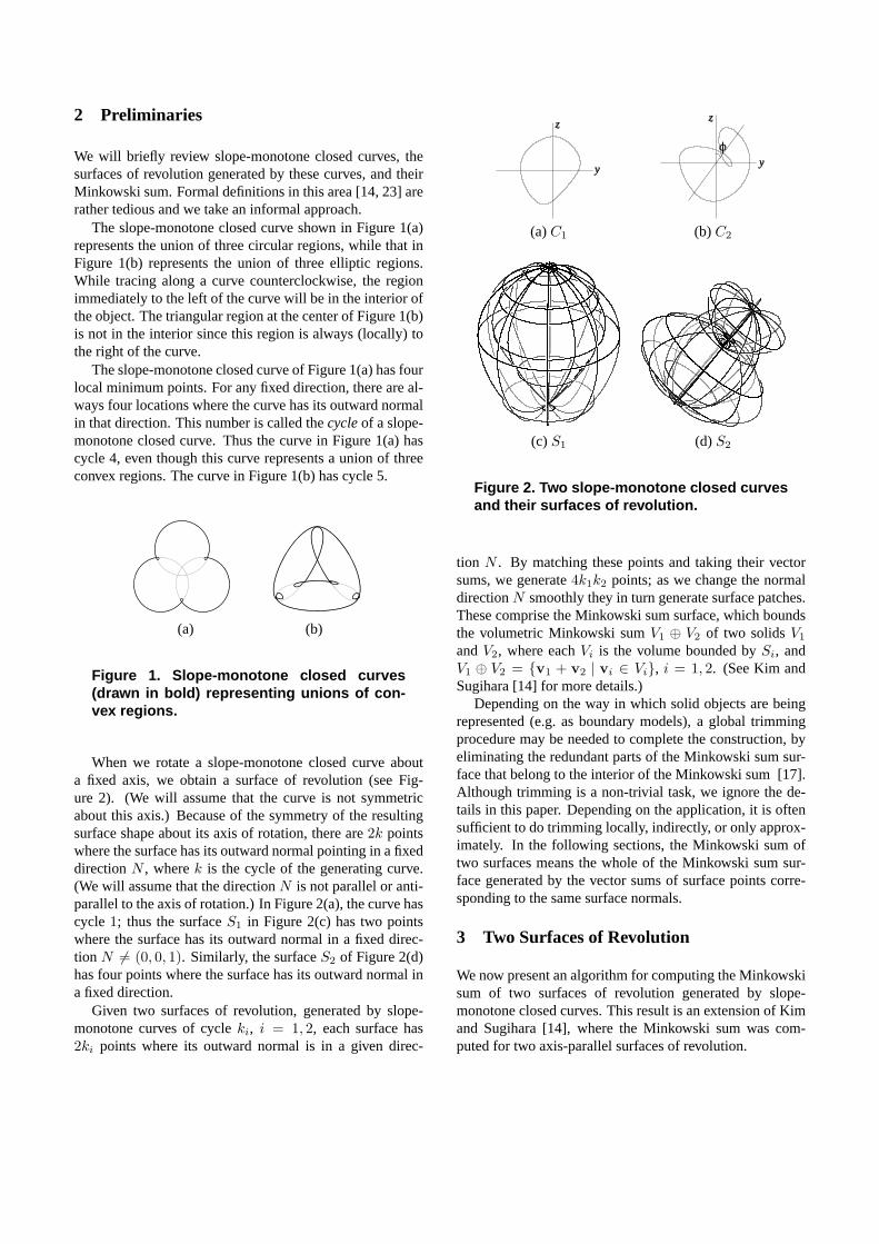
When we rotate a slope-monotone closed curve abouta fixed axis, we obtain a surface of revolution (see Fig-ure 2). (We will assume that the curve is not symmetricabout this axis.) Because of the symmetry of the resultingsurface shape about its axis of rotation, there are2k pointswhere the surface has its outward normal pointing in a fixeddirectionN , wherek is the cycle of the generating curve.(We will assume that the directionN is not parallel or anti-parallel to the axis of rotation.) In Figure 2(a), the curve hascycle 1; thus the surfaceS1 in Figure 2(c) has two pointswhere the surface has its outward normal in a fixed direc-tion N 6= (0, 0, 1). Similarly, the surfaceS2 of Figure 2(d)has four points where the surface has its outward normal ina fixed direction.

Given two surfaces of revolution, generated by slope-monotone curves of cycleki, i = 1, 2, each surface has2ki points where its outward normal is in a given direc-

z

y

z

yϕ

(a)C1 (b) C2

(c) S1 (d) S2

Figure 2. Two slope-monotone closed curvesand their surfaces of revolution.

tion N . By matching these points and taking their vectorsums, we generate4k1k2 points; as we change the normaldirectionN smoothly they in turn generate surface patches.These comprise the Minkowski sum surface, which boundsthe volumetric Minkowski sumV1 ⊕ V2 of two solidsV1

andV2, where eachVi is the volume bounded bySi, andV1 ⊕ V2 = {v1 + v2 | vi ∈ Vi}, i = 1, 2. (See Kim andSugihara [14] for more details.)

Depending on the way in which solid objects are beingrepresented (e.g. as boundary models), a global trimmingprocedure may be needed to complete the construction, byeliminating the redundant parts of the Minkowski sum sur-face that belong to the interior of the Minkowski sum [17].Although trimming is a non-trivial task, we ignore the de-tails in this paper. Depending on the application, it is oftensufficient to do trimming locally, indirectly, or only approx-imately. In the following sections, the Minkowski sum oftwo surfaces means the whole of the Minkowski sum sur-face generated by the vector sums of surface points corre-sponding to the same surface normals.

3 Two Surfaces of Revolution

We now present an algorithm for computing the Minkowskisum of two surfaces of revolution generated by slope-monotone closed curves. This result is an extension of Kimand Sugihara [14], where the Minkowski sum was com-puted for two axis-parallel surfaces of revolution.

3.1 Normal Vectors

Two slope-monotone closed curvesC1 andC2 are definedin theyz-plane as follows:

C1(s) = (0, y1(s), z1(s)), C2(t) = (0, y2(t), z2(t)).

An axis l is contained in theyz-plane and makes an angleϕ with the z-axis. LetS1 denote the surface generated byrotating the curveC1 about thez-axis; and letS2 denoteanother surface generated by rotatingC2 about the axisl:

S1(θ, s) = (−y1(s) sin θ, y1(s) cos θ, z1(s)),S2(ψ, t) = (−y2(t) sin ψ, y2(t) cos ψ cosϕ + z2(t) sin ϕ,

−y2(t) cos ψ sin ϕ + z2(t) cos ϕ),

where

y2(t) = y2(t) cos ϕ− z2(t) sin ϕ,

z2(t) = y2(t) sin ϕ + z2(t) cos ϕ,

for all θ, ψ, s, andt (see Figure 2). Note that the parame-terization ofS2(ψ, t) can be obtained in three steps: (i) ro-tateC2(t) through an angleϕ about thex-axis and call theresulting curveC2(t) = (0, y2(t), z2(t)), (ii) rotate C2(t)through an angleψ about thez-axis, and (iii) rotate the re-sulting surface of revolution through an angle−ϕ about thex-axis.

From the partial derivatives ofS1(θ, s),

∂S1

∂θ= (−y1(s) cos θ,−y1(s) sin θ, 0),

∂S1

∂s= (−y′1(s) sin θ, y′1(s) cos θ, z′1(s)),

we can compute the normal vector ofS1(θ, s) as

∂S1

∂θ× ∂S1

∂s= y1(s)(−z′1(s) sin θ, z′1(s) cos θ,−y′1(s)).

Similarly, from the partial derivatives

∂S2

∂ψ= (−y2(t) cos ψ,−y2(t) sin ψ cosϕ,

y2(t) sin ψ sin ϕ),∂S2

∂t= (−y′2(t) sin ψ, y′2(t) cos ψ cos ϕ + z′2(t) sin ϕ,

−y′2(t) cos ψ sin ϕ + z′2(t) cos ϕ),

we can compute the normal vector ofS2(ψ, t) as

∂S2

∂ψ× ∂S2

∂t=

y2(t)(−z′2(t) sin ψ, z′2(t) cos ψ cosϕ− y′2(t) sin ϕ,

− y′2(t) cos ϕ− z′2(t) cos ψ sin ϕ). (1)

Note that, whenC1(s) passes through thez-axis (andthusy1(s) changes its sign), the normal vector changes itsdirection. Moreover, wheny1(s) = 0, the normal vec-tor vanishes. Thus we define an outward normal vectorN1(θ, s) by deleting the termy1(s), to obtain:

N1(θ, s) = (−z′1(s) sin θ, z′1(s) cos θ,−y′1(s)).

Let N1(θ, s) denote the unit outward normal vector ofS1(θ, s). It can be formulated as:

N1(θ, s) =(−z′1(s) sin θ, z′1(s) cos θ,−y′1(s))√

y′1(s)2 + z′1(s)2.

We can repeat this procedure for the other surfaceS2(ψ, t).In this case the axisl plays a similar role to that of thez-axis in the discussion above, andN2(ψ, t) denotes the unitoutward normal vector ofS2(ψ, t).

3.2 Matching Normal Vectors

To move nearer to computing the Minkowski sum, we nowneed to find all pairs of matching normal vectors ofS1 andS2. That is, givenθ ands, we need to compute the parame-tersψ andt that satisfy the following relation:

N1(θ, s) = N2(ψ, t).

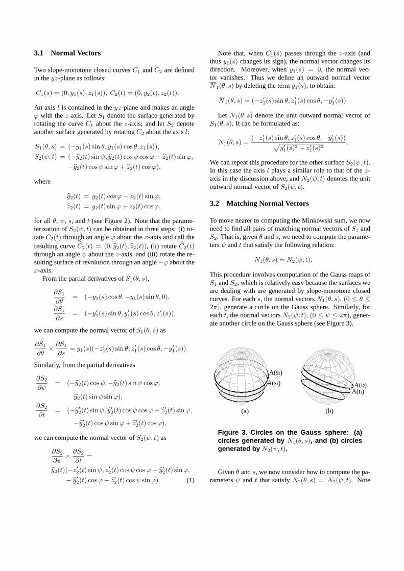
This procedure involves computation of the Gauss maps ofS1 andS2, which is relatively easy because the surfaces weare dealing with are generated by slope-monotone closedcurves. For eachs, the normal vectorsN1(θ, s), (0 ≤ θ ≤2π), generate a circle on the Gauss sphere. Similarly, foreacht, the normal vectorsN2(ψ, t), (0 ≤ ψ ≤ 2π), gener-ate another circle on the Gauss sphere (see Figure 3).

A(s )2

A(s )1 A(t )2A(t )1

(a) (b)

Figure 3. Circles on the Gauss sphere: (a)circles generated by N1(θ, s), and (b) circlesgenerated by N2(ψ, t).

Givenθ ands, we now consider how to compute the pa-rametersψ and t that satisfyN1(θ, s) = N2(ψ, t). Note

N (s)1

N (t)2

N =1 N 2

Figure 4. Matching normal vectors.

thatN2(0, t) is located on theyz-plane, andN2(ψ, t) is ob-tained by rotatingN2(0, t) about the axisl by angleψ. Thuswe have

N2(0, t) = Rl(−ψ)N2(ψ, t)= Rl(−ψ)N1(θ, s), (2)

whereRl(ψ) represents the rotation about axisl by angleψ.

The normal vectorN2(0, t) is computed using Equa-tion (2):

N2(0, t) = Rl(−ψ)N1(θ, s)

=1√

y′1(s)2 + z′1(s)2(3)

−z′1(s)(sin θ cos ψ − cos θ cos ϕ sin ψ)+y′1(s) sin ϕ sin ψ

z′1(s)(sin θ sinψ cosϕ+cos θ cos2 ϕ cos ψ + cos θ sin2 ϕ)+y′1(s)(sin ϕ cos ϕ cos ψ − sinϕ cos ϕ)

−z′1(s) sin θ sinψ sin ϕ−z′1(s) cos θ(sinϕ cosϕ cosψ − cos ϕ sin ϕ)−

y′1(s)(sin2 ϕ cosψ + cos2 ϕ)

.

Since N2(0, t) is contained in theyz-plane, its x-component is equal to zero. Consequently, we have the fol-lowing equation:

−z′1(s)(sin θ cosψ − cos θ cos ϕ sin ψ)+y′1(s) sin ϕ sin ψ = 0,

which produces

tanψ =z′1(s) sin θ

y′1(s) sin ϕ + z′1(s) cos θ cos ϕ. (4)

When cos ψ ≈ 0, we can derivecot ψ instead oftan ψ.Given θ and s, the angleψ = ψ(θ, s) is computed as afunction of θ ands from Equation (4); and we are able tofind the other parametert = t(θ, s) and the curve pointC2(t), using Equation (3). There are two solutions to Equa-tion (4) in the range[0, 2π]: ψa andψb = ψa+π. Moreover,for a fixedψ = ψa or ψ = ψb, there arek2 different val-ues oft that produce the same unit normal vectorN2(ψ, t),wherek2 is the cycle ofC2(t). This means that there are2k2 different pairs(ψ, t) that produce the sameN2(ψ, t),whereψ = ψa or ψ = ψb. A similar argument appliesto N1(θ, s). Consequently, we have4k1k2 pairs of match-ing normal vectors for each normal direction, except thoseparallel or anti-parallel to the rotational axes ofS1 andS2.

3.3 Computing the Minkowski Sum

Let N2(0, ta(θ, s)) be the normal vector computed in Equa-tion (3) using the angleψa(θ, s); and letN2(0, tb(θ, s))be the normal vector computed from the angleψb(θ, s) =ψa(θ, s) + π. Then, from the following normal matchingconditions

N1(θ, s) = N2(ψa(θ, s), ta(θ, s)),N1(θ, s) = N2(ψb(θ, s), tb(θ, s)),

we can define two partial Minkowski sums as follows:

(S1 ⊕ S2)a(θ, s) = S1(θ, s) + S2(ψa(θ, s), ta(θ, s)),(S1 ⊕ S2)b(θ, s) = S1(θ, s) + S2(ψb(θ, s), tb(θ, s)),

for all θ ands. The Minkowski sum ofS1(θ, s) andS2(ψ, t)is then defined as the union of these two surfaces,

(S1 ⊕ S2)(θ, s) = (S1 ⊕ S2)a(θ, s) ∪ (S1 ⊕ S2)b(θ, s),

for all θ ands.Let R(Si), i = 1, 2, denote the three-dimensional vol-

ume which is enclosed by the surfaceSi. When the axes ofrotation are non-parallel, the three-dimensional volumetricMinkowski sum is given as

R(S1)⊕R(S2)= { p1 + p2 | p1 ∈ R(S1), p2 ∈ R(S2)}= R((S1 ⊕ S2)a) ∪R((S1 ⊕ S2)b).

(If the two axes are parallel, there will be some extra vol-umes to consider; see Kim and Sugihara [14] for more de-tails and some examples.) Figure 5 shows two surfaces ofrevolution generated by slope-monotone closed curves. Fig-ure 6 shows their partial Minkowski sums. Figure 7 showstwo tori and their partial Minkowski sums.

(a) (b)

(c) (d)

Figure 5. Two slope-monotone closed curvesand their surfaces of revolution.

(a) (b)

Figure 6. The partial Minkowski sums of twosurfaces of revolution.

4 Two Surfaces of Linear Extrusion

We now move on to consider the Minkowski sum of twosurfaces of linear extrusion, again generated by slope-monotone closed curves. The outward unit normals of asurface of linear extrusion are orthogonal to the directionof extrusion and thus they form a great circle on the Gausssphere. Consequently, the Minkowski sum is relativelyeasy to construct: again, normal matching is done byintersecting the two great circles on the Gauss sphere.

X Y

Z

X Y

Z

(a) (b)

X Y

Z

X Y

Z

(c) (d)

Figure 7. Two tori and their partial Minkowskisums.

4.1 Normal Vectors

Two slope-monotone closed curves are now defined in thexy-plane as:

C1(s) = (x1(s), y1(s), 0), C2(t) = (x2(t), y2(t), 0).

A fixed directionl1 = (a1, 0, c1) is given on thexz-planeand another directionl2 = (a2, b2, c2) is chosen arbitrarily.We define two surfaces of linear extrusion as follows:

S1(u, s) = C1(s) + ul1= (x1(s) + ua1, y1(s), uc1),

S2(v, t) = C2(t) + vl2= (x2(t) + va2, y2(t) + vb2, vc2).

From the partial derivatives ofS1 andS2, which are

∂S1

∂s= (x′1(s), y

′1(s), 0), ∂S1

∂u = (a1, 0, c1),

∂S2

∂t= (x′2(t), y

′2(t), 0), ∂S2

∂v = (a2, b2, c2),

we can compute the unit outward normal vectorsN1 andN2, as follows:

N1(u, s) = N1(u, s)/‖N1(u, s)‖,N2(v, t) = N2(v, t)/‖N2(v, t)‖,

where

N1(u, s) = (c1y′1(s),−c1x

′1(s),−a1y

′1(s)),

N2(v, t) = (c2y′2(t),−c2x

′2(t), b2x

′2(t)− a2y

′2(t)).

Figure 8 shows the images ofN1(u, s) andN2(v, t) whichgenerate great circles on the Gauss sphere. Note that eachcircle is also contained in the plane orthogonal to the extru-sion directionli.

N 1 (u , s)

N 2 (v , t)

l 1

l 2

Figure 8. Gauss images of the surfaces of lin-ear extrusion.

4.2 Matching Normal Vectors

In Figure 8, two great circles intersect at two antipodalpoints. When the extrusion directions are not parallel, thetwo surfaces of linear extrusion have matching normal vec-tors only at the directions±l1×l2. On the other hand, whenthe directions are parallel, the problem essentially reducesto a planar case, which can be solved using the technique ofSugihara et al. [23].

4.3 Computing the Minkowski Sum

Let N± denote two unit normal directions defined as

N± = ± l1 × l2‖l1 × l2‖ .

For the directionN+, there arek1k2 pairs of curve points(C1(si,+), C2(tj,+)) where the surfacesS1 and S2 haveN+ as the unit outward normal vector, fori = 1, . . . , k1,andj = 1, . . . , k2. (Recall thatkl is the cycle of a slope-monotone closed curveCl.) Analogous arguments apply tothe directionN−.

Let N± denote the projection ofN± onto thexy-plane.Then the curveC1(s) hasN+ as its outward normal vectorat eachs = si,+; and similarly the curveC1(s) hasN−as its outward normal vector at eachs = si,−. Analogousarguments apply to the other curveC2(t) and the parameterstj,+ andtj,−.

The Minkowski sum ofS1 and S2 consists of2k1k2

planes, each of which is orthogonal tol1 × l2 and con-tains one of the points:C1(si,+) + C2(tj,+) or C1(si,−) +C2(tj,−), for i = 1, . . . , k1, andj = 1, . . . , k2. Here weconsider surfaces of linear extrusion, which are infinitelyextended. The case of truncated surfaces is more involved;to save space, we omit this more general case.

5 A Surface of Revolution and a Surface ofLinear Extrusion

In this section, we consider the Minkowski sum of a surfaceof revolution and a surface of linear extrusion, where thesurfaces are generated by slope-monotone closed curves.

5.1 Normal Vectors

Two generating curves are defined as follows:

C1(s) = (0, y1(s), z1(s)), C2(t) = (x2(t), y2(t), 0).

Then the surface of revolutionS1 may be parameterized as

S1(θ, s) = (−y1(s) sin θ, y1(s) cos θ, z1(s)),

and the surface of linear extrusionS2 is given as

S2(u, t) = C2(t) + ul = (x2(t) + ua, y2(t) + ub, uc),

wherel = (a, b, c) is a direction vector. Their unit outwardnormal vectors are

N1(θ, s) =(−z′1(s) sin θ, z′1(s) cos θ,−y′1(s))√

y′1(s)2 + z′1(s)2,

N2(u, t) = N2(u, t)/‖N2(u, t)‖,where

N2(u, t) = (cy′2(t), −cx′2(t), bx′2(t)− ay′2(t)).

5.2 Matching Normal Vectors

Givenu andt, we consider how to compute the parametersθ and s so that the two unit normal vectorsN1(θ, s) andN2(u, t) are matched. We can deduce the normal vectorN1(0, s) by rotatingN1(θ, s) through an angle−θ aboutthez-axis. Thus, we have

N1(0, s) = Rz(−θ)N1(θ, s)= Rz(−θ)N2(u, t)= (cy′2(t) cos θ − cx′2(t) sin θ, −cy′2(t) sin θ

−cx′2(t) cos θ, bx′2(t)− ay′2(t)). (5)

Figure 9 shows the Gauss maps of these two sur-faces overlayed on the same Gauss sphere. Since thex-component ofN1(0, s) is equal to zero, we deduce that

tan θ = y′2(t)/x′2(t). (6)

Whencos θ ≈ 0, we can usecot θ instead oftan θ. Givenuandt, the angleθ = θ(u, t) is computed as a function ofuandt from Equation (6); and we are able to find the corre-sponding value ofs = s(u, t) from Equation (5). Note thatthere are2k1k2 pairs of matching normal vectors, excludingthe directions parallel or anti-parallel to the axis of rotationor the direction of extrusion.

l

N 1 (θ, s)

N 2 (u , t)

Figure 9. Two Gauss maps overlayed.

5.3 Computing the Minkowski Sum

The Minkowski sum ofS1(θ, s) andS2(u, t) can be con-structed as a union of partial Minkowski sums. From therelation

N1(θi(u, t), si(u, t)) = N2(u, t), i = 1, ..., 2k1,

we can define partial Minkowski sums as follows:

(S1 ⊕ S2)i(u, t) = S1(θi(u, t), si(u, t)) + S2(u, t),

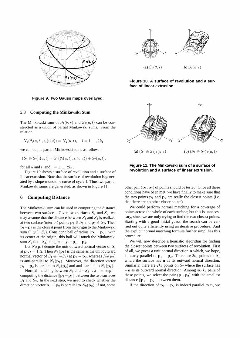
for all u andt, andi = 1, ..., 2k1.Figure 10 shows a surface of revolution and a surface of

linear extrusion. Note that the surface of revolution is gener-ated by a slope-monotone curve of cycle 1. Thus two partialMinkowski sums are generated, as shown in Figure 11.

6 Computing Distance

The Minkowski sum can be used in computing the distancebetween two surfaces. Given two surfacesS1 andS2, wemay assume that the distance betweenS1 andS2 is realizedat two surface (interior) pointsp1 ∈ S1 andp2 ∈ S2. Thenp1−p2 is the closest point from the origin to the MinkowskisumS1⊕ (−S2). Consider a ball of radius‖p1−p2‖, withits center at the origin; this ball will touch the MinkowskisumS1 ⊕ (−S2) tangentially atp1 − p2.

Let Ni(pi) denote the unit outward normal vector ofSi

atpi, i = 1, 2. ThenN1(p1) is the same as the unit outwardnormal vector ofS1 ⊕ (−S2) atp1 − p2, whereasN2(p2)is anti-parallel toN1(p1). Moreover, the direction vectorp1 − p2 is parallel toN2(p2) and anti-parallel toN1(p1).

Normal matching betweenS1 and−S2 is a first step incomputing the distance‖p1−p2‖ between the two surfacesS1 andS2. In the next step, we need to check whether thedirection vectorp1 − p2 is parallel toN2(p2); if not, some

(a)S1(θ, s) (b) S2(u, t)

Figure 10. A surface of revolution and a sur-face of linear extrusion.

(a) (S1 ⊕ S2)1(u, t) (b) (S1 ⊕ S2)2(u, t)

Figure 11. The Minkowski sum of a surface ofrevolution and a surface of linear extrusion.

other pair(p1,p2) of points should be tested. Once all theseconditions have been met, we have finally to make sure thatthe two pointsp1 andp2 are really the closest points (i.e.that there are no other closer points).

We could perform normal matching for a coverage ofpoints across the whole of each surface; but this is unneces-sary, since we are only trying to find the two closest points.Starting with a good initial guess, the search can be car-ried out quite efficiently using an iterative procedure. Andthe explicit normal matching formula further simplifies thisprocedure.

We will now describe a heuristic algorithm for findingthe closest points between two surfaces of revolution. Firstof all, we guess a unit normal directionn which, we hope,is nearly parallel top1 − p2. There are2k1 points onS1

where the surface hasn as its outward normal direction.Similarly, there are2k2 points onS2 where the surface has−n as its outward normal direction. Among4k1k2 pairs ofthese points, we select the pair(p1,p2) with the smallestdistance‖p1 − p2‖ between them.

If the direction ofp1 − p2 is indeed parallel ton, we

are done. Otherwise, we have to modify the normal di-rectionn so as to improve the approximation to the clos-est pointsp1 andp2. The slope-monotonicity of our gen-erating curve greatly simplifies this search procedure. Letp = (p1−p2)/‖p1−p2‖, and consider the Gauss maps ofthe two surfacesS1 and−S2. Figure 12(a) shows a regiondetermined by two pointsn andp on the Gauss sphere ofthe surfaceS1; Figure 12(b) shows a similar region for theother surface−S2. The final solution, wheren andp con-verge, should be located in both regions of the Gauss mapshown in Figures 12(a)–12(b). The intersection of these tworegions is shown in Figure 13, where the intersected regionis bounded by four great circles. In the next iteration, weconsider the great circular arc that connectsn andp on thesphere, and take the location that subdivides this arc in theratio of1 : 2. (We have determined experimentally that thisratio produces a faster convergence than the ‘obvious’ ratioof 1 : 1, which sometimes causes the search to oscillate.)

z

l

n

p

l

z

n

p

(a) (b)

Figure 12. (a) A region in the Gauss map ofS1, and (b) a region in the Gauss map of S2.

z

l

n

p

Figure 13. An intersected region bounded byfour circular arcs.

Using this simple technique to reduce the size of thesearch region at each iteration, we can find a candidate pairof closest points on each surface. To make sure that thisdistance is really the global minimum distance between thetwo surfaces, we can check2k1 points onS1, at which thesurface hasn as its outward normal direction. If there is anypoint among these2k1 that is closer to the other surfaceS2

than the candidatep1, we replacep1 by the point closest toS2. We then repeat the same procedure for the other surfaceS2 using−n andp2. If either p1 or p2 is updated at thisstage, we need to repeat the whole procedure. Otherwise,we have computed the distance betweenS1 andS2.

We have implemented this iterative search algorithm.Figure 14 shows an example where a surface of revolutionmoves around a torus while smoothly changing its orien-tation. The figure shows four ‘snapshots’ of the motion,at each of which the distance between the surfaces wascomputed. This took less than 0.5 msec on average (on a500 MHz Linux machine) using a termination condition of〈n,p〉 > 0.99999. This performance demonstrates the po-tential of this approach in real-time collision detection andavoidance.

Figure 14. An example distance computation.The bold curved line shows the trajectory ofthe center of the moving surface, while boldline segments show the pairs of points real-izing the shortest distances.

7 Conclusions

We have presented an efficient algorithm for constructingthe Minkowski sum of two simple surfaces generated byslope-monotone closed curves. Based on the simple struc-ture of these surfaces, we have formulated explicit equa-tions for matching their surface normals. To demonstratethe effectiveness of this approach, we have implemented analgorithm for computing the distance between two such sur-faces of revolution. Experimental results indicate that ourapproach compares favorably with previous methods. In fu-ture work, we would like to extend the geometrical coverageof our method.

Acknowledgements

The authors would like to thank the anonymous reviewersfor their useful comments. All the algorithms and figurespresented in this paper were implemented and generatedusing the IRIT solid modeling system [4] developed at theTechnion, Israel. This research was supported in part by theKorean Ministry of Information and Communication (MIC)under the program of IT Research Center for CGVR, andin part by the Korean Ministry of Science and Technology(MOST) under the National Research Lab Project.

References

[1] C. Bajaj and M.-S. Kim. Generation of configurationspace obstacles : The case of moving algebraic curves.Algorithmica, 4(2):157–172, 1989.

[2] C. Bajaj and M.-S. Kim. Generation of configurationspace obstacles : The case of moving algebraic sur-faces.The Int’l J. of Robotics Research, 9(1):92–112,1990.

[3] S. Cameron. A comparison of two fast algorithmfor computing the distance between convex polyhedra.IEEE Trans. on Robotics and Automation, 13(6):915–920, 1997.

[4] G. Elber. IRIT 7.0 User’s Manual. TheTechnion-IIT, Haifa, Israel, 1997. Available athttp://www.cs.technion.ac.il/ irit.

[5] P. Ghosh. A mathematical model for shape descriptionusing Minkowski operators.Computer Vision, Graph-ics, and Image Processing, 44(3):239–269, 1988.

[6] P. Ghosh. An algebra of polygons through the notionof negative shapes.Computer Vision, Graphics, andImage Processing: Image Understanding, 54(1):119–144, 1991.

[7] P. Ghosh. A unified computational framework forMinkowski operations. Computers and Graphics,17(4):357–378, 1993.

[8] E. Gilbert and C. Foo. Computing the distance be-tween general convex objects in three-dimensionalspace. IEEE Trans. on Robotics and Automation,6(1):53–61, 1990.

[9] S. Gottschalk, M. Lin and D. Manocha. OBB-Tree: Ahierarchical structure for rapid interference detection,Proc. of ACM SIGGRAPH’96, 171–180, 1996.

[10] L. Guibas, L. Ramshaw, and J. Stolfi. A kinetic frame-work for computer geometry.Proc. of 24th AnnualSymp. on Foundations of Computer Science, 100–111,1983.

[11] P. Jimenez, F. Thomas, and C. Torras. 3D collisiondetection: a survey.Computers & Graphics, 25:269–285, 2001.

[12] A. Kaul and R. Farouki. Computing Minkowski sumsof plane curves.Int’ J. of Computational Geometry &Applications, 5(4):413–432, 1995.

[13] K. Kawachi and H. Suzuki. Distance computation be-tween non-convex polyhedra at short range based ondiscrete Voronoi regions.Proc. of Geometric Model-ing and Processing, Hong Kong, 123–128, 2000.

[14] M.-S. Kim and K. Sugihara. The Minkowski sum oftwo axis-parallel surfaces of revolution generated byslope-monotone closed curves.IEICE Trans. on In-formation and Systems, E84-D(11):1540–1547, 2001.

[15] J.T. Klosowski, M. Held, J.S.B. Mitchell, H. Sowiz-ral, and K. Zikan. Efficient collision detection usingbounding volume hierarchies ofk-DOPs.IEEE Trans.on Visualization and Computer Graphics, 4(1):21–36,1998.

[16] M. Kohler and M. Spreng. Fast computation of theC-space of convex 2D algebraic objects.The Int’ J. ofRobotics Research, 14(6):590–608, 1995.

[17] I.-K. Lee, M.-S. Kim, and G. Elber. Poly-nomial/rational approximation of Minkowski sumboundary curves.Graphical Models and Image Pro-cessing, 60(2):136–165, 1998.

[18] M.C. Lin and J.F. Canny. A fast algorithm for in-cremental distance calculation.Proc. of IEEE Int’lConference on Robotics and Automation, Sacramento,California, 1008–1014, 1991.

[19] M.C. Lin and S. Gottschalk. Collision detection be-tween geometric models: a survey.Mathematics ofSurfaces VIII, R. Cripps, editor, Information Geome-ters, 37–56, 1998.

[20] T. Lozano-Perez and M. A. Wesley. An algorithm forplanning collision free paths among polyhedral obsta-cles.Comm. of the ACM, 22(10):560–570, 1979.

[21] T. Lozano-Perez. Spatial planning : A configura-tion space approach.IEEE Trans. on Computers,32(2):108–120, 1983.

[22] J. Rossignac and A. Kaul. AGRELs and BIPs: Meta-morphosis as a Bezier curve in the space of polyhedra.Computer Graphics Forum, 13(3):C179–C184, 1994.

[23] K. Sugihara, T. Imai, and T. Hataguchi. An algebrafor slope-monotone closed curves.Int’l J. of ShapeModeling, 3(3–4):167–183, 1997.