the modeling and analysis of the word-of-mouth...

Accepted Manuscript

The modeling and analysis of the word-of-mouth marketing

Pengdeng Li, Xiaofan Yang, Lu-Xing Yang, Qingyu Xiong, Yingbo Wu,Yuan Yan Tang

PII: S0378-4371(17)31060-9DOI: https://doi.org/10.1016/j.physa.2017.10.050Reference: PHYSA 18764

To appear in: Physica A

Received date : 29 March 2017Revised date : 6 October 2017

Please cite this article as: P. Li, X. Yang, L.-X. Yang, Q. Xiong, Y. Wu, Y.Y. Tang, The modelingand analysis of the word-of-mouth marketing, Physica A (2017),https://doi.org/10.1016/j.physa.2017.10.050

This is a PDF file of an unedited manuscript that has been accepted for publication. As a service toour customers we are providing this early version of the manuscript. The manuscript will undergocopyediting, typesetting, and review of the resulting proof before it is published in its final form.Please note that during the production process errors may be discovered which could affect thecontent, and all legal disclaimers that apply to the journal pertain.

https://doi.org/10.1016/j.physa.2017.10.050

Highlights of PHYSA-17575

The SIPNS model capturing the WOM marketing processes is established.

The SIPNS model is shown to admit a unique equilibrium.

The impact of different factors on the equilibrium of the model is illuminated.

Experiments suggest that the equilibrium is much likely to be globally attracting.

The influence of different factors on the expected overall profit is ascertained.

*Highlights (for review)

The modeling and analysis of the word-of-mouth marketing

Pengdeng Lia, Xiaofan Yanga,∗, Lu-Xing Yanga,b, Qingyu Xionga, Yingbo Wua, Yuan Yan Tangc

aSchool of Software Engineering, Chongqing University, Chongqing, 400044, ChinabFaculty of Electrical Engineering, Mathematics and Computer Science, Delft University of Technology, Delft, GA 2600, The Netherlands

cDepartment of Computer and Information Science, The University of Macau, Macau

Abstract

As compared to the traditional advertising, word-of-mouth (WOM) communications have striking advantages such assignificantly lower cost and much faster propagation, and this is especially the case with the popularity of online socialnetworks. This paper focuses on the modeling and analysis of the WOM marketing. A dynamic model, known as theSIPNS model, capturing the WOM marketing processes with both positive and negative comments is established. Onthis basis, a measure of the overall profit of a WOM marketing campaign is proposed. The SIPNS model is shown toadmit a unique equilibrium, and the equilibrium is determined. The impact of different factors on the equilibrium of theSIPNS model is illuminated through theoretical analysis. Extensive experimental results suggest that the equilibriumis much likely to be globally attracting. Finally, the influence of different factors on the expected overall profit of aWOM marketing campaign is ascertained both theoretically and experimentally. Thereby, some promotion strategiesare recommended. To our knowledge, this is the first time the WOM marketing is treated in this way.

Keywords: word-of-mouth marketing, overall profit, differential dynamical system, equilibrium, global attractivity

1. Introduction

Promotion is a common form of product sales. The third-party advertising on mass media such as TV and news-paper has long been taken as the major means of promotion. However, this promotion strategy suffers from expensivecost [1, 2]. Furthermore, it has been found that, beyond the early stage of product promotion, the efficacy of advertis-ing diminishes [3]. Word-of-mouth (WOM) communications are a pervasive and intriguing phenomenon. It has beenfound that satisfied and dissatisfied consumers tend to spread positive and negative comments, respectively, regardingthe items they have purchased and used [4, 5]. As compared to positive comments, negative comments are moreemotional and, hence, are more likely to influence the receiver’s opinion. By contrast, positive comments are morecognitive and more considered [6–9]. The significant role of WOM in product sales is supported by broad agreementamong practitioners and academics. Indeed, both positive and negative WOM will affect the purchase decision ofpotential consumers. Due to striking advantages such as significantly lower cost and much faster propagation, theWOM marketing outperforms the traditional advertising marketing [10, 11]. With the increasing popularity of onlinesocial networks such as Facebook, Myspace, and Twitter, the WOM marketing has come to be one of the main formsof product marketing [12].

Currently, the major concern on WOM marketing focuses on finding a set of seeds such that the expected num-ber of individuals activated from this seed set is maximized [13]. Toward this direction, large number of seedingalgorithms have been reported [14–23]. Additionally, a number of dynamic models capturing the WOM spreadingprocesses have been suggested [24–34]. However, all the previous work builds on the premise that a single product ora few competing products are on sale. Typically, customers involved in a marketing campaign may purchase multipleproducts. The ultimate goal of such marketing campaigns is to maximize the overall profit. To achieve the goal, it is

∗Corresponding authorEmail addresses: [email protected] (Pengdeng Li), [email protected] (Xiaofan Yang), [email protected] (Lu-Xing

Yang), [email protected] (Qingyu Xiong), [email protected] (Yingbo Wu), [email protected] (Yuan Yan Tang)

Preprint submitted to Physica A October 6, 2017

*ManuscriptClick here to view linked References

crucial to determine those factors that have significant influence on the overall profit. To our knowledge, so far thereis no literature in this aspect.

This paper addresses the modeling and analysis of the WOM marketing for a consistent set of items. First,a dynamic model, which is known as the SIPNS model, that characterizes the WOM marketing processes with bothpositive and negative comments is established. Second, a measure of the overall profit of a WOM marketing campaignis introduced. Third, the SIPNS model is shown to admit a unique equilibrium, and the equilibrium is figured out.Next, the impact of different factors on the equilibrium of the SIPNS model is expounded through theoretical analysis,and extensive experiments show that the equilibrium is much likely to be globally attracting. Finally, the impact ofdifferent factors on the expected overall profit of a WOM marketing campaign is ascertained through both theoreticalanalysis and simulation experiment. On this basis, some promotion strategies are recommended. To our knowledge,this is the first time the WOM marketing is modeled and analyzed in this way.

The subsequent materials are organized as follows. Section 2 describes the SIPNS model, and presents a measureof the overall profit. Section 3 studies the SIPNS model. Section 4 reveals the influence of different factors on theexpected overall profit. Finally, Section 5 closes this work.

2. The modeling of the WOM marketing

Suppose a marketer is asked to plan a WOM marketing campaign for promoting a batch of items, with the goal ofachieving the maximum possible overall profit. To achieve the goal, the marketer needs to establish a mathematicalmodel for the WOM marketing campaign and, thereby, to make a comparison among different marketing strategies interms of the overall profit. This section is devoted to the modeling of the WOM marketing.

2.1. The target market and its stateLater on, it will be seen that the expected overall profit of a WOM marketing campaign is closely related to the

WOM marketing process. Now, let us establish a dynamic model characterizing the WOM marketing processes.Consider a WOM marketing campaign that starts at time t = 0 and terminates at time t = T . Define the target

market for the campaign at time t as the set of all the consumers and potential consumers involved in the campaign attime t. Let XM(t) denote the size of the target market at time t. Due to the impact of many known or unknown factors,XM(t) is usually uncertain. Let M(t) denote the expectation of XM(t). Then,

M(t) =

∞∑

n=0

n · Pr{XM(t) = n}, t ∈ [0,T ]. (1)

Henceforth, we assume that M(0) = M0.In what follows, it is assumed that, at any time, every individual in the target market is in one of the four possible

states: (a) susceptible, which means that the individual hasn’t recently purchased any item but tends to purchase one,(b) infected, which means that the individual has recently purchased an item but hasn’t yet made any comment on it,(c) positive, which means that the individual has recently purchased an item and has made a positive comment on it,and (d) negative, which means that the individual has recently purchased an item and has made a negative commenton it.

Let XS (t), XI(t), XP(t) and XN(t) denote the number of susceptible, infected, positive and negative individuals attime t, respectively. Then, the vector

X(t) = (XS (t), XI(t), XP(t), XN(t)) (2)

represents the state of the target market at time t. By the relevant definitions, we have

XS (t) + XI(t) + XP(t) + XN(t) = XM(t), t ∈ [0,T ]. (3)

Due to the impact of a variety of factors, these quantities are all uncertain. Let S (t), I(t), P(t) and N(t) denote theexpectation of XS (t), XI(t), XP(t) and XN(t), respectively.

S (t) =

∞∑

n=0

n · Pr{XS (t) = n}, t ∈ [0,T ], (4)

2

I(t) =

∞∑

n=0

n · Pr{XI(t) = n}, t ∈ [0,T ], (5)

P(t) =

∞∑

n=0

n · Pr{XP(t) = n}, t ∈ [0,T ], (6)

N(t) =

∞∑

n=0

n · Pr{XN(t) = n}, t ∈ [0,T ]. (7)

Then, the vectorS(t) = (S (t), I(t), P(t),N(t)) (8)

represents the expected state of the target market at time t.

2.2. A dynamic model capturing the WOM marketing processes

For the purpose of establishing a mathematical model for the WOM marketing processes, let us impose a set ofstatistical hypotheses as follows.

(H1) Due to the influence of advertising, at any time new individuals enter the target market and become susceptibleat the average rate µ > 0. We refer to µ as the entrance rate.

(H2) Due to the loss of interest in shopping, at any time an infected (respectively, a positive, a negative) individualexits from the target market at the average rate δI > 0 (respectively, δP > 0, δN > 0). We refer to δI , δP and δN

as the I-exit rate, P-exit rate, and N-exit rate, respectively. Certainly, we have δP ≤ δI ≤ δN .(H3) Encouraged by the positive comments, at time t a susceptible individual purchases an item and, hence, becomes

infected at the average rate βPP(t), where βP > 0 is a constant. We refer to βP as the P-infection force.(H4) Discouraged by the negative comments, at time t a susceptible individual exits from the market at the average

rate βN N(t), where βN > 0 is a constant. We refer to βN as the N-infection force.(H5) Due to the desire to express the feeling for the recently purchased item, at any time an infected individual makes

a positive (respectively, negative) comment on the item and hence becomes positive (respectively, negative) atthe average rate αP > 0 (respectively, αN > 0). We refer to αP and αN as the P-comment rate and N-commentrate, respectively.

(H6) Due to the shopping desire, an infected (respectively, a positive) individual tends to purchase one more itemand hence becomes susceptible at the average rate γI > 0 (respectively, γP > 0). We refer to γI and γP as theI-viscosity rate and P-viscosity rate, respectively. Certainly, we have γI ≤ γP.

Fig. 1 demonstrates these hypotheses schematically.

( )S t ( )I t

( )P t

( )N t

( )PP tP

N

P

I

( )NN tI

P

N

Figure 1. A schematic representation of the hypotheses (H1)-(H6).

3

This collection of hypotheses implies the following differential dynamical system.

dS (t)dt

= µ − βPP(t)S (t) − βN N(t)S (t) + γPP(t) + γI I(t), t ∈ [0,T ],

dI(t)dt

= βPP(t)S (t) − αPI(t) − αN I(t) − γI I(t) − δI I(t), t ∈ [0,T ],

dP(t)dt

= αPI(t) − γPP(t) − δPP(t), t ∈ [0,T ],

dN(t)dt

= αN I(t) − δN N(t), t ∈ [0,T ],

(9)

subject to M(0) = M0. We refer to the system as the Susceptible-Infected-Positive-Negative-Susceptible model (theSIPNS model, for short). The model captures the expected WOM marketing processes.

2.3. A measure of the overall profit

Based on the SIPNS model, we are ready to measure the overall profit of a WOM marketing campaign. Hereafterwe will take the uniform-profit assumption: selling an item will bring about an one-unit profit.

It can be seen from the second equation in the SIPNS model (9) that the excepted increment of the number ofthe individuals who purchase an item in the infinitesimal time horizon [t, t + dt) is βPP(t)S (t)dt. Hence, the expectedprofit gained in this time horizon is βPP(t)S (t)dt. It follows that the expected overall profit of the marketing campaignis

J = βP

∫ T

0P(t)S (t)dt. (10)

Naturally, we will take this quantity as a measure of the overall profit of the marketing campaign.Obviously, the expected overall profit relies the ten model parameters: the entrance rate, the three exit rates, the

two comment rates, the two infection rates, and the two viscosity rates. So, the expected overall profit can be writtenas

J = J(µ, δI , δP, δN , αP, αN , βP, βN , γI , γP). (11)

3. The dynamics of the SIPNS model

The key to the enhancement of the expected overall profit of a WOM marketing campaign is to gain insight intothe dynamics of the SIPNS model. This section is dedicated to the study of the dynamics of the SIPNS model.

3.1. The equilibrium

An equilibrium of a differential dynamical system is a state of the system such that, starting from the state, thesystem will always stay in the state. Clearly, the equilibria of a differential dynamical system are the best-understoodstates of the system. Therefore, the first step toward understanding the dynamics of a differential dynamical system isto determine all of its equilibria. The following result determines all the equilibria of the SIPNS model (9).

Theorem 1. The SIPNS model (9) admits a unique equilibrium E∗ = (S ∗, I∗, P∗,N∗), where

S ∗ =(αP + αN + γI + δI)(γP + δP)

αPβP,

I∗ =µαPβPδN(γP + δP)

αPβPδN(αN + δI)(γP + δP) + α2PβPδPδN + αNβN(γP + δP)2(αP + αN + γI + δI)

,

P∗ =µα2

PβPδN


,

N∗ =µαPαNβP(γP + δP)


.

(12)

4

Proof. Let E = (S , I, P,N) be an equilibrium of the SIPNS model (9). Then,

µ − βPPS − βN NS + γPP + γI I = 0,βPPS − αPI − αN I − γI I − δI I = 0,

αPI − γPP − δPP = 0,αN I − δN N = 0.

(13)

By the third and fourth equations of the system, we get that

P =αP

γP + δPI, N =

αN

δNI. (14)

Substituting the system into the second equation of the system (13) and noticing that I , 0, we get that S = S ∗.Substituting this equation and the system (14) into the first equation of the system (13) and simplifying, we derive thatI = I∗. Substituting this equation into the system (14), we deduce that P = P∗ and N = N∗. The proof is complete.

It follows from this theorem that, starting from the equilibrium E∗, the SIPNS model will always stay in thisequilibrium. Moreover, the location of the equilibrium is determined.

In reality, however, the probability of the event that a differential dynamical system starts from an equilibrium isoften vanishingly small. To have a full qualitative understanding of the dynamics of the system, one must be aware ofthe evolutionary trend of the system when starting from an initial state other than any of the equilibria, and this ofteninvolves the stability properties of the equilibrium. An equilibrium is stable if, starting from near the equilibrium, thesystem will always stay near the equilibrium. An equilibrium is globally attracting if, starting from any initial state,the system approaches the equilibrium. An equilibrium is globally stable if it is stable and globally attracting.

Because of the inherent complexity of the SIPNS model, we failed to prove the stability of its equilibrium, letalone the global stability of the equilibrium. Nevertheless, due to its practical significance and potential application,the SIPNS model is worth further study. Next, let us turn our attention to the study of the SIPNS model throughcomputer simulations, with emphasis on the impact of different factors on the dynamics of the model.

All the subsequent theorems are proved either through direct observation or by applying the following lemma.

Lemma 1. Let a, b, c, d > 0. The following claims hold.

(a) The function f1(x) = ax + bx (x > 0) is strictly decreasing with x <

√ba , is strictly increasing with x >

√ba , and

attains the minimum at x =

√ba .

(b) The function f2(x) = ax+bcx+d (x > 0) is strictly increasing or strictly decreasing or constant according as ad > bc

or ad < bc or ad = bc.

Proof. The first claim follows from f ′1(x) = a − bx2 . The second claim follows from f ′2(x) = ad−bc

(cx+d)2 .

3.2. The impact of the entrance rate

By Theorem 1, the entrance rate affects the equilibrium of the SIPNS model in the following way.

Theorem 2. Consider the equilibrium E∗ = (S ∗, I∗, P∗,N∗) of the SIPNS model (9). The following claims hold.

(a) S ∗ is irrelevant to µ.(b) I∗, P∗ and N∗ are strictly incresing with µ.

Extensive experiments show that, typically, the entrance rate affects the dynamics of the SIPNS model in the wayshown in Fig. 2. In general, it is drawn that, for any entrance rate, the SIPNS model approaches the equilibrium.

5

5

4

3

2

1

0

S(t)

200150100500

Time

(a)5

4

3

2

1

0

I(t)

4003002001000

Time

(b)

1.0

0.8

0.6

0.4

0.2

0.0

P(t)

4003002001000

Time

(c)100x10

-3

80

60

40

20

0

N(t

)

4003002001000

Time

(d)

Figure 2. The time plots of S (t), I(t), P(t) and N(t) for different entrance rates.

3.3. The impact of the three exit rates

By Theorem 1, the I-exit rate affects the equilibrium of the SIPNS model in the following way.


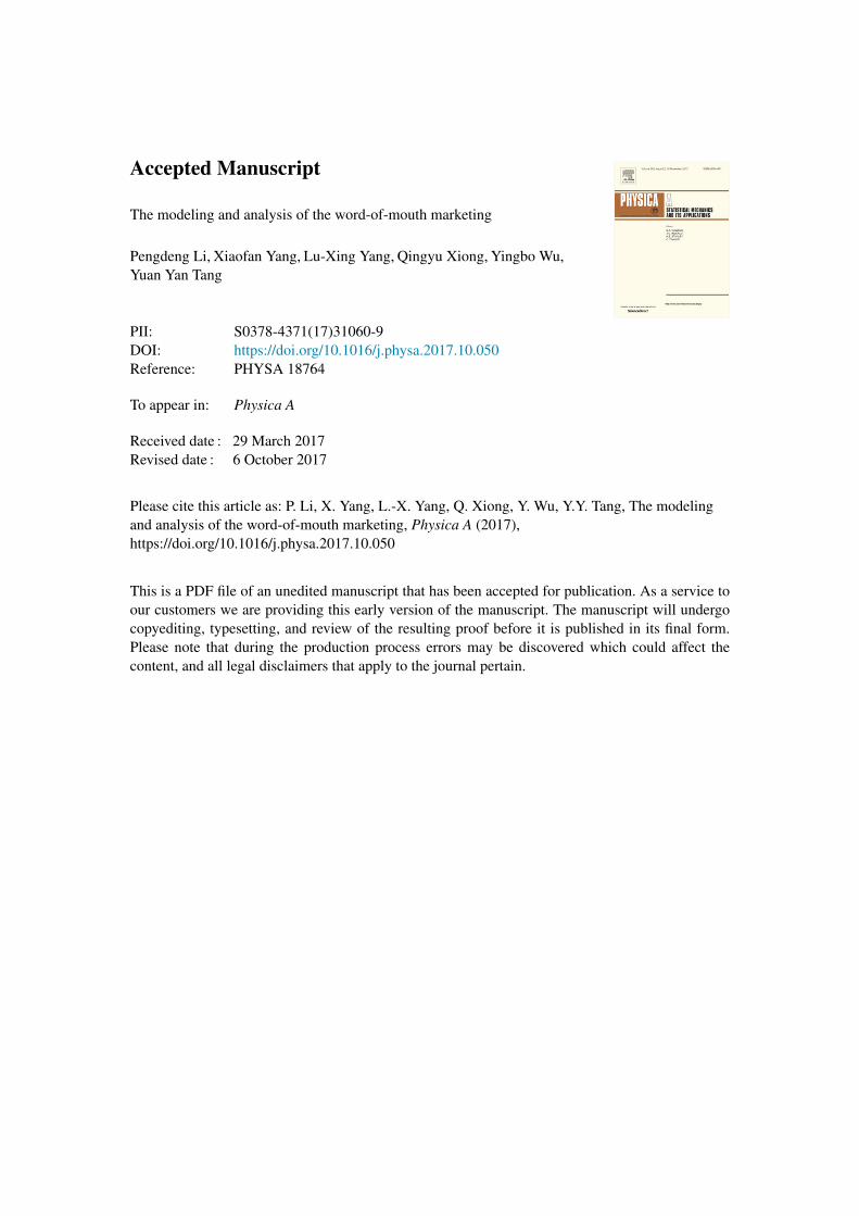
(a) S ∗ is strictly increasing with δI .(b) I∗, P∗ and N∗ are strictly decreasing with δI .

Extensive experiments show that, typically, the I-exit rate affects the dynamics of the SIPNS model in the wayshown in Fig. 3. In general, it is drawn that, for any I-exit rate, the SIPNS model approaches the equilibrium.

Let

δ∗P = αP

√βPδPδN

αNβN(αP + αN + γI + δI)− γP. (15)

By Theorem 1, the P-exit rate affects the equilibrium of the SIPNS model in the following way.


(a) S ∗ is strictly increasing with δP.(b) P∗ is strictly decreasing with δP.(c) If δ∗P ≤ 0, then I∗ and N∗ are strictly decreasing with δP.(d) If δ∗P > 0, then I∗ and N∗ are strictly increasing with δP < δ∗P, are strictly decreasing with δP > δ∗P, and attain

their respective maximum at δP = δ∗P.

Extensive experiments show that, typically, the P-exit rate affects the dynamics of the SIPNS model in the wayshown in Fig. 4. In general, it is drawn that, for any P-exit rate, the SIPNS model approaches the equilibrium.

By Theorem 1, the N-exit rate affects the equilibrium of the SIPNS model in the following way.


6

14

12

10

8

6

4

2

0

S(t)

200150100500

Time

(a)5

4

3

2

1

0

I(t)

200150100500

Time

(b)

0.35

0.30

0.25

0.20

0.15

0.10

0.05

0.00

P(t)

200150100500

Time

(c)0.30

0.25

0.20

0.15

0.10

0.05

0.00

N(t

)

200150100500

Time

(d)

Figure 3. The time plots of S (t), I(t), P(t) and N(t) for different I-exit rates.

(a) S ∗ is irrelevant to δN .(b) I∗ and P∗ are strictly increasing with δN .(c) N∗ is strictly decreasing with δN .

Extensive experiments show that, typically, the N-exit rate affects the dynamics of the SIPNS model in the wayshown in Fig. 5. In general, it is drawn that, for any N-exit rate, the SIPNS model approaches the equilibrium.

3.4. The impact of the two comment ratesLet

α∗P = (γP + δP)

√αNβN(αN + γI + δI)

βPδPδN. (16)

By Theorem 1, the P-comment rate affects the equilibrium of the SIPNS model in the following way.


(a) S ∗ is strictly decreasing with αP.(b) P∗ is strictly increasing with αP.(c) I∗ and N∗ are strictly increasing with αP < α

∗P, are strictly decreasing with αP > α

∗P, and attain their respective

maximum at αP = α∗P.

Extensive experiments show that, typically, the P-comment rate affects the dynamics of the SIPNS model inthe way shown in Fig. 6. In general, it is drawn that, for any P-comment rate, the SIPNS model approaches theequilibrium.

Let

α∗N =1

γP + δP

√αPβPδIδN(γP + δP) + α2

PβPδPδN

βN. (17)

By Theorem 1, the N-comment rate affects the equilibrium of the SIPNS model in the following way.

7

16

12

8

4

0

S(t)

200150100500

Time

(a)5

4

3

2

1

0

I(t)

200150100500

Time

(b)

0.30

0.25

0.20

0.15

0.10

0.05

0.00

P(t)

200150100500

Time

(c)0.4

0.3

0.2

0.1

0.0

N(t

)

200150100500

Time

(d)

Figure 4. The time plots of S (t), I(t), P(t), and N(t) for different P-exit rates.


(a) S ∗ is strictly increasing with αN .(b) I∗ and P∗ are strictly decreasing with αN .(c) N∗ is strictly increasing with αN < α∗N , is strictly decreasing with α∗N , and attains the maximum at αN = α∗N .

Extensive experiments show that, typically, the N-comment rate affects the dynamics of the SIPNS model inthe way shown in Fig. 7. In general, it is drawn that, for any N-comment rate, the SIPNS model approaches theequilibrium.

3.5. The impact of the two infection forcesBy Theorem 1, the P-infection rate affects the equilibrium of the SIPNS model in the following way.


(a) S ∗ is strictly decreasing with βP.(b) I∗, P∗ and N∗ are strictly increasing with βP.

Extensive experiments show that, typically, the P-infection force affects the dynamics of the SIPNS model inthe way shown in Fig. 8. In general, it is drawn that, for any P-infection force, the SIPNS model approaches theequilibrium.

By Theorem 1, the N-infection rate affects the equilibrium of the SIPNS model in the following way.


(a) S ∗ is irrelevant to βN .(b) I∗, P∗ and N∗ are strictly decreasing with βN .

Extensive experiments show that, typically, the N-infection force affects the dynamics of the SIPNS model inthe way shown in Fig. 9. In general, it is drawn that, for any N-infection force, the SIPNS model approaches theequilibrium.

8

3.5

3.0

2.5

2.0

1.5

1.0

0.5

0.0

S(t)

100806040200

Time

(a)

5

4

3

2

1

0

I(t)

100806040200

Time

(b)

1.2

1.0

0.8

0.6

0.4

0.2

0.0

P(t)

100806040200

Time

(c)1.2

1.0

0.8

0.6

0.4

0.2

0.0

N(t

)

100806040200

Time

(d)

Figure 5. The time plots of S (t), I(t), P(t), and N(t) for different N-exit rates.

3.6. The impact of the two viscosity ratesBy Theorem 1, the I-viscosity rate affects the equilibrium of the SIPNS model in the following way.


(a) S ∗ is strictly increasing with γI .(b) I∗, P∗ and N∗ are strictly decreasing with γI .

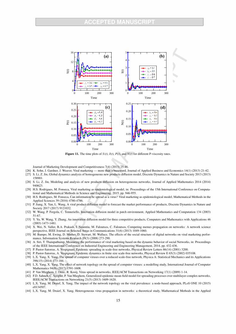
Extensive experiments show that, typically, the I-viscosity rate affects the dynamics of the SIPNS model in the wayshown in Fig. 10. In general, it is drawn that, for any I-viscosity rate, the SIPNS model approaches the equilibrium.

By Theorem 1, the P-viscosity rate affects the equilibrium of the SIPNS model in the following way.Let

γ∗P = αP

√βPδPδN

αNβN(αP + αN + γI + δI)− δP. (18)


(a) S ∗ is strictly increasing with γP.(b) P∗ is strictly decreasing with γP.(c) If γ∗P ≤ 0, then I∗ and N∗ are strictly decreasing with γP.(d) If γ∗P > 0, then I∗ and N∗ are strictly increasing with γP < γ∗P, are strictly decreasing with γP > γ∗P, and attain

their respective maximum at γP = γ∗P.

Extensive experiments show that, typically, the P-viscosity rate affects the dynamics of the SIPNS model in theway shown in Fig. 11. In general, it is drawn that, for any P-viscosity rate, the SIPNS model approaches the equilib-rium.

Combining the above discussions, we propose the following conjecture.

Conjecture 1. The equilibrium of the SIPNS model (9) is globally attracting. That is, starting from any initial state,the model approaches the equilibrium.

9

12

10

8

6

4

2

0

S(t)

200150100500

Time

(a)5

4

3

2

1

0

I(t)

200150100500

Time

(b)

1.4

1.2

1.0

0.8

0.6

0.4

0.2

0.0

P(t)

200150100500

Time

(c)

0.30

0.25

0.20

0.15

0.10

0.05

0.00

N(t

)

200150100500

Time

(d)

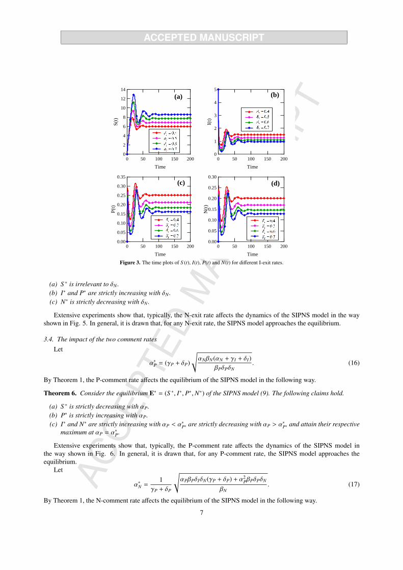
Figure 6. The time plots of S (t), I(t), P(t), and N(t) for different P-comment rates.

4. The expected overall profit of a WOM marketing campaign

This section is dedicated to the study of the impact of different factors on the expected overall profit of a WOMmarketing campaign. First, it should be noted that, when T is large enough, the expected overall profit can be approx-imated by the following quantity.

J∗ = βPT P∗S ∗ = TµαPβPδN(αP + αN + γI + δI)(γP + δP)


. (19)

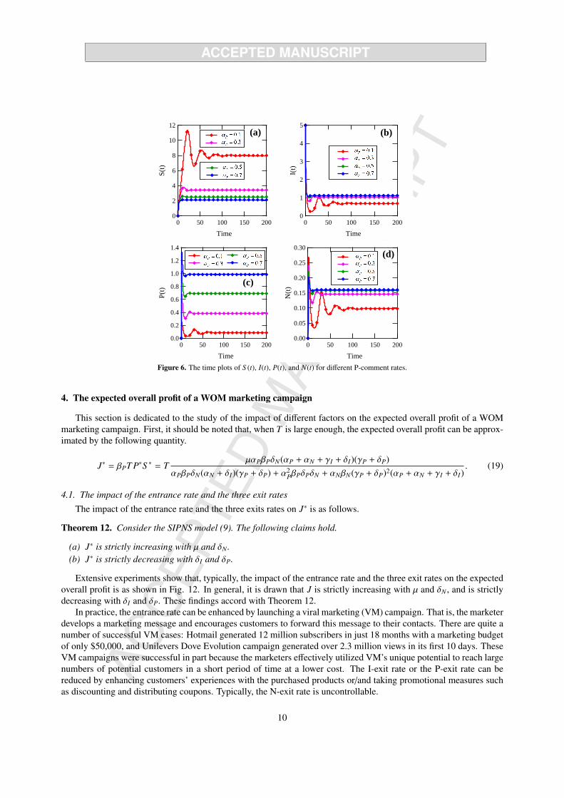
4.1. The impact of the entrance rate and the three exit rates

The impact of the entrance rate and the three exits rates on J∗ is as follows.

Theorem 12. Consider the SIPNS model (9). The following claims hold.

(a) J∗ is strictly increasing with µ and δN .(b) J∗ is strictly decreasing with δI and δP.

Extensive experiments show that, typically, the impact of the entrance rate and the three exit rates on the expectedoverall profit is as shown in Fig. 12. In general, it is drawn that J is strictly increasing with µ and δN , and is strictlydecreasing with δI and δP. These findings accord with Theorem 12.

In practice, the entrance rate can be enhanced by launching a viral marketing (VM) campaign. That is, the marketerdevelops a marketing message and encourages customers to forward this message to their contacts. There are quite anumber of successful VM cases: Hotmail generated 12 million subscribers in just 18 months with a marketing budgetof only $50,000, and Unilevers Dove Evolution campaign generated over 2.3 million views in its first 10 days. TheseVM campaigns were successful in part because the marketers effectively utilized VM’s unique potential to reach largenumbers of potential customers in a short period of time at a lower cost. The I-exit rate or the P-exit rate can bereduced by enhancing customers’ experiences with the purchased products or/and taking promotional measures suchas discounting and distributing coupons. Typically, the N-exit rate is uncontrollable.

10

6

5

4

3

2

1

0

S(t)

200150100500

Time

(a)5

4

3

2

1

0

I(t)

200150100500

Time

(b)

1.2

1.0

0.8

0.6

0.4

0.2

0.0

P(t)

200150100500

Time

(c)1.2

1.0

0.8

0.6

0.4

0.2

0.0

N(t

)

200150100500

Time

(d)

Figure 7. The time plots of S (t), I(t), P(t) and N(t) for different N-comment rates.

4.2. The impact of the two comment rates

The impact of the two comment rates on J∗ is as follows.


(a) J∗ is strictly increasing with αP.(b) J∗ is strictly decreasing with αN .

Extensive experiments show that, typically, the impact of the two comment rates on the expected overall profit isas shown in Fig. 13. In general, it is drawn that J is strictly increasing with αP, and is strictly decreasing with αN .These findings conform to Theorem 13.

In practice, the P-comment rate can be enhanced, and the N-comment rate can be reduced, by enhancing cus-tomers’ experiences.

4.3. The impact of the two infection forces

The impact of the two infection forces on J∗ is as follows.


(a) J∗ is strictly increasing with βP.(b) J∗ is strictly decreasing with βN .

Extensive experiments show that, typically, the impact of the two infection forces on the expected overall profitis as shown in Fig. 14. In general, it is drawn that J is strictly increasing with βP, and is strictly decreasing with βN .These findings agree with Theorem 14. In practice, the P-infection force can be enhanced by enhancing customers’experiences and, hence, earning positive WOM. The N-infection force is often uncontrollable.

11

25

20

15

10

5

0

S(t)

4003002001000

Time

(a)5

4

3

2

1

0

I(t)

4003002001000

Time

(b)

1.4

1.2

1.0

0.8

0.6

0.4

0.2

0.0

P(t)

4003002001000

Time

(c)0.25

0.20

0.15

0.10

0.05

0.00

N(t

)

4003002001000

Time

(d)

Figure 8. The time plots of S (t), I(t), P(t) and N(t) under different P-infection forces.

4.4. The impact of the two viscosity rates

See Eq. (18). The impact of the two viscosity rates on J∗ is as follows.


(a) J∗ is strictly increasing with γI .(b) If γ∗P ≤ 0, then J∗ is strictly decreasing with γP.(c) If γ∗P > 0, then J∗ is strictly increasing with γP < γ∗P, is strictly decreasing with γP > γ∗P, and attains the

maximum at γP = γ∗P.

Extensive experiments show that, typically, the impact of the two viscosity rates on the expected overall profit isas shown in Fig. 15. In general, the following conclusions are drawn.

(a) J is increasing with γI .(b) There is γ∗∗P (T ) (T > 0) such that (1) γ∗∗P (T )→ γ∗P as T → ∞, (2) if γ∗∗P (T ) ≤ 0, then J is strictly decreasing with

γP, and (3) if γ∗∗P (T ) > 0, then J is strictly increasing with γP < γ∗∗P (T ), is strictly decreasing with γP > γ

∗∗P (T ),

and attains the maximum at γP = γ∗∗P (T ).

These findings comply with Theorem 15.In practice, the I-viscosity rate can be enhanced by enhancing customers’ experiences or by taking promotional

measures.

5. Conclusions and remarks

WOM marketing processes with both positive and negative comments have been modeled as the SIPNS model,and a measure of the overall profit of WOM marketing campaigns has been proposed. The SIPNS model has beenshown to admit a unique equilibrium, and the impact of different factors on the equilibrium has been determined.Furthermore, extensive experiments have shown that the equilibrium is much likely to be globally attracting. Finally,

12

25

20

15

10

5

0

S(t)

3002001000

Time

(a)5

4

3

2

1

0

I(t)

3002001000

Time

(b)

2.5

2.0

1.5

1.0

0.5

0.0

P(t)

3002001000

Time

(c)0.4

0.3

0.2

0.1

0.0

N(t

)

3002001000

Time

(d)

Figure 9. The time plots of S (t), I(t), P(t) and N(t) under different N-infection forces.

the influence of different factors on the expected overall profit has been ascertained. On this basis, some promotionstrategies have been suggested.

Toward this direction, lots of efforts are yet to be made. It is well known that the structure of the WOM networkhas significant influence on the performance of a viral marketing [35, 36]. The proposed SIPNS model is a population-level model and hence does not allow the analysis of this influence. To reveal the impact of the WOM network onthe performance, network-level spreading models [37–40] or individual-level spreading models [41–47] are betteroptions. The profit model presented in this paper builds on the uniform-profit assumption. However, in everyday lifedifferent products may have separate profits. Hence, it is of practical importance to construct a non-uniform profitmodel. Also, a customer may purchase multiple items a time, and the corresponding model is yet to be developed.Typically, WOM marketing campaigns are subject to limited budgets. The dynamic optimal control strategy againstmalicious epidemics [48–52] may be borrowed to the analysis of WOM marketing so as to achieve the maximumpossible net profit.

Acknowledgments

The authors are grateful to the anonymous reviewers and the editor for their valuable comments and suggestions.This work is supported by Natural Science Foundation of China (Grant No. 61572006), National Sci-Tech SupportProgram of China (Grant No. 2015BAF05B03), and Fundamental Research Funds for the Central Universities (GrantNo. 106112014CDJZR008823).

References

[1] G. Armstrong, P. Kotler, Marketing: An introduction (11th Edition), Prentice Hall, 2012.[2] D. Grewal, M. Levy, Marketing (5th Edition), McGraw-Hill Education, 2016.[3] J. Goldenberg, B. Libai, E. Muller, Talk of the network: A complex systems look at the underlying process of word-of-mouth, Marketing

Letters 12(3) (2001) 211-223.[4] V. Mahajan, E. Muller, R.A. Kerin, Introduction strategy for new products with positive and negative word-of-mouth, Management Science

30(12) (1984) 1389-1404.

13

20

15

10

5

0

S(t)

3002001000

Time

(a)5

4

3

2

1

0

I(t)

3002001000

Time

(b)

0.25

0.20

0.15

0.10

0.05

0.00

P(t)

3002001000

Time

(c)0.30

0.25

0.20

0.15

0.10

0.05

0.00

N(t

)

3002001000

Time

(d)

Figure 10. The time plots of S (t), I(t), P(t), and N(t) for different I-viscosity rates.

[5] E. Anderson, Customer satisfaction and word-of-mouth, Journal of Service Research 1(1) (1998) 5-17.[6] P.M. Herr, F.R. Kardes, J. Kim, Effects of word-of-mouth and product attribute information on persuasion: An accessibility-diagnosticity

perspective, Journal of Consumer Research 17 (1991) 454-462.[7] D. Charlett, R. Garland, N. Marr, How damaging is negative word of mouth? Marketing Bulletin 6 (1995) 42-50.[8] J.C. Sweeney, G.N. Soutar, T. Mazzarol, The differences between positive and negative word-of-mouth: Emotion as a differentiator? S.

Gopalan, N. Taher (eds), Viral Marketing: Concepts and Cases, Icfai University Press, 2007, pp. 156-168.[9] N. Ahmad, J. Vveinhardt, R.R. Ahmed, Impact of word of mouth on consumer buying decision, European Journal of Business and Manage-

ment 6(31) (2014) 394-403.[10] I.R. Misner, The World’s Best Known Marketing Secret: Building Your Business with Word-of-Mouth Marketing (2nd Edition), Bard Press,

1999.[11] J. Chevalier, M. Dina, The effect of word of mouth on sales: online book reviews, Journal of Marketing Research 43 (2006) 345-354.[12] M. Trusov, R.E. Bucklin, K. Pauwels, Effects of word-of-mouth versus traditional marketing: Findings from an Internet social networking

sites, Journal of Marketing 73(5) (2009) 90-102.[13] R. Peres, E. Muller, V. Mahajan, Innovation diffusion and new product growth models: A critical review and research directions, International

Journal of Research in Marketing 27 (2010) 91-106.[14] D. Kempe, J. Kleinberg, E, Tardos, Influential nodes in a diffusion model for social networks, in: Proceedings of the 32nd International

Conference on Automata, Languages and Programming, 2005, pp. 1127-1138.[15] W. Chen, Y. Wang, S. Yang, Efficient influence maximization in social networks, in: Proceedings of the 15th ACM SIGKDD International

Conference on Knowledge Discovery and Data Mining, 2009, pp. 199-208.[16] O. Hinz, B. Skiera, C. Barrot, J.U. Becker, Seeding strategies for viral marketing: An empirical comparison, Journal of Marketing 75 (2011)

55-71.[17] T.N. Dinh, H. Zhang, D.T. Nguyen, M.T. Thai, Cost-effective viral marketing for time-critical campaigns in large-scale social networks,

IEEE/ACM Transactions on Networking 22(6) (2014) 2001-2011.[18] A. Mochalova, A. Nanopoulos, A targeted approach to viral marketing, Electronic Commerce Research and Applications 13 (2014) 283-294.[19] D. Kempe, J. Kleinberg, E, Tardos, Maximizing the spread of influence through a social network, Theory of Computing 11(4) (2015) 105-147.[20] M. Samadi, A. Nikolaev, R. Nagi, A subjective evidence model for influence maximization in social networks, Omega 59(B) (2016) 263-278.[21] H. Zhang, D.T. Nguyen, S. Das, H. Zhang, M.T. Thai, Least cost influence maximization across multiple social networks, IEEE/ACM

Transactions on Networking 24(2) (2016) 929-939.[22] S. Bharathi, D. Kempe, M. Salek, Competitive influence maximization in social networks, X. Deng, F. C. Graham (eds) International Work-

shop on Web and Internet Economics, Internet and Network Economics, Lecture Notes in Computer Science, vol. 4858, 2007, pp. 306-311.[23] H. Zhang, H. Zhang, A. Kuhnle, M.T. Thai, Profit maximization for multiple products in online social networks, in: Proceedings of the IEEE

International Conference on Computer Communications, 2016, pp. 1-9.[24] F.M. Bass, A new product growth for model consumer durables, Management Science 15(5) (1969) 215-227.[25] J.T. Gardner, K. Sohn, J.Y. Seo, J.L. Weaver, Analysis of an epidemiological model of viral marketing: when viral marketing efforts fall flat,

14

16

12

8

4

0

S(t)

3002001000

Time

(a)5

4

3

2

1

0

I(t)

3002001000

Time

(b)

0.30

0.25

0.20

0.15

0.10

0.05

0.00

P(t)

3002001000

Time

(c)0.25

0.20

0.15

0.10

0.05

0.00

N(t

)

3002001000

Time

(d)

Figure 11. The time plots of S (t), I(t), P(t), and N(t) for different P-viscosity rates.

Journal of Marketing Development and Competitiveness 7(4) (2013) 25-46.[26] K. Sohn, J. Gardner, J. Weaver, Viral marketing — more than a buzzword, Journal of Applied Business and Economics 14(1) (2013) 21-42.[27] S. Li, Z. Jin, Global dynamics analysis of homogeneous new products diffusion model, Discrete Dynamics in Nature and Society 2013 (2013)

158901.[28] S. Li, Z. Jin, Modeling and analysis of new products diffusion on heterogeneous networks, Journal of Applied Mathematics 2014 (2014)

940623.[29] H.S. Rodrigues, M. Fonseca, Viral marketing as epidemiological model, in: Proceedings of the 15th International Conference on Computa-

tional and Mathematical Methods in Science and Engineering, 2015, pp. 946-955.[30] H.S. Rodrigues, M. Fonseca, Can information be spread as a virus? Viral marketing as epidemiological model, Mathematical Methods in the

Applied Sciences 39 (2016) 4780-4786.[31] P. Jiang, X. Yan, L. Wang, A viral product diffusion model to forecast the market performance of products, Discrete Dynamics in Nature and

Society 2017 (2017) 9121032.[32] W. Wang, P. Fergola, C. Tenneriello, Innovation diffusion model in patch environment, Applied Mathematics and Computation 134 (2003)

51-67.[33] Y. Yu, W. Wang, Y. Zhang, An innovation diffusion model for three competitive products, Computers and Mathematics with Applications 46

(2003) 1473-1481.[34] X. Wei, N. Valler, B.A. Prakash, I. Neamtiu, M. Faloutsos, C. Faloutsos, Competing memes propagation on networks: A network science

perspective, IEEE Journal on Selected Areas in Communications 31(6) (2013) 1049-1060.[35] M. Bampo, M. Ewing, D. Mather, D. Stewart, M. Wallace, The effects of the social structure of digital networks on viral marketing perfor-

mance, Information Systems Research 19(3) (2008) 273-290.[36] A. Siri, T. Thaiupathump, Measuring the performance of viral marketing based on the dynamic behavior of social Networks, in: Proceedings

of the IEEE International Conference on Industrial Engineering and Engineering Management, 2014, pp. 432-436.[37] P. Pastor-Satorras, A. Vespignani, Epidemic spreading in scale-free networks, Physical Review Letters 86(14) (2001) 3200.[38] P. Pastor-Satorras, A. Vespignani, Epidemic dynamics in finite size scale-free networks, Physical Review E 65(3) (2002) 035108.[39] L.X. Yang, X. Yang, The spread of computer viruses over a reduced scale-free network, Physica A: Statistical Mechanics and its Applications

396(15) (2014) 173-184.[40] L.X. Yang, X. Yang, The effect of network topology on the spread of computer viruses: a modelling study, International Journal of Computer

Mathematics 94(8) (2017) 1591-1608.[41] P. Van Mieghem, J. Omic, R. Kooij, Virus spread in networks, IEEE/ACM Transactions on Networking 17(1) (2009) 1-14.[42] F.D. Sahneh, C. Scoglio, P. Van Mieghem, Generalized epidemic mean-field model for spreading processes over multilayer complex networks,

IEEE/ACM Transactions on Networking 21(5) (2013) 1609-1620.[43] L.X. Yang, M. Draief, X. Yang, The impact of the network topology on the viral prevalence: a node-based approach, PLoS ONE 10 (2015)

e0134507.[44] L.X. Yang, M. Draief, X. Yang, Heterogeneous virus propagation in networks: a theoretical study, Mathematical Methods in the Applied

15

3500

3000

2500

2000

1500

1000

500

0

Exp

ecte

d ov

eral

l pro

fit

1.00.80.60.40.20.0

(a)

450

400

350

300

250

200

150

Exp

ecte

d ov

eral

l pro

fit

0.80.60.40.20.0

(b)

280

260

240

220

200

180

160

140

Exp

ecte

d ov

eral

l pro

fit

0.400.300.200.100.00

(c)

240

236

232

228

224

Exp

ecte

d ov

eral

l pro

fit

1.00.90.80.70.60.5

(d)

Figure 12. The expected overall profit versus (a) the entrance rate, (b) the I-exit rate, (c) the P-exit rate, and (d) the N-exit rate.

250

200

150

100

50

0

Exp

ecte

d ov

eral

l pro

fit

1.00.80.60.40.20.0

(a)

300

250

200

150

100

50

0

Exp

ecte

d ov

eral

l pro

fit

1.00.80.60.40.20.0

(b)

Figure 13. The expected overall profit versus (a) the P-comment rate, and (b) the N-comment rate.

Sciences 40(5) (2017) 1396-1413.[45] L.X. Yang, X. Yang, Y. Wu, The impact of patch forwarding on the prevalence of computer virus: A theoretical assessment approach, Applied

Mathematical Modelling 43 (2017) 110-125.[46] L.X. Yang, X. Yang, Y.Y. Tang, A bi-virus competing spreading model with generic infection rates, IEEE Transactions on Network Science

and Engineering, doi: 10.1109/TNSE.2017.2734075.[47] L.X. Yang, P. Li, X. Yang, Y.Y. Tang, Security evaluation of the cyber networks under advanced persistent threats, IEEE Access, doi:

10.1109/ACCESS.2017.2757944.[48] V.M. Preciado, M. Zargham, C. Enyioha, A. Jadbabaie, G. Pappas, Optimal resource allocation for network protection against spreading

processes, IEEE Transactions on Control of Network Systems 1(1) (2014) 99-108.[49] H. Shakeri, F.D. Sahneh, C. Scoglio, Optimal information dissemination strategy to promote preventive behaviours in multilayer networks,

Mathematical Bioscience and Engineering 12(3) (2015) 609-623.[50] L.X. Yang, M. Draief, X. Yang, The optimal dynamic immunization under a controlled heterogeneous node-based SIRS model, Physica A:

Statistical Mechanics and its Applications 450 (2016) 403-415.[51] C. Nowzari, V.M. Preciado, G.J. Pappas, Analysis and control of epidemics: A survey of spreading processes on complex networks, IEEE

Control Systems 36(1) (2016) 26-46.[52] T.R. Zhang, L.X. Yang, X. Yang, Y. Wu, Y.Y. Tang, The dynamic malware containment under a node-level epidemic model with the alert

compartment, Physica A: Statistical Mechanics and its Applications 470 (2017) 249-260.[53] J. Bi, X. Yang, Y. Wu, Q. Xiong, J. Wen, Y.Y. Tang, On the optimal dynamic control strategy of disruptive computer virus, Discrete Dynamics

in Nature and Society 2017 (2017) 8390784.

16

200

150

100

50

0

Exp

ecte

d ov

eral

l pro

fit

1.00.80.60.40.20.0

(a)

200

180

160

140

120

100E

xpec

ted

over

all p

rofi

t

1.00.80.60.40.20.0

(b)

Figure 14. The expected overall profit versus (a) the P-infection force, and (b) the N-infection force.

750

700

650

600

550

500Exp

ecte

d ov

eral

l pro

fit

1.00.80.60.40.2

(a)500

450

400

350

300

Exp

ecte

d ov

eral

l pro

fit

0.80.60.40.20.0

(b)

Figure 15. The expected overall profit versus (a) the P-viscosity rate, and (b) the I-viscosity rate.

17

the modeling and analysis of the word-of-mouth...

Documents