the monte carlo method and quantum path...
TRANSCRIPT

The Monte Carlo Method and QuantumPath IntegralsMaster’s Thesis in Applied Physics
JOAKIM LOFGREN
Department of Applied PhysicsDivision of Materials and Surface TheoryChalmers University of TechnologyGothenburg, Sweden 2014


Thesis for the degree of Master of Science in Engineering Physics
The Monte Carlo Method and QuantumPath Integrals
JOAKIM LOFGREN
Department of Applied PhysicsDivision of Materials and Surface Theory
Chalmers University of TechnologyGothenburg, Sweden 2014

The Monte Carlo Method and Quantum Path Integrals
JOAKIM LOFGREN
c© JOAKIM LOFGREN, 2014
Department of Applied PhysicsDivision of Materials and Surface TheoryChalmers University of TechnologySE-412 96 GothenburgSwedenTelephone: +46 (0)31-772 1000
Cover:Using the path integral formulation a quantum system can be mapped to a classicalsystem of polymer-like entities.
Chalmers ReproserviceGothenburg, Sweden 2014

Abstract
Cubic structured perovskites is a family of solids displaying a wide range of interestingphysical properties, including several types of structural phase transitions. Frequently,these transitions give rise to competing crystal strucutres separated by small energybarriers in which case it is not obvious that zero-point fluctuations and other nuclearquantum effects can be neglected. One such perovskite is barium zirconate where thepossible prescene of antiferrodistortive (AFD) phases related to tilting of the oxygenoctahedra have been a matter of some debate. The interest in this material is motivedby its application as a proton conducting electrolyte in solid oxide fuel cells. To takequantum effects into account when calculating properties a path integral formulationmay be used. This approach leads to a multi-dimensional integral which can be calcu-lated using Metropolis Monte Carlo, resulting in the path integral Monte Carlo method(PIMC).
In this study PIMC simulations are used to calculate various properties of bariumzirconate, most notably the momentum distribution which is sensitive to nuclear quan-tum effects. To describe the inter-atomic interactions a rigid ion model is adopted witha simple pair potential consisting of a short-range Buckingham potential and the long-range Coulomb potential. Tuning of the parameters in the Buckingham potential allowsfor the introduction of AFD instabilities to the system. In this way two different modelsystems are established, one stable cubic system and one with AFD phases. Comparingthe momentum distributions for these model system excludes the possibility that anoxygen atom can simultaneously occupy two different sites in the unstable system.
The thesis also serves as an introduction to PIMC simulations in general. Differentalgorithms for sampling new paths and calculating the momentum distribution are in-vestigated and compared. All algorithms in the project have been implemented fromscratch and the source code is made available in an appendix.
Keywords: path integral monte carlo, perovskites, octahedral tilting, momentumdistribution

Acknowledgements
I would like to sincerely thank professor Goran Wahnstrom for his counsel and patiencein supervising this thesis. It is rare event when a thesis combines so many of your inter-ests and provides insights into so many different fields. Addional thanks go out to ErikFransson and Johannes Laurell Hakansson for their many insights and a fruitful collab-oration on modelling the system interactions, and to Erik Jedvik for the entertainingdiscussions in the late afternoons. I am also immensely grateful to all my family andfriends who have kept me company and supported me over the years. I would neverhave come this far without you.
Joakim Lofgren, Gothenburg, early summer 2014

CONTENTS
1 Introduction 11.1 Purpose and scope of the thesis . . . . . . . . . . . . . . . . . . . . . . . . 21.2 Reading guide . . . . . . . . . . . . . . . . . . . . . . . . . . . . . . . . . . 3
2 Barium zirconate 42.1 The cubic perovskite structure . . . . . . . . . . . . . . . . . . . . . . . . 42.2 Antiferrodistortive instabilities and octahedral tilting . . . . . . . . . . . . 52.3 A quick note on unit systems . . . . . . . . . . . . . . . . . . . . . . . . . 7
3 Inter-atomic interactions 93.1 Potentials . . . . . . . . . . . . . . . . . . . . . . . . . . . . . . . . . . . . 93.2 The model potential part I: Short-range interactions . . . . . . . . . . . . 103.3 Computer simulations and periodic boundary conditions . . . . . . . . . . 113.4 An algorithm for calculating the potential . . . . . . . . . . . . . . . . . . 133.5 The model potential part II: Long-range interactions and the Ewald sum-
mation . . . . . . . . . . . . . . . . . . . . . . . . . . . . . . . . . . . . . . 14
4 The Monte-Carlo method 164.1 Ensemble averages . . . . . . . . . . . . . . . . . . . . . . . . . . . . . . . 164.2 Monte-Carlo integration . . . . . . . . . . . . . . . . . . . . . . . . . . . . 174.3 The Metropolis-Hastings algorithm . . . . . . . . . . . . . . . . . . . . . . 214.4 The complete Metropolis Monte Carlo algorithm . . . . . . . . . . . . . . 234.5 The pair correlation function . . . . . . . . . . . . . . . . . . . . . . . . . 25
5 Quantum statistical mechanics and path integrals 265.1 The density operator . . . . . . . . . . . . . . . . . . . . . . . . . . . . . . 265.2 The thermal density matrix . . . . . . . . . . . . . . . . . . . . . . . . . . 275.3 Path integrals . . . . . . . . . . . . . . . . . . . . . . . . . . . . . . . . . . 305.4 The classical isomorphism . . . . . . . . . . . . . . . . . . . . . . . . . . . 33
i

CONTENTS
5.5 The path integral Monte Carlo method . . . . . . . . . . . . . . . . . . . . 355.6 Estimators . . . . . . . . . . . . . . . . . . . . . . . . . . . . . . . . . . . . 375.7 Improving the sampling . . . . . . . . . . . . . . . . . . . . . . . . . . . . 38
5.7.1 Centre of mass displacements . . . . . . . . . . . . . . . . . . . . . 395.7.2 The Bisection Algorithm . . . . . . . . . . . . . . . . . . . . . . . . 39
5.8 The momentum distribution . . . . . . . . . . . . . . . . . . . . . . . . . . 425.9 Algorithms for computing for the momentum distribution . . . . . . . . . 43
5.9.1 The open chain method . . . . . . . . . . . . . . . . . . . . . . . . 445.9.2 The trail method . . . . . . . . . . . . . . . . . . . . . . . . . . . . 45
6 Results 486.1 Verification part I: The potential . . . . . . . . . . . . . . . . . . . . . . . 496.2 Model potentials and antiferrodistortive instabilities . . . . . . . . . . . . 516.3 Verification part II: The Path Integral Monte-Carlo method . . . . . . . . 556.4 Barium Zirconate . . . . . . . . . . . . . . . . . . . . . . . . . . . . . . . . 57
6.4.1 Internal energy . . . . . . . . . . . . . . . . . . . . . . . . . . . . . 586.4.2 The pair correlation function . . . . . . . . . . . . . . . . . . . . . 616.4.3 The momentum distribution . . . . . . . . . . . . . . . . . . . . . . 63
7 Discussion 687.1 Inter-atomic interactions and the Ewald summation . . . . . . . . . . . . 687.2 Simulation algorithms . . . . . . . . . . . . . . . . . . . . . . . . . . . . . 69
7.2.1 The sampling of new paths . . . . . . . . . . . . . . . . . . . . . . 697.2.2 Calculating the momentum distribution . . . . . . . . . . . . . . . 70
7.3 Properties of barium zirconate . . . . . . . . . . . . . . . . . . . . . . . . 717.3.1 The momentum distribution . . . . . . . . . . . . . . . . . . . . . . 71
7.4 Outlook and future prospects . . . . . . . . . . . . . . . . . . . . . . . . . 72
8 Conclusions 74
References 77
A The Ewald Summation 81
B Notes on programming 87B.1 Programming in Fortran 90 . . . . . . . . . . . . . . . . . . . . . . . . . . 87B.2 Random number generation . . . . . . . . . . . . . . . . . . . . . . . . . . 89B.3 Source code . . . . . . . . . . . . . . . . . . . . . . . . . . . . . . . . . . . 89
ii
CHAPTER 1
INTRODUCTION
Energy related materials is an active and important area of research where increasinglyadvanced applications require an understanding of the materials on an atomic level. Oneimportant example is fuel cells. In a fuel cell hydrogen is oxidised at the catode and theprotons are then transported through an electrolyte to the anode, to which electrons arealso led through an external circuit. The protons and electrons then combine with oxy-gen at the anode to form water and electrical power can be extracted from the currentproduced by the electrons. Lately there has been considerable interest in solid oxidefuel cells (SOFC) where the electrolyte is a ceramic, typically yttria/scandia stabilizedzirconia conducting oxygen ions. The SOFC operates at high temperatures in the range700−1000 K which can lead to complications and efforts have thus been made to reducethe operating temperature. One promising alternative is to use a proton-conductingsolid oxide as electrolyte instead. Here, one of the main contenders is (yttrium-doped)barium zirconate, a perovskite structured oxide with remarkably good proton conduc-tivity. Clearly, to construct an effective fuel cell one must have a good understandingof the structure and dynamics of the electrolyte and during the last decade perovskiteoxides such as barium zirconate have been the subject of intense research.
Alongside the more traditional theoretical and experimental methods, computer sim-ulations have become an everyday tool in materials science. Some of the benefits ofsimulations are, in no particular order:
• An excellent tool for testing models and theoretical ideas, scanning for specificproperties or predicting new materials.• One has complete control over the system and it is possible to probe extreme con-
ditions which can be difficult to produce in a laboratory such as low temperatureand high pressure environments.• It is typically cheaper to perform a simulation rather than an experiment.• Simulation codes and settings can be distributed and shared, allowing for easy
reproduction and verification of results.
1

1.1. PURPOSE AND SCOPE OF THE THESIS
To study the dynamics and structure of a material, two of the most common simula-tion methods are molecular dynamics (MD) and Monte Carlo (MC). Both MD and MCrequire that one can describe the inter-atomic interactions in the system with sufficientaccuracy. For heavier elements, a classical description of the nuclear motion is a validapproximation, the impact of quantum mechanical effects on the structure and thermo-dynamics is usually limited to systems consisting of lighter elements e.g. hydrogen orhelium. A dramatic example is liquid helium-4 where the liquid undergoes a transitionto a superfluid at very low temperatures, a purely quantum mechanical effect. Anothersituation where quantum corrections can be important arises when there are two or morecompeting structures in a material with small energy differences. This type of effect oc-curs in several perovskites where the oxygen atoms form octahedra around the cations.Distortions of these octahedra such as out-of-phase tilting can lead to new stable con-figurations that are relatively close in energy to the undistorted phase. In such a case itis not evident beforehand that quantum fluctuations can be neglected and a quantummechanical treatment of the nuclear motion is necessary. One way to accomplish this isthe path integral method which is also the main topic of this thesis. The path-integralapproach to quantum mechanics was originally conceived by Feynmann although hedrew heavily on ideas put forward by Dirac. Following this approach one can map thequantum mechanical problem to a classical system which leads to a multi-dimensionalintegral that can be sampled using MD or MC. This thesis focuses on MC techniquesand the resulting method is known as path integral Monte Carlo (PIMC).
1.1 Purpose and scope of the thesis
The aim of this thesis is to show how PIMC simulations can be used to calculate quantumcorrected properties for a system. More precisely, we will study a perovskite structuredoxide, namely barium zirconate with a simple pair potential describing the inter-atmoicinteractions in this system. This model potential consists of a Buckingham potentialdescribing the short-range interactions and a Coulomb potential describing the electro-static interaction between the ions. We are also interested in describing more genericbehaviour found in perovskite structured oxides such as antiferrodistortive (AFD) phasetransistions related to tilting of the oxygen octahedra. Here, a first goal is to show thatit is possible to capture this sort of behaviour by tuning the parameters in the potential.The result is a simple model consisting of two potentials, one describing a system withonly a cubic phase and the other one describing a similar system that also includes AFDphases. The potentials can then be used in conjunction with PIMC simulations in orderto calculate properties with quantum mechanics taken fully into account. A main aim isto calculate the momentum distribution of the system, the shape of which is influencedby nuclear quantum effects e.g. tunneling and zero-point energy fluctuations. An im-portant point here is to compare the results for the two different potentials. Since thereare very few codes available which offer the right amount of control for these type ofcalculations we have elected to implement all algorithms from scratch. Thus a large partof the work consists of describing these algorithms and how they work in some detail.
2

1. INTRODUCTION
1.2 Reading guide
In Chapter 2 the perovskite structure is introduced and the barium zirconate unit cellis described. Furthermore, the oxygen octahedra surrounding the zirconium cations areillustrated and the chapter concludes with a discussion of antiferrodistortive phase tran-sitions relating to tilting of these octahedra. Chapter 3 treats inter-atomic interactionsand describes in detail the different components of the pair potential. The long-rangecoulomb interaction is given a special treatment in Section 3.5 where the Ewald sum-mation is introduced. The chapter also contains general information on how to set upa simulation and an outline of the actual algorithm for calculating the potential on acomputer. Chapter 4 is essentially a review of some basic results from statistical me-chanics, Monte Carlo integration and the Metropolis algorithm. The experienced readershould feel free to skip directly ahead to Chapter 5. Here we begin with a brief reviewof the density matrix formalism and quickly proceed to show how the thermal densitymatrix of a system can be expanded into a path integral. Following that we introducethe powerful PIMC method and the last part of Chapter 5 explore various improve-ments of the basic algorithm and also covers how to calculate the internal energy andmomentum distribution. In Chapter 6, the first sections aim to verify that the programsare working correctly and also discusses modifications to the model potential. In thesecond part of the chapter the results from the main simulations are presented. Finally,in Chapter 7 the implications of our results are discussed and there is also an outlookdiscussing future prospects and possible ways to extend the study.
There are also two appendices in this report. Appendix A contains a derivation of theEwald summation while Appendix B includes a brief discussion on the implementationof the algorithms in Fortran 90 as well as source code for many of the more importantsubroutines used. On a related note, throughout this thesis algorithms are described bygeneral step-by-step instructions outlined in gray. The intent is that these instructionsshould be clear enough that any reader can confidently proceed to implement the algo-rithms in his or her favourite programming language. As mentioned above, Fortran 90specific implementations can be found in Appendix B.
3

CHAPTER 2
BARIUM ZIRCONATE
Barium zirconate is a solid oxide belonging to the family of perovskite structured ma-terials which have been studied extensively during the last hundred years due to a widerange of interesting properties including but not limited to ionic conductivity, magneticproperties, superconductivity and various other phase transitions such as ferroelectricand antiferrodistortive (AFD) transistions. In this chapter we will begin by describingthe geometry of a material with perovskite structure and conclude with a more specificdiscussion of barium zirconate and AFD instabilites.
2.1 The cubic perovskite structure
A solid with a perovskite structure has the general chemical formula ABX3. Here A andB are cations while X denotes of anions. In the simplest case we have a cubic perovskitewhich can be described geometrically as a bravais lattice with a five atom basis. Theprimitve lattice vectors are thus of the form ai = axi where a is the lattice parameterand i = 1,2,3. An arbitrary lattice point can then be specified by a translation vectorT = n1a1 +n2a2 +n3a3 for some integer combination (n1, n2, n3). To each lattice pointwe then attach a basis consisting of five ions, the coordinates of each ion relative to thelattice point is given in Table 2.1.
Atom Coordinate relative to lattice point
A x1 = a(
12 ,
12 ,
12
)B x2 = a (0,0,0)X x3 = a
(12 ,0,0
)X x4 = a
(0,12 ,0
)X x5 = a
(0,0,12
)Table 2.1. Coordinate vectors relative to a lattice point for the five atoms in the perovskite
basis.
4

2. BARIUM ZIRCONATE
For the specific case of barium zirconate which has the formula BaZrO3, the cubicunit cell is illustrated in Fig. 2.1. Here the Ba2+ ions (green) are located in the middleof cell while the Zr4+ ions (blue) can be found in the corners and the O2− ions (red)are located midway along the edges of the cell. Note that the radius of the spheresrepresenting the ions in Fig. 2.1 are scaled in order to represent the true relative ionicradii.
Figure 2.1. The perovskite unit cell structure. The unit cell is cubic with a barium ion locatedin the centre (green), zirconium atoms in the corners (blue) and finally the oxygen atomslocated half-way along the edges (red). This image was produced using VESTA [12].
2.2 Antiferrodistortive instabilities and octahedral tilting
If we imagine a bulk sample of a cubic perovskite we can see from the unit cell Fig. 2.1that the X anions will form octahedra around the B cations. Note that one octahedronaround a B cation only involves the six closest X anions. Thus, in the case of bariumzirconate the oxygen ions will form octahedra around the zirconium atoms as depictedin Fig. 2.2. It turns out that several perovskite structured oxides e.g. CaTiO3, PbZrO3
exhibit so called antiferrodistortive structural phase transitions related to tilting of oxy-gen octhadera seen in Fig. 2.2. These phase transitions are temperature dependent andtypically only observed below a certain transistion temperature which is not necessarilyeasy to determine.
Geometrically we describe a tilt as a rigid rotation about an axis through the Bcation in the centre of the octahedra although, stictly speaking, this is not true sincetwo neighbouring octahedra share an oxygen atom meaning there will be some distortionwhen there is a tilt. Often the rotation is completely out-of-phase in one or moredirections and it is customary to describe a tilt system using glazer notation. Accordingto this notation a tilt is specified by a±,0b±,0c±,0 where the letters specify the relative
5

2.2. ANTIFERRODISTORTIVE INSTABILITIES AND OCTAHEDRAL TILTING
Figure 2.2. An illustration of two ZrO6 octahedra in barium zirconate. In perovskite systemswith AFD instabilities there are phases where these octahedra exhibit out-of-phase or in-phase tilting in one or more directions. This image was produced using VESTA [12].
magnitude of the rotations about the cartesian coordinate axes. As an example considera = b 6= c which means that we have an equal rotation angles about x and y while therotation about z is either larger or smaller. The superscripts gives information about thephase of the tilt where a minus sign signifies out-of-phase rotations between neighbouringoctahdera and vice versa. For instance, a+a+c− would mean in phase rotations withequal magnitude about the x- and y-axes while we have an out-of-phase rotation witha different magnitude about the z axis. A zero superscript indicates that there is norotation about that particular axis.
In perovskites with AFD instabilites there are several competing structures where inaddition to an untilted cubic structure there can exist stable or metastable phases withtilted octahedra. In these AFD phases the unit cell becomes distorted and no longercubic, implying that the crystal symmetry has been lowered. Usually the energy differ-ence between the different phases is very small which further complicates the situationsince even small approximations in a calculation can have a bearing on the results.
The origin of the octahedral tilting is still not completely understood on a microscopiclevel but several explanations and models of varying complexity have been proposed. Aparticularily simple model that still has at least some predicative power comes fromsteric considerations. In this model the ions are considered hard spheres and one definesthe Goldschmidt ratio
6

2. BARIUM ZIRCONATE
τ =1√2
(RA +RXRB +RX
)(2.1)
where RA,B,X are the ionic radii. For a perfect cubic structure the cell length can beexpressed either as
√2(RA + RX) or 2(RB + RX) and the Goldschmidt ratio is simply
the ratio of these two. It follows that a τ ≈ 1 indicates that all ions can approximatelyfit in the cubic lattice and we expect the system to be cubic. When τ < 1 however thereis a mismatch in size between the A and B cations and it is energetically favourable forthe octahedra to tilt and the cell is no longer cubic. As an example consider CaTiO3
which is known to have AFD instabilities and has a Goldschmidt ratio τ = 0.97. Thisis a very crude model however, and as such it should only be relied on for predicitingtendencies.
A convenient way of determining if a system has instabilites is to calculate the phononspectrum. Here, phase transitions which lower the crystal symmetry appear as softphonon modes with imaginary frequencies. By analysing the polarisation vectors of thesesoft phonon modes one can then determine the corresponding displacements of the atomsin the new phase. Phonon spectra are typically calculated using density functional theory(DFT) or obtained from direct diagonalization of the dynamic matrix. Interestingly,analysis of phonon spectrum calculated for BaZrO3 using DFT give different predictionsbased on the type of approximation used for the exchange-correlation functional. Thedetails are not important here but using the local density approximation (LDA) onefinds that there are indeed soft phonon modes corresponding to AFD phases whileusing the generalized gradient approximation (GGA) one instead finds that the systemremains cubic [17]. Thus the result depends heavily on what apporoximations we makeand it is not known whether the instabilites are really there. Experimental evidencesuggests that the cubic strucutre is retained down to at least T = 2 K [10]. It has beenhypothesised that there is only a weak AFD instability and that long-range ordering oftilted octahedra is subsequently suppressed by quantum zero-point lattice vibrations,although a recent study claims to have refuted this idea [9]. While solving this issue isbeyond the scope of this thesis it can be viewed as a step in the right direction. Insteadof doing ab initio calculations, a simple model based on a pair potential is used and bymodifying the parameters in this potential we can go from a cubic system to one withAFD instabilities as will be shown in Chapter 6.
2.3 A quick note on unit systems
In litterature on computational solid state physics and adjacent fields, results are oftenreported in what we shall refer to as metallic units 1. In this system the basic units ofsome common physical quantities are:
In this thesis we will strictly adhere to these units when reporting results (unlessstated otherwise) so as to not cause any confusion. Since one of our main goals is to takeinto account quantum mechanical corrections it is however more convenient to work in
1This name is, altough convenient, not widely in use.
7

2.3. A QUICK NOTE ON UNIT SYSTEMS
Quantity Unit Abbreviation
Distance angstrom AEnergy electronvolt eVTemperature kelvin KTime picosecond psCharge multiple of the electron chargeMass grams/mole g/mol
Table 2.2. A table displaying the basic units of measurements for various common physicalquantities according to the metallic unit system.
atomic units when deriving our equations and implementing algorithms on the computer.In the atomic unit system Planck’s constant, the electron charge and mass as well as thecoulombic force constant are all unity by definition i.e. ~ = 4πε0 = me = e = 1. Theatomic units of some common physical quantites are listed in Table 2.3 and comparedwith the correspoding metallic units.
Quantity Unit Conversion factors
Distance bohr 0.5292 AEnergy hartree energy (Eh) 27.2114 eVTemperature kelvin unchangedTime ~/Eh 2.4189× 10⁻⁵ psCharge multiple of the electron charge unchangedMass multiple of the electron mass 5.4858× 10⁻⁴ g/mol
Table 2.3. A table displaying the basic units of measurements for various common physicalquantities according to the atomic unit system. For comparison with the metallic unitsystem the relevant conversion factors are listed in the rightmost column.
8
CHAPTER 3
INTER-ATOMIC INTERACTIONS
The first section in this chapter covers the basics of of inter-atomic interactions andpotentials. We then move on to describe a model for the short-range interactions in ourbarium zirconate system, how to calculate the total energy on a computer and whatboundary conditions to use. The chapter concludes with a summary of the Ewald sum-mation, an advanced method for calculating the electrostatic interaction in an efficientway.
3.1 Potentials
Consider a system of N interacting atoms1. Classically, this system can be described bya Hamiltonian
H =N∑i=1
p2i
2mi+ V(qi) (3.1)
where {qi}Ni=1 and {pi}Ni=1 denote sets of generalised coordinates and conjugate mo-menta. With complete knowledgde of the Hamiltonian and the relevant initial conditionsone may solve for the motion of the system using Hamilton’s equations. The potentialV can be represented as a sum over N -body-interactions. In cartesian coordinates wehave
V =∑i
V1(xi) +∑i
∑j>i
V2(xi,xj) +∑i
∑j>i
∑k>i,j
V3(xi,xj ,xk) + . . . (3.2)
In the above summation the first term does not represent an interaction betweenthe atoms since it only depends on the coordinates of individual atoms, hence this
1Although we shall be mainly concerned with ionic systems, the basic theory outlined here appliesequally well to a system of atoms or molecules.
9

3.2. THE MODEL POTENTIAL PART I: SHORT-RANGE INTERACTIONS
term is only important in the prescence of an externally applied field (e.g. an electricfield). The second term represents pairwise interactions between atoms and is, for manyapplications, the only relevant term. If important, the effects of three-body, i.e. the V3
term, or higher-order interactions can sometimes be modelled and included in the pairpotential to yield an effective pair potential. In practice one often uses a model for thepair potential containing several free parameters which are then fitted to experimentaldata to yield correct values for a small set of properties. For a solid such a set mayinclude e.g. the equilibrium lattice parameter, bulk modulus and so on. In this workwe shall be exlusively concerned with just such an empirical pair potential for BaZrO3,where the parameters are adjusted in order to create a set of two differnet potentials inorder to allow for anti-ferrodistorive instabilities. This topic will be discussed in somedetail in Chapter 6 Section 6.2.
3.2 The model potential part I: Short-range interactions
For ionic systems we can describe the inter-atomic interactions using a rigid-ion modelwhere the electrons are effectively replaced by atomic charges and potential terms mod-elling van der Waals interaction and pauli repulsion. Recall that the van der Waalsinteraction is a quantum mechanical effect arising from fluctuating dipole moments andmanifests as a weakly attractive force between two atoms. Pauli repulsion on the handis as the name suggests a repulsive force, arising from overlapping electronical orbitals.When modelling these interactions they are usually grouped together in a single short-range pair potential. The two most popular forms are the Lennard-Jones potential andthe Buckingham potential. We shall use the Buckingham potential which has the form
V(r) = Ae−r/ρ − C
r6. (3.3)
The first term on the right side of Eq. (3.3) represents the Pauli repulsion and ismodelled using a simple exponential function giving a strong repulsion at short distances.The second term represents the van der Waals interaction and is attractive as notedabove and has a characteristic 1/r6-dependence. We have yet to include a coulombicterm in this potential since, as it turns out, calculating the Coulomb interaction is non-trivial matter and the discussion of this topic will be suspended until section 3.5. Thethree Buckingham parameters (A, ρ,C) are usually fitted to experimental data so thatthe potential reproduces known values of e.g. the lattice parameter.
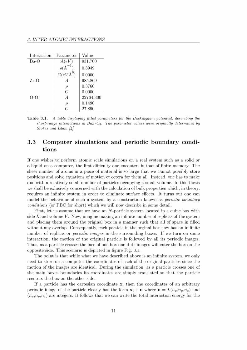
For systems that are not monatomic the strength of the interactions depends on thetype of the interacting atoms e.g. in the case of BaZrO3 the Pauli repulsion betweenBa- and O atoms will be different from the repulsion between Zr- and O atoms andso forth. Thus we end up several sets of the parameters (A, ρ,C) for the differentinteracting atomic species. For BaZrO3, an appropriate set of fitted parameters havebeen determined by Stokes and Islam [4] and are listed in the table below.
10
3. INTER-ATOMIC INTERACTIONS
Interaction Parameter Value
Ba-O A(eV ) 931.700
ρ(A−1
) 0.3949
C(eV A6) 0.0000
Zr-O A 985.869ρ 0.3760C 0.0000
O-O A 22764.300ρ 0.1490C 27.890
Table 3.1. A table displaying fitted parameters for the Buckingham potential, describing theshort-range interactions in BaZrO3. The parameter values were originally determined byStokes and Islam [4].
3.3 Computer simulations and periodic boundary condi-tions
If one wishes to perform atomic scale simulations on a real system such as a solid ora liquid on a computer, the first difficulty one encouters is that of finite memory. Thesheer number of atoms in a piece of material is so large that we cannot possibly storepositions and solve equations of motion et cetera for them all. Instead, one has to makedue with a relatively small number of particles occupying a small volume. In this thesiswe shall be exlusively concerned with the calculation of bulk properties which, in theory,requires an infinite system in order to eliminate surface effects. It turns out one canmodel the behaviour of such a system by a construction known as periodic boundaryconditions (or PBC for short) which we will now describe in some detail.
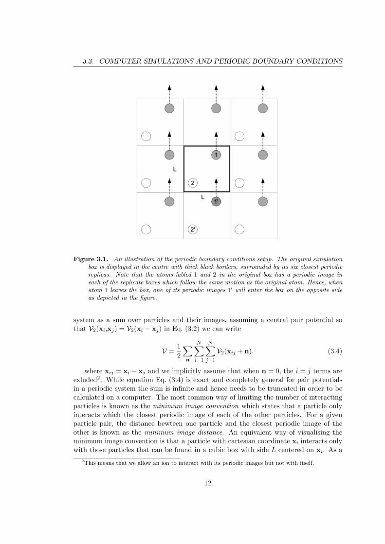
First, let us assume that we have an N -particle system located in a cubic box withside L and volume V . Now, imagine making an infinite number of replicas of the systemand placing them around the original box in a manner such that all of space in filledwithout any overlap. Consequently, each particle in the orginal box now has an inifinitenumber of replicas or periodic images in the surrounding boxes. If we turn on someinteraction, the motion of the original particle is followed by all its periodic images.Thus, as a particle crosses the face of one box one if its images will enter the box on theopposite side. This scenario is depicted in figure Fig. 3.1.
The point is that while what we have described above is an infinite system, we onlyneed to store on a computer the coordinates of each of the original particles since themotion of the images are identical. During the simulation, as a particle crosses one ofthe main boxes boundaries its coordinates are simply translated so that the particlereenters the box on the other side.
If a particle has the cartesian coordinate xi then the coordinates of an arbitraryperiodic image of the particle clearly has the form xi + n where n = L(nx,ny,nz) and(nx,ny,nz) are integers. It follows that we can write the total interaction energy for the
11
3.3. COMPUTER SIMULATIONS AND PERIODIC BOUNDARY CONDITIONS
Figure 3.1. An illustration of the periodic boundary conditions setup. The original simulationbox is displayed in the centre with thick black borders, surrounded by its six closest periodicreplicas. Note that the atoms labled 1 and 2 in the original box has a periodic image ineach of the replicate boxes which follow the same motion as the original atom. Hence, whenatom 1 leaves the box, one of its periodic images 1′ will enter the box on the opposite sideas depicted in the figure.
system as a sum over particles and their images, assuming a central pair potential sothat V2(xi,xj) = V2(xi − xj) in Eq. (3.2) we can write
V =1
2
∑n
N∑i=1
N∑j=1
V2(xij + n). (3.4)
where xij = xi − xj and we implicitly assume that when n = 0, the i = j terms areexluded2. While equation Eq. (3.4) is exact and completely general for pair potentialsin a periodic system the sum is infinite and hence needs to be truncated in order to becalculated on a computer. The most common way of limiting the number of interactingparticles is known as the minimum image convention which states that a particle onlyinteracts which the closest periodic image of each of the other particles. For a givenparticle pair, the distance bewteen one particle and the closest periodic image of theother is known as the minimum image distance. An equivalent way of visualising theminimum image convention is that a particle with cartesian coordinate xi interacts onlywith those particles that can be found in a cubic box with side L centered on xi. As a
2This means that we allow an ion to interact with its periodic images but not with itself.
12

3. INTER-ATOMIC INTERACTIONS
further restriction, one typically only includes interactions with particles within a sphere(rather than a box) of radius rcut < L/2 centered on xi. The parameter rcut is knownas the cut-off radius for the potential and must be chosen large enough that the totalinteraction energy converges. In the case of the Buckingham potential Eq. (3.2) this isachievable for relatively small values of rcut since the two potential terms decay as e−r
and 1/r6 respectively.Note that the PBC are an artificial construction and as such can introduce unwanted
correlations and distorsions in a simulation, especially when calculating forces in e.g. amolecular dynamics program. Therefore, one must avoid working with systems thatare too small. In particular for a solid such as BaZrO3 working with a single unit cellis not enough, instead we work with supercell consisting of several primitive cells (i.e.containing only a single lattice point each) packed next to each other. The size of asupercell is specified according to Nc,x×Nc,y×Nc,z where Nx is the number of primitivecells in the x-direction and so on. In this thesis we will only deal with cubic supercellsand for computational reasons they will never be larger than 4×4×4. A more detailedaccount of the concepts explained in this section can be found in [1].
3.4 An algorithm for calculating the potential
We will now make use the ideas developed in the last section and describe an algorithmfor calculating the total short-range interaction energy of the system as defined by theBucking potential. To simplify things we will consider a monatomic system withN atomstotal so that the interaction can be described by a single set of Buckingham parametersA, ρ,C. As discussed in the last section a finite system with periodic boundary conditionsmust be used and to truncate the sum Eq. (3.4) a spherical cut-off rcut is introduced.The algorithm then basically consists of looping over atom pairs and add up pairwiseinteractions provided that the minimum image distance is less than rcout. How theminimum image distance is calculated depends on where the coordinate system is locatedrelative to the simulation box. Here, there are two standard choices: a) let the origincoincide with the lower left corner of the box or b) with the centre of the box. In eithercase the minimum image distance r between two atoms with coordinate xi and xj iscalculated according to
r =∣∣∣xij − Lfround
(xijL
)∣∣∣ (3.5)
where fround denotes a function that rounds each element of a vector to the nearestinteger. The algorithm for calculating the interaction energy is summarised step by stepbelow.
Calculating the Buckingham potential1. Choose a radial cut-off which satifies the minimum image convention i.e. rcut <L/2.
2. Loop over all possible atom pairs (i,j) and for each pair do the following:
13

3.5. THE MODEL POTENTIAL PART II: LONG-RANGE INTERACTIONS ANDTHE EWALD SUMMATION
2.1. Calculate the minimum image distance r:
r =∣∣∣xij − Lfround
(xijL
)∣∣∣where xij = xi − xj
2.2. if r < rcut, add to the total potential energy V the contribution from theinteraction between atom i and j given by
δV = Ae−r/ρ − C
r6(3.6)
The most expensive element of this algorithm is clearly the evaluation of the tran-scendental exponential function. In general, much of the appeal of using a rigid-ionmodel with a pair potential is that the calculations become very cheap.
3.5 The model potential part II: Long-range interactionsand the Ewald summation
Up until this point we have only accounted for the short-range interactions in our system.In a realistic ionic system one of course also has coulombic interactions between thecharged ions. The electrostatic potential has the basic form
Φ(r) =q
r. (3.7)
For a periodic system consisting of N ions with charges {qi}Ni=1 we can write thetotal electrostatic interaction energy on the form Eq. (3.4):
Vcoul =1
2
∑n
N∑i=1
N∑j=1
qiqj|xij + n|
. (3.8)
The crucial difference is that while the terms contributing to the Buckingham po-tential decay as e−r and 1/r6 respectively, the coulomb potential only decays as 1/r.Thus if we were to adopt an identical approach to computing this electrostatic energyas we did the short-range interactions (i.e. simply truncate the sum by introducting aradial cut-off) we would have to include far too many terms in Eq. (3.8). There is alsoa more subtle problem with the 1/r decay, in mathematical terms the summation inEq. (3.8) is conditionally convergent, meaning that the result depends on the order ofthe summation. Thankfully, there is way to overcome these difficulties, namely a pow-erful technique for computing long-range interactions known as the Ewald summation.Unfortunately, the derivation is quite lengthy and as such we have chosen to place it inappendix A to which the curious reader is referred. We shall instead be content with ashort summary of the results: if the system is periodic, one can replace the summationin Eq. (3.8) with two rapidly converging sums, one in real-space and one in reciprocalspace. The final expression for the total electrostatic energy of the system is
14

3. INTER-ATOMIC INTERACTIONS
Vcoul =1
2
∑n
N∑i=1
N∑j=1
qiqjerfc(α |xij + n|)|xij + n|
+2π
V
∑k 6=0
N∑i=1
N∑j=1
qiqj exp (ik · xij)exp (−k
2
4α )
k2
− α√π
∑i
q2i
(3.9)
Here n = L(nx,ny,nz) as usual and similarily the reciprocal space vectors k aregiven by k = 2π
L (nkx ,nky ,nkz) with (nkx ,nky ,nkz) an integer vector. Since the two sumsin Eq. (3.9) (the real-space sum over n and the reciprocal sum over k) both decayrapidly we can proceed to truncate using two radial cut-offs, one in real-space andone in reciprocal space. The parameter α found in Eq. (3.9) is known as the splittingparameter and controls the relative convergence speed between the two sums. For adetailed derivation and discussion of these results the reader is referred to appendix A.An implementation of the Ewald summation in Fortran 90 can be found in appendix B.
15

CHAPTER 4
THE MONTE-CARLO METHOD
The previous chapter was dedicated to calculating the short- and long-range interactionsin our system. Combining the Buckingham potential with Coulomb potential expandedusing the Ewald summation resulted in a simple model allowing us to compute the totalinteraction energy of the system or for any one particle in the system. We would nowlike to put this knowledge to use and calculate properties, these could be e.g. thermo-dynamical quantities or properties related to the structure such as a pair correlationfunctions. Using tools from statistical mechanics, these properties can be obtained asensemble averages defined by integrals involing a probability distribution function. Theresult is a non-trivial multi-dimensional integral over phase space. In order to calcu-late such integrals efficiently on a computer, we will introduce the powerful MetropolisMonte Carlo method (MMC). The following section provides a very brief review of somebasic results from equilibrium statistical mechanics that we will need, readers that wishto refresh their knowledge on the subject are encouraged to consult one of the manyexcellent texts on the subject e.g. [5].
4.1 Ensemble averages
In classical statistical mechanics the ensemble average (or statistical average) of a quan-tity O is given by an integral
〈O〉 =
∫dΓρ(Γ)O(Γ) (4.1)
where the variable Γ denotes a point in phase space and ρ is the probability distribu-tion function. Note that for a classical N particle system a point in phase space is definedby the positions and momenta for all the N particles i.e. Γ = {x1, . . . ,xN ,p1, . . . ,pN}.In this thesis we will work exclusively in the canonical ensemble where the number ofparticles N , the volume V and the temperature T are all constant and consequently
16

4. THE MONTE-CARLO METHOD
we sometimes refer to this as the NV T -ensemble. In this ensemble the equilibriumprobability distribution function is the Boltzmann or canonical distribution
ρNVT(Γ) =1
Ze−βH(Γ) (4.2)
where β = 1kBT
and
Z =
∫dΓe−βH(Γ) (4.3)
is the partition function. Hence we can write the equilibrium average for a quantityO in canonical ensemble as
〈O〉 =
∫dΓO(Γ)
e−βH(Γ)
Z. (4.4)
The classical Hamiltonian has the form H = T + V where T =∑N
i=1pi
2mionly
depends on the momenta P = {p1, . . . ,pN} and the potential V = V(X) only dependson the positions of the particles X = {x1, . . . ,xN}. Thus the integral over e−βH(Γ) inthe partition function Eq. (4.3) can be separated into one momentum integral and oneposition (configurational) integral. If O is independent of the momenta, the integralsover P in the nominator and denominator of Eq. (4.4) will cancel and one is left withan average
〈O〉 =
∫dXO(X)e−βV(X)∫dXe−βV(X)
. (4.5)
Thus, fom here on we denote the position distribution ρNVT(X) = exp (−βV(X))/Zwith Z =
∫dXe−βV(X) and write our ensemble averages
〈O〉 =
∫dXρNVT(X)O(X). (4.6)
Multi-dimensional integrals such as Eq. (4.6) cannot be evaluated using direct nu-merical integration methods e.g. Simpson’s rule due to the sheer number of operationsthat would be required .Instead we will use a famous method based on results fromstatistics, namely the Monte Carlo method which is the topic of the next section.
4.2 Monte-Carlo integration
Monte-Carlo integration is different from most other numerical integration methods inthat it draws on results from mathematical statistics and therefore has probabilisticelements. To illustrate how the method works, consider integrating a function of onevariable f over the interval [a,b]:
I =
∫ b
adxf(x). (4.7)
17
4.2. MONTE-CARLO INTEGRATION
Let ξ be a continuous random variable with a probability density function ρ definedon [a,b] such that ρ(x) 6= 0, ∀x ∈ [a,b] and
∫ ba dxρ(x) = 1. Multiplying and the dividing
by ρ we can rewrite Eq. (4.7)∫ b
adxf(x) =
∫ b
adxρ(x)
f(x)
ρ(x). (4.8)
Recall from statistics that if g is a arbitray function the expected value of g(ξ) isgiven by
〈g(ξ)〉 =
∫ b
adxρ(x)g(x). (4.9)
Now let g be defined by g(x) = f(x)/ρ(x), from Eqs. (4.8) and (4.9) it follows that
〈g(ξ)〉 =
⟨f(ξ)
ρ(ξ)
⟩=
∫ b
adxρ(x)
f(x)
ρ(x)=
∫ b
adxf(x). (4.10)
Hence, if we can find a way to approximate the expected value 〈g(ξ)〉 we have alsofound an approximation to our original integral Eq. (4.5). The obvious approach isto randomly draw a collection of samples {ξi}Nsi=1 from the distribution ρ and thenapproximate the expected value 〈g(ξ)〉 using the sample mean of g:
〈g(ξ)〉 ≈ gNs =1
Ns
Ns∑i=1
g(ξi). (4.11)
The law of large numbers, which is a fundamental result of statistics, guaranteesthat as Ns tends towards infinity the above approximation become exact i.e.
limNs→∞
gNs = 〈g(ξ)〉 (4.12)
We call Eq. (4.11) the Monte-Carlo estimate for I. In conclusion, we have thefollowing recipe for estimating the integral Eq. (4.7):
Monte Carlo integration1. Choose an appropriate probability density function ρ.2. Generate a large collection of samples {ξi}Nsi=1 randomly drawn from ρ.
3. Compute the sample mean: 1Ns
∑Nsi=1
f(ξi)ρ(ξi)
.
4. Approximate the integral using the sample mean:∫ ba dxf(x) ≈ 1
Ns
∑Nsi=1
f(ξi)ρ(ξi)
.
The simplest choice one can make is to let ξ be uniformly distributed over [a,b] sothat ρ(x) = 1/(b− a) and ∫ b
adxf(x) ≈ b− a
Ns
Ns∑i=1
f(ξi). (4.13)
18

4. THE MONTE-CARLO METHOD
For many application this choice of ρ is far from optimal however, since every pointin the domain of integration is sampled, on average, an equal number of times. Thiscan be disadvantageous when the integrand f is only appreciable in certain regions ofthe domain and for any outlying points the integrand is small enough that only a fewsamples are actually required. The solution is to choose ρ in a way that it, to someextent, captures the behaviour of f . Such a choice of a non-uniform distribution ρ isreferred to as importance sampling and will be a crucial component in our calculations.
It is completely straightforward to generalise the results derived above to multi-dimensional integrals. If f is a function of Nd variables {x1, x2, . . . ,xNd} to be integratedover D ⊂ RNd and ρ = ρ(x1, x2, . . . ,xNd) a suitable (joint) probability density we canproceed in the exact same manner as above. The resulting estimate of the integral is∫
Ddx1 . . . dxNdf(x1, x2, . . . ,xNd) ≈
1
Ns
Ns∑i=1
f(ξi)
ρ(ξi)(4.14)
where {ξi}Nsi=1 are drawn from the multi-dimensional probability density ρ. It is when
the number of variables becomes large and the integrand is appreciable only over certainregions of the domain D that Monte-Carlo integration really shines. Taking a look atthe ensemble average
〈O〉 =
∫dXρNVT(X)O(X) (4.15)
from the previous section Section 4.1 we can see that it fits the profile for an idealMonte-Carlo case perfectly: with N particles there are 3N coordinates that we need tointegrate over. Furthermore, if the energy happens to be large for a particular configura-tion the integrand will be vanishingly small due to the inverse exponential in ρNVT. Wecan now write the Monte-Carlo estimate for Eq. (4.15). The integrand is ρNVT(X)O(X)and if ρ is an arbitrary probability density, we have according to Eq. (4.10)
〈O〉 =
⟨ρNVTOρ
⟩(4.16)
A suitable choice for ρ is to simply let ρ = ρNVT. Since the canonical distributionvaries exponentially with the energy it ought to give a good indication of where theintegrand ρNVTO is significant for most forms of O. From Eq. (4.11) the Monte-Carloestimate then reduces to
〈O〉 ≈ 1
Ns
Ns∑i=1
O(ξi) (4.17)
where {ξi}Nsi=1 are now randomly drawn from the canonical distribution ρNVT. Let
us take a step back and look at what we have accomplished. When we set out at thebeginning of Section 4 the goal was to be able to calculate properties of the BaZrO3
system, such as thermodynamical quantities or correlation functions. These propertieswere then expressed as ensemble averages in Section 4.1, which subsequently forced us
19
4.2. MONTE-CARLO INTEGRATION
to consider efficient ways to computing multi-dimensional integrals, finally leading us tothis section and Monte-Carlo integration. The techniques developed here have led usto Eq. (4.17) and hence the only problem left is how to generate samples ξi from thecanoncial distribution.
Before moving on to solving the problem of how to sample the canonical distribution,we will briefly discuss the error associated with a Monte Carlo estimate since the methoddoes us no good unless it can produce approximations to the integral I with small errors.Going back to our one-dimensional example, the variance of g(ξ) = f(ξ)/ρ(ξ) is definedas
Var [g(ξ)] =⟨g(ξ)2
⟩− 〈g(ξ)〉2 (4.18)
and the standard deviation is σ(g(ξ)) =√
Var [g(ξ)]. It follows from the central limit
theorem that if the samples {ξi}Nsi=1 are statistically independent then the sample meangNs in Eq. (4.11) is approximately gaussian distributed with variance
Var [gNs ] =Var [g(ξ)]
Ns. (4.19)
The error incurred by replacing the exact integral I with the Monte Carlo estimateEq. (4.11) is then given by the standard deviation
σ [gNs ] =σ [g(ξ)]√
Ns. (4.20)
Eq. (4.20) tells us that the error decreases as the square root of the number of sampleswherein lies the power of Monte Carlo integration. We note further that in the case of noimportance sampling i.e. ρ ≡ 1 then g(ξ) = f(ξ) and the error is σ [f(ξ)] /
√Ns, but if we
choose ρ so that it captures the behaviour f then σ [g(ξ)] < σ [f(ξ)] and we decrease theerror. Eq. (4.19) relies on the assumption that the samples are statistically independentwhich is not true in a MMC simulation where new configurations are generated fromold ones inducing a high amount of correlation. To account for this we introduce thestatistical inefficieny s which can be interpreted as the number of MC steps betweentruly independent configurations i.e. Ns/s is the number of statistically independentsamples. We can estimate s using block averaging. Let Nb be the block size and definethe j:th block average of g:
Gj =1
Nb
Nb∑i=1
gi+(j−1)Nb (4.21)
where gi ≡ g(ξi). An estimation of s is then given by
s = limNb→large
NbVar[G]
Var[g](4.22)
We then replace Eq. (4.19) with
20

4. THE MONTE-CARLO METHOD
Var [gNs ] = sVar [g(ξ)]
Ns. (4.23)
and the MC error estimate is given by the corresponding standard deviation.
4.3 The Metropolis-Hastings algorithm
In the previous section we used Monte Carlo integration and importance sampling toshow that ensemble averages can be computed in an efficient way provided that wecan find a method for sampling the canonical distribution. To accomplish this we willnow introduce the Metropolis-Hastings algorithm, which is essentially a biased randomwalk through phase space that after an initial equilibration period will start to generatesamples distributed according to ρNVT. Starting from an initial state Γ0, new states arechosen with a probability given by a transition rule
P(Γm → Γn) (4.24)
i.e. Eq. (4.24) is interpreted as the probability of transitioning from the state Γmto Γn. Note that the transition probability only depends on current state and notany of the previous states, in other words the random walk is memoryless and we saythat it constitutes a Markov chain. For a finite state space {Γ0,Γ1, . . .} an arbitrarydistribution can then be defined by a vector ρ where the m:th element ρm gives theprobability of finding the system in state Γm. Similarily, we can regard the transistionrule Eq. (4.24) as a matrix P with elements Pnm ≡ P(Γm → Γn) (note the intentionalreversal of the order of the labels m and n in this definition). Each individual column ofP sum up to unity and we call a matrix with this property a stochastic matrix. If thedistribution at step k of the walk is ρ(k), making a transition according to P will thusalter the distribution and the new distribution is given by a matrix multiplication
ρ(k+1) = Pρ(k). (4.25)
In this notation the limiting distribution ρ(∞) is
ρ(∞) = limk→∞
Pkρ(0) (4.26)
where ρ(0) denotes the initial distribution. From Eq. (4.26) it is apparent that ρ(∞)
is a solution to the eigenvalue equation
Pρ(∞) = ρ(∞) (4.27)
One can prove [1] that if the transition rule is defined in a way such that the resultingMarkov chain is ergodic, meaning that any one state of the system can be reached in afinite number of transitions regardless of the intial state, then Eq. (4.27) has a uniquesolution. In the Metropolis-Hastings algorithm, one chooses the transition rule P so
21
4.3. THE METROPOLIS-HASTINGS ALGORITHM
that the limiting distribution is given by canonical distribution ρ(∞) = ρNVT. Moreprecisely, P is constructed to statisfy the condition of detailed balance
ρmPnm = ρnPmn. (4.28)
Summing over n in Eq. (4.28) we find that the left-hand side∑
n ρmPnm = ρm sincethe sum over a column of P is unity as noted above and hence∑
n
Pmnρn = ρm. (4.29)
But this is just Eq. (4.27) again and we can conclude that if P satisfies detailedbalance (and has columns which all sum to unity) the Markov chain will converge to aunique distribution. The next step is to write P(Γm → Γn) as the product of a trialtransition T (Γm → Γn) and an acceptance probability A(Γm → Γn):
P(Γm → Γn) = T (Γm → Γn)A(Γm → Γn) (4.30)
or in matrix form
Pnm = TnmAnm. (4.31)
In the traditional Metropolis-Hastings algorithm the trial transition has the form ofa randomly proposed movement for a single atom and whether the proposed movementis accepted or not is subsequently determined by the acceptance probability. Thus,consider an atom labled i with a coordinate xmi and a box B centered around xmi withside δl. A new position xni for this atom is then proposed with probability
Tnm =
{1/Ncube, xni ∈ B
0, otherwise(4.32)
where Ncube is the total number of states insibe B which is, of course, finite ona computer. Eq. (4.32) means that we propose a new position for an atom with uni-form probability inside a box with side δl centered around the atoms current location.Whether to accept this movement or not is then determined by the acceptance proba-bility A defined for m 6= n as
Anm =
1,ρNVT(X←xni )ρNVT(X←xmi ) ≥ 1
ρNVT(X←xni )ρNVT(X←xmi ) , otherwise
(4.33)
where X = {x1, . . . ,xN} are the current positions of all the atoms as usual. Thenotation X← xni indicates that we replace the coordinate of atom i with xni in the con-figuration X, but keep the configuration otherwise unchanged. When defined in this waythe acceptance probability is symmetric and it follows that the complete transition rulewill satisfy detailed balance [1]. From section Section 4.1 ρNVT(X) = exp [−βV(X)] /Zso it follows that
22

4. THE MONTE-CARLO METHOD
ρNVT(X′)
ρNVT(X)=
exp [−βV(X′)] /Z
exp [−βV(X)] /Z= exp
[−β(V(X′)− V(X)
)]. (4.34)
If we define the difference in potential energy ∆V = V(X ← xni ) − V(X ← xmi ) wecan rewrite the acceptance probability Eq. (4.33) using Eq. (4.34):
Anm =
{1, ∆V ≤ 0
exp [−β∆V] , otherwise(4.35)
We have now arrived at the final form of the acceptance probability, combining thiswith the trial transition Eq. (4.32) yields a complete transition rule which can be usedto generate a random walk in phase space that will eventually converge in the sensethat the generated states are sampled from the canonical distribution. One of the mainreasons that the Metropolis-Hastings algorithm is so effective is that there is no needto compute the normalisation factor 1/Z for the canonical distribtuion since this factoris cancelled in Eq. (4.34) and we only have to worry about computing the difference inpotential energy. Furthermore, since only a single atom is moved in each step, if we havea pair potential ∆V can be obtained by subtracting the potential energy of the atombeing moved in old configuration from the potential energy of the same atom in the newconfiguration:
∆V = V(X← xni )− V(X← xmi ) =
N∑j 6=i
[V2(xni − xj)− V2(xmi − xj)
](4.36)
Here we have used again the notation introduced in Section 3.1 Eq. (3.2) whereV2(xi−xj) represents the pairwise interaction (short-range as well as coulombic) betweenatoms i and j. Eq. (4.36) means that at no point in our algorithm are we forced tocompute the total interaction energy for the entire system.
4.4 The complete Metropolis Monte Carlo algorithm
We will now combine the results from Sections 4.1, 4.2 and 4.3 into a single powerfulalgorithm. The algorithm is quite general but to make things more concrete we willcomment on what some of the steps entail for our BaZrO3 system. When combining theMetropolis algorithm with Monte Carlo integration one speaks of a Metropolis MonteCarlo (MMC) or a Markov-Chain Monte Carlo (MCMC) method. For applications inphysics when the limiting distribution is the Boltzmann distribution the name canonicalMonte Carlo is also used sometimes, in this thesis we shall stick with the name MetropolisMonte Carlo however. The full algorithm is summarised below, note that we havedispensed with the superscript indices used in the previous section and now write theold position of an atom i as xold
i and similarily the new position after a trial displacementis denoted xnew
i .
23

4.4. THE COMPLETE METROPOLIS MONTE CARLO ALGORITHM
The Metropolis Monte Carlo method1. Initialise the postions of all the N atoms. For a liquid or a solid such as BaZrO3
an appropriate choice would be to use the T = 0 equilibrium configuration.2. Choose at random an atom i with coordinate xold
i and generate a trial state bydisplacing it symmetrically according to xnew
i = xoldi + δl(2η − 1) where η is ran-
dom vector drawn from the uniform distribution on [0,1]. Note that simultaneousstorage of the both new and old coordinate is required at this point.
3. Compute the difference in potential energy: ∆V = V(X ← xnewi )− V(X ← xold
i ).If the potential consists of pairwise interactions use Eq. (4.36).
4. If ∆V ≤ 0 the trial state is immediately accepted and the old coordinate can bedeleted. If ∆V > 0 generate a uniform random number q in [0,1]:
4.1. If q ≤ exp (−β∆V) the trial state is accepted and the old position can bedeleted.
4.2. Else if q > exp (−β∆V) the trial state is rejected and the atom’s old positionmust be restored.
5. After one or several atoms have been moved, update the average value of anyproperty of interest O(X), note that all moves contribute equally to the averagei.e. regardless of whether the old position was restored or the trial state wasaccepted. Also update the error.
6. Repeat steps 2 to 5 a large number of times.7. Compute the ensemble average of O by normalising with the number of times the
code has passed through step 5. Also compute the errorbars.
A few comments are appropriate here. Firstly, in step 1 we could instead give eachatom a random starting position in the simulation box but this would slow down theconvergence since we would begin from an extremely unlikely starting configuration. Fora solid going to a non-zero temperature below the melting point means that the atomswill vibrate around their equilibrium position and hence intialising the system using thisconfiguration is a better approach. In steps 2 through 4 we make a transition accordingto the rule defined by Eqs. (4.32) and (4.35), and it is important to note that if the trialstate is rejected we keep the old configuration which still contributes to the average instep 5.
If we are doing a simulation at non-zero T the starting configuration, no matterhow well we chose it, will still be in an unlikely state and hence there is a certainthermalisation period before we start to sample the correct distribution. To adjust forthis we can start by running the simulation without actually updating the averages.We call this the equilibration period and it usually extends over a number of stepscorresponding to a few multiples of the thermalisation period. After equlibration whenwe are sure that the correct distribution is being sampled we start to record O(X).Sometimes when updating O(X) is an expensive operation in itself one typically waitsuntil several moves have been accepted before updating the average, see step 5 above.It is convenient to divide an MC simulation into cycles, where one cycle constitutes Nattempted one atom moves meaning that a trial movement has been proposed for each
24

4. THE MONTE-CARLO METHOD
atom in the system on average once. Properties O which are expensive to calculate areusually only updated once each MC cycle.
There is also the question of the free parameter δl, which controls the maximumlength of the trial displacement in any direction. If we choose a very small δl we willfind that more moves tend to be accepted since the change in potential energy will notbe as big. This might lead to slow convergence since the atoms are only allowed to takevery small steps toward the optimal configuration. We might also worry that we are notsampling the correct distribution since unlikely moves will be accepted more frequentlyas well. Conversely, if we choose δl very large, we will find that only a small number ofmoves are accepted and in this case we might not be exploring a large enough region ofphase space in order to get a reliable estimate of the ensemble average. To be on thesafe side it is therefore common practice to tune the δl parameter so that roughy half ofthe trial moves are accepted.
4.5 The pair correlation function
As an important example of a property that can be calculated using the canonicalMonte Carlo Method we will consider the pair correlation function g, which describesthe distribution of atomic pairs in the system. More precisely, in the canonical ensemblewe define the pair correlation as the integral
g(x1,x2) =V 2(N − 1)
NZ
∫dx3dx3 . . . dxNe
−βV(X) (4.37)
This equation can be cast in an equivalent form that shows clearly how to calculate gin a MC simulation. Integrating over the remaining two coordinates to get an ensembleaverage and introducing δ-functions to compensate we see that, since the choice of x1
and x2 is arbitrary provided the system in monatomic, Eq. (4.37) can be rewritten
g(r) =1
ρ2
⟨∑i
∑j 6=i
δ(xi)δ(xj − x)
⟩=
V
N2
⟨∑i
∑j 6=i
δ(x− xij)
⟩(4.38)
with r = |x|. From Eq. (4.38) it is clear that g(r) can easily be calculated using thecanonical MMC method, all we have to do is to discretise the δ-function and then averagethe sum V
N2
∑Ni=1
∑Nj=1 δ(r−|xi − xj |) over a large number of configurations. To do this
we loop over all atomic pairs and calculate the corresponding distances while collectingall the occurences in a histogram. A Fortran 90 program for calculating g(r) has beenimplemented and can be found in appendix B. Section 6 contains some examples of g(r)for our BaZrO3 system.
25

CHAPTER 5
QUANTUM STATISTICAL MECHANICS AND PATHINTEGRALS
Thus far we have studied atomic systems from a classical viewpoint using the languagestatistical mechanics. As mentioned in the introduction, a classical treatment of thenuclear motion is not always a valid assumption. In general, quantum effects are mostlyimportant when the temperautre is low and the system consists of lighter atoms such ashydrogen or helium. However, when there are competing structures with small energydifferences such as in e.g. barium zirconate which has AFD phases it is not obvious thatquantum effects can be neglected. In this section we will show how to treat the nuclearmotion using quantum statistical mechanics, the first point of order to develop thedensity operator formalism. The density operator contains in principle all informationwe need about the system (it is analogous to the propagator) and by expanding this intoa so called path integral we will be able to compute it numerically.
5.1 The density operator
In Section 4.1 we saw that in classical statistical mechanics the fundamental quantitityis the probability distribution which can be integrated to yield the probability of findingthe system in a certain region of phase space. With knowledge of the probability densityone can proceed to define e.g. thermodynamical quantities or transport properties asaverages over phase space. In quantum statistical mechanics the density operator playsa similar role and generalises the concept of a wave function. More precisely, the densityoperator describes statistical mixtures of states. As an easy example consider a spin-1
2system and suppose that we know that with probability P1 the state is | ↑〉 and withprobability P2 = 1 − P1 the state is | ↓〉. We call this a statistical mixture of | ↑〉 and| ↓〉 states or simply a mixed state, while e.g. | ↑〉 is referred to as a pure state. Notethat a statistical mixture is fundamentally different from a superposition of | ↑〉 and| ↓〉 inasmuch as any such linear combination will have a definite spin direction. To
26
5. QUANTUM STATISTICAL MECHANICS AND PATH INTEGRALS
be able to describe statistical mixtures of states we will introduce the density operatorformalism.
A statistical mixture of states is specified by a set of state kets {|ψi〉} with corre-sponding probabilities Pi. The density matrix is defined as
ρ =∑i
Pi|ψi〉〈ψi|. (5.1)
If the weights Pi in the above equation are to be interpreted as probabilities they mustsatisfy the normalisation condition
∑i Pi = 1 which gives a corresponding normalisation
condition for the density operator itself
tr(ρ) = 1. (5.2)
We are often interested in determining the average of an observable O since these are thevalues one can measure. For a pure state this average would simply be the expectationvalue of O but for a mixed state the natural definition is to weigh the expectation valuesof O taken relative to states |φi〉 with the corresponding probabilities Pi and then sumover all such terms:
〈O〉 =∑i
Pi〈ψi|O|ψi〉. (5.3)
Eq. (5.3) is the quantum mechanical equivalent to the classical ensemble averageEq. (4.1). To illustrate the usefulness of the density operator we will now show that itcan be used to calculate the ensemble average Eq. (5.3). To see how this is done we willrewrite Eq. (5.3) in an arbitrary basis {|b〉} using the completeness relation
∑b |b〉〈b| = 1:
〈O〉 =∑b
∑b′
(∑i
Pi〈b|ψi〉〈ψi|b′〉
)〈b′|O|b〉
=∑b
∑b′
〈b|ρ|b′〉〈b′|O|b〉 = tr(ρO)
(5.4)
where we recognise the expression enclosed by paratheses in the first line as the matrixelement of the density operator written in the basis {|b〉}. Often the use of a basis isimplied and one then simply refers to ρ as the density matrix. Equation Eq. (5.4) statesthat in order to calculate the ensemble average of O we simply need to take the traceof the matrix product of ρ and O and since the trace is independent of the basis we canwork in whatever basis happens to be convenient.
5.2 The thermal density matrix
Consider a system in thermal equilibrium at temperature T where the number of parti-cles N and volume V are constant. In what follows all the particles in our system are
27
5.2. THE THERMAL DENSITY MATRIX
assumed to be distinguishable so we can disregard bose and fermi statistics. Further-more, suppose the exact energy eigenstates and eigenvalues are |φn〉 and En i.e.
H|n〉 = En|n〉. (5.5)
From statistical mechanics we know that the appropriate probability distribution forthis type of system is the canonical distribution which gives the probability of findingthe system in a state with energy En as
Pn =e−βEn
Z(5.6)
where the normalising constant Z =∑
n e−βEn is the partition function and β = 1
kBTas usual. The density operator can then be written
ρ =∑n
e−βEn
Z|n〉〈n| = e−βH
Z. (5.7)
In literature on quantum statistical mechanis is somewhat of a convention to omit thepartition function Z in the above equation and refer to
ρ = e−βH (5.8)
as the thermal density operator. This convention will be followed for the rest of this re-port. As an imidiate consequence of Eq. (5.8), note that the partition function is relatedto the thermal density matrix 1 through Z = tr(ρ) and the average 〈O〉 = 1
Z tr(ρO).With these results one can proceed to identify familiar thermodynamic quantitites withoperator averages. To illustrate this consider the internal energy E of the system whichis identified with 〈H〉:
E = 〈H〉 =1
Ztr(ρH) =
∑n
(Ene
−βEn
e−βEn
)=∑n
(− ∂
∂βln(e−βEn
))= − ∂
∂βln(Z).
(5.9)
This should be a familiar formula to any student of thermodynamics. When performingcalculations, especially on a computer, one often works in the position-space representa-tion. The thermal density matrix matrix element at temperature T is then a continuousfunction
ρ(X,X′;β) = 〈X|ρ|X′〉 (5.10)
1Since unnormalised weights are being used for the density matrix the trace is no longer unity.
28

5. QUANTUM STATISTICAL MECHANICS AND PATH INTEGRALS
where X = {x1,x2, . . . ,xN} are the coordinates of all the N particles in the system. Itis sometimes useful to express the thermal density matrix using the eigenenergy wave-functions φn(x) = 〈x|n〉, Eq. (5.10) then reads
ρ(X,X′;β) =∑n
φ(X)∗φ(X′)e−βEn . (5.11)
Using the completeness relation for the position base kets∫dX|X〉〈X| = 1 (5.12)
the average of an observable O in position-space becomes
〈O〉 = tr(ρO) =1
Z
∫dXdX′ρ(X,X′;β)〈X′|O|X〉. (5.13)
Similarily, the parition function is written
Z = tr(ρ) =
∫dX〈X|ρ|X〉. (5.14)
Before moving on to the much anticipated path integrals we will consider a simple, yetimportant, example of a thermal density matrix, namely that of a free particle in acubic box with side L and periodic boundary conditions. From elementary quantummechanics we know that the solutions to the Hamiltonian eigenvalue problem are planewaves φk(x) = 1√
Veik·r where the wave vectors are given by k = 2π
L n with n an integer
vector. The associated eigenenergy values are Ek = ~2k2
2m . Together with Eq. (5.11)these results allow us to write the free particle density matrix
ρ(x,x′;β) =1
V
∑k
e−βλk2e−ik·(x−x′) (5.15)
where λ = ~22m if we write the ~ explicitly2. This expression can be simplified somewhat
if we assume that the thermal de Broglie wavelength Λ ≡√βλ� L. Λ is approximately
the de Broglie wavelength of the particle at temperature T and we are thus assumingthat this wavelength is much smaller than the size of the box. This means that thek-values are densely packed in the k-space volume (2π)3/V and the sum in Eq. (5.15)can be replaced by an integral 1
V
∑k −→
∫dk
(2π)3. Note that this approximation only
becomes exact in the limit of an inifinite box and thus fails to account for the periodicboundary conditions. Carrying out the integration the result is
ρ(x,x′;β) =1
(4πλβ)3/2exp
((x− x′)2
4λβ
). (5.16)
The generalisation to N free particles is trivial:
2Here we briefly deviate from the use of atomic units so the reader can get some sense of where the~ factor will appear in the final equation
29

5.3. PATH INTEGRALS
ρ(X,X′;β) =1
(4πλβ)3N/2exp
((X−X′)2
4λβ
)=
1
(4πλβ)3N/2exp
(N∑i=1
(xi − x′i)2
4λβ
) (5.17)
5.3 Path integrals
Before doing anything, let us assess our current situation. In order to incorporatequantum effects into our simulations we have been forced to abandon the region ofclassical statistical mechanics and venture into the quantum regime. The thermal densitymatrix in principle contains all the information necessary in order to calculate any desiredproperty of the system. We were also able to calculate the thermal density matrix in thesimple case of a system of N free particles confined to a cubic box but it is clear (sincesolving for the density matrix of anN -particle system is at least as complicated as solvingthe N -particle Schrodinger equation) that we, in general, cannot hope to find analyticalsolutions. As so often happens, one is thus forced to resort to numerical methods. Thereare plenty available but we shall focus on a particularily powerful method known as thePath Integral Monte-Carlo method, or PIMC for short. The starting point of the PIMCmethod is the expansion of the density matrix in a path integral. The result will be aseemingly much more complicated expression than what we have encountered so thus far.By serendipity however, it turns out that the path integral expression is very amendableto numerical calculations. The brief presentation of the subject found here is based ona more detailed account by Ceperley [2] to which the curious reader is referred. Beforegetting into the details let us record one essential property of the density matrix:
e−(β1+β2)H = e−β1He−β2H (5.18)
i.e. the taking the product of two density matrices we obtain a new density matrixat a lower temperature. To write Eq. (5.18) in the position-space representation, applythe completeness relation Eq. (5.12) between the two density matrices in the right-handside of Eq. (5.18):
ρ(X1,X3;β1 + β2) = 〈X|ρ(β1)ρ(β1)|X′′〉
=
∫dX2ρ(X1,X2;β1)ρ(X2,X3;β2)
(5.19)
Now, imagine we would like an expression for the density matrix at temperature T , bymaking repeated use of the property Eq. (5.18) this density matrix can be written as aproduct of M density matrices at a higher temperature M × T i.e.
e−βH =(e−τH
)M(5.20)
30

5. QUANTUM STATISTICAL MECHANICS AND PATH INTEGRALS
where τ = βM . To write this in position-space one simply repeats the process used to
reach Eq. (5.19): connect all the density operators on the right-hand side of Eq. (5.20)by integrals using the completeness relation and then squeeze the result in between a braand a ket to obtain a matrix element. The resulting expression for the thermal densitymatrix at temperature T is
ρ(X0,XM ;β) =
∫dX1dX2 · · · dXM−1ρ(X1,X2; τ)ρ(X2,X3; τ) · · · ρ(XM−1,XM ; τ)
(5.21)This is our basic path integral. It is customary to refer to τ = β
M as the time step and toXk = {x1k,x2k, . . . ,xNk} as the k:th time slice. Two neighbouring slices are separated bya time step τ and hence we can assign a time tk = kτ to slice Xk. From this viewpoint,Eq. (5.21) is a ”sum” over discrete paths where a path is essentially a trajectory of thesystem: {X0,X1, . . . ,XM}. Note that referring to τ as the time step can be somewhatmisleading since we are not actually talking about the real time in the quantum systemand has the units of inverse energy. The terminology derives from the pure state QMpath integrals where one derives an expression identical to Eq. (5.21) for the propagatorof the system, in which case one would really be dealing with a time step.
The expression Eq. (5.21) looks very complicated but, as it turns out, it is possible tofind a reasonably accurate and cheap-to-compute approximation to the density matrixif the temperature is high. This means that if we choose M so that MT is large enoughwe can replace all the density matrices on the right-hand side of Eq. (5.21) using thisapproximate expression and (hopefully) still obtain a reasonable approximation to thelow temperature density matrix on the left-hand side. Thus, while all results havebeen exact up to this point we will now introduce some approximations. The Hamiltonoperator is the sum of the kinetic energy operator and a potential energy operatorH = T +V. From the Baker-Campbell-Hausdorff lemma it follows that for two operatorA and B:
eAeB = eA+B+ 12
[A,B]+H.O.T. (5.22)
Letting A = −τT and B = −τV in Eq. (5.22) yields
e−τT e−τV = e−τ(T +V)+ τ2
2[T ,V]+H.O.T. (5.23)
Thus, neglecting all commutators between T and V we have the following approximation
e−τ(T +V) ≈ e−τT e−τV (5.24)
Since this approximation means throwing away a term that is second order in τ wecan improve the accuracy by increasing M .In path integral litterature Eq. (5.24) isreferred to as the primitive approximation. We can now approximate the density matrixat temperature MT :
ρ(X,X′′; τ) ≈ 〈X|e−τT e−τV |X′′〉 =
∫dX′〈X|e−τT |X′〉〈X′|e−τV |X′′〉 (5.25)
31
5.3. PATH INTEGRALS
As usual, we are working in the canonical ensemble with a system of distinguishableparticles confined to a cubic box with periodic boundary conditions, it follows that thefirst matrix element on the right-hand side of Eq. (5.25) is the free particle densitymatrix given by Eq. (5.17):
〈X|e−τT |X′〉 ≈ 1
(4πλτ)3N/2exp
((X−X′)2
4λτ
). (5.26)
The ”≈” sign serves to remind us that Eq. (5.26) holds if the thermal de Broglie wave-length Λτ ≡
√τλ � L. Now assume that V and H commute (this is usually the case),
and can thus be simultaneously diagonalised, so that V|X〉 = V(X)|X〉. For the secondmatrix element on the right-hand side of Eq. (5.26) this means
〈X′|e−τV |X′′〉 = e−τV(X′′)δ(X′ −X′′). (5.27)
Upon substituting Eqs. (5.27) and 5.26 into Eq. (5.25) one finds that
ρ(X,X′′; τ) ≈ 1
(4πλτ)3N/2e
(X−X′′)24λτ e−τV(X′′). (5.28)
This is the desired approximation to the high temperature density matrix, valid in theprimitive approximation Eq. (5.24). Returning to Eq. (5.21) we can now write thispath integral in the primitive approximation using Eq. (5.28) to replace all the matrixelements on the right-hand side of Eq. (5.21), the result is
ρ(X0,XM ;β) ≈ 1
(4πλτ)3NM/2
∫dX1dX2 · · · dXM−1 . . .
exp
(−τ
(M∑k=1
(Xk −Xk−1)2
4λτ2+ V(Xk)
)) (5.29)
Since we have now made use of the approximation Eq. (5.28) a total of M timesthere seems to be a possibility of accumulating an error when M becomes large. This isnot the case however and in fact taking the limit M → ∞ the error goes to zero. Thisis expressed in the Trotter formula [15]
e−β(T +V) = limM→∞
(e−
βMT e−
βMV)M
. (5.30)
To simplify our notation we will refer to the two neighbouring time slices (Xk−1,Xk)as the k:th link and then define the action of this link as
Sk−1,k =
((Xk −Xk−1)2
4λτ+ τV(Xk)
). (5.31)
The total action is then obtained by summing over all the links: S =∑M
k=1 Sk−1,k.Note that the specific form of the action given in Eq. (5.31) is dependent on the ap-proximation made in Eq. (5.24). The general definition of the action is Sk−1,k =
32

5. QUANTUM STATISTICAL MECHANICS AND PATH INTEGRALS
−ln (ρ(Xk−1,Xk)) and one then refers to the expression Eq. (5.31) as the primitiveaction.
With Eq. (5.31), we can write Eq. (5.29) in the shorthand notation
ρ(X0,XM ;β) ≈ 1
(4πλτ)3NM/2
∫dX1dX2 · · · dXM−1 exp
(−
M∑k=1
.Sk−1,k
)(5.32)
In particular, the partition function becomes
Z ≈ 1
(4πλτ)3NM/2
∫dX1dX2 · · · dXM−1dXM exp
(−
M∑k=1
Sk−1,k
)∣∣∣∣X0=XM
(5.33)
The point here is that looking at the integrands in Eqs. (5.32) and (5.33), we see thatthey remain positive at all temperatures and are very reminiscent of a configurationalintergral for a classical system, see Section 4.1. This suggests the use of Monte-Carlosimulations in order to compute the integrals.
5.4 The classical isomorphism
By careful interpretation of Eqs. (5.32) and (5.33) it turns out that we can map ourquantum system to a classical polymer system. Burrowing some terminology from themathematical theory of abstract spaces this map is referred to as an isomorphism. Tosee how such a connection can arise, we need to take a closer look at the differentinteractions in the quantum system. The kinetic part of the interaction found in theexponential in Eq. (5.29) is
M∑k=1
(Xk −Xk−1)2
4λτ2=
M∑k=1
N∑i=1
(xik − xik−1)2
4λτ2=
N∑i=1
(M∑k=1
(xik − xik−1)2
4λτ2
). (5.34)
Looking closely at the expression enclosed by parantheses in Eq. (5.34) we can seethat it has the same form as the potential for a set of particles {xik}Mk=1 where eachparticle xik is coupled to its closest neighbours xik−1 and xik+1 by springs. Hence wecan think of each atom i as a sort of polymer consisting of M particles which we referto as beads. We should keep in mind that a set of beads {xik}Mk=1 really represents thecoordinates of a single atom i in the different time slices. As we saw an example ofin Section 5.2, many thermodynamical quantities are directly related to the partitionfunction. In this case we need to take the trace of the density matrix and only diagonalelements are involved. The same is true for quantities that are diagonal in position-spacelike the pair correlation function. We must thus take the trace in Eq. (5.29) i.e. integrateover XM and let X0 = XM in the integrand. Correspondingly in the polymer system,the first and last bead belonging to a particular chain must be identical, resulting in
33

5.4. THE CLASSICAL ISOMORPHISM
a ring polymer. The words polymer and chain will be used interchangeably and a ringpolymer is thus sometimes referred to as a closed chain. Later on we will also encouteropen polymers which will also be called open chains.
There is also a potential interaction in the polymer system, from Eq. (5.29) we seethat this interaction has the form
M∑k=1
V(Xk) =1
2
M∑k=1
N∑i=1
N∑j=1
V2(xik − xjk)
. (5.35)
In the ring polymer system we interpret this as a potential interaction betweenequally labeled beads belongning to different atoms. Hence the potential interaction inthe quantum system translates to a rather peculiar potential interaction in the poly-mer system, where only beads in same time slice as allowed to interact. The differentinteractions in the polymer system are represented pictorially in Fig. 5.1.
Figure 5.1. An illustration of the classical isomorphism in one dimension. The figure depictstwo atoms, each represented as a polymer consisting of five beads. The kinetic interactionbetween neighbouring beads belonging to the same atom is represented by springs. Thepotential interaction between beads which are in the same time slice (as indicated by thenumbers) but belong to different atoms is represented by double arrows. Also note thataccording to Eq. (5.33) the first and last bead are connected so that each atom is representedby a ring polymer.
With the classical isomorphism we realise that in order to compute the path integral
34
5. QUANTUM STATISTICAL MECHANICS AND PATH INTEGRALS
we can just do a classical Metropolis Monte Carlo simulation for a ring polymer systemwith interactions described by Eqs. (5.34) and (5.35). A more thorough explanationof the algorithm will be given in following section. As a final remark, the assumptionof distinguishable particles that we have made makes the situation considerably easier.Including bose statistics would further complicate the picture of the paths given abovewhile taking fermi statistics into account comes with an infamous sign problem, see [2].
5.5 The path integral Monte Carlo method
We will now describe in detail how to perform Monte-Carlo simulations to computeconfigurational integrals in the path integral formalism. As we saw in Section 5.4 thequanutm system can be mapped to classical ring polymer system with interactions de-fined by Eqs. (5.34) and (5.35). It therefore suffices to do a classical canonical Monte-Carlo simulation of this polymer system, which means that only a few modifications tothe algorithm presented in Section 4.4 are necessary. Firstly, since each atom is nowrepresented by M beads, there are NM beads total and 3NM coordinates that we needto store. Note that since we have a ring polymer system the first and last slice areidentical i.e. X0 = XM and hence we only store one of them which explains why we useM beads rather than M + 1. For the trial moves, the simplest approach is to propose adisplacement for one bead at a time in exactly the same way as we did for the atoms inthe classical simulation. The major difference instead comes during the rejection stepsince there is now a new harmonic interaction given by Eq. (5.34) that we must calculateand take into account. Consider then moving a single bead located at xold
ik to a newposition xnew
ik . In PIMC simulation it is customary to refer to the action or difference inaction rather than the interaction energy, the distinction being that one multiplies theinteraction energy by τ to obtain the corresponding action 3. To compute the change inpotential action we need only look at slice k since the potential action is local to eachslice according to Eq. (5.35), thus we get
∆Spot = τ(V(Xk ← xnew
ik )− V(Xk ← xoldik )). (5.36)
Note that much like in Section 4.4, if we have a pair potential there is no need tocompute the potential action for the entire configuration in the current slice since notall beads are moving. We can thus save a lot of effort by computing the potential actiondifference as
∆Spot = τ
N∑j 6=i
[V2(xnew
ik − xjk)− V2(xoldik − xjk)
]. (5.37)
For the kinetic part of the action we need only look at the current atom i to whichthe bead with label ik belongs, since according to Eq. (5.34) only beads belonging to the
3Note that the action quantity as defined here is dimensionless since τ has the unit of inverse energy(rather than having units of energy × time).
35

5.5. THE PATH INTEGRAL MONTE CARLO METHOD
same atom are connected by springs. The bead ik is then a part of two links, namely(xik−1,xik) and (xik,xik+1) and the change in potential action is therefore
∆Skin =1
4λτ
[(xnewik − xik−1)2 + (xnew
ik − xik+1)2 (5.38)
−(xoldik − xik−1
)2−(xoldik − xik+1
)2].
Whenever k = 1 in Eq. (5.49) we simply set k − 1 = M in agreement with the ringpolymer condition and conversely if k = M we set k + 1 = 1. Now, the total changein action is ∆S = ∆Spot + ∆Skin and hence the correct Boltzmann factor to use whentesting whether to accept or reject the proposed move is exp (−∆S). For clairty’s sakeall the steps in the Path integral Monte-Carlo method are summarised below.
The Path integral Monte Carlo method1. Initialise the postions of all the NM beads. For a liquid or a solid such as BaZrO3
an appropriate choice would be to place all the beads belonging to the same atomat the coordinate that atom would have in the T = 0 equilibrium configuration.
2. Choose at random a slice k and an an atom i. Propose a trial movement for thebead xik by displacing it symmetrically according to xnew
ik = xoldik +δl(2η−1) where
η is random vector drawn from the uniform distribution on [0,1].3. Compute the diffence in potential action between the new and old configuration:
∆Spot = τ(V(Xk ← xnew
ik )− V(Xk ← xoldik ))
4. Compute the diffence in kinetic action between the new and old configuration:
∆Skin =1
4λτ
[(xnewik − xik−1)2 + (xnew
ik − xik+1)2
−(xoldik − xik−1
)2−(xoldik − xik+1
)2]
5. If ∆S = ∆Spot + ∆Skin ≤ 0 the trial state is immediately accepted and the oldcoordinate can be deleted. If ∆S > 0 generate a uniform random number q in[0,1]:
5.1. If q ≤ exp (−∆S) the trial state is accepted and the old coordinate can bedeleted.
5.2. Else if q > exp (−∆S) the trial state is rejected and the atom’s originalposition must be restored.
6. After one or several beads have been moved, update the average value of anyproperty of interest O using the newly generated configuration. Note that allmoves contribute equally to the average i.e. regardless of whether the old positionwas restored or the trial state was accepted. Also update the error.
7. Repeat steps 2 to 6 a large number of times.8. Compute the ensemble average of O by normalising with the number of times the
code has passed through step 6. Also compute the errorbars.
36

5. QUANTUM STATISTICAL MECHANICS AND PATH INTEGRALS
A few comments are appropriate here. In the first step we must choose initial posi-tions for all the beads in the path. In Section 4.4 we saw that in the canonical Monte-Carlo Method one usually initialises a solid in the T = 0 equilibrium configuration.Extending this idea to a path integral Monte-Carlo simulation we simply put all thebeads representing the same atom in the T = 0 equilibrium position for that atom.One could conceivably displace the beads randomly around these equilibrium positionsbut this will in general only slow down the convergence. The reason is that the kineticspring action Eq. (5.34) limits the distance between neighbouring beads to within theorder of the thermal wavelength, larger separations quickly become unfavourable ener-getically. Regarding the choice of the number of beads M to use in the simulation wecan conclude from Eq. (5.30) that using a larger number of beads gives a better approx-imation of the quantum mechanical effects. Comparing the PIMC method above andthe classical MMC method it is also clear that for M = 1 the PIMC method reduces tothe MMC method. Typically, the number of beads actually used in a PIMC simulationmust be determined from a convergence study where one tries to determine what valueM yields an asymptotic value for a quantity of interest, see Section 6.4. For a classicalMMC simulation we defined a MC cycle as N attempted moves and analogously we willdefine a PIMC cycle as MN attempted moves meaning that a trial movement has beenproposed for each bead in system on average once. Just as in the classical MMC wehave an adjustable parameter δl controlling the maximum distance in any direction abead can be displaced. For the same reasons mentioned in Section 4.4 this parameter istuned so that roughly half the proposed movements are accepted.
5.6 Estimators
In the path integral formalism there are frequently several different ways of calculatingthe same property and we refer to these as different estimators. In theory, each estimatornaturally gives the same result, but in practice they may not be equally well suited fornumerical calculations e.g. one estimator might give a significantly higher variance thananother. In this thesis we shall mainly be concerned with computing pair correlationfunctions as well as position and momentum distributions, the later of which are treatedseparately in Section 5.8. To illustrate the concept of estimators we will briefly discusshow to compute the total internal energy of the system. This will be useful whenstudying the convergence of the Monte-Carlo simulations, see Chapter 6. The simplestestimator for the energy is the thermodynamic estimator which is based on the relationgiven in Section 5.2 Eq. (5.9):
E = 〈H〉 =1
Ztr(ρH) (5.39)
In the path integral formalism with the primitive approximation one can show [2]that this leads to
37

5.7. IMPROVING THE SAMPLING
E =
⟨3
2τ−
M∑k=1
(Xk −Xk−1)2
4Mλτ2− 1
M
M∑k=1
V(Xk)
⟩. (5.40)
In a PIMC simulation we would thus compute the sums inside the mean in Eq. (5.40)and then average over a large number of generated configurations in order to obtain thetotal internal energy E. It is also possible to derive other estimators for the energy, oneway is to use the quantum mechanical version of the virial therorem leading to the virialestimator.
For the pair correlation function g(r), no major modifications to the method de-scribed in Section 4.5 are necessary, we simply have to average over each time slice aswell, leading to the following estimator
g(r) =
⟨V
MN2
M∑k=1
N∑i=1
∑j 6=i
δ(xik − xjk − x)
⟩. (5.41)
As a final remark, note that the form of any particular estimator is dependent on thechoice of approximation for the action which is in turn decided by the approximationin Eq. (5.24). There are other approximations to the action with a higher order ofaccuracy such as the Li-Broughton action which we will not consider in this report. Thereader should be aware however that the form Eq. (5.40) is valid only in the primitiveapproximation.
5.7 Improving the sampling
In the simplest form of the PIMC method described in the previous section new pathsare sampled by moving each bead individually with a displacement proposed the sameway as in the canonical Monte-Carlo Method. We call this type of move a single slicemove. Unfortunetaly, there is a fundamental problem with only using single slice movesfor sampling the path. To get accurate results we want to use as many beads as possiblei.e. M should be a large integer in which case the time step τ = β/M would be verysmall. Now, since two neighbouring bead are effetively coupled by a spring with acertain stiffness, we find that their relative motition is restricted to a scale set by thethermal de Broglie wavelength Λ =
√λτ . This wavelength decreases with the number
of beads and consequently the rate of convergence decreases as we increase M in orderto make the calculations more accurate. Another situation where using only single sliceis not satisfactory is when there exist alternate stable configurations involving specificmovements of entire atoms, which is the certainly the case for perovskite oxides withAFD phases.
To remedy these inadequacies of the single slice moves we will introduce two newtypes of moves in this section. Centre of mass displacements are useful for convergingthe potential action and exploring AFD configurations et cetera. Bisection moves canbe used to replace the single slice moves and improves the convergence considerably by
38

5. QUANTUM STATISTICAL MECHANICS AND PATH INTEGRALS
samlping the kinetic action exactly and using the potential action to pre-reject unlikelyconfigurations early on.
5.7.1 Centre of mass displacements
The most straightforward way to improve the sampling is to introduce centre of massdisplacements (COM), which are the PIMC equivalent to a one-atom move in a classicalMC simulation. One atom is chosen randomly and all beads belonging to that atomare subsequently displaced using the same uniform random displacement for each bead.Note that the inter-bead distances are preserved by this type of move and hence it canbe visualised as displacing an entire polymer ring by a fixed distance through its centreof mass. COM moves are particularly useful for converging the potential part of theaction Eq. (5.35) and in addtion are very easy to implement. As with the single slicemoves there is a free parameter that is tuned to maintain a fifty-percent acceptance ratiofor the COM moves.
5.7.2 The Bisection Algorithm
Another problem with single slice moves not mentioned in the introduction to thissection is the question of sampling the kinetic part of the action. This part of theaction converges very slowly and typically sets the rate of convergence for systems witha weak potential interaction, e.g. systems described by a Lennard-Jones potential. In abisection move, the kinetic action is sampled exactly, thus removing entirely the need tocalculate and Metropolis test the kinetic action. In addition, each move involves severalbeads and is constructed in such a way that it has a very high probability of beingaccepted.
More precisely, in a bisection move we randomly choose an atom i for which we wishto sample a new path. A part of the path is then cut out to be sampled and we referthis partial path as a clip. The sampling procudure is then partitioned into bisectionlevels where the number of beads included in the clip Nc is determined by the maximumlevel lmax according to Nc = 2lmax + 1. To make things concrete let us consider the casewhen lmax = 3 so that Nc = 9, if we assume the clip begins at bead 1 the followingbeads are included in the clip: {xi1, . . . ,xi9}. Beginning at the coarsest level l = 3 onlythe midpoint xi5 of the clip is sampled and the new coordinate must be chosen in a waysuch that the kinetic action (i.e. the free particle density matrix) is sampled exactly.One can show analytically [2] that this condition is satisfied if we choose
xnewi5 =
xi1 + xi92
+ ζ√
4τλ (5.42)
where ζ is a normally distributed random vector with mean zero and unity variance.In this level one thus ”pretends”that the clip only consists of the three beads {xi1,xi5,xi9}separated by a time step 4τ . We then proceed recursively to sample the remaining beadsexcept for the endpoints {xi1,xi9} which remain fixed. In level l = 2 we sample newmidpoints xi3,xi7 for the two subclips {xi1,xi3,xi5} and {xi5,xi7,xi9} according to
39

5.7. IMPROVING THE SAMPLING
xnewi3 =
xi1 + xi52
+ ζ√
2τλ (5.43)
and
xnewi7 =
xi5 + xi92
+ ζ√
2τλ (5.44)
Note that in Eqs. (5.42) and (5.43) the last term on the right-hand side now containsa factor 2τ instead of 4τ since the time step separating the beads {xi1,xi3,xi5,xi7,xi9} inthis level is only 2τ . The bottom of the recursion is reached at the finest level l = 3 wherenew midpoints xi2,xi4,xi6,xi8 must be sampled for the 4 new subclips obtained after thelast completed bisection level. The time step separating two neighbouring beads is nowτ and the sampling of the 4 midpoints is otherwise completely analogous to Eqs. (5.43)and (5.44). The entire recursive sampling process is illustrated in Fig. 5.2, here beadsthat do not move in the current level are displayed in gray while the displacement forthe beads that are sampled is indicated by arrows.
Figure 5.2. An illustration of the bisection process. Beads that are not sampled in the currentlevel are displayed in gray while moving beads are displayed in white with arrows indicatingthe new positions. Note the recursive nature of the procedure where midpoints are succesivelysampled as new subintervals are created.
40

5. QUANTUM STATISTICAL MECHANICS AND PATH INTEGRALS
In this way, the free-particle density matrix is exactly sampled and we do not haveto worry about the kinetic action. Rather, a bisection move must be either accepted orrejected based on the potential action. The obvious way to go about this would be torecursively sample the whole clip as described above and then proceed to do a Metropolistest of the entire newly generated clip. While there is no fault in this method there isa considerable increase in efficiency to be gained by rejecting unlikely configurationsalready at the coarser levels l = 3,2 based on the potential action. It is easy to see whythis must be true since beads closer to the endpoints, which are already themselves ina favourable position, are only moved a little bit while the midpoint could potentiallymove a great deal more and hence it is likely that the change in potential action isunfavourable here. Consequently, at level l = 3 we calculate
∆V(l = 3) = V(X5 ← xnewi5 )− V(X5) (5.45)
and do a Metropolis test with the Boltzmann factor: exp [−4τ∆V(l = 3)]. Similarlyfor the finer levels, noting that the time step in level l is 2l−1τ and the beads can beindexed k = 1 + ns with the step s = 2l−1 and n = 1, . . . ,2(lmax−l−1) − 1, we compute
∆V(l) =2(lmax−l−1)−1∑
n=1
[V(X1+ns ← xi1+ns)− V(X1+ns)
](5.46)
and accept or reject based on the Boltzmann factor: exp[−2l−1τ∆V(l) + 2lτ∆V(l + 1)
].
Note that Eq. (5.46) is completely general and holds regardless of the maximum numberof levels lmax. The bisection move will only be accepted if all levels are accepted meaningthat should one of the coarser bisections be rejected before we reach l = 1 the wholebisection process is aborted. Hence, no time is wasted considering improbable movesthat will almost certainly be rejected at the finer levels. Also note that in the finest levelthe exact action is computed while in the coarser levels the sampling and Metropolistesting is effectively done at a different temperature since the time step is larger than τ .An implementation of the bisection algorithm in Fortran 90 can be found in appendixB. We also provide a more general step-by-step description of the algorithm in whichstep 2 to 5 in the original PIMC algorithm described in Section 5.5 are to be replacedby the following:
The bisection algorithm1. Choose an atom i at random and a random starting bead k1 for the clip. Define
the clip by{xik1 ,xik2 , . . . ,xikNc
}where Nc = 2lmax +1 and taking the ring polymer
condition into account. The maximum level lmax is set before the simulation isperformed and must not give a clip size that exceeds the number of beads i.e. itshould satisfy Nc < M .
2. Loop over levels starting at the coarsest level l = lmax and proceeding down tol = 1. In each level l do the following:
41

5.8. THE MOMENTUM DISTRIBUTION
2.1. Sample 2lmax−l new midpoints:
xnewik =
xik−s + xik+s
2+ ζ√
2l−1τλ
for k = 1 + 2ms with the step s = 2l−1 and m = 1, . . . ,2lmax − l. If l = lmax
save the old positions in case the bisection is later rejected.2.2. Calculate the difference in potential action:
∆Spot = 2l−1τ∆V(l) = 2l−1τ2(lmax−l−1)−1∑
n=1
[V(X1+ns ← xi1+ns)− V(X1+ns)
]
with s = 2l−1 and n = 1, . . . ,2(lmax−l−1) − 1.2.3. If ∆Spot ≤ 0 the level is accepted and we proceed to the next level. If
∆Spot > 0 generate a uniform random number q in [0,1]. If q ≤ exp (−∆Spot)the level is accepted, else if q > exp (−∆Spot) the entire bisection move isrejected and the old positions must be restored.
3. If all levels were accepted, the entire bisection move is accepted and old coordinatesthe in path should be replaced with the newly sampled coordinates in the clip.
5.8 The momentum distribution
An important property of a solid or a liquid is the momentum distribution, classicallythis is given by the Maxwell distribution which is independent of the potential. In thequantum case there is no such uncoupling however, and quantum effects related to thenuclear motion e.g. zero-point energy fluctuations and tunneling can significantly al-ter the momentum distribution, thus making it a desireable object to calculate. Onecan also measure the momentum distribution experimentally through neutron Comptonscattering experiements [11] allowing for comparison between experimental and simula-tion results.
Before defining the momentum distribution, consider the single particle density ma-trix ρ(x1,x
′1;β), which can be obtained from the many-body density matrix by integrat-
ing out the dependence on the coordinates of all atoms but one:
ρ(x1,x′1;β) =
∫dx2 . . . dxN 〈x1,x2, . . . ,xN |ρ|x′1,x2, . . . ,xN 〉. (5.47)
In Section 5.3 an arbitrary matrix element of the density matrix in position-spacewas expanded into a path integral, see Eq. (5.29). Applying this expansion to the matrixelement on the right-hand side of Eq. (5.47) and then interpreting the result throughthe semi-classical isomorphism we find that this corresponds to a polymer system wherewith N−1 ring polymer chains and one open chain representing atom 1. We then definethe end-to-end distance distribution of the open chain according to
42

5. QUANTUM STATISTICAL MECHANICS AND PATH INTEGRALS
n(R) =
∫dx1dx
′1δ(x1 − x′1 −R
)ρ(x1,x
′1;β) (5.48)
which can be interprested as a measure of the uncertainity of the atom’s position.Note that in order to calculate the single-particle density matrix n(x1,x
′1) one needs
access to off-diagonal density matrix elements as is evident from Eq. (5.47). The mo-mentum distribution is now defined as the fourier transform of the single particle densitymatrix
n(k) =1
(2π)3
∫dx1dx
′1n(x1,x
′1).e−ik·(x1−x′1) (5.49)
Using Eq. (5.48) an equivalent form is
n(k) =1
(2π)3
∫dRn(R)e−ik·R. (5.50)
A dramatic example of how quantum effects can change the momentum distributionoccurs in superfluid helium where the momentum distribution does not go to zero withincreasing k as expected classically. Instead the distribution tends towards a finite valuewhich is related to the condensate fraction of the superfluid phase [2]. A more relevantexample for this thesis is the symmetric double-well potential which has two equivalentminima separated by a potential barrier. Suppose that the temperature is low so thatthe ground state is the most probable and the barrier height is such that the lowestenergy level is located below the barrier, depending on the barrier height a particle maynot have enough energy to surmount the barrier but can still tunnel through it witha certain probability. The spatial wave function is then bimodal and extends over adistance corresponding to the separation of the equivalent minima. As the temperatureincreases the particle’s energy will increase until it can surmount the barrier (in a classicalsense) and this effect will soon come to dominate the tunneling effect if the temperaturecontinues to increase. Another possibility is that the barrier is so low that the lowestenergy level is located above the barrier meaning that zero-point motion has effectivelyerased the barrier. The resulting wavefunction would then be unimodal and the particleis simultaneously occupying the two equivalent sites. By the Heisenberg uncertainityprinciple this would show as a narrowing of the momentum distribution compared to thecase where either one or the other site is occupied. Another feature which is indicativeof tunneling but can also be observed when the barrier is erased by zero-point motionis a node and subsequent tail at the end of the momentum distribution [7].
5.9 Algorithms for computing for the momentum distri-bution
In a simulation one typically calculates n(R) = n(|R|) in Eq. (5.48) or just the radial partn(r) and then takes the fourier transform in order to obtain n(k). As we mentioned in the
43

5.9. ALGORITHMS FOR COMPUTING FOR THE MOMENTUM DISTRIBUTION
previous section, calculating the single particle density matrix by definition requires off-diagonal density matrix elements. These cannot be obtained from an ordinary PIMCsimulation such as was described in Section 5.5, where only the diagonal part of thedensity matrix was required, leading to the ring polymer condition. An off-diagonalelement of the density matrix, on the other hand, corresponds to an open polymer chainwhich makes the situation much more complicated. Indeed, if we wish to allow one ormore chains to be open, one cannot calculate diagonal properties in the same simulationand additional code is required to account for the open chains. This is entirely thecase in the open chain method, which is the most common method for calculating n(R).While the implementation is relatively simple this method has a few shortcomings tobe discussed later. Another more recent method is the trail method introduced in [3]which allows for the momentum distribution to be calculated in an all-closed (i.e. ring)polymer simulation. Both methods are covered below.
5.9.1 The open chain method
The most straightforward way to calculate n(R) is the open chain method. FromEq. (5.47) and Eq. (5.48) it follows directly that n(R) can be calculated as an en-semble average in a polymer system consisting of N − 1 ring polymer chains and oneopen chain. The estimator for n(R) is then
n(R) =
⟨δ(∣∣x1 − x′1
∣∣−R)⟩ (5.51)
During the simulation, the ring polymers are treated in exactly the same way asbefore, see Section 5.5. Assuming that the polymer representing atom 1 is to be open,we introduce a new bead x1M+1 representing the endpoint of this chain which nowconsists of the beads (x11,x12 . . . ,x1M ,x1M+1) and move this new bead in usual wayduring the Monte Carlo simulation, only taking into account that the chain is open whencalculating the kinetic action since the two endpoints only have one neighbour. Foreach newly generated configuration, the end-to-end distance |x11 − x1M+1| is recordedand the resulting histogram of these distances must then be directly proportional ton(R). One of the major drawbacks of this method is that no diagonal properties can becalculated in the same simulation since these require all chains to be closed as describedin Section 5.4. Furthermore, it turns out that the endpoints of the open chain tendto favour larger separations meaning that the single-particle density matrix is under-sampled for smaller separations. To remedy this it is possible to artificially introducea bias to the sampling but we shall not pursue the matter further, more details can befound in [2]. Below we include a modified step-by-step adaption of the PIMC methoddescribed in Section 5.5 to the new polymer system with one open chain:
The open chain method1. Choose one atom i′ to be open and introduce an extra bead M+1 with coordinate
xi′M+1 desribing the endpoint of the open polymer chain. Perform steps 1 through3 of regular PIMC algorithm described in Section 5.5 where a random atom i is
44

5. QUANTUM STATISTICAL MECHANICS AND PATH INTEGRALS
symmetrically displaced and the difference in potential action is calculated. Thenew bead M + 1 is treated exactly the same as all other beads.
2. Compute the diffence in kinetic action between the new and old configuration, ifi 6= i′
∆Skin =1
4λτ
[(xnewik − xik−1)2 + (xnew
ik − xik+1)2
−(xoldik − xik−1
)2−(xoldik − xik+1
)2].
However if i = i′ there are three different cases depending on which bead k isdisplaced. If k 6= 1 and k 6= M + 1 we use the equation above for ∆Skin. However,if k = M + 1 then
∆Skin =1
4λτ
[(xnewi′M+1 − xi′M
)2 − (xoldi′M+1 − xi′M
)2]. (5.52)
and similarily if k = 1 then
∆Skin =1
4λτ
[(xnewi′1 − xi′2)2 −
(xoldi′1 − xi′2
)2]. (5.53)
3. If ∆S = ∆Spot + ∆Skin ≤ 0 the trial state is immediately accepted and the oldcoordinate can be deleted. If ∆S > 0 generate a uniform random number q in[0,1]:
3.1. If q ≤ exp (−∆S) the trial state is accepted and the old coordinate can bedeleted.
3.2. Else if q > exp (−∆S) the trial state is rejected and the atom’s originalposition must be restored.
4. After each bead has been moved on average once, redcord the end-to-end distance|xi′1 − xi′M+1| in a histrogram.
5. Repeat steps 2 to 6 a large number of times.6. Normalise the histogram of the end-to-end distances to obtain n(R) and the per-
form a fourier transform to obtain n(k) as well.
5.9.2 The trail method
In the trail method one performs a standard PIMC simulation with N closed polymers,just like we described in Section 5.5. To calculate the single-particle density matrix thesimulation is then halted after each MC cycle and during this time a polymer chain iscut open and each bead is displaced. The ratio of the density matrices of the displacedchain to the undisplaced one is then added to a histogram which is normalised at theend of the simulation, yielding directly the singe-particle density matrix. The trailmethod is inspired by a similar algorithm known as the MacMillan method [2] [3], the
45

5.9. ALGORITHMS FOR COMPUTING FOR THE MOMENTUM DISTRIBUTION
difference lies in how a chain is displaced after it is cut open during a halted simulation.Assume that we choose the path representing atom 1 to become momentarily open andcut this path at an arbitrary bead x1k, which thus makes up one end of the now openchain. In the MacMillan method an extra coordinate representing the other end of thechain is then introduced and sampled from the free-particle distribution, while the otherbeads remain at their original positions. Note that already here we restrict ourselves tosampling distances on the order of the thermal wavelength because of the effective springconstant imposed by the kinetic action. In the trail method this problem is circumventedby instead displacing each bead an amount proportional to the distance from bead tothe point where the chain was cut. The two endpoints of the chain thus always havethe largest relative displacement while two neighbouring beads have a small relativedisplacement so that the springs connecting them are not stretched in an improbablemanner. To be more precise, assume we cut the chain at an arbitray point which nowmakes up one end of the open chain and we label it k1 as a reference. The rest of thebeads are then labled starting from this incision point and we introduce a new beadkM+1 to represent the other end of the chain. The trail displacement of the chain nowproceeds according to
xnewikα = xold
ikα +δt(α− 1)
M(2η − 1) (5.54)
for α = 1, . . . ,M + 1 with η a uniform random vector on [0,1]. Note that the beadwhere we cut the chain is not displaced since we assumed this to be the kα=1 beadmeanwhile the displacement has a maximum value at the other end of the chain wherekα=M+1. In Eq. (5.54) the length scale of the displacement is controlled by the traildisplacement parameter δt. Clearly this parameter is at least of the same order as thethermal wavelength, but depending on the system it can be significantly larger. Now, let∆Skin denote the difference in kinetic action between the displaced and undisplaced chainand let ∆Spot be the difference in potential action. The ratio is the density matrices isthus given by exp [−(∆Skin + ∆Spot)] and the estimator for the single-particle matrix issimply the average:
n(x1k1 ,x1kM+1) =
⟨e(−(∆Skin+∆Spot))
⟩. (5.55)
We also provide a general step-by-step description of the algorithm in which thefollowing operations are to be perfomed at step 6 of the PIMC simulation described inSection 5.5. Note that we use the superscripts ”old” and ”new” to indicate whether acoordinate refers the the original (old) position of the bead or the new position in thedisplaced chain.
The Trail method1. Choose a random atom i and a random bead k1 in the ring polymer chain repre-
senting i (which consists of M beads) as the point of inciscion. The chain is nowconsidered to be open with one end defined by bead k1 and the other end by anew bead kM+1 which is introduced and intialised so that xold
ik1= xold
ikM+1.
46
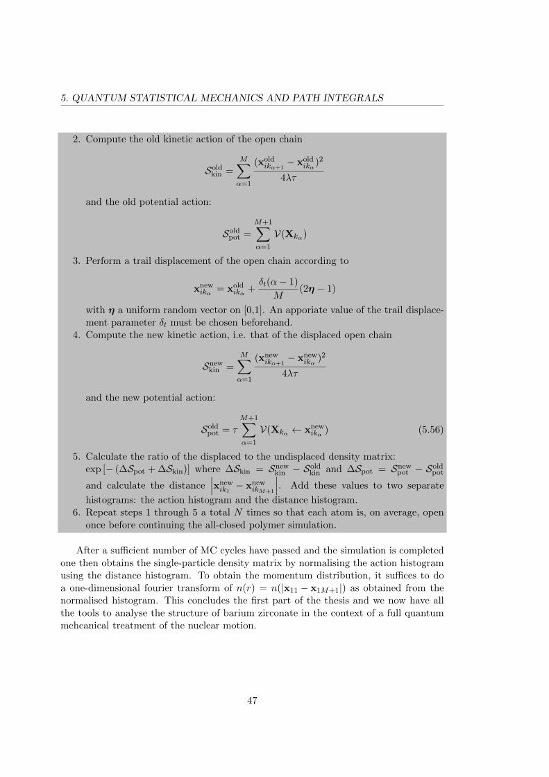
5. QUANTUM STATISTICAL MECHANICS AND PATH INTEGRALS
2. Compute the old kinetic action of the open chain
Soldkin =
M∑α=1
(xoldikα+1
− xoldikα
)2
4λτ
and the old potential action:
Soldpot =
M+1∑α=1
V(Xkα)
3. Perform a trail displacement of the open chain according to
xnewikα = xold
ikα +δt(α− 1)
M(2η − 1)
with η a uniform random vector on [0,1]. An apporiate value of the trail displace-ment parameter δt must be chosen beforehand.
4. Compute the new kinetic action, i.e. that of the displaced open chain
Snewkin =
M∑α=1
(xnewikα+1
− xnewikα
)2
4λτ
and the new potential action:
Soldpot = τ
M+1∑α=1
V(Xkα ← xnewikα ) (5.56)
5. Calculate the ratio of the displaced to the undisplaced density matrix:exp [− (∆Spot + ∆Skin)] where ∆Skin = Snew
kin − Soldkin and ∆Spot = Snew
pot − Soldpot
and calculate the distance∣∣∣xnewik1− xnew
ikM+1
∣∣∣. Add these values to two separate
histograms: the action histogram and the distance histogram.6. Repeat steps 1 through 5 a total N times so that each atom is, on average, open
once before continuing the all-closed polymer simulation.
After a sufficient number of MC cycles have passed and the simulation is completedone then obtains the single-particle density matrix by normalising the action histogramusing the distance histogram. To obtain the momentum distribution, it suffices to doa one-dimensional fourier transform of n(r) = n(|x11 − x1M+1|) as obtained from thenormalised histogram. This concludes the first part of the thesis and we now have allthe tools to analyse the structure of barium zirconate in the context of a full quantummehcanical treatment of the nuclear motion.
47

CHAPTER 6
RESULTS
In this chapter we will present the results of our simulations, focusing on pair correlationfunctions and momentum distributions for the BaZrO3 system. The first part of thischapter, however, will be dedicated to verifying that all the algorithms that have beenimplemented are working properly.
The source code for all our programs can be found in appendix B, here we will onlyprovide a brief summary of the most important component programs needed to performa PIMC simulation:
• InitialiseLattice.f90: Initialises the system. A BaZrO3 supercell of a specifieddimension is created and the atoms are placed in their equilibrium configuration.Arrays containing atomic type, charge and mass are also created.• Potential.f90: Calculates the total interaction energy of a single atom in the
field of all the other atoms. Note that this includes both the Buckingham po-tential which we described how to calculate thoroughly in Section 3.4 and theEwald summation which was the topic of Section 3.5. For more details on how toimplement the Ewald summation the reader is referred to appendices A and B.• Metropolis.f90: Implements the PIMC method as described in Section 5.5. For
the sampling of new paths we have implemented both single slice sampling as wellas the bisection method (which is available in separate version of the Metropolisprogram). Note that both versions use COM moves to help find AFD configura-tions.• OpenChain.f90: Implements the open chain algorithm as described in Section 5.9.
Note that this program is very similar to the regular PIMC program, the exceptionbeing that one polymer chain is now open and diagonal properties cannot becalculated.• PairCorrelation.f90: Used in conjunction with the Metropolis.f90 subroutine
to calculate the pair correlation function.• EnergyEstimator.f90: Implements the thermodynamic estimator for the internal
48

6. RESULTS
energy, see Eq. (5.40). Used in conjunction with the Metropolis.f90 subroutine.• TrailMethod.f90: Implements the Trail method for calculating the single particle
density matrix, see Section 5.9.2.
Some minor subroutines for writing data etc. have not been listed above. All post-processing of the simulation data has been carried out in MATLAB.
6.1 Verification part I: The potential
A good starting point is to verify the program responsible for calculating the potentiali.e. both the short-range interaction given by the Bucking potential in Section 3.2 as wellas the long-range coulomb interaction given by the Ewald summation in Section 3.5. Asa first step to verifying that our program is calculating the potential correctly we will useit to calculate the equilibrium lattice constant for the BaZrO3 system. For this purposewe will use the original set of parameters listed in Table 3.1, which have been reportedto give an equilibrium lattice constant a0 = 4.188 A [4]. To test whether our programcan reproduce this value we will use a simple method: Several BaZrO3 supercells areinitialised using different lattice parameters with values in a suitable interval. For eachvalue of the lattice parameter we calculate the total interaction energy of the system,the correct equilibrium lattice paramter is then the value for which the total interactionenergy is a minimum. The resulting curve is displayed in Fig. 6.1 where the interactionenergy per unit cell is plotted as a function of the lattice parameter a0.
Clearly from Fig. 6.1 the minimum in energy occurs somewhere in the vicinity ofa0 ≈ 4.2 A and by doing a careful scan with a small step around that value we find thatthe exact equilibrium lattice constant is a0 = 4.188 A in agreement with the value foundin [4].
As a further check for the coulombic interaction and the implementation of the Ewaldsummation one can compute the Madelung constant which is a dimensionless value thatdepends only on the lattice structure and ionic charges and has been well documentedfor nearly all of the commonly occuring lattice types. Consider a lattice with N ions, inSI units the total electrostatic potential felt by an ion i in the field of the N − 1 otherions is given by
Φi =e
4πε0
∑j 6=i
Zjrij
(6.1)
where rij = |xi − xj | is the distance between atoms i and j and Zj is the numberof elementary charges on ion j. If we denote by d the nearest neighbour distance in thelattice the Madelung constant can be defined as
Mi =∑j 6=i
Zjrij/d
. (6.2)
We can then write electrostatic potential Φi = e4πε0
Mid and the corresponding elec-
trostatic energy is
49

6.1. VERIFICATION PART I: THE POTENTIAL
2 4 6 8 10
−140
−120
−100
−80
−60
−40
Lattice constant a0 (Å)
Tot
al in
tera
ctio
n en
ergy
/ un
it ce
ll [e
V]
Total interaction energy as a function of lattice constant
Figure 6.1. The total interaction energy per unit cell as a function of lattice parameter a0 fora 4×4×4 BaZrO3 supercell.
Vi =e2
4πε0
Mi
d. (6.3)
The number of Madelung constants associated with a particular crystal structuredepends on the number of different ions and the crystal symmetry. For BaZrO3 we arelooking at three different values: MBa, MZr and MO. These three different constantscan be combined to form a single, effective Madelung constant proportional to the totalelectrostatic energy of one BaZrO3 formula unit. We define this effective Madelungconstant 1 as
Meff =1
2(ZBaMBa + ZZrMZr + 3ZOMO) =
1
2(2MBa + 4MZr − 6MO) (6.4)
and consequently the total electrostatic energy per unit formula is Vformula = Meffe2
d .Now, we can easily calculate MBa, MZr and MO using our Potential.f90 subroutine ifwe temporarily neglect all the contributions from the short-range Buckingham potential.The program can then output the pure electrostatic energy felt an arbitrary ion in thefield of all the other ions and it is then a small matter to compute Meff from Eq. (6.4)since e.g. MBa = VBa
4πε0de2
. We find that
1In litterature this is often just plainly referred to as the Madelung constant
50

6. RESULTS
Meff = −24.7549 (6.5)
which is in good agreement with e.g. the value Meff = −24.7550 reported in [6].All calculations presented in this section were performed on a 4×4×4 BaZrO3 supercellcontaining a total of 320 ions. For the Buckingham potential a raidial cut-off rcut = 6 Awas used while for the Ewald summation the tolerance was set to ε = 10−7. We notebriefly that this tolerance factor is approximately an upper bound for the error and thevalues for the radial cut-offs in real and reciprocal space mentioned in Section 3.5 arethen determined by ε. For a more detailed discussion of parameters used in the Ewaldsummation the reader is referred to appendix A.
In conclusion, our program for calculating potential accurately reproduces the knownvalues of both the equlibrium lattice constant for BaZrO3 as well as the Madelungconstant for a perovskite structure system and proceed, reasonably condifident that theprogram is working as intended.
6.2 Model potentials and antiferrodistortive instabilities
We saw in Chapter 2 that in many perovskite structured oxides there are antiferrodis-tortive phases where the oxygen octahedra are tilted and where the tilting may be out-of-phase between neighbouring octahedron in one or more of the x,y and z-directions.The energy difference between these phases and the cubic strucutre is usually very small.In the case of BaZrO3 it was also mentioned that calculations have given no conclusiveindications as to whether such antiferrodistortive instabilites can be found or if the ma-terial remains cubic all the way down to T = 0. While we do not attempt to solve thisissue in this thesis, what we have done is create two sets of Buckingham pair potentialparameters for barium zirconate where one set describes a system with AFD instabilitieswhile the other set given a cubic system and the purpose of this section is to show howthis was done. In Chapter 2 Section 2.2 we briefly described a steric model which partlyexplains the origins of the octahedral tilting and saw that instabilities are related to theGoldschmidt ratio which in turn depends on the ionic radii. In this model tilting occursbecause of a mismatch in size between the A and B cations in a perovskite. In the rigid-ion model with a Buckingham potential, the relative ionic radii are partly determinedby the ρ parameters found in the exponential Pauli repulsion term:
V(r) = Ae− rρ − C
r6. (6.6)
This suggests that in order to go from a stable system to an unstable one or vice versaone can simply change the relative magnitudes of the ρ parameters for the Ba-O andthe Zr-O interactions (while leaving the other parameters unchanged). A good startingpoint is to first investigate the original set of parameters values by Stokes and Islamgiven in Table 3.1 by looking at the phonon spectrum as mentioned in Section 2.2. Thefollowing analysis and results were kindly contributed by E. Fransson and J. Hakansson[16] who have calculated phonon spectra and analysed the resulting eigenmodes for
51

6.2. MODEL POTENTIALS AND ANTIFERRODISTORTIVE INSTABILITIES
different sets of parameters (ρBa-O,ρZr-O). For the Stokes values ρBa-O = 0.3949 A−1
and
ρZr-O = 0.3760 A−1
the resulting phonon spectrum is displayed in Fig. 6.2.
X M R M−5
0
5
10
15
20
25
30
Γ Γ Γ
Fre
quen
cy [T
Hz]
Figure 6.2. Phonon spectrum for the pair potential described in Chapter 3. Phonon modefrequencies are displayed along lines of high symmetry in the brillouin zone. Note thatthere are no soft modes with imaginary frequency present indicating that the system isstable and will remain cubic.
Here, the phonon mode frequencies are plotted along the usual high symmetry linesof the brillouin zone. Imaginary frequencies are represented as negative values in thisfigure but as we can see such soft phonon modes are absent, indicating that the crys-tal is stable. This leads us to conclude that the set of parameters determined for theBuckingham potential by Stokes and Islam yields a BaZrO3 system without AFD in-
stabilites. However, changing the size of the parameters to ρBa-O = 0.3820 A−1
and
ρZr-O = 0.3885 A−1
, which corresponds to a decrease in the Goldschmidt ratio, resultsin a quite different phonon spectrum shown in Fig. 6.3.
Observe the prescene of imaginary R- and M -point frequencies in Fig. 6.3 whichare indicative of phase transistions that lowers the crystal symmetry. An analysis ofthe polarisation vectors revealed displacements corresponding to four different unstablemodes: three R-point modes specified in glazer notation as a0b−b−, a−b−b−, a−a−a−
and one M -point mode a0a0c+. However, as it turns out, only AFD phases with a−a−a−
tilts are actually observed during simulations and therefore we shall focus on this typeof tilt. The absence of AFD phases with tilts specified by a0b−b−, a−b−b− and a0a0c+
is related to the depth and location of the energy minima as a function of rotation anglefor the tilted structures, see Fig. 6.4 for an example of such a curve. Henceforth, weshall refer to the orginal set of parameters as the cubic system since in this case there
52

6. RESULTS
X M R M−5
0
5
10
15
20
25
30
Γ Γ Γ
Fre
quen
cy [T
Hz]
Figure 6.3. Phonon spectrum for the pair potential with new values of ρBa-O and ρZr-Odescribed above. This time there are soft phonon modes with imaginary frequency indicatinga possible phase transition where the crystal symmetry is lowered.
are no AFD instabilities according to Fig. 6.2 while the new set of parameters shall bereferred to as the tilt system. For the sake of clarity we summarise these two modelpotentials below:
1. The cubic system: Uses the original set of Buckingham potential parametersfound in Table 3.1 which yields a cubic system.
2. The tilt system: Uses the same parameters as the cubic system except for the
values of ρBa-O and ρZr-O which are changed to ρBa-O = 0.3820 A−1
and ρZr-O =
0.3885 A−1
. This system has AFD phases where the oxgen octahedra exhibita−a−a− tilts.
Naturally, one also would like to know how close the unstable tilt system is tothe original cubic structure in energy. This is easy to caculate since we already havea program for calculating the total energy of the system, meaning we only have torotate the octhedra to establish a a−a−a− tilt and then record the difference in energybetween the tilted and the original structure. These calculations have been carried outfor different octahedral rotation angles in a small range and are displayed in Fig. 6.4.Since two neighbouring octahedra share a common oxygen atom, the tilting is not trulya rigid rotation but involves a small amount of distortion. Therefore, we have chosen asmall displacement parameter ∆ to characterise the magnitude of the tilt meaning eachoxygen atom in an octahedron is displaced an amount ∆ along a straight line in thedirection necessary to establish an overall a−a−a−-tilt. Keep in mind that changing the
53

6.2. MODEL POTENTIALS AND ANTIFERRODISTORTIVE INSTABILITIES
parameters in the potential also changes the equilibrium lattice constant and for the newtilt system we find that a0 = 4.255 A. Since the lattice constant and other propertieshave now changed slightly, one could think of this new model potential as describingsome other cubic perovskite closely related to barium zirconate. The important point isthat in this system, which still highly resembles the old one, there are now AFD phases.
0 0.05 0.1 0.15 0.20
50
100
150
200
250
300
Displacement ∆ (Å)
Ene
rgy
diffe
renc
e / u
nit c
ell (
meV
)
Energy difference between the a−a−a− AFD and the undistorted phase
0 0.05 0.1 0.15 0.2−10
−5
0
5
10
Tilt systemCubic system
Figure 6.4. The difference in energy between undistorted and AFD phases for the two modelpotentials as a function of the displacement parameter ∆ which determines the magnitude ofthe tilt. Note that energy increases for the cubic potential as expected while for the unstablepotential the system can decrease its energy by tilting the octahedra. In glazer notation thistilt is represented by a−a−a−.
From Fig. 6.4 it is apparent that tilting the octahedra increases the energy in thecase of the cubic system while the energy is lowered for the tilt system as expected. Byinspecting the rightmost figure we see that the maximum in energy difference betweenthe AFD and undistorted phase for the tilt system occurs at approximately ∆ = 0.13 Awhere energy for the AFD phase is lower by an amount ∆E ≈ −7.4 meV per unit cell.Clearly this is a relatively small energy difference and it is not evident that quantumfluctuations can be neglected.
Identical curves to those in Fig. 6.4 can be computed for the a0b−b−, a−b−b− anda0a0c+ tilt modes and it is found that the minima in energy difference between thecubic and distorted strucutures are more shallow for these types of tilt and occur atlarger values of ∆. As a consequence, only a−a−a− AFD phases are actually observed.Note that geometrically, an a−a−a− mode corresponds to a rotation of the octahedraabout an axis ω = (1, 1, 1) through the zirconium atom. This rotation axis is onlyunique up to a sign however, and consequently there are eight different possibilitiesω = (±1,±1,±1). For each oxygen ion there are thus several equivalent sites which
54

6. RESULTS
are separated by energy barriers. Thermal crossings of these barriers are possible atnon-zero temperatures but as the temperature tends towards zero the oxygen ions willget stuck in one of the sites so that in the ground state an a−a−a− tilt with a definiteaxis of rotation ω is established. Naturally, there is an equal probability to find eachone of the eigth rotations ω = (±1,±1,±1) in the ground state. On the other handat sufficiently high temperatures, the oxygen ions can move freely between the differentsites and the resulting system looks on average cubic [16]. These equivalent sites forthe oxygen atom in the tilt system will be important when we study the momentumdistribution later on.
6.3 Verification part II: The Path Integral Monte-Carlomethod
In Section 6.1 we verified that the potential is evaluated correctly by our program andsimilarily, we now verify the implementation of the PIMC method as described in Sec-tion 5.5. A convenient way to verify a large part of the program is to study a quantumharmonic oscillator with no external driving forces. In this particularily simple caseone can derive an exact solution for the internal energy of the system as a function oftemperature and we can then check to see whether our program reproduces this value.In particular, we compare the energies obtained by the different methods for samplingthe paths introduced in Chapter 5 Sections 5.5 and 5.7. In addition, to validate the im-plementations of the open chain method and the trail method introduced in Section 5.9we compare the distributions obtained to the analytic expression for the ground stateposition distribution.
Consider a single, one-dimensional quantum mechanical harmonic oscillator (QHO).The potential has the familiar quadratic form
V(x) =1
2mω2x2 (6.7)
where m is the mass and ω is the angular frequency. Recalling Section 5.2 we can,with a bit of algebra, evaluate the partition function
Z = tr(e−βH
)=
∫dx〈x|eβH|x〉 =
e−β~ω2
1− e−β~ω. (6.8)
The internal energy is given by Eq. (5.9):
E = 〈H〉 = − ∂
∂βln(Z) =
~ω2
coth
(β~ω
2
). (6.9)
From Eq. (6.9) we can evaluate the energy for a given angular frequency and tem-perarature. To make things simple we work in the natural units of the oscillator~ = λ = kB = 1 and in addition we set the oscillator angular frequency ω = 1. ForT = 0.1 K we find from Eq. (6.9) that E = 0.5000 K and expect to be able to reproduce
55

6.3. VERIFICATION PART II: THE PATH INTEGRAL MONTE-CARLOMETHOD
this value in a PIMC simulation using the thermodynamic estimator Eq. (5.40) to com-pute the energy. A few minor modifications to the collection of subroutines describedin the introduction to this chapter are necessary: one has to write a new subroutine forcalculating the potential, but this is trivial given the simple harmonic form Eq. (6.7) andfurthermore there is no need to use any periodic boundary conditions. To intialise theoscillator path we set x = 0 for each bead. This is also a good opportunity to comparethe performance of the simple single slice sampling technique introduced in Section 5.5to the more advanced bisection algorithm described in Section 5.7.2. As discussed inSections 5.5, the number of beads M controls how well quantum mechanical effects areapproximated in the simulation. A value M = 1 corresponds to a classical MMC sim-ulation and higher values of M will yield increasingly better approximations. Thus,to reproduce the theoretical value E = 0.5000 K it is essential that enough beads areincluded. To ensure this we calculate the energy for a wide range of M values and checkhow many beads are necessary to reach an asymptotic value. Fig. 6.5 shows a compar-ison of the energy at T = 0.1 K as a function of the number of beads calculated usingsingle slice and bisection sampling, respectively. In generating this figure all the PIMCsimulations were allowed to run until the estimated MC error2 was less than 1× 10⁻⁴.
From Fig. 6.5 it is immediately apparent that for values of roughly M > 50 an asymp-totic value very close to the theoretical value E = 0.5000 K can be obtained equally wellusing either sampling technique. Indeed, the figure suggests that in terms of the num-ber of beads required for convergence, sampling new paths using the bisection algorithmoffers no advantage over single slice sampling. This is to be expected since regardlessof the sampling technique we are still working within the primitive approximations andreducing the number of beads needed can only be achieved using a higher-order actionapproximation. Instead, to reveal the difference in performance between the two sam-pling techniques we will look at the time required for an individual PIMC simulationto converge with an MC error less than 1× 10⁻⁴ as a function of the number of beads,Fig. 6.6. Here it becomes clear that the bisection algorithm vastly outperforms singleslice sampling when it comes to the rate with which phase space is explored, e.g. usingM = 100 beads the PIMC simulation using bisection sampling only takes approximatelyone third of the time required using single slice sampling3.
This is the desired result since the whole reason for introducing the bisection algo-rithm was to improve the sampling of new paths. Also keep in mind that this is justa model system for which evaluating the potential is relatively cheap, for a real sys-tem such as the barium zirconate system we will study in the upcoming sections, usingbisection sampling can significantly reduce the simulation time. In conclusion, the im-plementation of the PIMC algorithm gives satisfactory results for a QHO model systemand we have also shown that the sampling can be improved by a considerable amountusing the bisection algorithm.
Our next task is to verify the algorithms used to calculate the momentum distri-
2Calculated using the relations introduced at the end of Section 4.2, including an estimate of thestatistical inefficiency.
3These exact numbers depends, of course, on the system and implementation but the trend is quiteclear.
56

6. RESULTS
0 50 100 150 2000.4
0.45
0.5
0.55
Number of beads M
Ene
rgy
(K)
QHO internal energy
Single sliceBisection
Figure 6.5. The internal energy for a quantum harmonic oscillator system as a function ofthe number of beads M used in the PIMC simulation. Two sets of data are shown, the bluecircles show the results obtained using the bisection algorithm to sample new paths whilethe red crosses show the corresponding results using single slice sampling. Observe that theperformance of the two sampling methods in this case is identical and an symptotic valueof the energy is attained for roughly M > 50.
bution. Recall from Section 5.8 that the momentum distribution can be obtained asthe fourier transform of the single particle density matrix or equivalently the end-to-enddistance distribution. This can be calculated using either the open chain method or thetrail method, both described in Section 5.9. A suitable test is to compare the distribu-tion obtained using these two methods to the QHO ground state position distributionif we perform our calculations at a low temperature so that mainly the ground state ispopulated. Fig. 6.7 shows the position distributions obtained for T = 0.1 K using thetwo different methods with M = 100 beads. The analytical predictions are displayedin the same figure and we can see that both methods produce distributions that agreefarily well with analytical prediction. Comparing the performance of the two methodsthe open chain algorithm converged significantly faster, within the span of a few minuteson an average desktop computer compared to the trail method which took several hours.
6.4 Barium Zirconate
In Section 6.2 we established two model potentials for BaZrO3, both based on a Buck-ingham potential for the short-range interaction and the Ewald summation for the long-
57

6.4. BARIUM ZIRCONATE
0 50 100 150 2000
10
20
30
40
50
60
70
Number of beads M
Simulation time required for convergence
Tim
e (m
inut
es)
Single sliceBisection
Figure 6.6. The time required in order to converge the internal energy of a QHO with anerror better than 1× 10⁻⁴ as a function of the number of beads used. Blue circles show thetimes measured using the bisection algorithm to sample new path while the red crosses arethe corresponding times obtained using single slice sampling. Here we note that bisectionsampling yields a much better rate of convergence and that the discrepancy between the twomethods grows with the number of beads.
range electrostatic interaction. The first model potential describes a system withoutAFD instabilities i.e. is always cubic while the other potential describes a tilt systemwhere there are AFD phases. The purpose of this section is to show the results from cal-culations of pair correlation functions, momentum distribution and the internal energy.These calculations have been performed for both model potentials and comparing theresults will enable us to see the impact of the AFD instabilites when nuclear quantumeffects are taken into account. In the first section, we look at the internal energy of thesystem which is an important property in itself but here we will mainly use it as a meansof studying equilibration and convergence. The pair correlation function is treated inthe following section providing a nice visualisation of the quantum fluctuations. The lastpart of this chapter deals with the single particle density matrix, momentum distributionand algortihms used for their calculation.
6.4.1 Internal energy
The internal energy of the system can be calculated in a PIMC simulation using the ther-modynamic estimator described in Section 5.6. The difference from a classical MMC
58

6. RESULTS
0 1 2 3 4 5 6 7 80
0.05
0.1
0.15
0.2
0.25
0.3
0.35
0.4
R (QHO units)
n 0(R)
QHO ground state position distribution , M = 100
Analytical predictionOpen chain algorithmTrail method
Figure 6.7. Verification of the open chain algorithm and the trail method by comparing theend-to-end distance distributions obtained at T = 0.1 K to the ground state probabilitydistribution for the harmonic oscillator. From the figure it is observed that both algorithmsyield distributions in good agreement with the analytical prediction. The convergence ratefor the trail method turned out to be a lot slower.
simulation is the addition of a kinetic contribution from the springs coupling neighbour-ing beads. While the internal energy is an important property of the system we shall bemore interested in calculating the momentum distribution (see Section 6.4.3) and theenergy calculations will primarily be used as a tool to study the equilibration and con-vergence. In an ideal scenario one would determine a set of quantities to be calculatedand then perform a detailed convergence study for each of these properties, determiningthe number of PIMC cycles as well as the number of beads required to obtain convergedresults. In this work we are more interested in the qualitative behvaiour of the systemhowever, and will adopt a less rigorous approach when checking for convergence.
To get an idea of how long the system needs to equilibrate we can look at the totalenergy for each generated configuration, i.e. the expression inside the angular bracketsin Eq. (5.40), as a function of the number of PIMC cycles. Such a plot is displayed inFig. 6.8 where the energy for each newly generated configuration of a BaZrO3 system isrecorded at T = 30 K.
From Fig. 6.8 a rapid initial increase in energy is observed during the first 50 PIMCcycles after which the curve becomes more even and the energy starts to fluctuate arounda mean value. This behaviour makes sense since the system was initialised in the T = 0 Kequilibrium configuration. From Fig. 6.8 it can be discerned that the thermalisationperiod is somewhere around 50 PIMC cycles in this case and it is good practice to
59

6.4. BARIUM ZIRCONATE
0 100 200 300 400 500−141.88
−141.86
−141.84
−141.82
−141.8
−141.78
−141.76
−141.74
Number of MC cycles
Ene
rgy
/ uni
t cel
l (eV
)Internal energy at T = 30 K, M = 20
Figure 6.8. Equilibration in a PIMC simulation of BaZrO3. Initially all the beads are in theT = 0 K equilibrium configuration but as the simulation proceeds the internal energy of thegenerated configurations starts to increase and after roughly 50 PIMC cycles the energy ofthe configurations stabilises and starts to fluctuate.
let the actual equilibration period Neq extend over a number of steps corresponding toa few multiples of this thermalisation time. Thus we will always use at least Neq =200 equilibration cycles when attempting to calculate any property of the system. Anexception occurs if we do a so called warm start where the initial distribution is nolonger the T = 0 K configuration but rather some configurations stored from a previousrun. If the conditions were similar during this preliminary run we can afford to use ashorter equilibration period. This will be the case when calculating properties for thetilt system.
We will now look at the internal energy as a function of the number of beads M used.Since increasing the number of beads used in a simulation quickly becomes expensive oneshould do a convergence study to determine how many beads are required to reach anasymptotic value, much like we did in the previous section with the QHO. Fig. 6.9 showsthe internal energy for a 2×2×2 BaZrO3 system for a few different values of M and attwo different temperatures. In creating this figure, all the simulations were allowed torun until the estimated MC error was smaller than 1× 10⁻⁴.
We observe that at T = 30 K, increasing the number of beads yields a steadilyincreasing energy from M = 1 to somewhere around M = 25 where an asymptotic valuehas been obtained. Thus we can conclude that at this particular temperature, if weare interested in the internal energy of the system, choosing 20 < M < 30 would be asuitable compromise between accuracy and computational efficiency. As the temperatureincreases the expectation is that fewer beads will be required since quantum effects will
60

6. RESULTS
0 5 10 15 20 25 30−141.9
−141.85
−141.8
−141.75
−141.7
−141.65
−141.6
Number of beads M
Ene
rgy
/ uni
t cel
l (eV
)
Energy as a function of the number of beads
T = 30 K
T = 150 K
Figure 6.9. Comparing the internal energy of a 2×2×2 BaZrO3 for several different valuesof the number of beads M and at two different temperatures. For the lower temperatureT = 30 K at least 20 beads are required to get close to an asymptotic value while at a highertemperature T = 150 K we could get away with using only M ≈ 5 beads.
not be as important. This is indeed the case looking at the T = 150 K measurementswhere increasing the number of beads beyond M = 5 does not significantly changethe value of the internal energy. Hence, in this case we could get away with using asmaller number of beads compared to the low temperature case. Since we are mostlyinterested in qualitative behaviour, we will restrict ourselves to M = 20 beads whencalculating the pair correlation function and momentum distribution at T = 30 K in theupcoming sections. It should also be noted that the convergence with respect to thenumber of beads might look slightly different for the momentum distribution comparedto the energy. Ideally one would do a separate convergence study for the momentumdistribution but we shall take the number M = 20 on faith in order to save time.
6.4.2 The pair correlation function
The pair correlation function was defined in Section 4.5 and describes the distributionof atomic pairs in the system. For systems that are not monatomic, rather than lookingat g(r) for the entire system one defines fractional pair correlations where each possibletype of two-atom combination that can be formed is described by a separate correlationfunction. For a BaZrO3 system there are four possibilites: Ba-O, Zr-O, Ba-Zr andO-O. Out of these four types of pairs we are only really interested in the distribution forpairs of oxygen atoms since these are the atoms which are displaced in an AFD phase,see Chapter 2. In this section we will look at pair correlation functions calculated for
61

6.4. BARIUM ZIRCONATE
the two different model systems described in Section 6.2 using the estimator Eq. (5.41)defined in Section 5.6 . All calculations presented here were performed on a 4×4×4BaZrO3 supercell using a radial cut-off rcut = 8 A for the Buckingham potential and theewald error parameter ε = 1 × 10⁻⁷. Fig. 6.10 shows how the pair correlation functionfor the cubic system using M = 20 and M = 1 beads respectively, included are also theexpected δ-function peaks for the T = 0 K structure.
0 2 4 6 8 100
2
4
6
8
10
12
14
16
18
r (Å)
g(r)
O−O Pair correlation function at T = 30 K, cubic system
PIMCClassical MMCT = 0 K Peaks
Figure 6.10. Oxygen-Oxygen pair correlation function for a BaZrO3 supercell system. Threedifferent sets of data are shown, the red curve corresponds to a PIMC simulation with M = 1which equivalent to a classical MMC simulation while the blue curve shows the results froma PIMC simulation with M = 20. Finally, the dotted grey lines shows the expected peaksfor the T = 0 K configuration. When quantum effects are taken into account we see thatthe delocalisation in the system increases since the blue distribution is wider.
Note that since using M = 1 beads reduces the PIMC method to the classical MMCmethod we can observe a purely thermal broadening of the peaks compared to theT = 0 K case. When M 6= 1 however, there is an addition to the width of the peaks dueto quantum delocalisation. Note that in order for the quantum effects to appear thetemperature needs to be low enough and we have found that T = 30 K is sufficiently lowthat quantum delocalisation can be observed as evidenced by Fig. 6.10. The situationbecomes more interesting looking at the tilt system, here we expect the oxygen ions tofind alternative configurations corresponding to tilted octahedra given that the temper-ature is low enough that the difference between alternate sites for the oxygen ions arenot erased by thermal fluctuations. Fig. 6.11 shows the O-O pair correlation functioncalculated for the tilt system with M = 1 and M = 20 respectively.
Comparing the classical M = 1 case here to the corresponding curve in Fig. 6.10 it isclear that there exist additional peaks in the tilt system corresponding to the positions
62

6. RESULTS
0 2 4 6 8 100
5
10
15
r (Å)
g(r)
O−O Pair correlation function at T = 30 K, tilt system
PIMC
Classical MMC
Figure 6.11. Oxygen-Oxygen pair correlation function for a BaZrO3 supercell system withAFD instabilities. We note the appearance of alternative peaks corresponding to rotatedoctahedra in this figure. When quantum effects are taken into account the alternative peaksare partly erased as seen by comparing the classical result (orange) to the PIMC result(blue).
occupied by oxygen pairs in a system with rotated octahedra. When we take quantumfluctuations into account however, delocalisation partly erases some of these additionalpeaks or make them less distinguished as evident from the M = 20 correlation functionin Fig. 6.11. A crucial component in obtaining this figure was to do a warm start whereafter running an initial simulation with M = 1 during which system was allowed tothermalise and then find the alternate configurations corresponding to tilted octahedra,the resulting configuration was saved and used to restart a simulation with M = 20beads.
6.4.3 The momentum distribution
The pair correlation function gives information about the structure of the system but ifone is interested in the impact of nuclear quantum effects one needs to study the singleparticle density matrix (or rather end-to-end distance distribution which is what oneactually calculates) and the momentum distribution. These were defined in Section 5.8and we also provided algorithms for their calculation in Section 5.9. We have alreadyseen an example of a end-to-end distance distribution for the simple case of a harmonicoscillator in Section 6.3. For a real system such as a BaZrO3 supercell, calculating themomentum distribution is computationally more demanding and the situation is furthercomplicated by the long-range Coulomb interaction and the prescence of AFD phases. Inparticular, during our calculations we were unable to obtain converged results for BaZrO3
using the trail method (see Section 7.2.2 for an expanded discussion of this result) and
63
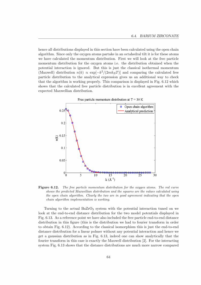
6.4. BARIUM ZIRCONATE
hence all distributions displayed in this section have been calculated using the open chainalgorithm. Since only the oxygen atoms partake in an octahedral tilt it is for these atomswe have calculated the momentum distribution. First we will look at the free particlemomentum distribution for the oxygen atoms i.e. the distribution obtained when thepotential interaction is ignored. But this is just the classical isothermal momentum(Maxwell) distribution n(k) ∝ exp[−k2/(2mkBT )] and comparing the calculated freeparticle distribution to the analytical expression gives us an additional way to checkthat the algorithm is working properly. This comparison is displayed in Fig. 6.12 whichshows that the calculated free particle distribution is in excellent agreement with theexpected Maxwellian distribution.
Figure 6.12. The free particle momentum distribution for the oxygen atoms. The red curveshows the predicted Maxwellian distribution and the squares are the values calculated usingthe open chain algorithm. Clearly the two are in good agreement indicating that the openchain algorithm implementation is working.
Turning to the actual BaZrO3 system with the potential interaction tuned on welook at the end-to-end distance distribution for the two model potentials displayed inFig. 6.13. As a reference point we have also included the free particle end-to-end distancedistribution in this figure (this is the distribution we had to fourier transform in orderto obtain Fig. 6.12). According to the classical isomorphism this is just the end-to-enddistance distribution for a linear polmer without any potential interaction and hence weget a gaussian distribution as in Fig. 6.13, indeed one can show analytically that thefourier transform in this case is exactly the Maxwell distribution [2]. For the interactingsystem Fig. 6.13 shows that the distance distributions are much more narrow compared
64

6. RESULTS
to the free particle distribution as expected. Furthermore we see that the distributionsfor the tilt and cubic systems respectively are fairly similar although the tilt systemdistribution is slightly wider.
0 0.2 0.4 0.6 0.8 1 1.2 1.40
0.5
1
1.5
2
2.5
3
r (Å)
n(r)
End−to−end distance distribution at T = 30 K, M = 20
Free particleTilt systemCubic system
Figure 6.13. The end-to-end distance distribution n(R) for oxygen atoms in barium zirconate.The plot shows a comparison between the distribution obtained for the cubic system and thecorresponding distribution for the tilt system. Evidently the two n(R) are very similar, thetilt system distribution being slightly wider at larger separations. As a reference point thefree particle end-to-end distribution is also dsiplayed, this distribution is gaussian as onewould expect for a linear polymer.
Unlike the pair correlation function, the convergence is very slow here, roughly150000 MC cycles were used to obtain Fig. 6.13, and in order to save time all cal-culations were performed on a 2×2×2 BaZrO3 supercell 4 but otherwise using the samesettings, including M = 20 beads and T = 30 K.
A complementary picture is provided by the momentum distribution, given by thefourier transform of n(R) as described in Section 5.8. Fig. 6.14 shows the momentum dis-tributions corresponding to the end-to-end distance distributions displayed in Fig. 6.13along with the free particle momentum distribution from Fig. 6.12. Compared to the freeparticle (classical) momentum distribution we can see that when quantum mechanics istaken into account the end result is a significantly wider distribution which, keeping theHeisenberg uncertainty principle in mind, we could already have guessed from Fig. 6.13.
From Fig. 6.14 we also note that the momentum distribution for the tilt system is
4Preliminary results indicate that the shape of the distribution is not overly sensitive to the systemsize but the purpose of this section is to provide a picture of the general behaviour rather than showingthe result of a long simulation with very small errors.
65

6.4. BARIUM ZIRCONATE
0 5 10 15 20 250
0.05
0.1
0.15
0.2
0.25
k (Å−1)
n(k)
Momentum distribution at T = 30 K, M = 20
Tilt System
Free particle
Cubic system
Figure 6.14. The momentum distribution n(k) for oxygen atoms in barium zirconate. Theplot shows a comparison between the cubic and the tilt system. We note that the two distri-butions are almost identical. As a reference point the free particle momentum distributionis also included and comparing the different curves we find that including quantum effectssignificantly alters the momentum distribution.
slightly more narrow than the corresponding distribution for the cubic system which alsomakes sense given Fig. 6.13 and the uncertainity principle. As discussed in Section 5.8 weshould look at the tails of the momentum distribution for indicators of nuclear quantumeffects. In particular, we are interested to see if there is a node in the tail of the tiltsystem momentum distribution. However, zooming in on the tails of the distributions inFig. 6.14 we end up with Fig. 6.15 from which it is evident that there are no observablenode in the tilt system distribution and indeed the two tails are almost identical.
66

6. RESULTS
18 20 22 24 26
−0.03
−0.02
−0.01
0
0.01
k (Å−1)
n(k)
Momentum distribution tails at T = 30 K, M = 20
Tilt systemCubic system
Figure 6.15. Zooming in on the momentum distribution tails from Fig. 6.14. Observe thatalthough there is a slight dip in the distributions there is no visible nodes and in particularthe two tails are almost identical.
67
CHAPTER 7
DISCUSSION
In this chapter we discuss the results presented in Chapter 6, the relative performanceof the different algorithms used and various other topics which have been touched upon.As previously noted, the purpose of this thesis has been twofold. One part consistedof showing how PIMC simulations can be used to calculate properties such as the mo-mentum distribution and what algorithms to use. The second part was to apply thesesimulation techniques to a BaZrO3 system for which we have established a simple model.Here, an important point was to obtain results for the two different model systems, onedescribing a cubic system and one describing a system with AFD instabilities, so thatthe two can be compared in the light of simulations where nuclear quantum effects aretaken into account. The reader should be aware that the main aim has been to obtainresults indicating general behaviour rather than conducting precise measurements ofquantities like the momentum distribution. As such, certain liberties have been takenin some cases, most notably the omission of proper error bars.
7.1 Inter-atomic interactions and the Ewald summation
The model used in this work combining the Buckingham potential and Ewald summationfor the electrostatic potential (see Chapter 3) is a standard one and only a few remarksare necessary. In defining the model potential we have used a rigid ion description inwhich the electrons are replaced by atomic net charges, van der Waals interaction andPauli repulsion. It is evident that this type of model cannot accurately describe e.g.polarisability. One way around this is to simulate the effects of having an electron cloudby using a shell model. Here, an atom is considered as consisting of both a core anda shell which are coupled by a harmonic spring [20]. Previous results have indicatedhowever that extending the model potential to include this interaction has very littleimpact on the kind of stuctural properties we are interested in here and to keep themodel simple we have chosen not to include such a shell model interaction.
Regarding the Ewald summation, summarised in Section 3.5 and investigated more
68

7. DISCUSSION
thorougly in appendix A, we note the existence of equivalent techniques for calculatingthe long-range interaction such as the particle-particle, particle mesh method (PPPM)[19]. Here one takes a quite different, more complicated approach to compute the elec-trostatic energy and is rewarded by a better overall scaling of O(N logN) rather thanO(N3/2) for the original Ewald summation 1 [19]. Generally speaking, there is a largerprefactor for the scaling in the case of PPPM however and one therefore only sees anincrease in efficiency for systems with a large number of particles. This motivated us tostick with the original Ewald summation method.
7.2 Simulation algorithms
We will now discuss the algorithms used in PIMC simulations. In particular, we areinterested in comparing the relative performance of the different options presented forsampling new paths and for calculating the momentum distribution.
7.2.1 The sampling of new paths
In Section 5.5 we described thoroughly the basic PIMC algorithm with single slice sam-pling i.e. where one bead is moved at a time akin to the classical MMC method. Theshortcomings of this method of sampling new paths were discussed in Section 5.7 wherewe also introduced two new types of moves in order to improve the sampling. The cen-tre of mass displacements (COM) described there have been used in practically all thesimulations performed to obtain the results presented in Chapter 6. It is important tonote that since this type of move consists of moving an atom as a whole, they have alimited impact on the convergence since quantum effects require relative displacementsbetween beads. Thus, COM moves must be carefully managed in the simulation andour strategy has been to perform one COM move every PIMC cycle (where one PIMCcycle consists of sampling on average a new path for each atom in the system i.e. inthe case of single slice sampling one MC cycle consists of one COM move plus randomlydisplacing NM beads). We have found that this gives a satisfactory convergence ratefor the properties of interest. However, when performing calculations on the tilt systemintroduced in Section 6.2 it was also discovered that if we limit the number of COMmoves to one every cycle, configurations with tilted octahedra are not found. This isnot suprising since a tilted configurations involves a collective displacement of severaloxygen atoms, incredibly unlikely to be achieved using single slice sampling. Ratherthan increasing the number of COM moves performed over the entire simulation, whichwould be ineffective in the long run, a better solution is to run a long simulation withM = 1 and then restarting the simulation with M = 20 from the resulting configuration.Using M = 1 the PIMC method reduces to the classical MMC method and finding con-figurations involving collective displacements of atoms is no longer a problem. This is auseful technique in general, especially for larger systems where the thermalisation can beaccelerated considerably by restarting the main simulation from an M = 1 simulation.
1Note that this scaling is only achieved if the parameters are chosen properly, see appendix A
69

7.2. SIMULATION ALGORITHMS
The second part of Section 5.7 treated bisection moves which can be used to replacethe single slice moves as a means of sampling new paths. Several previous investiga-tions have estblished the bisection method as superior [2] [3], a result that is echoedin Section 6.3 where we compared bisection sampling to single slice sampling by calcu-lating the internal energy for a harmonic oscillator and looking at the errorbars. Thisis certainly not suprising, given the careful construction of the bisection move. Oneof the main factors responsible for the increased convergence rate are that beads in apath are sampled directly from the free particle distribution and for the coarser levelsthis sampling is done at a higher temperature. This allows the beads to move largerdistances since the stiffness of the springs coupling neighbouring beads decreases withtemperautre. Another important point is that unlikely moves are rejected at the coarserlevels, removing the need to perform expensive calculations of the potential interactionat the finer levels and as a result we explore phase space faster. One notable drawbackof the bisection method is that it is hard to combine with the open chain method. Theorigin of the problem is in a sense technical, having an open chain severly limits thenumber of ways in which we can bisect it. As a consequence, for a fixed chain lengthand a fixed maxiumum bisection level, biases can arise where some beads are much morelikely to be sampled than others.
7.2.2 Calculating the momentum distribution
In Section 5.9 we described two different algorithms for calculating the momentum dis-tribution (or rather the end-to-end distance distribution which then has to be fouriertransformed in order to obtain the momentum distribution). The most straightforwardalgorithm is the open chain method which was derived by interpreting the defining equa-tion of the single particle density matrix in the language of the classical isomorphism.While the implementation is simple, we noted that one of the major disadvantages isthe fact that one cannot calculate diagonal properties in the same simulation. Anotheroption the trail method in which one performs an ordinary simulation with ring poly-mers which is halted after each MC cycle. During this pause, paths (belonging to theatom type for which we wish to calculate the momentum distribution) are cut open anddisplaced one at a time. To obtain n(r) one calculates the ratio of the density matrixof the now open chain to that of the previously closed chain. The occurences are addedto a histogram which then gives n(r) at the end of the simulation.
In Section 6.3 we verified both these methods by comparing the caculated n(R) for aharmonic oscillator at a low temperature to the analytical expression for the ground statesingle particle density matrix. Here it was found that both methods indeed yield thecorrect result but that the convergence was significantly slower using the trail method.While the open chain algorithm yielded a converged result within minutes the trailmethod needed several hours. The situation deteriorated even further when we lookedat the momentum distribution for the BaZrO3 system in Section 6.4.3. In this casethe open chain algorithm yielded acceptable results within the span of a dozen hours(corresponding to roughly 100000 MC cycles) while the trail method failed to convergecompletely under the time span for which it was allowed to run (3 days on a desktop
70

7. DISCUSSION
computer, corresponding to roughly 200000 MC cycles). In the case of the QHO wealso observed that the convergence of n(R) at large distances seemed to be the mosttroublesome. These result are in stark contrast to the performance reported by theinventors of the trail method [3] who reported an increase in the rate of convergenceusing the trail method with a reduced variance. Taking a closer look at their report itappears most of their testing was done on a liquid neon system which only has short-range interactions which are modelled by either a Lennard-Jones potential or the AzizHFD-C2 potential. Using the latter potential we were able to reproduce in a preliminarystudy, coming to the same conclusion that the trail method converges significantly fasterin this case. A possible explanation2 lies in the magnitude of the interactions. Sincethe ratio of density matrices required in the trail method varies exponentially with thedifference in action, large action differences may lead to an increased variance. Thisis certainly the case for the BaZrO3 system where small displacements can lead tolarge differences in action due to the coulomb interaction. For the QHO it depends onthe angular frequency ω, in our simulations we set ω = 1 which gives relatively largeactions. For either of the two systems, the difference is likely to be large at large Rwhich would explain the convergence difficulties encountered during the calculation ofn(R) in Section 6.3.
The recommended approach is thus to use the open chain method for systems whichinclude long-range interactions (ionic system) or strong external potential while the trailmethod is preferable for systems with short-range or weak interactions (noble gases,Lennard-Jones systems etc). The major drawback of using the open chain methodis that we can no longer use bisection sampling as explained in the previous section.However, for ionic systems, the accelerated convergence compared to the trail methodmore than compensates the use of a more crude sampling technique.
7.3 Properties of barium zirconate
Having dealt with the technical aspects of the PIMC algorithms we will now turn toanalysing the actual results obtained for the BaZrO3 system and presented in Section 6.2and Section 6.4.
The pair correlation functions displayed in Section 6.4.2 do not require much com-ment. The expected tendency of peaks to become broader as the temperature increasesis observed as well as a broadening due to quantum delocalisation when M 6= 1. Notethat these two different mechanisms for delocalisation are in a sense competeting, atlower temperatures quantum delocalisation dominates and the quantum corrected paircorrelation is thus quite different from the classical one.
7.3.1 The momentum distribution
We explained in Section 6.2 the tilt system has AFD phases where the tilt can be de-scribed as a−a−a− in glazer notation. Geometrically this corresponds to a rotation of
2Barring any subtle mistakes in the implementation that the author is not aware of.
71

7.4. OUTLOOK AND FUTURE PROSPECTS
the octahedra about an axis ω = (1, 1, 1) through the zirconium atom. This rotationaxis is only unique up to a sign however, and consequently there are eight degeneratedstructures ω = (±1,±1,±1). There are thus different sites for the oxygen atoms sep-arated by energy barriers, much like in the case of the double potential well that wasdiscussed in Section 5.8. It is observed that the oxygen atoms can move between theseconfigurations when they have enough energy to surmount the barrier but at lower tem-peratures they tend to get stuck in one of the sites. This begs the question of whetherthe oxygen atoms can simultaneously occupy two such sites which would be possibleif the energy barrier is so low that zero-point motion effectively erases it. To answerthis we compare the momentum distributions displayed in Fig. 6.14 since for the cubicsystem there can be no tilt and the oxygen atoms are confined to vibrate around theirequilibrium position. Looking at the momentum distributions calculated in Section 6.4.3there is indeed a slight narrowing of the momentum distribution in the tilt system whichcould be indicative of tunneling as has been suggested by many others, see e.g. [7]. Thisnarrowing is typically followed by a node in the tail of the momentum distribution how-ever, regardless of whether the lowest lying energy level is actually above or below thebarrier. Evidently from Fig. 6.15 no such node appears for the tilt system and indeedthe tails of the distributions for the two systems are more or less identical. A concernhere is that the error of the calculations could be quite large but as a preliminary con-clusion it seems unlikely that two sites can be occupied simultaneously by an oxygenatom. Given more time, an exhaustive investigation would preferably include a detailedconvergence study, momentum distributions for several temperatures both above andbelow T = 30 K and a larger system size.
7.4 Outlook and future prospects
There are many exciting prospects and possible ways to extend the work done in thisthesis. Most pressing however is the need to do more thorough investigations of themomentum distribution for a wide range of temperatures below and around the AFDtransition point. This would most likely require an MPI or OpenMP parallel implemen-tation of the programs used here in order to speed up the calculations by moving themonto a cluster. This would also include carefully checking that the erros are small enoughand that a sufficient number of beads are used. This would allow us to more conclusivelyrule out or confirm the role of nuclear quantum effects in regards to the transition toan antiferrodistortive state. Due to time limitations such a study could unfortunatelynot be presented here. There is also the question of trying to improve the open chainalgorithm for calculating the momentum distribution since the results presented hereindicate that the trail method might be unsuitable for strongly-interacting systems.Another possbility which has barely been mentioned in this thesis is to use path integralmolecular dynamics (PIMD) instead of the Monte Carlo approach described here. Itwould be interesting to study the advantages and disadvantages of such an approach fora strongly interacting real system such as barium zirconate.
Other prospects include exploring high-order action approximations such as the Li-
72

7. DISCUSSION
Broughton action which could help make the PIMC simulations more efficient. Again,due to time limitations we did not explore the many options here, it should also be notedthat many higher-order schemes require the forces to be known. This is not necessarily aproblem since analytical derivatives can be obtained directly from the Ewald summationand Buckingham potential. Moving forward one could also proceed, using the PIMCtoolbox, to look at different perovskites which exhibit not only AFD transitions but so-called ferrodistortive transitions as well. One would then have a large set of competingstructures and the interplay between these could possibly be affected by nuclear quantumeffects.
73

CHAPTER 8
CONCLUSIONS
Below we summarise briefly the topics covered in this thesis along with the most im-portant conclusions. To study the structure and dynamics of barium zirconate a rigidion model with a pair potential which is the sum of a Buckingham potential and theCoulomb potential can be employed. Analysing the phonon spectrum with respect tosoft phonon modes appearing as imaginary frequencies provides a method of testingwhether a certain set of values for the potential parameters give rise to a system withAFD instabilities. Using this strategy two model systems have been established one sta-ble cubic system and one which exhibits AFD phases which can be described in glazernotation as a−a−a−. The difference in energy between the configurations in the differ-ent phases is small, on the scale of milielectronvolts, allowing for the possbility that thestructure is influenced by nuclear quantum effects.
Path integral Monte Carlo is an effective method for obtaining quantum correctedproperties for a solid or a liquid. In particular, the momentum distribution which isof special interest since it works as a fingerprint for nuclear quantum effects can becalculated during a PIMC simulation. The degree of accuracy with which quantumeffects are included in a PIMC simulation is determined by the number of beads Mused. To determine a suitable value for M the internal energy of a BaZrO3 system wascalculated for different values of M . For temperatures around T = 30 K a value M = 20is sufficient to yield an approximately asymptotic value of the internal energy. If thetemperature is increased fewer beads are needed, indeed at T = 150 K five beads aresufficient. An illustration of the effect of quantum delocalisation in the system is given bythe pair correlation function. Here our calculation reveal that a quantum treatment atT = 30 K yields significantly wider peaks in the pair correlation function than expectedfrom corresponding classical calculations. This broadening of peaks due to quantumdelocalisation competes with thermal broadening where the latter dominates at highertemperatures.
The main property of interest for the BaZrO3 system is the momentum distribution.Here two distributions were calculated at T = 30 K, one for the cubic system and
74

8. CONCLUSIONS
one for the tilt system which has AFD instabilities. By comparing the momentumdistributions for these two systems we concluded that the distribution for the tilt systemis slightly more narrow. However, seeing as the difference was quite small and the tailsof the two distributions were otherwise identical i.e. no nodes were found in the tiltsystem distribution, we make the preliminary conclusion that there is no simultaneousoccupation of several equivalent sites for the oxygen ions.
Regarding the algorithms used for calculating the momentum distribution during aPIMC simulation we conclude that either the open chain algorithm or the trail methodmay be used. The advantage of the trail method is that properties diagonal in positionsspace can be calculated in the same simulation as the momentum distribution whichis not possible in the open chain algorithm where one polymer must be open duringthe simulation. It is also possible to combine the trail method with more advancedsampling methods such as the bisection algorithm which can dramatically increase therate with which phase space is explored. On the other hand, the convergence rate forthe trail method appears to be highly dependent on the strength of the interaction inthe system, the perfomance being significantly worse for strongly interacting systemssuch as BaZrO3. The open chain algorithm on the other hand can be used to calculatethe momentum distribution for any system but converges slower than the trail metodfor weakly interacting system.
As mentioned above the convergence rate of a PIMC simulation can be improved byintroducing more advanced techniques for sampling new paths. For this purpose we alsoimplemented an alternative version of the main PIMC program making use of the bisec-tion algorithm. By studying a simple harmonic oscillator model system the superiorityof the bisection algorithm over regular single slice sampling was established. In particu-lar, when calculating the internal energy of the oscillator it was found that simulationsusing the bisection based sampling converged approximately three times faster than thecorresponding single slice sampling simulations. The difference in performance was alsofound to increase with the number of beads used. Another measure which can be takento explore phase space more efficiently is centre of mass displacements which turnedout to be a necessary component to discover configurations with rotated octahedra inBaZrO3.
75


REFERENCES
[1] Allen, M. P. and Tildesley D. J. (1991) Computer Simulation of Liquids, OxfordUniversity Press.
[2] Ceperley, D. M. (1995) Path integrals in the theory of condensed helium, Rev. Mod.Phys. vol. 67, no 2, pp. 279-356.
[3] Brualla, L. M. (2002) Path integral Monte Carlo: Algorithms and applications toquantum liquids., http://www.tdx.cat/handle/10803/6577 (2014-05-03).
[4] Stokes, S. J. and Islam M. S. (2010) Defect chemistry and proton-dopant associationin BaZrO3 and BaPrO3 , Journal of Materials Chemistry, vol 20, no 30, pp. 6258-6264.
[5] Chandler, D. P (1987) Introduction to modern statistical mechanics, Oxford Uni-versity Press.
[6] Q. C. Johnson and D. H. Templeton (1961) Madelung Constants for Several Stuc-tures, Journal of Chemical Physics, vol 34, no 6, pp. 2004-2007.
[7] Morrone, J. A. et al (2009) Tunneling and delocalization effects in hydrogen bondedsystems: A study in position and momentum space The Journal of ChemicalPhysics, vol 130, no 20, 204511
[8] Engel, H. et al (2012) Momentum Distribution as a Fingerprint of Quantum Delo-calization in Enzymatic Reactions: Open-Chain Path-Integral Simulations of ModelSystems and the Hydride Transfer in Dihydrofolate Reductase, Journal of ChemicalTheory and Computation, vol 8, no 4, pp. 1223-1234.
[9] Lebedev, A. I. and Sluchinskaya, I. A. (2013) Combined first-principles and EX-AFS study of structural instability in BaZrO3, http://arxiv.org/abs/1304.6359(2014-05-03)
77

REFERENCES
[10] Akbarzadeh, A. R. et al (2005) Combined theoretical and experimental study of thelow-temperature properties of BaZrO3, Physical Review B, vol 72, no 20, 205104
[11] Reiter, G. F. et al (2002) Direct Observation of Tunneling in KDP using NeutronCompton Scattering, Physical Review Letters, vol 89, no 13, pp. 283-288.
[12] Momma, K. and Izumi, F. (2011) VESTA 3 for three-dimensional visualization ofcrystal, volumetric and morphology data, Journal of Applied Crystallography, vol44, no 6, pp. 1272-1276.
[13] Matsumoto, M. and Nishimura, T. (1998) Mersenne Twister: A 623-dimensionallyequidistributed uniform pseudorandom number generator ACM Trans. on Modelingand Computer Simulation, vol 8, no 1, pp. 3-30.
[14] Miller, A. (1999) Allan Millers Fortran Software,http://jblevins.org/mirror/amiller/mt19937.f90 (2014-05-03).
[15] Trotter, H. F. (1959), On the product of semi-groups of operators Proceedings ofthe American Mathematical Society, vol 10, no 4, pp. 545-551
[16] Fransson, E. Laurell Hakansson, J. (2014) Local and Global Ordering in BariumZirconate, a Model Potential Study
[17] Jedvik, E. (2014) Chemical expansion in perovskite structured oxides
[18] Perram, J. W. et al (1988) An algorithm for the simulation of condensed matterwhich grows as the N3/2 power of the number of particles Molecular Physics, vol65, no 4, pp. 875-893
[19] Gibbon, P. and Sutmann, G. (2002) Long-Range Interactions in Many-ParticleSimulation NIC series, vol 10, pp. 467-506
[20] Kiang, C. and Goddard III, W. A. (1992) Effective Hamiltonians for motions withdisparate time scales: The quantum shell model and the classical statistical shellmodel Journal of Chemical Physics, vol 98, no 2, pp. 1451-1457
78

Appendices
79

APPENDIX A
THE EWALD SUMMATION
In the following section we will present a formal derivation of the Ewald summationmethod for computing the total electrostatic (or Coulombic) interaction of a charge-neutral ionic system. We will also briefly discuss how to select appropriate values forthe various parameters. To keep things simple we will consider a cubic simulation boxwith side L, volume V and containing N ions. If we further assume periodic boundaryconditions, we saw in Chapter 3 that the potential can be written as a sum over thebasic simulation cell and all its periodic images, defined by translation vectors of the formn = L(nx,ny,nz) with ni ∈ Z. Thus, we may write (in atomic units) the electrostaticpotential at a point of observation x due to all the ions located at xj on the followingform
Φ(x) =∑n
N∑j=1
qj|x− xj + n|
(A.1)
where we implicitly assume that if x = xj for any j this term is excluded for n = 0.Evaluating this expression might look straightforward but since the terms only decayas 1/r we end up with a sum that is, in mathematical terms, conditionally convergentmeaning that the result will depend on the order in which the terms were added. To fixthis one can build up the sum in succesive shells surrounding the primary cell, forminga spherical arrangement. This will solve the issue of the sum not being convergent butthe rate of convergence will still be slow due to the 1/r-dependence. To remedy this wewill rewrite the potential at an ionic site xi as
Φ(xi) = Φ(xi) + Φr(xi) + Φk(xi)− Φs (A.2)
Where the terms Φ(xi)+Φr(xi) and Φk(xi) correspond to sums in real- and reciprocalspace respectively which both converge very rapidly and Φs is a constant. This expansionis easy to understand from a physical viewpoint, the term Φr comes from an imaginedset of smeared charges centered on the ionic sites, where the total charge of each of the
81

smeared charges is equal to the corresponding ionic charge but with the sign reversed.The potential contribution from these smeared charges is then Φr. To compensate foradding this to Φ in Eq. (A.2) we must then add the contribution from a new set ofsmeared charges, this time with the same sign as their corresponding ions. Expandingthis contribution in reciprocal space and compensating for a self-interaction term yieldsthe last two terms Φk(x) and Φs. Clearly, the equality in Eq. (A.2) must then hold sinceall we have done is add potential contributions from two sets of smeared charges withopposite sign but otherwise identical.
To be more precise, consider first the smearing distribution given by a dimensionlessgaussian distribution
σ(x) =α3
π3/2e−α
2x2. (A.3)
Note that this distribution is normalised to unity and that α controls the width of thegaussian peak (α is often referred to as the splitting parameter for reasons that soonwill become apparent). First we will consider the real-space summation, to that endimagine thus a set of charges, smeared according to σ and centered on the ionic sites xj ,each with a total charge of −qj . To determine the potential contribution at an arbitraryobservation point x (rather than an ionic site x) we can begin by considering the simplerproblem of determining the potential Φg from a single gaussian charge distribution qσlocated at the origin. Since σ is spherically symmetric this potential is just the solutionto the radial Poisson equation1
1
r
∂2
∂r2(rΦg(r)) = −4πqσ(r) (A.4)
which can be solved by integrating twice. We find that
Φg(r) = qerf(αr)
r(A.5)
where erf(r) = 2√π
∫ r0 dse
−s2 is known as the error function. The potential Φr from our
set of smeared, reversed charges located at xj + n can thus be written
Φr(x) = −∑n
N∑j=1
qjerfc (α |x− xj + n|)|x− xj + n|
. (A.6)
Adding this contribution to Eq. (A.1) we get
Φ(x) + Φr(x) =∑n
N∑j=1
qj (1− erf (α |x− xj + n|))|x− xj + n|
=∑n
N∑j=1
qjerfc (α |x− xj + n|)|x− xj + n|
(A.7)
1Note that in atomic units the usual SI 1/ε0 factor in the Poisson equation is replaced by a factor4π.
82

A. THE EWALD SUMMATION
where we have introduced the complementary error function erfc(r) = 1 − erf(r). Wehave now replaced the 1/r decay by erfc(r)/r which falls off rapidly as r increases.Consider now the second set of smeared charges, this time with the same total chargesas their corresponding ions i.e qj . The total charge distribution for the entire set ofsmeared charges can be written
ρσ(x) =
N∑j=1
qjσ(x− xj) (A.8)
while the total charge distribution for the initial set of point charges is
ρ(x) =N∑j=1
qjδ(x− xj). (A.9)
Combining Eq. (A.9) and Eq. (A.8) we can write ρσ(x) as a convolution
ρσ(x) =
∫dx′ρ(x− x′)σ(x′). (A.10)
Now, because of the periodic boundary conditions, ρσ has the same periodicity as thesimulation box and can thus be expand in k-space. Recalling that the Fourier transformof a convolution is just the product of the individual transforms we get
ρσ(x) =1
V
∑k
c(k)σ(k)e−ik·x (A.11)
where k = 2πL (nkx ,nky ,nkz) with nki ∈ Z, c(k) is the Fourier coefficients of ρ and σ is
the (continuous) fourier transform of σ given by
σ(k) =
∫dxσ(x)eik·x = e
−|k|24α (A.12)
as can be confirmed by consulting any table of common Fourier transforms. UsingEq. (A.11) gives the the following expression for the electrostatic potential correspondingto ρσ
Φk(x) =
∫dx′
ρσ(x′)
|x− x′|=
1
V
∑k
c(k)σ(k)
∫dx′
e−ik·x′
|x− x′|. (A.13)
Since integral to the right is over all of space we can conveniently choose x as the originand evaluate the integral in spherical coordinates. The manipulations are standard andthe result is simply ∫
dx′e−ik·x
′
|x′|=
4π
|k|2. (A.14)
Furthermore, the Fourier coefficients c(k) in Eq. (A.13) are
83

c(k) =
∫dxρ(x)eik·x =
N∑j=1
qjeik·xj (A.15)
since ρ is a sum of Dirac δ-functions. Finally, substituting Eq. (A.12), Eq. (A.14) andEq. (A.15) into Eq. (A.13) yields a final expression for Φk
Φk(x) =4π
V
∑k6=0
N∑j=1
qje−|k|24α
|k|2eik·(xj−x) (A.16)
Note that if x = xi for an ionic site this term contains the unphysical contributionfrom a smeared charge located at xi which turns out as
Φs =
∫dx′
qiσ(x′)
|x′|=
2α√πqi. (A.17)
We have now obtained explicit expressions for the terms Φr, Φk and Φs in Eq. (A.2)through Eqs. (A.7), (A.16) and (A.17). The total electrostatic potential at an ionic sitexi can thus be expanded as
Φ(xi) =N∑j=1
qjerfc (α |xi − xj + n|)|xi − xj + n|
+4π
V
∑k 6=0
N∑j=1
qje−|k|24α
|k|2eik·(xj−xi)
− 2α√πqi
(A.18)
and it follows immediately that the total electrostatic energy of the system is
Vcoul =1
2
∑n
N∑i=1
N∑j=1
qiqjerfc(α |xij + n|)|xij + n|
+2π
V
∑k 6=0
N∑i=1
N∑j=1
qiqj exp (ik · xij)exp (−k
2
4α )
k2
− α√π
∑i
q2i
(A.19)
which we recognise as the expression given in Eq. (3.9) in Chapter 3. Eqs. (A.18) and(A.19) look quite daunting but are in fact simple to calculate on a computer. Indeed,since both the sums over n and k respectively have a very high rate of convergencewe can truncate the sums by introducing two sperical cut-offs, one for the n-sum andone for the k-sum (much like we did for the Buckingham potential in Section 3.3).
84

A. THE EWALD SUMMATION
Hence, using rcut and kcut to denote these two cut-offs we only include terms for whichr = |xij + n| < rcut and k = |k| < kcut in our summation. The question remainingthen is how to choose these cut-offs to get an optimal rate of convergence, this issueturns out to be intimately related to the one free parameter in Eqs. (A.18) and (A.19),namely the splitting parameter α. An analysis orginally made by [18] gives a simplerelation between the Ewald summation parameters (rcut,kcut,α) and a fourth parameterε = exp(−p) which represents the smallest value a term in the real space summationcan have and still be included:
α =
√p
rcut(A.20)
kcut =2p
rcut(A.21)
rcut =√πLN1/6 (A.22)
In a simulation one can regard ε as a measure of the truncation error and set thisequal to a small number, say 1 × 10⁻⁷, and then compute p = − log(ε) at which pointthe ewald summation parameters can be directly determined from Eqs. (A.22), (A.21)and (A.20). An implementation of the Ewald summation in the form of Eq. (A.18)can be found in appendix B. To show the significance of the splitting parameter α wehave conducted a very limited convergence study. Here, a number of simulations wereperformed on a BaZrO3 system where the total electrostatic energy for the T = 0 equi-librium configuration was calculated for several different values of the Ewald summationparameters. The results are displayed in Fig. A.1 where the total electrostatic energyhas been plotted as a function of the dimensionless combination αL for several differentcases where we have varied the number of terms included in the real- and reciprocalspace summations.
The values nmax and nk,max given in Fig. A.1 should be understood as the largestn = |n| such that |xij + n| < rcut and the largest nk = (n2
kx+ n2
ky+ n2
kz)1/2 such that
nk < kcut/(2π/L). From Fig. A.1 it is clear that values of αL in the range 3 − 8 yieldthe best results. We can also infer since the calculated energy should be independentof the value of α that a failure to converge at small values αL ≈ 1 occurs because notenough terms have been included in the real space summation. Similarily, failure toconverge at larger values αL ≈ 10 is due to not enough terms having been included inthe reciprocal space summation. In conclusion, by adjusting the value of α one sets therelative convergence rate of the two sums, hence the name splitting parameter. A goodreivew on the Ewald summation and related techniques can be found in [19].
85

2 4 6 8 10 12 14−37.5
−37
−36.5
−36
−35.5
−35
−34.5
−34
−33.5
−33
−32.5
−32
αL
ener
gy /
ion
(eV
)
Convergence of the ewald sum
nmax
= 2, nk,max
= 10
nmax
= 1, nk,max
= 10
nmax
= 1, nk,max
= 6
nmax
= 0, nk,max
= 6
Figure A.1. A small convergence study of the Ewald summation. The total electrostatic energyfor a BaZrO3 system is shown as a function of the dimensionless number αL. The differentmarkers represent simulations where the number of terms included in the real- and reciprocalspace summations have been varied. Note that for small αL runs with only a few termsincluded in the real space sum fail to convergence while for larger αL the same holds truefor runs which included a smaller number of terms in the reciprocal space summation.
86

APPENDIX B
NOTES ON PROGRAMMING
This appendix includes the source code for the most important subroutines used toperform the PIMC simulations as well as some brief general notes on the programmingaspect of the thesis. Fortran 90 (F90) has been our language of choice for implementingthe algorithms described throughout this report. The main reason behind this choice isthat Fortran is specifically designed for scientific computations and as such the compilersare highly optimised in order to generate fast executing code. There are also excellentarray handling capabilities, dynamic memory allocation as well as a large collection ofuseful intrinsic functions.
B.1 Programming in Fortran 90
As an example of how to code in Fortran 90 consider implementing the algorithm de-scribed in Chapter 3 Section 3.4 for calculating the total short-range ınteraction of thesystem given by the Buckingham pontential. As usual the basic simulation domain is acubic box with side L, defined so that the lower leftmost corner coincides with the origini.e. the box is entirely located in the positive octant. The positions of the particles arestored in an 3×N array called x. If a particle with label i has moved outisde the box,the following line of code will periodically translate the particle back into the box inagreement with the periodic boundary conditions:
x(:,i) = x(:,i) - L * floor(x(:,i) / L)
Note here the use of the colon operator which, in almost all cases, has the samemeaning in Fortran as in Matlab. Thus whenever we move particles in the code weshould use the line of code above to make sure all paritcles are inside the simulationbox. Calculating the potential will require us to compute the minimum image distancebetween two particles, this can be accomplished with the following lines of code:
xij = x(:,i) - x(:,j)
xij = xij - L * nint(xij / L)
87

B.1. PROGRAMMING IN FORTRAN 90
Here the nint function rounds the argument to the nearest integer. Keeping thiscommon contruction in mind we can now write the main loop which calculates the totalinteraction energy for the system.
! A FORTRAN 90 loop for calculating the energy
! Assumes variables/array have been declared and
! initialised with appropriate values.
energy = 0.0
Linv = 1.0 / L
do i = 1, N - 1
xi = x(:,i)
do j = i + 1, N
xij = xi - x(:,j)
xij = xij - L * nint(xij * Linv)
rSq = xij (1)* xij(1) + xij (2)* xij(2) + xij (3)* xij(3)
if(rSq < rCutSq) then
r = sqrt(rSq)
energy = energy + A * exp(-r/rho) - C / rSq**3
end if
end do
end do
In this we have introduced a number of common optimisations that the reader shouldbe aware of. Firstly, to reduce the number of references into the matrix x, individualparticle coordinates are temporarily stored in xi already in the outermost loop. Sec-ondly, we try to avoid any divisions that are not necessary since multiplications arefaster and hence we choose multiply with the inverse of the box length when calculatingthe minimum image distance. Lastly, we calculate the squared minimum image distanceand compare the result to the squared cut-off radius to avoid calculating the square rootunless it is actually needed (in general, transcendental functions are relatively expen-sive to calculate). On older workstations tricks like these were crucial for writing fastexecuting code but nowadays one can, to a certain extent, approach the optimisationprocedure with a bit more leniency. Although this example was rather basic, it includesmany important features such as the computation of the minmum image distance whichare ubiquitous is the larger code found in Section B.3. Note also the similariy betweenthe snippet of code above and Matlab syntax. It is the author’s hope that most read-ers are familiar with Matlab and are thus able to decipher the code above as well thesubroutines found in Section B.3 even if they have had little or no previous experiencewith Fortran.
We also briefly note the coding convention used here which differs from many otherroutines or libraries written in Fortran where the author has noticed a predispositiontowards cryptic naming of important variables, sparse commentary and other practiceswhich are not very helpful. To make the code more accessible for anyone that wishesto reproduce the results found in this work, build on the results or use certain partsof the code et cetera we have elected to use a coding convetion common to e.g. javaprogrammers. In this convention, a variable name always start with a small letter, hasno spaces or underscores and begins each new word after the first one with a captialletter e.g. energyDifference. An important special case is variables used as indicesinto arrays, these begin with the letter i, sometimes followed by a descriptive word e.g.iAtom. Function or subroutines on the other hand always begin with a capital letter
88

B. SOURCE CODE
e.g. IntialiseLattice. The general rule of thumb is that variable names should be asdescriptive as possible without obfuscating the code although exceptions are frequentlymade for temporary or auxiliary variables.
B.2 Random number generation
Monte Carlo simulations in general require that one can generate random numbers. Inparticular, in this thesis we have seen the need to generate real numbers and integerswhich are uniformly distributed as well as normally-distributed real number. Of course,a computer is fundamentally unable to generate true random numbers and the closestone can get is an algorithm which generates a deterministic sequence of numbers whichresemble a random sequence. Such an algorithm is referred to as a pseudo randomnumber generator (PRNG). For Monte Carlo simulations and many other applicationsthe go-to choice of PRNG is the Mersenne Twister (MT) [13]. The hallmark of a goodPRNG is a long period i.e. the longest unrepreated sequence and a low correlationbetween the numbers generated. The Mersenne Twister excels in both of these aspectsand has passed several difficult benchmarking tests for PRNGs, notably the Diehardtests. For our PIMC simulations we have thus used a Fortran 90 version of the MTbased on a Fortran 77 version by the inventors of the algorithm, subsequently adaptedto F90 in [14].
B.3 Source code
Below we provide the source code for most of the programs inplemented in this thesis asa reference for the curious reader. Things from the main code which are not includedhere are some simple io-routines to write results and a module containing a long list ofvariables for global use. Also note that for the bisection sampling version of the mainPIMC program some parts, where the code did not change much, have been omittedfor brevity. The main aim here is to illustrate how one goes about implementing theconcepts described in the thesis rather than providing a ready-to-use code for pathintregral calculations.
!*********************************************************************************
! InitialiseLattice.f90
!*********************************************************************************
! Initialises a nxCells*nyCells*nzCells supercell , constructed out of Barium
! zirconate unitcells , each of which contains 1 Ba atom , 1 Zr atom and 3 O atoms.
! Also create two arrays atomType and charge containing a number to identify the
! type of atom and charge , respectively.
!*********************************************************************************
subroutine InitialiseLattice ()
use GlobalVariables
implicit none
!------------------- Local variables
integer :: k, i, j, m, ind
integer , parameter :: nBasis = 5
double precision , dimension(3,nBasis) :: xBasis
double precision , dimension (3) :: xTrans , xPrim1 , xPrim2 , xPrim3
89

B.3. SOURCE CODE
nAtoms = nxCells * nyCells * nzCells * nBasis
boxDim = latticeConst * (/dble(nxCells), dble(nyCells), dble(nzCells )/)
Lx = boxDim (1)
Ly = boxDim (2)
Lz = boxDim (3)
volume = Lx * Ly * Lz
Linv = 1.0d0 / Lx
!------------------- Define atoms in basis
xBasis (:,1) = (/0.5d0, 0.5d0, 0.5d0/) !Ba
xBasis (:,2) = (/0.0d0, 0.0d0, 0.0d0/) !Zr
xBasis (:,3) = (/0.5d0, 0.0d0, 0.0d0/) !O
xBasis (:,4) = (/0.0d0, 0.5d0, 0.0d0/) !O
xBasis (:,5) = (/0.0d0, 0.0d0, 0.5d0/) !O
xBasis = latticeConst * xBasis
!------------------- Define primitive lattice vectors
xPrim1 = latticeConst * (/1.0d0, 0.0d0, 0.0d0/)
xPrim2 = latticeConst * (/0.0d0, 1.0d0, 0.0d0/)
xPrim3 = latticeConst * (/0.0d0, 0.0d0, 1.0d0/)
!------------------- Construct the position vectors for the atoms
ind = 0
do k = 1, nzCells
do j = 1, nyCells
do i = 1, nxCells
xTrans = (i-1)* xPrim1 + (j-1)* xPrim2 + (k-1)* xPrim3
do m = 1, nBasis
x0(:,m + ind) = xTrans + xBasis(:,m)
end do
ind = ind + nBasis
end do
end do
end do
!------------------- Create vectors containing atom type , mass and charge
do i = 1, nAtoms
select case(mod(i,nBasis ))
case (1)
charge(i) = 2
atomType(i) = 1
mass(i) = 137.327 d0 * massFac - 2.0d0
case (2)
charge(i) = 4
atomType(i) = 2
mass(i) = 91.224 d0 * massFac - 4.0d0
case (3)
charge(i) = -2
atomType(i) = 3
mass(i) = 15.9994 d0 * massFac + 2.0d0
case (4)
charge(i) = -2
atomType(i) = 3
mass(i) = 15.9994 d0 * massFac + 2.0d0
case (0)
charge(i) = -2
atomType(i) = 3
mass(i) = 15.9994 d0 * massFac + 2.0d0
end select
end do
90
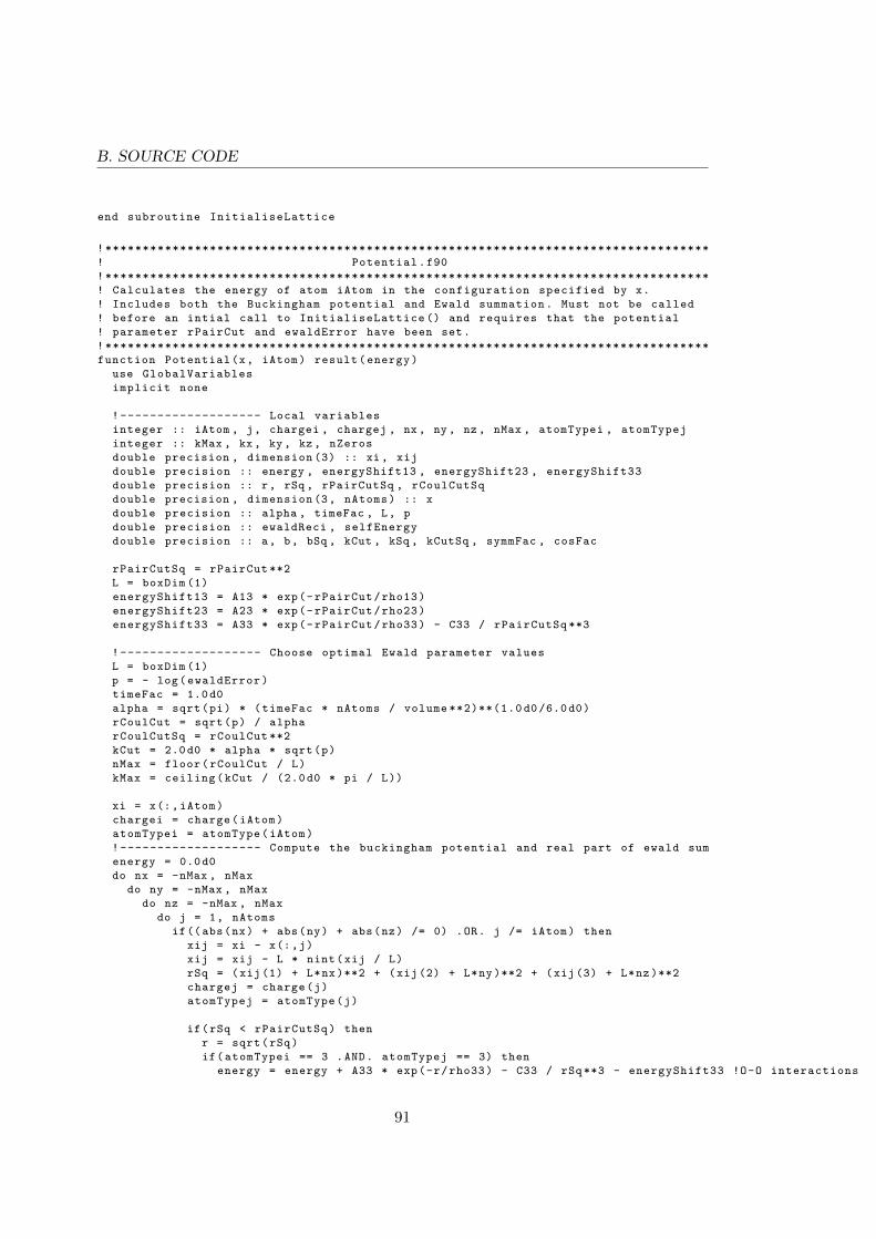
B. SOURCE CODE
end subroutine InitialiseLattice
!*********************************************************************************
! Potential.f90
!*********************************************************************************
! Calculates the energy of atom iAtom in the configuration specified by x.
! Includes both the Buckingham potential and Ewald summation. Must not be called
! before an intial call to InitialiseLattice () and requires that the potential
! parameter rPairCut and ewaldError have been set.
!*********************************************************************************
function Potential(x, iAtom) result(energy)
use GlobalVariables
implicit none
!------------------- Local variables
integer :: iAtom , j, chargei , chargej , nx, ny, nz, nMax , atomTypei , atomTypej
integer :: kMax , kx, ky, kz, nZeros
double precision , dimension (3) :: xi, xij
double precision :: energy , energyShift13 , energyShift23 , energyShift33
double precision :: r, rSq , rPairCutSq , rCoulCutSq
double precision , dimension(3, nAtoms) :: x
double precision :: alpha , timeFac , L, p
double precision :: ewaldReci , selfEnergy
double precision :: a, b, bSq , kCut , kSq , kCutSq , symmFac , cosFac
rPairCutSq = rPairCut **2
L = boxDim (1)
energyShift13 = A13 * exp(-rPairCut/rho13)
energyShift23 = A23 * exp(-rPairCut/rho23)
energyShift33 = A33 * exp(-rPairCut/rho33) - C33 / rPairCutSq **3
!------------------- Choose optimal Ewald parameter values
L = boxDim (1)
p = - log(ewaldError)
timeFac = 1.0d0
alpha = sqrt(pi) * (timeFac * nAtoms / volume **2)**(1.0 d0/6.0d0)
rCoulCut = sqrt(p) / alpha
rCoulCutSq = rCoulCut **2
kCut = 2.0d0 * alpha * sqrt(p)
nMax = floor(rCoulCut / L)
kMax = ceiling(kCut / (2.0d0 * pi / L))
xi = x(:,iAtom)
chargei = charge(iAtom)
atomTypei = atomType(iAtom)
!------------------- Compute the buckingham potential and real part of ewald sum
energy = 0.0d0
do nx = -nMax , nMax
do ny = -nMax , nMax
do nz = -nMax , nMax
do j = 1, nAtoms
if((abs(nx) + abs(ny) + abs(nz) /= 0) .OR. j /= iAtom) then
xij = xi - x(:,j)
xij = xij - L * nint(xij / L)
rSq = (xij(1) + L*nx)**2 + (xij(2) + L*ny)**2 + (xij(3) + L*nz)**2
chargej = charge(j)
atomTypej = atomType(j)
if(rSq < rPairCutSq) then
r = sqrt(rSq)
if(atomTypei == 3 .AND. atomTypej == 3) then
energy = energy + A33 * exp(-r/rho33) - C33 / rSq**3 - energyShift33 !O-O interactions
91

B.3. SOURCE CODE
endif
if(( atomTypei == 1 .AND. atomTypej == 3) &
.OR. (atomTypei == 3 .AND. atomTypej == 1)) then
energy = energy + A13 * exp(-r/rho13) - energyShift13 !Ba-O interactions
endif
if(( atomTypei == 2 .AND. atomTypej == 3) &
.OR. (atomTypei == 3 .AND. atomTypej == 2)) then
energy = energy + A23 * exp(-r/rho23) - energyShift23 !Zr-O interactions
endif
energy = energy + chargei*chargej * erfc(alpha*r) / r
elseif(rSq < rCoulCutSq) then
r = sqrt(rSq)
energy = energy + chargei*chargej * erfc(alpha*r) / r
else
endif
endif
end do
end do
end do
end do
!------------------- Compute the reciprocal part of the ewald sum
ewaldReci = 0.0d0
b = 2.0d0 * pi / L
bSq = b**2
kCutSq = kCut **2
cosFac = 0.0d0
a = 1.0d0 / (4.0d0*alpha **2)
nZeros = 0
symmFac = 0.0d0
do kx = 0, kMax
do ky = 0, kMax
do kz = 0, kMax
kSq = bSq * (kx**2 + ky**2 + kz**2)
if(kSq >= kCutSq .OR. (abs(kx) + abs(ky) + abs(kz)) == 0) then
cycle
endif
nZeros = 0
if(kx == 0) then
nZeros = nZeros + 1
endif
if(ky == 0) then
nZeros = nZeros + 1
endif
if(kz == 0) then
nZeros = nZeros + 1
endif
if(nZeros == 0) then
symmFac = 8.0d0
elseif(nZeros == 1) then
symmFac = 4.0d0
else
symmFac = 2.0d0
endif
do j = 1, nAtoms
xij = x(:,j) - xi
cosFac = cos(b*kx * xij (1)) * cos(b*ky * xij (2)) * cos(b*kz * xij (3))
ewaldReci = ewaldReci + symmFac / kSq * exp(-kSq*a) * chargei*charge(j)* cosFac
end do
end do
end do
end do
92

B. SOURCE CODE
ewaldReci = 4.0d0 * pi * ewaldReci / volume
!------------------- Compute self energy and add together
selfEnergy = -2.0d0 * alpha / sqrt(pi) * chargei **2
energy = energy + selfEnergy + ewaldReci
end function Potential
!*********************************************************************************
! Metropolis.f90
!*********************************************************************************
! Implements the PIMC method with single slice moves and COM displacements.
! Uses auxiliary subroutines InitialisePath () to initialise the path and SquaredDistance
! to compute the minimum image distance squared between two beads. There are also
! subroutines for initialising , updating and writing the averages and histograms
! for the various properties. An initial guess for the parameters controlling then
! ratio of accepted single bead/COM moves is required but are subsequently controlled
! automatically by the program.
!*********************************************************************************
subroutine Metropolis ()
use GlobalVariables
use MersenneTwister
implicit none
!------------------- Local variables
integer :: iRandAtom , iRandSlice , iAtom , iRight , iLeft , iSlice , moveType , iDum , nSpUpdates
integer :: seed , iCycle , ind , nAcceptCOM , nAcceptBead , nTotalCOM , nTotalBead , iHist
integer :: nMovesCOM , nMovesBead , nTotalAcceptCOM , nTotalAcceptBead , nCheck , nCheckCOM
double precision , dimension(3,nAtoms) :: x
double precision , dimension (3) :: xNew , xOld , xRight , xLeft , displaceCOM
double precision , dimension(3, nSlices) :: xSave
double precision :: Potential , potActionOld , potActionNew , kinActionOld , kinActionNew
double precision :: potActionDiff , kinActionDiff , actionDiff , weightRatio , SquaredDistance
double precision :: currentEnergy , lambda , targetRatio , acceptRatioCOM , acceptRatioBead
double precision :: totalEnergy
beta = 1.0d0 / (kBoltz * temperature)
timeStep = beta / nSlices
!------------------- Initialise the Mersenne Twister PRNG
call system_clock(seed)
call init_genrand(seed)
!------------------- Initialise a random path
call InitialisePath ()
!------------------- Main loops
nAcceptBead = 0
nAcceptCOM = 0
nMovesCOM = 0
nMovesBead = 0
nTotalAcceptCOM = 0
nTotalAcceptBead = 0
nTotalBead = 0
nTotalCOM = 0
nCheck = 1
nCheckCOM = 50
targetRatio = 0.50d0
acceptRatioCOM = 0.0d0
acceptRatioBead = 0.0d0
ind = 1
totalEnergy = 0.0d0
93

B.3. SOURCE CODE
call InitialiseProperties ()
do iCycle = 1, nCycles
!----- COM move once per cycle
nTotalCOM = nTotalCOM + 1
nMovesCOM = nMovesCOM + 1
iRandAtom = grndi(nAtoms)
displaceCOM (1) = deltaCOM * (2.0d0 * grnd() - 1.0d0)
displaceCOM (2) = deltaCOM * (2.0d0 * grnd() - 1.0d0)
displaceCOM (3) = deltaCOM * (2.0d0 * grnd() - 1.0d0)
potActionDiff = 0.0d0
do iSlice = 1, nSlices
x = path (:,1:nAtoms ,iSlice)
potActionOld = Potential(x, iRandAtom)
xNew = path(:,iRandAtom ,iSlice) + displaceCOM
xNew = xNew - boxDim * floor(xNew / boxDim)
x(:,iRandAtom) = xNew
xSave(:,iSlice) = xNew
potActionNew = Potential(x,iRandAtom)
potActionDiff = potActionDiff + potActionNew - potActionOld
end do
!----- Metropolis rejection step
actionDiff = timeStep * potActionDiff
if(actionDiff < 0.0d0) then
do iSlice = 1, nSlices
path(:,iRandAtom ,iSlice) = xSave(:,iSlice)
end do
nAcceptCOM = nAcceptCOM + 1
nTotalAcceptCOM = nTotalAcceptCOM + 1
elseif(actionDiff > 75.0d0) then
!if the exponent is too big automatically reject
else
weightRatio = exp(-actionDiff)
if(grnd() <= weightRatio) then
do iSlice = 1, nSlices
path(:,iRandAtom ,iSlice) = xSave(:,iSlice)
end do
nAcceptCOM = nAcceptCOM + 1
nTotalAcceptCOM = nTotalAcceptCOM + 1
else
!reject
endif
endif
do iAtom = 1, nAtoms
!------- Single bead moves
do iDum = 1, nSlices
nTotalBead = nTotalBead + 1
nMovesBead = nMovesBead + 1
iRandSlice = grndi(nSlices)
x = path (:,1:nAtoms ,iRandSlice)
iRandAtom = grndi(nAtoms)
xOld = x(:,iRandAtom)
potActionOld = Potential(x, iRandAtom)
!----- Generate a trial state
xNew (1) = xOld (1) + deltaBead * (2.0d0 * grnd() - 1.0d0)
xNew (2) = xOld (2) + deltaBead * (2.0d0 * grnd() - 1.0d0)
94
B. SOURCE CODE
xNew (3) = xOld (3) + deltaBead * (2.0d0 * grnd() - 1.0d0)
xNew = xNew - boxDim * floor(xNew / boxDim) !translate back into box
x(:,iRandAtom) = xNew
potActionNew = Potential(x, iRandAtom)
potActionDiff = timeStep *( potActionNew - potActionOld)
!----- Ring polymer condition
if(iRandSlice == nSlices) then
iLeft = nSlices - 1
iRight = 1
elseif(iRandSlice == 1) then
iLeft = nSlices
iRight = 2
else
iRight = iRandSlice + 1
iLeft = iRandSlice - 1
endif
xRight = path(:, iRandAtom , iRight)
xLeft = path(:, iRandAtom , iLeft)
!----- Compute the kinetic (spring) energy difference
kinActionOld = SquaredDistance(xOld ,xLeft) + SquaredDistance(xRight ,xOld)
kinActionNew = SquaredDistance(xNew ,xLeft) + SquaredDistance(xRight ,xNew)
kinActionDiff = kinActionNew - kinActionOld
lambda = 0.5d0 / mass(iRandAtom)
kinActionDiff = kinActionDiff / (4 * lambda * timeStep)
actionDiff = potActionDiff + kinActionDiff
!----- Metropolis rejection step
if(actionDiff < 0.0d0) then
!always accept downhill moves
path(:,iRandAtom , iRandSlice) = xNew
nAcceptBead = nAcceptBead + 1
nTotalAcceptBead = nTotalAcceptBead + 1
elseif(actionDiff > 75.0d0) then
!if the exponent is too big automatically reject
else
weightRatio = exp(-actionDiff)
if(grnd() <= weightRatio) then
path(:,iRandAtom , iRandSlice) = xNew
nAcceptBead = nAcceptBead + 1
nTotalAcceptBead = nTotalAcceptBead + 1
else
!reject
endif
endif
end do !------ end do idum
end do !---- end loop over atoms
!------------------- Adjust to get a 50 percent acceptance ratio
if(mod(iCycle , nCheck) == 0) then
acceptRatioBead = dble(nAcceptBead) / dble(nMovesBead)
if(acceptRatioBead < targetRatio) then
deltaBead = deltaBead * 0.98d0
else
deltaBead = deltaBead * 1.02d0
endif
nAcceptBead = 0
nMovesBead = 0
endif
95

B.3. SOURCE CODE
if(mod(iCycle , nCheckCOM) == 0) then
acceptRatioCOM = dble(nAcceptCOM) / dble(nMovesCOM)
if(acceptRatioCOM < targetRatio) then
deltaCOM = deltaCOM * 0.98d0
else
deltaCOM = deltaCOM * 1.02d0
endif
nAcceptCOM = 0
nMovesCOM = 0
endif
!--------- Start updating averages after equilibration
if(iCycle > nBurnIn .AND. pflagSpDensity == 1) then
call TrailMethod ()
endif
if(pflagPairCorr == 1) then
do iSlice = 1, nSlices
call PairCorrelation(path(:,:,iSlice), 1)
nPCorrUpdates = nPCorrUpdates + 1
end do
endif
if(iCycle > nBurnIn .AND. pflagEnergy == 1) then
call EnergyEstimator(currentEnergy)
totalEnergy = totalEnergy + currentEnergy
energyVec(ind) = totalEnergy / dble(iCycle - nBurnIn)
ind = ind + 1
endif
end do !---- end loop over cycles
call AverageProperties ()
call WriteProperties ()
end subroutine Metropolis
!*********************************************************************************
! SquaredDistance.f90
!*********************************************************************************
! Returns the minimum image distance squared between two beads with
! coordinates x1, x2
!*********************************************************************************
function SquaredDistance(x1, x2) result(rSq)
use GlobalVariables
implicit none
double precision :: rSq , xDist , yDist , zDist
double precision , dimension (3) :: x1, x2
xDist = x1(1) - x2(1)
yDist = x1(2) - x2(2)
zDist = x1(3) - x2(3)
xDist = xDist - Lx * nint(xDist / Lx)
yDist = yDist - Ly * nint(yDist / Ly)
zDist = zDist - Lz * nint(zDist / Lz)
rSq = xDist*xDist + yDist*yDist + zDist*zDist
end function SquaredDistance
!*********************************************************************************
! InitialisePath.f90
96
B. SOURCE CODE
!*********************************************************************************
! Initialises a path to be used in the main PIMC simulation
! using the T = 0 equilibrium lattice configuration , requires that
! InitialiseLattice () has already been called.
!*********************************************************************************
subroutine InitialisePath ()
use GlobalVariables
use MersenneTwister
implicit none
!------------------- Local variables
integer :: iSlice , iFirst , iLast , i
double precision , dimension(3, nAtoms) :: x
double precision :: dx
!------------------- Initialise a path
path = 0.0d0
dx = 0.5 * lengthFac
do iSlice = 1,nSlices
x = path (:,1:nAtoms ,iSlice)
do i = 1, nAtoms
x(1,i) = x0(1,i)
x(2,i) = x0(2,i)
x(3,i) = x0(3,i)
end do
path (:,1:nAtoms ,iSlice) = x
end do
path (:,1:nAtoms ,nSlices +1) = 0.0d0
end subroutine InitialisePath
!*********************************************************************************
! EnergyEstimator.f90
!*********************************************************************************
! Implements the direct (Hamiltonian) estimator for the internal energy
!*********************************************************************************
subroutine EnergyEstimator(energy)
use GlobalVariables
implicit none
!------------------- Local variables
double precision :: energy , kinEnergy , potEnergy , constEnergy , lambda , Potential , SquaredDistance
double precision :: kinTmp
integer :: iSlice , iAtom , idm , iRight
double precision , dimension(3,nAtoms) :: x
double precision , dimension (3) :: xRight , xCurr
!------------------- Calculate the total spring energy
kinEnergy = 0.0d0
kinTmp = 0.0d0
do iAtom = 1,nAtoms
kinTmp = 0.0d0
lambda = 0.5d0 / mass(iAtom)
do iSlice = 1, nSlices
iRight = iSlice + 1
if(iRight == nSlices + 1) then
iRight = 1
endif
xRight = path(:,iAtom ,iRight)
xCurr = path(:,iAtom ,iSlice)
kinTmp = kinTmp + SquaredDistance(xCurr , xRight)
97

B.3. SOURCE CODE
end do
kinTmp = kinTmp / lambda
kinEnergy = kinEnergy + kinTmp
end do
kinEnergy = kinEnergy / (4.0d0 * timeStep **2) / dble(nSlices) / dble(nAtoms)
!------------------- Calculate the total potential energy
potEnergy = 0.0d0
do iSlice = 1, nSlices
x = path(:, 1:nAtoms , iSlice)
do iAtom = 1, nAtoms
potEnergy = potEnergy + Potential(x, iAtom)
end do
end do
potEnergy = potEnergy / nSlices
if(nAtoms > 1) then
potEnergy = 0.5d0 * potEnergy
endif
constEnergy = 3.0d0 / timeStep / 2.0d0
energy = constEnergy + potEnergy - kinEnergy
end subroutine EnergyEstimator
!*********************************************************************************
! TrailMethod.f90
!*********************************************************************************
! Computes the single -particle density matrix using the Trail metod
! Adapted to F90 (and slightly modified) from the F77 version found in Brualla (2002).
! The dispFac parameter must be set manually , as an intial
! guess start with a number on the order of the thermal wavelength and then tune
! by hand.
!*********************************************************************************
subroutine TrailMethod ()
use MersenneTwister
use GlobalVariables
implicit none
!------------------- Local variables
integer :: iCut , iSlice , iAtom , typeSelected , iIter , iTmp
integer :: iLeft , iHist , nTypeSelected
double precision :: typeMass , thermalWavel , potActionOld , kinActionOld , Potential
double precision :: kinFac , lambda , mu, dispFac , dx, dy, dz, SquaredDistance
double precision :: kinActionNew , potActionNew , actionDiff , rMax , dr, rMaxSq , r, rSq , L2Sq
double precision , dimension(3, nAtoms) :: x
double precision , dimension(3,nSlices + 1) :: xNew
double precision , dimension (3) :: xLeft , xCurr , xEndDist
double precision :: kinActionDiff , potActionDiff
!------------------- Initialise
typeSelected = 3
if(typeSelected == 3) then
nTypeSelected = nxCells * nyCells * nzCells * 3
elseif(typeSelected < 3) then
nTypeSelected = nxCells * nyCells * nzCells
endif
typeMass = mass(typeSelected)
lambda = 0.5d0 / typeMass
kinFac = 1.0d0 / (4.0d0 * lambda * timeStep)
dispFac = 0.075d0 * lengthFac
rMax = dispFac * 2.0d0
98

B. SOURCE CODE
dr = rMax / nHist
rMaxSq = rMax * rMax
!------------------- Begin main iteration loop
do iIter = 1, nTypeSelected
iCut = grndi(nSlices)
iAtom = grndi(nAtoms)
do while(atomType(iAtom) /= typeSelected)
iAtom = grndi(nAtoms)
end do
xNew = 0.0d0
!------------------- Compute old potential action
potActionOld = 0.0d0
iSlice = iCut
do iTmp = nSlices+1, 1, -1 !note contribution from extra bead
x = path (:,1:nAtoms ,iSlice)
potActionOld = potActionOld + Potential(x, iAtom)
iSlice = iSlice - 1
if(iSlice == 0) then
iSlice = nSlices
endif
end do
potActionOld = timeStep * potActionOld
!------------------- Compute old kinetic action
kinActionOld = 0.0d0
iSlice = iCut
do iTmp = nSlices , 1, -1
iLeft = iSlice - 1
if(iLeft == 0) then
iLeft = nSlices
endif
xLeft = path(:,iAtom ,iLeft)
xCurr = path(:,iAtom ,iSlice)
rSq = SquaredDistance(xLeft ,xCurr)
kinActionOld = kinActionOld + rSq
iSlice = iSlice - 1
if(iSlice == 0) then
iSlice = nSlices
endif
end do
kinActionOld = kinActionOld * kinFac
!------------------- Trail displacement
dx = dispFac * 2.0d0 * (grnd() - 0.5d0)
dy = dispFac * 2.0d0 * (grnd() - 0.5d0)
dz = dispFac * 2.0d0 * (grnd() - 0.5d0)
xNew(:,nSlices + 1) = path(:,iAtom ,iCut) !new bead , doesn ’t move
iSlice = iCut
do iTmp = nSlices , 1, -1
xNew(1,iSlice) = path(1,iAtom ,iSlice) + dx * dble(iTmp) / nSlices
xNew(2,iSlice) = path(2,iAtom ,iSlice) + dy * dble(iTmp) / nSlices
xNew(3,iSlice) = path(3,iAtom ,iSlice) + dz * dble(iTmp) / nSlices
xNew(:,iSlice) = xNew(:,iSlice) - boxDim * floor(xNew(:,iSlice) / boxDim)
iSlice = iSlice - 1
if(iSlice == 0) then
iSlice = nSlices
endif
end do
!------------------- Compute new kinetic action
99

B.3. SOURCE CODE
iSlice = iCut
kinActionNew = 0.0d0
do iTmp = nSlices , 1, -1
iLeft = iSlice - 1
if(iLeft == 0) then
iLeft = nSlices
endif
if(iTmp == 1) then
iLeft = nSlices + 1
endif
xLeft = xNew(:,iLeft)
xCurr = xNew(:,iSlice)
rSq = SquaredDistance(xLeft ,xCurr)
kinActionNew = kinActionNew + rSq
iSlice = iSlice - 1
if(iSlice == 0) then
iSlice = nSlices
endif
end do
kinActionNew = kinActionNew * kinFac
!------------------- Compute new potential action & action difference
potActionNew = 0.0d0
iSlice = iCut
do iTmp = nSlices , 1, -1
x = path (:,1:nAtoms ,iSlice)
x(:,iAtom) = xNew(:,iSlice)
potActionNew = potActionNew + Potential(x, iAtom)
iSlice = iSlice - 1
if(iSlice == 0) then
iSlice = nSlices
endif
end do
x = path (:,1:nAtoms ,iCut)!contribution from extra bead
x(:,iAtom) = xNew(:,nSlices + 1)
potActionNew = potActionNew + Potential(x, iAtom)
potActionNew = timeStep * potActionNew
actionDiff = potActionNew + kinActionNew - &
potActionOld - kinActionOld
!------------------- Compute end -to-end distance & add to histogram
xEndDist = path(:,iAtom ,iCut) - xNew(:,iCut)
xEndDist = xEndDist - boxDim * nint(xEndDist / boxDim)
rSq = xEndDist (1)**2 + xEndDist (2)**2 + xEndDist (3)**2
if(rSq <= rMaxSq) then
r = sqrt(rSq)
iHist = int(r / dr) + 1
if(iHist < nHist) then
actionDiff = exp(-actionDiff)
if(actionDiff > tmpMax) then
tmpMax = actionDiff
endif
endHist(iHist) = endHist(iHist) + 1
actionHist(iHist) = actionHist(iHist) + actionDiff
endif
endif
end do !end main iteration loop
end subroutine TrailMethod
!*********************************************************************************
100
B. SOURCE CODE
! MetropolisBisection.f90
!*********************************************************************************
! Same as the Metropolis.f90 program but with bisection moves instead of single
! slice moves.
!*********************************************************************************
subroutine MetropolisBisection ()
use GlobalVariables
use MersenneTwister
implicit none
!------------------- Local variables
integer , parameter :: intKind = selected_int_kind (11)
integer(kind = intKind) :: nTotalAcceptCOM , nTotalCOM , nAcceptBisect , nTotalBisect
integer :: iRandAtom , iRandSlice , iAtom , iLeft , iSlice , moveType , iDum , nSpUpdates
integer :: seed , iCycle , ind , nAcceptCOM , iHist
integer :: nMovesCOM , nCheck
double precision , dimension(3,nAtoms) :: x
double precision , dimension (3) :: xNew , xOld , xLeft , displaceCOM
double precision , dimension(3, nSlices) :: xSave
double precision :: Potential , potActionOld , potActionNew , kinActionOld , kinActionNew
double precision :: potActionDiff , kinActionDiff , actionDiff , weightRatio , SquaredDistance
double precision :: currentEnergy , lambda , targetRatio , acceptRatioCOM , acceptRatioBead , totalEnergy
integer , parameter :: nLevels = 2
integer , parameter :: nClip = 2** nLevels + 1
integer :: iLevel , iClipFirst , iTmp , iBead , iStep , iFirst , iLast , iLow , iHigh , iRight , iClip
integer :: flagProceed , nCurrLevel , nMoved
double precision , dimension(3, nClip) :: xClip , xClipSave
double precision , dimension (3) :: xLow , xBead , xHigh , xRight , xCurr
double precision :: rnorm , variance , timeDiff , kinFac , potActionDiffPrev
beta = 1.0d0 / (kBoltz * temperature)
timeStep = beta / nSlices
!------------------- Initialise the Mersenne Twister PRNG
call system_clock(seed)
call init_genrand(seed)
!------------------- Initialise a random path
call InitialisePath ()
!------------------- Main loops
nAcceptCOM = 0
nMovesCOM = 0
nTotalAcceptCOM = 0
nTotalCOM = 0
nCheck = 100
targetRatio = 0.50d0
acceptRatioCOM = 0.0d0
nAcceptBisect = 0
nTotalBisect = 0
ind = 1
totalEnergy = 0.0d0
nPCorrUpdates = 0
call InitialiseProperties ()
do iCycle = 1, nCycles
!--------------------------
!Do COM moves
!--------------------------
101

B.3. SOURCE CODE
if(nSlices /= 1) then
!----------- Bisection moves
do iAtom = 1, nAtoms
nTotalBisect = nTotalBisect + 1
!iRandAtom = grndi(nAtoms) !polymer to bisect
iRandAtom = iAtom
lambda = 0.5d0 / mass(iRandAtom)
iClipFirst = grndi(nSlices) !starting bead of the clip
iSlice = iClipFirst
do iClip = 1, nClip !map the clip from path to xClip
xClip(:,iClip) = path(:, iRandAtom , iSlice)
xClipSave(:,iClip) = xClip(:,iClip)
iSlice = iSlice + 1
if(iSlice == nSlices + 1) then
iSlice = 1
endif
end do
!------ Loop over levels , starting at the coarsest level
potActionDiffPrev = 0.0d0
flagProceed = 0
do iLevel = nLevels , 1, -1
iStep = 2**( iLevel -1)
timeDiff = timeStep * dble(iStep)
variance = sqrt(lambda * timeDiff)
nMoved = 2**( nLevels - iLevel) !#beads sampled in current level
!--- Sample new beads in current level
iClip = 1 + iStep !index of first bead to be sampled in current level
do iTmp = 1, nMoved
iLow = iClip - iStep
iHigh = iClip + iStep
xCurr = xClip(:,iClip)
xLow = xCurr - xClip(:,iLow) !sample new bead
xHigh = xClip(:,iHigh) - xCurr
xLow = xLow - Lx * nint(xLow / Lx)
xHigh = xHigh - Lx * nint(xHigh / Lx)
xLow = xCurr - xLow
xHigh = xCurr + xHigh
xClip(1,iClip) = 0.5d0 * (xLow (1) + xHigh (1)) + variance * rnorm()
xClip(2,iClip) = 0.5d0 * (xLow (2) + xHigh (2)) + variance * rnorm()
xClip(3,iClip) = 0.5d0 * (xLow (3) + xHigh (3)) + variance * rnorm()
xClip(:,iClip) = xClip(:,iClip) - Lx * floor(xClip(:,iClip) / Lx)
iClip = iClip + 2 * iStep !proceed to next bead in current level
end do
!--- Calculate potential action difference
nCurrLevel = 2**( nLevels - iLevel + 1) - 1 !beads in current level
potActionOld = 0.0d0
potActionNew = 0.0d0
iClip = 1 + iStep
iSlice = iClipFirst + iStep
if(iSlice > nSlices) then
iSlice = iSlice - nSlices
endif
do iTmp = 1, nCurrLevel
x = path (:,1:nAtoms ,iSlice)
potActionOld = potActionOld + Potential(x, iRandAtom)
x(:,iRandAtom) = xClip(:,iClip)
potActionNew = potActionNew + Potential(x, iRandAtom)
iClip = iClip + iStep
102
B. SOURCE CODE
iSlice = iSlice + iStep
if(iSlice > nSlices) then
iSlice = iSlice - nSlices
endif
end do
potActionDiff = timeDiff * (potActionNew - potActionOld)
!--- Metropolis rejection step
actionDiff = potActionDiff - potActionDiffPrev
potActionDiffPrev = potActionDiff
if(actionDiff < 0.0d0) then
flagProceed = 1 !proceed to next level
elseif(actionDiff > 75.0d0) then
flagProceed = 0 !reject entire move
exit
else
weightRatio = exp(-actionDiff)
if(grnd() <= weightRatio) then
flagProceed = 1 !proceed to next level
else
flagProceed = 0
exit
endif
endif
end do !---- end loop over levels
if(flagProceed == 1) then !bisection move was accepted
nAcceptBisect = nAcceptBisect + 1
iSlice = iClipFirst
do iClip = 1, nClip
path(:,iRandAtom ,iSlice) = xClip(:,iClip)
iSlice = iSlice + 1
if(iSlice == nSlices + 1) then
iSlice = 1
endif
enddo
else !else revert to old positions
iSlice = iClipFirst
do iClip = 1, nClip
path(:,iRandAtom ,iSlice) = xClipSave(:,iClip)
iSlice = iSlice + 1
if(iSlice == nSlices + 1) then
iSlice = 1
endif
enddo
endif
end do !---- end loop over atoms
endif !--- end if nSlices /= 1
!--------------------------------------------
!Adjust to get a 50 percent acceptance ratio for COM moves
!---------------------------------------
!--------------------------------------------
! Calculate and update properties
!---------------------------------------
103

B.3. SOURCE CODE
end do !---- end loop over cycles
call AverageProperties ()
call WriteProperties ()
end subroutine MetropolisBisection
!*********************************************************************************
! OpenChain.f90
!*********************************************************************************
! The open chain algortihm for calculating the end -to-end distance distribution.
! Note that this basically includes the entire PIMC main code since using an
! open chain requires a specific simulaton and no other diagonal properties
! can be calculated at the same time.
!*********************************************************************************
subroutine MetropolisOpen ()
use GlobalVariables
use MersenneTwister
implicit none
!------------------- Local variables
integer :: iRandAtom , iRandSlice , iAtom , iRight , iLeft , iSlice
integer :: moveType , iDum , nSpUpdates , nLast , iOpenAtom
integer :: nPCorrUpdates , seed , iCycle , ind , nAcceptCOM
integer :: nAcceptBead , nTotalCOM , nTotalBead , iHist , iCut
integer :: flagCase , iCutNext
double precision , dimension(3,nAtoms) :: x
double precision , dimension (3) :: xNew , xOld , xRight , xLeft , displaceCOM , xEndDist
double precision , dimension(3, nSlices +1) :: xSave
double precision :: Potential , potActionOld , potActionNew , kinActionOld , kinActionNew
double precision :: potActionDiff , kinActionDiff , actionDiff , weightRatio
double precision :: currentEnergy , lambda , r, rMax , rSq , rMaxSq , dr, SquaredDistance
beta = 1.0d0 / (kBoltz * temperature)
timeStep = beta / nSlices
!------------------- Initialise the Mersenne Twister PRNG
call system_clock(seed)
call init_genrand(seed)
!------------------- Initialise a random path
call InitialisePath ()
!------------------- Main loops
nAcceptBead = 0
nAcceptCOM = 0
nTotalBead = 0
nTotalCOM = 0
flagCase = 0
!open chain
iOpenAtom = 34
iCut = grndi(nSlices)
iCutNext = iCut + 1
if(iCutNext == nSlices + 1) then
iCutNext = 1
endif
path(:,iOpenAtom ,nSlices + 1) = path(:,iOpenAtom ,iCut)
!rMax = boxDim (1) / 2.0d0 !for the histogram
rMax = 0.6d0 * lengthFac
dr = rMax / dble(nHist)
104

B. SOURCE CODE
rMaxSq = rMax * rMax
do iCycle = 1, nCycles
!------------------- Centre of mass displacement
nTotalCOM = nTotalCOM + 1
iRandAtom = grndi(nAtoms)
displaceCOM (1) = deltaCOM * (2.0d0 * grnd() - 1.0d0)
displaceCOM (2) = deltaCOM * (2.0d0 * grnd() - 1.0d0)
displaceCOM (3) = deltaCOM * (2.0d0 * grnd() - 1.0d0)
if(iRandAtom == iOpenAtom) then
nLast = nSlices + 1
else
nLast = nSlices
endif
potActionDiff = 0.0d0
do iSlice = 1, nLast
x = path(:,:,iSlice)
potActionOld = Potential(x, iRandAtom)
xNew = path(:,iRandAtom ,iSlice) + displaceCOM
xNew = xNew - boxDim * floor(xNew / boxDim)
x(:,iRandAtom) = xNew
xSave(:,iSlice) = xNew
potActionNew = Potential(x,iRandAtom)
potActionDiff = potActionDiff + potActionNew - potActionOld
end do
!----- Metropolis rejection step
actionDiff = timeStep * potActionDiff
if(actionDiff < 0.0d0) then
do iSlice = 1, nLast
path(:,iRandAtom ,iSlice) = xSave(:,iSlice)
end do
nAcceptCOM = nAcceptCOM + 1
elseif(actionDiff > 75.0d0) then
!if the exponent is too big automatically reject
else
weightRatio = exp(-actionDiff)
if(grnd() <= weightRatio) then
do iSlice = 1, nLast
path(:,iRandAtom ,iSlice) = xSave(:,iSlice)
end do
nAcceptCOM = nAcceptCOM + 1
else
!reject
endif
endif
do iAtom = 1, nAtoms
!------------------- Single bead moves
do iDum = 1, nSlices
nTotalBead = nTotalBead + 1
iRandAtom = grndi(nAtoms)
if(iRandAtom == iOpenAtom) then
nLast = nSlices + 1
else
nLast = nSlices
endif
iRandSlice = grndi(nLast)
x = path(:,:, iRandSlice)
105
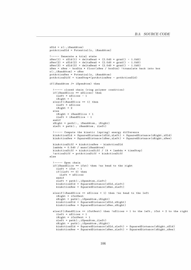
B.3. SOURCE CODE
xOld = x(:,iRandAtom)
potActionOld = Potential(x, iRandAtom)
!----- Generate a trial state
xNew (1) = xOld (1) + deltaBead * (2.0d0 * grnd() - 1.0d0)
xNew (2) = xOld (2) + deltaBead * (2.0d0 * grnd() - 1.0d0)
xNew (3) = xOld (3) + deltaBead * (2.0d0 * grnd() - 1.0d0)
xNew = xNew - boxDim * floor(xNew / boxDim) !translate back into box
x(:,iRandAtom) = xNew
potActionNew = Potential(x, iRandAtom)
potActionDiff = timeStep *( potActionNew - potActionOld)
if(iRandAtom /= iOpenAtom) then
!----- closed chain (ring polymer condition)
if(iRandSlice == nSlices) then
iLeft = nSlices - 1
iRight = 1
elseif(iRandSlice == 1) then
iLeft = nSlices
iRight = 2
else
iRight = iRandSlice + 1
iLeft = iRandSlice - 1
endif
xRight = path(:, iRandAtom , iRight)
xLeft = path(:, iRandAtom , iLeft)
!----- Compute the kinetic (spring) energy difference
kinActionOld = SquaredDistance(xOld ,xLeft) + SquaredDistance(xRight ,xOld)
kinActionNew = SquaredDistance(xNew ,xLeft) + SquaredDistance(xRight ,xNew)
kinActionDiff = kinActionNew - kinActionOld
lambda = 0.5d0 / mass(iRandAtom)
kinActionDiff = kinActionDiff / (4 * lambda * timeStep)
!actionDiff = potActionDiff + kinActionDiff
else
!----- Open chain
if(iRandSlice == iCut) then !no bead to the right
iLeft = iCut - 1
if(iLeft == 0) then
iLeft = nSlices
endif
xLeft = path(:,iOpenAtom ,iLeft)
kinActionOld = SquaredDistance(xOld ,xLeft)
kinActionNew = SquaredDistance(xNew ,xLeft)
elseif(iRandSlice == nSlices + 1) then !no bead to the left
iRight = iCutNext
xRight = path(:,iOpenAtom ,iRight)
kinActionOld = SquaredDistance(xOld ,xRight)
kinActionNew = SquaredDistance(xNew ,xRight)
elseif(iRandSlice == iCutNext) then !nSlices + 1 to the left , iCut + 2 to the right
iLeft = nSlices + 1
iRight = iCutNext + 1
xLeft = path(:,iOpenAtom ,iLeft)
xRight = path(:,iOpenAtom ,iRight)
kinActionOld = SquaredDistance(xOld ,xLeft) + SquaredDistance(xRight ,xOld)
kinActionNew = SquaredDistance(xNew ,xLeft) + SquaredDistance(xRight ,xNew)
106

B. SOURCE CODE
else !beads in both directions
iRight = iRandSlice + 1
iLeft = iRandSlice - 1
if(iRight == nSlices + 1) then
iRight = 1
endif
if(iLeft == 0) then
iLeft = nSlices
endif
xLeft = path(:,iOpenAtom ,iLeft)
xRight = path(:,iOpenAtom ,iRight)
kinActionOld = SquaredDistance(xOld ,xLeft) + SquaredDistance(xRight ,xOld)
kinActionNew = SquaredDistance(xNew ,xLeft) + SquaredDistance(xRight ,xNew)
endif
lambda = 0.5d0 / mass(iRandAtom)
kinActionDiff = kinActionNew - kinActionOld
kinActionDiff = kinActionDiff / (4 * lambda * timeStep)
endif !----- End open / closed chain
actionDiff = potActionDiff + kinActionDiff
!----- Metropolis rejection step (regardless of open/closed chain)
if(actionDiff < 0.0d0) then
!always accept downhill moves
path(:,iRandAtom , iRandSlice) = xNew
nAcceptBead = nAcceptBead + 1
elseif(actionDiff > 75.0d0) then
!if the exponent is too big automatically reject
else
weightRatio = exp(-actionDiff)
if(grnd() <= weightRatio) then
path(:,iRandAtom , iRandSlice) = xNew
nAcceptBead = nAcceptBead + 1
else
!reject
endif
endif
end do !---- end do idum
end do !---- end loop over atoms
if(iCycle > nBurnIn) then
!end to end distance histogram
xEndDist = path(:,iOpenAtom ,iCut) - path(:,iOpenAtom ,nSlices + 1)
xEndDist = xEndDist - boxDim * nint(xEndDist / boxDim)
rSq = xEndDist (1)**2 + xEndDist (2)**2 + xEndDist (3)**2
if(rSq <= rMaxSq) then
r = sqrt(rSq)
iHist = int(r / dr) + 1
if(iHist < nHist) then
endHist(iHist) = endHist(iHist) + 1
endif
endif
endif
end do !---- end loop over cycles
end subroutine MetropolisOpen
107
