The More you Learn, the Less you Store:

Memory-controlled Incremental SVM for

Visual Place Recognition

Andrzej Pronobis a,∗, Luo Jie b,c, Barbara Caputo b,

aCAS/CVAP, The Royal Institute of Technology (KTH), Stockholm, SwedenbIdiap Research Institute, Martigny, Switzerland

cSwiss Federal Institute of Technology in Lausanne (EPFL), Switzerland

Abstract

The capability to learn from experience is a key property for autonomous cognitivesystems working in realistic settings. To this end, this paper presents an SVM--based algorithm, capable of learning model representations incrementally whilekeeping under control memory requirements. We combine an incremental extensionof SVMs [45] with a method reducing the number of support vectors needed to buildthe decision function without any loss in performance [15] introducing a parameterwhich permits a user-set trade-off between performance and memory. The resultingalgorithm is able to achieve the same recognition results as the original incrementalmethod while reducing the memory growth. Our method is especially suited towork for autonomous systems in realistic settings. We present experiments on twocommon scenarios in this domain: adaptation in presence of dynamic changes andtransfer of knowledge between two different autonomous agents, focusing in bothcases on the problem of visual place recognition applied to mobile robot topologicallocalization. Experiments in both scenarios clearly show the power of our approach.

Key words: incremental learning, knowledge transfer, support vector machines,place recognition, visual robot localization

∗ Corresponding author.Email addresses: pronobis@csc.kth.se (Andrzej Pronobis), jluo@idiap.ch

(Luo Jie), bcaputo@idiap.ch (Barbara Caputo).

Preprint submitted to Elsevier 26 January 2010

1 Introduction

Many recent advances in fields such as computer vision and robotics havebeen driven by the ultimate goal of creating artificial cognitive systems ableto perform human-like tasks. Several attempts have been made to create in-tegrated cognitive architectures and implement them, for instance, on mobilerobots [2,23,1,3]. The ability to learn and interpret complex sensory informa-tion based on the previous experience, inherently connected with cognition,has been recognized as crucial and vastly researched [43,41,34]. In most cases,the recognition systems used are trained offline, i.e. they are based on batchlearning algorithms. However, in the real, dynamic world, learning cannot bea single act. It is simply not possible to create a static model which couldexplain all the variability observed over time. Continuous information acqui-sition and exchange, coupled with an ongoing learning process, is necessary toprovide a cognitive system with a valid world representation.

In artificial autonomous agents constrained by limited resources (such as mo-bile robots), continuous learning must be performed in an incremental fashion.It is obviously not feasible to rebuild the internal model from scratch everytime new information arrives, neither it is possible to store all the previouslyacquired data for that purpose. The model must be updated and the updatingprocess must have certain properties. First, the knowledge representation mustremain compact and free from redundancy to fit into the limited memory andmaintain a fixed computational complexity. We call this property controlledmemory growth. Second, in the continuous learning scenario, a model cannotgrow forever even though new information is constantly arriving. Thus, the up-dating process should be able to gradually filter out unnecessary information.We call this property forgetting capability.

Discriminative methods have become widely popular for visual recognition,achieving impressive results on several applications [49,20,14]. Within discrim-inative classifiers, SVM techniques provide powerful tools for learning modelswith good generalization capabilities; in some domains like object and materialcategorization, SVM-based algorithms are state of the art [7,17]. This makesit worth it to investigate whether it is possible to perform continuous learn-ing with this type of methods. Several incremental extensions of SVMs havebeen proposed in the machine learning community [13,8,45,36]. Between thesemethods, the approximate techniques [13,45] seem better suited for visualrecognition because, at each incremental step, they discard non-informativetraining vectors, thus reducing the memory requirements. Other methods,such as [8,36], instead require to store in memory all the training data, even-tually leading to a memory explosion; this makes them unfit for real-timeautonomous systems.

2

This paper presents an SVM-based incremental method which performs likethe batch algorithm while reducing the memory requirements. We combine anapproximate technique for incremental SVM [45] with an exact method thatreduces the number of support vectors needed to build the decision functionwithout any loss in performance [15]. This results in an algorithm performingas the original incremental method with a reduction in the memory require-ments. We then present an extension of the method for the exact simplificationof the support vector solution [15]. We introduce a parameter that links theperformance of an SVM to the amount of vectors that is possible to discard.This allows a user-set trade-off between performance and memory reduction.

We evaluate the suitability of our method for autonomous cognitive systemsin two challenging scenarios: adaptation in presence of dynamic changes andtransfer of knowledge between autonomous agents. In both cases, we con-centrate on the problem of visual place recognition applied to mobile robottopological localization. The problem is important from the point of view ofengineering cognitive systems, as it allows to tie semantics with space repre-sentations and provides solutions for typical problems with purely metric lo-calization. However, it is also a challenging recognition problem as it requiresprocessing of large amounts of high-dimensional visual information which isnoisy and dynamic in nature. In this context, the memory and computationalefficiency become one of the most important properties of the learning algo-rithm determining the design choice.

In our considerations, we first focus on the scenario in which the incrementallearning is used to provide adaptability to different types of variations observedin real-world environments. In our previous work [40,38], we presented a purelyappearance-based model able to cope with illumination and pose changes,and we showed experimentally that it could achieve satisfactory performanceswhen considering short time intervals between the acquisition of the trainingand testing data. Nevertheless, a room’s appearance is doomed to changedramatically over time because it is used: chairs are pushed around, objectsare taken in/out of drawers, furniture and paintings are added, or changed, orre-arranged; and so forth. As it is not possible to predict a priori how a roomis going to change, the only possible strategy is to update the representationover time, learning incrementally from the new data recorded during use.

As a second scenario, we consider the case when a robot, proficient in solvingthe place recognition task within a known environment, transfers its visualknowledge to another robotic platform with different characteristics, which isa tabula rasa. The ability to transfer knowledge between different domainsenables humans to learn efficiently from small number of examples. This ob-servation inspired robotics and machine learning researchers to search for algo-rithms able to exploit prior knowledge so to improve performance of artificiallearners and speed up the learning process. To tackle this problem, it is neces-

3

sary an efficient way of exploiting the knowledge transferred from a differentplatform as well as updating the internal representation when new trainingdata are available. The knowledge transfer scheme should be adaptive andprivilege newest data so to prevent from accumulating outdated information.Finally, the solution obtained starting from a transferred model should gradu-ally converge to the one learned from scratch, not only in terms of performanceon a task but also of required resources (e.g. memory).

To achieve these goals, we used our memory-controlled incremental SVM andwe evaluated its performance in terms of accuracy, memory growth, complex-ity and forgetting capability. We compare the results obtained by our methodwith those achieved by the batch algorithm and by two other incrementalextensions of SVMs, one approximate (the fixed-partition incremental SVM,[45]) and one exact (online independent SVM, [36]). We evaluated the algo-rithms on a visual place recognition database acquired using two mobile robotplatforms [40], which we extended with new data acquired 6 months later us-ing the same hardware. Then, we confirmed the results on another databaseacquired in a different environment and using different hardware [39]. To testthe adaptability of the recognition system, we performed topological localiza-tion experiments under realistic long-term variations. To test the knowledgetransfer capabilities, we performed experiments in case of which visual knowl-edge captured in the SVM model was gradually exchanged between the twomobile robot platforms. The experiments clearly show the power of our ap-proach in both scenarios, while illustrating the need for incremental solutionsin artificial cognitive systems.

The rest of the paper is organized as follows: after a review of related work(Section 2), Section 3 gives our working definition of visual place recognitionfor robot localization. Section 4 reviews SVMs, it introduces the memory-controlled incremental SVM algorithm, which will constitute a building blockof the adaptive place recognition system and a base for our knowledge transfertechnique, and it briefly describes two other incremental extensions of SVMsagainst which we will benchmark our approach. Section 5 describes our exper-imental setup; Section 7 concentrates on the adaptation problem and presentsexperimental evaluation of the algorithms in this context. Finally, Section 8gives details of our approach to the transfer of knowledge and shows its effec-tiveness with a set of experiments. The paper concludes with a summary andpossible directions for future work.

2 Related Work

In the last years, the need for solutions to such problems as robustness tolong-term dynamic variations or transfer of knowledge is more and more ac-

4

knowledged. In [41], the authors tried to deal with long-term visual variationsin indoor environments by combining information acquired using two sensors ofdifferent characteristics. In [51], the problem of invariance to seasonal changesin appearance of an outdoor environment is addressed. Clearly, adaptabilityis a desirable property of a recognition system. At the same time, Thrun andMitchell [48,33] studied the issue of exchanging knowledge related to differenttasks in the context of artificial neural networks and argued for the importanceof knowledge-transfer schemes for lifelong robot learning. Several attempts tosolve the problem have also been made from the perspective of ReinforcementLearning, including the case of transferring learned skills between different RLagents [30,21].

The work conducted in the fields of cognitive robotics and vision stimulatedthe research in the machine learning community directed towards develop-ing extensions for algorithms that were commonly used due to their superiorperformance but were missing the ability to be trained incrementally. As aresult, methods such as Incremental PCA have been invented and successfullyapplied e.g. for mobile robot localization [4,11]. As it was already mentioned,several incremental extensions have been introduced also for Support VectorMachines [13,8,45]. Between these methods, the approximate techniques[13,45]seem better suited for visual recognition because, at each incremental step,they discard non-informative training vectors, thus reducing the memory re-quirements. Other methods, such as [8,36], or simple KNN-based solutions,instead require to store in memory all the training data, eventually leadingto a memory explosion. This limits their usefulness for complex real-worldproblems involving continuous learning of visual patterns.

Despite the fact that the approximate incremental SVM extensions allow toreduce the amount of data stored during the learning process, there is no guar-antee that the continuously updated model will not grow forever. Additionally,the results of experiments that can be found in the literature do not give aclear answer if it is possible to apply such methods for complex problems suchas visual place recognition or transfer of visual knowledge.

3 Visual Place Recognition for Robot Localization

In this section, we give our working definition of visual place recognition, ex-plaining how it can be applied to mobile robot topological localization. Wedefine a place as a nameable segment of a real-world environment, uniquelyidentifiable because of its specific functionality and/or appearance. Examplesof places, according to this definition, are a kitchen, an office, a corridor, andso forth. We adopt the appearance-based paradigm, and we assume that a re-alistic scene can be represented by a visual descriptor without any loss of dis-

5

∃&.&#∃Χ

Training

Testing

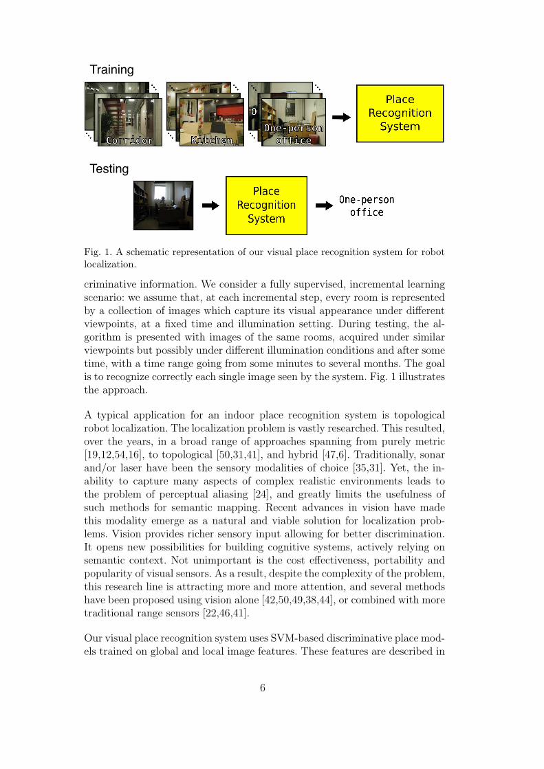
Fig. 1. A schematic representation of our visual place recognition system for robotlocalization.

criminative information. We consider a fully supervised, incremental learningscenario: we assume that, at each incremental step, every room is representedby a collection of images which capture its visual appearance under differentviewpoints, at a fixed time and illumination setting. During testing, the al-gorithm is presented with images of the same rooms, acquired under similarviewpoints but possibly under different illumination conditions and after sometime, with a time range going from some minutes to several months. The goalis to recognize correctly each single image seen by the system. Fig. 1 illustratesthe approach.

A typical application for an indoor place recognition system is topologicalrobot localization. The localization problem is vastly researched. This resulted,over the years, in a broad range of approaches spanning from purely metric[19,12,54,16], to topological [50,31,41], and hybrid [47,6]. Traditionally, sonarand/or laser have been the sensory modalities of choice [35,31]. Yet, the in-ability to capture many aspects of complex realistic environments leads tothe problem of perceptual aliasing [24], and greatly limits the usefulness ofsuch methods for semantic mapping. Recent advances in vision have madethis modality emerge as a natural and viable solution for localization prob-lems. Vision provides richer sensory input allowing for better discrimination.It opens new possibilities for building cognitive systems, actively relying onsemantic context. Not unimportant is the cost effectiveness, portability andpopularity of visual sensors. As a result, despite the complexity of the problem,this research line is attracting more and more attention, and several methodshave been proposed using vision alone [42,50,49,38,44], or combined with moretraditional range sensors [22,46,41].

Our visual place recognition system uses SVM-based discriminative place mod-els trained on global and local image features. These features are described in

6

details in Section 5. The classification algorithm is introduced in Section 4. Inour experiments, we always used only a single image as input for the recog-nition system. This makes the recognition problem harder, but also it makesit possible to perform global localization where no prior knowledge about theposition is available (e.g. in case of the kidnapped robot problem). Spatial ortemporal filtering can be used together with the presented method to enhanceperformance.

4 Memory-controlled Incremental SVM

This section describes our algorithmic approach to incremental learning ofvisual place models. We propose a fully supervised, SVM-based method withcontrolled memory growth that tends to privilege newest information overolder data. This leads to a system able to adapt over time to the naturalchanges of a real-world setting, while maintaining a limited memory size andcomputational complexity.

The rest of this section describes the basic principles of Support Vector Ma-chines (Section 4.1), a popular incremental extension of the basic algorithm(Section 4.2), our memory-controlled version of incremental SVM (Section 4.3)and an exact method based on a similar intuition (Section 4.4), with whichwe will compare our approach.

4.1 SVM: the batch algorithm

Consider the problem of separating the set of training data (x1, y1), . . . (xm, ym)into two classes, where xi ∈ ℜN is a feature vector and yi ∈ {−1, +1} its classlabel (for multi-class extensions, we refer the reader to [10,52]). If we assumethat the two classes can be linearly separated when mapped to some higherdimensional Hilbert space H by x → Φ(x) ∈ H (see [10,52] for solutions tonon-separable cases), the optimal hyperplane is the one which has maximumdistance to the closest points in the training set, resulting in a classificationfunction:

f(x) = sgn

(m∑

i=1

αiyiK(xi, x) + b

), (1)

where K(x, y) = Φ(x) ·Φ(y) is the kernel function. Most of the αi’s take thevalue of zero; xi with nonzero αi are the Support Vectors (SV). Different ker-nel functions correspond to different similarity measures. Choosing a suitablekernel can therefore have a strong impact on the performance of the classifier.Based on results reported in the literature [40], here we used the two followingkernels:

7

• The χ2 kernel [5] for histogram-like global descriptors:

K(x, y) = exp{−γχ2(x, y)}, χ2(x, y) =N∑

i=1

(xi − yi)2

xi + yi

;

• The matching kernel [53] for local features:

K(Lh, Lk) =1

nh

nh∑

jh=1

maxjk=1,...,nk

{Kl(L

jh

h , Ljk

k )}

,

where Lh, Lk are local feature sets and Ljh

h , Ljk

k are two single local features.The sum is always calculated over the smaller set of local features and onlysome fixed amount of best matches is considered in order to exclude outliers.The local feature similarity kernel Kl can be any Mercer kernel. We usedthe RBF kernel based on the Euclidean distance for the SIFT [27] features:

Kl(Ljh

h , Ljk

k ) = exp{−γ||Ljh

h − Ljk

k ||2}

.

4.2 SVM: an Incremental Extension

Among the incremental SVM extensions proposed so far [45,13,8], approximatemethods seem to be the most suitable for visual recognition, because theydiscard a significant amount of the training data at each incremental step.Exact methods instead need to retain all training samples in order to preservethe convexity of the solution at each incremental step. As a consequence,they require huge amounts of memory when employed in realistic, continuouslearning scenario as the one we consider here. Approximate methods avoidthis problem by sacrificing the guaranteed optimality of the solution. Still,several studies showed that they generally achieve performances very similarto those obtained by an SVM trained on the complete data set (see [13] andreferences therein), because at each incremental step the algorithm remembersthe essential class boundary information regarding the data seen so far (inform of support vectors). This information contributes properly to generatethe classifier at the next iteration.

Once a new batch of data is loaded into memory, there are different possibilitiesfor performing the update of the current model, which might discard a part ofthe new data according to some fixed criteria [13,45]. For all the techniques,at each step only the learned model from the data previously seen (preservedin form of SV) is kept in memory. In this paper we will consider the fixed-partition method [45]. Here the training data set is partitioned in batches ofsome size k:

T = {T 1, T 2, . . . T n},

8

Fig. 2. The fixed-partition incremental SVM algorithm.

with T i = {(xij, y

ij)}

kj=1. At the first step, the model is trained on the first

batch of data T 1, obtaining a classification function

f1(x) = sgn

(m1∑

i=1

α1

i y1

i K(x1

i , x) + b1

). (2)

At the second step, a new batch of data is loaded into memory and added tothe current set of support vectors; then, the new training set becomes

T inc2 = {T 2 ∪ SV 1}, SV 1 = {(x1

i , y1

i )}m1

i=1,

where SV 1 are the support vectors learned at the first step. The new classi-fication function will be:

f2(x) = sgn

(m2∑

i=1

α2

i y2

i K(x2

i , x) + b2

).

Thus, as new batches of data points are loaded into memory, the existingsupport vector model is updated, so to generate the classifier at that incre-mental step. The method is illustrated in Fig. 2. Note that this incrementalmethod can be seen as an approximation of the chunking technique used fortraining SVM [10,52]. Indeed, the chunking algorithm is an exact decompo-sition which iterates through the training set to select the support vectors.The fixed-partition incremental method instead scan through the trainingdata just once, and once discarded, does not consider them anymore. Thefixed-partition incremental algorithm has been tested on several benchmarkdatabases commonly used in the machine learning community [13], obtaininggood performances comparable to the batch algorithm and other approxi-mate methods. An open issue is that in principle there is no limitation to thememory growth. Indeed, several experimental evaluations show that, whileapproximate methods generally achieve classification performances equivalentto those of batch SVM, the number of SV tends to grow proportionally to thenumber of incremental steps (see [13] and references therein).

9

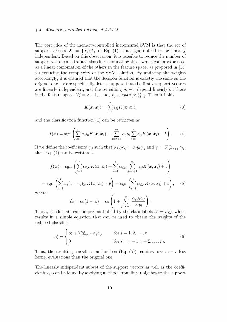
4.3 Memory-controlled Incremental SVM

The core idea of the memory-controlled incremental SVM is that the set ofsupport vectors X = {xi}

mi=1 in Eq. (1) is not guaranteed to be linearly

independent. Based on this observation, it is possible to reduce the number ofsupport vectors of a trained classifier, eliminating those which can be expressedas a linear combination of the others in the feature space, as proposed in [15]for reducing the complexity of the SVM solution. By updating the weightsaccordingly, it is ensured that the decision function is exactly the same as theoriginal one. More specifically, let us suppose that the first r support vectorsare linearly independent, and the remaining m − r depend linearly on thosein the feature space: ∀j = r + 1, . . . m, xj ∈ span{xi}

ri=1. Then it holds

K(x, xj) =r∑

i=1

cijK(x, xi), (3)

and the classification function (1) can be rewritten as

f(x) = sgn

r∑

i=1

αiyiK(x, xi) +m∑

j=r+1

αjyj

r∑

i=1

cijK(x, xi) + b

. (4)

If we define the coefficients γij such that αjyjcij = αiyiγij and γi =∑m

j=r+1 γij,then Eq. (4) can be written as

f(x) = sgn

r∑

i=1

αiyiK(x, xi) +r∑

i=1

αiyi

m∑

j=r+1

γijK(x, xi) + b

= sgn

(r∑

i=1

αi(1 + γi)yiK(x, xi) + b

)= sgn

(r∑

i=1

αiyiK(x, xi) + b

), (5)

where

αi = αi(1 + γi) = αi

1 +

m∑

j=r+1

αjyjcij

αiyi

.

The αi coefficients can be pre-multiplied by the class labels α′

i = αiyi whichresults in a simple equation that can be used to obtain the weights of thereduced classifier:

α′

i =

α′

i +∑m

j=r+1 α′

jcij for i = 1, 2, . . . , r

0 for i = r + 1, r + 2, . . . ,m.(6)

Thus, the resulting classification function (Eq. (5)) requires now m − r lesskernel evaluations than the original one.

The linearly independent subset of the support vectors as well as the coeffi-cients cij can be found by applying methods from linear algebra to the support

10

vector matrix given by

K =

K(x1, x1) · · · K(x1, xm)...

. . ....

K(xm, x1) · · · K(xm, xm)

, (7)

We employ the QR factorization with column pivoting [18] for this purpose.The QR factorization with column pivoting algorithm is a widely used methodfor selecting the independent columns of a matrix. The algorithm allows toreveal the numerical rank of the matrix with respect to a parameter τ , whichacts as a threshold in defining the condition of linear dependence. Additionally,it performs a permutation of the columns of the matrix so that they are orderedaccording to the degree of their relative linear independence. Consequently, iffor a given value of τ the rank of the matrix is r, then the linearly independentcolumns will occupy the first r positions.

The QR factorization with column pivoting of the matrix K ∈ ℜm×m is givenby

KΠ = QR, (8)

where Π ∈ ℜm×m is a permutation matrix, Q ∈ ℜm×m is orthogonal, andR ∈ ℜm×m is upper triangular. If we assume that the rank of the matrix Kwith respect to the parameter τ equals r, then the matrices can be decomposedas follows:

[K1 K2

]=[Q1 Q2

]

R11 R12

0 R22

, (9)

where the columns of K1 ∈ ℜm×r create a linearly independent set, thecolumns of K2 ∈ ℜm×m−r may be expressed as a linear combination of thecolumns of K1, Q1 ∈ ℜm×r, Q2 ∈ ℜm×m−r, R11 ∈ ℜr×r, R12 ∈ ℜr×m−r,R22 ∈ ℜm−r×m−r.

The products of the QR factorization can be used to obtain the coefficients cij

as follows

C =

c1,r+1 . . . c1,m

.... . .

...

cr,r+1 . . . cr,m

= R−1

11 QT1 K2. (10)

The coefficients together with the permutation matrix Π ∈ ℜm×m and thenumber of the linearly independent support vectors r are sufficient to obtainthe reduced solution. Using matrix notation, Eq. (6) can be expressed as fol-lows

α′

1 = α′

1 + R−1

11 QT1 K2α

′

2

α′

2 = 0(11)

11

The rank r of the matrix K can be estimated by thresholding ‖R22‖2 withthe value of the parameter τ . This means that, in practice, the choice of the τvalue determines the number of linearly independent support vectors retainedby the algorithm. For instance, by choosing a value of τ of 0.1 one will selecta number of linearly independent support vectors smaller than by choosing aτ value of 0.01. This has two concrete effects on the algorithm:

(1) As the value of τ increases, the number of support vectors decreases. Thismeans that, by tuning τ , it is possible to reduce the memory requirementsand to increase speed during classification;

(2) At the same time, as τ increases, Eq. (5) will become more and morean approximation of the exact solution, because we are considering aslinearly dependent vectors that are not. Therefore, we are not able topreserve fully their informative content. Still, we don’t lose all the infor-mation carried by the discarded support vector xj, as its weight αj isused to compute the updated value of the weights αi for the remainingsupport vectors. This should result in a graceful decrease of classificationperformance compared to the optimal solution.

We propose to combine this model simplification with the fixed-partition in-cremental algorithm, adding the reduction process at each incremental step.We call the new algorithm memory-controlled incremental SVM. It can beillustrated as follows:

(1) Train. The algorithm receives the first batch of data T 1. It trains anSVM and obtains a set of support vectors SV 1.

(2) Find linearly dependent SVs. The algorithm finds permutation ofSV 1 that orders the SVs according to the degree of their linear indepen-dence.

(3) Find τ . The algorithm searches for the value of τ , τ ⋆, that satisfies cer-tain requirements regarding the number of support vectors or estimatedperformance of the classifier.

(4) Reduce. The algorithm computes the reduced solution determined bythe chosen τ ⋆. After this step, the reduced model contains a subset of theoriginal SVs, SV 1 = red(SV 1), and can be used to classify test data.

(5) Retrain. As the new batch of data T 2 arrives, step (1) is repeated using

as training vectors Tinc

2 = {T 2 ∪ SV 1}.

For applications that require speed and/or have limited memory requirements,at step (3) of the algorithm, one can tune τ so to obtain at each incrementalstep a predefined maximum number of stored SV. For applications whereaccuracy is more relevant, one can estimate at each incremental step the τcorresponding to a pre-defined maximum decrease in performance. This canbe done on the batch of data T i at each step, dividing T i in two subsetsand training on one and testing on the other or by applying the leave-one-

12

out strategy. We denote with the symbol Θ the percentage of the originalclassification rate that is guaranteed to be preserved after the reduction inthis case.

In order to apply the method to multi-class problems, we used the one-vs-one multi-class extension. In a set of preliminary experiments comparing theone-vs-one and one-vs-all algorithms, we did not observe significant differ-ences in the behavior of both methods (for further details, we refer the readerto [37]). The one-vs-one algorithm, given M classes, trains M(M − 1)/2 two-class SVMs, one for each pair of classes. In case of the place recognition ex-periments, this method obtained smaller training times due to large numberof training samples and relatively small number of classes.

4.4 Online Independent Incremental SVM

The idea to exploit the linear independence in the feature space has alsobeen implemented in an online extension of SVMs, called Online Indepen-dent Support Vector Machine (OISVM, [36]). OISVM selects incrementallybasis vectors that are used to build the solution of the SVM training problem,based upon linear independence in the feature space. Vectors that are linearlydependent on already stored ones are rejected. An incremental minimizationalgorithm is employed to find the new minimum of the cost function. Thisapproach reduces considerably the complexity of the solution and thereforethe testing time. As OISVM is an exact method, it requires to store all dataacquired by the system during its whole life span for the update of the costfunction. In many cases (e.g. in case of place recognition), the data samplesare multi-dimensional and require a substantial amount of storage. Addition-ally, the learning algorithm needs to build a gram matrix the size of which isquadratic in the number of training samples. This leads inevitably to a mem-ory explosion when the number of incremental steps grows, as we will showexperimentally. Through its heuristics, the memory-controlled algorithm al-lows to decrease the number of training data samples at each incremental stepand thus reduce the memory consumption.

5 Experimental Setup

This section describes our experimental setup. We first describe the IDOL2and COLD-Freiburg databases, on which we will run all the experiments re-ported in this paper (Sections 5.1 and 5.2), then we briefly describe the fea-ture representations used in the experiments (Section 5.3). Finally, we discuss

13

1-person office 2-persons office Kitchen Corridor Printer area

Min

nie

Dum

bo

Fig. 3. Robot platforms employed in the experiments with the IDOL2 database andimages illustrating the appearance of the five rooms from the robots’ the point ofview.

Fig. 4. Sample images illustrating the variations captured in the IDOL2 database.Images in the top row show the variability introduced by changes in illumination fortwo rooms. The second and third rows show people appearing in the environment(first three images, second row) as well as the influence of people’s activity includingsome larger variations which happened over a time span of 6 months. Finally, thebottom row illustrates the changes in viewpoint observed for a series of imagesacquired one after another in 1.2 second.

the performance evaluation measure and parameter selection method (Sec-tion 5.4).

5.1 The IDOL2 Database

The IDOL2 (Image Database for rObot Localization 2, [29]) database con-tains 24 image sequences acquired by a perspective camera, mounted on twomobile robot platforms. Both mobile robot platforms, the PeopleBot Minnie

14

and the PowerBot Dumbo, are equipped with cameras. On Minnie the cam-era is located 98cm above the floor, whereas on Dumbo its height is 36cm.Fig. 3 shows both robots and some sample images from the database acquiredby the robots from very close viewpoints, illustrating the difference in visualcontent. These images were acquired under the same illumination conditionsand within short time spans.

The robots were manually driven through an indoor laboratory environmentand the images were acquired at a rate of 5fps. Each image sequence consists of800-1100 frames automatically labeled with one of five different classes (PrinterArea [PA], CoRridor [CR], KiTchen [KT], Two-persons Office [TO], and One-person Office [OO]). The labeling is based on the camera’s position given bythe laser-based localization system proposed in [16]. The acquisition procedurewas repeated several times to capture the changes in illumination and varyingweather conditions (sunny, cloudy, and night). Also, special care was taken tocapture people’s activities, change of location for objects and for furniture; forpart of the environment (two-persons office) we were able to record a significantchange in decoration which occurred over a time span of 6 months. Fig. 4shows some sample images from the database, illustrating these variations. Itis important to note that each single sequence captures the appearance of theconsidered experimental environment under stable illumination settings andduring the short span of time that is required to drive the robot manuallyaround the environment.

The 24 image sequences are divided as follows: for each robot platform andfor each type of illumination conditions (cloudy, sunny, night), there are foursequences recorded. Of these four sequences, the first two were acquired sixmonths before the last two. This means that, for every robot we always havesubsets of sequences acquired under similar conditions and close in time, aswell as subsets acquired under different conditions and distant in time. Thismakes the database useful for several types of experiments. It is important tonote that, even for the sequences acquired within a short time span, variationsstill exist from everyday activities and viewpoint differences during acquisition.For further details, we refer the reader to [29].

5.2 The COLD-Freiburg Database

The COLD-Freiburg database is a collection of image sequences acquired atthe Autonomous Intelligent System Laboratory at the University of Freiburgand constitutes a part of the COsy Localization Database (COLD, [39]). Theacquisition procedure of the COLD-Freiburg database was similar to that ofthe IDOL2 database. Image sequences were acquired using a mobile robot plat-form, under several illumination conditions (sunny, cloudy, night) and across

15

Corridor Large office Stairs area Printer area Kitchen (Night)

1-person office 2-persons office 1 2-persons office 2 Bathroom Kitchen (Sunny)

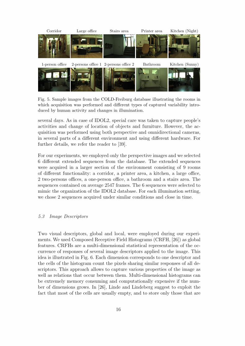
Fig. 5. Sample images from the COLD-Freiburg database illustrating the rooms inwhich acquisition was performed and different types of captured variability intro-duced by human activity and changes in illumination.

several days. As in case of IDOL2, special care was taken to capture people’sactivities and change of location of objects and furniture. However, the ac-quisition was performed using both perspective and omnidirectional cameras,in several parts of a different environment and using different hardware. Forfurther details, we refer the reader to [39].

For our experiments, we employed only the perspective images and we selected6 different extended sequences from the database. The extended sequenceswere acquired in a larger section of the environment consisting of 9 roomsof different functionality: a corridor, a printer area, a kitchen, a large office,2 two-persons offices, a one-person office, a bathroom and a stairs area. Thesequences contained on average 2547 frames. The 6 sequences were selected tomimic the organization of the IDOL2 database. For each illumination setting,we chose 2 sequences acquired under similar conditions and close in time.

5.3 Image Descriptors

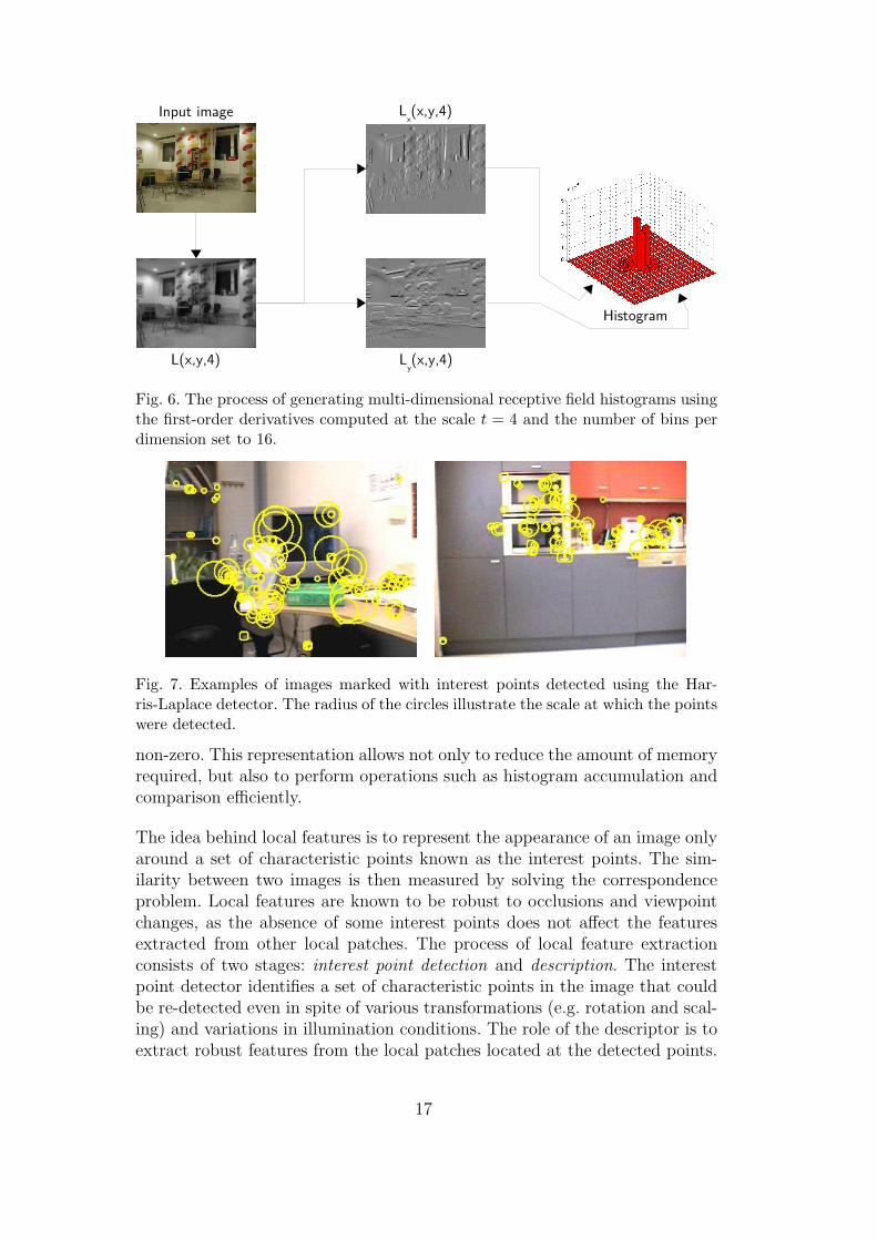
Two visual descriptors, global and local, were employed during our experi-ments. We used Composed Receptive Field Histograms (CRFH, [26]) as globalfeatures. CRFHs are a multi-dimensional statistical representation of the oc-currence of responses of several image descriptors applied to the image. Thisidea is illustrated in Fig. 6. Each dimension corresponds to one descriptor andthe cells of the histogram count the pixels sharing similar responses of all de-scriptors. This approach allows to capture various properties of the image aswell as relations that occur between them. Multi-dimensional histograms canbe extremely memory consuming and computationally expensive if the num-ber of dimensions grows. In [26], Linde and Lindeberg suggest to exploit thefact that most of the cells are usually empty, and to store only those that are

16

L(x,y,4)

Lx(x,y,4)

Ly(x,y,4)

Histogram

Input image

Fig. 6. The process of generating multi-dimensional receptive field histograms usingthe first-order derivatives computed at the scale t = 4 and the number of bins perdimension set to 16.

Fig. 7. Examples of images marked with interest points detected using the Har-ris-Laplace detector. The radius of the circles illustrate the scale at which the pointswere detected.

non-zero. This representation allows not only to reduce the amount of memoryrequired, but also to perform operations such as histogram accumulation andcomparison efficiently.

The idea behind local features is to represent the appearance of an image onlyaround a set of characteristic points known as the interest points. The sim-ilarity between two images is then measured by solving the correspondenceproblem. Local features are known to be robust to occlusions and viewpointchanges, as the absence of some interest points does not affect the featuresextracted from other local patches. The process of local feature extractionconsists of two stages: interest point detection and description. The interestpoint detector identifies a set of characteristic points in the image that couldbe re-detected even in spite of various transformations (e.g. rotation and scal-ing) and variations in illumination conditions. The role of the descriptor is toextract robust features from the local patches located at the detected points.

17

In this paper, we used the scale, rotation, and translation invariant Harris-Laplace detector [32] and the SIFT descriptor [28]. Fig. 7 shows two examplesof interest point detected on images of indoor environments.

5.4 Parameter Selection and Performance Evaluation

For all experiments, the kernel parameter and the SVM cost parameter Cwere determined via cross validation, separately for each database. Then, theobtained values were used as constants for all the incremental learning exper-iments. For all experiments, we used the implementation of SVM provided bythe libsvm library [9].

Since the employed datasets are unbalanced (e.g. in case of the IDOL2 databasethere are on average 443 samples for CR, 114 for 1pO, 129 for 2pO, 133 forKT and 135 for PR), as a measure of performance for the reported resultsand parameter selection, we used the average of classification rates obtainedseparately for each actual class. For each single experiment, the percentage ofproperly classified samples was first calculated separately for each room andthen averaged with equal weights independently of the number of samples ac-quired in the room. This allowed to eliminate the influence that large classescould have on the performance score.

In our experiments, we observed a few percent improvement of the final resultswhen a performance measure that is not invariant to unbalanced classes wasused. This was caused by very good performance of the system for the corridorclass. The was visually distinct from the other classes and was represented bythe largest number of samples. As a result, in our experiments, the measurewas used mainly to compensate for the influence of the corridor class.

6 Experiments on Support Vector Reduction

To begin with, we run some experiments to evaluate the behavior of the sup-port vector reduction algorithm described in Section 4.3. We used two se-quences from the IDOL2 database [29], one as train set and the other as testset. We chose CRFH as an image descriptor, and trained SVMs with fourdifferent types of kernels: linear kernel, RBF kernel, χ2 kernel and histogramintersection (Hist.-Inte.) kernel. First, the SVM classifier was trained using theSMO algorithm. Then, starting from the obtained discriminative function, thereduction algorithm was tested, for different values of the reduction thresholdτ . After each experiment (for each value of τ), the original model was reducedand the number of kept support vectors and the performance of the reduced

18

0 0.1 0.2 0.3 0.4 0.5 0.6 0.7 0.8 0.9 110

−7

10−6

10−5

10−4

10−3

10−2

10−1

100

Percentage of the initial number of SV [%]

τ: R

eduction thre

shold

linear kernel, SV=711

RBF kernel, SV=409

χ2 kernel, SV=416

Hist.−Inte. kernel, SV=583

80 82 84 86 88 90 92 94 96 98 10010

−7

10−6

10−5

10−4

10−3

10−2

10−1

100

Θ: Percentage of the initial classification rate [%]

linear kernel, Acc.=69.4%

RBF kernel, Acc.=91.3%

χ2 kernel, Acc.=93.0%

Hist.−Inte. kernel, Acc.=90.2%

Fig. 8. Percentage of the reduced number of Support Vectors (SV) compared tothe initial model (left), and the percentage of the original classification rate thatis preserved after the reduction (right), both as a function of different value of τ

for various kernel types. The initial number of Support vectors (SV) and initialclassification rate (Acc.) were reported for each kernel.

model were tested on the same test set. If the classification rate dropped below80% of the initial classification rate, i.e. Θ < 80%, the process was stopped.Fig. 8 reports the percentage of the reduced number of Support Vectors (SV)compared to the initial model (left), and the percentage of the initial classifica-tion rate that is preserved after the reduction (right), as a function of differentvalue of τ . We see that, apart for the linear kernel, the algorithm behaves asexpected, obtaining a gentle decrease in performance as the number of storedsupport vectors is being reduced. It is worth noting that the linear kernel isknown for being not a good metric for histogram-like features, as instead allthe other three kernels are. This might explain its different behavior.

7 Experiments on Adaptation

As a first application of our method, we present experiments on visual placerecognition in highly dynamic indoor environments. We consider a realisticscenario, where places change their visual appearance because of varying illu-mination conditions or human activity. Specifically, we focus on the ability ofthe recognition algorithm to adapt to these changes over long periods of time.As it is not possible to predict in advance the type of changes that will occur,adaptation must be performed incrementally.

We conducted two series of experiments to evaluate the effectiveness of thememory-controlled incremental SVM for this task. In the first, we considereda case in which the variability observed by the recognition system was con-strained to changes introduced by long-term human activity under stable il-lumination conditions. Such experimental procedure allowed us to thoroughly

19

examine the properties of each of the incremental methods in a more controlledsetting. The corresponding experiments are reported in Section 7.1. In the sec-ond, we considered a real-world, unconstrained scenario where the algorithmshad to incrementally gain robustness to variations introduced by changing il-lumination and short-term human activity, and then, to use their adaptationabilities to handle long-time environment changes. The corresponding exper-iments are reported in Section 7.2. In both experiments, we compared ourapproach with the fixed-partition incremental SVM, OISVM and the batchmethod. This last algorithm is used here purely as a reference, as it is notincremental. We used CRFH global image features. We tested a wide varietyof combinations of image descriptors, with several scale levels [37]. On thebasis of an evaluation of performance and computational cost, we built thehistograms from normalized Gaussian derivative filters applied to the imagesat two different scales, and we used χ2 as a kernel for SVM. We also performedexperiments using SIFT local features combined with the matching kernel forSVM. Both types of features previously proved effective for the place recogni-tion task [41,40].

7.1 Experiments with Constrained Variability

In the first series of experiments, we evaluated the properties of the memory-controlled incremental SVM in a simplified scenario. We therefore trainedthe system on three sequences acquired under similar illumination conditions,with the same robot platform. The fourth sequence was used for testing. Train-ing on each sequence was performed in 5 steps, using one subsequence at atime, resulting in 15 steps in total. We considered 36 different permutations oftraining and test sequences. Here we report average results obtained on bothglobal and local features by the three incremental algorithms (fixed-partition,OISVM, and memory-controlled) as well as the batch method. We tested thememory-controlled algorithm using two different values of the parameter Θ,i.e. Θ = 99%, 95%. This corresponds to the maximum accepted reduction ofthe recognition rate of 1% and 5% respectively, as explained in Section 4.3.Similarly for OISVM, we used three different values of the parameter η thatdetermines how sparse the final solution is going to be (as in [36]).

Fig. 9, left, shows the recognition rates obtained at each incremental stepby all methods and for both feature types. Fig. 9, right, reports the num-ber of training samples that had to be stored in the memory at each stepof the incremental procedure. First, we see that OISVM achieves very goodperformance similar to the batch method. However, both methods suffer fromthe same problem: they require all the training samples to be kept in thememory during the whole learning process. This makes them unsuitable forrealistic scenarios, particularly in cases when the algorithm should be used

20

! ∀ # ∃ % &! &∀ &# &∃∃∋

(!

(∋

%!

%∋

)!

)∋

∗+,−.−./01234

56,77−8−9,2−:.0;,230<=>

0

0

00?,29≅

00Α−Β3Χ!4,+2−2−:.

00∆3Ε:+Φ!9:.2+:663ΧΓ0!Η))=

00∆3Ε:+Φ!9:.2+:663ΧΓ0!Η)∋=

00Ιϑ1Κ∆Γ0∀Η!Λ!&

00Ιϑ1Κ∆Γ0∀Η!Λ!∀∋

! ∀ # ∃ % &! &∀ &# &∃!

∋!!

&!!!

&∋!!

∀!!!

∀∋!!

(!!!

)∗+,−,−./0123

45672∗/89/018∗2:/;2<18∗=/,−/>268∗?

/

/

//≅+1<Α

//Β,Χ2:!3+∗1,1,8−

//>268∗?!<8−1∗8∆∆2:Ε/!ΦΓΓΗ

//>268∗?!<8−1∗8∆∆2:Ε//!ΦΓ∋Η

//Ιϑ0;>Ε/∀Φ!Κ!&

//Ιϑ0;>Ε/∀Φ!Κ!∀∋

(a) Classification rate and number of training samples stored for global features.

! ∀ # ∃ % &! &∀ &# &∃∃!

∃∋

(!

(∋

%!

%∋

)!

)∋

∗+,−.−./01234

56,77−8−9,2−:.0;,230<=>

0

0

00?,29≅

00Α−Β3Χ!4,+2−2−:.

00∆3Ε:+Φ!9:.2+:663ΧΓ0!Η))=

00∆3Ε:+Φ!9:.2+:663ΧΓ0!Η)∋=

00Ιϑ1Κ∆Γ0∀Η!Λ&!

00Ιϑ1Κ∆Γ0∀Η!Λ∀!

! ∀ # ∃ % &! &∀ &# &∃!

∋!!

&!!!

&∋!!

∀!!!

∀∋!!

(!!!

)∗+,−,−./0123

45672∗/89/018∗2:/;2<18∗=/,−/>268∗?

/

/

//≅+1<Α

//Β,Χ2:!3+∗1,1,8−

//>268∗?!<8−1∗8∆∆2:Ε/!ΦΓΓΗ

//>268∗?!<8−1∗8∆∆2:Ε//!ΦΓ∋Η

//Ιϑ0;>Ε/∀Φ!Κ&!

//Ιϑ0;>Ε/∀Φ!Κ∀!

(b) Classification rate and number of training samples stored for local features.

Fig. 9. Average results obtained for the experiments with constrained variability forthree incremental methods and the batch algorithm.

on a robotic platform with intrinsically limited resources. The fixed-partitionalgorithm achieves identical performance as the batch method, while greatlyreducing the number of training samples that need to be stored in the mem-ory at each incremental step. However, despite that all the algorithms showplateaus in the classification rate whenever the model is trained on similardata (coming from consecutive subsequences), the number of support vectorsgrows roughly linearly with the number of training steps.

We see that for the memory-controlled incremental SVM, both the classifica-tion rate and the number of stored support vectors show plateaus every fiveincremental steps (as opposed to the classification rate only in case of the othermethods). The method controls the memory growth much more successfullythan the original fixed-partition incremental technique. For instance, when weaccept only one percent reduction in classification (i.e. Θ = 99%), the num-ber of support vectors stored after the 15 steps is 39.6% (CRFH) and 43.7%(SIFT) lower than for the fixed-partition incremental method. For Θ = 95%,the gain in memory compression is much greater than the overall decrease

21

in performance. This feature, i.e. the possibility to trade memory for a con-trolled reduction in performance, can be potentially very useful for systemsoperating in realistic, open-ended learning scenarios and with limited memoryresources. This approach would be even more appealing for systems which cancompensate the loss in performance by doing information fusion over time orfrom multiple sensors. It is worth underlying that the growth in the number ofsupport vectors decreases over time (Fig. 9, bottom). For example, for CRFHand Θ = 99%, the model trained on the second sequence (step 6 to 10) growsby 115 vectors on average, but trained on the third sequence (step 11 to 15)grows only by 74 vectors. This may indicate that the number of SVs eventuallytends to reach a plateau.

In order to gain a better understanding of the methods’ behavior, we per-formed an additional analysis of the results. Fig. 11b shows, for the two ap-proximate incremental techniques, the average amounts of vectors (originat-ing from each of the three training sequences) that remained in the modelafter the final incremental step (note that, in our case, this analysis would bepointless for OISVM, as it requires storing all the training data). The figureillustrates how the methods weigh instances, learned at different time, whenconstructing the internal representation. We see that both fixed-partition andmemory-controlled algorithms privilege new data, as the SVs from the lasttraining sequence are more represented in the model. This phenomenon isstronger for the memory-controlled algorithm.

To get a feeling for how the forgetting capability works in case of the memory-controlled method, we plotted the positions where the SVs were acquired, forΘ = 99% and the CRFH features. Fig. 10 reports results obtained for a modelbuilt after the final incremental step. The positions were marked on threemaps presented in Fig. 10a,b,c so that each of the maps shows the SVs orig-inating from only one training sequence. These SVs could be considered aslandmarks selected by the visual system for the recognition task. As alreadyshown in Fig. 11b, most of the vectors in the model come from the last trainingsequence. Moreover, the number of SVs from the previous training steps de-creases monotonically, thus the algorithm gradually forgets the old knowledge.It is interesting to observe how the vectors from each sequence are distributedalong the path of the robot. On each map, the places crowded with SVs aremainly transition areas between the rooms, regions of high variability, as wellas places at which the robot rotated (thus providing a lot of different visualcues without changing position). To illustrate the point, Fig. 11a shows sam-ple images acquired in the corridor, for which the SVs decay quickly, and oneof the offices, for which they are being preserved much longer. The resultsindicate that the forgetting is not performed randomly. On the contrary, thealgorithm tends to preserve those training vectors that are most crucial fordiscriminative classification, and first forgets the most redundant ones.

22

On the basis of these experimental findings, we can conclude that the memory-controlled incremental SVM is the best method for vision-based robot local-ization of those considered here. Therefore, in the rest of the paper we willuse only this algorithm, with Θ = 99%.

7.2 Experiments with Unconstrained Variability

The next step was to test our incremental method in a real-world scenario.To this purpose, we considered the case where the algorithm needed to in-crementally gain robustness to variations introduced by changing illuminationand human activities, while at the same time using its adaptation ability tohandle long-time changes in the environment. We performed the experimentsfirst on the IDOL2 database. Then, to confirm the behavior on a different setof data, we used the COLD-Freiburg database. We first trained the systemon three IDOL2 sequences acquired at roughly similar time but under differ-ent illumination conditions. Then, we repeated the same training procedureon sequences acquired 6 months later. In order to increase the number of in-cremental steps and differentiate the amount of new information introducedby each set of data, each sequence was again divided into five subsequences.In total, for each experiment we performed 30 incremental steps. Since theIDOL2 database consists of pairs of sequences acquired under roughly similarconditions, each training sequence has a corresponding one which could beused for testing. Feature-wise, here we used only the global features (CRFH).Indeed, the experiments presented in the previous section showed that localfeatures achieve an accuracy similar to that of CRFH, but at a much highercomputational cost and memory requirement. Also, preliminary experimentsshow that this behavior is confirmed in this scenario, hence the choice to usehere only the global descriptor.

We used a very similar system and experimental procedure for the exper-iments with the COLD-Freiburg dataset. As in case of IDOL2, we dividedeach sequence into 5 subsequences and used pairs of sequences acquired underroughly similar conditions for training and testing. In case of both databases,the experiment was repeated 12 times for different orderings of training se-quences. Fig. 12 and 13 report the average results together with standarddeviations. By observing the classification rates for a classifier trained on thefirst sequence only, we see that the system achieves best performance on a testset acquired under similar conditions. The classification rate is significantlylower for other test sets. In case of IDOL2, this is especially visible for im-ages acquired 6 months later, even under similar illumination conditions. Atthe same time, the performance greatly improves when incremental learningis performed on new batches of data. The classification rate decreases for theold test sets; at the same time, the size of the model tends to stabilize.

23

(a) 78 Support Vectors from 1st seq. (b) 111 Support Vectors from 2nd seq.

(c) 149 Support Vectors from 3rd seq.

Fig. 10. Maps of the environ-ment with plotted positions ofthe support vectors stored inthe model obtained after thefinal incremental step for oneof the experiments conductedusing the memory-controlledtechnique with Θ = 99%. Thesupport vectors were dividedinto three maps (a, b, andc) according to the trainingsequence they originate from.Additionally, each map showsthe path of the robot duringacquisition of the sequence (ar-rows indicate the direction ofdriving). We observe that theSupport Vectors from the oldtraining sequences were grad-ually eliminated by the al-gorithm and this effect wasstronger in regions with lowervariability.

24

1st seq. 2nd seq. 3rd seq.

Offi

ceC

orri

dor

(a) Sample images from the

three training sequences.

!∀#∃%!&∋()∀)∀∗+ ,∃−∗(.!/∗+)(∗00∃%122345

655

755

855

955

:55

;55

<55

=55

>?−≅∃(Α∗ΒΑΧ?&&∗()Α∆∃/)∗(Ε

768

799

727

65=

695

766

Α

Α

ΑΦ(ΓΑΕ∃Η?∃+/∃Α6 ΑΦ(ΓΑΕ∃Η?∃+/∃Α7 ΑΦ(ΓΑΕ∃Η?∃+/∃Α8

(b) Statistics of Support Vectorsstored in the final approximate

incremental models.

Fig. 11. Sample images captured in regions of different variability (left). Comparisonof the average amounts of training vectors coming from the three sequences thatwere stored in the final incremental model for the two approximate incrementaltechniques (right).

! ∀ #! #∀ ∃! ∃∀ %!!

∃!!

&!!

∋!!

(!!

#!!!

#∃!!

#&!!

#∋!!

#(!!

∃!!!

)∗+,−,−./0123

45672∗/89/05338∗1/:2;18∗<

/

/

//=+1;>

//?268∗≅!;8−1∗8ΑΑ2Β

Tr. Seq. 1 Tr. Seq. 2 Tr. Seq. 3 Tr. Seq. 4 Tr. Seq. 5 Tr. Seq. 650

55

60

65

70

75

80

85

90

95

100

Cla

ssific

ation R

ate

(%

)

Memory−controlled

Testing sequence 1

Testing sequence 2

Testing sequence 3

Testing sequence 4

Testing sequence 5

Testing sequence 6

(a) Support vectors (b) Performance of memory-reduced

Fig. 12. Average results of the IDOL2 experiments in the real-world scenario. (a)compares the amounts of SVs stored in the models at each incremental step for thebatch and the memory-controlled method. (b) reports the classification rate mea-sured every fifth step (every time the system completes learning a whole sequence)with all the available test sets. The training and test sets marked with the sameindices were acquired under similar conditions.

7.3 Discussion

The presented results provide a clear evidence of the capability of the dis-criminative methods to perform incremental learning for vision-based placerecognition, and their adaptability to variations in the environment. Table 1summarizes the performance obtained by each method in terms of accuracy,speed, controlled memory growth and forgetting capability. For each algo-rithm (i.e. for each row), we put a cross corresponding to the property (i.e.

25

1 2 3 4 5 6 7 8 9 10 11 12 13 14 150

500

1000

1500

2000

2500

3000

3500

4000

4500

5000

5500

Training Step

Nu

mb

er

of

Su

pp

ort

Ve

cto

rs

Batch

Memory−controlled

1 2 3 4 5 6 7 8 9 10 11 12 13 14 1530

40

50

60

70

80

90

100

Training Step

Cla

ssific

atio

n R

ate

(%

)

Memory−controlled

Testing sequence 1

Testing sequence 2

Testing sequence 3

(a) Support vectors (b) Performance of memory-reduced

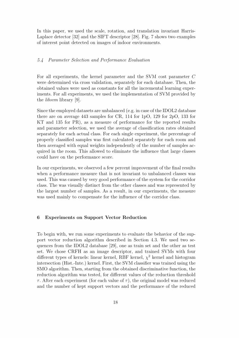
Fig. 13. Average results of the COLD-Freiburg experiments in the real-world sce-nario. (a) compares the amounts of SVs stored in the models at each incrementalstep for the batch and the memory-controlled method. (b) reports the classificationrate measured every step with all the available test sets. The consecutive trainingand testing sequences were acquired under similar conditions.

the column) that the algorithm has shown to possess in our experiments.The fixed-partition method performs as well as batch SVM, but it is unableto control the memory growth and requires much more memory space. Wealso found that OISVM could get very good accuracy while achieving a lowcomputational complexity during testing. However, none of the two methodshas shown to possess an effective forgetting capability: for the fixed-partitionmethod, the old SVs decay slowly, but the decay is neither predictable norcontrollable; for OISVM, every training vector must be stored into memory.As opposed to this, the memory-controlled algorithm is able to achieve perfor-mances statistically equivalent to those of batch SVM, while at the same timeproviding a principled and effective way to control the memory growth. Exper-iments showed that this has induced a forgetting capability which privilegesnewly acquired data to the expenses of old one and the model growth slowsdown whenever new data are similar to those already processed. Furthermore,since a lot of training images can be discarded during the incremental process,the training time soon becomes significantly lower than for the batch method.For instance, in case of the second experiments, training the classifier at thelast step took 25.5s for the batch algorithm and only 5.6s for the memory-controlled method on a 2.6GHZ Pentium IV machine, and recognition timewas twice as fast for the memory-controlled algorithm than for the batch one.

26

Accuracy Forgetting Memory Speed

Fixed-partition x x

OISVM x x

Memory-controlled x x x x

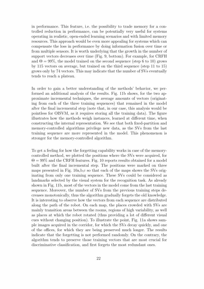
Table 1Comparing incremental learning techniques for place recognition and robot local-ization applications.

KnowledgeTransferred

Across Platforms

TrainingTraining TrainingSVReduction

TrainingTraining

Traing Set 1 Traing Set 2 Traing Set N

Testing Testing

SVMModel

SVMModel

SVsSVsSVs

Fig. 14. A diagram illustrating the data flow in the knowledge-transfer system.

8 Experiments on Knowledge Transfer

As a second application of our method, we considered the problem of trans-fer of knowledge between robotic platforms with different characteristics, per-forming vision-based recognition in the same environment. We used the IDOL2database and the robots Minnie and Dumbo for these experiments. The maindifference between the two platforms lies in the height of the cameras (seeFig. 15). They both use the memory-controlled incremental SVM as a basisfor their recognition system, thus they share the same knowledge representa-tion. The aim is to efficiently exploit the knowledge acquired e.g. by one robotso to boost the recognition performance of another robot. We propose to useour method to update the internal representation when new training dataare available. Fig. 14 illustrates how our approach can be used for transferof knowledge. We would like the knowledge transfer scheme to be adaptive,and also to privilege newest data so to avoid accumulation of outdated in-formation. Finally, the solution obtained starting from a transferred modelshould gradually converge to the one learned from scratch, not only in termsof performance but also of required resources (e.g. memory).

The challenges in the transfer of knowledge will come from:

• (a) Differences in the parameters of the two platformsThe cameras are mounted at two different heights, thus the informativecontent of the images acquired by the two platforms is different. Because ofthis, the knowledge acquired by one platform might not be helpful for theother one or, in the worst case, it might constitute an obstacle. Preliminaryexperiments showed that SIFT is more suitable for the transfer of knowledge

27

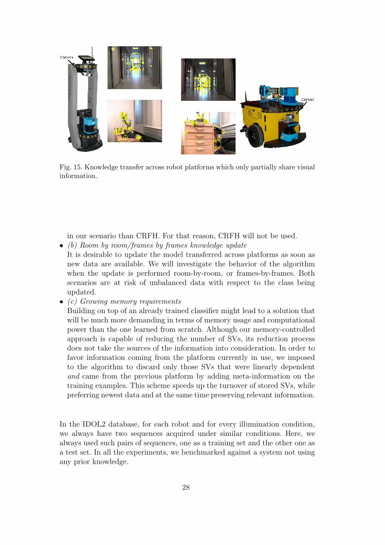
Fig. 15. Knowledge transfer across robot platforms which only partially share visualinformation.

in our scenario than CRFH. For that reason, CRFH will not be used.• (b) Room by room/frames by frames knowledge update

It is desirable to update the model transferred across platforms as soon asnew data are available. We will investigate the behavior of the algorithmwhen the update is performed room-by-room, or frames-by-frames. Bothscenarios are at risk of unbalanced data with respect to the class beingupdated.

• (c) Growing memory requirementsBuilding on top of an already trained classifier might lead to a solution thatwill be much more demanding in terms of memory usage and computationalpower than the one learned from scratch. Although our memory-controlledapproach is capable of reducing the number of SVs, its reduction processdoes not take the sources of the information into consideration. In order tofavor information coming from the platform currently in use, we imposedto the algorithm to discard only those SVs that were linearly dependentand came from the previous platform by adding meta-information on thetraining examples. This scheme speeds up the turnover of stored SVs, whilepreferring newest data and at the same time preserving relevant information.

In the IDOL2 database, for each robot and for every illumination condition,we always have two sequences acquired under similar conditions. Here, wealways used such pairs of sequences, one as a training set and the other one asa test set. In all the experiments, we benchmarked against a system not usingany prior knowledge.

28

8.1 Experiments with room by room updates

In the first series of experiments, the system was updated incrementally in aroom by room (i.e. class by class) scenario. The system was trained incremen-tally on one sequence; the corresponding sequence, acquired under roughlysimilar conditions, was used for testing. The prior-knowledge model was builtusing standard batch SVM from one image sequence, acquired under the sameillumination conditions and at close time as the training one, but using a dif-ferent platform. As there are five classes in total, training was performed in5 steps (the algorithm learned incrementally one room at the time). In theno-transfer case, the system needed to build the model from scratch, and thusneeded to acquire data from at least two classes. In this case, training on eachsequence required only 4 steps since in the first step the algorithm learned todistinguish between the first two classes.

Building on top of knowledge acquired from another platform implies a growthin the memory requirements. To evaluate this behavior in relationship to itseffects on performance and compare fairly to the system trained without aprior model, we incrementally updated the model without transferred knowl-edge on another sequence acquired under conditions similar to that of the firsttraining sequence. This experiment makes it possible to evaluate performanceand memory growth when both systems are trained on two sequences. Themain difference is that in one case both sequences were acquired and pro-cessed by the same platform; in the other case, one sequence was acquired andprocessed by a different platform. We considered different permutations in therooms order for the updating; for each permutation, we considered 6 differentorderings of the sequences used as training, testing, and prior-knowledge sets.Due to space reasons, we report only average results for one permutation,together with standard deviations in Fig. 16.

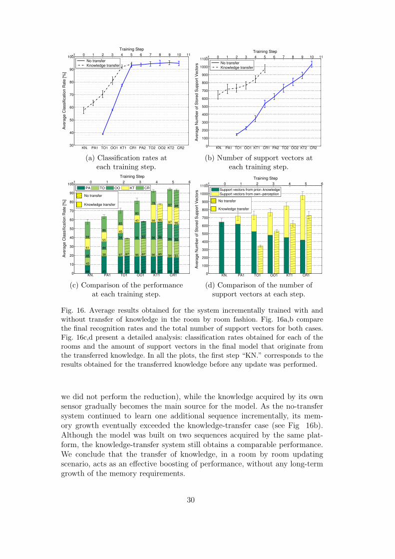
We can see that, for both approaches, the system gradually adapts to its ownperception of the environment. It is clear that the knowledge-transfer systemhas a great advantage in terms of performance over the no-transfer system atthe first steps. For instance, we see that, after the second update (TO1, Fig16a), the knowledge-transfer system achieves a classification rate of 65.3%,while the no-transfer knowledge obtains only 37%. The advantage in classi-fication rate for the knowledge-transfer system remains considerable for thesteps OO1 and KT1. However, it is interesting to note that even when bothsystems have been updated on a full sequence (CR1, Fig 16a), the knowledge-transfer system still maintains an advantage in performance. Considering thedifferences between the two platforms, and that the transferred knowledgemodel was built on a single sequence, this is a remarkable result. It can alsobe observed from Fig. 16d that the memory-controlled algorithm facilitatedthe decay of knowledge from the other platform (in the first incremental step,

29

−1 0 1 2 3 4 5 6 7 8 9 10 11

30

40

50

60

70

80

90

100

KN. PA1 TO1 OO1 KT1 CR1 PA2 TO2 OO2 KT2 CR2

Training Step

Avera

ge C

lassific

ation R

ate

[%

]

No transfer

Knowledge transfer

−1 0 1 2 3 4 5 6 7 8 9 10 11

0

100

200

300

400

500

600

700

800

900

1000

1100

KN. PA1 TO1 OO1 KT1 CR1 PA2 TO2 OO2 KT2 CR2

Training Step

Avera

ge N

um

ber

of S

tore

d S

upport

Vecto

rs

No transfer

Knowledge transfer

(a) Classification rates ateach training step.

(b) Number of support vectors ateach training step.

−1 0 1 2 3 4 5 6

0

10

20

30

40

50

60

70

80

90

100

Training Step

KN. PA1 TO1 OO1 KT1 CR1

No transfer

Knowledge transfer

44

43

45

61

94

95

38

44

55

86

94

97

34

45

83

93

96

96

40

80

93

96

96

98

78

89

94

94

97

97

97

97

97

97

97

95

88

91

97 9692

9996

98

Avera

ge C

lassific

ation R

ate

[%

]

PA TO OO KT CR−1 0 1 2 3 4 5 6

0

100

200

300

400

500

600

700

800

900

1000

1100

Training Step

No transfer

Knowledge transfer

KN. PA1 TO1 OO1 KT1 CR1

Ave

rag

e N

um

be

r o

f S

tore

d S

up

po

rt V

ecto

rs

Support vectors from prior−knowledge

Support vectors from own−perception

(c) Comparison of the performanceat each training step.

(d) Comparison of the number ofsupport vectors at each step.

Fig. 16. Average results obtained for the system incrementally trained with andwithout transfer of knowledge in the room by room fashion. Fig. 16a,b comparethe final recognition rates and the total number of support vectors for both cases.Fig. 16c,d present a detailed analysis: classification rates obtained for each of therooms and the amount of support vectors in the final model that originate fromthe transferred knowledge. In all the plots, the first step “KN.” corresponds to theresults obtained for the transferred knowledge before any update was performed.

we did not perform the reduction), while the knowledge acquired by its ownsensor gradually becomes the main source for the model. As the no-transfersystem continued to learn one additional sequence incrementally, its mem-ory growth eventually exceeded the knowledge-transfer case (see Fig 16b).Although the model was built on two sequences acquired by the same plat-form, the knowledge-transfer system still obtains a comparable performance.We conclude that the transfer of knowledge, in a room by room updatingscenario, acts as an effective boosting of performance, without any long-termgrowth of the memory requirements.

30

0 5 10 15 20 25 30 35 40

20

25

30

35

40

45

50

55

60

65

70

75

80

85

90

95

100

Training Step

Cla

ssific

ation R

ate

[%

]

No transfer

Knowledge transfer

0 5 10 15 20 25 30 35 40

0

300

600

900

1200

Training Step

Num

ber

of S

tore

d S

upport

Vecto

rs

No transfer

Knowledge transfer

(a) Classification rates ateach training step.

(b) Number of support vectors ateach training step.

0 5 10 15 20 25 30 35

0

10

20

30

40

50

60

70

80

90

100

Training Step

Cla

ssific

atio

n R

ate

[%

]

No transfer

Knowledge transfer

KN.

PA1PA2

PA3PA4

PA5CR1CR2CR3CR4TO

1TO

2TO

3TO

4TO

5CR5CR6CR7OO1OO2OO3OO4CR8CR9CR10

CR11

CR12

CR13

KT1KT2

KT3KT4

KT5CR14

CR15

PA CR TO OO KT

(c) Detailed comparison of the performance of the system with and withoutknowledge-transfer.

0 5 10 15 20 25 30 35

0

200

400

600

800

1000

1200 No transfer

Knowledge transfer

Training Step

Num

ber

of S

tore

d S

upport

Vecto

r

KN.

PA1PA2

PA3PA4

PA5CR1CR2CR3CR4TO

1TO

2TO

3TO

4TO

5CR5CR6CR7OO1OO2OO3OO4CR8CR9CR10

CR11

CR12

CR13

KT1KT2

KT3KT4

KT5CR14

CR15

Support vectors from prior−knowledge

Support vectors from own−perception

(d) Number of stored support vectors of incremental experiment with and withoutknowledge-transfer at each step.

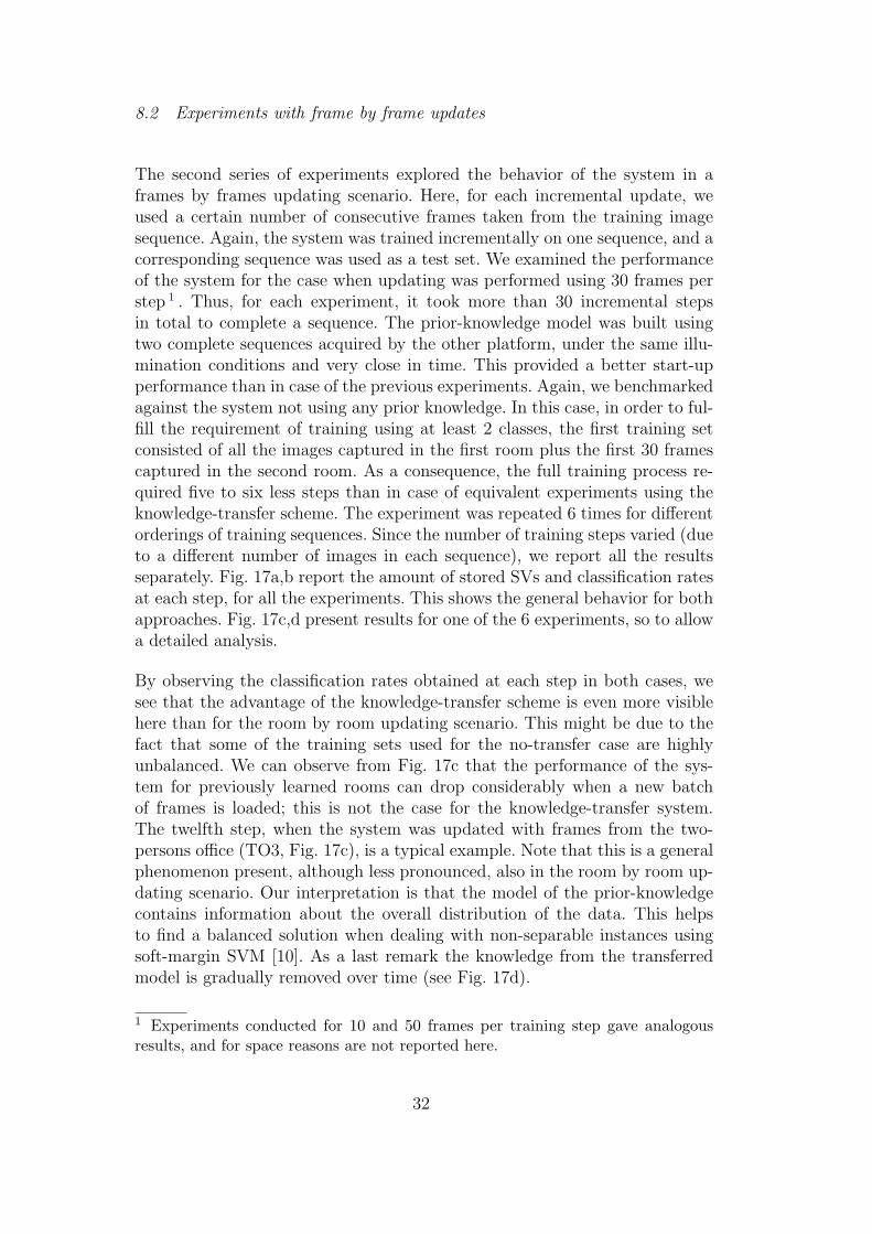
Fig. 17. Average results obtained for the system incrementally trained with andwithout transfer of knowledge in the frames by frames fashion. The labels beloweach bar indicate the batch of data used for the incremental update. Again, thefirst step labeled as “KN.” corresponds to the results obtained for the transferredknowledge before any update was performed.

31

8.2 Experiments with frame by frame updates

The second series of experiments explored the behavior of the system in aframes by frames updating scenario. Here, for each incremental update, weused a certain number of consecutive frames taken from the training imagesequence. Again, the system was trained incrementally on one sequence, and acorresponding sequence was used as a test set. We examined the performanceof the system for the case when updating was performed using 30 frames perstep 1 . Thus, for each experiment, it took more than 30 incremental stepsin total to complete a sequence. The prior-knowledge model was built usingtwo complete sequences acquired by the other platform, under the same illu-mination conditions and very close in time. This provided a better start-upperformance than in case of the previous experiments. Again, we benchmarkedagainst the system not using any prior knowledge. In this case, in order to ful-fill the requirement of training using at least 2 classes, the first training setconsisted of all the images captured in the first room plus the first 30 framescaptured in the second room. As a consequence, the full training process re-quired five to six less steps than in case of equivalent experiments using theknowledge-transfer scheme. The experiment was repeated 6 times for differentorderings of training sequences. Since the number of training steps varied (dueto a different number of images in each sequence), we report all the resultsseparately. Fig. 17a,b report the amount of stored SVs and classification ratesat each step, for all the experiments. This shows the general behavior for bothapproaches. Fig. 17c,d present results for one of the 6 experiments, so to allowa detailed analysis.

By observing the classification rates obtained at each step in both cases, wesee that the advantage of the knowledge-transfer scheme is even more visiblehere than for the room by room updating scenario. This might be due to thefact that some of the training sets used for the no-transfer case are highlyunbalanced. We can observe from Fig. 17c that the performance of the sys-tem for previously learned rooms can drop considerably when a new batchof frames is loaded; this is not the case for the knowledge-transfer system.The twelfth step, when the system was updated with frames from the two-persons office (TO3, Fig. 17c), is a typical example. Note that this is a generalphenomenon present, although less pronounced, also in the room by room up-dating scenario. Our interpretation is that the model of the prior-knowledgecontains information about the overall distribution of the data. This helpsto find a balanced solution when dealing with non-separable instances usingsoft-margin SVM [10]. As a last remark the knowledge from the transferredmodel is gradually removed over time (see Fig. 17d).

1 Experiments conducted for 10 and 50 frames per training step gave analogousresults, and for space reasons are not reported here.

32

9 Summary and Conclusions

In this paper we presented a novel extension of SVM to incremental learn-ing that achieves the same recognition performance of the standard, batchmethod while limiting the memory growth over time. This is achieved by dis-carding, at each incremental step, all the support vectors that are not linearlyindependent. The information they carry is not lost, as it is retained into thealgorithm’s decision function in the form of weighting coefficients of the re-maining support vectors. We call this method memory-controlled incrementalSVM. We applied it to the problem of place recognition for robot topolog-ical localization, focusing on two distinct scenarios: adaptation in presenceof dynamic changes and transfer of knowledge between two robot platformsengaged in the same task. Experiments show clearly the effectiveness of ourapproach in terms of accuracy, speed, reduced memory and capability to forgetredundant, outdated information.

We plan to extend this work in several ways. First, we want to use thememory-controlled algorithm in multi-modal learning scenarios, for instanceusing laser-based features combined with visual ones, as done in [41], in anincremental setting. Here we should be able to exploit fully the properties ofthe method, and aggressively trade memory for accuracy on single modalities,while retaining an high overall performance. Second, we would like to investi-gate further the knowledge transfer scenario, and incorporate in our frameworkways to select the data to be transferred, as proposed in [25]. Future work willconcentrate in these directions.

Acknowledgments

This work was sponsored by the EU FP7 project CogX (A. Pronobis) andIST-027787 DIRAC (B. Caputo, L. Jie), and the Swedish Research Councilcontract 2005-3600-Complex (A. Pronobis). The support is gratefully acknowl-edged.

References

[1] COGNIRON: The cognitive robot companion. Website:http://www.cogniron.org.

[2] CoSy: Cognitive Systems for Cognitive Assistants. Website:http://www.cognitivesystems.org/.

[3] RobotCub. Website: http://www.robotcub.org/.

33

[4] M. Artac, M. Jogan, and A. Leonardis. Mobile robot localization using anincremental eigenspace model. In Proc. ICRA’02.

[5] S. Belongie, C. Fowlkes, Chun F., and J. Malik. Spectral partitioning withindefinite kernels using the nystrom extension. In Proc. of ECCV’02.

[6] Emma Brunskill, Thomas Kollar, and Nicholas Roy. Topological mappingusing spectral clustering and classification. In Proceedings of the IEEE/RSJInternational Conference on Intelligent Robots and Systems (IROS), San Diego,October 2007.

[7] B. Caputo, E. Hayman, and P. Mallikarjuna. Class-specific materialcategorisation. In Proc. ICCV’05.

[8] G. Cauwenberghs and T. Poggio. Incremental and decremental support vectormachine learning. In Proc. NIPS’00.

[9] Chih Chung Chang and Chih Jen Lin. LIBSVM: A Library for Support VectorMachines, 2001. Available at http://www.csie.ntu.edu.tw/~cjlin/libsvm.

[10] N. Cristianini and J. S. Taylor. An introduction to support vector machines andother kernel-based learning methods. Cambridge University Press, 2000.

[11] A. Leonardis D. Skocaj. Weighted and robust incremental method for subspacelearning. In Proc. ICCV’03.

[12] M. Dissanayake, P. Newman, S. Clark, H.F. Durrant-Whyte, and M. Csorba. Asolution to the simultaneous localization and map building (SLAM) problem.IEEE Transactions on Robotics and Automation, 17(3):229–241, 2001.

[13] C. Domeniconi and D. Gunopulos. Incremental support vector machineconstruction. In Proc. ICDM’01.

[14] Gyuri Dorko and Cordelia Schmid. Object class recognition using discriminativelocal features. 2005.

[15] Tom Downs, Kevin E. Gates, and Annette Masters. Exact simplification ofsupport vector solutions. J. Mach. Learn. Res., 2, 2002.

[16] J. Folkesson, P. Jensfelt, and H. Christensen. Vision SLAM in the measurementsubspace. In Proceedings of the IEEE International Conference on Robotics andAutomation (ICRA’05), pages 30–35, Barcelona, Spain, 2005.

[17] M. Fritz, B. B. Leibe, B. Caputo, and B. Schiele. Integrating representativeand discriminant models for object category detection. In Proc. ICCV’05.

[18] G. H. Golub and C. F. Van Loan. Matrix Computations. Johns HopkinsUniversity Press, 3rd edition, 1996.

[19] M. Jogan and A. Leonardis. Robust localization using an omnidirectionalappearance-based subspace model of environment. Robotics and AutonomousSystems, 45(1):51–72, October 2003.

34

[20] T. Darrel K. Grauman. The pyramid match kernel: discriminative classificationwith sets of image features. In Proc. ICCV’05.

[21] George Konidaris and Andrew G. Barto. Autonomous shaping: knowledgetransfer in reinforcement learning. In Proc. of ICML’06.

[22] D. Kortenkamp and T. Weymouth. Topological mapping for mobile robots usinga combination of sonar and vision sensing. In Proceedings of the 12th NationalConference on Artificial Intelligence, Seattle, Washington, USA, 1994.

[23] Geert-Jan M. Kruijff, Hendrik Zender, Patric Jensfelt, and Henrik I.Christensen. Situated dialogue and spatial organization: What, where... andwhy? International Journal of Advanced Robotic Systems (ARS), Special Issueon Human-Robot Interaction, 4(1):125–138, March 2007.

[24] B. Kuipers and P. Beeson. Bootstrap learning for place recognition.In Proceedings of the 18th National Conference on Artificial Intelligence(AAAI’02), 2002.

[25] A. Lazarich, M. Restelli, and A. Bonarini. Transfer of samples in batchreinforcement learning. In Proc. ICML08.

[26] O. Linde and T. Lindeberg. Object recognition using composed receptive fieldhistograms of higher dimensionality. In Proceedings of the 17th InternationalConference on Pattern Recognition (ICPR’04), Cambridge, UK, 2004.

[27] D. G. Lowe. Distinctive image features from scale-invariant keypoints. Int. J.Computer Vision, 60(2):91–110, 2004.

[28] D. G. Lowe. Distinctive image features from scale-invariant keypoints.International Journal of Computer Vision, 60(2):91–110, 2004.

[29] J. Luo, A. Pronobis, B. Caputo, and P. Jensfelt. The IDOL2database. Technical Report 304, CVAP, KTH, 2006. Available athttp://cogvis.nada.kth.se/IDOL2/.

[30] Jr. Malak, R.J. and P. K. Khosla. A framework for the adaptive transfer of robotskill knowledge using reinforcement learning agents. In Proc. of ICRA’01.

[31] O. Martınez Mozos, R. Triebel, P. Jensfelt, A. Rottmann, and W. Burgard.Supervised semantic labeling of places using information extracted from sensordata. Robotics and Autonomous Systems, 55(5), 2007.

[32] K. Mikolajczyk and C. Schmid. Indexing based on scale invariant interest points.In Proceedings of the 8th IEEE International Conference on Computer Vision(ICCV’01), Vancouver, Canada, 2001.

[33] Tom Mitchell. The discipline of machine learning. Technical Report CMU-ML-06-108, CMU, 2006.

[34] A. C. Murillo, J. Kosecka, J. J. Guerrero, and C. Sagues. Visual door detectionintegrating appearance and shape cues. Robotics and Autonomous Systems,56(6):pp. 512–521, June 2008.

35

[35] Illah Nourbakhsh, Rob Powers, and Stan Birchfield. Dervish: An officenavigation robot. AI Magazine, 16(2):53–60, 1995.

[36] F. Orabona, C. Castellini, B. Caputo, J. Luo, and G. Sandini. Indoor placerecognition using online independent support vector machines. In 18th BritishMachine Vision Conference (BMVC07), Warwick, UK, September 2007.

[37] A. Pronobis. Indoor place recognition using support vector machines. Master’sthesis, NADA/CVAP, Kungliga Tekniska Hoegskolan, Stockholm, Sweden,December 2005.

[38] A. Pronobis and B. Caputo. Confidence-based cue integration for visual placerecognition. In Proceedings of the IEEE/RSJ International Conference onIntelligent Robots and Systems (IROS’07), San Diego, CA, USA, October 2007.

[39] A. Pronobis and B. Caputo. COLD: COsy Localization Database. TheInternational Journal of Robotics Research (IJRR), 28(5), May 2009.

[40] A. Pronobis, B. Caputo, P. Jensfelt, and H. I. Christensen. A discriminativeapproach to robust visual place recognition. In Proceedings of the IEEE/RSJInternational Conference on Intelligent Robots and Systems (IROS’06), Beijing,China, October 2006.

[41] A. Pronobis, O. Martınez Mozos, and B. Caputo. SVM-based discriminativeaccumulation scheme for place recognition. In Proceedings of the IEEEInternational Conference on Robotics and Automation (ICRA’08), Pasadena,CA, USA, May 2008.

[42] S. Se, D. G. Lowe, and J. Little. Vision-based mobile robot localizationand mapping using scale-invariant features. In Proceedings of the IEEEInternational Conference on Robotics and Automation (ICRA’01), 2001, Seoul,Korea.

[43] Christian Siagian and Laurent Itti. Biologically-inspired robotics vision monte-carlo localization in the outdoor environment. In Proceedings of the IEEE/RSJInternational Conference on Intelligent Robots and Systems (IROS’07), SanDiego, CA, USA, October 2007.

[44] Christian Siagian and Laurent Itti. Biologically-inspired robotics vision monte-carlo localization in the outdoor environment. In Proceedings of the IEEE/RSJInternational Conference on Intelligent Robots and Systems (IROS’07), SanDiego, CA, USA, October 2007.

[45] N. A. Syed, H. Liu, and K. K. Sung. Incremental learning with support vectormachines. In Proc. IJCAI’99.

[46] A. Tapus and R. Siegwart. Incremental robot mapping with fingerprints ofplaces. In Proceedings of the IEEE/RSJ International Conference on IntelligentRobots and Systems (IROS’05), Edmonton, Alberta, Canada, August 2005.

[47] Sebastian Thrun. Learning metric-topological maps for indoor mobile robotnavigation. Artificial Intelligence, 1999(1), 1998.

36

[48] Sebastian Thrun and Tom Mitchell. Lifelong robot learning. Robotics andAutonomous Systems 15, 1995.

[49] A. Torralba, K. P. Murphy, W. T. Freeman, and M. A. Rubin. Context-basedvision system for place and object recognition. In Proceedings of the IEEEInternational Conference on Computer Vision (ICCV’03), 2003, Nice, France.

[50] I. Ulrich and I. Nourbakhsh. Appearance-based place recognition for topologicallocalization. In Proceedings of the IEEE International Conference on Roboticsand Automation (ICRA’00), San Francisco, CA, USA, 2000.

[51] Christoffer Valgren and Achim J. Lilienthal. SIFT, SURF and seasons: Long-term outdoor localization using local features. In Proceedings of the EuropeanConference on Mobile Robots (ECMR’07), 2007.

[52] V. Vapnik. Statistical learning theory. Wiley and Son, 1998.

[53] C. Wallraven, B. Caputo, and A. Graf. Recognition with local features: thekernel recipe. In Proc. of ICCV’03.

[54] J. Wolf, W. Burgard, and H. Burkhardt. Robust vision-based localizationby combining an image retrieval system with monte carlo localization. IEEETransactions on Robotics, 21(2):208–216, 2005.

37