the mouse training company - mike barrett learns …microsoftproducttraining.com/documents/office...
TRANSCRIPT

The Mouse Training Company
Excel 2007Introduction
Author: Steve Moffat version 1.1 supercedes all previous versionsUpdated: 21/05/2010 16:09:58

TABLE OF CONTENTSTABLE OF CONTENTS...............................................................................................3
INTRODUCTION.......................................................................................................................... 7How To Use This Guide..................................................................................................................7Objectives......................................................................................................................................7Instructions....................................................................................................................................7
SECTION 1 THE BASICS............................................................................................8WINDOWS CONCEPTS................................................................................................................. 8
Menus............................................................................................................................................9Ribbons..........................................................................................................................................9Office Button...............................................................................................................................11Toolbars.......................................................................................................................................11Name Box....................................................................................................................................12Formula Bar.................................................................................................................................12Worksheets.................................................................................................................................12Status Bar....................................................................................................................................12Task Pane.....................................................................................................................................13Smart Tags...................................................................................................................................13
GETTING HELP........................................................................................................................... 14MICROSOFT EXCEL HELP............................................................................................................ 14
SECTION 2 MOVE AROUND AND ENTER INFORMATION........................................15MOVING................................................................................................................................... 15
Moving Around Workbook..........................................................................................................15Scrolling.......................................................................................................................................15
USEFUL KEYS FOR MOVING....................................................................................................... 16Workbook Sheets........................................................................................................................17Moving Around Sheet..................................................................................................................17
DATA ENTRY............................................................................................................................. 18Enter Text And Numbers.............................................................................................................18Cancelling And Editing Data Entries.............................................................................................18Enter Dates..................................................................................................................................19Autocomplete..............................................................................................................................20Pick From List...............................................................................................................................20
EDITING.................................................................................................................................... 21Typing Replaces Selection............................................................................................................21Use The Mouse To Edit................................................................................................................21Using The Keyboard.....................................................................................................................22Select Information.......................................................................................................................22Select Multiple Sheets.................................................................................................................23Select Non-Adjacent Sheets.........................................................................................................23
CLEAR CONTENTS, FORMATS AND COMMENTS.........................................................................24THE FILL HANDLE...................................................................................................................... 25USEFUL INFORMATION............................................................................................................. 25
Scrolling.......................................................................................................................................25Data Entry....................................................................................................................................25Select Cells To Limit Data Entry...................................................................................................26Select Cells For Multiple Entry.....................................................................................................26

SECTION 3 FORMULAE AND FUNCTIONS...............................................................27FORMULAE............................................................................................................................... 27
Typing Formulae..........................................................................................................................27Entering Formulae By Pointing....................................................................................................28Errors In Formulae.......................................................................................................................29Filling Formulae...........................................................................................................................29The Fill Handle And Formulae......................................................................................................30Fill Formulae Using Keystrokes....................................................................................................31BODMAS With Formulae.............................................................................................................31
FUNCTIONS............................................................................................................................... 32Sum Function...............................................................................................................................32Autosum......................................................................................................................................32Other Common Functions...........................................................................................................33Function Library...........................................................................................................................33Insert Function............................................................................................................................34Function Box................................................................................................................................35Type Functions............................................................................................................................35Function Argument Tool Tips.......................................................................................................35
CELL REFERENCES...................................................................................................................... 36Counting And Totalling Cells Conditionally..................................................................................36Use Sumif()..................................................................................................................................37Use Countif..................................................................................................................................38
ABSOLUTE AND RELATIVE REFERENCES.....................................................................................39Relative References.....................................................................................................................39Absolute References....................................................................................................................39Fill Handle....................................................................................................................................40Absolute References....................................................................................................................40
SECTION 4 FILE OPERATIONS.................................................................................41Save Files.....................................................................................................................................41File Types And File Names...........................................................................................................42Saving Changes To Files...............................................................................................................43Saving As A Different Type Or Different Name............................................................................43Close Files....................................................................................................................................44Open Files....................................................................................................................................45New Files.....................................................................................................................................45
SECTION 5.............................................................................................................47MOVING AND COPYING DATA...................................................................................................47
Moving Items...............................................................................................................................47Copying Items..............................................................................................................................48Clipboard.....................................................................................................................................48Drag And Drop.............................................................................................................................49Shortcut Menus...........................................................................................................................50Moving And Copying Between Files.............................................................................................51Insert Paste..................................................................................................................................51Moving And Copying Between Worksheets.................................................................................52Paste Special................................................................................................................................52
SECTION 6 FORMATTING.......................................................................................55Formatting Groups On Home Ribbon..........................................................................................55
Font.............................................................................................................................................55Point Size.....................................................................................................................................56Bold, Italic And Underline............................................................................................................56Font Colour..................................................................................................................................57Background Fill Colour.................................................................................................................58Borders........................................................................................................................................58Alignment....................................................................................................................................59Merge Cells..................................................................................................................................59Indents.........................................................................................................................................60Number Formats.........................................................................................................................60Advanced Formats.......................................................................................................................62Format Cells Dialog......................................................................................................................62Custom Number Formats............................................................................................................70
FORMATTING COLUMNS AND ROWS........................................................................................71Column Width.............................................................................................................................71Row Height..................................................................................................................................73Hide Columns, Rows And Sheets.................................................................................................74
INSERT AND DELETE CELLS, ROWS, COLUMNS OR SHEETS..........................................................76Add Cells......................................................................................................................................76Delete Cells..................................................................................................................................78
FORMAT PAINTER..................................................................................................................... 79Shortcut Keys For Formatting......................................................................................................79
SECTION 7 NAMES.................................................................................................81Rules When Naming Cells............................................................................................................81To define a name.........................................................................................................................82Selecting Names (Navigation)......................................................................................................83Manage Names By Using The Name Manager.............................................................................84Names In Functions.....................................................................................................................86Paste List Of Names.....................................................................................................................87Intersecting Names......................................................................................................................87
SECTION 8 WORKING WITH MULTIPLE SHEETS......................................................89MULTIPLE WORKSHEETS........................................................................................................... 89
Moving Between The Workbook Sheets......................................................................................89Worksheet Names.......................................................................................................................89Move And Copy Worksheets.......................................................................................................90Insert And Delete Worksheets.....................................................................................................90
ACTIVATE GROUP MODE........................................................................................................... 92Group Adjacent Sheets................................................................................................................92Group Non-Adjacent Sheets........................................................................................................92Deactivate Group Mode..............................................................................................................92
FILL DATA ACROSS WORKSHEETS..............................................................................................933-D Formulae...............................................................................................................................93External References.....................................................................................................................94
PROTECT WORKSHEET DATA.....................................................................................................96Unlock Cells.................................................................................................................................96Worksheet Protection.................................................................................................................97Unprotect Sheets.........................................................................................................................98View Worksheets Side By Side.....................................................................................................98Hide Windows.............................................................................................................................99Watch Window..........................................................................................................................100

Change Colour Of Worksheet Tab.............................................................................................101
SECTION 9 PRINTING...........................................................................................103PRINT PREVIEW...................................................................................................................... 103PAGE SETUP............................................................................................................................ 104
Margins Tab...............................................................................................................................107Header/Footer Tab....................................................................................................................109New Methods For Headers And Footers In 2007.......................................................................110Insert Specific Elements In A Header Or Footer.........................................................................110Header Or Footer For A Chart....................................................................................................111Add A Predefined Header Or Footer..........................................................................................112Choose The Header And Footer Options...................................................................................113Sheet Tab...................................................................................................................................115Print Titles.................................................................................................................................117Page Breaks...............................................................................................................................120Print Data..................................................................................................................................121Copies........................................................................................................................................122
SECTION 10 MANIPULATING LARGE WORKSHEETS..............................................123Split Screen................................................................................................................................123Freeze Panes..............................................................................................................................124Zoom.........................................................................................................................................125
SECTION 11 SORTING & SUBTOTALLING DATA....................................................127LISTS....................................................................................................................................... 127
Do..............................................................................................................................................127Do Not.......................................................................................................................................127
SORTING LIST DATA................................................................................................................ 127Quick Sort..................................................................................................................................127Multi Level Sort.........................................................................................................................128
SUBTOTALS............................................................................................................................. 129Organising The List For Subtotals..............................................................................................129Example:....................................................................................................................................130Summarising A Subtotalled List.................................................................................................131Show And Hide By Level............................................................................................................131Remove Subtotals......................................................................................................................132
SECTION 12 CUSTOMISING EXCEL........................................................................133SET EXCEL OPTIONS................................................................................................................. 133
Popular......................................................................................................................................133Proofing.....................................................................................................................................134Save...........................................................................................................................................135Resources..................................................................................................................................135ADVANCED OPTIONS.................................................................................................................136Customise Quick Access Toolbar...............................................................................................137
Excel 2007 specifications and limits.........................................................................138

139
Excel 2007 Introduction
INTRODUCTIONExcel 2007 is a powerful spreadsheet application that allows users to produce tables containing calculations and graphs. These can range from simple formulae through to complex functions and mathematical models.
How To Use This GuideThis manual should be used as a point of reference following attendance of the introductory level Excel 2007 training course. It covers all the topics taught and aims to act as a support aid for any tasks carried out by the user after the course.
The manual is divided into sections, each section covering an aspect of the introductory course. The table of contents lists the page numbers of each section and the table of figures indicates the pages containing tables and diagrams.
ObjectivesSections begin with a list of objectives each with its own check box so that you can mark off those topics that you are familiar with following the training.
InstructionsThose who have already used a spreadsheet before may not need to read explanations on what each command does, but would rather skip straight to the instructions to find out how to do it. Look out for the arrow icon which precedes a list of instructions.
KeyboardKeys are referred to throughout the manual in the following way:
[RETURN] – Denotes the return or enter key, [DELETE] – denotes the Delete key and so on.
Where a command requires two keys to be pressed, the manual displays this as follows:
[CTRL] [P] – this means press the letter “p” while holding down the Control key.
CommandsWhen a command is referred to in the manual, the following distinctions have been made:
When Ribbon commands are referred to, the manual will refer you to the Ribbon – E.g. “Choose HOME from the Ribbons and then B for bold”.
When dialog box options are referred to, the following style has been used for the text – “In the PAGE RANGE section of the PRINT dialog, click the CURRENT PAGE option”
Dialog box buttons are also in bold text – “Click OK to close the PRINT dialog and launch the print.”
NotesWithin each section, any items that need further explanation or extra attention devoted to them are denoted by shading. For example:
“Excel will not let you close a file that you have not already saved changes to without prompting you to save.”
© The Mouse Training Company www.mousetraining.co.uk
140
Excel 2007 Introduction
SECTION 1 THE BASICSBy the end of this section you will be able to:
Understand and use common Windows elements
Launch Excel
Understand the concept of a spreadsheet
Recognise Excel screen elements
Work with Toolbars
Use Menus
Get Help
WINDOWS CONCEPTSExcel is an application that runs under the Windows graphical user interface. When launched, Excel sits in its own “window” – the box that surrounds the application elements. The window can be moved, sized, closed, minimised and maximised using the features common to the Windows environment – these are listed below:
WINDOW BORDER The box that surrounds the Excel screen when it is not maximised is called the window border. When the mouse is over the border, the pointer changes from a single to a double-headed arrow – clicking and dragging with this shape allows the window to be resized.
TITLE BAR The coloured bar that appears at the top of the Excel window. The title bar tells you which application you are using and if the workbook you are in is maximised, it will also contain the name of the workbook. If the Excel window is not maximised, by positioning the mouse over the title bar and clicking and dragging, you can move the Excel window to a new location on the screen.
MAXIMISE BUTTON When working in a workbook, the Excel screen contains two windows, an application window and a workbook window. You can maximise both windows to capitalise on the space you have on-screen. If you would like the window that your Excel application is in to fill up the whole screen, click the outermost maximise button. You may find that the workbook you are in can still be bigger – click the inner maximise button to fill the remaining space within the Excel application window.
MINIMISE BUTTON This button is very useful if you need to temporarily switch from Excel into another application without closing Excel down completely. Click the minimise button to shrink Excel to an icon on the task bar; you will then be able to view other icons and applications you may wish to access. When you are finished and ready to continue, click the Excel icon from the task bar to resume. The innermost minimise button will minimise the current workbook window.
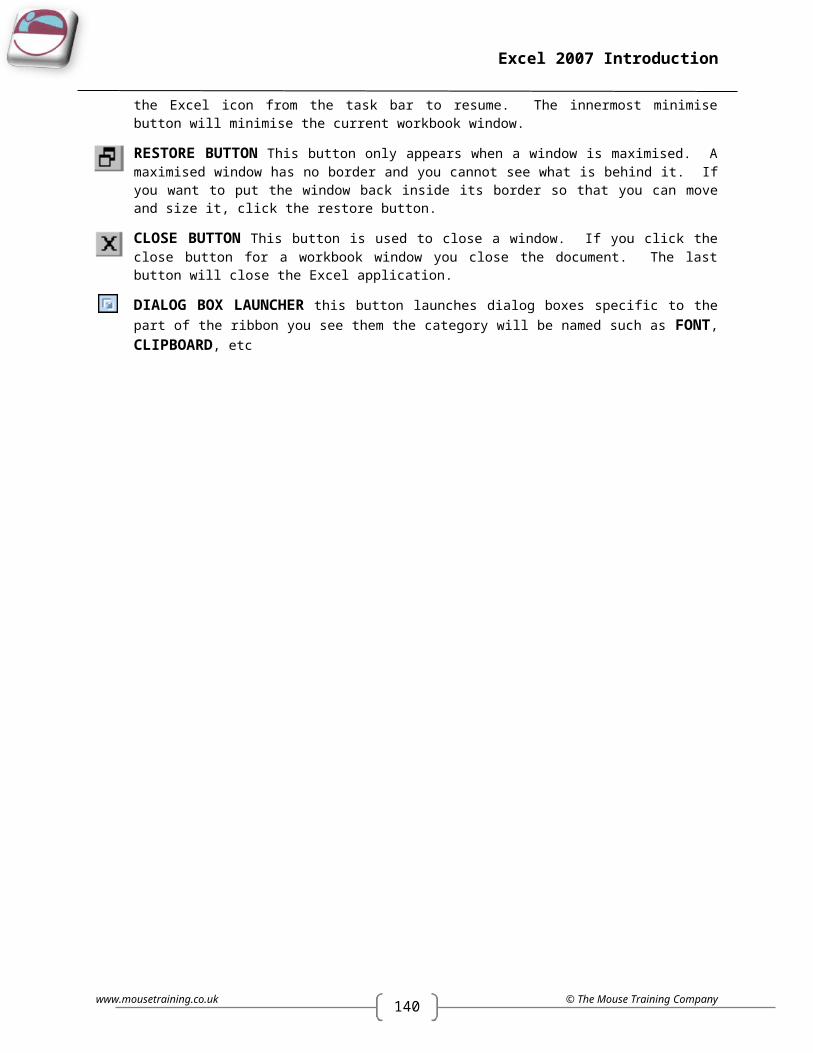
RESTORE BUTTON This button only appears when a window is maximised. A maximised window has no border and you cannot see what is behind it. If you want to put the window back inside its border so that you can move and size it, click the restore button.
CLOSE BUTTON This button is used to close a window. If you click the close button for a workbook window you close the document. The last button will close the Excel application.
DIALOG BOX LAUNCHER this button launches dialog boxes specific to the part of the ribbon you see them the category will be named such as FONT, CLIPBOARD, etc
www.mousetraining.co.uk © The Mouse Training Company

139
Excel 2007 Introduction
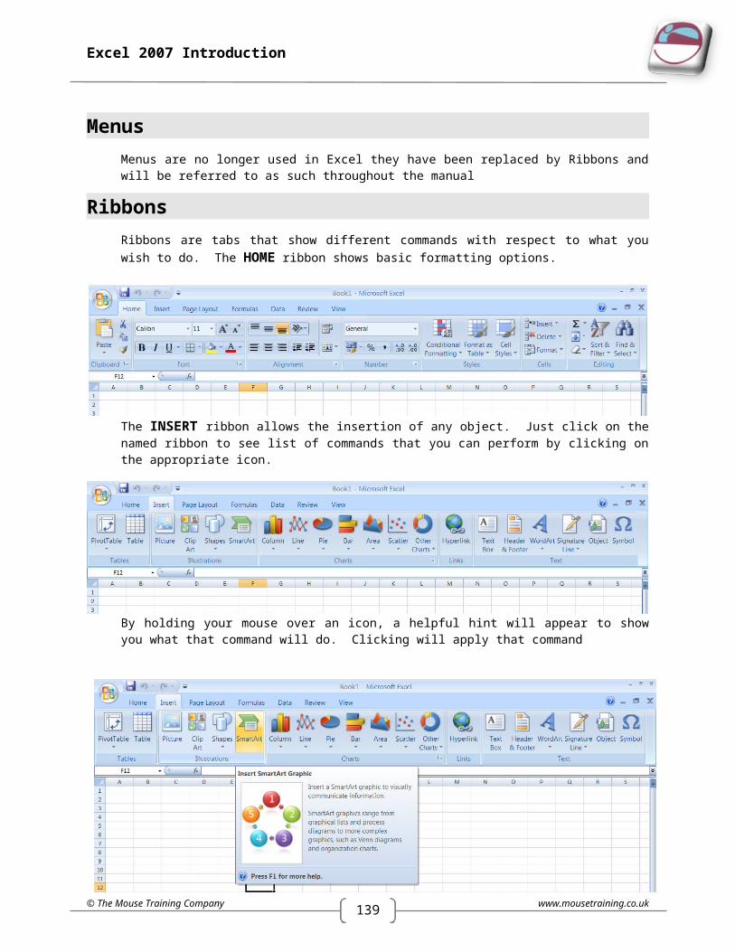
MenusMenus are no longer used in Excel they have been replaced by Ribbons and will be referred to as such throughout the manual
RibbonsRibbons are tabs that show different commands with respect to what you wish to do. The HOME ribbon shows basic formatting options.
The INSERT ribbon allows the insertion of any object. Just click on the named ribbon to see list of commands that you can perform by clicking on the appropriate icon.
By holding your mouse over an icon, a helpful hint will appear to show you what that command will do. Clicking will apply that command
© The Mouse Training Company www.mousetraining.co.uk

140
Excel 2007 Introduction
Any Icon on the ribbon with a down arrow offers other options and sometimes a dialog box.
E.G. choosing a column chart will offer a number of varieties of column charts to insert. Clicking right at the bottom where it offers all chart types will bring up a dialog box to insert any chart type
Dialog BoxTo open a dialog box use dialog box launcher when the dialog box is open, make a choice from the various options and click OK at the bottom of the dialog box. If you wish to change your mind and close the dialog box without making a choice then click on CANCEL. The dialog box will close without any choice being applied. If you would like help while the dialog box is open then click on the “? “ in the top right hand corner this will bring up a help window that will display the relevant topics.
www.mousetraining.co.uk © The Mouse Training Company

139
Excel 2007 Introduction
Look at a group type on the ribbon such as FONT and in the bottom right hand corner of that group you may see a small box with an arrow, clicking this is another method to call up a dialog box, this time, directly from the ribbon. Many dialog boxes may be more familiar if you have used EXCEL before.
Office ButtonThe OFFICE BUTTON is the start of excel and has many important commands and option. Such as excel settings, opening, saving, printing and closing files. This will be explored further later in the manual.
ToolbarsThere are only two toolbars within the new version of Office 2007 there is the QUICK ACCESS TOOLBAR seen here next to the OFFICE BUTTON, and there is the MINI TOOLBAR
Quick Access Toolbar
By default there are only three buttons on the QUICK ACCESS TOOLBAR but these can be edited and other regularly used buttons can be placed there. Using the drop down menu nest to the QUICK ACCESS TOOLBAR will allow the customisation of this toolbar adding your most often used commands.
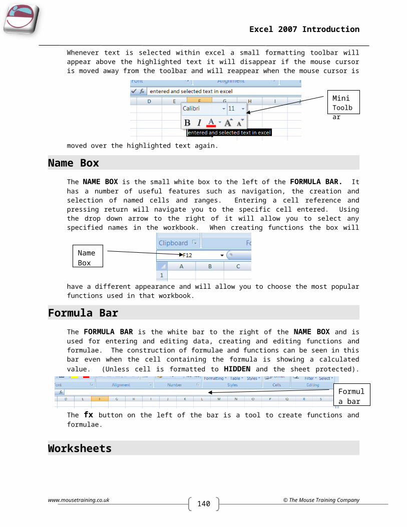
Mini ToolbarWhenever text is selected within excel a small formatting toolbar will appear above the highlighted text it will disappear if the mouse cursor is moved away from the toolbar and will reappear when the mouse cursor is moved over the highlighted text again.
Name Box
© The Mouse Training Company www.mousetraining.co.uk
Office Button Quick
Access Toolbar
Customising menu for toolbar
Mini Toolbar
140
Excel 2007 Introduction
The NAME BOX is the small white box to the left of the FORMULA BAR. It has a number of useful features such as navigation, the creation and selection of named cells and ranges. Entering a cell reference and pressing return will navigate you to the specific cell entered. Using the drop down arrow to the right of it will allow you to select any specified names in the workbook. When creating functions the box will have a different appearance and will allow you to choose the most popular functions used in that workbook.
Formula BarThe FORMULA BAR is the white bar to the right of the NAME BOX and is used for entering and editing data, creating and editing functions and formulae. The construction of formulae and functions can be seen in this bar even when the cell containing the formula is showing a calculated value. (Unless cell is formatted to HIDDEN and the sheet protected). The fx button on the left of the bar is a tool to create functions and formulae.
WorksheetsYou use worksheets to list and analyse data. You can enter and edit data on several worksheets simultaneously and perform calculations based on data from multiple worksheets. When you create a chart, you can place the chart on the worksheet with its related data or on a separate chart sheet. The names of the worksheets appear on tabs at the bottom of the workbook window. The name of the active sheet is bold.
Status BarThe Status bar, across the bottom of the screen, displays different information at different times. To the left is an indicator, which will display Ready, Edit etc. depending on the mode in which the user is currently working. If menus are being accessed, this area will usually give details on the currently highlighted menu option. If you are in the middle of a task – copying data for example – this area will often display messages and prompts instructing you on what to do next.
To the right of the Status bar, keyboard status indicators reveal whether the Num Lock etc. are switched on.
Task Pane
www.mousetraining.co.uk © The Mouse Training Company
Name Box
Formula bar
139
Excel 2007 Introduction
A task pane is a window that collects commonly used actions in one place. The task pane enables you to quickly create or modify a file, perform a search, or view the clipboard.
It is a Web-style area that you can either, dock along the right or left edge of the window or float anywhere on the screen. It displays information, commands and controls for choosing options. Like links on a Web page, the commands on a task pane are highlighted in blue text, they are underlined when you move the mouse pointer over them, and you run them with a single click.
A task pane is displayed automatically when you perform certain tasks, for example when you choose INSERT, CLIPART Ribbons to insert a picture
Smart TagsSmart Tags, first introduced in Microsoft Office XP, make it easier for you to complete some of the more common tasks and provide you with control over automatic features.
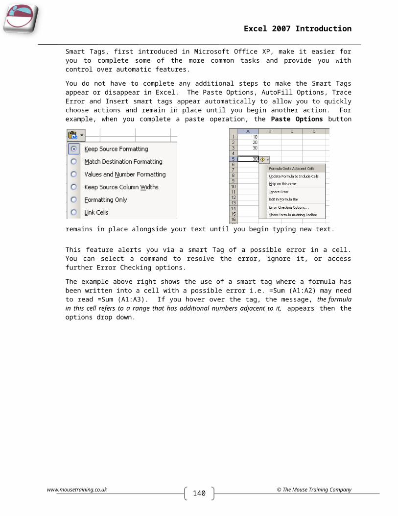
You do not have to complete any additional steps to make the Smart Tags appear or disappear in Excel. The Paste Options, AutoFill Options, Trace Error and Insert smart tags appear automatically to allow you to quickly choose actions and remain in place until you begin another action. For example, when you complete a paste operation, the Paste Options button remains in place alongside your text until you begin typing new text.
This feature alerts you via a smart Tag of a possible error in a cell. You can select a command to resolve the error, ignore it, or access further Error Checking options.
The example above right shows the use of a smart tag where a formula has been written into a cell with a possible error i.e. =Sum (A1:A2) may need to read =Sum (A1:A3). If you hover over the tag, the message, the formula in this cell refers to a range that has additional numbers adjacent to it, appears then the options drop down.
© The Mouse Training Company www.mousetraining.co.uk

140
Excel 2007 Introduction
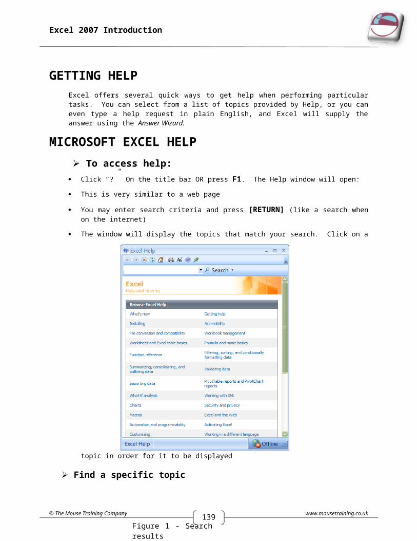
GETTING HELPExcel offers several quick ways to get help when performing particular tasks. You can select from a list of topics provided by Help, or you can even type a help request in plain English, and Excel will supply the answer using the Answer Wizard.
MICROSOFT EXCEL HELP To access help:
Click “?” On the title bar OR press F1. The Help window will open:
This is very similar to a web page
You may enter search criteria and press [RETURN] (like a search when on the internet)
The window will display the topics that match your search. Click on a topic in order for it to be
displayed
Find a specific topic The contents page allows you to select from a list of topic headings. Like search results on the internet
these are HYPERLINKS to help files.
You may need to be online to access some of the help links. The search will be more extensive if you are online as it will search online help files from Microsoft.
www.mousetraining.co.uk © The Mouse Training Company
Figure 1 - Search results

139
Excel 2007 Introduction
SECTION 2 MOVE AROUND AND ENTER INFORMATION
MOVING
Moving Around WorkbookWith such a large working area available, you need to be aware of some of the techniques used for moving around the workbook. It is possible to move using either the keyboard or the mouse.
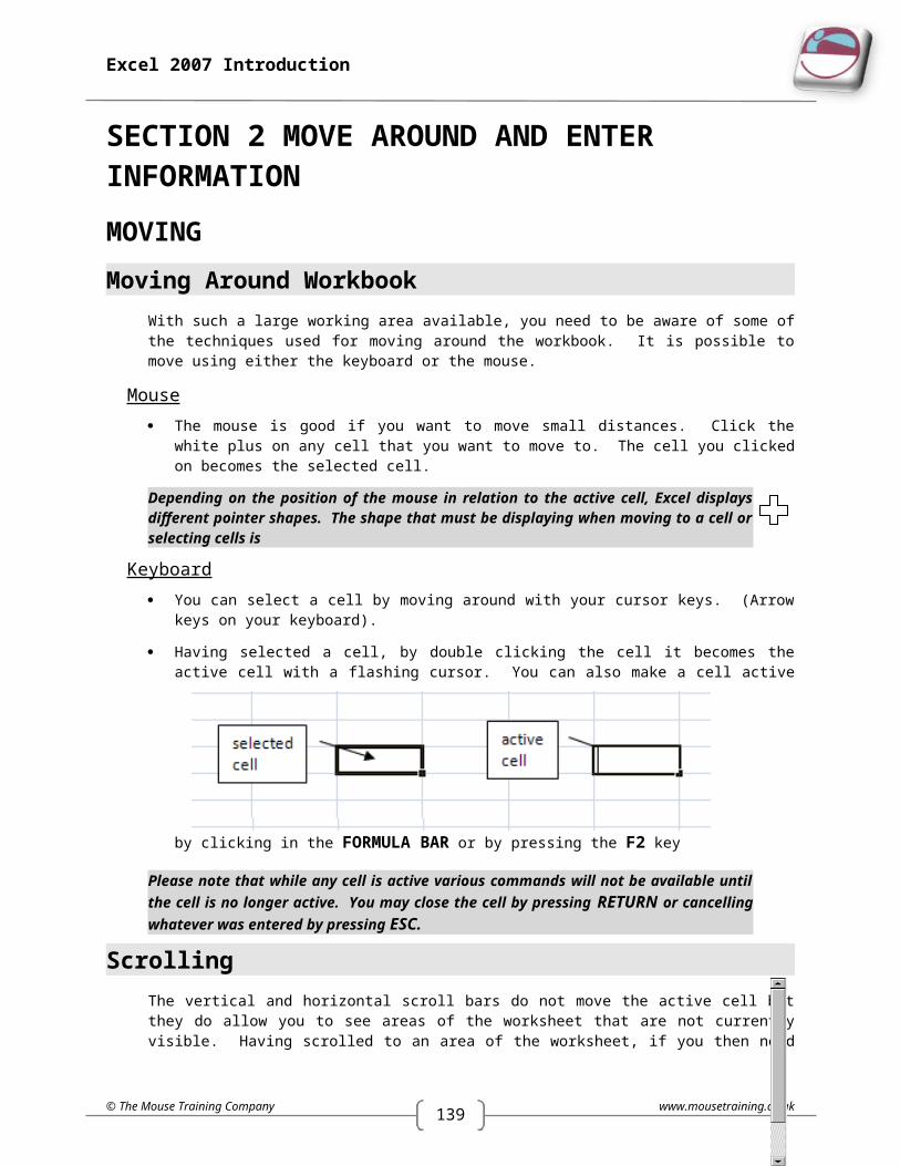
Mouse The mouse is good if you want to move small distances. Click the white plus on any cell that you want
to move to. The cell you clicked on becomes the selected cell.
Depending on the position of the mouse in relation to the active cell, Excel displays different pointer shapes. The shape that must be displaying when moving to a cell or selecting cells is
Keyboard You can select a cell by moving around with your cursor keys. (Arrow keys on your keyboard).
Having selected a cell, by double clicking the cell it becomes the active cell with a flashing cursor. You can also make a cell active by clicking in the FORMULA BAR or by pressing the F2 key
Please note that while any cell is active various commands will not be available until the cell is no longer active. You may close the cell by pressing RETURN or cancelling whatever was entered by pressing ESC.
ScrollingThe vertical and horizontal scroll bars do not move the active cell but they do allow you to see areas of the worksheet that are not currently visible. Having scrolled to an area of the worksheet, if you then need to move the active cell into that region, click the mouse onto a cell of your choice.
To use the scroll bars: Click on the scroll arrows up/down or left/right.
Drag the scroll box until the relevant cell becomes visible.
The size of a scroll box indicates the proportional amount of the used area of the sheet that is visible in the window. The position of a scroll box indicates the relative location of the visible area within the worksheet.
© The Mouse Training Company www.mousetraining.co.uk
140
Excel 2007 Introduction
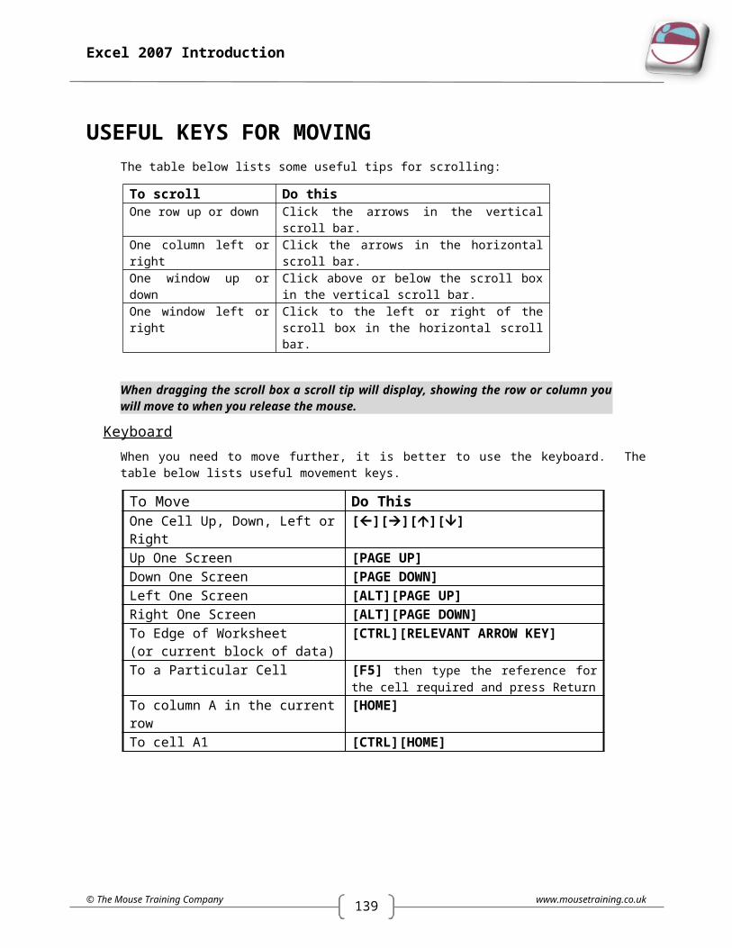
USEFUL KEYS FOR MOVINGThe table below lists some useful tips for scrolling:
To scroll Do thisOne row up or down Click the arrows in the vertical scroll bar.One column left or right Click the arrows in the horizontal scroll bar.One window up or down Click above or below the scroll box in the vertical
scroll bar.One window left or right Click to the left or right of the scroll box in the
horizontal scroll bar.
When dragging the scroll box a scroll tip will display, showing the row or column you will move to when you release the mouse.
KeyboardWhen you need to move further, it is better to use the keyboard. The table below lists useful movement keys.
To Move Do ThisOne Cell Up, Down, Left or Right [][][][]Up One Screen [PAGE UP]Down One Screen [PAGE DOWN]Left One Screen [ALT][PAGE UP]Right One Screen [ALT][PAGE DOWN]To Edge of Worksheet(or current block of data)
[CTRL][RELEVANT ARROW KEY]
To a Particular Cell [F5] then type the reference for the cell required and press Return
To column A in the current row [HOME]To cell A1 [CTRL][HOME]
www.mousetraining.co.uk © The Mouse Training Company

139
Excel 2007 Introduction
WORKBOOK SHEETS
To move between sheetsEach new workbook contains worksheets, named Sheet 1 to Sheet 3. The sheet name appears on a tab at the bottom of the workbook window.
Mouse You may click on any sheet tab to go to that sheet
Keyboard
Press [CTRL][PAGE DOWN] to move to the next sheet, or [CTRL][PAGE UP] to move to the previous sheet.
If the sheet required is not in view, use the tab scrolling buttons to display the sheet.
The last tab is to create a new worksheet, be careful or any new sheets may need to be deleted
Moving Around Sheet
To move to a specific cell:Go To
You can use [F5] to tell Excel to move to a specific cell. [F5] is the Microsoft Office Go To key. When you press [F5] in Excel a dialog box is displayed where you can type in a cell reference.
Keyboard
Press [F5] on the keyboard. The following dialog box will appear.
Type the cell reference that you want to move to in the REFERENCE box and press [RETURN].
You can use [F5] to move to a cell in a different sheet. E.G. To go to Sheet7 cell A1 you can press [F5] and then type Sheet7!A1. (The exclamation mark tells excel that the text immediately before it, is a sheet name. The sheet name must exist in the workbook)
Excel keeps a log of the cells you have visited using the 'Go to' key, and lists them in the 'GO TO' list area of the dialog. You can go back to a previously visited cell by pressing [F5] and double-clicking on the cell reference you want from the list.
Named ranges are also listed in the GO TO list if they have been set up.
DATA ENTRY
© The Mouse Training Company www.mousetraining.co.uk
Sheet tabs
Sheet Tab scrolling buttons
New worksheet tab
140
Excel 2007 Introduction
Enter Text And NumbersThere are various aspects to note and be aware of, both in terms of entering data, and also to do with the nature of the data being entered. You can enter data into a cell by positioning the cursor in the cell and typing the information. The maximum number of characters that a cell can contain is 32,000.
Excel recognises text and numeric entries and initially displays them with different alignments – left for text and right for numbers. You can override these with other formats if required.
To enter information:Mouse
Move to the cell where you want the entry and type a word (for example NAME in cell A1). The text will appear in the Formula bar as well as in the current cell. The cursor will be visible as a flashing insertion point in the formula bar.
Click on the green tick mark on the formula bar to confirm the entry.
OR
Keyboard
Press [RETURN] to confirm the entry.
Until you confirm an entry, Excel remains in "Enter" mode, and the cell is active (see Status bar). Excel will return to the "Ready" mode, and the text will appear in the cell.
When you press [RETURN] to confirm an entry, Excel will by default move the selected cell down to the cell below. You can disable this setting or choose to move the selected cell in a different direction using the EXCEL OPTIONS dialog box (OFFICE BUTTON). See the Customisation section for more information.
Cancelling And Editing Data EntriesYou may find that you have typed an entry into the wrong cell. Provided you have not confirmed the entry by pressing [RETURN] or clicking the green tick from the formula bar, you can abandon it.
To abandon or cancel an entry:Mouse
Click the red cross from the Formula Bar.
OR
Keyboard
Press [ESC] to cancel entry
When you have confirmed an entry, while the cell is still selected, the current cell reference will be displayed in the Name box and the cell contents are displayed in the Formula bar. Text information, as opposed to numeric information, will initially appear left aligned within the cell. If you enter text which is longer than the column width, the display on the worksheet will seem to overlap into the next cell to the right (if that cell is empty).
To edit an unconfirmed entry
www.mousetraining.co.uk © The Mouse Training Company
139
Excel 2007 Introduction
Occasionally, you may make a typing error prior to confirming an entry. You cannot use the arrow keys to move backward you MUST use the formula bar at that point using the arrow keys merely confirms the entry and moves the focus of the selected cell.
To edit a confirmed entry Double click on the cell containing the data to be edited
OR
Press [f2] key
OR
Edit directly in formula bar
Using any of these methods above will allow change the cell to an active cell and allow you to use the cursor keys [][]to move around the data you wish to edit. Use [BACKSPACE] to delete characters behind the cursor or [DELETE] to delete characters in front of the cursor within the data or you may add information to the entry before confirming it.
Enter DatesIt is possible to enter dates into Excel and have them accepted and displayed as such provided you use a recognised format. Excel 2003 will allow entry of dates from 1900 onward.
Recognised formats for datesUse a forward slash (/) as the day/month/year separator: 01/01/01
Use a dash (hyphen) as the day-month-year separator: 1-1-01
Do not use full stops as a date separator as excel will read this as text and the value will not be entered as a true date
Dates entered in excel appear as dates but are actually numbers formatted to appear as dates this allows calculation with them so it is important to enter them correctly. A date once entered correctly will ALWAYS have a four digit year in the formula bar however that date may appear in the cell. Dates start at the number 1 which represents the date 1-1-1900. Dates being numbers align to the right. Any date entered before that date will not be recognised as a true date to excel but will be seen as text and therefore align to the left as with all text.
If you omit the year from a date, Excel will assume the current year. You will not see the year in the cell but if you look at the cell contents on the Formula bar, you will see that Excel has added it.
With some recognised date styles, Excel will automatically format the date to display in a certain way. You can choose how your dates are displayed by formatting them yourself (see the section on formats for more information).
Some entries are recognised by Excel and are formatted automatically. Dates are one such entry (as described above), percentages are another. When you delete data from such cells and replace it with other entries, you may find that you get surprising results. This is because although you cleared the data from the cells, the formats still remain and are causing the new data that you typed to display in a certain way. For more information on clearing cell data, see the clearing cells later in this section.
Autocomplete
© The Mouse Training Company www.mousetraining.co.uk

140
Excel 2007 Introduction
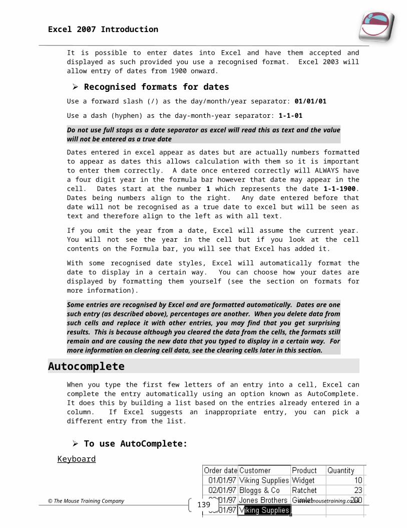
When you type the first few letters of an entry into a cell, Excel can complete the entry automatically using an option known as AutoComplete. It does this by building a list based on the entries already entered in a column. If Excel suggests an inappropriate entry, you can pick a different entry from the list.
To use AutoComplete:Keyboard
Position yourself over the next blank cell in a column.
Begin typing the entry – Excel will try to match what you type with other items already entered in the current column and will automatically complete the entry for you.
Press [RETURN] to accept Excel’s proposed entry.
OR
Continue typing to replace Excel’s proposed entry with your own entry. Press [RETURN] to confirm completion.
Pick From ListYou can get AutoComplete to display a list of possible entries built up from previously entered column data and select the one you want without typing anything.
To pick from an AutoComplete list:Mouse
Click the right mouse button in the required cell.
Choose Pick from List.
Choose the entry required.
OR
Keyboard
Use keys to move to required cell then use [ALT] [↓] to show list and then cursor keys to move through list [RETURN] confirms selection
Excel can only AutoComplete column entries if there are no gaps in your data. If you leave a gap, the next cell that you type in, will not AutoComplete, neither will you be able to pick from a list.
You can stop Excel from AutoCompleting column entries by switching the setting off.
To disable AutoCompleteOFFICE BUTTON, ADVANCED, untick the USE AUTOCOMPLETE checkbox.
EDITING
www.mousetraining.co.uk © The Mouse Training Company
139
Excel 2007 Introduction
There are various ways in which you can change or remove data you have entered in cells on the worksheet.
Typing Replaces SelectionThis option is a feature that is standard throughout the Microsoft Office suite. It ensures that if you type when an item is selected, your typing replaces the selected item. This is extremely useful in a number of instances. When you want to change a short cell entry, it might be quicker to make use of this option to overwrite the entry with the new one.
To overwrite a cell entry:Keyboard
Move to the cell you want to change.
Type in the new entry (the former one will disappear as soon as you start typing).
Press [RETURN] to confirm the changed entry.
Use The Mouse To EditPerhaps one character has been omitted, or two characters have been transposed, and only a slight adjustment needs to be made. If this is the case, you can add or change characters using edit mode. You can edit directly in the cell or on the Formula bar.
To edit in cell: Double-click the cell to change – this will access Edit mode (the prompt on the Status bar will say ‘Edit’).
Use the arrow keys to move the cursor to the edit position within the entry and the [DELETE] and [BACKSPACE] keys to remove characters if necessary.
Press [RETURN] to confirm the changes.
To edit in the Formula bar: Move to the cell to change.
Click in the Formula bar where the cell contents appear. This will drop you straight into Edit Mode (see Status bar) and a cursor appears in the Formula bar.
Use the arrow keys to move the cursor to the edit position within the entry and the [DELETE] and [BACKSPACE] keys to remove characters if necessary.
Press [RETURN] to confirm the changes.
© The Mouse Training Company www.mousetraining.co.uk

140
Excel 2007 Introduction
Using The Keyboard You can access edit mode using a function key.
To edit a cell: Select the cell to be edited.
Tap the [F2] function key. Excel will go into Edit mode. A cursor will appear at the end of the active cell.
Use the arrow keys to move the cursor to the edit position within the entry and the [DELETE] and [BACKSPACE] keys to remove characters if necessary.
Press [RETURN] to confirm the changes.
Select InformationWhen you want to issue a command that will affect several cells, you should select those cells first.
When you select a block of cells, Excel shows you which cell is the active cell within that selection by leaving it white, while the rest of the cells are highlighted black. There are a variety of ways you can select different items on the worksheet and these are described below.
To select cells with the mouseWhen you select with the mouse, you need to make sure that the selection pointer is displayed. This is the white plus that appears when the mouse is positioned over the middle of a cell.
To select Do thisA single cell Click the cell, or press the arrow keys to move to the cell.A range of cells Click the first cell of the range, and then drag to the last cell.
All cells on a worksheet Click the Select All button.Nonadjacent cells or cell ranges Select the first cell or range of cells, and then hold down [CTRL] and
select the other cells or ranges.A large range of cells Click the first cell in the range, and then hold down [SHIFT] and click
the last cell in the range. You can scroll to make the last cell visible.An entire row Click the row number.An entire column Click the column letter.Adjacent rows or columns Drag across the row or column headings. Or select the first row or
column; then hold down [SHIFT] and select the last row or column.Nonadjacent rows or columns Select the first row or column, and then hold down [CTRL] and select
the other rows or columns.More or fewer cells than the active selection
Hold down [SHIFT] and click the last cell you want to include in the new selection
www.mousetraining.co.uk © The Mouse Training Company
139
Excel 2007 Introduction
Select cells with the keyboardSometimes, selecting with the keyboard gives you more control over the amount of data you select. The table below lists the more useful keys for selecting:
To select Do thisThe active cell plus one Cell up, down, left or right
[SHIFT][],[SHIFT][],[SHIFT][],[SHIFT][]
To Edge of Worksheet(Or current block of data)
[SHIFT][CTRL][RELEVANT ARROW KEY]
The current region [CTRL][*] (Use the asterisk from the number pad)
Whole Column [CTRL][SPACEBAR]Whole Worksheet [CTRL][A]
MOUSE
You can cancel a selection by moving somewhere else. Click the white plus on any cell outside the selection.
By using one of the arrow or cursor keys [] or [] or [] or [].
Select Multiple SheetsThere are some situations where you need to select more than one worksheet. The active sheet in a workbook can be determined by its white tab where its name appears in bold.
To select adjacent worksheets:Mouse
Click the tab of the first worksheet that you want to include in your selection.
Hold down the [SHIFT] key and click on the tab of the last worksheet that you want included in your selection. All the sheets between the first and the last will be selected. The selected sheet tabs will turn white and the word ‘Group’ will appear on the title bar.
Select Non-Adjacent Sheets
To select non-adjacent worksheets:Mouse
Click the on the first worksheet’s tab that you want to include in your selection.
Hold down the [CTRL] key and click each other worksheet’s tab that you want included in your selection. The selected sheet tabs will turn white and the word ‘[group]’ will appear on the title bar.
You can cancel sheet selection by clicking on a sheet tab that is not included in the current selection. For more information on working with multiple worksheets, see the relevant section later in this manual.
© The Mouse Training Company www.mousetraining.co.uk

140
Excel 2007 Introduction
CLEAR CONTENTS, FORMATS AND COMMENTSIf you want to remove an entry completely from a cell, you need to clear the cell. There are a variety of ways you can do this and the method you choose depends on what you want to remove from the cell. You can remove data from cells using the ribbons or the keyboard. This command would only remove cell data (numbers, text, dates, formulae). If you have formatted the cells, clearing their contents would leave the formats intact so that new data you type in the cleared cells would keep the old data’s formats.
To clear contents:Mouse
Select the cell or cells you want to clear.
Right click on the cell/selection.
Choose Clear contents from the shortcut menu.
OR
Keyboard Move to the cell or select the cells whose contents you
want to clear.
Tap the [DELETE] key.
If you need to be able to choose what gets removed when you clear a cell, you should use the Clear command under the Edit menu.
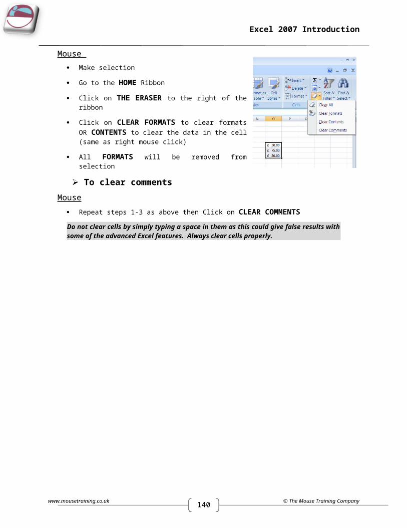
To clear formatsMouse
Make selection
Go to the HOME Ribbon
Click on THE ERASER to the right of the ribbon
Click on CLEAR FORMATS to clear formats OR CONTENTS to clear the data in the cell (same as right mouse click)
All FORMATS will be removed from selection
To clear commentsMouse
Repeat steps 1-3 as above then Click on CLEAR COMMENTS
Do not clear cells by simply typing a space in them as this could give false results with some of the advanced Excel features. Always clear cells properly.
www.mousetraining.co.uk © The Mouse Training Company

139
Excel 2007 Introduction
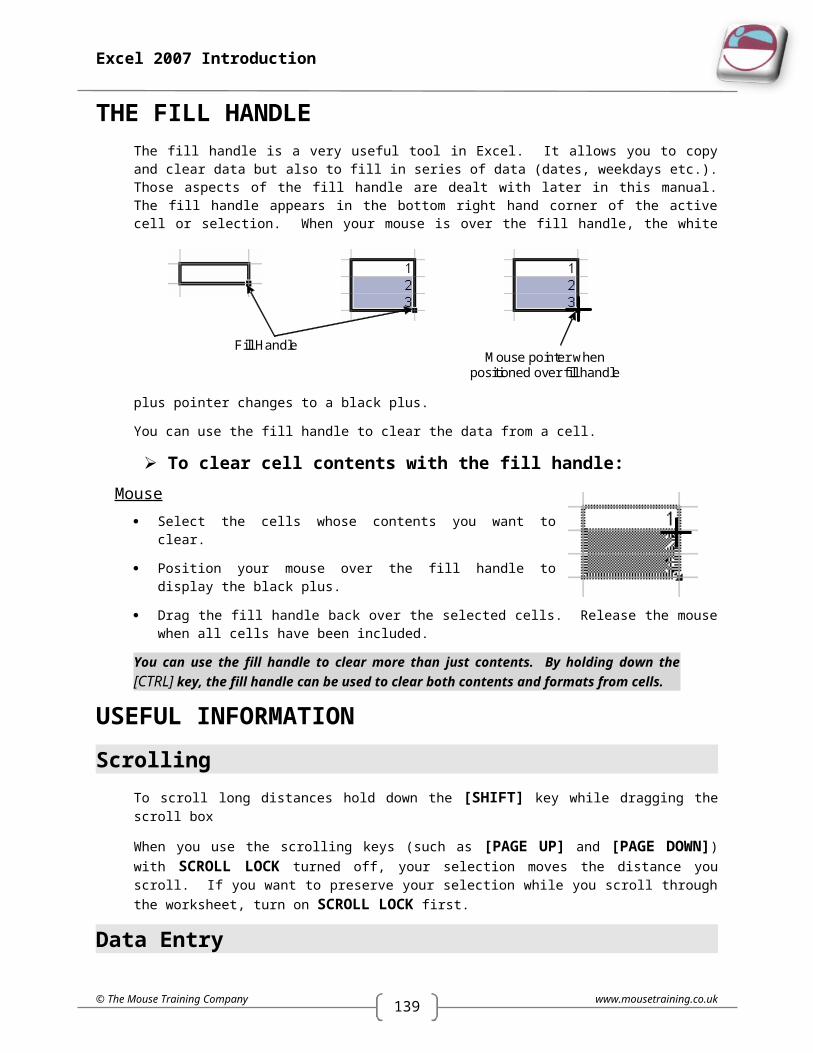
THE FILL HANDLEThe fill handle is a very useful tool in Excel. It allows you to copy and clear data but also to fill in series of data (dates, weekdays etc.). Those aspects of the fill handle are dealt with later in this manual. The fill handle appears in the bottom right hand corner of the active cell or selection. When your mouse is over the fill handle, the white plus pointer changes to a black plus.
You can use the fill handle to clear the data from a cell.
To clear cell contents with the fill handle:Mouse
Select the cells whose contents you want to clear.
Position your mouse over the fill handle to display the black plus.
Drag the fill handle back over the selected cells. Release the mouse when all cells have been included.
You can use the fill handle to clear more than just contents. By holding down the [CTRL] key, the fill handle can be used to clear both contents and formats from cells.
USEFUL INFORMATION
ScrollingTo scroll long distances hold down the [SHIFT] key while dragging the scroll box
When you use the scrolling keys (such as [PAGE UP] and [PAGE DOWN]) with SCROLL LOCK turned off, your selection moves the distance you scroll. If you want to preserve your selection while you scroll through the worksheet, turn on SCROLL LOCK first.
Data EntryYou can enter the current date into a cell by pressing [CTRL][;].
If you want to break a line within a cell, press [ALT][RETURN].
© The Mouse Training Company www.mousetraining.co.uk
Fill Handle Mouse pointer when
positioned over fill handle
140
Excel 2007 Introduction
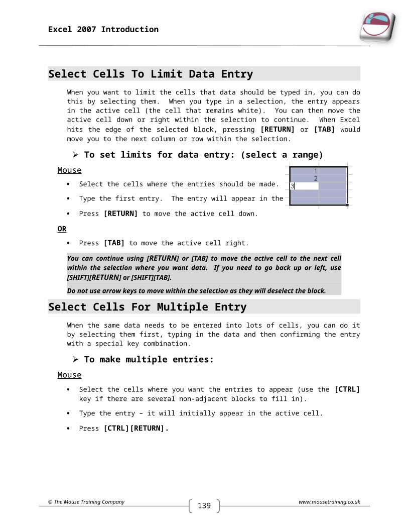
Select Cells To Limit Data EntryWhen you want to limit the cells that data should be typed in, you can do this by selecting them. When you type in a selection, the entry appears in the active cell (the cell that remains white). You can then move the active cell down or right within the selection to continue. When Excel hits the edge of the selected block, pressing [RETURN] or [TAB] would move you to the next column or row within the selection.
To set limits for data entry: (select a range)Mouse
Select the cells where the entries should be made.
Type the first entry. The entry will appear in the active cell.
Press [RETURN] to move the active cell down.
OR
Press [TAB] to move the active cell right.
You can continue using [RETURN] or [TAB] to move the active cell to the next cell within the selection where you want data. If you need to go back up or left, use [SHIFT][ RETURN] or [SHIFT][TAB].
Do not use arrow keys to move within the selection as they will deselect the block.
Select Cells For Multiple EntryWhen the same data needs to be entered into lots of cells, you can do it by selecting them first, typing in the data and then confirming the entry with a special key combination.
To make multiple entries:Mouse
Select the cells where you want the entries to appear (use the [CTRL] key if there are several non-adjacent blocks to fill in).
Type the entry – it will initially appear in the active cell.
Press [CTRL][RETURN].
www.mousetraining.co.uk © The Mouse Training Company
139
Excel 2007 Introduction
SECTION 3 FORMULAE AND FUNCTIONS
FORMULAEIn a spreadsheet application, at a very basic level, values often need to be added, subtracted, multiplied and divided. To allow for the fact that individual values might change, spreadsheet formulae generally refer not to actual values, but to the cells where those values are being held. If values have been entered into A1 and A2, then A1A2 will return an answer which will automatically recalculate if the value of A1 should change. It is this automatic recalculation which makes spreadsheets invaluable.
Excel recognises formulae because they are preceded by an equals sign (=).
When entering basic formulae, the mathematical operators defining the operation to be carried out are as follows:
AdditionSubtraction -Multiplication *Division /Exponentiation ^
You will find all of these mathematical operators ranged across the top and down the right hand side of the numeric keypad.
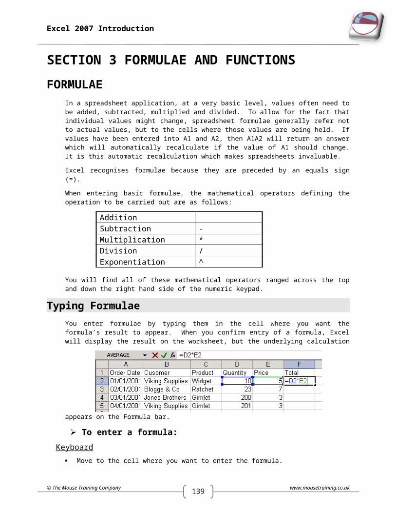
Typing FormulaeYou enter formulae by typing them in the cell where you want the formula’s result to appear. When you confirm entry of a formula, Excel will display the result on the worksheet, but the underlying calculation appears on the Formula bar.
To enter a formula:Keyboard
Move to the cell where you want to enter the formula.
Type an equals sign (=).
Type the formula (e.g. d2*e2).
Press [RETURN] to confirm the entry.
Excel automatically recalculates formulae. If you change one of the cells referenced in your formula, as soon as you press [RETURN] to confirm the changed value, your formula result will update.
© The Mouse Training Company www.mousetraining.co.uk

140
Excel 2007 Introduction
Entering Formulae By PointingIt is possible to enter formulae without actually typing the equals sign (=) or the cell references. Instead, you can make use of a pointing technique to indicate which cells are to be included. As with typing formulae, it is important to start off in the cell where the answer is to be displayed.
Pointing can be quicker and more efficient than typing cell references as it reduces the chances of errors.
To enter a formula using keyboard AND mouse: Position the cursor in the cell where you want the formula.
Type an equals sign (=).
Click the first cell whose reference should be included in your formula. A moving dotted line, known in Excel as a ‘marquee’, will appear around that cell and the cell reference will appear in the formula bar immediately after the equals sign.
OR
Use an arrow key to move there. A moving dotted line, known in Excel as a ‘marquee’, will appear around that cell and the cell reference will appear in the formula bar immediately after the equals sign.
Type in the mathematical symbol you want to use in your calculation, then click on (or move to) the next cell to be included in the formula.
Continue building the formula in this way.
Press [RETURN] to complete the formula.
www.mousetraining.co.uk © The Mouse Training Company
Marquee
139
Excel 2007 Introduction
Errors In FormulaeSometimes you may get surprising results from a formula. This is most often because you have referenced the wrong cell, but it could also be that you have multiplied where you should have added and so on. You can correct formulae using the editing techniques described earlier in this manual.
To edit a formula:Mouse
Double-click on the cell containing the formula. The cell will switch from displaying the result of the formula to the formula itself.
Click the mouse over the part of the formula to change to anchor the cursor there. Type any new characters or use the [BACKSPACE] and [DELETE] keys to remove characters.
Press [RETURN] to confirm the changes.
OR
Move to the cell containing the erroneous formula.
Click on the Formula bar which will show you the formula where you want to make the change.
Type any new characters or use the [BACKSPACE] and [DELETE] keys to remove characters.
Press [RETURN] to confirm the changes.
OR
Keyboard
Press [F2] to access edit mode.
Use the arrow keys to move the cursor to the edit position. Type any new characters or use the [BACKSPACE] and [DELETE] keys to remove characters.
Press [RETURN] to confirm the changes
Filling FormulaeHaving entered an initial formula in the first cell of a column or row, you often find that you want to generate results for the other cells in that column or row. In the example below, you would probably want your formula to work out totals for all the orders.
© The Mouse Training Company www.mousetraining.co.uk

140
Excel 2007 Introduction
There are a variety of ways that you can get Excel to copy a formula so that it generates results for other cells in a column or row.
The Fill Handle And FormulaeThe fill handle has already been described earlier in this manual. It can be used to clear cells but has other uses as well, one of which is filling formulae.
To use the fill handle to copy formulae:Mouse
Move to the cell that has the formula that you want to fill.
Position your mouse pointer over the fill handle. It will change to a black plus.
Drag the black plus down, up, left or right over the cells where you want your copied formula to generate results. You will see an outline around those cells.
Release the mouse when the outline includes all the cells where you want results.
A Smart Tag will be produced. The options it offers are not needed at the moment.
You can also double-click the fill handle to fill down as far as the entries in the adjacent columns
OR
Instead of using the left mouse button to fill down, try using the right mouse button. When released after dragging a menu will appear offering numerous options as to how the data should be filled
www.mousetraining.co.uk © The Mouse Training Company
Fill HandleMouse pointer when
positioned over fill handle

139
Excel 2007 Introduction
Fill Formulae Using KeystrokesYou can fill a column or a row of formulae using the keyboard.
To fill using keystrokes:Keyboard
Select the cell containing the formula to fill and the cells where you want to copy it.
Press [CTRL][D] to fill down.
OR
Press [CTRL][R] to fill right.
There are no keystrokes to fill up or left. Instead, repeat step1 above and then click Edit from the menu bar, choose Fill and select the direction for the fill from the resulting sub-menu.
BODMAS With FormulaeBoDMAS is a mathematical acronym that simply reminds us of the order of operations that mathematics uses to step through more complicated formulae. (Brackets, Division, Multiplication, Addition, Subtraction).
Excel follows these rules to a point please take note of the following table to see the order of preference that excel uses when working out calculations
To change the order of evaluation, enclose in brackets the part of the formula to be calculated first.
1st – Negation (as in –1)2nd % Percent3rd ^ Exponentiation4th * and / Multiplication and division5th and – Addition and subtraction6th & Connects two strings of text (concatenation)7th =
< ><=>=<>
Comparison
Using BODMASE.G. The following formula produces 11 because Excel calculates multiplication before addition. The formula multiplies 2 by 3 and then adds 5 to the result.
Type =52*3 press [RETURN] Result =11
In contrast, if you use parentheses to change the syntax, Excel adds 5 and 2 together and then multiplies the result by 3 to produce 21.
Type =(52)*3 press [RETURN] result = 21
© The Mouse Training Company www.mousetraining.co.uk

140
Excel 2007 Introduction
FUNCTIONS
Sum FunctionHaving mastered how to set up your own custom formulae, you will be able to carry out any calculations you wish. However, some calculations are complicated or involve referring to lots of cells making entry tedious and time consuming. For example, you could construct a formula to generate a total at the bottom of a column (or the end of a row), like this:
=D2D3D4D5
The above formula would work, but if there were 400 cells to total and not just 4, you would get bored with entering the individual cell references and would run out of space (formulae are limited to 1024 characters only).
When formulae become unwieldy or complex, Excel comes to the rescue with its own built-in formulae known as functions.
Functions always follow the same syntax:
The name of the selected function tells Excel what you want to do and the arguments generally tell Excel where the data is that you want to calculate.
Excel has a huge number of functions, not all of them are relevant to everyone. The functions are categorised according to what they do. In this manual, we outline some of the functions that can be used at a general level.
Autosum
using AutosumMouse
Move selected cell to bottom of column or end of row of figures.
Click on the FORMULAS Ribbon, then click on AUTOSUM. From the menu select the SUM function
A ‘marquee’ will appear around the suggested range to sum and a pre-built function will appear in selected cell.
www.mousetraining.co.uk © The Mouse Training Company
=SUM(D2:D5)Equals sign
(Functions are formulae)
Opening and closing brackets
Function argumentsFunction
name

139
Excel 2007 Introduction
If suggested range is correct then press [RETURN]. If not redefine range by selected the figures you wish to include in the function and press [RETURN].
The Shortcut Key For The Sum Function Is [ALT][=]
Other Common FunctionsThe Sum function is very useful, but the AutoSum icon can also be used to for some other common functions: Average (of the selected figures), Count (the number of selected figures), Max (the largest selected figure) and Min (the smallest selected figure).
To use other common functions:Mouse
Select the cell immediately below a column of figures (or to the right of a row of figures) to be totalled.
Click on the drop-down arrow next to the AutoSum icon and select the function that you want to use from the list.
The selected function will automatically appear in the Formula bar and Excel will make a guess at which cells you want to use (you will see a marquee around the cells and their references will be the function arguments).
Press [RETURN] to accept the cells that Excel proposes.
Function LibraryOn the formulas ribbon you will find the function library which is dedicated to functions AUTOSUM functions are just a few of the most regularly used functions.
The functions are broken down in to categories and grouped accordingly to make it easy to access the specific function you desire to use. In many places you will see the MORE FUNCTIONS command which allows access to the whole range of functions available to excel. This brings us to the INSERT FUNCTION utility.
© The Mouse Training Company www.mousetraining.co.uk
140
Excel 2007 Introduction
Insert FunctionIf after looking through all categories you do not find, or find it difficult to locate a specific function then we can use the INSERT FUNCTION facility. Which contains all functions available in excel
To insert functionMouse
Click the cell where you want a result
Go to the FORMULAS ribbon and click on the INSERT FUNCTION icon on the far left
The INSERT FUNCTION dialog box appears
EITHER
Type a description of the function you wish to use in the topmost box and click on go OR select a category from the drop down box
Results will appear in the bottom box then select a specific function with a single click of the mouse
A description will appear underneath the white box and the syntax of how it is constructed
If further explanation is required on a specific function then click on the blue hyperlink in the bottom left corner to get more information.
When the function you want is selected (in this case COUNTA) click OK.
A dialog box appears (below right) with a suggested range for the function. Excel will place the function on the worksheet in the selected cell. You can see the selected function being built on the formula bar. If this is incorrect reselect the range and press [RETURN].
OR
Click the Range selector button. This will collapse the dialog box shown above.
Drag across the cells to replace Excel’s pre selected guess with your own cell references. Click the button marked on the picture below to return to the dialog.
Function Box
www.mousetraining.co.uk © The Mouse Training Company
139
Excel 2007 Introduction
There are some functions that are accessed more than others and for that reason Excel gives you a slightly quicker method for entering them than the Paste function dialog. The Function box, groups the most commonly used functions for quick and easy access.
To enter a function using the Function box:Mouse
Type the equals sign (=) on the formula bar (or directly into your cell). Excel displays the function box to the left of the Formula bar.
Click the drop-down list arrow to the right of the function box to display a list of function names.
Select the function you require by clicking its name from the list.
OR
If your function is not listed, click the More Functions... option to access the Paste function dialog (see above for instructions).
Type FunctionsWhen you get more familiar with functions and start to remember how they are constructed, you can type them rather than selecting them using the previously described methods.
To type a function:Keyboard
Move to the cell where you want the function.
Type an equals sign (=) followed immediately by the function name and an open bracket.
A tool tip appears to indicate the arguments the function needs.
Select (or type) the cells you want the function to act upon using the mouse or arrow keys.
Press [RETURN] to confirm the entry.
As long as your formula only contains one function, you do not need to type the closing bracket. Pressing [RETURN] makes Excel close the bracket automatically.
Function Argument Tool TipsExcel 2007 displays information about function arguments as you build a new formula. The tool tips also provide a quick path to HELP. You click any function or argument name within the tool tip.
© The Mouse Training Company www.mousetraining.co.uk

140
Excel 2007 Introduction
CELL REFERENCESIn functions, you often need to refer to a range of cells. The way Excel displays cell references in functions depends on whether the cells you want the function to act upon are together in a block or in several non-adjacent cells or blocks.
The table below explains how you can use different operators to reference cells:
Operator Description ExampleReference operator: (colon)
Range operator, which produces one reference to all the cells between two references, including the two references
B5:B15
, (comma) Union operator, which combines multiple references into one reference
SUM(B5:B15,D5:D15)
(single space) Intersection operator, which produces one reference to cells common to two references - In this example, cell B7 is common to both ranges
SUM(B5:B15 A7:D7)
Counting And Totalling Cells ConditionallyOccasionally you may need to create a total that only includes certain cells, or count only certain cells in a column or row.
The example above shows a list of orders. There are two headings in bold at the bottom where you need to generate a) the total amount of money spent by Viking Supplies and b) the total number of orders placed by Bloggs & Co.
The only way you could do this is by using functions that have conditions built into them. A condition is simply a test that you can ask Excel to carry out the result of which will determine the result of the function.
www.mousetraining.co.uk © The Mouse Training Company
139
Excel 2007 Introduction
Use Sumif()You can use this function to say to Excel, “Only total the numbers in the Total column where the entry in the Customer column is Viking Supplies”. The syntax of the SUMIF() function is detailed below:
=SUMIF(range,criteria,sum_range)
Range is the range of cells you want to test.
Criteria is the criteria in the form of a number, expression, or text that defines which cells will be added. For example, criteria can be expressed as 32, "32", ">32", "apples".
Sum range these are the actual cells to sum. The cells in sum range are summed only if their corresponding cells in range match the criteria. If sum range is omitted, the cells in range are summed.
=SUMIF(B2:B11, “Viking Supplies”, F2:F11)
With the example above, the SUMIF function that you would use to generate the Viking Supplies Total would look as above.
Using the INSERT FUNCTION tool the dialog would look like this and show any errors in entering the values or ranges
© The Mouse Training Company www.mousetraining.co.uk
140
Excel 2007 Introduction
Use CountifThe COUNTIF function allows you to count those cells that meet a certain condition.
The function syntax is as follows:
=COUNTIF(range,criteria)
Range is the range of cells from which you want to count cells.
Criteria is the criteria in the form of a number, expression, or text that defines which cells will be counted. For example, criteria can be expressed as 32, "32", ">32", "apples".
With our example (shown above), the COUNTIF function that you could use to determine the number of orders placed by Bloggs & Co. would look like this:
=COUNTIF(B2:B11, “Bloggs & Co.”)
www.mousetraining.co.uk © The Mouse Training Company

139
Excel 2007 Introduction
ABSOLUTE AND RELATIVE REFERENCES
Relative ReferencesWhen you fill formulae, you tell Excel to base the formulae it creates on the one you have entered by starting from the cell that contains it.
In the example shown right, the formula being copied says =D2*E2. However, once copied, if you click on any of the copies, Excel will have updated the references to keep the row numbers current (D3*E3, D4*E4 and so on).
This is because Excel, by default, uses relative referencing. When you enter a formula, you enter specific cell references. Behind the scenes, Excel ‘translates’ those references into positions relative to the result cell. So, in our example shown left, Excel would take the formula:
=D2*E2
Translate it as follows:
= [two cells to the left]*[one cell to the left].
It therefore does not matter which row you copy the formula into, Excel will always use “[two cells to the left] multiplied by [one cell to the left]” to generate the result.
Most of the time, this is what you would want, but there are occasions where you need to stop Excel updating cell references when you copy formulae.
Absolute ReferencesThe example below shows a formula being created to work out the amount of discount each order would receive. The order totals are in column F and the discount rate is in B13. The initial formula has therefore been set up as:
=F2*B13
The formula will generate a result for the first order. However, when copied, you will get zeros against the discount amounts for the other orders. This is due to the relative referencing that Excel applies to all formulae by default.
© The Mouse Training Company www.mousetraining.co.uk

140
Excel 2007 Introduction
Having copied the above formula, if you clicked on any formula in the Discount amount column below the first one, you would see that Excel has updated the references (=F3*B14, F4*B15). This is where the problem lies – you want Excel to change the first reference as your formula needs to refer to the different order totals, but the discount rate should remain constant. You need to make that reference absolute.
To make a reference absolute:Keyboard
Move to the cell where you have typed the formula and press [F2] to access Edit mode.
Move the cursor with the arrow keys so that it is next to the reference we want to fix.
Press [F4]. Dollar signs will appear against the column letter and the row number.
Press [RETURN] to confirm the change.
In our example, amending the formula to read:
=F2*$B$13
This would prevent Excel from changing the B13 reference when the formula is copied.
Fill HandleYou can get the fill handle to fill formulas down to the same level as the entries in the previous column by double-clicking on it.
Absolute ReferencesPressing [F4] repeatedly over a reference allows you to toggle between making both the row and column absolute ($A$1), just the column absolute ($A1), just the row (A$1), or nothing absolute (A1).
www.mousetraining.co.uk © The Mouse Training Company

139
Excel 2007 Introduction
SECTION 4 FILE OPERATIONSYou can save any information entered in Excel so that you may call it back at a later stage either to add, edit or print the contents. It’s a good idea to save work frequently as this will minimise the risk of work being lost in the event of a power cut or system fault.
Save FilesExcel gives any new document you create a temporary name – the word ‘Book’ followed by a number. The number increases by one for each new workbook you create in any one work session.
Parts of the SAVE AS dialog box
PREVIOUS FOLDER- As you move through the folder structure in the Files list, this button allows you to go back to the previous folder that you viewed.
UP ONE LEVEL- Click this button to look in the folder that is up one level in the current folder structure.
DELETE- Click this button to delete the selected file or folder.
CREATE NEW FOLDER- Click this button to create a new folder within the current folder.
VIEWS- Click the arrow next to this button to display file and folder view options.
FILE NAME- Type or select a file name for the file that you are saving.
SAVE AS TYPE- In the list, click the file format in which you want to save the file. Most 2007 Microsoft Office system programs can save files in more than one format, so you may need to select the format that you want.
MY PLACES- Click a shortcut on the FAVORITE LINKS bar to save the file to the location represented by the shortcut.
TOOLS- Click TOOLS to display a list of tasks that you can perform. The tools that are available vary depending on the program that you are using.
© The Mouse Training Company www.mousetraining.co.uk

140
Excel 2007 Introduction
SAVE After you determine the location, file name, and format of the file that you are saving, click SAVE to save the file.
CANCEL To go back to the file without saving it, click CANCEL.
Your FAVORITE LINKS bar might be different from what is shown because you can add, remove, or rearrange the shortcuts.
To save a file:Mouse
Click the SAVE button. On the QUICK ACCESS toolbar. If you have not saved the workbook previously, the SAVE AS dialog box will appear asking you for a document name and location.
The first list box marked SAVE IN allows you to determine the drive and folder that you want to save the document in. The area below the SAVE IN list allows you to see which files are stored in the area currently displayed.
To change the location:Mouse
Click the drop-down list arrow to the right of the SAVE IN list box and choose the desired drive or folder.
If you choose a drive, you will see a list of folders within that drive inside the dialog box. If the list is very long, Excel provides you with a horizontal scroll bar to access folders that are not currently visible. Once you can see your folder, you can double-click to open it.
At the bottom of the dialog box are two list boxes, one for the file name and one for the document type. Excel automatically assigns the first few words you typed as the workbook name.
File Types And File NamesExcel in general has always saved files with three letter filetypes such as book1.xls or accounts.xlt the last three letters always being the type of file that it is saved as. In 2007, however, this has now changed and the default filetype for all excel files is now book1.xlsx a four character filetype. This is because the nature of the contents of the file has changed radically and is in no way comparable to earlier versions.
Naming a file:Mouse
Click in the FILE NAME box and drag your mouse over the current file name – this will highlight it.
Type the new name.
Choose from the SAVE AS TYPE box which version of excel you wish to save this file as. (If somebody using a previous version needs to access this file this is essential)
Finally, when the location, name and filetype have been entered, save the workbook by clicking the button marked SAVE. This closes the dialog box. Back in the Excel screen you will notice that the name you allocated to your workbook appears on the TITLE BAR at the top of the screen
www.mousetraining.co.uk © The Mouse Training Company

139
Excel 2007 Introduction
IF you saved this file as an earlier version you will see COMPATIBILITY MODE next to the filename in the TITLE BAR
Workbook names can be up to 255 characters. File names cannot include any of the following characters: forward slash (/), backslash (\), greater than sign (>), less than sign (<), asterisk (*), period (.), question mark (?), quotation mark ("), pipe symbol (|), colon (:), or semicolon (;). You do not need to type the document extension (“.xlsx”) as Excel automatically adds this to all files you save.
Saving Changes To FilesOnce you have allocated a name to a file using the SAVE AS dialog, clicking the SAVE button simply saves any new changes to the name you originally gave. It is worth saving files that you are working on every ten minutes or so. When you click the Save button, the status bar displays a message to say that it is saving and a blue meter which counts up to show how long the save will take.
Keyboard
You can save the current workbook by using the keystroke [CTRL][S]. If the workbook has never been saved before, the SAVE AS dialog will appear, otherwise, [CTRL][S] saves any new changes to the file name that you have already allocated.
Saving As A Different Type Or Different NameIf a file you work with needs to be saved as something else or it needs saving under a different name or maybe another version then we cannot use the SAVE button as this would just save the changes to this file we must call up the SAVE AS dialog again and save the file as something else.
To save as different fileMouse
Click on the OFFICE BUTTON move mouse cursor to SAVE AS
There are various options to choose from with explanations but the top choice will bring the SAVE AS dialog box to the screen again
© The Mouse Training Company www.mousetraining.co.uk

140
Excel 2007 Introduction
Make the necessary changes and click on save
Close Files When you finish working on a file, you can close it down using the following methods:
To close the current file:Mouse
Click on OFFICE BUTTON and choose CLOSE near the bottom of menu.
OR
Click once on the cross (situated on the right-hand side of the screen)
You will see two of the above buttons on-screen – one will close the current file and the other will close the Excel application. To close the current file, use the innermost close button.
If you have changed a file since the last time you saved it, Excel will not let you close that file without prompting you first to save the changes. A dialog box will appear with the option to save the change you have made
www.mousetraining.co.uk © The Mouse Training Company

139
Excel 2007 Introduction
Open Files
To open a file:Mouse
Click on OFFICE BUTTON and choose a recently used file which appears on the right hand side of menu
OR
Click on OFFICE BUTTON and choose OPEN.
The OPEN dialog box will appear
If the file you want is not listed in the window, click the LOOK IN drop-down list box to change to the location of the desired workbook.
To open the file either: Click once on the file name to select it and click the OPEN button.
O R
After locating the file Double-click the file name.
Keyboard
You can also open workbooks using the key combination [CTRL][O]. This will invoke the File Open dialog – follow the steps outlined above to select and open the file that you want.
New Files
To create a new file:Mouse
Click on OFFICE BUTTON and click on NEW The following dialog box will appear
© The Mouse Training Company www.mousetraining.co.uk
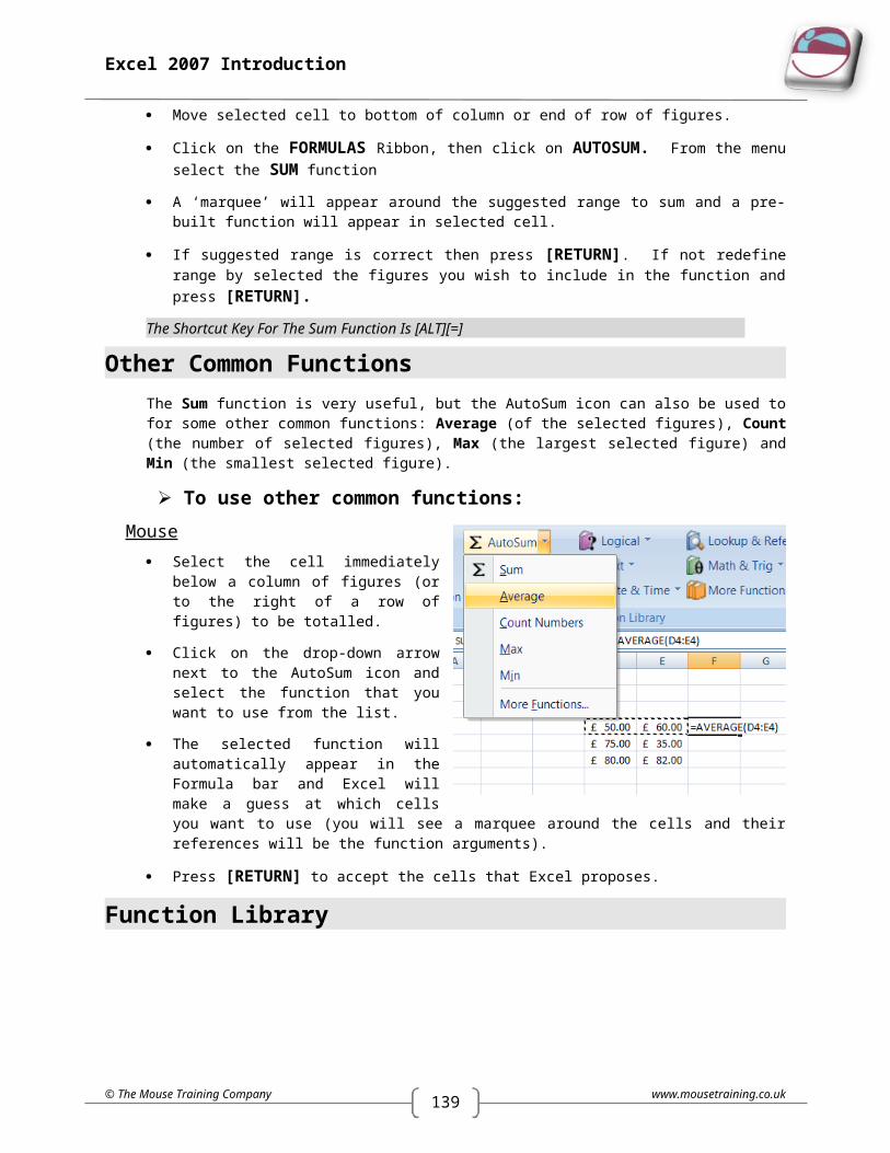
140
Excel 2007 Introduction
On the left are categories of templates. If you are online there are many more choices are available as you can see.
Choosing a category such as BLANK OR RECENT will allow you to create a NEW workbook from any featured in the middle pane only a blank workbook is available at the moment.
A preview of any workbook type is shown on the right.
When you have the correct type of workbook selected even if it is only blank click on CREATE.
OR
Keyboard
[CTRL][N] will create a new blank file.
www.mousetraining.co.uk © The Mouse Training Company
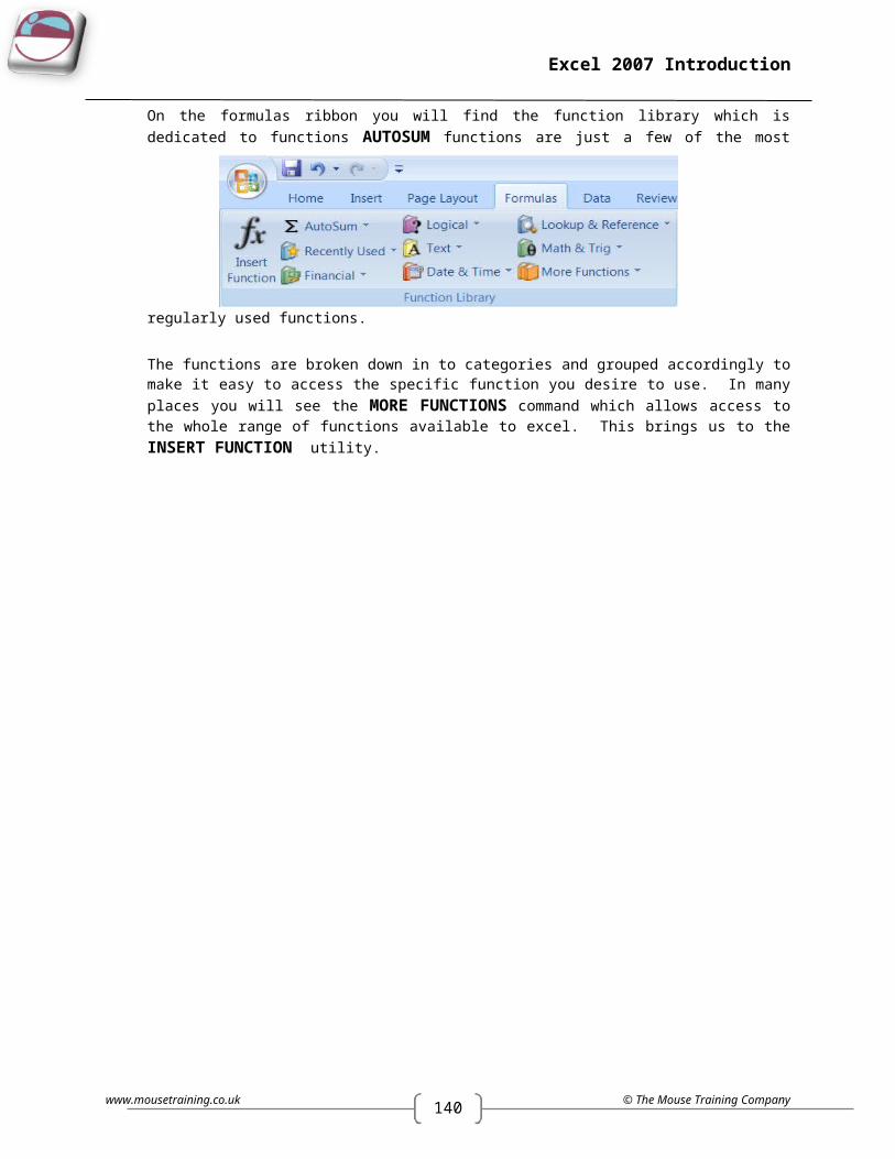
139
Excel 2007 Introduction
Section 5
MOVING AND COPYING DATAHaving entered information in a worksheet, you may decide that you need to reposition it or use cell entries in another worksheet or file that you have created. The good thing about Excel is that once you have entered something once, you can move or copy it anywhere – to other Excel files and even to files that belong to other applications.
All Microsoft products use the same terminology when describing moving and copying items – cut, copy and paste. These terms stem from the times when typesetters would lay out templates by physically cutting an item from its current location, and gluing or pasting it in to the new location.
Moving Items
To move items: Mouse
Select the cells that you want to move.
Click the CUT button on the HOME Ribbon. The selected cells will display a marquee around them and Excel will show a prompt on the Status bar to tell you what to do next.
Move to the cell where you want to place the cells you cut. If you have cut a block of cells, the cell you select before you paste is where you want the top left cell in the cut block to move to.
Click the Paste button from the HOME ribbon
OR
Press [RETURN].
OR
Keyboard Select the cells you want to move.
Press [CTRL][X] to cut the cells out a marquee will appear around the cells, and you will see a prompt on the status bar.
Move to the cell where you want the cut cells to jump to. If you have cut a block of cells, the cell you select before you paste is where you want the top left cell in the cut block to move to.
Press [CTRL][V] to paste the cells into their new location.
© The Mouse Training Company www.mousetraining.co.uk
Status bar prompt
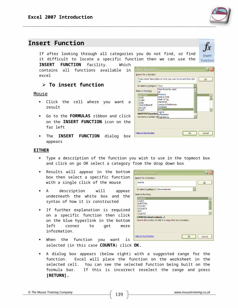
140
Excel 2007 Introduction
Copying Items
To copy items:Mouse
Select the cells that you want to copy.
Click the COPY button on the HOME Ribbon. The selected cells will display a marquee around them and Excel will show a prompt on the Status bar to tell you what to do next.
Move to the cell where you want to place the cells you cut. If you have cut a block of cells, the cell you select before you paste is where you want the top left cell in the cut block to move to.
Click the Paste button from the HOME ribbon the copied cells will appear
OR
Press [RETURN]. The copied cells will appear.
OR
Keyboard Select the cells you want to copy.
Press [CTRL][C] to make a copy. Excel displays a marquee around the copied cells and a prompt on the Status bar.
Move to the cell where you want the copy to go. If you have copied a block of cells, the cell you select before you paste is where you want the top left cell in the copied block to be positioned.
Press [CTRL][V] to paste the copy back in.
OR
Press [RETURN].
ClipboardClicking on the DIALOG BOX LAUNCHER the clipboard will open as a taskpane on the left hand side of the screen
The clipboard holds the last 24 items that have been cut or copied from any of the Microsoft applications and allows you to paste the same item many times in many places including other applications.
www.mousetraining.co.uk © The Mouse Training Company

139
Excel 2007 Introduction
The clipboard is generic to all applications and needs merely to be displayed as it is here. The clipboard can be cleared at any time or single Items deleted
Drag And DropYou can move and copy cells by selecting and dragging them with the mouse. When you do this, you must ensure that you have the correct mouse pointer shape displaying before dragging and dropping.
When you select a cell or a group of cells, Excel outlines them with a heavy border. When the mouse is moved slowly over this border, it will display a white arrow which points up and to the left – and a four arrowed cross in black this is your drag and drop pointer and allows you to move and copy cells with the mouse.
To Move:Mouse
Select the cells you want to move or copy.
Point to the border of the selection.
With the drag and drop pointer displaying, drag the selection to the upper-left cell of the paste area. You’ll see a fuzzy box, the same size as the selected block that will follow your mouse – when you release the mouse the selected cells will jump to their new location.
When you move cells to an area that already has data, Microsoft Excel will ask you to confirm that you wish to replace the existing cell contents with the data you are moving.
To Copy:Mouse
If you want to copy the selection, repeat steps one and two above but before clicking on to it hold down the [CTRL] key on the keyboard, then begin clicking and dragging. You will see a plus sign appear next to the mouse pointer to signal the fact that you are copying rather than moving.
With the fuzzy box positioned where you want the copy, let go of the mouse first and then release the [CTRL] key.
© The Mouse Training Company www.mousetraining.co.uk

140
Excel 2007 Introduction
Shortcut MenusYou can use commands from Excel’s shortcut menus to move and copy items. The shortcut menus appear when you click the right mouse button over a cell or selection.
To move cells:Mouse
Select the cells you want to move.
With the mouse positioned anywhere within the highlighted area, click the right mouse button.
From the resulting shortcut menu, choose CUT. A marquee will appear around the selected cells and the Status bar will display a prompt.
Click the right mouse button over the cell where you want the cut cells to jump to. If you have cut a block of cells, the cell you click before you paste is where you want the top left cell in the cut block to move to.
Choose PASTE from the shortcut menu. The cut cells will jump to their new location.
OR
Press [RETURN]. The cut cells will jump to their new location.
To copy cells:Mouse
Select the cells you want to copy.
With the mouse positioned anywhere within the highlighted area, click the right mouse button.
From the resulting shortcut menu, choose COPY. A marquee will appear around the selected cells and the Status bar will display a prompt.
Click the right mouse button over the cell where you want the cut cells to jump to. If you have cut a block of cells, the cell you click before you paste is where you want the top left cell in the cut block to move to.
Choose PASTE from the shortcut menu. The cut cells will jump to their new location.
OR
Press [RETURN]. The cut cells will jump to their new location.
If you want to insert the cut or copied cells between two rows or columns of existing data, you can use the Insert cut/copied cells option that also appears on the shortcut menu.
www.mousetraining.co.uk © The Mouse Training Company
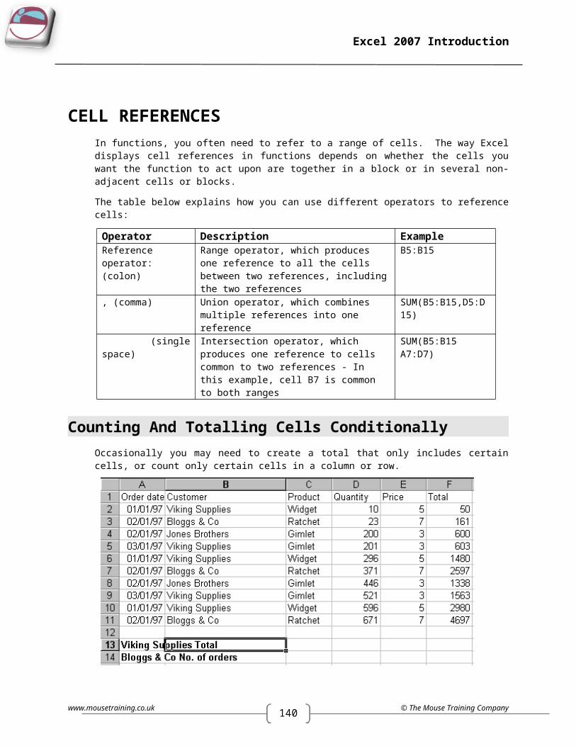
139
Excel 2007 Introduction
Moving And Copying Between FilesYou can use any of the methods described above (even drag and drop) to move and copy items from one workbook to another. When doing this, it is useful to be able to arrange the screen so that you can see the source file (the file containing the items that you want to move or copy) and the destination file (the document where you want to put them) at the same time.
To view open files:Mouse
Open both workbooks using the techniques described in SECTION 4, File Operations.
Click VIEW ribbon, Choose ARRANGE ALL on the ribbon. A dialog box will open to allow you to choose how the files will be arranged. Choose horizontal and the two workbooks will be tiled on screen one above the other, each in its own window.
Use your preferred technique (as described above) to move or copy items from one file to the other.
OR
If you click the SWITCH WINDOWS icon, this will list the files that are currently open to allow you to switch from one file to another. Copying from one file and then switching to paste into another file.
Insert PasteAs already mentioned, Excel will overwrite existing data with cells that you are moving or copying. There are occasions where you want to swap the positions of cells without overwriting what you already have.
In the example above, if you wanted to move the selected cells up two rows so that both “Viking Supplies” orders were next to each other, you would have to use Insert paste to do it, otherwise the existing data (the “Bloggs & Co. order) would be overwritten.
To insert the cells between existing cells:Mouse
Select the cells you want to move or copy.
Point to the border of the selection.
Hold down [SHIFT] (if moving) or [SHIFT][CTRL] (if copying) as you drag. You’ll see a fuzzy line that you can position horizontally (between rows) or vertically (between columns). Release the mouse, then the keyboard. Your cells will jump to their new location.
© The Mouse Training Company www.mousetraining.co.uk
140
Excel 2007 Introduction
Moving And Copying Between WorksheetsWhen you drag cells to areas not currently visibly, Excel will scroll the display down or across allowing you to move or copy the cells to those areas. Sometimes, you may want to drag an item to a different worksheet within the workbook.
To move and copy to another worksheet:Mouse
Select the cells to move or copy and position the mouse over the selection border.
Hold down the [ALT] key as you drag the cells ([ALT][CTRL] if you are copying).
Drag down over the sheet tab that you want to put the cells on and Excel will jump to that sheet. Continue dragging until you are in the location on the selected sheet that you want the cells in. Release the mouse then the keyboard.
Paste SpecialThe Paste Special option gives you the ability to choose what should be pasted into the destination cells. For example, you may want to paste data without its formats, or you might want to convert a formula to a static value – Paste special gives you the choice. You can also use PASTE SPECIAL to add/subtract/divide or multiply the copied cells with the destination cell data.
To use Paste Special:Mouse
Select the cells you want to copy.
Right click anywhere within the highlighted block and choose Copy from the shortcut menu.
Click the right mouse button over the cell where you want the copied data to appear. If you have copied a block of cells, the cell you click before you paste is where you want the top left cell in the copied block to move to.
Choose Paste Special. The following dialog box will appear:
Select an option in the PASTE section of the dialog to choose what will be pasted into the destination cells
Select an option from the OPERATION section of the dialog to choose the mathematical operation you want to perform on the copied data.
Check the SKIP BLANKS box to suppress empty cells being pasted.
Check the TRANSPOSE box to change the arrangement of the copied cells from column to row and vice versa.
www.mousetraining.co.uk © The Mouse Training Company

139
Excel 2007 Introduction
Click OK to close the dialog and paste the data.
© The Mouse Training Company www.mousetraining.co.uk

139
Excel 2007 Introduction
SECTION 6 FORMATTINGHaving produced a spreadsheet, it may be formatted to achieve a more professional and more easily readable layout of data for both screen display and printout. There are several different ways of formatting data in Excel 2007 to produce extremely impressive effects, and many of the tools in the FORMATTING groups on the HOME ribbon are used for the most popular formatting tasks. This section looks at several different approaches to improving the layout of a spreadsheet.
Formatting Groups On Home RibbonThe Formatting groups are together on the HOME ribbon the buttons that create formats most frequently used to enhance worksheet appearance. Not all the formats that you can apply in Excel are contained in the Formatting group icons some can only be accessed via the dialog box which is accessed by the dialog launch button found at the bottom right of a formatting group which is discussed later in this section.
FontBy default, Excel 2007 uses Calibri as its base font and all new worksheets will use this font for data that you enter. However, you can choose different font faces for cells on the worksheet using the Formatting toolbar.
To change the font:Mouse
Select the cells where you want to change the font.
Click the drop-down list arrow to the right of the Font box in the Formatting group on the HOME ribbon.
The fonts are listed alphabetically. Use the vertical scroll bar on the right of the list to move the list items up and down.
Select the desired font by clicking on it. The font face for the selected cells will change to reflect your choice.
OR
Keyboard Select the cells to change.
Press [CTRL][SHIFT][F] to highlight the current font on the formatting toolbar.
Use [ALT] [] to drop down the list of available fonts, use the up and down arrows to move the highlight bar up and down the list and [RETURN] to apply the chosen font to the selected cells.
© The Mouse Training Company www.mousetraining.co.uk
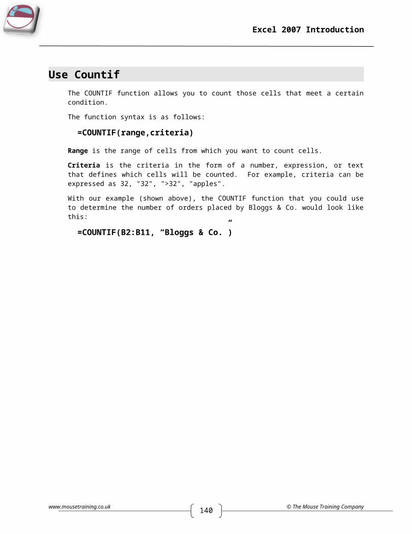
140
Excel 2007 Introduction
Point SizeThis controls the size of the printed characters.
To change the point size :Mouse
Select the cells with the data to change.
Click on the drop-down list arrow to the right of the currently displayed point size.
Pick a new number from the list – the selected cell data will change size accordingly.
OR
Keyboard Select the text to change.
Press [CTRL][SHIFT][P] to highlight the current point size on the formatting toolbar.
Either type the point size that you want to use (your typing will replace the currently selected number) or use [ALT][] to display the list of point sizes and move the highlight bar to the selected size using the up and down arrow keys.
Press [RETURN] to apply the currently highlighted size to the selected cells.
OR
MouseAfter selecting cells you may use your mouse to increase or decrease the size of your font in the selected cells by clicking on the increase or reduce point size buttons in the font group. This will change the size of your font one point at a time
Although Excel displays from 8 to 72 points in the list, you can type your own numbers in and press [RETURN] to apply the format)
Bold, Italic And UnderlineBold, italic and underline can be applied to the selection using buttons on the formatting toolbar or keyboard shortcuts.
Apply bold, italic or underline: Mouse
Select the cells to change.
Click on either the B, I or U buttons on the toolbar. The button will “switch on” and the selected text will display the applied format.
Clicking on the underline drop down arrow will give you the option of having double underline instead of the regular single one. You may still toggle this off by clicking the U again
www.mousetraining.co.uk © The Mouse Training Company
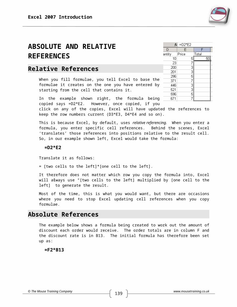
139
Excel 2007 Introduction
OR
Keyboard Select the cells to change.
Press [CTRL][B] to apply bold formatting, [CTRL][I] to apply italic formatting or [CTRL][U] to apply single underline formatting to the selected cell data.
Remove Bold, Italic and Underline:Mouse
Select the cells with the format.
Click the Bold, Italic or underline button to turn the format off.
OR
Keyboard Select the cells with the format.
Press [CTRL][B], [CTRL][I] or [CTRL][U] to switch the format off.
Font ColourThis will change the colour of on-screen information. It will also print the information in the chosen colour if you are connected to a colour printer.
To change font colour:Mouse
Select the cells whose font colour you want to change.
Click the drop-down list arrow displayed on the right-hand side of the button and choose the desired colour.
Themes (see later) show complimentary colours and shades on the theme that you may have chosen for your worksheet (those in figure are default)
There are also standard colours to choose from
If you still cannot find what you want from the default palette there are more colours to choose from. Click more colours to find any colour you desire.
To reset font colour:Mouse
Select the cells you want to reset to the default colour.
Click the drop-down list arrow displayed on the right-hand side of the Font colour button.
The AUTOMATIC option will reset text back to the default colour (normally black).
© The Mouse Training Company www.mousetraining.co.uk
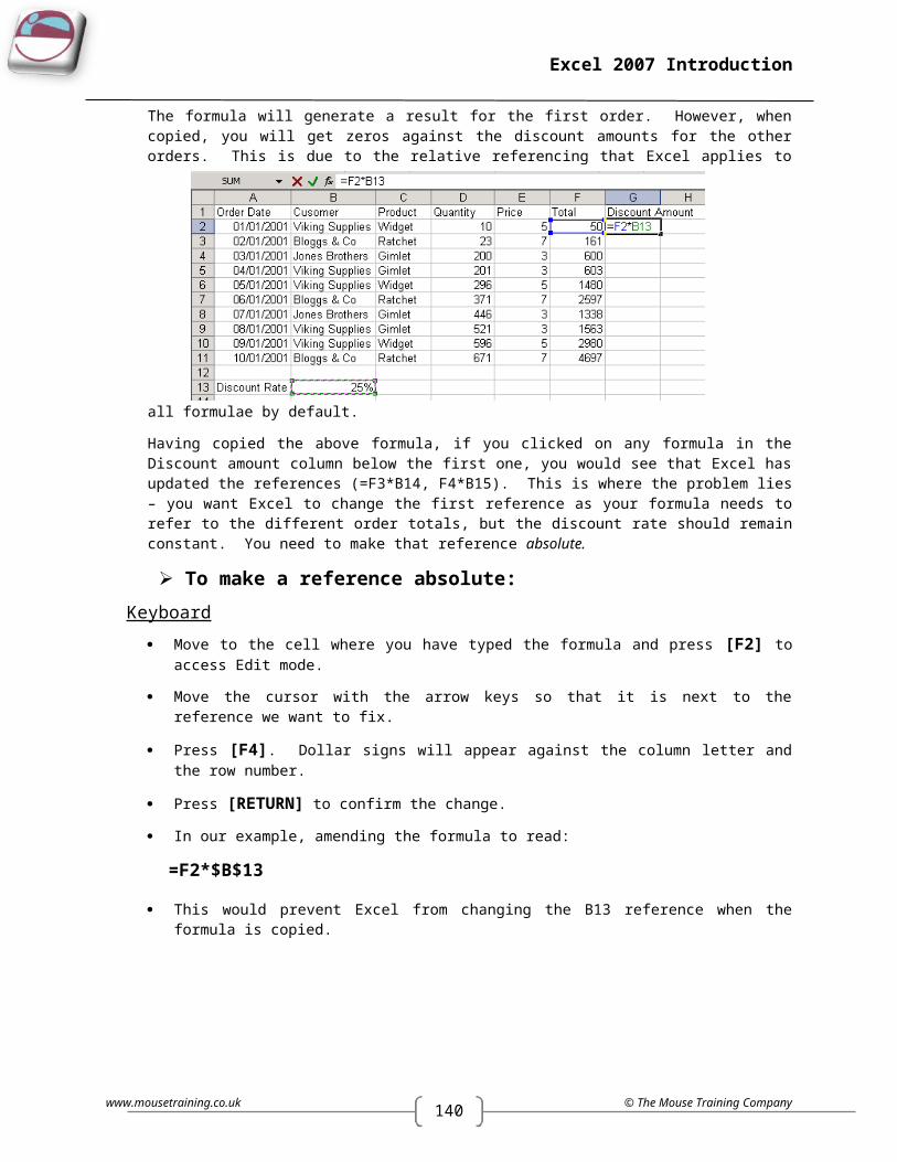
140
Excel 2007 Introduction
Background Fill ColourIf you want to shade the background of cells, use the Fill colour button.
To change fill colour:Mouse
Select the cells whose background colour you want to change.
Click the drop-down list arrow displayed on the right-hand side of the Fill colour button.
The NO FILL option will remove any applied fill colours.
The fill colour palette has the same range of colours and colour options that in the text colour drop down list
BordersWhen you print a worksheet, Excel allows you to choose whether you want all the cell gridlines to print or not. Often, you want to print some but not all of the lines – this is when you need to apply borders. You can then tell Excel not to print the gridlines but your borders will be printed.
To apply borders:Mouse
Select the area you want to border.
Click the drop-down list arrow to the right of the Borders button on the Formatting toolbar.
From the palette, click on the required border option.
If the palette does not have the bordering option that you want to apply, use the Format cells dialog (discussed later in this section) to apply the borders.
To remove borders:Mouse
Select the area with the borders you want to remove.
Click the drop-down list arrow to the right of the Borders button on the Formatting toolbar.
From the palette, click on the first border option.
www.mousetraining.co.uk © The Mouse Training Company

139
Excel 2007 Introduction
AlignmentYou can select from three different cell alignment options in Excel by clicking the relevant button (described below). The buttons determine how data lines up between the left and right edges of the selected cell(s).
To change alignment:Mouse
Select the cell(s) whose alignment you want to change.
Click on the button for the alignment you require (see below).
Click this button to left-align cell data. Left alignment ensures that the left edge of an entry is flush with the left edge of the cell. Left alignment is the default alignment for text entries in cells.
Click this button to centre cell data. This will make each cell entry in the selection position itself in the middle of the cell.
Click this button to right-align cell data. Right alignment ensures that the right edge an entry is flush with the right edge of the cell. Right alignment is the default for numeric cell entries.
Merge CellsIf you want to type a heading across the top of a table of data, it can be quite difficult to line it up in the centre. If the columns in your table are different widths, or the title is a certain length, the chances of you getting it exactly central along the top of the table are practically nil. Luckily Excel has a solution. You can merge the cells across which you want the heading, centring it at the same time.
To merge cells:Mouse
Select the cells you want to merge.
Click the MERGE AND CENTRE button from the Formatting toolbar.
© The Mouse Training Company www.mousetraining.co.uk

140
Excel 2007 Introduction
To Unmerge cellsMouse
Select the cells you want to unmerge
Click the Merge and Centre button again and this will unmerge the cells selected
As you can see from the figure right if you click the drop down arrow to the right of the merge cell button you have options to merge cells with different alignments.
IndentsIndents allow you to control where a cell entry begins inside a cell.
To indent cell data:Mouse
Select the cell(s) where you want an indent.
Click the increase indent button to indent the selected cell data by a standard amount from the left. You can click this button again to increase the amount of indent and so on.
If you need to take the indent back, click the decrease indent button to do this.
Number FormatsInitially, numbers in Excel use a General format. You may find that the results of formulae run to different numbers of decimal places, or you might want to display numbers as monetary values with a currency symbol and two decimal places. There is no need for you to enter the numbers in the way you want them displayed – it is far better to use Excel’s number formatting buttons.
INCREASE AND DECREASE DECIMAL PLACES
You can add and remove decimal places from numeric data using the Increase Decimal and Decrease Decimal buttons. Where you decrease, Excel will round numbers up or down to the nearest unit. However many places that you may increase or decrease the value to excel will still use the entered value to calculate not the value that appears in the cell as this is only an appearance not a true value (check formula bar)
To increase decimals:Mouse
Select the cells with the numbers you want to change.
Click the INCREASE DECIMAL button from the ALIGNMENT group on the HOME ribbon
Keep clicking the INCREASE DECIMAL button until your numbers display the correct number of decimal places.
www.mousetraining.co.uk © The Mouse Training Company

139
Excel 2007 Introduction
To decrease decimals:Mouse
Select the cells with the numbers you want to change.
Click the DECREASE DECIMAL button from the ALIGNMENT group on the HOME ribbon
Keep clicking the Decrease Decimal button until your numbers display the correct number of decimal places.
COMMA STYLE
Comma style sets all the selected numbers to 2 decimal places and puts commas between different thousand multiples.
E.G. 100000 would become 100,000.00 when comma style is applied to it.
To apply comma style:Mouse
Select the cells with the numeric data you want to format.
Click the Comma Style button from the Number group on the HOME ribbon
CURRENCY
Applying this style will add a £ sign and two decimal places (pence) to the selected numbers.
To apply currency style:Mouse
Select the cells with the numeric data you want to format.
Click the Currency button from the Number group on the HOME ribbon.
Using the drop down arrow to the right of the currency button gives access to the most likely used currency formats in use you can choose from different currency symbols using the FORMAT CELLS dialog discussed later in this section
PERCENT STYLE
Where you have typed decimals on the worksheet, you may want to express those values as percentages. You can do this with the Percent Style format.
E.G. 0.5 would become 50% when you apply Percent Style.
To apply Percent Style:Mouse
Select the cells with the numeric data you want to format.
© The Mouse Training Company www.mousetraining.co.uk
140
Excel 2007 Introduction
Click the Percent Style button from the Formatting toolbar.
The number formats (apart from Increase and Decrease Decimal) are mutually exclusive. Applying Comma Style to cells that already have Currency formats would lose the currency symbol. If you need to return to the default General style for numbers, you can use the Format Cells dialog discussed later in this section.
If you ever see ###### in cells that normally display numbers, it is because the format you have applied is too wide for the column. To show the numbers, either change to a format that fits or widen the column (see later in this section for details on changing column widths).
Advanced FormatsWhen you want to apply formats that Excel does not give you buttons for on the Formatting toolbar, you need to use the Format Cells dialog. This dialog contains all the formatting options (including those accessible via the Formatting toolbar) that you can use within the Excel application.
Format Cells DialogThe Format Cells dialog is divided into tabs, each tab dealing with a format category.
To access the Format Cells dialog:Mouse
Select the cells whose formats you want to change.
Click the DIALOG BOX LAUNCHER. From either the FONT, ALIGNMENT or NUMBER group on the HOME ribbon
OR
Keyboard
Press [CTRL][1]
The dialog box as seen top of next page will appear. Depending on which DIALOG BOX LAUNCHER you clicked will depend on which tab will appear first of the six in the dialog box
Once the dialog is on-screen, you can move between the format categories by clicking on the labelled tabs and change settings on each. Each tab has a Preview window to show you what the effects of your changes will look like should you choose to apply them. When all the formats have been set, click the OK button to close the dialog and apply the new formats.
www.mousetraining.co.uk © The Mouse Training Company
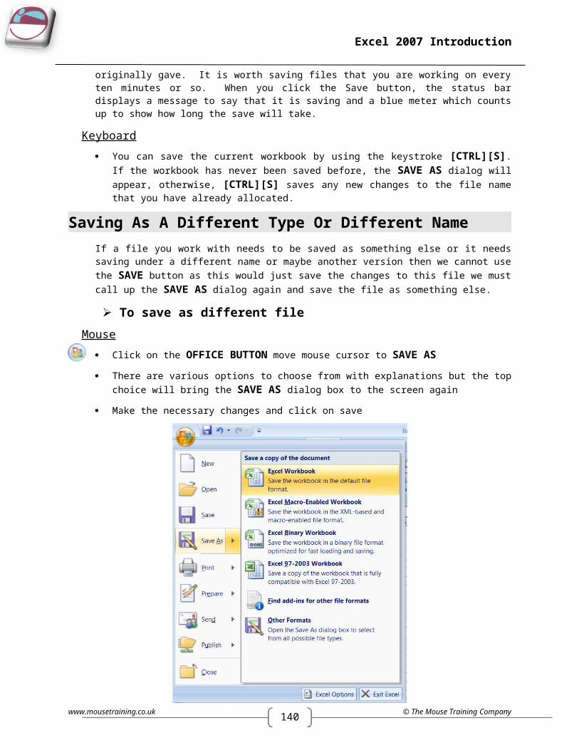
139
Excel 2007 Introduction
FONT TAB
Most of the formats you find on the Font tab of the Format cells dialog can be applied directly from the Formatting Toolbar and need no further discussion. However, there are some extra Effects that can be applied should you need to do so.
To apply effects:Mouse
Select the cells you want to format.
Click the DIALOG BOX LAUNCHER. From either the FONT, ALIGNMENT or NUMBER group on the HOME ribbon
Click the FONT tab.
Check the STRIKETHROUGH, SUPERSCRIPT or SUBSCRIPT boxes (the PREVIEW window will show you what the formatting will look like on sample data).
Click OK to close the dialog and apply the changes.
The Superscript and Subscript options are mutually exclusive.
© The Mouse Training Company www.mousetraining.co.uk

140
Excel 2007 Introduction
ALIGNMENT TAB
The settings on this tab give you lots of options for alignments which are not available on the Formatting toolbar.
HORIZONTAL ALIGNMENT
Most of the formats for horizontal alignment are available on the Formatting toolbar, however there are some extras:
Justify - where you have several lines of data in a cell, you can ensure that the left and right edges of the data are straight.
Fill – use this to repeat the selected cell entries within their cells so that the entire cell from left to right is full.
To change horizontal alignment:Mouse
Select the cells you want to format.
Click the DIALOG BOX LAUNCHER. From either the FONT, ALIGNMENT or NUMBER group on the HOME ribbon
Click the ALIGNMENT tab.
Click the drop-down list arrow to the right of the Horizontal list box.
Choose the alignment by clicking on the required option from the list.
Choose OK to close the dialog and apply the changes.
www.mousetraining.co.uk © The Mouse Training Company

139
Excel 2007 Introduction
VERTICAL ALIGNMENT
Use the options in this list to choose how data lines up between the top and bottom edges of cells.
To change vertical alignment:Mouse
Select the cells you want to format.
Click the DIALOG BOX LAUNCHER. From either the FONT, ALIGNMENT or NUMBER group on the HOME ribbon
Click the ALIGNMENT tab.
Click the drop-down list arrow to the right of the VERTICAL list box.
Choose the alignment by clicking on the required option from the list.
Choose OK to close the dialog and apply the changes.
TEXT CONTROL
The text control options allow you to determine how the size of the data in the selected cells will affect columns and rows.
Wrap text - Where you have an entry that is too wide for the column, you can get Excel to wrap within a cell. Where a single line becomes multiple lines, Excel will automatically adjust the row height.
BEFORE AFTER
Shrink to fit - Reduces the apparent size of font characters so that all data in a selected cell fits within the column. The character size is adjusted automatically if you change the column width. The applied font size is not changed on printouts.
BEFORE AFTER
Merge cells - Makes the selected cells into one cell.
Where there are entries in all the selected cells, when you merge them together, Excel will warn you that it will only keep the entry in the top left cell in your selection.
To change text control settings:Mouse
Select the cells you want to format.
Click the DIALOG BOX LAUNCHER. From either the FONT, ALIGNMENT or NUMBER group on the HOME ribbon
Click the ALIGNMENT tab.
Check the relevant options under the TEXT CONTROL heading to switch on the effect.
Click OK to close the dialog and apply the new formats.
© The Mouse Training Company www.mousetraining.co.uk
Viking Supplies Viking Supplies
Viking Supplies Viking Supplies
140
Excel 2007 Introduction
ORIENTATION
You can display and print data in Excel oriented any way you choose.
BEFORE AFTER
Shown above are some examples of different orientations.
To change orientation:Mouse
Select the cells you want to format.
Click the DIALOG BOX LAUNCHER. From either the FONT, ALIGNMENT or NUMBER group on the HOME ribbon
Click the ALIGNMENT tab.
In the ORIENTATION section, to keep characters horizontal but arrange them one underneath the other, click the picture that corresponds.
OR
Drag the red dot marker up or down to give a degree value of plus or minus 90° from the base position (horizontal).
Click OK to apply the new formats and close the dialog.
www.mousetraining.co.uk © The Mouse Training Company
CustomerCustomer
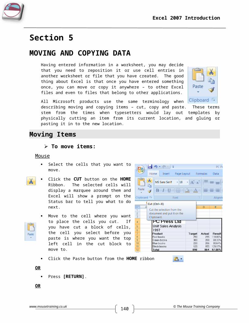
139
Excel 2007 Introduction
PATTERNS TAB
You can use settings on the Patterns tab to not only add background fill colours to cells, but apply patterns to them as well.
To apply patterns to cells:Mouse
Select the cells you want to format.
Click the DIALOG BOX LAUNCHER. From either the FONT, ALIGNMENT or NUMBER group on the HOME ribbon
Click the PATTERNS tab.
Click the drop-down list arrow on the right of the PATTERNS box to display a palette of colours for the pattern.
Choose the pattern that you want (i.e. lines, dots etc). If you want to change what colour the lines/dots etc. that make up your pattern will be, access the palette once again and click a colour.
The colour palette on the left will give the cell a background colour
Click the fill effects button to choose more advanced patterns and colouring. The fill effects dialog will be launched (This will be discussed later. It is a dialog box that is used for filling colours and patterns of many types of objects.)
Choose the more background colours the more colours button a separate dialog box will be launched with an extensive choice of colours
The SAMPLE pane will display what the chosen formats will look like should you choose to apply them. Choose OK to close the dialog and apply your formats.
© The Mouse Training Company www.mousetraining.co.uk

140
Excel 2007 Introduction
BORDERS TAB
You can change border line sty les, colours and directions using the Borders tab.
To apply custom borders:Mouse
Select the cells you want to format.
Click the DIALOG BOX LAUNCHER. From either the FONT, ALIGNMENT or NUMBER group on the HOME ribbon
Click the BORDER tab.
Choose the line style by clicking on the appropriate line from the STYLE palette.
Choose the line colour by clicking on the drop-down arrow to the right of the COLOUR box to access a colour palette. Click the colour you want your border to be.
In the BORDER section, set which edges of your selection need bordering by clicking the button which shows the relevant edge.
OR
If there are multiple edges that need borders, click the preview diagram (where the word “Text” sits) along the edges that you want the borders. Clicking the word “Text” in the preview diagram will give diagonal borders. One click will add a border, another will remove it.
OR
Use the preset buttons to apply a borders see the effects in the preview
Click the OK button to close the dialog and apply your changes.
NUMBERS TAB
www.mousetraining.co.uk © The Mouse Training Company
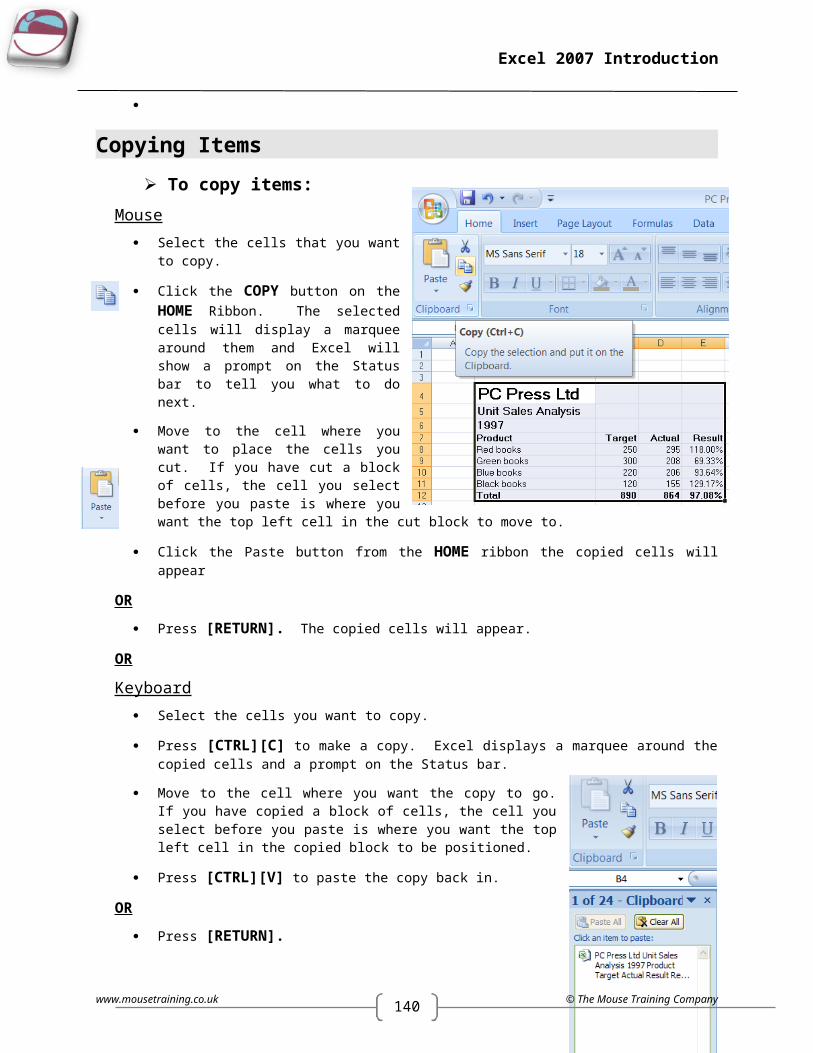
139
Excel 2007 Introduction
The Numbers tab gives you the ability to display data that Excel stores numerically in lots of different ways. The Formatting toolbar gives you buttons for applying only very few of the vast selection of number formats that Excel contains. The options that you see on the tab vary depending on which category of format you select. Generally speaking, Excel will display a sample based on the contents of the active cell and the default option within the category you selected. You can then pick from a list of format codes until the sample is displayed the way you want it.
To apply number formats:Mouse
Select the cells you want to format.
Click the DIALOG BOX LAUNCHER. From either the FONT, ALIGNMENT or NUMBER group on the HOME ribbon
Click the NUMBER tab.
Click the category of formatting your numeric data should use from the CATEGORY list.
Select the relevant options that appear until the SAMPLE data looks the way you want your numbers to look.
Click OK to close the dialog and apply the format.
© The Mouse Training Company www.mousetraining.co.uk
Category
Sample of format
(preview)
Choose settings for format here
The custom category
allows creation of
personalised formats using
codes.

140
Excel 2007 Introduction
Custom Number FormatsThere are occasions when you want numeric data to display in a way that Excel does not have a format for. When this happens, you can create a custom format.
To create a custom number format:Mouse
Select the cells you want to format.
Click the DIALOG BOX LAUNCHER. From either the FONT, ALIGNMENT or NUMBER group on the HOME ribbon
Click the NUMBER tab. Then choose the Custom category (the last option on the Category list). The dialog box will change to show you a list of Type format codes.
Scroll down the Type list until you find a code similar to the one you want to format your data with.
For example, if you wanted to change a date currently displaying as 01/01/2000 to display as “January”, select the format code “mmm-yy” to give you a base to alter – it would initially display your date as “Jan-2000”, but you can change it to what you want.
Click in the Type box and amend the code to give the display you want (watch the sample as you do this). For the example mentioned above, you would type “mmmm”. When you have the correct code, click OK to close the dialog and apply the custom number format.
Custom formats, once created, only exist in the file that they were set up in. If you want to use them in another workbook, you can copy the format across. You can copy formats only using Paste Special (see Section 5 for more information).
www.mousetraining.co.uk © The Mouse Training Company

139
Excel 2007 Introduction
PROTECTION TAB
You can use the settings on this tab to control which cells are accessible when you protect a worksheet. This topic is dealt with in the section “Working with multiple sheets” later in this manual.
FORMATTING COLUMNS AND ROWSExcel has some formats that apply themselves to whole columns and rows. Changing widths and heights, hiding, inserting and deleting rows and columns are all operations that you might want to carry out.
Column WidthYou can alter the width of a single column, or by selecting the columns whose width you want to change, you can make all columns in the selection the same width. With a single column, Excel changes the width of the column to the left of your mouse pointer.
To change column width:Mouse
Move the mouse over the intersection between the column letters on the right-hand side of the column you want to change. The mouse pointer will display the shape that you need for changing column width.
Click and drag to the right or left to widen or narrow the column – a guide will draw itself down into the worksheet to preview where the column edge will jump to, and Excel will display the actual width of the column in points in a tip box that appears.
Release the mouse when the desired width has been reached.
To change width of multiple columns: Mouse
Select the columns whose width you want to change by clicking and dragging over the column letters with the selection pointer (white plus).
Position the mouse over one of the intersections between the column letters in your selection. The pointer will display the shape needed for altering column widths.
Click and drag to the right or left to widen or narrow the column - a guide will draw itself down into the worksheet to preview where the column edge will jump to, and Excel will display the actual width of the column in points in a tip box that appears.
Release the mouse when the desired width is reached. All the columns in the selection will jump to the same width as the one you changed.
© The Mouse Training Company www.mousetraining.co.uk
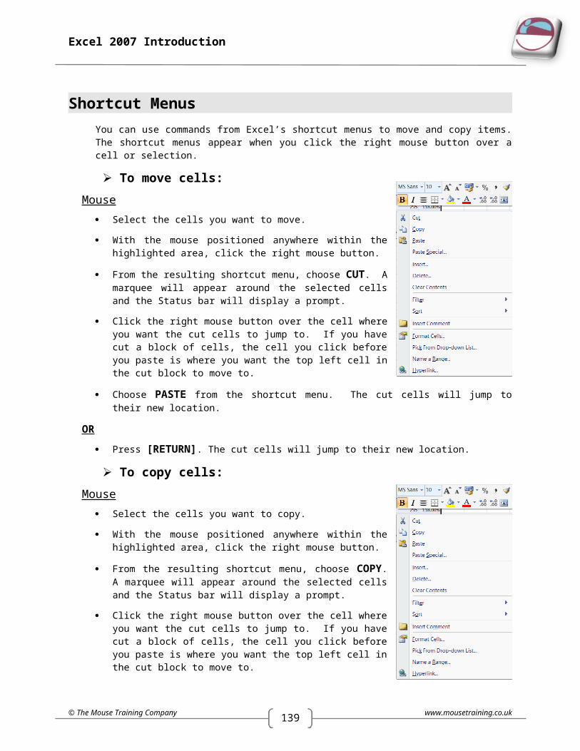
140
Excel 2007 Introduction
AUTOFIT
If you’re not sure what the optimum width for a column would be, you can get Excel to AutoFit it for you. AutoFit looks at all the data in a column and fits the column width around the widest entry – you may find the column gets wider or narrower when you AutoFit.
To AutoFit a column:Mouse
Move the mouse over the intersection between the column letters on the right-hand side of the column you want to change. The mouse pointer will display the shape that you need for changing column width.
Double-click the intersection.
To AutoFit multiple columns:Mouse
Select the columns you want to AutoFit by clicking and dragging over the column letters with the selection pointer (white plus).
Position the mouse over one of the intersections between the column letters in your selection. The pointer will display the shape needed for altering column widths.
Double-click to AutoFit all selected columns.
DEFAULT WIDTH
If you need to change Excel’s default width, you can choose an option from the menu to do so and to set a new default for the whole sheet
To change the default column width:Mouse
Click in any column.
Choose Format from the cells group on the home ribbon, and click on default Width.
A dialog box appears. Enter a size and click OK
All columns on that sheet will change to the new size
Any column that has previously had its width changed will be unaffected by this. Because other formats can affect the widths your columns need to be, it is often a good idea to leave changing column widths until last, this will avoid you repeatedly having to change the widths as you apply other formats. If the column of a cell is too narrow to display the numbers, Excel displays the cell with ####. If you hover over the cell a tool tip will appear displaying the information within the cell.
www.mousetraining.co.uk © The Mouse Training Company
139
Excel 2007 Introduction
Row HeightExcel automatically changes row height when you alter the font and point size of the cell entries within it. However, you can alter the height of a single row manually, or by selecting the rows whose height you want to change, you can make all rows in the selection the same height. With a single row, Excel changes the height of the row above your mouse pointer.
To change row height:Mouse
Move the mouse over the intersection between the row numbers below the row you want to change. The mouse pointer will display the shape that you need for changing row height.
Click and drag up or down to increase or decrease row height – a guide will draw itself across into the worksheet to preview where the row edge will jump to, and Excel will display the actual height of the row in points in a tip box that appears.
Release the mouse when the desired height has been reached.
To change height of multiple rows:Mouse
Select the rows whose height you want to change by clicking and dragging over the row numbers with the selection pointer (white plus).
Position the mouse over one of the intersections between the row numbers in your selection. The pointer will display the shape needed for altering row heights.
Click and drag up or down to increase or decrease row height - a guide will draw itself across into the worksheet to preview where the row edge will jump to, and Excel will display the actual height of the rows in points in a tip box that appears.
Release the mouse when the desired height is reached. All the rows in the selection will jump to the same height as the one you changed.
AUTOFIT
If you’re not sure what the optimum height for a row would be, you can get Excel to AutoFit it for you. AutoFit looks at all the data in a row and fits the row height around the tallest entry – you may find the row gets taller or shorter when you AutoFit.
To AutoFit a row:Mouse
Move the mouse over the intersection between the row numbers below the row you want to change. The mouse pointer will display the shape that you need for changing column width.
Double-click the intersection.
© The Mouse Training Company www.mousetraining.co.uk

140
Excel 2007 Introduction
To AutoFit multiple rows:Mouse
Select the rows you want to AutoFit by clicking and dragging over the row numbers with the selection pointer (white plus).
Position the mouse over one of the intersections between the row numbers in your selection. The pointer will display the shape needed for altering row heights.
Double-click to AutoFit all selected rows.
Hide Columns, Rows And SheetsYou can choose not to display certain rows and columns on your screen. Hiding them also prevents them from printing.
To hide columns:Mouse
Select the column you want to hide by clicking on the column letter, or if you want to hide multiple columns, highlight them.
Click the right mouse button anywhere over the selection to display the shortcut menu.
Choose Hide.
OR
Click on FORMAT command in the cell group on the HOME ribbon
Move mouse cursor of HIDE & UNHIDE
Click on hide columns
OR
Keyboard Repeat step 1 above.
Press [CTRL][0]
www.mousetraining.co.uk © The Mouse Training Company
139
Excel 2007 Introduction
To hide rows:Mouse
Select the row you want to hide by clicking on the row number, or if you want to hide multiple rows, highlight them.
Click the RIGHT MOUSE button anywhere over the selection to display the shortcut menu.
Choose HIDE.
OR
Select rows to be hidden
Click on FORMAT command in the CELL group on the HOME ribbon
Move mouse cursor to HIDE & UNHIDE
Click on HIDE ROWS
OR
Keyboard Repeat step 1 above.
Press [CTRL][0]
To hide sheetsMouse
Select sheet or sheets to be hidden
Click on FORMAT command in the CELL group on the HOME ribbon
Move mouse cursor to HIDE & UNHIDE
Click on HIDE SHEET
OR
Select sheets to be hidden
Right click on a selected sheet tab
Click HIDE
© The Mouse Training Company www.mousetraining.co.uk

140
Excel 2007 Introduction
To unhide columns and rows or sheets:Mouse
Select the columns or rows either side of the hidden ones by dragging over the column letters or row numbers with the selection pointer.
Position the mouse over the row or column intersection between the selected rows or columns
Double-click.
OR
Keyboard Repeat step 1 above.
Press [CTRL][SHIFT][].
OR
Mouse
Click on FORMAT command in the cell group on the HOME ribbon
Move mouse cursor to HIDE & UNHIDE
Click on unhide sheet, column or row
INSERT AND DELETE CELLS, ROWS, COLUMNS OR SHEETSYou can add new cells into a worksheet if you need to make space to add new entries in. Excel also gives you tools for adding entire rows and columns. If you add cells, Excel will ask you how the existing cells should be rearranged to accommodate the new ones.
Add Cells
To insert a cell:Mouse
Select the cell below or to the right of where you want the new one.
Click the right mouse button to access the shortcut menu.
Choose Insert. The following dialog box will appear:
Choose SHIFT CELLS RIGHT to insert a new cell to the left of the selected one, or SHIFT CELLS DOWN to insert a new cell above the selected one.
Or
Keyboard Repeat step 1 above.
www.mousetraining.co.uk © The Mouse Training Company
Shift cells right
Shift cells down
Before…
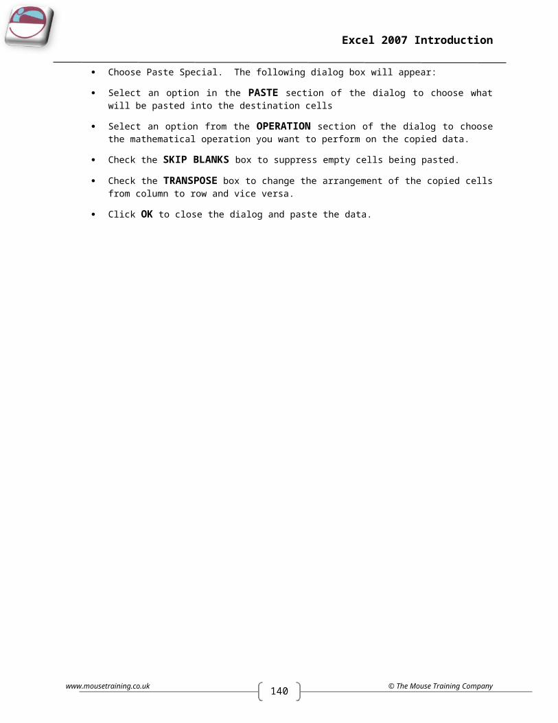
139
Excel 2007 Introduction
Press [CTRL][SHIFT][+]
To insert multiple cells:Mouse
Select the amount of cells corresponding to the number you want to insert below or to the right of where you want the new ones.
Click the right mouse button to access the shortcut menu.
Choose Insert to access the dialog.
Choose SHIFT CELLS RIGHT to insert new cells to the left of the selected one, or SHIFT CELLS DOWN to insert new cells above the selected one.
OR
Keyboard Repeat step 1 above.
Press [CTRL][SHIFT][+].
To insert entire rows:Mouse
Select the row below where you want the new one by clicking its row number, or if you are inserting multiple rows, highlight them.
Click the right mouse button anywhere over the selection to access the shortcut menu.
Choose Insert. Excel adds the number of selected rows above the first row in your selection.
OR
Keyboard
Repeat step 1 above. Then Press [CTRL][SHIFT][+].
To insert entire columns:Mouse
Select the column to the right of where you want the new one by clicking its column letter, or if you are inserting multiple columns, highlight them.
Click the right mouse button anywhere over the selection to access the shortcut menu.
Choose INSERT. Excel adds the number of selected columns to the left of the first column in your selection.
OR
Keyboard Repeat step 1 above.
© The Mouse Training Company www.mousetraining.co.uk
Before…
Shift cells right
Down
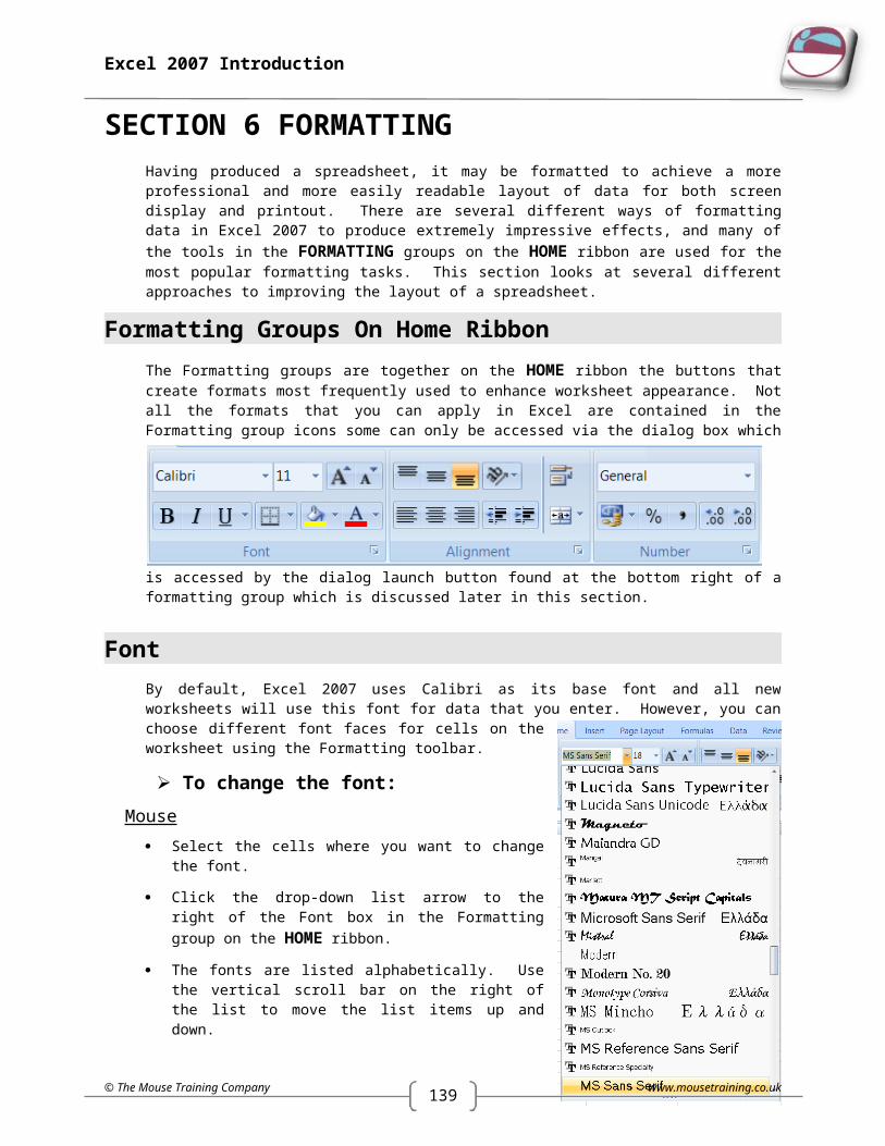
140
Excel 2007 Introduction
Press [CTRL][SHIFT][+].
Delete CellsIn Excel 2007 we can delete straight from the HOME ribbon by clicking on the delete button to show us a menu to delete any part of the workbook, sheet, row, column or cell
To delete cells:Mouse
Select the cells you want to delete.
Click the right mouse button to access the shortcut menu.
Choose DELETE. The following dialog box will appear:
Choose SHIFT CELLS LEFT to close the gap left by the deleted cells with cell entries to the left.
OR
Choose SHIFT CELLS UP to close the gap left by the deleted cells with cell entries above.
OR
Keyboard Select the cells to delete.
Press [CTRL][-].
Choose SHIFT CELLS LEFT to close the gap left by the deleted cells with cell entries to the left.
OR
Choose SHIFT CELLS UP to close the gap left by the deleted cells with cell entries above.
To delete entire rows or columns:Mouse
Select the row or column you want to delete by clicking its row number or column letter or, if you are deleting multiple columns or rows, highlight them.
Click the right mouse button anywhere over the selection to access the shortcut menu.
Choose DELETE.
OR
Keyboard Repeat step 1 above.
Press [CTRL][-]
www.mousetraining.co.uk © The Mouse Training Company
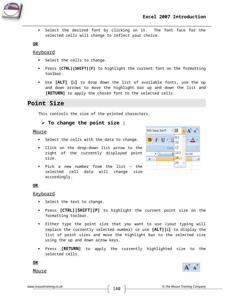
139
Excel 2007 Introduction
FORMAT PAINTERThe Format Painter is a tool that you can use to copy all formats from one area of the worksheet to another. This is particularly useful when you have spent time formatting one group of cells and you decide that another group of cells should have the same formats – rather than reapplying the formats again manually, one by one, you can paint them on to the new cells with the Format Painter.
To paint formats:Mouse
Select the cell that has the formatting you want to use.
Click the FORMAT PAINTER button from the HOME ribbon in the CLIPBOARD group. Your mouse pointer will change to display a paintbrush next to the selection pointer (white plus).
Select all the cells you want to apply the formats to by dragging over them. As soon as you release the mouse, the formats will appear.
If you want to keep cell contents but remove all the formatting from those cells, click on the eraser on the home ribbon and clear formats
Shortcut Keys For FormattingExcel has some shortcut keys that you can use for formatting data. The table below lists those you can use:
To PressDisplay the Cells command (Format menu) [CTRL][1]Apply the General number format [CTRL][SHIFT][~]Apply the Currency format with two decimal places (negative numbers appear in parentheses)
[CTRL][SHIFT][$]
Apply the Percentage format with no decimal places [CTRL][SHIFT][%]Apply the Exponential number format with two decimal places
[CTRL][SHIFT][^]
Apply the Date format with the day, month, and year [CTRL][SHIFT][#]Apply the Time format with the hour and minute, and indicate A.M. or P.M.
[CTRL][SHIFT][@]
Apply the Number format with two decimal places, 1000 separator, and – for negative values
[CTRL][SHIFT][!]
Apply the outline border [CTRL][SHIFT][&]Remove all borders [CTRL][SHIFT][_]Apply or remove bold formatting [CTRL][B]Apply or remove italic formatting [CTRL][I]Apply or remove an underline [CTRL][U]Apply or remove strikethrough formatting [CTRL][5]Hide rows [CTRL][9]Unhide rows [CTRL][SHIFT][9]Hide columns [CTRL][0]Unhide columns [CTRL][SHIFT][+]
© The Mouse Training Company www.mousetraining.co.uk

139
Excel 2007 Introduction
SECTION 7 NAMESWhen entering formulae or referring to any area in a workbook, it is usual to refer to a ‘range’. For example, B6 is a range reference; B6:B10 is also a range reference. One problem with this sort of reference is that it is not very meaningful and therefore easily forgettable. If you want to refer to a range several times in formulae or functions, you may find it necessary to write it down, or select it, which often means wasting time scrolling around the workbook. Instead, Excel offers the chance to name ranges in a workbook, and to use these names to select cells, refer to them in formulae or use them in Database, Chart or Macro commands.
Rules When Naming CellsNames are unique within a workbook and the names that you choose to use must adhere to certain rules.
The first character of a name must be a letter or an underscore character. Remaining characters in the name can be letters, numbers, full stops, and underscore characters.
Names cannot be the same as a cell reference, such as Z$100 or R1C1.
Spaces are not allowed. Underscore characters and full stops may be used as word separators - for example, First.Quarter or Sales_Tax.
A name can contain up to 255 characters.
Names can contain uppercase and lowercase letters. Microsoft Excel does not distinguish between uppercase and lowercase characters in names. For example, if you have created the name Sales and then create another name called SALES in the same workbook, the second name will replace the first one.
Names can refer to external cells or ranges (in other workbooks) and can even be used when those workbooks are not open, although when the references are checked by excel on update errors will occur if they are not valid.
NAME BOX
The Name box is situated on the left-hand side of the Formula bar. You can use the Name box to set up names and move to them.
DEFINE NAME
There are three ways to create names or define them the management of names will be found on the FORMULAS RIBBON in the DEFINED NAMES group.
© The Mouse Training Company www.mousetraining.co.uk
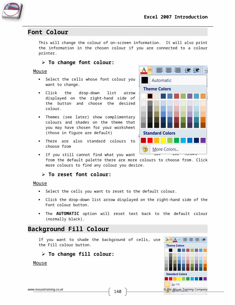
140
Excel 2007 Introduction
To define a name
Method 1 (Define)Mouse
Select the cell or cells you wish to name
Click the DEFINE NAME from the DEFINED NAMES group on the FORMULAS ribbon. A dialog is launched
In the NEW NAME dialog box, in the NAME box, type the name that you want to use for your reference. Names can be up to 255 characters in length.
In the name box, enter the defined name that you want to create.
To specify the scope of the name, in the SCOPE drop-down list box, select WORKBOOK, or the name of a worksheet in the workbook.
You may enter a descriptive comment up to 255 characters. This is optional (see note)
If you had selected cells or ranges previous to opening the NEW NAME dialog then the cells or ranges selected will be displayed in the REFERS TO box
If you had not previously selected cells or ranges: Then In the REFERS TO box
Enter a CELL REFERENCE. The current selection is entered by default. To enter other cell references as an argument, click COLLAPSE DIALOG (which temporarily hides the dialog box), select the cells on the worksheet, and then press EXPAND DIALOG.
CONSTANT Type an = (equal sign), followed by the constant value.
FORMULA Type an = (equal sign) followed by the formula. To finish and return to the worksheet, click OK.
If you save the workbook to Microsoft Office SharePoint Server 2007 Excel Services, and you specify one or more parameters, the comment is used as a tooltip in the PARAMETERS toolpane.
To make the New Name dialog box wider or longer, click and drag the grip handle at the bottom.
Method 2 (Direct)Mouse
Select the cell, range of cells, or nonadjacent selections (nonadjacent selection: A selection of two or more cells or ranges that don't touch each other. When plotting nonadjacent selections in a chart, make sure that the combined selections form a rectangular shape.) that you want to name.
Click in the NAME BOX at the left end of the formula bar(formula bar: A bar at the top of the Excel window that you use to enter or edit values or formulas in cells or charts. Displays the constant value or formula stored in the active cell.).
Type the name that you want to use to refer to your selection. Names can be up to 255 characters in length and press RETURN.
www.mousetraining.co.uk © The Mouse Training Company

139
Excel 2007 Introduction
You cannot name a cell while you are changing the contents of the cell.
Method 3 (By Selection)MOUSE
You can convert existing row and column labels to names.
Select the range that you want to name, including the row or column labels.
On the FORMULAS tab, in the DEFINED NAMES group, click CREATE FROM SELECTION.
In the CREATE NAMES FROM SELECTION dialog box, designate the location that contains the labels by selecting the TOP ROW, LEFT COLUMN, BOTTOM ROW or RIGHT COLUMN check box.
Press ENTER.
Selecting Names (Navigation)Names have great uses as a navigation tool within a document and are very easy to use . You may have used large portions of your spreadsheet to store data and with over 1,000,000 rows and 0ver 16,000 columns it would be tedious or near impossible to move around to known areas without names.
To select names and navigateMouse
Click on drop down arrow to right of name box and click on the name you would like to navigate to
You will now be at that location with the named cells selected
© The Mouse Training Company www.mousetraining.co.uk
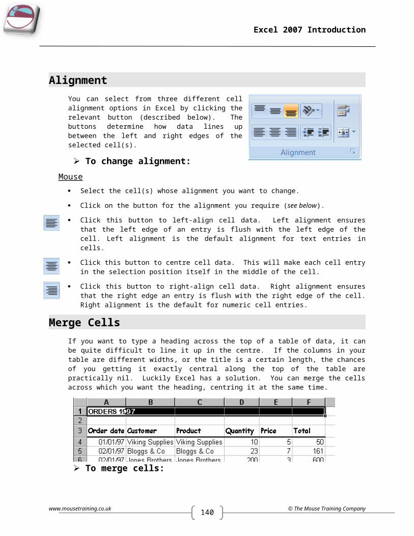
140
Excel 2007 Introduction
Manage Names By Using The Name Manager.Use the NAME MANAGER Dialog box to work with all of the defined names and table names in the workbook. For example, you may want to find names with errors, confirm the value and reference of a name, view or edit descriptive comments, or determine the scope. You can also sort and filter the list of names, and easily add, change, or delete names from one location.
To use name managerMouse
To open the NAME MANAGER Dialog box, on the FORMULA tab, in the DEFINED NAMES group, click NAME MANAGER.
VIEW NAMES
The NAME MANAGER Dialog box displays the following information about each name in a list box:
ICON and NAME defined name is indicated by a defined name icon.
A TABLE NAME is indicated by a table name icon.
If you save the workbook to Microsoft Office SharePoint Server 2007 Excel Services, and you specify one or more parameters, the comment is used as a tooltip in the Parameters toolpane.
You cannot use the Name Manager Dialog box while you are changing the contents of the cell.
The Name Manager Dialog box does not display names defined in Visual Basic for Applications (VBA), or hidden names (the visible property of the name is set to "False").
www.mousetraining.co.uk © The Mouse Training Company

139
Excel 2007 Introduction
RESIZE COLUMNS
To automatically size the column to fit the largest value in that column, double-click the right side of the column header.
SORT NAMES
To sort the list of names in ascending or descending order, alternately click the column header.
FILTER NAMES
Use the commands in the FILTER drop-down list to quickly display a subset of names. Selecting each command toggles the filter operation on or off, which makes it easy to combine or remove different filter operations to get the results that you want.
To filter the list of names, do one or more of the following:
Select: To:
Names Scoped To Worksheet Display only those names that are local to a worksheet.
Names Scoped To Workbook Display only those names that are global to a workbook.
Names with Errors Display only those names with values that contain errors (such as #REF, #VALUE, #NAME, and so on.)
Names without Errors Display only those names with values that do not contain errors.
Defined Names Display only names defined by you or by Excel, such as a print area.
Table Names Display only table names.
To Change a nameMouse
On the FORMULAS tab, in the DEFINED NAMES group, click NAME MANAGER.
In the NAME MANAGER Dialog box, click the name that you want to change, and then click Edit. You can also double-click the name.
The EDIT NAME dialog box is displayed.
Type the new name for the reference in the NAME box.
Change the reference in the REFERS TO box, and click OK.
In the NAME MANAGER Dialog box, in the REFERS TO box, change the cell, formula or constant represented by the name.
To cancel unwanted or accidental changes, click CANCEL , or press ESC.
To save changes, click COMMIT , or press RETURN.
If you change a defined name or table name, all uses of that name in the workbook are also changed. The CLOSE button only closes the NAME MANAGER Dialog box. It is not required to commit changes that have already been made.
© The Mouse Training Company www.mousetraining.co.uk

140
Excel 2007 Introduction
Delete one or more names On the FORMULAS tab, in the DEFINED NAMES group, click NAME MANAGER.
In the NAME MANAGER Dialog box, click the name that you want to change.
To select a name, click it.
To select more than one name in a contiguous group, click and drag the names, or press [SHIFT][CLICK] for each name in the group.
To select more than one name in a non-contiguous group, press [CTRL][CLICK] for each name in the group.
Click DELETE. You can also press DELETE.
Click OK to confirm the deletion.
The Close button only closes the Name Manager Dialog box. It is not required to commit changes that have already been made.
Names In FunctionsNames in functions can be very useful because it saves you having to go and select large amounts of cells or ranges when constructing a function you can just refer to the name and even then remembering the name is not necessary it can be selected and used easily within your function or formula.
To use names in functions Go to cell you wish to create formula in and type in the function you wish to start with
E.G. =SUM(
On the FORMULAS tab, in the DEFINED NAMES group, click USE IN FORMULA.
Select which named range you wish to use and click on it.
OR
Press [F3], choose the name you require and click OK
www.mousetraining.co.uk © The Mouse Training Company

139
Excel 2007 Introduction
The function will now contain the named range and will calculate using the range or ranges it refers to
Press ENTER. Or click on the green tick on the left of the FORMULA BAR.
You may wish to use other methods to create your function or formulae only one method is mentioned here but it is the same method for using the named ranges
Paste List Of NamesYou can use the Paste Names dialog to give you an index of all the names in your workbook. Excel will place this on the workbook wherever the active cell is positioned.
To paste a list of names:Mouse
On the FORMULAS tab, in the DEFINED NAMES group, click USE IN FORMULA.
Click on PASTE NAMES a dialog box is launched
Select an individual name and click on OK for an individual paste.
OR
Click on PASTE NAMES to have all names pasted into worksheet with their cell references
Keyboard Select a blank cell where you want the list of names to begin.
Press [F3] to access the Paste Names dialog.
Press [TAB] to jump to the Cancel button, then [TAB] again to select the Paste List button. The list will appear on the worksheet.
When you choose a start cell for your pasted list, make sure there is not any data immediately below as it will get cleared when you paste the list.
Intersecting NamesWhere you have named both columns of cells and rows of cells in a table, all the values will belong to two ranges. You can use both names in a formula to retrieve the value where they intersect.
To display a value from intersecting range names:Keyboard
Select the cell where you want to display the value.
Type an equals sign (=) to begin the formula then press [F3] to access the PASTE NAMES dialog, select the first name and press [RETURN].
© The Mouse Training Company www.mousetraining.co.uk
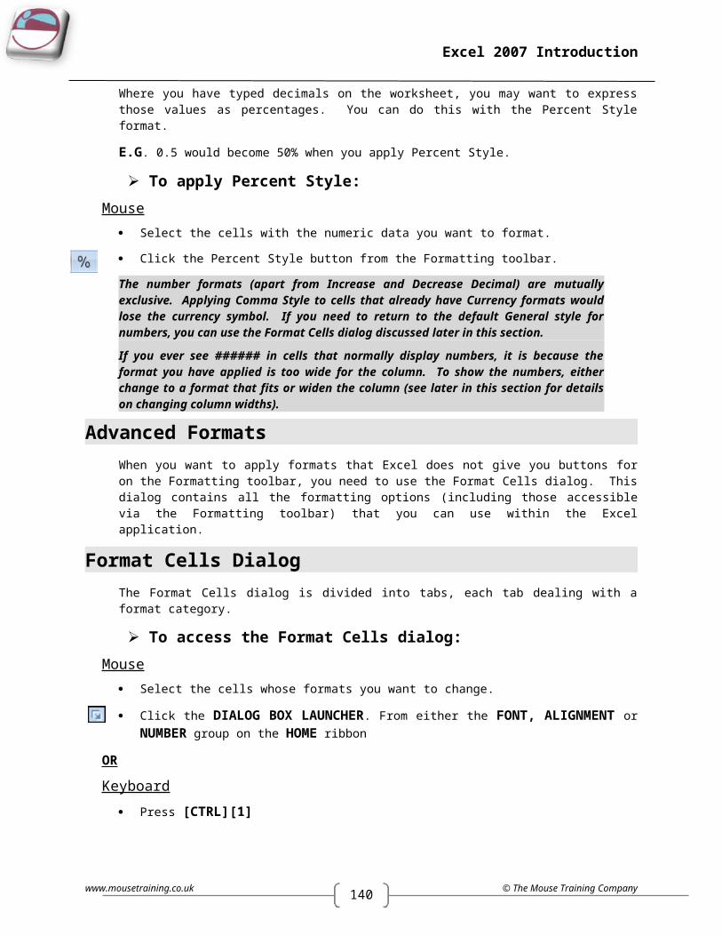
140
Excel 2007 Introduction
Type a space. Press [F3] again and select the second name. Press [RETURN]. Press [RETURN] again to complete the formula.
E.G.: To retrieve the red books target figure from the data shown in the diagram above, your formula would read: =RED_BOOKS TARGET
www.mousetraining.co.uk © The Mouse Training Company

139
Excel 2007 Introduction
SECTION 8 WORKING WITH MULTIPLE SHEETS
MULTIPLE WORKSHEETSWhen you create a new workbook, Excel gives you multiple pages within that workbook called worksheets. The number of worksheets you get defaults to 3, but you can change that (see the section on customisation for more information). The worksheets are useful when you want to store information under common column headings but need to split it up, (for example by month, week or by department).
When the same data needs to be entered on several worksheets, you can use Group mode which forces data that you type on one worksheet appear on all selected sheets. When Group mode is active, any formatting that you apply to the active worksheet also gets applied to the selected sheets.
Moving Between The Workbook SheetsEach new workbook contains worksheets, named sheets 1 to sheet 3. The sheet name appears on a tab at the bottom of the workbook window.
To move between worksheets:Mouse
Click on the appropriate tab
If the sheet required is not in view, use the tab scrolling buttons to display the sheet.
OR
Keyboard
Press [CTRL][PAGE DOWN] to move to the next sheet, or [CTRL][PAGE UP] to move to the previous sheet.
Worksheet NamesExcel assigns the names “Sheet 1, Sheet 2” and so on to worksheets in a workbook but you can overwrite them with more meaningful names to describe the data they contain.
To rename a worksheet:Mouse
Double-click the sheet tab that you want to rename – the current name will become highlighted.
Type the name you want.
Press [RETURN].
Worksheet names can be a maximum of 31 characters.
© The Mouse Training Company www.mousetraining.co.uk
Tab scrolling buttons
Create new sheet

140
Excel 2007 Introduction
Move And Copy WorksheetsHaving named your sheets, you may need to switch them about so they are arranged in a different order.
To move a sheet:
Mouse Click and drag the sheet tab left or right. You’ll see a page which follows your mouse pointer as you
drag and a black marker arrow to show where the sheet will jump to if you release the mouse.
Release the mouse when the sheet is in the correct position.
To copy a worksheet:
Mouse
Hold down the [CTRL] key then click and drag the sheet tab.
When the black arrow marker indicates the position that you want the copy, release the mouse then the [CTRL] key.
Because no 2 worksheets can have the same name, when you copy a sheet as described above, Excel will suffix the copy’s name with (2).
Insert And Delete WorksheetsYou can add and remove worksheets to and from a workbook as required.
To add a worksheet:Mouse
Click on the last tab of the sheets this is a create new worksheet tab
Excel will name it initially with the next sequential number available.
OR
Keyboard
Press [SHIFT][F11]
A new sheet will appear the tab will be to the left of whichever sheet you are currently on and Excel will name it initially with the next sequential number available.
To delete a worksheet:Mouse
Click the right mouse button over the worksheet that you want to delete.
www.mousetraining.co.uk © The Mouse Training Company

139
Excel 2007 Introduction
Choose DELETE from the shortcut menu. If there has been ANY work on the sheet to be deleted the following dialog box will appear:
Click OK to confirm the deletion.
© The Mouse Training Company www.mousetraining.co.uk

140
Excel 2007 Introduction
ACTIVATE GROUP MODEWhenever you select more than one worksheet, Excel considers those sheets to be grouped and switches group mode on accordingly. When group mode is active, the grouped worksheet tabs turn white and the word “[group]” appears on the title bar. Any data that you enter and any formatting that you apply will appear on all worksheets in the group in the same positions on each – this is particularly useful if you need to create a “Summary” sheet that will reference the other worksheets three dimensionally.
Group Adjacent SheetsWhen the worksheets that you want to group are next to each other, you can use the [SHIFT] key to block select them.
To group adjacent worksheets:Mouse
Click the on the first worksheet’s tab that you want to include in your group.
Hold down the [SHIFT] key and click on the last worksheet’s tab that you want included in your group. All the sheets between the first and the last will be selected. The selected sheet tabs will turn white and the word “[GROUP]” will appear on the title bar.
Group Non-Adjacent SheetsWhen the sheets you want are not next to each other in the workbook, you can use the [CTRL] key to group them.
To group non-adjacent worksheets:Mouse
Click the on the first worksheet’s tab that you want to include in your group.
Hold down the [CTRL] key and click each other worksheet’s tab that you want included in your group. The selected sheet tabs will turn white and the word “[GROUP]” will appear on the title bar.
When worksheets are grouped, use normal data entry and formatting commands to populate them (see previous sections for more information).
Deactivate Group ModeWhen you have finished entering and formatting data simultaneously, you can deactivate group mode. There are two ways to do this:
To deactivate group mode:Mouse
Click on a sheet tab that is not currently grouped (non white).
OR
Click the right mouse button over any sheet tab and choose Ungroup Sheets from the shortcut menu.
www.mousetraining.co.uk © The Mouse Training Company
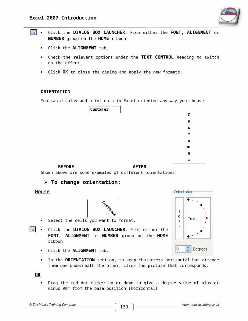
139
Excel 2007 Introduction
FILL DATA ACROSS WORKSHEETSYou can copy data to the same position on multiple sheets using the Fill command. This is particularly useful if you need to decide what gets copied (everything, or just the formats). It also saves time for those occasions where you accidentally deactivated group mode, typed your entries and then realised that they are only on one page!
To fill across worksheets:Mouse
Select the cells you want to copy to the other worksheet(s).
Select the worksheets you want the copy to appear on by clicking the sheet tabs (use [SHIFT] to block select or [CTRL] to pick non-adjacent pages).
On the FORMULAS tab, in the EDITING group, click the down arrow to the right of the FILL icon.
Choose across worksheets
Choose the appropriate option and click OK.
When you have finished filling the data, remember to deactivate group mode!
3-D FormulaeWhen you have data on multiple worksheets, you often want a summary page that will collect data from cells across all the sheets and calculate it in a certain way. You can do this with a 3-D formula. 3-D formulae are no different from the formulae already discussed in an earlier section of this manual, however, the way you refer to cells on different worksheets has not yet been explored – that is what we will look at in this section.
© The Mouse Training Company www.mousetraining.co.uk

140
Excel 2007 Introduction
External ReferencesWhen you refer to a cell that is in another worksheet, Excel uses the following syntax:
SINGLE CELL
‘WORKSHEET NAME’![CELL REFERENCE]
In the diagram on previous page, cell D35 on the Summary sheet would be referenced as follows:
‘SUMMARY’!D35
CELLS ON ADJACENT WORKSHEETS
1STWORKSHEET NAME:LASTWORKSHEET NAME![CELL REFERENCE]
In the diagram on previous page, cell E32 across all staff would be referenced:
CONNERS:PULASKI!E32
CELLS ON NON-ADJACENT WORKSHEETS
1ST WORKSHEET NAME![CELL REFERENCE],2ND WORKSHEET NAME![CELL REFERENCE]
In the diagram, cell D35 on Connor’s and Fuller’s sheets would be referenced:
CONNERS!D35,FULLER!D35
Luckily, because you can get Excel to put the references in automatically by pointing at the cells, you do not have to memorise the syntax!
Commas separate up the references when selecting ranges or cells in this manner from different sheets
To create a 3-D formula:Mouse
Select the cell where you want the result.
Begin the formula by typing an equals sign (=), or select a function that you want to use.
When you need to enter cell references in your formula, move to the worksheet that contains the first cell you want by clicking the relevant sheet tab.
Click on the cell whose value you want in your formula.
www.mousetraining.co.uk © The Mouse Training Company

139
Excel 2007 Introduction
If you only need to refer to one cell, press [RETURN] to complete the formula.
OR
If you need to select the same cell on adjacent sheets, hold down the [SHIFT] key and click on the last sheet tab in the block of adjacent sheets. Press [RETURN] to complete the formula.
OR
If you need to select the different cells on different sheets, TYPE A COMMA and click the next sheet tab and cell you need to reference, insert another comma and click the next sheet tab and cell you need to reference and so on until all references have been entered. Press [RETURN] to complete the formula.
© The Mouse Training Company www.mousetraining.co.uk
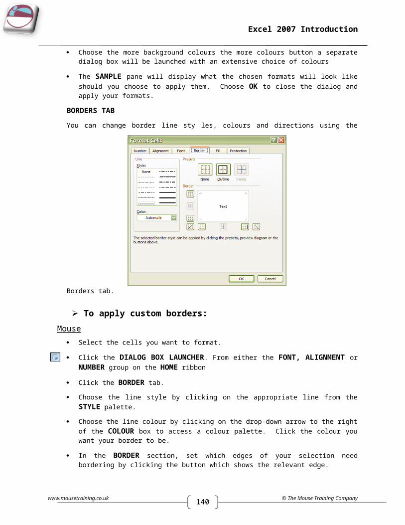
140
Excel 2007 Introduction
PROTECT WORKSHEET DATAIf you type in a cell that already has an entry, you overwrite that entry as soon as you press [RETURN]. Excel does have an Undo facility, but if you need to delegate data entry to someone who is not too familiar with Excel, they could quite feasibly end up overwriting your carefully constructed formulae. To prevent that happening, you can protect worksheets in workbooks. Protected sheets can allow access to some cells but not others. Those that are unavailable cannot be edited, formatted or cleared.
Unlock CellsBy default, all cells in a worksheet are locked. This does not have any effect on data entry and editing until you switch on the worksheet protection at which point all locked cells are made unavailable. This means that if you want to have access to certain cells, but not others, you need to unlock those cells first.
In the diagram below, you would need to unlock the selected cells so that when you protect the worksheet, those cells are accessible.
www.mousetraining.co.uk © The Mouse Training Company
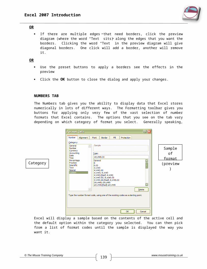
139
Excel 2007 Introduction
To unlock cells:Mouse
Select the cells you want to be accessible when you protect the worksheet – you can select cells on multiple sheets using group mode if necessary.
Click the DIALOG BOX LAUNCHER. From either the FONT, ALIGNMENT or NUMBER group on the HOME ribbon
Click the PROTECTION tab. And uncheck the LOCKED box.
Click OK to close the dialog and save the setting.
OR
Select the cells you want to be accessible when you protect the worksheet – you can select cells on multiple sheets using group mode if necessary.
Click the FORMAT button in the CELLS group on the HOME ribbon. (See picture on previous page)
The LOCK CELL button is already selected (all cells are locked by default). Click the LOCK CELL button to unlock the selected cells.
Worksheet Protection
To protect a worksheet: Mouse
Ensure that the sheet you want to protect is the active sheet.
Click the FORMAT button in the CELLS group on the HOME ribbon. (See picture on previous page). Click on PROTECT SHEET. A dialog box is launched
Select from the checkboxes what you wish people be allowed to do (best left as default) Ticking the FORMAT CELLS option would then allow all users to change the formatting of cells (locked or unlocked) while still preventing them from changing the actual contents of the locked cells.
Type a password to prevent unauthorized users from removing sheet protection. A password is case sensitive, can be up to 255 characters long, and can contain any combination of letters, numbers, and symbols.
Click OK to close the dialog and switch on sheet protection.
RECORD ALL PASSWORDS SOMEWHERE AS DATA CAN BE LOST IF YOU CANNOT REMEMBER THEM With worksheet protection active, only the unlocked cells are available to work with. If you try and type in a locked cell, the following warning appears:
© The Mouse Training Company www.mousetraining.co.uk

140
Excel 2007 Introduction
Unprotect SheetsIf you do need access to the locked cells, you can switch worksheet protection off, provided you know the correct password.
To switch off sheet protection:Mouse
Select the protected sheet.
Click the FORMAT button in the CELLS group on the HOME ribbon. Click on UNPROTECT SHEET.
If you had a password then a dialog box will appear Type the password and click OK. The sheet is now unprotected.
Excel only lets you protect and unprotect sheets one at a time, that is to say, you cannot group all the sheets you want to protect or unprotect and do it in one go.
View Worksheets Side By SideYou can display several worksheets in a workbook tiled in various ways on screen. These options can be found on the VIEW ribbon and the WINDOW group.
To display worksheets side by side:Mouse
Go to the VIEW ribbon and click on the SIDE BY SIDE button a dialog is launched
Choose a file you wish to compare with and see side by side
Click OK
Repeat the above steps until you have a window for each worksheet.
On the VIEW ribbon, click Arrange all. The Arrange Windows dialog box will appear:
Choose the arrangement you want your worksheet windows to follow. Check the box WINDOWS OF ACTIVE WORKBOOK (this prevents windows from other open files being included in the arrangement).
Click OK to close the dialog and arrange the windows.
If your initial window is maximised, you do not see any change to the screen when you issue the New Window command, you may not know how many windows you have. When you access the Window menu, the bottom section lists the number of windows currently open.
www.mousetraining.co.uk © The Mouse Training Company

139
Excel 2007 Introduction
Picture above shows tiled windows
When the windows are opened with the method mentioned previously, the button for synchronous scrolling will allow simultaneous scrolling for all windows. If this feature does not help it can be switched off.
Hide WindowsWhole windows can be hidden. Although you may need them open for calculations, macros, referred tables, etc you may not wish to see them.
To hide a windowMouse
Select the window you wish to hide
Go to the VIEW ribbon and click the HIDE button in the WINDOW group. The window is now hidden
To unhide a window Mouse
Go to the VIEW ribbon and click the UNHIDE button. In the WINDOW group a dialog is launched
Choose window to unhide and click OK. The window reappears.
© The Mouse Training Company www.mousetraining.co.uk

140
Excel 2007 Introduction
Watch WindowA watch window can be used to easily track results of multiple cells when you are working on a different sheet or workbook. This saves you from having to switch back and forth or scroll between sheets to keep track of important data.
To set a watchMouse
Select a cell to which you want to add a Watch
Go to the FORMULAS ribbon an click on WATCH WINDOW in the FORMULA AUDITING group
Click on ADD WATCH
Select cell you wish to monitor
Click on ADD
You may now switch windows or scroll and the watch window will monitor that cell for changes in result as you enter or manipulate figures elsewhere.
To delete a watchMouse
Go to the FORMULAS ribbon an click on WATCH WINDOW in the FORMULA AUDITING group
Select watch to delete
Click on DELETE WATCH on watch window
www.mousetraining.co.uk © The Mouse Training Company
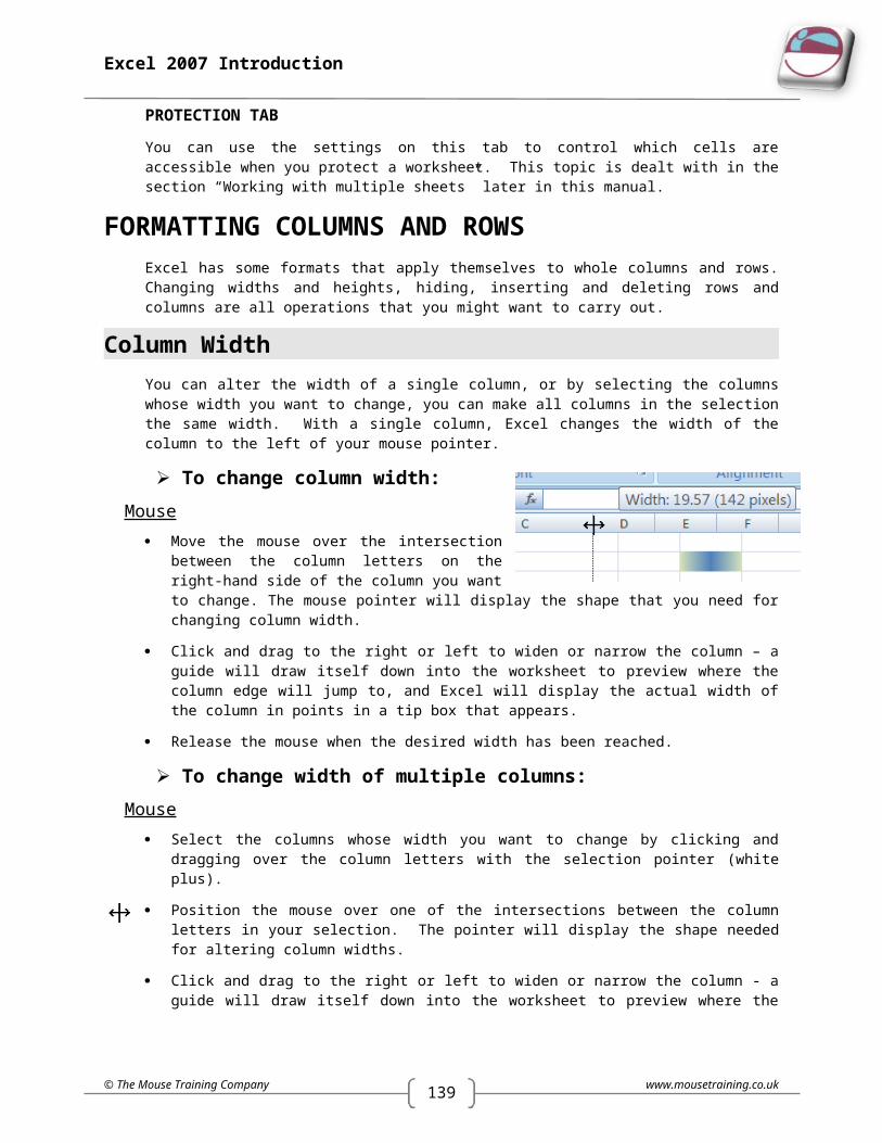
139
Excel 2007 Introduction
Change Colour Of Worksheet Tab
To change the colour of a worksheet tab: Select the worksheet whose tab you want to re-colour.
Click the FORMAT button in the CELLS group, HOME ribbon and move your cursor down the menu to TAB COLOUR.
Select the colour and click OK
OR
Right-click on the tab and choose the TAB COLOUR option.
Select the colour and click OK
© The Mouse Training Company www.mousetraining.co.uk

139
Excel 2007 Introduction
SECTION 9 PRINTINGWhen you want a hard copy of worksheet data, Excel gives you many tools for choosing how that printout will look. Swapping the page orientation between portrait and landscape, scaling the size of the printout and choosing whether to print worksheet gridlines are but a few of the options that can be set. Excel automatically assigns headers and footers to your worksheet data, but you can change or enhance these very easily.
PRINT PREVIEWBefore sending anything to print, it is always a good idea to preview what you will see on the page. The Print Preview window will show how your data is going to print.
To go to print previewMouse
Click the worksheet that you want to preview before you print it.
Click the MICROSOFT OFFICE BUTTON , click the arrow next to PRINT and then click PRINT PREVIEW.
OR
Keyboard
Press [CTRL][F2]. On the PRINT PREVIEW tab, do one or more of the following:
To preview the next and previous page, in the PREVIEW group, click NEXT PAGE and PREVIOUS PAGE.
To view page margins, in the PREVIEW group, select the SHOW MARGINS check box.
This displays the margins in the PRINT PREVIEW view. To make changes to the margins, you can drag the margins to the height and width that you want. You can also change the column widths by dragging handles at top of print preview page.
To make page setup changes, on the Print Preview tab, in the Print group, click Page Setup, and then select the options that you want on the Page, Margins, Header/Footer, or Sheet tab of the Page Setup dialog box.
© The Mouse Training Company www.mousetraining.co.uk
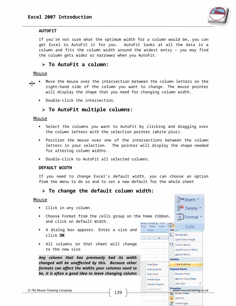
140
Excel 2007 Introduction
PAGE SETUPWhen you want to alter headers and footers, orientation and so on, you use the Page Setup dialog box. There are four tabs within this dialog, each give settings for one aspect of your printout. You can access the Page Setup dialog from either the worksheet or the Print Preview window, however if you access it from the latter, some of the SHEET tab settings are unavailable.
PAGE SETUP GROUP ON THE PAGE LAYOUT RIBBON
To access the page setup dialog:Mouse
Click the DIALOG BOX LAUNCHER. From PAGE SETUP group on the PAGE LAYOUT ribbon
OR
If you are in the Print Preview window, click the PAGE SETUP button
PAGE TAB
The PAGE tab allows you to set page orientation, scaling, paper size, print quality and a start number for page numbering.
ORIENTATION
www.mousetraining.co.uk © The Mouse Training Company

139
Excel 2007 Introduction
Use this setting to swap between portrait and landscape printouts.
To change page orientation:Mouse
Access the PAGE SETUP dialog and click the PAGE tab.
The default orientation is PORTRAIT. Click LANDSCAPE to switch to printing on a landscape page.
Click OK to close the dialog and save the setting – next time you access PRINT PREVIEW, the new settings will be displayed.
OR
Go to PAGE SETUP group on the LAYOUT ribbon and select ORIENTATION. Choose portrait or landscape
SCALING
You can manually scale the size of your printout by choosing a percentage amount you want to increase or decrease it by. The Adjust to option reduces or enlarges the printed worksheet. The Fit to option will only reduce (not enlarge) the worksheet or selection when you print so that it fits on the specified number of pages.
To reduce or enlarge your printout:Mouse
Access the Page Setup dialog and click the PAGE tab.
Select the ADJUST TO check box, and then enter a percentage number in the % normal size box. You can reduce the worksheet to 10 percent of normal size or enlarge it to 400 percent of normal size.
Click OK to close the dialog and save the setting – next time you access Print Preview, the new settings will be displayed.
To fit your printout to a number of pages:Mouse
Access the Page Setup dialog and click the PAGE tab.
Select the FIT TO check box and then enter a number in the PAGE(S) WIDE BY box. If you want to limit the number of pages tall, enter a number in the TALL box.
Click OK to close the dialog and save the setting – next time you access Print Preview, the new settings will be displayed.
© The Mouse Training Company www.mousetraining.co.uk
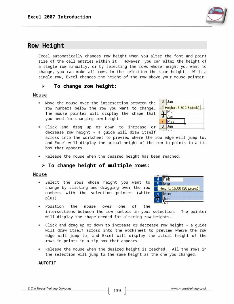
140
Excel 2007 Introduction
PAPER SIZE
You can pick the size of the paper you want to print on by choosing from a list of pre-defined sizes.
To choose paper size:Mouse
Access the Page Setup dialog and click the PAGE tab.
Click the drop-down list arrow to the right of the PAPER SIZE box and click the paper size you want.
Click OK to close the dialog and save the setting – next time you access Print Preview, the new settings will be displayed.
OR
Go to the PAGE SETUP group on the LAYOUT ribbon and click on the SIZE button to see many predefined sizes to set your paper size to. If the size you wish is not available in the list. Then click on MORE PAPER SIZES at the bottom. This launchs the PAGE SETUP dialog box
PRINT QUALITY
You can enhance the quality of the printout if you need a pristine copy.
To change print quality:Mouse
Access the Page Setup dialog and click the PAGE tab.
Click the drop-down list arrow to the right of the PRINT QUALITY box and click the resolution you want for the print quality of the active workbook.
Click OK to close the dialog and save the setting – next time you access Print Preview, the new settings will be displayed.
Resolution is the number of dots per linear inch (dpi) that appear on the printed page. Higher resolution produces better quality printing in printers that support higher resolution printing.
SET FIRST PAGE NUMBER
If your printout is to form part of a larger document, you may need to change start number for pages.
To change first page number: Mouse
Access the Page Setup dialog and click the PAGE tab.
Drag across the word Auto in the FIRST PAGE NUMBER box to select it. Type the number you want the page numbering to begin at.
www.mousetraining.co.uk © The Mouse Training Company

139
Excel 2007 Introduction
Click OK to close the dialog and save the setting – next time you access Print Preview, the new settings will be displayed.
Margins TabThe Margins tab lets you set top, bottom, left and right margins and centre your data horizontally and vertically on the page. You can also determine how far from the bottom and top edges of the page your headers and footers print.
To change margins:Mouse
Access the Page Setup dialog and click the MARGINS tab. (above)
Use the up and down arrows in the TOP, BOTTOM, LEFT and RIGHT boxes to increase and decrease margin measurements. The page sample in the middle of the dialog will update to show how your settings will look should you choose to apply them.
Click OK to close the dialog and save the settings – next time you access Print Preview, the new settings will be displayed.
OR
Go to the LAYOUT ribbon and the PAGE SETUP GROUP and click on margins a selection of quick margin changes will be available including the last custom settings for a page
Click on a set of margins and they will be set.
© The Mouse Training Company www.mousetraining.co.uk

140
Excel 2007 Introduction
To change header and footer position:Mouse
Access the PAGE SETUP dialog and click the MARGINS tab.
Use the up and down arrows in the HEADER and FOOTER boxes to increase and decrease the space between the header and footer and the top and bottom edges of the page.
Click OK to close the dialog and save the settings – next time you access PRINT PREVIEW, the new settings will be displayed.
CENTRE ON PAGE
Use these check boxes to centre the data you are printing horizontally (between left and right margins) and/or vertically (between top and bottom margins).
To centre horizontally and vertically:Mouse
Access the PAGE SETUP dialog and click the MARGINS tab.
Click the HORIZONTALLY check box to centre between left and right margins. Click the VERTICALLY check box to centre between top and bottom margins.
Click OK to close the dialog and save the settings – next time you access PRINT PREVIEW, the new settings will be displayed.
www.mousetraining.co.uk © The Mouse Training Company

139
Excel 2007 Introduction
Header/Footer TabUnless you specify otherwise, Excel uses the sheet name as the header for your printout and the page number as the footer. You can choose from a predefined list of options for your header and footer, or for total flexibility, you can build up the header and footer with codes that will generate dates, times, file names etc.
HEADER
Excel’s default header is the sheet name. The HEADER box gives a list of options for you to use as your header. Excel spaces items out in the header at the top left, middle and top right of the page. Where an option has commas separating items Excel will interpret the comma as the spacing symbol.
To change the header:Mouse
Access the Page Setup dialog and click the HEADER/FOOTER tab.
OR
Click the drop-down list arrow to the right of the HEADER box to view a list of predefined headers and click the one you want. The sample area will show you what your choice will look like.
Click OK to close the dialog and save the settings – next time you access Print Preview, the new settings will be displayed.
© The Mouse Training Company www.mousetraining.co.uk
Sample header
and

140
Excel 2007 Introduction
FOOTER
Excel’s default footer is the page number. The FOOTER box, gives you the same options as the header box, but the position of the chosen item will be at the bottom of the page. Excel spaces items out in the footer at the top left, middle and top right of the page. Where an option has commas separating items Excel will interpret the comma as the spacing symbol.
To change the footer: Click the DIALOG BOX LAUNCHER. From PAGE SETUP group on the PAGE LAYOUT ribbon, select
the HEADER/FOOTER tab ,
Click the drop-down list arrow to the right of the FOOTER box to view a list of predefined footers and click the one you want.
Click OK to close the dialog and save the settings – next time you access Print Preview, the new settings will be displayed.
New Methods For Headers And Footers In 2007In Microsoft Office Excel, you can quickly add or change headers or footers to provide useful information in your worksheet printouts. You can add predefined header and footer information or insert elements such as page numbers, the date and time, and the file name.
To define where in the printout the headers or footers should appear and how they should be scaled and aligned, you can choose header and footer options.
For worksheets, you can work with headers and footers in Page Layout view. For other sheet types, such as chart sheets (chart sheet: A sheet in a workbook that contains only a chart. A chart sheet is beneficial when you want to view a chart or a PivotChart report separately from worksheet data or a PivotTable report.), or for embedded charts (embedded chart: A chart that is placed on a worksheet rather than on a separate chart sheet. Embedded charts are beneficial when you want to view or print a chart or a PivotChart report with its source data or other information in a worksheet.), you can work with headers and footers in the PAGE SETUP dialog box.
Insert Specific Elements In A Header Or FooterFor worksheets, you can work with headers and footers in Page Layout view. For other sheet types, such as chart sheets, or for embedded charts, you can work with headers and footers in the PAGE SETUP dialog box.
Add or change the header or footer text for a worksheet in Page Layout viewMouse
Click the worksheet to which you want to add headers or footers, or that contains headers or footers that you want to change.
On the INSERT tab, in the TEXT group, click HEADER & FOOTER.
www.mousetraining.co.uk © The Mouse Training Company

139
Excel 2007 Introduction
Excel displays the worksheet in Page Layout view. You can also click Page Layout View on the status bar to display this view.
To add a HEADER or FOOTER, click the LEFT, CENTER, or RIGHT HEADER OR FOOTER text box at the top or at the bottom of the worksheet page. And either:
Type the text that you want.
Insert a header or footer element if you from the HEADER AND FOOTER ELEMENTS group on the DESIGN ribbon.
To change a HEADER or FOOTER, click the HEADER or FOOTER text box at the top or at the bottom of the worksheet page that contains header or footer text, and then select the text that you want to change.
To start a new line in a HEADER OR FOOTER text box, press RETURN.
To delete a portion of a HEADER OR FOOTER, select the portion that you want to delete in the header or footer text box, and then press DELETE or BACKSPACE. You can also click in the text and then press BACKSPACE to delete the preceding characters.
To return to NORMAL view, click on the worksheet and then click on on the NORMAL VIEW button on the VIEW tab, in the WORKBOOK VIEWS group. You can also click NORMAL on the status bar.
To include a single ampersand (&) within the text of a header or footer, use two ampersands.
E.G., to include "Subcontractors & Services" in a header, type Subcontractors && Services.
To close the HEADERS OR FOOTERS, click anywhere in the worksheet, or press ESC.
Header Or Footer For A Chart
Add or change the header or footer text for a chartMouse
Click the chart sheet or embedded chart to which you want to add headers or footers, or that contains headers or footers that you want to change.
On the INSERT tab, in the TEXT group, click HEADER & FOOTER. Excel displays the Page Setup dialog box.
Click CUSTOM HEADER or CUSTOM FOOTER.
Click in the LEFT SECTION, CENTER SECTION, or RIGHT SECTION box, and then click the buttons to insert the header or footer information that you want in that section.
To add or change the header or footer text, type additional text or edit the existing text in the LEFT SECTION, CENTER SECTION, or RIGHT SECTION box.
To start a new line in a section box, press RETURN.
© The Mouse Training Company www.mousetraining.co.uk

140
Excel 2007 Introduction
To delete a portion of a header or footer, select the portion that you want to delete in the section box, and then press DELETE or BACKSPACE. You can also click in the text and then press BACKSPACE to delete the preceding characters.
To base a custom header or footer on an existing header or footer, click the header or footer in the Header or Footer box.
Add A Predefined Header Or FooterFor worksheets, you can work with headers and footers in Page Layout view. For other sheet types, such as chart sheets or for embedded charts, you can work with the headers and footers in the PAGE SETUP dialog box.
Add a predefined header or footer to a worksheet in Page Layout viewMouse
Click the worksheet to which you want to add a predefined header or footer.
On the INSERT tab, in the TEXT group, click HEADER & FOOTER.
Excel displays the worksheet in PAGE LAYOUT view. You can also click PAGE LAYOUT VIEW on the STATUS BAR to display this view.
Click the left, center, or right header or footer text box at the top or at the bottom of the worksheet page.
Clicking any text box selects the header or footer and displays the HEADER AND FOOTER TOOLS, on the DESIGN tab.
On the DESIGN tab, in the HEADER & FOOTER group, click HEADER or FOOTER, and then click the predefined header or footer that you want.
To return to NORMAL view, on the View tab, in the Workbook Views group, click Normal. You can also click Normal on the status bar.
Add a predefined header or footer to a chart Click the chart sheet or embedded chart to which you want to add a predefined
header or footer.
On the INSERT tab, in the TEXT group, click HEADER & FOOTER.
Click the predefined header or footer in the HEADER or FOOTER group.
Excel displays the PAGE SETUP dialog box.
www.mousetraining.co.uk © The Mouse Training Company
139
Excel 2007 Introduction
Choose The Header And Footer OptionsFor worksheets, you can work with headers and footers in Page Layout view. For other sheet types, such as chart sheets or for embedded charts you can work with headers and footers in the PAGE SETUP dialog box.
Choose the header and footer options for a worksheetMouse
Click the worksheet for which you want to choose header and footer options.
On the INSERT tab, in the TEXT group, click HEADER & FOOTER.
Excel displays the worksheet in Page Layout view. You can also click Page Layout View on the status bar to display this view.
Click the LEFT, CENTER, or RIGHT header or footer text box at the top or at the bottom of the worksheet page.
Clicking any text box selects the HEADER OR FOOTER and displays the Header and Footer Tools, adding the Design tab.
On the DESIGN tab, in the OPTIONS group, SELECT ONE OR MORE OF THE FOLLOWING:
To insert a different header or footer for odd pages on an odd page and for even pages on an even page, select the DIFFERENT ODD & EVEN PAGES check box.
To remove headers and footers from the first printed page, select the DIFFERENT FIRST PAGE check box.
To use the same font size and scaling as the worksheet, select the SCALE WITH DOCUMENT check box. To make the font size and scaling of the headers or footers independent of the worksheet scaling for a consistent display on multiple pages, clear this check box.
To make sure that the header margin or footer margin is aligned with the left and right margins of the worksheet, select the ALIGN WITH PAGE MARGINS check box. To set the left and right margins of the headers and footers to a specific value that is independent of the left and right margins of the worksheet, clear this check box.
To return to NORMAL view, on the VIEW tab, in the WORKBOOK VIEWS group, click NORMAL. You can also click NORMAL on the status bar.
Choose the header and footer options for a chartMouse
Click the chart sheet or embedded chart to which you want to add a predefined header or footer.
On the INSERT tab, in the TEXT group, click HEADER & FOOTER.
Excel displays the Page Setup dialog box.
© The Mouse Training Company www.mousetraining.co.uk
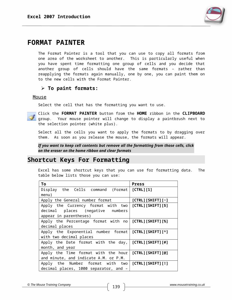
140
Excel 2007 Introduction
To insert a different header or footer for odd pages on an odd page and for even pages on an even page, select the DIFFERENT ODD & EVEN PAGES check box.
To remove headers and footers from the first printed page, select the DIFFERENT FIRST PAGE check box.
To use the same font size and scaling as the worksheet, select the SCALE WITH DOCUMENT check box. To make the font size and scaling of the headers or footers independent of the worksheet scaling for a consistent display on multiple pages, clear this check box.
To make sure that the header margin or footer margin is aligned with the left and right margins of the worksheet, select the ALIGN WITH PAGE MARGINS check box. To set the left and right margins of the headers and footers to a specific value that is independent of the left and right margins of the worksheet, clear this check box.
CUSTOM HEADER AND FOOTER
If none of the predefined headers and footers are what you want, you can customise them using the CUSTOM HEADER and CUSTOM FOOTER buttons. When you click either of these buttons, Excel gives you a dialog box representing either the top (CUSTOM HEADER) or bottom (CUSTOM FOOTER) edge of your page.
You can type text into the left, centre and right sections, but if you want information to change dynamically according to alterations you make to filenames, sheet names or you want to always display the current date and time in the header (useful for seeing when a worksheet was printed),the dialog has buttons that generate codes. The codes instruct Excel to include information where you have positioned them and will update if the information that they generate changes. The diagram below details what each of the buttons do.
OTHER HEADER AND FOOTER SETTINGS
To insert a different header or footer for odd pages on an odd page and for even pages on an even page, select the DIFFERENT ODD & EVEN PAGES check box.
www.mousetraining.co.uk © The Mouse Training Company
Insert PictureFormat PictureFormat
header text
Insert page number
Insert total number of
pagesInsert
current dateInsert
current time
Insert current
filename
Insert sheet name
Inserts the name of the
active worksheet
sheet

139
Excel 2007 Introduction
To remove headers and footers from the first printed page, select the DIFFERENT FIRST PAGE check box.
To use the same font size and scaling as the worksheet, select the SCALE WITH DOCUMENT check box. To make the font size and scaling of the headers or footers independent of the worksheet scaling for a consistent display on multiple pages, clear this check box.
To make sure that the header margin or footer margin is aligned with the left and right margins of the worksheet, select the ALIGN WITH PAGE MARGINS check box. To set the left and right margins of the headers and footers to a specific value that is independent of the left and right margins of the worksheet, clear this check box.
Sheet TabThe Sheet tab has many settings that you can use to select what appears on the printed sheet. You can also use this tab to set a print area, (useful if you do not want the whole worksheet to print) and print titles.
Some settings on the Sheet tab are only available when you access the Page Setup dialog from the LAYOUT ribbon. If you are accessing it from the Print Preview window, you will not have access to the Print Area and Print Titles settings.
PRINT AREA
Use this to set the range of cells that you want to print. If you do not set a Print Area, Excel will print all the data on the active worksheet.
To set a Print Area:Mouse
Click the DIALOG BOX LAUNCHER. From PAGE SETUP group on the PAGE LAYOUT ribbon, select the SHEET tab ,
OR
Click on PRINT AREA From PAGE SETUP group on the PAGE LAYOUT ribbon and select SET PRINT AREA.
© The Mouse Training Company www.mousetraining.co.uk
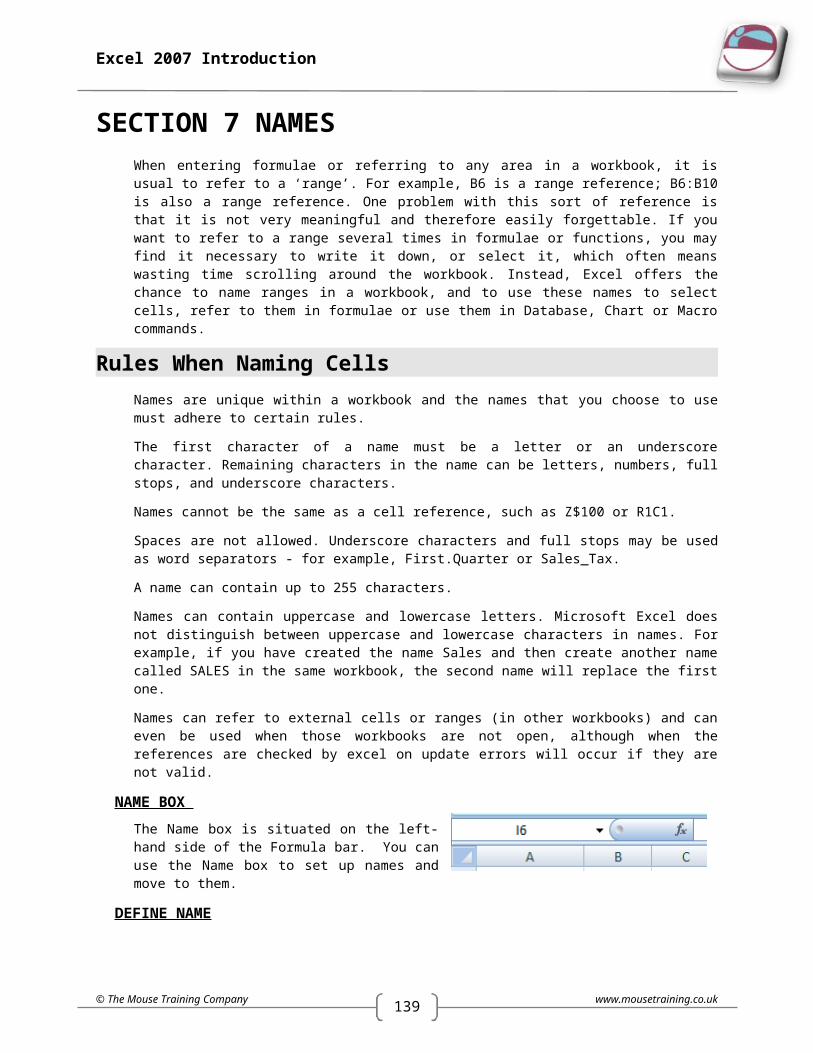
140
Excel 2007 Introduction
Click the button on the right of the PRINT AREA box to collapse the PAGE SETUP dialog so that you can see the worksheet (see below):
Select the cells you want to print and click the EXPAND button to go back to the PAGE SETUP dialog (see below):
The selected cells will appear listed in the PRINT AREA dialog. Click OK to close the dialog and save the settings – next time you access PRINT PREVIEW, the new settings will be displayed.
You can use the Set Print Area option to set the selected cells to the print area as an alternative to using the Page Setup dialog.
To clear the Print Area:Mouse
Click the DIALOG BOX LAUNCHER. From PAGE SETUP group on the PAGE LAYOUT ribbon, select the SHEET tab , Click in the PRINT AREA, Delete the values.
OR
Click on PRINT AREA From PAGE SETUP group on the PAGE LAYOUT ribbon and select CLEAR PRINT AREA.
You can use the Set Print Area option to set the selected cells to the print area as an alternative to using the Page Setup dialog.
www.mousetraining.co.uk © The Mouse Training Company
Click here to expand the dialog

Column titles
Row titles
139
Excel 2007 Introduction
Print TitlesWhen your printouts run to several pages you may have column and row headings that you would like to print on each new page. The diagram below shows a four page printout where the months have been set up to print at the top of each page and the years at the left of each page. Excel allows you to specify any number of rows and columns to repeat when you have a multi-page printout.
To set print titles:Mouse
Access the PAGE SETUP dialog and click the SHEET tab.
OR
Go to the PAGE SETUP group on the PAGE LAYOUT ribbon, and select the PRINT TITLES button. This will open the PAGE SETUP dialog box at the SHEET tab
Click the button on the right of the ROWS TO REPEAT AT TOP box to collapse the Page Setup dialog so that you can see the worksheet (see diagrams) Select the rows you want by dragging over them with the selection pointer.
Click the Expand button to return to the Page Setup dialog. The rows you selected will be referenced in the ROWS TO REPEAT AT TOP box.
Repeat steps (selecting columns not rows) as above for the COLUMNS TO REPEAT AT LEFT box if required.
Click OK to close the dialog and save the settings – next time you access Print Preview, the new settings will be displayed.
© The Mouse Training Company www.mousetraining.co.uk
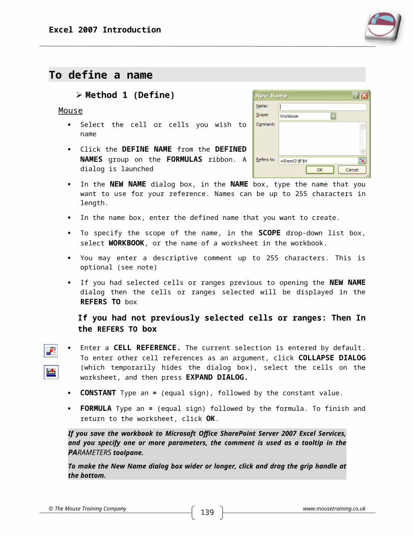
140
Excel 2007 Introduction
The settings here allow you to choose whether to print gridlines, row and column headings and so on. If you choose not to print gridlines, Excel will print any borders you formatted your cells with the diagrams below illustrate some of the effects of activating certain settings.
www.mousetraining.co.uk © The Mouse Training Company
Worksheet with shading…
Black and White
Would print like this.
Gridlines
Worksheet with borders and shading…
Would print like this.
Row headings
Worksheet with row and column headings.

139
Excel 2007 Introduction
To change Sheet tab Print settings: Mouse
Access the Page Setup dialog and click the Sheet tab.
Check the boxes under the PRINT heading until you have the combination of settings that you require.
Click OK to close the dialog and save the settings – next time you access Print Preview, the new settings will be displayed.
PAGE ORDER
When you have multiple pages to print, each with a printed page number, you can control the order that the data prints on the pages using the Page Order settings.
The diagram below shows how pages will have different numbers according to which setting you choose.
To change page order:Mouse
Access the Page Setup dialog and click the SHEET tab.
Click the option button in the PAGE ORDER section for the order you want the pages numbered.
Click OK to close the dialog and save the settings – next time you access Print Preview, the new settings will be displayed.
The Page Setup dialog saves print settings for the active sheet only. If you want several sheets to have the same print settings, select them before you access the Page Setup dialog.
© The Mouse Training Company www.mousetraining.co.uk
Over then down…. Down then over…

140
Excel 2007 Introduction
Page BreaksIf you do not get page breaks to fall where you want them with the scaling options, you can insert them manually. Excel lets you put in both horizontal and vertical page breaks.
To insert a horizontal page break:Mouse
Select the cell in column A below where you want the page break.
Choose breaks from the PAGE SETUP group on the LAYOUT ribbon then click INSERT PAGE BREAK. A dotted line will appear above the active cell – this represents the page break.
To insert a vertical page break:
Mouse Select the cell in row 1 to the right of where you want the page break.
Choose breaks from the PAGE SETUP group on the LAYOUT ribbon then click INSERT PAGE BREAK. A dotted line will appear to the left of the active cell – this represents the page break.
If you insert a page break when you are not in either the first column or row, Excel will insert both a horizontal and vertical page break above and to the left of the active cell position.
To remove a page break:Mouse
Select the cell immediately below and/or to the right of the page break.
Choose breaks from the PAGE SETUP group on the LAYOUT ribbon then click REMOVE PAGE BREAK. The page break will be removed
If RESET ALL PAGE BREAKS is selected then ALL page breaks will be removed
If the Fit To option is active in the page setup dialog, you cannot set manual page breaks.
www.mousetraining.co.uk © The Mouse Training Company

139
Excel 2007 Introduction
Print DataExcel will print all data on the selected worksheet (unless you tell it otherwise by setting a Print Area). If you want to print more than one worksheet, select the sheets you want first, before you click the Print button.
To print the active worksheet:Mouse
Click the worksheet that you want to print.
Click the MICROSOFT OFFICE BUTTON, click the arrow next to PRINT and then click QUICK PRINT this will send everything on the sheet directly to the printer.
OR
Click the worksheet that you want to print.
Click the MICROSOFT OFFICE BUTTON, click the arrow next to PRINT, and then click PRINT this will Launch a dialog box with settings for printing
OR
Keyboard
Press [CTRL][P]. The Print dialog will appear; press [RETURN] to confirm the settings and launch the print. Excel will display a dialog telling you what is printing.
To print a specific worksheet page or range of pages:Mouse
Click the worksheet that you want to print.
Click the MICROSOFT OFFICE BUTTON, click the arrow next to PRINT, and then click PRINT this will Launch a dialog box with settings for printing
OR
Keyboard
Press [CTRL][P].
The following dialog box will appear:
In the PRINT RANGE section of the dialog, click the PAGES option button. A cursor will appear in the FROM box to the right.
© The Mouse Training Company www.mousetraining.co.uk

140
Excel 2007 Introduction
Type in the page number that you want to start at in the FROM box and the end page number in the TO box. Click the OK button to launch the print.
To print the entire workbook: Mouse
Click the MICROSOFT OFFICE BUTTON, click the arrow next to PRINT, and then click PRINT this will Launch a dialog box with settings for printing
OR
Keyboard
Press [CTRL][P].
Click the ENTIRE WORKBOOK option button in the PRINT WHAT section of the dialog.
Click OK to launch the print.
To print the selection:Mouse
Select the cells you want to print.
Click the MICROSOFT OFFICE BUTTON, click the arrow next to PRINT, and then click PRINT this will Launch a dialog box with settings for printing
Click the SELECTION option button in the PRINT WHAT section of the dialog.
Click OK to launch the print.
CopiesBy default, Excel will print one copy of the item you have sent to print. You can print multiple copies by changing the Print dialog settings. When you print multiple copies of a document, Excel lets you choose whether the copies are collated (Excel prints each whole document before it starts on the next copy) or uncollated (Excel prints however many copies you have requested of each page).
To print multiple copies:Mouse
Click the MICROSOFT OFFICE BUTTON, click the arrow next to PRINT, and then click PRINT this will Launch a dialog box with settings for printing
In the COPIES section of the dialog, use the up and down arrows to the
right of the NUMBER OF COPIES text box to set the number of copies you require.
Set the COLLATE check box by clicking in it to change the current setting.
Click OK to launch the print.
www.mousetraining.co.uk © The Mouse Training Company

139
Excel 2007 Introduction
SECTION 10 MANIPULATING LARGE WORKSHEETSSplit Screen
The visible worksheet area is relatively small. If the data you are working with spans a large number of columns and rows, you may find it difficult to move and copy information between areas, or even to view data in non-adjacent columns or rows on the same screen. Splitting the screen gives you the ability to scroll the data one side of the split independently of the other side – so you could be viewing cells Z100 – AH116 on one side of your screen, and cells A1 – G16 on the other.
To split the screen horizontally:Mouse
Position the mouse along the top edge of the upward pointing arrow at the top of the vertical scroll bar – your pointer should display as shown in the diagram above.
Drag down – you will see a fuzzy line that follows your mouse down. Release the mouse when the line is at the position you want to split the screen.
To split the screen vertically:Mouse
Position the mouse along the top edge of the upward pointing arrow at the right of the horizontal scroll bar – your pointer should display as shown in the diagram on the previous page.
Drag left – you will see a fuzzy line that follows your mouse across. Release the mouse when the line is at the position you want to split the screen.
When the screen is split, you get scroll bars in each horizontal or vertical section of your window which you can use to move the display for just that section.
To apply both splits at same timeMouse
Go to the WINDOW group on the VIEW ribbon and click on the SPLIT button
Both horizontal and vertical splits will be applied at the same time. These can be adjusted by positioning the mouse over one and dragging in the desired direction
To remove a split:Mouse
Position the mouse over the split.
Drag a split back up until it is flush with the column or row letters or numbers and release the mouse, OR Double click on the split
OR
Go to the WINDOW group on the VIEW ribbon and click on the SPLIT button
© The Mouse Training Company www.mousetraining.co.uk
140
Excel 2007 Introduction
Freeze PanesWhen you want certain rows or columns to remain static on screen while you scroll down or across data on a worksheet, you can use freeze panes.
To freeze panes:Mouse
Select the cell below and to the right of the cells you want to freeze.
Go to the WINDOW group on the VIEW ribbon and click on the FREEZE PANES button
Make a selection
If you only want the freeze for rows, select the cell in column A below the rows you want to freeze. If you only want the freeze for columns, select the cell in row 1 to the right of the columns you want to freeze.
To unfreeze panes:Mouse
Go to the WINDOW group on the VIEW ribbon and click on the FREEZE PANES button
Select Unfreeze panes
www.mousetraining.co.uk © The Mouse Training Company
Freeze Lines
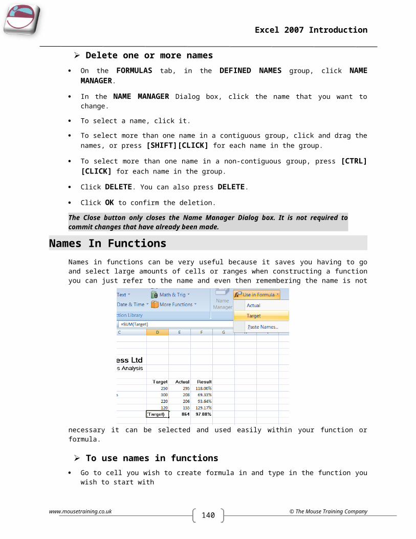
139
Excel 2007 Introduction
ZoomYou can adjust the scale of the on-screen display with the Zoom command. Excel allows you to specify any percentage between 1 and 100 for viewing on-screen data. If there is a particular range that you need to make visible on one screen without scrolling, you can use the Fit selection option.
To zoom screen display:Mouse
In the bottom right hand corner of the screen click on the PLUS or MINUS buttons to zoom in or out of your spreadsheet
OR
Click on the PERCENTAGE button on the bottom right hand corner of your screen and a dialog box will open.
EITHER
Choose a PERCENTAGE from the dialog box
Click OK to apply the zoom and close the dialog.
OR
Highlight the PERCENTAGE figure currently displaying in the CUSTOM Zoom text box and type the figure you want to use.
Click OK to apply the zoom and close the dialog.
© The Mouse Training Company www.mousetraining.co.uk

139
Excel 2007 Introduction
SECTION 11 SORTING & SUBTOTALLING DATA
LISTSExcel’s tabular layout makes it an ideal tool to use for managing lists of data. There are many commands that you can use to manipulate list data, which are described in this section, however, before discussing those, it is worth reviewing the best way to lay out a list in Excel.
DoMAKE THE FIRST ROW OF YOUR LIST THE COLUMN HEADINGS THAT DESCRIBE THE DATA.
Do NotUSE AMBIGUOUS WORDS AS COLUMN HEADINGS (E.G. SUM, SUBTOTAL) AS EXCEL MAY CONFUSE THEM WITH FUNCTIONS OR NAMES THAT YOU HAVE DEFINED.
USE PUNCTUATION IN COLUMN HEADINGS.
LEAVE A GAP BETWEEN THE COLUMN HEADINGS AND THE FIRST ROW OF DATA.
LEAVE BLANK ROWS BETWEEN LIST DATA.
SORTING LIST DATAWhere you have lists with lots of columns and rows, you may need to sort by more than one column. For example the list of orders below has been sorted by customer, within the customer grouping, you may want to sort by Product and then by Salesperson.
Quick Sort
To use a quick sortMouse
Click in the column you wish to sort by
DO NOT HIGHLIGHT ANY DATA
Go to the DATA ribbon and the SORT & FILTER group.
Click on the QUICK SORT buttons ascending or descending
Data should now be sorted
© The Mouse Training Company www.mousetraining.co.uk
Sort tools on the DATA ribbon

140
Excel 2007 Introduction
Multi Level Sort
To sort using the Sort dialog:
Mouse Click in the middle of the list you want to sort.
Go to the DATA ribbon and the SORT & FILTER group. And click on the SORT button
Excel recognises the column headings from your list and allows you to pick them from drop-down list boxes in the dialog.
Choose the column you wish to sort by from the drop down box in the column section
If you have various formats on your cells you can sort on more than just the value click on drop down arrow to see further options
Set ASCENDING or DESCENDING order for the sort by clicking the relevant option.
Click on ADD LEVEL, level will be added to the main area
Repeat previous procedure to add more levels of sort
If you wish to change the order of sort. Select the level you wish to change and click on the movement arrows to move level up or down
To remove a level select it and click on the delete level button it will be removed
Click OK to perform the sort.
www.mousetraining.co.uk © The Mouse Training Company

139
Excel 2007 Introduction
SUBTOTALSExcel can automatically add subtotals to a list of data. Your subtotals can sum numeric data or find highest and lowest values and averages. You can also count the number of rows in a group.
Organising The List For SubtotalsWhen you issue the subtotals command, Excel will need to know where to add the subtotals in. In the example below, if you wanted to see subtotals for the revenue generated per product, you would first need to sort the list into Product order. Similarly, if you wanted to see how much each salesperson had sold; you would sort the list by Salesperson before adding the subtotals in.
To add subtotals to a list:Mouse
Once you have sorted the list, choose SUBTOTALS from the OUTLINE group on the DATA ribbon. The following dialog box will appear:
Click the drop-down list arrow to the right of the 'at each change in' box to display your column headings. Pick the heading according to which column you have used to group the data.
Click the drop-down list arrow to the right of the Use function box to display a list of functions you can use to summarise data in your list. Click the function that you want.
Use the scroll arrows in the Add subtotal to list to set which columns you want to add the subtotals to. Check the box next to the column to subtotal. You can add subtotals to more than one column.
Set options for the new subtotals using the check boxes at the bottom of the dialog.
If you want each subtotalled group on a separate page, check Page Break between groups.
© The Mouse Training Company www.mousetraining.co.uk

140
Excel 2007 Introduction
Summary below detail adds subtotals and an overall total BELOW the groups of data rather than above.
Replace current subtotals ensures that the new subtotals overwrite any existing ones.
Click OK to apply the subtotals.
Example:
To insert the subtotals shown above:- Sort the list by PRODUCT. Choose DATA ribbon, SUBTOTALS.
At each change in PRODUCT, Use function SUM, Add subtotal to TOTAL
www.mousetraining.co.uk © The Mouse Training Company

139
Excel 2007 Introduction
Summarising A Subtotalled ListOnce you have added subtotals to a list, Excel gives you tools for collapsing the list so that you only see the grand total or subtotals. The outline symbols that appear to the left of the row numbers allow you to hide and show detail rows as needed.
To hide detail for a group:Mouse
Click the minus symbol that appears to the left of the row number where the grand/subtotal sits. All bracketed rows will be hidden.
You can see where the hidden rows are because the outline symbol displays a plus sign.
To show detail for a group:Mouse
Click the plus symbol that appears to the left of the row number where the grand total/subtotal sits. All hidden rows will reappear.
Show And Hide By LevelWhen you add subtotals to a list, Excel gives you an overall total and subtotals per groups of sorted data. In the outline, Excel numbers these levels 1 for the grand total, 2 for the subtotals and 3 for the detail.
The numbers appear above the outline symbols and can be used to collapse and expand the rows by level.
To show only an overall total:Mouse
Click the button marked 1 above the outline symbols. To show only totals:
© The Mouse Training Company www.mousetraining.co.uk
Outline symbol
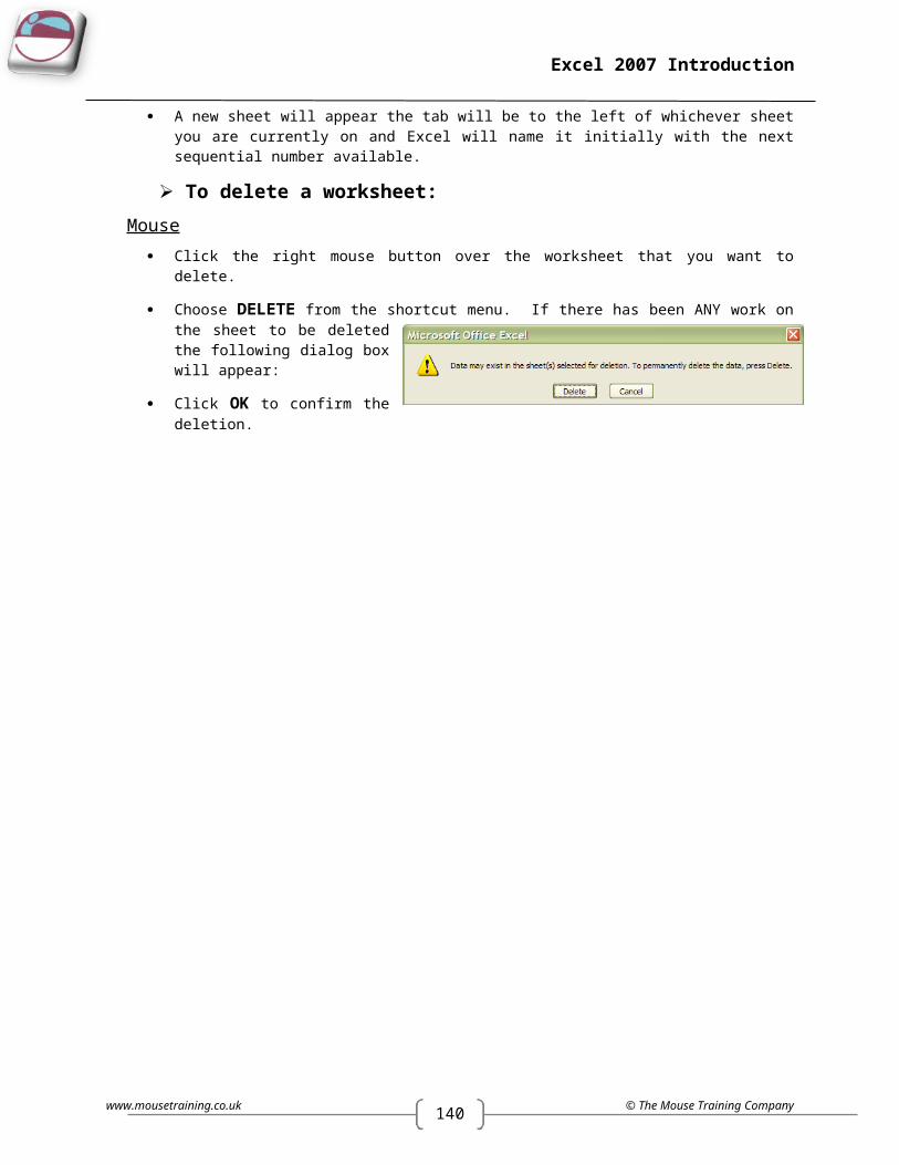
140
Excel 2007 Introduction
Mouse
Click the button marked 2 above the outline symbols.
To show all:Mouse
Click the button marked 3 above the outline symbols.
Remove SubtotalsIf you want to remove subtotals from a list, you can use the Remove subtotals command.
To remove subtotals:Mouse
Click in the list with the subtotals
Choose subtotals from the Data ribbon. From the resulting dialog box, click the REMOVE ALL button. Any totals and outlines will disappear.
www.mousetraining.co.uk © The Mouse Training Company

139
Excel 2007 Introduction
SECTION 12 CUSTOMISING EXCEL
SET EXCEL OPTIONS
OPTIONS ARE SET VERY DIFFERENTLY IN EXCEL 2007
Click the MICROSOFT OFFICE BUTTON, Click the EXCEL OPTIONS button to open the dialog box above
PopularThis sheet allows you to turn off the mini toolbar that appears whenever you right click on a cell or range plus other basic options
You may put in a different username which by default is the logon for windows
Clicking the language settings button allows the setting of the default language not just for excel but for all the office programmes
You may change the deault number of sheets from three to whatever you wish the limitations of excel will be in the next chapter
Editing custom lists for various usages such as drag fill, series and sorting can be done from this sheet
You may even change the colour scheme for excel windows (not dialog boxes)
© The Mouse Training Company www.mousetraining.co.uk
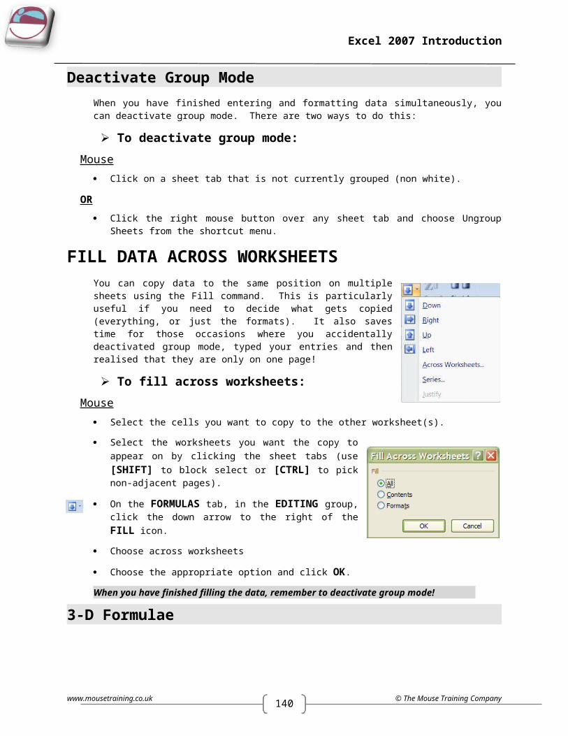
140
Excel 2007 Introduction
Formulas SheetThis sheet allows the setting of options that changes the way excel will calculate your sheets and workbook
ProofingIt is here on the Proofing sheet that the spell-check and grammar options are set for excel.
It also has the options for the autoformatting and autocorrection of entered text
www.mousetraining.co.uk © The Mouse Training Company

139
Excel 2007 Introduction
SaveSAVE is an important sheet since excel 2007 saves in a completely different file format this sheet gives global options on what FILETYPE to save the file as and where to save files by default.This sheet also has the AUTORECOVER options for where and how your files will be AUTOSAVED should windows crash. This saves your work regularly and automatically and should recover work should the worst happen.
ResourcesThis sheet is useful to get updates for office (you do need to be online) and to run the office diagnostics if you encounter errors with the way office works (you will need your original installation disc)
© The Mouse Training Company www.mousetraining.co.uk
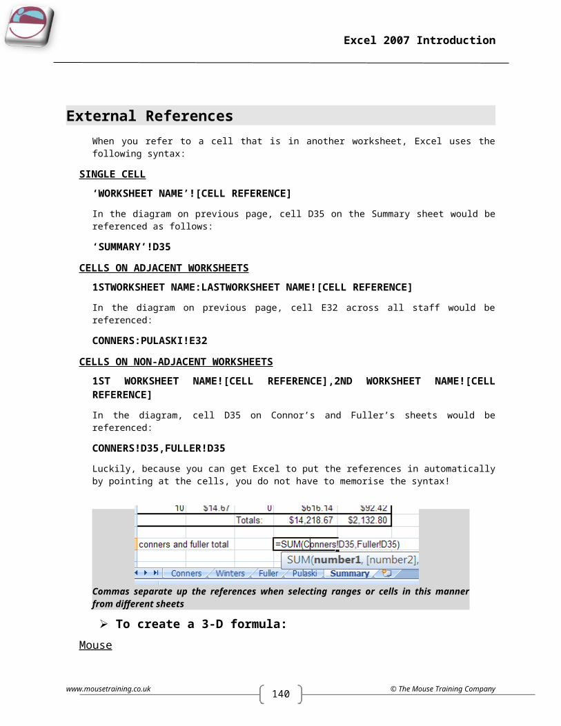
140
Excel 2007 Introduction
ADVANCED OPTIONS
These are all the options on the advanced sheet there are to many to go into but should be useful for reference
www.mousetraining.co.uk © The Mouse Training Company
139
Excel 2007 Introduction
Customise Quick Access ToolbarThis is the location where you are able to customise the quick access toolbar (above the OFFICE BUTTON) and add your most often used buttons to it.
To customise quick access toolbar From the drop down arrow on the top left on the box you may choose which group of commands you
may wish to see.
Select the buttons on the left and click on the add button in the middle to move them to the toolbar.
If you make a mistake then select the button on the right and click remove.
Once all the buttons you want are on the right hand side click ok to finalise your choices and apply them.
You may click on rest at any time to return to the default quick access toolbar
© The Mouse Training Company www.mousetraining.co.uk
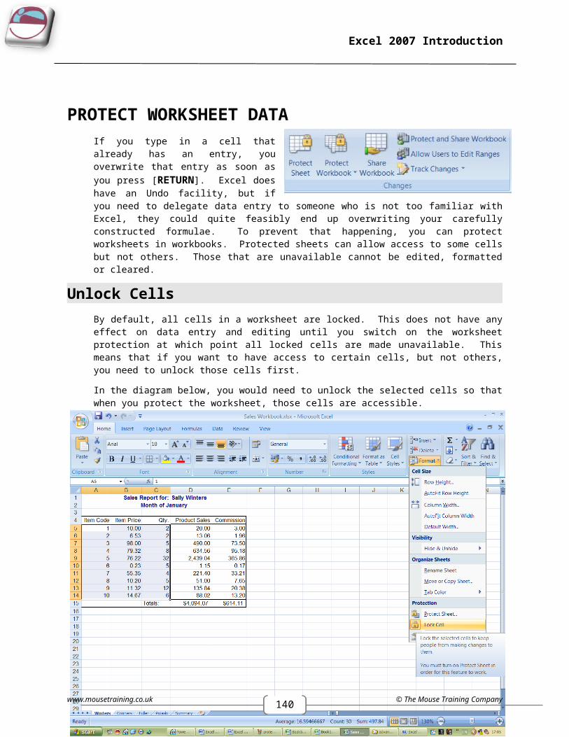
140
Excel 2007 Introduction
EXCEL 2007 SPECIFICATIONS AND LIMITS Worksheet and workbook specifications and limits
Feature Maximum limitOpen workbooks Limited by available memory and system
resourcesWorksheet size 1,048,576 rows by 16,384 columnsColumn width 255 charactersRow height 409 pointsPage breaks 1,026 horizontal and verticalTotal number of characters that a cell can contain 32,767 charactersCharacters in a header or footer 255Sheets in a workbook Limited by available memory (default is 3
sheets)Colours in a workbook 16 million colours (32 bit with full access
to 24 bit colour spectrum)Named views (view: A set of display and print settings that you can name and apply to a workbook. You can create more than one view of the same workbook without saving separate copies of the workbook.) in a workbook
Limited by available memory
Unique cell formats/cell styles 64,000Fill styles 32Line weight and styles 16Unique font types 1,024 global fonts available for use; 512
per workbookNumber formats in a workbook Between 200 and 250, depending on the
language version of Excel that you have installed
Names in a workbook Limited by available memoryWindows in a workbook Limited by available memoryPanes in a window 4Linked sheets Limited by available memoryScenarios (scenario: A named set of input values that you can substitute in a worksheet model.)
Limited by available memory; a summary report shows only the first 251 scenarios
Changing cells in a scenario 32Adjustable cells in Solver 200Custom functions Limited by available memoryZoom range 10 percent to 400 percentReports Limited by available memorySort references 64 in a single sort; unlimited when using
sequential sortsUndo levels 100Fields in a data form 32Workbook parameters 255 parameters per workbookFilter drop-down lists 10,000
Calculation specifications and limitsFeature Maximum limitNumber precision 15 digitsLargest number allowed to be typed into a cell 9.99999999999999E307Largest allowed positive number 1.79769313486231E308Smallest allowed negative number -2.2251E-308Smallest allowed positive number 2.229E-308
www.mousetraining.co.uk © The Mouse Training Company

139
Excel 2007 Introduction
Largest allowed negative number -1E-307Length of formula contents 8,192 charactersInternal length of formula 16,384 bytesIterations 32,767Worksheet arrays Limited by available memorySelected ranges 2,048Arguments in a function 255Nested levels of functions 64User defined function categories 255Number of available worksheet functions 341Size of the operand stack 1,024Cross-worksheet dependency 64,000 worksheets that can refer to other
sheetsCross-worksheet array formula dependency Limited by available memoryArea dependency Limited by available memoryArea dependency per worksheet Limited by available memoryDependency on a single cell 4 billion formulas that can depend on a
single cellLinked cell content length from closed workbooks 32,767Earliest date allowed for calculation January 1, 1900 (January 1, 1904, if 1904
date system is used)Latest date allowed for calculation December 31, 9999Largest amount of time that can be entered 9999:59:59
Charting specifications and limitsFeature Maximum limitCharts linked to a worksheet Limited by available memory Worksheets referred to by a chart 255Data series(Related data points that are plotted in a chart. Each data series in a chart has a unique colour or pattern and is represented in the chart legend. You can plot one or more data series in a chart. Pie charts have only one data series.) in one chart
255
Data points (Individual values that are plotted in a chart. Related data points make up a data series. Data points are represented by bars, columns, lines, slices, dots, and other shapes. These shapes are called data markers.) in a data series for 2-D charts
32,000
Data points in a data series for 3-D charts 4,000Data points for all data series in one chart 256,000
PivotTable and PivotChart report specifications and limitsFeature Maximum limitPivotTable reports (An interactive, cross tabulated Excel report that summarizes and analyzes data, such as database records, from various sources, including ones that are external to Excel.) on a sheet
Limited by available memory
Unique items per field 1,048,576Row (A field that's assigned a row orientation in a PivotTable report. Items associated with a row field are displayed as row labels.) or column fields(A field that's assigned a column orientation in a PivotTable report. Items associated with a column field are displayed as column labels.) in a PivotTable report
Limited by available memory
Report filters in a PivotTable report 256 (may be limited by available memory)
Value fields in a PivotTable report 256Calculated item (An item within a PivotTable field or PivotChart field that uses a Limited by available memory
© The Mouse Training Company www.mousetraining.co.uk
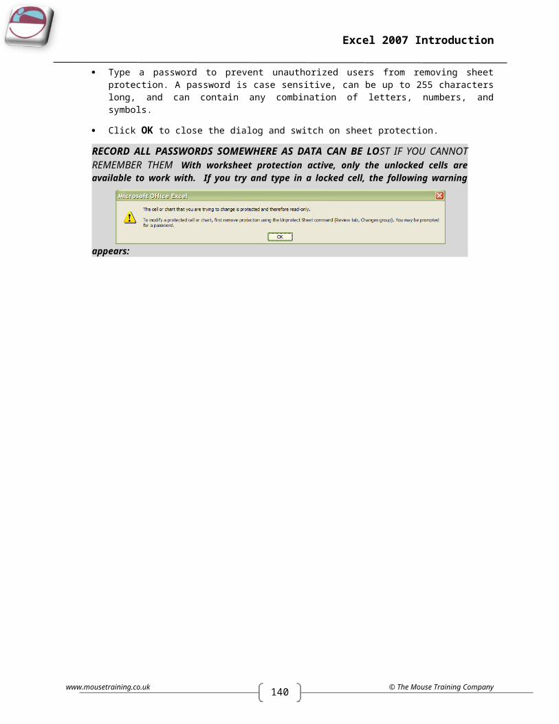
140
Excel 2007 Introduction
formula you create. Calculated items can perform calculations by using the contents of other items within the same field of the PivotTable report or PivotChart report.) formulas in a PivotTable reportReport filters in a PivotChart report(A chart that provides interactive analysis of data, like a PivotTable report. You can change views of data, see different levels of detail or reorganize the chart layout by dragging fields and by showing or hiding items in fields.)
256 (may be limited by available memory)
Value fields in a PivotChart report 256Calculated item formulas in a PivotChart report Limited by available memoryLength of the MDX name for a PivotTable item 32,767Length for a relational PivotTable string 32,767
Shared workbook specifications and limitsFeature Maximum limitUsers who can open and share a shared workbook (shared workbook: A workbook set up to allow multiple users on a network to view and make changes at the same time. Each user who saves the workbook sees the changes made by other users.) at the same time
256
Personal views (view: A set of display and print settings that you can name and apply to a workbook. You can create more than one view of the same workbook without saving separate copies of the workbook.) in a shared workbook
Limited by available memory
Days that change history (In a shared workbook, information that is maintained about changes made in past editing sessions. The information includes the name of the person who made each change, when the change was made, and what data was changed.) is maintained
32,767 (default is 30 days)
Workbooks that can be merged at one time Limited by available memoryCells that can be highlighted in a shared workbook 32,767Colours used to identify changes made by different users when change highlighting is turned on
32 (each user is identified by a separate colour; changes made by the current user are highlighted with navy blue)
www.mousetraining.co.uk © The Mouse Training Company