The Murchison Widefield Array 21 cmPower Spectrum Analysis Methodology

The Harvard community has made thisarticle openly available. Please share howthis access benefits you. Your story matters

Citation Jacobs, Daniel C., B. J. Hazelton, C. M. Trott, Joshua S.Dillon, B. Pindor, I. S. Sullivan, J. C. Pober, et al. 2016. “TheMurchison Widefield Array 21 cm Power Spectrum AnalysisMethodology.” The Astrophysical Journal 825 (2) (July 11): 114.doi:10.3847/0004-637x/825/2/114.

Published Version 10.3847/0004-637x/825/2/114

Citable link http://nrs.harvard.edu/urn-3:HUL.InstRepos:32751005

Terms of Use This article was downloaded from Harvard University’s DASHrepository, and is made available under the terms and conditionsapplicable to Open Access Policy Articles, as set forth at http://nrs.harvard.edu/urn-3:HUL.InstRepos:dash.current.terms-of-use#OAP

Draft version May 24, 2016Preprint typeset using LATEX style emulateapj v. 01/23/15

THE MURCHISON WIDEFIELD ARRAY 21 CM POWER SPECTRUM ANALYSIS METHODOLOGY

Daniel C. Jacobs1,2, B. J. Hazelton3,4, C. M. Trott5,6, Joshua S. Dillon7, B. Pindor5,8, I. S. Sullivan3,J. C. Pober9, N. Barry3, A. P. Beardsley1,3, G. Bernardi10,11,12, Judd D. Bowman1, F. Briggs5,13,

R. J. Cappallo14, P. Carroll3, B. E. Corey14, A. de Oliveira-Costa7, D. Emrich6, A. Ewall-Wice7, L. Feng7,B. M. Gaensler15,5,16, R. Goeke7, L. J. Greenhill12, J. N. Hewitt7, N. Hurley-Walker6, M. Johnston-Hollitt17,

D. L. Kaplan18,3, J. C. Kasper19,12, HS Kim5,8, E. Kratzenberg14, E. Lenc5,16, J. Line5,8, A. Loeb12,C. J. Lonsdale14, M. J. Lynch6, B. McKinley5,8, S. R. McWhirter14, D. A. Mitchell20,5, M. F. Morales3,E. Morgan7, A. R. Neben7, N. Thyagarajan1, D. Oberoi21, A. R. Offringa5,22, S. M. Ord5,6, S. Paul23,

T. Prabu23, P. Procopio5,8, J. Riding5,8, A. E. E. Rogers14, A. Roshi24, N. Udaya Shankar23, Shiv K. Sethi23,K. S. Srivani23, R. Subrahmanyan5,23, M. Tegmark7, S. J. Tingay5,6, M. Waterson13,6, R. B. Wayth5,6,

R. L. Webster5,8, A. R. Whitney14, A. Williams6, C. L. Williams7, C. Wu25,3, J. S. B. Wyithe5,8

Draft version May 24, 2016

ABSTRACT

We present the 21 cm power spectrum analysis approach of the Murchison Widefield Array Epoch ofReionization project. In this paper, we compare the outputs of multiple pipelines for the purpose ofvalidating statistical limits cosmological hydrogen at redshifts between 6 and 12. Multiple, indepen-dent, data calibration and reduction pipelines are used to make power spectrum limits on a fiducialnight of data. Comparing the outputs of imaging and power spectrum stages highlights differencesin calibration, foreground subtraction and power spectrum calculation. The power spectra found us-ing these different methods span a space defined by the various tradeoffs between speed, accuracy,and systematic control. Lessons learned from comparing the pipelines range from the algorithmic tothe prosaically mundane; all demonstrate the many pitfalls of neglecting reproducibility. We brieflydiscuss the way these different methods attempt to handle the question of evaluating a significantdetection in the presence of foregrounds.Keywords: cosmology: dark ages, reionization, first stars — methods: data analysis — techniques:

interferometric

1 Arizona State University, School of Earth and Space Explo-ration, Tempe, AZ 85287, USA

2 e-mail: daniel.c.jacobs@asu.edu3 University of Washington, Department of Physics, Seattle,

WA 98195, USA4 University of Washington, eScience Institute, Seattle, WA

98195, USA5 ARC Centre of Excellence for All-sky Astrophysics (CAAS-

TRO)6 International Centre for Radio Astronomy Research, Curtin

University, Perth, WA 6845, Australia7 MIT Kavli Institute for Astrophysics and Space Research,

Cambridge, MA 02139, USA8 The University of Melbourne, School of Physics, Parkville,

VIC 3010, Australia9 Brown University, Department of Physics, Providence, RI

02912, USA10 Department of Physics and Electronics, Rhodes University,

Grahamstown 6140, South Africa11 Square Kilometre Array South Africa (SKA SA), Park

Road, Pinelands 7405, South Africa12 Harvard-Smithsonian Center for Astrophysics, Cambridge,

MA 02138, USA13 Australian National University, Research School of Astron-

omy and Astrophysics, Canberra, ACT 2611, Australia14 MIT Haystack Observatory, Westford, MA 01886, USA15 Dunlap Institute for Astronomy and Astrophysics, Univer-

sity of Toronto, ON M5S 3H4, Canada16 The University of Sydney, Sydney Institute for Astronomy,

School of Physics, NSW 2006, Australia17 Victoria University of Wellington, School of Chemical &

Physical Sciences, Wellington 6140, New Zealand18 University of Wisconsin–Milwaukee, Department of

Physics, Milwaukee, WI 53201, USA19 University of Michigan, Department of Atmospheric,

Oceanic and Space Sciences, Ann Arbor, MI 48109, USA20 CSIRO Astronomy and Space Science (CASS), PO Box 76,

Epping, NSW 1710, Australia

21 National Centre for Radio Astrophysics, Tata Institute forFundamental Research, Pune 411007, India

22 Netherlands Institute for Radio Astronomy (ASTRON),PO Box 2, 7990 AA Dwingeloo, The Netherlands

23 Raman Research Institute, Bangalore 560080, India24 National Radio Astronomy Observatory, Charlottesville

and Greenbank, USA25 International Centre for Radio Astronomy Research,

University of Western Australia, Crawley, WA 6009, Australia

arX

iv:1

605.

0697

8v1

[as

tro-

ph.I

M]

23

May

201

6

2 D. Jacobs

1. INTRODUCTION

Study of primordial hydrogen in the early universe via21 cm radiation has been forecast to provide a wealth ofastrophysical and cosmological information. Hydrogenis the principal product of big bang nucleosynthesis andis neutral over cosmic time from recombination until re-ionized by the first batch of UV emitters. While neutralit is visible in the 21 cm radio line, which is both op-tically thin and spectrally narrow, making possible fulltomographic reconstruction of a very large fraction of thecosmological volume. Reviews of 21 cm cosmology, astro-physics and observing can be found in Morales & Wyithe(2010); Furlanetto et al. (2006); Pritchard & Loeb (2012);Zaroubi (2013).

Direct detection of HI during the Epoch of Reioniza-tion (cosmological redshifts 5 < z < 13) is currently thegoal of several new radio arrays. The LOw FrequencyARray (LOFAR; Yatawatta et al. 2013), the Donald C.Backer Precision Array for Probing the Epoch of Reion-ization (PAPER; Parsons et al. 2014) and the MurchisonWidefield Array (MWA; Tingay et al. (2013); Bowmanet al. (2013)) are all currently conducting long observingcampaigns.

The analysis of the resulting data presents several chal-lenges. The signal is faint; initial detection is beingsought in the power spectrum with thousands of hoursof integration (accumulated over several years) requiredto make a statistical detection, most commonly in thepower spectrum. This faint spectral line signal sits atop acontinuum foreground four orders of magnitude brighter(Santos & Cooray 2006; Bowman et al. 2009; Pober et al.2013). At the same time, the instruments are fully cor-related phased arrays with wide fields of view that strainthe conventional mathematical approximations of radioastronomy practice (e.g. Thompson et al. (2007)). Themethods used to arrive at a well-calibrated, foreground-free estimation of the power spectrum are all under de-velopment; both the algorithms as well as their imple-mentation.New tools for Power Spectra in the Presence

of Foregrounds

The path from observation to power spectrum can beroughly divided into two parts: removal of foregroundsand estimation of power spectrum. Methods for esti-mating the power spectrum, particularly those whichminimize the effects of foregrounds, have been stud-ied and implemented by Morales et al. (2006a); Jelicet al. (2008); Harker et al. (2009); Morales et al. (2012);Liu & Tegmark (2011); Trott et al. (2012); Chapmanet al. (2012, 2013); Dillon et al. (2013, 2014); Liu et al.(2014a,b). Common elements include using knowledgeabout the instrument and foregrounds to minimize andisolate foreground contamination, applying the quadraticestimator formalism to achieve favorable error proper-ties, and studies of effects related to including the spec-tral dimension in the Fourier transform; i.e. translatingtwo dimensional power spectrum techniques from CMBapplications into three dimensional which also take aFourier transform along the spectral/line of sight dimen-sion. One significant problem studied has been mini-mizing the impact of any residual foregrounds by down-weighting or minimizing correlation with contaminated

band powers. In this paper we compare power spectracalculated using a range of methods.

The various dimensions of the 3D power spectrumspace are used frequently throughout this paper. Trans-verse modes k⊥ are directly sampled by baselines oflength |u|1 while line of sight modes k‖ are measured as ηmodes which are the Fourier dual to frequency. Note alsothat for shorter baselines there is an approximate equiv-alence between η and the geometric delay of wavefrontsmoving across the array. Here we follow the conventionsof Furlanetto et al. (2006) relating the measured modesto their cosmological counterparts using a ΛCDM cos-mology with H0 = 100h kms−1Mpc−1,ΩM = 0.27,Ωk =0,Ωk = 0.73 (Hinshaw et al. 2013).

The 21 cm power spectrum increases steeply with de-creasing wave number making it desirable to remove fore-grounds on the largest spatial and spectral scales possi-ble. These foregrounds, by virtue of the correlation func-tion of the interferometer, have a chromatic response inthe instrument which has a spectral period that increaseswith baseline length and distance from phase center. Ina 2D power spectrum spanning line of sight and angularmodes this produces a wedge-shaped feature which hasbeen much discussed in the literature Datta et al. (2010);Vedantham et al. (2012a); Parsons et al. (2012); Poberet al. (2013); Morales et al. (2012); Liu et al. (2014a,b);Dillon et al. (2015); Trott et al. (2012); Thyagarajanet al. (2015a). Sources far from the phase center—nearthe Earth’s horizon—show up in the topmost part of thewedge and thus contribute most strongly to nominallyuncontaminated modes.

Recently, two sorts of foreground removal have beensuggested: methods which exploit detailed knowledgeof foregrounds and those which are relatively agnosticabout the individual foreground sources. Among the lat-ter, several authors have described methods for fittingand removing smooth spectrum foregrounds from imagecubes (Morales et al. 2006b; Bowman et al. 2009; Liuet al. 2009; Liu & Tegmark 2011; Chapman et al. 2012;Chapman et al. 2013; Dillon et al. 2013; Yatawatta et al.2013). These methods have been demonstrated to ro-bustly remove foregrounds near the field center but areless effective for sources far from the central lobe of theprimary beam, i.e. in the wedge (Thyagarajan et al.2015a,b; Pober et al. 2016). A second class of agnosticmethods is the delay/fringe-rate filtering approach (Par-sons et al. 2012; Liu et al. 2014a,b), which has been ap-plied to data from PAPER (Parsons et al. 2014; Ali et al.2015; Jacobs et al. 2015). Applying time and frequencydomain filters to the time ordered data, this techniqueuses a small amount of knowledge about the instrumentto filter out the wedge at high dynamic range. Thismethod removes smooth spectrum foregrounds across theentire sky and is comparatively robust in the face of un-certainty about the instrument at the cost of losing somesensitivity.

Meanwhile, full forward modeling and subtraction ofa sky model such as that implemented for LOFAR (seee.g. Jelic et al. (2008); Yatawatta et al. (2013)) has thegoal of directly subtracting the sources responsible forthe wedge and accessing the shortest, brightest 21 cm

1Note that the mapping between k⊥ and baseline vector u isonly strictly true in the small field of view limit.

MWA Power Spectra 3

wavemodes. To this requires a much higher fidelity modelof the instrument and foregrounds across the entire sky,horizon to horizon (Thyagarajan et al. 2015a).

The MWA foreground removal approach leverages thearray’s optimization for imaging to directly subtractknown foregrounds in addition to the full range oftreatments of residual foregrounds, including foregroundavoidance and foreground suppression. If successful, di-rect subtraction opens the most sensitive power spec-trum modes, substantially improving the ability of earlymeasurements to distinguish between reionization mod-els (Beardsley et al. 2013; Pober et al. 2014). Recentwork towards the goal of foreground subtraction includesbetter algorithmic handling of wide field imaging effects(Tasse et al. 2012; Bhatnagar et al. 2013; Sullivan et al.2012; Ord et al. 2010; Offringa et al. 2014), and contin-ually improving catalogs of sky emission (de Oliveira-Costa et al. 2008; Jacobs et al. 2011; Jacobs et al.2013; Hurley-Walker et al. 2014). Ongoing operation ofthe first generation low frequency arrays—LOFAR, PA-PER and MWA are all in their third or fourth year ofoperation—continues to push the refinement of instru-mental models (e.g. the work of Neben et al. (2015) inmapping the primary beam with satellites) and improvethe accuracy of model subtraction. At the same time,more complete surveys of foregrounds are currently underway. These include the MWA GLEAM1 survey (Waythet al. 2015), GMRT TGSS(Intema et al. 2016) and theLOFAR MSSS2 (Heald et al. 2015)..

In turn, efforts with these currently operational experi-ments are having a major influence on how future, larger,EoR experiments will be designed and conducted. Pri-mary among these future experiments will be programsusing the low frequency Square Kilometre Array (Koop-mans et al. (2014)) and the Hydrogen Epoch of Reioniza-tion Array (HERA; Pober et al. 2014). Specifically, theMWA is one of three official precursor telescopes for theSKA and the only one of the three fully operational forscience. The low frequency SKA will be located at theMWA site in Western Australia, giving the MWA specialsignificance.

Given the challenges of using newly developed meth-ods to reduce data from a novel instrument to make alow sensitivity detection, it is reasonable to consider thequestion of how one knows one is getting the “right”answer. One option is to generate, as accurately as pos-sible, a detailed simulation of the interferometer outputand then input that to the pipeline under test. Suchforward modeling is an essential tool for checking cor-rect operation of portions of the pipeline; however, themodel will always be an imperfect reflection of reality,leaving open multiple interpretations of any differencesbetween model and data. Forward modeling the instru-ment response is also difficult to divorce from the analysispipeline being tested; often the same software doing theanalysis is used to perform the simulations. A second op-tion, and the focus of this paper, is comparison betweenmultiple independent pipelines.

In section 2 we summarize the observing strategyused to collect our data, section 3 explains our multiplepipelines and comparison strategy. In section 4 we show

1GLEAM: GaLactic and Extragalactic All-sky MWA2MSSS: Multi-frequency Snapshot Sky Survey

comparisons of images, diagnostic power spectra, powerspectrum limits, section 5 lists some lessons learned fromthe comparison process and section 6 offers some conclu-sions.

2. OBSERVING

2.1. The MWA

The MWA is an interferometric array of phased ar-ray tiles operating in the 80-300 MHz radio band. Eachtile consists of a 4x4 grid of dual polarization bow-tieshaped dipoles that are used to form a beam on the skywith a full width of 26(λ/2m) at the half power point.Signals from individual antennas are summed by an ana-log delay-line beamformer which can steer the beam insteps of 6.8cos(elevation). The signal is digitized overthe entire bandwidth but only 30.72 MHz are availableat any one time. This 30 MHz of bandwidth is brokeninto 1.28 MHz “coarse” bands by a polyphase filter-bankin the field and sent to the correlator (Ord et al. 2015)where it is further channelized to 40kHz, cross-multipliedand then averaged at 0.5 second intervals. More detailson the design and operation of the MWA can be foundin Lonsdale et al. (2009) and Tingay et al. (2013).

2.2. The 21 cm Observing Program

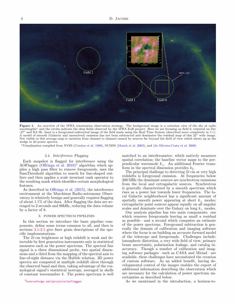
The MWA reionization observing scheme spans two30 MHz tunings, 140-170 MHz (9.2< z <7.5) and 167-196 MHz (7.5< z <6.25) and two primary minimal fore-ground regions (Field 0 at RA 0h,-27and Field 1 at 4h,Dec -27); both transit the zenith at the MWA’s latitudeand are near the south galactic pole. A third pointingtowards Hydra A is also observed; see Figure 1 for anoverview. Here we focus on the low redshift tuning, andthe RA=0h pointing, where the band is chosen for itslower sky temperature and pointing is chosen for its easeof calibration—having fewer bright, resolved sources; seeTable 1 for a listing of observing parameters.

The analysis presented here is on three hours of data,one of 400 nights which have been collected as part of theobserving program; 150 nights are thought to be neces-sary for a detection of typical models (Beardsley et al.2013).

2.3. Data Included Here

During observing, the beam-former was set such thatthe target region repeatedly drifted through the field ofview. With an available beamformer step size of 6.8;each drift was about 30 minutes long. This was donefor a total of 6 pointings in a night, or about 3 hours.The data included here include the two pointings leadingup to the target crossing zenith, the zenith pointing, andthen three more pointings after the transit crossing. Datawere recorded in 112 second units (which we term “snap-shots”) for a total of 96 snapshots. These snapshots arethe basic unit of time on which many operations becomeindependent -eg RFI flagging, calibration and imaging.Though the full set of linear polarization parameters arecorrelated, and Stokes I images and power spectra arethe final product of interest, at this stage of the anal-ysis the instrumental polarizations have been found tobe more instructive; with one exception, only the lineareast-west polarization is examined here. No significantdifferences are seen in the north-south data. The sameset of snapshots is used in every pipeline run.

4 D. Jacobs

Figure 1. An overview of the MWA reionization observation strategy. The background image is a cartesian view of the sky at radiowavelengthsa and the circles indicate the deep fields observed by the MWA EoR project. Here we are focusing on field 0, centered on Dec-27 and RA 0h. Inset is a foreground subtracted image of the field made using the Real Time System (described more completely in 3.1).A model of smooth (Galactic and unresolved) emission has not been subtracted and dominates the residual map of this 22 wide image.Not visible in this average map is variation from channel to channel caused by sources far beyond the field of view which shows up as thewedge in 2d power spectra.aVisualization compiled from NVSS (Condon et al. 1998), SUMSS (Mauch et al. 2003), and (de Oliveira-Costa et al. 2008)

2.4. Interference Flagging

Each snapshot is flagged for interference using theAOFlagger (Offringa et al. 2010)3 algorithm which ap-plies a high pass filter to remove foregrounds, uses theSumThreshold algorithm to search for line-shaped out-liers and then applies a scale invariant rank operator tothe resulting mask which identifies certain morphologicalfeatures.

As described in Offringa et al. (2015), the interferenceenvironment at the Murchison Radio-astronomy Obser-vatory is relatively benign and generally requires flaggingof about 1.1% of the data. After flagging the data are av-eraged to 2 seconds and 80kHz, reducing the data volumeby a factor of 8.

3. POWER SPECTRUM PIPELINES

In this section we introduce the basic pipeline com-ponents, define some terms common to all, and then insections 3.1-3.5 give finer grain descriptions of the spe-cific implementations.

The 21 cm brightness at high redshift is weak and de-tectable by first generation instruments only in statisticalmeasures such as the power spectrum. The spectral linesignal is a three dimensional probe, two spatial dimen-sions and a third from the mapping of the spectral axis toline-of-sight distance via the Hubble relation. 3D powerspectra are computed at multiple redshift slices throughthe observed band and then, taking advantage of the cos-mological signal’s statistical isotropy, averaged in shellsof constant wavenumber k. The power spectrum is well

3sourceforge.net/projects/aoflagger

matched to an interferometer, which natively measuresspatial correlation; the baseline vector maps to the per-pendicular wavemode k⊥. An additional Fourier trans-form in the spectral dimension provides k‖.

The principal challenge to detecting 21 cm at very highredshifts is foreground emission. At frequencies below200 MHz the dominant sources are synchrotron emissionsfrom the local and extragalactic sources. Synchrotronis generally characterized by a smooth spectrum whichrises as a power law towards lower frequencies. The lo-cal Galactic neighborhood has a significant amount ofspatially smooth power appearing at short k⊥ modes;extragalactic point sources appear equally on all angularscales and dominate over the Galaxy on long k⊥ modes.

Our analysis pipeline has two main components: onewhich removes foregrounds–leaving as small a residualas possible—and a second which computes an estimateof the power spectrum. Foreground subtraction is gen-erally the domain of calibration and imaging softwarewhere the focus is on building an accurate forward modelof the telescope and foregrounds. Challenges include:ionospheric distortion, a very wide field of view, primarybeam uncertainty, polarization leakage, and catalog in-accuracy. Though a number of calibration and imag-ing software packages—such as CASA and Miriad—areavailable, these challenges have necessitated the creationof custom software. As an added benefit, having de-velopmental control of the imager enables the export ofadditional information describing the observation whichare necessary for the calculation of power spectrum un-certainties as described below.

As we mentioned in the introduction, a horizon-to-

MWA Power Spectra 5

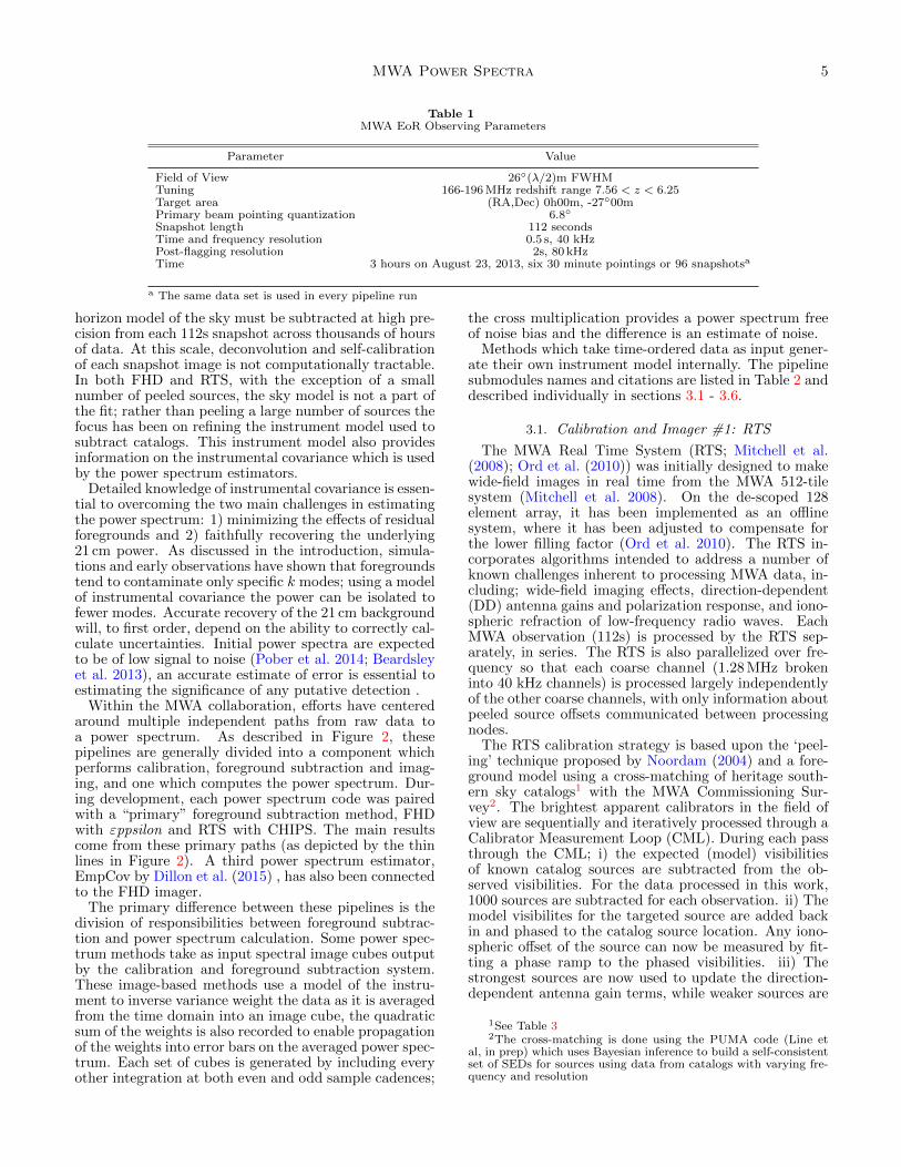
Table 1MWA EoR Observing Parameters

Parameter Value

Field of View 26(λ/2)m FWHMTuning 166-196 MHz redshift range 7.56 < z < 6.25Target area (RA,Dec) 0h00m, -2700mPrimary beam pointing quantization 6.8

Snapshot length 112 secondsTime and frequency resolution 0.5 s, 40 kHzPost-flagging resolution 2s, 80 kHzTime 3 hours on August 23, 2013, six 30 minute pointings or 96 snapshotsa

a The same data set is used in every pipeline run

horizon model of the sky must be subtracted at high pre-cision from each 112s snapshot across thousands of hoursof data. At this scale, deconvolution and self-calibrationof each snapshot image is not computationally tractable.In both FHD and RTS, with the exception of a smallnumber of peeled sources, the sky model is not a part ofthe fit; rather than peeling a large number of sources thefocus has been on refining the instrument model used tosubtract catalogs. This instrument model also providesinformation on the instrumental covariance which is usedby the power spectrum estimators.

Detailed knowledge of instrumental covariance is essen-tial to overcoming the two main challenges in estimatingthe power spectrum: 1) minimizing the effects of residualforegrounds and 2) faithfully recovering the underlying21 cm power. As discussed in the introduction, simula-tions and early observations have shown that foregroundstend to contaminate only specific k modes; using a modelof instrumental covariance the power can be isolated tofewer modes. Accurate recovery of the 21 cm backgroundwill, to first order, depend on the ability to correctly cal-culate uncertainties. Initial power spectra are expectedto be of low signal to noise (Pober et al. 2014; Beardsleyet al. 2013), an accurate estimate of error is essential toestimating the significance of any putative detection .

Within the MWA collaboration, efforts have centeredaround multiple independent paths from raw data toa power spectrum. As described in Figure 2, thesepipelines are generally divided into a component whichperforms calibration, foreground subtraction and imag-ing, and one which computes the power spectrum. Dur-ing development, each power spectrum code was pairedwith a “primary” foreground subtraction method, FHDwith εppsilon and RTS with CHIPS. The main resultscome from these primary paths (as depicted by the thinlines in Figure 2). A third power spectrum estimator,EmpCov by Dillon et al. (2015) , has also been connectedto the FHD imager.

The primary difference between these pipelines is thedivision of responsibilities between foreground subtrac-tion and power spectrum calculation. Some power spec-trum methods take as input spectral image cubes outputby the calibration and foreground subtraction system.These image-based methods use a model of the instru-ment to inverse variance weight the data as it is averagedfrom the time domain into an image cube, the quadraticsum of the weights is also recorded to enable propagationof the weights into error bars on the averaged power spec-trum. Each set of cubes is generated by including everyother integration at both even and odd sample cadences;

the cross multiplication provides a power spectrum freeof noise bias and the difference is an estimate of noise.

Methods which take time-ordered data as input gener-ate their own instrument model internally. The pipelinesubmodules names and citations are listed in Table 2 anddescribed individually in sections 3.1 - 3.6.

3.1. Calibration and Imager #1: RTS

The MWA Real Time System (RTS; Mitchell et al.(2008); Ord et al. (2010)) was initially designed to makewide-field images in real time from the MWA 512-tilesystem (Mitchell et al. 2008). On the de-scoped 128element array, it has been implemented as an offlinesystem, where it has been adjusted to compensate forthe lower filling factor (Ord et al. 2010). The RTS in-corporates algorithms intended to address a number ofknown challenges inherent to processing MWA data, in-cluding; wide-field imaging effects, direction-dependent(DD) antenna gains and polarization response, and iono-spheric refraction of low-frequency radio waves. EachMWA observation (112s) is processed by the RTS sep-arately, in series. The RTS is also parallelized over fre-quency so that each coarse channel (1.28 MHz brokeninto 40 kHz channels) is processed largely independentlyof the other coarse channels, with only information aboutpeeled source offsets communicated between processingnodes.

The RTS calibration strategy is based upon the ‘peel-ing’ technique proposed by Noordam (2004) and a fore-ground model using a cross-matching of heritage south-ern sky catalogs1 with the MWA Commissioning Sur-vey2. The brightest apparent calibrators in the field ofview are sequentially and iteratively processed through aCalibrator Measurement Loop (CML). During each passthrough the CML; i) the expected (model) visibilitiesof known catalog sources are subtracted from the ob-served visibilities. For the data processed in this work,1000 sources are subtracted for each observation. ii) Themodel visibilites for the targeted source are added backin and phased to the catalog source location. Any iono-spheric offset of the source can now be measured by fit-ting a phase ramp to the phased visibilities. iii) Thestrongest sources are now used to update the direction-dependent antenna gain terms, while weaker sources are

1See Table 32The cross-matching is done using the PUMA code (Line et

al, in prep) which uses Bayesian inference to build a self-consistentset of SEDs for sources using data from catalogs with varying fre-quency and resolution

6 D. Jacobs

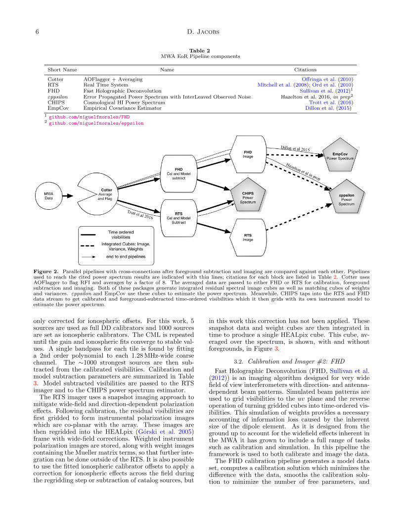
Table 2MWA EoR Pipeline components

Short Name Name Citations

Cotter AOFlagger + Averaging Offringa et al. (2010)RTS Real Time System Mitchell et al. (2008); Ord et al. (2010)FHD Fast Holographic Deconvolution Sullivan et al. (2012)1

εppsilon Error Propagated Power Spectrum with InterLeaved Observed Noise Hazelton et al. 2016, in prep2

CHIPS Cosmological HI Power Spectrum Trott et al. (2016)EmpCov Empirical Covariance Estimator Dillon et al. (2015)

1 github.com/miguelfmorales/FHD2 github.com/miguelfmorales/eppsilon

Figure 2. Parallel pipelines with cross-connections after foreground subtraction and imaging are compared against each other. Pipelinesused to reach the cited power spectrum results are indicated with thin lines; citations for each block are listed in Table 2. Cotter usesAOFlagger to flag RFI and averages by a factor of 8. The averaged data are passed to either FHD or RTS for calibration, foregroundsubtraction and imaging. Both of these packages generate integrated residual spectral image cubes as well as matching cubes of weightsand variances. εppsilon and EmpCov use these cubes to estimate the power spectrum. Meanwhile, CHIPS taps into the RTS and FHDdata stream to get calibrated and foreground-subtracted time-ordered visibilities which it then grids with its own instrument model toestimate the power spectrum.

only corrected for ionospheric offsets. For this work, 5sources are used as full DD calibrators and 1000 sourcesare set as ionospheric calibrators. The CML is repeateduntil the gain and ionospheric fits converge to stable val-ues. A single bandpass for each tile is found by fittinga 2nd order polynomial to each 1.28 MHz-wide coarsechannel. The ∼1000 strongest sources are then sub-tracted from the calibrated visibilities. Calibration andmodel subtraction parameters are summarized in Table3. Model subtracted visibilities are passed to the RTSimager and to the CHIPS power spectrum estimator.

The RTS imager uses a snapshot imaging approach tomitigate wide-field and direction-dependent polarizationeffects. Following calibration, the residual visibilities arefirst gridded to form instrumental polarization imageswhich are co-planar with the array. These images arethen regridded into the HEALpix (Gorski et al. 2005)frame with wide-field corrections. Weighted instrumentpolarization images are stored, along with weight imagescontaining the Mueller matrix terms, so that further inte-gration can be done outside of the RTS. It is also possibleto use the fitted ionospheric calibrator offsets to apply acorrection for ionospheric effects across the field duringthe regridding step or subtraction of catalog sources, but

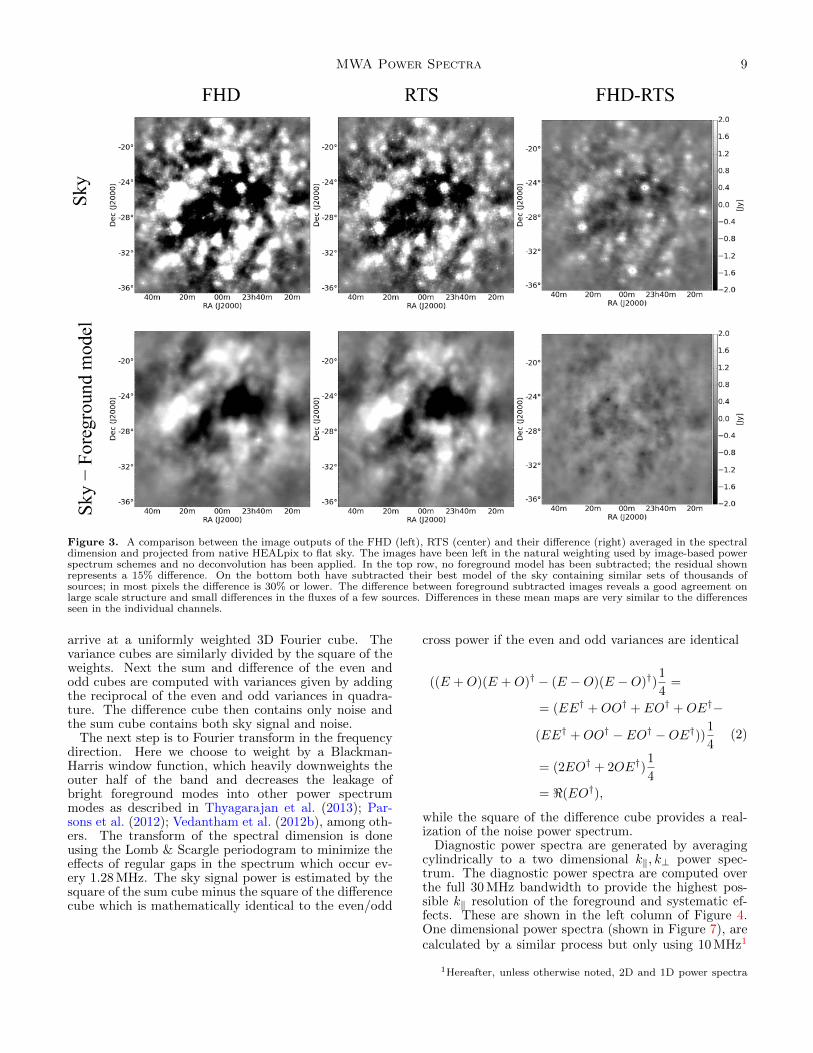
in this work this correction has not been applied. Thesesnapshot data and weight cubes are then integrated intime to produce a single HEALpix cube. This cube, av-eraged over the spectrum, is shown, with and withoutforegrounds, in Figure 3.

3.2. Calibration and Imager #2: FHD

Fast Holographic Deconvolution (FHD, Sullivan et al.(2012)) is an imaging algorithm designed for very widefield of view interferometers with direction- and antenna-dependent beam patterns. Simulated beam patterns areused to grid visibilities to the uv plane and the reverseoperation of turning gridded cubes into time-ordered vis-ibilities. This simulation of weights provides a necessaryaccounting of information loss caused by the inherentsize of the dipole element. As it is designed from theground up to account for the widefield effects inherent inthe MWA it has grown to include a full range of taskssuch as calibration and simulation. In this pipeline theframework is used to both calibrate and image the data.

The FHD calibration pipeline generates a model dataset, computes a calibration solution which minimizes thedifference with the data, smooths the calibration solu-tion to minimize the number of free parameters, and

MWA Power Spectra 7

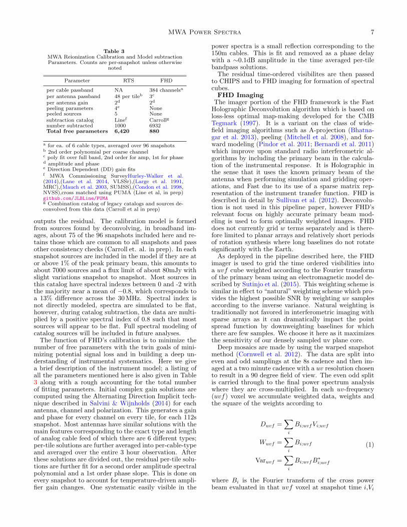
Table 3MWA Reionization Calibration and Model subtractionParameters. Counts are per-snapshot unless otherwise

noted

Parameter RTS FHD

per cable passband NA 384 channelsa

per antenna passband 48 per tileb 3c

per antenna gain 2d 2d

peeling parameters 4e Nonepeeled sources 5 Nonesubtraction catalog Linef Carrollg

number subtracted 1000 6932Total free parameters 6,420 880

a for ea. of 6 cable types, averaged over 96 snapshotsb 2nd order polynomial per coarse channelc poly fit over full band, 2nd order for amp, 1st for phased amplitude and phasee Direction Dependent (DD) gain fitsf MWA Commissioning SurveyHurley-Walker et al.(2014),(Lane et al. 2014, VLSSr),(Large et al. 1991,MRC),(Mauch et al. 2003, SUMSS),(Condon et al. 1998,NVSS),cross matched using PUMA (Line et al, in prep)github.com/JLBLine/PUMAg Combination catalog of legacy catalogs and sources de-convolved from this data (Carroll et al in prep)

outputs the residual. The calibration model is formedfrom sources found by deconvolving, in broadband im-ages, about 75 of the 96 snapshots included here and re-tains those which are common to all snapshots and passother consistency checks (Carroll et. al. in prep). In eachsnapshot sources are included in the model if they are ator above 1% of the peak primary beam, this amounts toabout 7000 sources and a flux limit of about 80mJy withslight variations snapshot to snapshot. Most sources inthis catalog have spectral indexes between 0 and -2 withthe majority near a mean of −0.8, which corresponds toa 13% difference across the 30 MHz. Spectral index isnot directly modeled, spectra are simulated to be flat,however, during catalog subtraction, the data are multi-plied by a positive spectral index of 0.8 such that mostsources will appear to be flat. Full spectral modeling ofcatalog sources will be included in future analyses.

The function of FHD’s calibration is to minimize thenumber of free parameters with the twin goals of mini-mizing potential signal loss and in building a deep un-derstanding of instrumental systematics. Here we givea brief description of the instrument model; a listing ofall the parameters mentioned here is also given in Table3 along with a rough accounting for the total numberof fitting parameters. Initial complex gain solutions arecomputed using the Alternating Direction Implicit tech-nique described in Salvini & Wijnholds (2014) for eachantenna, channel and polarization. This generates a gainand phase for every channel on every tile, for each 112ssnapshot. Most antennas have similar solutions with themain features corresponding to the exact type and lengthof analog cable feed of which there are 6 different types;per-tile solutions are further averaged into per-cable-typeand averaged over the entire 3 hour observation. Afterthese solutions are divided out, the residual per-tile solu-tions are further fit for a second order amplitude spectralpolynomial and a 1st order phase slope. This is done onevery snapshot to account for temperature-driven ampli-fier gain changes. One systematic easily visible in the

power spectra is a small reflection corresponding to the150m cables. This is fit and removed as a phase delaywith a ∼0.1dB amplitude in the time averaged per-tilebandpass solutions.

The residual time-ordered visibilites are then passedto CHIPS and to FHD imaging for formation of spectralcubes.FHD Imaging

The imager portion of the FHD framework is the FastHolographic Deconvolution algorithm which is based onloss-less optimal map-making developed for the CMBTegmark (1997). It is a variant on the class of wide-field imaging algorithms such as A-projection (Bhatna-gar et al. 2013), peeling (Mitchell et al. 2008), and for-ward modeling (Pindor et al. 2011; Bernardi et al. 2011)which improve upon standard radio interferometric al-gorithms by including the primary beam in the calcula-tion of the instrumental response. It is Holographic inthe sense that it uses the known primary beam of theantenna when performing simulation and gridding oper-ations, and Fast due to its use of a sparse matrix rep-resentation of the instrument transfer function. FHD isdescribed in detail by Sullivan et al. (2012). Deconvolu-tion is not used in this pipeline paper, however FHD’srelevant focus on highly accurate primary beam mod-eling is used to form optimally weighted images. FHDdoes not currently grid w terms separately and is there-fore limited to planar arrays and relatively short periodsof rotation synthesis where long baselines do not rotatesignificantly with the Earth.

As deployed in the pipeline described here, the FHDimager is used to grid the time ordered visibilities intoa uvf cube weighted according to the Fourier transformof the primary beam using an electromagnetic model de-scribed by Sutinjo et al. (2015). This weighting scheme issimilar in effect to “natural” weighting scheme which pro-vides the highest possible SNR by weighting uv samplesaccording to the inverse variance. Natural weighting istraditionally not favored in interferometric imaging withsparse arrays as it can dramatically impact the pointspread function by downweighting baselines for whichthere are few samples. We choose it here as it maximizesthe sensitivity of our densely sampled uv plane core.

Deep mosaics are made by using the warped snapshotmethod (Cornwell et al. 2012). The data are split intoeven and odd samplings at the 8s cadence and then im-aged at a two minute cadence with a uv resolution chosento result in a 90 degree field of view. The even odd splitis carried through to the final power spectrum analysiswhere they are cross-multiplied. In each uv-frequency(uvf) voxel we accumulate weighted data, weights andthe square of the weights according to

Duvf =∑i

Bi;uvfVi;uvf

Wuvf =∑i

Bi;uvf

Varuvf =∑i

Bi;uvfB∗i;uvf

(1)

where Bi is the Fourier transform of the cross powerbeam evaluated in that uvf voxel at snapshot time i,Vi

8 D. Jacobs

is visibility at time i1. Essentially D is numerator of themean performed in the mosaicing step with W the nor-malizing denominator of the mean; the same is done forthe error cube Var/W 2.2 The cubes are Fourier trans-formed, corrected for the w projection coordinate warp-ing, and gridded into the HEALpix frame.Mosaicing

The 112 snapshot HEALpix cubes are summed in time,keeping pixels with a beam weight of 1% or more, a cutwhich effectively limits the field of view to ∼20. Theresulting mosaic is handed on to εppsilon (S. 3.4) andEmpCov (S 3.6). This image, averaged over the spec-tral dimension, is shown, with and without foregrounds,in Figure 3. This image retains the full weighting pro-portional to the number of samples in each uvf cell andis therefore very similar to natural weighting. Thoughbeam weighting theoretically gives an optimal inversevariance weighting for each snapshot it does not capturethe change in variance due to changing system temper-ature. The mosaicing as performed here weights eachsnapshot equally, under the assumption that the systemtemperature, which is dominated by the temperature ofthe sky in the direction of the phased array pointing,stays roughly constant through the three hour trackedintegration.

3.3. Comparing Calibration and Imaging Steps

Through the parallel-but-convergent development ofthese imagers have emerged two very similar systems;however, some differences remain in the analysis cap-tured here. The two primary differences are in the treat-ment of calibration and in the subtracted catalogs.

In both pipelines the calibration is a two step process.First, calibration solutions for each channel, and antennaare computed by solving for the least-squares differencewith a model data set. Next, those solutions are fit to amodel of the array; for example fitting a polynomial tothe bandpass. FHD and RTS take different approachesto this step, a fact reflected in the the number of freeparameters in this fit. A smaller number of parame-ters minimizes the possibility of cosmological signal lossor the spurious incorporation of unmodeled foregroundemission in the calibration solutions (Barry et al. 2016);more free parameters can absorb physics missing fromthe instrument model. As tabulated in Table 3 the RTSfits for ∼6,420 free parameters while FHD fits for ∼880.

In practice, some parameters will be averaged overmore than a single night which will further reduce thenumber of free parameters per observation, though hun-dreds to thousands of free parameters is still typical. Thisis a large number but it is considerably smaller than the

1We are not assuming Einstein notation; all sums are writtenexplicitly

2Note that D/W , the cube used to calculate power spectra,represents our best estimate of the power perceived by the instru-ment; an image made from this cube would still be attenuated byone factor of the primary beam. Dividing out by this last factorin the image space would substantially increase the uv correlationlength and invalidate our assumption of uvf diagonality. Becausewe do not divide out by this factor of the beam, we do not formStokes cubes, which are only defined for images with a uniformflux scale. The remaining factor of the primary beam constitutesa volume term in the power spectrum that we account for in thenormalization of the power spectrum using the same conventionsas CHIPS (Trott et al. (2016)).

180 million data points typically recorded in single snap-shot obdservation.

As has been noted, there is nearly an order of mag-nitude difference in the number of free parameters be-tween the two pipelines, which is worth considering. Theprimary difference is in the treatment of the passband.There are a number effects which show up in the pass-band calibration. The edges of the 1.28 MHz bands areknown to be subject to aliasing from adjacent coarsechannels as well as under-sampling when cast to 4bitintegers by the correlator (van Vleck corrections) andso are flagged. This flagging creates a regular samplingfunction which shows up as the characteristic horizontallines in a 2D power spectrum (see section 4.1). Addedto this is a small amount of interference flagging. Addi-tionally, reflections at analog cable junctions show up asadditional spectral ripple corresponding to the length ofthe cables.

The RTS fits for a low order polynomial on every1.28 MHz chunk on every antenna, while FHD averageseach channel over all antennas to get a common pass-band for all and then fits a low order polynomial to getany tile to tile variation. This significantly reduces thenumber of free parameters and the likelihood of signalloss, though leaving open the possibility of additionalun-modeled instrumental effects.

The construction of the foreground subtraction modelis also a point of difference between the two pipelines. Asnoted in Table 3, foreground/calibration models containdifferent numbers of sources which have been derived bydifferent means. The RTS catalog cross-matches multipleheritage southern sky catalogs with the MWA Commis-sioning Survey using the Bayesian cross-matcher PUMA(Line et al in Prep). The FHD subtraction model con-tains sources found in a deep deconvolution of this samedata set. Both catalogs have the goal of producing areliable set of sources that minimizes false positives andaccurately reflects resolved components, though they goabout it in different ways. The FHD catalog focuseson the reliability aspect by performing a deconvolutionon every snapshot used in the observation and selectingsources which appear in most observations (Carroll etal, in prep). The RTS catalog has used the somewhatless precise MWA commissioning catalog but by cross-matching these sources against many other catalogs ofknown sources and fitting improved positions and fluxes,the accuracy is seen to increase.

3.4. Power Spectrum #1: εppsilon

εppsilon calculates a power spectrum estimate from im-age cubes and directly propagates errors through the fullanalysis, see Hazelton et al. 2016, in prep for a full de-scription. The design criteria for this method is to make arelatively quick and uncomplicated estimate of the powerspectrum to provide a quick turnaround diagnostic.

The accumulated data, weight and variance cubes areFourier transformed along the two spatial dimensionsinto uvf space, where the spatial covariance matrix isassumed to be diagonal. This is approximately true ifthe uv pixel size is well matched to the primary beamsize, so the εppsilon direct Fourier transform grid sizeis restricted to being equal to the width of the Fouriertransformed primary beam; i.e. 1/(field of view). Theuvf data cubes are then divided by the weight cubes to

MWA Power Spectra 9

Figure 3. A comparison between the image outputs of the FHD (left), RTS (center) and their difference (right) averaged in the spectraldimension and projected from native HEALpix to flat sky. The images have been left in the natural weighting used by image-based powerspectrum schemes and no deconvolution has been applied. In the top row, no foreground model has been subtracted; the residual shownrepresents a 15% difference. On the bottom both have subtracted their best model of the sky containing similar sets of thousands ofsources; in most pixels the difference is 30% or lower. The difference between foreground subtracted images reveals a good agreement onlarge scale structure and small differences in the fluxes of a few sources. Differences in these mean maps are very similar to the differencesseen in the individual channels.

arrive at a uniformly weighted 3D Fourier cube. Thevariance cubes are similarly divided by the square of theweights. Next the sum and difference of the even andodd cubes are computed with variances given by addingthe reciprocal of the even and odd variances in quadra-ture. The difference cube then contains only noise andthe sum cube contains both sky signal and noise.

The next step is to Fourier transform in the frequencydirection. Here we choose to weight by a Blackman-Harris window function, which heavily downweights theouter half of the band and decreases the leakage ofbright foreground modes into other power spectrummodes as described in Thyagarajan et al. (2013); Par-sons et al. (2012); Vedantham et al. (2012b), among oth-ers. The transform of the spectral dimension is doneusing the Lomb & Scargle periodogram to minimize theeffects of regular gaps in the spectrum which occur ev-ery 1.28 MHz. The sky signal power is estimated by thesquare of the sum cube minus the square of the differencecube which is mathematically identical to the even/odd

cross power if the even and odd variances are identical

((E +O)(E +O)† − (E −O)(E −O)†)1

4=

= (EE† +OO† + EO† +OE†−

(EE† +OO† − EO† −OE†))1

4

= (2EO† + 2OE†)1

4

= <(EO†),

(2)

while the square of the difference cube provides a real-ization of the noise power spectrum.

Diagnostic power spectra are generated by averagingcylindrically to a two dimensional k‖, k⊥ power spec-trum. The diagnostic power spectra are computed overthe full 30 MHz bandwidth to provide the highest pos-sible k‖ resolution of the foreground and systematic ef-fects. These are shown in the left column of Figure 4.One dimensional power spectra (shown in Figure 7), arecalculated by a similar process but only using 10 MHz1

1Hereafter, unless otherwise noted, 2D and 1D power spectra

10 D. Jacobs

of bandwidth which corresponds to a redshift range of0.3 (at 182 MHz) and averaging along shells of constantk, masking points within the foreground wedge1 andweighting by inverse variance.

The error bars are estimated as the sum of the beamweights accumulated in the mapping process (eg eq. 1)assuming a constant noise figure for each data point

σ2uvf =

∑i

V ariuvf/(Wiuvf )2σ2

if (3)

where the noise σ2if is an average noise spectrum, per

snapshot i, calculated by differencing even odd data setsand computing an rms over all baselines for each snap-shot i. These errors are then propagated into the 2D and1D power spectra by quadratic sum.

As noted above, this noise model assumes that the ap-parent sky and receiver temperatures are roughly con-stant through the 3 hour tracked observing period. An-other way of estimating error is to form power spec-tra from the even odd difference. Comparing these twomethods we find that they agree to within a few percentin both 2D and 1D power spectra.

3.5. Power Spectrum #2: CHIPS

The CHIPS power spectrum estimation method com-putes the maximum likelihood estimate of the 21 cmpower spectrum using an optimal quadratic estimatorformalism and is more completely described in Trottet al. (2016). The design criteria for this method wereto fully account for instrumental and foreground inducedcovariance in the estimation of the power spectrum. Theapproach is similar to that used by Liu & Tegmark(2011), but with the key difference of being performedentirely in uvw-space, where the data covariance matrixis simpler (block diagonal), and feasible to invert. Thisapproach also allows straightforward estimation of thevariances and covariances between sky modes by directpropagation of errors. CHIPS takes as input calibratedand foreground subtracted time-ordered visibilities. Tap-ping into the pipeline post-calibration but before imag-ing, CHIPS uses its own internal instrument model toestimate and propagate uncertainty.

The method involves four major steps: (1) Grid andweight time-ordered visibility channels onto a uvw-cubeusing the primary beam model, (2) compute the leastsquares spectral (LSS) transform along the frequencydimension to obtain the best estimate of the line-of-sight spatial sky modes (this technique is comparableto that used by εppsilon), (3) compute the maximum-likelihood estimate of the power spectrum, incorporat-ing foregrounds and radiometric noise, averaging kx andky modes into annular modes on the sky, k⊥; (4) com-pute the uncertainties and covariances between powerestimates. The first step is the most computationally-intensive, requiring processing of all the measured data.The main departure point for CHIPS from εppsilon is inthe much finer resolution of the uv grid. Using an instru-ment model, CHIPS calculates the covariance between uv

from all pipelines will span 30 MHz and 10 MHz respectively.1Here defined, conservatively, as the light travel time across the

baseline plus the delay associated with the pointing furthest fromzenith. It is indicated as a solid line on Figure 4.

samples as a function of frequency. Since the beam anduv sampling function are both highly chromatic, extraprecision in this inversion is thought to be highly ben-eficial. After a line of sight transform similar to thatused by εppsilon, this covariance information is invertedto find the Fisher Information, the maximum likelihoodpower spectrum, and covariances between measurements.The maximum likelihood estimate of the power in eachk⊥, k‖ mode is shown in the right column of Figure 4 andaveraged in spherical bins in Figure 7.

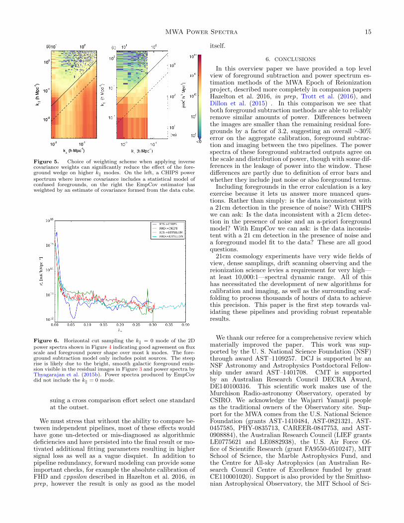
Before this last averaging step one can optionally in-clude an additional weighting by the known power spec-trum of a confused foreground in a process described inmore detail for these data by Trott et al. (2016). A 2Dforeground weighted power spectrum is shown in Figure5. The power spectra shown in Figure 7 show an excess ofpower in excess of the expected noise. This excess is no-tably similar between both calibration/foreground sub-traction pipelines. The amount of power in the excess,as compared with the error bars, also depends ratherdramatically on the range of k bins included in the finalaveraging to the 1D. These are discussed in more detailin section 4.1.

3.6. Power Spectrum #3: Empirical Covariance

The EmpCov power-spectrum estimation method com-putes both 2D and 1D power spectra using the quadraticestimator formalism. The method and its applicationto this data is described in more detail by Dillon et al.(2015) .

The quadratic estimator method of Liu & Tegmark(2011) treats foreground residuals in maps as a form ofcorrelated noise and simultaneously downweights bothnoisy and foreground-dominated modes, keeping trackof the extra variance they introduce into power spec-trum estimates. This technique can be computationallydemanding but using acceleration techniques describedby Dillon et al. (2013), has been applied to the previousMWA 32T results of Dillon et al. (2014) while a very sim-ilar technique, working on visibilities rather than mapsbut also using the data itself to estimate covariance, wasused for the recent PAPER 64 results of Ali et al. (2015).Dillon et al. (2015) build on these methods to mitigateerrors introduced by imperfect mapmaking and instru-ment modeling through empirical covariance estimation,assuming all data covariance is sourced by foregrounds.

EmpCov takes as input FHD calibrated images withforegrounds subtracted as well as possible, split intoeven and odd time-slices and averaged over many ob-servations. The differences between the even and oddtime-slices, which are assumed to be pure noise, are usedto calibrate the system temperature in a noise modelderived from observation time in uv cells. In orderto avoid directly propagating instrumental chromaticityinto the foreground residual covariance models (Dillonet al. 2015), EmpCov uses the data itself to properlydownweight residual foregrounds as seen by the instru-ment. It does this by estimating the frequency-frequencyforeground residual covariance in annuli in uvf space, as-suming that different uv cells independently sample theforeground residuals. This assumption, similar to thatmade by CHIPS, allows the combined foreground andnoise covariance to be inverted directly and used to down-weight the cubes when binning into 2D (and eventually

MWA Power Spectra 11

1D) band powers. As part of the quadratic estimatorformalism, EmpCovalso calculates error covariances andwindow functions (i.e. horizontal error bars). The result-ing power spectrum is shown in Figures 5 and 7.

3.7. Benefits of Comparison

One benefit from having multiple pipelines is the free-dom to investigate different optimization axes. The de-sign of the εppsilon power spectrum estimator empha-sizes speed and relative simplicity, choices motivated bythe need to understand the effect, on the power spectrum,of processing decisions such as observation protocol, flag-ging, and calibration. Using εppsilon we have discoveredand corrected multiple systematic effects, primarily thoseof a spectral nature which were not obvious in imagingbut quite apparent in the 2D power spectrum. With theability to quickly form power spectra on different sets ofdata, εppsilon has been an important tool for selectingsets of high quality data.

In contrast, CHIPS starts from time-ordered data andin its calculations emphasizes a more full accounting ofinstrumental and residual foreground covariance. Notonly does this higher resolution covariance calculationprovide a more accurate accounting of the instrumentalwindow function on the power spectrum, but it also al-lows for more precise weighting schemes based on knowl-edge of the statistical properties of the residual fore-grounds. This is useful when making 1D power spectrawhere foreground-like modes can be downweighted in theaverage.

Somewhere in the middle of these two is Emp-Cov which, like εppsilon uses image cubes and associ-ated weighting variances but performs a more formalquadratic estimator in which additional covariances canbe downweighted and the effects of the instrument win-dow function be factored into the calculation of the powerspectrum bins and error bars. It also demonstrates theimpact of inverse covariance weighting by forming a mea-sure of covariance from the data. This measure encapsu-lates both the residual foregrounds modeled by CHIPS aswell as any other residuals resulting from mis-calibration.

4. COMPARISON DISCUSSION

Inspecting a comparison of the images and power spec-tra reveals several common features. Images beforeand after foreground subtraction are shown in Figure 3,presented in the natural weighting used by the powerspectrum estimators without application of any furthercleaning. Putting the same 3 hours of MWA data intoeach pipeline, we inspect output images before and afterforeground subtraction. The pre foreground-subtracted(sometimes called the “dirty” image) have residuals atabout the 15% level; after foreground subtraction thedifferences are somewhat larger at 30%. Residuals inthe dirty maps are largest around bright sources. Thisis most likely due to slight differences in the calculationof image plane weights which are dramatically empha-sized by the broad psf from the natural weighting. Asevidenced by the clean residual maps, the point sourcesubtraction is well modeled when subtracted in the vis-ibilities. The foreground subtracted images (sometimescalled “residual” images) show a much closer agreementboth around the subtracted sources and in the large scale

structure. Large scale structure is more difficult to dis-tinguish. Inspection of the snapshot images before av-eraging in time and frequency revealed that the struc-ture is consistent across both time and frequency, whichsuggests real Galactic emission rather than sidelobes oraliasing.

4.1. Power Spectra

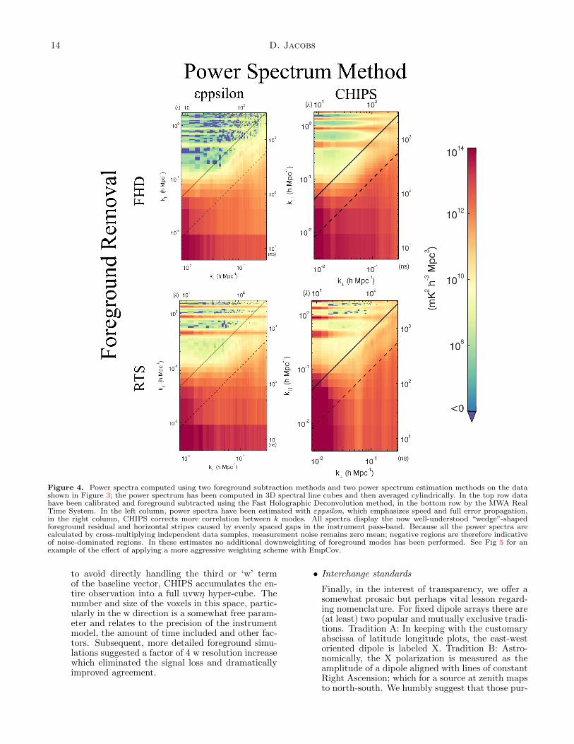
We apply both εppsilon and the unweighted version ofCHIPS to both of our calibration and foreground sub-traction pipes to produce a total of four different powerspectra (Figures 4 and 6). Each power spectrum estima-tor has been developed to target the output from a “pri-mary” calibration and foreground subtraction process—the diagonal panels of Figure 4—and have been highlyoptimized to that up-stream source of data. The off-diagonal power spectra were created using auxiliary linkswhich import the data and the metadata produced by theforeground subtraction step. Since they are less highlyoptimized, lacking as they do the advantage of a closeworking relationship, these pathways represent an upperlimit on the variance to be expected from small analysisdifferences but allow us to look for effects common toforeground subtraction or to power spectrum method.

Properties shared by all are the large amount ofpower at low k‖ roughly at an amplitude of 1015

mK2/(Mpc/h)3. This emission is approximately flatover most of k⊥ but rises steeply rise at low k⊥. Theamplitude agreement is particularly apparent in Figure6 where we plot a slice of the 2D power spectrum atk‖ = 0 where most foreground power is expected to lie.A model of smooth galactic emission has not been sub-tracted which likely contributes to this steep rise. The“wedge” shaped linear dependance on baseline length inthe 2D power spectra is due to the inherently chromaticresponse of a wide field instrument to smooth spectrumforegrounds; sources entering far from the phase centerappear as bright pixels at higher k‖ with sources on thehorizon at the edge indicated by Figure 4’s solid blackline. The solid and dotted lines in the figure indicate theupper boundaries of power from sources at the horizonand at the beam half power point, respectively. Withthe exception of some instrumental features foregroundpower is well isolated within this expected boundary.This emission is also visible in the image cubes as side-lobes extending from outside of the imaged area whichmove as function of frequency. Observations recordedwhen the Galactic plane is near the horizon have a muchlarger wedge component and have been excluded fromthis analysis. See Thyagarajan et al. (2015a), Thyagara-jan et al. (2015b) and Pober et al. (2016) for a detaileddiscussion of the foreground contributions to the powerspectra in this data.

The two main instrumental systematics are horizontalstriping due to missing or poorly calibrated data at theedges of regular coarse passbands and vertical stripingdue to spectral variation near uneven uvf sampling. Asdescribed in section 2, the MWA reads out spectra whichare divided into 1.28 MHz wide “coarse bands”. Thesebands have small known aliasing and gain instabilities inthe edge channels and so during initial flagging we flagthe edge-most 85kHz. This regular gap in the spectracorresponds to a poor sampling in Fourier space at in-

12 D. Jacobs

teger values of η = 781ns or k‖ = 0.45hMpc−1. In the2D power spectrum this manifests as horizontal stripesof high power which are in fact sidelobes of the fore-ground wedge, and higher error bars reflecting lack ofinformation about these modes. These sidelobes can beminimized by working to improve the accuracy of thepassband calibration and so have fewer flagged channels.They can also be downweighted by accounting for thecovariance between modes as is done by EmpCov.

A similar issue also arises from gaps in the uv coverage.In places where coverage is not uniform –such as at longerbaseline lengths where baseline density drops as 1/r2–beam weights can vary dramatically as a function of fre-quency leading to a vertical striping effect. It is mostprominent above |u| > 100λ or k⊥ > 0.1hMpc−1 whichcorresponds to when uv sampling begins to drop belowunity beyond the densest part of the MWA core. Thiseffect can be ameliorated by using an accurate modelfor the beam and array positions to grid these samplesaccording to the optimal mapmaking procedure, the ap-proach taken by the FHD imager, or the CHIPS approachof calculating and inverting the full instrumental covari-ance.

The most noticeable difference between the differentpipeline paths is in the power level in the window abovethe horizon and below the first coarse passband line (be-tween 0.1 and 0.3 k‖ and 0.01 and 0.05 k⊥). FHD toεppsilon displays a noise-like window in the 2D space,with a number of points dipping below zero while theother methods are noise like only at at much higher ks.One commonality between all power spectra with thispositive bias is a relatively higher amplitude of the coarsepassband lines.

The relative amplitude of the vertical striping is prob-ably the largest difference between the four power spec-trum methods. FHD-εppsilon sees vertical stripinglargely consistent with noise, the other methods seethe striping at varying levels with both CHIPS spectrashowing the largest. As discussed in detail by Moraleset al. (2012) and shown in data by Pober et al. (2016),this vertical striping is very sensitive to the accuracy ofthe weights used to average multiple samples together.εppsilon relies on the imager (FHD or RTS) to simulatethe instrument and generate optimally weighted mapswhile CHIPS uses an internal instrument model to calcu-late covariance. FHD used the second generation Sutinjoet al. (2015) beam model which takes into account cross-coupling within a tile while the rest used an analyticshort-dipole approximation.

We also compare the results of CHIPS and EmpCovusing analogous foreground downweighting schemes. Aquantitative comparison of these power spectra is dif-ficult, since the quadratic estimator’s downweightingscheme does not preserve foreground power. However,the results in Figure 5 are largely similar, showing the fa-miliar wedge structure and the brightest foreground con-tamination at low k⊥ where galactic foregrounds dom-inate. EmpCov excludes long baselines where coverageand sensitivity is poor and as such does not probe to thesame range in k⊥ as CHIPS. EmpCov appears to moresuccessfully remove foreground contamination near thewedge, which likely means that the foreground modelsemployed in CHIPS have room for improvement. Like-wise, EmpCov can successfully remove the lines in con-

stant k‖ that arise from flagged channels due to theMWA’s coarse band structure, but is still contaminatedby the 90 m cable reflection at k‖ ≈ 0.45 hMpc−1 (Dillonet al. (2015) ).

The final analysis step is to average into 1D powerspectra along shells of constant k. These are shown inFigure 7 for three of the four analysis tracks1 shown inFigure 4 with the addition of the Dillon et al. (2015)points and a theoretical sensitivity curve calculated usingthe 21CMSENSE sensitivity code2 by Pober et al. (2014).

The positive biases visible in the 2D power spectra arealso apparent here. Only a few points are fully consis-tent with zero at 2σ; however, most are very close tothe theoretical sensitivity curve and have errors match-ing those predicted for noise. The power spectra fallinto two groups, those calculated from input image cubes(εppsilon and EmpCov) and those calculated directlyfrom visibilities using CHIPS. The image-based pointsare somewhat deeper at low k, as noted in the 2D plots.Points from CHIPS are biased more strongly at low k butthe slope is flatter and converges with the other pipelinesat higher k.

4.2. CHIPS bias and the interpretation of error bars

Part of the CHIPS bias is due to the calculationof weightings. Default CHIPS analysis uses a statis-tical model of confused foregrounds to downweight bi-ased modes, particularly those correlated with the wedgepower. For this reason it is desirable to include thewedge modes in that 1D average. However it significantlychanges the interpretation of error bars; points in whicha significant amount of power have been downweightedwill have error bars much larger than thermal. In theinterest of comparing with the other methods, the powerspectra in Figures 4, 6 and 7 have been calculated usingpoints only lying outside the wedge horizon. This limitsthe amount of wedge-to-window covariance CHIPS canremove and contributes to the larger bias.

Including the full wedge in the CHIPS covariance cal-culation offers foreground suppression, but also intro-duces a foreground component into the error bars. Com-pare in Figure 8 the RTS→CHIPS power spectrum inFigure 7 with that given by Trott et al. (2016) whichused the same data shown here, though only 1/3 of the30MHz band. In both, CHIPS has downweighted by amodel of foreground covariance formed by propagatinga statistical model of confused sources. The only differ-ence is that black excludes the wedge but red does not.When the wedge is included the modeled foregrounds inthose voxels dominate the covariance weights. Applyingthese weights essentially moves the foreground bias intothe error bars and asserts that, given our best model offoregrounds, the power spectra are completely consistentwith noise and foregrounds.

The power spectra in Figure 7 show the range of re-sults possible given the same input data. Though they donot all agree, they do paint a consistent picture. Differ-ences partly come from the definition of error bars but

1The RTS→εppsilon spectrum is excluded here because at thetime of this analysis the RTS did not produce absolutely normalizedimage-plane uncertainties which are necessary to calculate 1D errorbars.

2github.com/jpober/21cmsense/

MWA Power Spectra 13

also indicate the relative difficulty of methods. Meth-ods which rely on an imager seem to perform somewhatbetter. This is perhaps unsurprising. CHIPS computesthe instrumental correlation matrix in visibility space us-ing beam, bandpass, etc. As the CHIPS analysis existsentirely in the visibility space, errors in modeling the in-strument are perhaps more difficult to detect than theyare in the image space. However, we do not suggest thatvisibility-based calculations like CHIPS are doomed tofailure; rather the opposite. The instrument models willcontinue to improve, and this improvement will be easilyvalidated by comparison with the other pipelines.

5. LESSONS FROM COMPARING INDEPENDENTPIPELINES

A data analysis pipeline is necessarily built on a com-plex software framework which is only approximately de-scribed in prose; it is therefore both difficult to perfectlyreplicate and susceptible to human error. Comparisonbetween independently developed analysis paths, eachwith their own strengths and limitations, is essential toplacing believable constraints on the Epoch of Reion-ization. The ongoing comparison between independentMWA pipelines has revealed a number of issues both sys-tematic (related to our understanding of the instrumentor foregrounds) and algorithmic (optimizing our use ofthis knowledge) which we will briefly mention here.

• Systematic example: cable reflections

As discussed above, one significant difference be-tween the two pipelines is the number of free pa-rameters fit in the calibration step, particularly inthe spectral dimension. Both calibration pipelinesbegin by calibrating each channel and then averag-ing over a number of axes. The RTS fits a low orderpolynomial, piecewise, to each of the 24 1.28MHzsub-band solutions, while FHD fits a similar orderpolynomial to the entire band’s calibration solu-tion. Inspection of power spectra calibrated us-ing the FHD scheme revealed previously unknownspectral features corresponding to reflections on theanalog cables at the -20dB level ( 1.5%). FHD cal-ibration now includes a fit for these reflections andthe feature is substantially reduced. These featuresare fully covered by the RTS fit (which uses of order10 times as many free parameters as FHD).

• Calibration example: number of sources

In early comparisons between RTS and FHD im-ages one immediately apparent difference was thesomewhat lower dynamic range of the RTS images.This was traced to the largest (at the time) dif-ference between the two approaches; RTS used themore traditional radio astronomy practice of cal-ibrating to a pointing on a bright source at thebeginning of each night and then transferring thecalibration to the rest of the observations, whereasFHD was calibrating against the foreground modelusing the cataloged sources within the field of view(a few thousand). This dramatically highlightedthe breakdown of approaches designed for tradi-tional dish telescopes with a narrow field of view.The MWA field of view is so wide, that even the cal-ibration pointing included many sources of bright-

ness comparable to the calibrator. These sourceswere not included in the calibration model and thuslimited the accuracy of the calibration. Also, ow-ing to the phased array beam steering, the primarybeam for the calibrator pointing is very differentfrom the beams used for the primary reionizationobservations, particularly in polarization response.So, though the instrument itself is highly stable intime over many hours, calibrations must be care-fully matched up with the observing parametersor experience a dramatic loss of imaging dynamicrange, both spatially and spectrally. The additionof “in field” calibration, where the foreground sub-traction model is also the calibration model, signif-icantly improved the RTS images and brought thetwo imagers into substantial agreement.

• Algorithmic example: full forward modeling for ab-solute calibration and signal loss

During the comparison process, one way in whichall pipeline results differed from each other is inthe overall amplitude of the power spectrum scale.Flux calibration, weightings, Fourier conventionsand signal loss must all be well understood for goodagreement to be reached. Signal loss, in particular,must be examined closely. Unintentional or un-avoidable down-weighting or subtraction of reion-ization signal could occur at multiple stages suchas bandpass calibration, uvf gridding, or inversecovariance weighting. These effects are best cali-brated via forward modeling of simulated sky in-puts. For example, detailed simulations of reion-ization signals through FHD and εppsilon foundthat in areas of dense uv sampling, simulated powerspectra experienced a 50% reduction of detectedpower (Hazelton et al. 2016, in prep). The act ofgridding complex visibilities into the uv-plane witha convolving kernel does not conserve the overallnormalization of the power spectrum. This effecthas been confirmed with simulations and results ina factor of 2 correction in the power spectrum; seeHazelton et al. 2016, in prep in prep. for a moredetailed explanation.

These simulated reionization data sets have beencalibrated internally by comparing outputs at everystep of the imaging and power spectrum process,and so are well understood at a detailed level, andsuitable for use as calibration standards for newpipelines.

• Algorithmic example: w-planes in power spectrumcalculation

Many of the differences found between power spec-tra during the comparison were traced to the post-foreground-subtraction steps, particularly the im-plementation of new imaging and power spectrumestimation codes. One example was an anomalousloss of power in CHIPS power spectra which par-ticularly affected longer baselines. CHIPS grids in

a coordinate space defined by the baseline vector ~band spectral mode η and then uses an instrumentmodel to diagonalize and sum in this sparse powerspectrum space. Unlike FHD which uses snapshots

14 D. Jacobs

Figure 4. Power spectra computed using two foreground subtraction methods and two power spectrum estimation methods on the datashown in Figure 3; the power spectrum has been computed in 3D spectral line cubes and then averaged cylindrically. In the top row datahave been calibrated and foreground subtracted using the Fast Holographic Deconvolution method, in the bottom row by the MWA RealTime System. In the left column, power spectra have been estimated with εppsilon, which emphasizes speed and full error propagation,in the right column, CHIPS corrects more correlation between k modes. All spectra display the now well-understood “wedge”-shapedforeground residual and horizontal stripes caused by evenly spaced gaps in the instrument pass-band. Because all the power spectra arecalculated by cross-multiplying independent data samples, measurement noise remains zero mean; negative regions are therefore indicativeof noise-dominated regions. In these estimates no additional downweighting of foreground modes has been performed. See Fig 5 for anexample of the effect of applying a more aggressive weighting scheme with EmpCov.

to avoid directly handling the third or ‘w’ termof the baseline vector, CHIPS accumulates the en-tire observation into a full uvwη hyper-cube. Thenumber and size of the voxels in this space, partic-ularly in the w direction is a somewhat free param-eter and relates to the precision of the instrumentmodel, the amount of time included and other fac-tors. Subsequent, more detailed foreground simu-lations suggested a factor of 4 w resolution increasewhich eliminated the signal loss and dramaticallyimproved agreement.

• Interchange standards

Finally, in the interest of transparency, we offer asomewhat prosaic but perhaps vital lesson regard-ing nomenclature. For fixed dipole arrays there are(at least) two popular and mutually exclusive tradi-tions. Tradition A: In keeping with the customaryabscissa of latitude longitude plots, the east-westoriented dipole is labeled X. Tradition B: Astro-nomically, the X polarization is measured as theamplitude of a dipole aligned with lines of constantRight Ascension; which for a source at zenith mapsto north-south. We humbly suggest that those pur-

MWA Power Spectra 15

Figure 5. Choice of weighting scheme when applying inversecovariance weights can significantly reduce the effect of the fore-ground wedge on higher k‖ modes. On the left, a CHIPS powerspectrum where inverse covariance includes a statistical model ofconfused foregrounds, on the right the EmpCov estimator hasweighted by an estimate of covariance formed from the data cube.

Figure 6. Horizontal cut sampling the k‖ = 0 mode of the 2Dpower spectra shown in Figure 4 indicating good agreement on fluxscale and foreground power shape over most k modes. The fore-ground subtraction model only includes point sources. The steeprise is likely due to the bright, smooth galactic foreground emis-sion visible in the residual images in Figure 3 and power spectra byThyagarajan et al. (2015b). Power spectra produced by EmpCovdid not include the k‖ = 0 mode.

suing a cross comparison effort select one standardat the outset.

We must stress that without the ability to compare be-tween independent pipelines, most of these effects wouldhave gone un-detected or mis-diagnosed as algorithmicdeficiencies and have persisted into the final result or mo-tivated additional fitting parameters resulting in highersignal loss as well as a vague disquiet. In addition topipeline redundancy, forward modeling can provide someimportant checks, for example the absolute calibration ofFHD and εppsilon described in Hazelton et al. 2016, inprep, however the result is only as good as the model

itself.

6. CONCLUSIONS

In this overview paper we have provided a top levelview of foreground subtraction and power spectrum es-timation methods of the MWA Epoch of Reionizationproject, described more completely in companion papersHazelton et al. 2016, in prep, Trott et al. (2016), andDillon et al. (2015) . In this comparison we see thatboth foreground subtraction methods are able to reliablyremove similar amounts of power. Differences betweenthe images are smaller than the remaining residual fore-grounds by a factor of 3.2, suggesting an overall ∼30%error on the aggregate calibration, foreground subtrac-tion and imaging between the two pipelines. The powerspectra of these foreground subtracted outputs agree onthe scale and distribution of power, though with some dif-ferences in the leakage of power into the window. Thesedifferences are partly due to definition of error bars andwhether they include just noise or also foreground terms.

Including foregrounds in the error calculation is a keyexercise because it lets us answer more nuanced ques-tions. Rather than simply: is the data inconsistent witha 21cm detection in the presence of noise? With CHIPSwe can ask: Is the data inconsistent with a 21cm detec-tion in the presence of noise and an a-priori foregroundmodel? With EmpCov we can ask: is the data inconsis-tent with a 21 cm detection in the presence of noise anda foreground model fit to the data? These are all goodquestions.

21cm cosmology experiments have very wide fields ofview, dense samplings, drift scanning observing and thereionization science levies a requirement for very high—at least 10,000:1—spectral dynamic range. All of thishas necessitated the development of new algorithms forcalibration and imaging, as well as the surrounding scaf-folding to process thousands of hours of data to achievethis precision. This paper is the first step towards val-idating these pipelines and providing robust repeatableresults.

We thank our referee for a comprehensive review whichmaterially improved the paper. This work was sup-ported by the U. S. National Science Foundation (NSF)through award AST–1109257. DCJ is supported by anNSF Astronomy and Astrophysics Postdoctoral Fellow-ship under award AST–1401708. CMT is supportedby an Australian Research Council DECRA Award,DE140100316. This scientific work makes use of theMurchison Radio-astronomy Observatory, operated byCSIRO. We acknowledge the Wajarri Yamatji peopleas the traditional owners of the Observatory site. Sup-port for the MWA comes from the U.S. National ScienceFoundation (grants AST-1410484, AST-0821321, AST-0457585, PHY-0835713, CAREER-0847753, and AST-0908884), the Australian Research Council (LIEF grantsLE0775621 and LE0882938), the U.S. Air Force Of-fice of Scientific Research (grant FA9550-0510247), MITSchool of Science, the Marble Astrophysics Fund, andthe Centre for All-sky Astrophysics (an Australian Re-search Council Centre of Excellence funded by grantCE110001020). Support is also provided by the Smithso-nian Astrophysical Observatory, the MIT School of Sci-

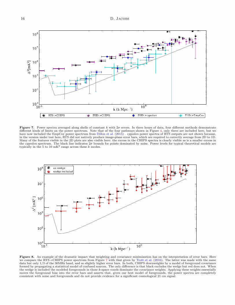
16 D. Jacobs

Figure 7. Power spectra averaged along shells of constant k with 2σ errors. In three hours of data, four different methods demonstratedifferent kinds of limits on the power spectrum. Note that of the four pathways shown in Figure 4, only three are included here, but wehave now included the EmpCov power spectrum from Dillon et al. (2015) . εppsilon power spectra of RTS outputs are not shown because,in the version under test here, RTS did not natively produce image-plane error bars, which are required to correctly average from 2D to 1D.Many of the features visible in the 2D plots are also visible here: the excess in the CHIPS spectra is clearly visible as is a smaller excess inthe εppsilon spectrum. The black line indicates 2σ bounds for points dominated by noise. Power levels for typical theoretical models aretypically in the 5 to 10 mK2 range across these k modes.

Figure 8. An example of the dramatic impact that weighting and covariance minimization has on the interpretation of error bars. Herewe compare the RTS→CHIPS power spectrum from Figure 7 with that given by Trott et al. (2016). The latter was made with the samedata but only 1/3 of the 30MHz band, and so slightly higher error bars. In both, CHIPS downweights by a model of foreground covarianceformed by propagating a statistical model of confused sources. The only difference is that black excludes the wedge but red does not. Whenthe wedge is included the modeled foregrounds in those k-space voxels dominate the covariance weights. Applying these weights essentiallymoves the foreground bias into the error bars and asserts that, given our best model of foregrounds, the power spectra are completelyconsistent with noise and foregrounds and do not provide evidence for a significant cosmological 21 cm signal.

MWA Power Spectra 17

ence, the Raman Research Institute, the Australian Na-tional University, and the Victoria University of Welling-ton (via grant MED-E1799 from the New Zealand Min-istry of Economic Development and an IBM Shared Uni-versity Research Grant). The Australian Federal gov-ernment provides additional support via the Common-wealth Scientific and Industrial Research Organisation(CSIRO), National Collaborative Research Infrastruc-ture Strategy, Education Investment Fund, and the Aus-tralia India Strategic Research Fund, and AstronomyAustralia Limited, under contract to Curtin University.We acknowledge the iVEC Petabyte Data Store, the Ini-tiative in Innovative Computing and the CUDA Centerfor Excellence sponsored by NVIDIA at Harvard Univer-sity, and the International Centre for Radio AstronomyResearch (ICRAR), a Joint Venture of Curtin Universityand The University of Western Australia, funded by theWestern Australian State government.

REFERENCES

Ali, Z. S. et al. 2015, ApJ, 809, 61 1, 3.6Barry, N., Hazelton, B., Sullivan, I., Morales, M. F., & Pober,

J. C. 2016, ArXiv e-prints 3.3Beardsley, A. et al. 2013, Monthly Notices of the Royal

Astronomical Society, 429, L5 1, 2.2, 3Bernardi, G., Mitchell, D. A., Ord, S. M., Greenhill, L. J.,

Pindor, B., Wayth, R. B., & Wyithe, J. S. B. 2011, MonthlyNotices of the Royal Astronomical Society, 413, 411 3.2

Bhatnagar, S., Rau, U., & Golap, K. 2013, ApJ, 770, 91 1, 3.2Bowman, J. et al. 2013, Publications of the Astronomical Society

of Australia, 30, 31 1Bowman, J., Morales, M., & Hewitt, J. 2009, The Astrophysical

Journal, 695, 183 1Chapman, E. et al. 2012, Monthly Notices of the Royal

Astronomical Society, 423, 2518 1—. 2013, Monthly Notices of the Royal Astronomical Society,

429, 165 1Chapman, E. et al. 2012, MNRAS, 423, 2518 1Condon, J. J., Cotton, W. D., Greisen, E. W., Yin, Q. F., Perley,

R. A., Taylor, G. B., & Broderick, J. J. 1998, TheAstronomical Journal, 115, 1693 a, 3

Cornwell, T. J., Voronkov, M. A., & Humphreys, B. 2012, inProc. SPIE, Vol. 8500, Image Reconstruction from IncompleteData VII, 85000L 3.2

Datta, A., Bowman, J. D., & Carilli, C. L. 2010, TheAstrophysical Journal, 724, 526 1

de Oliveira-Costa, A., Tegmark, M., Gaensler, B. M., Jonas, J.,Landecker, T. L., & Reich, P. 2008, Monthly Notices of theRoyal Astronomical Society, 388, 247, (c) Journal compilationc© 2008 RAS 1, a

Dillon, J., Liu, A., & Tegmark, M. 2013, Physical Review D, 87,43005 1, 3.6

Dillon, J. et al. 2014, Physical Review D, 89, 23002 1, 3.6Dillon, J. S. et al. 2015, Phys. Rev. D, 91, 123011 3, 2, 3.6, 4.1,

6, 7Dillon, J. S. et al. 2015, Phys. Rev. D, 91, 023002 1, 3.6Furlanetto, S. R., Oh, S. P., & Briggs, F. H. 2006, Physics

Reports, 433, 181, elsevier B.V. 1Gorski, K., Hivon, E., Banday, A., Wandelt, B., Hansen, F.,

Reinecke, M., & Bartelmann, M. 2005, The AstrophysicalJournal, 622, 759 3.1

Harker, G. et al. 2009, MNRAS, 397, 1138 1Heald, G. H. et al. 2015, A&A, 582, A123 1Hinshaw, G. et al. 2013, ApJS, 208, 19 1Hurley-Walker, N. et al. 2014, PASA, 31, 45 1, 3Intema, H. T., Jagannathan, P., Mooley, K. P., & Frail, D. A.

2016, ArXiv e-prints 1Jacobs, D. C. et al. 2011, The Astrophysical Journal, 734, L34 1Jacobs, D. C. et al. 2013, ApJ, 776, 108 1—. 2015, ApJ, 801, 51 1Jelic, V. et al. 2008, Monthly Notices of the Royal Astronomical

Society, 389, 1319, (c) Journal compilation c© 2008 RAS 1

Koopmans, L. et al. 2014, in Proceedings of AdvancingAstrophysics with the Square Kilometre Array (AASKA14). 9-13 June, 2014. Giardini Naxos, Italy.(http://pos.sissa.it/cgi-bin/reader/conf.cgi?confid=215), 1 1

Lane, W. M., Cotton, W. D., van Velzen, S., Clarke, T. E.,Kassim, N. E., Helmboldt, J. F., Lazio, T. J. W., & Cohen,A. S. 2014, MNRAS, 440, 327 3

Large, M., Cram, L., & Burgess, A. 1991, The Observatory, 111,72 3

Liu, A., Parsons, A. R., & Trott, C. M. 2014a, Phys. Rev. D, 90,023018 1

—. 2014b, Phys. Rev. D, 90, 023019 1Liu, A. & Tegmark, M. 2011, Physical Review D, 83, 103006 1,

3.5, 3.6Liu, A., Tegmark, M., & Zaldarriaga, M. 2009, MNRAS, 394,

1575, (c) Journal compilation c© 2009 RAS 1Lonsdale, C. J. et al. 2009, Proceedings of the IEEE, 97, 1497 2.1Mauch, T., Murphy, T., Buttery, H. J., Curran, J., Hunstead,

R. W., Piestrzynski, B., Robertson, J. G., & Sadler, E. M.2003, Monthly Notice of the Royal Astronomical Society, 342,1117 a, 3

Mitchell, D. A., Greenhill, L. J., Wayth, R. B., Sault, R. J.,Lonsdale, C. J., Cappallo, R. J., Morales, M. F., & Ord, S. M.2008, IEEE Journal of Selected Topics in Signal Processing, 2,707 3.1, 2, 3.2

Morales, M., Bowman, J., Cappallo, R., & Hewitt, J. 2006a, NewAstronomy Reviews 1

Morales, M., Bowman, J., & Hewitt, J. 2006b, The AstrophysicalJournal 1

Morales, M. F., Hazelton, B., Sullivan, I., & Beardsley, A. 2012,ApJ, 752, 137 1, 4.1

Morales, M. F. & Wyithe, J. S. B. 2010, Annual review ofastronomy and astrophysics, 48, 127, oise 1

Neben, A. R. et al. 2015, Radio Science, 50, 614 1Noordam, J. E. 2004, Ground-based Telescopes. Edited by

Oschmann, 5489, 817 3.1Offringa, A. R., de Bruyn, A. G., Zaroubi, S., & Biehl, M. 2010,

in RFI Mitigation Workshop, 36 2.4, 2Offringa, A. R. et al. 2014, MNRAS, 444, 606 1—. 2015, PASA, 32, 8 2.4Ord, S. M. et al. 2015, PASA, 32, 6 2.1Ord, S. M. et al. 2010, Publications of the Astronomical Society

of the Pacific, 122, 1353 1, 3.1, 2Parsons, A. R. et al. 2014, ApJ, 788, 106 1Parsons, A. R., Pober, J. C., Aguirre, J. E., Carilli, C. L., Jacobs,

D. C., & Moore, D. F. 2012, The Astrophysical Journal, 756,165 1, 3.4

Pindor, B., Wyithe, J. S. B., Mitchell, D. A., Ord, S. M., Wayth,R. B., & Greenhill, L. J. 2011, Publications of theAstronomical Society of Australia, 28, 46, (c) 2011Astronomical Society of Australia 3.2

Pober, J. C. et al. 2016, ApJ, 819, 8 1, 4.1Pober, J. C. et al. 2014, The Astrophysical Journal, 782, 66 1, 3,

4.1—. 2013, The Astrophysical Journal, 768, L36 1Pritchard, J. R. & Loeb, A. 2012, Reports on Progress in Physics,

75, 6901 1Salvini, S. & Wijnholds, S. J. 2014, A&A, 571, A97 3.2Santos, M. G. & Cooray, A. 2006, Physical Review D, 74, 83517 1Sullivan, I. S. et al. 2012, The Astrophysical Journal, 759, 17 1,

2, 3.2Sutinjo, A., O’Sullivan, J., Lenc, E., Wayth, R. B., Padhi, S.,

Hall, P., & Tingay, S. J. 2015, Radio Science, 50, 52 3.2, 4.1Tasse, C. et al. 2012, Comptes Rendus Physique, 13, 28, academie

des sciences 1Tegmark, M. 1997, ApJL, 480, L87 3.2Thompson, A. R., Moran, J. M., & Swenson, G. W. 2007,

Interferometry and Synthesis in Radio Astronomy, . (JohnWiley & Sons, 2007) 1

Thyagarajan, N. et al. 2015a, ApJ, 804, 14 1, 4.1—. 2015b, ApJL, 807, L28 1, 4.1, 6Thyagarajan, N. et al. 2013, The Astrophysical Journal, 776, 6

3.4Tingay, S. et al. 2013, Publications of the Astronomical Society of

Australia, 30, 7 1, 2.1Trott, C., Wayth, R., & Tingay, S. 2012, The Astrophysical

Journal, 757, 101 1

18 D. Jacobs

Trott, C. M. et al. 2016, ArXiv e-prints 2, 2, 3.5, 4.2, 6, 8Vedantham, H., Shankar, N. U., & Subrahmanyan, R. 2012a, The

Astrophysical Journal, 745, 176 1—. 2012b, The Astrophysical Journal, 745, 176 3.4Wayth, R. B. et al. 2015, PASA, 32, 25 1

Yatawatta, S. et al. 2013, Astronomy & Astrophysics, 550, 136 1Zaroubi, S. 2013, in Astrophysics and Space Science Library, Vol.

396, Astrophysics and Space Science Library, ed. T. Wiklind,B. Mobasher, & V. Bromm, 45 1