the negative credit risk premium puzzle: a limits to ... elect to use uk data to test our...
TRANSCRIPT
Discussion Paper Number: ICM-2015-07
Discussion Paper
The Negative Credit Risk Premium Puzzle: A Limits to Arbitrage Story
September 2015
Chris Godfrey ICMA Centre, Henley Business School, University of Reading
Chris Brooks ICMA Centre, Henley Business School, University of Reading

ii © Godfrey and Brooks, September 2015
The aim of this discussion paper series is to disseminate new research of academic distinction. Papers are preliminary drafts, circulated to stimulate discussion and critical comment. Henley Business School is triple accredited and home to over 100 academic faculty, who undertake research in a wide range of fields from ethics and finance to international business and marketing.
www.icmacentre.ac.uk
© Godfrey and Brooks, September 2015
Henley Discussion Paper Series
© Godfrey and Brooks, September 2015 1
The Negative Credit Risk Premium Puzzle: A Limits to Arbitrage Story
Abstract Prior research has documented that, counter-intuitively, high credit risk stocks earn lower – not
higher – returns than low credit risk stocks. In this paper we provide evidence against rational
expectations explanations, and show that a model incorporating limits-to-arbitrage factors is
capable of explaining this apparent anomaly. We demonstrate that the negative pricing of credit
stocks is driven by the underperformance of stocks which have both high credit risk and which
have suffered recent relative underperformance, and that their ongoing poor performance can
be explained by a mixture of four limits-to-arbitrage factors – idiosyncratic risk, turnover,
illiquidity and bid-ask spreads. Collectively, these impede the correction of mispricing by
arbitrageurs, especially on the short leg of the trade, where commonly reported returns are
unattainable.
Keywords behavioural finance, relative distress, credit risk premium puzzle, asset pricing, limits to arbitrage
JEL Classifications C31, C55, D03, G12
Acknowledgements We thank Bibek Bhatta, Darren Duxbury, Andreas Hoepner, Kim Kaivanto, Gulnur Muradoglu,
and participants at the Behavioural Finance Working Group Conference 2015, Queen Mary
University, for helpful comments. All errors are our own.
Contact Chris Godfrey, ICMA Centre, Henley Business School, University of Reading, Whiteknights,
Reading RG6 6BA, UK; tel: +44 (0)118 378 8239; email: [email protected]
ICMA Centre
2 © Godfrey and Brooks, September 2015
1 Introduction
1.1 Background and motivation
The usual assumption in the fixed income markets is that credit risk is positively priced – that is,
investors expect that exposure to credit risk will be compensated by higher returns. Yet a variety
of studies have found that it is actually rewarded by lower returns in cross-section among
equities: Dichev (1998), Chen et al. (2010) and Chou et al. (2010a) find credit risk to be
negatively priced for US equities when using accounting-based ratios such as the Altman’s
(1968) z-score and the Ohlson’s (1980) O-Score, as do Campbell et al. (2008) when employing a
hazard-rate score, and Avramov et al. (2009) when sorting stocks on the basis of their Standard
& Poor’s issuer rating.
Broadly, attempts to explain this paradox fall into one of two philosophical paradigms – a
rational pricing perspective and an investor behavioural one. Rational pricing arguments have
started with the presumption that shareholders are able to endogenously default on the value of
the firm’s debt, expecting to recover a portion of the firm’s value in bankruptcy resolution, and
that their default option becomes increasingly important close to the default boundary.
Approaches based on rational expectations, notably by George and Hwang (2010), Garlappi and
Yan (2011) and McQuade (2013), have received some prior empirical support but we present
evidence against these below. Since the UK features a bankruptcy regime which strongly favours
creditors and where shareholders are typically not able to strategically default on the firm’s debt,
we elect to use UK data to test our hypothesis; isolating the origin of the negative credit spread
anomaly is greatly simplified if endogenous default by shareholders can be ruled out as a cause
by the nature of the local bankruptcy code.
Focusing on behavioural arguments, we find that a simple combination of limits-to-arbitrage
factors is capable of subsuming the negative pricing of credit risk in cross-section: high credit risk
stocks have poor returns not because investors are switching attention to a bankruptcy recovery
process, where high distress firms choose low leverage or gain high exposure to innovations in
market volatility, but because high credit risk increases the dispersion of views on a firm’s
valuation, and allows them to become overpriced as excessively optimistic investors absorb the
available supply. Where such firms also have severe “limits-to-arbitrage” characteristics – for
instance, having high idiosyncratic volatility, high illiquidity, wide bid-ask spreads and low
turnover, these hinder the correction of such overpricing by arbitrageurs, so that they remain
persistently overpriced and suffer low returns. If they did not suffer from these limits-to-
arbitrage factors, arbitrageurs would be able to short them down to more rational values. We
Henley Discussion Paper Series
© Godfrey and Brooks, September 2015 3
thus provide a parsimonious explanation of the outstanding anomaly of the negative pricing of
credit risk among equities.
An important precursor to our work is the study by Ali et al (2003), discussed in detail below,
who provide an incomplete explanation for the book-to-market premium using limits-to-
arbitrage factors. The cross-sectional pricing of book-to-market is partially explained by the entry
of factors relating to investor sophistication and arbitrage costs – notably, idiosyncratic risk –
consistent with the Shleifer and Vishny (1997) thesis that risk associated with the volatility of
arbitrage returns deters arbitrage activity and is an important reason for the existence of
mispricing related to book-to-market. The book-to-market premium is significantly stronger
among portfolios with high values of limits-to-arbitrage factors than among stocks with low
costs of arbitrage, and there are significant interactions in cross-section between book-to-
market and a range of limits-to-arbitrage factors. The hint is that the book-to-market premium is
perpetuated by the high costs of arbitrage among some stocks.
The key intuition of this paper is that a similar model to that of Ali et al (2003), which explicitly
includes a rich variety of limits-to-arbitrage factors, ought to be capable of explaining another
outstanding anomaly, namely, that of the negative pricing of credit risk in equities. Through the
results presented in this paper, we argue that this is the case, and as such, it ought to be
understood as a consequence of frustrated arbitrage among some stocks, and that recourse to
rational expectations explanations is unnecessary.
2 The negative pricing of credit risk in equities
2.1 The negative credit spread anomaly in US data
The initial demonstrations of the negative credit spread anomaly define credit risk by means of
accounting ratios: using both Altman’s (1968) z-score and Ohlson’s (1980) O-Score, Dichev
(1998) finds default risk to be negatively priced for a sample of US stocks. With Ohlson’s (1980)
O-Score, Griffin and Lemmon (2002) find that distress risk is significantly negatively priced
among low book-to-market equity stocks. Ferguson and Shockley (2003) construct a market
value-weighted relative distress factor by double-sorting on Altman’s (1968) z-score and market
leverage in a similar way to the construction of the Fama-French (1993) factors, and find that it
yields a negative price for distress risk. Chou et al. (2010) employ a similarly-constructed market
value-weighted Altman’s (1968) z-score factor and find distress risk to be significantly negatively
priced in the cross-section for US stocks. Confirming, Chen et al. (2010) sort stocks into quintiles
of credit risk based on the Altman’s (1968) z-score and the Ohlson’s (1980) O-Score, and
ICMA Centre
4 © Godfrey and Brooks, September 2015
measure the resulting portfolios’ aggregate abnormal excess returns, finding that the quintile
with the highest credit risk by either measure earns less than the quintile with the lowest credit
risk, for both the Altman’s (1968) z-score, and the Ohlson’s (1980) O-Score.
The negative credit spread anomaly persists where credit risk is measured by means of hazard
rate measures: Campbell et al. (2008) find their hazard rate measure of default risk to be
negatively priced when excess returns against the Fama-French (1993) model are compared.
Chava and Purnanandam (2010) compare a hazard rate and an option-based expected default
frequency measure, and likewise find a negative pricing of credit default risk for the post-1980
period. The negative credit anomaly likewise persists when credit risk is measured using credit
rating agency ratings (Avramov et al., 2009).
If credit risk is implied using Credit Default Swap (hereafter CDS) spreads, Friewald et al (2014)
find a positive relationship between firms’ CDS-implied market prices of risk, and realised
returns, in apparent contradiction of the above findings. However, this study can be queried
regarding its sample, and from the theoretical point of view. Firstly, it uses CDS spreads for a
sample of only 675 US-based obligors, covering only a fraction of the sample of the stock
universe used by previous studies, and a sample which necessarily consists of the largest, most
liquid and least distressed firms. Secondly, it is heavily reliant upon the assumption that “the
market price of risk (the Sharpe ratio) must be the same for all contingent claims written on a
firm’s assets” (Friewald et al., 2014, p. 2419) to relate the implied risk of default from the CDS
market to the equity market. However, Kapadia and Pu (2012) find a lack of integration between
the equity and CDS markets, such that a sizeable number of stocks’ relationships are anomalous,
and that the integration in times-series between the two markets is related to firm-specific
impediments to arbitrage such as liquidity and idiosyncratic risk. In a similar vein, Choi and Kim
(2015) find that risk premia in the equity and bond markets are not integrated, and that the
discrepancies between the two vary with aggregate investor sentiment, concentrated on the
short-side of arbitrage portfolios and which is greatest when short-sale impediments are
present. The assumption that firms’ risk premia in the equity and CDS markets are necessarily
identical can therefore not be maintained empirically, but instead, the relationship between the
two is necessarily subject to behavioural and limits-to-arbitrage constraints.
2.2 The negative credit spread anomaly in UK and other international data
Agarwal and Taffler (2008) investigate the link between momentum and financial distress in the
UK using the Taffler (1983) z-score, and find evidence that credit risk is negatively priced. They
Henley Discussion Paper Series
© Godfrey and Brooks, September 2015 5
also observe significantly positive momentum effects only among stocks rated as high credit risk,
and conclude that asset price momentum is proxying for distress risk and is driven by financially
distressed firms. Their results again show that the negative pricing of distress risk is strongest
among the lowest Loser quintile and is not significant at the 5% level among any other
momentum quintile. The negative pricing of credit risk in the UK is confirmed by Agarwal and
Poshakwale (2010), who construct a z-score factor by a methodology similar to Chen et al.
(2010) above. A more recent paper by Agarwal and Bauer (2014) confirms that credit risk is
negatively priced in cross-section for the UK, whether measured by the Taffler (1983) z-score, a
Shumway (2001) hazard rate model, or a Merton (1974) distance-to-default measure.
These conclusions are confirmed by a number of more recent papers making broad international
surveys of the credit spread. Gao et al (2013) sort stocks from a wide range of countries on
Moody’s-KMV Expected Default Frequencies (hereafter, EDF), and find a significantly negative
cross-sectional pricing of credit risk for European stocks in aggregate, and for the UK in
particular. Eisdorfer et al (2013) construct Merton (1974) distance-to-default measures for the
stocks of a number of countries, and again find a significantly negative pricing of credit risk for
developed countries; for the UK, the pricing of credit risk is negative but insignificant.
2.3 Mispricing and rational expectations explanations for the negative credit spread anomaly
One class of explanations posits that the negative credit spread anomaly is an outcome of
investors maximising conventional utility functions under rational expectations; there are
therefore no behavioural, limits-to-arbitrage factors needed or mispricings to identify, but
rather, such explanations attempt to show how high credit risk stocks ought to be regarded,
paradoxically, as less risky than low credit risk stocks. However, we present here evidence against
four of the principal theories.
George and Hwang (2010) model the leverage choices of a hypothetical firm which suffers
distress costs if it enters into a state of financial distress, and argue that firms with high distress
costs will choose lower leverage levels, whilst having higher exposure to systematic risk. Firms
with low leverage will therefore tend to paradoxically experience lower returns, assuming
investors realise the returns predicted by the CAPM However, we show below that high credit
risk Loser stocks do not have significantly higher market betas than low credit risk Losers; since
we later show that the negative credit spread anomaly localises to such Loser stocks, it appears
that these firms do not experience significantly higher systemic risk.
ICMA Centre
6 © Godfrey and Brooks, September 2015
Another rational expectations theory which seeks to account for the negative pricing of credit
risk is provided by Garlappi and Yan (2011), who suggest that shareholders may seek to recover
part of the residual firm value by defaulting on their debt, after the resolution of debt default or
bankruptcy, and that high leverage actually reduces the equity beta when financial distress
looms, as shareholders switch attention from the volatile value of the distressed company to the
more stable value of the payoff they hope to achieve in the event of bankruptcy resolution. This
explanation is, however, reliant upon the creditor-friendly US bankruptcy code which gives
shareholders an expectation of meaningful recovery in the event of default; Garlappi and Yan
(2011) assert an average shareholder recovery of around 20% of asset value for US stocks.
In a similar vein, Eisdorfer et al (2012) construct a model of company default and investor utility
under which the firm’s option to default, considered to be endogenous, is valuable for a
distressed company. Investors fail to appreciate the value of this option, however, leading them
to strongly undervalue distressed stocks. However, the magnitude of this embedded “option to
default” appear unrealistically large in the simulated results to produce the observed negative
credit spread: the mean (median) relative misvaluation between the market and the model is a
very surprising 1527% (678%) for the most undervalued tertile – that is, the model predicts that
the true value of these firms, including the claimed value of the option to default, is over 15
times (over 6 times) the market value of the firm. For a full third of the market to be apparently
undervalued by such a large margin surely suggests that the Eisdorfer et al. (2012) model of
company valuation is unrealistic.
McQuade (2013) proposes a further model in which shareholders endogenously default on the
firm’s debt, and where excess expected returns are a combination of the risk premia due to its
exposure to productivity risk and to its exposure to innovations in market volatility. Although the
recovery rate is not directly specified but is a function of the costs of bankruptcy, the model
produces a recovery rate of approximately 51% for shareholders (McQuade, 2013, p. 32). Part of
the firm’s equity value therefore consists of the equity holders’ default option. Indeed, in
financial distress, most of the equity value consists of the default option, and the debt of a firm
which is extremely close to default actually benefits from an increase in market volatility and
thus hedges market volatility risk. Healthy firms therefore have higher variance risk premia than
distressed firms, and a portfolio which is long healthy firms and short distressed firms should
earn positive abnormal excess returns, and so giving rise to the observed negative credit spread.
Another theory, advanced by Avramov et al (2011), seeks to explain the low returns earned by
both high credit risk stocks and high idiosyncratic volatility stocks in a rational expectations
framework. They make use of the “relative share” concept of Menzly et al. (2004) as the ratio of
Henley Discussion Paper Series
© Godfrey and Brooks, September 2015 7
the long-run dividend share of a firm as a proportion of its current dividend share, with dividend
share being the fraction of the dividend paid by the firm relative to the aggregate dividend. They
propose that firms with high relative share have “high cashflow duration,” and are highly
exposed to shocks to the persistent economic growth rate, which causes rational investors to
demand higher risk premia, leading to higher expected returns. By contrast, firms with low
relative share have “low cashflow duration” and are more sensitive to firm-specific dividend
shocks but have reduced exposure to shocks to the persistent economic growth rate, and hence
low risk premia and low expected returns. One prediction of the model is that investors regard
long-run cash flows as more risky than short-term cash flows, and so apply high risk premia to
them, whereas risk premia on low duration cash flows are negligible.
Avramov et al. (2011) hypothesise that these low relative share firms are highly sensitive to firm-
specific dividend shocks, which leads them to have high idiosyncratic volatility. Since the large
majority of a firm’s return volatility is unsystematic, idiosyncratic shocks are assumed to be the
primary cause of defaults, as firm default is modelled in a Merton (1974) framework where
default occurs if the firm’s value drops below the face value of the firm’s debt. These low relative
share firms are therefore predicted to have low returns, high idiosyncratic volatility, high default
risk and elevated levels of earnings forecast dispersion. In this framework, default probability and
idiosyncratic volatility are closely related. This model therefore uses dividend share and
exposure to the long-term economic growth rate to explain why high default risk stocks should
have low returns.
In support of their hypothesis, Avramov et al. (2011) empirically observe a monotonic increase
in idiosyncratic risk in portfolios sorted into deciles on default probability, assessed using a
Campbell et al. (2008) hazard rate measure, and a monotonic increase in default probability in
portfolios sorted into deciles on idiosyncratic risk. However, some weaknesses do emerge in the
empirical testing of the model: some of the dividend share modelling appears unrealistic, with
the petroleum industry forecast to yield 38.5% of the total aggregate US corporate dividend in
the long term, up from 11.4% at the start of the sample period. The model also predicts an
apparent growth stock premium, if dividend-to-price is used as a proxy for book-to-market,
contrary to the usual empirical finding of a value premium. For the highest decile of distress risk,
relative share is abnormally high, contrary to predictions, and share ratio is not priced in cross-
sectional regressions when explaining the returns of portfolios sorted on distress risk. More
seriously, the model has to explain why investors are predominantly concerned only about
shocks to the long-term economic growth rate, and are apparently unconcerned about their
ICMA Centre
8 © Godfrey and Brooks, September 2015
exposure to distress risk. We provide further evidence against the Avramov et al (2011) model
below, in more fully testing the relationship between returns, idiosyncratic risk and credit risk.
A similar hypothesis is advanced by Radwanski (2010), which relies upon a model economy in
which a cointegrating relationship exists between aggregate consumption and dividends.
Distressed firms have short expected maturities of cash flows, so that their prices are not as
strongly influenced by shocks in the persistent conditional mean of consumption growth; they
are therefore hypothesised to be safer, and hence have lower expected returns. Non-distressed
firms are argued to be more exposed to these shocks, owing to the persistence of their effects in
the long term. In simulations, the model is able to qualitatively match some empirical features of
returns of portfolios sorted on credit risk, but is unable to generate the observed negative credit
spread premia. It also shares the drawback of the Avramov et al. (2011) model, in failing to
explain intuitively why investors should not care about their firms going bust in the short-term
under the influence of short-term shocks.
Another class of explanations posits that investors universally misprice some aspect of risk in
high credit risk stocks, and that it is this general failure to properly assess risk which generates
the negative credit spread anomaly. For instance, Ozdagli (2013) proposes a model of company
default and investor utility which suggests that if default probability is assessed under the risk-
neutral measure rather than the real measure, then returns are increasing rather than decreasing
with risk-neutral default likelihood. Risk neutral default probabilities of default are therefore
different from probabilities under the real measure, and they suggest that implied risk-neutral
default probabilities from Credit Default Swap (CDS) spreads might provide empirical proof.
However, as noted previously, Kapadia and Pu (2012) find a lack of integration between the
equity and CDS markets, so that risk premia are not integrated between them where limits-to-
arbitrage factors are strong. If limits-to-arbitrage factors and credit risk are correlated, as we
argue below, then inferences from CDS data on firms’ default risk will not transfer well to the
equity market in precisely those cases where default risk is high, and hence results obtained by
this method may be expected to be less reliable there.
2.4 Evidence against rational expectations explanations for the negative credit spread anomaly
The rational expectations hypotheses all encounter serious difficulties in explaining the negative
credit spread anomaly. In particular, they all assume that the task they must accomplish is to
explain why expected returns decrease with increasing credit risk, when the evidence is that this
is not the case; on the contrary, investors do, in fact, expect to be rewarded for bearing exposure
Henley Discussion Paper Series
© Godfrey and Brooks, September 2015 9
to credit risk. Chava and Purnanandam (2010) derive ex ante expected returns from implicit
costs of capital, and find that there is a significantly positive relationship between default risk
and expected returns in cross section. A similar paradox occurs with respect to idiosyncratic
volatility: investors ex ante expect to be rewarded for bearing exposure to elevated levels of
idiosyncratic volatility (Spiegel and Wang, 2005; Fu, 2009). The challenge, then, is not to explain
why expected returns for high credit risk stocks should be low, but why investors receive low ex
post returns when they anticipate high, and this points to an analysis of investor behaviour and
market function rather than of expected returns.
Secondly, the Garlappi and Yan (2011), Eisdorfer et al (2012) and McQuade (2013) hypotheses
rely upon shareholders being able to recover part of the firm’s value in bankruptcy. Indeed, the
McQuade (2013) hypothesis is critically reliant upon shareholders’ endogenous default, since it
fails to match the credit spread on junk bonds when the default boundary is specified
exogenously; it succeeds “if and only if equity holders are allowed to optimally decide when to
default.”(McQuade, 2013, p. 2) Secondly, the model also predicts that abnormal excess returns
from momentum strategies should be negative among low credit risk stocks.
By the same token, these hypotheses imply that the negative credit spread ought to disappear in
the UK context, where creditors’ rights are far stronger, since UK shareholders generally recover
negligible amounts from a bankruptcy process. In the international survey of La Porta et al.
(1998), the UK achieves the maximum Creditor Rights score of four, whereas the US scores the
minimum of one. Davydenko and Franks (2008) find that the median recovery rate for senior
secured debt in bankruptcy is 82% in the UK compared with 61% in Germany and 39% in France,
in a survey of companies which have defaulted on bank debt. Unsecured creditors, on the other
hand, fare badly in the UK in the event of bankruptcy; “recovery rates for junior creditors are
negligible” (Davydenko and Franks, 2008, p. 571), confirmed by Blazy et al. (2013). Though
Franks and Sanzhar (2006) show that UK banks are willing to engage in debt forgiveness when
listed distressed firms seek to raise equity as part of a recovery process, Franks and Sussman
(2005) find that while UK banks typically do make efforts to rescue a distressed firm, they tend
to be very tough in negotiating with it, so that UK firms do not default strategically in order to
extract concessions from banks. They also find that banks tend to time their liquidation
decisions as secured creditors close to “when the value of the firm equals the value of the bank’s
collateral, with little left over to junior creditors” (Franks and Sussman, 2005, p. 67). If little is left
over for junior unsecured creditors, it is surely safe to conclude that UK shareholders’ residual
claim can be assumed to be negligible once default has occurred.
ICMA Centre
10 © Godfrey and Brooks, September 2015
If the above hypotheses reliant upon endogenous default were true, these ought to indicate that
UK shareholders would tend to expect a negligible recovery in the event of default. If they
cannot switch attention to a stable payoff from bankruptcy resolution in the manner they posit
is possible in the US, the negative credit spread ought to disappear in the UK. That it does not
indicates that the Garlappi and Yan (2011), Eisdorfer et al (2012) and McQuade (2013)
explanations do not receive empirical support.
3 Limits to arbitrage factors in asset pricing
3.1 The mode of action of limits to arbitrage
The theory of limits to arbitrage, as described by Shleifer and Vishny (1997), holds that arbitrage
in financial markets is costly to execute, is risky, and tends to be undertaken by participants who
operate with limited capital and whose shareholders may withdraw capital from arbitrageurs’
operations if they experience a loss. Professional arbitrageurs therefore stand exposed to
fluctuations in asset prices which drive them further away from fundamental values, so that
arbitrage trades which would be ultimately profitable in the long-term may show losses in the
short-term, and the threat of capital withdrawal by shareholders in such circumstances makes
them more cautious in entering into arbitrage trades, and less effective in bringing about market
efficiency. They argue that since arbitrageurs are typically not well-diversified, high volatility
arising from noise trader sentiment makes arbitrage unattractive if it does not lead to increased
expected profits. In particular, idiosyncratic volatility discourages arbitrage since it cannot be
hedged. Financial market anomalies are therefore more likely to persist where market factors
make arbitrage more risky or costly to execute.
To this, Miller (1977) adds the insight that arbitrage is more likely to be constrained on the leg of
the trade requiring a short sale; selling a share short requires first that it be borrowed from a
willing counterparty, and the facility for stock lending in sufficient size may be limited;
additionally, a short seller does not receive the cash equivalent of the share upon the sale, as the
Black-Scholes (1973) model assumes, which instead is normally retained as collateral by the
stock lending agent. The short seller must also compensate the stock lending counterparty for all
dividends received during the borrowing period, in addition to paying a stock lending fee.
Although many proposed limits-to-arbitrage factors ought in theory to result in overpricing and
underpricing with equal regularity, the additional difficulty of shorting means that the net effect
ought to be that overpricing is more prevalent, owing to the additional difficulty of taking short
positions compared to long ones. We should therefore expect anomalies to derive their
Henley Discussion Paper Series
© Godfrey and Brooks, September 2015 11
apparent profits from the short leg of the arbitrage transaction which would have to be effected
in order to exploit them, as Finn et al (1999) find for the value and size premia. We should also
expected to find that stocks with high levels of limits-to-arbitrage factors will tend to suffer low
returns, owing to their persistent overpricing.
We may distinguish between three categories of limits-to-arbitrage factors:1
Firstly, factors which impede the adoption of short positions but not long positions, and so
hinder the correction of overpricing but not underpricing: these include short selling costs, as
modelled in Gromb and Vayanos (2010); whether collateral is classed as “general collateral” or
“special collateral,” as investigated by Ali and Trombley (2006); and low institutional ownership,
which may limit the number of shares available to borrow, as studied by Duan et al (2010) and
Ali and Trombley (2006).
Secondly, factors which impede the adoption of long positions but not short positions, and
hinder the correction of underpricing. The factors in this category may include concentration
limits by asset managers, but these are not likely to be significant.
Thirdly, limits-to-arbitrage factors which are symmetrical in impeding arbitrage positions in
either direction. These include high leverage costs as modelled in Gromb and Vayanos (2010);
wide bid-ask spreads; high illiquidity; low turnover; and high idiosyncratic volatility. In practice,
though these ought to have bi-directional action, we expect to find that the additional
constraints imposed by the difficulty of taking short positions will lead to these factors resulting
in more overpricing than underpricing, that is, stocks with more severe levels of these factors will
on average manifest lower returns. Since these factors have bidirectional effects, we should
expect to find that recent relative winners and losers, as ranked by prior returns, will manifest
more severe levels of these factors, specifically, low levels of turnover, high illiquidity, high bid-
ask spreads and high idiosyncratic volatility. Further, stocks which have recently experienced
severe levels of these factors ought to display stronger momentum effects.
Ordinarily, under classical asset pricing theory, we would expect that sources of risk which are
systematic should earn positive risk premia – that is, investors will receive higher returns for
accepting exposure to them. In the case of factors which represent limits to arbitrage, however,
there is evidence that the reverse applies, and these factors are frequently found to be negatively
priced in cross-section, that is, stocks with higher exposure to the limits-to-arbitrage factor
suffer lower, rather than higher, ex-post returns. While this may at first seem paradoxical, it arises
as a necessary consequence of the tendency of such limits-to-arbitrage factors to impede 1 We are grateful to Kim Kaivanto for suggesting this taxonomy.
ICMA Centre
12 © Godfrey and Brooks, September 2015
arbitrage by frustrating the shorting of the stock. All else being equal, stocks with higher
exposure to such factors therefore tend to remain overvalued, and suffer lower realised returns
as a result.
If a limits-to-arbitrage factor impedes both the taking of long and short positions, then we
should expect that it would contribute to both the elevated returns of prior Winners, as ranked
by prior returns, and the depressed returns of prior Losers. Absent these factors, good (bad)
news would be reflected immediately in the price of these stocks, but in their presence, the
inability of arbitrageurs to force up (down) the price to the new fundamental value by taking
sizeable long (short) positions is hindered, so that stock prices take longer to drift upwards
(downwards) to the new fundamental value, and so exhibiting multi-period price momentum.
We should therefore expect that momentum profits will tend to be stronger among stocks
where limits-to-arbitrage factors are stronger. Additionally, if limits-to-arbitrage factors tend to
induce abnormally low returns by frustrating the shorting of a stock, then we might expect that
this would exacerbate the poor returns of Losers in cross-sectional momentum strategies, so
that momentum profits will tend to derive predominantly from the underperformance of Losers
rather than the superior performance of Winners among stocks experiencing higher limits to
arbitrage.
In this paper, we consider four direct limits-to-arbitrage factors, namely, idiosyncratic volatility,
illiquidity, the bid-ask spread and turnover. Idiosyncratic volatility and illiquidity have been
established as forming limits-to-arbitrage factors in US data by Duan et al. (2010), and the bid-
ask spread is an obvious addition. Further, low turnover makes arbitrage more difficult by
increasing the time taken for an arbitrageur to enter or exit a position in size. It should be noted
that this apparent negative pricing of limits-to-arbitrage factors in cross-section is a different
phenomenon from the positive pricing of innovations in the aggregate level of these factors in
time series. For example, Pástor and Stambaugh (2003) argue that aggregate market-wide
illiquidity forms a non-diversifiable, systemic risk factor, and they posit that investors are
compensated for bearing exposure to unexpected innovations in its level. However, the pricing
of a stock’s time-series weighting on the unexpected innovations in aggregate market-wide
illiquidity may be very different from the pricing effects induced by the limits to arbitrage arising
from its own illiquidity.
3.2 Turnover as a limit to arbitrage
If a stock has low turnover, it is likely to be more difficult to enter and exit positions in a timely
manner, and hence the arbitrageur is likely to be more exposed to adverse stock movements in
Henley Discussion Paper Series
© Godfrey and Brooks, September 2015 13
an arbitrage transaction. We would expect momentum profits to be greater among stocks with
higher turnover, as arbitrageurs are hindered from correcting the underpricing of Winners and
the overpricing of Losers. We would also expect turnover to be overall positively priced in cross-
section, since for an increase in turnover, short selling to correct overvaluation would become
easier to effect, overvaluation would decrease, and ex-post returns would increase. There is
some evidence that turnover functions in this manner in the limits-to-arbitrage literature: Ali
and Trombley (2006) find prior month turnover to be positively priced in cross-section when
prior six-month returns, price, size, a proxy for the likelihood of high short selling costs and
analyst coverage are also included. As the limits-to-arbitrage hypothesis would predict, this is
predominantly driven by the underperformance of low turnover Losers compared to the
performance of high turnover Losers, where the difficulty and cost of shorting is likely to be most
difficult to achieve. Turnover causes a differential in return among Losers but not Winners, that
is, low turnover Losers underperform high turnover Losers, providing further evidence that low
turnover frustrates the short leg but not the long leg of arbitrage trades. Further evidence comes
from Avramov et al. (2009), where the same pattern pertains for turnover as institutional
ownership. Additional evidence for the positive pricing of turnover in cross-section comes from
Ali et al. (2003), and Duan et al. (2010).
3.3 Illiquidity as a limit to arbitrage
If we define liquidity as the facility for an investor to enter or exit a position without adversely
causing price impact in the process of trading, then illiquidity is an obvious candidate for a
limits-to-arbitrage factor, for the profitability of arbitrage is critically dependent on being able to
enter and exit a position in size cheaply. If illiquidity operates as a limit-to-arbitrage factor, then
we ought to observe that momentum will be stronger among more illiquid stocks, and that
stocks with higher illiquidity are more likely to be overpriced since arbitrageurs will face greater
costs in using short selling to force them down to fair value. Thus in aggregate, stocks with
higher illiquidity will tend to exhibit lower realised returns – that is, illiquidity will tend to be
negatively priced in cross-section.
Prima facie evidence exists that illiquidity represents a measurable limits-to-arbitrage factor: the
direction of causation appears to be that high levels of illiquidity lead to lower levels of short
interest by making shorting more expensive. For instance, Au et al. (2009) find that increases in
the Amihud (2002) illiquidity ratio for both low and high short interest portfolios significantly
predict decreases in short interest, and Duan et al. (2010) find that the illiquidity ratio is
ICMA Centre
14 © Godfrey and Brooks, September 2015
significantly higher among high short interest stocks (above the 95th percentile on a monthly
sort) than among low short interest stocks (below the 95th percentile).
Spiegel and Wang (2005) find the Amihud (2002) illiquidity factor to be negatively priced in
cross-section when idiosyncratic volatility and turnover are included; the coefficient of prior year
illiquidity is negative but non-significant, but the contemporaneous year illiquidity is significantly
negatively priced. More detail comes from double-sorting on the illiquidity factor and dollar
volume over the previous year, where they find that the illiquidity factor is negatively priced for
high dollar turnover stocks but positively priced for low dollar turnover stocks. Likewise, Chua et
al. (2010) find that the illiquidity ratio has a significantly negative pricing in stock level cross-
sectional regression in the presence of expected and unexpected idiosyncratic volatility
components; moreover, other measures of illiquidity, including the Hasbrouck (2009) Gibbs
sampler and the Pastor and Stambaugh (2003) reversal gamma are also negatively priced in
cross-section, showing that the negative pricing of illiquidity is not simply restricted to the
Amihud (2002) illiquidity ratio. Again, for stocks below the 95th percentile of short interest,
Duan et al. (2010) find the illiquidity factor to be negatively but insignificantly priced.
Comparatively little evidence exists for the pricing of illiquidity in the UK: Au et al. (2009) find
the illiquidity measure to be negatively but insignificantly priced in cross-section, for FTSE350
stocks.
3.4 The bid-ask spread as a limit to arbitrage
The bid-ask spread forms an obvious potential deterrent to arbitrage, for the activity of arbitrage
is critically dependent on round-trip cost, and even where liquidity is high and positions can be
entered with minimal price impact, the bid-ask spread places a lower bound on round-trip costs.
Whereas rational asset pricing would suggest that investors would require to be compensated
by higher expected returns in order to accept an increased bid-ask spread, some studies suggest
that the bid-ask spread is actually negatively priced. If, in fact, the bid-ask spread does act as a
limit-to-arbitrage factor, as before, we would expect momentum profits to be stronger among
stocks with wider bid-ask spreads, and since the correction of overpricing would be more
constrained than the correction of underpricing, again, we would expect assets with higher bid-
ask spreads on average to exhibit a greater potential for overpricing and lower ex-post returns. A
negative pricing of the bid-ask spread in cross-section would therefore be consistent with this
role.
Eleswarapu and Reinganum (1993) investigate the seasonality of the proportional bid-ask
spread premium for NYSE stocks, finding that for 1981-90, it is significantly negatively priced for
Henley Discussion Paper Series
© Godfrey and Brooks, September 2015 15
non-Januaries but significantly positively priced for Januaries; overall, it is negatively but non-
significantly priced. Confirming, Brennan and Subrahmanyam (1996) find the bid-ask spread to
be significantly negatively priced in cross-sectional regressions when the dependent variable is
the excess returns above the Fama-French (1993) factors, even when the Glosten and Harris
(1988) fixed and variable costs of price impact of a trade are also included. Chua et al. (2010)
construct two measures of the bid-ask spread, namely, the proportional effective spread and the
proportional quoted spread using tick-by-tick data, and find that both are significantly negatively
priced in stock-level cross-sectional regressions for US stocks. Further, increases in the bid-ask
spread over the prior month are also strongly significantly negative when included in the cross-
sectional regression, so that stock returns decrease for a prior-month increase in the bid-ask
spread, the coefficient of the contemporaneous bid-ask spread itself remaining significantly
negative. The bid-ask spread has also been proxied by the proportion of days with zero returns
(Lesmond et al., 1999). This proxy correlates with other cost-of-shorting measures: (Duan et al.,
2010), and has been found to be negatively priced in cross-section (Ang et al., 2009). One
contrary finding is that of Amihud and Mendelson (1986), who find that returns increase with
bid-ask spread; however, their measure of bid-ask spread for each stock is only extracted on a
yearly basis, and then applied to all months of the previous year in cross-sectional regressions.
3.5 Idiosyncratic volatility as a limit to arbitrage
There have been two opposing approaches to the impact of idiosyncratic volatility on stock
returns: the first theory, set out by Merton (1987), argues that where investors only have
knowledge of a subset of the total number of stocks, then among firms with the same level of
market risk, firms with higher idiosyncratic volatility will have larger CAPM alphas. Accordingly,
studies in this vein look to calculate expected idiosyncratic volatility, and expect to find it
positively priced in cross-section, since many investors will hold portfolios with incomplete
diversification. However, as Shleifer and Vishny (1997) point out, this model has no place for
noise traders, and therefore does not consider the possibility that noise traders may push prices
further away from fundamental values.
The other approach considers idiosyncratic volatility as a potential limit to arbitrage, by reducing
the amount of capital that an arbitrageur would rationally allocate to a position in an overpriced
or underpriced stock. Though it does not directly affect the cost of a trade, as illiquidity or depth
of spread would, it reduces the amount of capital a rational arbitrageur would assign to an
arbitrage trade in a stock, as suggested by Duan et al. (2010) and Pontiff (2006), making use of
the Treynor and Black (1973) model of portfolio construction. Another basis is suggested by
ICMA Centre
16 © Godfrey and Brooks, September 2015
Shleifer and Vishny (1997): arbitrageurs in the financial markets are specialised, and hence
cannot be assumed to diversify away all idiosyncratic volatility. Volatility therefore matters to an
arbitrageur, because it may push prices away from fundamental values over the timescale over
which their performance is monitored and rewarded, and idiosyncratic volatility may matter
more because it cannot be hedged and the arbitrageur is not sufficiently diversified to ignore it.
There is evidence to confirm that idiosyncratic volatility does act to hinder the correction of
overpricing and underpricing, so that Winner – Loser momentum profits are stronger among
stocks with high idiosyncratic volatility; additionally, since the correction of overpricing is more
constrained than the correction of underpricing, stocks with high realised idiosyncratic risk in
aggregate suffer more overpricing and have lower ex-post returns. For instance, Arena et al
(2008) and Duan et al (2010) find that stocks with higher idiosyncratic volatility tend to exhibit
stronger momentum effects, and realised, historic idiosyncratic volatility is usually found to
predict negative month-ahead returns (Ang et al., 2009, 2006; Chen et al., 2010). The study by
Bali and Cakici (2008) is sometimes quoted as contradicting the general finding of a negative
pricing of idiosyncratic volatility, but where portfolio returns are value-weighted and
idiosyncratic volatility is calculated using daily returns, they find the idiosyncratic volatility
arbitrage return to be significantly negative.
4 Factors which may induce overpricing
If limits-to-arbitrage factors perpetuate overpricing by hindering the shorting down of stocks to
rational values, it is useful also to consider which factors may induce overpricing in stocks in the
first place. Here, we suggest two such potential factors, namely, the action of disposition
investors, and the uncertainty in a firm’s prospects caused by high credit risk.
4.1 Overpricing induced by disposition investors
Disposition investors are those subject to the behavioural bias of the disposition effect (Shefrin
and Statman, 1985), having a utility function of the form suggested by Prospect Theory
(Kahneman and Tversky, 1979). One of the central predictions of the disposition effect is that
such investors will tend to ride losses but sell gains preferentially; this has been demonstrated in
artificial trading simulations (Oehler et al., 2003), in studies of individual investors’ trading
through brokerage accounts (Dhar and Ning Zhu, 2006; Goetzmann and Massa, 2008), and in
analyses of the behaviour of investors on the entire Finnish and Taiwanese stock exchanges
(Grinblatt and Keloharju, 2000; Barber et al., 2007).

Henley Discussion Paper Series
© Godfrey and Brooks, September 2015 17
Where disposition investors own a Winner stock, they will tend to increase selling pressure in
the stock, as they attempt to lock in a sure gain; conversely, where they own a Loser stock, they
will tend to decrease selling pressure in the stock, as they preferentially retain the stock, hoping
to ride out their losses. Where limits-to-arbitrage factors frustrate the actions of arbitrageurs in
correcting such overpricing, we should expect that disposition investors will cause Loser stocks
to become overpriced, and that this overpricing will increase with the proportion the stock’s
owned by disposition investors. We here suggest that one reason that high credit risk Loser
stocks become overpriced in the first place is that high credit risk stocks are owned
disproportionately by disposition investors, and we test this prediction in the empirical results
below.
4.2 Overpricing induced by uncertainty due to credit risk
A further reason that the stocks of high credit risk firms may become overpriced is due to the
increased uncertainty over their prospects. Miller (1977) explores the case in which investors’
expectations of an asset’s returns are not homogenous but exhibit a divergence, starting with
the assumption that those that hold a stock will tend to be more optimistic than the average
market participant regarding its potential. Further, under these conditions, the greater the
divergence of opinion regarding the asset’s estimated value, the higher the asset’s market price
is likely to be. If divergence of opinion increases with the asset’s risk, Miller (1977) shows that its
price may paradoxically rise as its risk increases, if investors are risk-neutral. To the extent that
credit risk is correlated with uncertainty over a firm’s future prospects, we should expect
increased credit risk to lead to higher uncertainty, greater divergence of opinion, and a greater
tendency to become overpriced. This is especially likely to be the case where limits-to-arbitrage
factors impede the correction of such overpricing.
5 Data and Methodology
5.1 Universe construction
The stock universe is defined as all UK-domiciled stocks, active and dead, whose primary listing is
or was on the London Stock Exchange Main Market or the Alternative Investment Market from
30 June 1987 to 30 April 2012. Daily price data are taken from Datastream and accounting data
from Worldscope. Secondary classes of shares, non-voting shares, ADRs, Investment Trusts, Real
Estate Investment Trusts and partly-paid classes of shares were removed by hand, while taking
care to keep listings which represent re-flotations or simple replacement of the same company
ICMA Centre
18 © Godfrey and Brooks, September 2015
under a different name or ISIN number. Special care was also taken to reconcile accounts data
under one company identifier with return data under another identifier representing a
subsequent listing of the same company; this is especially important where a company has been
delisted and then relisted, or in the case of reverse takeovers. The approaches we use to filter
and clean the data, to deal with delisted stocks and timing measurement are all detailed in the
Appendix.
5.2 Calculation of market betas
We follow Fama and French (1996, 1992) in estimating market betas on a rolling basis by
regressing monthly excess stock returns above the risk-free rate against excess monthly market
returns, using a minimum of 24 and a maximum of 60 prior monthly returns, ending with month
t-1. For the market return, we use the proportional monthly increase in the Total Return Index of
the FTSE All-Share Index, obtained from Thomson Reuters Datastream, and calculate excess
returns over the pro-rated three-month UK Treasury Bill Tender Rate.
5.3 Size and Book to market
We calculate Log (Size) as the natural logarithm of the market value of each stock in millions at
the start of month t. Log (book to market) is calculated as ln(((Common Equity + Deferred
Taxes) / Market Value) +3.5), where accounting information is taken from the last set of
accounts with a financial year end at least six months prior to month t and Market Value is taken
at the last trading day prior to that financial year end. Negative book-to-market values are not
excluded.
5.4 Credit risk measures
Whereas options-based measures of distance-to-default, such as those by using the
methodologies of Vassalou and Xing (2004) or Hillegeist et al. (2004), can be used to produce
relative rankings of financial distress without reference to local data, models which rely upon
accounting ratios to predict default must first be calibrated to local data, so that default
measures whose coefficients have been calibrated on US data cannot be directly applied to
those based on UK data. In the present study, we prefer to remain with the Taffler (1983) z-
score, which has been used in the Agarwal and Taffler (2008) study of financial distress and
momentum and the Agarwal and Poshakwale (2010) application of the Ferguson and Shockley
(2003) three-factor model to the UK. Further, Agarwal and Bauer (2014) demonstrate in the UK
Henley Discussion Paper Series
© Godfrey and Brooks, September 2015 19
context that the Taffler (1983) z-score subsumes the pricing information of a Shumway (2001)
hazard rate model and a Merton (1974) distance-to-default measure.
The z-score is calculated as:
z = 3.20 + 12.18 x1 + 2.50 x2 – 10.68 x3 + 0.029 x4 (1)
where x1 = profit before tax / current liabilities, x2 = current assets / total liabilities, x3 = current
liabilities / total assets and x4 = 365 × (quick assets - current liabilities / (sales - profit before tax -
depreciation).
In the cross-sectional regressions, we multiply the z-score by (-1), so that an increased z-score
represents increasing credit risk, as with the Ohlson (1980) O-Score and the Altman (1968)
version of the z-score. This ensures that premia on the z-score are comparable in sign to
previous studies on the pricing of credit risk in equities.
5.5 Calculation of idiosyncratic volatility
Idiosyncratic volatility is calculated following Ang et al. (2006, 2009) as the standard deviation of
residuals of each stock, derived by regressing the daily excess returns of each stocks against the
Fama-French (1993) factors, over the month immediately prior to the start of the holding
period. We require a stock to have a minimum of ten valid daily returns in a month in order to
calculate the idiosyncratic volatility for that month.
5.6 Illiquidity measures
Since the log of the standard version of the Amihud (2002) illiquidity measure contains an
embedded log (size) factor, we use the log of the turnover version of the measure, following
Brennan et al. (2013), which we calculate over the month immediately prior to the start of the
holding period for each stock. We require a minimum of ten trading days with valid returns,
nonzero volumes and unadjusted prices each month in order to calculate the statistic, and
additionally, the stock price must not have been static over the month. We calculate:
,, , 7
, ,1, , ,
1ln( _ ) ln 10i tD
i t di t i t
ti t i t d
RAMIHUD TO AMIHUD
D TO=
= = ×
∑
(2)
where Ri,t,d is the log return of stock i on day d in month t, TOi,t,d is the proportionate turnover of
stock i traded on day d, and Di,t,d is the number of days in month t for stock i with valid Ri,t,d and
TOi,t,d. Additionally, following Brennan et al. (2013), we calculate Up and Down versions of the
ICMA Centre
20 © Godfrey and Brooks, September 2015
turnover illiquidity measure, denoted AMIHUD_UP and AMIHUD_DOWN respectively, calculated
only using days of the month when the stock return is positive and negative respectively.
5.7 Bid-ask spread measure
The bid-ask spread is calculated as the average of the proportional spread at the end of each
trading day over the month immediately prior to the start of the holding period of each stock.
Days when the spread is negative are ignored and the stock price must not have been static over
the month. It is calculated as:
,, , , ,
,1, , , , ,
10.5 ( )
i tDi t d i t d
i tti t i t d i t d
PA PBSPREAD
D PA PB=
−=
× +∑ (3)
where PAi,t,d and PBi,t are the end-of-day adjusted Ask and Bid prices of stock i on day d in month t,
and Di,t is the number of days in month t for stock i with valid PAi,t,d and PBi,t.
While it could be argued that close-of-day spreads are likely to be wider than those during the
middle of the trading day, many well-published studies have derived important results from
close-of-day spreads: Stoll (1989) calculates a daily proportional spread from closing bid and ask
prices for NASDAQ stocks, Stoll and Whaley (1983), Jegadeesh (1990) and Eleswarapu and
Reinganum (1993) use year-end closing spreads for NYSE stocks. Jegadeesh and Subrahmanyam
(1993) use close-of-day spreads on a monthly rather than a daily basis, as here.
5.8 Turnover measures
Log (Turnover) is calculated as the natural logarithm of the average proportionate turnover for
each day over the month immediately prior to the start of the holding period for each stock:
,, ,
, ,1, , ,
1ln( ) lni tD
i t di t i t
ti t i t d
VOLUMELOGTO TO
D NOSH=
= =
∑ (4)
where VOLUMEi,t,d is the number of shares of stock i traded on day d in month t, and NOSHt,d is the
number of shares in issue of stock i on day d in month t. Days in which a null volume is recorded
are counted as having had zero volume, rather than being ignored.
Henley Discussion Paper Series
© Godfrey and Brooks, September 2015 21
5.9 Winner / Loser Indicator variables
I[Winner] is a dummy variable which take the value 1 when a stock’s prior returns from t-7 months
to t-1 months is above the 30th percentile of prior returns; in the tables, it is labelled I [Winner mom
decile].
I[Middle] is a dummy variable which take the value 1 when a stock’s prior returns from t-7 months
to t-1 months is between 70th and 30th percentiles of prior returns, respectively, and 0
otherwise; in the tables, it is labelled I [Middle mom decile].
5.10 Cross-sectional regression methodology
For each month t from June 1989 to April 2012, we run a cross-sectional OLS regression of the
excess returns of each individual stock against a set of independent variables, over all stocks
having sufficient data, and save the coefficients of the independent variables from each
regression. Time-series averages of each coefficient are then taken across all 274 months, and
the averages and t-ratios of these time-series averages are reported in the tables.
The dependent variable in each case is the excess return for each stock over each month-long
holding period, defined here as the proportional increase in the Datastream Return Index over
the month, minus the pro-rated 3-month Sterling Treasury Bill rate for that month. The
Datastream Return Index includes the cumulative effect of dividends. We apply the method
suggested by Shanken (1992) to correct the standard errors for the intercepts and the
coefficients of firm market beta.
6 Empirical results
Table 1 presents summary statistics. All the variables exhibit the properties that would be
expected, although perhaps a comment on the reported bid-ask spread figures may be in order.
At first blush, these appear to be very wide, but in fact they are comfortably within the range
found in the literature. For instance, Stoll (1989, p. 128) examines average percentage spreads
for NASDAQ stocks sorted on dollar volume, and finds that the most liquid decile has an bid-ask
spread of 1.16%, and the least liquid decile an bid-ask spread of 6.87%. Eleswarapu and
Reinganum (1993) compute bid-ask spreads for decile portfolios of NYSE firms sorted on bid-ask
spread for 1961-90, with 0.45% and 3.53% representing the lowest and highest bid-ask spreads
recorded; their requirement for stocks to have been listed for 10 years may however bias their
sample towards more stable firms.
ICMA Centre
22 © Godfrey and Brooks, September 2015
6.1 The cross-sectional pricing of credit risk
We first conduct an elementary exploration of how returns vary with credit risk. Since Avramov
et al. (2007) and Agarwal and Taffler (2008) find that returns vary with both prior returns and
credit rating, we double-sort on 6–month prior return and credit risk credit risk, and then
construct a Jegedeesh and Titman (1993) momentum strategy with a skipped period of 1 month
and a holding period of 6 months on the 50 portfolios so formed. For each of these, we calculate
equal-weighted returns; we also calculate the (Winner – Loser) momentum return for each
quintile of credit risk, and the (high credit risk – low credit risk) credit spread for each
momentum quintile, in Table 2.
We further regress the return of each momentum portfolio i is regressed against the Fama-
French (1993) factors using the equation:
Ri,t – Rf,t = β0,i + βRmRf,i (Rm,t – Rf,t) + βSMB,i SMBt + βHML,i HMLt + εt,i, (5)
and the credit spread and momentum returns against the Fama-French (1993) factors using the
equation:
Rj,t = β0,i+ βRmRf,i (Rm,t – Rf,t) + βSMB,i SMBt + βHML,i HMLt + εt,i, (6)
where Ri,t(Rj,t) represents the portfolio (credit spread / Winner – Loser momentum profit) time-
series in question. Coefficient estimates for equal-weighted portfolios are presented in Table 3.
The present findings confirm and expand upon those already noted in the literature. For UK
stocks, Agarwal and Taffler (2008) show that low credit risk – high credit risk arbitrage returns
are significantly negative only for the lowest Loser quintile and that credit spreads decline
monotonically from Winners to Losers, finding the same pattern also with Fama-French (1993)
abnormal excess returns. These results also show that the underperformance of high credit risk,
extreme Loser stocks is the element which drives the presence of the negative credit spread
anomaly among Loser stocks. If these stocks experienced higher returns and higher abnormal
excess returns than they do, then this anomaly would disappear: the negative credit spread
among Loser stocks would be smaller in magnitude, not greater, than among Winner stocks. The
negative credit spread anomaly therefore turns out to be a story about the apparently
unexplained underperformance of High credit risk, extreme Loser stocks.
This builds upon the findings of Avramov et al. (2007), who perform a two-way sort on S&P
credit rating and prior 6-month returns and find that the raw returns of Loser tertiles exhibit a
pattern of lower returns with declining credit rating not followed by the raw returns of Winner
Henley Discussion Paper Series
© Godfrey and Brooks, September 2015 23
tertiles, but they do not calculate risk-adjusted returns or credit spreads for these. Consequently,
they miss the presence of a significant negative credit spread from AA-rated portfolios to B-rated
portfolios among the loser tertiles, and the absence of any comparable significant credit spread
among winner tertiles. In this analysis, we add to the literature in demonstrating a smooth
increase in the significance of the negative credit spread from the highest Winner decile to the
lowest Loser quintile in terms of risk-adjusted returns.
We also present evidence against the Garlappi and Yan (2011) hypothesis: Table 3 shows that
high credit risk stocks have significantly higher, not lower, market betas compared to low credit
risk stocks, contrary to their prediction that the equity beta of a distressed stock should fall as
investors shift attention to the sure value they hope to recover in bankruptcy resolution; high
credit risk Loser stocks have the highest market betas of all. This also represents an implicit
proof against the George and Hwang (2010) hypothesis that firms with high distress costs will
choose lower leverage levels, whilst having higher exposure to systematic risk, which is argued to
dominate the amplification effect of leverage on equity risk. Though their model concerns the
systematic risk of the firm’s assets, rather than the systematic risk of firm’s equity, the implicit
link made to equity returns implies that these firms with high distress costs have high expected
returns on their equity because they have high equity betas. However, Table 3 reveals the
opposite pattern – that the low credit risk stocks with high returns have significantly lower, not
higher, betas than the high credit risk stocks.
6.2 The negative pricing of credit risk in cross-sectional regressions
We verify the above results obtained by double-sorts in cross-sectional regressions. Table 4
presents the results of the regression
ri,t,t+1 = a0+ a1BETAi, t + a2MVi, t+ a3B/Mi, t + a4Zi, t+ a5(Zi, t. I [Winner]i, t ) + a6(Zi, t . I [Middle]i, t ) +
a7I [Winner]i, t+ a8I [Middle]i, t + εi,t (7)
In this model, the significantly negative z-score coefficient confirms that credit risk is
significantly negatively priced among Loser stocks. The z-score coefficient, by construction,
represents the pricing of credit amongst the lowest 30th percentiles of prior returns between
months t-7 and t-1, and shows that the negative pricing of credit risk is most significant for Loser
stocks, and is significantly different amongst winner and middle deciles to loser deciles. These
confirm the previous results that the negative pricing of credit risk is strongest among Loser
stocks, and diminishes with increasing momentum decile.
ICMA Centre
24 © Godfrey and Brooks, September 2015
6.3 The limits to arbitrage characteristics of portfolios sorted on prior returns and credit risk
We first move to investigate whether the proposed limits-to-arbitrage factors function as
predicted. As a preliminary investigation, we double-sort stocks on prior return between months
t-7 and t-1 and credit risk, and then measure the average value of each suggested limits-to-
arbitrage factor for each of these double-sorted portfolios; results are presented in Table 5 and
Table 6. This also serves as a test of whether these limits–to-arbitrage factors can explain the
anomalously low returns of the high credit risk Loser stocks which have been noted as being
responsible for the negative credit spread and the increased strength of stock momentum
among high credit risk stocks; if this is the case, we would expect high credit Loser stocks to have
higher idiosyncratic volatility, to be more illiquid, to have lower turnover and to have wider bid-
ask spreads than all other stocks.
In line with predictions, high credit risk stocks have significantly higher levels of idiosyncratic risk
than low credit risk stocks, Loser stocks have significantly higher idiosyncratic risk than Winner
stocks for all quintiles of credit risk, and idiosyncratic risk manifests a U-shaped profile with
respect to the momentum decile, being higher among extreme Winner and Loser portfolios
than among mid-ranking stocks. Again, as predicted, high credit risk stocks have higher levels of
illiquidity than low credit risk stocks, as measured by the log turnover Amihud (2002) measure,
and this difference is significant for extreme Winner and Loser deciles. Loser stocks are
significantly more illiquid than Winner stocks for all quintiles of credit risk, and illiquidity
manifests a U-shaped profile with respect to momentum decile, being higher among extreme
Winner and Loser portfolios than among mid-ranking stocks. The simplest explanation of this is
that illiquidity makes it more difficult for arbitrageurs to correct the underpricing and
overpricing generated by this disagreement; high credit risk Loser stocks are the most illiquid of
all, and illiquidity in its action as a limit to arbitrage is another strong potential candidate to
explain their anomalously low returns.
Further reasons for the greater illiquidity of Loser stocks are suggested by Brennan et al. (2013),
who note that trading volume and price changes are positively correlated; besides the models
proposed in Karpoff (1987) relating trading volume and price changes, the disposition effect
should also predict the same relationship. Since disposition investors sell Winners and retain
Losers preferentially, they increase the trading volume of Winners compared to Losers. As
volume forms part of the denominator of the Amihud illiquidity ratio, its value in positive return
periods, likely to be accompanied by higher volume, should be lower than its value in negative
return periods, more likely to be accompanied by lower volume. If negative returns are in any

Henley Discussion Paper Series
© Godfrey and Brooks, September 2015 25
way persistent, as momentum suggests they should be, it is therefore more likely that past
Losers should have low current returns in the present month, with accompanying low volume
and high illiquidity, and conversely, that past Winner portfolios should have higher present
returns, higher volume and hence lower illiquidity. Therefore, the result that Winners have
significantly lower turnover illiquidity than Losers is in line with the predicted effect of
disposition investors.
When the Up- and Down-Amihud measures of illiquidity are considered, the situation is more
complex: extreme Losers are still significantly more illiquid than extreme Winners by both
metrics. Interestingly, for each momentum / credit risk category, the Down-Amihud measure
indicates greater illiquidity than the Up-Amihud measure. Since disposition investors sell
Winners and retain Losers preferentially, they increase the trading volume of stock on up-days
compared to down-days. As volume forms part of the denominator of the Amihud illiquidity
ratio, its value in positive return periods, likely to be accompanied by higher volume as
disposition investors sell, should be lower than its value in negative return periods, more likely to
be accompanied by lower volume, when disposition investors retain losing stocks, hoping to ride
out their losses. If negative returns are in any way persistent, as momentum suggests they should
be, it is therefore likely that this effect will carry over into the following month too.
By the Down-Amihud measure, high credit risk stocks are still significantly more illiquid than low
credit risk stocks for all momentum deciles; however, only among extreme Losers are high credit
risk stocks more illiquid when the Up-Amihud measure is employed. Here, the Brennan et al
(2013) suggestion of the influence of the disposition effect may be useful: Da and Gao (2010)
show that institutional investors tend to divest stocks which undergo declines in
creditworthiness, and if, as Barber and Odean (2000) find, individual investors are more prone to
exhibit the disposition effect, the implication is that high credit risk stocks will be held
disproportionately by disposition investors. If they trade less on negative return days, they will
increase the Down-Amihud illiquidity measure for these stocks on down-days. By the same logic,
these disposition investors will tend to trade more on positive return days, reducing the Up-
Amihud illiquidity measure for these high credit risk stocks on up-days. In this way, the
divergence between Up-Amihud and Down-Amihud measures for the quintile of highest credit
risk provides evidence for disposition investors creating measurable effects on daily illiquidity,
and also for high credit risk stocks being held disproportionately by disposition investors.
Proportional turnover displays a similar pattern to the turnover Amihud (2002) measure: high
credit risk stocks have significantly lower turnover than low credit risk stocks for extreme
Winners and Losers, and Winners have significantly higher turnover than Losers for three out of
ICMA Centre
26 © Godfrey and Brooks, September 2015
the five quintiles of credit risk. There is a U-shaped variation of turnover with momentum decile
for the least distressed two quintiles of credit risk, but turnover decreases monotonically from
Winners to Losers for the three most distressed quintiles of credit risk, so that Winner stocks
higher turnover than both mid-ranking stocks and Loser stocks. One potential explanation for
this is that the comparatively high turnover enjoyed by high credit risk Winners represents these
stocks being sold by disposition investors after a string of positive returns, so that disposition
investors now record a capital gain for them, and are motivated to sell them early in order to
lock in a sure gain. This, in turn, provides further evidence that high credit risk stocks are held
predominantly by disposition investors.
Average spread again displays the patterns previously predicted for a limits-to-arbitrage factor:
Loser stocks have significantly wider spreads than Winner stocks for all quintiles of credit risk;
high credit risk stocks have significantly wider spreads than low credit risk stocks for all
momentum deciles, and average spread again has a U-shaped profile with respect to
momentum decile, being higher among extreme Winner and Loser portfolios than among mid-
ranking stocks. Average market capitalisation displays some, but not all of these characteristics;
Winners are significantly larger than Losers for four out of five quintiles of credit risk, and size
displays an inverted U-shaped profile with regard to momentum decile, so that both Winners
and Losers are smaller than mid-ranking stocks. However, high credit risk stocks are not smaller
than low credit stocks, showing that firms do not have high credit risk simply because they are
small. In summary, idiosyncratic volatility, illiquidity, turnover and average spread behave as a
limits-to-arbitrage explanation would predict, and size shows some limits-to-arbitrage
characteristics.
6.4 The pricing of the limits-to-arbitrage measures in cross-section
We next move to examine the pricing of the limits-to-arbitrage factors in stock-level cross-
sectional regressions, considering first the Amihud illiquidity measures, which are added to the
Fama-French factors individually in Table 7. The equation estimated is:
ri,t,t+1 = a0+ a1BETAi, t + a2MVi, t + a3B/Mi, t+ a4IDIO_VOLi, t+ a5AMIHUDi, tt + a6AMIHUD_UPi,t
+ a7AMIHUD_DOWNi,t + a8SPREADi, t + a9LOGTOi t+ εi,t (8)
In the first column of Table 7, idiosyncratic volatility has a significantly negative coefficient, so
that stocks with high levels of idiosyncratic volatility earn lower returns than stocks with lower
levels of idiosyncratic volatility. This, again, is in line with the studies of realised, prior month
historic idiosyncratic volatility previously mentioned, specifically, Ang et al. (2006) and, Bali and
Henley Discussion Paper Series
© Godfrey and Brooks, September 2015 27
Cakici (2008) for US stocks, and Ang et al. (2009) for international stocks. This also confirms in
cross-section the result from Table 5 that Losers have significantly higher idiosyncratic volatility
than Winners.
In the second column of Table 7, the Turnover Amihud illiquidity measure is significantly
negatively priced in cross-section, that is, less illiquid stocks earn higher ex-post returns than
more illiquid stocks. This is in line with what would be expected, if it were acting as a limit to
arbitrage, preventing overvalued, illiquid stocks from being shorted down to fair value. It is also
in line with the negative pricing of the Amihud illiquidity measure for US stocks in Spiegel and
Wang (2005) and Chua et al. (2010), as previously noted. The Up and Down versions of the
Turnover Amihud illiquidity measure are also negatively priced, both singly and in combination.
This again confirms the results from Table 5 that Losers are significantly more illiquid than
Winners.
In the fifth column of Table 7, the bid-ask spread has a significantly negative price, so that stocks
with wider spreads have lower returns in cross-section than stocks with narrower spreads. This is
in line with three studies on US data previously noted, namely, Eleswarapu and Reinganum
(1993), Brennan and Subrahmanyam (1996), and Chua et al. This result is, however, novel for the
UK context, and confirms the findings in Table 6 that Losers have significantly wider spreads than
Winners. In the sixth column, turnover has a significantly positive price, so that high proportional
turnover stocks earn higher returns than low turnover stocks, similar to the results in Ali and
Trombley (2006) and Ali et al. (2003) previously detailed. Again, this confirms the results from
Table 6 that Losers have significantly lower turnover than Winners. Finally, when all four limits-
to-arbitrage factors are included together in results presented in the final column of Table 7,
idiosyncratic volatility and turnover remain significant but bid-ask spread and the turnover
Amihud factor factors become non-significant: this may indicate that the action of low turnover
and high idiosyncratic volatility subsume all other factors in frustrating arbitrage.
6.5 The variation of the negative credit spread with limits-to-arbitrage factors
In Table 8 we further probe the relationship by performing an analysis of the negative credit
spread very similar to that performed on the book-to-market premium by Ali et al.
(2003)(2003), in which we double-sort stocks simultaneously into quintiles on credit risk and
deciles on each limits-to-arbitrage factor, and record the (highest credit risk quintile – lowest
credit risk quintile) credit spread, for each decile of the limits-to-arbitrage factor. In a similar
fashion to the findings in Ali et al. (2003)(2003) that the book-to-market premium is most
ICMA Centre
28 © Godfrey and Brooks, September 2015
significant where limits-to-arbitrage factors are more severe, we find that the negative credit
spread is likewise only significant where arbitrage is most constrained. Specifically, Table 8
demonstrates the negative credit spread is only significant for the decile of widest credit risk,
lowest turnover, highest turnover Amihud (2002) illiquidity, Up-Amihud and Down-Amihud
illiquidity and smallest size. We include Unadjusted Price for comparison with Ali et al.
(2003)(2003), where we find that the magnitude of the credit spread becomes more negative
with declining adjusted price, but that it is insignificant at the 5% level for the decile of smallest
unadjusted price, implying that unadjusted price does not hinder arbitrage to the same extent as
the other factors surveyed. Within Table 8, the result for idiosyncratic risk apparently defies this
trend: the negative credit spread is not significant for the most volatile deciles, but is significant
for deciles 5, 8 and 9. One explanation for this is that this table ignores the confounding effect of
momentum, and that the (high credit risk, high idiosyncratic risk) portfolio will end up
containing both high credit risk, extreme Winners, and high credit risk, extreme Losers which will
tend to cancel each other out. By contrast, the (high credit risk, low idiosyncratic risk) portfolio
will end up containing high credit risk, mid-ranking stocks; the difference in return between
these two will therefore tend to be insignificant.
6.6 Do the limits-to-arbitrage factors explain the negative credit spread anomaly in cross-section?
Ali et al. (2003)(2003) test whether their proposed limits-to-arbitrage factors subsume the
book-to-market premium by including them and their interactions with book-to-market in
Fama-French (1993) three-factor stock-level cross-sectional regressions. In a similar fashion, in
Table 9, we add the four limits-to-arbitrage to Model 3, Table 4, to test whether their entry
subsumes the significance of credit risk; the model is:
ri,t,t+1 = a0+ a1BETAi, t + a2MVi, t +a3B/Mi, t + a4Zi, t + a5(IDIO_VOLi, t. Zi, t)
+ a6(Zi, t x AMIHUDi, t ) + a7(AMIHUD_UPi, t x Z i, t) + a8(AMIHUD_DOWNi, t x Z i, t)
+ a9IDIO_VOLi, t+a10 AMIHUDi, t + a11AMIHUD_UPi, t + a12AMIHUD_DOWNi, t+ εi,t (9)
We find that the coefficient of credit risk remains negative and significant when the respective
limits to arbitrage are included singly, that is, those in Table 7 do not explain credit risk on their
own. The interactions between credit risk and the turnover Amihud (2002) illiquidity factor, and
between credit risk and the Up- and Down-Amihud illiquidity factors are negative and
significant, confirming in cross-section the evidence in Table 5 that returns, on average, decrease
Henley Discussion Paper Series
© Godfrey and Brooks, September 2015 29
for a joint increase in illiquidity and credit risk; this is effectively tracking the underperformance
of high credit risk, highly illiquid stocks, which Table 5 shows to be high credit risk Losers.
In Table 10, we add the remaining limits-to-arbitrage factors to Model 3, Table 4, to test whether
their entry subsumes the significance of credit risk. The model is:
ri,t,t+1 = a0+ a1BETAi, t + a2MVi, t + a3B/Mi, t + a4Zi, t+ a5(SPREADi, t. Zi, ) + a6 (LOGTOi, t. Zi, t)
+a7SPREADi, t+ a8LOGTOi, t+ εi,t (10)
Again, we find that the coefficient of credit risk remains negative and significant when the
respective limits to arbitrage are included singly, that is, average spread and turnover do not
explain the negative credit spread, singly considered. The interaction between credit risk and
turnover is positive and significant, confirming in cross-section the evidence in Table 6 that
returns, on average, decrease for a joint decrease in turnover and an increase in credit risk; this is
effectively tracking the underperformance of high credit risk, low turnover stocks, which Table 6
shows to be high credit risk Losers.
Finally, in Table 10, we include all four limits-to-arbitrage factors simultaneously, with the
models being:
ri,t,t+1 = a0+ a1BETAi, t + a2MVi, t + a3B/Mi, t + a4Zi, t+ a5IDIO_VOLi, t+ a6AMIHUD_UPi, t
+ a7AMIHUD_DOWNi, t+ a8SPREADi, t + a9LOGTOi, t + εi,t (11)
and:
ri,t,t+1 = a0+ a1BETAi, t + a2MVi, t + a3B/Mi, t + a4Zi, t+ a5IDIO_VOLi, t + a6 AMIHUDi, t
+ a7SPREADi, t + a8LOGTOi, t+ εi,t (12)
In both Model 29, featuring the Up- and Down-Amihud illiquidity measures, and Model 30,
featuring the turnover Amihud (2002) illiquidity ratio, the combination of idiosyncratic risk,
illiquidity average spread and turnover subsumes the significance of the credit risk coefficient.
This suggests that the negative pricing of credit risk in cross-section can be explained by the
action of these limits-to arbitrage factors, so that high credit risk stocks possess abnormally low
returns because they have high idiosyncratic risk, high illiquidity, wide bid-ask spreads and low
levels of turnover. We also test different combinations of limits-to-arbitrage factors; Model 31 in
Table 10 includes only idiosyncratic risk and turnover, since these are the only two which retain
their significance in Model 30. The coefficient of credit risk becomes significant only at the 10%
level. Model 32 includes idiosyncratic risk, the illiquidity ratio and turnover; the coefficient of the
ICMA Centre
30 © Godfrey and Brooks, September 2015
illiquidity ratio is insignificant, but this specification has a higher adjusted R-squared. Again, this
combination subsumes the significant of credit risk in cross-section. Finally, Model 33 includes
idiosyncratic risk, average spread and turnover; this has a higher R-squared yet, even though the
average spread coefficient is insignificant. Again, this combination subsumes the significance of
credit risk, so that it becomes significant only at the 10% level. In summary, a combination of
idiosyncratic risk, the turnover Amihud (2002) illiquidity ratio and turnover is sufficient to
subsume credit risk in cross-section, reducing it to insignificance even at the 10% level. That is,
high credit risk stocks do not suffer abnormally low returns because they have wide bid-ask
spreads, and the frustration of arbitrage posed by thin trading, high illiquidity and high
idiosyncratic volatility are sufficient to explain why they remain overpriced.
7 Conclusions
The negative cross-sectional pricing of credit risk in equities has been a persistent “anomaly” of
the asset pricing literature, manifesting reliably when credit risk is measured using accounting
ratios, hazard rate scores, distance-to-default measures and credit rating agency issuer ratings. A
number of rational expectations theories have been proposed to explain why high credit stocks
might, paradoxically, be predicted to have low expected returns. Most of these rely upon a
process of endogenous default, in which shareholders hope to make a non-negligible recovery of
their investment in the bankruptcy resolution process, by strategically defaulting on their debt.
In order to more clearly understand the origins of the negative pricing of credit risk in equities,
we here elect to employ a dataset of UK stocks in our analysis, on the grounds that the UK
bankruptcy regime is much more favourable to creditors than the US system, such that equity
shareholders typically expect to make a negligible recovery in bankruptcy resolution processes. If
the aforementioned rational expectations theories are correct, shareholders in UK firms will be
unable to default strategically on their debt, and the negative credit spread effect should
disappear in our sample. We argue that the persistence of the negative credit spread anomaly in
the present study shows that these rational expectations approaches cannot be the principal
driver of the phenomenon, and that we must look elsewhere for its origin.
Our analysis of the characteristics of high credit risk stocks also supplies further evidence against
rational expectations approaches: against the Garlappi and Yan (2011) hypothesis, we find that
high credit risk stocks have significantly higher, not lower, market betas compared to low credit
risk stocks, contrary to their prediction that the equity beta of a distressed stock should fall as
investors shift attention to the sure value they hope to recover in bankruptcy resolution. The
Henley Discussion Paper Series
© Godfrey and Brooks, September 2015 31
same evidence weighs against the George and Hwang (2010) hypothesis, that firms with high
distress costs will choose lower leverage levels, whilst having higher exposure to systematic risk
and hence higher expected returns, so that low credit risk stocks will have low leverage, high
market betas and high expected returns.
Instead, in novel results, we trace the negative credit spread anomaly back to the
underperformance of high credit risk Losers, and show that this underperformance can be
attributed to behavioural factors, which induce overpricing in them, and limits-to-arbitrage
factors, which perpetuate their overpricing. We suggest that the uncertainty surrounding the
future of high credit risk firms is likely to drive increased uncertainty and divergence of opinion
among investors concerning their equities, and, following Miller (1977), that this is likely to
create overpricing where a stock’s ownership can be absorbed by only the most optimistic
investors.
We suggest a further reason that high credit risk Loser stocks become overpriced is that they are
held disproportionately by disposition investors. In novel results, we demonstrate a clear
divergence between the Amihud illiquidity measures for Winner stocks with the highest credit
risk, on up- and down-days, and argue that this is most easily explained if high credit risk stocks
are held disproportionately by disposition investors, who retain them on down-days, so
increasing down-day illiquidity, but sell preferentially on up-days, decreasing up-day illiquidity.
Further, we find that portfolios double-sorted on prior returns and credit risk have greater
illiquidity on down-days compared to up-days for each double-sorted category, which again
suggests that disposition investors have measurable impacts on daily liquidity measures.
Our hypothesis that high credit risk stocks are held disproportionately by disposition investors is
confirmed by the variation in turnover with momentum decile: for the two least distressed
quintiles of credit risk, turnover manifests a U-shaped variation with respect to momentum
decile, as would be predicted if it were acting a limits-to-arbitrage factor. For the three most
distressed quintiles of credit risk, however, turnover decreases monotonically from Winners to
Losers, so that Winner stocks exhibit higher turnover than both mid-ranking stocks and Loser
stocks, as would be expected if such stocks were held predominantly by disposition investors.
Based on these results, we argue that disposition investors are the principal holders of high
credit risk stocks, who will tend to increase selling pressure on high credit risk stocks which are
also Winners, hoping to lock in a sure gain, and reduce selling pressure on high credit risk stocks
which are also Losers, hoping to ride out their losses. We therefore suggest that high credit risk
Loser stocks will tend to become overpriced under the action of disposition investors.
ICMA Centre
32 © Godfrey and Brooks, September 2015
We explain why such overpricing persists by making use of the Shleifer and Vishny (1997) theory
of restricted arbitrage, in which the cost, risk or difficulty of executing arbitrage trades explains
why arbitrageurs can be unable or unwilling to arbitrage away the price distortions introduced
by other investors. It therefore ought to be expected that pricing anomalies will be most severe
in stocks which have high levels of limits to arbitrage factors. In this vein, Ali et al. (2003)
demonstrate that the book-to-market anomaly clusters in stocks which have high levels of
limits-to-arbitrage, and in similar fashion, we find that the negative credit spread phenomenon
likewise clusters in such stocks, specifically, those with high average spread, high illiquidity and
small size. Moreover, we show that high credit risk Loser stocks have the highest levels of limits-
to-arbitrage factors of all stocks: they have the highest levels of idiosyncratic volatility, are the
most illiquid, have the widest bid-ask spreads and the lowest proportional turnover.
Ali et al. (2003) examine the case that their limits-to-arbitrage factors are capable of subsuming
the book-to-market premium in cross-section, by testing whether the entry of these factors
renders the pricing of book-to-market insignificant. In a similar manner, we test whether our
limits-to-arbitrage factors are capable of subsuming the negative pricing of credit risk in cross-
section. Firstly, we show that the limits-to-arbitrage factors we consider have the expected
pricing in cross-section, that is, stocks with higher levels of limits-to-arbitrage factors suffer
greater overpricing and lower returns than stocks with low levels. Credit risk is significantly
negatively priced in cross-section when included on its own or with the size and book-to-
market, but the joint entry of these limits-to-arbitrage factors reduces credit risk to
insignificance.
We also contribute to the limits-to-arbitrage literature by showing that each of the factors we
examine has a characteristic U-shaped pattern with respect to prior return deciles. Theory would
predict that arbitrageurs will be inhibited from correcting both overpricing and underpricing
where the barriers to arbitrage are high, and accordingly, we find that both Winners and Losers
have higher levels of each limits-to-arbitrage factor than mid-ranking stocks. Further, as Miller
(1977) argues, the arbitrage of a short leg of a trade is usually inhibited to a greater extent than
the long leg of a trade, owing to the greater practical difficulty of shorting a stock. On this basis,
we should expect overpricing to be more prevalent among Loser stocks than Winner stocks, so
that Losers should be expected to have higher levels of limits-to-arbitrage factors than Winners.
As these two effects would predict, we find that Winner and Loser stocks, as ranked on prior
returns, have higher levels of each factor than mid-ranking stocks, and that Losers have
significantly higher levels than Winners. Specifically, this pattern holds for illiquidity as measured
by the log turnover Amihud (2002) measure, the Down-Amihud measure and the Up-Amihud

Henley Discussion Paper Series
© Godfrey and Brooks, September 2015 33
measure; for idiosyncratic risk, for bid-ask spread, and for turnover among the least distressed
stocks. A portfolio of stocks with very high levels of each limits-to-arbitrage factor will contain
more Losers than Winners, that is, will have low returns, whereas a portfolio of stocks with very
low levels of each factor will contain predominantly mid-ranking stocks. The overall effect is that
the limits-to-arbitrage factors have a net negative pricing in cross-section. Though a U-shaped
relationship between momentum decile and idiosyncratic risk has been noted by Arena et al
(2008), our findings of similar profiles for illiquidity, bid-ask spread and proportional turnover
are novel and support the hypothesis that these are driven by limits-to-arbitrage processes.
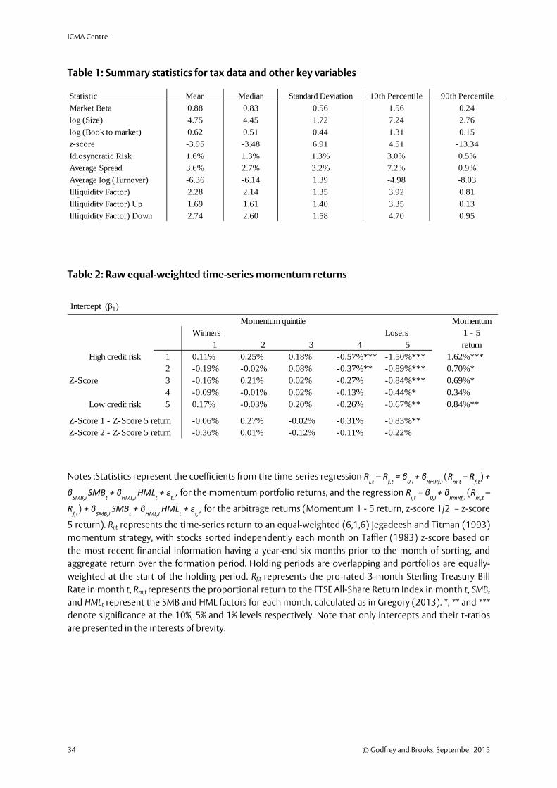
ICMA Centre
34 © Godfrey and Brooks, September 2015
Table 1: Summary statistics for tax data and other key variables
Table 2: Raw equal-weighted time-series momentum returns
Notes :Statistics represent the coefficients from the time-series regression Ri,t
– Rf,t
= β0,I
+ βRmRf,i
(Rm,t
– Rf,t
) +
βSMB,i
SMBt + β
HML,i HML
t + ε
t,i, for the momentum portfolio returns, and the regression R
i,t = β
0,I + β
RmRf,i (R
m,t –
Rf,t
) + βSMB,i
SMBt + β
HML,i HML
t + ε
t,i, for the arbitrage returns (Momentum 1 - 5 return, z-score 1/2 – z-score
5 return). Ri,t represents the time-series return to an equal-weighted (6,1,6) Jegadeesh and Titman (1993) momentum strategy, with stocks sorted independently each month on Taffler (1983) z-score based on the most recent financial information having a year-end six months prior to the month of sorting, and aggregate return over the formation period. Holding periods are overlapping and portfolios are equally-weighted at the start of the holding period. Rf,t represents the pro-rated 3-month Sterling Treasury Bill Rate in month t, Rm,t represents the proportional return to the FTSE All-Share Return Index in month t, SMBt and HMLt represent the SMB and HML factors for each month, calculated as in Gregory (2013). *, ** and *** denote significance at the 10%, 5% and 1% levels respectively. Note that only intercepts and their t-ratios are presented in the interests of brevity.
Statistic Mean Median Standard Deviation 10th Percentile 90th PercentileMarket Beta 0.88 0.83 0.56 1.56 0.24log (Size) 4.75 4.45 1.72 7.24 2.76log (Book to market) 0.62 0.51 0.44 1.31 0.15z-score -3.95 -3.48 6.91 4.51 -13.34Idiosyncratic Risk 1.6% 1.3% 1.3% 3.0% 0.5%Average Spread 3.6% 2.7% 3.2% 7.2% 0.9%Average log (Turnover) -6.36 -6.14 1.39 -4.98 -8.03g ( Illiquidity Factor) 2.28 2.14 1.35 3.92 0.81g ( Illiquidity Factor) Up 1.69 1.61 1.40 3.35 0.13g ( Illiquidity Factor) Down 2.74 2.60 1.58 4.70 0.95
Momentum quintile MomentumWinners Losers 1 - 5
1 2 3 4 5 returnHigh credit risk 1 0.11% 0.25% 0.18% -0.57%*** -1.50%*** 1.62%***
2 -0.19% -0.02% 0.08% -0.37%** -0.89%*** 0.70%*Z-Score 3 -0.16% 0.21% 0.02% -0.27% -0.84%*** 0.69%*
4 -0.09% -0.01% 0.02% -0.13% -0.44%* 0.34%Low credit risk 5 0.17% -0.03% 0.20% -0.26% -0.67%** 0.84%**
Z-Score 1 - Z-Score 5 return -0.06% 0.27% -0.02% -0.31% -0.83%**Z-Score 2 - Z-Score 5 return -0.36% 0.01% -0.12% -0.11% -0.22%
Intercept (β1)
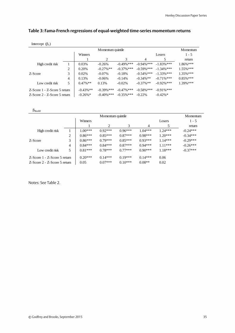
Henley Discussion Paper Series
© Godfrey and Brooks, September 2015 35
Table 3: Fama-French regressions of equal-weighted time-series momentum returns
Notes: See Table 2.
Momentum quintile MomentumWinners Losers 1 - 5
1 2 3 4 5 returnHigh credit risk 1 0.03% -0.26% -0.49%*** -0.94%*** -1.83%*** 1.86%***
2 0.20% -0.27%** -0.37%*** -0.59%*** -1.34%*** 1.55%***Z-Score 3 0.02% -0.07% -0.18% -0.54%*** -1.33%*** 1.35%***
4 0.13% -0.06% -0.14% -0.34%** -0.71%*** 0.85%***Low credit risk 5 0.47%** 0.13% -0.02% -0.37%** -0.92%*** 1.39%***
Z-Score 1 - Z-Score 5 return -0.43%** -0.39%*** -0.47%*** -0.58%*** -0.91%***Z-Score 2 - Z-Score 5 return -0.26%* -0.40%*** -0.35%*** -0.22% -0.42%*
Intercept (β1)
Momentum quintile MomentumWinners Losers 1 - 5
1 2 3 4 5 returnHigh credit risk 1 1.00*** 0.92*** 0.96*** 1.04*** 1.24*** -0.24***
2 0.86*** 0.85*** 0.87*** 0.98*** 1.20*** -0.34***Z-Score 3 0.86*** 0.79*** 0.85*** 0.93*** 1.14*** -0.29***
4 0.84*** 0.84*** 0.87*** 0.94*** 1.11*** -0.26***Low credit risk 5 0.81*** 0.78*** 0.77*** 0.90*** 1.18*** -0.37***
Z-Score 1 - Z-Score 5 return 0.20*** 0.14*** 0.19*** 0.14*** 0.06Z-Score 2 - Z-Score 5 return 0.05 0.07*** 0.10*** 0.08** 0.02
βRmRf
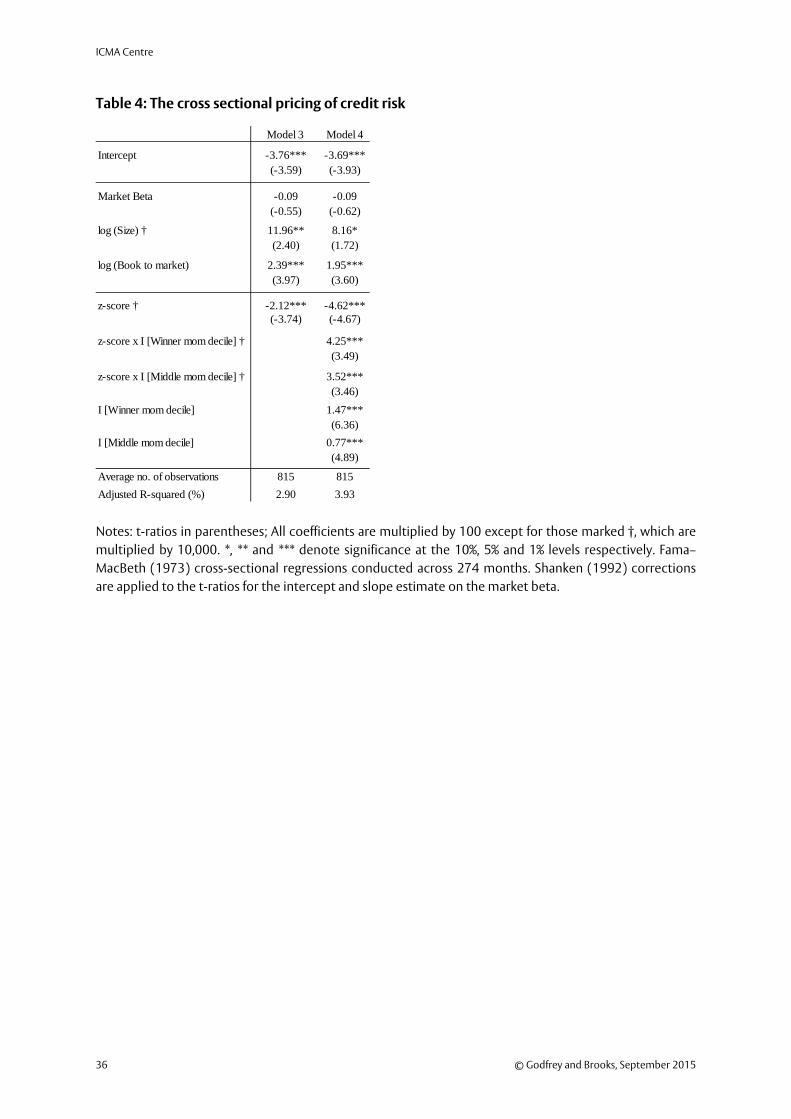
ICMA Centre
36 © Godfrey and Brooks, September 2015
Table 4: The cross sectional pricing of credit risk
Notes: t-ratios in parentheses; All coefficients are multiplied by 100 except for those marked †, which are multiplied by 10,000. *, ** and *** denote significance at the 10%, 5% and 1% levels respectively. Fama–MacBeth (1973) cross-sectional regressions conducted across 274 months. Shanken (1992) corrections are applied to the t-ratios for the intercept and slope estimate on the market beta.
Model 3 Model 4
Intercept -3.76*** -3.69***(-3.59) (-3.93)
Market Beta -0.09 -0.09(-0.55) (-0.62)
log (Size) † 11.96** 8.16*(2.40) (1.72)
log (Book to market) 2.39*** 1.95***(3.97) (3.60)
z-score † -2.12*** -4.62***(-3.74) (-4.67)
z-score x I [Winner mom decile] † 4.25***(3.49)
z-score x I [Middle mom decile] † 3.52***(3.46)
I [Winner mom decile] 1.47***(6.36)
I [Middle mom decile] 0.77***(4.89)
Average no. of observations 815 815Adjusted R-squared (%) 2.90 3.93
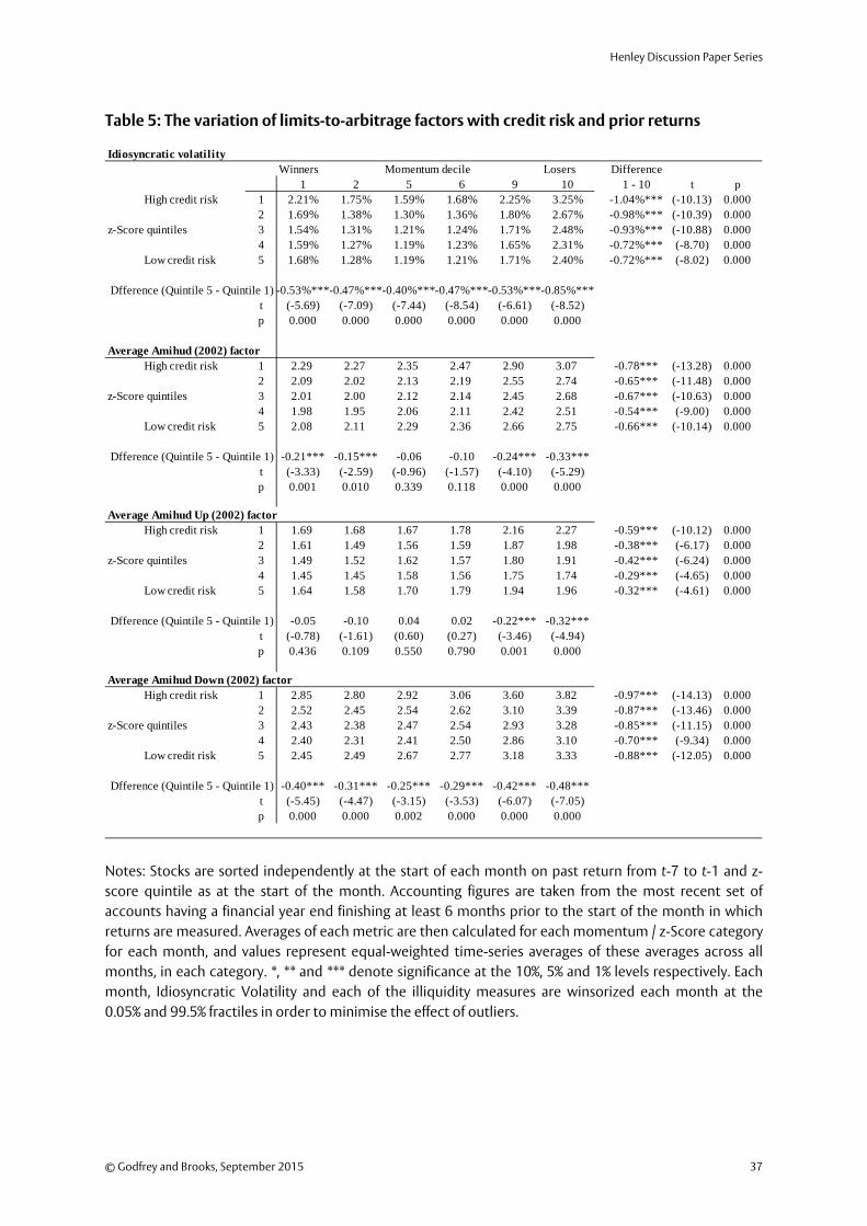
Henley Discussion Paper Series
© Godfrey and Brooks, September 2015 37
Table 5: The variation of limits-to-arbitrage factors with credit risk and prior returns
Notes: Stocks are sorted independently at the start of each month on past return from t-7 to t-1 and z-score quintile as at the start of the month. Accounting figures are taken from the most recent set of accounts having a financial year end finishing at least 6 months prior to the start of the month in which returns are measured. Averages of each metric are then calculated for each momentum / z-Score category for each month, and values represent equal-weighted time-series averages of these averages across all months, in each category. *, ** and *** denote significance at the 10%, 5% and 1% levels respectively. Each month, Idiosyncratic Volatility and each of the illiquidity measures are winsorized each month at the 0.05% and 99.5% fractiles in order to minimise the effect of outliers.
Idiosyncratic volatilityWinners Momentum decile Losers Difference
1 2 5 6 9 10 1 - 10 t pHigh credit risk 1 2.21% 1.75% 1.59% 1.68% 2.25% 3.25% -1.04%*** (-10.13) 0.000
2 1.69% 1.38% 1.30% 1.36% 1.80% 2.67% -0.98%*** (-10.39) 0.000z-Score quintiles 3 1.54% 1.31% 1.21% 1.24% 1.71% 2.48% -0.93%*** (-10.88) 0.000
4 1.59% 1.27% 1.19% 1.23% 1.65% 2.31% -0.72%*** (-8.70) 0.000Low credit risk 5 1.68% 1.28% 1.19% 1.21% 1.71% 2.40% -0.72%*** (-8.02) 0.000
Dfference (Quintile 5 - Quintile 1) -0.53%***-0.47%***-0.40%***-0.47%***-0.53%***-0.85%***t (-5.69) (-7.09) (-7.44) (-8.54) (-6.61) (-8.52)p 0.000 0.000 0.000 0.000 0.000 0.000
Average Amihud (2002) factor High credit risk 1 2.29 2.27 2.35 2.47 2.90 3.07 -0.78*** (-13.28) 0.000
2 2.09 2.02 2.13 2.19 2.55 2.74 -0.65*** (-11.48) 0.000z-Score quintiles 3 2.01 2.00 2.12 2.14 2.45 2.68 -0.67*** (-10.63) 0.000
4 1.98 1.95 2.06 2.11 2.42 2.51 -0.54*** (-9.00) 0.000Low credit risk 5 2.08 2.11 2.29 2.36 2.66 2.75 -0.66*** (-10.14) 0.000
Dfference (Quintile 5 - Quintile 1) -0.21*** -0.15*** -0.06 -0.10 -0.24*** -0.33***t (-3.33) (-2.59) (-0.96) (-1.57) (-4.10) (-5.29)p 0.001 0.010 0.339 0.118 0.000 0.000
Average Amihud Up (2002) factor High credit risk 1 1.69 1.68 1.67 1.78 2.16 2.27 -0.59*** (-10.12) 0.000
2 1.61 1.49 1.56 1.59 1.87 1.98 -0.38*** (-6.17) 0.000z-Score quintiles 3 1.49 1.52 1.62 1.57 1.80 1.91 -0.42*** (-6.24) 0.000
4 1.45 1.45 1.58 1.56 1.75 1.74 -0.29*** (-4.65) 0.000Low credit risk 5 1.64 1.58 1.70 1.79 1.94 1.96 -0.32*** (-4.61) 0.000
Dfference (Quintile 5 - Quintile 1) -0.05 -0.10 0.04 0.02 -0.22*** -0.32***t (-0.78) (-1.61) (0.60) (0.27) (-3.46) (-4.94)p 0.436 0.109 0.550 0.790 0.001 0.000
Average Amihud Down (2002) factor High credit risk 1 2.85 2.80 2.92 3.06 3.60 3.82 -0.97*** (-14.13) 0.000
2 2.52 2.45 2.54 2.62 3.10 3.39 -0.87*** (-13.46) 0.000z-Score quintiles 3 2.43 2.38 2.47 2.54 2.93 3.28 -0.85*** (-11.15) 0.000
4 2.40 2.31 2.41 2.50 2.86 3.10 -0.70*** (-9.34) 0.000Low credit risk 5 2.45 2.49 2.67 2.77 3.18 3.33 -0.88*** (-12.05) 0.000
Dfference (Quintile 5 - Quintile 1) -0.40*** -0.31*** -0.25*** -0.29*** -0.42*** -0.48***t (-5.45) (-4.47) (-3.15) (-3.53) (-6.07) (-7.05)p 0.000 0.000 0.002 0.000 0.000 0.000
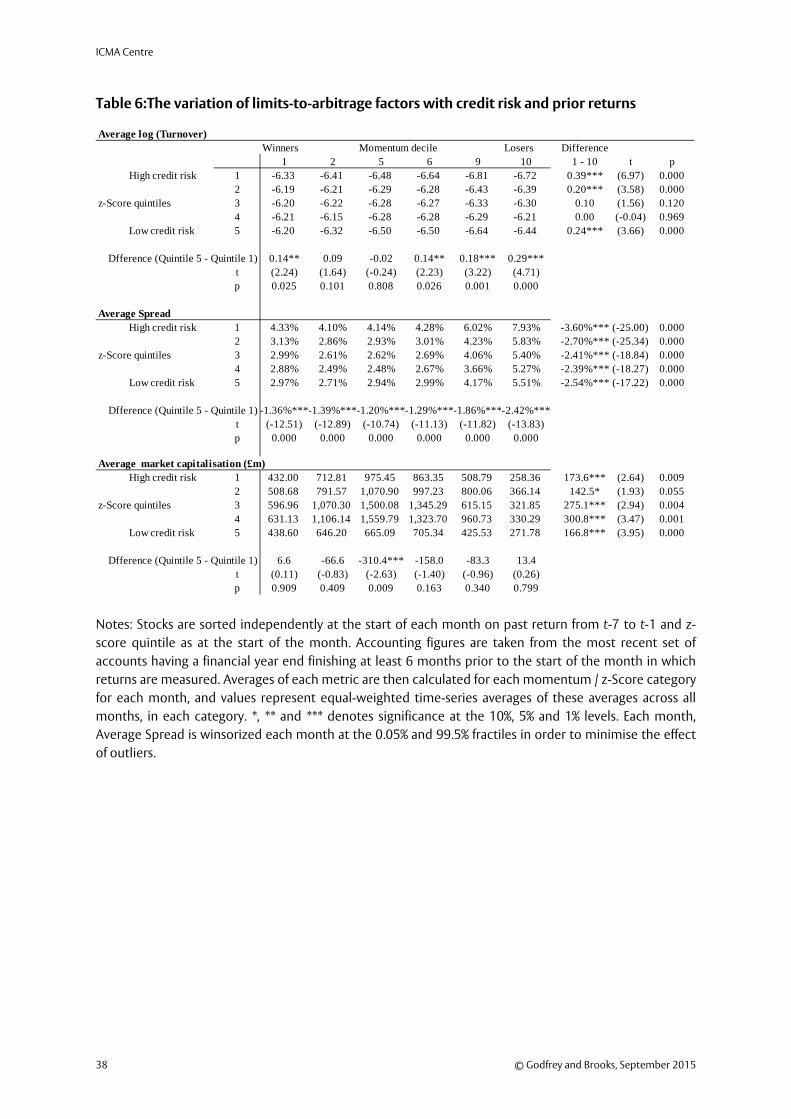
ICMA Centre
38 © Godfrey and Brooks, September 2015
Table 6:The variation of limits-to-arbitrage factors with credit risk and prior returns
Notes: Stocks are sorted independently at the start of each month on past return from t-7 to t-1 and z-score quintile as at the start of the month. Accounting figures are taken from the most recent set of accounts having a financial year end finishing at least 6 months prior to the start of the month in which returns are measured. Averages of each metric are then calculated for each momentum / z-Score category for each month, and values represent equal-weighted time-series averages of these averages across all months, in each category. *, ** and *** denotes significance at the 10%, 5% and 1% levels. Each month, Average Spread is winsorized each month at the 0.05% and 99.5% fractiles in order to minimise the effect of outliers.
Average log (Turnover) Winners Momentum decile Losers Difference
1 2 5 6 9 10 1 - 10 t pHigh credit risk 1 -6.33 -6.41 -6.48 -6.64 -6.81 -6.72 0.39*** (6.97) 0.000
2 -6.19 -6.21 -6.29 -6.28 -6.43 -6.39 0.20*** (3.58) 0.000z-Score quintiles 3 -6.20 -6.22 -6.28 -6.27 -6.33 -6.30 0.10 (1.56) 0.120
4 -6.21 -6.15 -6.28 -6.28 -6.29 -6.21 0.00 (-0.04) 0.969Low credit risk 5 -6.20 -6.32 -6.50 -6.50 -6.64 -6.44 0.24*** (3.66) 0.000
Dfference (Quintile 5 - Quintile 1) 0.14** 0.09 -0.02 0.14** 0.18*** 0.29***t (2.24) (1.64) (-0.24) (2.23) (3.22) (4.71)p 0.025 0.101 0.808 0.026 0.001 0.000
Average SpreadHigh credit risk 1 4.33% 4.10% 4.14% 4.28% 6.02% 7.93% -3.60%*** (-25.00) 0.000
2 3.13% 2.86% 2.93% 3.01% 4.23% 5.83% -2.70%*** (-25.34) 0.000z-Score quintiles 3 2.99% 2.61% 2.62% 2.69% 4.06% 5.40% -2.41%*** (-18.84) 0.000
4 2.88% 2.49% 2.48% 2.67% 3.66% 5.27% -2.39%*** (-18.27) 0.000Low credit risk 5 2.97% 2.71% 2.94% 2.99% 4.17% 5.51% -2.54%*** (-17.22) 0.000
Dfference (Quintile 5 - Quintile 1) -1.36%***-1.39%***-1.20%***-1.29%***-1.86%***-2.42%***t (-12.51) (-12.89) (-10.74) (-11.13) (-11.82) (-13.83)p 0.000 0.000 0.000 0.000 0.000 0.000
Average market capitalisation (£m) High credit risk 1 432.00 712.81 975.45 863.35 508.79 258.36 173.6*** (2.64) 0.009
2 508.68 791.57 1,070.90 997.23 800.06 366.14 142.5* (1.93) 0.055z-Score quintiles 3 596.96 1,070.30 1,500.08 1,345.29 615.15 321.85 275.1*** (2.94) 0.004
4 631.13 1,106.14 1,559.79 1,323.70 960.73 330.29 300.8*** (3.47) 0.001Low credit risk 5 438.60 646.20 665.09 705.34 425.53 271.78 166.8*** (3.95) 0.000
Dfference (Quintile 5 - Quintile 1) 6.6 -66.6 -310.4*** -158.0 -83.3 13.4t (0.11) (-0.83) (-2.63) (-1.40) (-0.96) (0.26)p 0.909 0.409 0.009 0.163 0.340 0.799
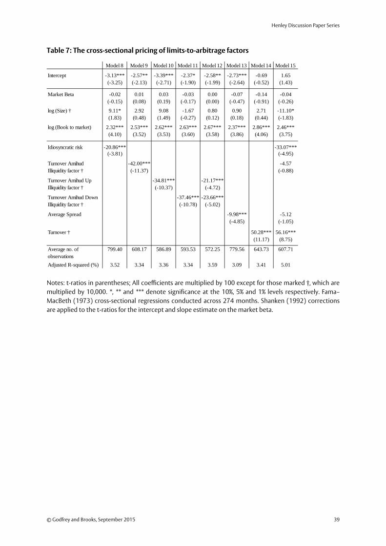
Henley Discussion Paper Series
© Godfrey and Brooks, September 2015 39
Table 7: The cross-sectional pricing of limits-to-arbitrage factors
Notes: t-ratios in parentheses; All coefficients are multiplied by 100 except for those marked †, which are multiplied by 10,000. *, ** and *** denote significance at the 10%, 5% and 1% levels respectively. Fama–MacBeth (1973) cross-sectional regressions conducted across 274 months. Shanken (1992) corrections are applied to the t-ratios for the intercept and slope estimate on the market beta.
Model 8 Model 9 Model 10 Model 11 Model 12 Model 13 Model 14 Model 15
Intercept -3.13*** -2.57** -3.39*** -2.37* -2.58** -2.73*** -0.69 1.65(-3.25) (-2.13) (-2.71) (-1.90) (-1.99) (-2.64) (-0.52) (1.43)
Market Beta -0.02 0.01 0.03 -0.03 0.00 -0.07 -0.14 -0.04(-0.15) (0.08) (0.19) (-0.17) (0.00) (-0.47) (-0.91) (-0.26)
log (Size) † 9.11* 2.92 9.08 -1.67 0.80 0.90 2.71 -11.10*(1.83) (0.48) (1.49) (-0.27) (0.12) (0.18) (0.44) (-1.83)
log (Book to market) 2.32*** 2.53*** 2.62*** 2.63*** 2.67*** 2.37*** 2.86*** 2.46***(4.10) (3.52) (3.53) (3.60) (3.58) (3.86) (4.06) (3.75)
-20.86*** -33.07***(-3.81) (-4.95)
-42.00*** -4.57(-11.37) (-0.88)
-34.81*** -21.17***(-10.37) (-4.72)
-37.46*** -23.66***(-10.78) (-5.02)
Average Spread -9.98*** -5.12(-4.85) (-1.05)
Turnover † 50.28*** 56.16***(11.17) (8.75)
Average no. of observations
799.40 608.17 586.89 593.53 572.25 779.56 643.73 607.71
Adjusted R-squared (%) 3.52 3.34 3.36 3.34 3.59 3.09 3.41 5.01
Idiosyncratic risk
Turnover Amihud Illiquidity factor †
Turnover Amihud Up Illiquidity factor †
Turnover Amihud Down Illiquidity factor †

ICMA Centre
40 © Godfrey and Brooks, September 2015
Table 8: Variation of the negative credit spread with limits-to-arbitrage factors
Notes: Risk-adjusted negative credit spread returns, by deciles of limits-to-arbitrage factors, after Ali et al (2003). Each month, stocks are sorted simultaneously into quintiles of credit risk and deciles of each limits-to-arbitrage factor, with Q1 (Q5) representing the quintile of highest (lowest) credit risk, and LTA1 (LTA10) representing the decile of highest (lowest) limits-to-arbitrage factor, i.e. highest (lowest) idiosyncratic volatility, widest (narrowest) average spread, highest (lowest) unadjusted share price, highest (lowest) turnover, most illiquid (most liquid), and highest market value (smallest market value) stocks, respectively. Reported statistics for each LTA decile x represent the month-ahead return for the trading strategy which is long the Q1, LTAx portfolio and short the Q5, LTAx portfolio. LTA1 – LTA10 statistics represent the month-ahead trading strategy which is long (short) the Q1, LTA1 and Q5, LTA10 (Q1, LTA5 and Q5, LTA1) portfolios. t-statistics are in brackets. Accounting figures are taken from the most recent set of accounts having a financial year end finishing at least 6 months prior to the start of the month in which returns are measured. Portfolios are equal-weighted, in each category. *, ** and *** denote significance at the 10%, 5% and 1% levels respectively.
VariableIdiosyncratic
VolatilityAverage Spread
Unadjusted Price Turnover
Turnover Amihud Illiquidity Factor
Up Turnover Amihud Illiquidity Factor
Down Turnover Amihud Illiquidity Factor Size
LTA1 -0.68% -1.31%*** 0.09% 0.06% -1.20%** -0.85%* -1.25%** 0.05%(High) (-1.38) (-3.26) (0.29) (0.11) (-2.37) (-1.76) (-2.44) (0.18)
LTA2 -0.36% -0.37% -0.10% 0.28% -0.88%* -1.09%** -0.82% -0.32%(-0.92) (-0.88) (-0.35) (0.52) (-1.88) (-2.46) (-1.56) (-0.94)
LTA3 -0.36% -0.45% -0.21% -0.34% -0.26% -1.07%** 0.27% -0.13%(-1.03) (-1.17) (-0.65) (-0.75) (-0.55) (-2.16) (0.54) (-0.39)
LTA4 -0.38% -0.39% -0.26% -0.21% -0.77% -0.83% -0.49% -0.53%(-1.09) (-1.17) (-0.82) (-0.49) (-1.56) (-1.46) (-1.14) (-1.45)
LTA5 -0.66%** -0.44% -0.35% -0.38% -0.31% -1.19%** -0.33% -0.46%(-2.18) (-1.17) (-1.02) (-0.80) (-0.61) (-2.37) (-0.76) (-1.34)
LTA6 -0.37% -0.65%* -0.89%*** -0.68% -0.34% 0.27% -0.30% -0.63%*(-1.20) (-1.94) (-2.71) (-1.58) (-0.79) (0.53) (-0.61) (-1.77)
LTA7 -0.43% -0.27% -0.12% -0.42% -0.55% -0.60% 0.20% -1.07%***(-1.41) (-0.78) (-0.33) (-0.96) (-1.05) (-1.30) (0.37) (-2.75)
LTA8 -0.62%** 0.16% 0.18% -0.55% 0.14% -0.08% 0.13% -1.10%***(-2.04) (0.44) (0.50) (-1.16) (0.35) (-0.20) (0.28) (-2.95)
LTA9 -0.79%** -0.21% -0.46% -1.34%*** -0.24% 0.83%* -0.10% -0.22%(-2.37) (-0.55) (-1.30) (-2.92) (-0.60) (1.94) (-0.24) (-0.59)
LTA10 -0.58%* 0.07% -0.99%* -1.23%*** 0.48% -0.45% 0.43% -1.04%***(Low) (-1.95) (0.23) (-1.79) (-2.75) (1.07) (-0.94) (1.12) (-2.71)
LTA1 - LTA10 -0.10% -1.38%*** 1.07%* 1.13%* -1.53%** -0.21% -1.46%** 1.09%**(High - Low) (-0.20) (-2.75) (1.70) (1.96) (-2.35) (-0.32) (-2.53) (2.35)
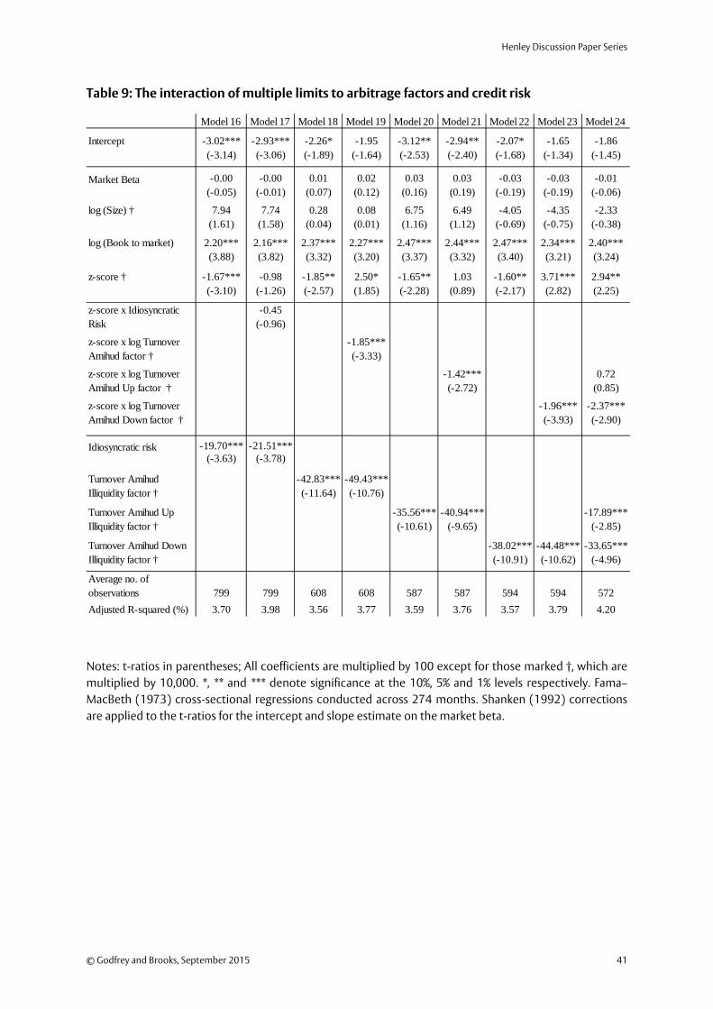
Henley Discussion Paper Series
© Godfrey and Brooks, September 2015 41
Table 9: The interaction of multiple limits to arbitrage factors and credit risk
Notes: t-ratios in parentheses; All coefficients are multiplied by 100 except for those marked †, which are multiplied by 10,000. *, ** and *** denote significance at the 10%, 5% and 1% levels respectively. Fama–MacBeth (1973) cross-sectional regressions conducted across 274 months. Shanken (1992) corrections are applied to the t-ratios for the intercept and slope estimate on the market beta.
Model 16 Model 17 Model 18 Model 19 Model 20 Model 21 Model 22 Model 23 Model 24
Intercept -3.02*** -2.93*** -2.26* -1.95 -3.12** -2.94** -2.07* -1.65 -1.86(-3.14) (-3.06) (-1.89) (-1.64) (-2.53) (-2.40) (-1.68) (-1.34) (-1.45)
Market Beta -0.00 -0.00 0.01 0.02 0.03 0.03 -0.03 -0.03 -0.01(-0.05) (-0.01) (0.07) (0.12) (0.16) (0.19) (-0.19) (-0.19) (-0.06)
log (Size) † 7.94 7.74 0.28 0.08 6.75 6.49 -4.05 -4.35 -2.33(1.61) (1.58) (0.04) (0.01) (1.16) (1.12) (-0.69) (-0.75) (-0.38)
log (Book to market) 2.20*** 2.16*** 2.37*** 2.27*** 2.47*** 2.44*** 2.47*** 2.34*** 2.40***(3.88) (3.82) (3.32) (3.20) (3.37) (3.32) (3.40) (3.21) (3.24)
z-score † -1.67*** -0.98 -1.85** 2.50* -1.65** 1.03 -1.60** 3.71*** 2.94**(-3.10) (-1.26) (-2.57) (1.85) (-2.28) (0.89) (-2.17) (2.82) (2.25)
-0.45(-0.96)
-1.85***(-3.33)
-1.42*** 0.72(-2.72) (0.85)
-1.96*** -2.37***(-3.93) (-2.90)
-19.70*** -21.51***(-3.63) (-3.78)
-42.83*** -49.43***(-11.64) (-10.76)
-35.56*** -40.94*** -17.89***(-10.61) (-9.65) (-2.85)
-38.02*** -44.48*** -33.65***(-10.91) (-10.62) (-4.96)
Average no. of observations 799 799 608 608 587 587 594 594 572Adjusted R-squared (%) 3.70 3.98 3.56 3.77 3.59 3.76 3.57 3.79 4.20
Idiosyncratic risk
Turnover Amihud Illiquidity factor †
Turnover Amihud Down Illiquidity factor †
Turnover Amihud Up Illiquidity factor †
z-score x Idiosyncratic Risk
z-score x log Turnover Amihud factor †
z-score x log Turnover Amihud Up factor †
z-score x log Turnover Amihud Down factor †

ICMA Centre
42 © Godfrey and Brooks, September 2015
Table 10: The interaction of multiple limits to arbitrage factors and credit risk
Notes: t-ratios in parentheses; All coefficients are multiplied by 100 except for those marked †, which are multiplied by 10,000. *, ** and *** denote significance at the 10%, 5% and 1% levels respectively. Fama–MacBeth (1973) cross-sectional regressions conducted across 274 months. Shanken (1992) corrections are applied to the t-ratios for the intercept and slope estimate on the market beta.
Model 25 Model 26 Model 27 Model 28 Model 29 Model 30 Model 31 Model 32 Model 33
Intercept -2.61** -2.49** -0.34 -0.02 1.88 1.85 2.13* 2.44** 2.17*(-2.54) (-2.41) (-0.26) (-0.01) (1.55) (1.61) (1.84) (2.10) (1.87)
Market Beta -0.06 -0.06 -0.14 -0.13 -0.03 -0.04 -0.05 -0.06 -0.05(-0.40) (-0.42) (-0.90) (-0.85) (-0.20) (-0.28) (-0.41) (-0.47) (-0.41)
log (Size) † -0.12 -0.31 0.19 0.46 -12.31** -12.47** -14.52*** -16.32*** -14.67***(-0.02) (-0.06) (0.03) (0.07) (-2.04) (-2.07) (-2.74) (-3.08) (-2.62)
log (Book to market) 2.26*** 2.20*** 2.67*** 2.59*** 2.40*** 2.34*** 2.37*** 2.26*** 2.38***(3.70) (3.58) (3.81) (3.70) (3.47) (3.54) (3.55) (3.37) (3.58)
z-score † -1.46** -0.86 -2.08*** 5.71** -1.04 -1.23* -1.04* -0.82 -1.02*(-2.53) (-1.13) (-2.96) (2.11) (-1.52) (-1.87) (-1.67) (-1.28) (-1.67)
-0.16(-0.84)
1.18***(2.81)
-34.20*** -32.65*** -32.24*** -32.70*** -32.04***(-5.02) (-4.91) (-5.51) (-5.29) (-5.32)
-5.40 -2.78(-1.04) (-0.56)
-2.69(-0.64)
1.16(0.22)
-9.63*** -10.33*** -4.54 -4.32 -2.79(-4.77) (-4.66) (-0.85) (-0.88) (-0.01)
Turnover † 50.91*** 54.31*** 59.31*** 56.24*** 59.38*** 59.44*** 59.91***(11.38) (11.36) (8.55) (8.78) (14.39) (9.73) (14.87)
Average no. of observations
780 780 644 644 572 608 676 647 675
Adjusted R-squared (%)
3.29 3.51 3.62 3.72 5.38 5.18 4.23 4.44 4.50
Idiosyncratic risk
Turnover Amihud Illiquidity factor †
Turnover Amihud Up Illiquidity factor †
Turnover Amihud Down Illiquidity factor
Average Spread
z-score x Average Spread
z-score x log Turnover †

Henley Discussion Paper Series
© Godfrey and Brooks, September 2015 43
Appendix: Data Handling Approach
Filtering methodology
The analyses in this paper are principally either double-sorts, in which one axis of the sort is a
ranking on prior returns over a holding period, or else are cross-sectional regressions. In order to
be included in the dataset at the start of the holding period, in the case of double-sorts, or at the
start of the month in which returns are measured, in the case of cross-sectional regression, a
company must have:
• A market capitalisation of at least £10m, in order to select only those stocks in which a
realistic degree of liquidity is present;
• Been listed for at least 24 months, in order to enable 24-month pre-ranking market betas to
be calculated for each stock;
• An actively-quoted mid-price available for at least 10 days in the previous month before the
start of the respective period;
• Valid PI (price index), RI (return index) and MV (market cap) information in Datastream at the
start of the respective period;
• An industry code other than finance stocks, real estate investment trusts or real estate
holding companies, or an indeterminate industry classification (Datastream industry level 2
codes FINAN or NA);
• Valid accounting information at the start of the respective period to calculate the Taffler z-
score (defined in the following section), namely, Profit before Tax, Total Liabilities, Current
Liabilities, Total Assets, Current Assets, Cash, Sales and Depreciation. In order to guarantee
non-infinite values of the z-score, Current Liabilities, Total Liabilities, Total Assets and (Sales -
Profit before Tax - Depreciation) must be all nonzero. Additionally, in order to exclude Cash
Shells, equities representing investment vehicles and dormant companies, the value of Sales
must be present and nonzero;
• Valid accounting information at the start of the respective period to calculate Book-to-
Market values, namely, Common Equity and a nonzero Market Value on the latest trading
date immediately prior to the financial year end.
ICMA Centre
44 © Godfrey and Brooks, September 2015
Delisting methodology
Delisting information is taken from the London Share Price Database (LSPD), or where
information is unavailable, from Regulatory News Service news searches collated by hand.
Where a stock is delisted through failure, it is assigned a -100% return upon delisting, otherwise
we assume that the investor receives its full value, as at the date of delisting. Although the LSPD
records the month from which a stock is no longer quoted, we prefer to use the last active date
of trading as the date on which a stock exits the sample. There is normally is a delay of some
weeks between the last day of active trading for practical purposes and the point at which a
stock is formally delisted, and this is caused sometimes by the issuer or a bidder announcing the
possibility of delisting, and at others by unilateral suspension of the shares by the Financial
Conduct Authority.
Sorting methodology
Studies involving US data generally presume a December 31 financial year-end for the vast
majority of companies, and allow six months for the publication of accounts, and so match
monthly returns from July of year t to June of year t+1 with accounts whose financial year ends
are in December of year t–1. As regards UK studies, Dimson et al. (2003) follow the standard US
practice, while Agarwal and Taffler (2008), Agarwal and Poshakwale (2010) and Gregory et al.
(2013) sort stocks from 1 October each year on the basis of accounts filings having financial year
end dates of 31 March in the same year, at the latest.
However, the distribution of year ends in the present sample is spread over the year, so that this
latter sorting methodology would be three months late in using accounts information relating
to the 41% of stocks with December financial year ends; the conventional method for US stocks
would not be any more timely in using accounts information, as it would be nine months late in
using accounts information relating to the 20% of stocks with March financial year ends. Since
both yearly sorting methods employed in the literature have drawbacks, we sort stocks on a
rolling monthly basis, taking at each month the most recent accounts with a financial year end at
least six months prior to the month in which sorting is taking place. A firm that has a financial
year end of December will then have the monthly returns of July of year t to June of year t+1
matched with the accounts data for the financial year ending December of year t–1, while a firm
having a financial year end in March will have the monthly returns of October of year t to
September of year t+1 matched with the accounts data for the financial year ending March of
year t.
Henley Discussion Paper Series
© Godfrey and Brooks, September 2015 45
Data cleaning and winsorization methodology
Comparison of Datastream with other datasets has given rise to warnings that care ought to be
taken when calculating returns from Datastream to avoid spurious results arising from data
errors, and to avoid incorrect sample inferences being drawn from a handful of extreme returns.
The general practice in cleaning Datastream data is therefore to exclude small stocks by some
criterion (Hong et al., 2003), and to winsorize returns to avoid spurious inferences being drawn
from data errors (Chui et al., 2010; Ince and Porter, 2006; Sudarsanam and Mahate, 2003). For
the present sample, we elect not to exclude stocks on the basis of falling below a certain
percentile of market capitalisation, since this introduces the risk that more small, illiquid stocks
will be admitted to the sample simply because there were more small stocks listed at that point
in time. Instead, for the present paper, we exclude all stocks from the dataset which have a
market capitalisation of less than £10m at the start of the month over which dependent variable
returns are taken – this is a more severe criterion than in Hong et al. (2003), since it excludes on
average 22.6% of the sample which would have otherwise been admitted had this rule not been
applied.
Regarding winsorization on the downside, our delisting procedure generates monthly returns of
-100% when a stock delists due to bankruptcy or distress, and these cases have either been
designated from LSPD delisting data or coded by hand using news searches, so we treat these as
reliable. Though Ince and Porter (2006) find examples of monthly returns of 300% or more
which are reversed within the month, we find only three examples of monthly returns over 100%
which are reversed the next month, and each of these is explicable by relation to extant
company news rather than data errors. The remaining very small proportion of returns (0.08% of
sample firm-months) which have monthly returns over 100% reflect real permanent changes in
company value, and so we elect instead to winsorize each month on the upside at 200%, to avoid
undue influence being exerted on the results by the handful of cases (20 firm-months,
representing 0.008% of sample firm-months) which have monthly returns in excess of that limit.
We also winsorize some independent variables: we follow Fama and French (1992), Chordia and
Shivakumar (2006), Fu (2009), Chordia et al. (2009), Chou et al. (2010) and Brennan et al.
(2013) in winsorizing the log (book to market) variable to avoid placing undue emphasis on
outliers. We follow the example of Dichev (1998), who winsorizes the Ohlson (1980) O-Score
and the Altman (1968) Z-Score measures of relative distress, in winsorizing values of the Taffler
(1983) z-score; both are winsorized each month at the 2.5% and 97.5% fractiles. Following
Brennan et al. (2013), we winsorize the bid-ask spread, and following Fu (2009), we winsorize

ICMA Centre
46 © Godfrey and Brooks, September 2015
idiosyncratic volatility each month at the 0.5% and 99.5% fractiles. The Turnover Amihud
statistics and bid-ask spread are winsorized each month at the 0.5% and 99.5% fractiles.
Calculation of Fama-French factors
SMB and HML factors for each day are calculated by using the methodology and breakpoints as
in Gregory et al. (2013).
Pairwise correlation statistics are calculated using the analytics in RExcel (Baier and Neuwirth,
2007).
Henley Discussion Paper Series
© Godfrey and Brooks, September 2015 47
References
Agarwal, V., Bauer, J., 2014. Distress Risk and Stock Returns: The neglected Profitability Effect? Paper presented at the 2014 FMA Annual Meeting, Nashville, TN, October 15 - 18 [WWW Document]. URL http://www.fma.org/Nashville/Papers/Distress_and_Returns_Full.pdf (accessed 5.16.14).
Agarwal, V., Poshakwale, S., 2010. Size and book-to-market anomalies and omitted leverage risk. European Journal of Finance 16, 263–279. doi:10.1080/13518470903314402
Agarwal, V., Taffler, R., 2008. Does Financial Distress Risk Drive the Momentum Anomaly? Financial Management 37, 461–484.
Ali, A., Hwang, L.-S., Trombley, M.A., 2003. Arbitrage risk and the book-to-market anomaly. Journal of Financial Economics 69, 355–373. doi:10.1016/S0304-405X(03)00116-8
Ali, A., Trombley, M.A., 2006. Short Sales Constraints and Momentum in Stock Returns. Journal of Business Finance & Accounting 33, 587–615. doi:10.1111/j.1468-5957.2006.00616.x
Altman, E.I., 1968. Financial Ratios, Discriminant Analysis and the Prediction of Corporate Bankruptcy. Journal of Finance 23, 589–609. doi:10.2307/2978933
Amihud, Y., 2002. Illiquidity and stock returns: cross-section and time-series effects. Journal of Financial Markets 5, 31–56. doi:10.1016/S1386-4181(01)00024-6
Amihud, Y., Mendelson, H., 1986. Asset pricing and the bid-ask spread. Journal of Financial Economics 17, 223–249. doi:10.1016/0304-405X(86)90065-6
Ang, A., Hodrick, R.J., Xing, Y., Zhang, X., 2009. High idiosyncratic volatility and low returns: International and further U.S. evidence. Journal of Financial Economics 91, 1–23. doi:10.1016/j.jfineco.2007.12.005
Ang, A., Hodrick, R.J., Xing, Y., Zhang, X., 2006. The Cross-Section of Volatility and Expected Returns. Journal of Finance 61, 259–299.
Arena, M.P., Haggard, K.S., Yan, X. (Sterling), 2008. Price Momentum and Idiosyncratic Volatility. Financial Review 43, 159–190. doi:10.1111/j.1540-6288.2008.00190.x
Au, A.S., Doukas, J.A., Onayev, Z., 2009. Daily short interest, idiosyncratic risk, and stock returns. Journal of Financial Markets 12, 290–316. doi:10.1016/j.finmar.2008.09.001
Avramov, D., Cederburg, S., Hore, S., 2011. Cross-Sectional Asset Pricing Puzzles: A Long-Run Perspective [WWW Document]. URL http://papers.ssrn.com/abstract=1314869 (accessed 8.14.14).
Avramov, D., Chordia, T., Jostova, G., Philipov, A., 2009. Credit ratings and the cross-section of stock returns. Journal of Financial Markets 12, 469–499. doi:10.1016/j.finmar.2009.01.005
Avramov, D., Chordia, T., Jostova, G., Philipov, A., 2007. Momentum and Credit Rating. Journal of Finance 62, 2503–2520. doi:10.1111/j.1540-6261.2007.01282.x
ICMA Centre
48 © Godfrey and Brooks, September 2015
Baier, T., Neuwirth, E., 2007. Excel :: COM :: R. Computational Statistics 22, 91–108. doi:10.1007/s00180-007-0023-6
Bali, T.G., Cakici, N., 2008. Idiosyncratic Volatility and the Cross Section of Expected Returns. Journal of Financial & Quantitative Analysis 43, 29–58.
Barber, B.M., Odean, T., 2000. Trading Is Hazardous to Your Wealth: The Common Stock Investment Performance of Individual Investors. Journal of Finance 55, 773–806.
Barber, B.M., Yi-Tsung Lee, Yu-Jane Liu, Odean, T., 2007. Is the Aggregate Investor Reluctant to Realise Losses? Evidence from Taiwan. European Financial Management 13, 423–447. doi:10.1111/j.1468-036X.2007.00367.x
Blazy, R., Chopard, B., Nigam, N., 2013. Building legal indexes to explain recovery rates: An analysis of the French and English bankruptcy codes. Journal of Banking & Finance 37, 1936–1959. doi:10.1016/j.jbankfin.2012.10.024
Brennan, M., Huh, S.-W., Subrahmanyam, A., 2013. An Analysis of the Amihud Illiquidity Premium. Review of Asset Pricing Studies 3, 133–176. doi:10.1093/rapstu/ras017
Brennan, M.J., Subrahmanyam, A., 1996. Market microstructure and asset pricing: On the compensation for illiquidity in stock returns. Journal of Financial Economics 41, 441–464. doi:10.1016/0304-405X(95)00870-K
Campbell, J.Y., Hilscher, J., Szilagyi, J., 2008. In Search of Distress Risk. Journal of Finance 63, 2899–2939. doi:10.1111/j.1540-6261.2008.01416.x
Chava, S., Purnanandam, A., 2010. Is Default Risk Negatively Related to Stock Returns? Review of Financial Studies 23, 2523–2559. doi:10.1093/rfs/hhp107
Chen, J., Chollete, L., Ray, R., 2010. Financial distress and idiosyncratic volatility: An empirical investigation. Journal of Financial Markets 13, 249–267. doi:10.1016/j.finmar.2009.10.003
Choi, J., Kim, Y., 2015. Anomalies and Market (Dis)Integration [WWW Document]. URL http://papers.ssrn.com/abstract=2412086 (accessed 5.25.15).
Chordia, T., Huh, S.-W., Subrahmanyam, A., 2009. Theory-Based Illiquidity and Asset Pricing. Review of Financial Studies 22, 3629–3668. doi:10.1093/rfs/hhn121
Chordia, T., Shivakumar, L., 2006. Earnings and price momentum. Journal of Financial Economics 80, 627–656. doi:10.1016/j.jfineco.2005.05.005
Chou, P.-H., Ko, K.-C., Lin, S.-J., 2010. Do relative leverage and relative distress really explain size and book-to-market anomalies? Journal of Financial Markets 13, 77–100. doi:10.1016/j.finmar.2009.07.007
Chua, C.T., Goh, J., Zhang, Z., 2010. Expected Volatility, Unexpected Volatility, and the Cross-Section of Stock Returns. Journal of Financial Research 33, 103–123. doi:10.1111/j.1475-6803.2010.01264.x
Chui, A.C. w, Titman, S., Wei, K. c. J., 2010. Individualism and Momentum around the World. Journal of Finance 65, 361–392. doi:10.1111/j.1540-6261.2009.01532.x
Henley Discussion Paper Series
© Godfrey and Brooks, September 2015 49
Davydenko, S.A., Franks, J.R., 2008. Do Bankruptcy Codes Matter? A Study of Defaults in France, Germany, and the U.K. Journal of Finance 63, 565–608.
Da, Z., Gao, P., 2010. Clientele Change, Liquidity Shock, and the Return on Financially Distressed Stocks. Journal of Financial & Quantitative Analysis 45, 27–48.
Dhar, R., Ning Zhu, 2006. Up Close and Personal: Investor Sophistication and the Disposition Effect. Management Science 52, 726–740. doi:10.1287/mnsc.1040.0473
Dichev, I.D., 1998. Is the Risk of Bankruptcy a Systematic Risk? Journal of Finance 53, 1131–1147.
Dimson, E., Nagel, S., Quigley, G., 2003. Capturing the Value Premium in the United Kingdom. Financial Analysts Journal 59, 35–45.
Duan, Y., Hu, G., McLean, R.D., 2010. Costly arbitrage and idiosyncratic risk: Evidence from short sellers. Journal of Financial Intermediation 19, 564–579. doi:10.1016/j.jfi.2009.06.003
Eisdorfer, A., Goyal, A., Zhdanov, A., 2013. Distress Anomaly and Shareholder Risk: International Evidence [WWW Document]. URL http://papers.ssrn.com/abstract=2267611 (accessed 5.25.15).
Eisdorfer, A., Goyal, A., Zhdanov, A., 2012. Misvaluation and Return Anomalies in Distress Stocks [WWW Document]. URL http://papers.ssrn.com/abstract=2023778 (accessed 3.20.13).
Eleswarapu, V.R., Reinganum, M.R., 1993. The seasonal behavior of the liquidity premium in asset pricing. Journal of Financial Economics 34, 373–386. doi:10.1016/0304-405X(93)90032-7
Fama, E.F., French, K.R., 1996. The CAPM is Wanted, Dead or Alive. Journal of Finance 51, 1947–1958. doi:10.2307/2329545
Fama, E.F., French, K.R., 1993. Common risk factors in the returns on stocks and bonds. Journal of Financial Economics 33, 3–56. doi:10.1016/0304-405X(93)90023-5
Fama, E.F., French, K.R., 1992. The Cross-Section of Expected Stock Returns. Journal of Finance 47, 427–465. doi:10.2307/2329112
Fama, E.F., MacBeth, J.D., 1973. Risk, return, and equilibrium: Empirical tests. Journal of Political Economy 607–636.
Ferguson, M.F., Shockley, R.L., 2003. Equilibrium “Anomalies.” Journal of Finance 58, 2549–2580. doi:10.1046/j.1540-6261.2003.00615.x
Finn, M.T., Fuller, R.J., King, J.L., 1999. Equity Mispricing: It’s Mostly on the Short Side. Financial Analysts Journal 55, 117.
Franks, J., Sussman, O., 2005. Financial Distress and Bank Restructuring of Small to Medium Size UK Companies. Review of Finance 9, 65–96. doi:10.1007/s10679-005-2988-8
Friewald, N., Wagner, C., Zechner, J., 2014. The Cross-Section of Credit Risk Premia and Equity Returns. The Journal of Finance 69, 2419–2469. doi:10.1111/jofi.12143
Fu, F., 2009. Idiosyncratic risk and the cross-section of expected stock returns. Journal of Financial Economics 91, 24–37. doi:10.1016/j.jfineco.2008.02.003
ICMA Centre
50 © Godfrey and Brooks, September 2015
Gao, P., Parsons, C.A., Shen, J., 2013. The Global Relation between Financial Distress and Equity Returns [WWW Document]. URL http://papers.ssrn.com/abstract=2086475 (accessed 5.25.15).
Garlappi, L., Yan, H., 2011. Financial Distress and the Cross Section of Equity Returns. Journal of Finance 66, 789–822. doi:10.1111/j.1540-6261.2011.01652.x
George, T.J., Hwang, C.-Y., 2010. A resolution of the distress risk and leverage puzzles in the cross section of stock returns. Journal of Financial Economics 96, 56–79. doi:10.1016/j.jfineco.2009.11.003
Glosten, L.R., Harris, L.E., 1988. Estimating the components of the bid/ask spread. Journal of Financial Economics 21, 123–142. doi:10.1016/0304-405X(88)90034-7
Goetzmann, W.N., Massa, M., 2008. Disposition Matters: Volume, Volatility, and Price Impact of a Behavioral Bias. Journal of Portfolio Management 34, 103–125.
Gregory, A., Tharyan, R., Christidis, A., 2013. Constructing and Testing Alternative Versions of the Fama–French and Carhart Models in the UK. Journal of Business Finance & Accounting 40, 172–214. doi:10.1111/jbfa.12006
Griffin, J.M., Lemmon, M.L., 2002. Book–to–Market Equity, Distress Risk, and Stock Returns. Journal of Finance 57, 2317–2336. doi:10.1111/1540-6261.00497
Grinblatt, M., Keloharju, M., 2000. The investment behavior and performance of various investor types: a study of Finland’s unique data set. Journal of Financial Economics 55, 43–67. doi:10.1016/S0304-405X(99)00044-6
Gromb, D., Vayanos, D., 2010. Limits of Arbitrage: The State of the Theory, INSEAD Working Paper Series 2010/23/FIN [WWW Document]. URL https://flora.insead.edu/fichiersti_wp/inseadwp2010/2010-23.pdf (accessed 6.18.15).
Hasbrouck, J., 2009. Trading Costs and Returns for U.S. Equities: Estimating Effective Costs from Daily Data. Journal of Finance 64, 1445–1477.
Hillegeist, S.A., Keating, E.K., Cram, D.P., Lundstedt, K.G., 2004. Assessing the Probability of Bankruptcy. Review of Accounting Studies 9, 5–34. doi:10.1023/B:RAST.0000013627.90884.b7
Hong, D., Lee, C.M.C., Swaminathan, B., 2003. Earnings Momentum in International Markets [WWW Document]. URL http://papers.ssrn.com/abstract=390107 (accessed 8.20.14).
Ince, O.S., Porter, R.B., 2006. Individual Equity Return Data from Thomson Datastream: Handle with Care! Journal of Financial Research 29, 463–479. doi:10.1111/j.1475-6803.2006.00189.x
Jegadeesh, N., 1990. Evidence of Predictable Behavior of Security Returns. Journal of Finance 45, 881–898. doi:10.2307/2328797
Jegadeesh, N., Subrahmanyam, A., 1993. Liquidity Effects of the Introduction of the S&P 500 Index Futures Contract on the Underlying Stocks. Journal of Business 66, 171–187.

Henley Discussion Paper Series
© Godfrey and Brooks, September 2015 51
Jegadeesh, N., Titman, S., 1993. Returns to Buying Winners and Selling Losers: Implications for Stock Market Efficiency. Journal of Finance 48, 65–91. doi:10.2307/2328882
Kahneman, D., Tversky, A., 1979. Prospect Theory: An Analysis of Decision under Risk. Econometrica 47, 263–291. doi:10.2307/1914185
Kapadia, N., Pu, X., 2012. Limited arbitrage between equity and credit markets. Journal of Financial Economics 105, 542–564. doi:10.1016/j.jfineco.2011.10.014
Karpoff, J.M., 1987. The Relation between Price Changes and Trading Volume: A Survey. Journal of Financial & Quantitative Analysis 22, 109–126.
Lesmond, D., Ogden, J., Trzcinka, C., 1999. A new estimate of transaction costs. Review of Financial Studies 12, 1113 –1141. doi:10.1093/rfs/12.5.1113
McQuade, T.J., 2013. Stochastic Volatility and Asset Pricing Puzzles, Working Paper. [WWW Document]. URL http://web.stanford.edu/~tmcquade/StochVol.pdf (accessed 5.25.15).
Menzly, L., Santos, T., Veronesi, P., 2004. Understanding Predictability. Journal of Political Economy 112, 1–47. doi:10.1086/379934
Merton, R.C., 1987. A Simple Model of Capital Market Equilibrium with Incomplete Information. Journal of Finance 42, 483–510. doi:10.2307/2328367
Merton, R.C., 1974. On the Pricing of Corporate Debt: The Risk Structure of Interest Rates. Journal of Finance 29, 449–470. doi:10.2307/2978814
Miller, E.M., 1977. Risk, Uncertainty, and Divergence of Opinion. Journal of Finance 32, 1151–1168. doi:10.2307/2326520
Oehler, A., Heilmann, K., Läger, V., Oberländer, M., 2003. Coexistence of disposition investors and momentum traders in stock markets: experimental evidence. Journal of International Financial Markets, Institutions and Money 13, 503–524. doi:10.1016/S1042-4431(03)00020-9
Ohlson, J.A., 1980. Financial Ratios and the Probabilistic Prediction of Bankruptcy. Journal of Accounting Research 18, 109–131. doi:10.2307/2490395
Ozdagli, A.K., 2013. Distressed, but not risky: Reconciling the empirical relationship between financial distress, market-based risk indicators, and stock returns (and more). University of Connecticut Finance Seminars. [WWW Document]. URL http://www.business.uconn.edu/finance/seminars/papers/Distress_Ozdagli.pdf (accessed 8.18.14).
Pástor, Ľ., Stambaugh, R.F., 2003. Liquidity Risk and Expected Stock Returns. Journal of Political Economy 111, 642–685.
Pontiff, J., 2006. Costly arbitrage and the myth of idiosyncratic risk. Journal of Accounting and Economics 42, 35–52. doi:10.1016/j.jacceco.2006.04.002
Radwanski, J.F., 2010. Can Long-Run Risks Explain the Distress Puzzle? [WWW Document]. URL http://papers.ssrn.com/abstract=1701275 (accessed 8.18.14).
ICMA Centre
52 © Godfrey and Brooks, September 2015
Shanken, J., 1992. On the estimation of beta-pricing models. Review of Financial Studies 5, 1–55. doi:10.1093/rfs/5.1.1
Shefrin, H., Statman, M., 1985. The Disposition to Sell Winners Too Early and Ride Losers Too Long: Theory and Evidence. Journal of Finance 40, 777–790. doi:10.2307/2327802
Shleifer, A., Vishny, R.W., 1997. The Limits of Arbitrage. Journal of Finance 52, 35–55. doi:10.2307/2329555
Shumway, T., 2001. Forecasting Bankruptcy More Accurately: A Simple Hazard Model. The Journal of Business 74, 101–124. doi:10.1086/209665
Spiegel, M.I., Wang, X., 2005. Cross-sectional Variation in Stock Returns: Liquidity and Idiosyncratic Risk, Yale ICF Working Paper No. 05-13 [WWW Document]. URL http://papers.ssrn.com/abstract=709781 (accessed 2.26.14).
Stoll, H.R., 1989. Inferring the Components of the Bid-Ask Spread: Theory and Empirical Tests. Journal of Finance 44, 115–134. doi:10.2307/2328278
Stoll, H.R., Whaley, R.E., 1983. Transaction costs and the small firm effect. Journal of Financial Economics 12, 57–79. doi:10.1016/0304-405X(83)90027-2
Sudarsanam, S., Mahate, A.A., 2003. Glamour Acquirers, Method of Payment and Post-acquisition Performance: The UK Evidence. Journal of Business Finance & Accounting 30, 299–342. doi:10.1111/1468-5957.00494
Taffler, R.J., 1983. The Assessment of Company Solvency and Performance Using a Statistical Model. Accounting and Business Research 13, 295–308. doi:10.1080/00014788.1983.9729767
Treynor, J.L., Black, F., 1973. How to Use Security Analysis to Improve Portfolio Selection. Journal of Business 46, 66–86.
Vassalou, M., Xing, Y., 2004. Default Risk in Equity Returns. Journal of Finance 59, 831–868. doi:10.1111/j.1540-6261.2004.00650.x