THE NIST FREQUENCY MEASUREMENT SERVICE

Michael A. Lombardi NlST

Time and Frequency Division 325 Broadway

Boulder, CO 80303 Voice: (303) 497-3212 FAX: (303) 497-3228

e-mail: lombardi@bldrdoc.gov

The NIST Frequency Measurement Service began operation in 1984 to assist users who need to make high-level frequency calibrations traceable to NIST. Organizations can subscribe to the service by paying a monthly calibration fee to NET.

Since its inception, the service has provided a complete solution to all frequency calibration problems. NIST provides each customer with a frequency measurement system that they install in their lab. This system includes all the hardware, software, and documentation needed to automate the frequency measurement process. NIST provides training, phone support, and validates each customer’s data via a modem hookup. All parts that fail are replaced using an overnight delivery service. Plus, each lab receives a monthly report that certifies traceability to NIST.

In 1994, the service was completely redesigned to incorporate the most recent developments in the field of frequency measurement. The result is a new service that provides more features and benefits than ever before to the calibration laboratory. This paper introduces the new format of the service.

INTRODUCTION Like all calibrations, a frequency calibration is simply a comparison. The device

being calibrated (usually an oscillator) is compared to some sort of standard, or reference. As a general rule of thumb, the reference should perform at a level that is significantly higher (usually one order of magnitude) than the oscillator. The reference must also be traceable, meaning that it should be kept in agreement with the national standards maintained by NIST.

Frequency calibrations do differ from other types of calibrations in at least two important respects. First, in other fields of measurement, units are often shipped to another site for calibration. This creates problems with oscillators. If an oscillator is calibrated and then turned off, the calibration will probably be invalid when the oscillator is turned back on. Plus, the vibrations and temperature changes encountered during shipment can also change the results. For these reasons, laboratories who are serious about frequency calibrations make the calibrations on-site. Second, the reference used for most calibrations is often a

1

physical object that has to be moved from the site of one calibration to the next (like a standard set of weights used for mass calibrations). With frequency calibrations, a radio signal can be used as a reference. There are a number of traceable radio signals that can be used (wwv, WWVB, GOES, LORAN-C, and GPS, for example)‘. The ability to use radio signals is a tremendous advantage. It means that calibrations can be made simultaneously at a number of sites as long as each site is equipped with a radio receiver. There is no need to physically move the reference from one place to another.

NIST recognized the uniqueness of frequency calibrations, and designed the Frequency Measurement Service so that each user’s calibrations are performed on-site using a radio signal. In 1984, an automated measurement system was designed and installed at each customer’s site.’ Since that time, NIST has enhanced and improved the measurement system. The new design takes advantage of recent developments in both measurement hardware and software. Plus, it includes many features that customers have recommended and requested over the past 10 years.

SYSTEM DESIGN The frequency measurement systems used by the service have always been largely

comprised of commercially-available hardware. This hardware is combined with hardware, software, and measurement techniques developed at MST to create an integrated system. 3 The new design continues in this tradition.

The new measurement system is named the Frequency Measurement and Analysis System (FMAS). The FMAS is rack-mounted, and controlled by an industry-standard 486 computer system. Software developed at NIST controls all aspects of the measurement process. It makes measurements, and stores and graphs them automatically. It even backs up the data automatically (on tape) every 10 days.

The FMAS makes measurements using the time interval method. It includes a time interval counter (developed at NIST) with a single-shot resolution of better than 40 picoseconds and no dead time.“ Previous versions of the system used a counter with 10 nanosecond resolution. Because of this huge improvement in resolution (over 250 times), the new system is much better suited to making short term stability measurements than previous offerings.

The time interval counter has five start-stop inputs. This allows the FMAS to measure and calibrate up to five oscillators simultaneously. The counter includes built-in divider circuitry and can automatically accept either a l-, 5-, or lo-MHz input on each of the five channels. This allows the FMAS to work with most commercially-available quartz and atomic oscillator.

The FMAS uses a Global Positioning System (GPS) receiver as its reference frequency (discussed in the next section), and is connected to NIST via a telephone line. Figure 1 is a block diagram of the FMAS. GPS is the topic of the next section.

2

GPS Antenna

GPS Receiver 1 kHz

Oscillators Under Test

H 5 4 3 2 GPS

1 TIME INTERVAL COUNTER

Phone Jack

I

Keyboard COMPUTER

Printer

Figure 1 - Block Diagram of the NIST Frequency Measurement and Analysis System

3

GLOBAL POSITIOh’ING SYSTEM (GPS) The FMAS uses a GPS receiver as its reference frequency. GPS is a radio navigation

system maintained by the U.S. Department of Defense (DOD). It consists of an orbiting constellation of 24 satellites (plus in-orbit spares). Each satellite carries a group of atomic oscillators. Although GPS is primarily used as a navigation and positioning tool, it also serves as an excellent reference for time synchronization and frequency calibrations.

Previous versions of the system used LORAN-C, but GPS has several advantages. The signal is easier to receive, requires a much smaller antenna, and offers slightly better performance. Plus, the FMAS can recover time-of-day from GPS (LORAN-C lacks a time code). The time broadcast by GPS is officially referenced to the United States Naval Observatory (USNO) but is also traceable to NET.’ The time is kept within 340 nanoseconds of Coordinated Universal Time (UTC).

Perhaps the biggest advantage of GPS over LORAN-C is its coverage area. LORAN- C is a ground-based system and users must typically be within 1600 kilometers (1000 miles) of a transmitter site to receive the signal. In many parts of the world, LORAN-C is not usable. For example, no transmitters are located in the Southern Hemisphere. GPS covers about 99.6% of the earth’s surface, excluding only the Poles. This means that the FMAS could be used nearly anywhere on earth.

In the field of time and frequency, there are generally two different ways in which GPS is used. The FMAS uses GPS in the one-way mode. Since the GPS satellites are orbiting the earth, the receiver must track different satellites at different times of the day. As some satellites fall below the horizon, others come into view. In one-way mode, the receiver simply receives the signal from whatever satellites are currently in view. The receiver used by the FMAS tracks a number of satellites, and then averages the data to produce a stable frequency reference. The one-way mode differs from the common-view mode where two users track the same satellite at the same time. Receivers used in common- view measurements must follow a tracking schedule, which tells them when a common satellite is in view. After the measurements are made, the two users exchange data to determine their time offset from each other. The one-way mode is typically used for frequency calibrations, and the common-view mode is used for high accuracy time synchronization.

The GPS receiver used by the FMAS is rack-mounted, and uses a small conical- antenna that must be mounted in a location with a clear view of the sky. The receiver is connected to the computer via an RS-232 interface. The FMAS software takes the receiver through the signal acquisition process, and makes sure that the signal is usable for calibrations. The software also displays a GPS status screen, which shows the signal strength and quality, and information about the satellites being tracked. The computer clock is synchronized to GPS, so that the data recorded by the system is timestamped correctly.

4

When the FMAS is first installed, it takes about 20 minutes for the GPS receiver to acquire the signal. During this time, the receiver searches the sky for satellites and computes its own geographic location. The location data is stored, and the process will not have to be repeated unless the system is moved. If the receiver is turned off, it should acquire the signal is less than one minute when turned back on.

Once the signal is acquired, the receiver synchronizes two frequency outputs (1 kHz and 1 Hz) to GPS. As shown in Figure 1, the 1-kHz output is used as the reference frequency. The l-Hz output is available for applications requiring an on-time pulse.

The next section describes how the FMAS is actually used in a calibration laboratory.

CALIBRATION AND CHARACTERIZATION In the field of frequency measurement, the terms calibration and characterization are

often used. These terms are often used to refer to an oscillator. For example, we can calibrate or characterize an oscillator. What do these terms mean exactly? A search of the literature will turn up numerous definitions, but they seem to have generally accepted meanings in the frequency calibration lab. A calibration is the process of measuring an oscillator to insure that it meets or exceeds its specified requirement for uccuruq (more on accuracy later). For example, an oscillator may be required to produce a frequency accurate to one part per billion (1 .OOE-09) per day. Once we know that it meets or exceeds that level of accuracy, the oscillator has been successfully calibrated. In some cases, an adjustment to the oscillator must be made before the calibration is successful. In other cases (if the oscillator is broken, for example) it may be unable to meet the requirement. In this case the oscillator has failed calibration, and is sent out for repair or removed from service.

Characterization is more involved than calibration, and less likely to be required by a laboratory. It is the process of measuring both the accuracy and stubility (more on stability later) of an oscillator, and being able to state both characteristics in a quantitative way. For example, if we can say that an oscillator is accurate to 1.32E-08 and has a stability of 1.34E- 12 at 1000 seconds, the oscillator has been characterized for that interval. The exact tests required to complete an oscillator characterization must be determined by the laboratory.

The FMAS was designed to make it easy to both calibrate and characterize oscillators. How easy? In the case of a calibration, you simply need to plug from one to five oscillators into the system, and type in the name of each oscillator from the keyboard. You’ll see a screen similar to the one shown in Figure 2. This screen displays a bar graph that shows the accuracy of each oscillator connected to the FMAS.

Rubidium vs Cesium

1600 UK on lD/l39/94 1600 WC on lo/lo/Y4 ticks = 1 hour ELAPSED TIME Channel 4 25 points plotted RF-2.33E-11 r=-1.00

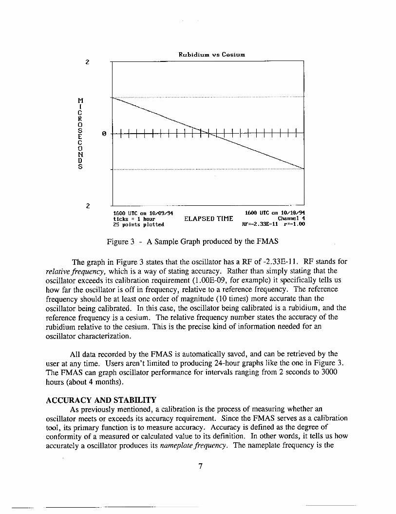
Figure 3 - A Sample Graph produced by the FMAS

The graph in Figure 3 states that the oscillator has a RF of -2.33E-11. RF stands for relative jirequcnq, which is a way of stating accuracy. Rather than simply stating that the oscillator exceeds its calibration requirement (1 .OOE-09, for example) it specifically tells us how far the oscillator is off in frequency, relative to a reference frequency. The reference frequency should be at least one order of magnitude (10 times) more accurate than the oscillator being calibrated. In this case, the oscillator being calibrated is a rubidium, and the reference frequency is a cesium. The relative frequency number states the accuracy of the rubidium relative to the cesium. This is the precise kind of information needed for an oscillator characterization.

All data recorded by the FMAS is automatically saved, and can be retrieved by the user at any time. Users aren’t limited to producing 24.hour graphs like the one in Figure 3. The FMAS can graph oscillator performance for intervals ranging from 2 seconds to 3000 hours (about 4 months).

ACCURACY AND STABILITY As previously mentioned, a calibration is the process of measuring whether an

oscillator meets or exceeds its accuracy requirement. Since the FMAS serves as a calibration tool, its primary function is to measure accuracy. Accuracy is defined as the degree of conformity of a measured or calculated value to its definition. In other words, it tells us how accurately a oscillator produces its namcpZate,frequency. The nameplate frequency is the

7

frequency labeled on the oscillator output. For example, an oscillator output labeled “5 MHz” is supposed to produce a ~-MHZ frequency. The relative frequency value tells us how close the actual frequency is to 5 MHz.

The FMAS uses relative frequency values to report accuracy. Relative frequency is dimen.sionZess, meaning that it does not refer to any particular averaging period, or any particular unit of measurement. For example, if we say that an oscillator has a relative frequency of l.OOE-09, it means that the oscillator’s frequency is off by 1 part in 109, or 1 part in 1 billion parts. This holds true if the nameplate frequency is 1 MHz, 5 MHz, 10 MHz, or something else. The relative frequency is independent of the nameplate frequency.

Even so, we can compute the actual frequency output of an oscillator if we know the nameplate frequency and the relative frequency. To illustrate this, Figure 3 is a graph of an oscillator with a nameplate frequency of 5 MHz that has a relative frequency of -2.33E-11. What is the actual output frequency of the oscillator? To find out, first multiply the nameplate frequency by the relative frequency:

(5 x 106) (-2.33 x IO-“) = -11.65 x IO-’ = -0.0001165 Hz

This is the frequency offset in Hz. The nameplate frequency is 5 MHz, or 5,000,OOO Hz. Therefore, the actual frequency is:

4,999,999.9998835 Hz

In addition to accuracy, the FMAS can also measure the stability of an oscillator. Stability is a description of the frequency change of an oscillator that occurs over time. A more proper term for these changes is probably instability, but the term stability is more widely used. Short-term stability usually refers to changes over intervals less than 100 seconds. Long-term stability can refer to measurement intervals greater than 100 seconds, but usually refers to periods longer than 1 day.

A statistical test used to measure stability is the Alhn Variance (AVAR), also called the two-sample or pair variance.6 AVAR graphs look different than the graphs used to measure accuracy. They don’t show the rate at which the oscillator is drifting, or how close the oscillator is to the correct frequency. Instead, they show the stability of the oscillator output with the drift removed. To illustrate this difference, Figures 4 and 5 both use data from the same 5-minute measurement period. Figure 4 shows the accuracy of the oscillator, and Figure 5 shows its stability.

8

-...

_...

_...

18 MHz Rubidium vs Cesium

1 I I I I I I I I I I I I I I I I I I I I I I I I Start line: 10-14-1994 (22:16:20) Duration: 300.08 seconds tick* = 10 seconds Channel 4 300 noints vlotted RF=-z.69E-ll r=-1.M)

Figure 4 : Acc&ac.y Plot of Rubidium over 5-Minute Period

18 MHz Rubidium vs Cesium -10

-11

-12

-13

I I

I I

0 1 2 3

LOG TAU <Seconds) N-14-1994 (22:16:28)

Figure 5 - Stability Plot (AVAR) of Rubidium over 5-Minute Period

9

AVAR plots use a logarithmic scale. The values along the x-axis (called tau values) represent the length of the averaging period in seconds. Each division represents an averaging period 10 times longer than the previous division. For example, a tau value of 2 represents an averaging period of 100 seconds (10’). A tau value of 3 represents an averaging period of 1000 seconds (10s).

The values along the y-axis represent the result of the measurement. A value of -10 means that the oscillator has a stability of 1 .OOE-10. This value should not be confused with the accuracy value (relative frequency). For example, an oscillator off in frequency by l.OOE-08 may reach a stability of l.OOE-12 in 1000 seconds. This means that even though the oscillator is producing a frequency off by 1 .OOE-08, it is doing so at a very stable rate.

A typical AVAR plot (like the one in Figure 5) shows the stability values improving as the measurement period increases in length. This will continue until the oscillator reaches its noisefloor, at which point the stability values will level out and then eventually start to get worse. Most oscillators reach their noise floor at a tau value of around 3. The FMAS is capable of measuring stability at a level of l.OOE-14 at a tau value of 3. This is good enough to measure nearly any oscillator.

SYSTEM SPECIFICATIONS

The table below lists the measurement specifications of the FMAS.

Number of Measurement Channels I 5

Input Frequencies Accepted by the System I 1, 5, and 10 MHz

Maximum Number of Data Points per

I

3000 Graph

Averaging Period (long term measurements)

1 hour

Averaging Period (short term measurements)

1 second

Single Shot Measurement Resolution I < 40 picoseconds

Accuracy using GPS (24 hours) I l.OOE-13

Stability (AVAR) after oscillator self-test of 1000 seconds

l.OOE-14

10

NIST SUPPORT NIST completely supports each customer of the NIST Frequency Measurement

Service. If any part of the FMAS fails, it is replaced immediately (usually overnight). Plus, each FMAS is shipped with remote communications software. This allows NIST to run each system from Boulder through the phone lines. NIST can diagnose and troubleshoot problems with the system, and view and graph the measurement data. If necessary, NIST can even perform maintenance on the computer, like optimizing the hard drive, recovering a damaged file, or installing an update to the measurement software.

NIST downloads the daily relative frequency values from each customer, and sends them a monthly report which certifies that their data is traceable. If the data is poor, NIST will investigate the problem (a poor GPS signal or bad oscillator, for example) and help the customer correct it. Technical support is provided by telephone Monday through Friday, during normal working hours.

LABORATORY ACCREDITATION One of the more valuable aspects of the NIST Frequency Measurement Service is that

it standardizes the way that a laboratory performs frequency calibrations. Customers no longer need to develop their own system for measuring frequency, or worry about whether their measurements are traceable. All customers record data in the same way, using the same measurement techniques developed by NIST. These techniques are well documented and widely accepted in the field of metrology.

Over the past few years, it has become increasingly important for calibration laboratories to become accredited, and for their companies to obtain ISO- registration. Some companies now view laboratory accreditation and ISO- registration as a prerequisite to doing business. The NIST Frequency Measurement Service can be a major asset to these laboratories since it conforms to the guidelines published by the National Voluntary Laboratory Accreditation Program (NVLAP), which became operational in May 1994. NVLAP is a NIST-operated program that assesses the technical competence of calibration labs, and grants accreditation to those who qualify.

The NVLAP guidelines are based on IS0 Guide 25, ISO-9002, and the ANSUNCSL 2540-l military standard. They are outlined in the NVLAP Calibration Laboratories Technical Guide (NIST Handbook l.5@2).7 This document includes technical descriptions of how calibrations should be made.

NVLAP can accredit laboratories in eight different areas of calibration (calledBeZds). Each field is divided into more detailed areas called parameters. For example, frequency calibration is a parameter in the time and frequency field. NIST Frequency Measurement Service customers can easily obtain NVLAP accreditation for frequency calibration if they choose to do so.

11

SUMMARY The NIST Frequency Measurement Service has been completely redesigned in 1994

and now offers many new benefits to the calibration laboratory. NIST has improved every aspect of the measurement system included with the service. These improvements include: a sub-nanosecond time interval counter, short-term stability measurements (AVAR), 1 .OOE- 13 accuracy in 24 hours using GPS, and full compliance with the NVLAP guidelines for frequency calibrations.

REFERENCES

George Kamas and Michael A. Lombardi, Time and Frequency User’s Manual, NIST Special Publication 559, 1990.

George Kamas and Michael A. Lombardi, “A New System for Measuring Frequency”, NCSL Conference Proceedings, 1985, pp. 224-23 1.

Michael A. Lombardi, “The Design Philosophy of the NIST Frequency Measurement Service”, NCSL Conference Proceedings, 1991, pp. 277-287.

Victor S. Zhang, Dick D. Davis, and Michael A. Lombardi, “High Resolution Time Interval Counter”, unpublished paper submitted to Precise Time and Time Interval Conference (PlTI), 1994.

Dennis Bodson, Robert T. Adair, and Michael D. Meister, “Time and Frequency Information in Telecommunication Systems Standardized by Federal Standard 1002A”, Proceedings of the IEEE, vol. 79, no. 7, pp. 1077-1079, July 1991.

D. B. Sullivan, D. W. Allan, D. A. Howe, and F. L. Walls, editors, Characterization of Clocks and Oscillators, NIST Technical Note 1337, 1990.

Jon M. Crickenberger, editor, NVLAP Calibration Laboratories Technical Guide, NIST Handbook 150-2, 1994.

12