the non-commutative geometry of penrose tilingsura-reports/043/mcmurdie.christopher/final.pdfpenrose...

The Non-Commutative Geometry of PenroseTilings

Christopher R. McMurdieAdvisors: Arlo Caine

Doug Pickrell

16 August 2004

Abstract

This paper represents work completed during the 2003-2004 academicyear, as well as summer 2004. It is written for a curious math undergrad-uate, assuming some limited background. Gelfand’s Theorem is provedin detail to provide familiarity with associating C*-algebras to compact,Hausdorff spaces. Penrose tilings are then studied, concluding with an al-gebraic characterization of the space of Penrose tilings using the methodsof algebraic K-theory.

This work was funded by the Mathematics Department at the Univer-sity of Arizona through an NSF VIGRE grant.

CONTENTS CONTENTS

Contents

1 Introduction 1

2 Compact Hausdorff Spaces 2

3 Abelian C*-Algebras 8

4 Penrose Tilings 13

5 Penrose Universe 15

6 Topological Approach 17

7 Algebraic Approach 19

8 K-Theory 20

9 Bibliography 23

1 INTRODUCTION

1 Introduction

This paper was written over the course of three semesters. The writing beganin the Fall of 2003, after working with Arlo Caine studying planar tilings. Duringthis time, we studied Penrose tilings in some depth. Many of these results arepresented in Section 4. By the end of the Fall semester, we decided to continuewith the full scope of the project, which required that I learn some more advancedmath. In the Spring of 2004, I proved the first part of Gelfand’s Theorem andthen in the beginning of the summer I completed the proof (Sections 2 and 3).At this point, I was ready to look at the advanced methods of non-commutativegeometry to study the non-commutative space of Penrose tilings. The results ofthis effort are presented in sections 5-8.

This paper is written for an undergraduate mathematics student with someknowledge of algebra and analysis. First, we will study Gelfand’s Theorem tosee how one can associate an abelian algebra with a space. The proof is given insufficient detail so that the intended audience, provided some standard referencesfor unfamiliar definitions, etc., can understand every step.

Once Gelfand’s theorem has been explained, we summarize the basic proper-ties of Penrose tilings. Then using these properties, we develop a way of codingPenrose tilings so that the set of all Penrose tilings can be analyzed. We brieflyattempt to use classical methods to study this space, but we find that thesemethods fail. Finally, we use methods from non-commutative geometry, and wesee that the results are successful.

I would like to thank Arlo Caine for the many hours he has spent teachingme. His ability to condense many large subjects and communicate them to ayoung undergraduate reveals his mastery. I would also like to thank Dr. DougPickrell for overseeing the project and assisting me when Arlo could not.

Sincerely,

Christopher McMurdie

1

2 COMPACT HAUSDORFF SPACES

2 Compact Hausdorff Spaces

Gelfand’s Theorem applied to compact Hausdorff spaces is the following state-ment:

X ∼= Spec C(X)

where X is a compact, Hausdorff space and C(X) denotes the abelian C∗−algebraof continuous, complex valued functions on the set, X. Gelfand’s theorem alsostates the converse, that every unital abelian C∗−algebra is isomorphic to contin-uous functions on some locally compact Hausdorff space. These two statementsshow that there is an equivalence of categories - studying some locally compactHausdorff space is like studying the associated abelian C∗−algebra.

We will prove the first part of Gelfand’s Theorem in this section, by showingthat there exists a bijective function from X onto Spec C(X). Then, we show thatthis relation is actually a homeomorphism between compact, Hausdorff spaces.First, we provide some background.

We begin by stating that C(X) is a complex vector space under pointwiseaddition. This is well known, and can easily be verified. Now, we show that it isa complex algebra under pointwise multiplication.

We know that an algebra is a vector space, which is equipped with an asso-ciative multiplication that commutes with scalars (from the field, over which thevectorsspace is defined). Here, we define

∀x ∈ X (f · g)(x) = f(x) · g(x)

and all of the conditions are clearly satisfied. It can also be pointed out that thisalgebra is abelian, since it inherits commutivity from multiplication on C.

We go further, and verify that C(X) is actually a C∗−algebra, by showingthat ∀f, g ∈ C(X),∀a ∈ C, ∃ ∗ : A→ A such that

(f ∗)∗ = f (f + g)∗ = f ∗ + g∗ (f · g)∗ = g∗ · f ∗ (a · f)∗ = a · f ∗

These identities are obvious when we recognize that each element of C(X) canbe decomposed: f(x) = f1(x) + i · f2(x), where f1, f2 are real valued. Then, the∗−operation is simply complex conjugation.

Finally, we verify that C(X) is a unital C∗−algebra, by showing that thereexists an element, f ∈ C(X) 3 ∀g ∈ C(X), ∀x ∈ X, (f · g)(x) = g(x). This isthe element f 3

∀x ∈ X f(x) = 1

2


Now that we have C(X) as a unital C∗−algebra, we would like to define anorm on C(X), such that C(X) is complete with respect to the metric inducedfrom the norm.

Define ‖ ‖: C(X)→ R such that

‖f ‖= maxx∈X|f(x)|

Clearly, this is a norm provided that the max exists. Since X is a compacttopological space, and ‖ f ‖ is a continuous function from X into R, we knowthat the function attains its maximum value.

We note that C(X) is complete with respect to this norm, though the proofis omitted.

Now, we’re ready to consider the relation between the set, X, and the set,Spec C(X). Spec C(X) is defined to be the set of all non-zero C∗−homomorphismsthat map elements of C(X) → C. We will now show that there is an injectivecorrespondence between points of these sets.

We will actually prove that every non-zero C∗−homomorphism, which we willcall φ, returns the value f(x) for some point x ∈ X. Then the injective relation-ship between X and the set of all φ’s is obvious: for every x, there is a φx suchthat ∀f ∈ C(X), φx(f) = f(x).

If φ : C(X) → C is a non-zero, C∗−homomorphism, then ∃x ∈ X 3 ∀ f ∈C(X), φx(f) = f(x).

Proof : We proceed by contradiction. Assume, then, ∀x ∈ X,∃f ∈ C(X) 3φx(f) 6= f(x). Since φ : C(X)→ C sends an infinite dimensional space to a onedimensional space, we know that the kernel of φ, the set {f ∈ C(X)|φ(f) = 0},is non-empty. Consider an x ∈ X. By our assumption, ∃fx 3 φ(fx) = 0 andfx(x) 6= 0. Since the kernel of a homomorphism is an ideal, we note that fx is inan ideal.

Now consider fx. Since φ is a C∗−homomorphism, it is clear that φ(fx) =φ(fx)

∗ = 0∗ = 0, so fx is also in this ideal. Now, since fx 6= 0, it must be thatfx 6= 0. Now, we have the non-zero product fx ·fx = |f |2, which is in ker(φ) (sinceit is an ideal). Now, we will use the compactness of X to show that 1 ∈ ker(φ).

For each x ∈ X, we have shown that we can find a continuous function |fx|2,that is real-valued and non-zero in some neighborhood about x. The union of allsuch neighborhoods is an open cover of the space, X. Then, since X is compact,we know that there exists a finite subcover, which covers X. Consider this finitesubcover. We have a finite set of functions, {fx1 , . . . , fxn}. Let f = |fx1|2 + . . . +|fxn|2. Since φ is linear, it must be that φ(f) = φ(|fx1 |2) + . . . + φ(|fxn|2) = 0, sof ∈ ker(φ), and f is continuous and non-zero over all of X.

3


Now, consider (f(x))−1. Since f is continuous and non-zero, so is (f(x))−1.Now, ker(φ) must contain the multiplicative identity, since f · (f(x))−1 must bein the ideal, by definition. This means that ker(φ) = C(X), since any idealcontaining the algebra’s identity must be the entire algebra. But this impliesthat φ is a zero homomorphism, contradicting our assumption. We conclude thatevery non-zero C∗−homomorphism must be evaluation at a point for some pointx ∈ X. �

At this stage in the proof, we have demonstrated a one-to-one correspondencebetween the compact Hausdorff space, X, and the set of all C∗−homomorphisms,Spec C(X). Now, we would like to demonstrate that there is a homeomorphismbetween these compact Hausdorff spaces. Of course, this requires that we imposea canonical Hausdorff topology on Spec C(X).

We notice that Spec C(X) is actually a subset of a much larger space, C(X)∨.This is called the dual space of C(X), and is defined as the set of all continuous,linear functionals mapping the algebra to its base field (in this case C). Clearly,this differs from Spec C(X), since it lacks the strict requirement that these func-tionals be multiplicative homomorphisms. There is a natural topology to put onthis larger space, called the weak−∗ topology. This topology is generated by setsof the form:

N(φ0 : S, ε) := {φ ∈ C(X)∨ : |φ(f)− φ0(f)| < ε ∀f ∈ S ⊂ C(X)}

where S must be a finite subset. We note explicitly that each basis element de-pends on three parameters: φ0, ε, S. We would like to show that the following:

The weak−∗ topology is Hausdorff.

Proof : To show that this topology is Hausdorff, we consider φ1, φ2 ∈ C(X)∨ 3φ1 6= φ2. We want to show that there are two neighborhoods containing φ1, φ2, re-spectively, that are disjoint. We proceed constructively, by finding neighborhoodswhich meet these requirements.

First, we define the parameters. Let N1 = N(φ1 : {g}, ε), and let N2 = N(φ2 :{g}, ε) for any g 3 φ1(g) 6= φ2(g) (Such a g must exist since φ1 6= φ2). Then, let

ε = |φ1(g)−φ2(g)|2

.Thus, we have the following neighborhoods:

N1 = {φ ∈ C(X)∨ : |φ(g)− φ1(g)| < |φ1(g)− φ2(g)|2

}

N2 = {φ ∈ C(X)∨ : |φ(g)− φ2(g)| < |φ1(g)− φ2(g)|2

}

By our choice of g, it is clear that both neighborhoods are non-empty, forthey must contain φ1, φ2 respectively. Furthermore, these neighborhoods have

4


null intersection. �

Now, we would like to define a norm on C(X)∨. Consider any φ ∈ C(X)∨. It

can be verified that there is a bound on |φ(f)|‖f‖ that is independent of f ∈ C(X).

Then, we define ‖ ‖: C(X)∨ → R as

‖φ‖= supf 6=0

|φ(f)|‖ f ‖

‖ ‖ defines a norm on C(X)∨.

Proof : We verify that this definition satisfies the conditions. |φ(f)|‖f‖ > 0 ∀f 6=

0 ∈ C(X) by definition of absolute value and the norm. It follows that thissupremum must also be positive. Now, consider α ∈ C. Then, clearly ‖α · φ ‖=|α|· ‖ φ ‖, by properties of φ and suprema. Finally, since suprema respect thetriangle inequality, we have that ∀φ1, φ2 ∈ C(X),

‖φ1 + φ2 ‖≤‖φ1 ‖ + ‖φ2 ‖. �

In order to prove that Spec C(X) is a compact Hausdorff space, we will needto show that it is a closed subset of the unit ball, which is compact in the weak-∗

topology by the Banach-Alaoglu Theorem.

Spec C(X) is bounded by the unit ball in C(X)∨.

Proof : We consider an arbitrary φx ∈ Spec C(X). Then φ is given by evalu-ation at x. We want to show that the norm of φ is ≤ 1.

Now, ‖ φx ‖= supf 6=0|φx(f)|‖f‖ , and we defined ‖f ‖= maxx∈X |f(x)|. Combining

these expressions, we have that

‖φx ‖= supf 6=0

|φx(f)|maxx∈X |f(x)|

Clearly, ‖ φx ‖≤ 1 iff |φx(f)|maxx∈X |f(x)| ≤ 1∀f ∈ C(X). But this result is obvious,

because |φx(f)| = |f(x)| ≤ maxx∈X |f(x)| by definition of maximum. Notice thatwe can easily verify that ∀x ∈ X, ‖φx‖ = 1. We only need to check that thereexists an f ∈ C(X) that attains its maximum value at x, since this would lead

to maxx∈X |f(x)|maxx∈X |f(x)| = 1. Clearly, the unital (f(x) = 1,∀x) satisfies this property. �

Spec C(X) is closed in the weak∗−topology.

Proof: To show that Spec C(X) is closed, we must show that its complement isopen in the weak∗−topology. Thus, we want to construct an open set containing

5


C(X)∨\Spec C(X). Clearly, this can be done if we can find an open set aroundan arbitrary point in C(X)∨\Spec C(X) that is disjoint from Spec C(X).

We consider an element, φ ∈ C(X)∨\Spec C(X), where φ 6= 0. Since φ ∈C(X)∨, φ is a continuous, linear functional from C(X) → C. In particular, φ isnot in Spec C(X), which means that it cannot be multiplicative. So, there mustexist some elements, f, g ∈ C(X) 3 φ(f) ·φ(g) 6= φ(fg). Also, since the elementsof C(X)∨ are continuous and linear, they must be bounded. Thus, there existssome k ∈ R 3 ∀w ∈ C(X)∨,∀ f ∈ C(X), |w(f)| ≤ k‖f‖.

Consider the neighborhood N(φ : {f, g, f · g}, |φ(f ·g)−φ(f)·φ(g)|1+k(‖f‖+‖g‖) ). One can show

that this neighborhood contains φ and no element of Spec C(X). �

Because Spec C(X) is bounded by the unit ball, and is closed, Spec C(X)is compact by the Banach-Alaoglu Theorem. Thus, we have established thatSpec C(X) is a compact, Hausdorff space. Now, we want to find a homeomor-pishm between X and Spec C(X) to complete this part of Gelfand’s Theorem.

Define Φ : Spec C(X)→ X by Φ(φx) = x. We will show that this is a contin-uous bijection between compact, Hausdorff spaces. We will then show that sucha function is a homeomorphism. First, we must verify the following:

Φ is continuous.

Proof : To show that Φ is continuous, we will show that the pre-image of anyclosed set in X is closed in Spec C(X). So, we consider a closed set, C ∈ X. Wewill show that Φ−1(C) is closed, by showing that its complement inside Spec C(X)is open. So, specifically we want {φx ∈ Spec C(X)|Φ(φx) 6∈ C} to be an openset. This corresponds to the set{y ∈ X|y 6∈ C}. From Uryshon’s lemma, define afunction fy : X → R such that fy(y) = 0 and fy(z) = 1, ∀z ∈ C. So we considera neighborhood

N(φy : fy,1

2) = {w ∈ Spec C(X) : |w(fy)− φy(fy) <

1

2}

Then, using our definition of fy,

N(φy : fy,1

2) = {w ∈ Spec C(X) : |w(fy)| <

1

2}

So we have shown that the complement of Φ−1(C) is closed. It follows that Φ iscontinuous. �

Φ is a Homeomorphism between compact Hausdorff spaces.

Proof : To prove this result, we must show that Φ is bijective, continous, andthat Φ−1 is continuous. Since we have already shown that the first two conditionsare satisfied, it remains to show that Φ−1 is continuous.

6


Consider a closed subset A ⊆ Spec C(X). Then, A is compact since it is aclosed subset of a compact space. Φ(A) must be compact because it is the imageof a compact space under a continuous map. Finally, Φ(A) is closed in X sinceevery compact subspace of a Hausdorff space is closed.

So we have established that every closed subset in the domain space is closedin the image space. This verifies that Φ−1 is continuous. It immediately followsthat Φ is a homeomorphism between compact, Hausdorff spaces. �

This proves that X ∼= Spec C(X), and completes Part I.

7

3 ABELIAN C*-ALGEBRAS

3 Abelian C*-Algebras

The second half of Gelfand’s Theorem says:

A ∼= C(SpecA)

where, A is any abelian unital C∗−algebra.

Now, we should recall the spectrum of an element of a C∗−algebra; If A×

denotes the set of invertible elements of A, then the spectrum of some x ∈ A is

σ(x) := {λ ∈ C|λ · 1A − x 6∈ A×}

We can say that the spectrum of an element is the complement of the resolventset. Remember, the spectrum of the algebra is not the collection of σ(x) for allx ∈ A, but is the set of non-zero ∗−homomorphisms from A→ C.

This part of Gelfand’s Theorem says that every abelian C∗− algebra looks likethe algebra of continuous, complex valued functions on some compact Hausdorffspace. To prove this result, we will show the existence of a bijective function fromA onto C(SpecA) called the Gelfand Transform, which preserves complex conju-gation and all algebraic structure. This demonstrates that the Gelfand Transformis the required ∗−isomorphism.

The Gelfand Transform

ˆ: A→ C(SpecA) ∀x ∈ A, x 7→ x x : SpecA→ C ∀` ∈ SpecA, x(`) := `(x)

We would like that ˆ be a bijective homomorphism, as this would establish theisomorphism. First, we will prove thatˆis injective. To do this, we will show thatˆis an isometry. We begin by showing that

For every x ∈ A, range(x) = σ(x)

Proof : Fix x ∈ A. Consider y ∈ Ran(x). Then, ∃ ` ∈ SpecA 3 `(x) = y. Wewant to show that `(x) ∈ σ(x). This means that we want `(x) · 1A− x 6∈ A×. Weproceed by contradiction.

Suppose `(x) · 1A − x ∈ A×. This means ∃ a ∈ A 3 a = (`(x) · 1A − x)−1. Werewrite this as

a =1A

`(x) · 1A − x=

1

`(x)· 1A

1A − x`(x)

=1

`(x)·∞∑

k=0

(x

`(x)

)k

Note that this representation in A is unique since the inverse of an element of aC∗−algebra is unique. However, this some can only converge in A if ‖ x

`(x)‖< 1.

8


This means, that 1|`(x)| ‖x ‖< 1 and so ‖x ‖< |`(x)|. But, this contradicts what

we know about C∗−homomorphisms, namely that they are contractive (whichmeans, ∀x ∈ A, |`(x)| ≤ ‖x‖). Therefore, a does not exist, and so `(x) · 1A − x 6∈A×. This proves that Ran(x) ⊆ σ(x).

Now we prove the reverse inclusion. Consider λ ∈ σ(x). We want to showthat there exists an ` ∈ SpecA such that `(x) = λ. By definition of the spectrum,we see that λ · 1A − x is not invertible. Notice that this element generates anideal, I, of A:

I = {a · (λ · 1A − x)|a ∈ A}

This cannot be all of A becasue it cannot contain the element 1A. Thus, using theAxiom of Choice we can find some maximal ideal which contains I. Every max-imal ideal is the kernel of some ` ∈ SpecA, so for this `, `(λ · 1A − x) = 0. Then,since ` is a homomorphism, `(λ ·1A−x) = λ ·`(1A)−`(x) = 0⇒ λ = `(x) = x(`).So, λ ∈ Ran(x), and it follows that Ran(x) = σ(x). �

We now would like to show that ˆ is a homomorphism of C−algebras. Ahomomorphism preserves algebraic structure, so we would like to show that∀x, y ∈ A,∀λ ∈ C

x · y = x · yλ · x + y = λx + y

Since these functions share the same domain (SpecA), we proceed by consideringthe action on ` ∈ SpecA. x · y(`) = `(x · y) = `(x) · `(y), since ` is multiplicative.Also, `(x) · `(y) := x(`) · y(`). Thus, for all ` in the domain, x · y = x · y.

Similarly,înherits linearity from that of ` ∈ SpecA. Soîs a homomorphism.

We will show that ˆ is a bounded operator. Since it is linear, this will alsoimply thatîs continuous.

‖x‖∞ ≤ ‖x‖, ∀x ∈ A

Proof : Fix x ∈ A. Then, ‖x‖∞ := max`∈SpecA |x(`)| = max`∈SpecA |`(x)| ≤‖x‖, since ∀` ∈ SpecA, |`(x)| ≤ ‖x‖ (` is contractive). So, ‖x‖∞ ≤ ‖x‖. �

Let us prove thatîs a ∗−homomorphism. This means, we want to show that∀x ∈ A, x = x∗. However, we first define what is meant by x. For ` ∈ SpecA, letx(`) = x(`).

Proof : Fix x ∈ A. Consider ` ∈ SpecA. x∗(`) = `(x∗) = `(x)∗, since ` is a∗−homomorphism. This means, x∗(`) = x(`) = x(`), by definition. �

9


Definition: We define the spectral radius of x ∈ A as

r(x) := supλ∈σ(x)

|λ|

It is a theorem of Kato that limn→∞ ‖xn‖ 1n always exists and is equal to r(x).

If x is self-adjoint, then r(x) = ‖x‖.

Proof : We will establish that r(x) = ‖x‖ by showing that limn→∞ ‖xn‖ 1n =

‖x‖. Since ∀n ∈ N, ∃m ∈ N 3 2m > n, it suffices to show that ∀m ∈N, ‖x2m‖ 1

2m = ‖x‖. We proceed by induction.

Let m = 1. Starting from the left, we have ‖x2‖ 12 = ‖x∗x‖ 1

2 since x = x∗ (x

is self-adjoint). Then, by the C∗−identity, ‖x∗x‖ 12 = (‖x‖2)

12 = ‖x‖.

Now, let m = k + 1. Starting from the left, we have

‖x2k+1‖1

2k+1 = ‖(x2k

)2‖1

2k+1 = ‖(x∗x)2k‖1

2k+1 = ‖(x)2k

(x)2k‖1

2k+1

Then, using that x = x∗ and the C∗−identity we have

‖(x∗)2k

(x)2k‖1

2k+1 = (‖x2k‖2)1

2k+1 = ‖x2k‖1

2k = ‖x‖

by the induction hypothesis, which completes the proof. �

If x is self-adjoint, ‖x‖∞ = ‖x‖.

Proof : Fix x ∈ A. ‖x‖∞ := max`∈SpecA |x(`)|. This means that ‖x‖∞ :=maxy∈Ran(x) |y| = maxy∈σ(x) |y|, since Ran(x) = σ(x). Now, recognize that SpecAis compact, and so its image is compact in C. Then, by Heine-Borel, its im-age is closed and bounded in C. In particular, this means that maxy∈σ(x) |y| =supy∈σ(x) |y| = r(x) = ‖x‖, since x is self-adjoint. �

Now, we will prove thatˆis an isometry, meaning ∀x ∈ A, ‖x‖∞ = ‖x‖. Thiswill immediately lead to the injectivity of ˆ.

ˆ is an isometry.

Proof : Fix x ∈ A. Then, ‖x∗x‖∞ = ‖x∗x‖, since x∗x is self-adjoint. Now,‖x∗x‖ = ‖x‖2 by the C∗−identity. So we have that ‖x∗x‖∞ = ‖x‖2. This meansthat sup`∈SpecA |`(x∗x)| = ‖x‖2. But,

sup`∈SpecA

|`(x∗x)| = sup`∈SpecA

|`(x∗)`(x)| = sup`∈SpecA

|`(x)∗`(x)|

10


which again by the C∗−identity (now on C) gives

sup`∈SpecA

|`(x)|2 = ‖x‖2 ⇔ sup`∈SpecA

|`(x)| = ‖x‖

This means that ‖x‖∞ = ‖x‖. �

ˆ: A→ C(SpecA) is injective

Proof : Consider x, y ∈ C(SpecA) 3 x = y. We will prove that x = y.x = y ⇒ x − y = 0 ⇒ x− y = 0, sinceˆis linear. Then, ‖x− y‖∞ = ‖x − y‖ =0⇒ x− y = 0. So x = y. �

It remains only to show thatˆ: A → C(SpecA) is surjective. To do this, wewill employ the Stone-Weierstrass theorem.

Stone-Weierstrass Theorem: Let Z be a compact Hausdorff space, andlet B be a closed ∗−subalgebra of continuous functions on Z, which separatespoints of Z and contains the constant function. Then B = C(Z).

Now, we will try to prove that A := {x|x ∈ A}, which is the range of , theGelfand transform, satisfies the conditions of B above; SpecA will function as Z,the compact Hausdorff space. If we can show that the hypotheses of this theoremare satisfied, then we will have shown that the range ofˆ is equal to C(Spec A),verifying thatˆis surjective. We now verify the hypothesis that A seperates thepoints of Spec A.

A separates the points of Spec A.

Proof : We wish to verify that ∀`1, `2 ∈ SpecA,∃x ∈ A such that `1 6= `2 ⇒x(`1) 6= x(`2). We proceed by contradiction.

Assume that ∃`1, `2 ∈ SpecA 3 `1 6= `2 and ∀x ∈ A, x(`1) = x(`2). Thismeans that ∀x ∈ A, `1(x) = `2(x). This, of course, means that these functionalsare equal, since they have the same domain and are equal over this space, con-tradicting that `1 6= `2. This proves that A separates the points of SpecA. �

It remains only to verify that A is closed, for then all of the hypotheses aresatisfied.

A is closed.

Proof : We want to show that A is closed by showing that it contains allof its limit points. Thus, we consider an arbitrary limit point x. For A to beclosed, we must show that x ∈ A. Now, since x is a limit point, there is some net

11


(xα)α∈J → x. Then, sinceˆis injective, we can construct an equivalent net in thedomain, X. We must show that this net, (xα)α∈J → x ∈ A. Sinceˆis an isome-try, we know that it preserves distances. In particular, if a net converges in oneset, it must converge in the other. Thus, (xα)α∈J → x ∈ A, so then A is closed. �

We have shown that A = C(Spec A), which proves that ˆ : A → C(Spec A)is surjective. Thus, ˆ is a ∗−homomorphic bijection, and establishes that A isisomorphic to C(Spec A).

12

4 PENROSE TILINGS

4 Penrose Tilings

We will begin our discussion of Penrose Tilings by introducing what we meanby a tiling of the plane. We will define a two-dimensional tiling, or tesselation,as a partitioning of the plane into a finite set of prototiles. Each prototile is afinite subset of the plane which is homeomorphic to the unit sphere.

A familiar example of a tiling might be a grid of squares. In this case there isonly one prototile. Another property of this simple tiling is translational symme-try. We say that a tiling exhibits translational symmetry if there exists a non-zerovector of translation which maps the tiling identically to itself.

If a tiling does not have vectors of translational symmetry, we say that thetiling is aperiodic. Penrose tilings are perhaps the simplest aperiodic tilings,because they consist of only two prototiles. The prototiles are each isosceles tri-angles, one with acute and one with obtuse vertex angles, respectively. There isa matching condition as indicated in the figures below.

Notice that there are only two different edge lengths in the figure. If we con-sider the shorter length in the diagram to be the unit, then we find that the otherlength is τ = 1+

√5

2, the Golden ratio.

Here is an example of a penrose tiling with acute and obtuse prototiles coloredblue and red, respectively.

13

4 PENROSE TILINGS

Constructing a Penrose tiling can be an interesting excercise to do by hand.However, the only way to ensure that any Penrose tiling of the entire plane evenexists is to define a decomposition. We begin with some collection of prototiles,and we define an algorithm that partitions these prototiles into new prototilesthat are geometrically similar, but reduced in size by some scale factor. This de-composition could be followed by magnification by the scale factor. This process,if it exists, could be repeatedly arbitrarily. We will now define this process forPenrose tilings, proving that arbitrarily large Penrose tilings exist.

1

3

5

2

4

→∞

We summarize the decomposition illustrated above by noting that after twodecomposition steps the acute triangle is decomposed into two acute trianglesand an obtuse, while the obtuse triangle is decomposed into an obtuse and anacute. Symbolically, we can write

An+1 = 2An + On On+1 = An + On

14

5 PENROSE UNIVERSE

where Ai (resp. Oi) is the number of acute (obtuse) prototiles after 2i decom-positions. Also, note that after each step (instead of every two steps) the size ofthe respective prototiles changes. At stage 2, we see that the obtuse prototile isnow larger than the acute. Indeed, at every stage of decomposition, the ratio ofthe area of the prototiles is τ , however the larger prototile alternates between theacute and the obtuse. This observation is important, and for this reason we willcall the larger prototile in a Penrose tiling Big, and the smaller prototile Small.

We note that the altitudes and base of the acute prototile also have the ratioτ : 1 and the obtuse prototile has the ratio 1 : τ . This fact can be proven withelementary geometric methods, and so is ommitted. Now, we will determine howmuch of the tiling is made from acute prototiles and how much is from obtuse.Let λn be the ratio of the number of acute prototiles to the number of obtuse,after n decompositions. Then,

λn+1 =An+1

On+1

=2An

On+ 1

An

On+ 1

=2λn + 1

λn + 1

The limit as n → ∞ is τ . Since the ratio of areas of the prototiles is τ , theamount of the plane in the acute partition to the obtuse partition must oscillatebetween τ 2 : 1 and 1 : 1.

We now have enough information to prove that Penrose tilings are aperiodic.Consider any (infinite) periodic tiling, T , of the plane. Since T is periodic, thereexists a finite patch of T (which itself is homeomorphic to the unit ball) suchthat T is covered by a disjoint union of copies of this finite patch. The ratio ofprototiles in the infinite tiling must be exactly equal to the ratio of the prototileswhich form the patch. Since this patch is finite, the ratio is necessarily rational.It follows that any tiling of the plane that has an irrational ratio of prototiles cannot be periodic.

5 Penrose Universe

In this section we will discuss the set of all Penrose tilings, called the PenroseUniverse. Up until this point, we have not ruled out the possibility that thereis only one Penrose tiling. To investigate this, we will need to develop a systemthat can describe a Penrose tiling. First we will have to explore a process calledcomposition.

Composition is essentially the inverse process of decomposition. Instead ofseparating larger prototiles into smaller ones, we will erase lines to create a tiling

15

5 PENROSE UNIVERSE

with larger prototiles. At each stage, we erase only the lines that would be in-troduced using the reverse process of composition.

We can describe a Penrose tiling by beginning with some prototile in thetiling, and then composing the tiling one stage. After each composition we noteif the new prototile functions as a Big or a Small (B or S) in the current tiling.

1

3

5

2

4

6

We can see in the particular example above, the starting prototile begins asa Big (B). The sequence describing this tiling is then B-S-B-S-B-B.

Complete Penrose tilings can be described in terms of these infinite binarysequences. There is a restriction, however, from all binary sequences, because wenotice that in no tiling can a Short prototile be composed into a Short prototile.Therefore, there is a grammar rule in the sequence, where an S is always followedby a B.

Further, we recognize that the choice of initial prototile is arbitrary. For thisreason, we must say that two tilings are equivalent if and only if the infinite tailsof their binary sequences are equivalent after some finite number of digits in thesequence. We will denote this equivalence relation as ∼.

Now, any Penrose tiling can be constructed directly from a sequence satisfyingthe grammar rules. Thus, if we can produce two sequences which satisfy thegrammar rules and do not ever agree, then we will have shown the existenceof more than one Penrose tiling. The alternating sequence BSBSBS... and the

16

6 TOPOLOGICAL APPROACH

sequence BBSBBS... are such examples. In fact, it is easy to see now that thereare an uncountably infinite number of unique Penrose tilings.

6 Topological Approach

We want to induce a metric on this space of Penrose Tilings. Let X denote thespace of infinite binary sequences that satisfy the grammar rule. For this purpose,let B be represented by 1, and S be represented by 0. For y, z ∈ X, let

d(y, z) =∞∑

n=1

2−n|yn − zn|

where yi and zi are the ith digits in the y, z binary sequence, respectively. Weassert that d : X → R is a metric, though we only verify the triangle inequality.

∀x, y, z ∈ X, d(x, y) + d(y, z) ≥ d(x, z).Proof : Consider x, y, z ∈ X. We want to show that

∞∑n=1

2−n|xn − yn|+∞∑

n=1

2−n|yn − zn| ≥∞∑

n=1

2−n|xn − zn|

Now, using the triangle inequality on R, we know that for all n of the summation,|xn − yn| + |yn − zn| ≥ |xn − zn|. Our result follows immediately. Similarly, theother two conditions we did not verify are inherited directly from the absolutevalue metric on R. �

We will now investigate this metric space, (X, d). Remember that we havethis space partitioned into equivalence classes based on the equivalence relationstated earlier: if two binary sequences agree completely after some finite numberof digits, then they are equivalent.

Consider two distinct Penrose tilings, represented by their sequences x, y ∈ X.Since x, y are distinct, we know that d(x, y) = r for some positive r ∈ R. We canconstruct another sequence, x1, that is equivalent to x and such that d(x, y) < r.The construction is the following: find the first digit n where |xn − yn| 6= 0.Since x and y satisfy the grammar rule, this will not be a digit that is forced(i.e. it will not be a 1 following a 0). Thus, we can let xn = yn. Clearly,d(x1, y) = r − 2−n < r. However, we need not stop with x1. Repeating thisprocess arbitrarily, we can see that there exists a Penrose tiling, represented byxk, which can be made arbitrarily “close to” y under the metric d.

We conclude that every equivalence class is dense in X, since every sequencein X can be made arbitrarily close to a sequence in a given class. This means

17

6 TOPOLOGICAL APPROACH

that if we look at the space X/ ∼, the set of equivalence classes, we see that itis topologically very strange: the closure of any element in X/ ∼ is the wholespace.

Suppose that we try and construct an abelian algebra related to this space,to try and understand the set algebraically. This algebra, A, would be {f ∈C(X) 3 f(x) = f(y) ⇔ x ∼ y}. However, this would imply that A ∼= C,since a continuous function taking the same value on a dense set is constant. Sothis picture suggests that X is a one-point space; however, we know this set isuncountable.

Thus, neither the topology induced from the metric, nor the abelian algebraassociated to the space reveals anything about the structure of the Penrose uni-verse. We will see in the next section that associating a non-abelian algebra tothis space is the appropriate method for further study.

18

7 ALGEBRAIC APPROACH

7 Algebraic Approach

In this section, we will associate a non-commutative C∗−algebra to the space ofPenrose tilings. Then, we will use the methods of algebraic K-theory to classifythe associated algebra.

The set of binary sequences that obey the grammar rule, X, has two struc-tures: a metric which gives rise to a topology and an equivalence relation, whichpartitions the set. We have shown that these structures are not intuitively “con-sistent,” and in general it can be difficult to associate an algebra to such a space.However, we can show that X/ ∼ is a projective limit of finite spaces, giventhe decomposition algorithm outlined in section 4. So we will exploit a standardmethod for associating a matrix algebra with a finite set and equivalence relation.

Now, we will explain what we mean by the projective limit of finite spaces.

(X1,∼1)←− (X2,∼2)←− (X3,∼3)←− · · · (1)

Each Xi is the set of all finite binary sequences that satsify the grammer rule,and contain i digits, and each ∼i is the equivalence relation where the sequencesare exactly equivalent after i digits. The projection from (Xi+1,∼i+1) −→ (Xi,∼i

) is the obvious projection: delete the last digit in each sequence of Xi+1. Wealso note that each space has only two equivalence classes, since the last digit ofany sequence in Xi is either a B or an S, which partitions the set.

At each stage we will have two partitions, each corresponding to the lastdigit of the sequence being 0 or 1. Suppose we are given a finite set, Xn ={x1, . . . xi, xi+1, xn} with 2 equivalence classes, and such that xj ∈ Partition 1 forj ≤ i, and else xj ∈Partition 2. The, the associated matrix algebra is

C∗(Xn,∼) =

a11 . . . a1i 0 . . . 0...

. . ....

.... . .

...ai1 . . . aii 0 . . . 00 . . . 0 a(i+1)(i+1) . . . a(i+1)n...

. . ....

.... . .

...0 . . . 0 an(i+1) . . . ann

|aij ∈ C

Clearly, this matrix algebra is the direct sum of two other matrix algebras,

the rank of each being equal to the number of elements in that partition. Herewe find that the rank of these sub-algebras will be the Fibonacci numbers: eachsequence in Xi that ends in S must be followed by a B in Xi+1 because of thegrammer rule; however, each series in Xi ending in B can be followed by a B or S.Indeed, since each finite space contains all possible sequences, we can determine

19

8 K-THEORY

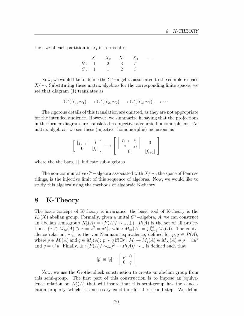
the size of each partition in Xi in terms of i:

X1 X2 X3 X4 · · ·B : 1 2 3 5S : 1 1 2 3

Now, we would like to define the C∗−algebra associated to the complete spaceX/ ∼. Substituting these matrix algebras for the corresponding finite spaces, wesee that diagram (1) translates as

C∗(X1,∼1) −→ C∗(X2,∼2) −→ C∗(X3,∼3) −→ · · ·

The rigorous details of this translation are omitted, as they are not appropriatefor the intended audience. However, we summarize in saying that the projectionsin the former diagram are translated as injective algebraic homomorphisms. Asmatrix algebras, we see these (injective, homomorphic) inclusions as

[|fi+1| 0

0 |fi|

]−→

∣∣∣∣ fi+1 ∗∗ fi

∣∣∣∣ 0

0 |fi+1|

where the the bars, | |, indicate sub-algebras.

The non-commutative C∗−algebra associated with X/ ∼, the space of Penrosetilings, is the injective limit of this sequence of algebras. Now, we would like tostudy this algebra using the methods of algebraic K-theory.

8 K-Theory

The basic concept of K-theory is invariance; the basic tool of K-theory is theK0(X) abelian group. Formally, given a unital C∗−algebra, A, we can constructan abelian semi-group K ′

0(A) = (P (A)/ ∼vn,⊕). P (A) is the set of all projec-tions, {x ∈ M∞(A) 3 x = x2 = x∗}, while M∞(A) =

⋃∞n=1 Mn(A). The equiv-

alence relation, ∼vn is the von-Neumann equivalence, defined for p, q ∈ P (A),where p ∈Mi(A) and q ∈Mj(A): p ∼ q iff ∃r : Mi →Mj(A) ∈M∞(A) 3 p = uu∗

and q = u∗u. Finally, ⊕ : (P (A)/ ∼vn)2 → P (A)/ ∼vn is defined such that

[p]⊕ [q] =

[p 00 q

]Now, we use the Grothendieck construction to create an abelian group from

this semi-group. The first part of this construction is to impose an equiva-lence relation on K ′

0(A) that will insure that this semi-group has the cancel-lation property, which is a necessary condition for the second step. We define

20

8 K-THEORY

a new abelian semi-group, K+0 (A) = K ′

0(A)/ ∼c. For p, q ∈ K ′0(A), p ∼c q iff

∃r ∈ K ′0(A) 3 p⊕ r = q ⊕ r.

Now, we will construct an abelian group, K0(A) from K+0 (A). This second

part of the Grothendieck construction is defined by K0(A) = K+0 (A)2/ ∼g, where

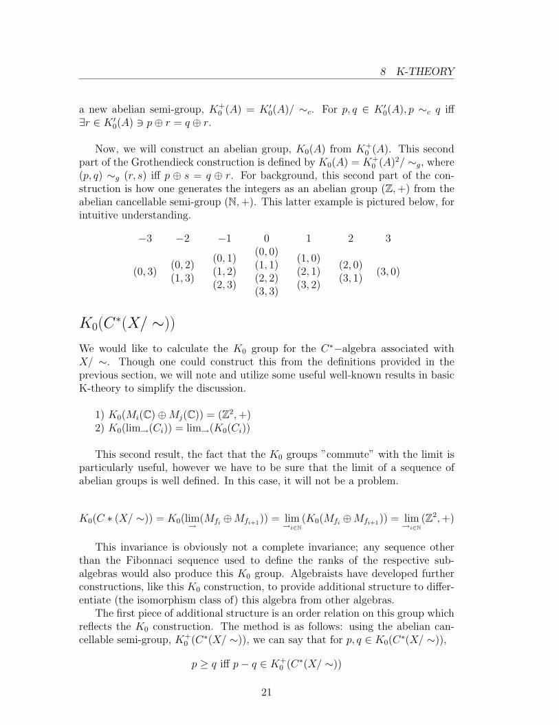
(p, q) ∼g (r, s) iff p ⊕ s = q ⊕ r. For background, this second part of the con-struction is how one generates the integers as an abelian group (Z, +) from theabelian cancellable semi-group (N, +). This latter example is pictured below, forintuitive understanding.

−3 −2 −1 0 1 2 3

(0, 3)(0, 2)(1, 3)

(0, 1)(1, 2)(2, 3)

(0, 0)(1, 1)(2, 2)(3, 3)

(1, 0)(2, 1)(3, 2)

(2, 0)(3, 1)

(3, 0)

K0(C∗(X/ ∼))

We would like to calculate the K0 group for the C∗−algebra associated withX/ ∼. Though one could construct this from the definitions provided in theprevious section, we will note and utilize some useful well-known results in basicK-theory to simplify the discussion.

1) K0(Mi(C)⊕Mj(C)) = (Z2, +)2) K0(lim→(Ci)) = lim→(K0(Ci))

This second result, the fact that the K0 groups ”commute” with the limit isparticularly useful, however we have to be sure that the limit of a sequence ofabelian groups is well defined. In this case, it will not be a problem.

K0(C ∗ (X/ ∼)) = K0(lim→(Mfi

⊕Mfi+1)) = lim

→i∈N(K0(Mfi

⊕Mfi+1)) = lim

→i∈N(Z2, +)

This invariance is obviously not a complete invariance; any sequence otherthan the Fibonnaci sequence used to define the ranks of the respective sub-algebras would also produce this K0 group. Algebraists have developed furtherconstructions, like this K0 construction, to provide additional structure to differ-entiate (the isomorphism class of) this algebra from other algebras.

The first piece of additional structure is an order relation on this group whichreflects the K0 construction. The method is as follows: using the abelian can-cellable semi-group, K+

0 (C∗(X/ ∼)), we can say that for p, q ∈ K0(C∗(X/ ∼)),

p ≥ q iff p− q ∈ K+0 (C∗(X/ ∼))

21

8 K-THEORY

It will be useful to explicitly determine what this ‘positive’ subset, K+0 ⊂ K0 =

Z2, actually contains.

We see that the transition matrix associated to consecutive algebras, i.e.

C∗(Xi/ ∼i), C∗(Xi+1,∼i+1), is

[1 11 0

]. Thus, we want to know the points

of Z2 which will be ‘positive,’ i.e. end up in N2 after a finite applications of thetransition matrix. The standard method calls for the eigenvalues and eigenvec-tors of the transition matrix to help determine a phase portrait. We find that

λ1 = τ

λ2 =−1

τ

v1 =

[τ1

]

v2 =

[1−τ

]It follows that K0(C

∗(X/ ∼) = {(x, y) ∈ Z2 3 τx + y ≥ 0} )

Unfortunately, this ordered group, (K0(C∗(X/ ∼)), K+

0 (C∗(X/ ∼))), calledthe dimension group, is still not a complete invariant. To produce the completeinvariant, another set, called the scale is introduced and associated with the al-gebra. One definition of the scale is Γ(A) = {p ∈ K+

0 (C ∗ (X/ ∼)) 3 p ≤ 1A}. Inthis case, we find that the scale is Γ = {(x, y) ∈ Z2|0 ≤ τx + y ≤ τ + 1}. Withthis final algebraic characteristic, we have the complete invariant of C∗(X/ ∼),the algebra associated with the space of all Penrose tilings.

We notice the multiple appearance of τ in this algebraic invariant. Given τ ’smultiple roles in the construction of Penrose tilings, we see that the study of thisnon-commutative algebra gave insight into the structure of the space of Penrosetilings.

22

9 BIBLIOGRAPHY

9 Bibliography

This paper followed closely the following pre-print:

Tasnadi, Tamas. Penrose Tilings, Chaotic Dynamical Systems andAlgebraic K-Theory. 10 Apr 2002. http://arxiv.org/abs/math-ph/0204022

The following reference is the standard for studying tesselations:

B. Grunbaum and G.C. Shephard. Tilings and Patterns. Freeman,New York, 1989.

These volumes are useful in understanding the details of Algebraic K-Theory:

A.J. Berrick and M.E. Keating. An Introduction to Rings and Mod-ules with K-theory in View. Cambridge, 2000.

M. Rørdam, F. Larsen and N. Laustsen. An Introduction to K-Theoryfor C∗−algebras. Cambridge, 2000.

23

the non-commutative geometry of penrose tilingsura-reports/043/mcmurdie.christopher/final.pdfpenrose...

Documents