ENSENANZA REVISTA MEXICANA DE FISICA E 53 (1) 106–111 JUNIO 2007

The nonlinear pendulum: formulas for the large amplitude period

P. Amore*, M. Cervantes Valdovinos, G. Ornelas, and S. Zamudio BarajasFacultad de Ciencias, Universidad de Colima,

Bernal Dıaz del Castillo 340, Colima, Colima, Mexico,e-mail: paolo@ucol.mx

Recibido el 10 de agosto de 2006; aceptado el 11 de septiembre de 2006

A simple and precise formula for the period of a nonlinear pendulum is obtained using the Linear Delta Expansion, a powerful non–perturbative technique which has been applied in the past to problems in different areas of physics. Our result is based on a systematicapproach which allows us to obtain a new series for the elliptic integrals, in terms of which the exact solution of our problem is cast. A furtherimprovement of the LDE result is then obtained by using Pade approximants. Finally we make a comparison with other approximations inthe literature for the period of the pendulum, valid either at small or at large angles.

Keywords:Perturbation theory; linear delta expansion; pendulum.

Hemos obtenido una formula simple y precisa para el perıodo de oscilacion de un pendulo no-lineal utilizando la Expansion Delta Lineal, unatecnica no-perturbativa que ha sido utilizada en el pasado en areas distintas de la fısica. Nuestro resultado se ha obtenido utilizando un metodosistematico que permite obtener una serie para las integrales elıpticas, por medio de la cual se expresa la solucion exacta. Los resultadosson mejorados tambien utilizando los aproximantes de Pade. Finalmente, hacemos tambien una comparacion con otras aproximaciones en laliteratura para el periodo del pendulo, tanto paraangulos pequenos como para grandes.

Descriptores:Teoria de perturbaciones; expansion delta lineal; pendulo.

PACS: 04.25.-0; 4.20.Jbg; 01.55.+b

1. Introduction

This paper is focussed on the study of the period of oscilla-tion of a simple pendulum; this problem has been consideredin depth in the past by many authors, and a variety of ap-proximations have been found for calculating its period withprecision [1–8]. The simple pendulum is also a standard topicin many textbooks at different levels, both undergraduate andgraduate, and the natural ground for the discussion of non-linear effects; as a matter of fact, it is the first example ofnonlinear problem that many students discuss in their classes.A good understanding of this example, both of the physicaland of the mathematical aspects of the problem, is thereforevery valuable in helping the student to later understand morecomplicated physical problems and to dominate the differentmethods used to deal with nonlinear problems.

Our purpose in the present paper is to illustrate a simpleand effective procedure to calculate the period of oscillationof a pendulum. The method that we propose here can alsobe used to familiarize the student with the ideas of perturba-tion theory and of “non–perturbative” techniques; it is basedon the ideas of the Linear Delta Expansion (LDE), whichhas been very effective in dealing with a very large class ofproblems, ranging from classical and quantum mechanics toquantum field theory (a very partial list is given by [9–11]and references therein).

The first encounter of a student with these topics is prob-ably in the classes of quantum mechanics, where the appli-cation of the techniques to higher orders is normally compli-cated by the presence of operators. Classical mechanics pro-vides a useful ground for introducing the idea of perturbation

theory and non–perturbative methods, retaining the generalfeatures of the methods but without many of the complica-tions arising from quantum mechanics.

The paper is organized as follows: in Sec. 2 we set upthe problem and derive the fundamental equations; in Sec. 3we describe a method to evaluate the formulas obtained inSec. 2 and we compare our formulas with the formulas in theliterature; finally in Sec. 4 we draw our conclusions.

2. The simple pendulum

A pendulum of massm and lengthl oscillating in the (con-stant) gravitational field of the Earth obeys the nonlinear dif-ferential equation

θ +g

lsin θ = 0, (1)

whereθ is the angle that the pendulum forms with the verti-cal direction, andg ≈ 9.81 m/s2 is the acceleration due togravity. A pendulum initially at rest with a certain angleθ0

will perform oscillations of fixed amplitudeθ0 (provided thatfriction is not present) and of given periodT once it is re-leased. Although in the laboratory it is not possible to elimi-nate friction completely, thus observing damped oscillationsof the pendulum, in our discussion we assume that it can beneglected and consider the idealized problem of a conserva-tive pendulum.

Under this restriction we write the energy of the pendu-lum as

E =12m l2 θ2 + m g l (1− cos θ) . (2)

THE NONLINEAR PENDULUM: FORMULAS FOR THE LARGE AMPLITUDE PERIOD 107

FIGURE 1. Phase space portrait for the nonlinear pendulum.

It is customary to discuss Eqs. (1) and (2) in the limit ofsmall oscillations, where the trigonometric functions can bereplaced be the leading order contributions stemming fromtheir Taylor series; in this a case, one recovers the equationfor the simple harmonic oscillator,

θ +g

lθ = 0 , (3)

with a period independent of the amplitude,T0 = 2π√

lg .

When larger amplitudes are considered, the period turnsout to depend upon the amplitude, a typical outcome whennonlinearities are present; the precise form of such depen-dence can be calculated using the equation for the conserva-tion of energy, Eq. (2), and writing

T =

+θ0∫

−θ0

√2m l√

E −m g l (1− cos θ)dθ . (4)

Given that the potential energy calculated at the inversionpoints equals the total energy, we can also write

T =T0

π

+π/2∫

−π/2

dx√1− sin2 θ0

2 sin2 x, (5)

which can be cast directly in terms of the elliptic integral offirst kind as

T =2T0

πK

(sin2 θ0

2

). (6)

Equation (6) is the exact expression of the period of os-cillation of the simple pendulum, which is found in standardtextbooks of classical mechanics. In Fig. 1 we display thephase space for the pendulum.

3. The method

Although nowadays the numerical evaluation of expressionssuch as that of Eq. (6) poses no problem, and a value can

be obtained with the desired accuracy for given values ofθ0,analytical approximations to Eq. (6) can be very valuable inpractice.

We will proceed to derive such approximations follow-ing two different strategies: first we will describe a perturba-tive method, which corresponds essentially to individuatinga small parameter in the problem and then perform a Tay-lor expansion in that parameter; in a second stage, we shalldevelop a non-perturbative procedure which does not rely onthe presence of a small parameter and show that it can be usedto obtain a very precise formula valid also for the large angleoscillations of a pendulum.

The starting point of our discussion is the general expres-sion for the elliptic integral of first kind, which for conve-nience we write as

K(m) =

1∫

0

dt√(1− t2) (1−mt2)

, (7)

with 0 < m ≤ 1. Note thatK(m) diverges atm = 1i. Theparameterm is easily related to the amplitude of the oscilla-tions by looking back at Eq. (6).

For |m| < 1, one can Taylor expand the integrand ofEq. (7) and obtain the series

K(m) =π

2

{1 +

∞∑n=1

[(2n− 1)!!

(2n)!!

]2

mn

}. (8)

Since the purpose of converting the integral into a seriesis to obtain an easily applicable expression, we do not wantin practice to evaluate many terms of the series, but only thefirst few terms, depending on the precision that we wish toachieve. Besides, although in the present example it is astraightforward task to find the structure of a term of a givenorder in the perturbative series, this is usually not the case; forexample, standard perturbation theory in quantum mechanicsrequires, for each order, the evaluation of matrix elementsof the potential with respect to a given basis, and perturba-tion theory in quantum field theory requires the evaluationof Feynman diagrams for each perturbative order (typicallythe calculation of these diagrams becomes more and moreinvolved as the perturbative order grows).

If we truncate the series of Eq. (8) and consider the termsup to orderO

[m3

], we obtain

K(m) ≈ π

2

[1 +

14

m +964

m2 + . . .

], (9)

a formula that can be used to obtain accurate estimates of theperiod of the simple pendulum for small angles. Notice thatonly the term of order zero in Eq. (9) is independent ofm,i.e. of the amplitude of the oscillations; this is the reason ofthe isochronism of the small amplitude oscillations of a pen-dulum.

We will now describe how a non–perturbative series canbe obtained: loosely speaking we refer to a method as being

Rev. Mex. Fıs. E53 (1) (2007) 106–111

108 P. AMORE, M. CERVANTES VALDOVINOS, G. ORNELAS, AND S. ZAMUDIO BARAJAS

“non–perturbative” when it does not correspond to an expan-sion in some small parameter. As anticipated, the methodthat we propose is inspired by the “Linear Delta Expansion”(LDE), which we briefly explain as follows.

We first generalize Eq. (7) to

Kδ(m) =

1∫

0

dt√(1− t2) (1 + λ− δ(λ + mt2))

(10)

whereδ is parameter which has been introduced to permitpower counting.λ is an arbitrary parameter, which disap-pears in the limitδ → 1. Clearly, by settingδ = 1 in Eq. (10),one recovers the original integral. On the other hand, one candefine

∆(t) ≡ −λ + mt2

1 + λ, (11)

and write:

Kδ(m) =

1∫

0

dt√(1− t2) (1 + λ)

1√1 + δ ∆(t)

. (12)

For |∆(t)| < 1, which is fulfilled forλ > −1/2, we canexpand the last term as:

1√1 + δ ∆(t)

=∞∑

k=0

Γ(1/2)k! Γ(1/2− k)

δk ∆k(t) (13)

and obtain

Kδ(m) =√

π

2

∞∑

k=0

k∑

j=0

Γ(1/2)Γ(j + 1/2)mj

j!2(k − j)!Γ(1/2− k)δk(−1)k

× λk−j

(1 + λ)k+1/2(14)

after performing the integrals. Note that Eq. (14) providesa family of series which all converge to the elliptic integralK(m) for λ > −1/2 andδ = 1ii; as before, we are not inter-ested in evaluating the series, but rather in obtaining a preciseand simple approximation with few terms. For this reasonwe consider the partial sum truncated atk = N , KN (m);whereas the infinite series is independent ofλ, the partial se-ries displays a dependence uponλ, as a direct consequenceof having neglected an infinite number of terms. For a fixedorder,i.e. for a given value of the “cutoff”N , we minimizethis unwanted effect by applying the Principle of MinimalSensitivity (PMS) [12] to the partial sum:

d

dλKN (m,λ) = 0 . (15)

We can understand Eq.(15) in the following way: the exactsolution,K(m), is independent ofλ and therefore it is a hor-izontal line when plotted versusλ; Eq. (15) selects the pointswhere the curveKN (m,λ) is closer to be a horizontal line,namely its extrema.

The solution to this equation selects the value ofλ forwhich the approximation is less sensitive to changes inλ it-self; remarkably, this equation permits a real root only foroddN , and it is given by

λPMS = −m

2, (16)

independently of the orderN . For the leading order,N = 1,we find the simple expression

K(pms)1 (m) =

π/2√1−m/2

. (17)

We observe that this expression, although calculated tothe first order, is non–polynomial in the parameterm; thisfeature is a direct consequence of having imposed the PMS,which provided us with anm-dependent value ofλ. Wealso remark that our optimized expansion has a singularityatm = 2, contrary to the exact function, which is singular atm = 1. Of course the perturbative result to the same order(and to any finite order) does not show any singularity at afinite m, being a polynomial:

K(pert)1 =

π

2

[1 +

m

4

]. (18)

When a larger number of terms is considered, the seriescorresponding to the optimal value ofλ = −m/2 is seen toprovide a faster convergence rate than the “perturbative” se-ries with the same number of terms (see Fig. 2). For largervalues ofm, the rate of convergence is smaller, as can also beappreciated by looking at Table I, where we have changedm,keeping the number of terms in the trucated series fixed. In allcases we see that our non-perturbative (PMS) series performsmuch better than the corresponding perturbative series.

As we mentioned before, the PMS series that we have ob-tained does not have a singularity atm = 1; this behaviourclearly limits the accuracy of partial sum for values ofmclose to1, i.e. for large angles of oscillation. In order to re-move this problem and obtain a solution valid even for largeangles, we resort to Pade approximants, which are based onfinding rational approximation reproducing a given expres-sion. Pade approximants are very useful in treating manyproblems in classical and quantum mechanics [10].

FIGURE 2. log10 |K(m) − KN (m)| assumingm = 1/2 for agiven number of terms in the series. The circles correspond to thePMS and the pluses to the perturbative series.

Rev. Mex. Fıs. E53 (1) (2007) 106–111

THE NONLINEAR PENDULUM: FORMULAS FOR THE LARGE AMPLITUDE PERIOD 109

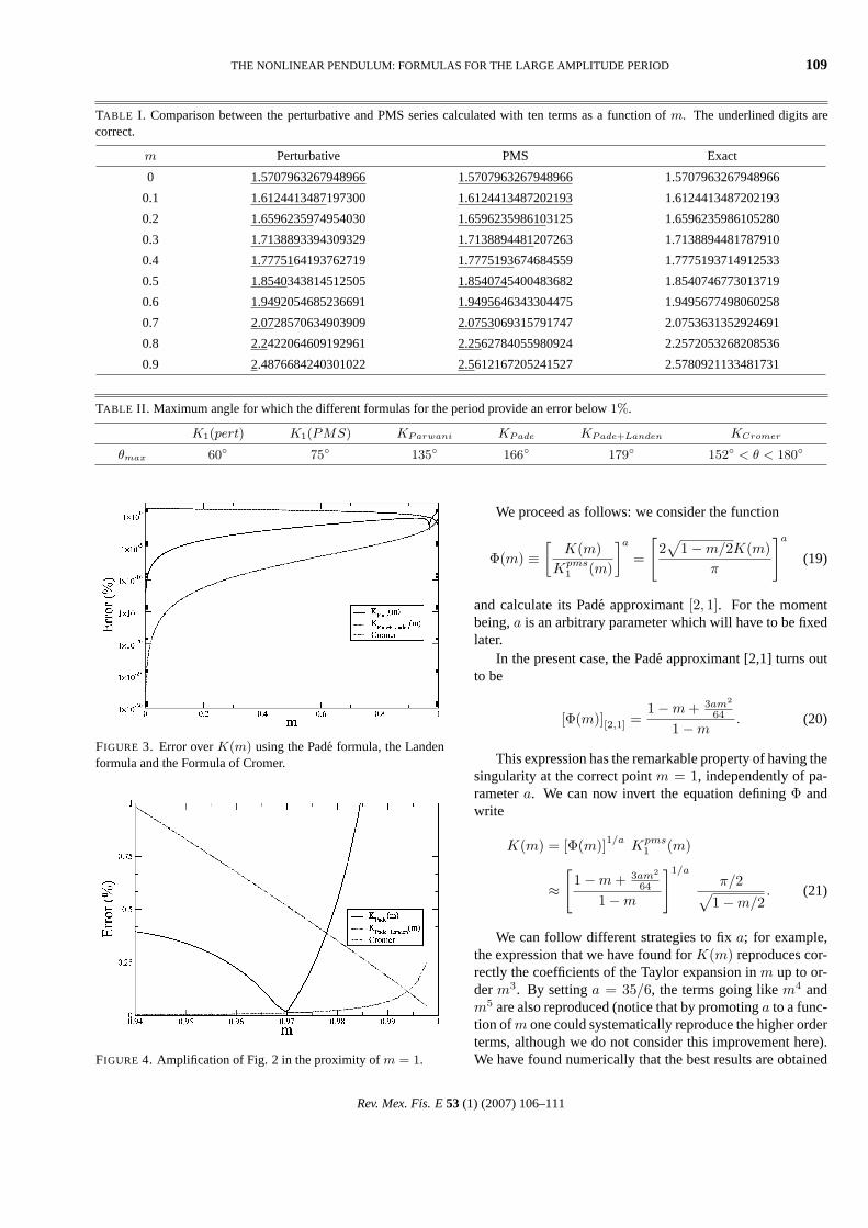
TABLE I. Comparison between the perturbative and PMS series calculated with ten terms as a function ofm. The underlined digits arecorrect.

m Perturbative PMS Exact

0 1.5707963267948966 1.5707963267948966 1.5707963267948966

0.1 1.6124413487197300 1.6124413487202193 1.6124413487202193

0.2 1.6596235974954030 1.6596235986103125 1.6596235986105280

0.3 1.7138893394309329 1.7138894481207263 1.7138894481787910

0.4 1.7775164193762719 1.7775193674684559 1.7775193714912533

0.5 1.8540343814512505 1.8540745400483682 1.8540746773013719

0.6 1.9492054685236691 1.9495646343304475 1.9495677498060258

0.7 2.0728570634903909 2.0753069315791747 2.0753631352924691

0.8 2.2422064609192961 2.2562784055980924 2.2572053268208536

0.9 2.4876684240301022 2.5612167205241527 2.5780921133481731

TABLE II. Maximum angle for which the different formulas for the period provide an error below1%.

K1(pert) K1(PMS) KParwani KPade KPade+Landen KCromer

θmax 60◦ 75◦ 135◦ 166◦ 179◦ 152◦ < θ < 180◦

FIGURE 3. Error overK(m) using the Pade formula, the Landenformula and the Formula of Cromer.

FIGURE 4. Amplification of Fig. 2 in the proximity ofm = 1.

We proceed as follows: we consider the function

Φ(m) ≡[

K(m)Kpms

1 (m)

]a

=

[2√

1−m/2K(m)π

]a

(19)

and calculate its Pade approximant[2, 1]. For the momentbeing,a is an arbitrary parameter which will have to be fixedlater.

In the present case, the Pade approximant [2,1] turns outto be

[Φ(m)][2,1] =1−m + 3am2

64

1−m. (20)

This expression has the remarkable property of having thesingularity at the correct pointm = 1, independently of pa-rametera. We can now invert the equation definingΦ andwrite

K(m) = [Φ(m)]1/aKpms

1 (m)

≈[

1−m + 3am2

64

1−m

]1/aπ/2√

1−m/2. (21)

We can follow different strategies to fixa; for example,the expression that we have found forK(m) reproduces cor-rectly the coefficients of the Taylor expansion inm up to or-derm3. By settinga = 35/6, the terms going likem4 andm5 are also reproduced (notice that by promotinga to a func-tion ofm one could systematically reproduce the higher orderterms, although we do not consider this improvement here).We have found numerically that the best results are obtained

Rev. Mex. Fıs. E53 (1) (2007) 106–111

110 P. AMORE, M. CERVANTES VALDOVINOS, G. ORNELAS, AND S. ZAMUDIO BARAJAS

for a ≈ 13/2, which gives us the remarkably simple formula

Kpade(m) =[1−m + 39

128m2

1−m

]2/13π/2√

1−m/2. (22)

This formula can still be drastically improved by us-ing the Landen transformation [13], which relates the valuestaken by the elliptic integral at different points:

K(m) =1

1 +√

mK

(4√

m

(1 +√

m)2

)(23)

and

K(m)=2(1−√1−m)

mK

((−2+2

√1−m+m)2

m2

). (24)

The first formula relates the value of the elliptic integralK(m) with the value at a larger point

m1(m) =4√

m

(1 +√

m)2;

the second formula relates the value of the elliptic integralK(m) with the value taken at a smaller point

m2(m) =(−2 + 2

√1−m + m)2

m2.

Equation (24) can be applied to any approximate expres-sion ofK(m) valid for smallm, changing it into an expres-sion which becomes valid for much larger values ofm. In-deed a repeated application of the transformation makes itpossible to obtain arbitrarily accurate values ofK(m) for anygiven value ofm. We have applied the Landen transforma-tion to our Eq. (22) and we have compared the error, definedas

|K(m)−Kapprox(m)|K(m)

× 100,

with the errors found using Eq. (22) and the equation ofCromer [7], valid form → 1, which is given by

KCromer(m) =12

log16

1−m. (25)

In Fig. 3 we have plotted the three errors observing thateven the simple formula (22) provides an excellent approxi-mation up to quite large values ofm. Indeed, in Fig. 4 wehave made an amplification of Fig. 3 close tom = 1 andseen that Eq. (22) provides an error smaller than 1% up to

m ≈ 0.986; the Landen improved formula, which howeveris as simple as the previous one, provides an error smallerthan 1% up tom ≈ 0.99999. We also notice that Eq. (25)performs better than our formula only form > 0.98, corre-sponding to an angleθ ≈ 164◦.

Another approximate formula for the period of the pen-dulum has also been derived recently by Parwani [6]:

KParwani =π

2

( √3

2 θ

sin√

32

)1/2

, (26)

providing good approximations for the period of the pendu-lum up to moderate values of the amplitude. In Table II, wehave calculated the value of the maximum angle for whicha maximum error of1% is obtained, using the different ap-proximations. Using our formula (22), we are able to reacha maximum angle of166◦, despite its simplicity, comparedwith the value of135◦ reached by Parwani.

4. Conclusions

In this paper we have derived a simple formula for the large-angle oscillations of the nonlinear pendulum, which com-pares quite favorably with other expressions found in the lit-erature and has the advantage of being based on a systematicapproach (and therefore of being improvable to any desiredlevel of accuracy) and of never involving special functions.In its present form our formula based, on the LDE and on thePade approximants, reaches a precision which is sufficient forall practical applications.

The main goal of the paper, however, was not to deriveanother approximate formula for the period of the pendulum.Although this formula is valuable and useful in practice, webelieve that far more valuable is the explanation to the readerto non-perturbative techniques such as the LDE or the Padeapproximants; these techniques are normally used in attack-ing more difficult problems in quite diverse areas of Physics,from classical and quantum mechanics to quantum field the-ory, and we believe that the pendulum can be used as a firstexample where a student can become familiarized with no-tions which are usually encountered much later in his studies.

Acknowledgments

P.A. acknowledges support of Conacyt grant no. C01-40633/A-1. P.A. and G.O. also acknowledge support ofFondo Ramon Alvarez Buylla of Colima University.

i. By looking back at Eq. (6) we see that physically this is relatedto the fact thatθ = π is a point of unstable equilibrium.

ii. The reader can convince himself that the “perturbative” series,Eq. (8), corresponds to Eq. (14) takingλ = 0.

1. W.P. Ganley,Am. J. Phys.53 (1995) 73.

2. R.B. Kidd and S.L. Fogg,Phys. Teach.40 (2003) 81.

3. M.I. Molina, Phys. Teach.35 (1997) 489.

4. P. Amore and R.A. Saenz,Europhysics Letters70 (2005) 425.

Rev. Mex. Fıs. E53 (1) (2007) 106–111

THE NONLINEAR PENDULUM: FORMULAS FOR THE LARGE AMPLITUDE PERIOD 111

5. B.Wu and P. Li,Meccanica36 (2001) 167.

6. R. Parwani,European Journal of Physics25 (2004) 37.

7. A. Cromer,Americal Journal of Physics63 (1995) 112.

8. L.M. Burko, European Journal of Physics24 (2002) 125.

9. A. Duncana and M. Moshe,Phys. Lett. B125 (1998) 352;A.Okopinska, Phys. Rev. D35 (1987) 1835; G. Krein,D.P. Menezes, and M.B. Pinto,Phys. Lett. B370 (1996) 5;M.P. Blencowe and A.P. Korte,Phys. Rev. B56 (1997) 9422;H.F. Jones, P. Parkin, and D. Winder,Phys. Rev. D63 (2001)125013; J.L. Kneur, M.B. Pinto, and R.O. Ramos,Phys. Rev.Lett. 89(2002) 210403; A. Pelster, H. Kleinert, and M. Schanz,Phys. Rev. E67 (2003) 016604.

10. G.A. Arteca, F.M. Fernandez, and E.A. Castro,Large orderperturbation theory and summation methods in quantum me-chanics (Springer, Berlin, Heidelberg, New York, London,Paris, Tokyo, Hong Kong, Barcelona, 1990).

11. H. Kleinert, Path Integrals in Quantum Mechanics, Statisticsand Polymer Physics, 3rd edition (World Scientific Publishing,2004).

12. P.M. Stevenson,Phys. Rev. D23 (1981) 2916.

13. Handbook of Mathematical Functions, edited by M.Abramowitz and I.A. Stegun (Dover, New York, 1965).

Rev. Mex. Fıs. E53 (1) (2007) 106–111