the notation of dynamic levels in the … · the late mixed pieces by luigi nono make an extensive...
TRANSCRIPT
THE NOTATION OF DYNAMIC LEVELS IN THE
PERFORMANCE OF ELECTRONIC MUSIC
Carlo Laurenzi Marco Stroppa
Ircam, Paris
Hochschule für Musik und
Darstellende Kunst, Stuttgart
ABSTRACT
The “sound diffusion” (or “sound projection”), that is,
“the projection and the spreading of sound in an acoustic
space for a group of listeners”[1], of works for solo
electronics or for acoustic instruments and electronics (so
called, “mixed pieces”), has always raised the issue of
notating the levels to be reproduced during a concert or
the correct balance between the electronics and the in-
struments.
If, in the last decades, some attempts were made by
few composers or computer-music designers, mostly in
the form of scores, none of these managed to establish a
common practice. In addition, little theoretical work has
been done so far to address the performative aspects of a
piece, that is, to provide just the useful information to the
person in charge of the sound diffusion.
Through the discussion of three historical examples
and the analysis of two experiences we developed, we
will try to identify some possibly general solutions that
could be adopted independently on the aesthetic or tech-
nological choices of a given piece.
1. PRELIMINARY CONSIDERATIONS
The notation of electronic music has generated only few,
often partial, essays. Most of the literature is either quite
theoretical [2], or it delves into the automated translation
of electronic sounds into a sort of graphical score, such as
in [3]. These experiments were mainly aimed at provid-
ing ways to analyse purely electronic pieces more deeply
than when simply listening to them, to account for the
compositional process, or as an attempt to digitally pre-
serve and archive cultural assets [4].
To our knowledge, little theoretical work has been
done to tackle the more general issue of how to notate
dynamic levels on a score that is to be read by the com-
puter music performer (CMP) who will perform the elec-
tronics during a concert. The CMP does not need to be
the composer or the first performer of the piece.
Although this task could be programmed on a com-
puter and automated during the concert, a much better
result can be achieved when doing it by ear. The listening
and musical skills of a human being are, in fact, still
much superior to what a machine can realize. The sound
diffusion can be adapted to the acoustics of the hall, the
properties of the loudspeakers, the whole audio system,
the relationship between these and the acoustic image of
the instruments on stage, whether they are amplified or
not, and, finally, to the emotional reaction of the audi-
ence.
As a consequence, most of the time, the dynamic lev-
els are controlled by ear (and by hand) by the CMP or the
composer. Often they are only roughly sketched on the
score. If a faithful recording will certainly help as a refer-
ence, the information is usually insufficient, especially in
the case of particular spatial configurations that cannot be
reproduced by a stereo recording.
Therefore, the most effective solution is to notate all
the information about the sound diffusion directly on the
score that will be used during the performance.
To delimit our scope, we will concentrate on the nota-
tion of dynamic levels and will not tackle the issue of
notating other parameters used for real-time sound pro-
cessing, such as, for instance, the transposition factor of a
harmonizer.
1.1 Levels vs. loudness vs. musical dynamics
Objectively, levels are normally expressed in decibels, a
logarithmic unit that is related to the ratio between the
value of a given and of a reference sound pressure (usual-
ly, either the threshold of audibility, or the maximum
available value in a given system)1.
However, there are other ways to do it: from the point
of view of the perception, the dynamic levels are called
“loudness” and use phons (a unit that takes into account
1 See http://en.wikipedia.org/wiki/Decibel (accessed
3/10/2015)
Copyright: © 2015 Carlo Laurenzi et al. This is an open-access article
distributed under the terms of the Creative Commons Attribu-
tion License 3.0 Unported, which permits unrestricted use,
distribution, and reproduction in any medium, provided the original
author and source are credited.

the psycho-acoustic effect of the equal-loudness curves
ISO 226:2003)2; from a musical point of view, levels are
called “dynamics” and use symbols such as ff, mf, pp.
Three important factors need to be taken into account:
first, the same musical dynamics played by different
instruments, or in different ranges of the same instrument,
might yield different objective or perceptual levels; sec-
ond, choices of interpretation play an important role and
produce different absolute levels for the same musical
dynamics, as pointed out in [5]3; third, the perception of
an acoustic instrument’s crescendo is always associated
to the production of a richer and broader spectrum, that
is, to a shift of the spectral “centre of gravity” toward a
higher value. These spectral aspects differ specifically
from each instrument and can be easily demonstrated by
recording three sound files at three different dynamics
(say, pp, mf, ff), clean them from background noises and
finally normalize them. Even though they have the same
maximum amplitude, their dynamics can be easily and
correctly identified.
Hence, simply raising a fader will not be sufficient to
convey a real feeling of crescendo, but rather of a sound
getting closer. When notating levels into a performance
score, which unit should be used: dBs, loudness or musi-
cal dynamics?
1.2 Level changes
The notation of levels changes (usually, albeit incorrect-
ly, called crescendo or diminuendo) can use several strat-
egies, like, for instance, crescendo or diminuendo sym-
bols to illustrate the change between adjacent values
(Figure 1a), simple straight lines, either with (Figure 1c)
or without (Figure 1b) a reference scale of amplitude
ranges for each level in the score, or, finally, simple small
upward or downward arrows, eventually with some abso-
lute values (Figure 1d-e).
Figure 1. Different ways of notating changes of levels.
2 See http://en.wikipedia.org/wiki/Phon (accessed
3/10/2015) 3 “The absolute meanings of dynamic markings change, depend on the
intended (score defined) and projected (actual) dynamic levels of the
surrounding context”, [5] abstract.
These strategies clearly suggest that a compromise be-
tween space or information economy and score readabil-
ity need to be found. Their usage also depends on the
nature of the required movements: simply raising a fader
to a given static level does not require the same precision
as a jagged change over a longer period of time.
2. THREE HISTORICAL EXAMPLES
2.1 K. Stockhausen: Kontakte
Kontakte [6] was originally a 4-channel electronic piece
composed in 1958-60 by Karlheinz Stockhausen. Soon
after, the composer wrote a version for piano, percussion
and the same 4-channel electronic material. The original
score shows one of the first, composer-written, attempts
to graphically notate the electronic material using uncon-
ventional, graphical signs. The second edition, published
in 2008, adds some hints at the balance between the am-
plified instruments and the electronics. In Figure 2, a +
above the piano means that the level of the amplification
of that instrument should be raised until N (normal) is
found.
Figure 2. Kontakte (p. 1 excerpt, © Stockhausen Stiftung für Musik,
Kürten, by kind permission).
Some gestures can be notated, but are hard to realize
by hand, as they are very short, as the sudden reinforce-
ment of the, respectively, electronics and marimba (+) in
Figure 3.

Figure 3. Kontakte (p. 17, excerpt, © Stockhausen Stiftung für Musik,
Kürten, by kind permission ).
On one occasion (Figure 4, page 32), after lowering
the electronics (-), the composer explicitly asks for the
channels II and IV to be reduced by ca. 5dB, because of a
problem of balance in the original mixing, while the
channels I and III remain at the N level.
Figure 4. Kontakte (p. 32, excerpt, © Stockhausen Stiftung für Musik,
Kürten, by kind permission ).
To summarize: if the positions and panning of the mi-
crophones are very clearly specified in the technical notes
that come with the score, information about the sound
diffusion, added only in the second edition, is limited to
+, - and N (normal) signs. However, this is already suffi-
cient to have an idea of the sound diffusion.
2.2 L. Nono: A Pierre / Omaggio a György Kurtàg
The late mixed pieces by Luigi Nono make an extensive
usage of simple, but continuous live-electronic treat-
ments. Since the original score totally lacked information
about the electronics, André Richard and Alvise Vidolin,
who assisted the composer during several performances,
together with Ricordi’s editor Marco Mazzolini, em-
barked on the ambitious task of notating both the elec-
tronic setup and the sound diffusion in such a detailed
way, that other people might play the piece without re-
quiring other information than what is marked in the
score.
In A Pierre [7], for bass flute, double bass clarinet and
electronics (4 loudspeakers), the dynamics are marked
using a mixture of the strategy shown in Figure 1b and
musical dynamics, in spite of the fact, that the latter re-
quire both a level and a spectral change to be correctly
perceived (Figure 5).
Figure 5. Level changes in L. Nono’s A Pierre.
In another work, Omaggio a György Kurtàg [8], for
contralto, flute, clarinet, tuba and electronics (6 loud-
speakers), a further distinction is made between micro-
phone faders (M1, M2, etc.), mainly used for sending the
sound to the treatments, and output faders (L1-6). In
addition, the portion of sound that needs to be recorded
by a treatment is greyed in the score (Figure 6).
The notation is adequate to the needs of the composer,
and many aspects of it can also be generalized.
2.3 P. Boulez: Anthèmes 2
The Universal Edition performance score of Pierre Bou-
lez’s Anthèmes 2 [9], for violin and electronics, was real-
ized by the composer’s musical assistant at Ircam, An-
drew Gerzso. Up to now, it is one of the rare examples
that features a complete and detailed notation of the elec-
tronics (using dedicated staves for each electronic part or
treatment). Together with the extensive technical manual,
the score allows for the re-constitution of the electronics
even without the original patch (Figure 7).

Figure 6.L. Nono’s Omaggio a György Kurtàg (p. 8, © Casa Ricordi,
by kind permission).
Figure 7. Beginning of P. Boulez’s Anthèmes 2 (© Universal Edition,
Wien, by kind permission).
Surprisingly, there are almost no indications about
dynamic levels: all the information is, in fact, contained
in the Max patch for the piece. The balance between the
violin and the electronics is explained in the technical
manual and set in the patch. Levels are automated and
changed globally, by recalling a different preset for each
movement. The presets should be revised during the
rehearsals, but, during the concert, only minor adjust-
ments might be required from time to time.
This approach is related to those mixed pieces in
which it is mainly the acoustic musician who is responsi-
ble for the amplitude of the real-time treatments; the
interaction with the CMP, though still important, is there-
fore less crucial, the work being rather structured around
pitches and timbral articulations.
It is therefore clear, that in Anthèmes 2 the dynamic
levels of the electronics play a different role as, for in-
stance, in Nono’s works, and, hence, do not need to be
notated in the same detailed way.
3. HYPOTHESES
3.1 The case of Spirali (1987-88)
3.1.1 Setup
In Marco Stroppa’s Spirali (Spirals) [10], for string quar-
tet projected into the space, the electronics is constituted
by a unique setup, exclusively made of six simultaneous,
always active, types of reverb. Placed on stage as far as
possible from the audience, the acoustic quartet, closely
miked, is amplified and only heard through 4 or 6 loud-
speakers around the audience, depending on the size of
the hall (Figure 8).
Figure 8. Spirali: setup with 6 loudspeakers.
Originally performed with analog equipment, Spirali
was ported at Ircam by Serge Lemouton in 2005 as a Max
patch with 18 control faders. The performance of the
electronic part was a terribly virtuoso and risky undertak-
ing and required an extensive study and clear skills! In
2013, Carlo Laurenzi integrated the Antescofo language4
to the patch and automated some controls. This resulted
in a more effective interface, with only 13 faders to move
during the performance, although it is still quite challeng-
ing to perform.
4See http://repmus.ircam.fr/antescofo/documents
for an abundant bibliography about Antescofo (accessed 1/28/2015).
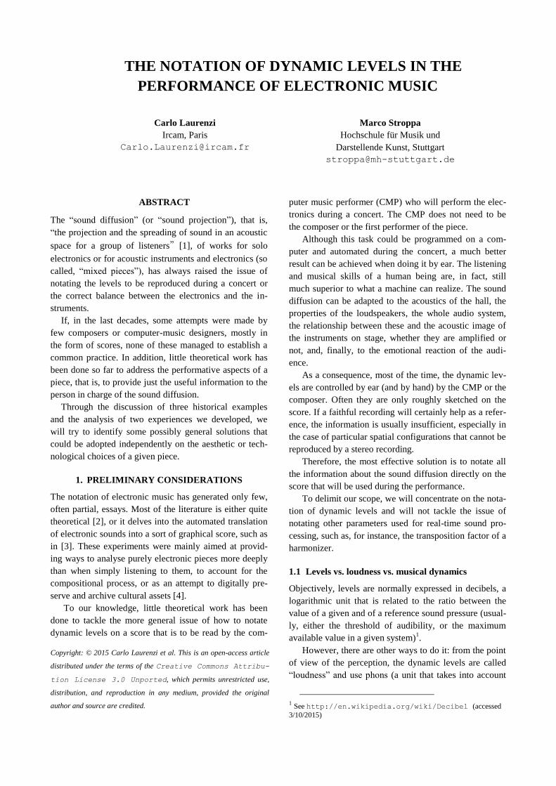
3.1.2 Spatial taxonomy: space families
During the composition, Stroppa organised space into a
personal taxonomy made of three space families: points
(P), surfaces (S) and diffused space (D). He then related
the six reverbs and the amplified instruments to it. Points
correspond to the direct amplification of an instrument, to
which correspond only one or two loudspeakers depend-
ing on the setup (Figure 9)
Figure 9. Points: double amplified quartet (6 loudspea-kers)
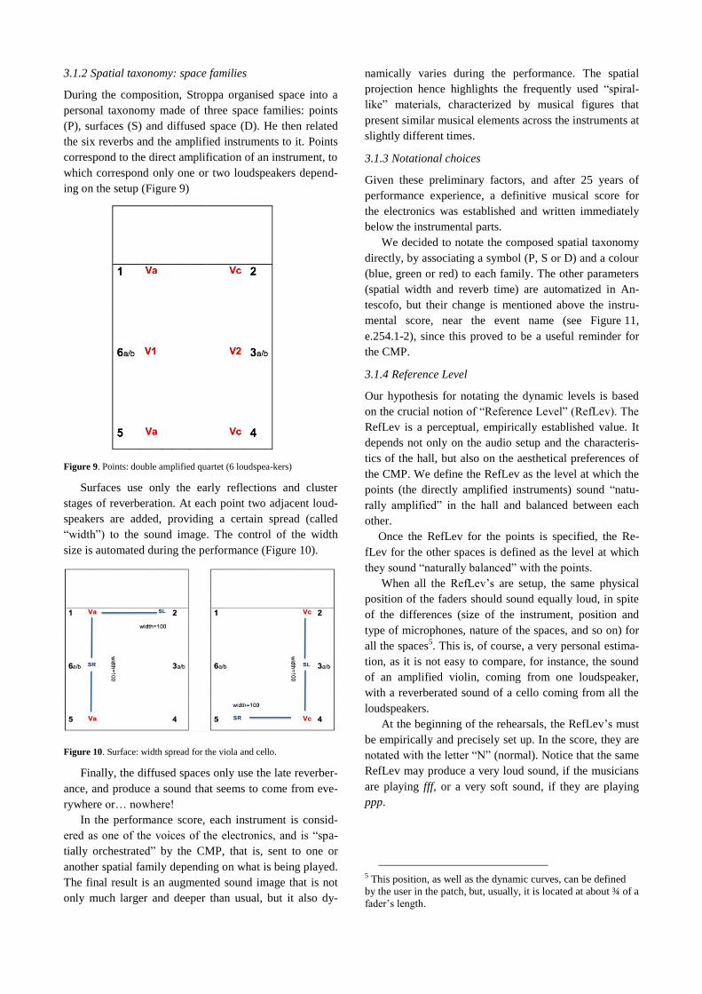
Surfaces use only the early reflections and cluster
stages of reverberation. At each point two adjacent loud-
speakers are added, providing a certain spread (called
“width”) to the sound image. The control of the width
size is automated during the performance (Figure 10).
Figure 10. Surface: width spread for the viola and cello.
Finally, the diffused spaces only use the late reverber-
ance, and produce a sound that seems to come from eve-
rywhere or… nowhere!
In the performance score, each instrument is consid-
ered as one of the voices of the electronics, and is “spa-
tially orchestrated” by the CMP, that is, sent to one or
another spatial family depending on what is being played.
The final result is an augmented sound image that is not
only much larger and deeper than usual, but it also dy-
namically varies during the performance. The spatial
projection hence highlights the frequently used “spiral-
like” materials, characterized by musical figures that
present similar musical elements across the instruments at
slightly different times.
3.1.3 Notational choices
Given these preliminary factors, and after 25 years of
performance experience, a definitive musical score for
the electronics was established and written immediately
below the instrumental parts.
We decided to notate the composed spatial taxonomy
directly, by associating a symbol (P, S or D) and a colour
(blue, green or red) to each family. The other parameters
(spatial width and reverb time) are automatized in An-
tescofo, but their change is mentioned above the instru-
mental score, near the event name (see Figure 11,
e.254.1-2), since this proved to be a useful reminder for
the CMP.
3.1.4 Reference Level
Our hypothesis for notating the dynamic levels is based
on the crucial notion of “Reference Level” (RefLev). The
RefLev is a perceptual, empirically established value. It
depends not only on the audio setup and the characteris-
tics of the hall, but also on the aesthetical preferences of
the CMP. We define the RefLev as the level at which the
points (the directly amplified instruments) sound “natu-
rally amplified” in the hall and balanced between each
other.
Once the RefLev for the points is specified, the Re-
fLev for the other spaces is defined as the level at which
they sound “naturally balanced” with the points.
When all the RefLev’s are setup, the same physical
position of the faders should sound equally loud, in spite
of the differences (size of the instrument, position and
type of microphones, nature of the spaces, and so on) for
all the spaces5. This is, of course, a very personal estima-
tion, as it is not easy to compare, for instance, the sound
of an amplified violin, coming from one loudspeaker,
with a reverberated sound of a cello coming from all the
loudspeakers.
At the beginning of the rehearsals, the RefLev’s must
be empirically and precisely set up. In the score, they are
notated with the letter “N” (normal). Notice that the same
RefLev may produce a very loud sound, if the musicians
are playing fff, or a very soft sound, if they are playing
ppp.
5 This position, as well as the dynamic curves, can be defined
by the user in the patch, but, usually, it is located at about ¾ of a
fader’s length.
3.1.5 Level changes
Once the RefLev’s are defined, all the other levels are
notated as a dynamic difference with respect to them and
marked with 1 to 3 “+” or “-” (that is, for instance, “+++”
or “- -”). They are defined as three clearly different and
perceptible dynamic layers: one +/– means slightly loud-
er/softer than the RefLev, two +/– means clearly louder
or softer, three +/– are extreme levels, from macro-
amplified to barely amplified.
These levels are not absolute, but rather correspond to
perceptual areas, and will, therefore, vary during the
piece as a function of what kind of music is being per-
formed. They indicate subjectively different “steps” in
the amplification process: seven dynamic steps were
considered as necessary and sufficient to accurately per-
form the sound diffusion of Spirali.
Since the changes between levels are not very com-
plex, the traditional signs of cresc. and dim. were adopt-
ed, because they are expressive, use a space in the score
that does not depend on the dynamic range and allow for
the notation of a duration (see Figure 11).
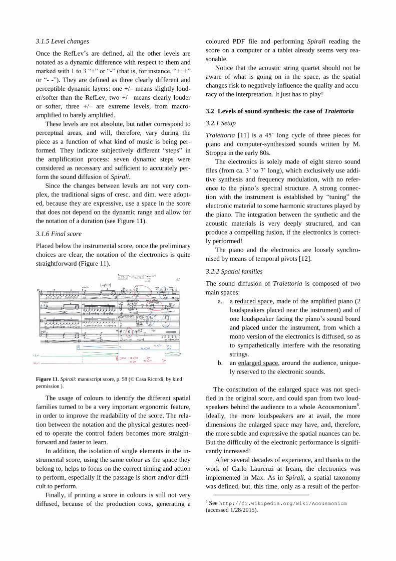
3.1.6 Final score
Placed below the instrumental score, once the preliminary
choices are clear, the notation of the electronics is quite
straightforward (Figure 11).
Figure 11. Spirali: manuscript score, p. 58 (© Casa Ricordi, by kind
permission ).
The usage of colours to identify the different spatial
families turned to be a very important ergonomic feature,
in order to improve the readability of the score. The rela-
tion between the notation and the physical gestures need-
ed to operate the control faders becomes more straight-
forward and faster to learn.
In addition, the isolation of single elements in the in-
strumental score, using the same colour as the space they
belong to, helps to focus on the correct timing and action
to perform, especially if the passage is short and/or diffi-
cult to perform.
Finally, if printing a score in colours is still not very
diffused, because of the production costs, generating a
coloured PDF file and performing Spirali reading the
score on a computer or a tablet already seems very rea-
sonable.
Notice that the acoustic string quartet should not be
aware of what is going on in the space, as the spatial
changes risk to negatively influence the quality and accu-
racy of the interpretation. It just has to play!
3.2 Levels of sound synthesis: the case of Traiettoria
3.2.1 Setup
Traiettoria [11] is a 45’ long cycle of three pieces for
piano and computer-synthesized sounds written by M.
Stroppa in the early 80s.
The electronics is solely made of eight stereo sound
files (from ca. 3’ to 7’ long), which exclusively use addi-
tive synthesis and frequency modulation, with no refer-
ence to the piano’s spectral structure. A strong connec-
tion with the instrument is established by “tuning” the
electronic material to some harmonic structures played by
the piano. The integration between the synthetic and the
acoustic materials is very deeply structured, and can
produce a compelling fusion, if the electronics is correct-
ly performed!
The piano and the electronics are loosely synchro-
nised by means of temporal pivots [12].
3.2.2 Spatial families
The sound diffusion of Traiettoria is composed of two
main spaces:
a. a reduced space, made of the amplified piano (2
loudspeakers placed near the instrument) and of
one loudspeaker facing the piano’s sound board
and placed under the instrument, from which a
mono version of the electronics is diffused, so as
to sympathetically interfere with the resonating
strings.
b. an enlarged space, around the audience, unique-
ly reserved to the electronic sounds.
The constitution of the enlarged space was not speci-
fied in the original score, and could span from two loud-
speakers behind the audience to a whole Acousmonium6.
Ideally, the more loudspeakers are at avail, the more
dimensions the enlarged space may have, and, therefore,
the more subtle and expressive the spatial nuances can be.
But the difficulty of the electronic performance is signifi-
cantly increased!
After several decades of experience, and thanks to the
work of Carlo Laurenzi at Ircam, the electronics was
implemented in Max. As in Spirali, a spatial taxonomy
was defined, but, this time, only as a result of the perfor-
6 See http://fr.wikipedia.org/wiki/Acousmonium
(accessed 1/28/2015).

mances with several different audio systems and configu-
rations, and not when the piece was composed. Then, a
suggested, standard taxonomy for the sound diffusion
was defined: 7 families of spaces (totalling 11 main loud-
speakers, see Figure 12). Each family is given a name and
a symbol and is controlled by one fader: FC (Front Cen-
tre), Pf (Piano), U (Under the piano), F[R/L] (Front
[Left/Right]), M[L/R] (Middle), R[L/R] (Rear), RC (Rear
Centre). It is for this taxonomy that a new notation was
established.
3.2.3 Notational choices
When Traiettoria…deviata was first published, it was
provided with a unique, exhaustive notation of the syn-
thetic sounds [13], a simple notation of the two main
diffusion spaces (M=under the piano, D/S = left/right)
and a double time staff (Tpo, Figure 13). The absolute
times placed in the middle of the time staves are temporal
pivots, the other markings belong to either the piano or
the electronics7.
Figure 12. Traiettoria: standard audio setup.
Notice that the traditional cresc/dim signs are used,
but that the composer explicitly asks for a shift of the
7 Since the electronics has to be tuned to the piano’s A by
slightly changing the reading speed, these times are not meant
to be strictly followed, but to serve as an indication. Because of
this, the usage of a stopwatch would simply not be precise
enough. None of the pianists with whom we have worked ever
used one during a concert.
spectral centre of gravity toward a higher region together
with the movement of the faders. This was done with a
HP-filter placed on the electronics’ stereo input moved
together with the fader.
As impressive as it may look, this notation proved not
to be very practical for the sound diffusion. It contained
too much information that was not required during a
concert and too little information regarding the actual
spreading of sound.
Finally, its “orchestral” appearance made it difficult
for the pianist to grasp which sounds are easier to hear,
and therefore to visually identify the essential cues corre-
sponding to the temporal pivots to which the performance
had to be synchronised. A more pragmatic and expres-
sively efficient solution had to be found.
3.2.4 Reference Level
Based on our experience with Spirali, we defined a Re-
fLev for Traiettoria as the subjective level at which the
piano sounds “naturally amplified”, and the electronics
“naturally balanced” with it. However, here, it did not
seem necessary to explicitly mark it in the score (with N).
Three degrees of +/- indicate, as in Spirali, six perceptu-
ally different dynamics for the piano or the electronics.
Figure 13. Traiettoria…deviata: original version, p. 21 (© Casa Ri-
cordi, by kind permission).
During the performance of Traiettoria, the most diffi-
cult task is to find a musical balance between the sound
in the hall and the piano (and some electronics) on stage.
How to compare, for instance, an electronic sound com-
ing from behind the audience with the piano? When the
same level is indicated in the score, it is the task of the
CMP to (subjectively) estimate the correct sound image
and intensity.
3.2.5 Composition of the sound diffusion
Even though, in theory, there are as many ways to per-
form the sound diffusion of Traiettoria as there are con-
certs, the practical experience showed that some strate-
gies were more musical and tended to be regularly re-
peated.
In the tradition of the acousmatic music, the sound
diffusion is thought as a real orchestration of the electron-
ic voices over a moving, imaginary space. Stroppa com-
posed a precise hierarchy that organises not only the
audio setup, but also the spatial form of Traiettoria.
For instance, Traiettoria…deviata starts with a barely
amplified piano that gets increasingly louder, that is,
more amplified. This yields a larger and larger sound
image. When the electronics joins in, it fades into the
piano’s decaying resonance, and comes out only from U
(see 3.2.2). Little by little, the constricted space of the
electronics opens up to the Pf and the F groups, thus
unfolding its image around the piano. It is only at 1’57
that the R group is activated. A detailed analysis of the
spatial form of the sound diffusion of Traiettoria is be-
yond the score of this text, but it is important to remark
that, since it is an important part of the composition of the
piece, it needs to be precisely and correctly notated.
Each spatial group is represented by one fader on the
control interface8 and by one vertical position in the
score. Since each group is identified by a letter, it needs
to appear in the score only when it is active. In this way,
the usage of the space within the page is more efficient.
3.2.6 Level changes
It did not seem necessary to find a more refined way to
notate level changes than what was used in Spirali. In the
few moments, where a random spread is needed, it is
directly asked for by some text written in the score and
each CMP can freely choose how to perform it.
3.2.7 Main/Secondary loudspeaker(s)
Together with the taxonomy explained in 3.2.2, the sound
diffusion of Traiettoria extends the concept of loud-
speaker. Each spatial family, identified by a letter, repre-
sents the “main loudspeaker”, defined as the loudspeaker
8 A MIDI mixer or an OSC-driven device, such as an iPad.
(or the couple of loudspeakers) that is heard as the main
source of diffusion.
It is, however, always possible, depending on the
characteristics of the hall or personal taste, to enlarge the
focus of a single loudspeaker by diffusing the same elec-
tronic material into nearby loudspeakers (called “second-
ary loudspeakers”), at a softer level, so as to change the
acoustic image of the main loudspeaker, without directly
perceiving the other ones.
Being rather a performer’s aesthetical choice, we de-
cided not to notate this sound-diffusion technique, except
when it had a compositional role.
3.2.8 Score
The final score is still under preparation, but concrete
experiments and current sketches showed that simply
notating the levels above the piano part was not sufficient
to achieve a good performance and efficiently learning
from the score.
After some tests, we found that adding a sonogram
window of a mono mix of the synthetic sounds on top of
the page was the best choice to correctly perform the
electronics.
Even if a sonogram is very concise and cannot pre-
cisely represent pitched and rhythmic material, the most
important temporal elements are still clearly identifiable
and help both performers to follow the spectro-
morphological unfolding of the electronics. And if some
special pitch or rhythmic structures need to be marked, it
is always possible to locally add this information on the
sonogram or between it and the dynamic levels.
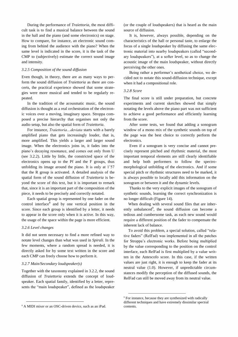
Thanks to the very explicit images of the sonogram of
synthetic sounds, learning the correct synchronization is
no longer difficult (Figure 14).
When dealing with several sound files that are inher-
ently unbalanced9, the sound diffusion can become a
tedious and cumbersome task, as each new sound would
require a different position of the fader to compensate the
inherent lack of balance.
To avoid this problem, a special solution, called “rela-
tive faders” (RelFad) was implemented in all the patches
for Stroppa’s electronic works. Before being multiplied
by the value corresponding to the position on the control
interface, each RelFad is first multiplied by a value writ-
ten in the Antescofo score. In this case, if the written
values are just right, it is enough to keep the fader at its
neutral value (1.0). However, if unpredictable circum-
stances modify the perception of the diffused sounds, the
RelFad can still be moved away from its neutral value.
9 For instance, because they are synthesized with radically
different techniques and have extremely dissimilar spectral
contents.

As a consequence, the movement of faders during the
performance is greatly reduced, and the performance
itself becomes more ergonomic and gesture-effective.
The written values lay half way between the realm of the
composition and of the interpretation and can always be
very easily changed. One might also imagine to have
presets of good values for different acoustical situations.
Since they were implemented, RelFad’s have greatly
improved the task of learning to perform the electronics
of a mixed piece, and have helped to spread the sound
diffusion technique to a larger community of CMP’s.
Figure 14. Traiettoria : sketch of the new electronic score. Relative
faders
4. CURRENT STATE
The notation of dynamic levels in the performance scores
of Spirali and Traiettoria was inspired by the late Nono’s
works, but the musical context is very different and has a
totally diverse goal.
In Nono’s works the notation was intended to approx-
imately indicate the behaviour of the levels, in order to
provide a schematic structure for the performance of
pieces which allowed for a certain degree of improvisa-
tion from both the instrumental and electronic parts.
Stroppa, on the other hand, intends to confer a much
higher responsibility to role of the CMP, who is required
to possess a performance skill comparable to that of an
instrumentalist. For this reason, the performance score
must contain all the information needed to interpret the
piece and accurately represent the time relationships
between the acoustic instrument(s) and the electronics.
It is obvious that such a detailed performance score
needs some time to be learnt and practiced.
Finally, this score may also have the crucial function,
not only to effectively transmit precise information about
the sound diffusion to other CMP’s, but especially to
make it possible to understand how to render a complex
orchestration of synchronized spatial events between
electronics and instruments.
Due to the complexity of the music and the amount of
actions involved in the sound diffusion, learning the score
by heart rapidly became a necessity. However, the per-
formance score was still extremely useful during the
learning phase and the rehearsals.
5. CONCLUSIONS
Our experience has shown that it is possible to find gen-
eralized and efficient symbols to notate the sound diffu-
sion of electronic works, if it is not automated.
Our first step was to identify a spatial taxonomy adapted
to a given piece, in order to find an intermediate layer of
notation between the compositional concepts, the perfor-
mance needs and the physical audio setup.
The next step was to define the meaning and the value of
a RefLev for each situation and to notate all the other
relative dynamic changes with respect to this subjective
value. Introducing RelFad’s also greatly improved the
gestural aspects of a performance.
Our next step will be to extend this experience to the
control of real-time treatments.
Acknowledgments
This research was partially made during Stroppa’s sab-
batical leave from the Hochschule für Musik und Darstel-
lende Kunst in Stuttgart.
6. REFERENCES
[1] L. Austin, “Sound Diffusion in Composition and
Performance: An Interview with Denis Smalley” in
Computer Music Journal, vol. 24, no. 2, pp. 10–21,
2000.
[2] H. Eimert, F. Enkel, and K. Stockhausen, “Fragen
der Notation Elektronischer Musik” in Technische
Hausmitteilungen des Nordwestdeutschen
Rundfunks, vol. 6, pp. 52-54, 1954.
[3] G. Haus, “EMPS: A System for Graphic
Transcription of Electronic Music Scores,” in
Computer Music Journal, vol. 7, no. 3, pp. 31–36,
1983.
[4] N. Bernardini, A. Vidolin, “Sustainable Live
Electro-acoustic Music”, in Proceedings of the

International Sound and Music Computing
Conference, 2005. http://server.smcnetwork.org/files/proc
eedings/2005/Bernardini-Vidolin-SMC05-
0.8-FINAL.pdf (accessed Jan. 28, 2015)
[5] K. Kosta, O. F. Bandtlow, E. Chew: “Practical
Implications of Dynamic Markings in the Score: Is
piano always piano?", in Proceedings of Audio
Engineering Society 53rd International Conference,
London, 2014.
[6] K. Stockhausen, Kontakte, Stockhausen Stiftung für
Musik, Kürten, Germany, 2008
(www.karlheinzstockhausen.org).
[7] L. Nono, A Pierre. Dell’azzurro silenzio, inquietum,
Casa Ricordi, Milano, 1985
[8] L. Nono, Omaggio a György Kurtàg, Casa Ricordi,
Milano, 1983.
[9] P. Boulez, Anthèmes 2, Universal Edition, Wien,
1997.
[10] M. Stroppa, Spirali, Casa Ricordi, Milano, 1988.
[11] M. Stroppa, Traiettoria…deviata, Dialoghi,
Contrasti, from Traiettoria, Casa Ricordi, Milano,
1982-88.
[12] J. Duthen, M. Stroppa, “Une Représentation de
Structures Temporelles par Synchronisation de
Pivots”, in Proceedings of the Symposium: Musique
et Assistance Informatique, Marseille, pp. 305-322,
1990.
[13] M. Stroppa, “Un Orchestre Synthétique: Remarques
sur une Notation Personnelle”, in Le timbre:
Métaphores pour la Composition, J.B. Barrière Ed.,
Editions C. Bourgois, Paris, pp. 485-538, 1991.