The Numerical Integration of ChemicalReaction Rate Laws Using Computer

Spreadsheets

Eric L. KemerSt. Andrew's School

Middletown, DE 19709

General rate laws for chemical reactions can be solvedquantitatively using a simple numerical integration techniqueknown as Euler’s Method. When executed on a computerspreadsheet program, this method provides students with apowerful interactive tool for modeling chemical reaction kineticsand exploring the underlying dynamics of equilibrium.

†

aA + bB ´ cC + dD

†

Rr = + 1a

d A[ ]dt

= + 1b

d B[ ]dt

= - 1c

d C[ ]dt

= - 1d

d D[ ]dt

†

Rf = - 1a

d A[ ]dt

= - 1b

d B[ ]dt

= + 1c

d C[ ]dt

= + 1d

d D[ ]dt

†

Rf = k f A[ ]n B[ ]m

†

Rr = kr C[ ] r D[ ]s

†

Rnet = Rf - Rr = k f A[ ]n B[ ]m- kr C[ ]r D[ ]s

†

Q(t) =C[ ]c D[ ]d

A[ ]a B[ ]b

Forward and Reverse Reaction Rates Defined

†

limtƕ

Rnet = 0

Chemical Equilibrium

Reaction Quotient

General Reaction

Forward and Reverse Reaction Rate Laws

Net Reaction Rate Law in for a Closed System

†

kr = Ar exp DH - EA

RTÊ

Ë Á

ˆ

¯ ˜

†

kf = Af exp -EA

RTÊ

Ë Á

ˆ

¯ ˜

Arrhenius Equations for Rate Constants

†

limtƕ

Q = Keq

†

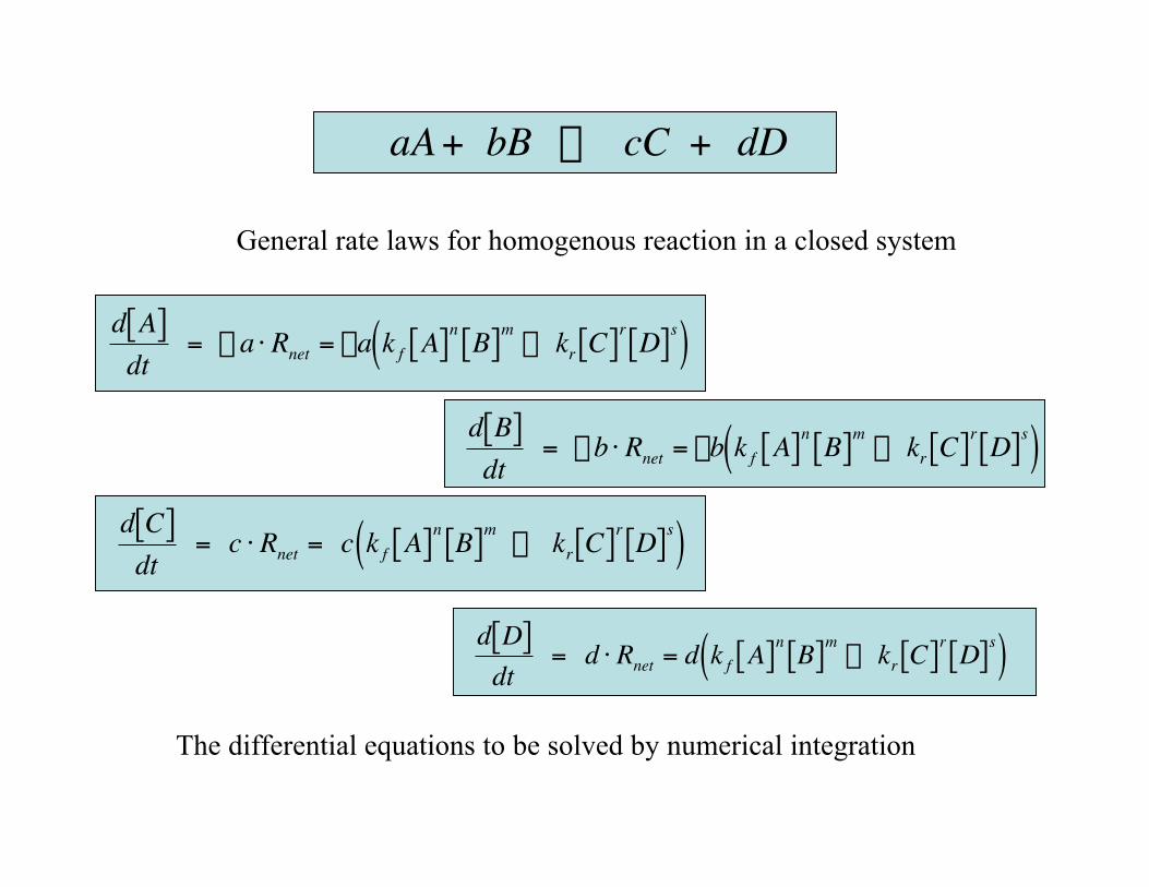
aA + bB ´ cC + dD

†

d D[ ]dt

= d ⋅ Rnet = d k f A[ ]n B[ ]m- kr C[ ]r D[ ]s( )

†

d A[ ]dt

= - a ⋅ Rnet = -a k f A[ ]n B[ ]m- kr C[ ]r D[ ]s( )

†

d B[ ]dt

= - b ⋅ Rnet = -b k f A[ ]n B[ ]m- kr C[ ]r D[ ]s( )

†

d C[ ]dt

= c ⋅ Rnet = c k f A[ ]n B[ ]m - kr C[ ]r D[ ]s( )

General rate laws for homogenous reaction in a closed system

The differential equations to be solved by numerical integration

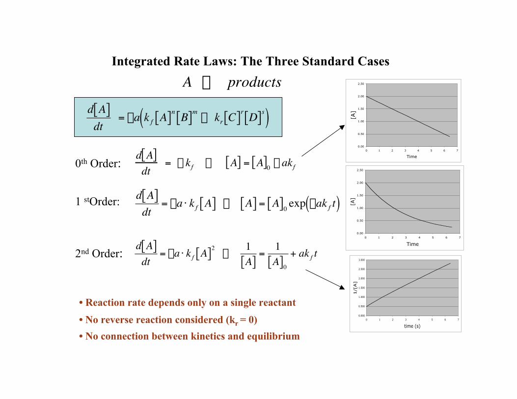
Integrated Rate Laws: The Three Standard Cases

• Reaction rate depends only on a single reactant

• No reverse reaction considered (kr = 0)

• No connection between kinetics and equilibrium

0th Order:

†

d A[ ]dt

= - kf fi A[ ] = A[ ]0 - akf

1 stOrder:

†

d A[ ]dt

= -a ⋅ k f A[ ] fi A[ ] = A[ ]0 exp -ak f t( )

2nd Order:

†

d A[ ]dt

= -a ⋅ k f A[ ]2 fi 1A[ ]

=1A[ ]0

+ ak f t

0.00

0.50

1.00

1.50

2.00

2.50

0 1 2 3 4 5 6 7

Time

[A]

0.00

0.50

1.00

1.50

2.00

2.50

0 1 2 3 4 5 6 7

Time

[A]

0.000

0.500

1.000

1.500

2.000

2.500

3.000

0 1 2 3 4 5 6 7

time (s)

1/[

A]

†

A Æ products

†

d A[ ]dt

= -a k f A[ ]n B[ ]m- kr C[ ]r D[ ]s( )

†

d A[ ]dt

= - a ⋅ Rnet A[ ] , B[ ] , C[ ] , D[ ]( )Consider the rate equation:

†

A[ ] i+1 @ [A]i - a ⋅ RnetDt

†

Dt = ti +1 - ti

†

A[ ]i+1 - [A]i

ti+1 - ti

@ - a ⋅ Rnet,i A[ ]i, B[ ]i, C[ ]i, D[ ]i( )

Euler’s Method uses successive linear approximations of a rate equation over short timeintervals to numerically integrate it over an arbitrarily long time interval.

†

A[ ] i+1is approximated concentrationat time

†

ti+1

†

[A]i is concentration at time

†

ti

Euler’s Method

t

[A]

Approximation error

†

A[ ]i+1

†

A[ ]i

†

ti+1

†

ti

Tangent line slope =

†

Rnet

Exact [A]

Comparison of Exact Solution to Euler’s Approximation for Simple First Order Rate Law

†

d A[ ]dt

= -a ⋅ k f A[ ] fi exact fi A[ ] = A[ ]0 exp -ak f t( )

†

Dt = 0.05s 40 intervals4 intervals

†

Dt = 0.5s

0.00

0.50

1.00

1.50

2.00

2.50

0 0.5 1 1.5 2 2.5

time (s)

[A]

[A], Euler

[A], exact

0.00

0.50

1.00

1.50

2.00

2.50

0 0.5 1 1.5 2 2.5

time (s)

[A]

[A], Euler

[A], exact

†

k f = 0.9 s-1

†

a =1

†

A[ ]0 = 2.0M

Outline of Spread Sheet Algorithm for Euler’s Method*

* Only [A] and [C] calculations explicitly shown

time

†

[A]

†

[B]

†

[C]

†

[D]

†

Rnet

†

Q

†

t0

†

[A]0

†

[B]0

†

[C]0

†

[D]0

†

Rnet ,0 = - k f A[ ]0n B[ ]0

m + kr C[ ]0r D[ ]0

s

†

C[ ]0c D[ ]0

d

A[ ]0a B[ ]0

b

†

t1 = t0 + Dt

†

A[ ]1 = A[ ]0 - a ⋅ Rnet ,0Dt

†

[B]1

†

C[ ]1 = C[ ]0 + c ⋅ Rnet ,0Dt

†

[D]1

†

Rnet ,1 = - k f A[ ]1n B[ ]1

m + kr C[ ]1r D[ ]1

s

†

C[ ]1c D[ ]1

d

A[ ]1a B[ ]1

b

†

t2 = t1 + Dt

†

A[ ]2 = A[ ]1 - a ⋅ Rnet ,1Dt

†

[B]2

†

C[ ]2 = C[ ]1 + c ⋅ Rnet ,1Dt

†

[D]2

†

Rnet ,2 = - k f A[ ]2n B[ ]2

m + kr C[ ]2r D[ ]2

s

†

C[ ]2c D[ ]2

d

A[ ]2a B[ ]2

b

†

t3 = t2 + Dt

†

A[ ]3 = A[ ]2 - a ⋅ Rnet ,2Dt

†

[B]3

†

C[ ]3 = C[ ]2 + c ⋅ Rnet ,2Dt

†

[D]3 etc.

to= 0 t [A] [B] [C] [D] Rnet Q∆t = 0.25 0 4.00 3.000 1 0.01 1.302 8E-04

0.25 3.674 2.6745 1.326 0.336 1.06 0.045[A]o= 4 0.5 3.409 2.4094 1.591 0.601 0.878 0.116[B]o= 3 0.75 3.19 2.1897 1.81 0.82 0.738 0.213[C]o= 1 1 3.005 2.0053 1.995 1.005 0.627 0.333[D]o= 0.01 1.25 2.849 1.8486 2.151 1.161 0.537 0.474

1.5 2.714 1.7143 2.286 1.296 0.465 0.636a= 1 1.75 2.598 1.5981 2.402 1.412 0.404 0.817b= 1 2 2.497 1.4971 2.503 1.513 0.354 1.013c= 1 2.25 2.409 1.4085 2.591 1.601 0.312 1.223d= 1 2.5 2.331 1.3307 2.669 1.679 0.275 1.445

2.75 2.262 1.2618 2.738 1.748 0.244 1.677m= 1 3 2.201 1.2007 2.799 1.809 0.218 1.917n= 1 3.25 2.146 1.1463 2.854 1.864 0.194 2.162r= 1 3.5 2.098 1.0977 2.902 1.912 0.174 2.41s= 1 3.75 2.054 1.0541 2.946 1.956 0.156 2.661

4 2.015 1.015 2.985 1.995 0.141 2.911T= 580 4.25 1.98 0.9799 3.02 2.03 0.127 3.161

4.5 1.948 0.9481 3.052 2.062 0.115 3.407∆H= -10000 4.75 1.919 0.9195 3.081 2.091 0.104 3.649

5 1.894 0.8936 3.106 2.116 0.094 3.886Ea,f = 160000 5.25 1.87 0.8701 3.13 2.14 0.085 4.116

5.5 1.849 0.8488 3.151 2.161 0.077 4.34Af= 2.79E+13 5.75 1.829 0.8294 3.171 2.181 0.07 4.556Ar= 2.79E+13 6 1.812 0.8118 3.188 2.198 0.064 4.764

6.25 1.796 0.7958 3.204 2.214 0.058 4.964kf= 0.108525 6.5 1.781 0.7813 3.219 2.229 0.053 5.155kr= 0.013643 6.75 1.768 0.768 3.232 2.242 0.048 5.337

7 1.756 0.7558 3.244 2.254 0.044 5.51

24.8 1.624 0.6241 3.376 2.386 1E-04 7.94725 1.624 0.624 3.376 2.386 1E-04 7.948

25.3 1.624 0.624 3.376 2.386 9E-05 7.94825.5 1.624 0.624 3.376 2.386 8E-05 7.949

Reagent Concentrations vs. Time

0.00

0.50

1.00

1.50

2.00

2.50

3.00

3.50

4.00

4.50

0 5 10 15 20 25 30

Time (s)

Conce

ntr

atio

n (

M)

[A] [B][C] [D]

Reaction Quotient vs Time

0

1

2

3

4

5

6

7

8

9

0 5 10 15 20 25 30

Time (s)

Q

Sample Spreadsheet and Graphs

A B C D E F G H I

1234567891011121314151617181920212223242526272829

[A] vs. Time

0.00

0.50

1.00

1.50

2.00

2.50

0 1 2 3 4 5

Time (s)

[A]

Reaction Rate vs. Time

0

0.5

1

1.5

2

2.5

3

0 1 2 3 4 5

Time (s)

React

ion

Rate

(M

/se

c)

†

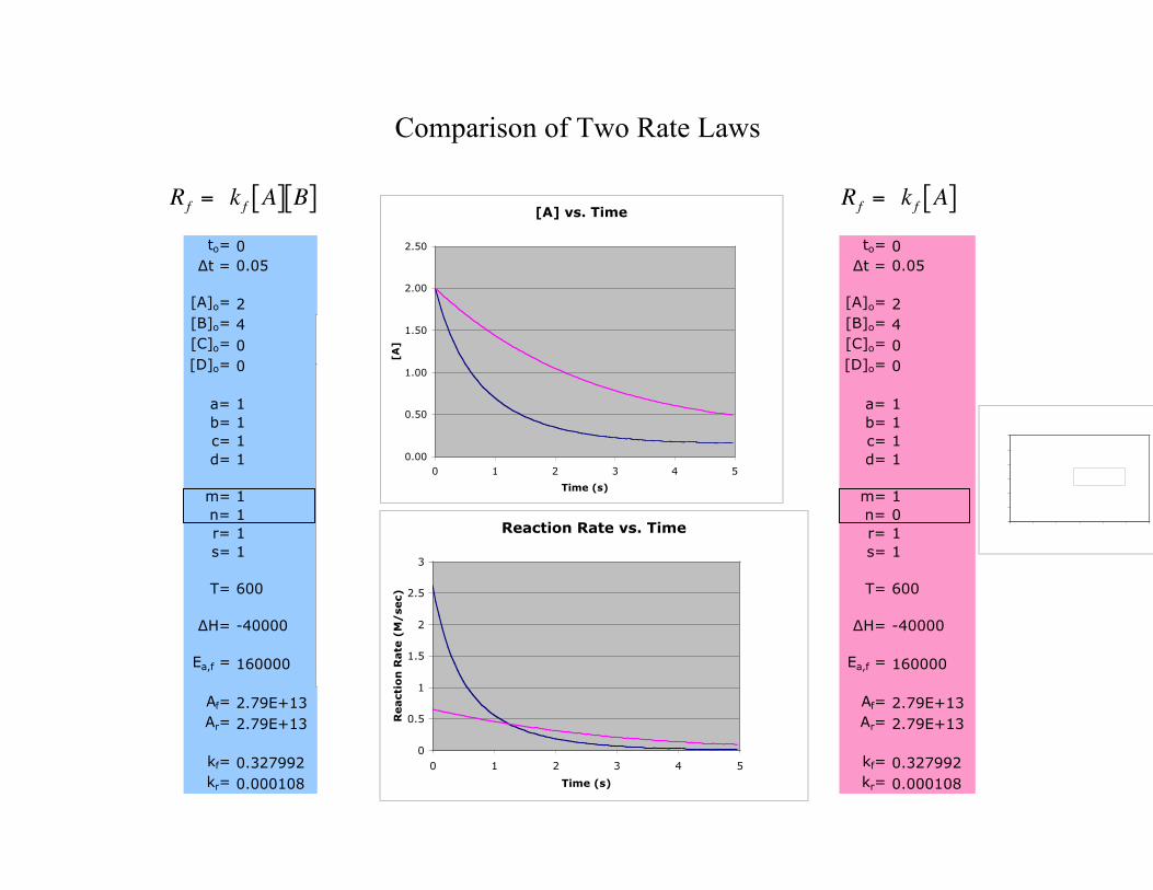
Rf = k f A[ ] B[ ]

†

Rf = k f A[ ]

Comparison of Two Rate Laws

to= 0∆t = 0.05

[A]o= 2[B]o= 4[C]o= 0[D]o= 0

a= 1b= 1c= 1d= 1

m= 1n= 1r= 1s= 1

T= 600

∆H= -40000

Ea,f = 160000

Af= 2.79E+13Ar= 2.79E+13

kf= 0.327992kr= 0.000108

[A] vs. Time

0.00

0.50

1.00

1.50

2.00

2.50

0 1 2 3 4 5

Time (s)

[A]

[A], M[A], M

Reaction Rate vs. Time

0

0.5

1

1.5

2

2.5

3

0 1 2 3 4 5

Time (s)

React

ion

Rate

(M

/se

c)

to= 0∆t = 0.05

[A]o= 2[B]o= 4[C]o= 0[D]o= 0

a= 1b= 1c= 1d= 1

m= 1n= 0r= 1s= 1

T= 600

∆H= -40000

Ea,f = 160000

Af= 2.79E+13Ar= 2.79E+13

kf= 0.327992kr= 0.000108

Reaction Quotient vs Time

0

10

20

30

40

50

60

0 1 2 3 4 5 6

time (s)

Q

Q (600 K)

Q (600 K)

Reaction Quotient vs Time

0

1

2

3

4

5

6

7

8

9

0 10 20 30 40 50

time (s)

Q

Reagent Concentrations vs. Time

0.00

0.50

1.00

1.50

2.00

2.50

3.00

3.50

4.00

4.50

0 10 20 30 40 50

Time (s)

Co

nce

ntr

ati

on

(M

)

[A] [B][C] [D]

Le Chatelier’s Principle: Concentration Stresses

• New equilibrium concentrations of reactants and products shifted

• Reaction quotient returns to the same equilibrium value as long astemperature remains constant.

Reaction Quotient vs Time

0

1

2

3

4

5

6

7

8

0 2 4 6 8 10

time (s)

Q Q (600 K)Q (610 K)

Le Chatelier’s Principle: Temperature Stress

• Temperature increase shifts equilibrium of exothermicreactions to the left (lowers the Keq).

• Reaction rate approximately doubles for every 10 Kincrease in temperature

to= 0∆t = 0.1

[A]o= 4[B]o= 3[C]o= 2[D]o= 1

a= 1b= 1c= 1d= 1

m= 1n= 1r= 1s= 1

T= 610

∆H= -10000

Ea,f = 160000

Af= 2.79E+13Ar= 2.79E+13

kf= 0.554907kr= 0.077247

to= 0∆t = 0.1

[A]o= 4[B]o= 3[C]o= 2[D]o= 1

a= 1b= 1c= 1d= 1

m= 1n= 1r= 1s= 1

T= 600

∆H= -10000

Ea,f = 160000

Af= 2.79E+13Ar= 2.79E+13

kf= 0.327992kr= 0.044183

Reaction Quotient vs Time

0

1

2

3

4

5

6

7

8

0 2 4 6 8 10 12

time (s)

Q Q (600 K)Q (610 K)

Effect of Catalyst (Lowering of Activation Energy)

Reaction Quotient vs Time

0

1

2

3

4

5

6

7

8

0 2 4 6 8 10

time (s)

Q Q (Ea,high)Q (Ea,low)

Lowering the activation energy increases reaction rate but doesnot alter equilibrium constant.

to= 0∆t = 0.08

[A]o= 4[B]o= 3[C]o= 2[D]o= 1

a= 1b= 1c= 1d= 1

m= 1n= 1r= 1s= 1

T= 600

∆H= -10000

Ea,f = 157000

Af= 2.79E+13Ar= 2.79E+13

kf= 0.598476kr= 0.080619

to= 0∆t = 0.1

[A]o= 4[B]o= 3[C]o= 2[D]o= 1

a= 1b= 1c= 1d= 1

m= 1n= 1r= 1s= 1

T= 600

∆H= -10000

Ea,f = 160000

Af= 2.79E+13Ar= 2.79E+13

kf= 0.327992kr= 0.044183

Reaction Quotient vs Time

0

1

2

3

4

5

6

7

8

0 2 4 6 8 10 12

time (s)

Q Q (600 K)Q (610 K)

†

NO(g) + O3(g) Æ NO2(g) + O2(g)

†

A =1.204 ¥109 Lmol ⋅ s†

DH = -1.99x105 Jmol

†

k f =10.836x106†

EA =11.7x103†

T = 298 K

From CRC Handbook

Depletion of ozone by nitric oxide in the upper atmosphere proceeds by the reaction

to= 0∆t = 0.0005

[A]o= 0.000021[B]o= 0.00002[C]o= 0.000001[D]o= 0

a= 1b= 1c= 1d= 1

m= 1n= 1r= 1s= 1

T= 298

∆H= -199000

Ea,f = 11700

Af= 1.20E+09Ar= 1.20E+09

kf= 10672940kr= 1.4E-28

Reagent Concentration vs. Time

0.00

0.00

0.00

0.00

0.00

0.00

0 0.005 0.01 0.015 0.02 0.025 0.03 0.035

time (s)

Conce

ntr

atio

n (

M)

[NO]

[O3]

[NO2]

[O2]

Suggestions for Use

• As a supplement to a teacher’s class presentation.

• As a basis for guided student explorations and problem sets.

• As a tool for analyzing experimental data.

Final Comments

• Integrating rate laws (solving differential equations) is fundamental to mathematicalmodeling in science. It is not necessary that students complete advanced courses incalculus before engaging in these calculations and benefiting from the insights andunifying understandings that follow.

• Most differential equations that describe real processes cannot be solved analytically.Yet, most readily yield to numerical methods requiring only basic algebra andarithmetic. The quantitative treatment of dynamic processes need not be limited tospecial cases. The “real world” can be more readily explored.

• Numerical integration methods transfer directly to topics in physics (and visa versa).

• Introducing students to spreadsheets is generally valuable.