the occurrence and distribution of mercury and co …
TRANSCRIPT

THE OCCURRENCE AND DISTRIBUTION OF MERCURY AND CO-OCCURING
METALS IN SELECTED NAMIBIAN AREAS AFFECTED BY INDUSTRIAL AND
MINING ACTIVITIES
A THESIS SUBMITTED IN FULFILMENT
OF THE REQUIREMENTS FOR THE DEGREE OF
MASTER OF SCIENCE CHEMISTRY
OF
THE UNIVERSITY OF NAMIBIA
BY
MARY MULELA MUTWA
200511131
MAIN SUPERVISOR: DR JULIEN LUSILAO (DEPARTMENT OF NATURAL AND
APPLIED SCIENCES, NUST)
CO-SUPERVISOR(S): PROF BENJAMIN MAPANI (DEPARTMENT OF
GEOLOGY, UNAM)
PROF VEIKKO UAHENGO (DEPARTMENT OF
CHEMISTRY AND BIOCHEMISTRY, UNAM)
i
Abstract
The occurrence and distribution of mercury (Hg) and other co-occurring heavy metals in
the mining towns of Berg Aukas and Tsumeb in northern Namibia were studied Different
forms of Hg and other heavy metals were characterized in soils, water and plants collected
in these areas. Total metal concentration was determined using ICP–OES and total Hg
was determined using the DMA 80 mercury analyser. Fractionation of Hg and other heavy
metals were determined by performing a four step sequential extraction procedure that
separates metals into four fractions, namely: exchangeable (F1), reducible (F2),
oxidisable (F3) and residual ( F4). Total metal results showed that there are high levels
of heavy metals in tailings from Berg Aukas in comparison to international guidelines
with, for example, Hg and Pb having concentrations as high as 2.24 mg/kg and 18 195
mg/kg, respectively. Although Berg Aukas soils generally showed Hg values beyond
guidelines threshold levels ( which is 1.0 mg/kg), the highest Hg concentration in soil
(3.49 mg/kg) was found at Tsumeb. Total metal concentration in water samples from
Berg Aukas showed Hg values higher than the maximum allowed for drinking water (up
to 6 µg/L). Some plants collected at Berg Aukas also had high Hg levels reaching a
maximum of 0.70 mg/kg in a sample collected from a pond. Distribution of Hg in tailings
found at Berg Aukas revealed that about 90% of Hg was residual whereas the
exchangeable (i.e. bioavailable) fraction accounts for about 7%. In contrast, the
exchangeable Hg fraction in Berg Aukas soils was as high as 35% of the total Hg. This
fraction may explain the presence of Hg measured in the surrounding plants and is a
reason for concern due to the risks of Hg methylation as well as further uptake of the
soluble forms of Hg by other living organisms. Other metals were also present in
bioavailable fractions and correlation analysis enabled the identification of several metal
compounds that were likely present in the study soils and tailings. Tailings are known to
be highly contaminated with heavy metals and this study demonstrates that these metals
are being dispersed into the surrounding soils that are used for agricultural purposes.
Keywords: Heavy metals, Sequential extraction, Hg, distribution, Tailings, soil, Berg
Aukas, Tsumeb

ii
Table of contents
Abstract ......................................................................................................................................... i
List of tables ................................................................................................................................. v
List of figures .............................................................................................................................. vi
List of abbreviations/acronyms ............................................................................................... viii
Acknowledgements ..................................................................................................................... xi
Dedication .................................................................................................................................. xii
Declaration .................................................................................................................................xiii
Chapter 1 ...................................................................................................................................... 1
Introduction ................................................................................................................................. 1
1.1 Background of study ......................................................................................................... 1
1.2 Statement of the Problem ................................................................................................. 7
1.3 Objectives of the study ...................................................................................................... 8
1.4 Significance of the study ................................................................................................... 9
1.5 Limitation of the study ...................................................................................................... 9
1.6 Delimitation of the study ................................................................................................... 9
Chapter 2 .................................................................................................................................... 10
Literature review ....................................................................................................................... 10
2.1 Mercury speciation .......................................................................................................... 11
2.1.1 Methylmercury ......................................................................................................... 13
2.2 Sequential extraction ....................................................................................................... 14
2.2.1 BCR extraction ......................................................................................................... 17
2.3 Study sites......................................................................................................................... 19
Chapter 3 .................................................................................................................................... 24
Research Methods ..................................................................................................................... 24
3.1 Research design ............................................................................................................... 24
3.2 Sampling ........................................................................................................................... 24
3.2.1 Tailings ...................................................................................................................... 24
3.2.2 Soil ............................................................................................................................. 26
3.2.3 Water ......................................................................................................................... 28

iii
3.2.4 Plants ......................................................................................................................... 29
3.3 Sample preparation for total metal analysis ................................................................. 31
3.3.1 Soil and tailing .......................................................................................................... 31
3.3.2 Plant sample preparation ........................................................................................ 33
3.3.3 The characterization of Hg and other metals distribution in affected study sites ..
............................................................................................................................. 33
3.3.4 Leaching procedure for sulphur and anions determination ................................. 35
3.4 Analytical techniques ...................................................................................................... 36
3.4.1 Mercury analysis of soil, tailings, plant and water ................................................ 36
3.4.2 Elemental analysis of soil, slag tailings, plant and water samples ....................... 37
3.4.3 Determination of anions ........................................................................................... 39
3.5 Data analysis .................................................................................................................... 40
3.6 Research Ethics ............................................................................................................... 40
Chapter 4 .................................................................................................................................... 41
Results ........................................................................................................................................ 41
4.1 Method validation ........................................................................................................... 41
4.1.1 Total elements ........................................................................................................... 41
4.1.2 BCR sequential extraction ....................................................................................... 42
4.2 Ancillary data for tailings, soils and waters .................................................................. 44
4.3 Occurrence of total mercury (HgT) in tailings, soils and plants ................................. 46
4.4 Occurrence of other heavy metals in Berg Aukas and Tsumeb .................................. 51
4.4.1 Tailings ...................................................................................................................... 51
4.4.2 Soil ............................................................................................................................. 53
4.4.3 Plants ......................................................................................................................... 54
4.4.4 Water ......................................................................................................................... 57
4.5 Fractionation of mercury in tailings and soils .............................................................. 58
4.5.1 Mercury fractions in tailings materials .................................................................. 58
4.5.2 Hg fractions in soils .................................................................................................. 59
4.6 Fractionation of co-occurring metals ............................................................................ 60
4.6.1 Arsenic (As) ............................................................................................................... 60
4.6.2 Cobalt (Co) ................................................................................................................ 61
4.6.3 Cadmium (Cd) .......................................................................................................... 63
4.6.4 Copper (Cu) .............................................................................................................. 65
iv
4.6.5 Lead (Pb) ................................................................................................................... 67
4.6.6 Manganese (Mn) ....................................................................................................... 69
4.6.8 Zinc (Zn) .................................................................................................................... 72
4.7 Occurrence of sulphur and anions in soils and tailings materials .............................. 74
Chapter 5 .................................................................................................................................... 79
Discussion ................................................................................................................................... 79
5.1 Occurrence of total mercury .......................................................................................... 79
5.2 Heavy metal concentrations ........................................................................................... 86
5.2.1 Soils and tailings ....................................................................................................... 86
5.2.2 Plants ......................................................................................................................... 94
5.3 Distribution and fractionation of mercury.................................................................... 96
5.4 Distribution and fractionation of co-occurring metals .............................................. 102
5.4.1 Arsenic (As) ............................................................................................................. 104
5.4.2 Cobalt (Co) .............................................................................................................. 105
5.4.3 Cadmium (Cd) ........................................................................................................ 105
5.4.4 Copper (Cu) ............................................................................................................ 108
5.4.5 Lead (Pb) ................................................................................................................. 109
5.4.7 Nickel (Ni) and chromium (Cr) ............................................................................. 111
5.4.8 Zinc (Zn) .................................................................................................................. 112
Chapter 6 .................................................................................................................................. 114
Conclusions and recommendations ....................................................................................... 114
6.1 Conclusions .................................................................................................................... 114
6.2 Recommendations ......................................................................................................... 118
References ................................................................................................................................ 119
Appendices ............................................................................................................................... 137
Appendix 1: Ethical Clearance Certificate ....................................................................... 137
Appendix 2: Tables 1-18 ..................................................................................................... 138

v
List of tables
Table 2.1: The BCR three-step sequential extraction ..................................................... 17 Table 2.2: Heavy metal composition of tailings and slags at Berg Aukas (2005-2007)
Mapani et al [33] ..................................................................................................... 21 Table 3.1: Description of tailing samples collected at Berg Aukas ............................... 26 Table 3.2: Description of soil, sediment and slag samples collected at Berg Aukas ..... 27
Table 3.3: Description of soil samples collected at Tsumeb .......................................... 27 Table 3.4: Description of water samples collected at Berg Aukas ................................. 29 Table 3.5: Microwave digestion parameters .................................................................. 32 Table 3.6: IC parameters for the analysis of anions ....................................................... 40 Table 4.1: Elemental concentrations of the CRM used for the validation of soils and
tailings analysis ....................................................................................................... 41
Table 4.2: Elemental concentrations of the CRM used for the validation of plant
analysis .................................................................................................................... 42
Table 4.3: Quality control of sequential extraction data using the CRM BCR-701
(n=3,RSD) ............................................................................................................... 43 Table 4.4: pH, EC and TDS of Berg Aukas tailings ...................................................... 44
Table 4.5: pH, EC and TDS values of soil from Berg Aukas (S1 to SL2) and Tsumeb
(S6 to S16) ............................................................................................................... 45 Table 4.6: pH, ORP and EC of Berg Aukas waters ........................................................ 46
Table 4.7: HgT in different parts of plants ..................................................................... 50 Table 4.8: Metals and metalloid in soils from Berg Aukas and Tsumeb ....................... 54
Table 4.9: Metals concentration (mg/kg) in leaf samples from Berg Aukas and Tsumeb
................................................................................................................................. 55
Table 4.10: Metal concentrations (mg/L) in Berg Aukas waters ................................... 58 Table 4.11: Anions in soil and tailings ........................................................................... 77
Table 5.1: Transfer coefficients of mercury for selected plants in Berg Aukas ............. 86 Table 5.2: Canadian soil quality guidelines for protection of environmental and human
health (mg/kg) [86] ................................................................................................. 87
Table 5.3: Concentrations (±SD) of trace metals from Oshakati, Northern Namibia,
unpolluted soils and other published mean sediments/soils values (in mg/kg) ...... 88 Table 5.4: EF categories [90] ......................................................................................... 90 Table 5.5: Enrichment Factors of selected heavy metals in Berg Aukas and Tsumeb
soils ......................................................................................................................... 91 Table 5.6: Correlation (Pearson correlation coefficients at P < 0.05) matrix between
metal concentrations in Berg Aukas and Tsumeb soils .......................................... 92 Table 5.7: Correlation matrix between metal concentrations, total sulphur and anions in
Berg Aukas tailings ................................................................................................. 93 Table 5.8: Correlation data between Hg fractions and other physico-chemical
parameters ............................................................................................................... 99 Table 5.9: Correlation data between Hg and physico-chemical parameters in Berg
Aukas tailings ........................................................................................................ 101
Table 5.10: Correlation analysis of data from Berg Aukas tailings ............................. 103
vi
List of figures
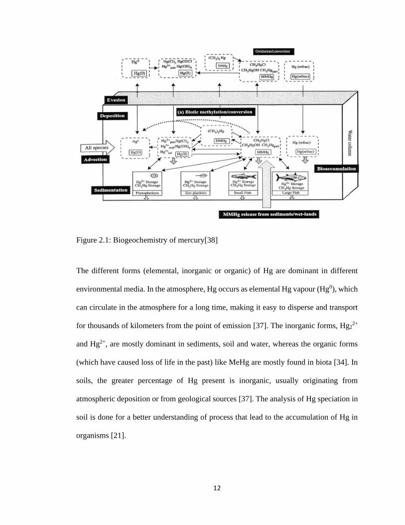
Figure 2.1: Biogeochemistry of mercury[38] ................................................................. 12
Figure 2.2: Berg Aukas map (Mapani et al [33]) ........................................................... 20 Figure 2.3: A map of Tsumeb (Dundee Precious Metal, 2019) ..................................... 23 Figure 3.1: Mine tailings at Berg Aukas ........................................................................ 25 Figure 3.2: A soil sampling area in Tsumeb ................................................................... 28 Figure 3.3: In situ measurement of ancillary data. ......................................................... 29
Figure 3.4: Some of the plant species that were collected. (a) Ricinus communis and (b)
Combretum imberbe ................................................................................................ 30 Figure 3.5: The sampling site at Berg Aukas (the blue dots are the sampling points) ... 30 Figure 3.6: The Tsumeb sampling site and sampling points (in green dots) .................. 31
Figure 3.7: The DMA-80 milestone instrument used for total Hg quantification .......... 36 Figure 3.8: Nickel boats with samples on the DMA 80 instrument ............................... 37
Figure 3.9: Inductively Coupled Plasma Optical Emission Spectrophotometer, ICPOES
(Optima 8000, Perkin Elmer) .................................................................................. 39 Figure 4.1: Calibration curves of low range (a) and high range (b) Hg of DMA 80...... 47
Figure 4.2: HgT in Berg Aukas tailings ......................................................................... 48 Figure 4.3: HgT in Berg Aukas and Tsumeb soils ......................................................... 49
Figure 4.4: HgT in plants (only results for leaves analysis are shown) ......................... 49 Figure 4.5: HgT in Berg Aukas waters ........................................................................... 51 Figure 4.6: Metals and metalloids in Berg Aukas tailings ............................................. 52
Figure 4.7: Metal concentrations in samples of different plant parts ............................. 57 Figure 4.8: Speciation of Hg in Berg Aukas tailings, (a)T sampling site and (b)TT
sampling site ............................................................................................................ 59
Figure 4.9: Speciation of Hg in soil samples from Berg Aukas and Tsumeb ................ 60
Figure 4.10: Speciation of As in Berg Aukas soils and tailings ..................................... 61 Figure 4.11: Speciation of Co in Berg Aukas and Tsumeb soils .................................... 62
Figure 4.12: Speciation of Co in Berg Aukas tailings .................................................... 63 Figure 4.13: Speciation of Cd in Berg Aukas and Tsumeb soils .................................... 64 Figure 4.14: Speciation of Cd in Berg Aukas tailings .................................................... 65
Figure 4.15: Speciation of Cu in Berg Aukas and Tsumeb soils .................................... 66 Figure 4.16: Speciation of Cu in Berg Aukas tailings .................................................... 67
Figure 4.17: Speciation of Pb in Berg Aukas and Tsumeb soils .................................... 68 Figure 4.18: Speciation of Pb in Berg Aukas tailings .................................................... 69 Figure 4.19: Speciation of Mn in soils from Berg Aukas and Tsumeb .......................... 70 Figure 4.20: Speciation of Mn in tailings from Berg Aukas .......................................... 71
Figure 4.21: Speciation of Ni in soils Berg Aukas and Tsumeb .................................... 72 Figure 4.22: Speciation of Zn in Berg Aukas and Tsumeb soils .................................... 73 Figure 4.23: Speciation of Zn in Berg Aukas tailings .................................................... 74
Figure 4.24: IC chromatogram of a multi-anion standard and calibration lines for
chloride and sulphate standards .............................................................................. 75 Figure 4.25: Total sulphur in soils, slags and tailings .................................................... 76 Figure 4.26: Sulphate versus sulphide in soils and tailings from Berg Aukas and
Tsumeb .................................................................................................................... 78

vii
Figure 5.1: Distribution of HgT in surface soils ............................................................. 80
Figure 5.2: Eh-pH diagram of Berg Aukas waters (The red arrows show the exact points
of the Eh-pH values for the corresponding samples) .............................................. 83 Figure 5.3: Eh-pH diagram showing Cd speciation in water [119] .............................. 107

viii
List of abbreviations/acronyms
AAS Atomic absorption spectrometry
AMAP Arctic monitoring and assessment programme
ANOVA Analysis of variance
BCR Community Bureau of Reference
CEC Cation exchange capacity
CPGS Centre of Postgraduate Studies
CRMs Certified reference materials
DMA Direct mercury analyser
DGM Dissolved gaseous mercury
EC Electrical conductivity
EF Enrichment factor
EPA Environmental Protection Agency
HgT Total mercury
IHg Inorganic mercury
MeHg Methylmercury
IC Ion chromatography
ix
ICP-OES Inductively coupled plasma optical emission
spectrophotometer
MET Ministry of Environment and Tourism
MFMR Ministry of Fisheries and Marine Resources
MME Ministry of Mines and Energy
NUST Namibia University of Science and Technology
ORP Oxidation-reduction potential
PEL Probable effect level
QC Quality control
RE Reference element
RSD Relative standard deviation
SE Sequential extraction
SEP Sequential extraction procedures
SD Standard deviation
SOM Soil organic matter
SPSS Statistical Package for the Social Sciences
SSE Selective sequential extraction
TC Transfer coefficient
x
TDS Total dissolved solids
TEL Threshold effect level
TET Toxic effect threshold
UNEP United Nations Environmental Programme
UREC University of Namibia Research Ethics Committee
USEPA US Environmental Protection Agency
WHO World Health Organisation
WHOGV World Health Organisation Guideline Value
XRD X-ray diffraction

xi
Acknowledgements
First and foremost, I would like to thank God Almighty, without His mercy and grace,
this study would have not been possible. Praise be to Him.
Secondly, I would like to thank my supervisors Dr Julien Lusilao, Prof Benjamin
Mapani and Prof Veiko Uahengo for their immense support, constructive comments,
motivation as well as their time and dedication throughout the duration of this study.
Many thanks to Dr Roswitha Hamunyela for your presence during sampling. You
availed your car and time to Tsumeb and Berg Aukas and made this journey more fun.
To Simeon Ambuga, Ilenikuye Thomas, Peter Shabani, Nicholetta Kupembona and
Hilma Haufiku, your assistance in the laboratory was highly appreciated. Thank you and
May God bless you. To Mr. Erich Naoseb of the Geo-Spatial Sciences and Technology
department of the Namibia University of Science and Technology (NUST), your
assistance with the GIS mapping software was highly appreciated. Thank you once again
for your time and effort. Mr. Kayini Chigayo, thank you for always willing to assist
whenever I got stuck. I will forever be grateful.
Special thanks also go to Mr. Steven Hamutenya from the Ministry of Fisheries and
Marine Resources (MFMR), Swakopmund. You saved the day with your assistance with
the mercury analyser at the very last minute. I will forever be grateful. God bless you.
Gratitude also goes to my colleagues, friends and family. You believed in me. Your
continuous words of encouragement kept me going.
Lastly, to my daughter, Abbygail, you kept pushing me (in your own little special way).
Having you as a daughter motivates me in more ways than one. Thank you, my girl.

xii
Dedication
To my daughter Abbygail Asino, my sister Sara Mutwa and my father John Mutwa.

xiii
Declaration
I, Mary Mulela Mutwa, hereby declare that this study is my own work and is a true
reflection of my research, and that this work, or any part thereof has not been submitted
for a degree at any other institution.
No part of this thesis may be reproduced, stored in any retrieval system, or transmitted in
any form, or by means (e.g. electronic, mechanical, photocopying, recording or
otherwise) without the prior permission of the author, or The University of Namibia in
that behalf.
I, Mary Mulela Mutwa, grant the University of Namibia the right to reproduce this thesis
in whole or in part, in any manner or format, which The University of Namibia may deem
fit.
…………………. ……………… ……….…………
Name of Student Signature Date
1
Chapter 1
Introduction
1.1 Background of study
The last few decades have seen an increase in urbanization and industrialization, which
led to large amounts of toxic contaminants, such as heavy metals, being released into the
environment. Besides the fact that some of these contaminants occur naturally in the
environment as part of the earth’s crust, some anthropogenic sources, especially mining
activities, have contributed significantly to their increase [1]. Since some of these
contaminants are heavy metals which cannot be destroyed and are not degradable, they
persist and accumulate in the environment [2].
Heavy metal pollution is especially very prominent in areas of active and closed mining
sites. Heavy metals commonly found at contaminated sites are lead (Pb), chromium (Cr),
arsenic (As), zinc (Zn), cadmium (Cd), copper (Cu), mercury (Hg), cobalt (Co) and nickel
(Ni). These metals pose a chemical hazard to the environment and each of these metals
will result in different behavioural and physiological changes when an individual is
exposed to them [3]. Heavy metals are persistent environmental contaminants and occur
as natural constituents of the earth crust, and since they cannot be degraded or destroyed
[2]. Additionally, heavy metals, especially Cu, Ni, Cd, Zn, Cr and Pb, are considered to
be one of the major sources of soil pollution [1].
One of the most commonly studied heavy metals is mercury (Hg). Hg is one of the most
toxic and volatile elements [2]. It is a naturally occurring metal that is found as a liquid
at room temperature and exists in three different forms namely, elemental (Hg0),

2
inorganic (Hg22+ and Hg2+) and organic (RHgX) Hg species. All Hg species are highly
toxic when humans are exposed to them [4]. Even though Hg has no biological function
in humans, long term exposure (usually through ingestion of Hg containing food or
inhalation of mine waste particles with elevated Hg levels) is a potential health hazard
[5].
Hg is a widespread contaminant that affects humans and environmental health negatively
(mainly by contaminating soils, surface water, groundwater and air).This is mostly due
to its high toxicity, global transport, persistence and bioaccumulation in the environment
[6]. It is released into the environment by both natural processes and anthropogenic
activities. Moreover, Hg pollution is considered as a global problem because of its
volatility and persistency, once it is released into the environment, it can travel and settle
thousands of kilometers away from its original emission source. Even though the
emission is local or regional, it can cause air, soil and water pollution, which can be felt
globally [7]. The main sources of Hg pollution in the environment are fossil fuel burning,
especially coal; mining, high temperature combustion [8] and artisanal gold processing,
where Hg is used to form gold amalgam [9] that is used to scavenge fine gold particles.
Once released into waterways, Hg enters the food chain through digestion by bacteria and
is converted to methylmercury, a highly toxic form of Hg. Even though methylmercury
is the most toxic form, all Hg forms are toxic to the environment and human health [10].
Hg pollution due to anthropogenic activities is higher in the northern hemisphere (Figure
1.2) due to greater industrial activity and population density [11]. Over the years, mining
has been an ongoing source of Hg contamination to the environment [12]. Hg is released
into and enters the environment as a result of various anthropogenic activities, which

3
include fossil-fuel fired power plants, ferrous and non-ferrous metals manufacturing
facilities, cement plants, chemical production facilities and mining activities [13] (Figure
1.1). In addition, anthropogenic emissions continue to add significantly to the global pool
of Hg and due to the rise of industrial activities over the years, anthropogenic activities
have introduced substantial amounts of Hg into the environment at an alarming rate [14].
This contributes about 30% of the total emissions to the global atmosphere, whereas re-
emissions comprise about 60% of Hg emissions [15]. As shown in Figures 1.1 and 1.2,
mining, ore processing and high temperature processes such as coal burning, dominate
anthropogenic inputs of Hg to the atmosphere [11].
Figure 1.1: Global anthropogenic Hg emissions to air in 2010 [13]

4
Figure 1.2: Global distribution of Hg-contaminated sites [11]
Contamination of Hg to the environment and human health has deleterious effects,
especially if it occurs in highly toxic and soluble species such as mercuric chloride
(HgCl2) or methyl mercury (CH3HgX). Additionally, environmental Hg levels have been
on the rise since the beginning of industrialisation and have consistently progressed ever
since. Highly contaminated and abandoned industrial sites as well as active mining
operations continue to release Hg into the environment [16]. When released in the
environment, Hg usually ends up in the atmosphere, water and soil.
Contamination of soil by heavy metals can happen in various ways and is of great concern
to food production and human health. Soils may become contaminated with heavy metals
through emissions from industrial and mining activities, these include but are not limited
to mine tailings, disposal of metal wastes, spillage of chemicals and agricultural activities
such as the application of inorganic fertilisers [3]. These activities have led to a worldwide
contamination of soil by heavy metals such as Cu, Zn, Pb, Cd, Mn, Cr, As and Hg. In
5
addition, if the concentrations of heavy metals exceed the attenuation capacity of soil,
soil pollution will occur, even though soil has a natural capacity to attenuate heavy metals
through various mechanisms [4]. Some of these metals, especially Hg, are mobile and
readily bioavailable. Due to its bioavailability, Hg can be taken up by plants and other
living organisms, a process known as bioaccumulation, subsequently causing
biomagnification further up in the food chain [14]. Moreover, once Hg is deposited into
soil, it can be transformed into different species by different environmental soil conditions
such as pH, temperature, presence of microorganisms and humus content, which may
favour the formation of some organic and inorganic species of Hg, thus displaying
different mobility rates in the soil [17]. In comparison to other heavy metals, Hg is much
more persistent in soils [4].
One of the negative environmental impact caused by mining and other anthropogenic
activities is mining tailings, some of which can be toxic waste from mineral processing
of ore after the metals have been extracted. The impacts caused by mine tailings can go
on for years after mining activities have ceased [18], adversely affecting the surrounding
vegetation, leading to changes in species composition [19]. In dry areas, mine tailings
are important sources of soil pollution because highly contaminated particles can be
dispersed by water and wind, which aids in mobilising the tailings’ metal contents into
the environment [20]. This mobilisation could lead up to trace metal contamination of
surface soils. Therefore, contamination from mine tailings does not only affect the tailing
sites but can cover large land areas including agricultural soils, posing serious
environmental soil degradation. These problems continue to increase over the years [21].

6
The release of Hg from anthropogenic activities into aquatic systems is of huge concern
because Hg has a potential of being transformed from inorganic Hg to more toxic organic
forms [22]. Once Hg is in the waterways, even at low concentrations, it is methylated by
algae and bacteria. Methylmercury (MeHg) then bio-accumulates and biomagnifies to
unsafe levels in the food chain, into fish and eventually in humans. Hg is released into
water through industrial pollution from natural sources and anthropogenic activities as
well as through a natural process of off-gassing from the earth’s crust [23]. One of the
largest contributors to high levels of Hg in fresh water may be the direct release of Hg
into water [24].
Agriculture is one of the sectors that are crucial for human sustainability worldwide.
However, with the increase of industrial activities over the years, there is a risk of
continuous pollution of heavy metals to plants, which if consumed by humans or animals,
can have detrimental effects [25].
Hg is introduced to agricultural land through sludge, fertilizers, lime and manure. Once
this organic form of Hg is taken up by the plant, the Hg concentration will increase [26].
However, the amount of Hg that is taken up by the roots from the soil depends on factors
such as pH, type of soil, soil aeration, plant species and cation-exchange capacity [25]. In
addition to plants taking up Hg from water and soil via roots, plants are also able to absorb
Hg that is deposited on leaf surfaces. Accumulation of most of the Hg in plants is done
so with minimal mobility, meaning only a small percentage is released into the
atmosphere or is transported to other parts of the plant. Once accumulated in plants, Hg
can be found in different forms, namely Hg (0), Hg (II) and organic Hg, with aquatic
plants usually containing more methyl mercury (organic Hg) than terrestrial plants [27].

7
1.2 Statement of the Problem
Industrial activities such as mining generate waste that may contain high concentrations
of metals which can be mobilised. Most of the heavy metals are highly toxic and are not
biodegradable [28]. Unlike other pollutants like petroleum hydrocarbons and domestic
and municipal waste which may visibly build up in the environment, trace metals such as
Hg may accumulate in the environment to toxic levels unnoticed. In addition, Hg has
been directly mobilised by humans for thousands of years into aquatic and terrestrial
ecosystems through mining and metallurgical processes [29]. Unfortunately, there are
limited data concerning the extent of Hg pollution in the southern hemisphere, especially
on the African continent (Figure 1.2). For instance, the contribution of Hg pollution from
milling, smelting and refining of sulphide ores, which are known potential sources of
heavy metals, releases heavy metals into the environment, and thus cause pollution on
various scales. This pollution, especially from Hg, is not adequately quantified in the
Namibian context. There is, therefore, an urgent need of providing reliable data on the
occurrence and release of heavy metals such as Hg in local environmental compartments
affected by the above-mentioned mining activities to partly fill the currently existing gap
concerning Hg emission data on the continent.
A study conducted by Podolsky et al [20] in the central-northern region of Namibia and
Zambia found that there were high concentrations of total elemental Hg in soils from
mining/smelting in northern Namibia than in the Zambian Copperbelt. Another study
conducted by Kamona et al [30] in the southern region of Namibia reported high average
values of Hg and other metals in dust emanating from the crusher at the Rosh Pinah mine.
These metals were Zn, Pb, Cu, As, Hg, Cr and Cd. Furthermore, this study revealed that
8
there were high concentrations of total S as well as high values of As, Hg, Pb and Zn in
soils that are close to the tailing dams.
Some characteristics of Hg such as absorption, mobility, bioavailability and toxicity
depend on its chemical forms [31]. Though these studies reported total Hg concentration,
no information on Hg forms (i.e. speciation) was provided. Total elemental analysis is
not enough to provide such information; therefore Hg speciation is needed [32]. This
further highlights the necessity of speciation studies in the Namibian context to better
understand the distribution and ecosystem fate of Hg and co-occurring metals found in
areas impacted by mining activities.
1.3 Objectives of the study
a) To study the occurrence of Hg and other co-occurring metals in tailings, soils,
slags, plants and waters from local areas situated near abandoned and active
mining operations at Berg Aukas and Tsumeb.
b) To characterise the different forms (species) of Hg and other heavy metals
occurring in the affected study sites.
c) To compare these findings with those reported worldwide, especially in areas with
similar environmental and climatic conditions (i.e. semi-arid areas) and to infer
from these results the likely mechanism of Hg and co-occurring metals dispersal
in the study areas as well as the ecosystem risks associated with the occurrence of
the observed Hg species.
9
1.4 Significance of the study
Hg occurrence in Namibia was reported at the Tsumeb mine, in Berg Aukas, at the Rosh
Pinah Pb and Zn mine and at the Kombat mine. The highest Hg concentration was
observed in soil samples from Tsumeb [20] as well at the Rosh Pinah lead and zinc mine
in southern Namibia where the dust originating from the crusher was found to have Hg
levels of 1.05 mg/kg, a value that is of great environmental concern [30]. Hg release leads
to an increase in the amount of the metal in the atmosphere, where it enters the
atmospheric-soil-water distribution cycles and it can remain in circulation for years, thus
posing a high risk of Hg exposure, depending on the chemical form and route of exposure
[28]. Therefore, this study, through speciation data, provides relevant information for
toxicological studies and mitigation purposes, making it possible to develop the right
approach in eliminating or reducing the occurrence of Hg in the affected areas.
1.5 Limitation of the study
Permission to access some of the active and abandoned sites was a limitation to this study.
1.6 Delimitation of the study
The study focused on areas affected by industrial activities, where permission to access
the sites was given.

10
Chapter 2
Literature review
Heavy metal pollution has been a severe problem in many parts of the world, due to rapid
social and economic development over the past few decades. Even though trace amounts
of heavy metals like Cu, Zn, Co, Ng, Ni, and Fe are needed for growth of living
organisms, these heavy metals can be harmful when their concentrations go beyond the
permissible limits. Other heavy metals such as cadmium, lead and mercury do not have
any beneficial effects on living organisms [3]. In comparison to other heavy metals, Hg
has two unique properties: 1) it is highly soluble in water and 2) in its pure form, elemental
Hg, exists as liquid at room temperature, resulting in it slowly forming a vapour in the air
[25]. In addition, Hg is a unique metal because it occurs in the environment in three
different chemical forms that have different properties, usage and toxicity [33]. These
forms are elemental Hg, inorganic Hg and organic Hg. The inorganic and organic Hg are
more commonly Hg forms found in nature [34]. These forms enter human bodies in
distinct ways, including, but not limited to, eating fish or wild game near the top of the
food-chain that have high levels of Hg in their tissues and playing on or in contaminated
surfaces and soils [35]. Exposure from polluted air and drinking water is usually minor.
Of these forms, methylmercury is the most dangerous [36]. Properties of Hg and
behaviour (e.g. bioavailability, transport, toxicity, etc.) will mostly depend on the
chemical forms of occurrence (speciation), rather than on its concentration level in a given
environmental compartment [34]. Thus, characterizing the Hg distribution (i.e. its
speciation) provides important data when predicting metal bioavailability that appears to
11
be site, media and matrix specific and will be of relevance, not only within the context of
application to health risk assessments but also for mitigation purposes [31].
2.1 Mercury speciation
Hg is a toxic and hazardous pollutant that occurs in the environment in three different
chemical forms that have different properties, usage and toxicity. The pure form,
elemental Hg, is liquid at room temperature and slowly forms a vapour in the air at about
70°C [37]. Of the organic forms, methylmercury is the most dangerous because it inhibits
many neurobiological processes in infants, children and adults [31]. Figure 2.1 shows
how the different species of Hg occur in sediments, water and air [38]. In aquatic
environments, the speciation of Hg is dependent on factors such as the pH of the water,
the pE and the composition of the water matrix. Additionally, once Hg is deposited in
natural waters, it undergoes an aquatic redox cycling between oxidized Hg (Hg2+),
dissolved gaseous Hg0 (DGM), and MeHg [34]. In aquatic food webs, the bio-
concentration of MeHg is the reason global health advisories caution against the
consumption of fish that might contain elevated levels of MeHg [39].
12
Figure 2.1: Biogeochemistry of mercury[38]
The different forms (elemental, inorganic or organic) of Hg are dominant in different
environmental media. In the atmosphere, Hg occurs as elemental Hg vapour (Hg0), which
can circulate in the atmosphere for a long time, making it easy to disperse and transport
for thousands of kilometers from the point of emission [37]. The inorganic forms, Hg22+
and Hg2+, are mostly dominant in sediments, soil and water, whereas the organic forms
(which have caused loss of life in the past) like MeHg are mostly found in biota [34]. In
soils, the greater percentage of Hg present is inorganic, usually originating from
atmospheric deposition or from geological sources [37]. The analysis of Hg speciation in
soil is done for a better understanding of process that lead to the accumulation of Hg in
organisms [21].

13
Speciation of Hg has not been studied in the Namibian context. However, a study on
contaminated soils in Switzerland was conducted and found that exchangeable Hg was
found in low amounts (1.5%) of the total mercury (HgT) [17]. Furthermore, the study
reported that most of the Hg was found in the oxidisable fraction [17]. Additionally, Hg
speciation was also studied in soils from Randfontein in South Africa [18]. In the
Randfontein study, the authors found that soils from Randfontein mostly had oxidisable
Hg, measuring up to a maximum of 52% [18].
2.1.1 Methylmercury
All forms of Hg are considered toxic but the organic forms such as MeHg are the most
toxic. This form of Hg is widely studied because it affects large populations, and its
toxicity is better characterised than that of other organic Hg compounds [29]. Inorganic
forms of Hg are potentially converted to MeHg once they enter aquatic environments,
usually by the action of microorganisms [40]. Due to its bioaccumulation and nature,
MeHg spreads to the food where animals at the top of the food chain are likely to
accumulate higher concentrations of MeHg, consequently getting MeHg poisoning
(Figure 2.1). The primary signs and symptoms of MeHg poisoning are loss of sensation
around the mouth, in the hands and feet, slurred speech, blindness or reduced vision and
loss of hearing [34].
Two MeHg poisonings occurred in Japan (in the city of Minamata) and in Iraq [39].
Minamata is a small coastal town in the southern parts of Japan and it has abundant fishing
resources. In 1956, Hg-containing waste was released in the industrial wastewater from
the Chisso Corporation's chemical factory, which produced fertilizers, acetylene,
acetaldehyde, acetic acid and vinyl chloride [39]. Moreover, the production of

14
acetaldehyde used mercury sulfate as a catalyst [39]. Once in water, Hg was converted to
MeHg by aquatic biota [34]. MeHg then bio-accumulated in fish and shellfish in
Minamata Bay and the Shiranui Sea, which when eaten by the local population, resulted
in MeHg poisoning [41].
In late 1971 and early 1972, the largest global outbreak of Hg poisoning occurred in Iraq
[42]. This poisoning involved the ingestion of homemade wheat bread, whose seed grain
was treated with MeHg fungicide to protect it from fungi infestation before planting [42].
MeHg is used in fungicides because it is known to have antifungal properties when
applied to seed grain [42]. Moreover, the seed was not meant for consumption but rather
for planting, but due to unforeseen circumstances, a farmer used it to make bread and fed
it to domestic animals and humans. After the first human developed severe symptoms of
Hg poisoning, the people were informed of the toxicity of the wheat [42]. This led to
many farmers disposing the wheat all over the country, with some of it reaching the
waterbodies, causing contamination of fish and birds and ultimately leading to an
environmental disaster [43].
2.2 Sequential extraction
The concentration of total metals in soil is usually used as a soil pollution indicator.
However, it is not enough in evaluating heavy metal contamination and does not provide
information about toxicity, distribution, chemical interactions, mobility and/or
bioavailability of metals [44].
Fractionation methods are amongst some of the many separation techniques that have
been widely applied over the years to characterise the environmental reactivity of

15
potentially toxic elements in liquid and solid phases [44]. For solid phases, sequential
extraction (SE) is one of the methods used to characterise different fractions comprising
of phases that are associated with potentially toxic elements [45]. Sequential extraction
is a technique whereby a series of chemical reagents are applied to a solid sample in
succession and elements are separated into specific fractions by selective extraction [44].
In addition, it provides information about the origin, mode of occurrence, bioavailability
and mobility of trace metals in solid samples, which depends on the composition of the
leaching solution, the characteristics of the solid, as well as the strength of the bond
between the heavy metal and the solid matrix [37].
All sequential extraction procedures are enabled by fractionation. These fractions are
named exchangeable, weakly absorbed, hydrous oxide bound, organic bound and lattice
material components [44]. In addition, sequential extraction procedures are based on the
theory that the most mobile metals are removed in the first fraction. The removal of metals
continues in order of decreasing mobility [46].
Hg is one of the few elements that has an in-depth study of its form of occurrence
(speciation) or fractional products as well as distribution [47]. In addition, the
accumulation of trace metals such as Hg in soil is a serious environmental concern that
creates a hazard when metals are transferred to water or plants. Due to the mobility and
bioavailability of trace metals, there exists potential toxicity of trace metals in soil, thus
trace metals can cause detrimental damage to the nervous system when the water or plants
are consumed by humans and animals [48].
Although there exist several available sequential extraction methods developed over the
last three decades, the debate continues as to which technique is preferable over the others

16
[37]. This is largely because the wide variety of techniques developed and used makes
comparison of the different techniques difficult, a fact attributed to the optimisation of
sequential extraction processes for solids and trace metals [37].
The first sequential extraction method was a seven-step method developed by Tessier et
al. [49] who classified potentially toxic elements according to their solubility and binding
forms of metallic species. Due to the time demand of seven-step (7–10 days), a three-step
sequential extraction method known as the Community Bureau of Reference (BCR) was
introduced by the European Community Bureau of Reference[50]. This procedure is
largely similar to that produced by Tessier et al. [49], with the chief difference in the first
fraction of the procedure. Instead of evaluating the exchangeable and carbonate bound
separately, the BCR procedure combines both in the first fraction [50].
In Namibia, sequential extraction has been applied in several studies, using the BCR
procedure. One such study was conducted by Sracek et al [51] who looked at the
geochemistry and mineralogy of vanadium and iron in mine tailings at Berg Aukas. This
study found low solubility and water leached concentrations of V as well as low Fe
content. In addition, this study also looked at the formation of secondary hematite by
performing sequential extraction for Fe and As in Kombat and that most of the As found
in the mine tailings is residual. Moreover, sequential extraction was employed in another
study that looked at the agricultural soil contamination by potentially toxic metals (Cu
and Pb) dispersed from improperly disposed tailings at the Kombat mine [52]. This study
by Mileusnic et al [52] found that the dominant fraction of Pb in mine tailings is the
reducible fraction Pb, which constituted about 60% of the total Pb. This was followed by

17
the carbonate fraction with about 30% of the total Pb while the exchangeable and
oxidisable fraction had about 10 and 1%, respectively. The study further found that the
distribution of Cu in the tailings varied. The reducible fraction of Cu contained about 30-
60% of total Cu, oxidisable fraction about 10-40%, carbonates 10-20% and exchangeable
fraction about 20%.
2.2.1 BCR extraction
Over the years, the use of sequential extraction procedures has increased. This is because
these procedures may provide comparative information on mobility of trace metals in soil
with varying environmental conditions. The BCR is a stepwise sequential extraction
method that analyses different fractions of metals in soil. These fractions are acid
extractable, reducible, oxidisable and residual [48]. The three steps involved in the BCR
extraction [53] are shown in Table 2.1.
Table 2.1: The BCR three-step sequential extraction
Extraction
step
Reactive /concentration/ pH Solid phase/Fraction
1 Acetic acid (CH3COOH, 0.11 molL−1),
pH 2.85
Exchangeable, water and acid
soluble (e.g. carbonates)
2 Hydroxylammonium chloride
(NH2OH·HCl, 0.1 molL−1) , pH 2
Reducible (e.g.
iron/manganese oxides)
3 Hydrogen peroxide (H2O2, 8.8 molL−1),
followed by ammonium acetate
(CH3COONH4, 1.0 molL−1) , pH 2
Oxidisable (e.g. organic
substance and sulphides)

18
Residuala Aqua regia (3HCl + HNO3) Remaining, silicate bound
metals
aDigestion of the residual material is not a speciation of the BCR protocol.
This method aims at minimising errors during the treatment and analysis of samples. In
addition, it seeks to identify the most appropriate analytical procedure as well as to supply
reference materials for comparison of results. Moreover, this method appears to be, in
comparison to others proposed previously, such as that of Tessier et al [49], more
operationally effective [54].
When introduced in 1993 by the European Community Bureau of Reference, the BCR
was just a three-step method but it has since been modified by Rauret et al [50] where a
fourth step was added. Trace metals accumulate in soil, causing a serious environmental
problem that creates a hazard when metals are transferred to water or plants. In order to
understand the mobility and bioavailability of trace metals for different physicochemical
phases of the soil, the concentrations and distributions of trace metals must be established
[48].
There are three main ways that can be used to identify Hg species during fractionation
methodologies, namely: chemical, thermo-desorption and X-ray absorption techniques
[55]. However, applicability with the X-ray techniques in environmental samples is very
limited because these techniques are expensive and require samples with mercury
concentration greater than 100 mg/kg. In the few last decades, several researchers have
developed and published sequential extraction methods that are more specific to Hg [55].
While some of the methods evaluate Hg availability and can be applied to a wide range
of solid samples [56], other researchers proposed solutions that evaluate Hg mobility by
19
applying methods that determine limited number of fractions, like those associated with
sulfides [57].
Furthermore, selective extraction methods use extractants to release different fractions of
Hg and assess the amounts of mobile Hg. This information can be used to correlate the
plant-available contents under certain environmental or agricultural conditions. Even
though these methods are capable of quantifying Hg at low levels (< 0.005 mg/kg), they
are not suitable for Hg because of its diverse species [58].
Among the existing methods that are used for Hg fractionation in environmental samples,
a 5 step selective sequential extraction (SSE) developed by Bloom et al [56] and the EPA
method that is known as EPA method 3200 are procedures that can provide information
on the distribution of Hg and consequently help determine what remediation steps to take
[59].
2.3 Study sites
Berg Aukas, which is located at 19° 34' 12'' S, 18° 15' 36'' E, was a mining town
discovered in 1913, where they used to mine and roast ores of Pb, V and Zn until its
closure in 1979 [33]. In the early 90’s, the government of Namibia turned the abandoned
mine buildings located at the town of Berg Aukas into a National Youth Training centre,
where activities such as livestock farming, horticulture as well as seasonal crop farming
are taking place. This abandoned mine is known to be polluted with heavy metals such
Pb, Zn, Cu, Cd, As, Hg and Mo [60].
Due to the mine tailings located north of the mining area (as seen in Figure 2.1) that have
been left unattended since the closure of the mine and slag deposits that are centrally

20
located with an eroded sealing, these conditions presents a huge source of dust that is
dispersed across large distances. In addition, environmental factors such as wind and
rainfall have resulted in heavy metal contamination of areas that are further away from
the abandoned mining site [33]. These mine tailings are not fenced off, thus, posing a
health hazard to the local population.
Figure 2.2: Berg Aukas map (Mapani et al [33])
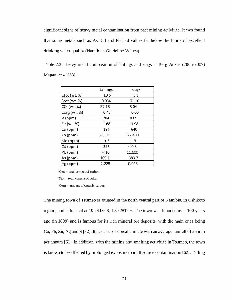
A study conducted by Mapani et al [33] between 2005 and 2007 that aimed at assessing
potential human health risks that might arise from consumption of crops and water in and
around Berg Aukas found that there were parts of the soil, tailings and vegetation (Table
2.2) in the Berg Aukas area that were severely contaminated with heavy metals, with Hg
being one of the heavy metals. In addition, this study showed that all water samples from
Berg Aukas were of excellent quality in terms of conductivity. Moreover, the study also
concluded that the groundwater in Berg Aukas and surrounding areas did not show any
21
significant signs of heavy metal contamination from past mining activities. It was found
that some metals such as As, Cd and Pb had values far below the limits of excellent
drinking water quality (Namibian Guideline Values).
Table 2.2: Heavy metal composition of tailings and slags at Berg Aukas (2005-2007)
Mapani et al [33]
*Ctot = total content of carbon
*Stot = total content of sulfur
*Corg = amount of organic carbon
The mining town of Tsumeb is situated in the north central part of Namibia, in Oshikoto
region, and is located at 19.2443° S, 17.7281° E. The town was founded over 100 years
ago (in 1899) and is famous for its rich mineral ore deposits, with the main ones being
Cu, Pb, Zn, Ag and S [32]. It has a sub-tropical climate with an average rainfall of 55 mm
per annum [61]. In addition, with the mining and smelting activities in Tsumeb, the town
is known to be affected by prolonged exposure to multisource contamination [62]. Tailing
Ctot (wt. %) 10.5 5.1
Stot (wt. %) 0.034 0.110
CO (wt. %) 37.16 6.04
Corg (wt. %) 0.42 0.00
V (ppm) 704 832
Fe (wt. %) 1.68 3.98
Cu (ppm) 184 640
Zn (ppm) 52,100 22,400
Mo (ppm) < 5 13
Cd (ppm) 352 < 0.8
Pb (ppm) < 10 11,600
As (ppm) 109.1 383.7
Hg (ppm) 2.228 0.028
tailings slags

22
dumps, slag deposits as well as solid and gaseous emissions from past and recent mining
activities are sources of heavy metal contamination in Tsumeb [63].
A study done in 2015 by Hange et al [14] on soils in Tsumeb showed elevated levels of
Cu, Zn, Pb and Cd at selected sampling points with concentrations of 39.0-2532.8 mg/kg,
59.5-1994.8 mg/kg, 1.2-141 mg/kg and 1.7-21.3 mg/kg respectively [14]. In addition, the
overall mean concentration of the selected metals was found to be higher than the
international threshold limits of 100 mg/kg for Cu, 200 mg/kg for Zn, 60 mg/kg for and
1 mg/kg for Cd. The study concluded that anthropogenic activities have an influence on
heavy metal levels in soil [14].
Furthermore, another study conducted by Podolsky et al [20] on mercury in soils in
Zambia and Namibia (Berg Aukas and Tsumeb) found high levels of Hg in soils and
slimes from Tsumeb. The study also concluded that heavy metal distribution (mercury in
this case) is dominated by anthropogenic activities [20].
Finally, contamination of Hg in soil, water and plants have been studied in Berg Aukas
and Tsumeb over the years [20,33]. However, no Hg distribution and speciation studies
have been conducted.

23
Figure 2.3: A map of Tsumeb (Dundee Precious Metal, 2019)
24
Chapter 3
Research Methods
3.1 Research design
Samples of soil, tailings, water and plants were collected at the study sites. These samples
were then prepared accordingly using internationally accepted procedures [14] and later
tested for levels of Hg and other co-occurring heavy metals. Total amounts of Hg and co-
occurring heavy metals in the collected samples were quantified. The different forms of
Hg association (speciation) were determined by means of sequential extraction
procedures (SEP) using appropriate solvents [15]. Ancillary data (on site parameters)
such as pH, electrical conductivity (EC), oxidation-reduction potential (ORP), turbidity
and temperature were measured on site for water and were used together with data from
elemental analyses for correlation and prediction purposes, using computer modelling.
The forms of Hg that could not be determined experimentally were modelled using
Microsoft excel to characterize factors controlling the Hg distribution at the study areas.
Analysis of samples was performed at the Namibia University of Science and Technology
(NUST) and at the Ministry of Fisheries and Marine Resources (MFMR) in Swakopmund
laboratories.
3.2 Sampling
3.2.1 Tailings
Two sites were identified as tailings storage sites in the Berg Aukas area. Figure 3.1
shows mine tailing at Berg Aukas. The first site is located to the northeastern direction (n

25
= 12, T1-T12) and the second tailing site is located in the southern direction of the tailing
site (n ₌ 5, TT13-TT17). The samples were randomly collected with shovels from all
around and at the centre of the tailings dam area. The GPS coordinates of the sampling
sites are shown in Table 3.1. The collected samples were then placed in ziploc bags until
further analysis. Most tailing samples were composite samples, consisting mostly of fine
grains and silt-clay (Table 3.1). Once in the laboratory, the tailings samples were
homogenized, and an aliquot was dried in the oven at 50℃ for 24 hours and stored in
sealed polypropylene containers at room temperature until analysis.
Figure 3.1: Mine tailings at Berg Aukas

26
Table 3.1: Description of tailing samples collected at Berg Aukas
Sample ID GPS Coordinates (South) GPS Coordinates (East) Description
T 1 19°30'43.10" 18°15'39.30" Fine grain
T 2 19°30'43.10" 18°15'39.30" Fine grain
T 3 19°30'43.10" 18°15'39.30" Fine grain
T 4 19°30'42.80" 18°15'37.00" Fine grain
T 5 19°30'42.10" 18°15'36.00" Silt-clay
T 6 19°30'40.70" 18°15'36.10" Silt-clay
T 7 19°30'39.20" 18°15'36.30" Gravel_silt_clay
T 8 19°30'38.80" 18°15'37.80" Gravel_silt_clay
T 9 19°30'39.40" 18°15'38.60" Silt-clay
T 10 19°30'39.40" 18°15'38.60" Silt-clay
T 11 19°30'40.10" 18°15'40.00" Silt-clay
T 12 19°30'41.50" 18°15'37.70" Silt-clay
TT 13 19°30'41.40" 18°15'32.10" Sandy
TT 14 19°30'43.70" 18°15'29.00" Sandy
TT 15 19°30'40.20" 18°15'25.40" Sandy
TT 16 19°30'39.90" 18°15'27.80" Silt-clay
TT 17 19°30'37.70" 18°15'29.70" Sandy
3.2.2 Soil
A total of seven soil, sediment and slag samples were collected from an agricultural area
as well as other random points around Berg Aukas. The GPS coordinates of the soil
collection sites are shown in Table 3.2. These samples were silt-clay, composite, loamy
as well as gravel samples (Table 3.2). Additionally, a total of eleven soil samples were
collected at Tsumeb. Most of these samples were sandy/loamy as seen in Table 3.3. Since
anthropogenic contamination is usually restricted to the surface layer of the soil [14], only
surface samples (i.e. top 10 -15 cm of soil/sediment) were collected. Figure 3.2 shows
how composite soil samples were collected in Tsumeb. In the laboratory, the soil samples

27
were subjected to the same preliminary treatment as for the tailings and were stored at
room temperature in acid washed polypropylene containers.
Table 3.2: Description of soil, sediment and slag samples collected at Berg Aukas
Sample ID GPS Coordinates (South) GPS Coordinates (East) Description
S 1 19°30'43.00" 18°16'03.40" Silt-clay
S 2 19°30'50.50" 18°15'04.90" Silt
S 3 19°30'58.40" 18°15'02.30" Pond sediment
S 4 19°30'54.00" 18°14'52.80" Composite sample
S 5 19°30'48.90" 18°14'54.20" Loamy & gravel
S L1 19°31'02.50" 18°14'51.30" Sludge
S L2 19°31'03.00" 18°14'50.60" Sludge
Table 3.3: Description of soil samples collected at Tsumeb
Sample ID GPS Coordinates (South) GPS Coordinates (East) Description
S 6 19°14'14.00" 17°42'38.00" Sand
S 7 19°14'18.00" 17°42'37.00" Clay
S 8 19°14'29.00" 17°42'13.00" Sandy/loamy
S 9 19°14'29.00" 17°42'13.00" Sandy
S 10 19°14'31.00" 17°42'13.00" Sandy
S 11 19°14'30.00" 17°42'13.00" Sandy/loamy
S 12 19°14'34.00" 17°42'60.00" Sandy/loamy
S 13 19°14'32.00" 17°42'60.00" Sandy/loamy
S 14 19°14'29.00" 17°42'60.00" Sandy/loamy
S 15 19°14'41.00" 17°42'14.00" Sandy/loamy
S 16 19°14'35.00" 17°42'45.00" Pisolitic soil

28
Figure 3.2: A soil sampling area in Tsumeb
3.2.3 Water
As the sampling was done during the dry months (April), no water samples were collected
from Tsumeb and only a total of three water samples were collected around Berg Aukas.
These samples were collected from the borehole, rainwater that had collected in an
abandoned swimming pool as well as from a pond near the old mine (Table 3.4).
Sampling bottles (acid washed borosilicate bottles) were first conditioned by rinsing with
the site water before sampling. In addition, the sampling bottles were opened under water
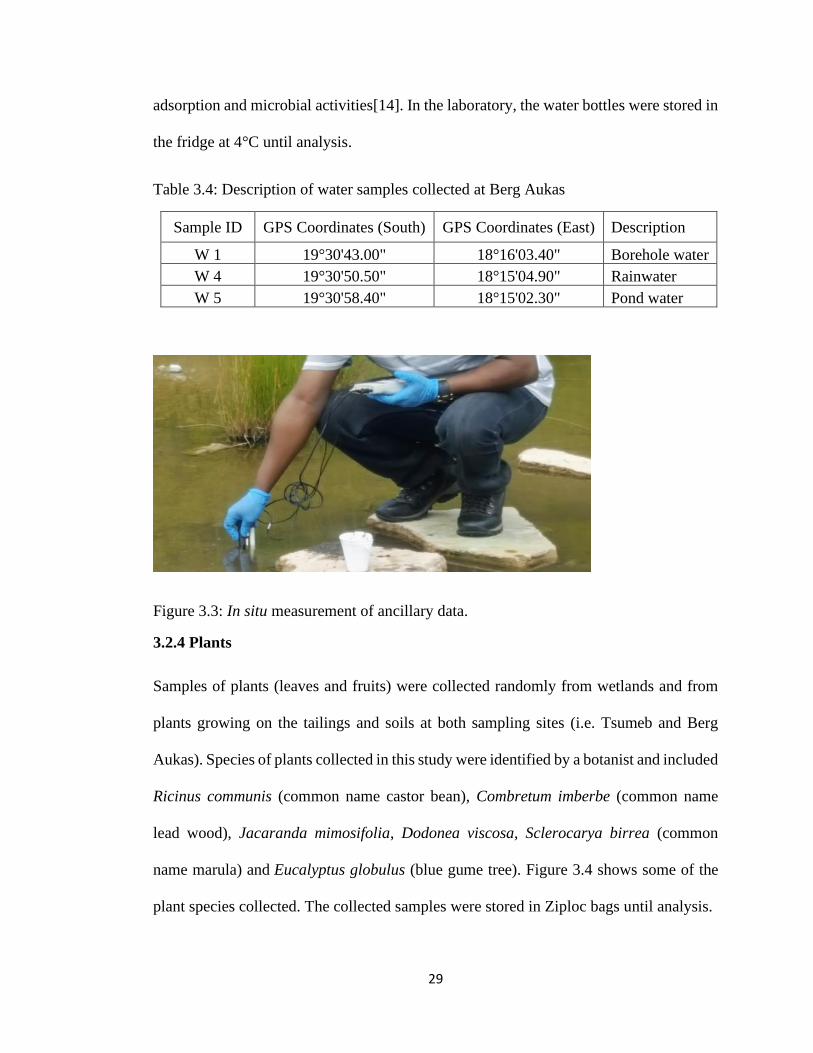
to avoid oxidation of the water sample. Ancillary data such as pH, Ec, ORP, temperature
and turbidity (Figure 3.3) were measured on sites. The samples were processed
immediately at the sampling site by the addition of a small volume of ultra-pure
concentrated HNO3 (Merck) (0.1 to 1% v/v) to one bottle for cations and the other bottle
for anions was not acidified, then both bottles were placed in cooler bags. Adding acid to
water samples maintains the pH < 2 in order to minimize any kinds of precipitation,
29
adsorption and microbial activities[14]. In the laboratory, the water bottles were stored in
the fridge at 4°C until analysis.
Table 3.4: Description of water samples collected at Berg Aukas
Sample ID GPS Coordinates (South) GPS Coordinates (East) Description
W 1 19°30'43.00" 18°16'03.40" Borehole water
W 4 19°30'50.50" 18°15'04.90" Rainwater
W 5 19°30'58.40" 18°15'02.30" Pond water
Figure 3.3: In situ measurement of ancillary data.
3.2.4 Plants
Samples of plants (leaves and fruits) were collected randomly from wetlands and from
plants growing on the tailings and soils at both sampling sites (i.e. Tsumeb and Berg
Aukas). Species of plants collected in this study were identified by a botanist and included
Ricinus communis (common name castor bean), Combretum imberbe (common name
lead wood), Jacaranda mimosifolia, Dodonea viscosa, Sclerocarya birrea (common
name marula) and Eucalyptus globulus (blue gume tree). Figure 3.4 shows some of the
plant species collected. The collected samples were stored in Ziploc bags until analysis.

30
a b
Figure 3.4: Some of the plant species that were collected. (a) Ricinus communis and (b)
Combretum imberbe
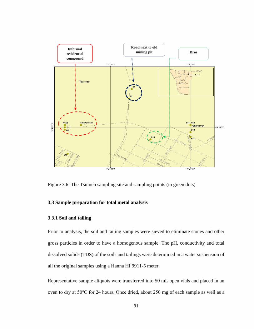
All sampling GPS coordinates were recorded and mapped with a QGIS software (Figures
3.5 and 3.6).
Figure 3.5: The sampling site at Berg Aukas (the blue dots are the sampling points)
Maize
cultivation area Tailing dams Pond wetland/Old
mining site
31
Figure 3.6: The Tsumeb sampling site and sampling points (in green dots)
3.3 Sample preparation for total metal analysis
3.3.1 Soil and tailing
Prior to analysis, the soil and tailing samples were sieved to eliminate stones and other
gross particles in order to have a homogenous sample. The pH, conductivity and total
dissolved solids (TDS) of the soils and tailings were determined in a water suspension of
all the original samples using a Hanna HI 9911-5 meter.
Representative sample aliquots were transferred into 50 mL open vials and placed in an
oven to dry at 50℃ for 24 hours. Once dried, about 250 mg of each sample as well as a
Informal
residential
compound
Road next to old
mining pit Dros

32
Certified Reference Material (CRM), namely BCR 320R Channel Sediment, was
weighed and placed in digestion vessels. To this, analytical grade acid mixture consisting
of 3 ml concentrated HNO3 (Merck), 1 mL concentrated HF (ProMark) as well as 9 mL
concentrated HCl (ProMark) was added. The samples underwent acid digestion in a
closed microwave digestion system (Titan MPS, Perkin Elmer). The parameters of the
digestion method are shown in Table 3.5. Digestion solubilizes particulate matter in the
sample and aids in the removal of potential interferences within the sample matrix [64].
After digestion, the vessels were removed and cooled to room temperature. The digested
samples were placed in glass vials and 6 mL of 4% (v/v) H3BO3 (Merck) was added to
each vial to digest and neutralize the damaging effect of HF to glass. All samples were
stored in the fridge until the day of metal analysis.
Table 3.5: Microwave digestion parameters
T (℃) P (bar) Ramp(min) Hold P (%)
200 30 3 5 90
175 30 2 2 90
50 60 1 2 0
50 60 0 0 0
50 60 0 0 0
33
3.3.2 Plant sample preparation
Plant samples were washed well with tap water, followed by distilled water. This was to
ensure that all the plant samples were free of any dirt and dust. The plant samples were
then left to air dry at room temperature for several days. Once dried, they pruned into
fruits and leaves and were crushed using a mortar and pestle. Between 250 and 300 mg
of each sample and the Certified Reference Material (CRM), namely BCR 482 Trace
Elements in lichens, was weighed and placed in digestion vessels. A mixture of
concentrated HNO3 and HCl in the volume ratio of 3:9 mL was added to the ground plant
samples. The digested samples were stored in the fridge until metal analysis. For total Hg
(HgT), no digestion of the solid samples was required as the instrument and method used
allowed for direct solid measurement.
3.3.3 The characterization of Hg and other metals distribution in affected study
sites
An approved sequential extraction procedure from the Community Bureau of Reference
(BCR) was used to identify the exchangeable, reducible, oxidisable and residue fractions
of Hg as well as other co-occurring heavy metals in soils and tailings. The procedure was
done in the following 4 steps:
Step 1: F1 (Exchangeable): This step aimed at extracting the mobile fraction of Hg as
well as other metals in soil and tailing samples [16]. About 0.1 g of soil, tailing sample
as well as CRM was weighed into 50 mL vials. The weighed solids were mixed with 20
mL of 0.1 M acetic acid (Merck). The mixture was shaken, using a mechanical shaker,
for ± 16 hours at 90 rpm. After shaking, the mixtures were filtered with filter paper (pore
size 125 mm). The supernatant was collected and stored in the fridge at 4°C until analysis

34
with the ICP–OES. The residue was washed with 10 mL distilled water, dried and used
for the next step.
Step 2: F2 (Reducible): This step aims at extracting the contents of each metal that is
bound to oxides of iron and manganese [65]. About 20 mL hydroxylamine hydrochloride
(Sigma-Aldrich) solution was added to the residue from step 1. The mixture was shaken
for about 16 hours using a mechanical shaker. The rest of this step followed the procedure
stated in step 1 above.
Step 3: F3 (Oxidisable): The oxidisable fractions show metals that are bound to sulphur
and organic matter and if conditions become oxidative, these metals will be released into
the environment [65]. About 5 mL of 30% hydrogen peroxide (Merck) was added to the
residue from step 2. The mixture was heated on a hotplate at 65 ± 5°C for 1 hour. Another
5 mL of hydrogen peroxide (Merck) was added and the mixture was heated for an
additional 1 hour at 70 ± 5°C to reduce the volume to less than 1 mL. The residue was
then extracted with 25 mL ammonium acetate (Merck) (adjusted to pH 2). As with step 1
and 2, the mixture was shaken for ±16 hours using a mechanical shaker and then filtered
and stored in the fridge.
Step 4 F4: (Residual): Metals found in this fraction are the most difficult to separate
because they have the strongest association with the crystalline structures [65]. The
amount was calculated by subtracting the total of the first three fractions from the total
amount of metal found in the sample ((Total metal – (F1 + F2 + F3)) = Residual.
In comparison with the selective sequential extraction (SSE) protocol developed by
Bloom et al [56], the following Hg species can be associated to the BCR fractions:
35
Exchangeable (F1): water soluble and acid leachable Hg species such as HgCl2, HgSO4,
HgO and, to a certain extent, CH3Hg+.
Reducible (F2): Hg bound to Fe and Mn oxides, Hg complexed to humic acid and, most
likely, Hg(OH)2.
Oxidisable (F3): strongly complexed Hg species such as the mineral lattice bound Hg,
Hg2Cl2, HgS, and eventually liquid Hg0.
Residue (F4): HgS (cinnabar), m-HgS (meta-cinnabar), HgSe, and HgAu (amalgams).
3.3.4 Leaching procedure for sulphur and anions determination
Sulphur species such as sulphide (S2-), sulphate (SO42-) and organic sulphur are, together
with other anions such as carbonate, chloride and nitrate, important ligands that may
affect metals properties such as mobility. For instance, it is common knowledge that all
metal nitrates and most carbonates are soluble in water whereas metal sulphides have
extremely low solubilities in water. Hence, to understand the distribution of Hg and other
metals in soil (and tailings) it is critical to identify some of the ligands that may play a
role in the behaviour of these metals in a given environment.
A simple sequential leaching process was used to determine the level of anions and total
sulphur in selected soil and tailings from Berg Aukas and Tsumeb. First, about 3.0 g of
the solid samples were mixed with 30 mL of distilled water and shaken for ± 16 hours
with a mechanical shaker. The mixture was then filtered, and the leachate was kept in the
fridge until analysis. This fraction was used to identify the water leachable ligands present

36
in the sample (e.g. sulphate, chloride, nitrate and fluoride) and it is also likely to comprise
the forms of sulphur present in F1 and F2 of the BCR SEP.
The remaining filter cake was then mixed with 30 mL of aqua regia and subjected to the
same treatment as for the water leaching. This fraction was used to determine the
remaining total sulphur content and it is assumed to comprise the hardly soluble forms of
sulphur that are found in F3 and F4 of the BCR SEP.
3.4 Analytical techniques
This section briefly presents the different analytical techniques used in this study.
3.4.1 Mercury analysis of soil, tailings, plant and water
Total Hg (HgT) was determined by directly introducing the samples (i.e. no prior
preparation was required) to an automated mercury analyzer (DMA-80 milestone) shown
in Figure 3.7. This technique employs direct combustion that decomposes the sample in
an oxygen-rich environment and removes any interfering elements [61].
Figure 3.7: The DMA-80 milestone instrument used for total Hg quantification

37
About 0.1g of sample, including CRMs, was weighed into nickel boats using an analytical
balance (Kern). The boats were placed on the instrument auto sampler (Figure 3.8) and
the instrument was started.
Figure 3.8: Nickel boats with samples on the DMA 80 instrument
3.4.2 Elemental analysis of soil, slag tailings, plant and water samples
This was done using an Inductively Coupled Plasma Optical Emission
Spectrophotometer, ICP-OES (Optima 8000, Perkin Elmer), shown in Figure 3.9. ICP-
OES is useful in quantifying the majority of the elements of the periodic table in a variety
of different sample matrices with very low detection limits. Concentrations that can be
detected by the ICP-OES range from trace (5 µg/kg) to very high (mg/kg) [67]. Sample
solutions introduced into the ICP-OES are nebulized and then transferred into a plasma
generated by the radio frequency excitation of argon (Ar) gas [68].

38
Once the sample mist reaches the plasma, it is quickly dried, vaporized and energized
through collisional excitation at high temperature. The plasma emits the atomic emission
which can be viewed in either a radial or axial configuration, collected with a lens or
mirror, and imaged onto the entrance slit of a wavelength selection device. Up to 70
elements can be determined simultaneously [67]. These multi-element determinations are
performed with the combination of a polychromator and an array detector. With regards
to sample throughput and sensitivity, the analytical performance of such systems is
competitive with most other inorganic analysis techniques such as atomic absorption
spectrometry (AAS) especially for sample sensitivity [69].
To calibrate the equipment, working standard solutions in 1% (v/v) HNO3 were prepared
by diluting the stock solution (Mercury and multi-elemental standards, Perkin Elmer)
with distilled water until the desired concentration was achieved. Calibration blanks were
also prepared in 1% (v/v) HNO3.

39
Figure 3.9: Inductively Coupled Plasma Optical Emission Spectrophotometer, ICPOES
(Optima 8000, Perkin Elmer)
All analytical techniques and methods used in this study were validated using appropriate
quality control (QC) standards and certified reference materials (CRMs), respectively.
3.4.3 Determination of anions
Anions such as fluoride (F-), chloride (Cl-), nitrite (NO2-), nitrate (NO3
-) and sulphate
(SO42-) in water leachates from selected soil and tailings were quantified with a Metrohm
(Eco) ion chromatographer (IC). The eluent was a solution of 0.2 mM NaHCO3 and 5.0
mM Na2CO3. A 0.1 M solution of H2SO4 was used as a conductivity suppressor
regenerant solution. Samples were loaded and injected into the IC by means of an auto-
sampler. For calibration, standards of F-, Cl-, NO2-, NO3
- and SO42- were prepared by
accurately diluting, with deionized water, stock solutions prepared from their
corresponding salts, namely NaF (Merck), NaCl (Merck), NaNO2 (Merck), NaNO3

40
(Merck) and Na2SO4 (Merck). Analyses were performed using the parameters presented
in Table 3.6 below.
Table 3.6: IC parameters for the analysis of anions
Flow (mL/min) 1.10
Pressure (MPa) 12.02
T (°C) ±20
Run time (min) 13.0
3.5 Data analysis
Basic Analysis of Variance (ANOVA) was used to statistically compare the reported
mercury concentrations of the used CRMs to the concentrations obtained with the above
proposed methods. These tests are critical for the quality assurance as well as for the
validation of the data that was generated during the study. Correlation analyses was
carried out with the collected data and field measurements, using statistical software such
as the Statistical Package for the Social Sciences (SPSS) to understand the factors
controlling Hg distribution in the samples.
3.6 Research Ethics
Ethical clearance for the study was obtained from the University of Namibia Research
Ethics Committee (UREC) and research permission from the Centre of Postgraduate
Studies (CPGS) (appendix 1).

41
Chapter 4
Results
4.1 Method validation
4.1.1 Total elements
In this chapter, the results of soils, tailings and water from the two sites are presented.
The sites from which the samples were obtained are presented in Chapter 3, Figures 3.5
and 3.6. The different analytical methods used for the quantification of Hg and other
elements were validated using appropriate CRMs. Tables 4.1 and 4.2 show the results
obtained for the triplicate analysis of the CRMs used.
Table 4.1: Elemental concentrations of the CRM used for the validation of soils and
tailings analysis
BCR-320R
Channel Sediment
As
(mg/kg)
Cu
(mg/kg)
Fe
(mg/kg)
Pb
(mg/kg)
Cr
(mg/kg)
Mn
(mg/kg)
Hg
(mg/kg)
Certified ± U 21.7 ± 2.0 46.3 ± 2.9 25700 ± 1300 85 ± 5 59 ± 4 910 ± 50 0.85 ± 0.09
Measured ± SD(*) 23.6 ± 5.0 47.5 ± 2.2 23133 ± 332 90 ± 8 57 ± 3 894 ± 11 0.87 ± 0.06
Recovery (%) 108.8 102.6 90.0 105.9 96.6 98.2 102.3
(*): Results obtained with ICP–OES except for Hg which was analysed by the DMA 80.
U = Uncertainty
SD = Standard Deviation
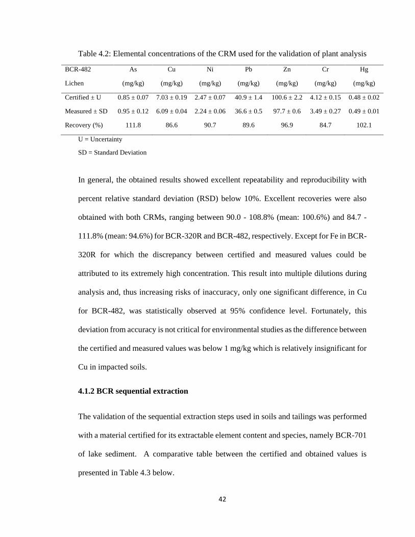
42
Table 4.2: Elemental concentrations of the CRM used for the validation of plant analysis
BCR-482
Lichen
As
(mg/kg)
Cu
(mg/kg)
Ni
(mg/kg)
Pb
(mg/kg)
Zn
(mg/kg)
Cr
(mg/kg)
Hg
(mg/kg)
Certified ± U 0.85 ± 0.07 7.03 ± 0.19 2.47 ± 0.07 40.9 ± 1.4 100.6 ± 2.2 4.12 ± 0.15 0.48 ± 0.02
Measured ± SD 0.95 ± 0.12 6.09 ± 0.04 2.24 ± 0.06 36.6 ± 0.5 97.7 ± 0.6 3.49 ± 0.27 0.49 ± 0.01
Recovery (%) 111.8 86.6 90.7 89.6 96.9 84.7 102.1
U = Uncertainty
SD = Standard Deviation
In general, the obtained results showed excellent repeatability and reproducibility with
percent relative standard deviation (RSD) below 10%. Excellent recoveries were also
obtained with both CRMs, ranging between 90.0 - 108.8% (mean: 100.6%) and 84.7 -
111.8% (mean: 94.6%) for BCR-320R and BCR-482, respectively. Except for Fe in BCR-
320R for which the discrepancy between certified and measured values could be
attributed to its extremely high concentration. This result into multiple dilutions during
analysis and, thus increasing risks of inaccuracy, only one significant difference, in Cu
for BCR-482, was statistically observed at 95% confidence level. Fortunately, this
deviation from accuracy is not critical for environmental studies as the difference between
the certified and measured values was below 1 mg/kg which is relatively insignificant for
Cu in impacted soils.
4.1.2 BCR sequential extraction
The validation of the sequential extraction steps used in soils and tailings was performed
with a material certified for its extractable element content and species, namely BCR-701
of lake sediment. A comparative table between the certified and obtained values is
presented in Table 4.3 below.

43
Table 4.3: Quality control of sequential extraction data using the CRM BCR-701
(n=3,RSD)
n, number of replicates; U (half-width of 95% confidence interval); SD
Of the 12 sets of data examined, only one case (Zn step 2) showed % SD above 10% (i.e.
12.6%) whereas 10 of the 12 data sets had RSD below 5%. Although statistical
differences were observed in a few cases between certified and measured values (e.g. Pb
step 2 and Cd, Cu step 3), this would not affect the significance of the data in terms of
environmental studies due to the closeness of both values at each step [70] and as overall
extracted for each element (e.g. 11.34 mg/kg of Cd is certified to be extractable by the 3
steps and 11.65 mg/kg were actually extracted with the used method).
The obtained data from CRMs analyses for both total elements and sequential extraction,
therefore, showed the reliability of the proposed methods.
Step
Metal
BCR-701 % Recovery
Certified value
mean ± U
(mg/kg)
Obtained value (n=3)
Mean ± SD
(mg/kg)
1 Cd 7.3 ± 0.4 8.6 ± 0.1 117.8
Cu 49.3 ± 1.7 63.8 ± 1.3 129.4
Pb 3.18 ± 0.21 2.98 ± 0.19 93.7
Zn 205 ± 6 230 ± 4 112.2
2 Cd 3.77 ± 0.28 2.98 ± 0.00 79.0
Cu 124 ± 3 140 ± 2 112.3
Pb 126 ± 3 109 ± 3 86.5
Zn 114 ± 5 95 ± 12 83.3
3 Cd 0.27 ± 0.06 0.075 ± 0.01 27.8
Cu 55 ± 4 40 ± 3 72.7
Pb 9.3 ± 2.0 9.6 ± 0.6 103.2
Zn 46 ± 4 46 ± 1 100.0
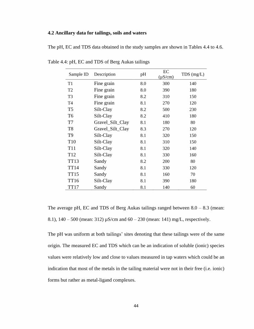
44
4.2 Ancillary data for tailings, soils and waters
The pH, EC and TDS data obtained in the study samples are shown in Tables 4.4 to 4.6.
Table 4.4: pH, EC and TDS of Berg Aukas tailings
Sample ID Description pH EC
(µS/cm) TDS (mg/L)
T1 Fine grain 8.0 300 140
T2 Fine grain 8.0 390 180
T3 Fine grain 8.2 310 150
T4 Fine grain 8.1 270 120
T5 Silt-Clay 8.2 500 230
T6 Silt-Clay 8.2 410 180
T7 Gravel_Silt_Clay 8.1 180 80
T8 Gravel_Silt_Clay 8.3 270 120
T9 Silt-Clay 8.1 320 150
T10 Silt-Clay 8.1 310 150
T11 Silt-Clay 8.1 320 140
T12 Silt-Clay 8.1 330 160
TT13 Sandy 8.2 200 80
TT14 Sandy 8.1 330 120
TT15 Sandy 8.1 160 70
TT16 Silt-Clay 8.1 390 180
TT17 Sandy 8.1 140 60
The average pH, EC and TDS of Berg Aukas tailings ranged between 8.0 – 8.3 (mean:
8.1), 140 – 500 (mean: 312) µS/cm and 60 – 230 (mean: 141) mg/L, respectively.
The pH was uniform at both tailings’ sites denoting that these tailings were of the same
origin. The measured EC and TDS which can be an indication of soluble (ionic) species
values were relatively low and close to values measured in tap waters which could be an
indication that most of the metals in the tailing material were not in their free (i.e. ionic)
forms but rather as metal-ligand complexes.
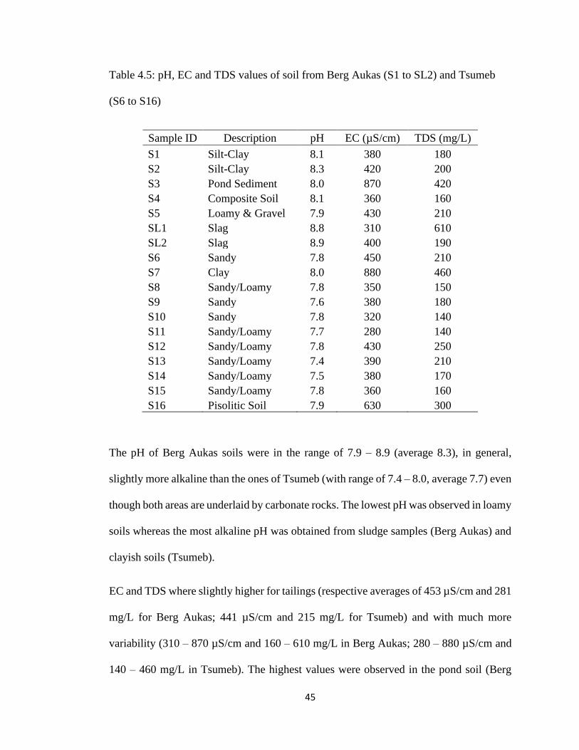
45
Table 4.5: pH, EC and TDS values of soil from Berg Aukas (S1 to SL2) and Tsumeb
(S6 to S16)
Sample ID Description pH EC (µS/cm) TDS (mg/L)
S1 Silt-Clay 8.1 380 180
S2 Silt-Clay 8.3 420 200
S3 Pond Sediment 8.0 870 420
S4 Composite Soil 8.1 360 160
S5 Loamy & Gravel 7.9 430 210
SL1 Slag 8.8 310 610
SL2 Slag 8.9 400 190
S6 Sandy 7.8 450 210
S7 Clay 8.0 880 460
S8 Sandy/Loamy 7.8 350 150
S9 Sandy 7.6 380 180
S10 Sandy 7.8 320 140
S11 Sandy/Loamy 7.7 280 140
S12 Sandy/Loamy 7.8 430 250
S13 Sandy/Loamy 7.4 390 210
S14 Sandy/Loamy 7.5 380 170
S15 Sandy/Loamy 7.8 360 160
S16 Pisolitic Soil 7.9 630 300
The pH of Berg Aukas soils were in the range of 7.9 – 8.9 (average 8.3), in general,
slightly more alkaline than the ones of Tsumeb (with range of 7.4 – 8.0, average 7.7) even
though both areas are underlaid by carbonate rocks. The lowest pH was observed in loamy
soils whereas the most alkaline pH was obtained from sludge samples (Berg Aukas) and
clayish soils (Tsumeb).
EC and TDS where slightly higher for tailings (respective averages of 453 µS/cm and 281
mg/L for Berg Aukas; 441 µS/cm and 215 mg/L for Tsumeb) and with much more
variability (310 – 870 µS/cm and 160 – 610 mg/L in Berg Aukas; 280 – 880 µS/cm and
140 – 460 mg/L in Tsumeb). The highest values were observed in the pond soil (Berg

46
Aukas) and in clayish soil (Tsumeb). One would, therefore, expect much more soluble
forms of metals in the samples from soils than in the tailings.
Table 4.6: pH, ORP and EC of Berg Aukas waters
Sample ID Description pH Eh (mV) EC (µS/cm)
W1(*) Borehole Water 7.4 218 800
W4 Old Pool (Rain) Water 9.0 104 945
W5 Pond Water 8.5 130 512 (*): W1 data, here and elsewhere, are averages of the analysis of 3 borehole samples (W1, W2 and W3)
Water samples, which were only collected in Berg Aukas, also showed considerable
variability, depending on their source, from almost neutral pH (7.4) in borehole waters to
alkaline values, in the rainwater accumulated in an old pool at the camp site (pH = 9.5).
ORP values, on another hand, revealed the predominance of anaerobic conditions at the
site (mean: 151 mV and range: 104 – 218 mV) whereas EC was still low with values
below µS/cm (range: 512 – 945 µS/cm and average: 752 µS/cm).
4.3 Occurrence of total mercury (HgT) in tailings, soils and plants
Figure 4.1 shows examples of the low and high range calibration curves respectively,
obtained with the DMA-80.
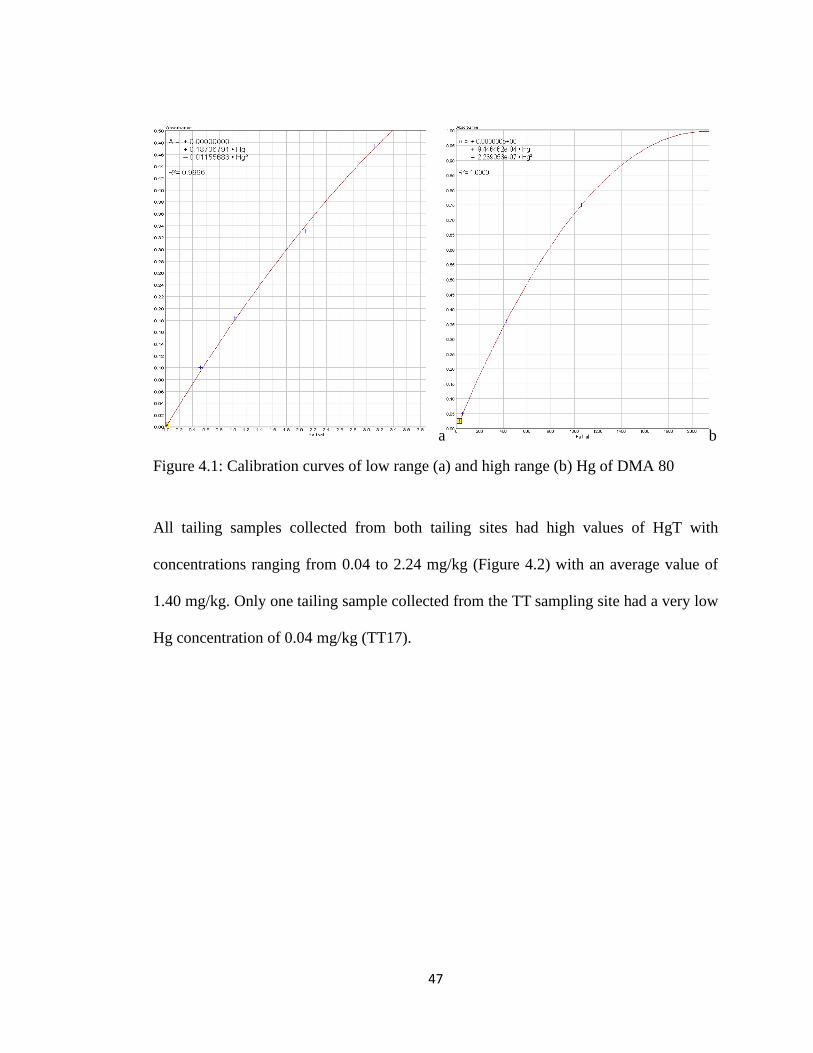
47
a b
Figure 4.1: Calibration curves of low range (a) and high range (b) Hg of DMA 80
All tailing samples collected from both tailing sites had high values of HgT with
concentrations ranging from 0.04 to 2.24 mg/kg (Figure 4.2) with an average value of
1.40 mg/kg. Only one tailing sample collected from the TT sampling site had a very low
Hg concentration of 0.04 mg/kg (TT17).

48
Figure 4.2: HgT in Berg Aukas tailings
Soil samples collected from both Berg Aukas and Tsumeb also showed the occurrence of
HgT with concentrations ranging from 0.02 mg/kg to 3.49 mg/kg and mean concentration
of 0.60 mg/kg (Figure 4.3). Although higher Hg values were generally observed in Berg
Aukas soils, one soil sample that was collected around the vicinity of the Dros restaurant
in Tsumeb (S16) had the highest Hg concentration of all study soils with a value of 3.49
mg/kg. A soil sample (S4), which was collected randomly in Berg Aukas around the
community area, had the second highest concentration of 3.11 mg/kg.
It was also noted that another soil sample (S3) which was collected at the bottom of a
pond wetland near the abandoned mine site in Berg Aukas showed the third highest HgT
value of 2.49 mg/kg.
0.0
0.5
1.0
1.5
2.0
2.5
T1 T2 T3 T4 T5 T6 T7 T8 T9 T10 T11 T12 TT13 TT14 TT15 TT16 TT17
Hg
(mg/
kg)
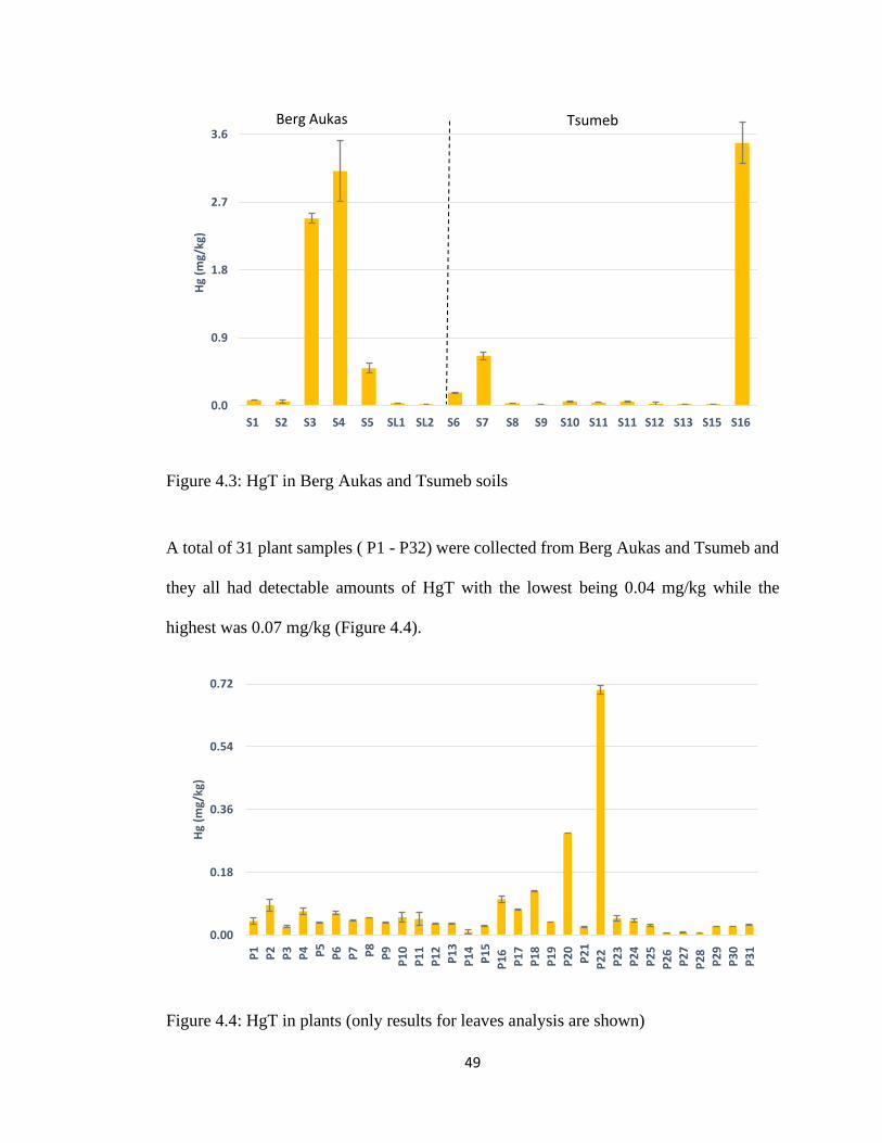
49
Figure 4.3: HgT in Berg Aukas and Tsumeb soils
A total of 31 plant samples ( P1 - P32) were collected from Berg Aukas and Tsumeb and
they all had detectable amounts of HgT with the lowest being 0.04 mg/kg while the
highest was 0.07 mg/kg (Figure 4.4).
Figure 4.4: HgT in plants (only results for leaves analysis are shown)
0.0
0.9
1.8
2.7
3.6
S1 S2 S3 S4 S5 SL1 SL2 S6 S7 S8 S9 S10 S11 S11 S12 S13 S15 S16
Hg
(mg/
kg)
Berg Aukas Tsumeb
0.00
0.18
0.36
0.54
0.72
P1
P2
P3
P4 P5
P6
P7 P8
P9
P1
0
P1
1
P1
2
P1
3
P1
4
P1
5
P1
6
P1
7
P1
8
P1
9
P2
0
P2
1
P2
2
P2
3
P2
4
P2
5
P2
6
P2
7
P2
8
P2
9
P3
0
P3
1
Hg
(mg/
kg)
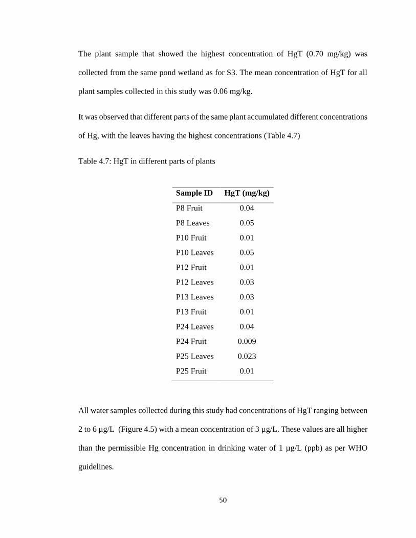
50
The plant sample that showed the highest concentration of HgT (0.70 mg/kg) was
collected from the same pond wetland as for S3. The mean concentration of HgT for all
plant samples collected in this study was 0.06 mg/kg.
It was observed that different parts of the same plant accumulated different concentrations
of Hg, with the leaves having the highest concentrations (Table 4.7)
Table 4.7: HgT in different parts of plants
Sample ID HgT (mg/kg)
P8 Fruit 0.04
P8 Leaves 0.05
P10 Fruit 0.01
P10 Leaves 0.05
P12 Fruit 0.01
P12 Leaves 0.03
P13 Leaves 0.03
P13 Fruit 0.01
P24 Leaves 0.04
P24 Fruit 0.009
P25 Leaves 0.023
P25 Fruit 0.01
All water samples collected during this study had concentrations of HgT ranging between
2 to 6 µg/L (Figure 4.5) with a mean concentration of 3 µg/L. These values are all higher
than the permissible Hg concentration in drinking water of 1 µg/L (ppb) as per WHO
guidelines.

51
Figure 4.5: HgT in Berg Aukas waters
4.4 Occurrence of other heavy metals in Berg Aukas and Tsumeb
4.4.1 Tailings
Generally, Hg and the co-occurrent metals exhibited extremely high concentrations at
both tailing dump sites in Berg Aukas (Figure 4.6). For instance, the concentration of Fe
ranged from 11091 to 37605 mg/kg (mean: 21509 mg/kg), Cu concentrations were
between 142 and 439 mg/kg (mean: 193 mg/kg) whereas Co and Ni were measured at
relatively low amounts with the highest being 5.3 mg/kg (mean: 2.7 mg/kg) and 1.3 mg/kg
(mean: 0.76 mg/kg), respectively.
Moreover, the values for Cd, Mn, Zn, Pb and As ranged from 253 to 422 mg/kg (mean:
320 mg/kg), 289 to 701 mg/kg (mean: 396 mg/kg), 18387 to 38509 mg/kg (mean: 25090
mg/kg), 6679 to 18195 mg/kg (mean: 10045 mg/kg) and 68.2 to 266 mg/kg (mean: 127
mg/kg), respectively.
0
2
4
6
8
W1 W4 W5
Hg
(µg/
L)

52
Most of the tailings had Fe, Al, Zn and Pb concentrations near or greater than the
percentage levels (i.e. ≥ 10,000 mg/kg) as shown in Figure 4.6.
Figure 4.6: Metals and metalloids in Berg Aukas tailings
0
175
350
525
700
T1 T2 T3 T4 T5 T6 T7 T8 T9 T10 T11 T12 TT13 TT14 TT15 TT16 TT17
mg/
kg
Cr Cd Cu Mn As
0
10000
20000
30000
40000
T1 T2 T3 T4 T5 T6 T7 T8 T9 T10 T11 T12 TT13 TT14 TT15 TT16 TT17
Fe Al Zn Pb

53
4.4.2 Soil
Table 4.8 summarises results of heavy metal concentration in soils from Berg Aukas and
Tsumeb. Soil samples collected during this study showed concentrations of Fe ranging
between 6614 and 26769 mg/kg (mean: 14576 mg/kg or 1.5% Fe). Two slag samples
collected at Berg Aukas also showed elevated levels of Fe (mean: 39962 mg/kg or about
4.0% Fe). These two samples also showed elevated concentrations of other heavy metals.
Al and Zn also occurred at or near percentage levels, especially in slag samples, with an
average concentration of 31791 mg/kg (3.2%) and 6144 mg/kg (0.6%), respectively in
soils, and 26630 mg/kg (2.7%) and 19676 mg/kg (2.0%), respectively in slags.
Additionally, toxic metals such as As, Cd and Pb were observed at relatively high
concentrations, especially in Berg Aukas soils. The mean concentration for As was 101
mg/kg, with the highest values measured in soil S4 (298 mg/kg) and slags (mean: 334
mg/kg) from Berg Aukas. The average Cd concentration was 21 mg/kg with the highest
level measured in sample S4 from Berg Aukas (204 mg/kg). Tsumeb soils generally
showed low Cd level, although one sample (S7) had Cd at a concentration of 6.9 mg/kg.
Pb, on the other hand, was measured at concentrations ranging from 8.5 to 18525 mg/kg
(mean: 2050 mg/kg), with the highest concentration measured in sample S4 from Berg
Aukas and lower concentrations observed in soils from Tsumeb. Cr, Cu, Co and Ni also
were present in the study soils though at relatively lower concentrations than the other
metals. The highest concentrations of these elements were measured in Berg Aukas slags
with mean values of 178, 1066, 8.8 and 13.6 mg/kg for Cr, Cu, Co and Ni, respectively.
But, the soil sample with the highest concentration of Cu (S6: 1213 mg/kg) was, in
contrast, collected in Tsumeb. Finally, while soils showed Mn concentrations ranging
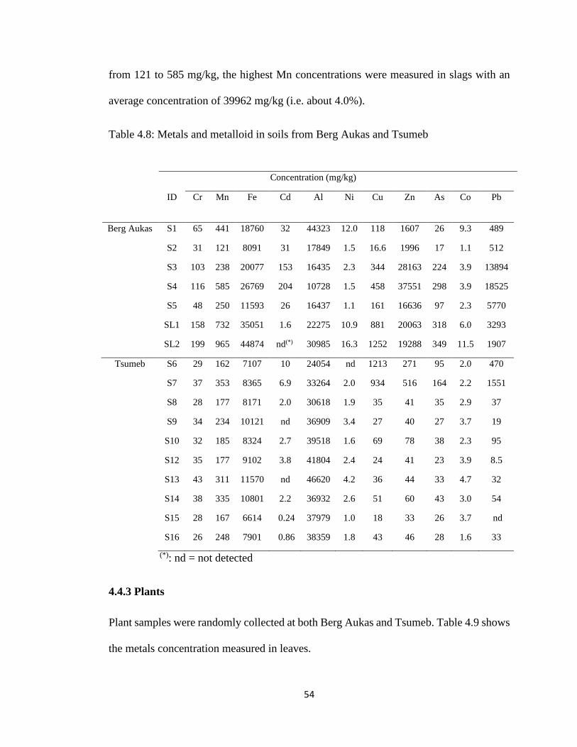
54
from 121 to 585 mg/kg, the highest Mn concentrations were measured in slags with an
average concentration of 39962 mg/kg (i.e. about 4.0%).
Table 4.8: Metals and metalloid in soils from Berg Aukas and Tsumeb
Concentration (mg/kg)
ID Cr
Mn
Fe
Cd
Al
Ni
Cu
Zn
As
Co
Pb
Berg Aukas S1 65 441 18760 32 44323 12.0 118 1607 26 9.3 489
S2 31 121 8091 31 17849 1.5 16.6 1996 17 1.1 512
S3 103 238 20077 153 16435 2.3 344 28163 224 3.9 13894
S4 116 585 26769 204 10728 1.5 458 37551 298 3.9 18525
S5 48 250 11593 26 16437 1.1 161 16636 97 2.3 5770
SL1 158 732 35051 1.6 22275 10.9 881 20063 318 6.0 3293
SL2 199 965 44874 nd(*) 30985 16.3 1252 19288 349 11.5 1907
Tsumeb S6 29 162 7107 10 24054 nd 1213 271 95 2.0 470
S7 37 353 8365 6.9 33264 2.0 934 516 164 2.2 1551
S8 28 177 8171 2.0 30618 1.9 35 41 35 2.9 37
S9 34 234 10121 nd 36909 3.4 27 40 27 3.7 19
S10 32 185 8324 2.7 39518 1.6 69 78 38 2.3 95
S12 35 177 9102 3.8 41804 2.4 24 41 23 3.9 8.5
S13 43 311 11570 nd 46620 4.2 36 44 33 4.7 32
S14 38 335 10801 2.2 36932 2.6 51 60 43 3.0 54
S15 28 167 6614 0.24 37979 1.0 18 33 26 3.7 nd
S16 26 248 7901 0.86 38359 1.8 43 46 28 1.6 33
(*): nd = not detected
4.4.3 Plants
Plant samples were randomly collected at both Berg Aukas and Tsumeb. Table 4.9 shows
the metals concentration measured in leaves.
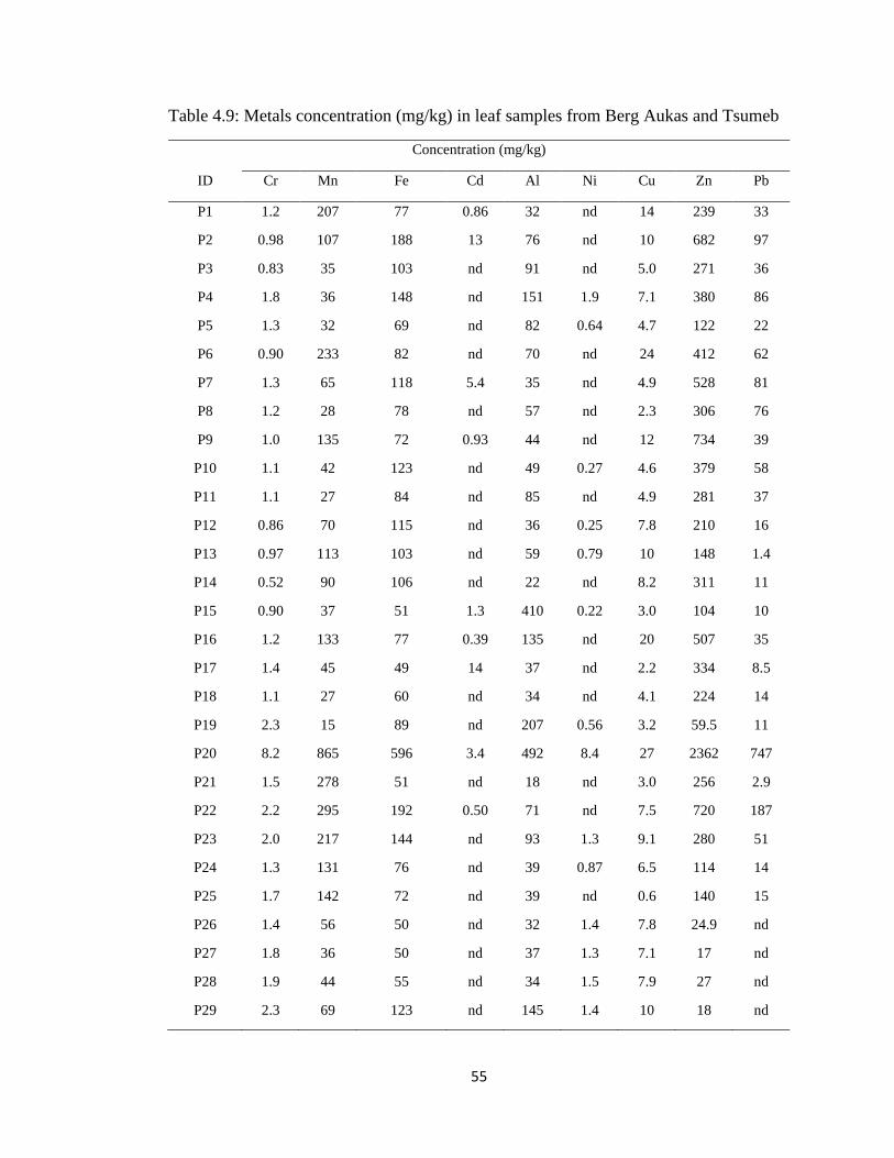
55
Table 4.9: Metals concentration (mg/kg) in leaf samples from Berg Aukas and Tsumeb
Concentration (mg/kg)
ID Cr Mn Fe Cd Al Ni Cu Zn Pb
P1 1.2 207 77 0.86 32 nd 14 239 33
P2 0.98 107 188 13 76 nd 10 682 97
P3 0.83 35 103 nd 91 nd 5.0 271 36
P4 1.8 36 148 nd 151 1.9 7.1 380 86
P5 1.3 32 69 nd 82 0.64 4.7 122 22
P6 0.90 233 82 nd 70 nd 24 412 62
P7 1.3 65 118 5.4 35 nd 4.9 528 81
P8 1.2 28 78 nd 57 nd 2.3 306 76
P9 1.0 135 72 0.93 44 nd 12 734 39
P10 1.1 42 123 nd 49 0.27 4.6 379 58
P11 1.1 27 84 nd 85 nd 4.9 281 37
P12 0.86 70 115 nd 36 0.25 7.8 210 16
P13 0.97 113 103 nd 59 0.79 10 148 1.4
P14 0.52 90 106 nd 22 nd 8.2 311 11
P15 0.90 37 51 1.3 410 0.22 3.0 104 10
P16 1.2 133 77 0.39 135 nd 20 507 35
P17 1.4 45 49 14 37 nd 2.2 334 8.5
P18 1.1 27 60 nd 34 nd 4.1 224 14
P19 2.3 15 89 nd 207 0.56 3.2 59.5 11
P20 8.2 865 596 3.4 492 8.4 27 2362 747
P21 1.5 278 51 nd 18 nd 3.0 256 2.9
P22 2.2 295 192 0.50 71 nd 7.5 720 187
P23 2.0 217 144 nd 93 1.3 9.1 280 51
P24 1.3 131 76 nd 39 0.87 6.5 114 14
P25 1.7 142 72 nd 39 nd 0.6 140 15
P26 1.4 56 50 nd 32 1.4 7.8 24.9 nd
P27 1.8 36 50 nd 37 1.3 7.1 17 nd
P28 1.9 44 55 nd 34 1.5 7.9 27 nd
P29 2.3 69 123 nd 145 1.4 10 18 nd

56
P30 1.8 68 107 nd 138 1.2 7.7 14 nd
P31 2.7 80 205 nd 187 1.6 15 29 1.4
P32 3.2 1.5 65 nd 38 1.0 4.8 nd nd
nd = not detected
As it was the case for Hg, metals accumulation in plants varied according to the location,
the type of plant species and the part of the plant. The obtained mean values for each
identified metal showed the following trend in terms of metal accumulation in leaves: Zn
> Mn > Fe > Al > Pb > Cu > Cd > Cr > Ni. The highest metal levels were recorded in
plants from Berg Aukas with Zn reaching concentration as high as 2362 mg/kg in sample
P20 from the wetland. Sample P20 exhibited the highest values for all the identified
metals.
The majority of the Tsumeb samples had undetected to low metal content in the leaves.
As mentioned above, it also was observed at both sites (Figure 4.7), as for HgT, that
different parts of the same plants accumulated different metals concentrations with the
leaves having the highest concentrations and the lowest in the seeds, indicating an
eventual translocation of the uptaken metals from the roots to the upper part of the plants.
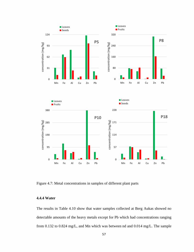
57
Figure 4.7: Metal concentrations in samples of different plant parts
4.4.4 Water
The results in Table 4.10 show that water samples collected at Berg Aukas showed no
detectable amounts of the heavy metals except for Pb which had concentrations ranging
from 0.132 to 0.824 mg/L, and Mn which was between nd and 0.014 mg/L. The sample
0
31
62
93
124
Mn Fe Al Cu Zn Pb
con
cen
trat
ion
(m
g/kg
) P5
LeavesSeeds
0
80
160
240
320
Mn Fe Al Cu Zn Pb
con
cen
trat
ion
(m
g/kg
) P8
LeavesFruits
0
95
190
285
380
Mn Fe Al Cu Zn Pb
con
cen
trat
ion
(m
g/kg
)
P10
LeavesFruits
0
57
114
171
228
Mn Fe Al Cu Zn Pb
con
cen
trat
ion
(m
g/kg
)
P18
LeavesSeeds

58
collected from a pond near the abandoned mine (W5) had presence of Fe, Zn and Pb with
concentrations of 0.281, 1.29 and 0.518 mg/L, respectively.
Table 4.10: Metal concentrations (mg/L) in Berg Aukas waters
ID
Concentration (mg/L)
Mn Fe Pb Zn
W1 nd nd 0.132 0.857
W4 0.003 nd 0.435 nd
W5 0.014 0.281 0.824 1.29
nd = not detected
4.5 Fractionation of mercury in tailings and soils
4.5.1 Mercury fractions in tailings materials
The BCR sequential extraction procedure was used in the study to estimate the amounts
of Hg and other heavy metals in tailing and soil samples, which can be mobilized with
changing environmental conditions [65]. Figure 4.8 shows the extractable fractions of Hg
from the tailing material collected at both tailing sites (i.e. T and TT) in Berg Aukas. The
results obtained showed the occurrence of mainly three fractions: exchangeable (range: 0
- 12.6% and mean: 7.6%), reducible (range: 0 - 4.1% and mean: 0.4%), and residue
(range: 88.0 - 100% and mean: 91.9%. None of the samples had any (or measurable)
oxidisable Hg present whereas the reducible fraction was only observed at site TT in two
samples, namely TT14 and TT15.

59
Figure 4.8: Speciation of Hg in Berg Aukas tailings, (a)T sampling site and (b)TT
sampling site
4.5.2 Hg fractions in soils
Although Hg was found in all four fractions (F1,F2,F3 and F4) of the BCR protocol
(Figure 4.9), only sample S16 from Tsumeb had all the fractions present in it. About 12%
of the Hg in the soil samples from Berg Aukas was exchangeable Hg. Three soil samples
(S2, S4 and S5) showed the presence of the reducible fraction while S1 and S2 showed
37 and 49%, of the oxidisable fraction, respectively. This fraction indicated the amount
of Hg that is bound to sulphur. Should conditions become oxidative, this Hg fraction
could be released to the environment.
While all the analysed soils had a residual fraction averaging at 37 and 41% in Berg Aukas
and Tsumeb, respectively, Hg in sample S3 from a Berg Aukas wetland only occurred as
residual (i.e. 100%).
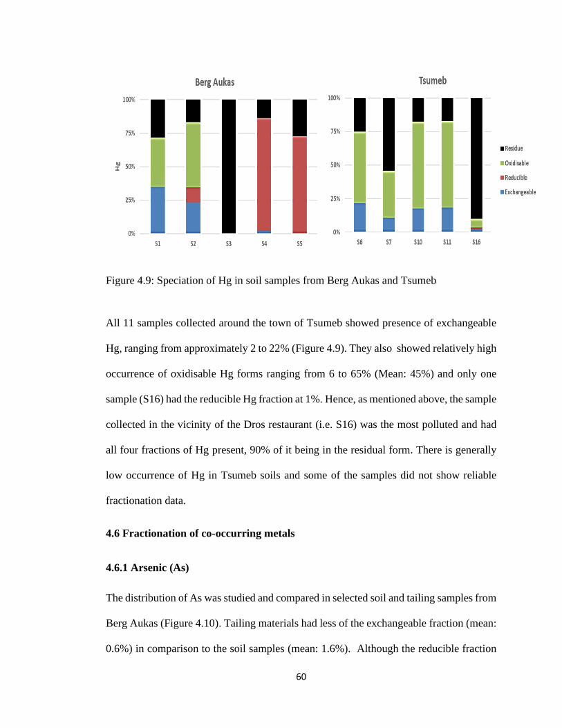
60
Figure 4.9: Speciation of Hg in soil samples from Berg Aukas and Tsumeb
All 11 samples collected around the town of Tsumeb showed presence of exchangeable
Hg, ranging from approximately 2 to 22% (Figure 4.9). They also showed relatively high
occurrence of oxidisable Hg forms ranging from 6 to 65% (Mean: 45%) and only one
sample (S16) had the reducible Hg fraction at 1%. Hence, as mentioned above, the sample
collected in the vicinity of the Dros restaurant (i.e. S16) was the most polluted and had
all four fractions of Hg present, 90% of it being in the residual form. There is generally
low occurrence of Hg in Tsumeb soils and some of the samples did not show reliable
fractionation data.
4.6 Fractionation of co-occurring metals
4.6.1 Arsenic (As)
The distribution of As was studied and compared in selected soil and tailing samples from
Berg Aukas (Figure 4.10). Tailing materials had less of the exchangeable fraction (mean:
0.6%) in comparison to the soil samples (mean: 1.6%). Although the reducible fraction

61
was also present in all samples (mean: 5.3% in soil and 3.3% in tailings), the most
predominant fractions were the oxidisable (mean: 12% in soil and 21% in tailings) and
residual (mean: 81% in soil and 75% in tailings) forms. This indicated that more than
90% of the As found in Berg Aukas soils and tailings occurred in strongly bound forms
in the sample matrices.
Figure 4.10: Speciation of As in Berg Aukas soils and tailings
4.6.2 Cobalt (Co)
The distribution of Co showed that, on average, about 31% (range: 0 to 61%) of the Co
from Berg Aukas was exchangeable and the corresponding amount was 20% (range: 9 to
52%) in Tsumeb soils (Figure 4.11). Here again, the residual fraction was the most
predominant with averages of 53% (range: 3.4 to 99.6%) and 55% (range: 11 to 82%) for

62
Berg Aukas and Tsumeb, respectively. In addition, the majority of Tsumeb soils exhibited
a considerable occurrence of the reducible fraction with a mean of 25% (range: 0 to 44%).
Hg in Berg Aukas soils and Co in sample S3 from the wetland occurred essentially in the
residual fraction (99.6%) with a tiny portion (0.4%) of the exchangeable fraction.
Figure 4.11: Speciation of Co in Berg Aukas and Tsumeb soils
The two tailing collection sites were studied and compared for the distribution of Co. The
results show that both tailing sites had varying amounts of the different fractions of Co
(Figure 4.12). Approximately, 22% of Co in tailings was found in the exchangeable
fraction whereas the Co in the reducible fraction almost counted for 40% of the total Co.
The reducible fraction of Co was present in all the samples collected from both sites at an
average of approximately 38%.

63
Although Co in the oxidisable fraction was quite low (about 1.5%) in the study tailings,
it still reached some considerable values in a few samples such as T6 and T12 which
counted about 9 and 14%, respectively.
Figure 4.12: Speciation of Co in Berg Aukas tailings
4.6.3 Cadmium (Cd)
The fractionation of Cd in soils and tailings revealed the occurrence of relatively elevated
exchangeable forms, with averages of about 22 and 59% in soils from Berg Aukas and
Tsumeb, respectively (Figure 4.13).

64
Figure 4.13: Speciation of Cd in Berg Aukas and Tsumeb soils
While the Cd distribution in Tsumeb soils appeared to have a similar trend with also the
occurrence of the reducible and residual fractions at an average of 21% and 20%,
respectively, there was a slight presence of the oxidisable form in S6 and S7 at 2% and
1%, respectively. Berg Aukas soils showed more variability in its Cd distribution. For
instance, the residual fraction of Berg Aukas soils varied from 11 to 92% from S1 to S5
whereas the exchangeable fraction showed a change between 0.4% (S3) to 38% (S4).
Moreover, while S3, S4 and S5 showed relatively similar amounts of the reducible (44,
41 and 36%, respectively) and oxidisable (28, 8, 21, respectively) forms of Cd, S1 and
S2 showed very little occurrence of these fractions (mean: 2 and 0.5% of reducible and
oxidisable fractions, respectively).
Tailings materials also exhibited a relatively uniform trend with the predominance of the
reducible fraction (45 and 43% on average at T and TT, respectively), followed by the
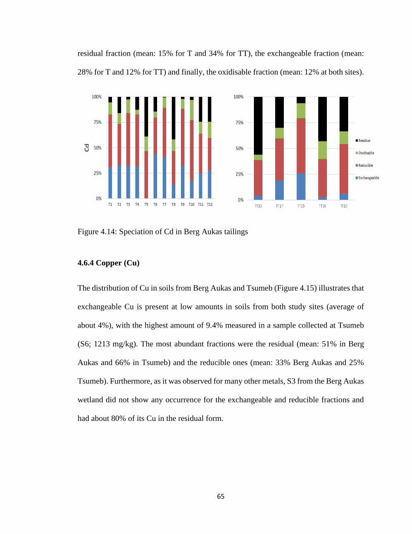
65
residual fraction (mean: 15% for T and 34% for TT), the exchangeable fraction (mean:
28% for T and 12% for TT) and finally, the oxidisable fraction (mean: 12% at both sites).
Figure 4.14: Speciation of Cd in Berg Aukas tailings
4.6.4 Copper (Cu)
The distribution of Cu in soils from Berg Aukas and Tsumeb (Figure 4.15) illustrates that
exchangeable Cu is present at low amounts in soils from both study sites (average of
about 4%), with the highest amount of 9.4% measured in a sample collected at Tsumeb
(S6; 1213 mg/kg). The most abundant fractions were the residual (mean: 51% in Berg
Aukas and 66% in Tsumeb) and the reducible ones (mean: 33% Berg Aukas and 25%
Tsumeb). Furthermore, as it was observed for many other metals, S3 from the Berg Aukas
wetland did not show any occurrence for the exchangeable and reducible fractions and
had about 80% of its Cu in the residual form.
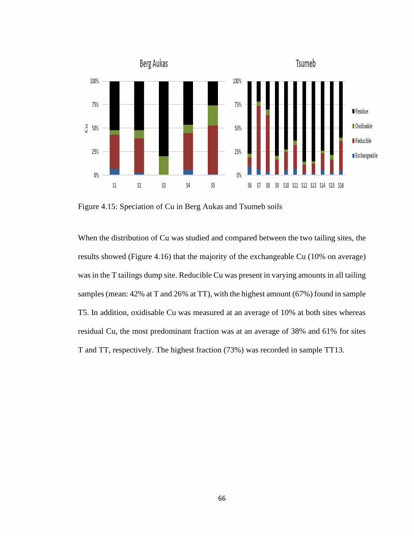
66
Figure 4.15: Speciation of Cu in Berg Aukas and Tsumeb soils
When the distribution of Cu was studied and compared between the two tailing sites, the
results showed (Figure 4.16) that the majority of the exchangeable Cu (10% on average)
was in the T tailings dump site. Reducible Cu was present in varying amounts in all tailing
samples (mean: 42% at T and 26% at TT), with the highest amount (67%) found in sample
T5. In addition, oxidisable Cu was measured at an average of 10% at both sites whereas
residual Cu, the most predominant fraction was at an average of 38% and 61% for sites
T and TT, respectively. The highest fraction (73%) was recorded in sample TT13.

67
Figure 4.16: Speciation of Cu in Berg Aukas tailings
4.6.5 Lead (Pb)
The fractionation of Pb in soils from Berg Aukas and Tsumeb are shown in Figure 4.17.
All defined fractions of the BCR SEP were observed for Pb in all soil samples studied.
Berg Aukas soils had exchangeable Pb ranging from 4 to 18% (mean: 9%) whereas the
same fraction in soils from Tsumeb ranged from 1 to 36 % (mean: 9.6%). Reducible Pb
was observed in high levels in the soil samples (mean: 58% at both sites), with the highest
amount (73%) found at Tsumeb (S9). Oxidisable Pb was, however, not present in high
amounts. It ranged from 2 to 17% in Berg Aukas (mean: 6%) and from 2 to 27% in
Tsumeb (mean: 13%).

68
Figure 4.17: Speciation of Pb in Berg Aukas and Tsumeb soils
On another hand, all tailings samples with the exception of T5, T7, TT16 and TT17, had
detectable amount of exchangeable Pb between 10 and 33% with an average of 15%
(Figure 4.18). The highest amount of exchangeable Pb was found in sample T3. The
reducible fraction also was present in all tailings and ranged between 15 and 67% (mean:
36%). Although oxidisable Pb was present in all samples, it did not occur in high amounts
i.e. from 3 to 10% with an average of 6%. The residual fraction of Pb had the highest
average (45%) of all fractions with at least six tailing samples containing more than 50%
of this non-soluble fraction of Pb.
Since Pb in Berg Aukas tailings occurred at concentrations beyond the percentage level
(i.e. > 10,000 mg/kg), the exchangeable (bioavailable) fraction of Pb obtained in the
tailings reached values as high as 4926 mg/kg (T6).

69
Figure 4.18: Speciation of Pb in Berg Aukas tailings
4.6.6 Manganese (Mn)
All four fractions of the BCR SEP were observed for Mn in soils from both Berg Aukas
and Tsumeb. The amounts varied between the different fractions, with exchangeable
being present in high amounts and oxidisable present in low fractions (Figure 4.19).
Exchangeable Mn ranged from 11 to 63% in soils from Berg Aukas (mean: 43%). This
fraction of Mn was measured at amounts ranging from 15 to 37% (mean: 29%) of the
total Mn (MnT) in soils from Tsumeb. Furthermore, reducible Mn ranged from 15 to 51%
(mean: 33%) of MnT, with the highest amount found in a sample from Tsumeb (S8).
Oxidisable Mn was measured to be less than 12% in all samples studied averaging to
approximately 4% of MnT.
0%
25%
50%
75%
100%
T1 T2 T3 T4 T5 T6 T7 T8 T9 T10 T11 T12 TT13 TT14 TT15 TT16 TT17
Pb
Exchangeable Reducible Oxidisable Residue

70
Figure 4.19: Speciation of Mn in soils from Berg Aukas and Tsumeb
The Mn fractionation in tailings from Berg Aukas is illustrated in Figure 4.20. These
samples revealed the predominance of the reducible fraction (mean: 41%) with the
highest measuring about 52% (from the first tailing site) of the total Mn present with the
highest record (52%) obtained in T7. The exchangeable Mn (mean: 16%) had its highest
fraction (33%) in TT17. Moreover, oxidisable Mn in tailings ranged between 6% and
23% (mean: 14%) while the residual Mn averaged 29% of MnT and peaked at 45% in
T11.
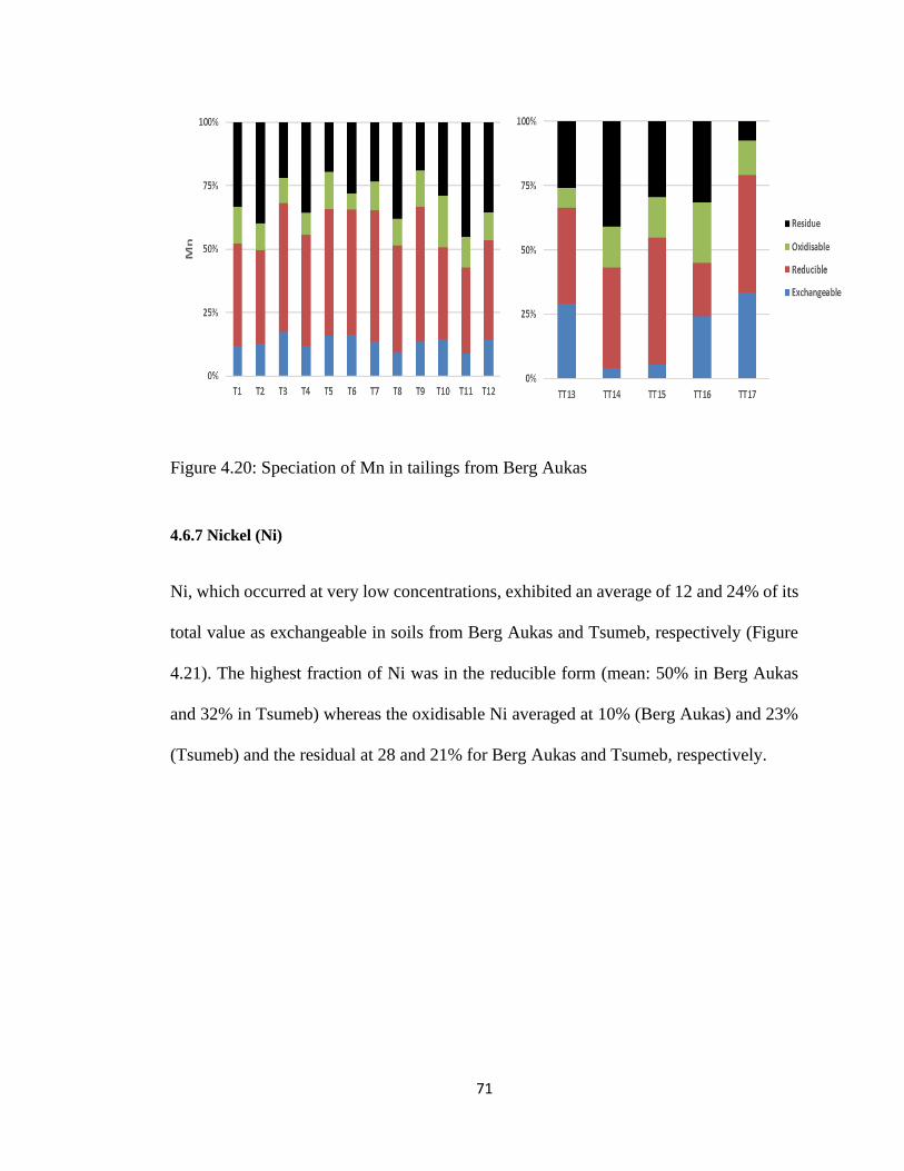
71
Figure 4.20: Speciation of Mn in tailings from Berg Aukas
4.6.7 Nickel (Ni)
Ni, which occurred at very low concentrations, exhibited an average of 12 and 24% of its
total value as exchangeable in soils from Berg Aukas and Tsumeb, respectively (Figure
4.21). The highest fraction of Ni was in the reducible form (mean: 50% in Berg Aukas
and 32% in Tsumeb) whereas the oxidisable Ni averaged at 10% (Berg Aukas) and 23%
(Tsumeb) and the residual at 28 and 21% for Berg Aukas and Tsumeb, respectively.

72
Figure 4.21: Speciation of Ni in soils Berg Aukas and Tsumeb
Ni was not detected at any of the study tailings implying a natural occurrence of this
metal in soils at both sites. This could explain the low values measured in soils.
4.6.8 Zinc (Zn)
Zn occurred at extremely high concentration in Berg Aukas (soils and tailings) as
compared to Tsumeb. As an illustration, the highest concentration of Zn in Berg Aukas
soils in the exchangeable, reducible and oxidisable fractions were 3406 mg/kg (S4), 5883
mg/kg (S4) and 3396 mg/kg (S3), respectively in soil and 3426 mg/kg (T6), 7405 mg/kg
(T6), and 2839 mg/kg (TT17), respectively in tailings. It was observed that all soil
samples in this study had all four fractions present. Two samples from Berg Aukas (S1
and S2) had more than 50% of the exchangeable fraction which averaged at 28% in Berg
Aukas and 18% in Tsumeb (Figure 4.22). The lowest amount of exchangeable Zn in Berg
Aukas (2%) was in S3 from the wetland. Soil samples from Berg Aukas had less reducible
Zn (mean: 17%) in comparison to soil samples from Tsumeb (mean: 30%). The highest
amount (53%) of reducible Zn was found in S7 from Tsumeb. Oxidisable Zn ranged
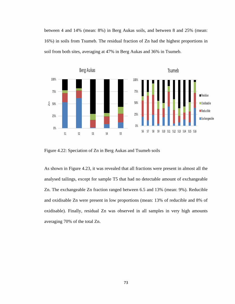
73
between 4 and 14% (mean: 8%) in Berg Aukas soils, and between 8 and 25% (mean:
16%) in soils from Tsumeb. The residual fraction of Zn had the highest proportions in
soil from both sites, averaging at 47% in Berg Aukas and 36% in Tsumeb.
Figure 4.22: Speciation of Zn in Berg Aukas and Tsumeb soils
As shown in Figure 4.23, it was revealed that all fractions were present in almost all the
analysed tailings, except for sample T5 that had no detectable amount of exchangeable
Zn. The exchangeable Zn fraction ranged between 6.5 and 13% (mean: 9%). Reducible
and oxidisable Zn were present in low proportions (mean: 13% of reducible and 8% of
oxidisable). Finally, residual Zn was observed in all samples in very high amounts
averaging 70% of the total Zn.

74
Figure 4.23: Speciation of Zn in Berg Aukas tailings
Overall, the trends observed in the mobile and bioavailable fractions of Berg Aukas and
Tsumeb soils were Mn > Cd > Zn > Pb > Cu > As and Cd > Mn > Zn > Pb > Cu > As,
respectively. Ni did not appear in these sequences due to its extremely low occurrence in
the study soils as mentioned earlier.
4.7 Occurrence of sulphur and anions in soils and tailings materials
Figure 4.24 shows examples of standard chromatogram and calibration lines obtained
during IC analysis.
0%
25%
50%
75%
100%
T1 T2 T3 T4 T5 T6 T7 T8 T9 T10 T11 T12 TT13 TT14 TT15 TT16 TT17
Zn
Exchangeable Reducible Oxidisable Residue
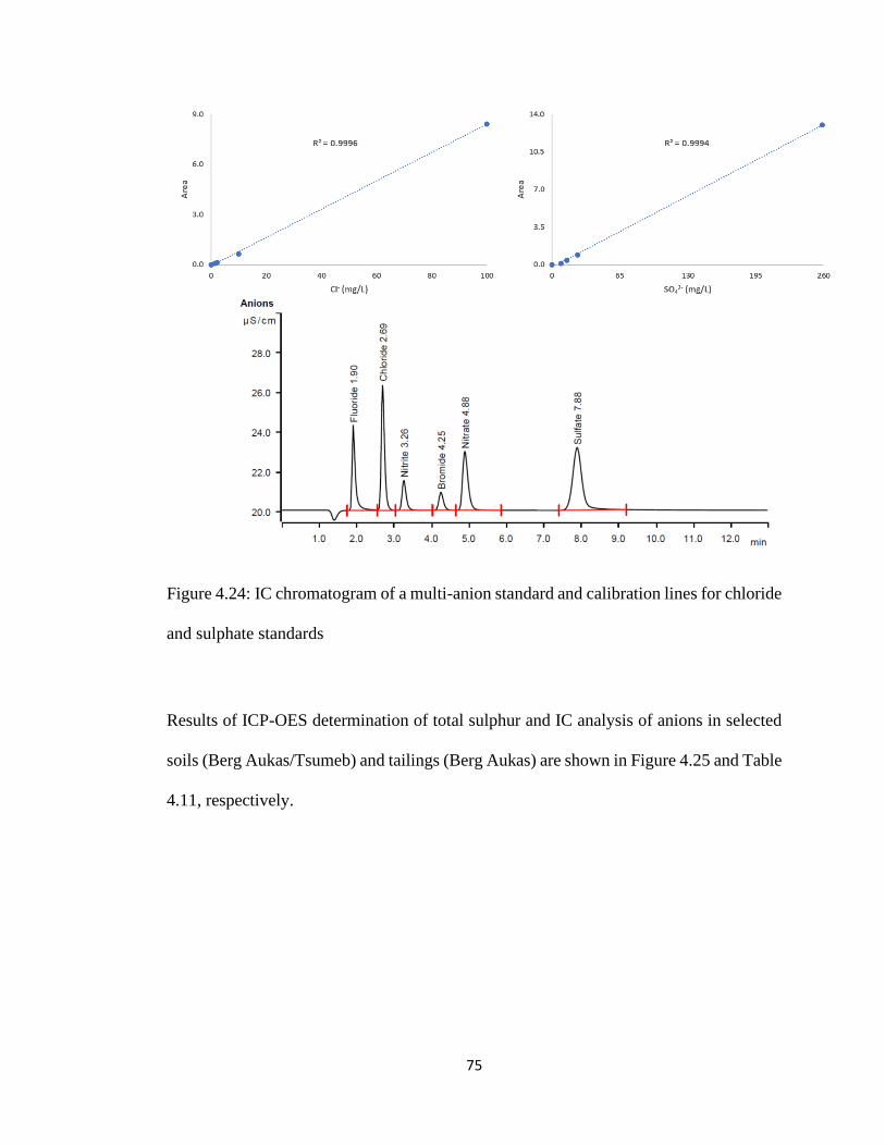
75
Figure 4.24: IC chromatogram of a multi-anion standard and calibration lines for chloride
and sulphate standards
Results of ICP-OES determination of total sulphur and IC analysis of anions in selected
soils (Berg Aukas/Tsumeb) and tailings (Berg Aukas) are shown in Figure 4.25 and Table
4.11, respectively.

76
Figure 4.25: Total sulphur in soils, slags and tailings
The concentrations of sulphur in soil and tailings samples were relatively uniform and
averaged at 6385 mg/kg in soils (range: 5285 to 6736 mg/kg) and 7165 mg/kg in tailings
(range: 6574 to 7723 mg/kg). Additionally, Berg Aukas slags had similar total sulphur
levels as for the tailings with SL1 and SL2 showing sulphur concentrations as high as
7310 and 7469 mg/kg, respectively.
The IC data, on another hand, revealed that sulphate was the most predominant anion in
both soils (mean: 1305 mg/kg) and tailings (mean: 1426 mg/kg), followed by chloride
(mean: 769 mg/kg in soil and 760 mg/kg in tailings), nitrate (mean: 139 mg/kg in soil and
61 mg/kg in tailings), fluoride (mean: 6.5 mg/kg in soil and 8.3 mg/kg in tailings) and
nitrite (Table 4.11).
0
2000
4000
6000
8000
S1 S2 S4 S5 S16 SL1 SL2 T1 T7 T9 TT14 TT15
S (m
g/kg
)
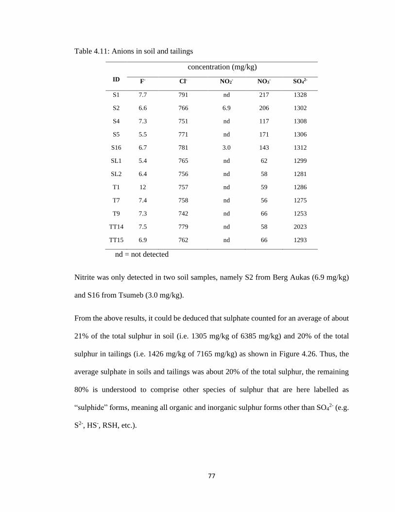
77
Table 4.11: Anions in soil and tailings
ID
concentration (mg/kg)
F- Cl- NO2- NO3
- SO42-
S1 7.7 791 nd 217 1328
S2 6.6 766 6.9 206 1302
S4 7.3 751 nd 117 1308
S5 5.5 771 nd 171 1306
S16 6.7 781 3.0 143 1312
SL1 5.4 765 nd 62 1299
SL2 6.4 756 nd 58 1281
T1 12 757 nd 59 1286
T7 7.4 758 nd 56 1275
T9 7.3 742 nd 66 1253
TT14 7.5 779 nd 58 2023
TT15 6.9 762 nd 66 1293
nd = not detected
Nitrite was only detected in two soil samples, namely S2 from Berg Aukas (6.9 mg/kg)
and S16 from Tsumeb (3.0 mg/kg).
From the above results, it could be deduced that sulphate counted for an average of about
21% of the total sulphur in soil (i.e. 1305 mg/kg of 6385 mg/kg) and 20% of the total
sulphur in tailings (i.e. 1426 mg/kg of 7165 mg/kg) as shown in Figure 4.26. Thus, the
average sulphate in soils and tailings was about 20% of the total sulphur, the remaining
80% is understood to comprise other species of sulphur that are here labelled as
“sulphide” forms, meaning all organic and inorganic sulphur forms other than SO42- (e.g.
S2-, HS-, RSH, etc.).

78
Figure 4.26: Sulphate versus sulphide in soils and tailings from Berg Aukas and Tsumeb
0%
25%
50%
75%
100%
S1 S2 S4 S5 S16 SL1 SL2 T1 T7 T9 TT14 TT15
Sulphide Sulphate

79
Chapter 5
Discussion
5.1 Occurrence of total mercury
HgT was found at high levels in Berg Aukas tailings with a mean concentration of 1.40
mg/kg which was lower than the one of 2.23 mg/kg reported by Mapani et al [33] for the
same site. The observed difference can be attributed mainly to the number of samples
analysed, 17 in this study and 6 in the study conducted by Mapani et al [33], and to a
certain extent, to the season when the different sampling campaigns were carried out.
Higher Hg values are expected to be observed during dry season as leaching processes
would normally reduce metals load at the surface of tailings during rainy seasons.
Furthermore, a study done in South Africa on tailings reported HgT ranging between 0.89
to 6.75 mg/kg [47]. These concentrations, although higher, are still in line with the range
of 0.82 to 2.24 mg/kg measured for Berg Aukas tailings. However, the range reported
here does not include sample TT17 (HgT: 0.04 mg/kg) which was statistically excluded
as an outlier.
On another hand, although both Berg Aukas and Tsumeb soils showed some cases of
extremely high Hg contents, concentrations in Berg Aukas (surface) soils were more
variable than in Tsumeb (Figure 5.1).
This variability could be an indication of either different point sources of pollution or Hg
mobility causing its dispersion in the study area. The expected Hg mobility could be
caused by wind dispersal from the tailings or the Hg was wind-blown in the soils during
the roasting of ores when the mine was still operative.
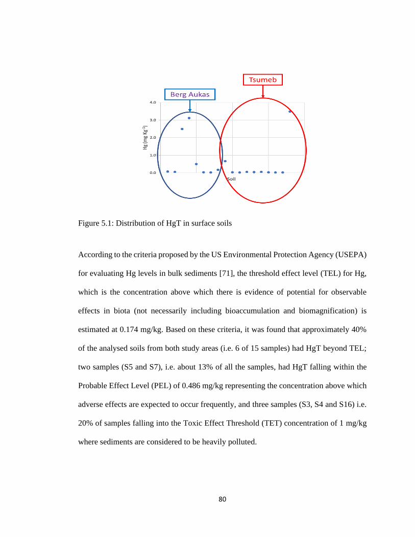
80
Figure 5.1: Distribution of HgT in surface soils
According to the criteria proposed by the US Environmental Protection Agency (USEPA)
for evaluating Hg levels in bulk sediments [71], the threshold effect level (TEL) for Hg,
which is the concentration above which there is evidence of potential for observable
effects in biota (not necessarily including bioaccumulation and biomagnification) is
estimated at 0.174 mg/kg. Based on these criteria, it was found that approximately 40%
of the analysed soils from both study areas (i.e. 6 of 15 samples) had HgT beyond TEL;
two samples (S5 and S7), i.e. about 13% of all the samples, had HgT falling within the
Probable Effect Level (PEL) of 0.486 mg/kg representing the concentration above which
adverse effects are expected to occur frequently, and three samples (S3, S4 and S16) i.e.
20% of samples falling into the Toxic Effect Threshold (TET) concentration of 1 mg/kg
where sediments are considered to be heavily polluted.

81
It was observed that the background Hg values in uncontaminated areas were relatively
low, in the range of 0.015 to 0.055 mg/kg which agrees with the background value of
0.060 mg/kg reported by Hornberger et al [72], which is lower than the generally accepted
natural background for soils of 0.1 mg/kg [73].
Moreover, the study conducted by Mapani et al [33] reported Hg concentrations in soils
from Berg Aukas reaching up to a maximum value of 6.9 mg/kg, a value higher than any
value reported in this study for Berg Aukas soils. Water runoff and other dispersion
mechanisms such as wind which are believed to be responsible of the Hg mobility in the
area could also explain the changes in Hg loads in surface soils. However, Mapani et al.
[33] mainly attributed the elevated Hg levels observed in their study in upper soils to in
situ roasting of fossil fuel as Hg is known to represent highly volatile products of ore
roasting and smelting. Sample S4, collected from the area of old mining operations in
Berg Aukas exhibited the highest HgT suggesting that past roasting operations could be
the principal cause of Hg deposition in the proximity of the old smelter. Additionally,
elevated Hg and other metals were also observed in wetland soil (S3). This is believed to
be the consequence of the drainage of contaminated particles from pollution sources.
In Tsumeb, two samples (S6 and S7) showed high concentrations of HgT. The high
concentrations could be attributed to the fact that these samples were collected alongside
the road near the old Tsumeb open pit mine. Additionally, the sample collected from the
area of the Dros restaurant had a total Hg concentration of 3.49 mg/kg, a value that is
dangerously high. This might indicate the presence of an ore body in the vicinity where
the sample was collected. Cinnabar, a sulphide of Hg, is known to occur naturally in the
ores of the Tsumeb deposit. All the above-mentioned samples were collected from areas

82
that are close to human settlement with constant movement of people, thus posing a high
exposure risk.
Finally, Berg Aukas slag samples (i.e. SL1 and SL2) had a mean HgT of 0.027 mg/kg,
similar to the one of 0.028 mg/kg reported by Mapani et al [33].
HgT measured in both surface and borehole waters in Berg Aukas exceeded international
criteria for Hg in water, such as the World Health Organization Guideline Value (WHO
GV) for drinkable water of 1 μg/L [74] and the USEPA Maximum Contaminant Level
(MCL) of Hg in drinking water of 2 μg/L [75]. Berg Aukas waters had Hg values similar
to those encountered in streams draining areas with concentrated geologic sources of Hg
or with large accumulation of Hg-contaminating tailings from Hg or Au mining [76]. The
highest HgT was measured in borehole samples (W1 to W3: mean Hg: 6 μg/L). These
findings are in line with the observation made by Kortatsi [77] during his study of several
boreholes near the Ankora River Basin (Ghana) that is affected by gold mining. The study
correlated HgT in the wells to the wet season recharge regimes of polluted surface water
and concluded that the occurrence of Hg in the groundwater bodies was largely due to
contamination from surface sources. Similar observations were made by Lusilao et al [78]
in the study of borehole waters from the Vaal River gold mine in South Africa. An
alternate explanation would be that the borehole is sited in a fractured zone of the primary
ore body at Berg Aukas, which contains sulphides of Zn, Pb, V and Hg. This was observed
at Farm Dornhugel, some 60 km west of Berg Aukas, whose borehole water contained
sulphides of Zn, Pb and minor As. This borehole was sited directly through the ore zone
of the Berg Aukas formation [79]. Boreholes (groundwater) are a source of drinking water
in the Berg Aukas area and also water for agricultural and other domestic purposes.

83
Although Hg in Berg Aukas waters showed concentrations that are worrisome, other
physico-chemical parameters of these waters (e.g. pH and EC) fell within the A category
(i.e. excellent quality) of the Namibian Guideline Values for drinking water [79]. On the
Eh-pH diagram of Hg species (Figure 5.2), elemental Hg (Hg0) is likely to be the
predominant species in Berg Aukas waters.
Figure 5.2: Eh-pH diagram of Berg Aukas waters (The red arrows show the exact points
of the Eh-pH values for the corresponding samples)
Since the conditions, at the time of the sampling (late rainy season or fall) were quite
reducing, it is believed that under oxidizing conditions (summer) Hg0 may be converted
to higher oxidation state (e.g. Hg2+) where complex transformation may affect its mobility
and ultimate fate in the environment [80,81].
Plants absorb Hg from air, water and soil through their roots and leaves. The source of
Hg, its chemical form as well as the physiology of the plant species are all factors that
may affect the amount of Hg found in plants [39]. All plants analysed in this study had

84
HgT concentrations of less than 1 mg/kg. The mean Hg value obtained in this study was
0.058 mg/kg, which is slightly higher than that obtained in a study by Soltani et al [82]
which reported a mean Hg concentration of 0.04 mg/kg in plants.
The lowest concentration of Hg in this study (i.e. 0.004 mg/kg) was recorded in
Sclerocarya birrea from Tsumeb. Eucalyptus plant collected at Tsumeb had a mean Hg
concentration of 0.007 mg/kg, which is much lower than the mean concentration (0.081
mg/kg) of Eucalyptus collected at the Rietfontein landfill in South Africa as reported by
Lusilao [39].
A plant (P22) sample collected from a pond wetland (where S3 was collected) had the
highest recorded amount of HgT of 0.703 mg/kg. Studies have shown that the uptake of
Hg tends to be plant specific, with plants like lichens, woody plants, crop plants and
wetland plants known to take up a lot of Hg [19].
Heavy metal transfer from soil to plant is dependent on the plant species and metal type.
Once heavy metals have accumulated in the soil, there are several factors that may
influence the transfer of metals to plants. These factors include total concentration of
metals, specific geochemical form, and chemical speciation of metals, pH, EC, redox
states and soil organic matter (SOM) [82]. Properties of soil such as texture, pH-value,
and ion exchange capacity have a strong influence on the availability of metals to plants.
Even though Hg is strongly fixed in soils, if conditions allow, it can be absorbed by plants.
To quantify the amount of heavy metal that a plant can take up from the soil its growing
in, the transfer coefficient (TC), which is a function of both soils and plant properties,
must be determined.

85
The TC is given by the expression below [83]:
TC = Cplant/ Csoil (5.1)
where Cplant is the concentration of the metal in the plant and Csoil is the concentration of
the metal in the soil.
Table 5.1 summarises the TC of four plants that were collected at the same area as S3 in
Berg Aukas. Only one of the four plant species was identified. The TC of Hg in
unimpacted soils ranges between 0.01 and 0.1 [84]. Two plants, P20 and P22, exceeded
this range, with a TC of 0.118 and 0.283, respectively. This means that there is more Hg
available for uptake by the plant. These values are however low, compared to TC values
obtained by Lusilao [39] in Rietfontein (South Africa) that were 0.743 and 0.882 for two
Eucalyptus plant species. The same study reported TC values of 0.053 and 0.102 in two
algae plants from Randfontein, with the former having a value equivalent to the TC in
Combretum imberbe in the present study. A study conducted in Ethiopia by Duressa and
Leta [85] reported TC values ranging from 0.112 to 0.266 for Hg in vegetables, which is
a smaller range than the one from the present study. Duressa and Leta [85] also found that
if the pH of the soil is higher than 6.5, adsorption of metals to soil is usually very high
and only traces of the element will be available for uptake by the plant. The pH of the soil
sample (S3) used for the TC calculation was 8.0, thus explaining the low TC values.

86
Table 5.1: Transfer coefficients of mercury for selected plants in Berg Aukas
Soil
ID
Hg
(mg/kg)
Plant
ID
Hg
(mg/kg)
TC
S3 2.487 P16 (unidentified) 0.103 0.041
P18 Combretum imberbe 0.126 0.051
P20 (unidentified) 0.293 0.118
P22 (unidentified 0.703 0.283
TC= Transfer Coefficient
Taking into consideration that some parts of Berg Aukas is used for agricultural purposes,
the TC can be used to predict before planting if it is safe to plant vegetables and crops in
that area based on the concentrations of the heavy metals in soil. A higher TC value
indicates that more of the element is available for accumulation by the plant. However, it
must be noted that the TC alone is not sufficient to conclude on the metal bioavailability
because some of the Hg in the leaves originates from the atmosphere [39].
5.2 Heavy metal concentrations
5.2.1 Soils and tailings
Soils are the reservoir for many harmful constituents, elemental and biological, including
heavy metals [44]. Results for the soil analyses revealed the occurrence of pollution at
both sites, and that soils from Tsumeb had generally lower concentrations of total metal
in comparison to soil samples from Berg Aukas. The Berg Aukas large scale
contamination by heavy metals in soils is likely related to past ore roasting activities and
to water and wind dispersal of fine grain particles from the metal-rich unprotected and
poorly designed tailings dams in the area.

87
Since Namibia has no guidelines on soil quality, the Canadian guidelines [86] were used
for comparison. This study reveals that the soils at Berg Aukas and Tsumeb are highly
polluted according to Canadian soil quality guidelines for land use as shown in Table 5.2
Table 5.2: Canadian soil quality guidelines for protection of environmental and human
health (mg/kg) [86]
Element Land use
Residential Commercial Industrial
Arsenic 12 12 12
Chromium 10 22 22
Cadmium 64 87 87
Copper 63 91 91
Lead 140 260 600
Nickel 50 50 50
Zinc 200 360 360
Mercury 6.6 24 50
Other soil references, such as the measured background metal values in soil collected
from Oshakati, Northern Namibia, (collected during a different study and used as a
negative control in this study) were also used for comparison (Table 5.3) and they all
highlighted the pollution occurring in both areas.

88
Table 5.3: Concentrations (±SD) of trace metals from Oshakati, Northern Namibia,
unpolluted soils and other published mean sediments/soils values (in mg/kg)
Source Cr Mn Ni Cd Cu Zn As Pb
Oshakati (n = 9) 1.3 ± 1.4 10 ± 13 5.0 ± 4.7 ns 7.1 ± 8.4 29 ± 32 0.9 ± 0.8 1.2 ± 1.2
China Type 1(*) 90 ns(***) 40 0.2 35 100 ns 35
China Type III (*) 400 ns 200 1.0 400 500 ns 500
Agricultural (**) ≤350 2000 50 3.0 150 300 20 100
(*): Type I = unpolluted soil & Type III = heavily polluted soil [87]
(**): WHO except for Cr [88] and Ni [89]
(***): not specified
Cd in tailing samples from Berg Aukas had a mean concentration of 320 mg/kg. A study
that aimed at assessing potential human risks associated with historic ore processing at
Berg Aukas found a mean concentration of 352 mg/kg for Cd in tailings [33], which was
slightly higher than the mean concentration found in this study. Moreover, a study
conducted at Rosh Pinah by Kribek et al [63] found a mean concentration of 37 mg/kg
for Cd in the tailings, a value much less than what was reported for Berg Aukas
previously[33] and the current study.
Zn, on the other hand, was observed in very high amounts in tailing samples from Berg
Aukas with a mean concentration of 1476 mg/kg. When Kribek et al [63] studied the soils
from tailing dams in Rosh Pinah, they found a mean value of Zn to be 14030 mg/kg. The
high mean value in Rosh Pinah is attributed to the fact that Rosh Pinah is an active Zn
mine, whereas Berg Aukas has been closed for more than 30 years [60] and large amounts
of minerals has now been dispersed and leached out.
89
The data presented in Tables 5.2 and 5.3 show that the maximum permissible limits were
exceeded for most, if not all, toxic metals except Mn. The high levels recorded indicated
that the area is highly contaminated and unsuitable for agricultural use and may also cause
some adverse health effects. The general trend observed in descending order is Al > Fe >
Zn > Pb > Mn > Cu > Cr > As > Cd > Ni > Co.
Tsumeb soils generally indicated, as mentioned above, much lower heavy metal content
compared to Berg Aukas soils. Most of its soils had Zn and Pb below threshold values,
except for samples S6, S7, S10 and S11, which exceeded the permissible limits. These
four soils were collected in areas with constant human movement (S6 and S7 alongside
the road near the old mining pit, and S10 and S11 in and around an informal residential
area). Exposure to high toxic metal concentrations poses high risk to people living in the
area. Exposure to Pb can affect brain and central nervous system, consequently leading
to death. Cd exceeded the permissible limits reported above in all samples in which it was
detected. Cu and As were also found to exceed the guideline values. The high
concentrations (especially in Cu) can be attributed to the fact that Tsumeb is a Cu mining
town.
Furthermore, research has shown that concentration of metals cannot provide extensive
indications about the state of contamination in soils [90]. For this reason, the enrichment
factors (EF) is usually calculated. The EF is defined as a means of quantifying the
enrichment of a potentially contaminant-derived element in an environmental sample
relative to a user-defined background position [90]. Once EF is calculated, the state of
soil quality can be indicated by different values as seen in Table 5.4.

90
Table 5.4: EF categories [90]
Value Soil dust quality
EF < 2 Deficiency to minimal
enrichment
2 < EF < 5 Moderate enrichment
5 < EF < 20 Significant enrichment
20 < EF < 40 Very high enrichment
EF > 40 Extremely high
enrichment
The EF in this study was calculated for Hg, Pb, Cd, As and Zn and was expressed as
follows:
EF = [Metal/RE]soil / [Metal/RE]background (5.2)
where, RE is the value of metal, adopted as Reference Element.
The mean concentrations of the elements mentioned above were calculated for each site
and used in the above expression (5.2). Table 5.4 shows the classification of EF values.
Soils from Berg Aukas have EF values > 40 for Hg, Cd, As and Zn. These values indicate
that Berg Aukas soils are extremely enriched with these heavy metals (Table 5.4). Onjefu
et al [91] also reported very high EF values (20 < EF < 40) for Cd in sediments from
Walvis Bay. The EF of Pb in Berg Aukas was 0.35, which shows some deficiency to
minimal enrichment. However, in Tsumeb soils the EF for Pb was 88. This value
indicated that Tsumeb soils are extremely rich in Pb. EF for Cd in Tsumeb soils was by
Onjefu [33] reported as 2.9, which indicated that Tsumeb soils are moderately enriched
with Cd. Additionally, the EF values obtained for As and Zn showed significant
enrichment whereas Hg had an EF value of 22, which indicated very high enrichment. A

91
study conducted in South Africa by Okedeyi et al [92] in 2014 reported moderate
enrichment of Hg (2.3 - 4.2) in three coal fired plants, values that are lower than those
obtained in the present study for both Berg Aukas and Tsumeb.
Table 5.5: Enrichment Factors of selected heavy metals in Berg Aukas and Tsumeb soils
Berg Aukas Tsumeb
Soil Background Soil Background
Element Mean
RE
Mean
RE EF Mean RE Mean RE EF
Hg 1.285 12082 0.06 27,954
**
49 0.418 8807 0.06 27,954
**
22
Pb 2342 12082 1.223 2212 0.35 427 8807 1.223 2212 88
Cd* 115 12082 0.857 5192 58 4.23 8807 0.857 5192 2.9
As 438 12082 0.924 2212 87 51.3 8807 0.924 2212 14
Zn 14447 12082 43.3 2212 61 116.9 8807 43.3 2212 0.67
*Cd background values [93]
**Hg RE value [94]
For this study, Fe was used as a reference material for background concentrations in the
earth’s crust. The assumption used is that no anthropogenic activities have disturbed its
content in the crust. Additionally, it is an acceptable element for normalization when
calculating EF values [95]. The correlation coefficients between the total trace metal
concentrations in the study soils are shown in Table 5.6.
A relatively strong positive correlation was found between Fe, As and Cr with all other
metals with the exception of Cd and Al. This may suggest a mineral association between
these metals such as the reported association between Cr, Cu, Ni, Pb and Zn to Fe oxide
minerals (e.g. haematite or magnetite) or to Fe and Mn oxyhydroxide minerals (e.g.
goethite, ferrihydrite, and manganite).

92
Table 5.6: Correlation (Pearson correlation coefficients at P < 0.05) matrix between metal
concentrations in Berg Aukas and Tsumeb soils
Cr Cd Ni Co Al Fe Cu Zn As Pb Hg
Cr 1 Cd -0.003 1 Ni 0.803 -0.246 1 Co 0.824 -0.217 0.965 1 Al -0.327 -0.578 0.149 0.140 1 Fe 0.996 -0.017 0.837 0.854 -0.285 1 Cu 0.616 -0.018 0.416 0.413 -0.357 0.578 1 Zn 0.752 0.452 0.301 0.382 -0.707 0.737 0.390 1 As 0.910 0.120 0.547 0.584 -0.528 0.880 0.763 0.832 1 Pb 0.415 0.488 -0.061 0.047 -0.687 0.402 0.182 0.891 0.590 1
Hg 0.586 0.645 0.286 0.305 -0.552 0.577 0.391 0.735 0.615 0.587 1
There is a good correlation between Hg and Cd, suggesting that they are associated
together in the ores that were mined at Berg Aukas. In Pb-Zn mines, Cd is generally
associated with Pb and Hg. It has also been stated that metals with a highly positive
correlation are possibly from the same pollution source, and metals with a highly negative
correlation (which was not observed in the present study) are possibly from the different
pollution source [96]. An extended correlation analysis between metals in Berg Aukas
tailings and other parameters such as total sulphur and anion contents (Table 5.7) also
revealed strong positive correlations between almost all the analyzed metals (Hg
included), and between metals and total sulphur (ST), sulphate and chloride.
This can be an indication of the predominance of metal sulphide and metal chloride
phases in the tailings. These correlations are further discussed in metal fractionation.
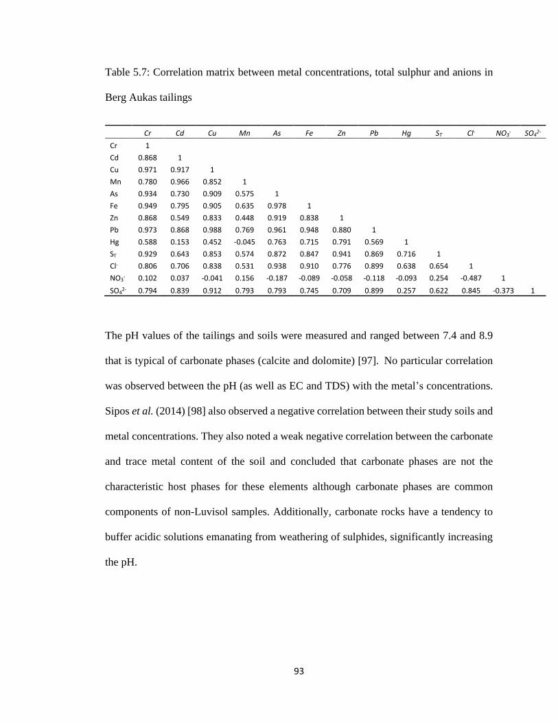
93
Table 5.7: Correlation matrix between metal concentrations, total sulphur and anions in
Berg Aukas tailings
Cr Cd Cu Mn As Fe Zn Pb Hg ST Cl- NO3- SO4
2-
Cr 1 Cd 0.868 1 Cu 0.971 0.917 1 Mn 0.780 0.966 0.852 1 As 0.934 0.730 0.909 0.575 1 Fe 0.949 0.795 0.905 0.635 0.978 1 Zn 0.868 0.549 0.833 0.448 0.919 0.838 1 Pb 0.973 0.868 0.988 0.769 0.961 0.948 0.880 1 Hg 0.588 0.153 0.452 -0.045 0.763 0.715 0.791 0.569 1 ST 0.929 0.643 0.853 0.574 0.872 0.847 0.941 0.869 0.716 1 Cl- 0.806 0.706 0.838 0.531 0.938 0.910 0.776 0.899 0.638 0.654 1 NO3
- 0.102 0.037 -0.041 0.156 -0.187 -0.089 -0.058 -0.118 -0.093 0.254 -0.487 1
SO42- 0.794 0.839 0.912 0.793 0.793 0.745 0.709 0.899 0.257 0.622 0.845 -0.373 1
The pH values of the tailings and soils were measured and ranged between 7.4 and 8.9
that is typical of carbonate phases (calcite and dolomite) [97]. No particular correlation
was observed between the pH (as well as EC and TDS) with the metal’s concentrations.
Sipos et al. (2014) [98] also observed a negative correlation between their study soils and
metal concentrations. They also noted a weak negative correlation between the carbonate
and trace metal content of the soil and concluded that carbonate phases are not the
characteristic host phases for these elements although carbonate phases are common
components of non-Luvisol samples. Additionally, carbonate rocks have a tendency to
buffer acidic solutions emanating from weathering of sulphides, significantly increasing
the pH.

94
5.2.2 Plants
Plants are known to take up and accumulate trace metals from contaminated soil. The
results of the analysis of heavy metals in plants for the present study revealed that the
mean concentration of Mn in Berg Aukas plants was 136.2 mg/kg while Tsumeb had a
mean concentration of 50.6 mg/kg. A study conducted by Ho et al [99] in 2013 found the
mean concentration of Mn to be 69.4 mg/kg. Background concentration of Mn in grass is
in the range of 17 to 334 mg/kg [100]. The values obtained in this study for both Berg
Aukas and Tsumeb fall within this range (17- 334 mg/kg).
On another hand, Cd was not detected in plant samples in Tsumeb but a mean
concentration of 4.53 mg/kg was reported in plants from Berg Aukas. This mean was
slightly higher than that of 0.1 mg/kg reported in Nigeria from a study conducted by
Ogundele et al [101] in plants from Shao, while plants from Asomu, Okolowo, Idofian,
Ganmo, Olooru all had Cd mean below 0.028 mg/kg. The same study reported mean
concentration of Cd to be 0.40 and 0.35 mg/kg in plant samples from Elemere and Jebba,
respectively. According to WHO [102], the recommended permissible limit of Cd in
plants is 0.02 mg/kg. Additionally, all the plant samples analysed in the present study had
Cd above the permissible limit, thus indicating contamination.
Results also showed high levels of Zn in plants from Berg Aukas and Tsumeb with the
mean concentration of 404.1 and 21.7 mg/kg, respectively. The average Zn concentration
in plants at Berg Aukas is almost 400 times higher than the permissible limit allowed by
the WHO [102] for plants of 0.6 mg/kg. This high amount can be attributed to the fact
that Berg Aukas was a Zn mine. The concentrations of Zn in plants growing on mine

95
tailings in central Mexico were reported to be 51.3 and 102.8 mg/kg in roots and shoots,
respectively [103].
The plants collected in Tsumeb exhibited low levels of Pb, with only one sample (P31),
identified as Sclerocarya birrea (common name Marula tree), showing Pb with an amount
of 1.4 mg/kg, a concentration below the WHO permissible concentration of 2 mg/kg. A
study conducted in Ethiopia by Duressa et al [85] reported mean Pb concentrations of
0.62, 0.30, 0.37, 0.69 and 0.60 mg/kg in garlic, kale, onion, pepper and potato,
respectively. These low values of Pb can be attributed to the fact that plants, in general,
are less likely to absorb or accumulate Pb due to its low bioavailability, But, if these plants
are grown in soils with high levels of Pb, it is possible for some Pb to be taken up.
Therefore, poisoning of Pb from plants is usually from Pb-containing dust particles that
settles on plant surfaces rather than the uptake of Pb by plants [104].
Ricinus communis is a medicinal plant that grow in soils with high concentrations of
heavy metals [105]. This plant species was commonly found vegetating the mine tailings
that showed high levels of heavy metals in Berg Aukas. Only one of the three samples of
this species had detectable Cd (1.3 mg/kg) which is low compared to the Cd concentration
of 13 mg/kg found in a study conducted by González-Terreros et al [105] in Mexico. On
the other hand, Mn, Zn and Pb mean concentrations were reported to be 80, 187 and 7.5
mg/kg, respectively. In a study conducted on the same plant species growing on
contaminated sites in industrial areas of the Islamabad and Rawalpindi by Nazir et al in
2011 [106],the mean concentrations of Zn and Pb were 48 and 20 mg/kg, respectively.
Additionally, another plant species that is commonly found in Berg Aukas tailings and
wetland is Combretum imberbe, also a medicinal plant. The mean levels of Pb and Zn

96
reported in this study were high (36 mg/kg for Pb and 227 mg/kg for Zn) compared to
mean levels obtained in the same plant species by Dzomba et al [107] in central
Zimbabwe, where mean concentrations of Pb and Zn were reported to be of 0.56 and 0.30
mg/kg, respectively.
The results showed that different parts of a plant absorb and accumulates heavy metals
differently. The general trend was that leaves of a plant tended to accumulate higher
concentrations of heavy metals in comparison to the fruits of the same plant. This may be
explained by the mechanism adopted by plants to remove heavy metals from the plant via
leaf shedding every year [108]. A plant sample (P20) collected in a pond wetland at Berg
Aukas measured high concentrations of most heavy metals studied (Table 4.10. These
high concentrations can be due to the fact that wetlands are known to have an ability to
accumulate heavy metals (thus they are called “sink of pollutants’’) [109]. Besides, the
corresponding soil sample (S3) showed little or none of the exchangeable fraction for all
the metals, meaning all the likely existing F1 could already have been transferred into the
supernatant water (since it is water soluble) thus facilitating the uptake of this bioavailable
fraction by the wetland plants. Simply, there is likely high amounts of soluble,
bioavailable metals in the pond.
5.3 Distribution and fractionation of mercury
The speciation of Hg, which includes most phase minerals, secondary phases, gaseous
and aqueous species, is very important to assess the Hg transport (i.e. mobilisation) and
impact in the environment. For instance, the incidental ingestion of contaminated soils is
thought to be one of the main terrestrial exposure pathways to metal burdens in the human
body. Often, the total soil metal concentration has been assumed to represent the

97
bioavailable dose, but as mentioned earlier, it is well known that inorganic (IHg),
elemental (Hg0), and organic Hg (RHgX) have different chemical and physical properties,
routes of exposure and toxicological effects. Hence, the form of ingested Hg is important
to assess the absorbed dose. Elemental speciation, therefore, provides important data to
predict metal bioavailability that appears to be site, media and matrix specific.
Tailings and soils from Berg Aukas and Tsumeb were subjected to sequential extraction
to study Hg and other metals distribution and forms of occurrence. As stated earlier, Hg
in tailings mainly occurred in the residual (non-soluble) fraction, i.e. F4 at about 92% of
the HgT while the exchangeable (F1) and reducible (F2) fractions counted for 7.6 and
0.4%, respectively.
The variability observed in Hg fractionation in soils from Berg Aukas and Tsumeb
illustrates the matrix dependency of metal speciation in soil. In general, Tsumeb soils
showed the occurrence of 3 fractions: F1, F3 and F4. Berg Aukas exhibited all four
fractions but in very different proportions. For instance, S3 from the wetland only had the
residual, S4 and S5 essentially had the reducible fraction (F2) while S1 and S2 showed
almost an equipartition between F1, F3 and F4 with a slight predominance of F3.
Different fractions of Hg have different mobility as well as bioavailability characteristics.
The most active and mobile as well as bioavailable fraction is the exchangeable Hg (F1).
Davis, Bloom and Que Hee [110] stated that more than 98% of Hg in soils is present as
non-alkyl (i.e. inorganic, IHg or Hg2+) compounds and complexes. Considering that Hg
bound to organic substances is assumed to be found in F2, this statement applies almost
perfectly with Tsumeb soils where no F2 was observed. In the case of Berg Aukas, soils

98
S4 and S5 showed an average of 78% for F2. This high fraction of Hg could be the
combination of Hg bound to Mn and Fe oxides together with the Hg complexed to humic
substances, hydroxide and chloro-hydroxide (HgOH and HgClOH) species. Davis et al
[110] also observed that Hg speciation in contaminated soils is dependent on the nature
of the release, the Hg physical and chemical properties, and the chemistry of the receiving
soil. The modeling of inorganic Hg(II) species has demonstrated the importance of
species such as HgClOH and Hg(OH) when the pH becomes more neutral as it was the
case for the Berg Aukas soils.
Neculita et al [111] investigated Hg partitioning and speciation in three highly
contaminated soils from chlor-alkali plants and found that there was a low mobility of
Hg, with a range of 2.6 to 12% of HgT. This amount of the mobile fraction of Hg (F1) is
close to the amount measured in both Berg Aukas (mean F1: 12.1%) and Tsumeb (mean
F1: 14.1%) soils. Furthermore, high percentages of mobile Hg increase its chances of
migration to deeper soil layers. Gavilán-García et al [17] looked at Hg speciation in
contaminated soils from old mining activities in Mexico and found the fractions that
represent a greater potential risk of environmental pollution, such as F1, to be present in
low concentrations in contaminated soils. This fraction (F1) may explain the presence of
Hg measured in the surrounding plants and is of concern due to the risk of further uptake
of the soluble Hg forms by other living species.
The different Hg fractions also positively correlated with HgT with the lowest correlation
(r: 0.582) observed with F2 which could be a further indication of the predominance of
inorganic Hg species and of the fact that F2 may contain Hg bound to organic radical
(Table 5.6) since organo-Hg species are known to generally represent less than 5% of

99
HgT [112]. Besides, F2 was the only fraction that showed a positive correlation with both
total sulphur (ST) and sulphide. This may imply the occurrence of methyl Hg compounds
through the formation of thiol (SH). The level of sulphide is known to control
methylation, with amorphous mercury thiols predominating in more reducing
environments as in the case of Tsumeb and Berg Aukas soils. It has been reported that in
the presence of excess free sulphide, soluble Hg-sulphide complexes can increase HgS
solubility by forming thiols, e.g. Hg(SH)2 [110].
Table 5.8: Correlation data between Hg fractions and other physico-chemical parameters
HgT ST S2- Cl- NO3- SO4
2- pH EC F1 F2 F3 F4
HgT 1
ST 0.446 1
S2- 0.445 1.000 1
Cl- -0.306 -0.547 -0.554 1
NO3- -0.904 -0.752 -0.752 0.597 1
SO42- -0.153 -0.464 -0.476 0.755 0.381 1
pH -0.435 -0.619 -0.613 -0.284 0.444 -0.130 1
EC 0.508 0.010 0.012 0.373 -0.246 -0.090 -0.543 1
F1 0.938 0.121 0.119 -0.092 -0.714 0.089 -0.282 0.528 1
F2 0.526 0.571 0.571 -0.793 -0.743 -0.240 0.056 -0.447 0.384 1
F3 0.588 -0.143 -0.143 0.425 -0.250 0.094 -0.443 0.957 0.687 -0.372 1
F4 0.755 0.090 0.090 0.253 -0.481 0.000 -0.558 0.937 0.787 -0.160 0.967 1
HgT= Total Hg
ST = Total Sulfur
Sample S3 in Berg Aukas was the only one that showed 100% residual (non-labile) Hg.
This could be due to the fact that this sample was collected at the bottom of a pond in a
wetland. Hence, all soluble forms of Hg that could have been found in that bottom soil
had probably migrated to the water as labile or were converted, under the reducing
conditions characteristic of the wetland (Eh ~0.1 V), to either methyl mercury or Hg0,
both being highly volatile. The lack (or the reduced amount) of soluble species in S3 has
also been observed for all the other metals studied. There is a possibility that this wetland,

100
where S3 was collected, is likely to contain elevated proportion of the deadly
methylmercury (MeHg) since the conversion of IHg to MeHg is essentially a biologically
driven process under typical wetland sediment conditions. The production of MeHg is
controlled by bacterial activity as well as the bioavailability of IHg species to the
microbial community. Under reducing conditions typical of wetland sediments, dissolved
Hg speciation and concentration is controlled by the presence of reduced sulphur, and the
uncharged dissolved Hg-S species that are the species able to diffuse into bacterial cells,
will be readily available for methylation [113].
Results of SEP for Berg Aukas tailings revealed that about 8% of Hg present in the
tailings was exchangeable and that almost 92% of Hg was residual. This means that F2
and particularly F3 were almost not present in tailings. Potential Hg species that can be
found in the residual fraction are HgS, which is very toxic, even in low doses. Malehase
et al [45] also reported that the residual fraction was the most dominant fraction in tailings
from Randfontein in South Africa, with ranges between 38.7 and 50.4% although many
authors have reported residual Hg, that is mainly Hg0 and, to a certain extent, strongly
matrix bound species such as HgS and HgSe, to be in the 90% range [37]. The residual
Hg in tailings had a positive correlation with both total sulphur (r = 0.770) and sulphide
(r = 0.708), clearly showing the presence of Hg-S type of association (Table 5.9). A
positive correlation was also observed between F4 and chloride concentration in tailings.

101
Table 5.9: Correlation data between Hg and physico-chemical parameters in Berg Aukas
tailings
HgT ST S2- Cl- NO3- SO4
2- pH Ec F1 F2 F4
HgT 1
ST 0.716 1
S2- 0.698 0.756 1
Cl- 0.638 0.654 0.128 1
NO3- -0.093 0.254 0.636 -0.487 1
SO42- 0.257 0.622 -0.042 0.845 -0.373 1
pH 0.458 0.647 0.631 0.110 0.245 0.234 1
Ec -0.722 -0.169 -0.610 0.023 -0.093 0.471 -0.289 1
F1 -0.498 -0.911 -0.663 -0.589 -0.411 -0.599 -0.349 -0.054 1
F2 0.752 0.782 0.915 0.362 0.522 0.099 0.340 -0.531 -0.793 1
F4 0.996 0.770 0.708 0.683 -0.077 0.329 0.473 -0.663 -0.567 0.772 1
HgT= Total Hg
ST = Total Sulfur
Navarro [114] reported that the main Hg phase minerals in mine waste are cinnabar
(HgS), metacinnabar (cubic HgS), metallic Hg0, corderoite (Hg3S2Cl2), livingstonite
(HgSb4S8), calomel (Hg2Cl2) and schuetteite (Hg3(SO4)O2). This author also described
three mechanisms through which HgS can be converted into mobile Hg forms:
- During ore roasting (at 500 – 600 ℃) HgS can be converted into Hg0 as follows:
HgS(s) + O2(g) → SO2(g) + Hg0(g)
- Under oxidative (acidic) conditions, HgS can dissolve as follows:
HgS(s) + 2O2(g) + 2H2O → Hg(OH)20 + SO4
2- + 2H+
- HgS can also dissolve in the presence of organic matter by means of surface
complexation.
The complex formation, Eh-pH conditions, and organic matter and iron oxyhydroxide
content control the aqueous mobilization of Hg in mine waste. Atmospheric emission of
Hg0 as well the leaching of waste through episodic high intensity precipitation,
102
characteristic of semi-arid regions, favour possible transport of Hg from mine waste and
under such conditions, Hg can be mobilized to pore water, surface water or groundwater.
When Hg-soluble phases (chlorides and oxychlorides) are present, essentially in F1 and
also as observed in Berg Aukas tailings, mobilization of Hg may be enhanced. Moreover,
heavy metals such as Hg, Fe, Pb and Zn may be mobilized by atmospheric emissions of
Hg0 present in mine waste, which may be significant, and by dissolution of Hg0 and metal-
sulphate salts during episodic runoff events caused by semi-arid conditions [114].
On the basis of the collected data, it is quite clear that the main source of Hg pollution in
Berg Aukas is the poorly maintained tailing dumps found in the area which release Hg
mainly through runoff as well as through wind dispersion of Hg0. The same mechanisms
could explain the presence of Hg in Tsumeb soils where the main source of Hg is believed
to be stored waste from smelting processes occurring in the area. The only exception to
this could be the soil near the Dros restaurant (S16) where an abnormal Hg load is thought
to occur from a Pb-Zn-Hg ore located in the area.
5.4 Distribution and fractionation of co-occurring metals
The chemical form (species) of an element, which determines its ecotoxicological risk to
biota and the solubility (availability) of a given elemental species are generally the two
aspects to be considered in the risk assessment of heavy metal contamination of water,
sediment, soil or other environmental samples [115]. Sequential extraction, therefore,
provides information that can enable the identification of the main binding sites of an

103
element, the strength of metal binding to the particulates and the phase associations of
elements in soil/sediment [116].
In their study on the human health risks associated with historic ore processing at Berg
Aukas, Mapani et al [33] identified primary sulphides such as sphalerite [(Zn,Fe)S],
galena (PbS) and subordinate pyrite [FeS2]. Correlation analysis of the data from Berg
Aukas tailings (Figure 5.7) showed a relatively strong positive correlation between the
identified metals and total Sulphur, suggesting an eventual presence of metal sulphides,
which in many cases, was confirmed with sequential extraction data discussed below.
Table 5.10: Correlation analysis of data from Berg Aukas tailings
Cr Cd Cu Mn As Fe Al Zn Pb Hg ST
Cr 1
Cd 0.868 1
Cu 0.971 0.917 1
Mn 0.780 0.966 0.852 1
As 0.934 0.730 0.909 0.575 1
Fe 0.949 0.795 0.905 0.635 0.978 1
Al 0.512 0.846 0.644 0.933 0.292 0.354 1
Zn 0.868 0.549 0.833 0.448 0.919 0.838 0.148 1
Pb 0.973 0.868 0.988 0.769 0.961 0.948 0.534 0.880 1
Hg 0.588 0.153 0.452 -0.045 0.763 0.715 -0.382 0.791 0.569 1
ST 0.929 0.643 0.853 0.574 0.872 0.847 0.257 0.941 0.869 0.716 1
Due to the number of elements discussed in the following section, which led to the
treatment of a great number of data, the relevant corresponding correlation tables will
only appear in appendices.
Besides the positive correlation between metal concentrations and sulphur content, strong
correlations were also observed between some metals (Table 5.7) which could be an
indication of the co-occurrence of certain metals within the same mineral. For instance,
correlations between Zn-Fe (r = 0.838) and Pb-Zn (r = 0.880) could suggest the

104
occurrence of sphalerite [(Zn,Fe)S] and descloizite [(Pb,Zn)2VO4), respectively. Both of
these correlations were identified by Mapani et al [33] whereas the correlation between
Pb-As (r = 0.961) could indicate the presence of mimetite [(Pb5(ASO4)3Cl], which was
deduced from sequential extraction data.
5.4.1 Arsenic (As)
As is an element that combines with other elements to form inorganic and organic
compounds, with the inorganic As compounds being thought to be more toxic. There are
various ways in which people living in the area could be exposed to As. This includes
breathing in dust that may contain the toxic metal, eating or touching soil that contains
arsenic. Children playing in the area are at a higher risk of exposure as they tend to eat
the dirt. The allowable concentration of As in soil is 5.0 mg/kg, according to WHO
guidelines. Although the total As concentrations exceeded this limit, the data indicate that
As is mostly associated with the residual fraction, therefore it is in a form that is mostly
immobile and does not present a problem to the environment, even if an average of 1.6%
of exchangeable As (i.e. about 2.5 mg/kg) was also measured in soil. These results are
very similar to those reported by Sracek et al [51] who found that most of the As present
in mine tailings from Kombat mine (Namibia) is residual. Additionally, As in the
reducible fraction (F2) is correlated with the chloride in the soil (r = 0.973). This led to
the suggestion of the likely occurrence of mimetite since a positive correlation (r = 0.761
for As-Cl and r = 0.966 for Pb-Cl) was also observed between As, Pb and chloride
contents in the residual fraction of Berg Aukas tailings. The oxidisable fraction of As was
mostly present in tailings.

105
5.4.2 Cobalt (Co)
The majority of Co in soil (53% in Berg Aukas and 55% in Tsumeb) was reported to be
residual (F4), with a considerable concentration, also occurring as reducible (F2),
especially in Tsumeb soil (25%). Tashakor et al [117] also reported that, in addition to
its abundance in the residual fraction, Co also was tightly bound to Mn-oxide fraction
(F2) in soil.
Co is found with minerals containing a possible variety of elements such as Ni, As, S, Fe,
Cr, Cu, Pb, and Mn in the form of oxide, sulphide or arsenide. The total concentration of
Co indeed correlated with most of the concentrations of these elements with the exception
of Cu where a relatively poor correlation (r = 0.401) was obtained.
In the present study, Co in F2 was also correlated with the sulphate content (r = 0.976).
This may indicate a Co-SO4 type of binding observed in minerals such as cobaltkieserite,
aplowite, moorhouseite and bieberite.
5.4.3 Cadmium (Cd)
Cd is not found in its pure state in nature, but is mainly associated with sulphide ores of
Pb, Cu and Zn. The contamination may be attributed to roasting of ores, dust fallout
emissions from slimes dams and slag deposits [33]. Since Cd is usually a by-product of
Zn and Cu smelting, its high occurrence could be a result of emissions from ore roasting.
Total Cd in soil positively correlated with Zn (r = 0.509), Pb (r = 0.940) and Hg (r =
0.540). Strong correlations between Cd and metals such as Cu (r = 0.917), Mn (r = 0.966),
As (r = 0.730), Fe (r = 0.795), Zn (r = 0.549) and Pb (r = 0.868) were also observed in
Berg Aukas tailing materials.

106
The results presented earlier indicate that there is a significant amount of Cd at both
sampling sites occurring as exchangeable (22 to 59%). This suggested the presence of Cd
bound to carbonate that is easily soluble in water and causing Cd to be highly mobile and
available for uptake by living species, which poses a serious environmental risk at the
study sites.
The presence of metal carbonate species can be explained by the abundant occurrence of
carbonate minerals, such as dolomite (CaMg(CO3)2] in the area as stated by Mapani et al
[33]. It has been reported that the most important factor affecting Cd mobility are pH and
total soil content [118]. According to the Atlas of Eh-pH diagrams (National Institute of
Advanced Industrial Science and Technology [119], Cd should exist in water as free Cd2+
under the Eh-pH conditions of the study sites (Figure 5.3). This is understandable due to
the relatively weak bond between Cd and carbonate characteristic of the species found in
the exchangeable fraction.
Depending on soil types, free Cd (Cd2+), and the organically complexed forms (i.e. Cd in
F1 and F2) are the most abundant species followed by inorganic soluble species such as
sulphates and chlorides [118]. Note that Cd in F1 and F2 soils occurred at 43 and 79% in
Berg Aukas and Tsumeb, respectively. Additionally, the correlations were observed
between Cd in F4 and chloride (r = 0.852) and sulphate (r = 0.992) ions in Berg Aukas
tailings.

107
Figure 5.3: Eh-pH diagram showing Cd speciation in water [119]
Authors have also reported significant correlations between Cd, and other soil properties
such as cation exchange capacity (CEC), clay or organic matter and metal contents. Fe
and Mn (hydr)oxides were found to be the main carriers for Cd, Zn and Ni (F2) under
toxic conditions, whereas the organic fraction was most important for Cu. This metal
mobility can seriously be reduced by the formation of metal sulphide precipitates (F3)
under anoxic conditions. Plants can also affect metal mobility by oxidising their
rhizosphere and taking up metals [120].
Here again, S3, from Berg Aukas wetland had no exchangeable Cd. It is, therefore, safe
to assume that the whole soluble Cd has dissolved into the pond, which is possibly used
as a drinking water source for animals in the surrounding area. This explains why little to
no trace of the metal was found in the exchangeable fraction for this sample (as for Hg).

108
The presence of soluble Cd in the wetland can explain the relatively elevated Cd content
found in some of the collected wetland plants. For instance, a Cd concentration of 3.4
mg/kg was measured in sample P20 from the wetland whereas sample P17 from the same
wetland had Cd at a concentration as high as 14.2 mg/kg. According to guidelines set by
the WHO, the maximum permissible concentration of Cd in soil should fall in the range
of 0.3 - 1.0 mg/kg. The data obtained show that Cd exceeded the threshold limit,
especially in the Berg Aukas settlement.
5.4.4 Copper (Cu)
Despite the total toxic metal content of Cu exceeding the maximum permissible limits,
the high concentrations of Cu in soil may not necessarily be a cause for concern. The data
shows that Cu is mostly introduced into the environment in a form that is stable or one
that is not an environmental risk. Results indicate that Cu is associated with the fraction
that is bound to silicates i.e. the residual fraction, with an average of 51% in Berg Aukas
and 66% in Tsumeb soil. This is consistent with findings of Ogunbajo et al [121].
However, the tailings indicate that there may be a significant amount that is associated
with the mobile phases, with 67% being reported as the maximum in the reducible
fraction.
The relatively high percentage of Cu in the oxidisable fraction in soil (up to 21% in Berg
Aukas) is in accordance with its strong covalent interaction with organic matter [122].
Moreover, Rutkowska, Szulc and Bomze [ 123] found that Cu in soil solutions occurred
mainly as metalorganic complexes and that soil texture and soil Cu contamination had no
influence on the percentages of different Cu forms in the soil solution.

109
Finally, Cu positively correlated with sulphide in F2 (r = 0.685) and F3 (r = 0.857)
indicating the eventual occurrence of Cu – sulphide association such as those found in
chalcopyrite (CuFeS2) and covellite (CuS). Note that Cu positively correlated with Fe at
both soils (r = 0.539) and tailings (r = 0.905). Cu also had a slight positive correlation
with fluoride in F1 (r = 0.552). Fluoride-containing secondary Cu sulphide ores have
recently been reported by Rodrigues et al [124].
5.4.5 Lead (Pb)
Pb is naturally occurring in soil and is usually tightly bound on surfaces of organic matter
and fine clay particles and has a tendency to accumulate in the upper soil horizons. Soil
Pb availability is dependent on how tightly it is held by soil particles and its solubility
[125]. On the other hand, since pH values were generally above 7, it can be said that very
little of the Pb that is found in the studied soils was bioavailable. The lower the pH of the
soil, the higher the bioavailability [46]. Under acidic conditions, it is held less tightly and
thus more soluble, but at neutral to basic conditions, it is held more tightly and is less
soluble. Pb was predominantly found in the reducible fractions, which may be attributed
to Pb forming stable complexes and an indication that it is associated with Fe-Mn oxides
and bound to organic matter. Manceau et al [126] studied soils contaminated by different
industrial activities including Pb-Zn smelting and found Pb to be divalent and coordinated
to O, OH ligands and that it was present in different forms which could not be identified
individually.
The results also show that the Berg Aukas tailings contain some Pb that is water soluble,
with 32.8% being the maximum, which is an indication that Pb is bioavailable for plant
uptake. The study showed that soil samples from Berg Aukas and Tsumeb had slightly

110
elevated results of exchangeable Pb (about 9% on average at both sites), with the highest
amount of about 36% observed in Tsumeb. The exchangeable Pb is believed to be Pb
bound to carbonate. Additionally, cerussite (PbCO3) has been identified as a secondary
mineral occurring in Berg Aukas [33].
Similar studies done in Tunisia by Wali et al [48] showed that most of the Pb (about 60%)
was found in the residual fraction of contaminated soil. Pb in soil was correlated with
sulphide for all four fractions, but more especially with F3 (r = 0.907) which may indicate
the presence of Pb sulphide minerals such as galena (PbS). Finally, Pb in tailing materials
showed a strong correlation with both chloride (r = 0.966) and sulphate (r = 0.805) ions
in the residual fraction implying the likely occurrence of Pb-Cl and Pb-SO4 types of
association such as those found in cotunnite (PbCl2) and the diverse minerals of Pb
sulphate species.
5.4.6 Manganese (Mn)
Mn is an element that occurs naturally and is classified as an essential nutrient, but it does
not exist in its elemental form. Mn is mainly found as carbonates, oxides and silicates.
Mn, in both study areas was predominantly observed in the reducible and exchangeable
fractions implying the occurrence of Mn bound to oxide, organic substrate and carbonate.
Kalembkiewicz and Sitarz-Palczak [127] found that the contribution of the chemical
fractions of Mn in soil follows the order: Mn (oxide) > Mn (residual) > Mn (organic) >
Mn (carbonate) > Mn (exchangeable). Considering that the BCR SEP classifies the oxide
and organic bound as F2 (reducible) while the carbonate and exchangeable fractions are
grouped in F1 (exchangeable), the sequence proposed by Kalembkiewicz and Sitarz-
111
Palczak [127] is a quasi-perfect match of the situation observed in the present study. The
only exception to this sequence was the relatively high fraction of exchangeable Mn in
Berg Aukas soil (about 43%) which could be attributed to the Eh-pH conditions at the
time of the sampling, which suggests the occurrence of Mn mainly as Mn2+ (i.e. soluble
in water), but also to the input of soluble fractions during rainy season from the
surrounding tailings dams. Although the total Mn concentration is below the maximum
permissible limit (MPL), the chemical speciation data of Mn shows that the metal is
mostly present in the highly mobile fractions i.e. exchangeable and reducible fractions.
This is a cause for concern as the toxic metal can easily be leached into waterways,
inhaled as dust and poses a risk for children playing in the contaminated area, which may
lead to adverse health effects.
Mn was also present in the oxidisable fraction in soil (F3) where it correlated with the
sulphide content (r = 0.834) whereas in Berg Aukas tailings the residual Mn (F4)
correlated with chloride (r = 0.883) and sulphate (r = 0.845). This type of Mn association
is found in minerals such as alabandite, browneite, rambergite (both MnS), scacchite
(MnCl2) and the diverse valid mineral species of Mn sulphate.
5.4.7 Nickel (Ni) and chromium (Cr)
Ni, which occurred at low concentrations in soil was predominantly found as reducible
(i.e. bound to Fe and/or Mn oxides) and residual (i.e. bound to crystal lattice). Ni, Cr and
Fe were the metals that exhibited, in increasing order, the highest proportions of residual
fractions. The combination of selective sequential extraction (SSE) analysis and X-ray
diffraction (XRD) of soil powders carried out by Tashakor et al [117] showed that Cr and
Ni are primarily associated with the residual fraction of soil which is inherited from

112
resistant silicates and that the crystalline Fe-oxide fraction of soil is the second substantial
scavenger of Cr and Ni. The correlations between total Ni with Cr (r = 0.872) and Fe (r =
0.913) and between total Cr and Fe (r = 0.996) are in line with the above findings.
5.4.8 Zinc (Zn)
Zn exhibits similar properties as those of Cd and is also soluble in water. It is an essential
nutrient for plant growth but only in minimal concentrations. When it exceeds its
maximum concentration, it becomes toxic and begins to compete with Mn, Fe, P or Cu
for plant uptake and may cause deficiencies in plant tissues. Zn was found to be present
in all the investigated soil and tailings samples. Given that Zn behaves in a similar manner
to Cd, the exchangeable fraction of Zn in sample S3 was extremely low, which is an
indication that it is bioavailable for plants in the pond. The metal was found to be above
the permissible concentrations and mainly associated with the exchangeable and
reducible fractions of the soil, an indication that Zn is weakly binding, associated with
carbonates and oxides of Fe and Mn. The occurrence of smithsonite (ZnCO3) was actually
identified by Mapani et al [33] in Berg Aukas soil. Diesing et al [128] in their study of
Zn speciation and its exchangeability in soils polluted with heavy metals distinguished
three pools of exchangeable Zn: the pool of Zn exchangeable within first minute observed
in all the study soils, Zn exchangeable on the medium term, as well as the slowly and not
exchangeable Zn. The values of Zn in the first two pools were said to be similar to those
obtained in soil/plants system. The study also showed that more than half of the Zn was
present in species weakly bound to organic compounds and/or outer sphere inorganic and
organic complexes while other species included strongly sorbed and crystalline mineral

113
Zn species. Finally, the study also highlighted the dependency of the extraction efficiency
to the soil properties.
Conversely, over 50% of the total Zn in the present study is associated with the less
mobile (F3) and residual fractions (F4) in soil. The positive correlation between Zn and
sulphide in F3 (r = 0.888) may suggest the presence of Zn-S bond found in minerals such
as sphalerite, wurtzite whereas the residual Zn could indicate the occurrence of strongly
silicate bound willemite (Zn2SiO4) which was identified by Mapani et al [33]. These
authors also reported the occurrence of descloizite [(Pb,Zn)2VO4] which could be
deduced by the positive correlation noted between total Zn and Pb (r = 0.768).
As mentioned earlier, although not discussed in depth in the present study the speciation
of Cr and Fe showed essentially the occurrence of the residual fraction in soils and tailings
at proportions greater than 90%. Such high proportions of F4 have been reported in the
literature stated that this is a general observation for Fe in most soils [98,129,130].
114
Chapter 6
Conclusions and recommendations
6.1 Conclusions
The main purpose of this study was to characterise the occurrence and distribution of
mercury and other metals that occur in association with Hg, in selected local
environmental compartments affected by old and current mining activities. This study
showed evidence that past mining activities continue to pollute the soils, water and plants
in Berg Aukas and Tsumeb with heavy metals mainly through mine tailings even years
after the activities have ceased, as it is the case for Berg Aukas. Water and mine tailings
from Berg Aukas as well as soils and plants from both Berg Aukas and Tsumeb showed
elevated concentrations of Hg and other co-occurring heavy metals. The recorded Hg
values were, in many cases, higher than the threshold or permissible levels reported in
international guidelines. Total metal concentrations also showed that Zn and Pb appeared
in concentrations that are way above the maximum permissible concentrations in the Berg
Aukas area, which is a result of the past ore roasting emissions. The Tsumeb sampling
sites recorded concentrations of Cd and Cu that also exceeded guideline values. In
general, it is observable that the Berg Aukas area is more severely contaminated than the
Tsumeb area. This is an indication that there was improper management of the mine and
tailings at the time of closure and thus, it became a source of toxic metals in the
environment. This pollution as well as prolonged exposure to heavy metals pose a serious
ecosystem and health risk not only to people working and/or living in both Berg Aukas
and Tsumeb, but also to plants and animals.

115
The impact of anthropogenic heavy metal pollution on Berg Aukas and Tsumeb soils
were evaluated using enrichment factors (EF). EF of Hg, Cd, As and Zn in Berg Aukas
soils and Hg, Pb and As for Tsumeb soils indicate that the degree of enrichment in these
two towns is between significant to extreme enrichment, thus it can be concluded that the
heavy metal pollution is predominantly from anthropogenic sources.
Moreover, the TC of Hg from soil to plant was found to be low, indicating reduced
mobility of ions, which could be due to the alkalinity of the soil. Even though the plants
used to calculate the TC were all from the same area, they had different TC values. This
proved that some plant species have greater ability to take up Hg from soil than others.
Conclusions about the bioavailability of metals could not be made based on the TC index
alone because bioavailability of metals can be affected by factors such as plant species,
growth period, cation exchange capacity, soil pH and organic matter.
Additionally, some studies have shown that there are certain plant species that can take
up as much heavy metals as possible to regulate the amount of heavy metals that can be
taken up from the environment. Planting of such plant species can be used for mitigation
and remediation purposes in order to reduce and regulate the contamination of the
environment by heavy metals [131]. There were generally low concentrations of Hg
measured in plants in this study. This could be because not all plant families are metal-
accumulating species. Moreover, most of the Hg that is taken up by metal-accumulating
plant species, tend to accumulate in the roots.
One of the plant species studied, namely R. communis, that was commonly found growing
on and around tailings in Berg Aukas, grows well in metal-contaminated soil and has a

116
potential of phytoremediation. However, it is not known whether it is an accumulator or
an excluder [132].
The results of sequential extraction procedures indicated that most Hg found in soils and
tailings from Berg Aukas and Tsumeb is residual. Even though exchangeable Hg
measured amounts as low as 3%, this fraction is a high environmental risk due to
availability in the environment. Correlation data and Eh-pH models enabled the
prediction of the occurrence of several Hg species such as elemental Hg (Hg0), several
inorganic Hg forms (e.g. HgCl2, HgClOH, Hg(OH)2, HgS, Hg(SH)2, etc.) as well as
organomercurials such MeHg in wetland. This, in turn, permitted to explain the likely
mechanisms of Hg transport and transformation within the study area which is critical for
eco-toxicological assessment and remediation purposes.
The forms of occurrence of other toxic metals in soil (and tailings) samples also were
studied. Cd, Zn and Mn were found to be the most labile (mobile) metals, as they were
mostly present in the water soluble and reducible fractions, while As came in a form that
is relatively immobile and therefore not a substantial risk to the environment. Pb was
predominantly found in the reducible fractions, showing that it is bound to Fe-Mn oxides
and organic matter. The least mobile, amongst the identified elements, were Fe followed
by Cr. The trends observed in the mobile and bioavailable fractions of Berg Aukas and
Tsumeb were Mn > Cd > Zn > Pb > Cu > As > Cr >Fe and Cd > Mn > Zn > Pb > Cu >
As > Cr > Fe, respectively. These data are an indication that the modified BCR method
is reliable for assessing the risk of toxic metals present in soil (and tailings).
Moreover, it appeared that the type of heavy metal contamination found in the study soils
is dependent on the mining operation that occurred on site, as well as disposal patterns of
117
contaminated waste. Moreover , as stated by Wuana and Okieimen [104], even though
the presence of heavy metals persists in soils for years after initial introduction, the
chemical species in which the metal is found in the soil, may make it more bioavailable.
This study also revealed the level of bioavailability of metals in tailings and soils from
the two mining towns. If environmental conditions are favorable, the bioavailable metals
in soils will be taken up by plants, thus entering the food chain.
In brief, the present study revealed that both Berg Aukas and Tsumeb have relatively high
amounts of Hg and other toxic heavy metals in their plants and soils. The general trend
was that there were higher concentrations in Berg Aukas soils in comparison to Tsumeb
soil. Even though mining activities have ceased at Berg Aukas, the mine tailings that are
not properly walled-in are believed to cause fine particles that contain Hg and other toxic
metals to be dispersed by the wind and water to surrounding soils, thus increasing soil
concentration levels. Finally, mining activities are still active in Tsumeb and thus
continue to cause ecosystem pollution in the surroundings.

118
6.2 Recommendations
The following recommendations are proposed for a better insight but also as partial
remedial approaches in the pollution occurring at both study areas:
a) Analyse more water samples for better characterisation of the Hg pollution impact
on watersheds
b) Development of environmentally friendly and low-cost technologies (e.g.
Phytoremediation) to remediate contaminated sites, depending on the physical
characteristics of the site
c) Perform seasonal sampling to understand how seasonality is affecting Hg
behaviour at the sites
d) Characterisation of Hg methylation in the study areas
e) Conduct further studies to find which plant species can regulate the amount of
heavy metals taken up from the environment as a form of mitigation and
remediation
f) Conduct further studies on speciation of Hg on agricultural plants at Berg Aukas
to assess what forms of Hg are found in plants eaten by humans
g) Walling-in the tailing dams in order to reduce additional contamination to the
surrounding areas
119
References
[1] Fashola M, Ngole-Jeme V, Babalola O. Heavy metal pollution from gold mines:
environmental effects and bacterial strategies for resistance. Int J Environ Res Public
Health . 2016 Nov;13(11):1047-1067.
[2] Duruibe JO, Ogwuegbu MO, Egwurugwu JN. Heavy metal pollution and human
biotoxic effects. Int. J. Phys. Sci. 2007 May 1;2(5):112-118.
[3] Wuana RA, Okieimen FE. Heavy metals in contaminated soils: a review of sources,
chemistry, risks and best available strategies for remediation. Isrn Ecology. 2011 Oct 24;
2011.
[4] Xu J, Bravo AG, Lagerkvist A, Bertilsson S, Sjöblom R, Kumpiene J. Sources and
remediation techniques for mercury contaminated soil. Environment International. 2015
Jan 1; 74:42-53.
[5] Gray JE, Theodorakos PM, Fey DL, Krabbenhoft DP. Mercury concentrations and
distribution in soil, water, mine waste leachates, and air in and around mercury mines in
the Big Bend region, Texas, USA. Environmental geochemistry and health. 2015 Feb
1;37(1):35-48.
[6] Song Z, Li P, Ding L, Li Z, Zhu W, He T, Feng X. Environmental mercury pollution
by an abandoned chlor-alkali plant in Southwest China. J. Geochem. Explor. 2018 Nov
1; 194:81-87.
[7] Pacyna AD, Martínez CZ, Miguélez D, Jiguet F, Polkowska Ż, Wojczulanis-Jakubas
K. Mercury contamination, a potential threat to the globally endangered aquatic warbler
120
Acrocephalus paludicola. Environmental Science and Pollution Research. 2017 Dec
1;24(34):26478-84.
[8] Lamborg CH, Fitzgerald WF, O’Donnell J, Torgersen T. A non-steady-state
compartmental model of global-scale mercury biogeochemistry with interhemispheric
atmospheric gradients. Geochimica et Cosmochimica Acta. 2002 Apr 1;66(7):1105-18.
[9] Technical paper #1: environmental and occupational health hazards associated with
artisanal and small-scale gold mining, WHO, 2016.
[10] Hilson G, Hilson CJ, Pardie S. Improving awareness of mercury pollution in small-
scale gold mining communities: challenges and ways forward in rural Ghana.
Environmental Research. 2007 Feb 1; 103 (2):275-287.
[11] Fitzgerald WF, Lamborg CH. Geochemistry of mercury in the environment. Treatise
on Geochemistry. 2003 Dec; 9:107-148.
[12] Fitzgerald W, Vandal GM, Rolfhus KR, Lamborg CH, Langer CS. Mercury
emissions and cycling in the coastal zone. J. Environ. Sci. 2000; 12: 92-101.
[13] Pirrone N, Cinnirella S, Feng X, Finkelman RB, Friedli HR, Leaner J, Mason R,
Mukherjee AB, Stracher GB, Streets DG, Telmer K. Global mercury emissions to the
atmosphere from anthropogenic and natural sources. Atmospheric Chemistry and
Physics. 2010 Jul 2;10(13):5951-5964.
[14] Hange K, Awofolu OR. Assessment of anthropogenic influence on the level of
selected heavy metals (Cu, Zn, Cd and Pb) in soil. J. Soil Sci. Environ. Manage. 2017 Jul
31;8(6):113-121.
121
[15] UNEP Global Mercury Assessment 2013: Sources. Emissions, Releases and
Environmental Transport, United Nations Environment Programme Chemicals Branch,
Geneva, Switzerland. 2013.
[16] Acheampong MA. Sustainable gold mining wastewater treatment by sorption using
low-cost materials [dissertation]. 2013.
[17] Gavilán-García I, Santos-Santos E, Tovar-Gálvez LR, Gavilán-García A, Suárez S,
Olmos J. Mercury speciation in contaminated soils from old mining activities in Mexico
using a chemical selective extraction. J. Mex. Chem. Soc . 2008 Dec; 52(4):263-271.
[18] Olobatoke RY, Mathuthu M. Heavy metal concentration in soil in the tailing dam
vicinity of an old gold mine in Johannesburg, South Africa. Can. J. Soil Sci. 2016 Mar
17;96(3):299-304.
[19] Mapaure I, Chimwamurombe PM, Mapani BS, Kamona FA. Impacts of mine dump
pollution on plant species diversity, composition and structure of a semiarid savanna in
Namibia. Afr J Range For Sci . 2011 Dec 1;28(3):149-54.
[20] Podolský F, Ettler V, Šebek O, Ježek J, Mihaljevič M, Kříbek B, et al. Mercury in
soil profiles from metal mining and smelting areas in Namibia and Zambia: distribution
and potential sources. J. Soils Sediments. 2014; 15(3):648–658.
[21] Fernández-Ondoño E, Bacchetta G, Lallena AM, Navarro FB, Ortiz I, Jiménez MN.
Use of BCR sequential extraction procedures for soils and plant metal transfer predictions
in contaminated mine tailings in Sardinia. J. Geochem. Explor. 2017 Jan 1; 172:133-141.

122
[22] Moreno FN, Anderson C, Stewart R, Robinson B. Analysis of Mercury-Rich plants
and mine tailings using the Hydride-Generation AAS method. Brazilian Archives of
Biology and Technology. 2009 Aug;52(4):953-60.
[23] Tchounwou PB, Yedjou CG, Patlolla AK, Sutton DJ. Heavy metal toxicity and the
environment. In Molecular, Clinical and Environmental toxicology 2012 (pp. 133-164).
Springer, Basel.
[24] Outridge PM, Mason RP, Wang F, Guerrero S, Heimburger-Boavida LE. Updated
global and oceanic mercury budgets for the United Nations Global Mercury Assessment
2018. Environmental Science & Technology. 2018 Sep 18;52(20):11466-11477.
[25] Azevedo R, Rodriguez E. Phytotoxicity of mercury in plants: a review. J. Bot. 2012.
[26] Patra M, Sharma A. Mercury toxicity in plants. The Botanical Review. 2000 Jul
1;66(3):379-422.
[27] Li R, Wu H, Ding J, Fu W, Gan L, Li Y. Mercury pollution in vegetables, grains and
soils from areas surrounding coal-fired power plants. Scientific Reports. 2017 May 9;
7:46545.
[28] Bakatula EN, Straker CJ, Weiersbye IM,Tutu H. Biosorption of metals from gold
mine wastewaters by Penicillium simplicissimum immobilised on zeolite: Kinetic,
equilibrium and thermodynamic studies, INWA: 2011
[29] Alo BI, Olanipekun A. Heavy metals pollution in different environmental media in
Africa: Problems and Prospects. 2015.
123
[30] Kamona F, Mapani B, Kříbek B, Majer V, Pašava J, Pecina J, et al. Environmental-
geochemical survey results in the Rosh Pinah Region, Namibia. 2011
[31] Paustenbach DJ, Bruce G, Chrostowski P. Current Views on the Oral Bioavailability
of Mercury in Soil: The Impact on Health Risk Assessments. Risk Anal. 1997; 17: 533-
544.
[32] Hasheela, I. Contamination mapping and land use categorization for Tsumeb.
Communications of the Geological Survey of Namibia, 2018. 19, 1-7.
[33] Mapani B, Ellmies R, Kamona F, Kříbek B, Majer V, Knésl I, Pašava J, Mufenda
M, Mbingeneeko F. Potential human health risks associated with historic ore processing
at Berg Aukas, Grootfontein area, Namibia. J Afr Earth Sci . 2010 Nov 1;58(4):634-647.
[34] Weijin W, Zhi L, Baoxue C, Yue H, Yan S, Yadan Y, Lu,M. Analysis of Mercury-
Containing Medical Devices Substitution in Healthcare Sectors. 2011
[35] World Health Organisation. Exposure to mercury: a major public health concern.
2007.
[36] Mikac N, Roje V, Cukrov N, Foucher D. Mercury in aquatic sediments and soils
from Croatia. Arh Hig Rada Toksikol. 2006; 57 (3): 325-332.
[37] Noel JD, Biswas P, Giammar DE. Evaluation of a sequential extraction process used
for determining mercury binding mechanisms to coal combustion byproducts. J Air
Waste Manag Assoc . 2007 Jul 1;57(7):856-867.

124
[38] Gherini SA, Hudson RJ, Watras CJ, Porcella DB. Modeling the biogeochemical
cycle of mercury in lakes: The mercury cycling model (MCM) and its application to the
MTL study lakes. In Mercury Pollution Intergration and Synthesis. 1994 (pp. 473-522).
[39] Lusilao JG. Characterization and modeling of mercury speciation in industrially
polluted areas due to energy production and mineral processing in South Africa. Thesis,
Doctor of Philosophy. University of the Witwatersrand, Johannesburg, 2012.
[40] Compeau GC, Bartha R. Sulfate-reducing bacteria: principal methylators of mercury
in anoxic estuarine sediment. Appl. Environ. Microbiol. 1985 Aug 1;50(2):498-502.
[41] National Research Council. Toxicological effects of methylmercury. National
Academies Press; 2000 Oct 27.
[42] Takizawa Y. Mercury-contaminated grain in Iraq. Environmental toxicology and
Human Health. 2002;1
[43] Greenwood MR. Methylmercury poisoning in Iraq. An epidemiological study of the
1971—1972 outbreak. J Appl Toxicol. 1985 Jun;5(3):148-159.
[44] Oyeyiola AO, Olayinka KO, Alo BI. Comparison of three sequential extraction
protocols for the fractionation of potentially toxic metals in coastal sediments.
Environmental Monitoring and Assessment. 2011 Jan 1;172(1-4):319-327.
[45] Rodgers K, Hursthouse A, Cuthbert S. The potential of sequential extraction in the
characterisation and management of wastes from steel processing: a prospective review.
International nt. J. Environ. Res. Public Health. 2015 Sep;12(9):11724-11725

125
[46] Zimmerman AJ, Weindorf DC. Heavy metal and trace metal analysis in soil by
sequential extraction: a review of procedures. Int. J. Anal. Chem. 2010
[47] Malehase T, Daso AP, Okonkwo JO. Determination of mercury and its fractionation
products in samples from legacy use of mercury amalgam in gold processing in
Randfontein, South Africa. Emerging Contaminants. 2016 Sep 1;2(3):157-165.
[48] Wali A, Colinet G, Ksibi M. Speciation of heavy metals by modified BCR sequential
extraction in soils contaminated by phosphogypsum in Sfax, Tunisia. Environmental
Research, Engineering and Management. 2014;4(70):14-26.
[49] Tessier A, Campbell PG, Bisson M. Sequential extraction procedure for the
speciation of particulate trace metals. Analytical chemistry. 1979 Jun 1;51(7):844-851.
[50] Rauret G, Lopez-Sanchez JF, Sahuquillo A, Rubio R, Davidson C, Ure A,
Quevauviller P. Improvement of the BCR three step sequential extraction procedure prior
to the certification of new sediment and soil reference materials. J Environ Monit .
1999;1(1):57-61.
[51] Sracek O, Mihaljevič M, Kříbek B, Majer V, Filip J, Vaněk A, Penížek V, Ettler V,
Mapani B. Geochemistry and mineralogy of vanadium in mine tailings at Berg Aukas,
northeastern Namibia. J Afr Earth Sci . 2014 Aug 1; 96:180-189.
[52] Mileusnić M, Mapani BS, Kamona AF, Ružičić S, Mapaure I, Chimwamurombe
PM. Assessment of agricultural soil contamination by potentially toxic metals dispersed
from improperly disposed tailings, Kombat mine, Namibia. J. Geochem. Explor. 2014
Sep 1; 144:409-420.

126
[53] Tokalioglu S, Kartal S, Birol G. Application of a three-stage sequential extraction
procedure for the determination of extractable metal contents in highway soils. Turk. J.
Chem 2003 Jun 11;27(3):333-346.
[54] Fernández E, Jiménez R, Lallena AM, Aguilar J. Evaluation of the BCR sequential
extraction procedure applied for two unpolluted Spanish soils. Environmental Pollution.
2004 Oct 1;131(3):355-364
[55] Reis AT, Davidson CM, Vale C, Pereira E. Overview and challenges of mercury
fractionation and speciation in soils. Trends in Analytical Chemistry. 2016; Sep 1;82:109-
117
[56] Bloom, N. S.; Preus, E.; Katon, J.; Hiltner, M. Selective extractions to assess the
biogeochemically relevant fractionation of inorganic mercury in sediments and soils.
2003; Anal. Chim. Acta, 479, 233-248
[57] Fernández-Martínez R, Rucandio MI. Study of extraction conditions for the
quantitative determination of Hg bound to sulfide in soils from Almaden (Spain).
Analytical and Bioanalytical Chemistry. 2003 Apr 1;375(8):1089-1096.
[58] Rao CR, Sahuquillo A, Sanchez JL. A review of the different methods applied in
environmental geochemistry for single and sequential extraction of trace elements in soils
and related materials. Water, Air, and Soil Pollution. 2008 Mar 1;189(1-4):291-333.
[59] Cukrowska E, Lusilao-Makiese J, Tutu H, Chimuka L, Weiersbye I. Biogeochemical
Cycle of Mercury in Wetlands Ecosystem Affected by Gold Mining in a Semi-Arid Area.
In Agreeing on solutions for more sustainable mine water management–Proceedings of
the 10th ICARD & IMWA Annual Conference, Santiago, Chil 2015.

127
[60] Hijamutiti M, Hasheela I, Leonard R, Shaningwa O , Mupewa I. Soil Contamination
Studies Around The Berg Aukas Abandoned Mine, Geological Survey of Namibia
(GSN), 7th Conference of the African Association of Women, 2014.
[61] Nunes IN. Impact of the Tsumeb smelter waste on plant species diversity and
structure in Tsumeb, north-central Namibia (Master dissertation).
[62] Kříbek B, Šípková A, Ettler V, Mihaljevič M, Majer V, Knésl I, Mapani B, Penížek
V, Vaněk A, Sracek O. Variability of the copper isotopic composition in soil and grass
affected by mining and smelting in Tsumeb, Namibia. Chemical Geology. 2018 Aug 20;
493:121-135.
[63] Kříbek B, Majer V, Knésl I, Keder J, Mapani B, Kamona F, Mihaljevič M, Ettler V,
Penížek V, Vaněk A, Sracek O. Contamination of soil and grass in the Tsumeb smelter
area, Namibia: modeling of contaminants dispersion and ground geochemical
verification. Applied Geochemistry. 2016 Jan 1; 64:75-91.
[64] Bader NR, Zimmermann B. Sample preparation for atomic spectroscopic analysis:
An overview. Advances in Applied Science Research. 2012;3(3):1733-1737.
[65] Anju M, Banerjee DK. Comparison of two sequential extraction procedures for
heavy metal partitioning in mine tailings. Chemosphere. 2010 Mar 1;78(11):1393-1402.
[66] D’Agostino F, Oliveri E, Bagnato E, Falco F, Mazzola S, Sprovieri M. Direct
determination of total mercury in phosphate rock using alkaline fusion digestion.
Analytica Chimica Acta. 2014 Dec 10; 852:8-12.

128
[67] De la Rosa G, Peralta-Videa JR, Gardea-Torresdey JL. Utilization of ICP/OES for
the determination of trace metal binding to different humic fractions. J. Hazard. Mater.
2003 Feb 28;97(1-3):207-218.
[68] Sneddon J, Vincent MD. ICP-OES and ICP-MS for the determination of metals:
Application to oysters. Analytical Letters. 2008 Jun 16;41(8):1291-2303.
[69] Hou X, Amais RS, Jones BT, Donati GL. Inductively coupled plasma optical
emission spectrometry. Encyclopedia of Analytical Chemistry: Applications, Theory and
Instrumentation. 2006 Sep 15:1-25.
[70] Sutherland RA. BCR®-701: A review of 10-years of sequential extraction analyses.
Analytica Chimica Acta. 2010 Nov 8;680(1-2):10-20
[71] MacDonald DD, Ingersoll CG, Berger TA. Development and evaluation of
consensus-based sediment quality guidelines for freshwater ecosystems. Archives of
Environmental Contamination and Toxicology. 2000 Jul 1;39(1):20-31.
[72] Hornberger MI, Luoma SN, van Geen A, Fuller C, Anima R. Historical trends of
metals in the sediments of San Francisco Bay, California. Marine Chemistry. 1999 Feb
1;64(1-2):39-55.
[73] Gustin MS, Lindberg SE, Austin K, Coolbaugh M, Vette A, Zhang H. Assessing the
contribution of natural sources to regional atmospheric mercury budgets. Science of the
Total Environment. 2000 Oct 2;259(1-3):61-71.
[74] World Health Organization. Guidelines for drinking-water quality. Revision of the
1984 guidelines; 1993.

129
[75] U.S. EPA (2009) Drinking water contaminants, EPA 81 6-F-09-0004, May 2009,
available at http://water.epa.gov/drink/contaminants/index.cfm#Inorganic, accessed on
26 February 2018.
[76] Harris R, Murray MW, Saltman T, Mason R, Krabbenhoft DP, Reash R. Ecosystem
responses to mercury contamination: Indicators of change. CRC Press; 2007 Mar 5.
[77] Kortatsi BK. Concentration of trace metals in boreholes in the Ankobra Basin,
Ghana. West Afr. J. Appl. Ecol. 2006;10(1).
[78] Lusilao-Makiese JG, Tessier E, Amouroux D, Tutu H, Chimuka L, Weiersbye I,
Cukrowska EM. Seasonal distribution and speciation of mercury in a gold mining area,
north-west province, South Africa. Toxicological & Environmental Chemistry. 2014 Mar
16;96(3):387-402.
[79] National water policy white paper. Policy Framework for Equitable ,Efficient, and
Sustainable Water Resources Management and Water Services: A Policy towards
integrated management of Namibia's water resources with the participation of all
Namibians ;August 2000.
[80] De Lacerda LD, Salomons W. Mercury from gold and silver mining: a chemical time
bomb?. Springer Science & Business Media; 2012 Dec 6.
[81] Lawrence SJ. Mercury in the Carson River Basin, Nevada. Geologic Studies of
Mercury by the US Geological Survey. U.S. Geological Survey Circular 1248, 2003, pp
29-33.).

130
[82] Soltani N, Keshavarzi B, Moore F, Sorooshian A, Ahmadi MR. Distribution of
potentially toxic elements (PTEs) in tailings, soils, and plants around Gol-E-Gohar iron
mine, a case study in Iran. Environmental Science and Pollution Research. 2017 Aug
1;24(23):18798-18816
[83] Chojnacka K, Chojnacki A, Gorecka H, Górecki H. Bioavailability of heavy metals
from polluted soils to plants. Science of the Total Environment. 2005 Jan 20;337(1-
3):175-182.
[84] Popa M, Popa D, Obradovic L, Albulescu M. Transfer coefficients of heavy metals
in soil-plant system. New Frontiers in Chemistry. 2011 Oct 1;20(4):11
[85] Duressa TF, Leta S. Determination of levels of As, Cd, Cr, Hg and Pb in soils and
some vegetables taken from river mojo water irrigated farmland at Koka Village, Oromia
State, East Ethiopia. Int. j. 2015;21(2):352-372
[86] Kříbek B, Majer V, Pašava J, Kamona F, Mapani B, Keder J, Ettler V.
Contamination of soils with dust fallout from the tailings dam at the Rosh Pinah area,
Namibia: Regional assessment, dust dispersion modeling and environmental
consequences. J. Geochem. Explor. 2014 Sep 1; 144:391-408.
[87] Yao Z. Comparison between BCR sequential extraction and geo-accumulation
method to evaluate metal mobility in sediments of Dongting Lake, Central China. Chin.
J. Oceanol. Limnol . 2008 Feb 1;26(1):14.
[88] Ertani A, Mietto A, Borin M, Nardi S. Chromium in agricultural soils and crops: a
review. Water, Air, & Soil Pollution. 2017 May 1;228(5):190.
131
[89] Mohammadpour G, Karbassi A, Baghvand A. Pollution intensity of nickel in
agricultural soil of Hamedan region. Casp. J. Environ. Sci. 2016 Mar 1;14(1):15-24.
[90] Barbieri M, Nigro A, Sappa G. Soil contamination evaluation by enrichment factor
(EF) and geoaccumulation index (Igeo). Senses and Sciences. 2015 Oct 21;2(3): 94-97
[91] Onjefu SA, Kgabi NA, Taole SH. Heavy metal seasonal distribution in shore
sediment samples along the coastline of Erongo region, Western Namibia. Eur. J. Res .
2016;139(1):49-63.
[92] Okedeyi OO, Dube S, Awofolu OR, Nindi MM. Assessing the enrichment of heavy
metals in surface soil and plant (Digitaria eriantha) around coal-fired power plants in
South Africa. Environmental Science and Pollution Research. 2014 Mar 1;21(6):4686-
4696.
[93] Abah J, Mashebe P, Onjefu SA. Survey of the levels of some heavy metals in
roadside dusts along Katima Mulilo Urban road construction, Namibia. American Journal
of Environmental Protection. 2014 Jan 1;3(1):19-27.
[94] Towett EK, Shepherd KD, Tondoh JE, Winowiecki LA, Lulseged T, Nyambura M,
Sila A, Vågen TG, Cadisch G. Total elemental composition of soils in Sub-Saharan Africa
and relationship with soil forming factors. Geoderma Regional. 2015 Aug 1;5:157-168.
[95] Al Obaidy AH, Al Mashhadi AA. Heavy metal contaminations in urban soil within
Baghdad City, Iraq. 2013
[96] Üstün GE. Occurrence and removal of metals in urban wastewater treatment plants.
J. Hazard. Mater. 2009 Dec 30;172(2-3):833-838.
132
[97] Song Y, Wilson MJ, Moon HS, Bacon JR, Bain DC. Chemical and mineralogical
forms of lead, zinc and cadmium in particle size fractions of some wastes, sediments and
soils in Korea. Applied Geochemistry. 1999 Jul 1;14(5):621-633.
[98] Sipos P, Choi C, Németh T, Szalai Z, Póka T. Relationship between iron and trace
metal fractionation in soils. Chemical Speciation & Bioavailability. 2014 Jan 1;26(1):21-
30.
[99] Ho CP, Hseu ZY, Chen NC, Tsai CC. Evaluating heavy metal concentration of plants
on a serpentine site for phytoremediation applications. Environmental Earth Sciences.
2013 Sep 1;70(1):191-199.
[100] Kabata-Pendias A, Pendias H (2001) Trace elements in soils and plants. CRC Press,
New York, p 413
[101] Ogundele DT, Adio AA, Oludele OE. Heavy metal concentrations in plants and
soil along heavy traffic roads in North Central Nigeria. J Environ Anal Toxicol. 2015 Jan
1;5(334):2161-0525
[102] WHO (1996) Permissible limits of heavy metals in soil and plants (Geneva: World
Health Organization), Switzerland.
[103] Franco-Hernandez MO, Vásquez-Murrieta MS, Patiño-Siciliano A, Dendooven L.
Heavy metals concentration in plants growing on mine tailings in Central Mexico.
Bioresource Technology. 2010 Jun 1;101(11):3864-3869

133
[104] Wuana RA, Okieimen FE. Heavy metals in contaminated soils: a review of sources,
chemistry, risks and best available strategies for remediation. Isrn Ecology. 2011 Oct 24:
1-20.
[105] González-Terreros E, Ruiz-Valdiviezo VM, Galván-Velázquez A, Franco-
Hernández MO, Luna-Guido M, Dendooven L. Heavy metals in mine-tailing soil
mixtures cultivated with Ricinus communis L. Pol. J. Environ. Stud. 2018 Sep 1;27(5):
2007-2022.
[106] Nazir A, Malik RN, Ajaib MU, Khan N, Siddiqui MF. Hyperaccumulators of heavy
metals of industrial areas of Islamabad and Rawalpindi. Pak J Bot. 2011 Aug
1;43(4):1925-1933
[107] Dzomba P, Chayamiti T, Togarepi E. Heavy metal content of selected raw
medicinal plant materials: Implication for patient health. Bulletin of Environment,
Pharmacology and Life Sciences. 2012;1(10):28–33
[108] Zeidler M. Heavy metals in two herb species (river Morava, Czech Republic). Pol.
J. Ecol. 2005 Jan 1;53(2):185-195.
[109] Hu C, Deng ZM, Xie YH, Chen XS, Li F. The risk assessment of sediment heavy
metal pollution in the East Dongting Lake Wetland. J. Chem. 2015.
[110] Davis A, Bloom NS, Que Hee SS. The environmental geochemistry and
bioaccessibility of mercury in soils and sediments: a review. Risk analysis. 1997
Oct;17(5):557-569.
134
[111] Neculita CM, Zagury GJ, Deschênes L. Mercury speciation in highly contaminated
soils from chlor-alkali plants using chemical extractions. J. Environ. Qual. 2005 Jan
1;34(1):255-262
[112] Harris R, Murray MW, Saltman T, Mason R, Krabbenhoft DP, Reash R. Ecosystem
responses to mercury contamination: Indicators of change. CRC Press; 2007 Mar 5.
[113] Sedlak DL, Ulrich PD. Control of mercury methylation in wetlands through iron
addition. Control of mercury methylation in wetlands through iron addition, UC Water
Resources Center Technical Completion Report for Project No. WR1012, 2009 pp28.
[114] Navarro A. Review of characteristics of mercury speciation and mobility from areas
of mercury mining in semi-arid environments. Reviews in Environmental Science and
Bio/Technology. 2008 Dec 1;7(4):287-306.
[115] Horvath M, Boková V, Heltai G, Flórián K, Fekete I. Study of application of BCR
sequential extraction procedure for fractionation of heavy metal content of soils,
sediments, and gravitation dusts. Toxicological & Environmental Chemistry. 2010 Mar
1;92(3):429-441.
[116] Nowrouzi M, Pourkhabbaz A, Rezaei M. Sequential extraction analysis of metals
in sediments from the Hara Biosphere Reserve of Southern Iran. Chemical Speciation &
Bioavailability. 2014 Jan 1;26(4):273-277.
[117] Tashakor M, Zuhairi Wan Yaacob W, Mohamad H, Abdul Ghani A, Saadati N.
Assessment of selected sequential extraction and the toxicity characteristic leaching test
as indices of metal mobility in serpentinite soils. Chemical Speciation & Bioavailability.
2014 Jan 1;26(3):139-147.

135
[118] Meers E, Unamuno V, Vandegehuchte M, Vanbroekhoven K, Geebelen W, Samson
R, Vangronsveld J, Diels L, Ruttens A, Laing GD, Tack F. Soil‐solution speciation of CD
as affected by soil characteristics in unpolluted and polluted soils. Environmental
Toxicology and Chemistry: An International Journal. 2005 Mar;24(3):499-509.
[119] National Institute of Advanced Industrial Science and Technology. Atlas of Eh-pH
diagrams: Intercomparison of thermodynamic databases, Geological Survey of Japan
Open File Report No.419, (2005)
[120] Du Laing G, Rinklebe J, Vandecasteele B, Meers E, Tack FM. Trace metal
behaviour in estuarine and riverine floodplain soils and sediments: a review. Science of
the Total Environment. 2009 Jun 15;407(13):3972-3985.
[121] Ogunbanjo O, Onawumi O, Gbadamosi M, Ogunlana A, Anselm O. Chemical
speciation of some heavy metals and human health risk assessment in soil around two
municipal dumpsites in Sagamu, Ogun state, Nigeria. Chemical Speciation &
Bioavailability. 2016 Oct 1;28(1-4):142-151
[122] Kumar R, Rani M, Gupta H, Gupta B. Trace metal fractionation in water and
sediments of an urban river stretch. Chemical Speciation & Bioavailability. 2014 Jan
1;26(4):200-209.
[123] Rutkowska B, Szulc W, Bomze K. Effects of soil properties on copper speciation
in soil solution. J. Elem. 2013;18(4)
[124] Rodrigues ML, Santos GH, Leôncio HC, Leão VA. Column Bioleaching of
Fluoride-Containing Secondary Copper Sulfide Ores: Experiments With Sulfobacillus
136
thermosulfidooxidans. Frontiers in Bioengineering and Biotechnology. 2019 Feb
18;6:183
[125] Stehouwer R, Macneal K. Lead in residential soils: Sources, testing, and reducing
exposure 2010
[126] Manceau A, Boisset MC, Sarret G, Hazemann JL, Mench M, Cambier P, Prost R.
Direct determination of lead speciation in contaminated soils by EXAFS spectroscopy.
Environmental Science & Technology. 1996 Apr 25;30(5):1540-1542.
[127] Kalembkiewicz J, Sitarz-Palczak E. A comparative study of sequential extraction
procedures for manganese speciation in soils. Polish J. of Soil Science. 2002;35(2):75-85
[128] Diesing WE, Sinaj S, Sarret G, Manceau A, Flura T, Demaria P, Siegenthaler A,
Sappin‐Didier V, Frossard E. Zinc speciation and isotopic exchangeability in soils
polluted with heavy metals. Eur. J. Soil Sci. 2008 Aug;59(4):716-729.
[129] McBride MB. Chemisorption and precipitation of inorganic ions. Environmental
Chemistry of Soils. 1994:121-168
[130] Navas A, Lindhorfer H. Geochemical speciation of heavy metals in semiarid soils
of the central Ebro Valley (Spain). Environment International. 2003 Apr 1;29(1):61-88
[131] Nagajyoti PC, Lee KD, Sreekanth TV. Heavy metals, occurrence and toxicity for
plants: a review. Environmental Chemistry Letters. 2010 Sep 1;8(3):199-216.
[132] Jabeen S, Shah MT, Khan S, Hayat MQ. Determination of major and trace elements
in ten important folk therapeutic plants of Haripur basin, Pakistan. Journal of Medicinal
Plants Research. 2010 Apr 4;4(7):559-566.

137
Appendices
Appendix 1: Ethical Clearance Certificate
UNAM UNIVERSITY OF NAMIBIA
ETHICAL CLEARANCE CERTIFICATE
Ethical Clearance Reference Number: FOS /389/2018 Date: 6 June, 2018
This Ethical Clearance Certificate is issued by the University of Namibia Research Ethics
Committee (UREC) in accordance with the University of Namibia's Research Ethics Policy
and Guidelines. Ethical approval is given in respect of undertakings contained in the
Research Project outlined below. This Certificate is issued on the recommendations of the
ethical evaluation done by the Faculty/Centre/Campus Research & Publica tions Committee
sitting with the Postgraduate Studies Committee.
Title of Project: THE OCCURRENCE AND DISTRIBUTION OF MERCURY IN
SELECTED NAMIBIAN ENVIRONMENTAL AREAS AFFECTED BY INDUSTRIAL
AND MINING ACTIVITIES
Researcher: MARY MULELA MUTWA
Student Number: 200511131
Supervisor(s) (Main) Prof B. Mapani (Co) Dr V. Uahengo
Faculty: Faculty of Science
Take note of the following:
(a) Any significant changes in the conditions or undertakings outlined in the approved
Proposal must be communica ted to the UREC. An application to make amendments
may be necessary.
(b) Any breaches of ethical undertakings or practices that have an impact on ethical
conduct of the research must be reported to the UREC.
(c) The Principal Researcher must report issues of ethical compliance to the UREC (through
the Chairperson of the Faculty/Centre/Campus Research & Publications Committee) at
the end of the Project or as may be requested by UREC.
(d) The UREC retains the right to:
( i ) Withdraw or amend this Ethical Clearance if any unethical practices (as outlined in the
Research Ethics Policy) have been detected or suspected,
(ii) Request for an ethical compliance report at any point during the course of the research.
UREC wishes you the best in your research.

138
Appendix 2: Tables 1-18
Table 1: Hg concentration for soils, tailings, plants and water from Berg Aukas and
Tsumeb using DMA 80
Table 2: Hg concentration for tailings from Berg Aukas using DMA 80
Sample Type Sample name HgT (mg/Kg) SD (mg/kg) RSD (%)
Soil S1 BA 0.074 0.001 0.9
Soil S2 BA 0.055 0.016 29.3
Soil S3Pond BA 2.487 0.069 2.8
Soil S4 BA 3.113 0.401 12.9
Soil S5 BA 0.498 0.069 13.8
Soil S6 TB 0.175 0.008 4.4
Soil S7 TB 0.663 0.049 7.4
Soil S8(I.S.under Tree) 0.033 0.002 7.0
Soil S9(I.S.OA) 0.015 0.001 8.8
Soil S10(I.S.OA) 0.057 0.005 9.1
Soil S11(B.Compound) 0.043 0.001 1.6
Soil S11(I.S.soill) 0.055 0.006 10.6
Soil S12 (B.cpd) 0.026 0.017 65.0
Soil S13 0.022 0.001 6.4
Soil SL1 0.033 0.001 2.8
Soil SL2 0.020 0.001 3.3
Soil S15( soil) 0.022 0.000 0.8
Soil S16 3.487 0.277 8.0
Mean Soils 0.604 0.051
Sample Type Sample name HgT (mg/Kg) SD (mg/kg) RSD (%)
Tailings T1 Bottom 1.166 0.008 0.7
Tailings T2 Middle 1.185 0.104 8.8
Tailings T3 top 1.394 0.060 4.3
Tailings T4 S/C 0.817 0.048 5.9
Tailings T5 1.709 0.143 8.3
Tailings T6 2.238 0.150 6.7
Tailings T7 1.750 0.049 2.8
Tailings T8 1.338 0.023 1.7
Tailings T9 B cliff 0.975 0.080 8.2
Tailings T10 cliff 0.955 0.016 1.7
Tailings T11 1.032 0.111 10.7
Tailings T12 1.619 0.684 42.3
Tailings TT13 1.323 0.065 5.0
Tailings TT14 1.717 0.008 0.5
Tailings TT15 2.061 0.407 19.8
Tailings TT16 1.051 0.032 3.1
Tailings TT17 0.037 0.004 10.5
Mean T 1.396 0.416

139
Table 3: Hg concentration for plants from Berg Aukas and Tsumeb using DMA 80
Sample Type Sample name HgT (mg/Kg) SD (mg/kg) RSD (%)
Plant P1 0.041 0.009 22.3
Plant P2 0.086 0.017 19.7
Plant P3 0.025 0.003 11.2
Plant P4 0.069 0.008 11.8
Plant P5(T8) 0.037 0.002 4.5
Plant P6 0.064 0.005 8.0
Plant P7 0.042 0.001 2.4
Plant P9 0.035 0.001 3.9
Plant P5F 0.049 0.033 66.3
Plant P8F 0.038 0.022 57.7
Plant P8(T11) l 0.050 0.000 0.6
Plant P10F 0.014 0.002 12.9
Plant P10(T12) L 0.051 0.015 28.5
Plant P11(T12) 0.046 0.018 39.8
Plant P12F 0.009 0.001 9.1
Plant P12(TT13) L 0.033 0.002 5.8
Plant P13L 0.033 0.001 3.7
Plant P13(TT13) F 0.010 0.005 50.7
Plant P14F 0.008 0.001 16.1
Plant P15L 0.026 0.002 8.1
Plant P15(TT16) 0.010 0.004 36.2
Plant P16 Pond 0.103 0.009 9.1
Plant P17 0.073 0.001 1.8
Plant P18 0.126 0.002 1.5
Plant P18 SeedPond 0.017 0.001 5.1
Plant P19 LeavePond 0.036 0.000 0.0
Plant P20 Pond Wetland 0.293 0.001 0.4
Plant P21(P.WL) 0.023 0.001 5.5
Plant P22 Pond Wetland 0.703 0.011 1.6
Plant P23 0.048 0.008 16.8
Plant P24 L 0.042 0.005 11.8
Plant P24 F 0.009 0.003 29.9
Plant P25 L 0.028 0.003 8.9
Plant P25 F 0.008 0.001 14.0
Plant P26 Euc 0.007 0.000 3.1
Plant P27 EU. 0.007 0.001 20.2
Plant P28 Euc 0.006 0.000 7.0
Plant P29 M.L 0.025 0.000 1.5
Plant P30 M.L 0.025 0.000 1.1
Plant P31 Mar Leaves 0.030 0.000 1.0
Plant P32 Mar Fruits 0.004 0.000 8.1
Mean 0.058 0.005

140
Table 4: Hg concentration for water from Berg Aukas using DMA 80
Table 5: Hg sequential extraction results for soils and tailings
Sample Type Sample name HgT (mg/Kg) SD (mg/kg) RSD (%)
water W1 0.006 0.002 33.1
water S3 water 0.003 0.000 4.9
water W4 0.002 0.000 24.5
water W5 0.002 0.001 37.0
mean 0.003 0.001
Sample Id
F1
(mg/kg
)
F2
(mg/kg)
F3
(mg/kg)
F4
(mg/kg) HgT (mg/Kg)
S1 0.026 0.000 0.027 0.021 0.074
S2 0.098 0.044 0.215 0.000 0.055
S3 0.000 0.000 0.000 2.487 2.487 X
S4 0.068 2.618 0.000 0.427 3.113
S5 0.000 3.617 0.000 0.000 0.498 X
S6 0.075 0.000 0.185 -0.085 0.175
S7 0.072 0.000 0.461 0.130 0.663
S8 0.057 0.000 0.124 -0.148 0.033
S9 0.042 0.000 0.175 -0.203 0.015
S10 0.040 0.000 0.145 -0.129 0.057
S11 0.030 0.000 0.077 -0.052 0.055
S12 0.020 0.000 0.015 -0.009 0.026
S13 0.023 0.000 0.036 -0.037 0.022
S14 0.026 0.000 0.214 -0.207 0.033
S15 0.023 0.000 0.000 -0.001 0.022
S16 0.087 0.034 0.221 3.146 3.487 X
T1 0.105 0.000 0.000 1.061 1.166
T2 0.142 0.000 0.000 1.043 1.185
T3 0.032 0.000 0.000 1.362 1.394 X
T4 0.103 0.000 0.000 0.714 0.817
T5 0.050 0.000 0.000 1.659 1.709
T6 0.000 0.000 0.000 2.238 2.238 X
T7 0.139 0.000 0.000 1.611 1.750
T8 0.133 0.000 0.000 1.206 1.338
T9 0.085 0.000 0.000 0.889 0.975
T10 0.114 0.000 0.000 0.842 0.955
T11 0.091 0.000 0.000 0.941 1.032
T12 0.000 0.000 0.000 1.619 1.619 X
TT13 0.123 0.000 0.000 1.199 1.323
TT14 0.000 0.027 0.000 1.690 1.717 X
TT15 0.000 0.084 0.000 1.977 2.061 X
TT16 0.121 0.000 0.000 0.930 1.051
TT17 0.085 0.000 0.000 0.000 0.037

141
Table 6: Correlation data between As fractions and other physico-chemical data in
Berg Aukas and Tsumeb soils
AsT ST S2- F - Cl - NO3- SO4
2- pH Ec F1 F2 F3 F4
AsT 1
ST -0.347 1
S2- -0.350 1.000 1
F- 0.014 0.335 0.337 1
Cl- -0.842 -0.193 -0.191 -0.340 1
NO3- -0.802 0.834 0.835 0.132 0.380 1
SO42- -0.713 0.553 0.556 0.686 0.339 0.717 1
pH 0.766 -0.824 -0.826 -0.432 -0.300 -0.948 -0.891 1
EC -0.906 0.162 0.166 0.292 0.788 0.600 0.836 -0.692 1
F1 -0.302 0.131 0.129 -0.882 0.383 0.332 -0.367 -0.015 -0.103 1
F2 -0.943 0.024 0.026 -0.196 0.973 0.570 0.524 -0.513 0.880 0.343 1
F3 0.951 -0.041 -0.044 0.147 -0.964 -0.582 -0.563 0.540 -0.903 -0.301 -0.999 1
F4 0.997 -0.411 -0.413 0.026 -0.810 -0.843 -0.709 0.795 -0.876 -0.340 -0.921 0.928 1
AsT = Total Arsenic
ST = Total Sulfur
Table 7: Correlation matrix between metal concentrations in Berg Aukas and
Tsumeb soils
Cr Cd Ni Co Al Fe Cu Zn As Pb Hg
Cr 1
Cd -0.191 1
Ni 0.872 -0.379 1
Co 0.854 -0.316 0.986 1
Al 0.181 -0.590 0.550 0.547 1
Fe 0.996 -0.220 0.913 0.895 0.258 1
Cu 0.582 -0.203 0.333 0.401 -0.077 0.539 1
Zn 0.734 0.509 0.453 0.459 -0.314 0.703 0.333 1
As 0.932 -0.043 0.655 0.660 -0.046 0.898 0.764 0.786 1
Pb 0.148 0.940 -0.079 -0.030 -0.539 0.119 -0.052 0.768 0.260 1
Hg 0.703 0.540 0.387 0.411 -0.342 0.664 0.430 0.987 0.806 0.778 1

142
Table 8: Correlation data between Co fractions and other physico-chemical data in
Berg Aukas and Tsumeb soils
CoT ST S2- F - Cl - NO3- SO4
2- pH Ec F1 F2 F3 F4
CoT 1
ST 0.138 1
S2- 0.126 1.000 1
F- 0.429 -0.531 -0.537 1
Cl- 0.296 -0.547 -0.554 0.148 1
NO3- -0.006 -0.752 -0.752 0.042 0.597 1
SO42- 0.762 -0.464 -0.476 0.640 0.755 0.381 1
pH -0.324 -0.619 -0.613 0.404 -0.284 0.444 -0.130 1
EC -0.420 0.010 0.012 -0.260 0.373 -0.246 -0.090 -0.543 1
F1 0.100 0.137 0.137 -0.680 0.284 0.541 -0.028 -0.211 -0.202 1
F2 0.606 -0.610 -0.620 0.613 0.848 0.491 0.976 -0.069 0.032 -0.027 1
F3 0.254 0.467 0.466 0.386 -0.767 -0.718 -0.193 0.134 -0.435 -0.590 -0.352 1
F4 0.217 0.730 0.730 0.096 -0.804 -0.847 -0.342 -0.125 -0.306 -0.424 -0.514 0.944 1
CoT = Total Cobalt
ST = Total Sulfur
Table 9: Correlation data between Cd fractions and other physico-chemical data in
Berg Aukas and Tsumeb soils
CdT ST S2- F - Cl - NO3- SO4
2- pH Ec F1 F2 F3 F4
CdT 1
ST 0.459 1
S2- 0.459 1.000 1
F- 0.352 -0.531 -0.537 1
Cl- -0.785 -0.547 -0.554 0.148 1
NO3- -0.618 -0.752 -0.752 0.042 0.597 1
SO42- -0.192 -0.464 -0.476 0.640 0.755 0.381 1
pH 0.201 -0.619 -0.613 0.404 -0.284 0.444 -0.130 1
EC -0.578 0.010 0.012 -0.260 0.373 -0.246 -0.090 -0.543 1
F1 0.992 0.518 0.518 0.281 -0.836 -0.693 -0.290 0.162 -0.495 1
F2 0.986 0.577 0.577 0.264 -0.799 -0.733 -0.247 0.061 -0.463 0.994 1
F3 0.906 0.780 0.779 -0.026 -0.791 -0.711 -0.332 -0.122 -0.480 0.918 0.941 1
F4 0.564 -0.397 -0.399 0.750 -0.202 0.240 0.355 0.716 -0.816 0.472 0.425 0.247 1
CdT = Total Cadmium
ST = Total Sulfur

143
Table 10: Correlation data between Cu fractions and other physico-chemical data
in Berg Aukas and Tsumeb soils
CuT ST S2- F - Cl - NO3- SO4
2- pH Ec F1 F2 F3 F4
CuT 1
ST 0.603 1
S2- 0.600 1.000 1
F- 0.279 -0.531 -0.537 1
Cl- -0.671 -0.547 -0.554 0.148 1
NO3- -0.666 -0.752 -0.752 0.042 0.597 1
SO42- -0.076 -0.464 -0.476 0.640 0.755 0.381 1
pH -0.047 -0.619 -0.613 0.404 -0.284 0.444 -0.130 1
EC -0.534 0.010 0.012 -0.260 0.373 -0.246 -0.090 -0.543 1
F1 0.947 0.349 0.346 0.553 -0.595 -0.605 0.059 0.128 -0.507 1
F2 0.989 0.688 0.685 0.149 -0.680 -0.655 -0.128 -0.113 -0.545 0.891 1
F3 0.862 0.858 0.857 -0.223 -0.673 -0.599 -0.303 -0.269 -0.487 0.655 0.926 1
F4 0.980 0.463 0.459 0.451 -0.627 -0.654 0.009 0.040 -0.502 0.992 0.940 0.743 1
CuT = Total Copper
ST = Total Sulfur
Table 11: Correlation data between Pb fractions and other physico-chemical data
in Berg Aukas and Tsumeb soils
PbT ST S2- F - Cl - NO3- SO4
2- pH Ec F1 F2 F3 F4
PbT 1
ST 0.669 1
S2- 0.669 1.000 1
F- 0.143 -0.531 -0.537 1
Cl- -0.807 -0.547 -0.554 0.148 1
NO3- -0.723 -0.752 -0.752 0.042 0.597 1
SO42- -0.285 -0.464 -0.476 0.640 0.755 0.381 1
pH -0.009 -0.619 -0.613 0.404 -0.284 0.444 -0.130 1
EC -0.492 0.010 0.012 -0.260 0.373 -0.246 -0.090 -0.543 1
F1 0.995 0.611 0.611 0.210 -0.818 -0.728 -0.281 0.051 -0.479 1
F2 0.979 0.772 0.771 -0.024 -0.785 -0.690 -0.321 -0.112 -0.504 0.955 1
F3 0.713 0.907 0.907 -0.499 -0.581 -0.492 -0.399 -0.383 -0.379 0.643 0.839 1
F4 0.972 0.512 0.512 0.335 -0.785 -0.719 -0.217 0.111 -0.458 0.990 0.905 0.529 1
PbT = Total Lead
ST = Total Sulfur

144
Table 12: Correlation data between Mn fractions and other physico-chemical data
in Berg Aukas and Tsumeb soils
MnT ST S2- F - Cl - NO3- SO4
2- pH Ec F1 F2 F3 F4
MnT 1
ST 0.266 1
S2- 0.257 1.000 1
F- 0.639 -0.531 -0.537 1
Cl- -0.232 -0.547 -0.554 0.148 1
NO3- -0.443 -0.752 -0.752 0.042 0.597 1
SO42- 0.436 -0.464 -0.476 0.640 0.755 0.381 1
pH -0.077 -0.619 -0.613 0.404 -0.284 0.444 -0.130 1
EC -0.477 0.010 0.012 -0.260 0.373 -0.246 -0.090 -0.543 1
F1 0.896 0.732 0.727 0.571 -0.653 -0.606 -0.041 -0.002 -0.596 1
F2 0.768 -0.118 -0.130 0.744 0.406 -0.150 0.849 -0.277 -0.043 0.391 1
F3 0.791 0.835 0.834 0.372 -0.785 -0.727 -0.250 -0.006 -0.485 0.974 0.230 1
F4 -0.099 0.383 0.377 -0.574 0.347 0.253 0.183 -0.573 -0.115 -0.174 -0.034 -0.384 1
MnT = Total Manganese
ST = Total Sulfur
Table 13: Correlation data between Zn fractions and other physico-chemical data
in Berg Aukas and Tsumeb soils
ZnT ST S2- F - Cl -
NO3- SO4
2- pH Ec F1 F2 F3 F4
ZnT 1
ST 0.745 1
S2- 0.745 1.000 1
F- 0.023 -0.531 -0.537 1
Cl- -0.805 -0.547 -0.554 0.148 1
NO3- -0.710 -0.752 -0.752 0.042 0.597 1
SO42- -0.326 -0.464 -0.476 0.640 0.755 0.381 1
pH -0.077 -0.619 -0.613 0.404 -0.284 0.444 -0.130 1
EC -0.494 0.010 0.012 -0.260 0.373 -0.246 -0.090 -0.543 1
F1 0.946 0.610 0.611 -0.013 -0.832 -0.465 -0.367 0.162 -0.714 1
F2 0.998 0.761 0.761 -0.014 -0.794 -0.686 -0.326 -0.092 -0.512 0.953 1
F3 0.912 0.889 0.888 -0.328 -0.685 -0.588 -0.382 -0.289 -0.447 0.885 0.932 1
F4 0.997 0.708 0.708 0.091 -0.805 -0.726 -0.301 -0.048 -0.485 0.934 0.991 0.877 1
ZnT = Total Zinc
ST = Total Sulfur

145
Table 14: Correlation matrix between metal concentrations, total sulphur and
anions in Berg Aukas tailings
Cr Cd Cu Mn As Fe Al Zn Pb Hg ST
Cr 1
Cd 0.868 1
Cu 0.971 0.917 1
Mn 0.780 0.966 0.852 1
As 0.934 0.730 0.909 0.575 1
Fe 0.949 0.795 0.905 0.635 0.978 1
Al 0.512 0.846 0.644 0.933 0.292 0.354 1
Zn 0.868 0.549 0.833 0.448 0.919 0.838 0.148 1
Pb 0.973 0.868 0.988 0.769 0.961 0.948 0.534 0.880 1
Hg 0.588 0.153 0.452 -0.045 0.763 0.715 -0.382 0.791 0.569 1
ST 0.929 0.643 0.853 0.574 0.872 0.847 0.257 0.941 0.869 0.716 1
ST = Total Sulfur
Table 15: Correlation data between Cd fractions and other physico-chemical data
in Berg Aukas tailings
CdT ST S2- F - Cl -
NO3- SO4
2- pH Ec F1 F2 F3 F4
CdT 1
ST 0.643 1
S2- 0.12 0.756 1
F- 0.024 -0.665 -0.703 1
Cl- 0.706 0.654 0.128 -0.081 1
NO3- 0.037 0.254 0.636 -0.321 -0.487 1
SO42- 0.839 0.622 -0.042 -0.175 0.845 -0.373 1
pH -0.009 0.647 0.631 -0.995 0.110 0.245 0.234 1
EC 0.521 -0.169 -0.610 0.349 0.023 -0.093 0.471 -0.289 1
F1 -0.808 -0.962 -0.559 0.523 -0.758 -0.122 -0.800 -0.526 -0.073 1
F2 0.712 0.387 0.299 0.135 0.093 0.643 0.233 -0.179 0.407 -0.452 1
F3 0.72 0.670 0.564 0.024 0.533 0.370 0.349 -0.081 -0.087 -0.671 0.768 1
F4 0.9 0.647 -0.003 -0.125 0.852 -0.302 0.992 0.174 0.480 -0.826 0.343 0.455 1
CdT = Total Cadmium
ST = Total Sulfur

146
Table 16: Correlation data between Cu fractions and other physico-chemical data
CuT ST S2- F - Cl -
NO3- SO4
2- pH Ec F1 F2 F3 F4
CuT 1
ST 0.853 1
S2- 0.326 0.756 1
F- -0.307 -0.665 -0.703 1
Cl- 0.838 0.654 0.128 -0.081 1
NO3- -0.041 0.254 0.636 -0.321 -0.487 1
SO42- 0.912 0.622 -0.042 -0.175 0.845 -0.373 1
pH 0.326 0.647 0.631 -0.995 0.11 0.245 0.234 1
EC 0.273 -0.169 -0.61 0.349 0.023 -0.093 0.471 -0.289 1
F1 -0.46 -0.229 0.101 -0.429 -0.812 0.565 -0.471 0.422 0.093 1
F2 -0.564 -0.557 -0.345 -0.02 -0.845 0.331 -0.438 0.038 0.416 0.888 1
F3 0.909 0.829 0.479 -0.142 0.754 0.175 0.692 0.121 0.108 -0.553 -0.677 1
F4 0.92 0.797 0.323 -0.171 0.965 -0.242 0.83 0.181 0.011 -0.737 -0.838 0.894 1
CuT = Total Copper
ST = Total Sulfur
Table 17: Correlation data between Pb fractions and other physico-chemical data
in Berg Aukas tailings
PbT ST S2- F - Cl -
NO3- SO4
2- pH Ec F1 F2 F3 F4
PbT 1
ST 0.869 1
S2- 0.358 0.756 1
F- -0.317 -0.665 -0.703 1
Cl- 0.899 0.654 0.128 -0.081 1
NO3- -0.118 0.254 0.636 -0.321 -0.487 1
SO42- 0.899 0.622 -0.042 -0.175 0.845 -0.373 1
pH 0.334 0.647 0.631 -0.995 0.110 0.245 0.234 1
EC 0.151 -0.169 -0.61 0.349 0.023 -0.093 0.471 -0.289 1
F1 0.086 0.126 0.131 0.129 -0.260 0.734 0.035 -0.164 0.554 1
F2 -0.741 -0.683 -0.46 0.167 -0.865 0.276 -0.493 -0.15 0.448 0.363 1
F3 0.552 0.584 0.55 0.077 0.388 0.488 0.234 -0.142 -0.049 0.564 -0.524 1
F4 0.924 0.797 0.344 -0.321 0.966 -0.355 0.805 0.341 -0.129 -0.287 -0.898 0.391 1
PbT = Total Lead
ST = Total Sulfur
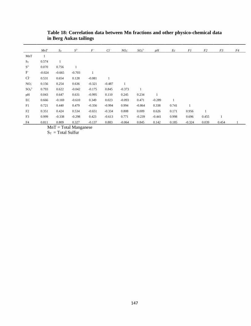
147
Table 18: Correlation data between Mn fractions and other physico-chemical data
in Berg Aukas tailings
MnT ST S2- F - Cl -
NO3- SO4
2- pH Ec F1 F2 F3 F4
MnT 1
ST 0.574 1
S2- 0.070 0.756 1
F- -0.024 -0.665 -0.703 1
Cl- 0.531 0.654 0.128 -0.081 1
NO3- 0.156 0.254 0.636 -0.321 -0.487 1
SO42- 0.793 0.622 -0.042 -0.175 0.845 -0.373 1
pH 0.043 0.647 0.631 -0.995 0.110 0.245 0.234 1
EC 0.666 -0.169 -0.610 0.349 0.023 -0.093 0.471 -0.289 1
F1 0.721 0.440 0.479 -0.356 -0.994 0.994 -0.864 0.338 0.741 1
F2 0.351 0.424 0.534 -0.651 -0.334 0.808 0.009 0.626 0.171 0.956 1
F3 0.999 -0.338 -0.298 0.423 -0.613 0.771 -0.239 -0.441 0.998 0.696 0.455 1
F4 0.811 0.809 0.327 -0.137 0.883 -0.064 0.845 0.142 0.185 -0.324 0.039 0.454 1
MnT = Total Manganese
ST = Total Sulfur