the open handbook of formal epistemology
TRANSCRIPT
T H E O P E N H A N D B O O K O F F O R M A L E P I S T E M O L O G Y
R ichard Pettigrew & Jonathan Weisberg , Eds .

T H E O P E N H A N D B O O K O F F O R M A LE P I S T E M O L O G Y
R ichard Pettigrew & Jonathan Weisberg , Eds .
Published open access by PhilPapers, 2019
All entries copyright © their respective authors and licensed under a CreativeCommons Attribution-NonCommercial-NoDerivatives 4.0 International License.

L I S T O F C O N T R I B U T O R S
R. A. BriggsStanford University
Michael CaieUniversity of Toronto
Kenny EaswaranTexas A&M University
Konstantin GeninUniversity of Toronto
Franz HuberUniversity of Toronto
Jason KonekUniversity of Bristol
Hanti LinUniversity of California, Davis
Anna MahtaniLondon School of Economics
Johanna ThomaLondon School of Economics
Michael G. TitelbaumUniversity of Wisconsin, Madison
Sylvia WenmackersKatholieke Universiteit Leuven
iii

For our teachers

Overall, and ultimately, mathematical methodsare necessary for philosophical progress. . .
— Hannes Leitgeb
There is no mathematical substitute for philosophy.— Saul Kripke
P R E FA C E
In formal epistemology, we use mathematical methods to explore thequestions of epistemology and rational choice. What can we know? Whatshould we believe and how strongly? How should we act based on ourbeliefs and values?
We begin by modelling phenomena like knowledge, belief, and desireusing mathematical machinery, just as a biologist might model the fluc-tuations of a pair of competing populations, or a physicist might modelthe turbulence of a fluid passing through a small aperture. Then, we ex-plore, discover, and justify the laws governing those phenomena, usingthe precision that mathematical machinery affords.
For example, we might represent a person by the strengths of theirbeliefs, and we might measure these using real numbers, which we callcredences. Having done this, we might ask what the norms are that governthat person when we represent them in that way. How should thosecredences hang together? How should the credences change in responseto evidence? And how should those credences guide the person’s actions?This is the approach of the first six chapters of this handbook.
In the second half, we consider different representations—the set ofpropositions a person believes; their ranking of propositions by theirplausibility. And in each case we ask again what the norms are that governa person so represented. Or, we might represent them as having bothcredences and full beliefs, and then ask how those two representationsshould interact with one another.
This handbook is incomplete, as such ventures often are. Formal epis-temology is a much wider topic than we present here. One omission, forinstance, is social epistemology, where we consider not only individualbelievers but also the epistemic aspects of their place in a social world.Michael Caie’s entry on doxastic logic touches on one part of this topic,but there is much more. Relatedly, there is no entry on epistemic logic, norany on knowledge more generally. There are still more gaps.
These omissions should not be taken as ideological choices. This materialis missing, not because it is any less valuable or interesting, but because we
v

failed to secure it in time. Rather than delay publication further, we choseto go ahead with what is already a substantial collection. We anticipate afurther volume in the future that will cover more ground.
Why an open access handbook on this topic? A number of reasons. Thetopics covered here are large and complex and need the space allowedby the sort of 50 page treatment that many of the authors give. We alsowanted to show that, using free and open software, one can overcome amajor hurdle facing open access publishing, even on topics with complextypesetting needs. With the right software, one can produce attractive, clearpublications at reasonably low cost. Indeed this handbook was created ona budget of exactly £0 (≈ $0).
Our thanks to PhilPapers for serving as publisher, and to the authors:we are enormously grateful for the effort they put into their entries.
R. P. & J. W.
vi

C O N T E N T S
1 precise credences 1
Michael G. Titelbaum2 decision theory 57
Johanna Thoma3 imprecise probabilities 107
Anna Mahtani4 conditional probabilities 131
Kenny Easwaran5 infinitesimal probabilities 199
Sylvia Wenmackers6 comparative probabilities 267
Jason Konek7 belief revision theory 349
Hanti Lin8 ranking theory 397
Franz Huber9 full & partial belief 437
Konstantin Genin10 doxastic logic 499
Michael Caie11 conditionals 543
R. A. Briggs
vii

1P R E C I S E C R E D E N C E S Michael G. Titelbaum
I am more confident than not that I will go in to my office tomorrow. I’mnot certain that I will go, and I haven’t even hit the point of believing thatI will: it is the summer, I have no courses to teach or students to meet,I may wake up tomorrow and decide it’s not worth the effort. But I’mmore confident that I will go than I am that I won’t. If I had to place myconfidence on a scale of 0 to 100, I’d put it somewhere above 50.
Credences are numerical degrees of confidence. While they could beexpressed as percentages—between 0 to 100, inclusive—it has becomecustomary to measure them on a scale from 0 to 1. Credences are also oftencalled “degrees of belief,” though that name may hold the connotationthat they are a species of ordinary, qualitative belief.
It’s better to think of credence not as a kind of qualitative belief, but in-stead as a member of the same family as qualitative belief. That family—thefamily of doxastic attitudes—also includes certainty, disbelief, suspensionof belief, and probably comparative confidence as well. The membersof this family have a variety of commonalities. For example, we tend tothink of credences as taking the same sorts of objects as outright beliefs.Many authors take these objects to be propositions, and so classify bothcredences and beliefs as propositional attitudes. I will follow that trendhere, but if you think beliefs are adopted towards something other thanpropositions (sentences, perhaps?), you will be inclined to the same viewabout credences.
The theory of credences was developed to address a number of philo-sophical problems. One was the proper interpretation of “probability”locutions. If I say, “The probability that I’ll go to the office tomorrow isover 50%,” what does this mean, and what are the truth-conditions for myutterance? A number of interpretations of probability have been offeredand defended (some of which we will discuss in Section 1.6), and it’s notclear that every use of the term “probability” should be interpreted thesame way. But one prominent suggestion, the “subjective interpretation ofprobability,” is that probability statements express the speaker’s degree ofconfidence in a proposition. So my utterance expresses a confidence over0.5 that I shall go to the office.
Yet even if “probability” statements rarely—or never—express an agent’sdegrees of confidence, such degrees of confidence may still exist, and havephilosophical work to do. Degrees of belief play a prominent role intraditional decision theory, the classic formal approach to rational choice
1

2 michael g . titelbaum
(about which more in Section 2.2). Credences also figure in Bayesianconfirmation theory (Section 2.1), an account of evidential support rivalingother statistical approaches such as frequentism and likelihoodism. Andthey can be applied to such further topics as coherentism, Inference to theBest Explanation, and social epistemology (Section 2.3).
So if we grant that credences exist, what exactly does it take to possessone? In line with contemporary behaviorist approaches in psychology, deFinetti (1937/1964) defined the degree of belief assigned to an event byan individual as the rate at which she’d bet that it would occur (moreabout the details in Section 2.2). But as was typical with operationalism,this definition ran into problems when, say, an agent displayed inconstantbetting behaviors over time, and so was difficult to assign a particular cre-dence to. Nowadays we may grant than an agent with a particular degreeof belief will, if rational, display particular betting behavior (Christensen,2004). But we also tend to think of this normative connection less as adefinition of credence and more as one aspect of what it is to possess a de-gree of confidence. Just as our account of qualitative belief has progressedbeyond behaviorism to a broader functionalism, we think of credence as amulti-faceted mental state with descriptive and normative connections toa wide variety of behaviors and other attitudes.
Besides their connections to desires, intentions, and decisions contem-plated in action theory and decision theory, credences are connected toother varieties of doxastic attitudes (not to mention emotions, sensations,and memories). If comparative confidence is a distinct type of mental state,it clearly is connected to credence: I am more confident of P than Q just incase my credence in P is higher than my credence in Q. As for qualitativeattitudes, certainty is often identified with credence 1 in a proposition(though see Section 1.7 below). There must also be links between credenceand outright belief: if I believe P, my credence in P should be higher thanmy credence in ∼P.
Can we find a fully general connection between credence and outrightbelief? Some authors (e.g., Holton, 2014) maintain that to the extent thereare any credences, to possess credence x in P is just to hold an outrightbelief that the probability of P is x. Yet it’s difficult to find a single conceptof probability that applies to every proposition to which an agent mightassign a degree of belief. And it seems agents (such as children) can bemore or less confident of propositions without possessing a concept ofprobability. Moreover, whatever concept of probability we select, it seemsconceivable for an agent to adopt a degree of confidence in the propositionthat P has probability x. (We’ll see a further technical difficulty withthe credence-as-outright-belief theory in Section 1.2.) Most theorists nowhold that the numerical value of a credence is an attribute of the attitude

precise credences 3
adopted towards a proposition, not part of the content of the propositiontowards which that attitude is adopted.1
Going in the other direction, the “Lockean Thesis”2 takes outright beliefjust to be credence above a particular threshold. The threshold credence isusually lower than 1 (belief need not be certainty) but well above 1/2, andmay depend on contextual parameters. The main objection to the LockeanThesis is that one can describe rationally acceptable credence distributionswhich, by way of the thesis, generate rationally unacceptable patterns ofbelief. In the Lottery Paradox (Kyburg, 1961) an agent assigns to eachticket in a lottery a low credence that it will win, while assigning a highcredence (perhaps certainty) that some ticket will win. For any Lockeanthreshold less than 1, we can arrange the numbers so that the agent windsup believing of each ticket that it will lose, while believing that some ticketwill win—a logically inconsistent overall set of beliefs. Similarly, in thePreface Paradox (Makinson, 1965), an author has high confidence in eachclaim made in her book while also being confident that at least one ofthose claims is false. Via the Lockean Thesis this becomes belief in eachconjunct of a conjunction coupled with disbelief in that conjunction.
How, then, to relate credence and outright belief in general? The mostradical possibility is to deny either the existence of beliefs or the existenceof credences. More conservatively, one could offer a reduction of onecategory to the other, or at least a principle of descriptive supervenience.Alternatively, one could grant that while beliefs and credences appear in avariety of configurations in actual agents, normative principles specify howthey’d align in a rational agent. The current consensus is that somethingbeyond just the Lockean Thesis would be required to make either of theseapproaches work; recent attempts to articulate belief-credence principlescan be found in Leitgeb (2017), Douven (2012), and Lin and Kelly (2012).
On the other hand, one could concede that beliefs and credences areboth genuine kinds of mental states an agent can possess, there are someways in which they interact (or interact if one is rational), but no systematicgeneral principles are available. While this stance is available to strongrealists about beliefs and credences, it is especially attractive to theoristswho read belief and credence ascriptions as convenient, simplifying modelsof a highly complex cognitive system. The belief-model and the credence-model are each effective and efficient in different circumstances, and maybe applied toward different ends. In that case, it would be unsurprising ifno universal translation from one to the other were available.
1 Moss (2018) takes the numerical value to be part of a credence’s content, but takes credalobjects to be more complicated than simple propositions.
2 Locke (1689/1975, Bk. IV). See also Foley (1993) for discussion.

4 michael g . titelbaum
1 rational constraints on credence
Once we understand what a credence is, the next question is what it takesfor a set of credences to be rational.
1.1 The Probability Axioms
The most generally-accepted rational credence norms are Kolmogorov’s(1933/1950) axioms. Suppose we have a language L of propositions, whichstarts with a finite set of atomic propositions and then closes them underthe standard truth-functional connectives. Define a real-valued function cover L representing the credence values an agent assigns the propositionsin L.3 The precise, real-number values that c assigns each proposition arethe “precise credences” of this entry’s title; I’ll discuss alternative formalapproaches in Section 5 below.
Given this setup, Kolmogorov’s axioms become the following.
Non-Negativity. For any X ∈ L, c(X) ≥ 0.
Normality. For any tautology T ∈ L, c(T) = 1.
Finite Additivity. For any mutually exclusive X, Y ∈ L,c(X ∨Y) = c(X) + c(Y).
Mathematicians often call these the probability axioms, and call any distribu-tion satisfying them a probability function. Probabilism is the position thatrational credences form a probability function; in other words, rationalcredences satisfy the Kolmogorov axioms.4
The probability axioms set 0 ≤ c(X) ≤ 1 for every X ∈ L. Probabilismalso entails a number of intuitive constraints on rational credence. Here’sone example.
For any X ∈ L, c(∼X) = 1− c(X).
Suppose you assign a high confidence that anthropogenic global warminghas occurred. This constraint requires you to assign a low confidencethat no anthropogenic warming has occurred. And should you becomemore confident that anthropogenic warming has occurred, this constraint
3 While I will consider languages containing propositions, other authors describe credencesas distributed over sentences, or sets of possible worlds, or sets of events, etc.
4 Probabilism is often described as the doctrine that rational agents have credences satisfyingthe probability axioms, or (if that’s considered too unrealistic) that ideally rational agentshave probabilistic credences. Both of these formulations make agents (real or ideal) thetargets of evaluation. Strictly speaking, I prefer to evaluate credences (or sets of credences)for rationality, rather than agents. But for ease of locution I will largely treat the two asinterchangeable here.

precise credences 5
will require your confidence in that proposition’s negation to decreaseaccordingly.
Some other intuitive constraints following from the Kolmogorov axioms.
For any contradiction F ∈ L, c(F) = 0.
For any X, Y ∈ L (mutually exclusive or otherwise),
c(X ∨Y) = c(X) + c(Y)− c(X & Y).
For any X, Y ∈ L, if X Y then c(Y) ≥ c(X).
For any logically equivalent X, Y ∈ L, c(X) = c(Y).
For any finite set of mutually exclusive X1, . . . , Xn ∈ L,
c(X1 ∨ . . . ∨ Xn) = c(X1) + . . . + c(Xn).
The last bulleted constraint has an important consequence when an agentconsiders a partition—a set of propositions whose members are mutuallyexclusive and jointly exhaustive. Because the disjunction of a partition’selements is a tautology, probabilism demands that the credences assignedto elements of a partition sum to 1.
A further important consequence of probabilism is that credences arestrongly extensional. If an agent is certain that two propositions X andY have the same truth-value (that is, if c(X ≡ Y) = 1), then for the sakeof calculating credences X and Y might as well be logically equivalent.For instance, any credence equation or inequality in which X appearswould remain true were any of its Xs replaced with Ys. Any difference inmeaning, modal profile, etc. is irrelevant to probability once truth-valuesare established to be identical.
We can illustrate probabilism with Kyburg’s Lottery example from page3. Given a lottery with, say, 100 tickets, introduce a language whose atomicpropositions are W1 through W100 (with Wi indicating that ticket i wins thelottery). If the lottery is fair, an agent might assign c(Wi) = 1/100 for eachWi. From our first intuitive consequence of the probability axioms, we thenhave c(∼Wi) = 99/100; the agent is highly confident of each ticket that itwill not win. However, assuming no more than one ticket can win, ourfinal intuitive consequence listed above yields:
c(W1 ∨ . . . ∨W100) = c(W1) + . . . + c(W100) = 1. (1)
So our agent is certain some ticket will win, as intuitively she ought tobe.5
5 Notice that none of this solves the Lottery Paradox, which brings full beliefs into the lotterypicture. My goal is just to illustrate how probabilism is compatible with and supportive ofa natural account of rational credences in the lottery case. A similar illustration could begiven for Makinson’s Preface example.

6 michael g . titelbaum
While proofs in the probability calculus usually proceed from Kol-mogorov’s axioms, practical problem-solving is often made easier by work-ing with state-descriptions. Define a literal to be an atomic propositionof L or its negation, then define a state-description in L to be a maximalconsistent conjunction of its literals. Every noncontradictory X ∈ L thenhas a unique disjunctive normal form, a disjunction of state-descriptionslogically equivalent to X.6
Carnap (1950) makes repeated use of the fact that a distribution cover L satisfies the probability axioms just in case it assigns: (1) non-negative values to L’s state-descriptions summing to 1; (2) for everynoncontradictory X, a value equal to the sum of the values assigned to thestate-descriptions in X’s disjunctive normal form; and (3) a value of 0 toevery contradictory proposition.7
This result is handy in two ways. First, we can completely characterizeany probability distribution over L by specifying the values it assigns to L’sstate-descriptions. Second, given partial information about a probabilitydistribution, we can determine what this information says about the valuesassigned to state-descriptions, then from there work out the values of (orconstraints on the values of) other propositions.
For example, suppose I tell you that Bob is certain of P ⊃ Q, and is twiceas confident of P as ∼P. It immediately follows that Bob’s confidence in∼Q is less than or equal to 1/3. Why? Well, the disjunctive normal formequivalent of ∼Q is (P &∼Q)∨ (∼P &∼Q). Since Bob is certain of P ⊃ Q,the first disjunct receives credence 0, so for Bob c(∼Q) = c(∼P &∼Q).But since c(P) + c(∼P) = 1, and c(P) = 2 · c(∼P), we have c(∼P) = 1/3.The disjunctive normal form equivalent of ∼P is (∼P & Q) ∨ (∼P &∼Q).By Non-Negativity Bob’s credence in the first disjunct must be greaterthan or equal to 0, so the second disjunct receives a credence less than orequal to 1/3.8
Finally, with the notion of a probability function in hand we can definethe notion of an expectation. Suppose we have a numerical quantity forwhich many values are possible. To calculate an agent’s expectation forthat quantity, we multiply each value times the agent’s credence that thequantity will take that value, then sum over all the values available. Forexample, if I’m 10% confident that I’ll go into my office two days this
6 To make the disjunctive normal form unique, we require literals to appear in a state-description in some canonical order (perhaps alphabetical, if the propositions are desig-nated by letters), and then we require state-descriptions to appear in disjunctive normalforms in a canonical order as well.
7 I have never been able to discover whether this result was original to Carnap or not. Iwould sincerely welcome any e-mails demonstrating its historical provenance!
8 For more on the mathematical theory underlying this approach, and for a Mathematicaroutine that will solve many probability problems once they are reduced to algebra usingstate-descriptions, see Fitelson (2008).

precise credences 7
week, 60% confident that I’ll go in just one day, and 30% confident that Iwon’t go in at all, then my expectation for the numbers of days I’ll go intomy office this week is:
0.10 · 2 days + 0.60 · 1 day + 0.30 · 0 days = 0.8 days. (2)
1.2 The Ratio Formula
So far we have discussed unconditional credence—an agent’s degree ofconfidence that a particular proposition is true in light of her currentunderstanding of what the world is like. We may also inquire after anagent’s conditional credence in proposition X given Y; this is the agent’scredence in X upon making the additional assumption that Y. Notice thatY may be a proposition in which the agent currently has low unconditionalcredence. In asking for her credence in X given Y, we ask her to set asideher current actual opinion about Y, temporarily add Y to the stock ofpropositions she takes to be true, then assess X in light of this enhancedsuppositional set.9
An agent’s conditional credence in X given Y is denoted c(X |Y), andis usually taken to be governed by the Ratio Formula.
Ratio Formula. For any X, Y ∈ L with c(Y) > 0,
c(X |Y) = c(X & Y)c(Y)
.
The Ratio Formula can be read as either a descriptive truth or as a norma-tive requirement. On the former approach, an agent’s conditional credenceX given Y takes a particular value just in case her unconditional credencesin X & Y and Y stand in that ratio. This reading is most natural if one wantsto reduce one type of credence to the other: one could hold that to have aconditional credence just is to have unconditional credences standing in aparticular ratio; or one could hold that conditional credences are basic andunconditional credences are a proper subset of those.10 Alternatively, onecould see conditional credence as just another type of doxastic attitude onequal footing with unconditional credences, then read the Ratio Formula
9 Notice that we are discussing indicative, not subjunctive, conditional credences. Thesupposition Y is to be added to the agent’s current set of assumptions about the world, withthe resulting suppositional set assumed to be consistent. Most discussions of conditionalcredence concern the indicative form. For a treatment of subjunctive conditional credences,see Joyce (1999).
10 From the Kolmogorov axioms and Ratio Formula, it follows that for any X ∈ L, c(X) =c(X |T). So unconditional credences can be thought of as conditional credences conditionalon a tautology. See Easwaran (this volume) for more.

8 michael g . titelbaum
as a rational requirement on how conditional and unconditional credencesshould align.11
Note that as I’ve defined the Ratio Formula, it remains silent when theagent assigns the condition (proposition Y) a credence of 0. We will returnto credences conditional on credence-0 propositions in Section 1.7.
Combining the Ratio Formula and Kolmogorov’s Axioms yields thehandy Law of Total Probability.
Law of Total Probability. For any X, Y1, . . . , Yn ∈ L such that theY1, . . . , Yn form a finite partition,
c(X) = c(X |Y1) · c(Y1) + . . . + c(X |Yn) · c(Yn).
The Law of Total Probability calculates the unconditional credence of Xas a weighted average of X’s credences conditional on members of theY-partition, weighted by the unconditional credences in the Ys.12
To illustrate once more with our lottery scenario, suppose B is theproposition that our agent will benefit from the outcome of the lottery. Sheholds tickets 1 through 3, so is sure to benefit if they win. Also, her sisterholds the very last ticket (ticket 100), and the agent is 1/2 confident thather sister will share the winnings should that ticket come in. Applyingthe Law of Total Probability (and recalling that Wi is the proposition thatticket i will win), the agent’s credence that she will benefit is
c(B) = c(B |W1) · c(W1) + c(B |W2) · c(W2) + c(B |W3) · c(W3)
+ c(B |W4) · c(W4) + . . . + c(B |W100) · c(W100)
= 1 · 1/100 + 1 · 1/100 + 1 · 1/100
+ 0 · 1/100 + . . . + 1/2 · 1/100
= 0.035.
(3)
Conditional credence also plays a crucial role in the notion of credalrelevance. When 0 < c(Y) < 1, all of the following inequalities are equiva-lent:
c(X |Y) > c(X), (4)
c(X) > c(X | ∼Y), (5)
c(Y | X) > c(Y), (6)
c(Y) > c(Y | ∼X), (7)
c(X & Y) > c(X) · c(Y). (8)
11 For a discussion of how conditional credences interact with an agent’s credences inconditionals, see Briggs (this volume).
12 Put another way, the Law of Total Probability requires an agent’s unconditional credencein X to equal her expectation of her credence in X conditional on the true element of theY-partition.

precise credences 9
When these inequalities hold, we say that Y is positively relevant to Xon the agent’s credence function. (Since positive relevance is a symmetricrelation, we may also say that X is positively relevant to Y.) Another wayto put this is that the agent takes X and Y to be positively correlated.Replacing the greater-thans with less-thans describes when Y is negativelyrelevant to X (or negatively correlated with X) on an agent’s credences.On the other hand, when c(X & Y) = c(X) · c(Y) (or any of the otherinequalities above becomes equality), we say that X is irrelevant to Y forthe agent, or probabilistically independent of Y.
These relevance relations are relative to an agent’s credences; they reflectwhich propositions she assesses as relevant to each other given her currentunderstanding of the world. But we can also temporarily enhance hercurrent set of suppositions about the world, and see whether any relevancerelations change. This takes us from a notion of unconditional relevanceto conditional relevance. Y is relevant to X conditional on Z just in case
c(X |Y & Z) > c(X | Z). (9)
For each of the inequalities above, a corresponding characterization ofconditional relevance can be given by adding Z as a condition to theexpressions on each side.
The notion of conditional relevance underlies a crucial notion in thephilosophy of science: screening off. We say that Z screens off X fromY when X and Y are unconditionally dependent but the following twoequalities hold:
c(X |Y & Z) = c(X | Z), (10)
c(X |Y &∼Z) = c(X | ∼Z). (11)
In other words, X and Y are independent conditional on each of Z and∼Z. In a screening-off situation, supposing either Z or ∼Z makes thecorrelation between X and Y disappear.13
To illustrate one application of this concept, Reichenbach (1956) arguesthat a common cause screens off its effects from each other. Suppose X isthe proposition that my newspaper reports that the Yankees won last night,Y is the proposition that your newspaper reports that the Yankees wonlast night, and Z is the proposition that the Yankees actually won. On theone hand, while I remain ignorant of Z it would be rational for me to treatX as relevant to Y. X provides information about Z, and therefore alsoprovides information about Y. But once the truth-value of Z is established,X and Y lose the ability to say anything about each other; X and Y become
13 This definition generalizes to the case in which Z is a random variable capable of taking avariety of values zi. Screening off then occurs when X and Y are unconditionally correlated,but become independent conditional on each proposition of the form Z = zi.

10 michael g . titelbaum
independent conditional on any supposition about Z. Thus Z will screenoff X from Y on my credence function.
A proximal cause will also screen off its effect from a distal cause. (Imag-ine Y states the final score of last night’s Yankees game, Z is the propositionthat the Yankees won, and X is the proposition that my newspaper reportsthat they won.) In general, probabilistic correlations (conditional and un-conditional) can provide useful evidence about the causal relations amonga set of variables. Some philosophers have even defined causality in termsof probabilistic relations. For more on all of this, see Hitchcock (2012).
One final point about conditional credences. Earlier (p. 2) I mentionedthe theory that a credence of x in P is just the outright belief that theprobability of P is x. There I noted a number of problems for that theory;now we can add that the theory seems to lack a good way of understandingconditional credence. A conditional credence c(P |Q) of x cannot be readas a qualitative belief in the proposition “If Q, then the probability of P isx,” nor can it be read as the belief that “The probability of ‘If Q, then P’ isx.” This was established by a series of triviality results initiated by Lewis(1976).14 For instance, Lewis’ work shows that if we assume c(P |Q) = xjust in case p(Q→ P) = x for some suitable notion of probability p andsome indicative conditional →, then it follows that every proposition isprobabilistically independent from every other! This is obviously absurd. Aconditional credence just isn’t a credence—or a belief—about a conditional.
1.3 Updating by Conditionalization
The rational constraints on credence listed to this point have beensynchronic—when they relate multiple credences, all the credences relatedare held at the same time. The degree of belief literature has also proposeda number of diachronic constraints, governing relations among credencesassigned at different times.
Suppose we have two times, ti and tj, with the latter occurring after theformer. Let ci and cj be the agent’s credence functions at these two times.The most traditional, well-established, and well-known diachronic credalconstraint is Conditionalization.
Conditionalization. If E ∈ L represents everything the agent learnsbetween ti and tj, then for any X ∈ L, cj(X) = ci(X | E).
The intuitive idea of Conditionalization is simple. Suppose that at ti youdon’t know whether E is true. I ask you to hypothetically suppose E(temporarily add it to your stock of assumptions about what the world islike), then ask for your conditional credence in X given this supposition.
14 For the recent state of the art in this area, see Hájek (2011) and Fitelson (2015).

precise credences 11
You offer some number. Then, between ti and tj, you learn that E isactually true (and learn nothing else besides). If I now ask you at tj foryour unconditional credence in X, it seems you should offer the samenumber you reported as a conditional credence before. After all, the set ofreal-world conditions against which you’re assessing X is the same at bothtimes; it’s just that at ti you were supposing E as a fact about the world,while at tj you know E to be true.
Conditionalization integrates nicely with our other credal constraints.For instance, if ci satisfies the Kolmogorov axioms and ci(E) > 0, thenconditionalizing yields a cj distribution that satisfies the axioms as well. Soif an agent begins with a probability distribution and repeatedly updatesby conditionalizing, she is guaranteed to respect probabilism on an ongo-ing basis. The probability axioms and Ratio Formula also make updatingby conditionalization cumulative and commutative. If you conditionalizesuccessively on E and then E′, this yields the same result as conditional-izing just once on E & E′, which means it also yields the same result asconditionalizing on E′ followed by E.
For a conditionalizing agent, current credences interact in an interestingway with predictions about future credences. Suppose an agent is certain atti that her tj credences will be formed by conditionalizing on a propositionshe will learn from some particular finite partition. (Perhaps she willconduct an experiment between ti and tj, and the propositions in thepartition represent all of its possible outcomes.) Assuming she meets a fewother plausible side-conditions, such an agent will satisfy the ReflectionPrinciple.
Reflection Principle. For any X ∈ L, ci(X | cj(X) = r) = r.
This principle, introduced by van Fraassen (1984), sets the agent’s ti un-conditional credence in X equal to her ti expectation of her unconditionaltj credence in X.15 Notice that although a cj appears in the righthandexpression, the principle governs synchronic credal interactions: it relatesthe agent’s ci credences in X to her ci credences about her future credencesin X. Given (again) a few side-conditions, Reflection may be derived fromthe Kolmogorov axioms, the Ratio Formula, and the agent’s certainty thatshe will update by conditionalizing on some member of a particular parti-tion. Van Fraassen, however, argues in the opposite direction: he providesindependent motivation for Reflection, then views Conditionalization asa derivable consequence. For more on the arguments in each direction,and the specific side-conditions required, see Weisberg (2007) and Briggs(2009).
15 To see why, return to our formulation of the Law of Total Probability on page 8, andlet each Yi there assert that the agent’s unconditional tj credence in X will take someparticular real value r.

12 michael g . titelbaum
When an agent repeatedly updates by Conditionalization, she oftenfinds herself calculating the value of c(X | E). This calculation can bestreamlined by a famous theorem.
Bayes’ Theorem. For any X, E ∈ L with non-zero c-values,
c(X | E) = c(E | X) · c(X)
c(E).
Bayes’ Theorem has proved so central to the application of Conditional-ization that theorists who work with degrees of belief are often called“Bayesians” (or “subjective Bayesians,” or “Bayesian epistemologists”). In amoment I’ll describe why Bayes’ Theorem is so useful. But first, it’s worthnoting that Bayes’ Theorem is indeed a theorem, easily derivable from theKolmogorov Axioms and Ratio Formula.16 Bayesianism has generated agreat deal of controversy, especially among statisticians. But the contro-versial claim in Bayesianism isn’t that Bayes’ Theorem is true. Everyoneagrees that the theorem follows from the Kolmogorov Axioms, and that ifan agent is going to generate new credences over time by conditionaliz-ing, then the theorem provides a handy tool for calculating post-updatecredences from pre-update credences. The controversy is whether agentsshould really update their credences by conditionalizing, and whetherscientific inference is best understood as a series of conditionalizations.
Setting this controversy aside, why is the particular analysis of c(X | E)in Bayes’ Theorem so useful? Consider a scientific context, in which atheorist has a finite partition of hypotheses H1, . . . , Hn about what’s goingon with some phenomenon. The theorist plans to run an experiment thatshe hopes will discriminate among the hypotheses. At time ti, before shehas run the experiment, the theorist has a set of unconditional credences ci,which we call her priors. The theorist runs the experiment between ti and tj,and let’s suppose the observation she makes is represented by propositionE. Given this new evidence, Conditionalization helps her calculate hercredences at tj, which we call her posteriors.
Suppose we’re interested in the theorist’s confidence in some particularhypothesis Hm after the experimental results come in. Applying Condi-tionalization, Bayes’ Theorem, and then the Law of Total Probability to thedenominator of Bayes’ Theorem, we derive:
cj(Hm) =ci(E | Hm) · ci(Hm)
ci(E | H1) · ci(H1) + . . . + ci(E | Hn) · ci(Hn). (12)
16 The theorem is traditionally attributed to the Reverend Thomas Bayes. Though Bayes neverpublished the theorem, Richard Price found it in his notes and published it after Bayes’death in 1761. Pierre-Simon Laplace rediscovered the theorem independently later on, andwas responsible for much of its early popularization.

precise credences 13
Consider the components of the right-hand fraction one at a time. First, wehave a number of expressions of the form ci(Hx). These are the theorist’spriors in the various hypotheses. Presumably going into the experimentshe has some unconditional levels of confidence in the hypotheses she isconsidering; these supply the priors in question. Then we have expressionsof the form ci(E | Hx). An agent’s conditional credence in an experimentalresult E given some hypothesis Hx is called her likelihood for that evidenceon that hypothesis. A well-defined scientific hypothesis should make aprediction for how the theorist’s experiment will come out, or at leastshould assign probabilities to various possible outcomes. These informthe theorist’s likelihoods for various experimental outcomes (such as E)on the various hypotheses she entertains. Thus Bayes’ Theorem allows thetheorist to form a posterior opinion about each hypothesis Hm that sheentertains, based on the evidence she’s received, her unconditional priorsin the hypotheses, and her ti likelihoods—elements that are plausibly alleasily to hand.
1.4 Jeffrey Conditionalization
Statisticians and philosophers of science often worry that Conditional-ization allows a scientist’s final verdict on a hypothesis to be influencedby her initial credence in that hypothesis—her personal degree of beliefin the hypothesis before any evidence came in. Epistemologists worryabout Conditionalization’s conception of evidence. It seems that for Con-ditionalization to work, it must be possible to identify some propositionE representing everything the agent learns between ti and tj. Moreover,the agent must become certain of E between ti and tj, because updatingthe agent’s credence in E itself using Conditionalization yields cj(E) = 1.Finally, once an agent becomes certain of some proposition, subsequentupdates by Conditionalization will retain that certainty forever.17
Conditionalization therefore seems to embody a conception of learningon which what is learned is explicitly summarizable in propositional form,becomes certain, and is retained ever after. To epistemologists, this isreminiscent of foundationalist approaches to evidence abandoned decadesago. It also violates the Regularity Principle, which deems it irrational foran agent to assign absolute certainty to an empirical proposition. (Afterall, what evidence could ever make you entirely certain that some empiricalclaim was true?)
To address these problems, Richard C. Jeffrey offers an updating rulethat generalizes Conditionalization to allow for learning experiences in
17 It’s easy to show that if an agent conditionalizes on E between ti and tj, she will havecj(E) = 1, and then if she conditionalizes on some other evidence between tj and tk, shewill still have ck(E) = 1 as well.

14 michael g . titelbaum
which no certainties are gained. He introduces his rule using the followingexample.
The agent inspects a piece of cloth by candlelight, and gets theimpression that it is green, although he concedes that it mightbe blue or even (but very improbably) violet. If G, B, and Vare the propositions that the cloth is green, blue, and violet,respectively, then the outcome of the observation might be that,whereas originally his degrees of belief in G, B, and V were .30,.30, and .40, his degrees of belief in those same propositionsafter the observation are .70, .25, and .05. (Jeffrey, 1965, p. 154)
Discussing the example, Jeffrey writes:
If there were a proposition E in [the agent’s] preference rankingwhich described the precise quality of his visual experience inlooking at the cloth, one would say that what the agent hadlearned from the observation was that E is true. . . . But thereneed be no such proposition E in his preference ranking; norneed any such proposition be expressible in the English lan-guage. . . . The description ‘The cloth looked green or possiblyblue or conceivably violet,’ would be too vague to convey theprecise quality of the experience. . . . It seems that the best wecan do is to describe, not the quality of the visual experienceitself, but rather its effects on the observer, by saying, “Afterthe observation, the agent’s degrees of belief in G, B, and Vwere .70, .25, and .05.” (Jeffrey, 1965, pp. 154–5)
Jeffrey proposed an updating rule he called “probability kinematics”;nowadays everyone calls it “Jeffrey Conditionalization.” The rule applieswhen an agent’s experience impinges on her credences by altering herdegree of belief distribution across a particular finite partition in L; anyother changes in her credences are caused by the changes to this partition.If the originating partition is B1, . . . , Bn, then Jeffrey’s rule is as follows.
Jeffrey Conditionalization. For any A ∈ L,
cj(A) = ci(A | B1) · cj(B1) + . . . + ci(A | Bn) · cj(Bn).
Jeffrey did not mean to rule out the possibility that some learning occursby certainty acquisition. He just wanted to allow for the possibility ofother types of learning experiences as well. So in the case where one ofthe Bm goes to certainty (and therefore every other member of the parti-tion goes to credence-0), Jeffrey Conditionalization reduces to traditionalConditionalization.

precise credences 15
Let’s see how Jeffrey Conditionalization applies to Jeffrey’s cloth bycandlelight example. Suppose the agent is interested in the propositionM, that the selected piece of cloth will match her couch. She’s certainthat anything violet will match, she’s certain anything green will not, andshe’s 50% confident that a blue cloth will match. (The match dependson the specific shade of blue.) Let ti be the time before she inspects thecloth by candlelight. Using the Law of Total Probability and the initialunconditional credences Jeffrey provides, we have
ci(M) = ci(M | G) · ci(G) + ci(M | B) · ci(B) + ci(M |V) · ci(V)
= 0 · .30 + 0.5 · .30 + 1 · .40 = 0.55.(13)
Jeffrey also provides the agent’s unconditional credences in G, B, and V attj, after the inspection. With these values, Jeffrey Conditionalization yields
cj(M) = ci(M | G) · cj(G) + ci(M | B) · cj(B) + ci(M |V) · cj(V)
= 0 · .70 + 0.5 · .25 + 1 · .05 = 0.175.(14)
The glimpse by candlelight increases the agent’s confidence that the clothis green and decreases her confidence that the cloth is violet, so the Jeffrey-prescribed posterior that the cloth will match decreases.
Notice how this change in credence is effected. The agent’s visualexperience changes her credences by directly altering her distributionacross the cloth-color partition. Any changes to other propositions inthe agent’s language (such as M) are downstream effects of this directalteration. Yet the dependencies between these downstream propositionsand the color propositions remain unaltered: changing the agent’s opinionsabout the color of the cloth doesn’t change how confident she is thatparticular colors will match the couch. This is why the same conditionalcredences appear in both the ci(M) and the cj(M) calculations.
Against the background of the Kolmogorov axioms and Ratio Formula,Jeffrey Conditionalization is equivalent to the following condition.
Rigidity. For any A ∈ L and any Bm, cj(A | Bm) = ci(A | Bm).
In a Jeffrey Conditionalization, experience alters an agent’s credencesacross the B-partition. The agent’s credences in other propositions con-ditional on the Bms don’t change. So the agent sets her posteriors byadopting unconditional credences in the Bms from experience, copyingover her old conditional credences, then applying the Law of Total Proba-bility to calculate her unconditional credences in non-B propositions.
1.5 Further Rational Requirements
We have now seen a variety of putative rational constraints on credence: theprobability axioms, the Ratio Formula, the Reflection Principle, Regularity,

16 michael g . titelbaum
and the diachronic rules of Conditionalization and Jeffrey Conditionaliza-tion. Yet there are infinitely many credence distributions (and sequencesof credence distributions over time) compatible with these constraints. Areall of those distributions rationally permissible? Some of them are quitestrange, and unintuitive—for instance, some assign very high credence toskeptical scenarios; some will lead agents to reason counter-inductively.
One extreme position about the strength of rational constraints is some-times called “Objective Bayesianism.” This position endorses the Unique-ness Thesis (Feldman, 2007; White, 2005) that given any body of evidence,there is exactly one credence distribution rationally permitted to any agentwith that body of total evidence. At the other extreme, what we mightcall “Extreme Subjective Bayesians” hold that any probabilistic credencedistribution is rationally permissible. In between are “Moderate SubjectiveBayesians,” who hold that there are some rational constraints beyond theones we’ve described, but not enough to generate a unique permissibledistribution in every case.
What might these further rational constraints be? A constraint thatmight considerably narrow the field of what’s rationally permissible is the
Principle of Indifference. If an agent has no evidence favoring anypossibility in a partition over any other, then she should assign equalcredence to each element of the partition.18
The traditional objection to this principle is that it seems to give conflictingadvice when we repartition the same space of possibilities. Following vanFraassen (1989), suppose I tell you that a cube has been produced from afactory, and its side length is between 0 and 1 meter. Given the paucity offurther evidence, if I ask how confident you are that the side length is lessthan 0.5 meters, the Principle of Indifference seems to require a credence of1/2. But if I now ask how confident you are that the volume (which mustbe between 0 and 1 cubic meter) is less than 0.5 cubic meters, the Principleof Indifference also seems to require a credence of 1/2. Since a side lengthof 0.5 meters corresponds to a volume of 0.125 cubic meters, the only wayto assign both these credences consistently with the probability axioms isto be absolutely certain that the volume in cubic meters is not between0.125 and 0.5!19
Another family of putative rational constraints has a member we’vealready seen. The Reflection Principle directs us to set our current uncon-
18 The basic idea here dates back at least to Laplace (1814/1995), who saw it as an applicationof what Bernoulli (1713) called the “principle of insufficient reason.”
19 A more technically-sophisticated cousin of the Principle of Indifference is Jaynes’ (1957a,1957b) Maximum Entropy Principle. This principle applies more naturally over infinitepartitions, and adapts well to a variety of forms of evidence. Yet it still succumbs topartition variance problems, and also conflicts with updating by conditionalization inparticular cases. See Seidenfeld (1986).

precise credences 17
ditional credence in a proposition equal to what we’re certain it will be inthe future—or if we’re not certain of our future credences, equal to ourexpectation of what they will be. This principle directs us to defer to theopinions of our future self as if she were some sort of expert. But of coursethere are other experts in the world, such as contemporaries who we thinkhave better judgment or information than ourselves. Following the leadof the Reflection Principle, Elga (2007) suggests that if ce is the credencedistribution of an agent we consider an expert, then for any X ∈ L (or atleast any X in the expert’s area of expertise) we should assign
c(X | ce(X) = r) = r. (15)
Thinking more metaphorically, an “expert” distribution worthy of ourdeference need not even be an agent. It may be rational to align ourcredences with certain objective numerical values in the universe. Thisbrings us to the topic of direct inference principles.
1.6 Direct Inference Principles
Page 1 briefly mentioned interpretations of probability—proposals for themeaning of “probability” locutions. For example, the classical interpreta-tion, dating back at least to Laplace (1814/1995), defined probability as thenumber of favorable outcomes of a process divided by the total number ofoutcomes possible. Later, the frequency theory of probability (associatedmost closely with von Mises, 1928/1957), read probability as the frequencywith which an outcome would occur were a particular process repeatedmany times.20
My task here is not to assess these notions of probability as proposals inthe theory of meaning, or in the theory of probability. Instead, I want toask what these notions have to do with rational credence. Many Bayesianshave endorsed principles of direct inference: principles carrying the agentfrom information about some notion of probability to specific credencesin specific events. For example, it might be that if I’m certain a particulartype of experimental setup produces a particular type of outcome withfrequency x, then when an experiment of that type is to be run, I shouldhave credence x that it will yield an outcome of that type. This would be aprinciple of direct inference from frequency facts to credences in outcomes.
Frequency-to-credence principles face notorious difficulties, even whensketched out as roughly as I’ve just done. For one, a single event (I go
20 The previous section introduced one usage of “Objective/Subjective Bayesian” terminology.That usage should be carefully distinguished from another usage that often comes up in theliterature about interpretations of probability. In that literature, “Subjective Bayesianism”describes the position that in everyday talk, “probability” always refers to or expressessubjective credences. “Objective Bayesianism,” on the other hand, holds that probabilitytalk refers to something beyond the subject, such as frequencies or chances.
18 michael g . titelbaum
in to my office tomorrow) can be classed as the outcome of a variety ofexperiment types (choosing whether to go in on a summer day, choosingwhether to go in on a Tuesday, etc.), which may yield different frequenciesand therefore different credal recommendations. (This is one version ofthe “reference class problem.”21) Also, if we tried to use this principle as ageneral credence-setting strategy, we’d have trouble with experiments thatlook to be unrepeatable. Before the Large Hadron Collider was switchedon, newspapers prominently reported physicists’ degrees of belief thatdoing so would destroy the Earth. It’s difficult to align such credenceswith the frequency with which switching on the collider would causeglobal destruction; in the event of such destruction, the switching-on onlyoccurs once.
It may therefore be preferable to link rational credence with “objectivechance.” As a notion of probability, chance is objective, in the sense that itsvalue is determined by the physical makeup of an experimental apparatus.Chance may also be applied to events that occur only once. A frequency-to-credence principle recommends credence 1/6 that a fair die roll willcome up 3 on the grounds that repeating the roll will yield 3 one-sixth ofthe time. The objective chance theorist recommends 1/6 on the groundsthat a fair die is physically constituted in a particular manner (equallyweighted on each side, etc.). This would remain true even if the die hadnever been rolled before, and was guaranteed to be destroyed after the rollin question.
The most famous direct inference principle linking credence and chanceis Lewis’ (1980) Principal Principle. Very roughly, and skipping over agreat many details,22 the Principal Principle directs an agent to set
c(A | Ch(A) = x) = x, (16)
unless she possesses inadmissible evidence relevant to A. Here Ch(A) = xis the proposition that the objective chance of A is x. So—setting asidethe matter of inadmissible evidence for a moment—if the agent is certainthat, say, a particular die has a 1/6 chance of coming up 3, the PrincipalPrinciple will set her credence in 3 at 1/6. If, on the other hand, the agentknows the die is biased, but splits her credence evenly between the number3’s having a 1/10 chance and a 1/5 chance of coming up, the Law of TotalProbability will combine with the Principal Principle to yield:
c(3) = c(Ch(3) = 1/10) · c(3 | Ch(3) = 1/10)
+ c(Ch(3) = 1/5) · c(3 | Ch(3) = 1/5)
= 1/2 · 1/10 + 1/2 · 1/5
= 0.15.
(17)
21 See Hájek (2007) for many more versions.22 See Meacham (2010) for some of those details.

precise credences 19
In other words, her credence that the die will come up 3 is her expectationof the objective chance of getting a 3. We can therefore think of the PrincipalPrinciple as an expert deference principle in which the expert is objectivechance.
The key innovation of Lewis’ Principal Principle is its treatment of ev-idence the agent takes to be relevant to the outcome of a chance event.Lewis divides such evidence into two sorts: admissible evidence is evi-dence that the agent takes to be relevant to the outcome because it affectsher opinion of the objective chance of the event. For example, informationabout the weighting of the die is admissible with respect to the outcomeof the roll—it affects how the agent thinks the roll will come out by wayof affecting what the agent thinks are the chances of a 3. Inadmissibleevidence affects the agent’s opinion in some other way. For instance, if aconfederate tells her how the roll came out, this affects the agent’s opinionof whether it came out 3, but not by making her think the chances of a 3were any different going in. Lewis’ insight was that chance facts about anoutcome screen off admissible information relevant to that outcome. So ifE is admissible, the Principal Principle also gives us:
c(A | Ch(A) = x & E) = c(A | Ch(A) = x) = x. (18)
Admissible evidence relates to chances much the way a distal cause relatesto the proximal cause of an event.
1.7 Countable Additivity
Up to this point the examples we’ve considered have typically involvedonly finitely many possibilities. But what if an agent considers a parti-tion of infinitely many possible outcomes, and distributes her credenceequally among all of them? How can this be modeled in our Bayesianepistemology?
To have a concrete example, let’s suppose that a positive integer has beenselected by some process, and our agent wants to assign equal credence toeach integer’s having been selected. Presumably that should be possible.But what numerical value might that credence take? It’s easy to show thatthe probability axioms prevent its being a positive real. For suppose theagent assigns
r = c(1) = c(2) = c(3) = . . . . (19)
(Where c(1) is her credence that 1 was selected.23) For any positive real r,there will exist a positive integer n such that r > 1/n. Now consider the
23 Notice we are now dealing with a language containing infinitely many atomic propositions.While this is a change from our earlier setup, it’s not too difficult to manage, and is fairlycommon in formal models.

20 michael g . titelbaum
agent’s credence that the selected integer is between 1 and n (inclusive).If you look back at the list of intuitive constraints following from theKolmogorov axioms (Section 1.1), the last principle on the bulleted listwill give us
c(1∨ 2∨ . . . ∨ n) = c(1) + c(2) + . . . + c(n) = r · n > 1, (20)
which violates the axioms.What other options are available? One popular suggestion is that when
an agent assigns equal confidence to infinitely many possibilities, werepresent that level of confidence as a credence of 0. So we would say thatc(1) = c(2) = . . . = 0.
Using credence 0 in this way introduces a few problems. First, upuntil this point we’ve conceived credence 1 as representing certainty in aproposition, and credence 0 as certainty that the proposition is false. Nowwe’ll have to allow an agent to assign c(P) = 0 even if the agent admitsP might be true, and c(∼P) = 1 even if the agent isn’t certain P is false.And we’ll have to phrase the Regularity principle carefully: we may stillprohibit agents from assigning certainty to empirical propositions, but nolonger ban credences of 1 and 0 in such propositions.
Second, the Ratio Formula we’ve provided only relates the conditionalcredence c(X |Y) to unconditional credences when c(Y) > 0. We’ll needto expand this principle to handle cases in which c(Y) = 0 yet the agentdoesn’t rule Y out. For instance, our agent assigning equal credence tothe selection of each positive integer might assign c(2 | 2∨ 4) = 1/2, eventhough c(2∨ 4) = c(2) + c(4) = 0.24
Third and most importantly, we’ll want a way to sum credences overinfinite disjunctions. Finite Additivity only covers disjunctions with finitelymany disjuncts—what if we want to calculate our agent’s credence thatthe selected integer is even? A natural extension of Finite Additivity is thefollowing.
Countable Additivity. For any countable partition Q1, Q2, Q3, . . . ⊂L,
c(Q1 ∨Q2 ∨Q3 ∨ . . .) = c(Q1) + c(Q2) + c(Q3) + . . . .
Countable Additivity is not only natural; it also allows us to establish avery important constraint on credences.
Conglomerability. For any proposition P ∈ L and partition Q1, Q2,Q3, . . . ⊂ L, c(P) is no greater than the largest c(P |Qi) and no lessthan the least c(P |Qi).
24 One way to manage this situation is to take conditional credences as basic. See footnote 10
for more information.

precise credences 21
Given Conglomerability, the c(P |Qi) establish upper and lower boundson the value of c(P). This makes sense if you think of c(P) as a weightedaverage of the credences the agent would assign to P conditional on allthe different possible Qi. And it’s especially important when the agent hasa partition E1, E2, E3, . . . of possible new pieces of evidence she mightreceive before her next update. Assuming she plans to update by Condi-tionalization, she knows that her future credence in P will be one of hercurrent c(P | Ei); Reflection then demands she satisfy Conglomerability.25
The Conglomerability/Countable Additivity package is attractive. Butit’s inconsistent with assigning a credence of 0 to each positive integer inour example. The reason is simple: given Countable Additivity, the agent’scredence that any positive integer will be selected at all is the sum of hercredences in each individual integer. But the former value should be 1,while the latter individual values are each 0. So advocates of CountableAdditivity have suggested instead that in this situation the agent assignan infinitesimal value to each integer’s being selected. The infinitesimalsare an extension of the set of real numbers, defined to be greater than0 but less than any given real number. Thus they don’t fall prey to theproblem of our Equation 20. At the same time, adding up infinitely manyinfinitesimals can yield a real number, so we can maintain both CountableAdditivity and a credence of 1 that any integer will be selected at all.
Yet infinitesimals introduce difficulties of their own; for some of thedifficulties, and many of the mathematical details, see Hájek (2003, Section5), Williamson (2007), Easwaran (2014), and Wenmackers (this volume).
2 applications of credence
I’ve presented the Bayesian study of credence as the study of a doxasticattitude type, and what it takes to make such attitudes rational. This studyis valuable in its own right, as a contribution to epistemology and thephilosophy of mind. But historically it’s also been pursued to enhance ourunderstanding of other topics, some of which we’ll discuss in this section.
2.1 Confirmation Theory
A Bayesian epistemologist or philosopher of science studies justificationand evidential support by thinking about “confirmation.” The type of con-
25 Notice that my statement of Conglomerability doesn’t specify the cardinality of theQi partition. For finite partitions, Conglomerability can be proven from the standardprobability axioms. Adopting Countable Additivity extends Conglomerability to countablepartitions. For an agent who entertains larger disjunctions than that, Seidenfeld, Schervish,and Kadane (manuscript) show that at each cardinality we need the relevant Additivityprinciple to secure Conglomerability for partitions of that size.

22 michael g . titelbaum
firmation studied is usually incremental, rather than all-things-considered;when we say that “evidence E confirms hypothesis H,” we mean that Eprovides at least some positive evidential support for H, not that it settlesthe matter of H or even pushes H past some crucial threshold.26 For aBayesian, confirmation is also always relative to a probability distribu-tion, and to a background corpus of propositions. Most commonly, theprobability distribution will be some agent’s credence function, and thebackground corpus will be the total evidence informing that credencefunction. (On a Conditionalization regime, the corpus is represented for-mally by the set of all propositions X such that c(X) = 1.27) So we take agiven agent at a given time, and ask whether E confirms H for her, relativeto her credences and background corpus at that time.
Letting K represent a background corpus, and ck represent a probabilitydistribution informed by that corpus, Bayesian confirmation theory positsthat
E confirms H relative to ck just in case ck(H | E) > ck(H).
Bayesian confirmation is just positive probabilistic relevance relative to ck.(Similarly, disconfirmation is usually defined as negative relevance relativeto ck.)
Though fairly simple, this theory of confirmation turns out to be surpris-ingly subtle, powerful, and convincing. To illustrate—and fix the intendednotion of evidential support in the reader’s mind—suppose a fair diehas just been tossed, and you know nothing of the outcome. Perhaps inaccordance with the Principal Principle, some frequency principle, or eventhe Principle of Indifference, you assign equal credence to each of the sixpossible outcomes. Relative to your credence distribution and backgroundcorpus, if you received evidence that the toss came up with a prime num-ber, this would confirm for you that the toss came up odd. Why? Becauseif you satisfy the Kolmogorov axioms and Ratio Formula, then you assign
2/3 = c(odd | prime) > c(odd) = 1/2. (21)
This doesn’t mean that prime evidence should make you certain the tosscame up odd, or even that it would justify you in believing the toss cameup odd. But if you update by Conditionalization, learning that the tosscame up prime would make you at least somewhat more confident thatthe toss came up odd. Again, the confirmation here is incremental.
26 This contrasts with the way “confirms” is sometimes used in English, as when we speakof a nominee’s being confirmed, or even a dinner reservation.
27 Notice that despite our suggestion in Section 1.7 that it might sometimes be interpretedotherwise, I have gone back to treating credence 1 as representing certainty. To simplifydiscussion, I will continue to do this going forward.
precise credences 23
This Bayesian theory of confirmation gives the confirmation relationsome interesting and intuitive formal properties.28
If E E′ and H H′, then E confirms H just in case E′ confirmsH′.
E confirms H just in case E disconfirms ∼H.
If E & K H but K 2 H, then E confirms H.
If H & K E but K 2 H, then E confirms H.
The first of these properties ensures that logical equivalents behave thesame within the confirmation relation. The second relates confirmation todisconfirmation. The third and fourth properties29 specify how confirma-tion relates to entailment. The third property tells us that entailment is aform of confirmation; if E entails H jointly with K while K didn’t entailH on its own, then E confirms H. As for the fourth property, it capturesthe idea30 that a hypothesis which predicts an evidential observation (inconcert with one’s background corpus) is confirmed by that observation.
On the other hand, the Bayesian theory withholds from the confirmationrelation certain properties that are sometimes mistakenly ascribed to it.Here are two examples.
If E confirms both H and H′, then the set H, H′, K is logically consis-tent.
If X confirms Y and Y confirms Z, then X confirms Z.
The first of these properties is important to reject because we’re talkingabout incremental confirmation. For example, in Jeffrey’s example in whichan agent inspects a piece of cloth by candlelight, his brief glimpse mayconfirm that the cloth is green, while also confirming that it’s blue oreven that it’s violet. (Perhaps the glimpse disconfirms that the cloth isred and disconfirms that it’s orange.) This is perfectly reasonable, despitethe fact that green, blue, and velvet are inconsistent hypotheses about thecolor of the cloth. Similarly, in scientific settings the same observation mayconfirm mutually exclusive theories from a partition, while at the sametime (perhaps) ruling others out.
The latter property is the supposed property of confirmation transitivity.This is one of the most common mistakes made about confirmation, sup-port, justification, and other related notions.31 Just because X confirms Y
28 In every one of these properties, the expressions “E confirms H” and “E disconfirms H”should be followed by the phrase “relative to ck.” Going forward I’ll simplify locutions byleaving the relativization to ck implicit whenever possible.
29 Both of which require a side-condition that the set E, K, H is logically consistent.30 Familiar from hypothetico-deductivism (Crupi, 2016, Section 2).31 Correcting this mistake has been a theme of the epistemology literature about epistemic
and justificatory closure. See, e.g., Dretske (1970), Davies (1998) and Wright (2003).

24 michael g . titelbaum
and Y confirms Z does not mean that X confirms Z—even in the specialcase when Y entails Z! To see why, imagine a card has been drawn atrandom from a standard playing card deck. Information that the card isa spade confirms (incrementally!) that the card is the Jack of Spades. Butinformation that the card is a spade does not even incrementally confirmthat the card is a jack.
Another common mistake is to conflate what Carnap (1962) called“firmness” and “increase in firmness” accounts of confirmation.32 TheBayesian account we’ve been discussing is an increase in firmness account.A firmness account, on the other hand, says that E confirms H relativeto ck just in case ck(H | E) is high (where the necessary height may beinfluenced by, say, contextual parameters). Among many other problems,the firmness account errs by maintaining that E confirms H in cases whenck(H | E) is high simply because the prior ck(H) is high. In fact, a firmnessaccount may say that E confirms H relative to ck even though ck(H | E) islower than ck(H) (as long as ck(H | E) is nevertheless high)! The Bayesianaccount focuses on the relation between E and H—how E would alter theagent’s opinion of H—rather than just on where that opinion would landwere E taken into account.
We can provide more information about E’s effect on the agent’s opinionof H by measuring the degree of incremental confirmation. The simplestway to measure confirmation is to calculate ck(H | E)− ck(H); this mea-sure simply asks how much conditionalizing on E would increase theagent’s confidence in H. Yet as a measure of E’s bearing on H, this simpledifference has some drawbacks. For example, the degree to which E canconfirm H will be limited by the value of ck(H). If, say, ck(H) = 0.99, theneven if E entails H, the maximal degree to which it can confirm H willbe 0.01. Bayesian confirmation theory thus has a considerable literatureproposing and assessing alternative measures of confirmational strength;see Crupi (2016, Section 3.4) for a recent summary and references.
One upshot of the literature on measuring confirmation is a new ap-proach to “solving” traditional paradoxes of confirmation. For example,we usually think that universal generalizations are confirmed by theirpositive instances. The hypothesis that all ravens are black is typicallyconfirmed by the evidence that a particular raven is black.33 In symbols,(∀x)(Rx ⊃ Bx) is confirmed by Ra & Ba. But now suppose we discover anitem that is a non-black non-raven. The evidence ∼Ba &∼Ra is a positive
32 Carnap was well-acquainted with this mistake, having made it himself in the first 1950
edition of his Logical Foundations of Probability.33 I say “typically” because it is possible to generate a deviant background corpus against
which it would be reasonable for the observation of a black raven to disconfirm that allravens are black. (For examples, see Swinburne, 1971, and Rosenkrantz, 1977, Chapter 2.)The generation of the paradox doesn’t rely on such deviant corpora, so we will set themaside for the rest of the discussion.

precise credences 25
instance of the generalization (∀x)(∼Bx ⊃ ∼Rx), so it should confirm thatgeneralization. Yet the latter generalization is (by contraposition) logicallyequivalent to our former one. So by the first property of confirmationI endorsed above, ∼Ba &∼Ra should confirm that all ravens are black.This is Hempel’s (1945) famous “Paradox of the Ravens,” which seems togenerate the absurd conclusion that a hypothesis about the color of ravensmay be confirmed by the observation of a white shoe.
Recently, a number of Bayesian confirmation theorists have concededthat perhaps a white shoe does confirm that all ravens are black—it’sjust that observing a white shoe confirms this hypothesis much less thanobserving a black raven would.34 Fitelson and Hawthorne (2010), forinstance, specify conditions on ck such that as long as these conditions aremet, evidence of a black raven will confirm the ravens hypothesis muchmore strongly than evidence of a non-black non-raven, on virtually everyproposed measure of confirmation in the literature. It’s highly plausiblethat most of us in the real world have credence distributions satisfyingFitelson and Hawthorne’s conditions, accounting for our intuitions aboutthe asymmetry of favoring in this case. Similar approaches have been takento the problem of irrelevant conjunction (Hawthorne & Fitelson, 2004) andGoodman’s (1955) grue paradox (Chihara, 1981; Eells, 1982).
2.2 Decision Theory
Since this handbook contains an extensive article on decision theory(Thoma, this volume), I will give only a brief sketch here. In formaldecision theory, an agent is confronted with a decision problem, repre-sented by a partition of acts she may perform. Once she performs anact, some outcome will occur, and the agent values different outcomes todifferent degrees. These valuations are represented by a utility function,which assigns real-number utilities to each possible outcome. (The keyassumption about utilities is that they measure value uniformly—the agenttakes each added unit of utility to be as valuable as the next. The same isnot true of money; your first dollar may be much more valuable to youthan your billionth.)
So what’s difficult about that—shouldn’t the agent just choose the actleading to the most valuable outcome? The trouble is that the agent maybe uncertain which acts will lead to which outcomes. Put another way,the agent may be unsure what state the world is in, and the outcome thatfollows her decision may depend both on the act she chooses and on theremaining state of the world. For example, suppose I’m trying to decidewhether to go into my office tomorrow. I know that if I go, it may be quiet
34 Though the idea dates all the way back to Hosiasson-Lindenbaum (1940).

26 michael g . titelbaum
and peaceful there, in which case I’ll get a great deal of writing done,which is an outcome I highly value. On the other hand, there may be loudconstruction happening outside my office window, in which case I’ll dallyon the internet and get no writing done, an outcome to which I assign littleutility. Since I don’t know the state of construction around my buildingtomorrow, it’s unclear to me which available act (go into the office, stayhome) correlates with which outcomes, complicating my decision.
The standard solution to this problem is to have the agent assign anexpected value to each available act. An agent’s expected value for an actis her expectation for the amount of utility that will accrue if she performsthe act—calculated using her credences that various states of the worldobtain. Given a decision between two acts, a rational agent prefers the actto which she assigns the higher expected value (and is indifferent in caseof ties). We can thus use her credence and utility assignments to develop apreference ordering over the acts available to her in any decision problem.
For example, suppose I assign a utility of 100 to a day of peaceful writingat my office, but a utility of 0 to spending the day there with constructiongoing on. If I’m 40% confident there’ll be no construction tomorrow, myexpected utility of going into the office is
EU(go to office) = c(no construction) · u(peaceful writing)
+ c(construction) · u(wasted day)
= 0.40 · 100 + 0.60 · 0= 40,
(22)
where the function u designates the amount of utility I assign to a givenoutcome. Given this expected utility for going to the office, I should preferto stay home only if I expect doing so to yield me a utility greater than 40.
We can prove that if an agent sets her preferences by maximizingexpected utility, her preference ordering over acts will satisfy variousintuitive conditions, commonly known as the “preference axioms.” Forexample, her preferences will be asymmetric (she never prefers both A toB and B to A) and transitive (if she prefers A to B and B to C, then sheprefers A to C).
As I said, I’m going to avoid the many subtleties of developing a full-blown decision theory. One crucial concern is cases in which the agent’sact may be correlated with the state of the world. Evidential decisiontheorists (Jeffrey, 1965) respond by working with the agent’s credence in astate conditional on her performing a particular act, while causal decisiontheorists (Gibbard & Harper, 1978; Lewis, 1981; Joyce, 1999; Weirich, 2012)consider the agent’s credence that her act will cause a particular state toobtain. Another concern is modeling risk-averse agents—such as an agentwho prefers a guaranteed payout with utility 1 to a fair coin flip on whichheads yields a prize with utility 3 (Allais, 1953; Buchak, 2013).

precise credences 27
There is, however, one more notion from decision theory that we’ll needin what follows: fair betting price. Consider a proposition P and a bettingslip that guarantees its possessor $1 if P turns out to be true. How much isthat betting slip worth to you? That depends how confident you are that Pobtains. If you’re certain of P, that slip is worth $1 to you. If you’re certainP is false, the slip is worth nothing. In between, the more confident youare of P, the more value you assign to the betting slip.
To be more precise, your expected value in dollars of the fair bettingslip is c(P) · $1. We call this your fair betting price for this gamble on P. Ingeneral, if a bet pays out $X dollars when P is true, your fair betting pricefor the bet is
c(P) · $X. (23)
What does it mean to say this is your fair betting price? Suppose someoneoffers to sell you a betting slip that pays off on P. Your fair betting priceis the price at which you’d expect to break even on such an investment.Assuming you value money linearly (so that each additional cent confersthe same amount of additional utility on you), decision theory says thatyou should be willing to purchase the betting slip for any amount lowerthan your fair betting price, and indifferent about buying it at exactly yourfair betting price. Conversely, if you possess such a slip, you should bewilling to sell it for any amount above your fair betting price.
2.3 Other Applications
Historically, confirmation and decision theory have been major driversof Bayesianism’s development and the two most common applications towhich the approach has been put. But the Bayesian theory of credenceshas been applied to many other philosophically significant topics as well.Here are a few examples.
Probabilities have been used to measure when the propositions in aset cohere. Coherentism about justification has then been evaluatedby asking whether coherence among propositions makes it rationalto invest a higher credence in each of them. See Shogenji (1999),Bovens and Hartmann (2003), Huemer (2011), and Olsson (2017).
It’s been debated whether an agent who updates by conditional-ization will thereby increase her credence in the hypothesis thatbest explains evidence observed. Van Fraassen (1989) argues thatBayesianism is incompatible with Inference to the Best Explanation.Replies have been offered by, inter alia, Okasha (2000), Lipton (2004),Weisberg (2009), and Henderson (2013).

28 michael g . titelbaum
Elga (2007) argues that when an agent discovers that an epistemicpeer has assigned different credences than her based on the sameevidence, that agent should move her credences closer to her peer’s.A great deal of debate has ensued about whether such conciliation-ism is the rational response to peer disagreement. Christensen (2009)presents a useful survey that is unfortunately now outdated; Chris-tensen and Lackey (2013) is a more recent collection. (Though plentyhas been published on the subject since then!)
The peer disagreement controversy intersects with broader questionsabout the rational response to higher-order evidence—evidence con-cerning whether one has responded rationally to one’s evidence. Newessays on higher-order evidence and its connection to disagreementmay be found in Rasmussen and Steglich-Petersen (forthcoming).
Peer disagreement is also an aspect of social epistemology, which hasconsidered for decades how groups and individuals should combinethe opinions of multiple experts to form a coherent single view. Theliterature on probabilistic opinion pooling dates back at least to Boole(1952). More recent discussions, with copious additional references,include Bradley (2007), Russell, Hawthorne, and Buchak (2015), andEaswaran, Fenton-Glynn, Hitchcock, and Velasco (2016).
3 arguments for credal constraints
Many of the constraints on credences presented in Section 1 have anintuitive claim on being rationally required. It’s just plausible that themore confident you are it will rain tomorrow, the less confident you shouldbe that it won’t rain. But can we provide arguments for the various rationalconstraints? Here I’ll survey three historically-significant approaches toarguing for rational constraints on credence.
3.1 Representation Theorem Arguments
In Section 2.2 I suggested that if an agent has credence and utility functions,decision theory can combine these to determine her rational preferencesamong acts. But decision theory can also work in the opposite direction.Suppose I observe an agent make a number of decisions over her life-time. Assuming these choices express her preferences among acts, I canconstruct credence and utility functions for her that would rationalizesuch preferences if she is an expected utility maximizer. I might then use

precise credences 29
these credence and utility functions to predict choices she’ll make in thefuture.35
We can prove that as long as an agent’s preferences are rational, she canbe represented as maximizing expected utility by combining credence andutility functions. More precisely, a representation theorem shows that givena preference ordering over acts satisfying certain preference axioms, thereexists a utility function and a probabilistic credence function on whichthose preferences maximize expected utility. Since there are many differentversions of decision theory, there are many sets of preference axioms, andso many different representation theorems.36 But typically the preferenceaxioms can be divided up into two sorts: substantive constraints suchas the asymmetry and transitivity requirements I mentioned earlier; andwhat Suppes (1974) calls “structure axioms” specifying that the preferenceordering is complete, has acts available at a variety of levels of preference,etc. (Structure axioms are usually considered a convenience to make thetheorems cleaner and the proofs easier.)
Representation theorems can be highly useful. For instance, economistsengaged in rational choice theory often model market participants asmaximizing expected utility based on a utility function and a probabilisticcredence function. A representation theorem assures us that as long asan agent remains rational—in the sense of making choices that satisfythe preference axioms—her behavior will continue to conform to such amodel.
Yet there’s a big step from arguing that rational agents can be modeled asemploying a probabilistic credence function to arguing that rational agentsactually possess probabilistic credence functions (Hájek, 2009; Meacham &Weisberg, 2011). We can begin to see the problem by noting that an agent’spreferences will often underdetermine her utility and credence distribu-tions. That is, if all we know is an agent’s preferences, there are (infinitely)many different pairs of utility and credence functions that will generatethat preference ordering by maximizing expected utility. Moreover, manyof those pairs feature credence functions that don’t satisfy the probabilityaxioms. Standard representation theorems prove only that if an agent’spreferences satisfy the axioms, there exists a corresponding credence/utilitypair in which the credence function satisfies the probability rules. Thishardly shows that rationality requires probabilistic credences.
35 We can think of this as a formalization of the folk deployment of a “theory of mind.”I watch what you do, I surmise what you want and what you believe, then I let thatinformation guide my interactions with you going forward.
36 Representation theorems were inspired by early, suggestive results in Ramsey (1931). Thefirst rigorous representation theorem of the type we’re discussing is in Savage (1954).(Though see also von Neumann and Morgenstern, 1947.) A representation theorem forevidential decision theory appears in Jeffrey (1965), while Joyce (1999) proves one forcausal decision theory.

30 michael g . titelbaum
Matters can be improved with a representation theorem based on someideas Lara Buchak and I came up with together. (A sketch of a proofappears in the Appendix.) This theorem shows that if an agent’s pref-erences satisfy various preference axioms, and she maximizes expectedutility, then her credence function must be a positive scalar transformationof a probability distribution. In other words, her credences will be non-negative, they will be finitely additive, they will assign the same value toevery tautology, and that value will be greater than the value assignedto contradictions. A credence function like this will have all the sameproperties as a probabilistic function, except that the maximal value itassigns to tautologies may be some positive number other than 1. Yetnothing substantive hangs on whether we measure credence on a 0 to 1scale or instead, say, a percentage scale from 0 to 100.
Still, even the improved theorem assumes that the agent’s credencesand utilities interact with preferences through the maximization of ex-pected utility. Zynda (2000) notes that there are many other mathematicalquantities combining credence and utility that an agent could choose tomaximize. So to argue for probabilism (or something close to it) using oneof these representation theorems, we need to assume not only that ratio-nality requires satisfying the preference axioms, but also that it requiresmaximizing expected utility.
3.2 Dutch Book Arguments
As with representation theorems, an inspiration for Dutch Book argumentscan be found in Ramsey’s (1931), in which he commented,
These are the laws of probability, which we have proved to benecessarily true of any consistent set of degrees of belief. . . .If anyone’s mental condition violated these laws, his choicewould depend on the precise form in which the options wereoffered him, which would be absurd. He could have a bookmade against him by a cunning better and would then standto lose in any event. (p. 84)
Suppose, for instance, that I am both 0.7 confident that I will go tomy office tomorrow and 0.7 confident that I will not. Now consider twobetting slips—one that pays a dollar if I go to the office, and another thatpays a dollar if I don’t go to the office. Given my credences, my fair bettingprice for each of these slips is $0.70. That means I’m willing to pay up to$0.70 for each of them. So suppose I buy both, at a price of $0.70 each. I’venow spent a total of $1.40, and no matter what happens tomorrow, I willonly make $1. My non-probabilistic credence distribution has made me

precise credences 31
susceptible to a combination of bets on which I will lose $0.40, come whatmay!
De Finetti (1937/1964) proved that if an agent’s credences violate theprobability axioms, a set of bets exists such that if the agent purchaseseach of them at her fair betting price, she will lose money in every possibleworld. For unknown reasons, such a set of bets is called a “Dutch Book.”The proof works by going through each of the axioms one at a time, andshowing how to construct a Dutch Book against an agent who violatesthe relevant axiom. Moreover, we can establish what Hájek (2009) callsa “Converse Dutch Book Theorem,” showing that if an agent satisfies theprobability axioms, no Dutch Book of the types described in de Finetti’sproof can be constructed against that agent.
Other proofs show how to construct Dutch Books against agents whoviolate the Reflection Principle (van Fraassen, 1984), the Principal Principle(Howson, 1992), Regularity (Kemeny, 1955; Shimony, 1955), and CountableAdditivity (Adams, 1962). We can also construct what is known as a “DutchStrategy” against any agent who violates Conditionalization (Teller, 1973,reporting a result of David Lewis’) or Jeffrey Conditionalization (Armendt,1980; Skyrms, 1987b). A Dutch Strategy is not strictly speaking a particularset of bets guaranteed to give the agent a sure loss; instead, it’s a strategyfor placing bets with the agent in which certain bets are placed at an initialtime, then future bets are placed depending on what the agent learns afterthat time. Still, the idea of a Dutch Strategy is that no matter what happens(and no matter what the agent learns), if she purchases the bets at her fairbetting prices when they’re offered, she’ll face a net loss come what may.
Avoiding Dutch Books and Dutch Strategies seems an important advan-tage for the probabilistic agent. Still, can we argue that rationality forbidssusceptibility to Dutch Strategies and Books? One problem is that thenegative effects of violating probabilism highlighted by Dutch Books seemoddly practical. We might have thought that the Kolmogorov axioms pro-vided constraints of theoretical (rather than practical) rationality on agents’credences. Yet here we’re arguing for those axioms by pointing to financialconsequences of violating them. Moreover, it’s unclear how seriously weshould take those potential consequences. Are non-probabilistic agentsever really going to face the precise set of bets that would expose them to aDutch Book? And what if the non-probabilistic agent has read about DutchBooks, and decides that instead of changing her credences, she’ll just bemore cautious in her betting behavior? In the example above concerningmy going to the office, I might pay $0.70 for the bet that pays off if I gointo the office, but then refuse to buy the second bet because I see a DutchBook coming. In that case I’ll still have non-probabilistic credences, butwill manage by practical strategizing to avoid the prospect of a sure loss.

32 michael g . titelbaum
Taking a cue from the second sentence of the Ramsey quote above, anumber of authors have tried to “depragmatize” Dutch Book arguments.Skyrms writes that “For Ramsey, the cunning bettor is a dramatic device andthe possibility of a dutch book a striking symptom of a deeper incoherence”(Skyrms, 1987a, p. 227, emphases mine). For these authors,37 susceptibilityto Dutch Book merely brings out an underlying inconsistency in the agent’scredences—the inconsistency of evaluating the same thing different waysdepending on how it’s presented.
Return to my bets on whether I’ll go into the office tomorrow. Given my0.7 confidence that I’ll go, my fair betting price for a bet that pays $1 if I goand nothing otherwise is $0.70. So I value that bet at $0.70; if I’m offeredthe opportunity to purchase that bet at any lower amount—say, $0.50—I’dconsider that a favorable deal. On the other hand, my 0.7 confidence that Iwon’t go gives me a fair betting price of $0.70 for a bet that pays $1 if Idon’t go and nothing if I do. So I would consider it unfavorable to sell thatbet at any price less than $0.70—for instance, $0.50. Yet buying the firstbet at $0.50 and selling the second bet at $0.50 are the exact same transaction;each one would net me $0.50 if I go to the office and lose me $0.50 if Idon’t. So do I view that transaction favorably or not? One of my credencessuggests I view it favorably, while the other demands I don’t. How thosecredences evaluate those bets reveals the conflict between them.38
Still, even depragmatized Dutch Book arguments make potentially con-troversial assumptions. First, we’re assuming that a rational agent’s fairbetting prices equal her expected payouts—an assumption that might failfor risk-averse agents. And second, to construct a Dutch Book against someviolations of Finite Additivity, we need to assume a “package principle”—that a rational agent’s fair betting price for a combination of two betsequals the sum of her betting prices for each bet considered singly. Each ofthese assumptions would follow easily if we assumed that rational agentsalways choose to maximize expected utility. But if we could assume that,we’d already have a representation-theorem argument for something veryclose to probabilism (Section 3.1).39 So it’s unclear why the detour throughcunning bettors would be required.
37 See also Armendt (1992), Christensen (2004), and Howson and Urbach (2006).38 Notice that I wouldn’t have this problem if I satisfied the probability calculus by, say,
assigning credence 0.7 that I’ll go and credence 0.3 that I won’t. In that case I’ll lookfavorably on buying the first bet at $0.50 and also look favorably on selling the second oneat $0.50, so my evaluations will harmonize.
39 In fact, the representation theorem proof in the appendix closely mirrors the structure oftraditional Dutch Book theorems for probabilism.

precise credences 33
3.3 Accuracy Arguments
In his 1998, James M. Joyce sets out to provide a “nonpragmatic vin-dication of probabilism” that would explicitly avoid invoking practicalconsequences in its defense of the probability axioms as rational con-straints on credence. His work builds on mathematical results from deFinetti (1974) and Rosenkrantz (1981), but uses those results to construct anew kind of argument.
Joyce’s key idea is that from a point of view of pure theoretical rationality,agents should aim to make their credences as accurate as possible. Howmight we measure the accuracy of a credence function? Historically, oneoption had been to focus on calibration. Function c is perfectly calibratedif, for every 0 ≤ x ≤ 1, when we look at all the propositions in L to whichc assigns credence x, the fraction of those propositions that are true isexactly x. If I’m perfectly calibrated, exactly half of the propositions towhich I assign credence 1/2 are true, exactly a third of the propositions towhich I assign credence 1/3 are true, etc.
Van Fraassen (1983) and Shimony (1988) argue for probabilism by show-ing that in order for a credence distribution to be embeddable in larger andlarger systems approaching perfect calibration, that credence distributionmust satisfy the probability axioms. This might stand as a good argumentfor probabilism, except that calibration has some intuitively undesirablefeatures as a measure of accuracy. For example, consider two agents whoassign credences to four propositions as in Table 1. I hope you’ll agree
A B C D
Agent 1 0.5 0.5 0.5 0.5
Agent 2 1 1 0.01 0
Truth-values T T F F
Table 1: Two credence assignments
that intuitively, Agent 2’s credences are much more accurate (close to thetruth) than Agent 1’s. Yet Agent 1 is perfectly calibrated—exactly half thepropositions to which she assigns credence 1/2 are true—while Agent 2 isnot.
Our intuitions about accuracy work by looking at each credence assign-ment one at a time, assessing how accurate that credence is given thetruth-value of the proposition, and then aggregating those local accuracyassessments across all the propositions. Yet calibration works with globalfeatures of a probability distribution, which (as we’ve just seen) can leadto distorting effects.

34 michael g . titelbaum
So Joyce uses a gradational accuracy approach instead. On this approach,we select a scoring rule to measure how far each individual credenceassignment to a proposition is from the truth about that proposition.Intuitively, when proposition P is true, higher credences in P are moreaccurate; when P is false, lower credences are better. We can formalizethis by having a function I that assigns 1 to P if it’s true and 0 if it’s false,then measuring how far c(P) is from I(P). Historically, it’s been popularto measure this distance as
(I(P)− c(P))2. (24)
Notice that this measurement increases the farther you are from the truth;so it’s a measure of credal inaccuracy. A rational agent aiming to beas accurate as possible should look to minimize this quantity for eachproposition. Globally, she should look to minimize the sum of this quantityacross all the propositions she entertains. (This sum is commonly knownas the Brier score, named for meteorologist George Brier’s discussion of itin his 1950.)
Joyce shows that if we use the Brier score to measure accuracy, thenany non-probabilistic credence distribution will be accuracy-dominatedby another, probabilistic distribution over the same set of propositions.That is, if you take an agent whose credences over some language vio-late the probability axioms, there will be another, probabilistic credencedistribution over the same language that has a more accurate Brier scorethan hers in every possible world. When the nonprobabilistic agent considersthat alternative distribution, she will know that it’s more accurate thanhers, even without knowing anything about which possible world is actual.Joyce argued that for an agent to maintain her nonprobabilistic distribu-tion, despite this information that another distribution was certainly moreaccurate, would be irrational. And since the same situation will confrontany agent whose credences violate the probability axioms, this constitutesan argument for probabilism.40
Related accuracy arguments have been offered for a variety of otherBayesian norms: Conditionalization (Greaves & Wallace, 2006; Briggs &Pettigrew, forthcoming), the Principal Principle (Pettigrew, 2013), thePrinciple of Indifference (Pettigrew, 2014), Reflection (Easwaran, 2013),and Conglomerability (Easwaran, 2013).
There are two main concerns in the literature about these accuracyarguments. First, there’s a general concern about assessing the rationalityof credences by measuring their distance to the truth. The gradationalaccuracy approach evinces a sort of epistemic consequentialism, in which
40 Importantly, the same kind of argument cannot be run against probabilism. A credencefunction that satisfies the probability axioms will not be accuracy-dominated in the mannerJoyce describes by any other function (probabilistic or otherwise).

precise credences 35
attitudes aim for some outcome (in this case, truth), and are evaluated byhow well they approximate that goal. Just as teleological approaches tonormativity have aroused suspicion in ethics and other areas of philosophy,the gradational accuracy program has been criticized by such authors asGreaves (2013), Berker (2013), and Carr (2017).
Second, among those who accept the gradational accuracy program,there’s a concern about how to select an appropriate scoring rule formeasuring accuracy. Maher (2002) suggests that instead of using the Brierscore, we might gauge the distance between an individual credence c(P)and a truth-value I(P) by calculating
|I(P)− c(P)|. (25)
Historically, the Brier score was favored over this absolute-value scorebecause the former is a “proper” scoring rule while the latter is not. Tounderstand the difference, suppose a six-sided die has just been rolled,and we have two characters who do not yet know the outcome. Ourfirst character, Chancey, assigns credence 1/6 to each of the possibleoutcomes. Our second character, Pessimist, assigns credence 0 to eachoutcome. Chancey’s credence function satisfies the probability axioms,while Pessimist’s does not.
Now suppose each of our characters calculates an expected inaccuracyvalue for herself and for the other person. To give an example of how thisworks, suppose Chancey calculates an expected inaccuracy value for herown distribution using the Brier score. To do so, Chancey considers each ofthe six possible worlds available (that is, each of the six possible outcomesof the die roll), evaluates what her Brier score would be in that possibleworld, multiplies by her credence that that possible world is actual, thensums across all the possibilities. If, for instance, the die roll comes up 3,Chancey’s Brier score will be
(I(1)− c(1))2 + (I(2)− c(2))2 + (I(3)− c(3))2
+ (I(4)− c(4))2 + (I(5)− c(5))2 + (I(6)− c(6))2
= (0− 1/6)2 + (0− 1/6)2 + (1− 1/6)2
+ (0− 1/6)2 + (0− 1/6)2 + (0− 1/6)2
= 1/36 + 1/36 + 25/36 + 1/36 + 1/36 + 1/36
= 30/36
= 5/6.
(26)
A bit of reflection will show that this is Chancey’s Brier score in eachof the six possible worlds. So her expected Brier score across all thoseworlds is also 5/6. In the meantime, I’ll leave it to the reader to calculatethat Pessimist’s expected Brier score is 1. Since higher scores mean more

36 michael g . titelbaum
inaccuracy—and less accuracy—Chancey expects her credences to be moreaccurate than Pessimist’s when the Brier score is used to calculate accuracy.
Exactly the opposite happens if we use the absolute-value measure.Again, I’ll leave it to the reader to calculate that Chancey’s expectedabsolute-value score is 5/3, while Pessimist’s is again 1. So by the lightsof the absolute-value score, the nonprobabilistic Pessimist is expected tobe more accurate than the probabilistic Chancey.
Proper scoring rules are rules on which a probabilistic agent will neverexpect some other agent to be more accurate than herself. The Brierscore is one of many proper scoring rules, while the absolute-value scoreis improper. In general, it seems irrational for an agent to hold onto acredence distribution when she expects some other agent’s credencesto be more accurate than her own (Lewis, 1971). So a theorist who hasalready accepted that probabilistic distributions are rational has goodreason to work with proper scoring rules rather than improper ones. Theaccuracy-based arguments for Conditionalization, the Principal Principle,the Indifference Principle, etc. mentioned above all confine themselves toworking with proper scoring rules.
Predd et al. (2009) show that Joyce’s accuracy-dominance argumentfor probabilism could be run using any proper scoring rule. Yet in thecontext of an argument for probabilism, favoring proper scoring rules overimproper ones seems question-begging. Proper scoring rules are definedas those on which probabilistic distributions are rated more expectedlyaccurate than the alternatives. Unless you have an antecedent reason tothink probabilistic distributions should come out looking better than thealternatives, this is no reason to prefer a proper score.41
4 arguments against credal constraints
Having surveyed some arguments in favor of various rational constraintson credences, what are the arguments against these constraints? Of coursethere are many, and they multiply over time. Here I will focus on ahandful that have generated insightful discussion and interesting positiveresponses.
4.1 The Problem of Logical Omniscience
Savage (1967) famously considered the plight of “a person required torisk money on a remote digit of π.” His concern was that according tothe Normality axiom, an agent is required to assign certainty to everytautology in her language L. Arguably, the fact that a given digit of π
41 Though there may be other reasons. See, e.g., Joyce (2009) and Pettigrew (2016).

precise credences 37
takes a particular value is a tautology.42 So according to probabilism, arational agent should be certain of all the digits of π. Yet this seems toomuch for rationality to demand of any real agent.
Savage’s discussion initiated a literature on what is known as “theproblem of logical omniscience.” I actually think there are multiple, relatedproblems here, which we might label as follows.43
Credal Completeness. Probabilism requires an agent to assign a cre-dence to each proposition in her language.
Logical Discernment. Probabilism forbids an agent from assigning acredence other than 1 to any tautology.
Logical Learning. A probabilistic agent will never pass from a lowercredence in a tautology to a higher credence.
The problem of Credal Completeness is that the probability axiomsrequire an agent to assign a credence to every proposition in her language.For instance, Non-Negativity says that every X ∈ L receives some non-negative credence value. Even in a language with finitely many atomicpropositions, closure under truth-functional connectives will generate alanguage of infinite size. Yet it seems not only impossible for a finite agentto assign that many credences, but also inadvisable under Harman’s (1986)principle of Clutter Avoidance.
Clutter Avoidance. One should not clutter one’s mind with trivialities.
Yet we can slightly alter our formalism so that it no longer demands credalcompleteness and evades clutter avoidance concerns. The idea is to requirenot that an agent’s credence distribution actually satisfy the probabilityaxioms, but only that it be extendable to a distribution that does. In otherwords, we permit an agent to adopt a partial credence distribution thatassigns numerical values to only some of the propositions in L, but werequire that there be some possible way of assigning values to the rest ofL so that the resulting full distribution satisfies the axioms. This approachrecovers intuitive results such as the stricture that if an agent assignscredences to both P and ∼P, those credences must sum to 1. But it willnot fault an agent if she fails to adopt attitudes towards P, ∼P, or both.
Moving to partial distributions avoids the problem of Credal Com-pleteness, but leaves the problem of Logical Discernment intact. It seems
42 If your views about logicism in the philosophy of mathematics entail that facts aboutdigits of π are not tautologies, we can always substitute in a conditional whose antecedentis various arithmetic axioms and whose consequent reports a digit of π. Or we can workinstead with some highly complex logical truths.
43 The “Logical Learning” label is common in the literature; I invented the other two labelsfor our discussion here.

38 michael g . titelbaum
perfectly rational for me to assign credence 1/10 that the trillionth digit ofπ is a 2. Yet any credence distribution—partial or complete—containingthat assignment is not extendable to a probabilistic distribution. It’s eithera tautology that the billionth digit is a 2, or it’s a tautology that the billionthdigit isn’t, so probabilism either demands that I assign that proposition acredence of 1 or demands that I assign it a credence of 0. Whichever is thetrue demand, it seems a bit too demanding, since I don’t have any goodway to figure out which demand it is.
Before considering responses to this problem of Logical Discernment,let’s quickly consider Logical Learning. The following credal sequenceseems quite reasonable: I assign credence 1/10 that the trillionth digitof π is a 2, Talbott (1991) tells me that it is indeed a 2, so my credencethat it is dramatically increases (perhaps all the way to 1). It seems inthis case that I have learned a logical truth, and my credal increase isa rational response to that learning episode. Yet a traditional Bayesiansystem will not approve of this response, or be able to usefully model it,since a probabilistic system countenances only credence distributions (atany time) that assign that proposition a value of 1.
If we solved the Logical Discernment problem by building a Bayesiantheory that allowed rational credences in tautologies other than 1, pre-sumably that theory would also allow increases and decreases in suchcredences. So there’s hope that a solution to Logical Discernment wouldopen up a solution to Logical Learning.
How, then, might we model a Bayesian agent without perfect logicaldiscernment? Responding to Savage, Hacking (1967) suggests we identifya proposition as “personally possible” for an agent if the agent doesn’tknow it’s false. We then adjust Normality to demand certainty only inpropositions whose negations are personally impossible, and Finite Ad-ditivity to apply only when P & Q is personally impossible. This allowsan agent to be ignorant of arbitrarily many logical truths, and thereforeless-than-certain of those truths.
Yet this approach creates three problems. The first is formal. Hackingworks with credence distributions over sentences, and he’s free to treatwhatever sentences he wants as personally possible or impossible. But ifwe think of those sentences as representing underlying propositions, andthose propositions in turn as representing underlying sets of possibilities,it seems natural to ask what possibilities an agent entertains when sheentertains as personally possible that which is logically impossible. Toaddress this sort of gap, Hintikka (1975) constructs a semantics admit-ting of logically impossible worlds, which can enter into the content ofpropositions in just the manner of classical possible worlds.
A second, intuitive problem is that Hacking’s approach allows for arbi-trarily large amounts of logical non-omniscience—nothing in Hacking’s

precise credences 39
formalism indicts an agent who assigns less-than-certainty to P ∨ ∼P,as long as that agent doesn’t know the proposition is true. Bjerring andSkipper (manuscript) complain Hacking’s formalism is so permissive thatin sacrificing logical omniscience, it fails to capture any rational require-ment of basic logical competence. They make similar complaints about aframework from Garber (1983), and various formalisms developed usingHintikka’s semantics.
Finally, it’s important to see what a Bayesian system loses when it’sredefined in terms of personal rather than logical possibility. If an agentfails to know that P &∼P is impossible, then by Hacking’s lights she neednot apply Finite Additivity to P and ∼P. As a result, such an agent mayassign P and ∼P credences summing to more than 1. She may increase hercredence in P without decreasing her credence in ∼P. In our relevance-based theory of confirmation, she may not see P as disconfirming ∼P. Andwhen she selects actions by maximizing expected epistemic utility, shemay violate the preference axioms in a variety of ways. In other words, thevery features and applications that make Bayesianism a plausible pictureof rationality begin to dissolve once logical discernment requirements areloosened.
So perhaps we should go in the other direction? A number of theoristshave begun to wonder if logical omniscience requirements are not anannoying side-effect of our epistemic formalisms, but instead a hint fromthose formalisms about the underlying normative domain. Smithies (2015)argues that certainty in logical truths is in fact a requirement of rationality;Titelbaum (2015) and Littlejohn (2018) advocate related positions.
4.2 The Problem of Old Evidence
Clark Glymour initiated the Old Evidence debate with a famous example.
Scientists commonly argue for their theories from evidenceknown long before the theories were introduced. . . . The ar-gument that Einstein gave in 1915 for his gravitational fieldequations was that they explained the anomalous advance ofthe perihelion of Mercury, established more than half a cen-tury earlier. Other physicists found the argument enormouslyforceful, and it is a fair conjecture that without it the Britishwould not have mounted the famous eclipse expedition of 1919.Old evidence can in fact confirm new theory, but according toBayesian kinematics, it cannot. (Glymour, 1980, pp. 306–7)
We’ve already seen (Section 1.3 and Section 1.4) that a traditional Bayesianmodels evidence acquisition as the gaining of certainties, which are thenretained. At the same time (Section 2.1), confirmation is understood as

40 michael g . titelbaum
positive relevance. Combining these two approaches, we have a problem:once an evidential proposition has been learned, it receives credence 1.When c(E) = 1, c(H | E) = c(H) for any H ∈ L. So once an agent learnssomething, that piece of information is confirmationally inert ever after.
Given these basic facts about Bayesianism, we can identify two chal-lenges in Glymour’s story about Einstein. Christensen (1999) calls them the“synchronic” and “diachronic” problems of old evidence.44 The diachronicproblem is about changes in credence. Over the course of 1915, Einsteinincreased his confidence in the General Theory of Relativity (GTR), andwe think this had something to do with the perihelion of Mercury. Yetit can’t be that Einstein increased his confidence because he learned ofthe anomalous advance—he already knew about that well before 1915. Sowhat changed his opinion, and how can we reflect it in a Bayesian system?
The synchronic problem of old evidence comes up after 1915, when theperihelion of Mercury has already had its effect on Einstein’s attitudestoward GTR. Presumably even after 1915, Einstein would have cited theperihelion advance of Mercury as a crucial piece of evidence supportingGTR. Yet relative to Einstein’s credence function at that time—whichassigns 1 to the perihelion facts—those facts are not positively relevant toGTR. So how can a Bayesian about confirmation interpret that evidentialsupport?
Proposals to solve the synchronic problem usually work by relativizingconfirmation to some probability function other than the agent’s currentcredence distribution. Since the agent currently assigns c(E) = 1, E can’tconfirm anything relative to that current distribution. So we look for someother relevant distribution that doesn’t assign 1 to E. For instance, wemight adopt a “historical backtracking” approach on which we look backto some time when the agent wasn’t yet certain of E, and ask whether Ewas positively relevant to H in her credence distribution at that time. Butthis approach is limited for a number of reasons. For instance, Einsteinprobably knew about the perihelion of Mercury long before he ever con-sidered GTR. So if we backtrack to a time well before 1915 when he wasn’tyet certain of E, we won’t be able to find any conditional or unconditionalcredences he assigned to the relevant H at that time. And so we won’t beable to say that E confirms H for Einstein now because at some time inthe past he assigned c(H | E) > c(H).
In light of this and other difficulties, Howson and Urbach (2006) ad-vocate a “counterfactual backtracking” approach. Instead of looking to atime in the past when the agent didn’t know E, we look to a close possibleworld in which the agent knows everything she knows now except E. Well,
44 I’m using Christensen’s terminology because I find it the most helpful. But earlier, relateddisambiguations of the problem of old evidence can be found in Garber (1983), Eells (1985),and Zynda (1995).

precise credences 41
not quite everything—we will probably also want a world in which shedoesn’t know logical equivalents to E, immediate entailments of E, etc. ButHowson and Urbach (p. 300) have a technical proposal for identifying thepropositions that should be subtracted out. Setting the technical detailsaside, Earman (1992, p. 123) worries this counterfactual approach willsuffer from similar defects to other counterfactual analyses; moving to anon-actual world may have side-effects that spoil the analysis. For example,the historical record suggests that Einstein was motivated to formulateGTR in part to explain Mercury’s anomalous advance. So the closest possi-ble world in which Einstein doesn’t know E yet still assigns credences toH may be very far—and very different from our own—indeed.
Perhaps the best approach is to say that when an agent explains theevidence supporting some hypothesis, the support she’s describing may berelative not to her own personal credences but to some other probabilisticdistribution. That distribution may be one assumed pertinent by heraudience, or by a particular scientific community. Or if we are ObjectiveBayesians (Section 1.5), it may be the objective distribution that determineshow all rational agents should set their credences. Maher (1996), forinstance, develops a proposal of the latter sort. Yet many details remain tobe resolved. For example, how does either a scientific community or anobjective rational distribution assign a prior probability to the propositionthat GTR expresses the physical laws of our universe?45
As for the diachronic problem of old evidence, the typical response is toidentify something other than learning of Mercury’s perihelion advancethat gave Einstein new confidence in GTR over the course of 1915. Forone, Einstein might have discovered sometime in 1915 not that Mercury’sperihelion advances anomalously, but that GTR predicts such an anoma-lous advance. Since it’s a logical fact that GTR (along with other empiricalinformation of which Einstein was already aware) entails the details ofthe advance, this would be an instance of logical learning. So a Bayesianimplementation of this explanation will depend on the logical omniscienceissues discussed in Section 4.1.
Another possibility is that Einstein’s high confidence in GTR at the endof 1915 was new because he hadn’t had any attitude towards GTR at thebeginning of 1915. Perhaps Einstein hadn’t yet conceived of GTR at thebeginning of 1915, so the language over which he assigned credencesat that time didn’t contain a proposition expressing GTR’s truth. Thisapproach would certainly explain why Einstein had a new, high credenceat the end of the year that he didn’t have at the beginning. But it probablydoesn’t generalize to all cases of confirmation by old evidence (and may not
45 Even if we wanted to use an Indifference Principle (Section 1.5) here, we’d need a partitionto divide our credence evenly across, and it’s difficult to determine what alternative setsof physical laws should go into such a partition.

42 michael g . titelbaum
even be historically accurate in Einstein’s case). Moreover, cases in whichagents add new propositions to their cognitive language pose anotherchallenge for Bayesianism. All of the updating norms we have considered(Conditionalization, Jeffrey Conditionalization) work over a languagethat remains fixed over time. The so-called “problem of new theories”challenges us to build a formalism that allows an agent’s language tochange over time, and that places reasonable constraints on how theagent’s credences should evolve across such changes.
Finally, we might focus on the fact that both versions of the problemof old evidence seem to arise because Conditionalization treats acquiringevidence as gaining certainties. If newly-acquired evidence didn’t go to(and remain at) a credence of 1, then we wouldn’t have the problem that oldevidence always has credence 1 and therefore can’t be positively relevant toanything. Suppose we adopt the Regularity principle (forbidding certaintyin empirical propositions), and mandate Jeffrey Conditionalization as therational updating scheme. Then evidence acquisition will increase credencein particular propositions, but never send it to 1, and the problem of oldevidence will never arise.
Christensen (1999) pursues this approach and finds much to recommendit, but eventually encounters a new difficulty. The problem of old evidenceis that acquiring a piece of evidence shouldn’t rob it of its ability toconfirm hypotheses. Generalizing this idea, we should agree that becomingmore confident in a piece of evidence shouldn’t affect the degree to whichit confirms a hypothesis. So Christensen seeks a confirmation measure(Section 2.1) on which Jeffrey Conditionalizations that change c(E) don’taffect E’s level of confirmation of H. He is unable to find a measure thatsatisfies this constraint, meets other plausible formal conditions, and worksintuitively in examples.
4.3 Memory Loss and Context-sensitivity
Certainty acquisition and retention also pose other problems for aConditionalization-based updating framework. For instance, many ofus have the experience of gaining a piece of evidence one day and thenforgetting it a short time later. Yet if we are constant conditionalizers,a proposition that achieves credence 1 at some time may never sinkto a lower credence later. So Conditionalization deems memory lossirrational.46
46 Or at least, the version of Conditionalization we’ve been discussing deems memory lossirrational, because it governs an agent’s updating across any arbitrary interval of times tito tj. One might embrace a more limited version of Conditionalization (compare Titelbaum,2013a, Chapter 6) that applies only across intervals during which the agent’s information
precise credences 43
While this problem was recognized at least as far back as Levi (1987),Talbott (1991) puts it particularly forcefully. He considers the responsethat Bayesian rules are meant to model ideally rational agents—not ev-eryday agents—“and an ideally rational agent would not be subject tothe fallibility of human memory.” (p. 141) For what it’s worth, I don’t seewhy elephantine recall should make one agent more rational than another(though see Carr, 2015), but the whole question may be sidestepped by aningenious example due to Arntzenius (2003). While I won’t work throughthe details here, the upshot of Arntzenius’s example is that Conditionaliza-tion indicts not only agents who actually forget evidence, but also agentswho suspect they might have forgotten evidence (even if they actuallyhaven’t). Surely we can’t require of ideally rational agents certainty inthe empirical proposition that they have never forgotten anything in theirlives!
Can we alter Conditionalization to allow for certainty loss? One popularapproach is to take advantage of a feature traditional Conditionalizationalready displays. Suppose we have an agent who conditionalizes through-out her entire life. As she gains evidence, she will accumulate certainties;the total set of certainties she possesses at any time will represent her totalevidence at that time. Let’s refer to the proposition expressing the conjunc-tion of all the agent’s evidence/certainties at time ti as Ei. If the agent is afaithful conditionalizer, there will exist at least one regular47 probabilitydistribution ph such that for any time ti at which that agent assigns cre-dences, and any proposition X in her language L, ci(X) = ph(X | Ei). Inother words, there exists a single function ph relating to every moment inthe agent’s life, such that her credence distribution at any moment can berecovered by conditionalizing ph on her total evidence at that moment.
I’ll refer to this distribution ph as the agent’s hypothetical prior; it issometimes also called an “ur-prior” or an “initial credence distribution.”This last moniker comes from thinking of ph as representing the agent’scredences at some earliest moment in her life when she lacked any empiri-cal certainties. Because conditionalization is cumulative and commutative,if an agent did have such an initial moment in her life—before her firstupdate by Conditionalization—the credences she assigned at that timewould relate to her later opinions in the way that ph relates to ci. Yet it’sdifficult to imagine that any actual agent has ever had a moment whenshe entirely lacked empirical information.
So I prefer to think of an agent’s hypothetical prior as a convenienttool for separating out two influences on her credences. On the one hand,
strictly increases. In that case the problem would be that rather than deeming memory lossirrational, the limited updating rule fails to give any guidance in memory loss cases at all.
47 By saying the distribution is “regular,” we mean that it assigns credence 1 only to logicaltruths.

44 michael g . titelbaum
there’s her evidence; on the other, there are her epistemic standards, whichencapsulate her principles and tendencies for interpreting evidence. Theagent’s total evidence changes over time, and is represented at time ti by Ei.Yet as her evidence changes, she may retain a constant set of standards forinterpreting evidence, represented by her hypothetical prior ph. Applyingthese standards to the agent’s total evidence at ti—by conditionalizing phon Ei—yields her credence distribution ci.48
This generally attractive picture is entailed by Conditionalization: if anagent conditionalizes at every update, then her credences throughout herlife will be representable as faithful to a constant hypothetical prior. Yetinterestingly, the entailment does not run in the opposite direction. Thatis, an agent may maintain fealty to a constant hypothetical prior even ifher updates do not always satisfy Conditionalization. For instance, it’spossible that an agent could both gain and lose certainties between twotimes ti and tj, and yet there still exists a single hypothetical prior ph suchthat for every X ∈ L, ci(X) = ph(X | Ei) and cj(X) = cj(X | Ej).
We can therefore achieve a plausible diachronic model of agents whoboth gain and lose certainties by generalizing Conditionalization not todemand that an agent conditionalize between each earlier time ti and latertime tj, but instead to demand (whatever happens to her certainties) thatshe set her credences in line with a constant hypothetical prior throughouther life. This new diachronic norm generates plausible results for a numberof forgetting stories, such as those featured by Talbott. In cases where anagent does strictly gain certainties between two times, it mimics the effectsof traditional Conditionalization. And in cases where an agent strictly losescertainties between times, it gives us reverse-temporal Conditionalization.That is, the agent’s earlier unconditional credences will equal her latercredences conditional on the information she lost. Thus forgetting becomeslike learning backwards in time.
Unfortunately, shifting to this new diachronic norm does not sufficealone to address another problem with Conditionalization: the way ittreats context-sensitive information. Here I refer to “self-locating” claimsthat change their truth-values across times, persons, and locations—suchas “Today is Tuesday,” “I am a sailor,” and “We are in Detroit.” For onething, to model these sorts of claims in our formalism we will need toadd to our language L something like what Lewis (1979) called “centeredpropositions.” But even then, Conditionalization will face challenges. Itmay be rational right now to be certain that it’s Tuesday, but that certaintywill not remain rational into perpetuity.
The context-sensitivity challenge is sometimes described as yet anotherproblem with Conditionalization’s certainty-retention. But even whenwe shift to a diachronic norm that requires fealty only to a constant
48 Compare Schoenfield (2014) and Meacham (2016).
precise credences 45
hypothetical prior (and therefore allows for certainty loss), problems stillremain. This is because the Bayesian system was designed to model agentswhose evidence changed over time, but who used that evidence to evaluatehypotheses with truth-values that were fixed targets.49 Adding in anotherlevel of shiftiness generates complications for Conditionalization, JeffreyConditionalization, and hypothetical priors.
A number of formal frameworks have been proposed to model credenceupdates in context-sensitive propositions. Some retain Conditionalization,some make use of hypothetical priors, but in every case new, additionalnorms are required to capture the full range of phenomena. There isn’tspace to survey the various approaches here.50 But I will note that solvingthe problem of updating self-locating beliefs may have important conse-quences beyond fun philosophical thought-experiments like the SleepingBeauty Problem (Elga, 2000). For instance, fine-tuning arguments for theexistence of the multiverse, and debates about the proper interpretationof quantum mechanics, may both turn on how agents should managecredences in context-sensitive propositions.51
5 other confidence formalisms
In closing, I should note that there are a number of alternative formalismsfor modeling agents’ varying levels of confidence in claims. First, we canthink simply about whether an agent is more confident in one propositionthan another. Composing these comparisons together yields a confidenceordering that may float free of any numerical assignments (see Konek,this volume). A second approach, called “ranking theory” (Spohn, 2012;Huber, this volume), attaches numbers to the confidence ranking butworks only with the structure of non-negative integers. Third, we canemploy a formal structure even richer than the reals. For instance, insteadof representing an agent’s levels of confidence at a given time with asingle probability distribution, we may represent them with a set of suchdistributions (Mahtani, this volume). Or we may have one real-valuedfunction to track the agent’s attitudes and a separate (though related) oneto track her evidence. This yields a fourth approach, commonly called“Dempster-Shafer Theory” (Dempster, 1966; Shafer, 1976).
Each of these approaches may be supported by some of the argument-types described above, and each is plagued by some of the problems aboveas well. Some allow formal structures more flexible and expressive than
49 In philosophy of science applications, for instance, scientific hypotheses about the physicallaws of the universe or the evolutionary origins of hominids do not typically change theirtruth-values over time.
50 Titelbaum (2016) provides a big-picture summary with copious references.51 For these applications and others, see Titelbaum (2013b).

46 michael g . titelbaum
Bayesianism, while some trade expressive power for added psychologicalplausibility. I will not attempt to choose a favorite here. But it’s worthnoting that among all the formalisms for representing disparate confidencelevels, none is currently more studied or more often applied than the real-valued credal approach.52
6 appendix
Here’s a proof sketch for the representation theorem mentioned in Section3.1. We will assume that in the decision theory of interest, the followinghold.
Structural axioms ensuring that betting acts with various structures(as described in the proof below) are always available to the agent.
Weak dominance principle: when acts are independent of states, ifthere is no state in which act A yields a greater utility than act B,then A is not preferred to B.
Strong dominance principle: when acts are independent of states,if act A yields a greater utility than act B in every state, then A ispreferred to B.
For any acts A and B, the agent prefers A to B just in case EU(A) >
EU(B), where EU is calculated as described in the main text.
The dominance principles above employ a notion of act/state indepen-dence, and the relevant notion will vary depending on which decisiontheory (evidential, causal, etc.) is in play. So fleshing out the proof belowfor a given decision theory will require showing that the acts and statesappearing in each step of the proof are independent in the relevant sense.Given the types of acts involved, that should be fairly straightforward.
Notice that the following is a corollary of the weak dominance principle.
Equivalence principle: when acts are independent of states, if twoacts yield the same utility as each other in every possible state, theagent is indifferent between them.
The argument is simply that if A and B yield the same utility in everypossible state, then by weak dominance A is not preferred to B andB is not preferred to A. So the agent is indifferent between them, andEU(A) = EU(B).
52 Thanks to the editors, Richard Pettigrew and Jonathan Weisberg, and especially to thelatter for detailed comments and many citation suggestions. Much of the material in thispiece has been adapted from my forthcoming book (Titelbaum, forthcoming), which coversalmost all of the topics here in much greater depth.

precise credences 47
To show that any credence function c appearing in a decision theorywith the features above must be a positive scalar transform of a probabilityfunction, we need to prove that it satisfies four conditions.
1. Every tautology in L receives the same c-value.
Proof. Suppose for reductio we have two tautologies T1,T2 ∈ L suchthat the agent assigns a credence of x to the first and a differentcredence y to the second. Consider an act that pays 1 util on T1
and 0 utils otherwise, and an act that pays 1 util on T2 and 0 utilsotherwise. The agent will assign the first act an expected utility of x,the second act an expected utility of y. Since x and y are different,the agent will prefer one act to the other. Yet the two acts each yieldthe same payout (1 util) in every possible state, so we’ve violated theequivalence principle (and therefore weak dominance).
2. For any tautology and contradiction T,F ∈ L, c(T) > c(F).
Proof. Suppose for reductio we have a T and F such that c(T) ≤ c(F).Now consider an act that pays 1 util on T and 0 utils otherwise, andanother act that pays 1 util on F and 0 utils otherwise. Given thesupposition, the agent will assign the first act an expected utility nogreater than the second. Yet the first act yields a greater utility thanthe second in every possible state, so by strong dominance the firstact must receive a higher expected utility.
3. For any mutually exclusive X, Y ∈ L, c(X ∨Y) = c(X) + c(Y).
Proof. First consider the act of purchasing a bet that pays 1 util on X, 1util on Y, and 0 utils otherwise. Since X and Y are mutually exclusive,we may partition the possible states into X, Y, and ∼X &∼Y. Usingthis partition, the expected utility of this act is
c(X) · u(X) + c(Y) · u(Y) + c(∼X &∼Y) · u(∼X &∼Y)
= c(X) · 1 + c(Y) · 1 + c(∼X &∼Y) · 0= c(X) + c(Y).
(27)
Now consider the act of purchasing a bet that pays 1 util on X ∨Y,and 0 utils otherwise. Partitioning the states into X∨Y and∼(X∨Y),the expected utility of this act is
c(X ∨Y) · u(X ∨Y) + c(∼[X ∨Y]) · u(∼[X ∨Y])
= c(X ∨Y) · 1 + c(∼[X ∨Y]) · 0= c(X ∨Y).
(28)
These two acts have the same payout in every possible state, soto satisfy the equivalence principle the agent must be indifferent

48 michael g . titelbaum
between them. This means that their expected utilities are equal, soc(X ∨Y) = c(X) + c(Y).
4. For any X ∈ L, c(X) ≥ 0.
Proof. First, we show that there can be no Y,T ∈ L such that T is atautology and c(Y) > c(T). Suppose for reductio that we had suchtwo such propositions Y and T. Now consider an act that pays 1 utilif Y is true, and 0 utils otherwise, and an act that pays 1 util if T istrue, and 0 utils otherwise. The first act has expected utility c(Y),while the second has expected utility c(T). By our supposition, theagent prefers the first act. But since T is true in every state, there isno state in which the first act yields a greater utility than the second.So we have violated weak dominance.
Now to the main result. Assume for reductio that there exists anX ∈ L such that c(X) < 0. Since X and ∼X are mutually exclusive,c(X ∨ ∼X) = c(X) + c(∼X) by (3) above. If c(X) < 0, then c(X ∨∼X) < c(∼X). But X ∨∼X is a tautology, so this is impossible.
references
Adams, E. (1962). On rational betting systems. Archiv für mathematischeLogik und Grundlagenforschung, 6, 7–29.
Allais, M. (1953). Le Comportement de l’homme rationnel devant le risque:Critique des postulates et axiomes de l’ecole Américaine. Economet-rica, 21, 503–46.
Armendt, B. (1980). Is there a Dutch Book argument for probability kine-matics? Philosophy of Science, 47, 583–588.
Armendt, B. (1992). Dutch strategies for diachronic rules: When believerssee the sure loss coming. PSA: Proceedings of the Biennial Meeting ofthe Philosophy of Science Association, 1, 217–229.
Arntzenius, F. (2003). Some problems for conditionalization and reflection.The Journal of Philosophy, 100, 356–370.
Berker, S. (2013). Epistemic teleology and the separateness of propositions.Philosophical Review, 122, 337–93.
Bernoulli, J. (1713). Ars conjectandi. Basiliae.Bjerring, J. C. & Skipper, M. (manuscript). Bayesianism for average Joe.Boole, G. (1952). On the application of the theory of probabilities to the
question of the combination of testimonies or judgments. Studies inLogic and Probability, 308–85.
Bovens, L. & Hartmann, S. (2003). Bayesian epistemology. Oxford: OxfordUniversity Press.
Bradley, R. (2007). Reaching a consensus. Social Choice and Welfare, 29,609–32.

precise credences 49
Brier, G. (1950). Verification of forecasts expressed in terms of probability.Monthly Weather Review, 78, 1–3.
Briggs, R. A. (2009). Distorted reflection. The Philosophical Review, 118, 59–85.
Briggs, R. A. (2019). Conditionals. In R. Pettigrew & J. Weisberg (Eds.), Theopen handbook of formal epistemology. PhilPapers.
Briggs, R. A. & Pettigrew, R. (forthcoming). An accuracy-dominance argu-ment for Conditionalization. Noûs.
Buchak, L. (2013). Risk and rationality. Oxford: Oxford University Press.Carnap, R. (1950). Logical foundations of probability. Chicago: University of
Chicago Press.Carnap, R. (1962). Logical foundations of probability (2nd). Chicago: Univer-
sity of Chicago Press.Carr, J. R. (2015). Don’t stop believing. Canadian Journal of Philosophy, 45.Carr, J. R. (2017). Epistemic utility theory and the aim of belief. Philosophy
and Phenomenological Research, 95, 511–34.Chihara, C. (1981). Quine and the confirmational paradoxes. In P. French,
H. Wettstein, & T. Uehling (Eds.), Midwest studies in philosophy 6: Foun-dations of analytic philosophy (pp. 425–52). University of MinnesotaPress.
Christensen, D. (1999). Measuring confirmation. The Journal of Philosophy,96, 437–61.
Christensen, D. (2004). Putting logic in its place. Oxford: Oxford UniversityPress.
Christensen, D. (2009). Disagreement as evidence: The epistemology ofcontroversy. Philosophy Compass, 4, 756–67.
Christensen, D. & Lackey, J. (Eds.). (2013). The epistemology of disagreement:New essays. Oxford: Oxford University Press.
Crupi, V. (2016). Confirmation. In E. N. Zalta (Ed.), The Stanford encyclope-dia of philosophy (Winter 2016). Metaphysics Research Lab, StanfordUniversity.
Davies, M. (1998). Exernalism, architecturalism, and epistemic warrant. InC. Wright, B. Smith, & C. Macdonald (Eds.), Knowing our own minds(pp. 321–61). Oxford: Oxford University Press.
de Finetti, B. (1937/1964). Foresight: Its logical laws, its subjective sources.In H. E. Kyburg Jr & H. Smokler (Eds.), Studies in subjective probability(pp. 94–158). Originally published as “La prévision; ses lois logiques,ses sources subjectives” in Annales de l’Institut Henri Poincaré, Volume7, 1–68. New York: Wiley.
de Finetti, B. (1974). Theory of probability. New York: Wiley.Dempster, A. P. (1966). New methods for reasoning towards posterior
distributions based on sample data. Annals of Mathematical Statistics,37, 355–74.

50 michael g . titelbaum
Douven, I. (2012). The Lottery Paradox and the pragmatics of belief. Di-alectica, 66, 351–73.
Dretske, F. I. (1970). Epistemic operators. The Journal of Philosophy, 67, 1007–1023.
Earman, J. (1992). Bayes or bust? A critical examination of Bayesian confirmationtheory. Cambridge, MA: The MIT Press.
Easwaran, K. (2013). Expected accuracy supports conditionalization—andconglomerability and reflection. Philosophy of Science, 80, 119–142.
Easwaran, K. (2014). Regularity and hyperreal credences. PhilosophicalReview, 123, 1–41.
Easwaran, K. (2019). Conditional probabilities. In R. Pettigrew & J. Weis-berg (Eds.), The open handbook of formal epistemology. PhilPapers.
Easwaran, K., Fenton-Glynn, L., Hitchcock, C., & Velasco, J. D. (2016).Updating on the credences of others: Disagreement, agreement, andsynergy. Philosophers’ Imprint, 16, 1–39.
Eells, E. (1982). Rational decision and causality. Cambridge Studies in Philos-ophy. Cambridge: Cambridge University Press.
Eells, E. (1985). Problems of old evidence. Pacific Philosophical Quarterly, 66,283–302.
Elga, A. (2000). Self-locating belief and the Sleeping Beauty problem.Analysis, 60, 143–7.
Elga, A. (2007). Reflection and disagreement. Noûs, 41, 478–502.Feldman, R. (2007). Reasonable religious disagreements. In L. M. Antony
(Ed.), Philosophers without gods: Meditations on atheism and the secularlife. Oxford: Oxford University Press.
Fitelson, B. (2008). A decision procedure for probability calculus withapplications. The Review of Symbolic Logic, 1, 111–125.
Fitelson, B. (2015). The strongest possible Lewisian triviality result. Thought,4, 69–74.
Fitelson, B. & Hawthorne, J. (2010). How Bayesian confirmation theoryhandles the Paradox of the Ravens. Boston Studies in the Philosophy ofScience, 284.
Foley, R. (1993). Working without a net. Oxford: Oxford University Press.Garber, D. (1983). Old evidence and logical omniscience in Bayesian confir-
mation theory. In J. Earman (Ed.), Testing scientific theories (Vol. 10,pp. 99–132). Minnesota Studies in the Philosophy of Science. Min-neapolis: University of Minnesota Press.
Gibbard, A. & Harper, W. (1978). Counterfactuals and two kinds of ex-pected utility. In C. A. Hooker, J. L. Leach, & E. F. McClennan (Eds.),Foundations and applications of decision theory (Vol. 13a, pp. 125–62).University of Western Ontario Series in Philosophy of Science. Dor-drecht: D. Reidel Publishing Company.

precise credences 51
Glymour, C. (1980). Theory and evidence. Princeton, NJ: Princeton UniversityPress.
Goodman, N. (1955). Fact, fiction, and forecast. Cambridge, MA: HarvardUniversity Press.
Greaves, H. (2013). Epistemic decision theory. Mind, 122, 915–52.Greaves, H. & Wallace, D. (2006). Justifying conditionalization: Condi-
tionalization maximizes expected epistemic utility. Mind, 115, 607–632.
Hacking, I. (1967). Slightly more realistic personal probability. Philosophyof Science, 34, 311–325.
Hájek, A. (2003). What conditional probability could not be. Synthese, 137,273–323.
Hájek, A. (2007). The reference class problem is your problem too. Synthese,156, 563–85.
Hájek, A. (2009). Arguments for—or against—probabilism? In F. Huber& C. Schmidt-Petri (Eds.), Degrees of belief (Vol. 342, pp. 229–251).Synthese Library. Springer.
Hájek, A. (2011). Triviality pursuit. Topoi, 30, 3–15.Harman, G. (1986). Change in view. Boston: The MIT Press.Hawthorne, J. & Fitelson, B. (2004). Re-solving irrelevant conjunction with
probabilistic independence. Philosophy of Science, 71, 505–514.Hempel, C. G. (1945). Studies in the logic of confirmation (I). Mind, 54,
1–26.Henderson, L. (2013). Bayesianism and inference to the best explanation.
British Journal for the Philosophy of Science, 65, 687–715.Hintikka, J. (1975). Impossible possible worlds vindicated. Journal of Philo-
sophical Logic, 4, 475–84.Hitchcock, C. R. (2012). Probabilistic causation. In E. N. Zalta (Ed.), The
Stanford encyclopedia of philosophy (Winter 2012).Holton, R. (2014). Intention as a model for belief. In M. Vargas & G. Yaffe
(Eds.), Rational and social agency: The philosophy of Michael Bratman(pp. 12–37). Oxford: Oxford University Press.
Hosiasson-Lindenbaum, J. (1940). On confirmation. The Journal of SymbolicLogic, 5, 133–48.
Howson, C. (1992). Dutch Book arguments and consistency. PSA: Proceed-ings of the Biennial Meeting of the Philosophy of Science Association, 2,161–8.
Howson, C. & Urbach, P. (2006). Scientific reasoning: The Bayesian approach(3rd). Chicago: Open Court.
Huber, F. (2019). Ranking theory. In R. Pettigrew & J. Weisberg (Eds.), Theopen handbook of formal epistemology. PhilPapers.
Huemer, M. (2011). Does probability theory refute coherentism? Journal ofPhilosophy, 108, 463–72.
52 michael g . titelbaum
Jaynes, E. T. (1957a). Information theory and statistical mechanics i. PhysicalReview, 106, 620–30.
Jaynes, E. T. (1957b). Information theory and statistical mechanics ii. Physi-cal Review, 108, 171–90.
Jeffrey, R. C. (1965). The logic of decision (1st). McGraw-Hill series in proba-bility and statistics. New York: McGraw-Hill.
Joyce, J. M. (1998). A nonpragmatic vindication of probabilism. Philosophyof Science, 65, 575–603.
Joyce, J. M. (1999). The foundations of causal decision theory. Cambridge:Cambridge University Press.
Joyce, J. M. (2009). Accuracy and coherence: Prospects for an alethic epis-temology of partial belief. In F. Huber & C. Schmidt-Petri (Eds.),Degrees of belief (Vol. 342, pp. 263–297). Synthese Library. Springer.
Kemeny, J. G. (1955). Fair bets and inductive probabilities. The Journal ofSymbolic Logic, 20, 263–273.
Kolmogorov, A. N. (1933/1950). Foundations of the theory of probability. Trans-lation edited by Nathan Morrison. New York: Chelsea PublishingCompany.
Konek, J. (2019). Comparative probabilities. In R. Pettigrew & J. Weisberg(Eds.), The open handbook of formal epistemology. PhilPapers.
Kyburg, H. E., Jr. (1961). Probability and the logic of rational belief. Middle-town: Wesleyan University Press.
Laplace, P.-S. (1814/1995). Philosophical essay on probabilities. Translatedfrom the French by Andrew Dale. New York: Springer.
Leitgeb, H. (2017). The stability of belief: How rational belief coheres withprobability. Oxford: Oxford University Press.
Levi, I. (1987). The demons of decision. The Monist, 70, 193–211.Lewis, D. (1971). Immodest inductive methods. Philosophy of Science, 38,
54–63.Lewis, D. (1976). Probabilities of conditionals and conditional probabilities.
The Philosophical Review, 85, 297–315.Lewis, D. (1979). Atittudes de dicto and de se. The Philosophical Review, 88,
513–543.Lewis, D. (1980). A subjectivist’s guide to objective chance. In R. C. Jeffrey
(Ed.), Studies in inductive logic and probability (Vol. 2, pp. 263–294).Berkeley: University of California Press.
Lewis, D. (1981). Causal decision theory. Australasian Journal of Philosophy,59, 5–30.
Lin, H. & Kelly, K. T. (2012). A geo-logical solution to the Lottery Paradox.Synthese, 186, 531–75.
Lipton, P. (2004). Inference to the best explanation (2nd). London: Routledge.Littlejohn, C. (2018). Stop making sense? On a puzzle about rationality.
Philosophy and Phenomenological Research, 96(2), 257–272.

precise credences 53
Locke, J. (1689/1975). An essay concerning human understanding (P. H. Nid-ditch, Ed.). Oxford: Oxford University Press.
Maher, P. (1996). Subjective and objective confirmation. Philosophy of Science,63, 149–74.
Maher, P. (2002). Joyce’s argument for probabilism. Philosophy of Science,96, 73–81.
Mahtani, A. (2019). Imprecise probabilities. In R. Pettigrew & J. Weisberg(Eds.), The open handbook of formal epistemology. PhilPapers.
Makinson, D. C. (1965). The paradox of the preface. Analysis, 25, 205–7.Meacham, C. J. (2010). Two mistakes regarding the Principal Principle.
British Journal for the Philosophy of Science, 61, 407–31.Meacham, C. J. (2016). Ur-priors, conditionalization, and ur-prior condi-
tionalization. Ergo, 3(17), 444–492.Meacham, C. J. & Weisberg, J. (2011). Representation theorems and the
foundations of decision theory. Australasian Journal of Philosophy, 89,641–663.
Moss, S. (2018). Probabilistic knowledge. Oxford: Oxford University Press.Okasha, S. (2000). Van Fraassen’s critique of inference to the best explana-
tion. Studies in History and Philosophy of Science, 691–710.Olsson, E. (2017). Coherentist theories of epistemic justification. In E. N.
Zalta (Ed.), The Stanford encyclopedia of philosophy (Spring 2017). Meta-physics Research Lab, Stanford University.
Pettigrew, R. (2013). A new epistemic utility argument for the PrincipalPrinciple. Episteme, 10, 19–35.
Pettigrew, R. (2014). Accuracy, risk, and the Principle of Indifference.Philosophy and Phenomenological Research, 90.
Pettigrew, R. (2016). Accuracy and the laws of credence. Oxford: OxfordUniversity Press.
Predd, J., Seiringer, R., Lieb, E., Osherson, D., Poor, V., & Kulkarni, S. (2009).Probabilistic coherence and proper scoring rules. IEEE Transactionson Information Theory, 55, 4786–4792.
Ramsey, F. P. (1931). Truth and probability. In R. B. Braithwaite (Ed.), Thefoundations of mathematics and other logic essays (pp. 156–198). NewYork: Harcourt, Brace and Company.
Rasmussen, M. & Steglich-Petersen, A. (Eds.). (forthcoming). Higher-orderevidence: New essays. Oxford: Oxford University Press.
Reichenbach, H. (1956). The principle of common cause. In The direction oftime (pp. 157–160). University of California Press.
Rosenkrantz, R. (1977). The paradoxes of confirmation. Synthese Library.Dordrecht: D. Reidel Publishing Company.
Rosenkrantz, R. (1981). Foundations and applications of inductive probability.Atascadero, CA: Ridgeview Press.

54 michael g . titelbaum
Russell, J., Hawthorne, J., & Buchak, L. (2015). Groupthink. PhilosophicalStudies, 172, 1287–1309.
Savage, L. J. (1954). The foundations of statistics. New York: Wiley.Savage, L. J. (1967). Difficulties in the theory of personal probability.
Philosophy of Science, 34, 305–310.Schoenfield, M. (2014). Permission to believe: Why permissivism is true
and what it tells us about irrelevant influences on belief. Noûs, 48,193–218.
Seidenfeld, T. (1986). Entropy and uncertainty. Philosophy of Science, 53,467–491.
Seidenfeld, T., Schervish, M. J., & Kadane, J. (manuscript). Non-conglom-erability for countably additive measures that are not κ-additive.
Shafer, G. (1976). A mathematical theory of evidence. Princeton, NJ: PrincetonUniversity Press.
Shimony, A. (1955). Coherence and the axioms of confirmation. Journal ofSymbolic Logic, 20, 1–28.
Shimony, A. (1988). An Adamite derivation of the calculus of probability.In J. Fetzer (Ed.), Probability and causality (pp. 151–161). Dordrecht:Reidel.
Shogenji, T. (1999). Is coherence truth-conducive? Analysis, 59, 338–45.Skyrms, B. (1987a). Coherence. In N. Rescher (Ed.), Scientific inquiry in philo-
sophical perspective (pp. 225–42). Pittsburgh: University of PittsburghPress.
Skyrms, B. (1987b). Dynamic coherence and probability kinematics. Philos-ophy of Science, 54, 1–20.
Smithies, D. (2015). Ideal rationality and logical omniscience. Synthese, 192,2769–93.
Spohn, W. (2012). The laws of belief: Ranking Theory & its philosophical applica-tions. Oxford: Oxford University Press.
Suppes, P. (1974). Probabilistic metaphysics. Uppsala: University of UppsalaPress.
Swinburne, R. (1971). The paradoxes of confirmation: A survey. AmericanPhilosophical Quarterly, 8, 318–30.
Talbott, W. J. (1991). Two principles of Bayesian epistemology. PhilosophicalStudies, 62, 135–150.
Teller, P. (1973). Conditionalization and observation. Synthese, 26, 218–258.Thoma, J. (2019). Decision theory. In R. Pettigrew & J. Weisberg (Eds.), The
open handbook of formal epistemology. PhilPapers.Titelbaum, M. G. (forthcoming). Fundamentals of Bayesian epistemology.
Oxford: Oxford University Press.Titelbaum, M. G. (2013a). Quitting certainties: A Bayesian framework modeling
degrees of belief. Oxford: Oxford University Press.

precise credences 55
Titelbaum, M. G. (2013b). Ten reasons to care about the Sleeping BeautyProblem. Philosophy Compass, 8, 1003–17.
Titelbaum, M. G. (2015). Rationality’s fixed point (or: In defense of rightreason). In T. S. Gendler & J. Hawthorne (Eds.), Oxford studies inepistemology (Vol. 5, pp. 253–94). Oxford University Press.
Titelbaum, M. G. (2016). Self-locating credences. In A. Hájek & C. R.Hitchcock (Eds.), The Oxford handbook of probability and philosophy(pp. 666–680). Oxford: Oxford University Press.
van Fraassen, B. C. (1983). Calibration: A frequency justification for per-sonal probability. In R. Cohen & L. Laudan (Eds.), Physics philosophyand psychoanalysis (pp. 295–319). Dordrecht: Reidel.
van Fraassen, B. C. (1984). Belief and the will. The Journal of Philosophy, 81,235–256.
van Fraassen, B. C. (1989). Laws and symmetry. Oxford: Clarendon Press.von Mises, R. (1928/1957). Probability, statistics and truth. (English edition of
the original German Wahrscheinlichkeit, Statistik und Wahrheit.) NewYork: Dover.
von Neumann, J. & Morgenstern, O. (1947). Theory of games and economicbehavior (2nd). Princeton, NJ: Princeton University Press.
Weirich, P. (2012). Causal decision theory. In E. N. Zalta (Ed.), The Stanfordencyclopedia of philosophy (Winter 2012).
Weisberg, J. (2007). Conditionalization, reflection, and self-knowledge.Philosophical Studies, 135, 179–197.
Weisberg, J. (2009). Locating IBE in the Bayesian framework. Synthese, 167,125–44.
Wenmackers, S. (2019). Infinitesimal probabilities. In R. Pettigrew & J.Weisberg (Eds.), The open handbook of formal epistemology. PhilPapers.
White, R. (2005). Epistemic permissiveness. Philosophical Perspectives, 19,445–459.
Williamson, T. (2007). How probable is an infinite sequence of heads?Analysis, 67, 173–80.
Wright, C. (2003). Some reflections on the acquisition of warrant by in-ference. In S. Nuccetelli (Ed.), New essays on semantic externalism.Cambridge, MA: MIT Press.
Zynda, L. (1995). Old evidence and new theories. Philosophical Studies, 77,67–95.
Zynda, L. (2000). Representation theorems and realism about degrees ofbelief. Philosophy of Science, 67, 45–69.

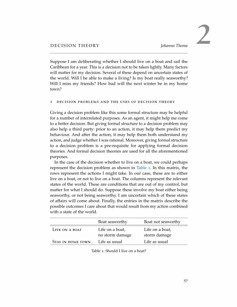
2D E C I S I O N T H E O RY Johanna Thoma
Suppose I am deliberating whether I should live on a boat and sail theCaribbean for a year. This is a decision not to be taken lightly. Many factorswill matter for my decision. Several of these depend on uncertain states ofthe world. Will I be able to make a living? Is my boat really seaworthy?Will I miss my friends? How bad will the next winter be in my hometown?
1 decision problems and the uses of decision theory
Giving a decision problem like this some formal structure may be helpfulfor a number of interrelated purposes. As an agent, it might help me cometo a better decision. But giving formal structure to a decision problem mayalso help a third party: prior to an action, it may help them predict mybehaviour. And after the action, it may help them both understand myaction, and judge whether I was rational. Moreover, giving formal structureto a decision problem is a pre-requisite for applying formal decisiontheories. And formal decision theories are used for all the aforementionedpurposes.
In the case of the decision whether to live on a boat, we could perhapsrepresent the decision problem as shown in Table 1. In this matrix, therows represent the actions I might take. In our case, these are to eitherlive on a boat, or not to live on a boat. The columns represent the relevantstates of the world. These are conditions that are out of my control, butmatter for what I should do. Suppose these involve my boat either beingseaworthy, or not being seaworthy. I am uncertain which of these statesof affairs will come about. Finally, the entries in the matrix describe thepossible outcomes I care about that would result from my action combinedwith a state of the world.
Boat seaworthy Boat not seaworthy
Live on a boat Life on a boat,no storm damage
Life on a boat,storm damage
Stay in home town Life as usual Life as usual
Table 1: Should I live on a boat?
57

58 johanna thoma
Since Savage’s (1954) decision theory, it has become standard to charac-terise decision problems with state-outcome matrices like the one I justintroduced. More generally, let A1 . . . An be a set of n actions that are opento the agent, and let S1 . . . Sm be m mutually exclusive and exhaustivestates of the world. These actions and states of the world combine toyield a set of n ·m outcomes O11 . . . Onm. Table 2 shows this more generalstate-outcome matrix.
S1 . . . Sm
A1 O11 . . . O1m...
.... . .
...
An On1 . . . Onm
Table 2: State-outcome matrix
Given such a representation of a decision problem, formal decisiontheories assume that agents have various attitudes to the elements of thestate-outcome matrix. Agents are assumed to have preferences over theoutcomes their actions might lead to. Depending on our interpretationof decision theory, we may also assume that agents can assign a utilityvalue to the outcomes, and a probability value to the states of the world.Decision theories then require the preferences the agent has over actions,which are assumed to guide her choice behaviour, to relate to those otherattitudes in a particular way.
1.1 Expected Utility Maximisation
Traditionally, the requirement that decision theories place on agents underconditions of uncertainty has been that agents should maximise theirexpected utility, or act as if they did. Decision theories which incorporatethis requirement are known under the heading of ‘expected utility theory’.In the special case where an agent is certain about the consequencesof each of her actions, this requirement reduces to the requirement tomaximise utility. Since we are always to some extent uncertain about theconsequences of our actions, I will focus on the uncertain case here.1
However, much of the following discussion will also apply to decision-
1 I understand decision-making under ‘uncertainty’ here to refer to any case where an agentis not certain what the consequences of her actions will be, or what state will come about. Adistinction is sometimes made between risk, uncertainty, ignorance and ambiguity, where‘risk’ refers to the case where objective probabilities are known, ‘uncertainty’ refers to thecase where an agent can make a subjective judgement about probabilities, an agent is ina state of ‘ignorance’ if she cannot make such probability assignments, and ‘ambiguity’occurs when an agent can make probability assignments for some states, but not others.

decision theory 59
making under certainty. Moreover, most of this entry will focus on expectedutility theory. Some alternative decision theories are discussed in Section 6.
As we will see, the requirement to maximise expected utility takesdifferent forms under different interpretations of expected utility theory.For now, let us assume that agents can assign utility values u(O) tooutcomes, and probability values p(S) to states of the world. The expectedutility is then calculated by weighting the utility of each possible outcomeof the action by the probability that it occurs, and summing them together.Expected utility theory instructs us to prefer acts with higher expectedutility to acts with lower expected utility, and to choose one of the actswith the highest expected utility.
In our example, suppose that I think that the chances that my boatis seaworthy are 50%, and that the relevant utilities are the ones givenin Table 3. In that case, the expected utility of living on a boat will be0.5 · 200 + 0.5 · 20 = 110, while the expected utility of staying in my hometown is 100. I conclude I should live on a boat.
Boat seaworthy Boat not seaworthy EU
Live on a boat 200 20 110
Stay in home town 100 100 100
Table 3: Decision problem with utilities
Formally, the expected utility EU(A) of an action can be expressed asfollows:
EU(Ai) =m
∑j=1
p(Sj) · u(Oij).
Expected utility theory requires agents to prefer acts for which thisweighted sum is higher to acts for which this weighted sum is lower,and to choose an action for which this weighted sum is maximised.
1.2 The Uses of Decision Theory
Now we can see how expected utility theory could be put to each of thedifferent uses mentioned above. The requirement to maximise expectedutility (or to act as if one did), however it is understood, is considered asa requirement of practical rationality by proponents of expected utilitytheory. In particular, the requirements of expected utility theory are ofteninterpreted to capture what it means to be instrumentally rational, thatis, what it means to take the appropriate means to one’s ends, whatever
While these differences will play a role later in this entry, it is not helpful to make thesedistinctions at this point.

60 johanna thoma
those ends may be. We will see how this may be cashed out in more detailin Section 3, when we discuss different interpretations of expected utilitytheory. For now, note that if we take the utility function to express theagent’s ends, then the requirement to maximise the expectation of utilitysounds like a natural requirement of instrumental rationality.
Sometimes, the requirements of expected utility theory are also under-stood as expressing what it means to have coherent ends in the first place.Constructivists about utility (see Section 3.1) often understand expectedutility theory as expressing requirements on the coherence of preferences.But on that understanding, too, expected utility theory does not make anyprescriptions on the specific content of an agent’s ends. It merely rules outcertain combinations of preferences. And so for those who think that someends are irrational in themselves, expected utility theory will at best be anincomplete theory of practical rationality.
If we understand the requirements of expected utility theory as require-ments of practical rationality, it seems like expected utility theory couldhelp me as an agent make better decisions. After I have formally repre-sented my decision problem, expected utility theory could be understoodas telling me to maximise my expected utility (or to act as if I did). In theabove example, we employed expected utility theory in this way. Expectedutility theory helped me decide that I should live on a boat. In this guise,expected utility theory is an action-guiding theory.
From a third party perspective, expected utility theory could also beused to judge whether an agent’s action was rational. Having representedthe agent’s decision problem formally, we judge an action to be rational ifit was an act with maximum expected utility. This understands expectedutility theory as a normative theory: a theory about what makes it the casethat somebody acted rationally.
It is important to note the difference between the action-guiding andthe normative uses of expected utility theory.2 An action can be rationalaccording to normative expected utility theory even if the agent did notuse expected utility theory as an action-guiding theory. One could evenhold that expected utility theory is a good normative theory while beinga bad action-guiding theory. This would be the case if most agents arebad at determining their expected utility, and do better by using simplerheuristics.3
2 Herbert Simon famously drew attention to this difference when he distinguished betweenprocedural and substantive rationality, drawing on a similar distinction made by Max Weber(1922/2005). See Simon (1976).
3 Starting with Tversky and Kahneman (1974), there has been a wealth of empirical literaturestudying what kind of heuristics decision-makers use when making decisions underuncertainty, and how well they perform. See, for instance, Payne, Bettman, and Johnson(1993) and Gigerenzer, Todd, and Group (2000).

decision theory 61
Expected utility theory is also often put to an explanatory or predictiveuse, especially within economics or psychology. If we assume that agentsfollow the requirements of expected utility theory, and we know enoughof their preferences or utility and probability assignments, we can usethe theory to predict their behaviour. In this context, philosophers havebeen interested more in whether decision theory can help us understand anagent’s actions. Interpreting an agent as maximising her expected utilityin a formal decision problem may reveal her motives in action, and thusexplain her action.
In fact, there is a tradition in the philosophy of action that claimsthat explaining another’s behaviour always involves rationalising herbehaviour to some extent. Davidson (1973) introduced the label ‘radicalinterpretation’ for the attempt to infer an agent’s attitudes, such as herbeliefs and desires, from her actions. He believed that this was onlypossible if we assume certain rationality constraints on how these attitudesrelate. Ramsey (1926/2010) had already used expected utility theory toinfer an agent’s probabilities, and thus, he argued, her beliefs from herbehaviour. Lewis (1974) showed that expected utility theory capturesDavidson’s constraints on the relationship between beliefs and desires,and thus can be used to elicit beliefs and desires. Davidson himself laterargued, in Davidson (1985), that expected utility theory can be extendedto further elicit an agent’s meanings, that is, her interpretation of sentences.This is sometimes known as the interpretive use of decision theory.
And so in the philosophical literature, expected utility theory has beenused as an action-guiding theory, a normative theory, and an interpretivetheory.4 Other decision theories have been put to the same uses. As wewill see in Section 6, there are alternatives to expected utility theory thatoffer rival prescriptions of practical rationality. However, most alternativesto expected utility theory have been introduced as primarily descriptivetheories, that are used to predict and explain behaviour that need not berational.
Now that we have seen what kinds of uses expected utility theory canbe put to, the next section will look at some influential applications ofexpected utility theory.
1.3 Some Applications
Expected utility theory has proven to be an enormously fruitful theory,that has been applied in various different fields and disciplines. Originally,it found application mostly in the theory of consumer choice. This field
4 Bermudez (2009) draws a similar tri-partite distinction between the normative, action-guiding and explanatory/predictive dimensions of decision theory. Similarly, Buchak(2016) distinguishes between the normative and interpretive uses of decision theory.

62 johanna thoma
of economics studies why consumers choose some goods rather thanothers, and helps to predict market outcomes. Expected utility theory hasbeen used to explain the shape of demand curves for goods. The demandfor insurance, in particular, is difficult to understand without a formaltheory of choice under uncertainty. Expected utility theory has also helpedto explain some phenomena that had previously seemed surprising. Aclassic example here is adverse selection, which occurs when there is aninformation asymmetry between buyers and sellers in the market. In thesekinds of situations, sellers of high quality goods may be driven out ofthe market. Akerlof (1970) first explained this phenomenon, and a richliterature has developed since. Einav and Finkelstein (2011) provide ahelpful overview of work on adverse selection in insurance markets.
Decision theory has also found application in many fields outside ofeconomics. For instance, in politics, it has been used to study voting andvoter turn-out,5 in law it has been used to study judicial decisions,6 and insociology it has been used to explain class and gender differences in levelsof education.7
Expected utility theory has also been influential in philosophy. Apartfrom it being an important contender as a theory of practical rationality,expected utility theory plays an important role in ethics, in particular inconsequentialist ethics. Along with Jackson (1991), many consequentialistsbelieve that agents ought to maximise expected moral goodness. Moreover,expected utility theory has been applied to the question of what agentsought to do in the face of moral uncertainty—uncertainty about what oneought to do, or even about which moral theory is the right one.8
Recently, expected utility theory has found application in epistemologyin the form of epistemic decision theory. Here, agents are modeled as receiv-ing epistemic utility from being in various epistemic states, such as beingcertain of the proposition that my boat is sea-worthy. I will receive a highepistemic utility from being in that state in the case where my boat in factturns out to be seaworthy, and low epistemic utility when my boat turnsout not to be seaworthy. Agents are then modeled as maximising theirexpected epistemic utility. Epistemic utility theory has been used to justifyvarious epistemic norms, such as probabilism (the norm that an agent’scredences should obey the probability calculus), and conditionalisation(the norm that agents should update their credences by conditionalizingtheir old credence on the new evidence they received). For an overview ofthese arguments, see Pettigrew (2011).
5 Downs (1957) counts as the first systematic application of decision theoretic models fromeconomics to politics. For recent work on voting specifically, see Feddersen (2004).
6 See, for instance, Epstein, Landes, and Posner (2013).7 See, for instance, Breen and Goldthorpe (1997).8 See, for instance, Lockhart (2000), and Sepielli (2013) for a criticism of Lockhart’s approach.

decision theory 63
1.4 Formulating Decision Problems
How should the decision problems that formal decision theories dealwith be formulated in the first place? In order to apply a formal decisiontheory, the choices an agent faces need to already be represented as aformal decision problem. Table 1 offered one representation of my choiceof whether to live on a boat. But how can we be sure it was the right one?
For his decision theory, Savage (1954) assumed that states are descrip-tions of the world that include everything that might be relevant to theagent. Similarly, he thought that descriptions of outcomes are descriptionsof “everything that might happen to the person” (p. 13). Joyce (1999, p. 52)cashes out a rule for specifying outcomes that also appeals to relevance.He claims that a description of an outcome should include everything thatmight be relevant to the agent, in the following sense: whenever there issome circumstance such that an agent would strictly prefer an outcomein the presence of that circumstance to the same outcome in the absenceof that circumstance, the outcome has been underspecified. Importantly,this implies that an agent’s evaluation of an outcome should be indepen-dent of the state it occurs in, and the act that brought it about. All ofthis means that the sets of states and outcomes will end up being veryfine-grained. Moreover, Savage also thinks of actions as functions fromstates to outcomes. This means that in each state, each action leads to aunique outcome. To ensure this, the set of actions, too, will have to be veryfine-grained.
Note that this means that the decision problem I presented in Table 1
was hopelessly underspecified. When it comes to the decision of whetherto live on a boat for a year or not, I do not only care about whether my boatwill have storm damage or not. I also care, for instance, about whether Iwill have enough money for the year. I will evaluate the outcome “Life ona boat, no storm damage” differently depending on whether I will haveenough money for the year or not. In fact, the exact amount of money Iwill have is going to matter for my decision. And so my decision problemshould really distinguish between many different states of affairs involvingme having more or less money, and the many different outcomes thatoccur in these states of affairs.
Jeffrey (1965/1983), who offered a famous alternative to Savage’s deci-sion theory (see Section 2.4), and treated states, acts, and outcomes all aspropositions, went so far as to define outcomes such that they entail anact and a state. An act and a state are also supposed to entail the outcome,and so we can simply replace outcomes with the conjunction of an act anda state in the decision matrix.
These ways of individuating outcomes will obviously lead to very largedecision matrices for any real life decision. There are two reasons why we

64 johanna thoma
might find this problematic. The first reason has to do with the efficiencyof the decision-making process. If we want our decision theory to bean action-guiding theory, then decision problems can’t be so complexthat ordinary agents cannot solve them. An action-guiding theory shouldbe efficient in its application. Efficiency may also be a concern for theinterpretive project. After all, this project wants to enable us to interpreteach other’s actions. And so doing so should not be overly complicated.
Savage called decision problems that specify every eventuality thatmight be relevant to an agent’s choice “grand world” decision problems.Joyce (1999) holds that we should really be trying to solve such a grand-world problem, but acknowledges that real agents will always fall shortof this. Instead, he claims, they solve “small world” decision problems,which are coarsenings of grand-world decision problems. If we treat acts,states and outcomes as propositions, this means that the acts, states andoutcomes of the small world decision problems are disjunctions of the acts,states, and outcomes of the grand-world decision problem. The decisionproblem described in Table 1 is such a small-world decision problem.
Joyce (1999, p. 74) holds that an agent is rational in using such small-world decision problems to the extent that she is justified in believingthat her solution to the small-world decision problem will be the same asher solution to the grand-world decision problem would be. This permitsthe use of small world decision problems both for the action-guiding andnormative purposes of decision theory whenever the agent is justified inbelieving that they are good enough models of the grand-world decisionproblem.
Joyce argues that this condition is met in Jeffrey’s decision theory ifan agent correctly evaluates all coarse outcomes and actions, while it isnot generally met in Savage’s decision theory. As will be explained inSection 2.4, this is due to the feature of partition invariance, which Jeffrey’stheory has and Savage’s theory does not. Despite these arguments, ifefficiency in decision-making is an important concern, as it is for an action-guiding theory, one might think that an agent should sometimes base herdecision on a small-world decision problem even if she is fairly certain thather decision based on the grand-world decision problem will be different.She might think that her solution to a small-world decision problem willbe close enough to that of the grand-world decision problem, while solvingthe small-world decision problem will save her costs of deliberation.
The second argument against having too fine-grained a decision prob-lem is that this makes expected utility theory not restrictive enough. Aswill be explained in more detail in Section 2, the axioms used in the repre-sentation theorems of expected utility theory concern what combinationof preferences are permissible. If preferences attach to outcomes, andoutcomes can be individuated as finely as we like, then the danger is that

decision theory 65
the norm to abide by the axioms of decision theory does not constrain ouractions much.
For instance, consider the following preference cycle, where a, b and care outcomes, and ≺ expresses strict preference:
a ≺ b ≺ c ≺ a.
Preference cycles such as this are ruled out by the transitivity axiom, whichall representation theorems we shall look at in Section 2 share. Whenoutcomes can be individuated very finely, the following two problemsmay arise. Firstly, a number of authors have worried that any potentialcircularity in an agent’s preferences can be removed by individuatingoutcomes more finely, such that there is no circularity anymore. Secondly,and relatedly, fine individuation may mean that no outcome can ever berepeated. In that case, an agent cannot reveal a preference cycle in heractions, and so we cannot interpret her as being irrational.
To see this, note that if we treat the first and the second occurrence ofoutcome a above as two different outcomes, say a1 and a2, the circularityis removed:
a1 ≺ b ≺ c ≺ a2.
The worry is that this can always be done, for instance by distinguishing“option a if it is compared to b” from “option a if it is compared to c”. Ifthis strategy is always available, in what sense is the transitivity axiom atrue restriction of the agent’s preferences and actions? If we can’t showthat decision theory puts real restrictions on an agent’s choices, then thisis a problem especially for the action-guiding and normative projects.
A number of authors9 have held that this problem shows that the axiomsof decision theory on their own cannot serve as a theory of practicalrationality (even a partial one), but have to be supplemented with a furtherprinciple in order to serve their function. Broome (1991, chapter 5) notesthat the problem can be dealt with by introducing rational requirements ofindifference. Rational requirements of indifference hold between outcomesthat are modeled as different, but that it would be irrational for the agentto have a strict preference between. If there was a rational requirement ofindifference between a1 and a2, for instance, the preference cycle would bepreserved.
However, we may also restrict how finely outcomes can be individuatedto solve the problem, by not allowing a distinction between a1 and a2.Broome (1991, chapter 5) advocates a rule of individuation by justifiersthat serves the same role as the rational requirements of indifference.According to this rule, two outcomes can only be modeled as distinct if itis not irrational to have a strict preference between them.
9 See, especially, Broome (1991), Pettit (1991) and Dreier (1996).

66 johanna thoma
Pettit (1991) proposes an alternative rule for individuation: two outcomesshould be modeled as distinct just in case they differ in some quality theagent cares about, where caring about a quality cannot itself be cashedout in terms of preferences over outcomes. And Dreier (1996) argues thattwo outcomes should be distinguished just in case there are circumstanceswhere an agent has an actual strict preference between them. Note thatthis rule for individuation is equivalent to the one proposed by Joyce, butPettit’s and Broome’s rules may lead to coarser grained individuationsof decision problems. The coarser grained the individuations, the morerestrictive the axioms of expected utility theory end up being.
2 representation theorems
2.1 The Preference Relation
In decision theory, representation theorems are proofs that an agent’spreferences are representable by a function that is maximised by the agent.In the case of expected utility theory, they are proofs that an agent’spreferences are such that we can represent her as maximising an expectedutility function. As we will see in Section 3, many decision theorists believethat utility is nothing more than a convenient way to represent preferences.Representation theorems are crucial for this interpretation of utility. Thesignificance of the representation theorems will be further discussed inSection 3.2.
A weak preference relation is a binary relation <, which is usuallyinterpreted either as an agent’s disposition to choose, or her judgementsof greater choiceworthiness.10 An agent weakly prefers x to y if she findsx at least as choiceworthy as y, or if she is disposed to choose x when xand y are available.
We can also define an indifference relation ∼ and a strict preferencerelation in terms of the weak preference relation <:
1. x ∼ y if and only if x < y and y < x,
2. x y if and only if x < y and not y < x.
Representation theorems take such preference relations as their startingpoint. They then proceed by formulating various axioms that pose re-strictions on the preference relation, some of which are interpreted as
10 Many economists interpret preference as ‘revealed preference’, and claim that an agentcounts as preferring x to y just in case she actually chose x when y was also available. Suchpure behaviourism is usually rejected in the philosophical literature because it takes awayfrom the explanatory power of preferences, and does not allow for counter-preferentialchoice. For a critique of the notion of revealed preference, see Hausman (2000).

decision theory 67
conditions of rationality. Let X be the domain of the preference relation.What representation theorems prove is the following. If an agent’s prefer-ences conform to the axioms, there will be a probability function and autility function such that:
for all x and y ∈ X, EU(x) ≥ EU(y) if and only if x < y.
All the representation theorems described in the following assume thatthe preference relation is a weak ordering of the elements in its domain.That means that the preference relation is transitive and complete.
Transitivity. For all x, y and z ∈ X, x < y and y < z implies that x < z.
Completeness. For all x and y ∈ X, x < y or y < x.
Section 4 will discuss potential problems with both completeness andtransitivity.
Different representation theorems differ both in terms of the domainover which the preference relation is defined, and in terms of the otheraxioms needed for the representation theorem. They also differ in howmany of the agent’s attitudes other than preferences they take for granted.Consequently, they result in representation theorems of different strength.
2.2 Von Neumann and Morgenstern
One of the first representation theorems for expected utility is due to vonNeumann and Morgenstern (1944) and takes probabilities for granted.11
In this representation theorem, the objects of preference are lotteries, whichare either probability distributions L = (p1, . . . , pm) over the m outcomes,or probability distributions over these ‘simple’ lotteries. Probabilities arethus already part of the agent’s object of preference.
While it helps to think of lotteries in the ordinary sense of monetarygambles where there is a known probability of winning some prize, vonNeumann and Morgenstern intended for their representation theorem tohave wider application. In our original example, if there is a 50% chancethat my boat is seaworthy, then I face a 50/50 lottery over the outcomesdescribed in Table 1. Note furthermore that, since we are dealing directlywith probability distributions over outcomes, there is no need to speak ofstates of the world.
While von Neumann and Morgenstern’s representation theorem is per-haps most naturally understood given an objective interpretation of proba-bility, their representation theorem is in fact compatible with any interpre-tation of probability. All we need is to already have access to the relevant
11 An earlier representation theorem is due to Ramsey (1926/2010) and derives probabil-ities as well as utilities. It is often considered as a precursor to Savage’s and Bolker’srepresentation theorems, discussed below. See R. Bradley (2004).

68 johanna thoma
(precise) probabilities when applying the representation theorems. If wethink of probability as the agent’s subjective degrees of belief, we alreadyneed to know what those subjective degrees of belief are. If we think of itas objective chance, we need to already know what those objective chancesare.
What von Neumann and Morgenstern go on to prove in their represen-tation theorem is that, provided an agent’s preferences over lotteries abideby certain axioms, there is a utility function over outcomes such that anagent prefers one lottery over another just in case its expected utility ishigher. One crucial axiom needed for this representation theorem is theindependence axiom, discussed in Section 5.1.
Note that the result is not that there is one unique utility function whichrepresents the agent’s preferences. In fact, there is a family of utility func-tions which describe the agent’s preferences. According to von Neumannand Morgenstern’s representation theorem, any utility function whichforms part of an expected utility representation of an agent’s preferenceswill only be unique up to positive, linear transformations. The differentutility functions that represent an agent’s preferences will thus not allshare the same zero point. What outcome will yield twice as much utilitywill then also differ between different utility functions. It is therefore oftenclaimed that these properties of utility functions represent nothing “real”.What is invariant between all the different utility functions that representthe agent’s preferences, however, are the ratios of utility differences, whichcan capture the curvature of the utility function. Such ratios are often usedto measure an agent’s level of risk aversion.12
2.3 Savage
While von Neumann and Morgenstern’s representation theorem providesa representation of an agent’s preferences where probabilities are alreadygiven, Savage (1954) infers both a utility function and probabilities froman agent’s preferences.13 As we have already seen, the standard tripartitedistinction of actions, outcomes and states of the world goes back toSavage. Instead of assuming, like von Neumann and Morgenstern did,that we can assign probabilities to outcomes directly, we introduce a set
12 Risk aversion is further discussed in Section 5.3. Also see Mas-Colell, Whinston, and Green(1995), chapter 6 for more detail on expected utility theory’s treatment of risk aversion.
13 This is why von Neumann and Morgenstern’s theory is sometimes referred to as a theoryof decision-making under risk, and Savage’s is referred to as a theory of decision-makingunder uncertainty. In the former, probabilities are already known, in the latter, subjectiveprobabilities can be assigned by the agent. However, note that, as we pointed out above,von Neumann and Morgenstern’s theory can also be applied when probabilities aresubjective.

decision theory 69
of states of the world, which determine what outcome an act will lead to.The agent does not know which of the states of the world will come about.
Savage takes the agent’s preferences over acts as input, and introducesa number of axioms on these preferences. He derives both a probabilityfunction over states, which abides by the standard axioms of probability,and a utility function over outcomes which, like the one von Neumannand Morgenstern derived, is unique up to positive linear transformations.Together, they describe an expected utility function such that an act ispreferred to another just in case it has a higher expected utility. Importantly,the agents in Savage’s decision theory abide by the sure-thing principle,which serves a role similar to the independence axiom in von Neumannand Morgenstern’s representation theorem, and will also be discussed inSection 5.1.
Acts, states and outcomes are all treated as theoretical primitives inSavage’s framework. But Savage’s representation theorem relies on anumber of controversial assumptions about the act, state and outcomespaces and their relation. For one, probabilities apply only to states ofthe world, and utilities apply only to outcomes. Preferences range overboth acts and outcomes. Savage assumed that an act and a state togetherdetermine an outcome. Most controversially, Savage assumes that thereare what he calls constant acts for each possible outcome, that is, actswhich bring about that outcome in any state of the world. For instance,there must be an act which causes me great happiness even in the eventthat the apocalypse happens tomorrow. What makes things worse, bycompleteness, agents are required to have preferences over all these acts.Luce and Suppes (1965) take issue with Savage’s theory for this reason.
While the results of Savage’s representation theorem are strong, theyrely on these strong assumptions about the structure of the act space. Thisis one reason why many decision theorists prefer Jeffrey’s decision theoryand Joyce’s modification thereof.
2.4 Jeffrey, Bolker, and Joyce
Jeffrey’s decision theory, developed in Jeffrey (1965/1983), uses an axioma-tisation by Bolker (1966). While he does not rely on an act space as richas Savage’s, Jeffrey preserves the tripartite distinction of acts, states andoutcomes. However, for him, all of these are propositions, which meanshe can employ the tools of propositional logic. Moreover, preferences,utility and probability all range over all three. Agents end up assigning

70 johanna thoma
probabilities to their own acts,14 and assigning utilities to states of theworld.
Jeffrey’s theory is sometimes known as conditional expected utilitytheory, because agents who follow the axioms of his decision theory arerepresented as maximisers of a conditional expected utility. In Savage’sdecision theory, the utilities of outcomes are weighted by the unconditionalprobability of the states in which they occur. This is also the formulationwe presented in Section 1.1. In the example there, we weighted the possibleoutcomes by the probability of the state they occur in. For instance, weweighted the outcome of enjoying a year on a boat without damages bythe probability of my boat being seaworthy.
Jeffrey noted that the unconditional nature of Savage’s decision theorymay produce the wrong results in cases where states are made more orless likely by performing an action. In our example, suppose that, forwhatever reason, my choosing to live on a boat for a year makes it morelikely that my boat is seaworthy. The unconditional probability of the boatbeing seaworthy is lower than the probability of it being seaworthy givenI decide to live on the boat. And thus using the unconditional probabilitymay lead to the judgement that I shouldn’t spend the year on the boat,because the probability of it not being seaworthy is too high—even if theboat will be very likely to be seaworthy if I choose to do so. To avoid thisproblem, Jeffrey argued, it is better to use probabilities that are in somesense conditional on the action whose expected utility we are evaluating.We should weight the outcome of spending a year on a boat withoutdamage by the probability of the boat being seaworthy given that I chooseto live on the boat for a year.15
Let the probability of a state given an act be pA(S). There is muchdisagreement on how this probability is to be interpreted. The maindisagreement is whether it should be given a causal or an evidentialinterpretation. I postpone this discussion to Section 3.3. But let me notehere that Jeffrey himself falls on the evidential side. Conditional expectedutility theory advises us to maximise the following:
EU(Ai) =m
∑j=1
pAi(Sj) · u(Oij).
Jeffrey interprets this conditional expected utility as an act’s ‘news value’,that is, as measuring how much an agent would appreciate the news thatthe act is performed.
14 This is a controversial feature of the theory. See Spohn (1977) for criticism of this assump-tion.
15 Savage’s own solution to the problem is that, for his formalism to apply, states and actsneed to be specified such that there is no dependence between an action being performedand the likelihood of a state. Jeffrey’s response is more elegant in that it requires no suchrestriction on what kinds of decision problems it can be applied to.

decision theory 71
The conditional nature of Jeffrey’s decision theory is also what leads toits partition invariance.16 In Jeffrey’s theory, the value of a disjunction isalways a function of the value of its disjuncts. For instance, the value ofa coarse outcome O1−10 which is a disjunction of outcomes O1, . . . , O10 isa function of the values of the outcomes O1, . . . , O10. But we could alsosubdivide the coarse outcome O1−10 differently. O1−10 is also a disjunctionof the coarse outcomes O1−5 and O6−10, which are themselves disjunctionsof O1, . . . , O5 and O6, . . . , O10 respectively. And so we can also calculatethe value of O1−10 from the values of O1−5 and O6−10. Partition invariancemeans that we get the same value in either case. The value of O1−10
can be represented as a function of the values of any of its subdivisions.This means that, as long as utilities are assigned correctly to disjunctions,Jeffrey’s decision theory gives equivalent recommendations no matterhow finely we individuate outcomes, states and actions. Joyce argues thatfor this reason, the use of small-world decision problems is legitimatein Jeffrey’s decision theory (see Section 1.4), and that that is a majoradvantage over Savage’s unconditional, and partition variant decisiontheory.
Jeffrey’s and Bolker’s representation theorem is less strong than Savage’s.It does not pin down a unique probability function. Nor does it resultin a utility function that is unique up to positive linear transformations.Instead, it only ensures that probability and utility pairs are unique up tofractional linear transformations.17
Joyce (1999) argues that this shows that we need to augment Jeffrey’s andBolker’s representation theorem with assumptions about belief, and notmerely preference. Unlike von Neumann and Morgenstern, however, hedoes not propose to simply assume probabilities. Instead, he introduces a‘more likely than’ relation, on which we can formulate a number of axioms,just as we did for the preference relation. The resulting representationtheorem results in a unique probability function and a utility functionwhich is unique up to positive linear transformations.18
We have introduced the most prominent representation theorems forexpected utility theory.19 What do these representation theorems show?Each of them shows that if an agent’s preferences abide by certain axioms,and certain structural conditions are met, her preferences can be repre-sented by a utility (and probability) function (or families thereof) suchthat she prefers an act to another just in case its expected utility is higher.
16 See Joyce (1999), pp. 121-122.17 A fractional linear transformation transforms u to a·u+b
c·u+d , with a · d− b · c > 0.18 Also see R. Bradley (1998), for an alternative way to secure uniqueness.19 A helpful, more technical and more detailed overview of representation theorems can be
found in Fishburn (1981).

72 johanna thoma
Agents who abide by the axioms can thus be represented as expectedutility maximisers.
What these kinds of results show depends to some extent on the purposewe want to put our theory to. But it also depends on how we interpretthe utilities and probabilities expected utility theory deals with. Section 3
gives an overview of these interpretations and then returns to the questionof what the representation theorems can show.
3 interpretations of expected utility theory
3.1 Interpretations of Utility
Some of the earliest discussions of choice under uncertainty took placein the context of gambling. The idea that gamblers maximise some ex-pected value first came up in correspondence between Fermat and Pascal(1654/1929). Pascal, who formulated the expected value function in thiscontext, thought of the value whose expectation should be maximised asmoney. This is natural enough in the context of gambling. Similarly, in thiscontext it is natural to think of the probabilities involved as objective, andfixed by the parameters of the game.
However, money was soon replaced by the notion of utility as the valuewhose expectation is to be maximised. This happened for two interrelatedreasons. First, the same amount of money may be worth more or less tous depending on our circumstances. In particular, we seem to get lesssatisfaction from some fixed amount of money the more money we alreadyhave. Secondly, the norm to maximise expected monetary value has somecounterintuitive consequences. In particular, we can imagine gambles thathave infinite monetary value, that we would nevertheless only pay a finiteprice for. Nicolas Bernoulli first demonstrated this with his famous St.Petersburg Paradox.20
In response to these problems, Daniel Bernouilli (1738/1954) and GabrielCramer independently proposed a norm to maximise expected utilityrather than expected monetary value. However, this raises the problem ofhow to interpret the notion of utility. One strand of interpretations takesutility to be a real psychological quantity that we could measure. Let uscall such interpretations of utility ‘realist’. Early utilitarians adopted arealist interpretation of utility. For instance, Bentham (1789/2007) and Mill(1861/1998) thought of it as pleasure and the absence of pain.
20 Bernoulli proposed a gamble in which a coin is thrown repeatedly. If it lands heads thefirst time, the player gets $2. If it lands tails, the prize is doubled, and the coin thrownagain. This procedure is repeated indefinitely. The expected value of the resulting gambleis thus $2 · 1
2 + $4 · 14 + $8 · 1
8 + . . ., which is infinite. However, most people would onlypay a (low) finite amount for it.

decision theory 73
Note, however, that these utilitarians were interested in defining utilityfor the purpose of an ethical theory rather than a theory of rationality. Oneproblem with interpreting utility as pleasure in the context of expectedutility theory is that the theory then seems to imply that true altruism cannever be rational. If rationality requires me to maximise my own expectedpleasure, then I can never rationally act so as to increase somebody else’shappiness at my own expense.
For this and other reasons modern realists typically think of utility as ameasure of the strength of an agent’s desire or preference, or her level ofsatisfaction of these desires or preferences. I may strongly desire somebodyelse’s happiness, or be satisfied if they achieve it, even if that does notdirectly make me happy.21 Jeffrey (1965/1983), for instance, speaks ofdesirabilities instead of utilities, and interprets them as degrees of desire(p. 63). The corresponding realist interpretation of the probabilities inexpected utility theories is usually that of subjective degrees of belief.
The representation theorems described in Section 2 have, however, madea different kind of interpretation of utility (and probability) possible, andpopular. These representation theorems show that preferences, if theyconform to certain axioms, can be represented with a probability andutility function, or families thereof. And so, encouraged by these results,many decision theorists think of utility and probability functions as meretheoretical constructs that provide a convenient way to represent binarypreferences. For instance, Savage (1954) presents his theory in this way.Importantly, on this interpretation, we cannot even speak of probabilitiesand utilities in the case where an agent’s preferences do not conform withthe axioms of expected utility theory. Let us call these interpretations ofutility and probability ‘constructivist’.22
3.2 The Significance of the Representation Theorems
Whether we adopt a realist or a constructivist interpretation of utilitymatters for how expected utility theory can serve the three purposes ofdecision theory described in Section 1.2, and for what the representationtheorems presented in Section 2 really establish. Let us first look at theinterpretive project. As already mentioned, those interested in the interpre-tive project have mostly been interested in inferring an agent’s beliefs and
21 This is also the interpretation adopted by several later utilitarians, such as Hare (1981) andSinger (1993).
22 See Dreier (1996) and Velleman (1993/2000) for defenses of constructivism. Buchak (2013)draws slightly different distinctions. For her, any view on which utility is at least partiallydefined with respect to preferences counts as constructivist. Since this is compatible withholding that utility is a psychologically real quantity, she allows for constructivist realistpositions. The position that utility expresses strength of desire, for her, is such a position. Iwill count this position as realist, and not constructivist.

74 johanna thoma
desires from her choice behaviour. If that is the goal, then the probabilitiesand utilities involved in decision theory should at least be closely relatedto desires and beliefs. Under the assumption that agents maximise theirutility and probability functions, thus understood, we can hypothesise,perhaps even derive, probability and utility functions that motivate anagent’s actions.
How could the representation theorems we described in Section 2 helpwith this project? They go some way towards showing that beliefs anddesires can be inferred from an agent’s choice behaviour. But the followingassumptions are also needed for this project to succeed:
1. The agent’s choice behaviour must reflect her preferences, at leastmost of the time. This assumption is more likely to be met if we thinkof preferences as a dispositions to choose, rather than as judgementsof choiceworthiness.
2. The axioms of the representation theorems must be followed by theagent, at least most of the time. If we want to use expected utilitytheory to deduce an agent’s beliefs and desires, then the agent’spreferences have to be representable by an expected utility function.While we can interpret the axioms as rationality constraints, thesecannot be the kinds of constraints that people fail to meet most ofthe time. In particular, if we want to employ expected utility theoryfor Davidson’s ‘radical interpretation’, then the choice behaviour ofagents who fail to abide by the axioms will turn out to be unintelli-gible.
3. The probabilities and utilities furnished by the representation theo-rem must correspond to the agent’s actual beliefs and desires.
Assumption 2 is controversial for the reasons described in Section 4
and Section 5. But assumption 3 is also problematic. The representationtheorems only show that an agent who abides by the axioms of thevarious representation theorems can be represented as an expected utilitymaximiser. But this is compatible with the claim that the agent can berepresented in some other way. It is not clear why the expected utilityrepresentation should be the one which furnishes the agent’s beliefs anddesires.23
To answer this challenge, the best strategy seems to be to providefurther arguments in favour of expected utility maximisation, and in
23 This question was raised, for instance, by Zynda (2000), Hajek (2008) and Meacham andWeisberg (2011). Zynda (2000) argues that the representation theorems alone cannot showthat agents do or should have probabilistic degrees of belief. Meacham and Weisberg (2011)provide a number of arguments why the representation theorems alone cannot serve asthe basis of decision theory.

decision theory 75
favour of probabilistic beliefs, apart from the plausibility of the axiomsof the representation theorems. Suppose we think it is plausible thatagents should have probabilistic degrees of belief, and should maximisethe expected degree of satisfaction of their desires. And suppose we alsothink that our preferences are closely related to our desires. Then if, givensome plausible axioms, these preferences can be given an expected utilityrepresentation, we seem to have good reason to think that the utilities andprobabilities furnished by the representation theorem correspond to ourdegrees of belief and strength of desire.
Setting aside the question of why we might want to have probabilisticdegrees of belief, what could such realist arguments for expected utilitymaximisation be? Note that, for the purposes of the interpretive project,these arguments have to not only be normatively compelling, but alsoconvince us that ordinary agents would be expected utility maximisers.One type of argument appeals to the advantages of being an expectedutility maximiser when making decisions in a dynamic context. Thesewill be covered in Section 7. Pettigrew (2014) makes another argument:for most realists, utility is supposed to capture everything an agent caresabout. If that is true, then it seems plausible to say that in uncertainsituations, I should be guided by my best estimate of how much utilityI will get. We can appeal to results in de Finetti (1974) to argue that anagent’s best estimate of a quantity is her subjective expectation. This is sobecause any estimate of the quantity that is a weighted sum different fromthe expectation will be accuracy dominated by an expectational estimate:the expectational estimate will be closer to the true value no matter whathappens. Thus, I should maximise my expected utility.
So far, we have assumed a realist interpretation of utility and probability.Note, however, that expected utility theory could still be explanatorilyuseful even if a constructivist interpretation of utility and probability areadopted. It is often argued that the representation theorems show thatthe utility and probability functions allow for a simpler and more unifiedrepresentation of an agent’s preferences: all the agent’s preferences canbe described with one utility and probability function. This could be seento make them more intelligible. In fact, Velleman (1993/2000) argues thatbeing an expected utility maximiser makes an agent more intelligible toherself and others, and that this gives her a reason to be an expected utilitymaximiser.
Let us now turn to the action-guiding and normative projects. Theseprojects will lead to quite different prescriptions depending on whetherutility is interpreted in a realist or in a constructivist sense. Suppose thatwe are constructivists about utility. In that case, there is a sense in whichthe prescription to maximise expected utility does not make any sense.If one abides by the axioms of one’s favourite representation theorem,

76 johanna thoma
one’s preferences are representable as expected utility maximising. Tomaximise expected utility, there is nothing more one needs to do, apartfrom act according to the preferences over acts one already has. But if one’spreferences do not abide by the axioms, on the other hand, one simplydoes not have a utility function whose expectation one could maximise.
Consequently, constructivists often interpret the prescription of expectedutility theory as a prescription to have preferences such that one can berepresented as an expected utility maximiser. That is, one should abide bythe axioms of expected utility theory. For the action-guiding project, thismeans that, as an agent, I should have preferences such that they abide bythe axioms of expected utility theory. For the normative project, it meansthat we judge an agent to be irrational if she has preferences that violatethe axioms. This is why constructivists often interpret expected utilitytheory as a theory about what it means to have coherent preferences orends, rather than as a theory of means-ends rationality.
For realists, however, the prescription to maximise expected utilitymakes sense even independently of the representation theorems canvassedin Section 2. Consider first the action-guiding project, which aims tointerpret expected utility theory as a theory that can guide an agent indeciding what to do. If utility is just my strength of desire, and probabilityis my degree of belief, and I have introspective access to these, then I candetermine the expected utility of the various acts open to me. I can do sowithout considering the structure of my preferences, and whether theyabide by the axioms of expected utility theory. Expected utility theory isthen action-guiding without appeal to representation theorems. But notethat the advice to maximise expected utility is only useful to agents ifthey really have such intuitive access to their own degrees of belief andstrength of desire.24
Similarly, if we are realists and our interests are normative, we can judgean agent to be irrational by considering her utilities and degrees of belief,and determining whether she failed to maximise expected utility. Thisis because there will be facts about the agent’s utilities and probabilitieseven if she fails to maximise expected utility. Realists about utility andprobability can also help themselves to the realist arguments for expectedutility maximisation just mentioned. For them, the normative force ofexpected utility theory does not depend solely on the plausibility of theaxioms of expected utility theory. If we adopt a realist interpretation ofutility and probability, it is also easier to argue that expected utility theoryprovides us with a theory of instrumental rationality. Maximising expectedutility could be seen as taking the means towards the end of achievingmaximum utility. However, realists will also have to provide an argumentthat this is a goal rational agents ought to have.
24 Also see Bermudez (2009) on this claim.

decision theory 77
3.3 Causal and Evidential Interpretations of Expected Utility Theory
We have said that the probabilities involved in expected utility theory areusually interpreted as subjective degrees of belief, at least by realists. As wehave seen, Jeffrey, Joyce, and others have advocated a conditional expectedutility theory. In conditional expected utility theory, agents determinean act’s expected utility by weighting utilities by the different states’probabilities conditional on the act in question being performed. Above,we called this probability pA(S). How this probability is to be interpretedis a further important interpretive question. The main disagreement isabout whether it should be given a causal or an evidential interpretation.Jeffrey himself had worked with an evidential interpretation, while causaldecision theorists, such as Gibbard and Harper (1978/1981), Armendt(1986), or Joyce (1999)25 have given it a causal interpretation.
The difference between these two interpretations is brought out by thefamous Newcomb Problem, first introduced by Nozick (1969). In thisproblem, we imagine a being who is very reliable at predicting yourdecisions, and who has already predicted your choice in the followingchoice scenario. You are being offered two boxes. One is opaque and eitherhas no money in it, or $1,000,000. The other box is clear, and you can seethat it contains $1,000. You can choose to either take only the opaque box,or to take both boxes. Under normal circumstances, it would seem clearthat you should take both boxes. Taking the clear box gives you $1,000
more no matter what.The complication, however, is that the being’s prediction about your
action determines whether there is money in the opaque box or not. If thebeing predicted that you will take two boxes, then there is no money inthe opaque box. If the prediction was that you will take only the opaquebox, there will be money in it. Since the being’s prediction is reliable, thosewho take only one box tend to end up with more money than those whotake two boxes.
Note that while this case is unrealistic, there are arguably real-life casesthat resemble the Newcomb Problem in its crucial features. In these cases,the acts available to an agent are correlated with good or bad outcomeseven though these are not causally promoted by the act. This happens inmedical cases, for instance, if a behavioural symptom is correlated with adisease due to a common cause. Before the causal link between smokingand lung cancer was firmly established, interested parties hypothesisedthat there may be a common cause which causes both lung cancer, and thedisposition to smoke. If that were right, smoking would not cause lung
25 Joyce also first showed that the two interpretations can be given a unified treatment in amore general conditional expected utility theory.

78 johanna thoma
cancer, but merely give you evidence that you are more likely to developit.26
Evidential and causal decision theory come apart in their treatment ofthese cases. Evidential decision theory traditionally interprets pA(S) as astandard conditional probability:
pA(S) =p(A&S)
p(A).
According to this interpretation, the probability of the state where there is$1,000,000 in the opaque box conditional on taking only one box is muchhigher than the probability of the state where there is $1,000,000 in theopaque box conditional on taking two boxes. This is because the act oftaking only one box provides us with evidence that the prediction wasthat you would take only one box, in which case there is money in theopaque box. And so expected utility maximisation would tell you to takeonly one box.
Causal decision theorists take issue with this, because at the time ofdecision, the agent’s actions have no more influence on whether thereis money in the opaque box or not. Either there is or there isn’t alreadymoney in the box. In either case, it is better for you to take two boxes, asTable 4 illustrates. This kind of dominance reasoning speaks in favour oftaking both boxes.
Prediction: one box Prediction: two boxes
Take one box $1, 000, 000 $0
Take two boxes $1, 001, 000 $1, 000
Table 4: The Newcomb Problem
Causal decision theory allows for this by giving pA(S) a causal inter-pretation. It measures the causal contribution of act A to whether stateS obtains. Following a proposal by Stalnaker (1972/1981), Gibbard andHarper (1978/1981) use the probability of a conditional in their causaldecision theory, instead of a conditional probability. In particular, they usethe probability of the conditional that an outcome would occur if an actionwas performed.27
In the Newcomb Problem, neither the act of taking nor the act of nottaking the clear box make any causal contribution to whether there ismoney in the opaque box. And so, on the causal interpretation, pA(S)
26 See Price (1991) for more examples.27 Lewis (1981) shows that if the right partition of acts, states and outcomes is used, Savage’s
decision theory will give the same recommendations as Gibbard and Harper’s, and is thusa type of causal decision theory.
decision theory 79
just equals the unconditional probability p(S) in both cases. And thendominance reasoning becomes relevant.
Note, however, that it is controversial whether taking both boxes reallyis the rational course of action in the Newcomb Problem. Those whoadvocate ‘one-boxing’, such as Horgan (1981/1985) and Horwich (1987),point out that one-boxers end up faring better than two-boxers. It is alsocontroversial whether evidential decision theory really does yield therecommendation to one-box if the problem is represented in the rightway: Eells (1981) argues that evidential decision theory, too, recommendstwo-boxing.
Jeffrey (1965/1983) himself supplements evidential decision theory witha ratifiability condition, which allows him to advocate two-boxing. Thecondition claims that an agent should maximise expected utility relative tothe probability function she will have once she finally decides to performthe action. In the Newcomb Problem, only two-boxing is ratifiable. If theagent decided to one-box, she would then be fairly certain that there ismoney in the opaque box, and then she will wish she had also taken thesecond box. If she decides to two-box, she will be fairly certain that thereis no money in the opaque box, and she will be glad that she at least gotthe $1,000.28
4 incompleteness and imprecision
Several important challenges to expected utility theory have to do withthe fact that expected utility theory asks us to have attitudes that are moreextensive and precise than the preferences ordinary decision makers have.In fact, in many cases it does not seem irrational to have attitudes thatare in some way imprecise or incomplete. And so the problems discussedin the following arise both for the interpretive as well as for the action-guiding and normative uses of decision theory.
The challenge takes different forms for constructivists and realists. Forconstructivists, imprecision and incompleteness will manifest as violationsof the axioms of the representation theorems presented in Section 2. Aswe have seen, all of these representation theorems assume that the agent’spreference relation forms a weak ordering of the elements in its domain.This means that the preference relation must be transitive and complete.
28 The status of the ratifiability condition is still a part of the contemporary debate oncausal decision theory. One open question is what decision should be favoured in cases ofdecision instability, where no action is ratifiable, like in Gibbard and Harper’s Death inDamascus case (see Gibbard and Harper (1978/1981), and Egan (2007) for further, similarcases). Arntzenius (2008) and Joyce (2012) argue for ways of dealing with this problem.The ratifiability condition also helps to illuminate certain equilibrium concepts in gametheory (see Joyce and Gibbard (1998)).
80 johanna thoma
Both assumptions are controversial for related reasons. Completenessis controversial because it asks agents to have a more extensive set ofpreferences than they actually have. Transitivity is controversial in caseswhere an agent’s desires are coarse-grained, as will be explained below.For realists, a related challenge is that both our degrees of belief and ourstrength of desire are not precise enough to allow for representation interms of a precise probability and utility function.
4.1 Incompleteness
To start with the completeness condition, the worry here is that agentssimply do not have preferences over all the elements of the set the decisiontheory asks them to have preferences over. For instance, if I have lived inGermany all my life, I might simply have no preference between livingin Nebraska and living in in Wyoming. It’s not that I have never heardof these places. The question would just never occur to me. It might thenneither be the case that I prefer Nebraska to Wyoming nor that I preferWyoming to Nebraska. I am also not indifferent between the two. I mightsimply have no preference. But if these outcomes are part of the set ofoutcomes the decision theory asks me to have preferences over, then thismeans that I am violating the completeness condition.
Similar claims are often made about cases of incommensurable values.In a famous example due to Sartre (1945/2007), a young man has to choosebetween caring for his sick mother and joining the French Resistance. Thetwo options here are often said to involve incommensurable values: on theone hand, responsibility to one’s family, and on the other hand, fightingfor a just cause. In these kinds of cases, too, we might want to say thatthe young man is neither indifferent, nor does he prefer one option tothe other. And here, this is not because the question of what he prefershas never occurred to the man. He may in fact think long and hard aboutthe choice. Rather, he has no preference because the values involved areincommensurable.
These kinds of examples are more convincing if our notion of preferenceis that of a judgement of choiceworthiness. In these examples, agents havenot made, or are unable to make judgements of choiceworthiness aboutsome of the elements of the relevant set. If one thinks of preference asdisposition to choose instead, one might think that even if an agent neverthought about a particular comparison of outcomes, there can still be afact of the matter what she would be disposed to choose if she faced the

decision theory 81
choice. Moreover, if this is our notion of preference, we simply draw nodistinction between indifference and incommensurability.29
However, this alternative notion of preference may get into troublewhen some of the acts in the relevant set are ones that the agent couldnot possibly choose between. The completeness condition in standardexpected utility theory may require the agent to have what Broome (1991)calls ‘impractical preferences’. For instance, it might require an agent tohave a preference between
O1 : an orange,
O2 : an apple when the alternative is a banana.
Choosing between these alternatives is impossible in the sense that O2 willnot come about unless the alternative is a banana, not an orange. And soit seems like we cannot determine the agent’s choice disposition betweenthem.
Incompleteness in preference is often dealt with by replacing the com-pleteness axiom in the various representation theorems with a conditionof coherent extendibility.30 That is, we only require that an agent’s prefer-ences are such that we could extend her set of preferences in a way thatis consistent with the other axioms of the representation theorem. Theproblem with this strategy is that any representation in terms of prob-ability or utility that the representation theorem furnishes us with willonly be a representation relative to an extension. There will usually be sev-eral extensions that are consistent with an agent’s incomplete preferencesand the axioms of the theorem. And thus, there will be several possiblerepresentations of the agent’s preferences. The representation theoremwill no longer furnish us with a unique probability function, and a utilityfunction that is unique up to positive linear transformations. For thisreason, incompleteness of preference is often associated with impreciseprobabilities.
4.2 Imprecise Probabilities
There is an active field of research investigating imprecise probabilities.31
These imprecise probabilities are usually represented by families of proba-bility functions. And families of probability functions is exactly what therepresentation theorems furnish us with if the completeness condition is
29 In fact, Joyce (1999) considers this an important argument against more behaviouristinterpretations of preference.
30 This is the strategy taken by Kaplan (1983), Jeffrey (1965/1983), and Joyce (1999).31 See S. Bradley (2015) and Mahtani (this volume) for helpful overviews of the literature. For
an introduction to the theory of imprecise probabilities, see Augustin, Coolen, de Cooman,and Troffaes (2014).

82 johanna thoma
replaced by a coherent extendibility condition. While this gives even aconstructivist reason to engage with imprecise probabilities, there are alsovarious realist arguments for doing so. Many formal epistemologists agreethat sharp degrees of belief that can be expressed with a sharp probabilityfunction are both psychologically unrealistic, and cannot be justified insituations where there is insufficient evidence.32 If we believe that theprobabilities in decision theory should accurately describe our belief states,the probabilities in decision theory should then be imprecise.
Another motivation for engaging with imprecise probabilities is thatthis allows us to treat states or outcomes to which the agent can assignprecise probabilities differently from states or outcomes to which the agentcannot assign precise probabilities. This may allow us to make sense of thephenomenon of ambiguity aversion. Ambiguity aversion occurs in situationswhere the probabilities of some states are known, but the agent has nobasis for assigning probabilities to some other states. In such situations,many agents are biased in favour of lotteries where the probabilities areknown. For instance, take the following example from Camerer and Weber(1992).33
Suppose you must choose between bets on two coins. Afterflipping the first coin thousands of times you conclude it isfair. You throw the second coin twice; the result is one headand one tail. Many people believe both coins are probably fair(p(head) = p(tail) = .5) but prefer to bet on the first coin,because they are more confident or certain that the first coin isfair. (p. 326)
Standard expected utility theory cannot make sense of this, since it doesnot allow us to distinguish between different degrees of uncertainty. Instandard expected utility theory, every state is assigned a precise probabil-ity. As a result, ambiguity aversion can lead an agent to violate the axiomsof the different representation theorems. In particular, ambiguity aversioncan result in violations of separability (see Section 5) as in the famousEllsberg Paradox.34 Nevertheless, ambiguity aversion is common and does
32 For examples of these claims, see, for instance, Levi (1980) and Kaplan (1996). When anagent cannot assign a sharp probability to states, we sometimes speak of decision-makingunder indeterminacy or ignorance, as opposed to merely uncertainty.
33 Camerer and Weber (1992) also provide an overview of the empirical evidence of thisphenomenon.
34 See Ellsberg (1961).The Ellsberg Paradox runs as follows: you are given an urn that youknow contains 90 balls. 30 of them are red. The remaining 60 are either black or yellow,but you don’t know what the distribution is. Now first, you are offered the choice betweenreceiving $100 if a red ball is drawn, and receiving $100 if a black ball is drawn. Mostpeople choose the former. Then, you are offered the choice between receiving $100 if ared or yellow ball is drawn, and receiving $100 if a black or yellow ball is drawn. Here,

decision theory 83
not seem irrational. Imprecise probabilities may help us to better modelambiguity, and thus hold the promise to help us rationalise ambiguityaverse preferences.
There are epistemological objections to using sets of probabilities torepresent beliefs.35 But another common objection to using imprecise prob-abilities is that they lead to bad decision-making.36 How could decision-making with imprecise probabilities proceed? We can use each probabilityfunction in the family in order to calculate an expected utility for each actopen to the agent. But then each act will be associated with a family ofexpected utilities, one for each member of the family of probability func-tions. And so the agent cannot simply maximise expected utility anymore.The question then becomes how we should make decisions with these setsof probabilities and expected utilities.
One type of simple proposal that appears in the literature is the follow-ing principle, sometimes called Liberal: an act which maximises expectedutility for every probability function in the family is obligatory. And anyact which maximises expected utility for some probability function in thefamily is permitted.37 For an overview of other choice rules, see Troffaes(2007).
Elga (2010) raises an important challenge for all such choice rules. Ifthey are permissive, as Liberal is, then they will allow us to make choicesin a series of bets that leave us definitely worse off. But if they are notpermissive, and always recommend a single action, they undercut onemain motivation for using imprecise probabilities in the first place. In thatcase, they will pin down precise betting odds for an agent. But, Elga argues,if we think that the evidence does not license us to use a precise probability,it would be strange if it determined precise betting odds. Moreover, thesebetting odds, if they abide by the axioms of expected utility theory, couldbe used to infer a precise probability using the representation theoremsdiscussed above.38
Elga’s argument bears resemblance to other dynamic arguments againstviolations of standard expected utility theory, which will be discussed in
most people choose the latter. These preferences display ambiguity aversion. They are notconsistent with a stable assignment of precise subjective probabilities to the drawing of ayellow or black ball, combined with the assumption of expected utility maximisation.
35 See, for instance, the problem of dilation. Dilation occurs when an agent’s beliefs becomeless precise when she updates on a piece of evidence. The phenomenon was first introducedby Seidenfeld and Wasserman (1993) and is argued to be problematic for impreciseprobability theory in White (2010). See Joyce (2011), S. Bradley and Steele (2014b) andPedersen and Wheeler (2014) for critical discussion.
36 See, for instance, Williamson (2010).37 See White (2010), Williams (2014), Moss (2015).38 However, note that there are choice rules that determine precise betting odds that do not
reduce to expected utility maximisation, such as the one introduced by Sahlin and Weirich(2014).

84 johanna thoma
Section 7. It may be challenged on similar grounds. There may be dynamicchoice strategies available to agents that guard them against makingsure losses in dynamic choice problems. In fact, Williams (2014) claimsthat agents using his choice rule can make their choices ‘dynamicallypermissible’ by only considering some of the probability functions in thefamily to be ‘live’ at any one point. S. Bradley and Steele (2014a), too,argue that agents with imprecise credences can make reasonable choicesin dynamic settings.
4.3 Imprecise Utility and Intransitivity
One might expect there to be a literature on imprecision with regard toutilities similar to the one on imprecise probabilities. For one, replacingthe completeness condition with a condition of coherent extendibility willnot only lead to a family of probability representations, it will also resultin a corresponding family of utility representations. Moreover, there mightbe similar realist arguments that could be made in favour of imprecisestrength of desire or degree of preference. Some of the examples of incom-pleteness, such as the cases involving incommensurable values, could bedescribed as examples where it is unclear to what degree an agent desiresthe goods in question, or how they compare. Such cases are also oftendescribed as cases of ‘vague preference’. However, imprecise utilities andvague preferences are so far mostly discussed in the mathematical andeconomic literature. Fishburn (1998) suggests a probabilistic approach tostudying vague preferences, while most of the literature uses fuzzy settheory. Salles (1998) provides an introduction to that approach.
There is a certain kind of lack of precision in our attitudes that does notresult in vague preferences or incompleteness of preference. Instead, thislack of precision leads to a failure of transitivity, and is thus neverthelessproblematic for expected utility theory. Intransitivity arises for outcomesthat the agent finds indistinguishable with regard to some of the thingsshe values. The problem is brought out most clearly by the Self-TorturerProblem, introduced by Quinn (1990). It runs as follows: a person has anelectric device attached to her body that emits electric current which causesher pain. The device has a large number of settings, such that the personis unable to tell the difference in pain between any two adjacent settings.However, she can tell the difference between settings that are sufficientlyfar apart. In fact, at the highest settings, the person is in excruciating pain,while at the lowest setting, she is painless. Each week, the person can turnthe dial of the device up by one setting, in exchange for $10,000.

decision theory 85
Let us call the settings of the dial D0, D1, D2, . . . , D1000. In this problem,the following set of intransitive preferences seems to be reasonable for aperson who prefers less pain to more pain, and more money to less:
D0 ≺ D1 ≺ D2 ≺ . . . ≺ D1000 ≺ D0.
At the highest settings, the person is in such excruciating pain that shewould prefer being at the lowest setting again to having her fortune. Atthe same time, if turning the dial up by one setting results in a level ofpain that is indistinguishable from the previous, it seems that taking the$10,000 is always worth it, no matter how much pain the agent is alreadyin.
An agent who has the self-torturer’s preferences is clearly in trouble.In the original example, she can never turn the dial down again once shehas turned it up. If she always follows her pairwise preferences, she willend up at the highest setting. This is obviously bad for her, by her ownlights: there are many settings she would prefer to the one she ends up at.If, on the other hand, we suppose that the agent can go back to the firstsetting in the end, the problem is that she could be ‘money-pumped’.39
If the agent has a strict preference for the lowest setting over the highestsetting, she should be willing to pay some positive amount of money ontop of giving up all her gained wealth for going back to the first setting.She will end up having paid money for ending up where she started.
Advocates of standard expected utility theory may point out that theseobservations just show why it is bad to have intransitive preferences.However, critics, such as Andreou (2006) and Tenenbaum and Raffman(2012), point out that while these are problematic consequences of havingthe self-torturer’s preferences, there seems to be nothing wrong withthe self-torturer’s preferences per se. If the agent’s relevant underlyingdesires are those for money and the absence of pain, but the agent cannotdistinguish between the levels of pain of two adjacent settings, then thereis nothing in the agent’s desires concerning the individual outcomes thatcould speak against going up by one setting. If we think that preferencesshould accurately reflect our underlying desires concerning the outcomes,the self-torturer’s preferences seem reasonable.
Indeed, proponents of expected utility theory acknowledge that it issomewhat unsatisfactory to simply declare the self-torturer’s preferencesirrational. They have hence felt pressed to give an explanation of why theself-torturer’s preferences are unreasonable, despite appearances. Arntze-nius and McCarthy (1997), and Voorhoeve and Binmore (2006) have madedifferent arguments to show that rational agents would hold that there
39 Money pumps were first introduced as an argument for transitivity by Davidson, McKinsey,and Suppes (1955).

86 johanna thoma
is an expected difference in pain between two adjacent settings at leastsomewhere in the chain.
Critics note that it is only in the context of the series of choices sheis being offered that the self-torturer’s preferences become problematic.And so instead of declaring the self-torturer’s preferences irrational, wemay instead want to say that in some cases, it is rational for the agentto act against her punctate preferences. Andreou (2006) argues that theintransitive preferences of the self-torturer ought to be revised to betransitive for the purpose of choice only. Tenenbaum and Raffman (2012)note that the underlying problem in the self-torturer’s case is that theagent’s end of avoiding pain is vague. It is not precise enough to distinguishbetween all the different outcomes the decision theory may ask her toevaluate, and that she in fact may have to choose between. They claim thatvague goals that are realised over time may ground permissions for agentsto act against their punctate preferences. And so this is another type ofimprecision in our attitudes which may call for a revision of standardexpected utility theory.
5 separability
5.1 The Separability Assumption
The imprecision and incompleteness of our attitudes discussed in Section 4
may be a problem for expected utility theory even in the context of certainty.But another important type of criticism of expected utility theory has to dowith the assumptions it makes about choice under uncertainty specifically.All the representation theorems canvassed in Section 2 make use of asimilar kind of axiom about choice under uncertainty. These axioms areversions of what Broome (1991) calls separability. The idea here is that whatan agent expects to happen in one state of the world should not affecthow much she values what happens in another, incompatible state of theworld. There is a kind of independence in value of outcomes that occurin incompatible states of the world. Separability is largely responsiblefor the possibility of an expected utility representation. Separability isa controversial assumption, for the reasons explained in Section 5.2 andSection 5.3. Here, I present the versions of the separability assumptionused in the representation theorems introduced in Section 2.
In von Neumann and Morgenstern’s representation theorem (see Sec-tion 2.2), separability is expressed by the independence axiom. Let L
be the space of lotteries over all possible outcomes. Then independencerequires the following:

decision theory 87
Independence. For all Lx, Ly, Lz ∈ L and all p ∈ (0, 1), Lx < Ly if andonly if p · Lx + (1− p) · Lz < p · Ly + (1− p) · Lz.
Independence claims that my preference between two lotteries will notbe changed when those lotteries become sub-lotteries in a lottery whichmixes each with some probability of a third lottery. For instance, supposeI know I get to play a game tonight. I prefer to play a game that gives mea 10% chance of winning a pitcher of beer to a game that gives me a 20%chance of winning a pint of beer. The independence axiom says that thispreference will not be affected when the chances of me getting to play atall today change. The possibility of not playing at all tonight should notaffect how I evaluate my options in the case that I do get to play.
In Savage’s framework (see Section 2.3), separability is expressed by hisfamous sure-thing principle. To state it, we need to define a set of events,which are disjunctions of states. Let Ai(E) be the act Ai when event Eoccurs. The sure-thing principle then requires the following.
Sure-thing Principle. For any two actions Ai and Aj, and any mutuallyexclusive and exhaustive events E and F, if Ai(E) < Aj(E) andAi(F) < Aj(F), then Ai < Aj.
The idea behind the sure-thing principle is that an agent can determine heroverall preferences between acts through event-wise comparisons. She canpartition the set of states into events, and compare the outcomes of each ofher acts for each event separately. If an act is preferred given each of theevents, it will be preferred overall. That is, if a particular act is preferredno matter which event occurs, then it is also preferred when the agentdoes not know which event occurs.
In Jeffrey’s decision theory (see Section 2.4), separability is expressed bythe averaging axiom. Remember that for him, acts, states and outcomesare all propositions, and all objects of preference. The averaging axiomclaims the following.
Averaging. If A and B are mutually incompatible propositions, andA < B, then A < (A or B) < B.
The averaging axiom claims that how much an agent values a disjunctionshould depend on the value she assigns to the disjuncts in such a way thatthe disjunction cannot be more or less desirable than any of the disjuncts.When the propositions involved are outcomes that occur in different statesof the world, this requirement, too, expresses the idea that there is anindependence in value between what happens in separate states of theworld. Knowing only that I will end up with one of two outcomes cannotbe worse than ending up with any of the individual outcomes.
Assuming separability for preferences in the way that the independenceaxiom, the sure-thing principle and the averaging axiom do ensures that

88 johanna thoma
the utility representation has an important separability feature as well. Aswe have seen, in expected utility theory, the overall value of an action canbe represented as a probability-weighted sum of the utilities of the out-comes occurring in separate states. This means that the value contributionof an outcome in one state will be independent of the value contributionof an outcome of another state, holding the probabilities fixed. And sothe separability of the value of outcomes in separate states is captured byequating the value of an action with its expected utility. If separability isproblematic, it is thus problematic independently of any representationtheorem. In particular, this means that it is also problematic for realists.
5.2 Violations of Separability
To see how separability may fail, consider the following decision problem,known as the Machina Paradox.40 Suppose you prefer actually going toVenice to staying at home and watching a movie about Venice. You alsoprefer watching a movie about Venice to doing nothing and being bored.You are now offered the lotteries described in Table 5. Suppose that eachlottery ticket is equally likely to be drawn, so that, if we want to applyvon Neumann and Morgenstern’s framework, each lottery ticket has aprobability of 1%.
Tickets 1–99 Ticket 100
Lottery A Go to Venice Bored at home
Lottery B Go to Venice Movie about Venice
Table 5: Machina’s Paradox
Many people would prefer lottery A to lottery B in this context. Clearly,if I am so unlucky as to draw ticket 100, I’d rather not have to watcha movie reminding me of my misfortune. However, my preferences, asstated, violate the independence axiom and sure-thing principle. It is alsoclear why this violation of separability occurs. What happens in alternative,incompatible states of the world, that is, what might have been, clearlymatters for how I evaluate the outcome of watching a movie about Venice.If there was a big probability that I could have gone to Venice, I willevaluate that outcome differently from when there was no such possibility.In this case, the reason for an interdependence in value between outcomesin alternative states of the world is disappointment: the movie about Veniceheightens my disappointment by reminding me of what I could have had.
40 See, for instance, Mas-Colell et al. (1995), chapter 6.

decision theory 89
The natural response to this kind of problem is to say that the outcomesin the decision problem as I stated it were under-described. Clearly, thefeeling of disappointment is a relevant part of the outcomes of lottery B.There is nothing irrational about wanting to avoid disappointment, andmany agents do. Thus, according to all the rules for the individuationof outcomes discussed in Section 1.4, watching a movie about Venicewith disappointment should be a different outcome from watching amovie about Venice without disappointment. And then, no violation ofseparability occurs.
This seems to be a valid response in the case of Machina’s Paradox.However, there are other violations of separability that arguably cannotbe given the same treatment. One famous case that seems to be moreproblematic is the Allais Paradox, introduced in Allais (1953). It runs asfollows. First a subject is offered a choice between $1 million for certainon the one hand, and an 89% chance of winning $1 million, a 10% chanceof winning $5 million, and a 1% chance of winning nothing on the other.What she will get is decided by a random draw from 100 lottery tickets.Many people choose $1 million for certain when offered this choice. Next,the subject is offered the choice of either a 10% chance of $5 million, andnothing otherwise on the one hand, or an 11% chance of $1 million, andnothing otherwise on the other. Again, this is decided by the draw of alottery ticket. Here, most people pick the first lottery, that is, the lotterywith the higher potential winnings.
While this combination of preferences seems sensible, it in fact violatesindependence and the sure-thing principle, given a natural specificationof the outcomes involved. This becomes evident when we represent thetwo choices in decision matrices, as in Table 6 and Table 7.
Tickets 1–89 Tickets 90–99 Ticket 100
Lottery C $1 million $5 million $0
Lottery D $1 million $1 million $1 million
Table 6: Allais Paradox: First Choice
Tickets 1–89 Tickets 90–99 Ticket 100
Lottery G $0 $5 million $0
Lottery H $0 $1 million $1 million
Table 7: Allais Paradox: Second Choice
Choosing lottery D in the first choice, and lottery G in the second choiceviolates independence and the sure-thing principle. To start with the sure-

90 johanna thoma
thing principle, note that in both choices, the two lotteries to be chosenfrom are identical with regard to what happens if tickets 1–89 are drawn.And thus, according to the sure-thing principle, the only thing that mattersfor the overall assessment should be what happens if tickets 90–100 aredrawn. But for these tickets, the first choice, between lottery C and lotteryD, and the second choice, between lottery G and lottery H are identical.And so, the agent should choose lottery D in the first choice if and onlyif she chose lottery H in the second choice. Similar reasoning applies forindependence, if we regard each lottery as a compound lottery of thesub-lotteries involving tickets 1–89 and 90–100 respectively.
Nevertheless, choosing lottery D in the first choice and lottery G in thesecond choice is both common41 and does not seem intuitively irrational.Unless some redescription strategy works to reconcile Allais preferenceswith expected utility theory, expected utility theory must declare thesepreferences irrational. Redescribing the outcomes to take account of dis-appointment (or regret) arguably cannot do away with the violation ofseparability in the Allais Paradox. Michael Weber (1998) provides an exten-sive argument to that effect. The Ellsberg Paradox (Section 4.2) is anothercase that cannot easily be dealt with by redescription. These examplessuggest that there are more problematic types of interdependence in valuebetween outcomes in different states of the world that cannot be as easilyreconciled with expected utility theory as the Machina Paradox. They haveconsequently been an important motivation for alternatives to expectedutility theory (see Section 6).
There might, however, be good arguments in favour of the verdictthat violations of separability, like the Allais preferences, are genuinelyirrational. Savage himself, as well as Broome (1991) argue that our reasonsfor choosing one act or another must depend on states of affairs wherethe two acts do not yield the same outcome. This seems to speak infavour of the sure-thing principle. However, as Broome acknowledges, thisassumes that reasons for action themselves are separable. Somewhat morepromisingly, he suggests that, if the kind of rationality we are interestedin is instrumental rationality, then all our reasons for action must derivefrom what it would be like to have performed an action in the variousstates that might come about.
Buchak (2013), who, as we will see, defends an alternative to expectedutility theory, argues that instrumental rationality does not require sep-arability. In any case, note that, even if expected utility theory is rightthat separability is a requirement of rationality, examples like the AllaisParadox still show expected utility theory to be quite revisionary. Expectedutility theory declares preferences that are common and seem intuitively
41 See, for instance Morrison (1967) for experimental evidence that many people choose thisway.

decision theory 91
reasonable as irrational. While this may not be troubling in the case ofthe normative and action-guiding projects, this at least seriously calls intoquestion whether expected utility theory can serve the interpretive project.
5.3 Separability and Risk Aversion
Examples like the Allais Paradox seem to show that agents actually careabout some values that are not separable. The Allais preferences, forinstance, make sense for an agent who cares about certainty. Lottery Din the first choice seems attractive because it leads to a gain of $1 millionfor certain. If the agent does not care merely about the feeling of beingcertain, but instead cares about it actually being certain that she gets $1
million, then certainty is a value that is only realised by a combination ofoutcomes across different states.
Buchak (2013) calls agents who are sensitive to values that are onlyrealised by a combination of outcomes across different states (other thanexpected utility itself) ‘globally sensitive’. Agents who are globally sen-sitive are sensitive to features other than the expected utility of an act.Next to certainty, Lopes (1981, 1996) argues that mean, mode, variance,skewness and probability of loss are further global features of gamblesagents may care about. She argues that a normatively compelling theoryof decision-making under risk would have subjects weigh off these variousdifferent criteria. Buchak (2013), too, argues that global sensitivity can berational, under certain constraints.42
It has been argued that expected utility theory has trouble more gen-erally in accounting for our ordinary attitudes to risk. In expected utilitytheory, risk averse behaviour, such as preferring a sure amount of money toa risky gamble with a higher expected monetary gain, is always explainedby the concavity of the utility function with regard to the good in question.When a utility function is concave, the marginal utility derived from agood is decreasing: any additional unit of the good is worth less the moreof the good the agent already has. When the utility function in money isconcave in this way, the expected utility of a monetary gamble will be lessthan the utility of the expected monetary value. And this can mean thatthe agent rejects gambles that have positive expected monetary value.
Figure 1 illustrates this for an agent with utility function u(m) =√
mand current wealth of $100, who is offered a 50/50 chance of either losing$100 or gaining $125. For her, the expected utility of accepting this gamble
42 There is some debate whether global sensitivity can also be made compatible with ex-pected utility theory. Weirich (1986) argues that globally sensitive aversion to risk can berepresented with disutilities that are assigned to outcomes. In the context of Buchak’stheory, Pettigrew (2014) argues that the global sensitivity allowed for by her theory iscompatible with expected utility theory if outcomes are appropriately redescribed.

92 johanna thoma
is 0.5 ·√
0 + 0.5 ·√
225 = 7.5. This is less than the agent’s current utilitylevel of
√100 = 10. The agent would reject the gamble even though it
leads to an expected gain of $12.50.43
2251000
15
10
7.5
m
u(m) u(m) =√
m
Figure 1: A concave utility function
However, there are results suggesting that decreasing marginal utilityalone cannot adequately explain ordinary risk aversion. For monetarygambles, it can be shown that according to expected utility theory, anysignificant risk aversion on a small scale implies implausibly high levelsof risk aversion on a large scale. For instance, Rabin and Thaler (2001)show that an expected utility maximiser with an increasing, concave utilityfunction in wealth who turns down a 50/50 bet of losing $10 and winning$11 will turn down any 50/50 bet involving a loss of $100, no matter howlarge the potential gain. Conversely, any normal level of risk aversion forhigh stakes gambles implies that the agent is virtually risk neutral forsmall stakes gambles.44 These results are troubling because we are all riskaverse for small stakes gambles, and we are all willing to take some riskygambles with larger stakes. Moreover, this does not seem to be intuitivelyirrational.
Another, more direct line of critique of the way expected utility theorydeals with risk aversion is available to realists about utility. If we think ofutility in the realist sense, for instance as measuring the strength of ourdesire, it seems like we can be risk averse with regard to goods for whichour utility is not diminishing. But according to expected utility theory, we
43 See Mas-Colell et al. (1995), chapter 6 for more detail on expected utility theory’s treatmentof risk aversion.
44 See Samuelson (1963) and Rabin (2000) for similar results.

decision theory 93
cannot be risk averse with regard to utility itself. For realists, dependingon their interpretation of utility, this may be counterintuitive.45
6 alternatives to expected utility theory
Most alternatives to expected utility theory have been introduced as de-scriptive theories of choice under uncertainty, with no claim to capturingrational choice. The most well-known is prospect theory, introduced byKahneman and Tversky (1979). Its most distinctive features are firstly,that it includes an editing phase, in which agents simplify their decisionproblems to make them more manageable, and secondly, that outcomes areevaluated as losses and gains relative to some reference point. In prospecttheory, losses can be evaluated differently from gains. Since different waysof presenting a decision problem may elicit different reference points, thismeans that the agents described in prospect theory are sensitive to ‘fram-ing’. While real agents are in fact subject to framing effects,46 sensitivity toframing is commonly regarded as irrational.
Alternatives to expected utility theory in the economic literature, too,have given up the idea that agents maximise a utility function that isindependent of some reference point. Generalised expected utility the-ory, as developed in Machina (1982), for instance, introduces local utilityfunctions, one for each lottery the agent may face. The lack of a stableutility function makes it difficult to interpret these theories as theories ofinstrumental rationality.
Other non-expected utility theories, in particular rank-dependent utilitytheory, as introduced by Quiggin (1982), use a stable utility function. Incontrast to expected utility theory, however, they introduce alternativeweightings of the utilities of outcomes. While in expected utility theory,an outcome’s utility is weighted only by its probability, in rank-dependentutility theory, weights depend not only on the probability of an outcome,but also its rank amongst all the possible outcomes of the action. This al-lows the theory to model agents caring disproportionately about especiallygood and especially bad low probability outcomes.
Buchak (2013) introduces risk-weighted expected utility theory, in whicha ‘risk function’ plays the role of the weighting function. In contrastto older rank-dependent utility theories, she argues that risk-weightedexpected utility theory provides us with utilities and probabilities whichcan be interpreted as representing the agent’s ends and beliefs respectively,
45 See Buchak (2013) for this line of critique, as well as more examples of risk aversion thatexpected utility has trouble making sense of.
46 See, for instance, Tversky and Kahneman (1981).

94 johanna thoma
and a risk function, which represents the agent’s preferences over how tostructure the attainment of her ends.47
There is a research programme in the psychological literature thatstudies various heuristics that agents use when making decisions in thecontext of uncertainty. While these are usually not intended as norma-tive theories of rational choice, they have plausibility as action-guidingtheories—theories that cognitively limited agents may use in order toapproximate a perfectly rational choice. Payne et al. (1993), for instance,introduce an adaptive approach to decision-making, which is driven bythe tradeoff between cognitive effort and accuracy. Gigerenzer et al. (2000)introduce various “fast-and-frugal” heuristics to decision-making underuncertainty.
7 dynamic choice
So far, we have looked at individual decisions separately, as one-off choices.However, each of our choices is part of a long series of choices we make inour lives. Dynamic choice theory models this explicitly. In dynamic choiceproblems, choices, as well as the resolution of uncertainty happen sequen-tially. Dynamic choice problems are typically represented as decision trees,like the one in Figure 2. The round nodes in this tree are chance nodes,where we think of the agent as going ‘left’ or ‘right’ depending on whatstate of affairs comes about. The square nodes are decision nodes, wherethe agent can decide whether to go ‘left’ or ‘right’.
There are a number of interesting cases where an agent ends up makinga series of seemingly individually rational choices that leave her worse offthan she could be.48 Dynamic choice theory helps us analyse such cases.Here I want to focus on dynamic choice problems involving agents whoviolate standard expected utility theory. These cases provide some of themost powerful arguments in favour of expected utility theory, and againstthe alternatives canvassed in Section 6. We already mentioned Elga’sdynamic choice argument against imprecise probabilities in Section 4.2.Here, I turn to arguments involving violations of separability.
7.1 Dynamic Arguments in Favour of Separability
Machina (1989) discusses the following dynamic version of the AllaisParadox. This dynamic version serves as an argument against Allais pref-erences, and violations of separability more generally. In this dynamic
47 For an overview of other alternatives to expected utility theory in the economic literature,the two most comprehensive surveys are Schmidt (2004) and Sugden (2004).
48 One example is the Self-Torturer Problem discussed in Section 4.3. Andreou (2012) is ahelpful overview of more such cases.

decision theory 95
version, agents only get to make a decision after some of the uncertaintyhas already been resolved. They make a choice after they have found outwhether one of tickets 1–89 has been drawn, or one of tickets 90–100 hasbeen drawn, as shown in Figure 2.
$1 million
Tick
ets
1-8
9
$1 million
Lotte
ryD
$0
Tick
et100
$5 million
Tickets90-
99
LotteryC
Tickets90-
100
(a) First Choice
$0
Tick
ets
1-8
9
$1 million
Lotte
ryH
$0Ti
cket
100
$5 million
Tickets90-
99
LotteryG
Tickets90-
100
(b) Second Choice
Figure 2: Dynamic Allais Problem
The interesting feature of the dynamic case is that at the time wherethe agent gets to make a decision, the rest of the tree, sometimes calledthe ‘continuation tree’, looks the same for the first and second choice. Wemight think that this means that the agent should decide the same inboth cases. But then she will end up choosing in accordance either withlotteries C and G respectively, or with lotteries D and H respectively, butnot according to the Allais preferences. That in turn means that for at leastone of the choices, an agent with Allais preferences will end up choosingcontrary to what she would have preferred at the beginning of the decisionproblem, before any uncertainty has been resolved.
This has been held to be problematic for a variety of reasons. Firstly,for the agent we are considering, the dynamic structure of the decisionproblem clearly makes a difference to what she will choose. It can make adifference whether the agent faces a one-off choice or a dynamic versionof that choice involving the same possible outcomes. But, it is claimed, forinstrumentally rational agents, who care only about the final outcomes,

96 johanna thoma
the temporal structure of a decision problem should not matter. Secondly,suppose the agent anticipates that, after uncertainty has been removed, shewill go against the preferences she has at the outset. Such an agent wouldpresumably be willing to pay to either not have uncertainty removed,or to restrict her own future choices. Paying money for this looks like apragmatic cost of having these kinds of preferences. Moreover, refusingfree information has been argued to be irrational in its own right.49 Thirdly,the agent does not seem to have a stable attitude towards the choice tobe made in the dynamic decision problem, even though her underlyingpreferences over outcomes do not change. All of these considerations havebeen argued to count against the instrumental rationality of an agent withAllais preferences.
Similar dynamic choice problems can be formulated whenever there isa violation of separability. In Savage’s framework, whenever the agent’sattitudes are non-separable for two events, one can construct decisionproblems where the two events are de facto ‘separated’ by revealing whichof the events occurs before the agent gets to decide. And then parallelproblems will arise. In fact, if we find the previous argument against Allaispreferences convincing, we can formulate a very general argument infavour of expected utility theory. Spelling out the argument from conse-quentialism in Hammond (1988) in more precise terms, McClennen (1990)shows that, given some technical assumptions, expected utility theory canbe derived from versions of the following principles:
NEC (Normal-form/Extensive-form Coincidence). In any dynamicdecision problem, the agent should choose the same as she would,were she to simply choose one course of action at the beginning ofthe decision problem.
SEP (Dynamic Separability). Within dynamic decision problems, theagent treats continuation trees as if they were new trees.
DS (Dynamic Consistency). The agent does not make plans she foresee-ably will not execute.
A similar argument is made by Seidenfeld (1988). The third condition inMcClennen’s formulation is fairly uncontroversial. However, those defend-ing alternatives to expected utility theory have called into question bothNEC and SEP. Buchak (2013) discusses both the strategy of abandoningSEP and that of abandoning NEC, and argues that at least one of themworks.
SEP is characteristic of a choice strategy that was first described by Strotz(1956), and is now known in the literature as ‘sophisticated choice’.50 So-
49 See, for instance, Wakker (1988).50 See McClennen (1990) for a characterisation of different dynamic choice rules.

decision theory 97
phisticated agents treat continuation trees within dynamic choice problemsas if they were new tress. Moreover, they anticipate, at the beginning ofthe dynamic choice problem, that they will do so. Given this predictionof their own future choice, they choose the action that will lead to theirmost preferred prospect. They thus follow a kind of ‘backward induction’reasoning. Sophisticated agents fail to abide by NEC: they can end upchoosing courses of action that are dispreferred at the beginning of thechoice problem. This can be seen in our example of the dynamic AllaisParadox. Sophisticated agents behave in the way we assumed above. Theythus suffer the pragmatic disadvantages we described.51
Those who question NEC allow that the dynamic structure of a decisionproblem can sometimes make a difference, even if that may have tragicconsequences. But note that one can question NEC as a general principleand still think that in the particular dynamic choice problems we areconsidering, the pragmatic disadvantages count against having preferencesthat violate separability.
Because of the difficulties associated with sophistication described above,many advocates of alternatives to expected utility theory have rejectedSEP instead. For instance, Machina (1989) argues that SEP is close enoughto separability that accepting SEP begs the question against separability.If SEP is given up, it can make a difference to an agent if she findsherself in the middle of a dynamic choice problem rather than at thebeginning of a new one. One choice rule that then becomes open to her is‘resolution’, where the agent simply goes through with a plan she madeat the beginning of a decision problem. Resolute agents obviously abideby NEC and avoid any pragmatic disadvantages. A restricted version ofthis dynamic choice rule is advocated by McClennen (1990).52 Rabinowicz(1995) argues that sophistication and resolution can be reconciled.
7.2 Time Preferences and Discounting
While dynamic choice theory is concerned with the temporal sequence ofour decisions, there is another branch of decision theory that is concernedwith the timing of the costs and benefits that are caused by our actions.This literature studies the nature of our time preferences: do we preferfor an outcome to occur earlier or later? How much would we give up inorder to receive it earlier or later?
51 In fact, Seidenfeld discusses cases where sophisticated agents end up making a sure loss.52 Note that related notions of resolution are also discussed in the non-formal literature in
order to deal with problems of diachronic choice, such as the Toxin Puzzle, described inKavka (1983). See, for instance, Holton (2009) and Bratman (1998), as well as the discussionon the Self-Torturer Problem in Section 4.3 above.

98 johanna thoma
Since most agents prefer for good outcomes to occur earlier, and badoutcomes to occur later, Samuelson (1937) proposed the discounted utilitymodel. According to this model, agents assign the same utility to anoutcome (in Samuelson’s model these are consumption profiles) no matterwhen it occurs, but discount that utility with a fixed exponential discountrate. They can then calculate how much a future outcome is worth to themat the time of decision, and maximise their discounted utility. In the casewhere decisions are made under certainty, let the outcomes occurring atdifferent points in time, up until period t, be O1, . . . , Ot. The agent assignsutility u(O) to each of these outcomes. This is an ‘instantaneous’ utilityfunction, where the timing of the outcome does not matter for the utilityassignment. Moreover, let d be the discount factor. The agent’s discountedutility DU(O1, . . . , Ot) is then given by:
DU(O1, . . . , Ot) =t
∑i=1
di · u(Oi).
This discounted utility describes the current value of the stream of out-comes O1, . . . , Ot to the agent. According to the discounted utility model,agents maximise this discounted utility. When we have 0 < d < 1, theagent prefers good outcomes to occur sooner rather than later. In thatcase, it is also true that the value of an infinite, constant stream of benefitswill be finite. Koopmans (1960) presents a number of axioms on timepreferences, and provides a representation theorem for the discountedutility model.
One main advantage of being the type of agent who abides by thediscounted utility model is that for such an agent, there will be no pref-erence reversals as time moves on (this feature is sometimes referred toas ‘time consistency’). That is, an agent will never suddenly reverse herpreference between two actions as she gets closer in time to a choice.Yet, such preference reversals are common.53 It has been argued that thehyperbolic discounting model advocated by Ainslie (1992), which allowsfor such reversals, models the ordinary decision-maker better. Whetherthe discounted utility model is normatively adequate is controversial, anddepends in part on whether we think that time inconsistency is necessarilyirrational.54 In fact, time inconsistent preferences, just like preferences thatviolate expected utility theory, may lead to problematic patterns of choicein dynamic choice problems, unless the agent adopts the right dynamicchoice rule.
The discounted utility model underlies much public decision-making.Discount rates are standardly applied in cost-benefit analyses. This has
53 For empirical evidence of this phenomenon, see, for instance, Thaler (1981).54 Frederick, Loewenstein, and O’Donoghue (2002) provide a helpful overview of this debate,
and the literature on time preferences more generally.

decision theory 99
received special philosophical attention in the case of cost-benefit analysesof the effects of climate change. Ethicists and economists have debatedwhether a strictly positive discount rate is justified when evaluating thecosts of climate change.55 Much recent work on time preference anddiscounting has focused on how to discount in the context of uncertainty.Again, this question is especially important for evaluating the costs ofclimate change, since these evaluations are carried out in the context ofgreat uncertainty. Gollier (2002) provides an expected utility based modelof discounting under uncertainty that much of this literature appeals to.Weitzman (2009) discusses discounting in a context where our estimates offuture climate have ‘fat tails’, and argues that fat tails make a big differenceto our evaluations of the costs of climate change.
8 concluding remarks
This entry started out by introducing decision theories that can be classifiedunder the heading of ‘expected utility theory’. Expected utility theory is anenormously influential theory about how we do and should make choices.It has been fruitfully applied in many different fields, not least philosophy.This entry has described expected utility theory, discussed how it can beapplied to the choices real agents face, and introduced debates about itsfoundations and interpretation.
Much recent discussion in decision theory concerns the two main typesof challenge to traditional expected utility theory that the latter half ofthis entry focused on. The first type of challenge claims that traditionalexpected utility theory requires agents to have attitudes that are toofine-grained and too extensive. According to this challenge, agents haveattitudes, and are rationally permitted to have attitudes that are imprecise,or vague, or incomplete. The important question arising for expectedutility theory is whether it can incorporate imprecision, vagueness, andincompleteness, or whether it can instead offer a convincing argumentthat these attitudes are indeed irrational.
The second type of challenge questions the assumption of separabilitythat underlies expected utility theory—that is, the assumption that thevalue of an outcome in one state of the world is independent of whathappens in other, incompatible states of the world. According to this chal-lenge, agents have attitudes to risky prospects that violate this assumption,and are rationally permitted to do so. This challenge, in particular, hasinspired alternatives to expected utility theory. Alternatives to expected
55 See, in particular, the debate between Stern (2007) and Nordhaus (2007). For a philosopherwho holds that there is no justification for time preference in public decision-making, seeBroome (1994).

100 johanna thoma
utility theory face challenges of their own, however, not least the questionof whether they can make sense of dynamic choice.
acknowledgements
I am grateful to Seamus Bradley, Richard Pettigrew, Sergio Tenenbaum,and Jonathan Weisberg for many helpful comments on earlier drafts ofthis entry.
references
Ainslie, G. (1992). Picoeconomics. Cambridge University Press.Akerlof, G. (1970). The market for ‘lemons’: Quality uncertainty and the
market mechanism. Quarterly Journal of Economics, 84(3), 488–500.Allais, M. (1953). Le comportement de l’homme rationnel devant le risque:
Critique des postulats et axiomes de l’ecole americaine. Econometrica,21(4), 503–546.
Andreou, C. (2006). Environmental damage and the puzzle of the self-torturer. Philosophy & Public Affairs, 37(2), 183–93.
Andreou, C. (2012). Dynamic choice. The Stanford Encyclopedia of Philosophy.Retrieved from http://plato.stanford.edu/archives/fall2012/
entries/dynamic-choice/
Armendt, B. (1986). A foundation for causal decision theory. Topoi, 5, 3–19.Arntzenius, F. (2008). No regrets, or: Edith piaf revamps decision theory.
Erkenntnis, 68, 277–297.Arntzenius, F. & McCarthy, D. (1997). Self torture and group beneficence.
Erkenntnis, 47(1), 129–44.Augustin, T., Coolen, F., de Cooman, G., & Troffaes, M. (2014). Introduction
to imprecise probabilities. Wiley Series in Probability and Statistics.Wiley.
Bentham, J. (1789/2007). An introduction to the principles of morals andlegislation. Dover Publications.
Bermudez, J. L. (2009). Decision theory and rationality. Oxford UniversityPress.
Bernouilli, D. (1738/1954). Exposition of a new theory on the measurementof risk. Econometrica, 22(1), 23–36.
Bolker, E. (1966). Functions resembling quotients of measures. Transactionsof the American Mathematical Society, 2, 292–312.
Bradley, R. (1998). A representation theorem for a decision theory withconditionals. Synthese, 116, 187–229.
Bradley, R. (2004). Ramsey’s representation theorem. Dialectica, 58(4), 483–497.

decision theory 101
Bradley, S. (2015). Imprecise probabilities. In E. Zalta (Ed.), The Stan-ford encyclopedia of philosophy (Summer 2015). Retrieved from http:
//plato.stanford.edu/archives/sum2015/entries/imprecise-
probabilities/
Bradley, S. & Steele, K. (2014a). Should subjective probabilities be sharp?Episteme, 11, 277–289.
Bradley, S. & Steele, K. (2014b). Uncertainty, learning, and the "problem"of dilation. Erkenntnis, 79(6), 1287–1303.
Bratman, M. (1998). Toxin, temptation, and the stability of intention. In J.Coleman, C. Morris, & G. Kavka (Eds.), Rational commitment and socialjustice: Essays for gregory kavka (pp. 59–83). Cambridge UniversityPress.
Breen, R. & Goldthorpe, J. (1997). Explaining educational differentials:Towards a formal rational action theory. Rationality and Society, 9(3),275–305.
Broome, J. (1991). Weighing goods. Blackwell.Broome, J. (1994). Discounting the future. Philosophy and Public Affairs, 23,
128–156.Buchak, L. (2013). Risk and rationality. Oxford University Press.Buchak, L. (2016). Decision theory. In A. Hajek & C. Hitchcock (Eds.), The
oxford handbook of probability and philosophy. Oxford University Press.Camerer, C. & Weber, M. [Martin]. (1992). Recent developments in mod-
eling preferences: Uncertainty and ambiguity. Journal of Risk andUncertainty, 5, 325–370.
Davidson, D. (1973). Radical interpretation. Dialectica, 27, 313–328.Davidson, D. (1985). A new basis for decision theory. Theory and Decision,
18, 87–98.Davidson, D., McKinsey, J. C. C., & Suppes, P. (1955). Outlines of a formal
theory of value, i. Philosophy of Science, 22, 140–160.de Finetti, B. (1974). Theory of probability. Wiley.Downs, A. (1957). An economic theory of democracy. Harper.Dreier, J. (1996). Rational preference: Decision theory as a theory of practi-
cal rationality. Theory and Decision, 40(3), 249–276.Eells, E. (1981). Causality, utility, and decision. Synthese, 48, 295–329.Egan, A. (2007). Some counterexamples to causal decision theory. Philo-
sophical Review, 116, 93–114.Einav, L. & Finkelstein, A. (2011). Selection in insurance markets: Theory
and empirics in pictures. Journal of Economic Perspectives, 25(1), 115–138.
Elga, A. (2010). Subjective probabilities should be sharp. Philosophers Im-print, 10(5), 1–11.
Ellsberg, D. (1961). Risk, ambiguity, and the savage axioms. QuarterlyJournal of Economics, 75(4), 643–669.

102 johanna thoma
Epstein, L., Landes, W., & Posner, R. (2013). The behavior of federal judges:A theoretical and empirical study of rational choice. Harvard UniversityPress.
Feddersen, T. (2004). Rational choice theory and the paradox of not voting.The Journal of Economic Perspectives, 18(1), 99–112.
Fermat, P. & Pascal, B. (1654/1929). Fermat and pascal on probability. InA source book in mathematics. McGraw-Hill Book Co.
Fishburn, P. (1981). Subjective expected utility: A review of normativetheories. Theory and Decision, 13, 139–199.
Fishburn, P. (1998). Stochastic utility. In S. Barbera, P. Hammond, & C.Seidl (Eds.), Handbook of utility theory (Vol. 1). Kluwer.
Frederick, S., Loewenstein, G., & O’Donoghue, T. (2002). Time discountingand time preference: A critical review. Journal of Economic Literature,40(2), 351–401.
Gibbard, A. & Harper, W. (1978/1981). Counterfactuals and two kinds ofexpected utility. In W. Harper, R. Stalnaker, & G. Pearce (Eds.), Ifs:Conditionals, belief, decision, chance, and time (pp. 153–190). Reidel.
Gigerenzer, G., Todd, P. M., & Group, A. R. (2000). Simple heuristics thatmake us smart. Oxford University Press.
Gollier, C. (2002). Discounting an uncertain future. Journal of Public Eco-nomics, 85(2), 149–166.
Hajek, A. (2008). Arguments for – or against – probabilism. British Journalfor the Philosophy of Science, 59(4), 793–819.
Hammond, P. (1988). Consequentialist foundations for expected utility.Theory and Decision, 25, 25–78.
Hare, R. (1981). Moral thinking. Oxford University Press.Hausman, D. (2000). Revealed preference, belief, and game theory. Eco-
nomics and Philosophy, 16(1), 99–115.Holton, R. (2009). Willing, wanting, waiting. Oxford University Press.Horgan, T. (1981/1985). Counterfactuals and newcomb’s problem. In Para-
doxes of rationality and cooperation: Prisoner’s dilemma and newcomb’sproblem (pp. 159–182). University of British Columbia Press.
Horwich, P. (1987). Asymmetries in time. MIT Press.Jackson, F. (1991). Decision-theoretic consequentialism and the nearest and
dearest objection. Ethics, 101(3), 461–482.Jeffrey, R. (1965/1983). The logic of decision (2nd). University of Chicago
Press.Joyce, J. M. (1999). The foundations of causal decision theory. Cambridge
University Press.Joyce, J. M. (2011). A defense of imprecise credence in inference and
decision. Philosophical Perspectives, 24, 281–323.Joyce, J. M. (2012). Regret and instability in causal decision theory. Synthese,
187, 123–145.
decision theory 103
Joyce, J. M. & Gibbard, A. (1998). Causal decision theory. In S. Barbera,P. Hammond, & C. Seidl (Eds.), Handbook of utility theory (Vol. 1).Kluwer.
Kahneman, D. & Tversky, A. (1979). Prospect theory: An analysis of deci-sion under risk. Econometrica, 47(2), 263–291.
Kaplan, M. (1983). Decision theory as philosophy. Philosophy of Science, 50,549–577.
Kaplan, M. (1996). Decision theory as philosophy. Cambridge UniversityPress.
Kavka, G. (1983). The toxin puzzle. Analysis, 43(1), 33–36.Koopmans, T. (1960). Stationary ordinal utility and impatience. Economet-
rica, 28, 287–309.Levi, I. (1980). The enterprise of knowledge. Cambridge, MA: MIT Press.Lewis, D. (1974). Radical interpretation. Synthese, 23, 331–344.Lewis, D. (1981). Causal decision theory. Australasian Journal of Philosophy,
59(1), 5–30.Lockhart, T. (2000). Moral uncertainty and its consequences. Oxford University
Press.Lopes, L. (1981). Decision making in the short run. Journal of Experimental
Psychology: Human Perception and Performance, 9, 377–385.Lopes, L. (1996). When time is of the essence: Averaging, aspiration, and
the short run. Journal of Experimental Psychology, 65(3), 179–189.Luce, D. & Suppes, P. (1965). Preference, utility, and subjective probability.
In e. a. Luce Duncan (Ed.), Handbook of mathematical psychology (Vol. 3,pp. 249–410). Wiley.
Machina, M. (1982). ‘expected utility’ analysis without the independenceaxiom. Econometrica, 50(2), 277–323.
Machina, M. (1989). Dynamic consistency and non-expected utility modelsof choice under uncertainty. Journal of Economic Literature, 27(4), 1622–1668.
Mahtani, A. (2019). Imprecise probabilities. In R. Pettigrew & J. Weisberg(Eds.), The open handbook of formal epistemology. PhilPapers.
Mas-Colell, A., Whinston, M., & Green, J. (1995). Microeconomic theory(1st ed.). Oxford University Press.
McClennen, E. (1990). Rationality and dynamic choice: Foundational explo-rations. Cambridge University Press.
Meacham, C. & Weisberg, J. (2011). Representation theorems and thefoundations of decision theory. Australasian Journal of Philosophy,89(641–663).
Mill, J. S. (1861/1998). Utilitarianism (R. Crisp, Ed.). Oxford UniversityPress.
Morrison, D. (1967). On the consistency of preferences in allais’ paradox.Behavioral Science, 12(5), 373–383.

104 johanna thoma
Moss, S. (2015). Time-slice epistemology and action under indeterminacy.Oxford Studies in Epistemology.
Nordhaus, W. (2007). A review of the stern review on the economics ofglobal warming. Journal of Economic Literature, 155, 686–702.
Nozick, R. (1969). Newcomb’s problem and two principles of choice. In N.Rescher (Ed.), Essays in honor of carl g. hempel (pp. 114–115). SyntheseLibrary. Reidel.
Payne, J. W., Bettman, J. R., & Johnson, E. J. (1993). The adaptive decisionmaker. Cambridge University Press.
Pedersen, A. & Wheeler, G. (2014). Demystifying dilation. Erkenntnis, 79(6),1305–1342.
Pettigrew, R. (2011). Epistemic utility arguments for probabilism. TheStanford Encyclopedia of Philosophy. Retrieved from http://plato.
stanford.edu/archives/win2011/entries/epistemic-utility/
Pettigrew, R. (2014). Risk, rationality, and expected utility theory. APA authormeets critic session.
Pettit, P. (1991). Decision theory and folk psychology. In M. Bacharach& S. Hurley (Eds.), Foundations of decision theory: Issues and advances(pp. 147–175). Blackwell.
Price, H. (1991). Agency and probabilistic causality. British Journal for thePhilosophy of Science, 42(2), 157–176.
Quiggin, J. (1982). A theory of anticipated utility. Journal of EconomicBehavior & Organization, 3(4), 323–343.
Quinn, W. (1990). The puzzle of the self-torturer. Philosophical Studies, 59(1).Rabin, M. (2000). Risk aversion and expected utility: A calibration theorem.
Econometrica, 68(1281–1292).Rabin, M. & Thaler, R. (2001). Anomalies: Risk aversion. Journal of Economic
Perspectives, 15, 219–232.Rabinowicz, W. (1995). To have one’s cake and eat it, too: Sequential choice
and expected utility violations. Journal of Philosophy, 92(11), 586–620.Ramsey, F. P. (1926/2010). Truth and probability. In A. Eagle (Ed.), Philoso-
phy of probability: Contemporary readings (pp. 52–94). Routledge.Sahlin, N.-E. & Weirich, P. (2014). Unsharp sharpness. Theoria, 80, 100–103.Salles, M. (1998). Fuzzy utility. In S. Barbera, P. Hammond, & C. Seidl
(Eds.), Handbook of utility theory (Vol. 1). Kluwer.Samuelson, P. (1937). A note on measurement of utility. Review of Economic
Studies, 4, 155–161.Samuelson, P. (1963). Risk and uncertainty: A fallacy of large numbers.
Scientia, 98(108–113).Sartre, J.-P. (1945/2007). Existentialism is a humanism (A. Elkaïm-Sartre, Ed.).
Yale University Press.Savage, L. (1954). The foundations of statistics. Wiley.
decision theory 105
Schmidt, U. (2004). Alternatives to expected utility theory: Formal theories.In S. Barbera, P. Hammond, & C. Seidl (Eds.), Handbook of utilitytheory (pp. 757–837). Kluwer.
Seidenfeld, T. (1988). Decision theory without “independence” or without“ordering”. Economics and Philosophy, 4, 267–290.
Seidenfeld, T. & Wasserman, L. (1993). Dilation for sets of probabilities.The Annals of Statistics, 21(3), 1139–1154.
Sepielli, A. (2013). Moral uncertainty and the principle of equity amongmoral theories. Philosophy and Phenomenological Research, 86(3), 580–589.
Simon, H. (1976). From substantive to procedural rationality. In T. J.Kastelein, S. K. Kuipers, W. A. Nijenhuis, & G. R. Wagneaar (Eds.),25 years of economic theory (Vol. 2, pp. 65–86). Springer US.
Singer, P. (1993). Practical ethics. Cambridge University Press.Spohn, W. (1977). Where luce and krantz do really generalize savage’s
decision model. Erkenntnis, 11, 113–134.Stalnaker, R. (1972/1981). Letter to david lewis. In W. Harper, R. Stalnaker,
& G. Pearce (Eds.), Ifs: Conditionals, belief, decision, chance, and time(pp. 151–152). Reidel.
Stern, N. (2007). The economics of climate change. Cambridge UniversityPress.
Strotz, R. H. (1956). Myopia and inconsistency in dynamic utility maxi-mization. Review of Economic Studies, 23(3), 165–180.
Sugden, R. (2004). Alternatives to expected utility theory: Foundations. InS. Barbera, P. Hammond, & C. Seidl (Eds.), Handbook of utility theory(pp. 685–755). Kluwer.
Tenenbaum, S. & Raffman, D. (2012). Vague projects and the puzzle of theself-torturer. Ethics, 123(1), 86–112.
Thaler, R. (1981). Some empirical evidence on dynamic inconsistency.Economic Letters, 8(3), 351–401.
Troffaes, M. (2007). Decision making under uncertainty using impreciseprobabilities. International Journal of Approximate Reasoning, 45, 17–29.
Tversky, A. & Kahneman, D. (1974). Judgements under uncertainty: Heuris-tics and biases. Science, 185(4157), 1124–1131.
Tversky, A. & Kahneman, D. (1981). The framing of decisions and thepsychology of choice. Science, 211(4481), 453–458.
Velleman, D. (1993/2000). The story of rational action. In The possibility ofpractical reason. Oxford University Press.
von Neumann, J. & Morgenstern, O. (1944). Theory of games and economicbehavior. Princeton University Press.
Voorhoeve, A. & Binmore, K. (2006). Transitivity, the sorites paradox, andsimilarity-based decision-making. Erkenntnis, 64(1), 101–114.

106 johanna thoma
Wakker, P. (1988). Nonexpected utility as aversion to information. Journalof Behavioral Decision Making, 1, 169–175.
Weber, M. [Max]. (1922/2005). Wirtschaft und gesellschaft. grundriss derverstehenden soziologie (A. Ulfig, Ed.). Zweitausendeins-Verlag.
Weber, M. [Michael]. (1998). The resilience of the allais paradox. Ethics,109(1), 94–118.
Weirich, P. (1986). Expected utility and risk. British Journal for the Philosophyof Science, 37, 419–442.
Weitzman, M. (2009). On modeling and interpreting the economics ofcatastrophic climate change. The Review of Economics and Statistics,91(1), 1–19.
White, R. (2010). Evidential symmetry and mushy credence. Oxford Studiesin Epistemology, 3, 161–186.
Williams, J. R. G. (2014). Decision-making under indeterminacy. Philoso-phers’ Imprint, 14(4), 1–34.
Williamson, J. (2010). In defense of objective bayesianism. Oxford UniversityPress.
Zynda, L. (2000). Representation theorems and realism about degrees ofbelief. Philosophy of Science, 67(1), 45–69.

3I M P R E C I S E P R O B A B I L I T I E S Anna Mahtani
Suppose we take a standard, randomly shuffled pack of cards with nojokers, and ask what the probability is that the top card is a red picturecard. We can calculate the probability of this to be 6/52 = 3/26. And ofcourse if, as many think, people have degrees of belief, or credences,then you—knowing only that the pack is normal and has been randomlyshuffled—should have a credence of 3/26 that the top card is a red picturecard.
But many think that you can have credences in all sorts of claims,and not just claims about random events involving cards, dice or coins.In particular, classical Bayesian epistemologists think that you have acredence in every proposition that you can entertain. Thus for example,there is some number between 0 and 1 that is your credence that it willsnow in London on New Year’s Day 2026; and there is some numberbetween 0 and 1 that is your credence that I have a cup of tea beside mycomputer as I type. But what exactly are your credences in these claims?Perhaps no particular number springs to mind. Unlike in the playing cardscenario above, here there does not seem to be any obvious way to ‘workout’ what the probability of these events is and so arrive at the precisecredence that you ought to have. Cases like these have led some to rejectthe classical Bayesian epistemologist’s claim that people must have precisecredences in every proposition that they can entertain. Instead it is claimedthat people—even rational people—can have imprecise credences in atleast some propositions. Hereafter I will use ‘imprecise probabilism’ asthe name for the view that rational people can have imprecise credences.
Imprecise probabilism has some intuitive appeal. Take again the claim(which we can call ‘nyd’) that it will snow in London on New Year’sDay 2026. It is hard to put a precise number on your credence—butthere may still be something we can say about your attitude towardsthis proposition. For example, perhaps you think the claim is not verylikely, but far from impossible, and certainly more likely than the claim(which we can call ‘midsummer’) that it will snow on Midsummer’s dayin London in 2026. We might think that your credences in these claims canbe represented with ranges, rather than points. For example, perhaps yourcredence in nyd is the range (0.1, 0.4), and your credence in midsummer isthe range (0.01, 0.05). Versions of this idea—of representing credences byranges rather than points—can be found in numerous sources, includingR. Bradley (2009), Gärdenfors and Sahlin (1982), Jeffrey (1983), Joyce (2005),
107
108 anna mahtani
Kaplan (1996), Keynes (1921), Kyburg (1983), Levi (1974), Sturgeon (2008),van Fraassen (2006), and Walley (1991).
To explain imprecise probabilism in more depth, I must first set outthe classical Bayesian view more precisely. We begin with a set (an eventspace) Ω = w1, w2, . . . , wn. Each wi in Ω is a state of affairs, or possibleworld. We can then see a proposition (or event) A as a subset of set Ω.For example, suppose we take the proposition that a particular dice throwlanded on an even number. This proposition obtains at all those possibleworlds where the dice lands on 2, 4, or 6. Thus there will be a set ofpossible worlds where the proposition obtains. For the purposes of thistopic, we assume that the proposition can be identified with that set ofpossible worlds at which it is true.
Now consider a set F = A1, A2, . . . , Am of these propositions (whichare themselves each sets of possible worlds). To make this set a sigmaalgebra (σ-algebra), the set must be closed under union, intersection, andcomplementation. For the set to be closed under union, it must be thecase that for two propositions Ai and Aj in the set, the union (Ai ∪ Aj)is also in the set; similarly, for the set to be closed under intersection, itmust be the case that for any two propositions Ai and Aj in the set, theintersection (Ai ∩ Aj) must also be in the set; and for the set to be closedunder complementation it must be the case that for any proposition Ai inthe set, the proposition Ω− Ai must also be in the set.
Finally we introduce a function p mapping F to [0, 1]. Thus for example,if F contains some proposition A, then our function p will map that propo-sition A to some number between 0 and 1. If the function is a probabilityfunction, then it will meet these three conditions (the probability axioms).
1. p(A) ≥ 0, for all A in F .
2. p(Ω) = 1.
3. If Ai ∩ Aj = ∅ then p(Ai ∪ Aj) = p(Ai) + p(Aj).
Classical Bayesian epistemologists claim that any rational agent has anepistemic state that can be represented by such a probability function.In contrast according to the imprecise probabilist, a rational agent mayhave an epistemic state that cannot be represented by a single probabilityfunction. Instead, the imprecise probabilist typically claims that a rationalagent’s epistemic state can be represented by a set of probability functionsP = p1, p2, . . . , pk. Thus rather than assigning each proposition in Fsome unique number, for each proposition A in F there will be some leastnumber assigned to it by the probabilities in P (the agent’s lower envelopeof A), and some greatest number assigned to A by the probabilities P (theagent’s upper envelope of A).

imprecise probabilities 109
Thus the imprecise probabilist moves away from the classical Bayesianview by claiming that an agent’s epistemic state is given not by a singlefunction from propositions to numbers, but by a set of such functions. Andif the agent is rational, then each of the functions in the set that representsthe agent’s epistemic state will be a probability function. In van Fraassen’sterminology, this set of functions is the agent’s representor (van Fraassen,1990). On another vivid version of this account, we can see the set as agroup of avatars (R. Bradley, 2009), each of whom has a precise credencefunction: these avatars collectively represent the agent’s epistemic state.
This view raises some interesting problems, but before I turn to these, Iwill first explore in more depth the central claims of the view.
1 exploring the view
How can a set of credence functions represent an agent’s epistemic state?Or, to put the point another way, what must be true of a given agentfor her epistemic state to be correctly represented by some specific set ofcredence functions?1
The idea is that what holds across all the credence functions in the set,holds for the agent’s epistemic state.2 Thus for example, suppose thatevery credence function in the set assigns the number 0.5 to the claim thatthe next fair coin tossed will land heads: then it follows that the agent hasa credence of precisely 0.5 in this claim. Or suppose that every credencefunction in the set assigns a number of no more than 0.4 to the claim nyd:then it follows that the agent has a credence of no more than 0.4 in thisclaim. Or suppose that every credence function in the set assigns a highernumber to nyd than it does to midsummer: then it follows that the agenthas a higher credence in the claim nyd than she does in midsummer.
On this picture, there may be some questions we can ask about theagent’s epistemic state which have no answer. For example, we mightwonder which of a pair of claims is given the highest credence, or whetherthey are given equal credence—but there may be no answer to this questionif the credence functions that represent the agent’s epistemic state conflictover this. Similarly, on learning that an agent has a credence of no morethan 0.4 in nyd, we might ask what exactly the agent’s credence is in thisclaim. But there is no answer to this question if the different credencefunctions that represent the agent’s epistemic state assign different valuesto this claim. In such cases, it is natural to say that the agent’s credence ina claim is a range rather than a single unique number—where the rangecontains all and only those numbers that are assigned to the relevant
1 Richard Bradley argues that for any given epistemic state, there is a unique maximal set ofsuch functions that represents that epistemic state (R. Bradley, 2009, p. 242).
2 Or perhaps, is determinately true of the agent’s epistemic state (Rinard, 2015).

110 anna mahtani
proposition by some credence function from the set that represents theagent’s epistemic state.
I turn now to consider some variations on this view, and some initialobjections and clarifications.
1.1 Variations on the view
Here I contrast two different sorts of imprecise probabilist. All proponentsof imprecise probabilism agree that agents are sometimes permitted tohave imprecise credences in some propositions. They thus stand in con-trast to the classical Bayesian epistemologists, according to whom rationalagents have precise credences in every proposition which they can enter-tain. But even amongst those who accept imprecise probabilism, thereis disagreement over whether imprecise credences are ever required byrationality.
James Joyce, for example, argues that one’s degrees of belief should beno sharper than the evidence requires (Joyce, 2005): Joyce requires an agentto have an imprecise credence in a claim where the evidence for that claimdoes not justify a more precise credence. Thus for example consider againthe claim nyd, that it will snow in London on New Year’s Day 2026. Giventhat the evidence for this is (as yet) slight, an agent who had a precisecredence in this claim (e.g. a credence of exactly 0.35) would be irrational.In contrast, take the claim that the next fair coin tossed will land heads.Given that the chance of this event is known to be 0.5, it is rational to havea credence of exactly 0.5 in this claim.
To clarify this view, we need to explain what determines the correctimprecise credence for an agent to have in any given situation. One possi-ble answer to this is the chance grounding thesis: “one’s spread of credenceshould cover the range of chance hypotheses left open by the evidence”(White, 2009, p. 174).3 To see what this means, let us consider a few exam-ples. First take an agent who knows that a coin is fair, and is contemplatingthe claim, heads, that on the next toss the coin will land heads. Giventhat (s)he knows that the chance of heads is 0.5, the chance groundingthesis requires that every credence function in the set that represents theagent’s epistemic state must assign 0.5 to heads—and so the agent mustherself have a credence of precisely 0.5 in heads. Now suppose insteadthat the agent has a coin that she does not know to be fair: the chance ofits landing heads (heads*) is anywhere within the range (0.2, 0.8), for allshe knows. Then the chance grounding thesis requires that for each valuev within the range (0.2, 0.8), there must be a credence function in the setthat represents the agent’s epistemic state that assigns v to heads*. And
3 White defines this thesis, but does not endorse it.

imprecise probabilities 111
furthermore there must be no credence function in the set that assigns toheads* some value v that is outside the range (0.2, 0.8).
This chance grounding thesis generates some counterintuitive results,and Joyce argues that it should be replaced with the less stringent demandthat when your only relevant evidence is that the chance of some event iswithin some interval (a, b), then your spread of credence ought to coverthis range (Joyce, 2010, p. 289). So for example suppose that in the caseabove, you know not only that the chance of the coin’s landing heads iswithin the range (0.2, 0.8), but also that the coin was selected at randomfrom a bag which contained a variety of coins with complementary biases:i.e. for each coin in the bag that has a chance v of landing heads, the bagalso contained exactly one coin with a chance 1− v of landing heads. Inthis case, because you have this extra piece of evidence, your “spread ofcredence” in heads is not required to cover the whole range (0.2, 0.8), anda credence of precisely 0.5, say, is permitted. However if you know onlythat the chance of the coin’s landing heads is within the range (0.2, 0.8),then your spread of credence in heads is required to cover the wholerange (0.2, 0.8).
Now we turn to consider imprecise probabilists who permit, but neverrequire agents to have imprecise credences. For these theorists, an agent isfree to have a credence of precisely 0.35 in the claim nyd (that it will snowin London on New Year’s Day 2026). To these theorists, we might askwhether there are any rational constraints on an agent’s epistemic state, barthe requirement that their state should be represented by some maximalset of credence functions that obey the probability axioms. Such a theoristmight require that any rational agent’s epistemic state will conform to theprincipal principle—i.e. that the agent’s credence in any claim P conditionalon the chance of P being some value v, is v (Lewis, 1980). From this, itfollows that in the case where an agent is contemplating the claim (heads)that on its next toss a coin known to be fair will land heads, the agent’scredence in heads must be 0.5. But what constraint is placed on the agentin the case where (s)he is contemplating the claim (heads*) that on itsnext toss a coin known to have a chance within the range (0.2, 0.8) willland heads? The principal principle here requires that the agent’s credenceshould not exceed the range (0.2, 0.8), but nothing seems to require thatthe agent’s credence should occupy this entire range.
Having explored this variation in the views of imprecise probabilists, Iturn now to contrast the account with an alternative view.
1.2 Dempster-Shafer Theory
An alternative approach to modelling our epistemic state involves belieffunctions (Dempster, 1967, 1968; Shafer, 1976). To illustrate this view, we

112 anna mahtani
can again take the proposition (nyd) that it will snow in London on NewYear’s Day in 2026, and suppose that my belief-function assigns a value of0.6 to this claim: we represent this by writing Bel(nyd) = 0.6. If my belieffunction was a probability function, then it would follow that the valueassigned to the negation of nyd (i.e. to not-nyd) would be 0.4. However abelief function need not be a probability function, and it might assign anyvalue less than or equal to 0.4 to not-nyd. Thus for example, it might assigna value of 0 to not-nyd. This is despite the fact that the value assigned tothe tautology (either nyd or not-nyd) must be 1.
More generally, on this view the value assigned to the disjunction oftwo disjoint propositions A and B, Bel(A ∪ B), need not equal the sum ofBel(A) and Bel(B). The requirement is only that the value assigned to thedisjunction must be at least as great as the sum of the values assigned tothe disjuncts. Thus the belief function is not a probability function, as thethird probability axiom (countable additivity) does not apply.
One way to interpret the idea of a belief function, is as a measure of theweight of evidence for each proposition. Thus consider again my belieffunction that assigns a value of 0.6 to nyd. We can suppose that I haveasked a friend whether it will snow in London on New Year’s Day 2016,and (s)he assures me that it will. I consider this friend to be reliable in 60%of cases of this sort, and this explains why my belief function assigns avalue of 0.6 to this claim. If we suppose that this is all the relevant evidencethat I have, then my belief function assigns a value of 0 to not-nyd simplybecause I have no evidence to support not-nyd. In cases where I haveevidence from two different sources (e.g. in a case where I make anotherfriend who also gives me his or her opinion on nyd), then the belieffunctions that result from these different bodies of evidence need to becombined, and Dempster and others have explored the question of howthis combination should be carried out (Dempster, 1967).
In common with imprecise probabilism—and in apparent contrast withclassical Bayesianism—this theory has resources designed to model severeuncertainty. To see this, suppose that a coin is about to be tossed, andthat you have no information whatsoever about whether the coin is fair orhow it might be biased. On the classical Bayesian view, in spite of yoursevere uncertainty, you will nevertheless have a precise probability thatthe coin will land head-side-up. This strikes many as counterintuitive.Advocates of both imprecise probabilism and Dempster-Shafer theorytake their theories to improve on classical Bayesianism here. According toimprecise probabilism, in the case where you have no information aboutthe bias of the coin, a rational agent may—and on some versions of thetheory, must—have a credal range of (0, 1) rather than a precise credenceof 0.5. And according to Dempster-Shafer theory, in a case where you haveno information about the bias of the coin, you have no evidence in favour

imprecise probabilities 113
of heads, and no evidence in favour of tails, and so your belief functionwill assign a value of 0 to both heads and tails.
For more on the Dempster-Shafter theory, and how it differs from bothclassic Bayesianism and imprecise probabilism, see Halpern (2003) andYager and Liu (2008).
1.3 Scoring Rules
I turn now to an issue for those theorists who want to apply the idea ofaccuracy scoring rules in the context of imprecise probabilism. I begin byoutlining a standard proposal for measuring the (in)accuracy of a credencefunction, and I explain how this sort of scoring rule has been used toconstruct an argument for probabilism. I then gesture towards some of thechallenges that arise when we consider these measures of accuracy in thecontext of imprecise probabilism.
Let’s begin then with the classical Bayesian picture, according to whicha rational agent’s epistemic state is represented with a single precisecredence function. In this context a variety of scoring rules have beenproposed for measuring a credence function’s (in)accuracy at a givenworld. One popular such rule is the Brier score (Brier, 1950) which I outlinehere. First we set the truth-value of a proposition at a world to 1 if theproposition is true there, and 0 if it is false. Now we can measure the“distance” between the truth-value of the proposition at a world and thecredence assigned to it, by taking the difference between the two andsquaring the result. To illustrate this, suppose that you have a credence of0.8 in the proposition that the world’s population is over 7 billion in 2016.In the actual world, this proposition is true, and so has a truth-value of1. Thus we measure the distance between the credence assigned to thisproposition and its truth-value in the actual world as follows: take thetruth value of the proposition (1), deduct the value assigned to it by thecredence function (0.8), and then square the result (giving 0.04). We get theinaccuracy score for an entire credence function at a world by calculatingthis distance for each proposition that is assigned a value by the credencefunction, and summing the lot.
The Brier score is just one suggestion for measuring inaccuracy, andothers have been proposed, along with various claims about conditionsthat any scoring rule ought to fulfil. One such requirement is that a scoringrule ought to be proper, which can be defined as follows: any agent with arationally permissible credence function (i.e. one that obeys the probabilityaxioms), will score her own credence function to be no more inaccuratethan every other credence function, if the scoring rule that she uses isproper. The Brier score is one example of a scoring rule that meets thisrequirement.

114 anna mahtani
Scoring rules of this sort have been used to argue for probabilism—i.e.for the claim that a rational agent’s credence function obeys the probabilityaxioms. The argument works by showing that for any credence function Crthat does not obey the probability axioms, there is an alternative credencefunction Cr∗ which does obey the probability axioms and which dominatesCr in the following sense: the inaccuracy of Cr is at least as great as theinaccuracy of Cr∗ at every world, and at some world the inaccuracy of Cris greater than the inaccuracy of Cr∗. Thus, the argument goes, it would beirrational to have a credence function such as Cr which does not obey theprobability axioms, when an alternative credence function Cr∗ is available.Arguments of this sort can be constructed using any scoring rule providedthat it meets certain requirements—including the requirement that it beproper (Joyce, 1998). Arguments from accuracy for a variety of otherepistemic principles have also been proposed, including an argument forthe principal principle (Pettigrew, 2013), and conditionalization (Greaves& Wallace, 2006).
We can now consider how these issues are affected by a switch fromprecise to imprecise probabilities. If an agent has an imprecise credencefunction, then how should the inaccuracy of her credence function be mea-sured? We can see at once that the original measures of inaccuracy cannotbe straightforwardly carried across—for where an agent’s credence insome proposition is imprecise, we have no single number which measuresthat agent’s credence, and so cannot make sense of the idea of deductingthe agent’s credence in a given proposition from its truth-value at someworld. Thus a new way of measuring inaccuracy is needed.
There is not yet any consensus as to what this new way of measuringinaccuracy would be like. Some authors have proposed requirements thatany way of measuring the inaccuracy of an imprecise credence functionwould need to meet, and some have uncovered difficulties for the project.Seidenfeld, Schervish, and Kadane argue that there is no strictly properscoring rule for imprecise probabilities. See Seidenfeld, Schervish, andKadane (2012) and Mayo-Wilson and Wheeler (2016) for further discussionon this issue. Schoenfield (2017) argues that if the new accuracy scoringrule meets certain conditions, then the claim that accuracy is all thatmatters is incompatible with the claim that imprecise probabilities aresometimes rationally required—or even permitted. Thus challenges awaitthose who wish to endorse both imprecise probabilism and accuracyarguments.
Having explored the account of imprecise probabilities, I turn now tosome of the most discussed objections and problems for the account. Idivide these into two categories: learning and deciding.
imprecise probabilities 115
2 learning
On the classic Bayesian picture, an agent’s epistemic state is representedby a single credence function. If the agent is rational, then she will update(only) by conditionalization. Thus for example suppose that an agentis about to run an experiment at the end of which she will have learnt(just) either E or not-E. At the start of the experiment (at t0) let’s supposethat the agent has a credence of 0.2 in E, and a credence of 0.5 in somehypothesis H. Furthermore, the agent has a conditional credence of 0.9in H given E: in other words, if we let Cr0 name the agent’s credenceat t0, then Cr0(H | E) = Cr0(H ∩ E)/Cr0(E) = 0.9. Now suppose thatthe experiment runs, and at t1 the agent discovers E. The agent’s new t1
credence function (Cr1) ought rationally to be her old t0 credence function(Cr0) conditionalized on the new evidence that she has gained, E. Thus hernew credence in H ought to be her old conditional credence in H given E:Cr1(H) = Cr0(H | E) = 0.9.
For the proponent of imprecise probabilities, an agent’s epistemic stateis represented by a set of credence functions. How will a rational agentadjust her epistemic state in the light of evidence on this account? Theidea standardly endorsed by imprecise probabilists is that each credencefunction in the set will be adjusted in the usual way by conditionalization,and the agent’s new, post-evidence epistemic state can be represented bythis adjusted set of credence functions. Thus for example, to return to ourexperiment case above, suppose that every credence function in the setthat represents the agent’s epistemic state at t0 assigns a number withinthe range (0.4, 0.6) to H—and every number within this range is assignedto H by some credence function in the set. And suppose furthermore thatfor each of these credence functions, the conditional credence assignedto H given E is within the range (0.85, 0.95)—and every number withinthis range is the conditional credence assigned to H given E by somecredence function within the set. Then at t1, when the agent has learnt(just) E, the agent’s epistemic state will be represented by the original setof credence functions each conditionalized on E, and thus the agent’s newcredence in H will be given by the range (0.85, 0.95). I will now turn totwo problems—both related to learning—for the proponent of impreciseprobabilities.
2.1 Belief Inertia
Let us consider a scenario in which you have just selected a coin from abag, knowing only that the bag contains various coins some of which maybe biased to various unspecified degrees. You are going to toss the coin 25times, and before you begin tossing the coin (a time we can call t0) you

116 anna mahtani
contemplate claim heads25—the claim that the coin will land heads onits 25th toss. According to any proponent of imprecise probabilities, youare permitted to have an imprecise credence in this claim. Now we canconsider what will happen to your credence in heads25 if you toss thecoin a few times, and it lands heads each time. Let heads1 be the claimthat the coin lands heads on the first toss, heads2 be the claim that thecoin lands heads on its second toss, and so on. Intuitively, your credencein heads25 ought to increase on learning heads1, and increase even moreon learning (heads1∩ heads2), and so on.
For a certain sort of proponent of imprecise probabilism, this scenariois problematic. In particular, consider the sort of imprecise probabilistwho claims that an agent’s epistemic state should conform to the chancegrounding thesis.4 On this view, all and only those credence functionswhich are compatible with the known chances must be included in theset that represents the agent’s epistemic state. In the scenario that we areconsidering, at t0 you can rule out very few chance hypotheses: for all youknow, the chance of heads25 may be any number strictly between 0 and 1.Thus at t0 your credence in heads ought rationally to be the range (0, 1).What happens if you toss the coin once and it lands heads—i.e. if you learnheads1? For any number n within the range (0, 1), you have not learnt thatthe chance of heads25 is not n. For example, you have not learnt that thechance of heads25 is not 0.0001. Thus your new credence in heads25, afterlearning heads1, ought still to be the range (0, 1). What happens if youtoss the coin again, and it again lands heads—i.e. in addition to heads1,you also learn heads2? You cannot then rule out any additional chancehypotheses. For example, it may still be the case, for all you know, that thechance of heads25 is 0.0001. Thus your credence in heads25 after learningboth heads1 and heads2 remains the range (0, 1). This pattern continues:even if you toss the coin 24 times and it lands heads on each toss, yourcredence in heads25 should still remain fixed at (0, 1). In this sense, yourepistemic state exhibits inertia in the face of evidence. That your epistemicstate should rationally exhibit this inertia is very counterintuitive: surely asyou toss the coin and it lands heads repeatedly, your credence in heads25
ought to increase?To put the point vividly, we can imagine the credence functions that
represent your epistemic state as a group of avatars. The avatars at t0
will assign various precise credences to heads25: for every number inthe range (0, 1), there will be some avatar who assigns that value toheads25. On learning heads1, each avatar ought to update accordingly byconditionalizing. Take an avatar who had a credence of 0.0001 in heads25.
4 A similar problem applies to Joyce’s adjusted version of this principle mentioned earlier.

imprecise probabilities 117
It may be5 that this avatar’s conditional credence in heads25 given heads1
is higher than her unconditional credence in heads25, in which case thisavatar will increase her credence in heads25 on learning heads1. But therewill be some avatar (perhaps an avatar whose unconditional credencein heads25 was even lower than 0.0001) whose credence in heads25
conditional on heads1 is 0.0001. Thus even after learning heads1, therewill still be, in the set representing your epistemic state, an avatar whosecredence in heads25 is 0.0001. Similarly, even if you learn the conjunctionof the claims heads1 through heads24, there will still be an avatar in theset representing your epistemic state whose credence in heads1 is 0.0001.Thus your credence in heads25 will not shift from the range (0, 1) nomatter how much evidence you amass in favour of heads25.
This looks like a problem—at least for those imprecise probabilists whoaccept the chance grounding thesis, or something close to it. For some ofthe responses available, see R. Bradley (2017), Joyce (2010), Rinard (2013),and Vallinder (2018).
2.2 Dilation
Here we turn to another problem for the proponent of imprecise probabil-ism. The phenomenon I discuss here was first noted by early statisticiansof imprecise probabilism Walley (1991) and Seidenfeld and Wasserman(1993), and has recently been prominently discussed by White (2009). Takesome claim P, that you have no evidence whatsoever for or against, so thatyour credence at t0 in P is the range [0, 1]. Suppose that I know whetherP is true, and I take a fair coin and paint the heads side over. I write “P’on this heads side iff P is true, and “not P” on the heads side iff P is nottrue. I similarly paint over the tails side of the coin, and write on this sidewhichever claim (out of “P” and “not P”) is false. You know that I havedone this. I then toss the coin before your eyes. Your credence before itlands (i.e. at t0) that it will land head-side up (heads), is 0.5. Then at t1
you see it land, with the “P”-side up. What then at t1 is your credence inP and what is your credence in heads?
At t1 you have learnt that the coin has landed “P”-side up. Thus if Pis true, then heads is also true (i.e. it must have landed heads)—for if Pis true then “P” has been painted onto the heads side of the coin, and sogiven that it has landed “P”-side up it has also landed heads. Furthermore,if heads is true, then P is also true—for if it has landed heads then giventhat it has landed “P”-side up, “P” must have been painted onto the headsside of the coin, which will have happened only if P is true. Thus at t1 you
5 Though it need not be: perhaps some avatars will stubbornly refuse to adjust their credencein heads25 from 0.0001. We might try to avoid this problem by excluding such agents(Halpern, 2003), though this will not solve the problem discussed in the main text.

118 anna mahtani
can be certain that P is true iff heads is true. Thus at t1 you must have thesame credence in P as you have in heads. Given that at t0 your credencein heads is 0.5, and your credence in P is the range [0, 1], how will yourcredence adjust between t0 and t1? Will your credence in heads becomethe range [0, 1]? Or will your credence in P become precisely 0.5? Bothoptions seem counterintuitive.6 It seems implausible that your credence inheads should “dilate” to the range [0, 1]: surely (by the principal principle)your credence that a fair coin has landed heads ought to be 0.5, unlessyou have some evidence as to how it has landed. And knowing that itlanded on the “P”-side does not seem to give you any evidence as towhether it has landed heads or tails. And it also seems implausible thatyour credence in P should sharpen to the number 0.5 (White, 2009), forafter all you knew even at t0 that the coin would either land “P”-side up,or “P”-side down, and we cannot say that learning either of these piecesof information would force your credence in P to become precisely 0.5without violating van Fraassen’s reflection principle (van Fraassen, 1984).
One popular response made by the imprecise probabilist, is to acceptthat at t1 your credence in heads ought to dilate to [0, 1].7 Here are twothings that might be said in defence of this position.
It seems as though learning that the coin landed “P”-side up givesyou no evidence as to whether it has landed head-side up. But thiswould not follow if P was a claim that you knew something about.Suppose as a contrast case, then, that P is the claim that you havejust won the lottery—a claim in which you have a very low credenceindeed. On hearing that I (who know the outcome) am painting thetrue claim (out of “P” and “not-P”) on the heads side, and the falseclaim on the tails side, you will be almost certain that I am painting“not-P” on the heads side, and “P” on the tails side. Your credence att0 in heads is 0.5, but when at t1 you learn that the coin has landed“P”-side up, you will be almost certain that heads is false. Thuswhere you have some evidence concerning P, it is natural to supposethat learning that the coin has landed “P”-side up will alter yourcredence in heads (see Sturgeon, 2010, Joyce, 2010).
What about in the case where P is a claim about which you haveno evidence? In this case, it is tempting to suppose that learningthat the coin has landed “P”-side up gives you no reason to adjustyour credence in heads. But the situation is more complicated than
6 A further option would be for both your credence in heads and your credence in P toadjust, but this is no more appealing than the alternatives.
7 As White acknowledges, some statisticians and philosophers (such as Walley, 1991, andSeidenfeld and Wasserman, 1993) had noted this result and “taken it in their stride” (White,2009, p. 177).

imprecise probabilities 119
this suggests. Consider again your epistemic state as a set of avatars.For every number in the range [0, 1], there is some avatar in the setthat represents your epistemic state that assigns this number to P.Each such avatar, on learning that the coin has landed “P”-side up,will adjust her credence in heads accordingly.8 For example, theavatar whose credence in P is 0.2 will adjust her credence in heads
downwards; and the avatar whose credence in P is 0.8 will adjust hercredence in heads upwards. More generally after conditionalizingon the claim that the coin has landed “P”-side up, for every numberin the range [0, 1], there will be an avatar who assigns that numberto heads. We can see then that it is not that learning that the coinhas landed “P”-side up gives you no evidence relevant to heads, butrather that you are just very uncertain as to in what direction theevidence you have received should pull you, and how far. Thus yourcredence in heads is infected with the imprecision that you assignedto P, and your credence in heads dilates to the range [0, 1] (Joyce,2010).
It is tempting to object that it is counterintuitive for an increase inevidence to leave your credence function more imprecise than it wasbefore. However it is not obvious that your credence function is moreimprecise at t1 than it was at t0. To see this, consider that at t0 thoughyour credence in heads was precise, your conditional credence inheads given that the coin lands “P”-side up was imprecise. Thusthere was imprecision in your credence function even at t1: thisjust was not obvious when we focused only on your unconditionalcredence in heads (R. Bradley, 2017).
Further discussion of the problem of dilation can be found in R. Bradley(2017), S. Bradley and Steele (2014), Dodd (2013), Joyce (2010) and Pedersonand Wheeler (2014).
3 decision-making
On the classic Bayesian picture, a rational agent has a precise credencefunction assigning some number between 0 and 1 to each proposition, andalso a precise utility function assigning some number to each possibleoutcome representing in some sense how much the agent values eachoutcome. When faced with a decision problem—i.e. a choice betweendifferent actions—on the classic picture the agent must choose an actionthat has maximum expected utility. We can calculate the expected utilityof any given action for the agent as follows: for every possible outcome,
8 Those avatars whose credence at t0 in P is 0.5 need make no adjustment.

120 anna mahtani
Milk at home (s1) No milk at home (s2)
Cr(s1) = 0.5 Cr(s2) = 0.5
Stop for milk 9 9
Don’t stop 10 5
Table 1: A decision problem
we multiply the agent’s credence that the outcome will obtain should sheperform the action under consideration, by the utility of that outcome—and then we sum the lot.9
Here is an example to illustrate this. Sometimes on the way home fromwork, I stop to buy a pint of milk, which means that I take a bit longer toget home, but it is certainly better than getting home and finding that thereis no milk in the house. Suppose that on this occasion, my credence thatthere is milk in the house already is 0.5. Table 1 represents my assessmentof the possible outcomes.
We can now calculate the expected utility of each available action. Theexpected utility of stopping to buy milk is (0.5)(9) + (0.5)(9) = 9, whereasthe expected utility of not stopping to buy milk is (0.5)(10) + (0.5)(5) =7.5. On the classic decision rule “maximise expected utility”, I ought tostop to buy milk, because this is the action with the highest expectedutility.
The maximise expected utility rule works on the assumption that forevery relevant state of the world, the rational agent has a precise credencethat that state of the world obtains. But proponents of imprecise probabili-ties deny this, and so cannot accept this rule. What alternative rule shouldthey put in its place? According to the proponent of imprecise probabilities,what requirements does rationality place on an agent’s choice of action?Many different answers have been proposed, and I will briefly outline twoof these answers.
permissive choice rules Recall that we can see an agent’s epistemicstate as represented by a set of avatars, each with a precise credence func-tion. Thus faced with any decision problem, each avatar will have a view asto which action—or actions—will maximise expected utility.10 According
9 This is a rough and ready sketch of Savage’s account (Savage, 1954). Modifications havebeen made to that account (e.g. in Jeffrey, 1965) but here I will stick to straightforwardexamples so that the modifications should not be relevant.
10 Here I assume that the agent has a precise utility function which feeds into each avatar’scalculation. This of course is also up for debate, and some argue that just as a rationalagent can have an imprecise credence function, so (s)he can have an imprecise utilityfunction. I do not discuss this further here however.

imprecise probabilities 121
to the permissive choice rules,11 the agent may rationally perform anyaction provided that at least one of her avatars recommends that action.
To illustrate this, suppose that an agent’s credence that it will raintomorrow is the range (0.4, 0.8). Thus for every number in this range,there is some avatar who assigns that number to the claim that it will raintomorrow. Suppose then that the agent is offered the following bet: she isto pay out £5, and will get £10 back iff it rains tomorrow. The agent hasto choose whether to accept the bet, or reject it. We can assume that theagent values only money, and values it linearly. Some of her avatars wouldrecommend accepting the bet (those whose credence that it will rain isgreater than 0.5), some recommend rejecting it (those whose credence thatit will rain is less than 0.5), and some rate the expected utility of acceptingit equal to the accepted utility of rejecting it (those whose credence thatit will rain is 0.5). Thus according to the permissive choice rules, theagent is free to either accept or reject the bet: both actions are permissible.This rule—together with some variations—is discussed under the name‘Caprice’ by Weatherson (1998).
maximin The rule maximin works as follows. Where an agent hasan imprecise probability function, we can see her epistemic state as rep-resented by a set of precise functions, or avatars. When considering apossible action, there is an expected utility for that action relative to eachprecise probability function in the agent’s set. Amongst these expectedutilities for the action, one will be the lowest—and so each action hasa minimum expected utility. According to maximin, when faced with achoice, a rational agent will carry out whichever action has the maximumminimum expected utility.
To illustrate this, take again our agent whose credence that it will raintomorrow is the range (0.4, 0.8): for every number in this range, thereis some avatar who assigns that number to the claim that it will raintomorrow. Suppose then that the agent is offered the following bet: sheis to pay out £5, and will get £10 back iff it rains tomorrow. Each avatarcalculates the expected utility of each possible action—i.e. the action ofaccepting the bet and the action of rejecting the bet. The avatar who assignsthe lowest expected utility to accepting the bet is the avatar whose credencethat it will rain tomorrow is 0.4: assuming again that the agent values onlymoney and that linearly, we can represent the expected utility of acceptingthe bet from the perspective of this avatar as−5+(0.4)(10) = −1. Thus theminimum expected utility of accepting the bet is −1. Now we can calculatethe minimum utility of rejecting the bet. All avatars assign the sameexpected utility to this action—namely 0. Thus the minimum expectedutility of rejecting the bet is 0. A rational agent will choose from amongst
11 This is Elga’s (2010) term.

122 anna mahtani
those actions with the highest minimum expected utility—and as rejectingthe bet has a higher minimum expected utility (0) than accepting the bet(−1), the agent if rational will reject the bet.
Variations on this rule have been developed by Gärdenfors and Sahlin(1982), Gilboa and Schmeidler (1989), and others. An analogous maximaxrule has been developed by Satia and Lave (1973). Many further ruleshave been proposed, including those by Arrow and Hurwicz (1972) andEllsberg (1961). See Troffaes (2007) for a discussion and comparison ofsome of these rules.
3.1 Applying These Rules
In some scenarios, some of the alternative rules developed by impreciseprobabilists seem to work better than the classical Bayesian’s rule maximiseexpected utility. Here is a famous case—the Ellsberg paradox—in whichthis holds (Ellsberg, 1961).
You have an urn before you, which contains 150 balls. 50 are black, andthe other 100 are some mixture of red and yellow—but you have no furtherinformation as to what the proportions of red and yellow balls are. For allyou know, there may be 100 red balls and no yellow balls, or 100 yellowballs and no red balls, or any mixture between these two extremes. Nowa ball will shortly be selected at random from the urn, and you have thechance to bet on what colour the ball will be. You can either say ‘black’, inwhich case you’ll win £100 if it is black, and nothing otherwise; or you cansay ‘red’, in which case you’ll win £100 if it is red, and nothing otherwise(Table 2).
Black (B) Red (R) Yellow (Y)
Bet black £100 £0 £0
Bet red £0 £100 £0
Table 2: The first scenario in the Ellsberg paradox
Now suppose instead that you have the option of saying ‘black oryellow’, in which case you’ll win £100 if the ball is either black or yellow,and nothing otherwise; or you can say ‘red or yellow’, in which case you’llwin £100 if the ball is either red or yellow, and nothing otherwise (Table 3).
Typically people choose to say ‘black’ in the first scenario, but ‘redor yellow’ in the second. Furthermore, many apparently rational peopleexhibit this betting pattern.12 The problem is that if we assume that arational agent has precise probabilities and utilities, and chooses only
12 See Voorhoeve, Binmore, Stefansson, and Stewart (2016) for an analysis and discussion ofthe prevalence of this betting pattern.

imprecise probabilities 123
Black (B) Red (R) Yellow (Y)
Bet black or yellow £100 £0 £100
Bet red or yellow £0 £100 £100
Table 3: The second scenario in the Ellsberg paradox
between those actions that maximise expected utility, then a rational agentcannot exhibit this betting pattern. To see this, let’s suppose that someagent who exhibits this betting pattern has precise probabilities, and ismaximising expected utility. We let the agent’s credence in B, R and Ybe given by Cr(B), Cr(R) and Cr(Y) respectively, and we let the utility ofwinning £100 be given by u1 and the utility of winning £0 be given by u2.Then—given that our agent chooses ‘black’ over ‘red’ in the first scenario,it follows that
Cr(B) · u1 + Cr(R) · u2 + Cr(Y) · u2 > Cr(B) · u2 + Cr(R) · u1 + Cr(Y) · u2,
and so that
Cr(B) · u1 + Cr(R) · u2 > Cr(B) · u2 + Cr(R) · u1.
But then the agent chooses ‘red or yellow’ over ‘black or yellow’ in thesecond scenario, and so it follows that
Cr(B) · u1 + Cr(R) · u2 + Cr(Y) · u1 < Cr(B) · u2 + Cr(R) · u1 + Cr(Y) · u1,
and so that
Cr(B) · u1 + Cr(R) · u2 < Cr(B) · u2 + Cr(R) · u1.
This contradicts our earlier result. Thus no agent exhibiting this bettingpattern can have only precise probabilities and utilities and be guided bythe rule maximise expected utility.
What alternative rule might be guiding the agent’s behaviour in Ells-berg’s scenario? Several of the rules formulated by proponents of impreciseprobabilities can explain the agent’s behaviour, and so Ellsberg’s scenariocan be used to argue both for (some of) the alternative rules, and forthe claim that rational agents can have imprecise probabilities. To illus-trate how some of these rules might handle Ellsberg’s scenario, I will runthrough Ellsberg’s own solution to the problem.
In Ellsberg’s terminology, a situation can be “ambiguous” for an agent.In an ambiguous situation, more than one probability distribution seemsreasonable to the agent. We can gather these probability distributionsinto a set P = p1, p2, . . . , pn: these are the distributions that the agent’sinformation “does not permit him to rule out” (Ellsberg, 1961, p. 661). The

124 anna mahtani
agent assigns weights to each of these reasonable distributions, and arrivesat a composite “estimated” distribution pi where pi is a member of P. Theestimated pay-off Aest of a given action A is the expected utility of the actioncalculated using pi (Ellsberg, 1961, p. 661). But when faced with a choice ofactions, the rational agent may be guided not just by the expected pay-offof each action, calculated in terms of pi. The agent may also take intoaccount the lowest expected utility of each action as calculated using anymember of P. We let Amin denote the minimum expected utility of actionA as calculated using any member of P, and we let x denote the agent’sdegree of confidence in pi (the “estimated” distribution). Then the index ofan action A is given by x · Aest + (1− x) · Amin. Ellsberg’s rule for action,then, is as follows: choose the action with the highest index.
In Ellsberg’s scenario, the agent is in an ambiguous situation: the agentcan be certain that the probability that a ball randomly drawn from theurn will be red is 1/3, but the agent cannot be certain of the probabilityof the ball’s being yellow or black, because (s)he does not know theproportion of yellow and black balls in the urn. There are a range ofprobability distributions that seem reasonable to the agent: for everynumber r between 0 and 2/3, there is a reasonable probability distributionunder which the probability of R is r, the probability of Y is 2/3− r, andthe probability of B is 1/3. Let us assume for simplicity that the agentassigns weight evenly across these reasonable probability distributions.Thus on the composite “estimated” distribution, the probability of R is 1/3,the probability of Y is 1/3, and the probability of B is 1/3. Thus the expectedpayoff of saying ‘black’ in the first scenario (1/3 · u1 + 2/3 · u2) is the sameas the expected payoff of saying ‘red’ in that scenario, and the expectedpayoff of saying ‘black or yellow’ in the second scenario (2/3 · u1 + 1/3 · u2)is the same as the expected payoff of saying ‘red or yellow’ in that scenario.
However a rational agent need not be guided merely by the estimatedpayoff of each action, but also by the lowest expected utility of each action.For the action of saying ‘red’ in the first scenario, the lowest expectedutility is that given by the probability distribution according to which theprobability of R is 0, the probability of Y is 2/3, and the probability of B is1/3: according to this distribution, the expected utility of saying ‘red’ is 0.In contrast, according to every distribution the expected utility of saying‘black’ is 1/3, and so of course the lowest expected utility of saying ‘black’ is1/3. The ‘index’ of some action A is given by x · Aest + (1− x) · Amin, wherex is the agent’s level of confidence in the ‘estimated distribution’. Thus theindex of saying ‘red’ is 1/3 · x + 0 · (1− x), and the index of saying ‘black’is 1/3 · x + 1/3 · (1− x). Thus whenever the agent is less than perfectlyconfident in the estimated distribution—which a rational agent may wellbe—the value x will be less than 1, and the index of saying ‘black’ will begreater than the index of saying ‘red’. Thus any agent for whom x is less
imprecise probabilities 125
than 1 will say ‘black’ rather than ‘red’ in the first scenario. In the secondscenario, however, the very same agents will choose to say ‘red or yellow’rather than ‘black or yellow’. For it works out that the expected payoff ofboth of these actions is 2/3, but the lowest expected utility of saying ‘blackor yellow’ (1/3) is lower than the lowest expected utility of saying ‘red oryellow’ (2/3), and so saying ‘black or yellow’ has a lower index than saying‘red or yellow’.
In short, an agent for whom x is less than 1 is ambiguity averse: all elsebeing equal, the agent prefers actions where (s)he knows the chances ofthe relevant outcomes over actions where (s)he merely estimates thoseoutcomes. In the first scenario, if the agent says ‘black’ then (s)he willknow the chance of winning £100, whereas if she says ‘red’ then the chanceof winning will be unknown. In contrast, in the second scenario, if theagent says ‘red or yellow’ then (s)he will know the chance of winning£100, whereas if she says ‘black or yellow’, the chance of winning will beunknown. Thus the betting pattern that is typically displayed in Ellsberg’sscenario is permissible.
Here the imprecise probabilist seems to have an advantage overthe precise probabilist. The precise probabilist seems forced to claim—counterintuitively—that the typical betting pattern in Ellsberg’s scenariois irrational, whereas the imprecise probabilist can account for this bettingpattern well.
I turn now to the problem of sequential decision problems, which seemto pose a problem for the imprecise probabilist.
3.2 Sequential Decision Problems
Here is a problem posed by Elga (2010).13 According to the impreciseprobabilist, a rational agent may have a credence of, say, [0.1, 0.8] in someclaim H. Now consider the following two bets:
Bet A: If H is true, then you lose £10; otherwise you win £15.
Bet B: If H is false, then you lose £10; otherwise you win £15.
These bets are offered sequentially: first Bet A is offered to the agent, andthen Bet B. The agent knows that she will be offered both bets, and hasthe option of taking both, rejecting both, or taking either one. Intuitively, itwould be irrational for an agent to reject both bets, because rejecting bothbets leaves the agent with nothing, whereas accepting both bets leaves theagent with a sure £5. Surely then a rational agent would not reject both?
13 The problems that the imprecise probabilist faces over sequential decision problems arewidely discussed in the literature from economics, and a puzzle related to Elga’s can befound in Hammond (1988).

126 anna mahtani
The challenge that Elga poses to the imprecise probabilist is to put forwarda plausible decision rule that entails that a rational agent in this scenariowill not reject both bets. Various attempts have been made to meet thischallenge.
It seems at first as though the permissive choice rules will not do. Tosee why, consider that if the agent is presented with just Bet A, therewill be avatars who recommend rejection, so it follows that the agent isrationally permitted to reject Bet A. But then when presented with Bet B,there will similarly be avatars (different avatars) who recommend that thisbet is rejected. So it follows that the agent is rationally permitted to rejectBet B. Thus it seems that the permissive choice rules would permit theagent to reject both bets, and so this rule cannot be used to meet Elga’schallenge. However defenders of this rule may claim either that a sequenceof actions is permitted only when that sequence is recommended by asingle avatar, or else challenge Elga on his assumption that accepting eachbet is a separate action, rather than parts of a single action (Weatherson,2003; Williams, 2014).
Similarly, it may seem that maximin, Ellsberg’s rule, and others will beunable to handle Elga’s scenario, for many of these rules would permit arational agent to reject both bets if offered on separate occasions. Howeveras several authors have pointed out, and as Elga (2012) acknowledges,once we call on the resources of game theory, we find that several of theserules do entail that a rational agent in Elga’s scenario (in which the agentknows that (s)he will be offered both bets) will not reject both bets. See S.Bradley and Steele (2014), Chandler (2014), and Sahlin and Weirich (2014);see Mahtani (2018) for a response.
A further way of responding to Elga’s challenge is to argue that whenfaced with a series of choices, a rational agent will make a plan and stickto it—and where an agent has an imprecise credence function, that planwill be endorsed as maximising expected utility by at least one of theagent’s avatars. For further discussion of this sort of view, see Bratman(2012), Gauthier (1986), and McClenen (1990).
Finally, there are authors who reject the assumption that an agent in anElga-style scenario who rejects both bets is thereby irrational. For example,Moss (2015) constructs an account of what it is for an agent with imprecisecredences to “change his or her mind”, and argues that it is permissiblein at least some Elga-style scenarios for an agent to reject Bet A whileidentifying with one of her avatars, and then change her mind and rejectBet B, identifying with a different avatar. Others such as S. Bradley andSteele (2014) also maintain that a rational agent in an Elga-style scenariomay reject both bets.
Thus there are a range of interesting ways that the imprecise proba-bilist might respond to the sort of sequential decision problem that Elga

imprecise probabilities 127
has raised, and the debate over which rule of rationality the impreciseprobabilist should endorse is still ongoing.
4 summary
I began with a natural motivation for accepting imprecise probabilism. Ithen outlined the most widely discussed account of imprecise probabilities,and considered how the account should be interpreted. I then turned totwo categories of objections to the account: objections concerning learning,and objections concerning decision making. Within learning, I discussedtwo different objections: firstly the problem of belief inertia, and secondlythe problem of dilation. Within decision making, I focused on the problemsthat the imprecise probabilist faces in situations of sequential choice. Therehas been recent, lively debate about these objections, and while variousresponses have been put forward by the imprecise probabilists, we arecurrently far from a consensus.
references
Arrow, K. J. & Hurwicz, L. (1972). An optimality criterion for decisionmaking under ignorance. In C. F. Carter & J. L. Ford (Eds.), Uncer-tainty and expectations in economics: Essays in honour of g.l.s. shackle.Oxford: Basil Blackwell.
Bradley, R. (2009). Revising incomplete attitudes. Synthese, 171(2), 235–256.Bradley, R. (2017). Decision theory with a human face. Cambridge University
Press.Bradley, S. & Steele, K. (2014). Should subjective probabilities be sharp?
Episteme, 11(3), 277–289.Bratman, M. (2012). Time, rationality and self-governance. Philosophical
Issues, 22(1), 73–88.Brier, G. W. (1950). Verification of forecasts expressed in terms of probabil-
ity. Monthly weather review, 78(1), 1–3.Chandler, J. (2014). Subjective probabilities need not be sharp. Erkenntnis,
79(6), 1273–1286.Dempster, A. (1967). Upper and lower probabilities induced by a multival-
ued mapping. Annals of Mathematical Statistics, 38(2), 325–39.Dempster, A. (1968). A generalization of bayesian inference. Journal of the
Royal Statistical Society, 30(2), 205–247.Dodd, D. (2013). Roger white’s argument against imprecise credences. The
British Journal for the Philosophy of Science, 64(1), 69–77.Elga, A. (2010). Subjective probabilities should be sharp. Philosophers Im-
print, 10(5), 1–11.

128 anna mahtani
Elga, A. (2012). Errata for subjective probabilities should be sharp.Ellsberg, D. (1961). Risk, ambiguity, and the savage axioms. Quarterly
Journal of Economics, 75(4), 643–669.Gärdenfors, P. & Sahlin, N. E. (1982). Unreliable probabilities, risk taking
and decision making. Synthese, 53(3), 361–386.Gauthier, D. (1986). Morals by agreement. Oxford: Clarendon Press.Gilboa, I. & Schmeidler, D. (1989). Maxmin expected utility with non-
unique prior. Journal of Mathematical Economics, 18(2), 141–153.Greaves, H. & Wallace, D. (2006). Justifying conditionalization: Condi-
tionalization maximizes expected epistemic utility. Mind, 115(459),607–632.
Halpern, J. Y. (2003). Reasoning about uncertainty. Cambridge: MIT Press.Hammond, P. (1988). Orderly decision theory. Economics and Philosophy,
4(2), 292–297.Jeffrey, R. (1965). The logic of decision. Chicago: University of Chicago Press.Jeffrey, R. (1983). Bayesianism with a human face. In J. Earman (Ed.),
Testing scientific theories (pp. 133–156). University of Minnesota Press.Joyce, J. M. (1998). A nonpragmatic vindication of probabilism. Philosophy
of Science, 65(4), 575–603.Joyce, J. M. (2005). How probabilities reflect evidence. Philosophical Perspec-
tives, 19, 153–178.Joyce, J. M. (2010). A defense of imprecise credences in inference and
decision making. Philosophical Perspectives, 24(1), 281–323.Kaplan, M. (1996). Decision theory as philosophy. Cambridge University
Press.Keynes, J. M. (1921). Treatise on probability. London: Macmillan.Kyburg, H. (1983). Epistemology and inference. Minneapolis: University of
Minnesota Press.Levi, I. (1974). On indeterminate probabilities. Journal of Philosophy, 71(13),
391–418.Lewis, D. (1980). A subjectivist’s guide to objective chance. In R. C. Jeffrey
(Ed.), Studies in inductive logic and probability (pp. 83–132). Universityof California Press.
Mahtani, A. (2018). Imprecise probabilities and unstable betting behaviour.Noûs, 52(1), 69–87.
Mayo-Wilson, C. & Wheeler, G. (2016). Scoring imprecise credences: Amildly immodest proposal. Philosophy and Phenomenological Research,92(1), 55–78.
McClenen, F. (1990). Rationality and dynamic choice: Foundational explorations.Cambridge University Press.
Moss, S. (2015). Credal dilemmas. Noûs, 49(4), 665–683.Pederson, A. & Wheeler, G. (2014). Demystifying dilation. Erkenntnis, 79(6),
1305–1342.

imprecise probabilities 129
Pettigrew, R. (2013). A new epistemic utility argument for the principalprinciple. Episteme, 10(1), 19–35.
Rinard, S. (2013). Against radical credal imprecision. Thought, 2(1), 157–165.
Rinard, S. (2015). A decision theory for imprecise probabilities. Philosophers’Imprint, 15(7), 1–16.
Sahlin, N. E. & Weirich, P. (2014). Unsharp sharpness. Theoria, 80(1), 100–103.
Satia, J. & Lave, R. (1973). Markovian decision processes with uncertaintransition. Operations Research, 21(3), 728–740.
Savage, L. (1954). The foundations of statistics. Wiley.Schoenfield, M. (2017). The accuracy and rationality of imprecise credences.
Noûs, 51(4), 667–685.Seidenfeld, T., Schervish, M. J., & Kadane, J. B. (2012). Forecasting with
imprecise probabilities. International Journal of Approximate Reasoning,53(8), 1248–1261.
Seidenfeld, T. & Wasserman, L. (1993). Dilation for sets of probabilities.The Annals of Statistics, 21(3), 1139–1154.
Shafer, G. (1976). A mathematical theory of evidence. Princeton, NJ: PrincetonUniversity Press.
Sturgeon, S. (2008). Reason and the grain of belief. Noûs, 42(1), 139–165.Sturgeon, S. (2010). Confidence and coarse-grained attitudes. In T. S.
Gendler & J. Hawthorne (Eds.), Oxford studies in epistemology. Oxford:OUP.
Troffaes, M. (2007). Decision making under uncertainty using impreciseprobabilities. International Journal of Approximate Reasoning, 45, 17–29.
Vallinder, A. (2018). Imprecise bayesianism and global belief inertia. TheBritish Journal for the Philosophy of Science, 69(4), 1205–1230.
van Fraassen, B. C. (1984). Belief and the will. Journal of Philosophy, 81(5),235–256.
van Fraassen, B. C. (1990). Figures in a probability landscape. In M. Dunn& K. Segerberg (Eds.), Truth or consequence (pp. 345–56). Amsterdam:Kluwer.
van Fraassen, B. C. (2006). Vague expectation value loss. PhilosophicalStudies, 127(3), 483–491.
Voorhoeve, A., Binmore, K., Stefansson, A., & Stewart, L. (2016). Ambiguityattitudes, framing, and consistency. Theory and Decision, 81(3), 313–337.
Walley, P. (1991). Statistical reasoning with imprecise probabilities. Chapman &Hall.
Weatherson, B. (1998). Decision making with imprecise probabilities. Re-trieved April 5, 2019, from http://brian.weatherson.org/vdt.pdf

130 anna mahtani
Weatherson, B. (2003). From classical to intuitionistic probability. NotreDame Journal of Formal Logic, 44(2), 111–123.
White, R. (2009). Evidential symmetry and mushy credence. In T. S.Gendler & J. Hawthorne (Eds.), Oxford studies in epistemology (pp. 161–186). Oxford University Press.
Williams, J. R. G. (2014). Decision-making under indeterminacy. Philoso-phers’ Imprint, 14(4), 1–34.
Yager, R. & Liu, L. (Eds.). (2008). Classic works of the dempster-shafer theory ofbelief functions. Studies in Fuzziness and Soft Computing. Springer.

4C O N D I T I O N A L P R O B A B I L I T I E S Kenny Easwaran
Conditional probability is one of the central concepts in probability theory.Some notion of conditional probability is part of every interpretation ofprobability. The basic mathematical fact about conditional probability isthat p(A | B) = p(A ∧ B)/p(B) where this is defined. However, whileit has been typical to take this as a definition or analysis of conditionalprobability, some (perhaps most prominently Hájek, 2003) have arguedthat conditional probability should instead be taken as the primitive notion,so that this formula is at best coextensive, and at worst sometimes gets itwrong.
Section 1.1 considers the concept of conditional probability in each ofthe major families of interpretation of probability. Section 1.2 considers aconceptual argument for the claim that conditional probability is prior tounconditional probability, while Section 1.3 considers a family of mathe-matical arguments for this claim, leading to consideration specifically ofthe question of how to understand probability conditional on events ofprobability 0. Section 1.4 discusses several mathematical principles thathave been alleged to be important for understanding how probability 0behaves, and raises a dilemma for probability conditional on events ofprobability 0. Section 2 and Section 3 take the two horns of this dilemmaand describe the two main competing families of mathematical accountsof conditional probability for events of probability 0. Section 4 summarizesthe results, and their significance for the two arguments that conditionalprobability is prior to unconditional probability.
1 background
1.1 What is Conditional Probability?
Before considering the arguments suggesting that conditional probabilityis a primitive notion (either equal to unconditional probability in fun-damentality, or perhaps even more basic), we should consider just whatconditional probability is.
Some have argued, following some cryptic remarks of Frank Ramsey,that conditional probability can be understood as the probability of aconditional. However, without a clear interpretation of what a conditionalmeans, this provides little help for clarifying the concept of conditionalprobability. There are deep difficulties with this identification, since to-
131

132 kenny easwaran
gether with certain plausible logical principles for conditionals, it entailsvarious triviality results about unconditional probability. (Edgington, 1995,summarizes much of this literature and argues that there is some inter-pretation of the conditional that allows for this identification, and Bacon,2015, shows how much logic for conditionals can be preserved.) At anyrate, the defenders of this principle hope to use conditional probabilityto clarify the meaning of conditionals, rather than vice versa. Since themeaning of a conditional has so much obscurity, this identification is of nohelp in trying to analyze the meaning of conditional probability.
Perhaps a more useful (and also Ramsey-inspired) way to think ofconditional probability is to look at some of the roles it plays in orderto see what features it needs to have. But since there are many differentphenomena that have all been said to be interpretations of probability,and conditional probability plays different roles in each, I will break thisconsideration down into several parts. In this discussion, I will not considereach separate interpretation of probability, but I will instead consider themin three broad families. (For more on specific interpretations, see Hájek,2007.)
The first family (which I will use as my primary reference point in muchlater discussion) is the set of broadly “Bayesian” interpretations that treatprobability as some sort of informational state. The second family is theset of broadly “physical” interpretations that treat probability as a featureof some part of the world itself, rather than an information state. The thirdfamily is the set of “mathematical” applications of probability, some ofwhich I don’t think rise to the level of an interpretation, but are worthmentioning separately.
1.1.1 Bayesian Interpretations
Among the interpretations I am calling “Bayesian” are both various ob-jective and subjective notions. I mean this class to include “logical proba-bilities” (Keynes, 1921; Carnap, 1950; Maher, 2006) and “evidential prob-abilities” (Williamson, 2002), as well as the more familiar objective andsubjective Bayesian interpretations of probability as some sort of rationaldegree of belief (Easwaran, 2011a, 2011b). These interpretations of proba-bility are used in a broad variety of applications in psychology, economics,decision theory, philosophy of science, and epistemology.
However, in all of these applications, it seems that there are threemain roles that conditional probability is said to play. First, conditionalprobability is said to play some sort of fairly direct role in constraining theway that probabilities change over time. Second, conditional probabilityis used in the analysis of various measures of confirmation (which oftenclaim to describe the potential value of various pieces of information,

conditional probabilities 133
whether or not anyone ever gains that information). And third, conditionalprobability is important in certain accounts of decision theory. If thereare roles for conditional probability other than these, then some of mylater evaluation of the different mathematical accounts of conditionalprobability may need to be modified.
The role of conditional probability in updating is perhaps the mostfamiliar one. The traditional notion of Bayesian updating is said to occurwhen there is some new evidence E that the agent gains with certainty. Inthis case, the probability function after the update pnew and the probabilityfunction before the update pold are said to satisfy, for every A, pnew(A) =
pold(A | E). Following Jeffrey (1965), many have thought that this sortof update scenario is implausible, because there is never any particularevidence that is gained with certainty. Instead, there is said to be anevidential partition E, which is a set of propositions Ei : i ∈ I, such thatit is antecedently certain that there is exactly one i such that Ei is true. Nomember of this partition becomes certain, but their probabilities changein a way that drives the change of all other propositions. This notion of“driving the change” is summarized by a constraint known as rigidity: forany A, pnew(A | Ei) = pold(A | Ei). The specification of these conditionalprobabilities is said to be enough, in conjunction with the new probabilitiesfor each Ei, to specify the new probability function uniquely, by meansof the Law of Total Probability. When the partition is finite, this takes theform p(A) = ∑ p(Ei)p(A | Ei), though in the infinite case we need to bea bit more careful. As I will discuss in Section 1.4.3, the natural way togeneralize this will be notated as p(A) =
∫p(A | EI)dp, though further
complexities arise.At least since the work of Hosiasson-Lindenbaum (1940), conditional
probability has also been very important in analyzing the notion of confir-mation. Much of this literature has focused on finding numerical measuresof the degree to which particular evidence would support particular hy-potheses. Where H is some hypothesis, and E is some potential evidence,some well-known measures are said to take the value p(H | E)− p(H),or p(H | E)/p(H), or p(E | H)/p(E | ¬H). (These and other measures arediscussed by Fitelson, 1999.) The probabilities that show up in these formu-lations are of four types. There are two unconditional probabilities, p(E)and p(H), which are called “priors” for the evidence and the hypothesisrespectively. (Priors for their negations sometimes appear as well, butsince p(¬E) = 1− p(E) and p(¬H) = 1− p(H) these are not relevantlydifferent.) There are also two types of conditional probability that arise.p(H | E) is called the “posterior” of the hypothesis, because (according tothe update rule mentioned above), it gives the probability the hypothesiswould have after hypothetically learning the evidence. And p(E | H) andp(E | ¬H) are called “likelihoods” of the hypothesis and its negation. Some

134 kenny easwaran
philosophers have focused on measures involving only likelihoods, be-cause they are said to be more objective than priors and posteriors (Royall,1997). But at any rate, these are the conditional probabilities whose valuesare relevant to confirmation.
In decision theory, the most traditional analysis of the value of an actiondoesn’t depend on conditional probability at all (Savage, 1954). There aresaid to be a set A of actions available to the agent and a set S of possiblestates of the world independent of the agent, and together these are saidto determine outcomes of the act. The agent has a value V(A ∧ S) foreach outcome. When everything is finite, the value of an act A ∈ A isgiven by V(A) = ∑S∈S p(S)V(A ∧ S). (Again, when S is infinite, thingsare more complicated, as will be discussed in Section 1.4.2.) However,Jeffrey (1965) and others have worried about cases in which one can’tidentify states of the world independent of the agent. In this case, Jeffreysuggests that we should have V(A) = ∑S∈S p(S | A)V(A ∧ S), replacingthe unconditional probability of a state with its probability conditional oneach action. Joyce (1999) and other “causal decision theorists” have arguedthat this “evidential decision theory” is wrong for certain cases, and replacethe conditional probability p(S | A) with something like p(A S), theprobability of the subjunctive conditional. Regardless of how this is to beinterpreted, the relevant conditional probabilities for decision theory arewhat I will call “action probabilities,” and they must be defined for statesof the world conditional on the possible acts of an agent.
Thus, on the Bayesian interpretations of probability, the conditionalprobabilities that arise in any relevant application appear to be of threeforms—posteriors, likelihoods, and action probabilities. Posteriors must bedefined for every hypothesis conditional on every piece of possible evidence(for confirmation theory), or for every proposition conditional on everypiece of possible evidence (for updating). Likelihoods must be definedfor every piece of possible evidence conditional on every hypothesis. Andaction probabilities must be defined for every state of the world conditionalon every possible action. (On Jeffrey’s interpretation, action probabilitiesmay just be a special case of posteriors, since the role of an act for himis in some sense as a special piece of evidence, but for Joyce and othersthe role is somewhat different, though it may not even be a conditionalprobability in the traditional sense.) In each case, the set of things that maybe conditioned on form a “partition”—they are a set of propositions suchthat it is certain in advance that exactly one of them is true. This fact willbe significant for later discussion.

conditional probabilities 135
1.1.2 Physical Interpretations
Another family of interpretations of probability take probability to besomething separate from any sort of information state. One historicallyinfluential such interpretation is Popper’s account of chance as a sortof “propensity” of the world to evolve in a certain way (Popper, 1959b).Many statisticians have wanted some sort of objective physical notion ofprobability like this, but without the metaphysical baggage. This has givenrise to frequentist statistical practice, described for instance by Mayo andCox (2006), on which the relevant probabilities are the proportion of casesin which particular outcomes “would arise in a hypothetical long-run ofrepeated sampling” (p. 79).
These interpretations are possibly more heterogeneous than the Bayesianones I discussed above, but we can still identify particular families of usesto which conditional probabilities are put. First, conditional probabilitiesare sometimes said to govern the way in which chances change over time.Second, conditional probabilities are sometimes used to analyze notionsof causation or independence. Third, there are various uses conditionalprobabilities are put to in frequentist statistical practice. And fourth, theremay be a relevant notion of expected value computed from physicalprobabilities.
For changing chances, David Lewis claims that “a later chance distri-bution comes from an earlier one by conditionalizing on the completehistory of the interval in between” (1980, p. 280). That is, if pold is theprobability function giving the chances at some earlier time and pnew givesthe chances at a later time, and H is the history of all events that occurbetween these two times, then for any A, pnew(A) = pold(A | H). Thisrequires a notion of probability conditional on any H ∈ H, where H is theset of all histories that could transpire between one time and another.
Some analyses of causation have said that A is a cause of B iff p(B | A) >
p(B), where p is some physical notion of probability. There are manyobvious problems with this account, turning on cases where there arecommon causes (the probability of a parent having blond hair given thata child has blond hair is higher than the unconditional probability of aparent having blond hair, even though the child’s hair color is not a causeof the parent’s), other events intervening (the probability of getting in a carcrash given that you’ve had a drink may be lower than the unconditionalprobability of getting in a car crash, if drinking makes you less likely todrive, even though drinking does tend to cause car crashes), and similarsorts of problems. Sophisticated versions of this theory have now turnedto the sort of “causal modeling” developed by Pearl (2000) and Spirtes,Glymour, and Scheines (2000). On this picture, events A and B are takento be particular values of variables A and B, which may have two values

136 kenny easwaran
(A occurs or does not occur) or more (if A is seen as one of a classof ways for something to happen). These variables are represented bynodes in a graph with arrows connecting some nodes to others. Physicalprobabilities are given by a probability distribution for the values of onevariable conditional on each specification of the values of the variables witharrows pointing directly to it. There are then two notions of conditionalprobability, depending on whether we “intervene” on one variable ormerely “condition” on it (Meek & Glymour, 1994). This difference can beseen by considering the probability of someone having a sun tan giventhat their vitamin D levels are high—conditioning involves looking atpeople with currently high levels of vitamin D and measuring their tan,while intervening involves artificially giving people high levels of vitaminD and measuring their tan. Variable A is then said to be a cause of B iffintervening on A in different ways gives different conditional distributionsfor B, and is said to be independent if the conditional probabilities arethe same. (Vitamin D likely turns out not to be a cause of sun tan, but tohave correlation due to common cause.) Again, the relevant probabilitiesalways involve conditioning on the elements of a partition. For far moreon this, see Hitchcock (2010).
In frequentist statistical practice, there are a variety of conditional prob-abilities that arise. One of the most well-known such conditional proba-bilities is the p-value of a piece of evidence. This is the frequency withwhich evidence at least as extreme as the observed value would occur inhypothetical repetitions of the same experimental protocol, assuming thatthe “null hypothesis” is correct. We might notate this as p(E+ | H0), whereE+ is the event of evidence at least as extreme being observed, and H0 isthe null hypothesis (though see Section 1.2 for discussion of whether thisshould really be thought of as a conditional probability). The p-value isoften used as a criterion for statistical rejection, and it is common to rejectthe null hypothesis (in favor of some alternative) if the p-value falls belowsome pre-arranged threshold. The “power” of a statistical test is said to bethe frequency with which the same experimental protocol would result inrejection of the null hypothesis, assuming that the alternative is in fact true.We might think of this as p(R | H′), where H′ is the alternative to the nullhypothesis, and R is the event of an experimental result that our protocolrecommends rejection on. In statistical tests for which we want to estimatethe value of some unknown parameter, our experimental protocol oftenends not with rejection, but with specification of a “confidence interval.”For instance, a 95% confidence interval is the set of parameter valuesfor which the p-value would be at least .05 if that value were treated asthe null—we can think of the confidence interval as the set of values thatwouldn’t be rejected at a given p-level. These probabilities are not the sameas the likelihoods discussed above for Bayesian probabilities (because these

conditional probabilities 137
are not probabilities of the actually observed evidence, but rather of theevent “an observation at least as extreme would occur”), but they are stillprobabilities conditional on each hypothesis.
Finally, although many contemporary decision theorists follow Savage(1954) in using some sort of Bayesian probability as the basis of compu-tation of expected value, von Neumann and Morgenstern (1947) use aphysical probability as their basis for a theory of rational decisions. Sim-ilar issues involving objective correlations between “states of the world”and an agent’s actions might motivate some use of conditional probabil-ity in calculations of expected value, and these will be like the “actionprobabilities” I mentioned above.
Again, in all cases, the set of things that can be conditioned on forms apartition.
1.1.3 Mathematical Interpretations
There are some other interpretations of probability that don’t quite fit inwith those mentioned above. The most interesting such interpretation isthat of probability as actual relative frequency. For instance, the WorldHealth Organization reports that 68% of deaths worldwide in 2012 weredue to non-communicable diseases, such as cancer, diabetes, and cardio-vascular diseases. We can interpret this as a sort of probability, and say thatthe probability that a person who died in 2012 died of a non-communicabledisease is .68. On this interpretation, for any descriptions A, B, we cansay that p(B | A) is the fraction of things fitting description A that also fitdescription B. Any description whatsoever can be used in either position,provided that there is a meaningful way to count instances of each.
This bears much similarity to the “classical interpretation” of probabilityattributed by Hájek (2007) to early probability theorists. The idea againis that in many traditional games of chance, physical probabilities orBayesian probabilities may be usefully approximated by counting all thedifferent possible outcomes of the game and seeing how many of themare of the sort of interest.
Tools like this have also been applied in pure mathematics, in what iscalled the “probabilistic method.” This method was introduced by Erdos(1947) to derive bounds for Ramsey numbers. (These numbers were firstinvestigated by Ramsey, 1930, in an attempt to work on the decisionproblem for logic, but have since been generalized to the size of any sortof structure that is needed to guarantee the existence of subsets with givencomplexity.) Erdos considers the complete graph on n vertices where edgesare arbitrarily colored in two colors. He then defines a probability functionon subsets of this graph, and shows that if n is large enough, then theprobability of selecting k vertices at random such that all edges between

138 kenny easwaran
them are the same color is non-zero. In particular, this means that for anycoloring of the graph on n vertices, there must be k vertices whose edgesare all the same color. The importance of Erdos’ result is that the bound hearrived at for n is substantially smaller than that arrived at by Ramsey, andis in most cases still the best known. This method has since been deployedin many other problems in combinatorics.
The classic applications of this method don’t make any use of conditionalprobability. More advanced applications might, but in general, the inter-pretation of the probability function is not really of any interest. Instead,the probabilities (and perhaps any conditional probabilities) are just toolsfor mathematical computation. Any mathematical account of “conditionalprobability” could be useful, whether or not it has any application to otherinterpretations of probability. Thus, this interpretation of probability givesno particular constraint to our theorizing about conditional probability,and if anything, encourages us to explore as many different mathematicalaccounts as possible, in case one is of use in some mathematical problemor other.
1.2 Backgrounds vs. Conditions
There are two main families of argument that all probabilities must reallybe conditional. One family of argument (considered in this section) isconceptual, and claims that for many different interpretations, some sort ofbackground is essential to even determine probabilities. The second familyof argument (considered in Section 1.3) is mathematical, and uses problemsinvolving division by zero to argue that conditional probability must beprior to unconditional probability. Although the mathematical argumentsare sometimes clearer and seem more convincing, I will consider theconceptual arguments first, since the mathematical arguments lead morenaturally to the issues that arise in the rest of this article. This section isindependent of the rest of the article, and can be skipped by readers moreinterested in the mathematical issues.
This section considers the claim that a background is essential to thepossibility of probability. I will consider versions of this argument for eachinterpretation of probability, and argue that for most interpretations ofprobability, this “background” is different enough in kind from the sort ofthing that one can conditionalize on, that it should be treated separatelyfrom conditional probability. I claim that only for probabilities thought ofas actual frequencies is it correct to say that every probability requires abackground, and that this background makes every probability essentiallya conditional probability. For some of the other interpretations, we willat least find that many numbers traditionally thought of as unconditionalprobabilities may be better thought of as conditional probabilities, but for

conditional probabilities 139
all of these other interpretations there is conceptual room to argue thatsome probabilities really are unconditional.
For this argument, again it will be useful to consider different interpre-tations of probability in some detail. However, I will skip a few of themost purely mathematical interpretations for which there are no importantconceptual requirements, and will consider the other interpretations insomewhat different connections than I did before.
1.2.1 Degree of Belief
For subjective degree of belief, some have argued that all probabilities arereally conditional on a background. I will argue that the role of the back-ground is different from the role of the conditioning event in conditionalprobability. De Finetti (1974) says “every evaluation of probability is condi-tional; not only on the mentality or psychology of the individual involved,at the time in question, but also, and especially, on the state of informationin which he finds himself at that moment” (p. 134). That is, rather thanrepresenting a subject S’s degree of belief at t in a proposition A as p(A),many authors suggest that it should be represented as p(A | KS,t), whereKS,t is the conjunction of all the propositions that S knows at t.
However, if it is possible (or reasonable, or rational) for different subjectswith the same knowledge to have different degrees of belief, then includingthe knowledge as a proposition in an expression of conditional probabilitydoesn’t address the fundamental issue. There would not be one singleprobability function such that conditionalizing it on the knowledge thateach subject has at each time yields the degrees of belief that agent doesor should have. While the “information” may be a proposition of the samesort as the bearers of probability, the “mentality or psychology of theindividual” is not.
Thus, unless we assume that the knowledge an agent has uniquelydetermines the probabilities that are rationally permitted for her (a thesisknown as Uniqueness, contrasted with its negation, Permissivism; see Kopecand Titelbaum, 2016), it seems more accurate to represent a subject S’sdegrees of belief at a time t as pS,t(A). There is a separate Bayesian proba-bility function for each subject at each time. This probability function willreflect an agent’s knowledge, which may mean that it gives probability 1 toany proposition that is known. If this is the right way to treat knowledge,then pS,t(A) = pS,t(A | KS,t). But the conditional probability is no morefundamental here.
However, some philosophers, such as Horowitz and Dogramaci (2016),argue that the knowledge or evidence that one has does uniquely deter-mine the rational degrees of belief to have. On this picture, the degreesof belief that are rational for a subject at a time really do turn out to be a

140 kenny easwaran
matter of conditional probability, prational(A | KS,t). What the SubjectivistBayesians think of as a subject-and-time-relative unconditional probabilityis actually aimed at following an objective conditional probability function.However, even on this interpretation, there is an important theoreticalconsideration of what the rational degrees of belief would be for an agentwith no knowledge whatsoever. The defender of the claim that condi-tional probabilities are fundamental would represent this as prational(A | T),where T is some tautology, but it seems just as reasonable to representthis as prational(A), so that there are some unconditional probabilities afterall. The question then becomes: do the unconditional rational probabilitiessuffice to determine all the conditional rational probabilities? But this islargely a mathematical question, and not a conceptual one, and this isthe fundamental question behind Section 1.3 and Section 1.4, with fulltheories described in Section 2 and Section 3.
I should also note that there is a view like this one available for amore permissive or subjectivist viewpoint. This viewpoint is associatedwith the work of Isaac Levi (1980). There is no one objectively rationalevidential probability function. Instead, there are just many different “con-firmational commitments” that one might have. When this confirmationalcommitment is conditionalized on the knowledge a subject has, we canfind the degrees of belief that the subject is committed to. Thus, what Ireferred to above as pS,t(A) would instead be referred to as pC(A | KS,t),where C is the particular confirmational commitment the agent has. Amajor advantage this view has, if correct, is that it allows us to extendBayesian updating to cases in which one revises one’s beliefs by givingup something that was taken as evidence, by removing this propositionfrom one’s knowledge. However, this view also requires such hypotheticalrevisions to yield well-defined commitments for giving up any of one’sbeliefs. And again, there may still be unconditional probabilities on thisview (namely, the commitments one has prior to any evidence), thoughthere is still a mathematical question of whether they suffice to determinethe conditional probabilities that we usually focus on.
1.2.2 Chance and Frequentism
Some have argued that for the chance or frequency interpretation of prob-ability, the role of experimental setup or preconditions for repeatabilitymean that all chance is conditional. I will again argue that the role of thebackground here is distinct from the role of the conditioning event in con-ditional probability, so that these interpretations also have no conceptualreason for making conditional probability prior to unconditional.
On one picture, chances are relative to a world and a time (Lewis, 1980).Thus, the chance of A at a time t in world w is fundamentally given by

conditional probabilities 141
pw,t(A). Chances may update by conditionalization, so that if t′ is laterthan t, then pw,t′(A) = pw,t(A | Ht,t′), where Ht,t′ is the description of thecomplete history of the world from t to t′. If there is some earliest time0, then one may even be able to say that pw,t(A) = pw,0(A | H0,t), so thatthe chances at all later times are fundamentally given by the conditionalchances at the beginning of time. But this still leaves unconditional chancesat the earliest time. And if there is no earliest time, then it seems thatwe must allow unconditional chances at every time to count as equallyfundamental, because there is no privileged earlier reference point fromwhich they are all conditionalized. And on any of these pictures, theworld must enter in as a separate background parameter distinct from thethings conditionalized on. The history up to t alone does not suffice todetermine the chances at t. (Just consider the following two worlds wherenothing happens other than a series of coin flips. In one world the flipsare independent and have chance .6 of coming up tails, while in the otherthey are independent and have chance .5 of coming up tails. It is possiblefor the first six flips to come up the same way in the two worlds whilestill maintaining different chances for the seventh flip. This can happen onany view on which chances are determined either by the Humean patternincluding the future, or by non-Humean laws.)
On another picture of chance, the chances are determined not by thelaws and the world, but by an experimental setup. The chance of a coincoming up heads may be 0.5 when the setup of the coin flipping situationis properly specified. But without a specification that the coin is flipped,that the flip is fair, that the coin is balanced, etc., it just may not be the casethat it makes sense to say what the chance is that the coin will come upheads. On some ways of taking this, experimental outcomes are the resultof chance processes, but experimental setups are the result of free choice ofthe experimenter. Conditional probability is a relationship between twoevents that are both in the domain of the probability function, while theexperimental setup is a precondition for the existence of these probabilitiesat all. As Humphreys points out (Humphreys, 1985, 2004), Bayes’ Theoremand other mathematical results allow us to invert conditional probabil-ities by means of some mathematical calculations. If there were such athing as p(outcome | setup), then there would have to be something that isp(setup | outcome). But the setup is not the sort of thing that has a chance,as it is the result of a free choice, and the outcome is not the sort of thingthat characterizes a chance process, so this conditional probability is eithersenseless or irrelevant. If we want to notate the role of the setup in deter-mining the chance of the outcome, we should write it as psetup(outcome),not p(outcome | setup).
This viewpoint on chance is similar to the one that frequentist statisti-cians have of probability. The only probabilities that make sense on this

142 kenny easwaran
view are the results of repeatable experiments. Scientific hypotheses helpspecify these probabilities, but do not themselves have probabilities, sincethey are not the results of repeatable experiments. This sort of thing isoften notated by philosophers as psetup(E | H), where E is some evidenceconsisting of experimental outcomes, and H is a scientific hypothesis. Thefunction represents something like the fraction of times that this outcomewould occur if one were, hypothetically, to repeat this experimental setupmany times, assuming the hypothesis is true. If this is the right way torepresent the situation, then every statement of probability must havesome scientific hypothesis or other that determines it, so every probabilitymust be conditional.
However, I claim that on the frequentist interpretation, H should notbe thought of as being conditioned on, but must instead be part of thebackground, just like a world, confirmational commitment, or experimen-tal setup. The clearest reason for this is that on the frequentist account,H is from an importantly different ontological category than E, whileconditional probability involves pairs of entities of the same ontologicalcategory. H is either true or false, and not the outcome of a repeatableexperiment. A hypothesis, for the frequentist, is not the sort of thing thathas a probability, so it is not the sort of thing that can be conditioned on. Instatistical practice, the difference is often indicated by using a semicolon toset off the hypothesis that is the precondition for the probabilities, ratherthan the vertical line, which is used for conditional probabilities. Thus, weshould write “P(E; H)” rather than “P(E | H)”.
Furthermore, there is a notion of conditional probability that the fre-quentist can talk about, that is quite different. On the hypothesis that anurn has 3 white and 7 black balls, the conditional probability of the seconddraw (without replacement) being black given that the first is white is7/9, while the unconditional probability of the second draw being blackis 7/10. In this case we can calculate the conditional probability as theunconditional probability of a white draw followed by a black one, dividedby the unconditional probability of the first draw being white, all giventhe background of the urn hypothesis, which has no probability of itsown for the frequentist. The Bayesian can say that all of these probabilitiesare conditional on the hypothesis, because the Bayesian thinks that thehypothesis is the sort of thing that has a probability. But the frequentistshouldn’t say this. So the frequentist has no special need for primitiveconditional probabilities.
1.2.3 Actual Frequencies
Some have argued that on the actual frequency interpretation of probability,all probabilities are fundamentally conditional. For this interpretation, I

conditional probabilities 143
agree. When probability is interpreted as frequency of some propertywithin an actual reference class, every probability really is conditional.
The interpretation of probability as actual finite frequency says thatp(B | A) is the fraction of entities with property A that also have propertyB. There is a particular number that is the frequency of heart attacksamong 40-to-50-year-old American males in a given year, which we cancalculate by counting how many 40-to-50-year-old American males therewere that year, and counting how many of them had heart attacks thatyear. There is another frequency of heart attacks among all Americans,and another among all humans, calculated similarly. But if there is such athing as the frequency of heart attacks independent of any reference class(even the entire universe), it is just a number, not a probability.
In this case, it looks like the reference class is the same sort of entityas the event whose probability is being measured. We can talk aboutthe frequency of 40-to-50-year-old males among American heart attackvictims, by counting how many heart attack victims there were that year,and finding what fraction of them were 40-to-50-year-old American males.Furthermore, if we ask for the conditional frequency of heart attacks among40-to-50-year-old American males given that they smoke, this appears tobe the same as the “unconditional” frequency of heart attacks among 40-to-50-year-old American males who are smokers. Conditionalizing reallyjust is conjunction with the reference class. Thus, the reference class reallyis the same sort of thing as a conditioning event. Thus, on the actualfinite frequency interpretation, we really do have a good case for everyprobability being conditional.
1.2.4 Logical and Evidential Probabilities
For logical and evidential probabilities (as well as perhaps some objectiveversions of the degree of belief interpretation of probability), some haveargued that all probabilities are fundamentally conditional. For theseinterpretations, I don’t specifically reject this argument. However, there isa special case of “empty background” that might be considered to be anunconditional probability that is equally fundamental to the conditionalprobabilities, so the upshot of the argument here is more equivocal.
Logical probability is often said to be a relation of partial entailmentbetween two propositions. That is, “p(B | A) = 1” is said to mean the samething (or something very similar to) “A ` B.” Saying that p(B | A) = 2/3is saying that A “2/3 entails” B. Since entailment is a binary relation,this logical probability is said to be an essentially conditional relation.This is the point of view described, for instance, by Keynes (1921). (Asimilar viewpoint, though not identical, is expressed with regards to the“evidential probabilities” of Williamson, 2002.)

144 kenny easwaran
Both roles here are played by arbitrary propositions, so there are no on-tological distinctions between the two sides of the conditional probability.There is no category mistake in reversing a logical entailment (though ofcourse the degree of entailment can differ). Furthermore, just like withactual finite frequencies, there doesn’t appear to be any other notion ofconditional probability that is interestingly distinct from this one. Theprobability of A given B, with C as background, doesn’t obviously haveany interpretation that would be clearly different from the probability ofA with B ∧ C as background. Thus, just as with actual frequencies, onemight be able to argue on conceptual grounds that all logical probabilitiesare inherently conditional.
However, unlike with frequencies, the opponent of this view has a re-sponse. Deductive logic can be expressed as the study of logical entailmentrelations, but it can also be expressed as the study of theorems. One canthink of theorems either as sentences entailed by a tautology, or as sen-tences entailed by no premises whatsoever. Similarly, it may be possible toconsider the set of logical probabilities conditional on a tautology eitheras the degree of partial entailment the tautology gives to each sentence, oras the degree of partial theoremhood each sentence has.
If we can interpret p(B | A) as the degree to which A partially entailsB, we may also be able to interpret p(A) as the degree of partial theorem-hood of A. On this account, it may be further possible to recover all thepartial entailments from these facts about partial theoremhood throughtechniques of calculating conditional probabilities, just as it is possible torecover all the deductive entailments from the facts about theoremhoodthrough the deduction theorem. Thus, the opponent of conditional proba-bility as the fundamental notion may have a response to this argument,though it will depend on the extent to which conditional probabilitiesreally can be recovered from the unconditional ones, just as in the case ofObjective Bayesianism, or Levi’s confirmational commitments.
1.2.5 Summary
In summary, degree of belief, physical chance, experimental chance, andhypothetical frequency all have some fundamental ontological distinctionbetween the bearers of probability and the backgrounds that are requiredfor probabilities to even exist. Thus, the necessity of these backgroundsdoes not motivate the claim that conditional probability is primitive orfundamental. For actual frequencies, logical probability, and evidentialprobability, the backgrounds are of the same type as the bearers of proba-bility, so this argument does seem to motivate the claim that conditionalprobability is fundamental. But for logical and evidential probability, thereis a possibility of empty background, which can be re-interpreted as a
conditional probabilities 145
fundamental notion of unconditional probability. Further mathematicalinvestigation is needed to see whether these unconditional probabilitiessuffice to determine the conditional probabilities. Only for actual frequen-cies is it clear that all probabilities really are conditional, because of thenecessity of a background for probability.
All probabilities are non-trivially conditional:
Actual frequency
All are conditional, some conditions are empty:
Logical
Evidential
Unique Degree of Belief
Background relevant, not all are conditional:
Chance
Hypothetical Frequency
Permissive Degree of Belief
1.3 Problems for the Ratio
The previous section considers conceptual arguments that all probabilitiesare fundamentally conditional. I have argued that this argument worksfor the interpretation of probability as actual frequency, and is equivocalfor logical and evidential probability and related objective epistemic in-terpretations, but that it does not work for the other interpretations ofprobability. In this section, I consider arguments for the claim that all prob-ability is fundamentally conditional based on the mathematical features ofconditional probability. This set of arguments is the center of Alan Hájek’s(2003). Although this argument is perhaps easier to feel the grip of, and islargely independent of the particular interpretation of probability, I put itsecond, because consideration of it leads naturally to the technical issuesconsidered in the later sections of this article.
The immediate target of Hájek’s argument is the common claim that con-ditional probability is just defined as p(A | B) = p(A ∧ B)/p(B). As Hájekpoints out, it appears to be a consequence of this definition that there is nosuch thing as the conditional probability p(A | B) unless p(B) has a precisenon-zero numerical value. He then gives a litany of cases in which it seemsclear that p(A | B) exists, even though p(B) is either zero, imprecise, vague,or non-existent. Thus, we must reject the ratio analysis as a definitionof conditional probability. Whether this requires conditional probabilityto be a (or the) fundamental concept of probability theory is a deep and

146 kenny easwaran
difficult question that depends on what alternatives to the ratio analysisexist. The rest of the article after this section is a long consideration ofthese alternatives. Section 1.4 defines the particular mathematical featuresof probability and conditional probability that come up in addressing thisproblem. Section 2 and Section 3 consider the two advanced mathematicalcharacterizations of conditional probability that avoid the problems of theratio definition, one of which makes conditional probability primary andthe other of which allows it to (almost) be calculated from unconditionalprobability. Evaluation of the merits of these two mathematical accounts isthus essential for deciding whether or not to accept Hájek’s argument thatconditional probability is prior to unconditional probability.
I will give examples of Hájek’s cases shortly. I think that most are notdecisive, but there is one family of them that is quite convincing for everyinterpretation of probability mentioned above, apart from actual frequen-cies. Thus it is interesting that the two primary arguments for conditionalprobability being fundamental have this complementary distribution—theone interpretation for which Hájek’s argument against the ratio analysisclearly fails is the one interpretation for which all probabilities clearlyrequire a background of the same type as the bearers of probability, sothat it can clearly be understood as conditional probability.
1.3.1 Impossible or Ruled Out Conditions
I will begin by considering a type of case Hájek considers that is easy toreject. I think it is important to consider how this type of case differs fromthe others, which are more plausibly relevant. Let H be the propositionthat a particular coin flip comes up heads, and T be the proposition thatthis same flip comes up tails. Hájek claims that p(T | T) = 1 under anycircumstance. In particular, he claims (p. 287) that this should be true evenif p is the function encoding physical chances at a time when the flip hasalready happened and the coin already came up heads, so that p(T) = 0.He also suggests that it should be true if p is the function encoding degreesof belief of a rational agent who has already learned that the coin came upheads, so that p(T) = 0.
These cases can be rejected because there doesn’t appear to be a clearmeaning for these conditional probabilities. Although I don’t think thatconditional probabilities are the probabilities of conditionals, there is auseful analogy to be drawn with conditionals. Conditional probability isintended to capture something more like an indicative conditional, ratherthan a subjunctive conditional or a material conditional, and indicativeconditionals generally aren’t considered in cases where the antecedenthas already been fully ruled out. It seems correct to say, “if Oswald didn’tkill Kennedy then someone else did,” but this is because we allow that

conditional probabilities 147
our knowledge of the circumstances of the assassination is fallible. If weimagine fully ruling out any possibility that Oswald didn’t commit theassassination, then the conditional becomes harder to interpret. We canapply subjunctive or material conditionals even to cases of necessary false-hoods, but it’s hard to interpret them as indicative conditionals. Maybe wecan make sense of a sentence like, “if 7 hadn’t been a prime number, then8 would have been,” but a sentence like “if 7 isn’t a prime number, then 8is” seems only interpretable as a material conditional. Just as indicativeconditionals seem not to be acceptable when the antecedent has been fullyruled out, none of the purposes for which conditional probabilities havebeen proposed makes any use of probabilities conditional on antecedentsthat have already been ruled out. There is no question of updating on orconfirming a hypothesis that has been completely eliminated.
There are processes of belief revision, on which one removes a belief thatone already has before updating on new information, but this is a differentprocess that uses conditional probability from the revised state rather thanthe current state.1 Similarly, the probability of outcomes conditional onacts that weren’t done is irrelevant to decision theory.2 Similarly, there isno question of how the chances of events will evolve when something thatdidn’t occur does occur (though there may be a question of how chanceswill evolve when something of similar type to that event does occur),and there is no question of the degree of causal relevance of somethingthat didn’t occur (though there may be a question of the degree of causalrelevance of its non-occurrence, which of course is something that didoccur).
1.3.2 Vague, Imprecise, or Gappy Conditions
A second class of cases that Hájek considers involve vague or impreciseprobabilities (pp. 293–5). It is controversial whether imprecise probabilitieseven exist (see Titelbaum, this volume, and Mahtani, this volume, forfurther discussion). But if they do, then it’s clear that they cause problems.Perhaps one is uncertain about the outcome of the next United Statespresidential election in such a way that one has imprecise credencesabout it. Or perhaps it depends on non-deterministic events in a way thatleaves it with an imprecise chance. Nevertheless, if D is the proposition
1 Levi’s notion of confirmational commitments allows for probability conditional on propo-sitions that are currently known to be false. But in this case, the probability function isnot the current degree of belief function, but rather the confirmational commitment—thecurrent degree of belief function is itself conditional on current knowledge. Thus, theprobability conditional on something currently known to be false is a prior commitmentof an indicative sort—not Hájek’s probability conditional on a certain falsehood.
2 Brandenburger (2007) has argued that game theory sometimes needs to consider probabili-ties conditional on actions that are ruled out by rationality considerations, but these arenot ruled out with certainty, the way that tails was in Hájek’s examples.

148 kenny easwaran
that a Democrat will win the next US presidential election, and H is theproposition that a completely unrelated coin flip will come up heads, itseems clear that p(H | D) = 1/2.
However, this challenge may not be a fatal objection to the ratio analysiseither. One proposal about imprecise probabilities is that, rather than p(D)
being an imprecise value (or set or whatever), there are instead multipleprecise probability functions pi that are all part of the representation ofdegree of belief, or chance, or whichever interpretation of probability weare considering. On each such function, pi(H | D) can be well-definedby the ratio formula, and if they all happen to take value 1/2, then theconditional probability can be precise even though the unconditionalprobability is not. (This response is described in slightly greater detail onpage 295 of Hájek’s paper.)
Hájek puts the most weight on cases where there is no unconditionalprobability, but conditional probabilities are well-defined. He gives a longseries of such cases on pp. 295–312. These include cases of free actions(which may be such that they can’t have credences or chances), mere gapsin the credences or chances, and cases of non-measurable sets.
I think that mere gaps are either best thought of as maximally impreciseprobabilities and addressed supervaluationally as above, or as events thatare outside of the scope of the relevant probability function. An agentwho fails to have a degree of belief in some proposition is an agent whohasn’t considered or grasped it, and thus fails to have any degree of beliefconditional on it as well (even though there are some facts about whatdegree of belief she should have were she to have them—like p(A | A) = 1).Similarly with non-measurable sets—if they are outside the bounds ofchance or credence, then there are no meaningful conditional probabilitieson them either.
There may be some class of events (perhaps the actions of a free agentwho is in the process of deliberation) that can’t have probabilities, butwhich themselves serve as the conditions for probabilities of other events.However, some of these may in fact be better thought of as the “back-grounds” for probabilities that I considered in Section 1.2. This may bethe right way to think of the “action probabilities” of decision theory, forinstance, where every probability must depend on a specification of theaction of the agent. However, if there were a class of events that can’t haveprobabilities, but which also aren’t essential to the specification of otherprobabilities, even though they can affect them, then this would be a bettercase.

conditional probabilities 149
1.3.3 Probability 0 Conditions
At any rate, I think the strongest case is one that Hájek puts less weight on(pp. 289–290). These are cases arising from consideration of infinite proba-bility spaces, where some events have probability 0 without being ruled out.Consider a point on the surface of a sphere. Label the sphere with lines oflatitude and longitude like those of the Earth. Let N be the propositionthat the point is in the northern hemisphere. Let Lθ be the proposition thatthe point is on the line of longitude at angle θ from the boundary betweenthe eastern and western hemispheres. If the initial probability distributionis uniform, then it is quite plausible that P(N | L0) = 1/2, even thoughP(L0) = 0, so that P(N ∧ L0)/P(L0) is undefined. Furthermore, even ifthe initial probability distribution isn’t uniform, it seems that P(N | Lθ)
should be defined whenever there is some possibility of Lθ being true.However, there are uncountably many distinct values of θ, and at mostcountably many of them can have positive probability (because at mostn of them can have probability greater than 1/n, for each of the count-ably many integers n, and any positive number is greater than 1/n forsome integer n). Thus, there must be some way to make sense of theseconditional probabilities, despite the use of probability 0. This examplecan be generated for probability interpreted as chances or as degrees ofbelief or as evidential probability, or any interpretation, as long as thereare uncountably many distinct possibilities that aren’t ruled out.
There are two methods that have been proposed to block this set ofcases. One is to introduce additional non-zero values for the probabilityfunction to take that are nevertheless lower than 1/n for any positiveinteger n. I have argued elsewhere that this method is unlikely to becorrect for chances or degrees of belief (Easwaran, 2014). (This proposal isdiscussed in more detail by Wenmackers, this volume.) Furthermore, thisoption bears some relationship to one of the proposals described later, inSection 3.1, so I suggest that this is in some sense not really an alternativeto the methods considered here—it is effectively equivalent to letting theprobability take the value 0.
The other method for blocking this sort of case is to argue that the rele-vant notion of probability can’t have uncountably many disjoint possibleevents. In the case of Bayesian probabilities, this is motivated by someconsideration of the finitude of the human mind, while in the case ofchances it is motivated by some understanding of quantum mechanicsas requiring the universe to be discrete in time, space, and every othermeaningful parameter.
However, this sort of interpretation of quantum mechanics is implausible.Although certain parameters like charge and spin are quantized, time andspace just enter into “uncertainty” relations. This means that they are

150 kenny easwaran
bound to other parameters in a way that interactions depending veryprecisely on one parameter must allow for exceedingly large variation onthe other. However, this does not put any specific lower bound on theprecision of any interaction, and doesn’t directly motivate the idea thatspace and time are discrete.
Furthermore, although any particular human mind is finite, there isreason to allow consideration of every hypothesis of the form V > p/q,where V is some physical parameter, and p and q are integers. Certainly,science seems to proceed as if each of these hypotheses is meaningful,even if we can never be absolutely sure which are true or false. But thesecountably many hypotheses together generate a family of uncountablymany hypotheses of the form x = r where r is a real number. (The claimthat all of the relevant algebras are countably generated, or generatedby random variables in this way will be important in Section 2.3.2.) Theexample with points on a sphere is exactly like this, but so are many othersthat are more directly relevant in science. To reject these cases is to say thatevery probability function has some finite limit on the size of examplesthat are relevant.
This response in terms of finitism is quite effective in the interpretationof probability as actual frequency, if the classes of events one is discussingare always finite. (When the classes may be infinite, it’s hard to say howto even define the notion of frequency involved.) But this response isno help to the statistical frequentist, who may be interested in scientifichypotheses of the relevant sort. Philosophers often make reference toexamples involving a dart thrown at a board, with infinitely many pointsthat its center might hit, or a fair coin being flipped infinitely many times,for which each sequence of heads and tails is a possible outcome. Butexamples involving infinity are central to much scientific practice as well.
For instance, a statistical frequentist may be interested in some hypoth-esis about how energetic particles are ejected from an atomic nucleusunder a particular sort of process. She may further be interested in thequestion of how the energy distribution of these particles is correlated tothe direction in which they are ejected. If we let Ex be the statement thatthe energy of the particle is x, and Dθ be the statement that the particle isejected in a direction at angle θ to the motion of the atomic nucleus, thenshe could be interested in all probabilities of the form p(Ex |Dθ). But if shehypothetically imagines the process being repeated infinitely many times,the probability of many of the Dθ is likely to be zero, given that there areuncountably many directions in which the particle could be ejected. Ifwe limit consideration to some actual set of experiments, then there arelikely to be only finitely many such ejections, and so the non-realized Dθ
can be ignored. But the statistical frequentist is interested in hypotheticallyrepeated experiments, so all of these possibilities must be considered.

conditional probabilities 151
To summarize, there may be a way to resist all of these cases. But itwould involve some extensive use of special backgrounds for certain typesof probability, a particular way of dealing with any kind of imprecision inprobability functions, and a rejection of infinity. Most of the mathematicalwork on alternatives to the ratio analysis only address the issue of infiniteprobability spaces and probability 0. I think that the other problems canbe avoided as in ways that I have suggested along the way. But thereis certainly room for further philosophical and mathematical analysis ofthose suggestions, and perhaps for new alternatives, which may or maynot prioritize conditional probability over unconditional probability. Butthe rest of this article will examine the mathematical theories that havebeen developed for dealing with the problems that arise around infiniteprobability spaces and the resulting events of probability 0.
1.4 Additivity, Disintegrability, and Conglomerability
Once we consider these infinite families of hypotheses, it seems that wemust have some way of making sense of p(A | B) even when p(B) = 0.There are many different mathematical theories that allow this to workout, and these will be the subject of the further sections of this article.The reason there are so many different theories is due to a fundamentaldilemma around infinity, which will take some time to explain.
Every such theory begins with the idea that the “definition” p(A | B) =p(A ∧ B)/p(B) should be replaced with an axiom p(A | B)p(B) =
p(A ∧ B). We can then consider whether further information allowsus to define p(A | B) from the unconditional values, or at least in somesense ground it in them, or whether we must take p(A | B) as a fundamen-tal function separate from the unconditional probability function p(A).However, even allowing for this function, there are difficulties when theset of possibilities is infinite.
In this section I will discuss some of the mathematical properties in-volved, and show that the idea that conditional probability can be un-derstood as a function p(A | B) conflicts with the natural generalizationof Additivity in cases of infinity. We must either give up on Additivity(and related principles generalizing the Law of Total Probability), or elseaccept that conditional probability is given by a function p(A | B, E) for afurther parameter E . The mathematical theory of conditional probabilitiesfor infinite sets is an interplay between the two horns of this dilemma.
In this section I will formally treat the bearers of probability as sets ofpossibilities, and will largely bracket concerns about the interpretation ofprobability until the end.

152 kenny easwaran
1.4.1 Additivity
When dealing with infinity, a fundamental question for probability theoryis whether and how to generalize the notion of Additivity. One of thestandard axioms of probability is that if A1 and A2 are disjoint events (thatis, there is no possibility on which they both occur) then p(A1 ∪ A2) =
p(A1) + P(A2). Kolmogorov and others have considered a generalizationof this axiom to countable cases.
Definition 1 The Ai for i ∈ I form a partition of A iff each Ai entails A, andwhenever A is true, exactly one of the Ai is true.
(If no particular A is mentioned, then I am considering a partition of theset of all possibilities.) Thinking of the Ai as sets, that means that they aredisjoint, and their union is A. I will refer to this partition with boldface AI,and with the index set I as subscript, while italic Ai, with a member i of Ias subscript, will refer to the member of AI that is indexed by element i.
One way to state Countable Additivity is as the requirement that for anycountable partition AI of A, we have p(A) = ∑i∈I p(Ai). Kolmogorov ac-tually framed his axiom in a slightly different form as a sort of continuity—whenever the Bi for i ∈N are a family of sets whose intersection is empty,we have limn→∞ p(
⋂ni=0 Bi) = 0.
However, I think that it is more perspicuous to phrase this generalizationin a third way, in order to more clearly demonstrate the further generaliza-tions to uncountable sets. The following is a theorem of standard finitelyadditive probability, whenever AI is a partition of A.
Theorem 1 If x ≥ p(A), then for any finite I0 ⊆ I, x ≥ ∑i∈I0p(Ai).
We can then define additivity as the converse.
Definition 2 (AI-Additivity) If for every finite I0 ⊆ I, x ≥ ∑i∈I0p(Ai), then
x ≥ p(A).
The following definition is equivalent.
Definition 3 (AI-Additivity) If x < p(A) then there is some finite I0 ⊆ Isuch that x < ∑i∈I0
p(Ai).
Countable Additivity is equivalent to AI-Additivity for all countablesets of indices I.3 This is because, for a set of non-negative real numbers,
3 We can also naturally talk about κ-Additivity as AI-Additivity for all I with cardinality lessthan κ. This is standard notation though it is slightly confusing that Countable Additivity,also known as “σ-Additivity,” is ℵ1-Additivity, while ℵ0-Additivity is actually FiniteAdditivity. But this notation is relevant to distinguish between Additivity for all cardinalsstrictly below ℵω , and Additivity for all cardinals up to and including ℵω , which is calledℵω+1-Additivity.

conditional probabilities 153
the sum of that set is the smallest real number that is at least as great asevery finite sum of those numbers.4
Countable Additivity is not entailed by the standard probability axioms,and in fact rules out certain intuitively appealing probability distributions.The classic proposed counterexample to Countable Additivity is oftenknown as the “de Finetti lottery” (de Finetti, 1974; for more detaileddiscussion see Bartha, 2004, and Howson, 2008). Imagine that some naturalnumber is chosen in such a way that no number is more likely than anyother. This intuitively seems possible, and yet it is ruled out by CountableAdditivity. Since every number is equally likely to be chosen, each numbermust have probability less than 1/n, because otherwise some n of themwould exhaust all the probability. The only way for this to be the case isfor each number to have probability 0. But this is a violation of CountableAdditivity, because the sum of these 0s is strictly less than 1, which is theprobability of the countable disjunction of these possibilities.
Considering Definition 3, we can derive a more general set of apparentproblems. Let each Ai stand for the event of the number i being picked,and let I be the set N of all natural numbers, so that AI is a partitionof the necessary claim that some number or other is picked. In this case,Definition 3 of AI-Additivity states that for every x < 1, there must besome finite I0 such that x < ∑i∈I0
p(Ai). That is, for every x < 1, thereis some finite set such that the probability that the number chosen isfrom that set is at least x. AI-Additivity doesn’t just rule out uniformdistributions on the natural numbers—it requires that every distributionconcentrate most of the probability on some finite set or other.
If AI-Additivity holds for all partitions AI, then the probability functionis said to be Fully Additive. In this case, for any partition AI of a set
4 Readers may be familiar with the definition of the sum of a sequence of (non-negative ornegative) numbers ai for i ∈N as
∑i∈N
ai = limn→∞
n
∑i=1
ai.
This definition doesn’t work for index sets other than N, and makes essential use of theorder of the indices. When some terms are negative, this order can be important—thesame set of numbers can have a different sum when added in a different order, if boththe negative and positive terms separately sum to infinite values. But when all termsare non-negative, the least upper bound of the sums of finite subsets is the same as thesum of the terms in any order (because every finite initial sequence is a finite subset, andevery finite subset is contained within some finite initial sequence, and since there are nonegative terms, the sum of any larger subset is at least as great as the sum of any subsetcontained within it).For uncountable infinite sets of non-negative numbers, it is hard to extend the sequentialdefinition, because we don’t have good methods for dealing with uncountably longsequences. However, the least upper bound of the set of all sums of finite subsets is stillwell-defined.

154 kenny easwaran
A, Definition 3 entails that for every n, there is a finite set of Ai whoseprobability adds up to more than p(A)− 1/n. Let I′ ⊂ I be the unionof the countably many finite sets of indices of these sets, which is thuscountable. By Theorem 1, if we let A′ =
⋃i∈I′ Ai, then p(A′) ≥ p(A)− 1/n
for each n (since it contains a finite subset adding to this probability). SinceA′ ⊂ A, we have p(A′) = p(A). Thus, the remainder of A that is not inA′, A \ A′, must have probability 0. If A was the set of all possibilities,and each Ai is a singleton set containing a single possibility, then A′
is countable. Not only does each element outside of this countable setindividually contribute probability 0, but even collectively they all contribute0.5 Thus, if Full Additivity holds, there is a sense in which we can ignoreall but countably many possible outcomes, and these countably manyoutcomes have individual probabilities that add up to 1. A probabilityfunction in which the set of all possibilities is countable is said to be discrete.While there are many interesting applications of discrete probability, thereare also plenty of applications for which no countable set of possibilitiesshould account for all the probability, such as any scientific question forwhich every real number within some interval is a possible answer. Thus,most probability theorists do not accept Full Additivity.
We can think of different views of probability as along a sort of scale(Figure 1). At the most restrictive end there is the strongly finitistic viewthat there are only finitely many possibilities that probability is distributedover. Next we get the discrete view, that there are only countably manypossibilities that probability is distributed over—this is classical probabilitytheory with Full Additivity for all cardinalities. Next we get the traditionalmathematical view on which the set of possibilities can be uncountable,but the probability function is required to satisfy Countable Additivity.Finally, at the most liberal end of the scale, we have the minority viewin mathematics but a popular view in philosophy, where the probabilityspace can be uncountable and the probability function is only requiredto satisfy Finite Additivity. (Some of the popularity of this view amongphilosophers may stem from confusion with probability over finite spaces,at the opposite end of the scale.) Finite and discrete probability have noproblem with Additivity, and in fact allow conditional probability to beuniformly defined by the ratio. However, the consideration of scientificexamples where we want to measure the unknown value of some parame-ter push us towards uncountable spaces. So it is useful to investigate the
5 Another way to see this is to consider the probabilities of each individual possibility. Foreach n, at most n of the individual possibilities can have probability greater than 1/n.Thus, at most countably many have non-zero probability. But if Full Additivity holds, thenthe sum of all the probabilities of the individual possibilities must be 1. So these countablymany non-zero probabilities must add up to 1. Thus, the set of all possibilities other thanthe countably many with non-zero probability must be a set with probability 0.

conditional probabilities 155
ways in which probability functions with failures of Additivity can still bewell-behaved. I believe that Countable Additivity is the most useful pointon this scale, but it is worth considering the mathematical features of allfour points.
Finitely Additive probability
Countably Additive probability
Discrete probability/Fully Additive probability
Finite probability
Figure 1: A scale of views
1.4.2 Disintegrability and Conglomerability
Although generalizations of Additivity are quite controversial, there arerelated principles that have been argued to generalize to infinite cases.These principles are defined by using integration in place of addition wheninfinity arises, to avoid some of the difficulties of adding up zeros. By theend of this section, I will mention some results that show that instancesof these principles must fail when instances of Additivity fail. However,in Section 1.4.3, I will show that we can avoid these failures by definingconditional probability relative to a partition.
The starting point for discussion of these principles is the Law of TotalProbability.
Theorem 2 (Finite Law of Total Probability) If A1 and A2 are incompatible,and A is the disjunction A1 ∪ A2, then
p(B ∩ A) = p(B | A1)p(A1) + p(B | A2)p(A2).
Given two instances of the conjunction law, p(B ∩ Ai) = p(B | Ai)p(Ai),this is equivalent to an instance of Additivity: p(B ∩ A) = p(B ∩ A1) +
p(B ∩ A2). We can state a generalization of this, where AI is a partition ofsome set A.
Definition 4 The B ∩AI-Law of Total Probability states that
p(B ∩ A) = ∑i∈I
p(B | Ai)p(Ai).

156 kenny easwaran
Given that p(B ∩ Ai) = p(B | Ai)p(Ai), it is straightforward to see that theB ∩AI Law of Total Probability is equivalent to B ∩AI-Additivity. Givingup Full Additivity means giving up certain instances of the Law of TotalProbability. But there are ways of modifying the Law of Total Probabilitythat don’t directly take this additive form.
The Law of Total Probability can be related to considerations of expectedvalue for random variables. Informally, a random variable is some quantitywith a potentially unknown real number value, where for each real numberx, there are well-defined probabilities p(V > x) and p(V = x). Notably,the set of events V = x form a partition.
Definition 5 When there are only finitely many possible values for V, the ex-pected value of V is given by
exp(V) = ∑x
x · p(V = x),
where the sum ranges over all finitely many possible values for V.
This definition would yield strange results if it were applied to a variableV for which Additivity fails on the partition into V = x.
Any violation of Additivity must involve some partition AI such that∑i∈I p(Ai) = 1 − ε. If I has cardinality at most that of the set of realnumbers, then we can generate a random variable whose expected valueunder an extension of the above definition would be paradoxical. For eachi ∈ I, let εi be a distinct positive value less than ε/(1− ε). Let V be arandom variable that takes on the value 1 + εi iff Ai is true. Then a naiveextension of Definition 5 would tell us that exp(V) = ∑i∈I(1 + εi)p(Ai).But by choice of εi, we see that (1 + εi) < (1 + ε/(1− ε)) = 1/(1− ε).Thus, exp(V) < ∑i∈I(1/(1− ε))p(Ai) = (1/(1− ε))(1− ε) = 1. That is,even though V is a random variable whose value is always strictly greaterthan 1, this definition of expectation would yield an expected value that isstrictly less than 1.
To avoid this problem, it has been standard to define expected valueslightly differently in infinite cases. Instead of directly considering theprobability of V = x for each possible value that V can take on, mathemati-cians just directly rule out discontinuities like the one mentioned above. IfV is a random variable that only has finitely many possible values, thenwe follow the old definition and let exp(V) = ∑x x · p(V = x). If V hasinfinitely many possible values, but has a lower bound (that is, there issome l such that it is certain that V > l), then we can avoid this problem.If V ′ is a random variable that always takes a value strictly less than V,we will say V ′ < V. We will just directly stipulate that if V > V ′ thenexp(V) > exp(V ′). This will rule out the problem of the previous para-graph, because we could let V ′ be the random variable that always takes

conditional probabilities 157
the value 1, and see that exp(V) > exp(V ′) = 1. By considering variablesV ′ that only take on finitely many distinct values, we get a set of lowerbounds for what E(V) could be. We say that the expectation of V is theleast number above all these lower bounds (the “supremum” of this set oflower bounds).
Definition 6 Let V be a random variable with a lower bound. Then
exp(V) = supV′<V
exp(V ′),
where V ′ ranges over variables that only take on finitely many distinct values.
Similarly, for random variables that have an upper bound, we can definethe expectation to be the greatest number below all the upper bounds (the“infimum” of this set). We then deal with unbounded random variables bybreaking them into a component with a lower bound and an upper bound.Let V+ be the random variable that agrees with V when V is positive andis 0 otherwise, and V− be the random variable that agrees with V when Vis negative and is 0 otherwise. Then define exp(V) as follows.
Definition 7
exp(V) =∫
V dp = supV′<V+
∑x
x · p(V ′ = x) + infV′>V−
∑x
x · p(V ′ = x),
where V ′ ranges over random variables that only take finitely many distinctvalues.
This is the definition of the Lebesgue integral of V with respect to proba-bility function p, and is the final generalized definition of expected value.It agrees with Definition 5 and Definition 6 in the cases where they apply.
With this new definition, we can try to save the Law of Total Probabilityin a slightly different form. Let AI be a partition. We can consider p(B |AI)
as a random variable whose value is given by p(B | Ai) for whicheverproposition Ai is the unique one from AI that is true. If AI is finite, thenthe Law of Total Probability takes the form p(B) = exp(p(B |AI)). Thismotivates the following definition.
Definition 8 B is Disintegrable over the partition AI iff
p(B) =∫
p(B |AI)dp.
Disintegrability is thus another generalization of the Law of Total Proba-bility, formulated with integrals rather than (potentially infinite) sums.
Let AI be any partition, I′ be any subset of I and A′ = ∪i∈I′Ai. DefineConglomerability as follows.

158 kenny easwaran
Definition 9 p(B |AI) is Conglomerable over A′ iff
infi∈I′
p(B | Ai) ≤ p(B | A′) ≤ supi∈I′
p(B | Ai).
It is useful to compare Conglomerability to van Fraassen’s principle of“reflection” (van Fraassen, 1984; Briggs, 2009).
It is not hard to see that Disintegrability of B over AI entails Con-glomerability over each A′ with positive probability (because constantfunctions taking on the infimum or supremum of p(B | Ai) are among theset of random variables whose expectation is considered in calculatingexp(p(B |AI))). Conversely, Conglomerability of p(B |AI) over all A′ withpositive probability entails Disintegrability of B over AI. (Since the inte-gral is defined by comparison to finite sums, this only requires the FiniteLaw of Total Probability, rather than the generalizations that fail whenAdditivity fails over infinite partitions.)
We might hope that these new generalizations of the Law of TotalProbability in terms of integration rather than summation don’t requireCountable Additivity. However, this hope turns out to be misplaced. Ageneral theorem is proven by Hill and Lane (1985), verifying that forcountable probability spaces, Conglomerability and Countable Additivityare equivalent. That is, any failure of Countable Additivity entails a failureof Conglomerability, and thus Disintegrability, which is the generalizationof the Law of Total Probability. (Slightly more general versions of thisresult were proven earlier by Schervish, Seidenfeld, and Kadane, 1984.)
Instances of this result were noted by de Finetti (1974, pp. 177–8), whoalso conjectured the general result but hadn’t proven it. To see the basicidea, consider something like the de Finetti lottery, where each naturalnumber has equal probability of being chosen. Let E be the event thatan even number is chosen. Intuitively, p(E) = 1/2. However, if we con-sider the partition into the sets Ai = 2i + 1, 4i, 4i + 2, then intuitivelyp(E | Ai) = 2/3, so that the unconditional probability of E, which is 1/2, isstrictly outside the range spanned by its probabilities conditional on eachmember of the partition, which are all 2/3. The construction by Hill andLane notes that even without the assumptions of uniformity underlyingthe specific probability judgments 1/2 and 2/3, if E and its complementare both sets of positive probability, then we can often create each Aiby taking enough elements of E with one element of its complement tomake p(E | Ai) > p(A) + ε. If we can’t do this for every element of thecomplement, we can usually do it by taking enough elements of the com-plement with one element of E to make p(E | Ai) < p(A)− ε. The trickypart of the Hill and Lane construction is showing how to create a specialpartition in the case where neither of these techniques works. These resultshave been generalized to show that there are failures of Conglomerability

conditional probabilities 159
for probability distributions that satisfy Countable Additivity but fail tosatisfy Additivity at some cardinality beyond the countable (Seidenfeld,Schervish, & Kadane, 2013, 2014). Thus, Disintegrability and Conglomer-ability don’t let us get quite as much distance from Additivity as we mighthope.
1.4.3 The Fundamental Dilemma
However, there is a way to separate Disintegrability and Conglomerabilityfrom Additivity.
First, we should note that Additivity only makes reference to uncon-ditional probabilities, while Disintegrability and Conglomerability makereference to conditional probabilities. Furthermore, Disintegrability andConglomerability make reference to conditional probabilities p(B | Ai) onlyin the context of a random variable p(B |AI). In generating a contradictionto Conglomerability from a failure of Additivity, Hill and Lane neededto construct a new partition by joining together elements of AI. (This isalso the case for Seidenfeld et al.) Thus, if a given set A is an element oftwo distinct partitions AI and A′I′ , we can avoid the problems if we changethe value of p(B | A) when we move from considering AI to consideringA′I′ . That is, we should consider conditional probability as a three-placefunction, p(B | Ai, AI), so that changing just the partition can change thevalue of the conditional probability, even if we are considering the sameevents B and Ai. Some theorists find this repugnant to their sense thatconditional probability p(B | Ai) must have a single value, but it enablesus to avoid the paradoxes.
This move was in fact already made by Kolmogorov (1950). Althoughhe hadn’t noticed the connections between Additivity principles and Con-glomerability, he had already noticed some problems that Conglomerabil-ity apparently led to, and avoided them by turning conditional probabilityinto a three-place function of two events and a partition.6 (In fact, thisproblem was already mentioned as early as Bertrand, 1889, though dueto Borel’s work on this problem, and the existence of another paradoxknown as “Bertrand’s Paradox,” this has come to be known as the “BorelParadox.”)
Imagine a point uniformly chosen from the surface of a sphere, labeledwith latitude and longitude like the surface of the Earth. Consider the setP of “polar” points—those with latitude greater than 60 degrees north orgreater than 60 degrees south. Consider the set E of “equatorial” points—those with latitude between 30 degrees south and 30 degrees north. LetLθ be the great circle of longitude θ. By symmetry, it seems that p(P | Lθ)
6 Strictly speaking, Kolmogorov worked with a “sub-σ-algebra” rather than a partition, butwe will discuss the relation of these concepts in Section 2.

160 kenny easwaran
should be independent of θ, and so should p(E | Lθ). Conglomerabilityover the partition7 Lθ requires that p(P) = p(P | Lθ) and p(E) = p(E | Lθ).But p(P) = 2−
√3
2 ≈ 1/8 while p(E) = 1/2. Note that P and E each cover1/3 of the length of Lθ . Thus, conditionalizing a uniform distribution overthe sphere in a way that is Conglomerable over the longitudes gives aconditional distribution that is concentrated near the equator and awayfrom the poles.8
To force a problem for the two-place conditional probability function, wecan fix a given line of longitude and shift which partition it is consideredas a member of. Re-describe the sphere so that the poles are still on thisline, but where the old equator was. This switches which points on the lineare polar and which are equatorial. Conglomerability requires the verysame great circle to give rise to different conditional probabilities whenconsidered as a line of longitude for one set of coordinates, rather thanas a line of longitude for a different set of coordinates. If we let C be thiscircle, and Lθ be the partition into lines of longitude for the given poles,while Lφ is the partition into lines of longitude for poles where C intersects
the equator of the original partition, then we get p(P |C, Lθ) =2−√
32 while
p(P | C, Lφ) = 1/2. Conditioning on the same event gives different resultswhen that event is considered as drawn from one partition rather thananother.
Thus, Conglomerability already motivates the idea that conditional prob-ability depends not just on the conditioning event, but also on the partitionfrom which that event is drawn. Since the arguments from Conglomerabil-
7 Strictly speaking, Lθ do not form a partition, because every line of longitude includesthe poles. However, the example can be slightly modified without making any significantchanges to anything by just removing the poles from the sphere, or arbitrarily addingthe poles to one particular line of longitude and not any of the others. A slightly cleanerversion of the same sort of case exists if X and Y are two independent normally distributedvariables with mean 0 and standard deviation of 1. Exercise 33.2 of Billingsley (1995)notes that conditioning on X−Y = 0 relative to the partition X− Y gives different resultsfrom conditioning on X/Y = 1 relative to the partition X/Y. Example 6.1 on pp. 224–5 ofKadane, Schervish, and Seidenfeld (1986) considers the case where Y = 0 has been ruledout and notes that conditioning on X = 0 relative to the partition X gives different resultsfrom conditioning on X/Y = 0 relative to the partition X/Y.
8 Some have worried that the appeal to symmetry in the argument that p(P | Lθ) should beindependent of θ is enough like the appeal to symmetry in the intuition that the conditionalprobability should be uniform that both are suspect. However, if we take the partition intoaccount as part of the description of the problem, then there is a relevant difference. Theunconditional probability is symmetric under any rotation of the sphere. However, thepartition into lines of longitude is only symmetric under rotations of the sphere aboutthe poles—rotating about any other point sends some lines of longitude to great circlesthat are not lines of longitude. In particular, rotation along any particular line of longitudechanges the partition, so there is no need for probability conditional on this partition topreserve uniformity under this rotation. See p. 303 of Chang and Pollard (1997) for morediscussion of this symmetry breaking.

conditional probabilities 161
ity to Additivity rely on generation of new partitions, we might hope thatallowing conditional probability to vary as the partition changes can avoidthe worst consequences. And in fact it often can. As shown by Billingsley(1995, Theorem 33.3), if p is a probability function satisfying CountableAdditivity over the events involving two random variables, then there is away to specify the values for p(B | A, A) while satisfying Conglomerability,where A is the partition of possible values of one variable, and B rangesover any proposition involving the two variables. In particular, this meansthat it is possible to give up on all forms of Additivity beyond CountableAdditivity while holding on to Conglomerability.9
Thus, we have a choice between allowing conditional probability tobe a three-place function p(B | A, A) depending on a partition as well asa pair of events, and having unrestricted Conglomerability while onlykeeping Countable Additivity; or requiring conditional probability to bea two-place function p(B | A) just of two events and keeping only asmuch Conglomerability as we do Additivity. The former option is calledRegular Conditional Probability, while the latter is called Coherent ConditionalProbability. (‘Coherent’ in this sense just means that the same pair of eventshas the same conditional probability regardless of what algebra it wasdrawn from, and is not related to the use of the word ‘coherent’ to mean“satisfying the probability axioms.” I don’t know where the term ‘regular’comes from here, but it is not related to the concept requiring non-zeroprobabilities.) Mathematical theories of these two types will be the subjects,respectively, of Section 2 and Section 3.
Fuller consideration of the costs and benefits of these proposals willcome in Section 2 and Section 3. But I will first mention several argumentsfor Conglomerability, which defenders of Coherent Conditional Probabilitymust reject.
Recall that Conglomerability (Definition 9) says that for any partitionA, infA∈A p(B | A) ≤ p(B) ≤ supA∈A p(B | A). By considering either Bor its negation as needed, a violation means that there is some value xsuch that p(B) < x, but for every A ∈ A, p(B | A) > x. If we considerthe role of conditional probability in updating degrees of belief or inmeasuring confirmation, then this means that if one is about to perform anexperiment whose possible outcomes are A, then one can know in advancethat one will get evidence confirming proposition B. This possibility seemsintuitively costly for statistical or scientific reasoning, though there havebeen some attempts to mitigate it (Kadane, Schervish, & Seidenfeld, 1996).
For update via Jeffrey Conditionalization, Conglomerability is even morenatural. Recall that update via Jeffrey Conditionalization proceeds by tak-
9 There are some other challenges to Conglomerability raised by Arntzenius, Elga, andHawthorne (2004), but these also depend on changing partitions while keeping conditionalprobability fixed.
162 kenny easwaran
ing some partition E of possible evidence and updating one’s old degreesof belief p(E) to new degrees of belief p′(E) for all E ∈ E. This then prop-agates through the rest of one’s beliefs by means of “rigidity,” the require-ment that for any proposition A, we have p′(A | E) = p(A | E). In the finitecase, the Law of Total Probability tells us that p′(A) = ∑E∈E p′(A | E)p′(E),and since these values are specified, so are the probabilities for all otherpropositions. In the infinite case, we need some version of the Law of TotalProbability for this to generalize. The natural thought is that we shouldhave p′(A) =
∫p′(A | E)dp′. But this just is the formulation of Disin-
tegrability for p′, which is equivalent to Conglomerability. Thus, givingup Conglomerability would require finding a new version of the Law ofTotal Probability that doesn’t have these features, to use in defining JeffreyConditionalization.
Considering the role of conditional probability in decision theory, Con-glomerability is also supported by a Dutch book argument. The basic ideais given by Billingsley (1995, p. 431). Basically, any sort of reasoning to aforegone conclusion (as violations of Conglomerability allow) will makefor guaranteed changes in one’s betting prices that can be exploited bysomeone who knows one’s updating rule. Rescorla (2018) has given a morecomplete Dutch book argument, including converse theorems proving thatConglomerability suffices for immunity to this sort of Dutch book.
There is also an accuracy-based argument for Conglomerability. Someauthors have suggested that the right way to think of degree of belief isas aiming at the truth. Once we have a reasonable notion of “accuracy”that measures closeness to the truth, we can then derive norms for degreeof belief from principles of maximizing accuracy (Joyce, 1998; Greaves &Wallace, 2006; Pettigrew, 2016). As it turns out, an update plan for learningwhich member of a partition is true maximizes expected accuracy iff itsatisfies Conglomerability with respect to that partition (Easwaran, 2013a).
None of these arguments is fully definitive. It is possible to reject theimportance of Dutch books and accuracy conditions for degree of belief. Itis conceivable that an alternative formulation of the Law of Total Probabil-ity allows for a generalization of Jeffrey Conditionalization (or that JeffreyConditionalization is not the right update rule). And perhaps reasoning toa foregone conclusion is not so bad for updating. And all of these problemsare perhaps less bad for physical or chance interpretations of probabilitythan for Bayesian interpretations of one sort or another. Thus, if it is veryimportant that conditional probability really be a two-place function ratherthan depending on a partition as well, then there is motivation to pursueCoherent Conditional Probability.
Thus the question becomes just how bad the costs are of Regular Con-ditional Probabilities, with their extra parameter. Some have said thatan event alone must be sufficient to determine a posterior probability

conditional probabilities 163
distribution, and that the fact of the partition from which the event wasdrawn can’t be relevant. “This approach [Regular Conditional Probability]is unacceptable from the point of view of the statistician who, when giventhe information that A = B has occurred, must determine the conditionaldistribution of X2” (Kadane et al., 1986). This is most plausible for usesof conditional probability in update by conditionalization, where one justlearns a new piece of information, and apparently doesn’t learn anythingabout the partition from which this information was drawn.
However, I claim that by considering the situation in a bit more detail,there will always be a partition that is relevant in any application ofconditional probability. Billingsley (1995, end of section 33) brings thisout with a juxtaposition of three exercises. The first two exercises involveconsideration of the Borel paradox with a point on the surface of a sphere,and a version involving two independent normally distributed randomvariables. The third exercise juxtaposes the effect in these exercises of thesame information presented in two different ways (a great circle presentedas one from the family of longitudes, or as the equator from a familyof latitudes; the fact of two random variables being equal as a piece ofinformation about their difference, or as a piece of information about theirratio) with a classic probability puzzle.
Three prisoners are in a cell and two will be executed in the morning.Prisoner 3 asks the guard to tell him which of 1 or 2 will be executed(since at least one of them will) and on hearing the answer reasons thathis chance of survival has gone up from 1/3 (as one of three prisoners,two of whom will be executed) to 1/2 (as one of two prisoners, one ofwhom will be executed). But of course, as anyone who has considered thesimilar “Monty Hall” problem can recognize, this reasoning ignores thefact that “Prisoner 1 is executed” and “Prisoner 2 is executed” do not forma partition, since it is possible for both to be true. The relevant learningsituation is one in which the partition is “The guard says prisoner 1 willbe executed” and “The guard says prisoner 2 will be executed.” If thesetwo answers are equally likely conditional on prisoner 3 surviving, thenin fact the probability of survival is unchanged by this update.
This sort of example shows that even in elementary cases, we need tobe careful about only updating on evidence by conditionalization in caseswhere it is clear that the evidence is drawn from a partition. To properlytake this into account, we must be able to figure out what partition theevidence was drawn from. For Jeffrey Conditionalization, the partition isin fact part of the specification of the update situation, so this is clearer.Thus, I claim that for the first two uses of Bayesian probability (update byconditionalization or Jeffrey Conditionalization) the partition relativity ofRegular Conditional Probabilities is no problem. There are some authorswho argue that update situations don’t always involve evidence that comes

164 kenny easwaran
from a partition (Schoenfield, 2016; Gallow, 2016). But I think that at leastfor scientific cases where evidence comes as the result of the performanceof an experiment, the partition is implicit in the experimental setup. This isespecially so in cases where the evidence was something that antecedentlyhad probability 0, which are the only cases in which the issue of how toconditionalize arises.
For the uses of conditional probability in the measurement of confir-mation, we have to look both at posterior probabilities and likelihoods.That is, we should be looking at probabilities of hypotheses conditionalon evidence (as for updating) and for probabilities of evidence condi-tional on hypotheses. In this case, because of the Problem of Old Evidence(presented by Glymour, 1980, and classified and investigated at lengthby Eells, 1985), we must be considering conditional probabilities givenbefore the experiment is actually performed. In order to properly compareand contrast the effect of different possible pieces of evidence, or differentexperiments, on different hypotheses, we must have a sense of the possibleexperiments, the possible pieces of evidence they could result in, andthe possible hypotheses under consideration. This is particularly clear incases where we are interested in confirmation, disconfirmation, and inde-pendence of hypotheses about random variables rather than just singlepropositions. A scientist who is interested in measuring the value of somephysical, social, or biological parameter is going to have a whole familyof propositions about its value that each may be confirmed, disconfirmed,or independent of the evidence received, and this family will define apartition for the relevant likelihoods.
For decision-theoretic cases, the relevant conditional probabilities areprobabilities of outcomes conditional on actions. Here again it seemsplausible that the set of actions available to an agent forms a partition. Ifthis is right, then the relativization to a partition just brings out a featurethat is already important to the situation. Thus, just like with the otherBayesian applications of conditional probability, I claim that there is noproblem to the three-place formulation of conditional probability requiredby Regular Conditional Probabilities.
Even once we see that conditional probability depends on the partitionfrom which the conditioning event was drawn, we might worry abouthow the description of events and partitions can affect the actual value.Rescorla (2015) argues that we should think of the same event drawnfrom a different partition as having something like a different “sense,” sothat these are just Frege puzzles of a sort. I’m not convinced that this isthe right way to understand things, because the difference in conditionalprobability persists even when everyone involved recognizes that the sameconditioning event is a member of multiple partitions. But I think thatsome reasoning of this sort can dissolve some worries.

conditional probabilities 165
Some have also worried that by redescribing the probability space, wemight be able to make one partition look like another, so that we canget conflicting requirements for the same conditional probability. ButGyenis, Hofer-Szabó, and Rédei (2016) show that this is impossible—anyreparameterization of a set of events and a partition gives rise to some otherdescription on which the mathematical requirements of Conglomerabilityand Disintegrability give the same results.
In addition to the obvious challenge in terms of relativization, thereis also a question of whether Regular Conditional Probabilities requireCountable Additivity. Classic results (such as the Radon–Nikodym Theo-rem, or Theorem 33.3 of Billingsley, 1995) show that when the propositionsinvolved are just about random variables, relativization of conditionalprobability to a partition as well as a conditioning event is sufficient toallow Conglomerability to hold even when Additivity fails at uncountablecardinalities. However, every existence theorem I know of assumes Count-able Additivity. I have not investigated the proofs of Countable Additivityfrom Countable Conglomerability in enough detail to be sure that theyhold up when conditional probabilities are allowed to vary as the parti-tion changes. Thus, if considerations like the de Finetti lottery motivaterejection of Countable Additivity, then there may be further problemsfor Regular Conditional Probabilities. But as I have argued elsewhere,there are independent reasons to accept Countable Additivity that don’tgeneralize to higher cardinalities (Easwaran, 2013b).
As the reader can probably see, I favor Regular Conditional Probabilitiesover Coherent Conditional Probabilities. But in the remainder of the paper,I will put forward mathematical theories of both types so that the readercan judge for herself what the appropriate uses of each might be.
2 regular conditional probabilities
2.1 Formal Theory
Regular Conditional Probabilities are a central motivation for the Kol-mogorov (1950) axiomatization of probability. There is some set Ω of“possibilities,” and the bearers of probability are subsets of this set. (Dif-ferent interpretations of probability will interpret these possibilities andsets of them differently.) Not every subset of the space of possibilities is abearer of probability, but there is some collection F of them that are. F isassumed to be a “σ-algebra” or “σ-field,” which means that the empty setis an element of F , the complement of any element of F is an element ofF , and if Ai for i ∈N are any countable collection of elements of F , then⋃
i∈N Ai is also an element of F . (This restriction to closure only undercountable unions and complements is quite natural for the propositions

166 kenny easwaran
implicitly grasped by a finite mind, though one might want to restrictfurther to computably-definable sets or the like.)
Finally, there is a function p assigning real numbers to all and only theelements of F subject to the following rules. For any A ∈ F , p(A) ≥ 0;p(Ω) = 1; and if Ai for i ∈ N are any countable collection of disjointelements of F , then p(
⋃i∈N Ai) = ∑i∈N p(Ai). That is, the probability
function satisfies Countable Additivity. We refer to the triple (Ω,F , p) asa probability space.
For any non-empty set Ω, there are of course multiple different σ-algebras of subsets of that space. Trivially, the set ∅, Ω is always theminimal σ-algebra on Ω, while the full power set consisting of all subsetsof Ω is always the maximal σ-algebra on Ω. But usually, F is some algebraother than these two. We say that a set A is “A-measurable” iff A is anelement of A. If A and B are any two σ-algebras on Ω, and every elementof A is B-measurable, then we say that A is a “sub-σ-algebra” of B.
We often consider functions assigning a real number to every element ofΩ. If V is such a function, then we say that V is a random variable, or thatit is F -measurable, iff for all rational values x, the set ω ∈ Ω : V(ω) < xis F -measurable. The set ω ∈ Ω : V(ω) ∈ S is often just written asV(ω) ∈ S or even V ∈ S, so for V to be F -measurable just is for p(V < x)to exist for all rational values x, just as in Section 1.4.2. Furthermore, sincethe rational values are a countable and dense subset of the real numbers,the fact that F is closed under countable unions and complements meansthat p(V = x), p(V ≥ x) and any other probability simply expressible interms of values of V exist as well.
As in Section 1.4.2, we can define the integral∫
A V dp for boundedrandom variables V. This definition proceeds in two parts. If V onlytakes finitely many values on points in A, we say that
∫A V dp =
∑ x · p(A ∩ (V = x)), where the sum ranges over the finitely many valuesthat V takes on. Otherwise, we define
∫A V dp = supV′<V
∫A V ′ dp, where
the supremum ranges over all random variables V ′ that take on onlyfinitely many values in A, and such that whenever ω ∈ A, V ′(ω) < V(ω).
With these definitions, I can finally give the official definition of aRegular Conditional Probability.
Definition 10 A Regular Conditional Probability is a three-place real-valuedfunction p(B | A)(ω) satisfying the following three conditions:
1. Fixing a σ-algebra A ⊆ F and ω ∈ Ω defines a function of B satisfyingthe probability axioms (that is, it is non-negative for all B ∈ F , it takes thevalue 1 when B = Ω, and it is Countably Additive).
2. Fixing a σ-algebra A ⊆ F and a measurable set B defines an A-measurablefunction of ω.

conditional probabilities 167
3. For any fixed σ-algebra A ⊆ F and an F -measurable set B, and forA ∈ A, ∫
Ap(B | A)(ω)dp = p(B ∩ A).
In Section 2.2 I will discuss how this notion relates to the three-placefunction p(B | A, A) of conditional probability mentioned earlier. The basicidea of each condition is as follows. Condition 1 will ensure that condi-tioning on a single event relative to a single partition yields a probabilityfunction. Condition 2 will ensure that we really are conditioning on anevent A from the partition A. Condition 3 will ensure that p(B | A, A)
satisfies Disintegrability (and thus Conglomerability). But for now I willjust discuss a few formal features this mathematical function has.
As a first example, consider a probability space defined by a jointprobability density for two random variables. That is, we can considerX and Y as two random variables, and let Ω = R2, where the elementω = (ωX, ωY) of Ω represents the possibility of X = ωX and Y = ωY.F is the σ-algebra generated by the set of sets X < x and Y < y. (Thisalgebra is known as the collection of “Borel sets,” which is a subset of theLebesgue-measurable sets, but sufficient for our purposes.) To say that theprobability is defined by a joint probability density means that there is ameasurable function d(x, y) such that
p((x1 < X < x2) ∩ (y1 < Y < y2)) =∫ x2
x1
∫ y2
y1
d(x, y)dy dx,
where the integrals here are ordinary real-valued integrals. (This defini-tion of probability over the rectangular boxes suffices to determine theprobability of every measurable set.)10
If X is the σ-algebra generated by the set of sets X < x, then we candefine a Regular Conditional Probability p(B | X )(ω) as follows. Let
p((x1 < X < x2) ∩ (y1 < Y < y2) | X )(ω) =
∫ y2y1
d(ωX, y)dy∫ ∞−∞ d(ωX, y)dy
,
if x1 < ωX < x2 and 0 otherwise. (I use ωX to represent the fixed valueX takes at ω, while I use y as the bound variable of the integral.) Again,because the rectangles (x1 < X < x2) ∩ (y1 < Y < y2) generate the wholeσ-algebra, this suffices to define the conditional probability p(B | X )(ω)
for all measurable sets B. Note that the values y1 and y2 enter on the rightas limits of an integral, while the values x1 and x2 just determine when
10 Note that since we have assumed there is an unconditional probability function p, then wehave assumed that
∫ ∞−∞
∫ ∞−∞ d(x, y)dy dx = 1. In Section 3.2.5, when discussing Rényi’s
theory of conditional probability, I will allow this integral to be infinite instead, to capturethe statistical theory of “improper priors.”

168 kenny easwaran
the probability is 0. This is because the point (ωX, ωY) with respect tothe σ-algebra X represents the set of all points with X = ωX and anyvalue of Y, and the rectangle either intersects this line at all points fromy1 to y2 or none of them. Intuitively, the numerator of the right side sayshow much density is concentrated at y1 < Y < y2 and X = ωX, whilethe denominator normalizes this to account for how much density is atX = ωX generally. It is tedious, but possible to check that this definitionsatisfies the three conditions to be a Regular Conditional Probability.11
The Borel paradox can be thought of as a special case of this example. IfX represents the longitude (from −π to π) and Y represents the latitude(from −π/2 to π/2), then the uniform unconditional probability is givenby the density function d(x, y) = cos y
4π when −π < x < π and −π/2 <
y < π/2, and 0 otherwise. Using the above formula, we calculate that
p(y1 < Y < y2) | X )(ω) =
∫ y2y1
cos y4π dy
1/2π=
sin y2 − sin y1
2.
By parallel reasoning, we calculate that
p(x1 < X < x2) | Y)(ω) =
∫ x2x1
cos ωY4π dx
cos ωY/2=
x2 − x1
2π.
That is, conditional on lines of longitude, probability is concentrated nearthe equator, while conditional on lines of latitude, probability is uniform.
If we want to use this sort of technique to figure out other RegularConditional Probabilities for other sub-σ-algebras, we can often do this,if the new algebra is related to the old one by a change of coordinates.This will work if the probability space is defined by two random variablesX and Y, and there are two other random variables f1 and f2, such thatthe values of f1 and f2 are uniquely determined by the values of X andY, and vice versa. For instance, we might have f1 = X − Y and f2 = Y,or f1 = X/Y and f2 = Y (if Y = 0 is impossible), or f1 and f2 as latitudeand longitude in a different set of coordinates than X and Y. In such acase, we can consider f1 and f2 as functions of the values of X and Y, andrepresent points in Ω not as (ωX, ωY), but as ( f1(ωX, ωY), f2(ωX, ωY)).
Assuming the functions f1 and f2 are measurable, we get a new densityfunction given by
d(ωX, ωY) ·[
∂ f1(x, ωY)
∂x∂ f2(ωX, y)
∂y− ∂ f2(x, ωY)
∂x∂ f1(ωX, y)
∂y
].
11 To check the third condition, it’s useful to note that the A ∈ X are generated by the setsx1 < X < x2, and the probability of these sets is given by integrals like the denominatorof the right-hand-side, so that this denominator cancels in the integration, leaving just theintegral of the numerator over X, which is how we defined the unconditional probabilityin the first place.

conditional probabilities 169
This quantity on the right is the Jacobian associated with the relevantchange of variables. When f1(ωX, ωY) = ωX and f2(ωX, ωY) = ωY, so thatthe “new” variables are the same as the old, the Jacobian is equal to 1, sothe density is unchanged, as expected. But the fact that this Jacobian isnot generally equal to 1 indicates that corresponding points in the tworepresentations of the probability space will have different densities withrespect to the two different sets of variables. Thus, even if one value of onevariable occurs exactly when a corresponding value of a different variableoccurs (such as X = 0 occurring iff X/Y = 0, or latitude is 0 in one set ofcoordinates iff longitude is 0 in another set of coordinates), the densitiesmay have been transformed in some non-uniform way, so the RegularConditional Probability may take different values.
A slightly different introduction to this sort of method is discussed byChang and Pollard (1997). They argue that in most cases where RegularConditional Probabilities are of interest, they can be calculated by a methodlike this one. Although their discussion is still quite technical, it may bemore usable and friendly than some others.
2.2 Philosophical Application
As before, I define a “partition” to be a collection A of subsets of Ω suchthat every member of Ω is in exactly one member of A. In Section 1.4.3,I argued that in order to maintain Conglomerability, while respectingthe roles of conditional probability as posterior for conditionalization,or Jeffrey update, or as likelihood, or as action probability for decisiontheory, we need a notion of conditional probability that defines p(B | A, A)
whenever A is a partition. However, the formal theory given above defineda random variable p(B,A)(ω), where A is a sub-σ-algebra rather than apartition, and where ω is an element of Ω rather than a subset of it. Inthis section, I show that the formal definition of a Regular ConditionalProbability is sufficient to give us what we need.
Partitions can be related to σ-algebras in two importantly different ways.One is that we can say that a σ-algebra B is generated by a partition ifit is the smallest σ-algebra with respect to which every element of A ismeasurable. In this case, B consists of the set of all unions of countablymany elements of A, and their complements.12 However, in many cases,the more useful σ-algebra to consider is a slightly different one. I will saythat a σ-algebra B is compatible with a partition A iff every element of A is
12 We also talk about σ-algebras generated by collections of subsets other than a partition,and in those cases there can often be much more complex elements of the generated σ-algebra, such as countable unions of complements of countable unions of complements ofcountable unions of elements. But in the case of a partition, these more complex elementsalready exist just at the level of countable unions or their complements.

170 kenny easwaran
an element of B, and no proper subset of an element of A is an elementof B, except for the empty set.13 Then, if B is any σ-algebra and A is anypartition, I will say that the restriction of B to A is the largest sub-σ-algebraof B that is compatible with A. This consists of all elements of B whoseintersection with any element of A is either empty or the full element ofA—it is the set of all B-measurable sets that don’t crosscut any element ofA.
Given these definitions, for A, B ∈ F and A ⊆ F a partition containingA, I will define p(B |A, A) as p(B |A)(ω), where ω is any element of A andA is the restriction14 of F to A. If A is empty, then p(B | A, A) is undefined.This corresponds to the fact that conditional probability is intended tobe an indicative conditional for updating rather than revision of beliefs,as discussed in Section 1.3. Otherwise, since p(B | A)(ω), considered asa function of ω, is required to be A-measurable, it must be constant onthe atoms of A. But because A is the restriction of F to A, the atomsare the elements of A. Since A is an element of A, this means that itdoesn’t matter which ω ∈ A is chosen. Thus, as long as p(B | A)(ω) isa well-defined function, so is p(B | A, A), whenever A is non-empty. Thestipulations in the definition of a Regular Conditional Probability thenmean that p(B | A, A) satisfies the probability axioms (including CountableAdditivity) when A and A are fixed, and that Conglomerability is satisfiedover A. Thus, if conditional probability should be defined relative toany partition, and Conglomerability must be satisfied, then conditionalprobability must be related to a Regular Conditional Probability in thisway.
2.3 Existence and Uniqueness of Regular Conditional Probabilities
The question motivated by the arguments of Section 1.3 is whether uncon-ditional probabilities suffice to determine a notion of conditional proba-bility, or whether conditional probability should be taken as fundamen-tal. The mathematical definition of a Regular Conditional Probability asp(B | A)(ω) is as a function that satisfies some axioms connecting it to theunconditional probability space (Ω,F , p). In some cases, we have beenable to demonstrate that Regular Conditional Probabilities exist. If theydon’t exist in probability spaces that are philosophically important, then
13 In more standard terminology, A consists of the “atoms” of B, where an atom of a σ-algebra is any non-empty element of the σ-algebra such that no non-empty proper subsetsare also members of the σ-algebra. Not every σ-algebra has atoms, but if there are anyatoms, they are disjoint. The atoms form a partition iff every element of the space is amember of some atom, in which case the σ-algebra is said to be “atomic.”
14 Section 2.3.2 will show what goes wrong if we try to use the sub-σ-algebra generated by Ainstead of the restriction to it.

conditional probabilities 171
Conglomerability must be given up. And if Regular Conditional Probabili-ties are not unique, then we must either accept that conditional probabilityis at least as fundamental as unconditional probability, or give some fur-ther conditions that suffice to uniquely determine the Regular ConditionalProbability uniquely. In this section I will consider some mathematicalproblems of particular Regular Conditional Probabilities and argue thatthey don’t arise in philosophical application, so they will always exist andhave the desired features. Furthermore, I will show that unconditionalprobability is almost sufficient to define all conditional probabilities in therelevant probability spaces, and give some ideas of what else might sufficeto define conditional probability uniquely from unconditional probability.
2.3.1 In Bad Sub-σ-algebras There Is No Regular Conditional Probability
It is mathematically well-known that there are probability spaces (Ω,F , p)and sub-σ-algebrasA for which there is no Regular Conditional Probability.A classic example is the case where Ω is the set [0, 1] of real numbersbetween 0 and 1, A is the set of all Borel subsets of this set, F is generatedby A plus one set that is not Lebesgue-measurable, and p is Lebesguemeasure on A and assigns probability 1/2 to the additional set generatingA. (This example is discussed in Billingsley, 1995, Exercise 33.11.)
However, Theorem 33.3 of Billingsley (1995) states that when F is theσ-algebra generated by the values of a random variable, this problemcan never arise. There will always be a Regular Conditional Probabilityfor every sub-σ-algebra. This result generalizes to cases where F is theσ-algebra generated by the values of finitely many random variables, asappears to be the case for most scientific applications of probability.
Furthermore, due to the finitistic limits of the human mind, I claim thatthis in fact includes all epistemically relevant cases. As I suggested nearthe end of Section 1.3, I think the right interpretation of human finitudedoesn’t mean that the probability space is finite. Rather, it means that theprobability space is generated by the countably many sentences of somefinitary language. I claim that the sentences in this language fit withinthe σ-algebra over this space generated by a particular artificial randomvariable.
To see this, define the random variable T by enumerating the sentencesof the language as φi and letting
T(ω) = ∑φi is true
12i .
Any possibility ω will make infinitely many sentences true and infinitelymany sentences false, and no two such possibilities can result in the samereal value, so this random variable distinguishes all possible worlds. We

172 kenny easwaran
need to check further that the set of values that are logically consistent isitself measurable. But by the Compactness Theorem of first-order logic,any logically inconsistent set contains one of the countably many logicallyinconsistent finite sets, and each of these sets is an intersection of finitelymany closed sets of values. Thus, the set of consistent values is the comple-ment of a countable union of closed sets, and is thus measurable. Thus, Iclaim that any epistemically reasonable probability space uses a σ-algebragenerated by a random variable, conditionalized on a measurable set.Thus, Theorem 33.3 of Billingsley (1995) entails that Regular ConditionalProbabilities exist.
Even without this sort of argument, the existence theorem can be gen-eralized. These generalizations are investigated by Hoffmann-Jørgensen(1971), Faden (1985), Pachl (1978).
2.3.2 In Bad Sub-algebras, the Regular Conditional Probability Behaves Badly
Another problem that sometimes arises is highlighted by Blackwell andDubins (1975) and Seidenfeld, Schervish, and Kadane (2001). They seem toshow that in certain partitions A, there is an event A with p(A | A, A) = 0,which would seem to be quite bad. However, I claim that this problemonly arises in cases where A is used in a mathematically improper way.
The mathematical result they show is that p(B | A)(ω) = 0 even thoughω ∈ B. As an example, let Ω be the set [0, 1] of real numbers between0 and 1, let F be the collection of all Borel subsets of this set, and let pbe the standard Lebesgue measure on F . Let A be the collection of allcountable subsets of [0, 1] and their complements. It is straightforwardto check that p(B | A)(ω) = p(B) is a Regular Conditional Probability.15
However, if B = ω (or any other countable set containing ω) thenp(B | A)(ω) = p(B) = 0. Given my translation of p(B | A, A), this wouldseem to mean that p(ω | ω, A) = 0, where A is the partition intosingletons.
However, this is the point at which the distinction between the σ-algebragenerated by A and the restriction of F to A is important. The σ-algebra Aabove is the algebra generated by the partition into singletons, but it is notthe restriction of F to the partition into singletons. The restriction of F tothe partition into singletons just is F (as it is for any F—recall that therestriction of F includes all elements of F that do not crosscut any elementof the partition, and no set crosscuts a singleton). Although p(B | A)(ω) =
p(B) is a Regular Conditional Probability, it is straightforward to show thatthe parallel does not work for p(B | F )(ω). In fact, any Regular Conditional
15 The first two conditions are trivial. The third condition requires that∫
A p(B | A)(ω)dp =p(A ∩ B) for all A ∈ A. However, since p(B | A)(ω) = p(B) for all ω, the left side of theintegral just is p(A)p(B). But if A is countable, then p(A) = 0, as does p(A ∩ B), while ifA’s complement is countable, then p(A) = 1 and p(A ∩ B) = p(B).

conditional probabilities 173
Probability for this conditioning algebra must have a set C with p(C) = 1such that whenever ω ∈ C, p(B | F )(ω) = 1 if ω ∈ B and 0 otherwise, asexpected. And Theorem 2 of Blackwell and Dubins (1975) and Theorem 1
of Seidenfeld et al. (2001) show that this is quite general. Whenever A iscountably generated, for any Regular Conditional Probability p(B | A)(ω),there is a set C with p(C) = 1 such that whenever ω ∈ C and B ∈ A,p(B | A)(ω) = 1.16 Thus, in my translation, p(B | A, A) = 1 if A ⊆ B, asexpected, whenever the restriction of F to A is countably generated. Thiswill automatically be the case if A is the partition of possible values of arandom variable. But I claim that it should hold generally for any partitionthat is graspable by a finite human mind.
2.3.3 The Regular Conditional Probability is Almost Unique
Now that we have established that Regular Conditional Probabilitiesexist and are well-behaved, it remains to see when they are uniquelydetermined by the unconditional probability space (Ω,F , p). It turns outthat the answer is never in any interesting case. However, the differentRegular Conditional Probabilities that exist are almost identical in a naturalsense. Furthermore, for some sets of niceness conditions, exactly one ofthem will be nice, and this can be designated as the correct one.
If p(B | A)(ω) is one Regular Conditional Probability, and S ∈ A is anyset with p(S) = 0, then we can let p′(B | A)(ω) = p(B | A)(ω) wheneverω 6∈ S and replace the function with any other probability function welike within S, and the result is also a Regular Conditional Probability.This is because the only constraint on the values of a Regular ConditionalProbability are through its integrals, and changing a function on a set ofprobability 0 does not change any of its integrals. Translating to p(B | A, A),this means that we can change the values of the conditional probabilityfunction on any collection of A ∈ A whose total probability is 0 and stillsatisfy Conglomerability.
Conversely, if p(B | A)(ω) and p′(B | A)(ω) are two Regular ConditionalProbabilities for a given unconditional probability, then we can show thatfor any B and A, the set of ω for which they differ must have probability0. If it had positive probability, then there would be some ε such thatthe set C of ω on which they differ by at least ε would have positiveprobability, and would be a member of A. But this would contradict thecondition that
∫C p(B | A)(ω)dp = p(B ∩ C) =
∫C p′(B | A)(ω)dp. Thus,
16 Of course, this assumes that a Regular Conditional Probability exists, which requires thatF be a nice algebra, such as the algebra generated by a random variable. See Blackwell(1956) for more on these conditions. In fact, for these sorts of spaces, Yu (1990) provesthat existence of the relevant function can be proven in the system “ACA0” of reversemathematics, so that strong set-theoretic hypotheses like the Axiom of Choice are notrequired.

174 kenny easwaran
although the Regular Conditional Probability is not exactly unique, it is ina sense “almost” unique. These different Regular Conditional Probabilitiesare often called “versions” of the Regular Conditional Probability for thegiven unconditional probability.
This almost uniqueness is not quite enough to satisfy the idea that con-ditional probability is defined by the unconditional probability function.However, in some cases there is a prospect that by specifying a furthercondition, we can pick out a unique version of the Regular ConditionalProbability. For instance, consider the case of the Borel paradox. As Ishowed in Section 2.1, one version of the Regular Conditional Probabilityfor this example can be generated by integrals of a probability densitythat also generates the unconditional probability. In this case, there is acontinuous density function that generates the unconditional probability(namely, the density function that was given there, with d(x, y) = cos y).Furthermore, it is easy to see that no other continuous density generatesthe same unconditional probability function. (If two continuous densityfunctions differ at some point, then they must differ on some neighbor-hood of that point, which would have non-zero probability.) Thus, if anunconditional probability function is generated by some continuous den-sity on the values of some random variables, then we can require thatthe version of the Regular Conditional Probability used be the one that isgenerated by this integral calculation from the unique continuous densitythat generates the unconditional probability.17
17 Oddly, if we just consider the partitions into longitudes through various choices of poles,we may be able to take advantage of this non-uniqueness to find a Coherent ConditionalProbability that satisfies Disintegrability. If we assume the Axiom of Choice and theContinuum Hypothesis (or Martin’s Axiom—both assumptions entail that the union ofany collection of fewer than continuum-many sets with probability 0 is also a set ofprobability 0), then we can do the following. Choose some well-ordering of the points onthe sphere such that each has fewer than continuum-many predecessors. For any greatcircle A, find the point x ∈ A that comes earliest in this ordering. Let p(B | A) take thevalue given by integration with respect to the continuous density where x is chosen as thenorth pole of the coordinate system.Now if we consider any particular partition into longitudes with x as a pole, we can seethat each line of longitude will give rise to a conditional probability that agrees with theone required for Disintegrability in this partition iff there is no point on the line earlierthan x in the chosen ordering. However, because of the way the ordering was set up, thereare fewer than continuum-many points earlier than x in the ordering, so the union of allthe lines of longitude that contain such a point has probability 0. Thus, enough of theconditional probabilities agree with integration with respect to the relevant continuousdensity that Disintegrability is satisfied in this partition.Of course, this particular method only satisfies Disintegrability over partitions into lines oflongitude, and not into lines of latitude, or other partitions. Furthermore, the particularCoherent Conditional Probability produced over these conditioning events is highlyasymmetrical and requires the Axiom of Choice for its construction. But it is useful toobserve that this sort of construction is at least sometimes possible.

conditional probabilities 175
However, while I think it is not that implausible to think that all realisticepistemic spaces are generated by some density on the values of somerandom variables, I don’t see any good reason to believe that there mustalways be a continuous density function that generates the unconditionalprobability. Perhaps there is some similar requirement that could be usedto find the “right” Regular Conditional Probability to go along withany unconditional probability function. But I have no idea what thatrequirement might be. So for now, we have some reason to believe thatthe existence of uncountable (though countably generated) probabilityspaces, together with Conglomerability, force us to use Regular ConditionalProbabilities, which suggests that conditional probability is in some senseat least as fundamental as unconditional probability. However, if one isonly given the unconditional probability function, then for any countably-generated partition A one can find some Regular Conditional Probabilityp(B | A, A) for all propositions B on the elements of A, and one can besure that almost all of the values given by this function will line up with the“correct” conditional probability function. The question is just whether this“almost all” can be turned into “all,” or whether conditional probabilityneeds to be specified along with unconditional probability in defining aprobability space.
3 coherent conditional probabilities
Recall that Coherent Conditional Probability is conditional probabilitydefined as a function just of two events, with no dependence on a par-tition or sub-σ-algebra or anything else. If Additivity fails at some level(possibly beyond the countable), then Conglomerability and Disintegrabil-ity will also fail. There are several different formal theories of CoherentConditional Probability that have been proposed by philosophers, mathe-maticians, and statisticians. In this section I will describe three of the mostprominent ones.
3.1 Popper
The first, which is both oldest and probably most familiar to philosophers,was developed by Karl Popper in his (1955). Popper considered thisformulation of conditional probability important enough that he includeda revised and simplified version in new appendices *iv and *v to thesecond edition of The Logic of Scientific Discovery (1959a). Popper’s axiomsystem is particularly well-suited to an interpretation of probability as alogical (or even semantic) relation. But I claim that it is not sufficient forgeneral epistemological applications, particularly for scientific purposes.

176 kenny easwaran
In this section I will describe Popper’s later version of the system, and thefeatures it has.
Popper postulates a finite or countable set of sentence letters A, B, C, . . . ,and two uninterpreted connectives—a binary connective ‘∧’ and a unaryconnective ‘¬’. (I have replaced his notation with a more modern one.) Hethen postulates a two-place conditional probability function mapping pairsof formulas in the language generated by these letters and connectives toreal numbers. He then postulates six conditions on the function expressiblewith these uninterpreted connectives. (I will discuss these conditionslater.) Finally, he defines unconditional probability in terms of conditionalprobability.
One of the important things Popper does along the way is to developa probabilistic notion of equivalence. He says that two formulas φ andψ of the language are probabilistically equivalent iff replacing φ withψ anywhere in any statement of probability will yield the same value.He then proves that if two formulas are classically logically equivalent,then they are probabilistically equivalent. He doesn’t explicitly assumecommutativity and associativity for ∧, or the double negation rule, oranything of that sort, but is able to derive probabilistic equivalents of themfrom his probability axioms.
Popper’s axioms entail that some elements ψ are such that for all φ,p(φ | ψ) = 1. (Among other things, this means that p(¬ψ | ψ) = 1!) Fol-lowing van Fraassen (1976), we call such elements abnormal and all othersnormal. Popper’s axioms entail that if χ is normal, then 0 ≤ p(φ | χ) ≤ 1,and that p(φ |χ)+ p(ψ |χ) = p(¬(¬φ∧¬ψ) |χ)+ p(φ∧ψ |χ), so that con-ditional on any normal event, we have a standard probability function. Fur-thermore, they entail that if ψ is abnormal, then for any χ, p(¬ψ | χ) = 1.Finally, they entail that whenever φ is a classical logical contradiction, φ isabnormal.
Importantly, this means that Popper’s notion of conditional probability(like all the others I am aware of) is of no help in using conditionalizationto represent belief revision rather than just update. Consider an update rulethat says pt′(φ |ψ) = pt(φ |ψ∧χ), where χ is the conjunction of everythingthat one has learned between t and t′. Now imagine a person who, betweentime 0 and time 1 learns A, and between time 1 and time 2 learns ¬A.If update can include revision of past learning (which implicitly meansthat learning is fallible), then this should result in something reasonable.However, what we see is that for any φ and ψ, p2(φ |ψ) = p1(φ |ψ∧¬A) =
p0(φ | (ψ ∧ ¬A) ∧ A). But since (ψ ∧ ¬A) ∧ A is a contradiction, it isabnormal. Thus, p0(φ | (ψ∧¬A)∧ A) = 1. So by updating on the negationof something that one previously learned, one’s degrees of belief havebecome unusable, because all probabilities are equal to 1. This is whyI focused in Section 1.3 on the role of infinity in generating events of

conditional probabilities 177
probability 0, rather than Hájek’s examples of conditionalizing on thenegation of something that has already been learned.
However, one important thing to note for Popper’s system is thatp(ψ) = 0 does not entail that ψ is abnormal. However, if p(ψ) = 0 but ψ isnormal, then unconditional probabilities alone do not suffice to determinethe probabilities conditional on ψ. Thus, conditional probability really isprimitive in this system. For instance, consider models of Popper’s axiomswith sentence letters A and B, with p(A) = 1/2 and p(B) = 0. Everyformula of the language is classically equivalent to a contradiction, orto a disjunction of some of A ∧ B, A ∧ ¬B,¬A ∧ B,¬A ∧ ¬B. The stipu-lated values determine all the unconditional probabilities, and thus all theprobabilities conditional on formulas of positive unconditional probability.However, it is consistent with these values that A∧ B and ¬A∧ B be eithernormal or abnormal. If both are abnormal, then so is B, and probabilitiesconditional on any of the three of them are all equal to 1. If one is abnormaland the other is normal, then probabilities of any formula conditional onthe normal one are 1 or 0 depending on whether the formula is entailedby it or not. If both are normal, then any value for p(A | B) is possible,but this value then suffices to determine the rest of the probabilities in themodel.
And in fact, Kemeny (1955) proves that something like this holds fairlygenerally for finite languages. If we only have n sentence letters, thenthere are 2n “state descriptions” in the language (conjunctions of eachsentence letter or its negation), and every formula is either a contradictionor equivalent to a disjunction of some of these. The Popper axioms arethen equivalent to the following stipulation. There are k functions mi fori < k, and each of these functions assign a non-negative real number toeach state description. For each mi, the sum of the values it assigns tothe state descriptions is 1. For each state description X, there is at mostone mi such that mi(X) > 0. A proposition is abnormal iff it is either acontradiction, or it is a disjunction of state descriptions that are assignedvalue 0 by every mi. If ψ is normal, then let i be the lowest number suchthat there is a state description X with mi(X) > 0 and X entails ψ. Then
p(φ | ψ) =∑X entails φ∧ψ mi(X)
∑X entails ψ mi(X).
In this system, unconditional probabilities are just equal to the sums of thevalues of m1, but they put no constraints on the values of the succeedingfunctions, which are needed to define the full conditional probabilityfunction.
For infinite languages, things can be slightly more complicated. Considera language with sentence letters Ai for natural numbers i. Consider justthe models Mi where Mi satisfies sentence Ai and none of the others. It

178 kenny easwaran
is not hard to check that every formula of the language is either true infinitely many of these models and false in the rest, or false in finitely manyof these models and true in the rest. If ψ is true in infinitely many models,then let p(φ | ψ) = 0 if φ is true in finitely many models and 1 otherwise.If ψ is true in none of these models, then ψ is abnormal. Otherwise, if ψ
is true in finitely many models, then define p(φ | ψ) as the ratio of thenumber of models in which φ ∧ ψ is true to the number of models inwhich ψ is true. This definition satisfies Popper’s axioms, but cannot berepresented by a lexicographically ordered set of probability functionsas Kemeny shows in the finite case. (This example is one that Halpern,2009 attributes to Stalnaker.) Halpern also discusses a slight variant of thiscase where the probability function agrees with this one in all cases exceptwhere ψ is true in finitely many models. In the variant, p(φ | ψ) = 1 if φ
is true in the highest numbered model in which ψ is true, and 0 otherwise.This probability function also satisfies Popper’s axioms but cannot berepresented by a lexicographically ordered set of probability functions. Butagain, these functions have the same unconditional probabilities and thesame abnormal propositions, but different conditional probabilities, so thatconditional probability must be specified separately from unconditionalprobabilities.
Popper’s six conditions are the following (Popper, 1959a, Appendix iv*).
1. For all φ, ψ there are χ, θ with p(φ | ψ) 6= p(χ | θ).
2. If for all χ, p(φ | χ) = p(ψ | χ), then for all θ, p(θ | φ) = p(θ | ψ).
3. For all φ, ψ, p(φ | φ) = p(ψ | ψ).
4. p(φ ∧ ψ | χ) ≤ p(φ | χ).
5. p(φ ∧ ψ | χ) = p(φ | ψ ∧ χ)p(ψ | χ).
6. For all φ, ψ, either p(φ | ψ) + p(¬φ | ψ) = p(ψ | ψ), or for all χ,p(ψ | ψ) = p(χ | ψ).
In Appendix v* of Popper (1959a), he derives a sequence of consequencesof these postulates. Importantly, he doesn’t assume any logical featuresof ∧ and ¬ in these derivations—he only uses the explicit probabilisticassumptions made above.
First, using condition 3, he defines k = p(φ | φ) for any formula φ. Using4 and 5 he then proves that k2 ≤ k, so 0 ≤ k ≤ 1. After a few moresteps, he then proves that 0 ≤ p(φ | ψ) ≤ k for any φ, ψ. From this, heis then able to derive that k = k2, so k = 0 or k = 1, but condition 1
rules out k = 0. Condition 4 then tells us that 1 = p(φ ∧ ψ | φ ∧ ψ) ≤p(φ | φ ∧ ψ), so p(φ | φ ∧ ψ) = 1. With condition 5 this then proves thatp(φ ∧ φ | ψ) = p(φ | ψ). A bit more manipulation allows him to derive that

conditional probabilities 179
p(φ ∧ ψ | χ) = p(ψ ∧ φ | χ), and that p(φ ∧ (ψ ∧ χ) | (φ ∧ ψ) ∧ χ) = 1, andafter several more steps, that p(φ ∧ (ψ ∧ χ) | θ) = p((φ ∧ ψ) ∧ χ | θ). Thus,he has derived that ∧ is commutative and associative, up to probabilisticequivalence.
He then turns his attention to negation and derives several importantresults. First, he derives that p(¬(φ ∧ ¬φ) | ψ) = 1. Then he derives thatp(¬(¬φ ∧ ¬ψ) | χ) = p(φ | χ) + p(ψ | χ)− p(φ ∧ ψ | χ). If we introduce anabbreviation ∨ such that φ ∨ ψ just stands for ¬(¬φ ∧ ¬ψ), this becomesp(φ ∨ ψ | χ) = p(φ | χ) + p(ψ | χ) − p(φ ∧ ψ | χ), which is a version ofthe standard law of Additivity. He then derives that p(φ ∧ (ψ ∧ χ) | θ) =p((φ ∧ ψ) ∧ (φ ∧ χ) | θ), and p(φ ∧ (ψ ∨ χ) | θ) = p((φ ∧ ψ) ∨ (φ ∧ χ) | θ).Using this, he derives that p(¬¬φ ∧ ψ | χ) = p(φ ∧ ψ | χ) and that ifp(φ | χ) = p(ψ | χ) then p(¬φ | χ) = p(¬ψ | χ). He then derives thatp(φ ∨ φ | ψ) = p(φ | ψ). And finally, he proves that if for all κ, p(φ | κ) =p(ψ | κ), and p(χ | κ) = p(θ | κ), then for all κ, p(φ ∧ ψ | κ) = p(χ ∧ θ | κ).
With these conditions, he is then able to show that logically equivalentformulas are probabilistically equivalent, and derive the facts I mentionedabove about abnormal formulas, and probabilities conditional on normalformulas.
For Popper, one of the important features of this characterization isthat probability can play the role of giving the meanings of the logicalsymbols. This is quite a natural desideratum for a logical interpretationof probability, though it may not be as natural for other interpretations.This program is developed further by Field (1977), who gives a method forgiving meanings to quantifiers (though this is substantially more clumsythan Popper’s method for the connectives).
One thing to note about Popper’s formalism is that infinitary versions ofAdditivity (and Conglomerability, and Disintegrability) can’t even be stated,much less satisfied or violated. First, every formula is finite, so that even ifthe language is expanded by adding a disjunction symbol, there are noinfinite disjunctions explicitly expressible in the language. Second, by theCompactness Theorem of propositional logic, no formula in this languageis logically equivalent to an infinite disjunction of formulas expressiblein the language unless it is also logically equivalent to a disjunction offinitely many of those disjuncts. One might wonder whether this holdsfor probabilistic equivalence, but probabilistic equivalence is only definedfor formulas within the language, and infinite disjunctions aren’t in thelanguage, so the question doesn’t arise.
While some might find this to be an advantage of the sentential for-mulation of probability, many have found it to be a limitation and havegiven what they call versions of Popper’s system where the bearers ofprobability are sets rather than formulas of a language, and the operationsare set intersection and complement rather than (uninterpreted) ∧ and ¬

180 kenny easwaran
(Roeper & LeBlanc, 1999; Hájek & Fitelson, 2017). But since Popper’s goalwas at least partly to characterize the sentential operations in terms ofprobability, rather than using facts about sets to prove some results aboutprobability, I think of these systems as significantly different.
Versions of these systems are given by van Fraassen (1976), Spohn (1986),McGee (1994), and Halpern (2009), among others. Because the bearers ofprobability are sets, these authors are able to prove more general character-izations than Kemeny. In particular, Spohn shows that if we add CountableAdditivity to Popper’s axioms, then these probabilities can always berepresented as a lexicographically-ordered set of Countably Additive mea-sures mi. However, because of the results mentioned in Section 1.4.2, theremust be failures of Conglomerability and Disintegrability in certain parti-tions, even if Countable Additivity is assumed. These authors also showseveral results relating these set-theoretic versions of Popper’s system toprobabilities involving infinitesimals (as discussed by Wenmackers, thisvolume). However, while McGee claims that the two systems are equiva-lent, Halpern shows that there are some subtleties to consider. But oncewe start looking at Countably Additive set-based systems that are likePopper’s it is useful to consider a slightly more general formalization thatincludes all of the above as special cases.
3.2 Rényi
Alfréd Rényi gave the first English-language version of his system forconditional probability in his (1955), though it also appears briefly in thesecond chapter of the posthumous textbook (1970a) and is developed insomewhat greater detail in the second chapter of his (1970b). I will gener-ally follow his (1955) in my discussion, though the structural requirementson B only appear in the later books. Some of the theory appears slightlyearlier in publications in German or Hungarian.
Although philosophers often lump Popper and Rényi together, Rényi’searly theory is much more flexible than Popper’s. It does include a set-based version of Popper’s system as a special case, but it also includes aversion of Kolmogorov’s Regular Conditional Probability as a special caseas well. However, Rényi’s major aim in developing his theory is to accountfor a very different application from either of these (and in fact, his latertheory explicitly rules out non-trivial versions of Popper and Kolmogorov’ssystems in favor of these other applications). In statistical practice it issometimes relevant to work with an “improper prior”—something muchlike a probability function, that can turn into a probability function byconditioning on some event, but for which the unconditional “probabil-ities” are infinite. This flexibility also allows Rényi’s theory to include

conditional probabilities 181
actual relative frequencies, as a system where there is no unconditionalprobability and all probabilities are conditional.
3.2.1 Overview
The background theory for Rényi’s conditional probabilities (just like forRegular Conditional Probabilities) is the traditional Kolmogorov axiom-atization of probability. There is some set Ω of “possibilities,” and thebearers of probability are subsets of this set. (Different interpretations ofprobability will interpret these possibilities and sets of them differently.)Not every subset of the space of possibilities is a bearer of probability, butthere is some collection A of them that are. A is assumed to be a σ-algebraor σ-field, which means (as before) that the empty set is an element of A,the complement of any element of A is an element of A, and if Ai fori ∈N are any countable collection of elements of A, then
⋃i∈N Ai is also
an element of A.18
A is the set of bearers of probability. But unlike in Popper’s theory, notevery bearer of probability can be conditioned on. Instead, Rényi considersa collection B ⊆ A subject to the following conditions. For any B1 and B2
that are both in B, B1 ∪ B2 ∈ B. There exists a countable sequence Bi fori ∈N of elements of B such that
⋃i∈N Bi = Ω. And ∅ 6∈ B. While A is a
σ-algebra, B is a “bunch,” that may lack complements and infinite unions,as well as Ω, and definitely lacks the empty set.
He then defines a conditional probability function p(A | B) for A ∈ Aand B ∈ B to be any function satisfying the following conditions. Forall A ∈ A and B ∈ B, p(A | B) ≥ 0 and p(B | B) = 1. For any count-able sequence of disjoint sets Ai ∈ A, p(
⋃i∈N Ai | B) = ∑i∈N p(Ai | B)—
conditional on any fixed element B, probability is Countably Additive.Finally, if B, C, B ∩ C ∈ B, then p(A ∩ B | C) = p(A | B ∩ C)p(B | C). (Inthe later book he adds one more condition, which I will discuss later.)Although there is no official notion of unconditional probability, if Ω ∈ B,then we can use p(A |Ω) as a surrogate for p(A). (The fact that B maylack Ω may make this formalism of particular interest for interpretationsof probability where some positive amount of information is needed togenerate any probabilities, like actual relative frequency, and perhapslogical and evidential probability. See Section 1.2.)
18 In the previous section, ‘F ’ was used for the field of all bearers of probability and ‘A’ wasused for the sub-field that we are conditioning on. In this section I follow Rényi in using‘A’ for the field of all bearers of probability, and ‘B’ for the subset that can be conditionedon. I hope that the change in notation is not too confusing—readers should expect stillother choices of letters in other sources on this topic.
182 kenny easwaran
3.2.2 Simplest Examples
Rényi gives several basic examples of conditional probability spaces satis-fying these axioms. Many of these examples use the notion of a “measure,”which is very much like a probability function. A measure is just a Count-ably Additive function µ assigning non-negative extended real numbers toelements of a σ-algebra A of subsets of some set Ω. To say that the valuesare “extended real numbers” is just to say that in addition to all the non-negative real numbers, +∞ is also a possible value of the function, withCountable Additivity defined to include this value in the obvious ways (asthe sum of any non-convergent series of positive real numbers, or as thesum of any set including +∞). The difference between a measure and aprobability function is that for a standard probability function, p(Ω) = 1,while for a measure, µ(Ω) can be any non-negative extended real number.A measure is said to be finite if µ(Ω) is a positive real number, and σ-finiteif there is a countable collection of sets Si for i ∈N with each µ(Si) finiteand Ω =
⋃i∈N Si.
The most basic example of a Rényi conditional probability space is tolet µ be any finite measure, and let B be the collection of all elementsof A whose measure is positive. Then define p(A | B) = µ(A ∩ B)/µ(B),and it is straightforward to see that all axioms apply. Of course, thisexample is of no help to the problems discussed in Section 1.3, becauseit leaves probabilities conditional on many elements of A undefined, andin particular on any element whose measure is 0, which are exactly theelements that have unconditional probability 0.
A slightly more general example is to let µ be any measure at all onΩ, and let B be the collection of all elements of A whose measure ispositive and finite. Then define p(A | B) = µ(A ∩ B)/µ(B). Interestingly,if µ(Ω) = +∞, then this means that there is no notion of unconditionalprobability—all probability is conditional probability. However, in additionto leaving out probabilities conditional on Ω, this sort of example also stillleaves out p(A | B) when µ(B) = 0. However, this sort of example is theone that motivated Rényi’s development of the theory, and in his laterbooks he adds an axiom that entails that every conditional probabilityspace is of this type, with µ being σ-finite. I will come back to the featuresof this class of examples later.
3.2.3 Popper and Kolmogorov
In the slightly more general system defined in his earlier paper, he alsogives several other interesting examples. Instead of a single measureµ we can consider a countable set of measures µi for i ∈ N. Then welet B be the collection of all members of A such that there is exactlyone α with µα(B) > 0, and no α such that µα(B) = +∞. If we define

conditional probabilities 183
p(A | B) = µα(A ∩ B)/µα(B) for this unique α, then we have anotherexample of a Rényi conditional probability function. By Spohn’s resultmentioned in Section 3.1, this means that every Countably Additive Popperfunction is an example of a Rényi conditional probability function (wherewe leave probability conditional on abnormal sets undefined, rather thansaying it is uniformly equal to 1).
Rényi also considers cases in which Disintegrability or Conglomerabilitymight be satisfied. Starting on p. 307 of his (1955), he discusses both whathe calls “Cavalieri spaces” and then “regular probability spaces.” Theseare spaces in which A is the σ-algebra generated by a random variableV, and B contains all the sets of the form x < V < y as well as thesets of the form V = x, and in which the probability function satisfiesConglomerability with respect to the partition in terms of V = x. As henotes, his basic definition of a conditional probability space allows forConglomerability over A to fail. However, he gives several examples inwhich it holds, including an instance of the Borel paradox where B is theset of longitudes and wedges built up from longitudes. This shows a casewhere he allows for non-trivial probabilities conditional on some events ofprobability 0. But it leaves conditional probability undefined for any eventthat is not composed of longitudes.
As I discussed in Section 1.4.3, if we consider not just one conditionalprobability function, but have many, each with its own B, such that everynon-empty set is in one of the B, then we can get an adequate notion ofconditional probability that responds to the problem of conditioning onevents of probability 0 (from Section 1.3) while satisfying Conglomerability.However, p(A | B) will then depend on which probability function is beingused, which corresponds to the question of which bunch B of sets isthe base of conditioning. Regular Conditional Probability is a specialcase of Rényi’s theory, where B ranges only over sub-σ-algebras andConglomerability is required to hold.
Thus, Rényi’s theory is mathematically more general than the theoryof Regular Conditional Probability. However, this generality leaves manychoices open to us. If the philosophical interest is in preserving a uniquenotion of conditional probability that doesn’t depend on B at all, thenmost of this generality is unwanted. Restricting to the case where B just isthe set of all non-empty sets is the subject of Section 3.3.
3.2.4 Infinite Measure
Despite the interest of these sorts of conditional probability spaces, Rényi’sprimary interest is in the second example from Section 3.2.2, where theconditional probability is defined from a single measure µ that is σ-finitebut not finite. This is made clear by the discussion in the first two pages

184 kenny easwaran
of his (1955) of the importance of unbounded measures in statisticalpractice. In his (1970a) he adds an extra axiom to the definition of aconditional probability space, requiring that for any B, C ∈ B with B ⊆ C,p(B | C) > 0.19 And in his (1955), most of his discussion is confined tospaces that satisfy it.
As Theorem 8 in his (1955), and as Theorem 2.2.1 of his (1970a), heproves that for every conditional probability space satisfying this furthercondition, there is a σ-finite measure µ such that p(A | B) = µ(A∩ B)/µ(B)for all A ∈ A and B ∈ B, and that this measure is unique up to constantmultiple.
The proof is not terribly difficult. Recall that there is a countable se-quence Bi ∈ B, for i ∈ N with
⋃i∈N Bi = Ω. Without loss of generality,
we can assume that Bi ⊆ Bj for any i ≤ j. (If they don’t already satisfythis condition, just replace Bj with the finite union
⋃i≤j Bi.) Now we can
define µ(B1) = 1, and µ(Bn) = 1/p(B1 | Bn). Then, for any A ∈ A, we candefine µ(A) = limn→∞ µ(Bn)p(A | Bn). Verifying that this definition of µ
is well-defined and gives a measure is somewhat tedious, but not terriblydifficult. It is substantially easier to verify that any other measure givingthe same conditional probability function must be a constant multiple ofthis one, and that this one is σ-finite.
By restricting consideration to this sort of probability space, Rényieliminates all of the non-trivial Popper functions. This is because underthis new characterization, whenever p(A | B) is defined, p(B | C) will bepositive whenever it is also defined, unless C ∩ B = ∅. However, Popper’snotion of conditional probability was intended to capture cases wherep(B) = 0 and yet B is normal.
Some philosophers have grouped Popper and Rényi together as givingsimilar notions of primitive conditional probability. However, Rényi re-quires Countable Additivity where Popper can’t even state it, and Rényi’smature theory rules out all interesting Popper functions, as well as rulingout any resolution to the problem of conditioning on events of probability0. Although Rényi’s theory even more so than Popper’s makes conditionalprobability the basic notion (because Ω can fail to be in B), it addressesonly the motivating problem from Section 1.2 (the conceptual requirementthat all probabilities are conditional) and not the one from Section 1.3(conditioning on events of probability 0).
This mature theory works well for the actual relative frequency inter-pretation of probability. In fact, one of the standard examples that Rényiconsiders has exactly this form. Let Ω be some countable set, let A bethe collection of all subsets of this set, and let µ(A) be the number of
19 He appears to have this same restriction in mind in his (1970b), though he writes therequirement in a way that is conditional on p(B | C) > 0 rather than requiring it. But thatbook develops very little of the theory.

conditional probabilities 185
elements of A. (Since Ω is countable, we see that µ is σ-finite, since Ωis the union of countably many sets with finitely many elements each.)If we let B be the set of all non-empty finite subsets of Ω, and definep(A | B) = µ(A ∩ B)/µ(B), then this just is the definition of finite relativefrequency.
3.2.5 Improper Priors
Another more characteristic example lets Ω be the set R2 of pairs of realnumbers. Let A be the collection of all Lebesgue measurable subsets ofthis set, and let µ be standard Lebesgue measure. Then let B be the set ofall Lebesgue measurable subsets of this set with positive finite measure.The resulting probability measure is uniform conditional on any finiteregion, and undefined on infinite or null regions.
If we return to the generality of the early theory (so that we allow B tocontain elements whose probability is 0 conditional on large elements of B),we can generalize to a slightly more interesting set B as follows. Let Rx2,y2
x1,y1
be the rectangle of points (x, y) : x1 ≤ x ≤ x2, y1 ≤ y ≤ y2. Let B be theset of all such rectangles. When x1 < x2 and y1 < y2, we define p(A |Rx2,y2
x1,y1)
as before, as the ratio of the standard two-dimensional Lebesgue measureof A∩ Rx2,y2
x1,y1 to the measure of Rx2,y2x1,y1 , which is just (x2− x1)(y2− y1). How-
ever, when x1 = x2 or y1 = y2, the “rectangle” is actually a line segment.In such a case we use the relevant one-dimensional Lebesgue measure todefine the conditional probability. (This is effectively an example wherewe have a sequence of three measures—two-dimensional Lebesgue mea-sure µx,y, one-dimensional Lebesgue measure µx with respect to x, andone-dimensional Lebesgue measure µy with respect to y.) Again, our prob-ability is uniform conditional on finite rectangles of positive size, but itis also uniform conditional on finite line segments parallel to the x or yaxis. But again, there is no unconditional probability, because the space asa whole has infinite measure.
The motivation for this sort of example comes when we generalize it stillfurther. Instead of using Lebesgue measure, we use a measure with a non-uniform density. Then the formulas for calculating conditional probabilitiesare exactly those given in Section 2.1 for Kolmogorov’s Regular ConditionalProbabilities, except that some of the integrals might be infinite, and weonly officially allow for probabilities conditional on sets where the integralsare finite. In that section, since there was an unconditional probabilityfunction, the integrals were always guaranteed to be finite, but here weallow for them to be infinite. When they are infinite, it is standard to saythat the conditional probability function arises from an “improper prior,”which is not itself a probability function.

186 kenny easwaran
This is the foundation of much Bayesian statistical practice. For instance,one might be interested in estimating the distribution of values of V insome population. One might antecedently be sure that, over the relevantpopulation, V is distributed according to a normal distribution with someunknown mean µ and variance σ2. In the absence of information onewants an “uninformative prior,” which should be invariant under changesof measuring scale of V. (For instance, we might convert feet to meters, orFahrenheit to Celsius.) It turns out that the only such prior is one wherethe probability that x1 < µ < x2 and 0 < y1 < σ2 < y2 is proportional to(x2 − x1) log y2
y1. But without antecedent bounds on how large µ and σ2
might be, this gives rise to an improper prior. In particular, since∫ x2
x1
∫ y2
y1
1y
dy dx = (x2 − x1) logy2
y1,
this means that we can do the calculations with a density given byd(µ, σ2) = 1/σ2.
In this case, in addition to the population mean and variance, there arefurther random variables given by the observed values of V on samplesfrom the population. We have assumed that each of these samples istaken from the same normal distribution with mean µ and variance σ2.If we represent the density of the normal distribution by Nµ,σ2(x), thenour overall density is given by d(x, µ, σ2) = Nµ,σ2(x)/σ2. Interestingly,although this density yields an improper prior, it turns out that conditionalon any possible observed value of x, the integral over all values of µ andσ2 is finite (because the normal distribution dies off fast enough in eachdirection). It is a classic result of Bayesian statistics that the posteriordistribution of µ conditional on observed x values is given by Student’s t-distribution. There are many other cases like this, where a density functionover some parameters gives rise to an improper prior, but the naturallikelihood function for some observable evidence yields a proper posteriorconditional on any possible observation.
Of course, all of this Bayesian analysis only works when it is possibleto calculate probabilities by integrating densities. This only works whenthe conditional distributions satisfy Conglomerability (and thus Count-able Additivity) wherever they are defined. Thus, this sort of statisticalapplication requires both Rényi’s idea that “unconditional probabilities”can be unbounded, and Kolmogorov’s idea that conditional probabilitiesmight be relativized to a partition.
However, the notion of an improper prior is also in some ways closelyconceptually related to failures of Countable Additivity. This can be seenby looking back at the first example we gave of an improper prior. Thiswas the conditional probability space given by finite counting over acountable set. There is some sense in which this conditional probability

conditional probabilities 187
space is aiming to represent a uniform unconditional probability over thecountable set, like the de Finetti lottery that (for some) motivates rejectionof Countable Additivity. By the technique of improper priors, Rényi isable to represent this distribution in a way that captures much that isimportant, though it does not give any notion of unconditional probability.Because the total space is σ-finite, there is a countable sequence of setsBi ∈ B for i ∈N such that Ω =
⋃i∈N Bi. We can define a merely Finitely
Additive probability function over Ω by defining p(A) = limi→∞ p(A | Bi),though for many sets A this limit is undefined, and in general the limitwill depend on the specific choice of the sequence Bi.
3.3 De Finetti/Dubins—Full Coherent Conditional Probabilities
The final theory of Coherent Conditional Probabilities to be consideredhere takes seriously the motivation in these cases to have well-definedunconditional probabilities while giving up on Countable Additivity. Thistheory arises from de Finetti (1974) and Dubins (1975, section 3). However,it may be useful for many readers to also consult the expositions of thistheory by Seidenfeld (2001), Seidenfeld et al. (2013), or the book lengthtreatment by Coletti and Scozzafava (2002).
The basic background system is the same as that of Kolmogorov andRényi, but I repeat the definitions here so that readers don’t have to flipback. There is a set Ω of possibilities, and we consider some collection Aof subsets of Ω. If A contains the empty set, as well as complements andpairwise unions of its members, then A is said to be an algebra. If it alsocontains unions of any countable set of its elements, then it is said to be aσ-algebra. An algebra B is said to be a sub-algebra of A iff every member ofB is a member of A, and a sub-σ-algebra of A if B is a σ-algebra.
Unconditional probability for an algebra A is assumed to be given bya function p(A) defined for A ∈ A subject to the three basic principles.p(Ω) = 1, p(A) ≥ 0 for all A ∈ A, and p(A ∪ B) = p(A) + p(B) whenA and B are disjoint members of A. If B is a sub-algebra of A, then aconditional probability for (A,B) is a two-place function p(A | B) definedfor A ∈ A and non-empty B ∈ B subject to the following constraints.For any A ∈ A and non-empty B ∈ B, p(A | B) ≥ 0 and p(B | B) = 1.For any A1, A2 ∈ A and non-empty B ∈ B, if A1 ∩ A2 ∩ B is empty,then p(A1 | B) + p(A2 | B) = p(A1 ∪ A2 | B). For any B, C ∈ B with B ∩ Cnon-empty, and any A ∈ A, p(A ∩ B | C) = p(A | B ∩ C)p(B | C).
These axioms are much like Popper’s axioms, but formulated in terms ofsets rather than sentences of a language. They are much more like Rényi’saxioms, but without Countable Additivity (and without the requirementthat A be a σ-algebra), and with the additional requirement that p(A |Ω)
be defined (since Ω is a member of any algebra B).

188 kenny easwaran
One further notion is of great interest here. If B = A, then the CoherentConditional Probability is said to be Full. The central results in the relevantsection of Dubins’ paper show that for any probability function on analgebra A there is a Full Coherent Conditional Probability agreeing withit, and that for any conditional probability function on (A,B) there is anextension to a Full Coherent Conditional Probability. In fact, he shows thatthe same is true for any partial function, each of whose finite fragments canbe extended to a Full Coherent Conditional Probability function on its finitealgebra. In particular, this applies to any Rényi conditional probabilityfunction, and even allows us to extend to the case in which A is the fullpower set of Ω. Thus, we are able to get what Popper was after—a notionof conditional probability that is defined for every non-empty set.
However, the techniques for proving that these Full Coherent Condi-tional Probabilities exist are non-constructive. Dubins uses Tychonov’stheorem (which is equivalent to the Axiom of Choice), and cites similarresults by Krauss (1968) arrived at using non-principal ultrafilters (whoseexistence is proven using the Axiom of Choice). Similar results extend-ing linear (i.e., finitely additive) functions on subspaces to full spacesoften appeal to the Hahn-Banach Theorem, which is also independentof Zermelo-Fraenkel set theory without the Axiom of Choice. Given aFull Coherent Conditional Probability on the surface of a sphere, one cangenerate the paradoxical Banach-Tarski sets (Pawlikowski, 1991). Thus,we are not usually able to work with these Full Coherent ConditionalProbabilities in any explicit way, if we really want them to be defined onall subsets of a reasonably-sized probability space. I have argued elsewhere(Easwaran, 2014) that mathematical structures depending on the Axiom ofChoice in this way cannot be of epistemic or physical relevance, thoughthey are surely of mathematical interest.
Given the results of Section 1.4.3, Full Coherent Conditional Probabilitiesfail to satisfy Conglomerability when some Additivity fails. For instance,let Ω be the set of pairs (m, n) of natural numbers. Let Sm be the setof all pairs whose first coordinate is m and let Tn be the set of all pairswhose second coordinate is n. Let p be any probability function suchthat p(Sm | Tn) = p(Tn | Sm) = 0 for all m and n. (We can think of thisprobability function as describing two independent de Finetti lotteries.) LetE be the event that m > n. Then we can see that for any m, p(E | Sm) = 0(since, conditional on Sm, only finitely many values of n will satisfy E), butfor any n, p(E | Tn) = 1 (since, conditional on Tn, only finitely many valuesof m will fail to satisfy E). Since the Sm and the Tn are both partitions,any value of p(E) will fail to satisfy Conglomerability in at least one ofthese partitions. This sort of failure of Conglomerability is inevitable ifone allows failures of Countable Additivity and requires that sets like Enevertheless have both unconditional and conditional probabilities.

conditional probabilities 189
However, these Finitely Additive Full Coherent Conditional Probabilitieshave the advantage of existing even for algebras that are not countablygenerated, avoiding the problems for Regular Conditional Probabilitiesmentioned in Section 2.3.1. They also always satisfy p(A | A) = 1, even inthe bad algebras where Countably Additive conditional probabilities areforced to allow for p(A | A) = 0, as mentioned in Section 2.3.2 (Seidenfeldet al., 2001). In particular, in addition to the case where one adds a non-measurable set to the collection of Borel sets, one might also consider thealgebra of “tail events,” defined as follows.
Let Ω be the set of all countable sequences (a0, a1, a2, . . . ) of 0s and 1s(which can be taken to represent the set of all countable sequence of coinflips). Let A be the σ-algebra generated by the sets of the form
Ai = (a0, a1, a2, . . . ) : ai = 1.
Say that an element A ∈ A is a “tail event” if, for any element of A,changing any finitely many places in the sequence results in anotherelement of A. (The tail events are exactly those that depend only on thelong-run behavior of the sequence and not on any short-term behavior.)Let B be the set of all tail events. It is clear that B is a sub-σ-algebra of A.
A classic result of Kolmogorov shows that if the unconditional proba-bility is that on which each event Ai (“the i-th flip results in heads”) isindependent with probability 1/2, then every event in B has probabil-ity 1 or 0. A further generalization by Hewitt and Savage shows that ifthe unconditional probability is any “exchangeable” probability (in thesense of de Finetti), then the events in B all have probability 1 or 0. Asa consequence of these results, and a theorem about algebras in whichall probabilities are 1 and 0, it turns out that any element B ∈ B whoseunconditional probability is 0 must also have p(B | B) = 0, if conditionalprobability is Countably Additive. (See Blackwell and Dubins, 1975, orSeidenfeld et al., 2001. This is possible because the algebra of tail eventsis not countably generated.) But if conditional probability is allowed tobe merely Finitely Additive, then we can have p(B | B) = 1 for thesetail events. Dubins and Heath (1983) show how to construct such a FullCoherent Conditional Probability. However, this construction assumes aparticular merely Finitely Additive probability distribution over all subsetsof the natural numbers, and thus indirectly appeals to the Hahn-BanachTheorem, and thus the Axiom of Choice.
Since these functions are defined on the full power set, there is a sensein which we no longer need to limit ourselves to an algebra A of “mea-surable” sets. Even the unmeasurable sets are assigned some probability.We aren’t able to pin down precisely what the probability is of any suchset, but since the non-measurable sets themselves are only proved to existby non-constructive means using the Axiom of Choice, this may not be

190 kenny easwaran
such a problem. The Banach-Tarski Paradox shows that if Ω contains3-dimensional (or higher) Euclidean space, then any such Finitely Ad-ditive probability function must fail to be invariant under rotations andtranslations. But again, the sets under which these invariances must failare only proven to exist by means of the Axiom of Choice.20
Thus, provided that one is not worried about working with non-constructive methods, Full Coherent Conditional Probabilities can be ofinterest when dealing with algebras that aren’t countably generated.
4 conclusion
There are two main families of arguments that conditional probabilityshould be taken as the basic notion of probability, or at least as equally fun-damental to unconditional probability. One set of arguments (Section 1.2)is based on conceptual grounds, but apart from the interpretation of prob-ability as actual frequency, it doesn’t appear to be decisive. For logical,evidential, and perhaps even subjective probabilities (if we follow Levi), wemay be able to argue that nearly all probabilities are conditional. But if wecan make sense of conditioning on a tautology, then again the argumentis not decisive. Instead, this argument points out that many probabilityfunctions depend on some background condition that is of a different typethan the events that have probabilities.
The other set of arguments (Section 1.3) is based on mathematicalgrounds. Depending on how we treat vague or indeterminate probabilities(if there even are any), these problem cases may not motivate anythingbeyond a supervaluational treatment. I believe that supposed cases ofconditioning on an event with undefined unconditional probability areeither cases of maximally vague probability, cases where the “event” isactually part of the background for a probability function rather than acondition, or are cases where the conditional probability also does notexist.
Instead, it is cases of probability 0 (and particularly those where the0 arises from an infinite partition) that motivate a reconsideration of themathematics of probability theory the most strongly. To deny that thesecases exist is to assume something much stronger than Finite Additivityor Countable Additivity—it is either to assume Full Additivity for allcardinalities (and thus discrete probability, distributed only over countablymany possibilities) or else the even stronger assumption that there are only
20 If we replace the Axiom of Choice by the Axiom of Determinacy, then we lose the Hahn-Banach theorem and the other means by which these Finitely Additive functions wereproven to exist, but Lebesgue measure turns out to already be defined—and CountablyAdditive!—over all subsets of Euclidean space. See Bingham (2010, Section 8).

conditional probabilities 191
finitely many possibilities. This seems to go against the meaningfulness ofscientific vocabulary discussing numerical parameters in the world.
I have discussed four different mathematical theories for conditioningon events of probability 0. Regular Conditional Probabilities may allowus to say that unconditional probability is prior to conditional probability,while Popper’s theory, Full Coherent Conditional Probabilities, and themost general version of Rényi’s theory require conditional probability tobe prior.
Popper’s theory is the one most familiar to philosophers. This theoryhas the advantage of deriving the relations of deductive propositionallogic as special consequences of the probability axioms, so it may beparticularly well-suited to the logical interpretation of probability. Butbecause the bearers of probability are sentences in a language rather thansets of possibilities, it can’t even express the circumstances that give riseto the problem of probability 0, much less say anything useful about them.In any case, it is effectively an instance of the more general Dubins/deFinetti Full Coherent Conditional Probability.
Rényi’s theory is the most general, having versions of the others as spe-cial cases (though some require dropping Countable Additivity). Rényi’stheory is particularly well-suited to the account of probability as actualrelative frequency, and may well be particularly suited to interpretationsof probability where not every proposition can be conditionalized upon,particularly if the tautology is one of these propositions (so that there is nosuch thing as unconditional probability). It also has advantages for certaincalculations in a Bayesian statistical framework that depend on the use of“improper priors.”
The Dubins/de Finetti Full Coherent Conditional Probabilities, andthe Regular Conditional Probabilities descending from Kolmogorov, havecompeting mathematical virtues. Regular Conditional Probabilities cansatisfy Conglomerability in each partition, as well as Countable Additivity,which appears to be the most well-motivated level of Additivity. However,Full Coherent Conditional Probabilities allow each conditional probabilityto be defined in a unified and coherent way (rather than one depending ona partition in addition to a conditioning event). I suggested in Section 1.1that actual applications of conditional probability always come with someclear sense of the partition that is relevant, so this is not a cost of the theoryof Regular Conditional Probabilities. Full Coherent Conditional Proba-bilities avoid some problem cases that arise on badly behaved algebras.However, I claim these algebras are too complicated for a finite humanmind to grasp, so I think they don’t arise in epistemic application in anycase. Regardless, Full Coherent Conditional Probabilities are themselvesso complex that they can’t be proved to exist without some version of the

192 kenny easwaran
Axiom of Choice, while Regular Conditional Probabilities can be givenconstructively when the unconditional probability is defined by a density.
The Regular Conditional Probabilities associated with an unconditionalprobability are generally only unique up to measure 0. Perhaps there couldbe some constraint like continuity, or computability, that might uniquelydefine conditional probabilities for each partition given unconditionalprobabilities on countably generated algebras. If this is right, then wemay be able to say that unconditional probability is basic after all, andconditional probability defined in terms of it. But otherwise, there mustbe some sense in which conditional probability is either primitive, or atleast equally fundamental to unconditional probability. Or else we canfollow Myrvold (2015) and allow that we can’t always get what we wantin a theory of conditional probability.
Rényi’s fully general theory must be used in a few situations whereconditional probability is required to be independent of unconditionalprobability (namely, for actual relative frequency in infinite worlds, andin applications requiring “improper priors”). For other applications, thesituation is summarized in Table 1 (page 193).
references
Arntzenius, F., Elga, A., & Hawthorne, J. (2004). Bayesianism, infinitedecisions, and binding. Mind, 113(450), 251–283.
Bacon, A. (2015). Stalnaker’s thesis in context. The Review of Symbolic Logic,8(1), 131–163.
Bartha, P. (2004). Countable additivity and the de Finetti lottery. BritishJournal for the Philosophy of Science, 55, 301–321.
Bertrand, J. (1889). Calcul des probabilités. Gauthier-Villars.Billingsley, P. (1995). Probability and measure. Wiley.Bingham, N. H. (2010). Finite additivity versus countable additivity: De
Finetti and Savage. Electronic Journal of the History of Probability andStatistics, 6(1), 1–33.
Blackwell, D. (1956). On a class of probability spaces. In Proceedings ofthe third Berkeley symposium on mathematics, statistics, and probability(Vol. 2, pp. 1–6).
Blackwell, D. & Dubins, L. (1975). On existence and non-existence ofproper, regular, conditional distributions. The Annals of Probability,3(5), 741–752.
Brandenburger, A. (2007). The power of paradox: Some recent develop-ments in interactive epistemology. International Journal of Game Theory,35, 465–492.
Briggs, R. A. (2009). Distorted reflection. Philosophical Review, 118(1), 59–85.

conditional probabilities 193
Fini
te/D
iscr
ete
Reg
ular
Con
diti
onal
Full
Coh
eren
tC
ondi
tion
al
Prob
abili
tyPr
obab
iliti
esPr
obab
iliti
es
Pro
sra
tio
defin
itio
nC
ongl
omer
abili
tytw
o-pl
ace
p(B|A
)
Full
Add
itiv
ity
Cou
ntab
leA
ddit
ivit
yde
fined
for
alln
on-e
mpt
yA
mat
hem
atic
ally
sim
ple
mat
hem
atic
ally
stan
dard
exis
tfo
ral
lalg
ebra
s
Co
ns
only
coun
tabl
esp
aces
thre
e-pl
ace
p(B|A
,A)
only
Fini
tely
Add
itiv
e
noco
ntin
uous
rand
omva
riab
les
prob
lem
sin
bad
alge
bras
requ
ire
Axi
omof
Cho
ice
“alm
ost”
uniq
uene
ssno
n-C
ongl
omer
abili
ty
Prio
rity
unco
ndit
iona
lpro
babi
lity
unco
nd.p
roba
bilit
y(a
lmos
t)co
ndit
iona
lpro
babi
lity
Tabl
e1
:Sum
mar
yof
view
san
dth
eir
feat
ures

194 kenny easwaran
Carnap, R. (1950). Logical foundations of probability. University of ChicagoPress.
Chang, J. & Pollard, D. (1997). Conditioning as disintegration. StatisticaNeerlandica, 51(3), 287–317.
Coletti, G. & Scozzafava, R. (2002). Probabilistic logic in a coherent setting.Kluwer.
de Finetti, B. (1974). Theory of probability. Wiley.Dubins, L. (1975). Finitely additive conditional probabilities, conglomer-
ability, and disintegrations. The Annals of Probability, 3(1), 89–99.Dubins, L. & Heath, D. (1983). With respect to tail sigma fields, stan-
dard measures possess measurable disintegrations. Proceedings of theAmerican Mathematical Society, 88(3), 416–418.
Easwaran, K. (2011a). Bayesianism I: Introduction and arguments in favor.Philosophy Compass, 6(5), 312–320.
Easwaran, K. (2011b). Bayesianism II: Applications and criticisms. Philoso-phy Compass, 6(5), 321–332.
Easwaran, K. (2013a). Expected accuracy supports conditionalization —and conglomerability and reflection. Philosophy of Science, 80(1), 119–142.
Easwaran, K. (2013b). Why countable additivity? Thought, 1(4), 53–61.Easwaran, K. (2014). Regularity and hyperreal credences. The Philosophical
Review, 123(1).Edgington, D. (1995). On conditionals. Mind, 104(414), 235–329.Eells, E. (1985). Problems of old evidence. Pacific Philosophical Quarterly, 66,
283–302.Erdos, P. (1947). Some remarks on the theory of graphs. Bulletin of the
American Mathematical Society, 53, 292–294.Faden, A. M. (1985). The existence of regular conditional probabilities:
Necessary and sufficient conditions. The Annals of Probability, 13(1),288–298.
Field, H. (1977). Logic, meaning, and conceptual role. The Journal of Philos-ophy, 74(7), 379–409.
Fitelson, B. (1999). The plurality of Bayesian measures of confirmationand the problem of measure sensitivity. Philosophy of Science, 66(3),S362–S378.
Gallow, J. D. (2016). Diachronic Dutch books and evidential import. ms.Glymour, C. (1980). Theory and evidence. Princeton University Press.Greaves, H. & Wallace, D. (2006). Justifying conditionalization: Condi-
tionalization maximizes expected epistemic utility. Mind, 115(459),607–632.
Gyenis, Z., Hofer-Szabó, G., & Rédei, M. (2016). Conditioning using condi-tional expectations: The Borel-Kolmogorov paradox. ms.

conditional probabilities 195
Hájek, A. (2003). What conditional probability could not be. Synthese, 137,273–323.
Hájek, A. (2007). Interpretations of probability. Stanford Encyclopedia ofPhilosophy.
Hájek, A. & Fitelson, B. (2017). Declarations of independence. Synthese,194(10), 3979–3995.
Halpern, J. (2009). Lexicographic probability, conditional probability, andnonstandard probability. Games and Economic Behavior.
Hill, B. M. & Lane, D. (1985). Conglomerability and countable additivity.Sankhya: The Indian Journal of Statistics, Series A, 47(3), 366–379.
Hitchcock, C. (2010). Probabilistic causation. Stanford Encyclopedia of Philos-ophy.
Hoffmann-Jørgensen, J. (1971). Existence of conditional probabilities. Math-ematica Scandinavica, 257–264.
Horowitz, S. & Dogramaci, S. (2016). Uniqueness: A new argument. Philo-sophical Issues, 26.
Hosiasson-Lindenbaum, J. (1940). On confirmation. Journal of SymbolicLogic, 5(4), 133–148.
Howson, C. (2008). De Finetti, countable additivity, consistency and coher-ence. The British Journal for the Philosophy of Science, 59(1), 1–23.
Humphreys, P. (1985). Why propensities cannot be probabilities. The Philo-sophical Review, 94(4), 557–570.
Humphreys, P. (2004). Some considerations on conditional chances. BritishJournal for the Philosophy of Science, 55, 667–680.
Jeffrey, R. (1965). The logic of decision. McGraw-Hill.Joyce, J. M. (1998). A nonpragmatic vindication of probabilism. Philosophy
of Science, 65(4), 575–603.Joyce, J. M. (1999). The foundations of causal decision theory. Cambridge
University Press.Kadane, J. B., Schervish, M. J., & Seidenfeld, T. (1986). Statistical implica-
tions of finitely additive probability. In P. K. Goel & A. Zellner (Eds.),Bayesian inference and decision techniques: Essays in honor of Bruno deFinetti. North-Holland.
Kadane, J. B., Schervish, M. J., & Seidenfeld, T. (1996). Reasoning to aforegone conclusion. Journal of the American Statistical Association,91(435), 1228–1235.
Kemeny, J. (1955). Fair bets and inductive probabilities. The Journal ofSymbolic Logic, 20(3), 263–273.
Keynes, J. M. (1921). A treatise on probability. Macmillan and co.Kolmogorov, A. N. (1950). Foundations of the theory of probability. Chelsea.Kopec, M. & Titelbaum, M. (2016). The uniqueness thesis. Philosophy
Compass.

196 kenny easwaran
Krauss, P. H. (1968). Representation of conditional probability measureson Boolean algebras. Acta Mathematica Hungarica, 19(3-4), 229–241.
Levi, I. (1980). The enterprise of knowledge. MIT Press.Lewis, D. (1980). A subjectivist’s guide to objective chance. In R. Jeffrey
(Ed.), Studies in inductive logic and probability (Vol. 2). University ofCalifornia Press.
Maher, P. (2006). A conception of inductive logic. Philosophy of Science, 73,518–523.
Mahtani, A. (2019). Imprecise probabilities. In R. Pettigrew & J. Weisberg(Eds.), The open handbook of formal epistemology. PhilPapers.
Mayo, D. & Cox, D. (2006). Frequentist statistics as a theory of inductive in-ference. IMS Lecture Notes–Monograph Series 2nd Lehmann Symposium— Optimality, 49, 77–97.
McGee, V. (1994). Learning the impossible. In E. Eells & B. Skyrms (Eds.),Probability and conditionals. Cambridge University Press.
Meek, C. & Glymour, C. (1994). Conditioning and intervening. BritishJournal for the Philosophy of Science, 45, 1001–1021.
Myrvold, W. (2015). You can’t always get what you want: Some considera-tions regarding conditional probabilities. Erkenntnis, 80, 573–603.
Pachl, J. K. (1978). Disintegration and compact measures. MathematicaScandinavica, 157–168.
Pawlikowski. (1991). The Hahn-Banach theorem implies the Banach-Tarskiparadox. Fundamenta Mathematicae, 138(1), 21–22.
Pearl, J. (2000). Causality: Models, reasoning, and inference. Cambridge Uni-versity Press.
Pettigrew, R. (2016). Accuracy and the laws of credence. Oxford UniversityPress.
Popper, K. (1955). Two autonomous axiom systems for the calculus ofprobabilities. The British Journal for the Philosophy of Science, 6(21),51–57.
Popper, K. (1959a). The logic of scientific discovery. Harper & Row.Popper, K. (1959b). The propensity interpretation of probability. The British
Journal for the Philosophy of Science, 25–42.Ramsey, F. P. (1930). On a problem of formal logic. Proceedings of the London
Mathematical Society, 30(1), 264–286.Rényi, A. (1955). On a new axiomatic theory of probability. Acta Mathemat-
ica Hungarica, 285–335.Rényi, A. (1970a). Foundations of probability. Holden-Day.Rényi, A. (1970b). Probability theory. North-Holland.Rescorla, M. (2015). Some epistemological ramifications of the Borel-
Kolmogorov paradox. Synthese, 192, 735–767.

conditional probabilities 197
Rescorla, M. (2018). A Dutch book theorem and converse Dutch booktheorem for Kolmogorov conditionalization. The Review of SymbolicLogic, 11(4), 705–735.
Roeper, P. & LeBlanc, H. (1999). Probability theory and probability logic.University of Toronto.
Royall, R. (1997). Statistical evidence: A likelihood paradigm. Chapman andHall.
Savage, L. J. (1954). The foundations of statistics. Dover.Schervish, M. J., Seidenfeld, T., & Kadane, J. B. (1984). The extent of
non-conglomerability of finitely additive probabilities. Zeitschrift fürWahrscheinlichkeitstheorie und verwandte Gebiete, 66, 205–226.
Schoenfield, M. (2016). Conditionalization does not (in general) maximizeexpected accuracy. ms.
Seidenfeld, T. (2001). Remarks on the theory of conditional probability:Some issues of finite versus countable additivity. In V. Hendricks(Ed.), Probability theory: Philosophy, recent history and relations to science(pp. 167–178). Kluwer.
Seidenfeld, T., Schervish, M. J., & Kadane, J. B. (2001). Improper regularconditional distributions. The Annals of Probability, 29(4), 1612–1624.
Seidenfeld, T., Schervish, M. J., & Kadane, J. B. (2013). Two theories ofconditional probability and non-conglomerability. In 8th internationalsymposium on imprecise probability: Theories and applications, compiègne,france.
Seidenfeld, T., Schervish, M. J., & Kadane, J. B. (2014). Non-conglomerabilityfor countably additive measures that are not κ-additive. Carnegie MellonUniversity.
Spirtes, P., Glymour, C., & Scheines, R. (2000). Causation, prediction andsearch. MIT Press.
Spohn, W. (1986). The representation of Popper measures. Topoi, 5, 69–74.Titelbaum, M. G. (2019). Precise credences. In R. Pettigrew & J. Weisberg
(Eds.), The open handbook of formal epistemology. PhilPapers.van Fraassen, B. (1976). Representation of conditional probabilities. Journal
of Philosophical Logic, 5(3), 417–430.van Fraassen, B. (1984). Belief and the will. The Journal of Philosophy, 81(5),
235–256.von Neumann, J. & Morgenstern, O. (1947). Theory of games and economic
behavior, second edition. Princeton University Press.Wenmackers, S. (2019). Infinitesimal probabilities. In R. Pettigrew & J.
Weisberg (Eds.), The open handbook of formal epistemology. PhilPapers.Williamson, T. (2002). Knowledge and its limits. Oxford.Yu, X. (1990). Radon-Nikodym theorem is equivalent to arithmetical com-
prehension. In W. Sieg (Ed.), Logic and computation, proceedings of

198 kenny easwaran
a workshop held at Carnegie Mellon University, June 30-July 2, 1987(pp. 289–297). American Mathematical Society.

5I N F I N I T E S I M A L P R O B A B I L I T I E S Sylvia Wenmackers
Suppose that a dart is thrown, using the unit interval as a target;then what is the probability of hitting a point?
Clearly this probability cannot be a positive real number,yet to say that it is zero violates the intuitive feeling that,
after all, there is some chance of hitting the point.
—Bernstein and Wattenberg (1969, p. 171)
It has been said that to assume that 0 + 0 + 0 + . . . + 0 + . . . = 1 is absurd,whereas, if at all, this would be true if
‘actual infinitesimal’ were substituted in place of zero.
—de Finetti (1974, p. 347)
Infinitesimals played an important role in the seventeenth century devel-opment of the calculus by Leibniz and—to a lesser extent—by Newton.In the twentieth century, calculus was applied to probability theory. Bythis time, however, Leibnizian infinitesimals had lost their prominence inmainstream calculus, such that “infinitesimal probability” did not becomea central concept in mainstream probability theory either. Meanwhile, non-standard analysis (NSA) has been developed by Abraham Robinson, analternative approach to the calculus, in which infinitesimals (in the senseof Equation 1 below) are given mathematically consistent foundations.This provides us with an interesting framework to investigate the notionof infinitesimal probabilities, as we will do in this chapter.
Even taken separately, both infinitesimals and probabilities constitutemajor topics in philosophy and related fields. Infinitesimals are numbersthat are infinitely small or extremely minute. The history of non-zero in-finitesimals is a troubled one: despite their crucial role in the developmentof the calculus, they were long believed to be based on an inconsistentconcept. For probabilities, the interplay between objective and subjectiveaspects of the concept has led to many puzzles and paradoxes. Viewedin this way, considering infinitesimal probabilities combines two possiblesources of complications.
This chapter aims to elucidate the concept of infinitesimal probabilities,covering philosophical discussions and mathematical developments (inas far as they are relevant for the former). The introduction first specifieswhat it means for a number to be infinitesimal or infinitely small andit addresses some key notions in the foundations of probability theory.The remainder of the chapter is devoted to interactions between thesetwo notions. It is divided into three parts, dealing with the history, the
199

200 sylvia wenmackers
mathematical framework, and the philosophical discussion on this topic,followed by a brief epilogue on methodological pluralism. The appendix(Section 16) reviews the literature of 1870–1989 in more detail.
Infinitesimals
In an informal context, infinitesimal means extremely small. The word‘infinitesimal’ is formed in analogy with ‘decimal’: decimal means onetenth part; likewise, infinitesimal means one infinith part. As such, theword ‘infinitesimal’ suggests that infinitesimal quantities are reciprocalto infinite ones, and that infinitely many of them constitute a unit. InWenmackers (2018), I have introduced the term ‘harmonious’ as a propertyof number systems such that “each infinite number is the multiplicativeinverse of a particular infinitesimal number, and vice versa.” In otherwords, an harmonious number system does justice to the etymology of‘infinitesimal.’ Moreover, in such a number system, “neither the infinitenor the infinitesimal numbers are conceptually prior to or privileged overthe other in any way.”
These suggestions can be formalised in non-standard analysis (NSA),which allows us to work with so-called hyperreal numbers. The set ofhyperreal numbers, ∗R, contains positive (and negative) infinite numbers,larger than any (standard) number, as well as their multiplicative inverses,which are strictly positive (or strictly negative, respectively) infinitesimalnumbers, smaller than any positive real number yet greater than zero.1
The hyperreals are harmonious in the sense just defined.Let us now state the formal definition for infinitesimals that we consider
in this chapter. A number x is infinitesimal if
∀n ∈N : |x| < 1n
. (1)
According to this definition, zero is an infinitesimal and it is the only real-valued infinitesimal.2 Number systems that do not contain strictly positiveor strictly negative infinitesimals, such as R, are called Archimedean; num-ber systems that do contain non-zero infinitesimals, such as ∗R, are callednon-Archimedean. NSA is certainly not the only framework for dealing withinfinitesimals,3 but currently it is the most common one for representinginfinitesimal probabilities, so that is what this chapter focuses on.
1 Actually, it is more accurate to write ‘a set of hyperreal numbers,’ rather than ‘the set,’since the definition is not categoric (unlike that of R) and there is no canonical choiceamong the ∗R’s. See Section 16.2 for details.
2 Some authors exclude zero in their definition of infinitesimals, but for the exposition inthis chapter it will turn out to be beneficial to include it.
3 Section 11 mentions two alternative frameworks that deal with infinitesimal numbers.

infinitesimal probabilities 201
What is an infinitesimal probability value? The answer depends onwhich number system you are using: we already observed that zero isthe infinitesimal number within the real numbers, whereas the hyperrealnumbers contain (infinitely many) strictly positive infinitesimals, whichcould serve as strictly positive infinitesimal probability values.
One way to obtain a new number system is by considering a suitablequotient space. In general, the definition of a quotient space relies on thedefinition of some equivalence relation on a collection of objects, whichcan be (generalized) sequences.4 Informally, the equivalence relation ex-presses a condition for two objects to be “indistinguishable” from eachother or for their difference to be “infinitesimal” or “negligible.” In thecase of (generalized) sequences, this condition has to specify (i) a crite-rion to compare corresponding positions by and (ii) a selection rule thatspecifies at which collections of indices said criterion has to hold. Boththe construction of the real numbers and that of the hyperreal numbersfits this general description, but the relevant equivalence relations imposedifferent conditions for sequences to be indistinguishable from each other.
(1) The negligibility of a sequence can be formalised as “converging tozero”: the sequence gets (i) arbitrarily close to the (rational) numberzero (ii) eventually.
(2) Another way to define negligibility of a sequence is as being (i)exactly equal to the (real) number zero (ii) except for a small index set.
We will define the criteria and selection rules in italics later in thischapter (see Section 8.5). For now, it suffices to know that two sequencescan be defined to be equivalent if they differ only by a negligible sequence(in a well-defined sense). Using this equivalence relation, we can defineequivalence classes of sequences; the structure of the collection of theseequivalence classes is a quotient set. For some choices, this set may beisomorphic to that of the set of real or hyperreal numbers. In particular, theequivalence class of rational-valued Cauchy sequences that are negligiblein the sense of (1) is the real number zero (0R) and the equivalence class ofreal-valued sequences that are negligible in the sense of (2) is the hyperrealnumber zero (0∗R).
Since being exactly equal to zero implies being infinitely close to zero,but not vice versa, we may think of 0R as the infinitesimal in the set ofthe real numbers, which corresponds with an infinite equivalence classof sequences, many of which belong to that of non-zero infinitesimals inthe hyperreal context. In this sense, the hyperreal numbers are capable ofrepresenting finer distinctions (among sequences) than the real numbersare.
4 For generalized sequences, see Section 9.2.

202 sylvia wenmackers
After this brief introduction to infinitesimals, let us now give an evenbriefer intro to probabilities.
Probabilities
In an informal context, probable means plausible or likely to be true.Similar words were available in medieval Latin (‘probabilis’ for probableand ‘verisimilis’ for likely). As such, probability can be seen as a shorthandfor ‘probability of truth’ and likelihood is a measure of appearing to betrue. This suggests that probability is a hybrid concept that combinesobjective chances and subjective degrees of belief (or credences). We maypicture it as a two-layered concept with an objective ground layer, whichrepresents the objective state of affairs (truth), and an epistemic coverlayer, that deals with evidence presented to an agent and quantifyingthe possibility of it being misleading concerning what is underneath it(appearance).
Many authors have tried to capture this duality that is inherent in theprobability concept. Hacking (1975) describes it very aptly as the Janus-faced nature of probability and Gaifman (1986) paints a colourful pictureof probability as living on a spectrum from purely objective to purelyepistemic forms. It may be helpful to imagine both layers as allowing fordifferent degrees of opacity. For an agent with limited epistemic (cognitiveand empirical) resources, the outer layer acts as a veil. First assume thatthe underlying system is purely deterministic, such that there are no prob-abilities “out there,” or, put differently, they are all zero or one. However,the agent does not see things exactly as they are—only approximately so.Hence, the probabilities that are relevant to such an agent may be otherthan just zeros and ones.5 If the underlying system is indeterministic, onthe other hand, even an agent with unlimited epistemic resources (such asLaplace’s demon), who could see right through the outer layer, would stillneed probabilities to describe the system.
Apart from its interpretation, the topic of this chapter also requiresus to pay attention to the mathematical representation of probabilities.Probability is usually formalised as a function from the event space—acollection of subsets (often a sigma-algebra) of a given set, the samplespace—to the unit interval of the real numbers or a non-standard extensionthereof. A probability distribution is called fair or uniform if the sameprobability is assigned to any singleton from the domain. Depending onother background assumptions, this may imply slightly stronger properties,such as translation invariance.
5 This viewpoint helps us to understand that Laplace (1814) was strongly involved in thedevelopment and popularization of probability theory, while also popularizing the idea ofa deterministic universe.

infinitesimal probabilities 203
In this chapter, we will encounter infinitesimals both in the context ofsubjective probability (infinitesimal credences or degrees of belief) and inthe context of objective probability (infinitesimal chances), as well as incontexts that are intermediate on this continuum.
PA RT I
H I S T O R I C A L O V E RV I E W
In this part, we review some essential mathematical developments thatallow us to represent infinitely small probabilities as positive infinitesimalsin a hyperreal field. We also review philosophical discussions of the topic.A much more detailed list of contributions from the period 1870–1989
can be found in the appendix (Section 16). More recent contributions arediscussed in Part IV.
The concept of infinitesimals was thought to be intrinsically problematicand inconsistent for most of European history. An important exceptionis the work of Archimedes, who allowed infinitesimals as a method tofind new results, though he did not regard them sufficient for establishingrigorous proofs of those results. In the sixteenth century, a Latin translationof many of the works of Archimedes was published in Europe, which ledto a revival of scholarly interest in infinitesimals, especially in Italy. (SeeAlexander, 2014, for an overview of the seventeenth century response toinfinitesimals in Europe.)
In the second half of the seventeenth century, infinitesimals played acrucial role in the development of the calculus, especially in the work ofGottfried Wilhelm Leibniz (see, e.g., Katz & Sherry, 2012; Katz & Sherry,2013). Whereas the guiding notion in Newton’s calculus was the “fluxion”(the derivative of a continuous quantity), Leibniz developed his version ofthe calculus starting from infinite sums (integrals). Newton’s and Leibniz’susage of infinitesimals was criticized early on, famously by Berkeley(1734), who called them “ghosts of departed quantities.” Around the1870s, the calculus received its formalisation in terms of real numbers andstandard limits, which do not allow non-zero infinitesimals. This furtherconsolidated the general belief that infinitesimals do not live up to therigour of modern mathematics, but we will see that a formalisation of thisconcept was discovered later on, in the 1960s.
The current standard approach to calculus, which is used for instance incollege physics, is based on the nineteenth century formalisation, in whichthe epsilon-delta definition of the limit operation takes a central place (seeSection 16.1). As a result, our standard calculus differs from both the New-tonian and the Leibnizian version of it. The core idea of a limit operation iscloser in spirit to the Newtonian version, while Leibnizian notation proved

204 sylvia wenmackers
to be more enduring, with, for instance, dx/ dt for the derivative of x to t.(For Leibniz, this signified an actual ratio of infinitesimals, whereas ourstandard calculus defines it as the limit of a ratio of real numbers.)
As we will see below, measure and probability theory was developedbased on the standard calculus. The non-standard approach, based on thealternative formalisation of the calculus from the 1960s, is more recent.(Hence the unfortunate name ‘non-standard’.) But, like infinitesimals ingeneral, also the more specific notion of infinitesimal probability was inuse long before its formal definition. For instance, in his famous wagerargument (Pensées L418/S680), Pascal specifically excluded them from hisargument.6
1 the pre-robinsonian era : 1880–1959
Around 1880, the current foundations of the real numbers and the standardcalculus, with the epsilon-delta definition of the limit, were well in place.Non-standard analysis was not developed yet.
Standard measure theory was being developed by mathematicians suchas émile Borel, Henri Lebesgue, Johann Radon, Maurice Fréchet, GiuseppeVitali, and many others. In response to the sixth problem of David Hilbert(1900), also the first axiomatization of probability theory was developed:Kolmogorov (1933) presented an approach that embedded probability the-ory into standard measure theory. (His axioms are included in Section 7.)
After the foundational work by Kolmogorov, the measure-theoreticapproach to probability became the standard formalism, which representsprobabilities as real numbers. Strictly speaking, non-zero infinitesimalprobabilities (defined as non-Archimedean quantities) are incompatiblewith this formalism. Nevertheless, informal usage of the term has remainedin fashion in at least two ways. First, in some contexts it is used to discussevents that have zero probability but that are logically possible. Second, thephrase ‘infinitesimal probability’ is also used in the context of continuousprobability distributions, to refer to dp.7
At about the same time, Bruno de Finetti (1931) was developing aqualitative theory for ranking events in terms of their probability. Hediscovered that, in general, these rankings are non-Archimedean. Hisrankings can be said to be more fine-grained than what is expressible
6 In Krailsheimer’s translation, the relevant sentence reads as follows (Pascal, 1670/1995,p. 151, my emphasis): “[W]herever there is infinity, and where there are not infinite chancesof losing against that of winning, there is no room for hesitation, you must give everything.”
7 The notation stems from Leibniz, for whom dp indicated an infinitesimal incrementof a quantity p. In contemporary standard analysis, however, there are no non-zeroinfinitesimals and dp merely indicates that the variable of differentiation or integration isp.

infinitesimal probabilities 205
by the real-valued probability functions in Kolmogorov’s theory. Fiveyears later, de Finetti (1936) specifically addressed logically possible eventsthat receive probability zero in Kolmogorov’s theory. Here, we see thatde Finetti explicitly entertained the notion of infinitesimal probabilities,but he ultimately chose to stick to real-valued probabilities and to rejectcountable additivity.
Working on the subjective interpretation of probability, Frank P. Ramseyand Bruno de Finetti developed the notion of coherence: in order for anagent’s degrees of belief to be rational (at a given point in time), theyhave to conform to Kolmogorov’s axioms for probability. Abner Shimony(1955) aimed to strengthen this notion to strict coherence (now often calledregularity): it requires that the degree of confirmation of an hypothesish given a piece of evidence e is 1 if and only if h logically entails e.Shimony was aware that strict coherence required infinitesimal bettingquotients—and thus was incompatible with Archimedean values—if thesample space was infinite. Inspired by this proposal, Rudolf Carnap (1980)set out to develop a theory for non-Archimedean credences. Althoughthis interesting approach was written before Robinson’s work, it was onlypublished afterwards. As a result, it has not been very influential.
Meanwhile, Thoralf Skolem (1934) had discovered non-standard modelsof the natural numbers (Peano arithmetic), which we now call hypernatu-ral numbers. By applying similar model-theoretic techniques to the realnumbers, Robinson would be able to develop non-standard analysis. Thisbrings us to the next period.
2 robinson’s non-standard analysis : 1960s
Abraham Robinson (1961, 1966) founded the field of NSA: he applied ear-lier results from mathematical logic (such as that of Skolem) to real closedfields in order to develop an alternative framework for differential andintegral calculus based on infinitesimals and infinitely large numbers. Thisallowed for a formal and consistent treatment of infinitesimal numbersand provided a harmonious number system (as defined in the introduc-tion). Soon enough, NSA was applied to measure theory in general and toprobability theory in particular.
For our current purposes, it is good to be aware of two modes of op-eration of NSA: in one, the hyperreal numbers merely serve as a meansto prove results about the real numbers, but in the other, obtaining ahyperreal-valued function or some other non-standard object is the finalgoal.8 The first mode of operation represents the oldest and still the most
8 This situation is similar to that of the complex numbers. On the one hand, as Painlevé(1967, pp. 1–2) writes: “entre deux vérités du domaine réel, le chemin le plus facile et le plus courtpasse bien souvent par le domaine complexe” (“between two truths of the real domain, the

206 sylvia wenmackers
common application of NSA, which is to make proofs about standardanalysis shorter, easier, or both—mainly by alleviating epsilon-delta man-agement (Tao, 2007).9 Although the most common one, this is not the onlyapplication of NSA. The second mode of operation allows us to investigatenon-standard objects in their own right, including those that (roughlyspeaking) do not have standard counterparts.10 In particular, if we areinterested in developing a probability theory that allows us to assignnon-zero infinitesimal probabilities to some events, we cannot achieve thisif we move back to the real domain in the final step.
An early example of a non-standard measure was provided by Bernsteinand Wattenberg (1969), who attempted to measure the infinitesimal proba-bility of hitting a particular point when playing (infinitely precise) darts onthe unit interval of the real numbers. This result was a very important firststep in the development of probability theories in which the numericalvalues respect the non-Archimedean ordering of the events (as studied byde Finetti, 1936). Hence, Bernstein and Wattenberg (1969) have often beencited by philosophers who work on the foundations of probability theory.However, since they focused on a particular case, their result is not fullygeneral: they did not present a non-standard probability theory, althoughtheir approach can be generalized and does in fact contain many of theessential ingredients present in later developments.
3 post-robinsonian developments : 1970–1989
Seminal contributions to non-standard measure theory were obtainedby Peter A. Loeb (1975). The dominant line of research in non-standardmeasure and integration theory is based on real-valued functions thathave a non-standard domain and the main application (like for all ofNSA) is finding new results in standard measure and integration theory.Although the well-developed theory of Loeb measures has proven fruitfulin many applications, and therefore should not go unmentioned, it is notof immediate interest to the topic of this chapter (but see Herzberg, 2007,2010). For, although infinitesimal probabilities do occur in the construction
easiest and shortest route quite often passes through the complex domain”). This analogyis also employed by Bartha and Hitchcock (1999, p. 416), who write: “Just as imaginarynumbers can be used to facilitate the proving of theorems that exclusively concern realnumbers, our use of nonstandard analysis will be used to facilitate and motivate theconstruction of purely real-valued measures.” On the other hand, complex numbers arealso useful by themselves (for instance, to represent phasors in physics).
9 An early expression of this (prior to the development of NSA) can be found with Joseph-Louis Lagrange, as cited in Błaszczyk, Katz, and Sherry (2013, p. 63). Recent examples aregiven by Terence Tao in his blog posts (see, e.g., Tao, 2007–2012).
10 These are “external” objects, as will be defined in Section 4.
infinitesimal probabilities 207
of Loeb measures, the end goal is to obtain real-valued measures, therebyeliminating all non-zero infinitesimal probabilities.
Although de Finetti lived long enough to see the advent of NSA and wasaware of its existence, he never used it to continue his 1936 observationsregarding infinitesimal probabilities and he did not show much interest inapplying it in his own work on probability.11
To make the earlier, often technical, work accessible to a larger audience,including philosophers, it was important to summarize and interpretit. Brian Skyrms played an important role in this regard. For instance,in Skyrms (1980, Appendix 4), he discussed the trade-off between fourdemands—additivity, translation invariance, everywhere-definedness, andregularity—for standard and non-standard measures. In the same year,David Lewis (1980) discussed infinitesimal credences, in the same spirit asShimony and Carnap had done prior to Robinson’s work. Later on, Lewis(1986a) also mentioned infinitesimal chances, in wordings very reminiscentof Bernstein and Wattenberg (1969).
Observe that at this point, there still was no non-Archimedean alter-native to parallel Kolmogorov’s Archimedean probability theory. It wasEdward Nelson (1987) who provided the first axiomatic approach for aprobability theory with infinitesimal values. His “radically elementaryprobability theory” is indeed very simple, but it requires an entirely dif-ferent mindset than, for instance, Loeb’s approach. In particular, Nelson’stheory cannot be used to assign probability measures to any standardinfinite set. Instead, one has to go one step back in the modelling processand represent the set of possibilities by an infinite hyperfinite set ratherthan a standard infinite set. We will introduce the notion of hyperfinitesets in Section 4.3. Since hyperfinite sets are very similar to discrete finiteones, after that choice, everything resembles Kolmogorov’s theory forfinite sample spaces.
At this point, we end our historical overview. More details can be foundin the appendix (Section 16). Some of the more recent approaches anddebates will be discussed in Section 8, Section 9, and Section 14.
11 See Section 16.3 for details.

208 sylvia wenmackers
PA RT I I
M AT H E M AT I C A L P R E L I M I N A R I E S
In this part, we will briefly review some common non-standard toolsand the dual notions of filters and ideals. We will apply these notions inthe ultrafilter construction of the hyperreals. We also present the axiomsof standard probability theory. After that, we will be properly equipped toaddress infinitesimal probabilities in the context of countable lotteries aswell as other cases.
4 common non-standard tools
In this section, we review some common tools that appear in (nearly) allapproaches to non-standard analysis.12
4.1 Universe
By a universe, we mean a non-empty collection of mathematical objects,such as numbers, sets, functions, relations, etc.—all of which can be definedas sets by working in Zermelo–Fraenkel set theory with the Axiom ofChoice (ZFC). This collection is assumed to be closed under the followingrelations and operations on sets: ⊆, ∪, ∩, \, (·, ·), ×, P(·), ··. Furthermore,we assume that the universe contains R and that it obeys transitivity (i.e.,elements of an element of the universe are themselves elements of theuniverse).
In particular, we are interested in the standard universe, which is thesuperstructure V(R), and a non-standard universe, ∗V(R).
4.2 Star-map
The star-map (or hyperextension) is a function from the standard universeto the non-standard universe.
∗ : V(R)→ ∗V(R)
A 7→ ∗A
We assume that ∀n ∈N, ∗n = n and that N 6= ∗N.In the literature, two notations occur for the star map: before or after
the standard object. In this chapter, I have opted for the former notation,because it allows us to read the ∗-symbol as the prefix ‘hyper-’. For instance,∗R are called “hyperreals.”
12 For further information, see also Benci, Di Nasso, and Forti (2006, section 1) and Cutland(1983, section 1.2).

infinitesimal probabilities 209
4.3 Internal and External Objects
It is important to realize that the star-map does not produce all the objectsin the superstructure of ∗R; it only maps to the internal objects, which livein ∗V(R) ( V(∗R).
Some examples of internal objects (∈ ∗V(R)):
any element of ∗R, so in particular any element of N or R;
any hyperfinite set, such as 1, . . . , N with N ∈ ∗N (which can beobtained via the hyperextension of a family of finite sets);
the hyperextensions of standard sets, such as ∗N and ∗R;
the hyperpowerset of a standard set, A: ∗P(A), which is the collec-tion of all internal subsets of ∗A.
Some examples of external objects (∈ V(∗R) \ ∗V(R)):
elementwise copies of standard, infinite sets (notation for the ele-mentwise copy of A in the non-standard universe: σ A), such as σN
or σR (due to the embedding of N and R in ∗R, the σ-prefix is oftendropped);
the complements of previous sets, such as ∗N \ σN and ∗R \ σR;
the halo or monad of any real number, r: hal(r) = R ∈ ∗R | |r −R| is infinitesimal—in particular hal(0), which is the set of all in-finitesimals;
the standard part function st (also known as the shadow), whichmaps a (bounded) hyperreal number to the unique real number thatis infinitesimally close to it (Goldblatt, 1998, section 5.6);
the full powerset of the hyperextension of a standard, infinite set, A:P(∗A), which is the collection of all subsets of ∗A, both internal andexternal.
4.4 Transfer Principle
Consider some standard objects A1, . . . , An and consider a property ofthese objects expressed as an elementary sentence (a bounded quantifierformula in first-order logic): P(A1, . . . , An). Then, the Transfer principlesays:
P(A1, . . . , An) is true ⇔ P(∗A1, . . . , ∗An) is true.
Observe: this is an implementation of Leibniz’s “law of continuity” (orsouverain principe) in NSA (see Katz & Sherry, 2012, section 4.3). It may behelpful to consider two examples.

210 sylvia wenmackers
example 1 : well-ordering of N Consider the following sentence:“Every non-empty subset of N has a least element.” Transfer does notapply to this, because the sentence is not elementary. Indeed, we can finda counterexample in ∗N: the set of infinite hypernatural numbers, ∗N \N,does not have a least element. (Of course, this is an external object.)
If we rephrase the well-ordering of N as follows: “Every non-emptyelement of P(N) has a least element,” then we can apply Transfer to this.The crucial observation to make here is that ∗P(N) ( P(∗N).
example 2 : completeness of R Consider the following sentence:“Every non-empty subset of R which is bounded above has a least upperbound.” Again, Transfer does not apply to this, for the same reason asin Example 1. A counterexample in ∗R is hal(0), the set of infinitesimals.(Again, an external object.)
If we rephrase the completeness property of R as follows: “Every non-empty element of P(R) which is bounded above has a least upper bound,”then we can apply Transfer to it. Similarly as before, the crucial remark isthat ∗P(R) ( P(∗R).
5 filters and ideals
The introduction mentioned two ingredients for a new number system:the second one is a selection rule. This idea can be formalised using eitherfilters or ideals. These are dual notions, and both are collections of subsetsfrom an index set that fulfil additional criteria.
Intuitively, a filter on a set is a collection of its subsets that are “largeenough,” whereas an ideal is a collection of its subsets that are “smallenough” or “negligible.” The meanings of “large enough” and “smallenough” are given by the formal definitions. The ultrapower constructionof the hyperreal numbers crucially relies on the application of a particularkind of filter: a free ultrafilter. We review the relevant definitions here.13
F is a proper, non-empty filter on X if
F ⊆ P(X), (collection of subsets)
∅ /∈ F , (proper)
X ∈ F , (non-empty)
A, B ∈ F ⇒ A ∩ B ∈ F , (closure under finite meets)
13 Definitions are given, e.g., in Schechter (1997, Ch. 5). For a further discussion of filters,including free ultrafilters, see, e.g., Goldblatt (1998, p. 18–21) and Cutland (1983, section 1.1).For an introduction to the meaning and application of ultrafilters, see Komjáth and Totik(2008).
infinitesimal probabilities 211
(A ∈ F ∧ B ⊇ A)⇒ B ∈ F . (upper set property)
The smallest non-empty proper filter is simply X. A filter F is principal(or fixed) if ∃x0 ∈ X : ∀A ∈ F , x0 ∈ A.
A filter F is free if it is not principal, or equivalently: if the intersectionof all the sets in F is empty. For an infinite set X, its Fréchet filter is thefilter that consists of all the cofinite subsets of X. Such a filter is free, but itis not an ultrafilter. (For a finite set X, the Fréchet filter is not proper.)F is an ultrafilter on X if F is a filter on X and
∀A ⊆ X(A /∈ F ⇒ X \ A ∈ F ).
F is a free ultrafilter on X if F is an ultrafilter on X and F is free. Thisdefinition implies that a free ultrafilter contains no finite sets. Given theultrafilter condition, it is equivalent to say that it does contain all cofinitesets. In other words: an ultrafilter is free if and only if it contains theFréchet filter. Hence, free ultrafilters do not exist for finite X.
Given a (proper) filter on X, F , the corresponding (proper) ideal in theBoolean algebra P(X), I , is obtained as follows:
I = X \ F | F ∈ F.
The smallest proper ideal is simply ∅. The ideal corresponding to a freeultrafilter is called a Boolean prime ideal.
6 application of free ultrafilters : hyperreal numbers
6.1 Constructing the Real and Hyperreal Numbers
In the introduction, we indicated that both the standard real numbersand the hyperreal numbers can be defined as equivalence classes of se-quences.14 They differ in the collection of sequences on which they operateand in the equivalence relation that they impose.
The real numbers can be constructed based on rational-valued Cauchysequences. The set of such functions is defined as follows:
C = (qn) ∈ QN | ∀ε ∈ Q>0, ∃N ∈N : ∀n, m > N(|qn − qm| < ε
).
Two sequences in this space are considered to be equivalent to each otherif their difference (which is defined member-wise) is a sequence that getsarbitrarily close to (the rational number) zero, eventually. This means that foreach target, from some position in the sequences onwards (i.e., eventually
14 We will not consider Dedekind cuts or other constructions.

212 sylvia wenmackers
or cofinally), their member-wise difference is strictly smaller than thetarget. Symbolically, where (qn), (sn) ∈ C:
(qn) ∼ (sn)⇔ ∀ε ∈ Q>0, ∃N ∈N : ∀n > N(|qn − sn| < ε
).
The hyperreal numbers can be constructed based on real-valued se-quences (all of RN)—this is called the ultrapower construction of ∗R.15
Two sequences in RN are considered to be equivalent to each other if theirmember-wise difference is exactly equal to (the real number) zero, exceptfor a small set of indices. In this case, the first part of the condition is clearand all we are left to specify is what counts as a “small” set. If we chooseto define small sets as finite sets, and thus large sets as cofinite ones, thiscoincides with the “eventuality” condition used in the construction of thereal numbers. This is equivalent to imposing the Fréchet filter, consistingof the cofinite subsets of N (the complements of “small” sets, these are“large” sets), to the indices of the sequences. This setup does allow us toconstruct a non-standard model of the real numbers; in fact, it was the firstone that was ever constructed and it is still of interest because it yields aconstructive non-standard model.16 However, such a system is rather weak(too weak for some of the questions we are interested in). According tothe Fréchet filter, many sets (such as arithmetic progressions17) are neithersmall nor large. Usually, small and large sets are defined by fixing a freeultrafilter on N: a set is large if it is in the ultrafilter and small if it isnot, and the ultra-condition guarantees that for each set either it is in theultrafilter, or its complement is.
Informally, the sequence-based construction of the hyperreals can bethought of as follows. Consider the old equivalence class of the sequencesthat we have come to regard as the real number zero and define newequivalence classes on it, making distinctions among the infinitesimalsequences depending on their rate of convergence. As such, we dissectthe single infinitesimal real number into infinitely many infinitesimalhyperreal numbers. In fact, we perform a similar dissection for each of the
15 The ultraproduct construction is a general method in model theory: see Keisler (2010)(including the references in the introduction) for more information. To see how theultrapower construction is related to the existence proof of non-standard models using theCompactness theorem (see Section 16.2), observe that one way to prove the Compactnesstheorem is based on the notion of an ultraproduct (cf. Goldblatt, 1998, p. 11).
16 Schmieden and Laugwitz (1958) were the first to give a construction in this style and theyused a Fréchet filter on N rather than a free ultrafilter. Unlike a free ultrafilter, the existenceof a Fréchet filter does not require any choice axiom. However, in strictly constructivistapproaches, the framework of classical logic as used by Schmieden and Laugwitz (1958)also has to be replaced by intuitionist logic (Martin-Löf, 1990). More recently, Palmgren(1998) has investigated constructive approaches to NSA. For an accessible introduction toa weak system of NSA based on Fréchet filters, see also Tao (2012).
17 Arithmetic progressions are sets of the form aN + b = n ∈N | n mod a = b for somea ∈N and some b ∈ 0, 1, . . . , a− 1.
infinitesimal probabilities 213
real numbers simultaneously. Does this give us old wine in new packages?Not quite: it is more like breaking the chemical bonds in the moleculesof the wine, and maybe even breaking the atoms—tearing apart the veryfabric of what the original numbers are made of, and recombining thefragments in a novel way (with a completely different order structure): weget an entirely new set of numbers out of the operation. Observe that westill have infinitely many real-valued sequences in the equivalence classof the hyperreal number zero (those that differ from zero at only finitelymany positions), but—in as far as they converge in the standard sense atall—only a strict subset of them converge to the real number zero.
6.2 Remarks on the Ultrapower Construction
When a free ultrafilter is applied in the ultrapower construction of thehyperreal numbers, its various properties affect the properties of thehyperreals in the following ways (see Section 8.5):
the upper set property of a filter is required to obtain an equivalencerelation on RN;
the property of an ultrafilter, which ensures that each set is eitherlarge (in the filter) or small (in the corresponding ideal), is requiredto obtained trichotomy on ∗R (i.e., for each r, s ∈ ∗R either r < s orr = s or r > s);
the property of being free in combination with being ultra, whichensures that every finite set is small, is required to ensure thatR ∗R.
Although free ultrafilters can be proven to exist (given the usual set-theoretic assumptions), it can also be proven that no explicit exampleof them can be given; they are inherently non-constructible objects or“intangibles” (Schechter, 1997).
If we drop the condition of being free, and apply the Fréchet filterinstead, we obtain a weaker but constructive model of the hyperrealsnumbers. Let us consider the implication for probability by consideringthe example of a fair lottery on N. On the one hand, using a Fréchet filterwould still allow us to obtain probability functions that take infinitesimalvalues for finite events. On the other hand, the system is too weak toobtain probability functions that are defined on all of P(N). For instance,the subset of odd numbers and the subset of even numbers are neither inthe Fréchet filter nor in the corresponding ideal, so according to this filterand ideal they are neither large nor small, such that these events wouldnot receive any probability value.

214 sylvia wenmackers
7 kolmogorov’s axioms for probability theory
Since standard probability theory does not contain actual infinitesimals,it may seem of less importance for the topic of this chapter. However,Kolmogorov’s approach was very successful and influential: it lies at thebasis of the contemporary presentation of probability theory as a specialcase of measure theory, which itself is a branch of real analysis (calcu-lus).18 Hence, any later proposal for a new theory of probability, possiblyincluding infinitesimals, has to compete with it. Therefore, we do includeKolmogorov’s axioms here, or at least an equivalent formulation thereof(taken from Benci, Horsten, & Wenmackers, 2013). P is the probability func-tion and Ω is the sample space, a set whose elements represent elementaryevents:
(K0) Domain and range. The events are the elements of A, a σ-algebraover Ω,19 and P is a function P : A→ R.
(K1) Non-negativity. ∀A ∈ A, P(A) ≥ 0.
(K2) Normalization. P(Ω) = 1.
(K3) Additivity. ∀A, B ∈ A such that A ∩ B = ∅,
P(A ∪ B) = P(A) + P(B).
(K4) Continuity. Let A =⋃
n∈N
An, where ∀n ∈N, An ⊆ An+1 ⊆ A. Then
P(A) = supn∈N
P(An).
18 Kolmogorov’s assumption of Countable Additivity was crucial for the incorporation ofprobability theory into measure theory. This move was motivated by mathematical conve-nience, rather than by philosophical reflection on the meaning of probability. Kolmogorovstated (with original italics):
Infinite fields of probability occur only as idealized models of real randomprocesses. We limit ourselves, arbitrarily, to only those models which satisfy AxiomVI. (Kolmogorov, 1933, p. 15)
Later, de Finetti (1974, Vol. I, p. 119) would write about Countable Additivity:
it had, if not its origin, its systematization in Kolmogorov’s axioms (1933). Itssuccess owes much to the mathematical convenience of making the calculusof probability merely a translation of modern measure theory [. . . ]. No-onehas given a real justification of countable additivity (other than just taking itas a “natural extension” of finite additivity)
Compare to Schoenflies’ reaction to Countable Additivity in Borel measure (footnote 58).19 A is a σ-algebra over Ω if A ⊆ P (Ω) such that A is closed under complementation,
intersection, and countable unions. A is called the event algebra or event space.

infinitesimal probabilities 215
The triple (Ω,A, P) is called a probability space.For our present purposes, the continuity axiom is the most important
one, so let me briefly mention two aspects of it. First, (K4) uses a supre-mum, which is defined in terms of a standard limit; this limit is guaranteedto exist for real-valued functions, but not on the hyperreal numbers. Still,the gist of this axiom can be phrased without reference to the specificlimit operation. It can be regarded as a specific form of a more generalidea: that is, to define the absolute probability of any event from an in-finite domain as the limit (in some sense) of a sequence of conditionalprobabilities associated with that event, conditional on a suitable familyof finite events. This more general principle was called the “Conditionalprobability principle” in Benci et al. (2013, section 3.2) and Benci, Horsten,and Wenmackers (2018, section 3.2), where it was further shown how thesame idea can be applied to hyperreal-valued probability functions (usinga different kind of limit operation). Second, assuming the other axioms,(K4) is equivalent to requiring countable additivity, which is not compati-ble with hyperreal-valued probability functions (except in the trivial caseof a finite domain).
PA RT I I I
A X I O M AT I Z AT I O N O F I N F I N I T E S I M A L P R O B A B I L I T I E S
In the historical overview, we have already encountered two approaches toprobability theory that allow infinitesimal probabilities: the axiomatizationof Nelson (1987) and the work of Loeb (1975). What is missing so faris an axiomatization of a theory that assigns probabilities to standardinfinite sets (such as N, on which Nelson’s approach is silent) and thatallows infinitesimal or other hyperreal values in the final result (unlikeLoeb’s approach, which is geared toward obtaining results in the standarddomain). This is the purpose of the current part.
8 infinitesimal probabilities and countable lotteries
Within philosophy, infinitesimal probabilities have often been discussedin the context of the following example: a lottery on the natural numbers,N, in particular a fair one (i.e., a lottery in which each individual ticketreceives the same probability as any other one). Since this example is socommon, we discuss it first, before setting up a more general framework inthe next section.20 We start from a real-valued approach (in which zero is
20 In order to describe probability functions on infinite sample spaces, focusing on N asthe sample space may seem like a very natural starting point, because N is the canonical

216 sylvia wenmackers
the only infinitesimal) and investigate which modifications are required inorder to allow for the assignment of non-zero infinitesimal probabilities.21
8.1 Lotteries on Initial Segments of N
Ultimately, we want to describe a lottery, fair or weighted, on N, butwe start by considering a lottery, fair or weighted, on an arbitrary initialsegment of N: the sample space (set of atomic possible outcomes) isΩn = 1, . . . , n. First, we introduce weights: a real number wi for eachof the elements i of Ωn. Without loss of generality, we may assume theseweights to be normalized, such that ∑n
i=1 wi = 1 (e.g., in a fair lotterywi = 1/n for all i). Then, we define the probability on Ωn, Pn, of anarbitrary subset of N, A, as follows:
Pn(A) =n
∑i=1
wi × #(A ∩ i),
where # is the counting measure for finite sets. (This suffices: althoughA can be an infinite set, A ∩ i is empty or singleton.) In the case of afair lottery, the probability Pn(A) is just the relative frequency of A: thefraction of elements of A within Ωn. That Pn is finitely additive followsdirectly from the counting measure being finitely additive.22
8.2 Taking the Limit
Now, we want to consider a lottery on Ω = N, rather than on Ωn =
1, . . . , n. The idea is to consider the lottery on N as the limiting case
example of a set with the smallest infinite cardinality. It will turn out that in some sensethis problem is not the easiest one to describe, because it is in lockstep with other (lessobvious) occurrences of N. Among the infinite sets, N is our usual benchmark, so weuse it in and out of season. As a result, there are hidden symmetries in the problem of a(fair) lottery on N, which make it harder to analyze it. To understand this statement, wefirst need to encounter the problems alluded to, so we will progress as planned, but I willreturn to this observation in the middle of Section 8.3.
21 The current section presents some of the ideas originally developed in Wenmackers andHorsten (2013) in a more straightforward way.
22 For, consider a finite family of mutually disjoint subsets of N, Ak | k ∈ 1, . . . , m, Ak ⊆N (for some m ∈ N) such that for each i 6= j, Ai ∩ Aj = ∅. Defining the union ofmembers of the family A =
⋃mk=1 Ak, we obtain for the probability of A:
Pn(A) = ∑ni=1 wi × #(
⋃mk=1 Ak ∩ i)
= ∑ni=1 wi ×∑m
k=1 #(Ak ∩ i)= ∑m
k=1 ∑ni=1 wi × #(Ak ∩ i)
= ∑mk=1 Pn(Ak).
infinitesimal probabilities 217
of a sequence of finite lotteries. This idea seems apt, since we have Ω =
limn→∞ ∪ni=1Ωi.23 We will define the probability, P, for an arbitrary subset
of N, A, analogously to the limiting relative frequency:
P(A) = limn→∞
Pn(A).
Remarks:
P is not defined for all subsets of N.24
Taking the limit of fair lotteries on Ωn (where P(i) = 1/n for anyi ∈ Ωn) results in a fair lottery on N, with P(i) = 0 for all i ∈N.
For a fair lottery on N, P is the natural density (also known as thearithmetic density or the asymptotic density).
In a fair lottery, P is zero for all finite subsets as well as for someinfinite ones (such as the set of squares and the set of primes),25
unity for cofinite sets as well as for some infinite ones (such as thecomplements of the previous examples), and intermediate valuesfor other infinite sets (such as arithmetic progressions26 that receiveprobability 1/n for some n; e.g., 1/2 for the set of even numbers andfor the set of odd numbers).
For those who have the intuition that the probability of a particularoutcome in a fair lottery on the natural numbers ought to be infinitesimal,the above real-valued function P that assigns probability zero to suchoutcomes does fine: zero is the infinitesimal probability, the only one in the[0, 1] interval of R. Nevertheless, it may bother some that this function doesnot allow us to distinguish between the impossible event (represented byA = ∅) and some infinitely unlikely but possible events. The worry is that
23 On the other hand, the ordered set (N,<) is qualitatively different from any (Ωn,<):unlike all of its initial segments, N does not have a last element. This observation issuggestive of taking a different kind of limit, which involves a hyperfinite set (which doeshave a last element) rather than a standard infinite one.
24 The collection of subsets for which P is defined does not form a σ-algebra. P can beextended to all of P(N) but the extension relies on Banach limits and is not unique.Whereas the usual limit relies on the notion of “eventuality” that can be captured by theFréchet filter, which is a free filter that is constructively available, the Banach limit dependson a free ultrafilter on N, which relies crucially on a non-constructive axiom (the ultrafilterprinciple, UF). See Section 8.5 below for more details.
25 As such, this probability function can help us to make sense of Galileo’s paradox, whichrevolves around the question of whether or not the set of perfect squares is smaller thanthe set of natural numbers (see Mancosu, 2009). As measured by the natural density, theanswer to that question is affirmative: it assigns probability unity to the set of naturalnumbers and probability zero to the set of perfect squares. On the other hand, the functiondoes not discriminate between a finite set, the set of perfect squares, and the set of primes.
26 See footnote 17.

218 sylvia wenmackers
the probabilities of these events are represented by the same infinitesimal,and since there can only be one zero (i.e., neutral element under addition),this observation may motivate a search for non-zero infinitesimals. However,this worry may be partially addressed by considering a non-Archimedeanordering of the events, which is a question for qualitative probabilitytheory27 rather than for quantitative probability theory. Despite this, thereis an underlying issue that cannot be addressed without consideringnumerical probabilities: it is that of additivity. We consider this in the nextsection.
8.3 Additivity of P: Finite, Countable, or Ultra
It was mentioned (Part I) that Leibniz’s approach to the calculus wasbased on infinite sums (integrals), unlike Newton’s, for whom the notionof “fluxions” (derivatives) was more basic. Since infinitesimals were mostprominent in Leibniz’s approach, it should come as no surprise that theconcept of infinitesimal probabilities is closely connected to foundationaldiscussions concerning the additivity of probability values.
Skyrms (1983b) interprets the intuition that measures should be regular(that only the null set should receive measure zero) as a Zenonian intuition(cf. Section 16.3): a whole of positive magnitude should not be made up ofparts of measure zero. He argues that a principle of “ultra-additivity”28
has been present, albeit often implicitly, in discussions concerning mea-sures at least since the times of Zeno and Aristotle. Since the belief inultra-additivity appears to be so deeply rooted in Western thought aboutmeasures, it should not surprise us if it is present, whether presented as anexplicit assumption or a tacit one, in many discussions about probabilitymeasures, too.
In fact, it was exactly such a principle that motivated my own searchfor a fair probability function on N. My main motivation for wantingto assign non-zero probability to non-empty sets is that it should allowus to make arbitrary unions of events and obtain their probability by anaddition rule for the individual probabilities (in the case of disjoint events,by taking the analogous arbitrary sum).29
27 Recall the work by de Finetti (1931) as discussed in Section 1. See also Pedersen (2014),Easwaran (2014, p. 17), and Konek (this volume).
28 Ultra-additivity means additivity for arbitrary collections of disjoint events; it is sometimescalled perfect additivity (see, e.g., de Finetti, 1974, Vol. II, p. 118) or arbitrary additivity(Hofweber, 2014).
29 Wenmackers (2011, p. 36): “Intuitively, one could expect probabilities to exhibit perfectrather than countable additivity. However, this is clearly not possible with real-valuedprobability functions. Even the weaker requirement of countable additivity may be prob-lematic, as we have seen in the example of the infinite lottery. Yet, the property of perfectadditivity may be attainable by non-Archimedean probabilities.” Unaware of the work

infinitesimal probabilities 219
Let us return to the probability functions of the previous sections. Finiteadditivity obtains for such a P, like it does for all the functions Pn. Sincethe function P is the limit of the sequence of functions (Pn), each memberof which has the property of finite additivity (FA), one might suspect Pto have the limiting property of FA: countable additivity (CA). However,this is not the case: limiting relative frequencies are not CA, because therelevant limiting operations (from the construction of P and from thecondition of CA) do not commute. To illustrate this, consider a countablyinfinite family of mutually disjoint subsets of N, Ak | k ∈ N, Ak ⊆ Nsuch that for each i 6= j, Ai ∩ Aj = ∅, and define the union of membersof the family, A =
⋃k∈N Ak. We say that CA holds for a function p if the
following equality holds:
p(A) = limn→∞
n
∑i=1
p(Ai). (2)
In the case of P, we find for the lefthand-side of Equation 2:
P(A) = limn→∞
Pn(A)
= limn→∞
n
∑i=1
wi × limm→∞
m
∑k=1
#(Ak ∩ i).
Let us now consider a fair lottery (substituting wi = 1/n) with Ak = ksuch that A = N; we find:
P(A) = limn→∞
(n× 1/n)
= 1.
Then, we consider the righthand-side of Equation 2, applying it to P inthe fair case, where P(Ai) = 0 for all i:
limn→∞
n
∑i=1
P(Ai) = limn→∞
n
∑i=1
0
= 0.
Clearly, 0 is not equal to 1, so CA does not obtain for P, the real-valuedprobability function for a fair lottery on the natural numbers.
by Skyrms (1983b), Wenmackers and Horsten (2013, p. 40) clumsily referred to a “SUM”intuition: “SUM [is the intuition that] [t]he probability of a combination of tickets can befound by summing the individual probabilities. [. . . ] The assumption SUM is motivatedby the intuition that the probability of a set containing the winning number superveneson the chances of winning that accrue to the individual tickets. The usual assumption ofcountable additivity (CA, sometimes also called σ-additivity) is one attempt of making theintuition that is encapsulated by SUM precise. We will argue, however, that this is not theright way to do it in this case. In other words, we will argue that the implementation ofSUM is not as straightforward an affair as is commonly thought.”

220 sylvia wenmackers
The righthand-side requires us to consider the function P and thus totake the limit of n to infinity of Pn(i) = 1/n first, which is zero; takingthe limit of a sum of zeros is zero. The lefthand-side requires us to considerPn. Sure, as n increases, Pn(i) tends to zero for any i ∈ Ωn (like 1/n),but the sum of all singleton probabilities is in lock-step with this decrease:n× 1/n = 1, such that the sum of probabilities of all singletons equalsthe probability of the entire sample space (total number of tickets timesprobability of each ticket), which is unity. This is just FA and it holds forany n, no matter how large. It also holds that limn→∞(n× 1/n) = 1, butthis cannot be read as “the number of tickets times the probability of eachticket.” It is no additivity principle and it does not suggest an alternativeway of obtaining a real-valued probability function either.30 Yet, it doessuggest the following: that the singleton probabilities in a fair lottery on thenatural numbers ought to be non-zero infinitesimals, such that some sortof infinite sum over them can result in a non-zero (and non-infinitesimal)value corresponding to the probability of the corresponding union ofevents. In particular, the sum can be unity if we add the probabilities ofall point events.31
There is another strange aspect to setting P(n) = 0 for all n ∈N: it isnot so much that it can be used to represent a fair lottery on N, but ratherthat it can also represent the limit of many kinds of non-fair probabilitydistributions. Consider, for instance, finite lotteries in which (i) the set ofeven numbers is double as likely as the set of odd numbers, (ii) all evennumbers are equally likely and (iii) all odd numbers are equally likely.For the limit of such weighted lotteries, too, we would have to assignprobability zero to all singleton events (and thus obtain a fair distributionin the limit).32
8.4 Diagnosis
Within the context of standard probability theory, we have a single in-finitesimal probability at our disposal: zero. Even for a lottery on a samplespace that is countably infinite, the lowest infinite cardinality, this turnsout to be too little for three reasons.
1. Across lotteries, it does not allow us to obtain different singletonprobabilities for limits of sequences of qualitatively different finite
30 Although this idea is suggestive of a procedure for assigning probabilities in such a way thatwe can make sense of infinite sums, it does not allow us to define a probability function.
31 Recall the quote on p. 199 by de Finetti (1974, p. 347) concerning the absurdity of 0 + 0 +0 + . . . + 0 + . . . = 1. It turns out that this idea is false if the sum represents the usual,countably infinite sum: such a sum is not defined for infinitesimal terms.
32 As far as I know, this worry has not yet appeared in the literature.
infinitesimal probabilities 221
lotteries (e.g., finite lotteries that assign equal probability to even andodd versus finite lotteries that do not).
2. Within a fair lottery, it does not allow us to discriminate between theprobability of many events that are strict subsets of each other (e.g.,all perfect squares versus a single perfect square).
3. Within a fair lottery, it does not allow us to define an adequateinfinite additivity principle; alternatively, if we insist on countableadditivity, it does not allow us to describe a fair lottery on the naturalnumbers.
The first reason is related to a more general observation: like any realnumber, zero is the limit of qualitatively different sequences (of rationalor real numbers). In particular, sequences may differ in their speed ofconvergence. This suggests that within the collection of sequences thatare considered to be infinitesimal, and thus to converge to zero, someare smaller than others (even though their limits are all defined to bezero when working within the real numbers). This brings us to reconsiderwhat the real number zero is, continuing along the lines set out in theintroduction, and to define an alternative limit operation on sequences.One way to achieve this is found in the construction of a non-standardmodel of a real closed field as was shown in Section 6.
8.5 Alternative Approach with Non-Zero Infinitesimal Probabilities
We apply the equivalence relation that is used to construct the hyperreals(Section 6) to the sequence of relative frequencies belonging to initialsegments of N. This results in a different kind of probability function,which takes its values in the [0, 1] interval of the hyperreal numbers.33
Wenmackers and Horsten (2013) assumed all of NSA as given, whereaswe mainly needed this alternative equivalence relation on the sequencesof relative frequencies in order to obtain a hyperreal-valued probabilityvalue on N that allows for an infinite additivity principle.
Now that we know the outlines of our labyrinth, we can drasticallyreduce the length of our escape route. With the benefit of hindsight, wesee ways to obtain our results with much less baggage. One way, which issuitable only for fair lotteries and which is alluded to in the 2013 paper, isto assume a numerosity function on N and to normalize it. Numerositytheory has been developed to address some of the very same problems
33 Actually, it is more accurate to say: a set of hyperreal numbers (cf. Footnote 1), becausethe result of the construction depends on the free ultrafilter and there are uncountablymany. We do not dwell on the issue of non-uniqueness now, but we will come back to it inSection 14.

222 sylvia wenmackers
that are also discussed in the literature on a fair lottery on N (Benci &Di Nasso, 2003; Mancosu, 2009). The main difference is that it is not aprobability function but a measure of set size that should coincide withthe usual counting measure for finite sets, so it is not normalized andassigns unity to singletons rather than to N. However, because of the nicealgebraic properties of numerosity theory, normalizing the numerosityfunction, in order to obtain a fair probability measure, does not cause anycomplications at all.
Alternatively and more elegantly, one could set up an axiomatic systemthat states the existence of probability functions on N that may assignnon-zero values to singleton outcomes (possibly all equal) and repurposethe previous results in order to prove its consistency.
For instance, consider this proposal for the axioms governing P.
Everywhere defined. P is defined on all subsets of N: its domain isthe powerset of N, P(N).
Hyperreal-valued. The range of P is the unit interval of somesuitable field R.
Regular. P(A) = 0 iff A = ∅.
Normalized. P(N) = 1.
Finitely additive. ∀A, B ∈ P(N) if A ∩ B = ∅, then P(A ∪ B) =P(A) + P(B).
Ultra-additive. For any collection of mutually disjoint subsets ofN34 an analogous additivity property holds.
We do not prove the joint consistency of the proposed axioms here: it is aconsequence of what preceded and can be viewed as a special case of theproof in Benci et al. (2013).
8.6 Examples
Now that we have seen that there exists a hyperreal measure that capturesthe idea of a uniform probability distribution over the natural numbers,let’s illustrate some consequences. In this section, P always refers to sucha distribution. (For proofs, see Benci et al. 2013.)
By assumption, P assigns the same infinitesimal probability to anysingleton outcome of the lottery. If we regard P as a normalized numerosityfunction, we see that ∀n ∈ N, P(n) = 1/α, where α ∈ ∗N \N is thenumerosity of N.
34 The collection can have an arbitrary cardinality, although, of course, at most countablymany of its members can be non-empty.

infinitesimal probabilities 223
For any finite set A ⊂ N, the numerosity equals the finite cardi-nality (#), so: P(A) = #(A)/α, which is an infinitesimal. For example,P(1, 2, 4, 8, 16, 32) = 6/α.
For an infinite subset B, P(B) differs by at most an infinitesimal fromthe natural density of B (if the latter exists). For example, if B is theset of even numbers, the natural density is 1/2 and either P(B) = 1/2(if the even numbers are in the free ultrafilter used to construct P) orP(B) = (1− 1/α)/2.
For a set that lacks a natural density, P is infinitesimally close to someBanach limit. Different Banach limits of the same set and Ps constructed bya different free ultrafilter can differ by more than an infinitesimal amount.(See Kerkvliet and Meester, 2016, for an example.) In particular, there aresubsets of N for which the possible P-values range from an infinitesimalto one minus an infinitesimal. This range can be regarded as a measure ofhow pathological a set is.
9 more scenarios involving infinitesimal probabilities
In the previous section, we discussed one particular scenario that involvesinfinitesimal probabilities: a lottery on the set of natural numbers. In thissection, we give a more comprehensive overview of common examplesthat feature in discussions of infinitesimal probabilities. Then we showhow we can generalize the approach of the previous section to an allencompassing theory that is able to assign infinitesimal probabilities to allof these scenarios.
9.1 Common Examples
We list the examples involving infinitesimal probabilities below, sortedby increasing cardinality of the sample space: finite, countably infinite, oruncountably infinite.
First, there are some examples with finite sample spaces that allow forinfinitely small differences in probability among the possible outcomes.The simplest such case is that of an almost fair coin toss, in which there isan infinitesimal advantage to one of the sides.
Second, there are examples with countably infinite sample spaces, inparticular with uniform probability distributions. We already discussed themost common example of this kind: a lottery on the set of natural numbers,in particular a fair one. A fair lottery on N is also known as the de Finettilottery (Bartha, 2004) or God’s lottery (McCall & Armstrong, 1989). Inthis category, there are also fair lotteries on other countable sets, such asZ, Q, and the unit interval of the rational numbers: [0, 1]Q. Discussions

224 sylvia wenmackers
of non-uniform probability distributions on countable domains are lesscommon, but they do exist, especially in the context of discussions ofthe incompatibility between CA and uniform probability distributions oncountable domains.35
Third, there are examples with uncountable sample spaces, with uniformand arbitrary probability distributions. Two popular ways of presentingthis is as throwing darts uniformly at the unit interval of the real numbers,[0, 1]R (e.g., Bernstein & Wattenberg, 1969) or as a fair spinner with unitcircumference (e.g., Skyrms, 1995; Barrett, 2010).36 Variations on this themeinclude the uniform probability on a unit sphere and the associated Borel–Kolmogorov paradox of a meridian versus the equator. A different way ofobtaining an uncountable domain is by considering a countably infinitesequence of stochastic processes, each with a countable number of possibleoutcomes. The most common example of this kind is an infinite sequenceof tosses with a fair coin (in which the outcomes of the tosses are takento be statistically independent: an infinite Bernoulli process; e.g., Skyrms,1980; Williamson, 2007; Weintraub, 2008).37
Categorizing a probabilistic problem by one of these three labels neednot be final. Once we have a method of representing probability distri-butions on uncountable domains, we may arrive back at the finite andcountably infinite case by conditionalization (assuming the relevant eventsare measurable; cf. Skyrms, 1983b). It may also happen that we want toreplace a finite sample space by an infinite refinement of it (for instance,a suitable product space of the initial sample space). For instance, Ped-ersen (2014, p. 827) mentions a case in which “an agent’s state of beliefcannot rule out arbitrarily deep[ly] nested subdecompositions of a finitedecomposition of a dartboard.”
Some of these scenarios cannot be described by standard probability the-ory, whereas others—it has been argued—cannot be described adequatelyby it, or would benefit from an alternative treatment involving infinitesimalprobabilities. So far, we have seen isolated recipes for hyperreal-valuedprobability functions: Bernstein and Wattenberg (1969) gave a recipe toassign uniform probabilities to subsets of the unit interval of the real
35 For instance, Kelly (1996) has reflected on the consequences of denying the existence of afair infinite lottery: this would have the strange implication that when one wants to testa universal hypothesis by repeated experiments, one would—in the case in which thehypothesis is false—encounter a counterexample sooner rather than later.
36 This example was also mentioned in Lewis (1980), and many others.37 It should be noted that Skyrms (1980) refers to the work of Bernstein and Wattenberg
(1969), but they only described a hyperreal-valued probability measure on subsets of [0, 1].However, for assigning infinitesimal probabilities to infinite sequences of coin tosses, ahyperreal-valued probability measure on subsets of 0, 1N would be needed instead.Yet, the informal account given by Skyrms (1980, pp. 30–31) is consistent with laterdevelopments of hyperreal probability functions on 0, 1N (see, e.g., Benci et al., 2013).

infinitesimal probabilities 225
numbers. And, in the previous section, we discussed a recipe for assigningregular probabilities to the canonical countably infinite sample space, N.In the end, we would like to have a method that is fully general, whichcan be applied to all the examples above, and more. We describe such amethod below.
9.2 Non-Archimedean Probability (NAP) Theory
In this section, we will review some crucial elements that allow us togeneralize the approach from Section 8.38 In Section 8.5, we replaced thestandard limit operation that associates at most one real number with asequence of (possibly weighted) relative frequencies by a non-standardlimit that associates a hyperreal number with each of these sequences.Sequences can be thought of as functions from N (the index set) to someset, X. In the case of relative frequencies X = Q, but in general weallow real-valued weights, so then X = R. Both the standard and thenon-standard limit operation can be understood such as to involve afilter on the index set (the Fréchet filter on N and a free ultrafilter on N,respectively).
A probability function has to assign values to sets in P(N), not to N
itself, so the appropriateness of using countable sequences and filters on N
to set up such a function is not immediately clear, even in cases in whichthe sample space is countable. Observe that we used the countable indicesto correspond to the relative frequencies of initial segments of N. Sincethe usual ordering of the natural numbers induces a natural ordering onthis collection of initial segments, we are able to work with sequences ofthe corresponding relative frequencies and with filters on N.
Our choice for the collection of initial segments may seem self-evident,because we are familiar with it from the context of natural density, but itis not canonical: we could have considered Pfin(N), the collection of allfinite subsets of N (or those except the empty set, Pfin(N) \∅). In thatcase, we can slightly generalize the approach: Pfin(N) with the subsetordering forms a directed set.39 We can use this directed set as an indexset, instead of N, obtaining a generalized sequence, also called a net (see,
38 The information given here suffices to get a rough idea of the approach. Further details(for instance, restrictions on the free ultrafilter to secure certain properties of the resultingprobability functions) can be found in Benci et al. (2013).
39 A directed set (X,4) is a special case of a preordered set (see, e.g., Schechter, 1997, p. 52).A preordered set is a pair (X,4) consisting of a set X and a preorder 4 on X, i.e., a relationon X that is transitive (for all x, y, z ∈ X, if x 4 y and y 4 z then x 4 z) and reflexive (forall x ∈ X, x 4 x). For a directed set, there is an additional condition on the preorder:
∀x1, x2 ∈ X, ∃y ∈ X : (x1 4 y ∧ x2 4 y).
226 sylvia wenmackers
e.g., Schechter, 1997, pp. 157–158): a function from a directed set, whichserves as the index set, to a set, X. Filters on N are a special case of thismore general setup, since they are collections of subsets of N that can bedirected by the subset relation.
If we want to assign probability functions to subsets of some samplespace Ω other than N, we can follow a similar approach: change therelevant index set to Pfin(Ω) \∅. In this case, we also have to considerfree ultrafilters on Ω.
These are the axioms for Non-Archimedean Probability (NAP) theoryfrom Benci et al. (2013), where the triple (Ω, P, J) is called a NAP space:
(N0) Domain and range. The events are all the elements of P (Ω) and Pis a function
P : P (Ω)→ R
where R is a superreal field.
(N1) Non-negativity. ∀A ∈ P (Ω), P(A) ≥ 0.
(N2) Normalization. ∀A ∈ P (Ω), P(A) = 1⇔ A = Ω.
(N3) Additivity. ∀A, B ∈ P (Ω) such that A ∩ B = ∅,
P(A ∪ B) = P(A) + P(B).
(N4) Non-Archimedean Continuity. ∀A, B ∈ P (Ω), with B 6= ∅, letP(A|B) denote the conditional probability, namely
P(A|B) = P(A ∩ B)P(B)
.
Then
∀λ ∈ P0fin(Ω), P(A|λ) ∈ R+, and
there exists an algebra homomorphism
J : F(P0
fin(Ω), R)→ R
such that ∀A ∈ P(Ω), P(A) = J(
ϕA), where ϕA(λ) =
P(A|λ) for any λ ∈ P0fin(Ω).
Axiom (N4) specifies P for an infinite sample space Ω as a non-standardlimit of probability functions restricted to (or conditionalized on) finitesubsets of Ω.
Some properties of NAP theory:

infinitesimal probabilities 227
NAP theory produces regular probability functions. Hence, theyallow us to conditionalize on any possible event by a ratio formula(i.e., any subset of the sample space, except the empty set).
Within NAP theory, the domain of the probability function can bethe full powerset of any standard set from applied mathematics (i.e.,of any cardinality), whereas the general range is a non-Archimedeanfield. Hence, there are no non-measurable sets.
Kolmogorov’s countable additivity (which is a consequence of theuse of standard limits) is replaced by a different type of infiniteadditivity (due to the use of a non-Archimedean limit concept).
For fair lotteries, the probability assigned to an event by NAP theoryis directly proportional to the numerosity of the subset representingthat event.
NAP functions are external objects: they cannot be obtained by takinga standard object (such as a family of standard sets) and applyingthe star-map to it.
A price one has to pay for all this is that certain symmetries, whichhold for standard measures, do not hold for NAP theory. This theory isclosely related to numerosity and has a similar Euclidean property: a strictsubset has a smaller probability, as is necessary by regularity. Hence, forinfinite sample spaces, NAP is bound to violate the Humean principle ofone-to-one correspondence. This principle requires that if the elements ofa given set can be put in a one-to-one correspondence with the elements ofanother set, then their “sizes”—or in this case, probabilities—will be equal.Translation symmetries require that P(A) = P(A + t) (with A, A + t ⊆ Ωand A + t = a + t | a ∈ A). Since this amounts to a particular type ofone-to-one correspondence, these symmetries are not guaranteed to holdin NAP (cf. Williamson 2007; Parker 2013; and Section 14.1), although theycan hold up to an infinitesimal (Bernstein & Wattenberg, 1969). Bartha(2004) and Weintraub (2008) have pointed out before that these measuresare strongly label-dependent, but it is probably more accurate to say thatonce events have been embedded in a sample space (i.e., each event isdescribed as a particular subset of a particular sample space Ω), thisembedding needs to be applied in a consistent way henceforth (Hofweber,2014; Benci et al., 2018).
For more details and proofs, see Benci et al. (2013). The next partelaborates on the motivation for and the philosophical discussion of theseresults.

228 sylvia wenmackers
PA RT I V
P H I L O S O P H I C A L D I S C U S S I O N
10 motivations for infinitesimal probabilities
In the foregoing parts, we have encountered motivations for introducinginfinitesimal probabilities as given by various authors. Most of these moti-vations occurred in the context of a particular interpretation of probability,with some arguing for the relevance of infinitesimal chances and othersadvocating for the introduction of infinitesimal credences. In this section,we search for the leitmotifs that arise from this polyphony.
Let us first revisit Bernstein and Wattenberg (1969): although they gave aprobabilistic scenario as the motivation of their paper, the technical detailsof their results do not depend on the interpretation in terms of probability.If we want a measure that allows us to represent the length of countablecollections of points as a non-zero infinitesimal, we can use the result ofBernstein and Wattenberg (1969) without modification. On the one hand,it may fit even better in such a context, since the Lebesgue measure wasoriginally motivated as an idealization of length measurements. Hence,obtaining a non-standard measure that is infinitely close to Lebesguemeasure (at least, where the latter is defined) can be regarded as analternative idealization of length measurements. On the other hand, therequest for representing the measure of non-null countable sets as aninfinitesimal may seem especially pressing when this measure is a measureof probability (rather than length). This motivation may be formulated asfollows: probability measure should be maximally sensitive to distinguishpossibility from impossibility. Indeed, we have encountered this motivationfor infinitesimal probabilities via regularity at various instances throughoutthis chapter.
Depending on the context, this motivation is related to a different kindof modality:
objective probability: some chance (quantifying an ontic possibility);
subjective probability: open-mindedness (quantifying an epistemicpossibility).
We have encountered the epistemic motivation under the names ‘strict co-herence’ and ‘regularity’. Hájek (2012b, p. 1 of draft) “canvass[es] the fluc-tuating fortunes of a much-touted constraint, so-called regularity,” which“starts out as an intuitive and seemingly innocuous constraint that bridgesmodality and probability, although it quickly runs into difficulties in its

infinitesimal probabilities 229
exact formulation.” He takes “to be its most compelling version: a con-straint that bridges doxastic modality and doxastic (subjective) probability.”Easwaran (2014) presents regularity as a normative constraint on ratio-nal credences, which are related to doxastic modality, but he adds thatother authors allow for various transmodal connections. Dennis Lindleycalled this demand, that prior probabilities of zero or one should only beassigned to logical truths or falsehoods, “Cromwell’s rule.”40 Regardingthe ontic motivation, Hofweber (2014) introduces a minimal constraint(MC) on the proper measurement of chances, which is akin to but notquite the same as regularity, which can be phrased in relation to variousmodalities. He concludes that: “In the regularity principle, modality isbest understood as epistemic, and chance is best understood as credence.In (MC) chance should be understood as objective chance” (p. 6).
At the root of this common motivation for infinitesimal chances andinfinitesimal credences, there may be an even more basic motivation orimplicit assumption, which Skyrms (1983b) calls the principle of “ultra-additivity” (and which also constituted my main motivation for startinga research project on infinitesimal probabilities). We discussed this inSection 8.3 (see also Section 16.3). Thus, the motivation for introducinginfinitesimal probabilities can be summarized by the following slogan:41
Without infinitesimals, probabilities just don’t add up.
11 alternatives to hyperreal probabilities
11.1 Other Ways to Introduce Infinitesimal Probabilities
There do exist ways to formalise infinitesimals other than Robinson’shyperreal numbers. One of them is smooth-infinitesimal analysis (SIA),which describes nilpotent infinitesimals: non-zero numbers whose squareis zero. This system relies on intuitionistic logic. However, I am not awareof any proposals for smooth-infinitesimal probabilities.
40 This is a reference to the following phrase from a 1650 letter by Oliver Cromwell: “Ibeseech you, in the bowel of Christ, think it possible you may be mistaken” reprinted in,Carlyle (1845). Like strict coherence, Cromwell’s rule is clearly intended as a criterion foropen-mindedness: even a well-confirmed theory like Einstein’s general relativity is not ascertain as a logical truth. Lindley (1991, p. 104) asks us to “leave a little probability for themoon being made of green cheese; it can be as small as 1 in a million, but have it theresince otherwise an army of astronauts returning with samples of the said cheese will leaveyou unmoved.” And Lindley (2006, p. 91) links this open-mindedness criterion also to theJain maxim “It is wrong to assert absolutely.” (This was probably influenced by statisticianKantilal Mardia, who practised Jainism.)
41 Benci et al. (2018) list perfect additivity as one among four desiderata for their theory, theothers being: regularity, totality, and weak Laplacianism.

230 sylvia wenmackers
Then there is the class of Conway numbers, which includes the infinites-imals from any non-standard field. This option has been suggested forapplication to probability theory, for instance, by Hájek (2003; see Sec-tion 12 below) and by Easwaran (2014). I, too, believe this can be a fertileapproach. A first proposal has been offered by Chen and Rubio (2018), butit is too early to evaluate it here.
11.2 Related Approaches Without Infinitesimals
Besides the possibility of introducing infinitesimals within a differentframework, there are also relations between hyperreal infinitesimals andsystems that do not include any infinitesimal numbers at all. For instance,one may combine an Archimedean quantitative probability theory (in par-ticular, the orthodox approach with real-valued probability functions), witha non-Archimedean qualitative probability theory.42 Moreover, Halpern(2010) reveals some deep connections between hyperreal-valued prob-ability functions, conditional probabilities (including Popper functions;see also Vann McGee, 1994), and lexicographic probabilities. Recently,Brickhill and Horsten (2018) have given a representation theorem thatrelates NAP functions and Popper functions; they also give a lexicographicrepresentation.
Skyrms (1983a) considers three ways of giving probability assignmentsa memory. One of his proposals was to “utilize orders of infinitesimalsto implement long term-memory,” such that “[s]uccessive updatings donot destroy information, but instead push it down to smaller orders ofinfinitesimals” (p. 158). He evaluates this proposal as having a certaintheoretical simplicity, but lacking practical feasibility. However, giventhat the proposal essentially boils down to introducing lexicographicalprobabilities, it may turn out that this judgment was too harsh.
11.3 Yet Another Point of View
Introducing non-standard probabilities amounts to changing the range ofthe probability function. Skyrms (1995) considers an alternative way toachieve strict coherence, which involves changing the domain, such thatthe events to which infinitesimal probabilities are assigned in the previousapproach are no longer in the event space at all. In this context, he cites(Jeffrey’s translation of) Kolmogorov (1948):
The notion of an elementary event is an artificial superstructureimposed on the concrete notion of an event. In reality, events
42 This was suggested by de Finetti, cf. Section 1. See also the discussion of the “numericalfallacy” by Easwaran (2014).

infinitesimal probabilities 231
are not composed of elementary events, but elementary eventsoriginate in the dismemberment of composite events.
Let me unpack this. In Kolmogorov’s (1933) approach, the sample spacewas assumed to contain all fully specific possible outcomes: the elementsof the sample space are called “elementary events.” On the other hand, wehave the informal notion of concrete events or possible outcomes, whichdoes not presuppose infinite precision. Here we see that Kolmogorov(1948) rejected his former approach in favour of a more realistic one: if wetake into account the limited precision of any physical measurement, wecan distinguish outcomes only with limited precision, too. With increasingprecision, we can decompose events into more fine-grained ones, but notup to elementary precision.
Although no infinitesimal probabilities occur in the second approach,it is still relevant in the context of the current chapter, because of aninteresting analogy: in both cases, starting from the orthodox approach, asymmetry is quotiented out to arrive at the new structure (cf. the referenceto quotient spaces in the introduction).
12 interplay between infinitesimal probabilities and infi-nite utilities : pascal’s wager
We have seen in Section 3, that discussions of rational degrees of beliefoften proceed via a betting interpretation (e.g., motivating adherence to theaxioms of probability theory by the avoidance of a sure loss). As such, theyinvolve considerations of monetary loss or gain. However, the subjectivevalue of money need not be linear. Therefore, it is useful to introduceutility as a more abstract measure that represents subjective worth directly.Utility is usually taken to be a real-valued (interval scale) measure.
However, non-Archimedean probabilities do not mix well with real-valued utilities. Hence, to deal adequately with infinitesimal probabilitiesin the context of decision theory, a non-Archimedean utility theory isneeded, such as the one developed by Pivato (2014).
We consider the famous example of Pascal’s wager. With this argument,found in his Pensées, Pascal purported to show that it is rational to wa-ger for God’s existence. In modern terminology, we have to consider allcombinations of the existence or non-existence of God, on the one hand,and an agent’s belief or disbelief in God, on the other hand. This leadsto four cases each with their own expected utility. In the case that Godexists, it is assumed that there are everlasting heavenly rewards for thosewho believe (positive infinite expected utility) and everlasting infernalpunishments for those who disbelieve (negative infinite expected utility).In the case that God does not exist, there are a lifetime of earthly burdens

232 sylvia wenmackers
for those who believe (negative finite expected utility) and a lifetime ofearthly pleasures for those who disbelieve (positive finite expected utility).If the agent is maximally uncertain about the existence of God (assigning50% probability to the possibility of existence and 50% probability to thepossibility of non-existence), the expected utility of believing is infinitelybetter than that of disbelieving. So, according to this argument, if one hasto wager, it is better to wager for God’s existence.
In the context of a discussion of Pascal’s wager, Oppy (1990, p. 163)considers the epistemic possibility “that the probability that God exists isinfinitesimal,” in which case “the calculation of the expected return of abet on [the existence of] God is no longer as straightforward as the initialargument suggested.”
Following up on this suggestion, Hájek (2003) considers whether sal-vation has an infinite utility. He mentions two formal approaches thatallow us to tell apart various infinite expectation values that occur in Pas-cal’s wager and related problems. Hájek mentions NSA as one possibilityof dealing with infinitesimal probabilities and infinite utilities, but hefavours Conway’s numbers, citing their ingenuity and user-friendliness.He speculates that such a formal approach can illuminate a whole rangeof problems involving infinitesimal probabilities (such as the two envelopeparadox).
On p. 38, Hájek writes that “the infinitesimal probability can ‘cancel’the infinite utility so as to yield a finite expectation for wagering forGod.” The idea of cancelling is indeed what NSA allows us to formalise:each infinitesimal is the reciprocal of an infinite number and vice versa.Multiplying an infinite hyperreal number and its multiplicative inverse, aparticular infinitesimal, yields unity. So, on the one hand, we may obtainfinite (non-infinite) and non-infinitesimal values by multiplying infiniteand infinitesimal numbers. On the other hand, there are also combinationsof infinite and infinitesimal numbers whose product is an infinitesimal oran infinite number. More details can be found in Wenmackers (2018). Fora treatment with surreal probabilities and utilities, see Chen and Rubio(2018): their approach also allows them to treat the St. Petersburg paradox.
13 the lockean thesis and relative infinitesimals
Whereas standard probability measures may seem too coarse-grained forsome applications, where we would like to distinguish between possibleand impossible events, they may not seem coarse-grained enough for otherapplications, as we will see in this section.
Suppose that you have detailed knowledge of the probabilities in a givensituation. It has been argued that it may still be beneficial to hold somefull (dis-)beliefs (Foley, 2009). But when is it rational to believe something

infinitesimal probabilities 233
in this case? The Lockean thesis suggests that it is rational to believea statement if the probability of that statement is sufficiently close tounity.43 This is usually modelled by means of a probability threshold. As isdemonstrated by the Lottery Paradox (Kyburg, 1961), the threshold-basedmodel is incompatible with the Conjunction Principle. Moreover, it can beobjected that the actual probabilities are too vague to put a sharp thresholdon them, and that a threshold should be context-dependent.
Based on certain analogies between large and infinite lotteries, Wen-mackers (2012) suggests the use of NSA to introduce a form of vaguenessor coarse-graining and context-dependence in the formal model of theLockean thesis.44 Hrbácek (2007) develops relative or stratified analysis,an alterative approach to NSA that contains “levels” as a formalisationof the intuitive scales-of-magnitude concept. Applying Hrbácek’s frame-work, Wenmackers (2013) introduces “Stratified Belief” as an alternativeformalisation of the Lockean Thesis.45
The basic idea is to interpret the Lockean thesis as follows: it is rational tobelieve a statement if the probability of that statement is indistinguishablefrom unity (in a given context). The context-dependent indistinguishabilityrelation is then modelled using the notion of differences up to a level-dependent, ultrasmall number. These ultrasmall numbers, also called“relative infinitesimals,” are ordinary real numbers, which are merelyunobservable, or do not have a unique name, in a given context. Theaggregation rule for this model is the “Stratified conjunction principle,”which entails that the conjunction of a standard number of rational beliefsis rational, whereas the conjunction of an ultralarge number of rationalbeliefs is not necessarily rational.46
14 recent objections and open questions
In this section, we give a brief overview of developments from the two lastdecades in which new objections against and defences for infinitesimalprobabilities have been added to the literature. It may be too early toevaluate the most recent collection of attempted refutations and acclaimsfor infinitesimal probabilities. Still, we briefly mention some here. Morediscussion can be found in Benci et al. (2018).
43 This is reminiscent of the concept of “moral certainty”; see also footnote 79.44 An earlier version can be found in Wenmackers (2011, Ch. 4).45 An earlier version can be found in Wenmackers (2011, Ch. 3).46 Although this model is intended to describe beliefs that are almost certain, it can be used
for weaker forms of belief by substituting a lower number instead of unity.

234 sylvia wenmackers
14.1 Symmetry Constraints and Label Invariance
In a number of publications, Bartha applies ideas from non-standardmeasure theory to problems in the philosophy of probability. Bartha andHitchcock (1999) use NSA in the usual way, i.e., in order to obtain a real-valued probability function. Bartha and Johns (2001) also consider theapplication of NSA to a probabilistic setting, but they favour a simplerappeal to symmetry in order to obtain the conditional probabilities relevantto their problem. (Later, Bartha, 2004, discusses de Finetti’s lottery anduses infinitesimal probabilities as one way to escape the conclusion thatCA is mandatory, since they exhibit hyperfinite additivity instead.)
Considering the case of an ω-sequence of coin tosses, Williamson (2007)demonstrates the incompatibility between infinitesimal probabilities andrequiring the equiprobability of what he calls “isomorphic events,” whichare “events of exactly the same qualitative type” (p. 175). In particular, forω-sequences of coin tosses, he argues that the probability assigned to theevent should not depend on when exactly the tossing started. Williamsoncontrasts his finding with that of Elga: whereas Elga (2004) finds regularityto lead to too many eligible non-standard distributions, Williamson findsregularity in combination with what he calls “non-arbitrary constraints”to rule out all candidate distributions.
Weintraub (2008) attempts to demonstrate that Williamson’s argumentdepends on the assumption of label-independence, which is itself in-compatible with infinitesimal probabilities. More recently, Benci et al.(2018) analyze Williamson’s argument in the light of NAP theory. They,too, conclude that isomorphic events cannot be assigned equal hyper-real-valued probabilities without contradicting the assumptions on whichthis theory relies. Simultaneously, Howson (2017) argues—without usingany details of NAP theory—that “it is not regularity which fails in thenon-standard setting but a fundamental property of shifts in Bernoulliprocesses.” However, Parker (2018) argues that these objections to theargument of Williamson (2007) fail.
14.2 Non-uniqueness of Hyperreal Probabilities
Elga (2004) considers the zero-fit problem of the “best system” analysisof laws: if all systems of laws assign probability zero to the actual historyup to now, then one cannot identify the best system based on a measureof goodness-of-fit. He entertains the option of applying non-standardprobability functions and thus to assign a non-zero infinitesimal probabilityto the actual history, thereby escaping a zero fit. Ultimately, however, herejects this proposal:

infinitesimal probabilities 235
We have required our nonstandard probability function to beregular, and to approximate given standard probability func-tions. But those requirements only very weakly constrain theprobabilities those functions assign to any individual outcome.[. . . ] And the fit of a system associated with such a functionis just the chance it assigns to actual history. So the fit of sucha system indicates nothing about how well its chances accordwith actual history.
The relevant construction of a non-standard probability function is givenin an appendix, where Elga phrases the conclusion as follows: “[T]heprobabilities that these approximating functions ascribe to actual historyspan the entire range of infinitesimals [. . . ]. So by picking an appropriateapproximating function, we can get any such system to have any (infinites-imal) fit we’d like.” In other words, Elga concludes that there are too manyways of assigning different infinitesimal probabilities to the same historyand that there is no principled way to prefer one over the others.
Herzberg (2007) contrasts Elga’s viewpoint, in which all hyperreal-valued functions that differ from a particular real-valued function by atmost an infinitesimal (where the latter is defined) are to be treated on apar, with the praxis of NSA. As Herzberg points out, applications of NSAtypically involve the construction of a particular non-standard object, usu-ally some hyperfinite combinatorial object, leading to a particular internalprobability measure. In order to appreciate how Herzberg’s viewpointdiffers from Elga’s, it is helpful to consider an example.47 Anderson (1976)presents an internal representation of Brownian motion, which makes itpossible to treat Brownian motion in terms of (infinite) combinatorics.48 Inorder to be scientifically relevant, however, such an alternative descriptionhas to fulfil two criteria: (1) it has to approximate the standard probabilityfunction associated with the process (in this case, the Wiener measure)49
and (2) it has to promote further research (as is indeed the case for Ander-son’s work; consider, for instance, Perkins’, 1981, work on Brownian localtime). Although many non-standard measures fulfil the first condition, thevast majority of them do not fulfil the second one.
Many worries and some open questions about infinitesimal probabilitiesarise due to the non-uniqueness and associated arbitrariness of hyperreal-valued probability measures (also discussed, e.g., by Hofweber, 2014).50
47 I am grateful to Frederik Herzberg for this suggestion.48 See also Albeverio, Fenstad, Hoegh-Krøhn, and Lindstrøm (1986, section 3.3).49 Since internal probability functions differ from standard ones both in terms of domain
and of range, this approximation can be thought of as a two-step procedure, the second ofwhich involves the standard part function.
50 As mentioned in Section 5, free ultrafilters are intangible objects. As a result, non-standardprobability functions that rely on these filters are intangibles, too.

236 sylvia wenmackers
When comparing the situation to that of real-valued probability functionsthat are CA, there is a trade-off between definiteness of the domain anddefiniteness of the range. In the case of an infinite sample space, CAfunctions have many non-measurable events in the powerset of that samplespace. Which subsets of the sample space are measurable and which arenot is to a certain extent arbitrary. If we settle for FA, we can extendthe real-valued function to the entire powerset (by considering Banachlimits; see for instance Schurz & Leitgeb, 2008), but then we introduce alot of arbitrariness. Again in the case of an infinite sample space, NAPfunctions allow for the same kind of variation in their standard part as theFA functions do, and more given that also the infinitesimal part may vary(see for instance Kremer, 2014). Given that it reappears in slightly differentguises across different frameworks, we cannot set aside this arbitrarinessas a flaw of one particular theory. Rather, it reminds us that the powersetof an infinite sample space contains a lot of uncharted territory.51
At least some of the worries related to arbitrariness are alleviated if wetake into account the distinction between the ontology of infinitesimalprobabilities and the deductive procedures they encourage: very similarmodes of reasoning can be applied in related frameworks that suggest adifferent ontology (recall Section 11).52
More generally, various authors argue that hyperreal numbers are notquite right for the task at hand (e.g., that the infinitesimals are too small;Easwaran, 2014; Pruss, 2014). Easwaran (2014, pp. 34–35) argues that “thestructure of the hyperreals goes beyond the physical structure of cre-dences” and that they “can’t provide a faithful model of credences of thesort wanted by defenders of Regularity.” On the other hand, Hofweber(2014) tries to defend infinitesimal chances and outlines some additionalprinciples (non-locality, flexibility, and arbitrary additivity) that are re-quired for a theory to capture our concept of chance. Also Benci et al.(2018) are optimistic that NAP theory can be defended against many ofthe previously raised objections.
51 In particular, even if the sample space is just countably infinite, its powerset (whichcontains the events to which we want to assign probabilities) is uncountably large. Amongthe uncountably many sets that are neither finite nor co-finite, there is a wild variety(for instance, in terms of Turing degrees or other complexity measures) and it is herethat we should take heed of Feferman’s reservations about considering the totality of allarbitrary subsets of N, P(N), as a well-defined notion; see, e.g., Feferman (1979, p. 166)and Feferman (1999). I am grateful to Paolo Mancosu for suggesting this connection.
52 Following a distinction introduced by Benacerraf (1965), a similar remark has been madeby Katz (2014, section 2.3) regarding interpretations of the work of Euler (and also that ofLeibniz) in the context of standard or non-standard analysis.

infinitesimal probabilities 237
14.3 Cardinality Considerations
Hájek (2012b) argues that regularity is an untenable constraint on cre-dences, even if we allow probability functions to take hyperreal values.He invites us to “imagine a spinner whose possible landing points arerandomly selected from the [0, 1) interval of the hyperreals,” concludingthat regularity fails if we apply the same interval of hyperreals as therange of a function that assigns probabilities to events associated with thishyperreal spinner. He envisages
a kind of arms race: we scotched regularity for real-valuedprobability functions by canvassing sufficiently large domains:making them uncountable. The friends of regularity foughtback, enriching their ranges: making them hyperreal-valued. Icounter with a still larger domain: making its values hyperreal-valued
and so on. Following up on Hájek’s informal suggestion of an arms race,Alexander Pruss (2013) proves that for each set of probability values, possi-bly including hyperreal values, there exists a domain on which regularityfails.
However, as NAP theory illustrates, the defender of regularity need notparticipate in this race at all and Hájek considers this option, too: “Perhapswe could tailor the range of the probability function to the domain, foreach particular application?” However, he worries “that in a Kolmogorov-style axiomatization the commitment to the range of P comes first.” Hecontinues by saying that “[i]t is not enough to say something unspecific,like ‘some non-Archimedean closed ordered field. . . ’ Among other things,we need to know what the additivity axiom is supposed to be.” Of course,NAP theory does exactly this: by requiring ultra-additivity, for any samplespace a range can be constructed that ensures regularity. However, onecannot switch the quantifiers: in agreement with Pruss (2013), there is nouniversal range that can ensure regularity for all sample spaces.53
14.4 Non-conglomerability
Before we can address this worry, we first have to introduce the notion ofconglomerability.
We will call a (hyper-)real-valued probability function P finitely, count-ably, or uncountably conglomerable if and only if for any finite, countable,
53 Hájek (2012b) also states that “[i]f we don’t know exactly what the range is, we don’t knowwhat its notion of additivity will look like.” Maybe prolonged exposure to real-valuedmeasures, in which ultra-additivity is clearly unattainable, makes us overlook this verynatural notion of additivity that does not depend on any further parameters?

238 sylvia wenmackers
or uncountable (resp.) partition A1, A2, . . . of the sample space (whosemembers are measurable according to P) and for any event A that is mea-surable according to P, the following conditional statement holds. If a and bare (hyper-)real numbers such that ∀An ∈ A1, A2, . . ., a ≤ P(A|An) ≤ b,then a ≤ P(A) ≤ b.
In standard probability theory, both finite and countable conglomerabil-ity are guaranteed to hold. The proof of this relies crucially on the axiomof normalization and on the axiom of finite or countable additivity (resp.).Even in the standard approach, uncountable conglomerability does nothold in general.
Theories that lack normalization or countable additivity, are not guar-anteed to be countably conglomerable. In particular, both de Finetti’sproposal for FA probability theory and NAP theory are finitely but notcountably conglomerable.54
Pruss (2012, 2014) raises this as an objection to theories that allow in-finitesimal probabilities. In recent work, DiBella (2018, p. 1200) showsthat the failure of countable conglomerability already arises in qualitativeprobability theories that are non-Archimedean and that this carries over toany quantitative theory that is non-Archimedean (of which NAP theoryis an example). Since it is such a general feature of the underlying proba-bility ordering, he suggests that non-conglomerability is not suitable as acriticism of non-Archimedean theories.
15 epilogue : on the value of methodological pluralism
I would like to end this chapter with some remarks that may apply toformal epistemology (and related endeavours) more generally. Only bycomparing different methodologies may one obtain some indication oftheir strengths and limitations and how they distort the results.
We tend not to notice what is always present. An atmosphere waspresent before our ancestors developed eyes and to this day the air betweenus remains invisible to us. By experimenting with other gas mixtures, welearn, not only about those new substances, but also about the air thatsurrounds us. We become aware of its weight, its oxygen content, and itscapacity to carry our voice. And although we keep living in air for mostof the time, for particular purposes, we may prefer other mixtures over air(e.g., increasing the oxygen content to help someone breathe or decreasingthe oxygen content to avoid oxidation).
54 The failure of countable conglomerability can be seen by considering a uniform distributionover the sample space N×N and two countable partitions: Ai = (i, n)|n ∈ N andBi = (n, i)|n ∈ N. For the demonstration in the case of FA probability, see de Finetti(1972, Ch. 5).

infinitesimal probabilities 239
Like the air in our biosphere, the real numbers are equally pervasive inour current mathematical practice. It appears to me that we are subjectedto methodological adaptation to an extent no less than we are to sensoryadaptation. The study of infinitesimal probabilities involves a departurefrom the standard formalism of real-valued probability functions. Bychanging our methodological environment, we may start to notice certainassumptions in the usual approach. Dealing with a familiar problem inan unfamiliar way thus presents a unique opportunity: it allows us todistinguish elements that are essential to its solution from aspects that aremerely artifacts due to the method that has been applied.
Investigating a rich concept such as probability cannot be carried outwithin the bounds of any single formalisation, but challenges us to combineperspectives from an equally rich selection of frameworks. In particular, Ibelieve that methods involving hyperreal probability values, while detract-ing nothing from the merits of the monometric standard approach, havemuch to add to this polymetric selection.
16 appendix : historical sources concerning infinitesimal
probabilities (1870–1989)
This part does not contain an overarching story arc, but it can be used asan annotated bibliography or to look up specific details.
Despite its length, this appendix does not pretend to be exhaustive;some developments—especially the early ones—are merely sketched. Thesubdivision into decades is indicative rather than strict. Usually, the pub-lication date is taken as the decisive factor for the chronology, except forCarnap’s work from 1960: this work was only published in 1980, but it isincluded in an earlier section, for thematic reasons.
16.1 Before 1960: pre-Robinsonian era
The 1870s: The Real Numbers and the Standard Limit
The modern approach to standard analysis was developed by “the greattriumvirate” (Boyer, 1949, p. 298): Georg Cantor, Richard Dedekind, andKarl Weierstrass. First, Cantor gave a construction of the real numbers viaCauchy sequences (recall Section 8.5). Then, Dedekind gave an alternativeconstruction of the real numbers via Dedekind cuts (which we will notdiscuss). Weierstrass introduced the modern epsilon-delta definition of thelimit (which builds on earlier work by Bernard Bolzano in the 1810s andby Augustin-Louis Cauchy in the 1820s).

240 sylvia wenmackers
As an example, we consider the derivative as a limit of the quotient ofdifferences and express this limit in terms of an epsilon-delta definition:
dydx
= lim∆x→0
∆y∆x
= lim∆x→0
y(x + ∆x)− y(x)∆x
,
wherelim
∆x→0
∆y∆x
= L
if and only if
∀ε > 0 ∈ R, ∃δ > 0 ∈ R : ∀∆x ∈ R
(0 < |∆x| < δ⇒ |∆y
∆x− L| < ε
).
The 1880s: The Archimedean Axiom
In the introduction, we encountered the criterion to decide whether anumber system is Archimedean or non-Archimedean (Equation 1). In par-ticular, hyperreal fields are non-Archimedean and those can be employedto represent infinitesimal probabilities. Here, we investigate the origins ofthis sense of the word ‘Archimedean’.
Around 225 BC, Archimedes of Syracuse published two volumes knownin English as “On the Sphere and Cylinder”. At the beginning of thefirst book, Archimedes stated five assumptions. The fifth assumption isthat,55 starting from any quantity, one may exceed any larger quantity byadding the former quantity to itself sufficiently many times.56 In a paperon ancient Greek geometry, Otto Stolz (1883) discussed this postulate,which he calls “das Axiom des Archimedes” for ease of reference. AlthoughStolz was well aware that Archimedes himself attributed an applicationof this axiom to earlier geometers, apparently he did not notice that theaxiom also appeared in Euclid’s Elements (Bair et al., 2013, p. 888). In histextbook on arithmetic, which was very influential according to Ehrlich(2006, p. 5), Stolz (1885) presented examples of Grössensysteme (systems ofmagnitudes) that fail to satisfy this Archimedean axiom, whereas systemsthat are continuous in the sense of Dedekind do satisfy it.
55 Heath (1897, p. 4) translates the assumption as follows: “Further, of unequal lines, unequalsurfaces, and unequal solids, the greater exceeds the less by such a magnitude as, whenadded to itself, can be made to exceed any assigned magnitude among those which arecomparable with [it and with] one another.”
56 This formulation suggests a strong relation between Archimedean quantities and addition.Additivity also plays an important role in intuitions concerning infinitesimal quantities,including infinitesimal probabilities, even though these are non-Archimedean probabilities:recall the discussion of ultra-additivity (Section 8.3 and Section 16.3).
infinitesimal probabilities 241
The 1890s: Infinitesimal Probabilities in a Geometric Context
In 1891, Giulio Vivanti and Rodolfo Bettazzi discussed infinitesimal linesegments in the context of probability (see Ehrlich, 2006). In these earlydiscussions, infinitesimal probabilities are considered in the context of a ge-ometric interpretation of probability. As such, this provides an interestingcontrast to the more recent literature, in which infinitesimal probabili-ties are usually introduced in the context of subjective interpretations ofprobability (related to a criterion of open-mindedness).
Later on, in the 1910s, Federigo Enriques discussed the (impossibility of)infinitesimal probabilities on two occasions, again in a geometric context.57
The 1900s: Measurability and Non-measurability
Building on émile Borel’s countably additive measure from the 1890s,Henri Lebesgue introduced his translation invariant and countably addi-tive measure in 1902. In 1905, Giuseppe Vitali gave the first example of anon-Lebesgue measurable set. See for instance Skyrms (1983b) for somediscussion.58
The 1930s: Kolmogorov, Skolem, and de Finetti
kolmogorov’s probability measures Andrey Kolmogorov (1933)introduced probability as a one-place function with as the domain a fieldof sets over a given sample space and as the range the unit interval of thereal numbers. In the first chapter of his book, he laid out an elementarytheory of probability “in which we have to deal with only a finite numberof events.” The axioms for the elementary case stipulate non-negativity,normalization, and the addition theorem (now called “finite additivity,”FA). In the second chapter, dealing with the case of “an infinite number ofrandom events,” Kolmogorov introduced an additional axiom: the Axiomof Continuity. Together with the axioms and theorems for the finite case(in particular, FA), this leads to the generalized addition theorem, called“σ-additivity” or “countable additivity” (CA) in the case where the event
57 Thanks to Philip Ehrlich for this addition. He is planning an article on the work of Enriques;meanwhile, Ehrlich (2006) contains the relevant references.
58 Skyrms (1983b) argues that the Peano-Jordan measure (which preceded the Borel measure)only employs ideas that were available in Plato’s time, whereas Borel measure cruciallyrelies on distinctions among infinite cardinalities only introduced by Cantor. Peano-Jordanmeasure is finitely additive, which follows from its definition, and it lacks the strongerproperty of countable additivity (CA). Borel measure is CA, but this has to be specified inthe definition by hand. Skyrms observes that this approach was contested, for instance bySchoenflies in 1900, who objected that the matter of extending additivity into the infinitecannot be settled by positing it. Lebesgue measure is CA, too, and it is translation invariant,which is appealing to our intuitions.

242 sylvia wenmackers
space is a Borel field (or σ-algebra, in modern terminology). We reviewedhis axiomatization in Section 7.
skolem’s non-standard models of peano arithmetic Thesecond-order axioms for arithmetic are categoric: all models are isomorphicto the intended model 〈N, 0,+1〉, a triple consisting of the domain ofdiscourse (infinite set of natural numbers), a constant element (zero), andthe successor function (unary addition). Dedekind (1888) was the first toprove this. His “rules” for arithmetic were turned into axioms by GiuseppePeano (1889), giving rise to what we now call “Peano Arithmetic” (PA).
The first-order axioms for arithmetic are non-categoric: there exist non-standard models 〈∗N, ∗0, ∗+1〉 that are not isomorphic to 〈N, 0,+1〉. Tho-ralf Skolem (1934) was the first who proved this.59 With the Löwenheim-Skolem theorem, it can be proven that there exist models of any cardinality.∗N contains finite numbers as well as infinite numbers. We now call ∗N aset of hypernatural numbers.60
de finetti on non-archimedean probability rankings In1931, Bruno de Finetti addressed the relation between qualitative andquantitative probability. Qualitative probability deals with ordering orranking events by a partial order relation, , interpreted as “at least aslikely as.” Quantitative probability deals with probability functions thatassign numerical values—usually real numbers—to events.
On pp. 313–314, de Finetti (1931, section 13) presented four postulatesfor the probability ordering.61 In particular, the second postulate statesthat every event that is merely possible (rather than impossible or certain)is strictly more likely than the impossible event and strictly less likely thanthe certain event. He considers the question whether such a ranking iscompatible with the usual way of measuring probabilities by real numbers.
59 See Stillwell (1977, section 3) and Kanovei, Katz, and Mormann (2013, section 3.2) for somecomments on the direct construction given by Skolem (1934). In contrast to Skolem’s result,the proof given in modern presentations usually relies on the Compactness property offirst-order logic. First, consider a first-order language for arithmetic, LPA, which has aname for each natural number. Call PA the set of sentences in LPA that are true aboutarithmetic. Then, add a new constant, c, to the language and consider PA’, which is theunion of the PA and c > 0, c,> 1, c > 2, . . .. Since each finite subset of PA’ has a model(in which c is a natural number that is larger than any of the other natural numbers thatare named in the the finite subset), it follows from the Compactness of first-order logicthat PA’ has a model (which contains a copy of the natural numbers and in which c is aninfinite hypernatural number).
60 For a discussion of the order-type of countable non-standard models of arithmetic, see e.g.Boolos, Burgess, and Jeffrey (2007, Ch. 25, p. 302–318) and McGee (2002). More advancedtopics can be found in the book by Kossak and Schmerl (2006).
61 Thanks to Paul Pedersen for some pointers to de Finetti’s early work on non-Archimedeanprobability rankings.
infinitesimal probabilities 243
De Finetti observed that such a probability ranking has a non-Archimedeanstructure, whereas real-valued probability functions are Archimedean.Related to this point, de Finetti (1931, p. 316) wrote:
However, it is anyway possible to satisfactorily measure prob-abilities by numbers, that is by making such a structureArchimedean by neglecting the infinitely small probabilities
Since this was written well before the development of NSA, we shouldbe careful not to interpret “infinitely small probabilities” as the valuesof a hyperreal-valued probability function, which can subsequently betruncated by the standard part function. On the other hand, de Finettiwas not merely referring to infinitesimal probabilities in an informalsense, either. In the continuation of the sentence quoted above, he stated,concerning infinitely small probabilities:
that, when multiplied [. . . ] by a number n, however large, theynever tend to certainty, that is in other words, they are alwaysless than the probability 1/n of one among n incompatible,identically probable events forming a complete class.
As a result, the partial order on the probability of events (which is just theorder relation on the real numbers, ≥) does not coincide with the partialorder on events (): taking A and B to be events, P(A) ≥ P(B) impliesA B, but not vice versa, and A B together with B A implies P(A) =
P(B), but not vice versa. (Counterexamples to the inverse implicationscan be obtained by considering A to be the impossible event, ∅, and Ba possible event with P(B) = 0.) The non-Archimedean partial orderingof events can be said to be more fine-grained than the Archimedeanpartial ordering of probabilities of those events, since the former leads tomore equivalence classes (sets of events B | B A ∧ A B for someevent A) than the latter (with equivalence classes of events of the formB | P(A) = P(B) for some event A).
In 1936, de Finetti reflected on the meaning of possible events (i.e., eventsrepresented by non-empty sets) that have probability zero. He agrees withBorel and Lévy62 that these are merely theoretical constructs: they do notrepresent events that are practically observable, but are merely definedas limiting cases thereof. They would require information from infinitelymany experiments or an experiment involving an absolutely exact mea-surement, both of which exceed what is practically achievable.63 In this
62 See also footnote 79 for the relation to Cournot’s principle.63 This is the relevant quote in French (de Finetti, 1936, p. 577): “Il n’y a pas de doute, ainsi que
l’a remarqué M. Borel, et comme cela se trouve très clairement expliqué dans le traité de M. Lévy,que la notion d’événement possible et de probabilite nulle est purement théorique, car il s’agit engéneral d’événements définis comme des cas limites d’événements pratiquement observables, et leur

244 sylvia wenmackers
context, and unlike the 1931 article, de Finetti did consider the optionof infinitesimal probability values and even an infinite hierarchy thereof(“chacune infiniment petite par rapport á la précédente”, p. 583). Ultimately,however, he advocated sticking to real numbers as probabilities and drop-ping the assumption of countable additivity (p. 584), which is a positionhe stood by throughout all of his later work (see Section 16.3).
The 1950s: From Weak to Strict Coherence
In the context of Bayesianism and decision theory, infinitesimal probabili-ties have been discussed in relation to “strict coherence”64 and “regularity.”This discussion started in the 1950s, with the Ph.D. dissertation of AbnerShimony followed by the publication of Shimony (1955).
Earlier, both Frank P. Ramsey (1931) and de Finetti (1937) had combineda subjective interpretation of probability with an important rationalityconstraint, imposed on the set of an agent’s degrees of belief: in order tobe considered rational, a person’s set of beliefs must meet the condition of“coherence.” This condition can be regarded as a probabilistic extensionof the consistency condition from classical logic. In particular, an agent’sdegrees of belief are coherent just in case no Dutch book can be madeagainst the agent: no finite combination of bets, of which the prizes are setin accordance with the agent’s degrees of belief, should lead to a sure loss.De Finetti (1937) showed that an agent’s degrees of belief are coherent(and thus that no Dutch Book can be made against him) just in case hisdegrees of belief are such that they respect the axioms for finitely additiveprobability functions.
shimony’s strict coherence Shimony (1955) strengthened the ear-lier notion of coherence (now called “weak coherence”) to that of coherence“in the strong sense” (now “strict coherence”): no finite combination ofbets, of which the prizes are set according to the agent’s degrees of belief,should lead to a sure loss (as before) or a possible net loss without thepossibility of a net profit (stronger condition). To obtain strong coherence,Shimony had to strengthen one of the probability axioms accordingly.The original axiom says that the degree of confirmation (or conditionalcredence) of some hypothesis h given a piece of evidence e is 1 if e entailsh, whereas the stronger version reads: the degree of confirmation of hgiven e is 1 if and only if e entails h.
vérification exigerait par conséquent une infinité d’expériences ou une expérience comportant unemensuration absolument exacte.”
64 In the early literature, there circulated other names for this criterion as well: ‘strict fairness’(Kemeny) and [strong] ‘rationality’ (Lehman, Adams). See Carnap (1971a, p. 114) for ahelpful overview of the terminology in the early literature.

infinitesimal probabilities 245
Initially, Shimony (1955) only defined (strict) coherence for finite sets ofbeliefs, but in a later section he did discuss “[t]he difficulty of extendingthe notion of coherence so as to apply to infinite sets” (p. 11). In thiscontext, he wrote (p. 20):
An appropriate betting quotient would be an ‘infinitesimal’,which is neither 0 nor finite; but this is impossible because ofthe Archimedean property of the positive real numbers.
Shimony also remarked that strong coherence on infinite sets of beliefcannot be used to justify CA (which he calls “the Principle of CompleteAdditivity” on p. 18).
strict coherence without infinitesimals The work on strictcoherence initiated by Shimony was soon picked up by others. Some ofthe ensuing publications were related to the notion of “regularity.” In thecontext of finite sample spaces, Rudolf Carnap (1950, Ch. 5) had introducedregularity as the condition that a function should assign positive values tostate descriptions that sum to unity. In particular, he applied this conditionto credence functions (probability functions in the sense of rational degreesof belief) associated with a finite set of state descriptions (finite samplespace).65
Combining the earlier result of Shimony (1955) on the one hand andthat of John G. Kemeny (1981) and R. Sherman Lehman (1955) on theother hand, we have that a probability function on a finite sample space isstrictly coherent if and only if it is “regular” (cf. Carnap, 1971b, p. 15).
Ernest W. Adams (1959, 1962–63, 1964) was interested in the case ofinfinite sample spaces: he focused on the issue of additivity. Walter Ober-schelp (1962–63) wrote on a similar topic in German: he looked for asimilar, but weaker constraint for the infinite case than Adams’.
So, none of these authors did follow up on Shimony’s remark regard-ing infinitesimal probabilities. An important exception was Carnap: in1960, he explicitly considered the option of non-real-valued degrees ofbelief that admit infinitesimal values. (Although this work was publishedposthumously, in 1980, we do discuss it already at this point.)
carnap’s quest for non-archimedean credences Inspiredby Shimony’s work on strict coherence, Carnap (1980) considered a lan-
65 For infinite sample spaces, Carnap (1950) considers limits of unconditional and conditionalprobability functions; although those limit functions may assign zero to state descriptions,Carnap calls them “regular,” too. This usage should be contrasted with that in contempo-rary writings on infinitesimal credences, where regularity is (equivalent to) the conditionthat a probability function should assign strictly positive values to singleton events, evenfor infinite sample spaces.
246 sylvia wenmackers
guage with real-valued functions, L, and a credence function with non-Archimedean range, C. He wrote (p. 146):
we could regard these axioms as axioms of regularity for L;and we would call C regular iff it fulfilled all these axioms.However, to carry out this program would be a task beset withgreat difficulties.
The first problem he considered is that of finding axioms for the binaryrelations IS (to be read as: ‘is Infinitely Small compared to’) and SEq (tobe read as: “is Smaller or Equal in size to”), both defined on the class ofall subsets of the set of real numbers.66 Further on, Carnap consideredthe problem of constructing a measure function π that is defined on allsubsets of the set of real numbers. He stated (p. 154, italics in the original):“The values of π are not real numbers but numbers of a non-Archimedeannumber system Ω to be constructed.”
16.2 The 1960s: Robinson’s NSA and Bernstein & Wattenberg’s Non-standardProbability
The development of non-standard analysis by Abraham Robinson in the1960s allowed for a formal and consistent treatment of infinitesimal num-bers. Soon enough, this work was applied to measure theory in generaland to probability theory in particular. Beyond this point, some technicalnotions from NSA appear: please consult Section 4 and Section 5 for themeaning of unfamiliar terms.
Non-standard Models of Real Closed Fields and Robinson’s NSA
Robinson (1961, 1966) founded the field of NSA: he combined some ear-lier results from mathematical logic67 in order to develop an alternativeframework for differential and integral calculus based on infinitesimalsand infinitely large numbers.
Robinson’s hyperreal numbers are a special case of a real closed field(RCF). In general, a RCF is any field that has the same first-order propertiesas R. The second-order axioms for the ordered field of real numbers arecategoric: all models are isomorphic to the intended model 〈R,+,×,≤〉,a quadruple consisting of the set of real numbers, the binary operations
66 Upon publication of these notes, Hoover (1980) remarked that one of the axioms Carnaphad proposed for SEq was in contradiction with the others (axiom 3f on p. 147 amountedto countable additivity, which is incompatible with a non-Archimedean range); also one ofthe proposed axioms for IS was in contradiction with the others (axiom 7p on p. 148).
67 See Robinson (1966, p. 48) for some references. In particular, Hewitt (1948) had constructedhyperreal fields using an ultrapower construction and Łos (1955) had proven a transfertheorem for these fields.

infinitesimal probabilities 247
of addition and multiplication, and the order relation. Skolem’s existenceproof of non-standard models of arithmetic (Section 16.1) can be appliedto RCFs, too.68 The axioms for RCFs (always in first-order logic) are non-categoric: there exist non-standard models 〈∗R, ∗+, ∗×, ∗≤〉 that are notisomorphic to 〈R,+,×,≤〉.
Applying the Löwenheim-Skolem theorem, it can be proven that thereexist models of any cardinality; in particular, there are countable models(cf. the “paradox” of Skolem, 1923). In the context of hyperreal numbers,however, only uncountable models are considered. First of all, in thiscontext the uncountable set of real numbers is assumed to be embedded inthe non-standard model. Moreover, in the context of NSA also functions aretransferred, which requires uncountably many symbols, thereby blockingthe construction of a countable model.
The standard real numbers are Archimedean, i.e., they contain no non-zero infinitesimals in the sense of Equation 1:
∀a ∈ R \ 0, ∃n ∈N :1n< |a|.
In particular, 〈R,+,×,≤〉 is the only complete Archimedean field.69 In con-trast, non-standard models do not have such a property: 〈∗R, ∗+, ∗×, ∗ ≤〉is a non-Archimedean ordered field and it is not complete. Saying that ∗Ris non-Archimedean means that it does contain non-zero infinitesimals inthe sense of Equation 1:
∃a ∈ ∗R \ 0, ∀n ∈N :1n≥ |a|.
In other words: ∗R contains infinitesimals. As a consequence, for any sucha hyperreal infinitesimal a it holds that
∀n ∈N :n
∑i=1|a| < 1.
∗R contains finite, infinite and infinitesimal numbers; we call ∗R a set ofhyperreal numbers.
Bernstein & Wattenberg’s Non-standard Probability Function
The infinitesimal numbers contained in the unit interval of a non-standardmodel of a RCF can be used to represent infinitesimal probabilities. Allen
68 Applying the idea of footnote 59 to RCF instead of PA, c will represent an infinite hyperrealnumber and its multiplicative inverse will represent an infinitesimal number.
69 Here, ‘complete’ can refer both to Cauchy or limit completeness (meaning that each Cauchysequence of real numbers is guaranteed to converge in the real numbers) and to Dedekindor order completeness (meaning that each non-empty set of real number that has an upperbound is guaranteed to have a least upper bound), because Cauchy completeness togetherwith the Archimedean property implies Dedekind completeness.

248 sylvia wenmackers
R. Bernstein and Frank Wattenberg (1969) were the first to apply Robin-son’s NSA in a probabilistic setting and thus to describe infinitesimalprobabilities in a mathematically rigorous framework. On p. 171, theystated the following goal: “Suppose that a dart is thrown, using the unitinterval as a target; then what is the probability of hitting a point?” Theyfollowed up this question with an informal answer:
Clearly this probability cannot be a positive real number, yetto say that it is zero violates the intuitive feeling that, after all,there is some chance of hitting the point.
In their paper, Bernstein and Wattenberg formalised this intuitive answerusing positive infinitesimals from Robinson’s NSA.70 Their measure isbased on a hyperfinite counting measure of a hyperfinite subset of thehyperextension of the sample space.71 The non-standard result for anyLebesgue-measurable set is infinitely close to its Lebesgue measure:72 “Inparticular, nonempty sets of Lebesgue measure zero will have positiveinfinitesimal measure.” They stated that:
Thus, for example, it is now possible to say that ‘the probabilityof hitting a rational number in the interval [0, 1
4 ) is exactly halfthat of hitting a rational number in the interval [0, 1
2 ),’ despitethe fact that both sets in question have Lebesgue measure zero.
Of course, the former probability being half that of the latter also appliesif both probabilities are zero, rather than infinitesimals.73 This observationis only relevant if an additional assumption is made, for instance that theprobabilities are non-zero or that the former should be smaller than thelatter.
16.3 After 1969: Further Developments and Philosophical Discussions
The 1970s: Further mathematical developments
parikh & parnes’ conditional probability functions Start-ing from a standard absolute probability function, the ratio formula does
70 Observe that, in order to assign non-zero infinitesimals to point events, they have to departfrom the usual application of NSA. Moreover, the function that they obtain is an externalobject, which means (roughly) that it does not have a counterpart within standard analysis(cf. Section 4). On the other hand, it is possible to take the standard part of the function’soutput, which yields the unique real value that is closest to the hyperreal value.
71 Recall Section 4 for the meaning of ‘hyperfinite’ and ‘hyperextension.’72 One may object against the use of measure theory to represent probability, since measures
are motivated by a desire to idealize the notions of physical length, area, and volume,and not probability per se. Hence, the usual reservations of representing probability bymeasure functions, be they standard or non-standard, may apply here.
73 This observation is due to Alan Hájek, whose copy of the article I was allowed to copy.

infinitesimal probabilities 249
not always suffice to define a conditional probability function. This may failin two ways: the probabilities may be undefined (non-measurable events)or the conditioning event may have probability zero. The non-standardabsolute probability function obtained by Bernstein and Wattenberg (1969)does allow us to define a non-standard absolute probability function for allpairs of subsets of the real numbers by the usual ratio formula, providedthat the conditioning event is non-empty. By taking the standard part, weobtain a real-valued function defined for all pairs of subsets of the realnumbers (as long as the conditioning event is non-empty). However, RohitParikh and Milton Parnes (1974) remarked that the conditional probabilityfunction so obtained does not necessarily exhibit translation invariance inthe following sense:
∀A, B ⊆ R such that B 6= ∅, ∀x ∈ R, P(A + x, B + x) = P(A, B),
where A+ x is the set obtained by adding x to all elements of A and P is thestandard conditional probability function obtained by applying the ratioformula to a non-standard absolute probability function as constructed byBernstein and Wattenberg (1969) and then taking the standard part.
Parikh and Parnes did not consider non-standard conditional probabilityfunctions. Instead, they merely used NSA as a means of obtaining standardfunctions. Using techniques from NSA (in particular, hyperfinite sets),Parikh and Parnes constructed standard conditional probability functions,each fulfilling a number of algebraic conditions that correspond withour intuitions. Apart from a condition that entails the above criterion oftranslation invariance, they also obtained: (i) P(B, B) = 1 for all B, (ii) ifB = [0, 1]Q (the unit interval of Q with endpoints included) and 0 ≤ a <
b ≤ 1, then P([a, b], B) = b− a, and (iii) P(A, B) = 0 whenever A is finiteand B is not.74 It requires a bit more effort (choosing a suitable ideal on R,cf. Section 5) to obtain a function P such that the following stronger versionof (iii) also holds: P(A, B) = 0 whenever A is countable and B is not. Afterproving the relevant existence theorems, they showed that the cardinalityof the set of standard conditional probability functions satisfying thevarious combinations of properties is 2c, with c the cardinality of thecontinuum.
henson’s representation theorem Meanwhile, C. Ward Hen-son (1972) showed that for every standard, finitely additive probabilitymeasure that assigns zero to finite sets there exists a non-standard repre-sentation. Once again, the proof relies on a hyperfinite counting measureon a hyperfinite subset of the hyperextension of the sample space of the
74 Observe that these conditional probability functions violate regularity, but this should notbe surprising since they are real-valued.

250 sylvia wenmackers
standard function. He also considered the special case in which the stan-dard measure is countably additive. As is typical in the context of NSA,Henson showed how to apply his result in order to obtain a shorter proofof a standard result (in section 2 of his paper).75
loeb measure Seminal contributions to non-standard measure theorywere obtained by Peter A. Loeb (1975). A good overview of this topic (upto the early 1980s) can be found in Cutland (1983). Loeb measures requiremore advanced technical knowledge than any of the other approachescovered in this chapter. In particular, they require non-standard modelswith a saturation beyond countable saturation.76
de finetti’s response As indicated in Section 16.1, de Finetti wroteon the topic of non-Archimedean probability rankings well before thedevelopment of NSA. Although he lived long enough and was aware ofthe development of NSA, he never showed much interest in applying itto his own work on probability. This can be seen by inspecting his workfrom the 1970s.
In the second volume of his 1974 book, de Finetti famously returned tothe discussion of possible events with zero probability—a topic already onhis mind (and in his publications) in the 1930s. In particular, he wonderedwhether it is “possible to compare the zero probabilities of possible events”and whether “a union of events with zero probabilities [can] have a positiveprobability” (de Finetti, 1974, Vol. II, p. 117). On p. 118, he remarks that thelatter question can be rephrased in terms of additivity and he distinguishesthree cases: finite additivity, countable additivity, and perfect additivity“if the additivity always holds.”77 On p. 119, he discusses weak and strongcoherence; of the latter he writes “This means that ‘zero probability’ isequivalent to ‘impossibility’.” However, he warns us that besides “theseserious authors” who have written on this topic, there are others “who referto zero probability as impossibility, either to simplify matters in elementarytreatments, or because of confusion, or because of metaphysical prejudices.”So, according to de Finetti, if we are careful enough not to interpret zeroprobability as impossibility, we do not need infinitesimal probabilities atthis point—in fact, he does not mention them on these pages.
75 See also Hofweber and Schindler (2016) for “a new and completely elementary proof ofthis fact.”
76 In the construction of ∗R, we used a free ultrafilter on N (see Part II). This is sufficient toobtain a model with countable saturation. It is possible to fix a free ultrafilter on an infiniteindex set of higher cardinality. In particular, by choosing “good” ultrafilters, it is possibleto arrive at the desired level of saturation in a single step (Keisler, 2010, section 10). SeeHurd and Loeb (1985, pp. 104–108) for more on saturation.
77 Cf. ultra-additivity in the terminology of Skyrms (1983b).
infinitesimal probabilities 251
Elsewhere in his book, however, de Finetti does consider non-zeroinfinitesimal probabilities in relation to additivity. De Finetti (1974, p. 347)writes:
Let us just mention that the consideration of probability asa non-Archimedean quantity would permit us to say, if wewished, that ‘zero probabilities’ are in fact ‘infinitely small’(actual infinitesimals), and only that of the impossible event iszero. Nothing is really altered by this change in terminology,but it might sometimes be useful as a way of overcomingpreconceived ideas. It has been said that to assume that 0 + 0 +0 + . . . + 0 + . . . = 1 is absurd, whereas, if at all, this would betrue if ‘actual infinitesimal’ were substituted in place of zero.There is nothing to prevent one from expressing things in thisway
This seems to be a welcoming invitation to adopt techniques from NSAin order to deal with infinitesimal probabilities and associated puzzlesconcerning their additivity. However, de Finetti continues his sentence lessenthusiastically: “apart from the fact that it is a useless complication oflanguage, and leads one to puzzle over ‘les infiniment petits’.”78
Moreover, in 1979 (as transcribed in de Finetti, 2008, Ch. 12, p. 122), agraduate student asked de Finetti about his thoughts concerning NSA. Thestudent (referred to as ‘Alpha’ in the transcript) asked: “do you considerit plausible that this hierarchy of zero probabilities could be replaced by ahierarchy of actual infinitesimals in the sense of non-standard analysis?”To which de Finetti responded:
I only attended a few talks on non-standard analysis and Ihave to say that I am not sure about its usefulness. On theface of it, it does not persuade me, but I think I have notdelved enough into this topic in order to be able [to] give [a]well thought-out judgment. [. . . ] I made those speculationson infinitely small probabilities to see the extent to which theidea of a comparison between zero probabilities is plausible.However, I did not attach much importance to it and I am
78 The French expression ‘les infiniment petits’ was in use since the development and popular-ization of the calculus; consider, for instance, the title of de l’Hôpital’s 1696 book, Analysedes Infiniment Petits pour l’Intelligence des Lignes Courbes. The use of infinitesimals in calculuswas discredited in subsequent years (in favour of epsilon-delta constructions developed inthe work of Weierstrass, cf. Section 16.1). Although NSA did much to reinstate them, thisprocess of rehabilitation of infinitesimals was neither immediate nor uniform (and remainsincomplete, even today). So, it seems that de Finetti held on to the post-Weierstrassianand pre-Robinsonian viewpoint of infinitesimals as a suspect concept, to be avoided whenpossible.

252 sylvia wenmackers
not sure whether one needs sophisticated theories, such asnon-standard analysis, for that goal.
The 1980s: Skyrms, Lewis, and Nelson
skyrms on infinitesimal chances Skyrms (1980) argued thatpropensity (for instance, the bias parameter in a binomial distribution)does not equal the limiting relative frequency (for instance, of an infiniteBernoulli process). He did so by appealing to infinitesimal probabilities(pp. 30–31):
If we extend our language so that we can talk in it aboutlimiting relative frequencies in an infinite sequence of trialsand make a few assumptions about limiting probabilities, wecan state what appears to be a more powerful version of thelaw of large numbers: the probability that, in a given sequenceof independent and identically distributed trials, the limitingrelative frequency will either fail to exist or diverge by somepositive real number from the probability of the outcome isinfinitesimal. Then, if our coin is flipped an infinite number oftimes, the probability that the limiting relative frequency failsto be one-half is infinitesimal.
He then went on to show that this viewpoint is not compatible with theidea “that infinitesimal propensity implies impossibility.” The stance thatSkyrms is refuting here is sometimes called the “principle of Cournot.”79
[T]he assumptions that get the striking version of the stronglaw of large numbers give us infinitesimal probability not onlyfor the outcome sequence All Heads, but for each other definitesequence of outcomes as well. But the coin has to do something!There is nothing more probable than that something improba-ble will happen, but it is impossible that something impossibleshould happen. Small probability, even infinitesimally smallprobability, does not mean impossibility. Then even if, for eachprocess, the propensity for a divergence between propensityand relative frequency is infinitesimal, it hardly follows thatthe propensity for a divergence for some process, somewherein the world, is infinitesimal. But this is just what those who
79 The principle of Cournot is named after Augustin Cournot, because of his writings on thenotion of “physical impossibility” (of events corresponding to infinitesimal probabilitiesin a geometric context). The roots of the concept go back to that of “moral certainty”(practical certainty) in the work of Jacob Bernoulli. Similar ideas also arose in the workof Paul Lévy and émile Borel (which inspired de Finetti’s speculations on hierarchies ofinfinitesimals). The name for the principle was introduced by Maurice Fréchet. For moredetails, see, e.g., Shafer (2008).

infinitesimal probabilities 253
wish to turn the law of large numbers into a philosophicalanalysis of propensity must assume.
Here, Skyrms used infinitesimal probabilities to illustrate the qualitativedifference between possible events and the impossible event. In particular,in cases of equiprobability it may be certain that a highly unlikely eventwill occur. This seems to be diametrically opposed to Cournot’s principleand similar ideas such as the Lockean thesis (but see also Section 13).
lewis on infinitesimal chances and credences David Lewis(1980) introduced his “Principal Principle” as a way to connect subjec-tive credences to objective chances. In this context, he discussed howinfinitesimal chances lead to the introduction of infinitesimal credences(p. 269):
The Principal Principle may be applied as follows: you aresure that some spinner is fair, hence that it has infinitesimalchance of coming to rest at any particular point; therefore (ifyour total evidence is admissible) you should believe only to aninfinitesimal degree that it will come to rest at any particularpoint.
On pp. 267–268, Lewis (1980) discussed infinitesimal credences in thecontext of regularity (cf. Section 16.1) and a “condition of reasonableness”:
I should like to assume that it makes sense to conditionalize onany but the empty proposition. Therefore I require that [anyreasonable initial credence function] C is regular: C(B) is zero,and C(A/B) is undefined, only if B is the empty proposition,true at no worlds. You may protest that there are too manyalternative possible worlds to permit regularity. But that is soonly if we suppose, as I do not, that the values of the func-tion C are restricted to the standard reals. Many propositionsmust have infinitesimal C-values, and C(A | B) often will bedefined as a quotient of infinitesimals, each infinitely close butnot equal to zero. (See Bernstein and Wattenberg [1969].) Theassumption that C is regular will prove convenient, but it isnot justified only as a convenience. Also it is required as acondition of reasonableness: one who started out with an irreg-ular credence function (and who then learned from experienceby conditionalizing) would stubbornly refuse to believe somepropositions no matter what the evidence in their favor.
skyrms on regularity and ultra-additivity Skyrms (1983b)gave an intriguing analysis of the Zenonian intuition of regularity. His

254 sylvia wenmackers
text focused on length measurement, but the argument carries over toprobability measures; hence, we present it in some detail. Zeno’s paradoxof measure is a scholarly reconstruction of an argument against pluralityemerging from Zeno’s four paradoxes of motion. The conclusion of thisargument is that something of non-zero, finite length cannot be composedof infinitely many parts. The Zenonian argument starts by assumingthe opposite: if the whole is composed of infinitely many parts, theneither those parts all have no magnitude or they all have a non-zeromagnitude, but then the whole would either have no magnitude or aninfinite magnitude, respectively, both of which are in contradiction with thewhole having a non-zero, finite length. Skyrms argued that this argumentcrucially relies on some implicit assumptions: that the parts all have equalsize (invariance), that they are not infinitesimal (Archimedean axiom), andthat we can make sense of an infinite sum of the individual magnitudes(ultra-additivity). As such, Zeno’s paradox of measure has a very similarstructure to the proof that shows that there is no real-valued, countablyadditive probability function that assigns equal probabilities to singletickets in a lottery on the natural numbers (cf. Section 8.3): it shows thateither assigning zero probability or non-zero probability to individualtickets both fail to yield a normalizable measure, because either the sumover all tickets is zero or it diverges. Analogous assumptions are in placein both arguments: an invariant partition such that the parts have equalmagnitudes versus equiprobability; no infinitesimal magnitudes versusreal-valued probability; and a way to make sense of infinite sums ofmagnitudes versus countable additivity.
Skyrms named the additivity assumption in the Zenonian argument theprinciple of ultra-additivity, which he specified as follows (p. 227):
the principle that the magnitude of the whole is the sum of themagnitudes of its parts continues to hold good when we havea partition of the whole into an infinite number of parts.
This way of phrasing it—as a property known for finite quantities that isassumed to hold for infinite quantities, too—resembles Leibniz’s souverainprincipe (see Katz & Sherry, 2012, section 4.3), which in turn can be for-malised by the Transfer principle of NSA (as was explained in Section 4). Inthis light, it is curious to observe that the term for the Zenonian principlechosen by Skyrms, ultra-additivity, resonates well within the context ofNSA, which is replete with ultrafilters. (This resonance may be curious,but it need not be coincidental—given Skyrms’ familiarity with NSA.)
Skyrms also argued that the step in the Zenonian argument that im-plicitly assumes the principle of ultra-additivity was not contested by theschool of Plato, the school of Aristotle, or the atomists. So, it appears thatthe principle of ultra-additivity was—possibly without reflection—widely

infinitesimal probabilities 255
accepted, which suggests that it represents a deeply anchored intuitionabout magnitudes: if finite magnitudes are to be infinitely divisible (whichof course the Zenonian argument tries to refute), then it is hard to imaginefor the magnitudes of the parts in the partition not to sum to the magnitudeof the whole. Skyrms wrote (p. 235): “It is ironic that it is just here that thestandard modern theory of measure finds the fallacy.”
In the context of measure theory, and thus of standard probability,the principle of ultra-additivity is formalised—and thereby restricted tocountable collections—in terms of CA. However, as the failure of theexistence of a countably additive fair probability measure on the naturalnumbers demonstrates, it does not do justice to the underlying intuitionof universal summability.
lewis on infinitesimal chances In a postscript to “Causation”(an article that appeared in 1973) and in a passage that appears betweenbrackets, Lewis (1986b, pp. 175–176) discussed infinitesimal chances andpresented real-valued probabilities as a rounding off of the true hyperrealchances (with original italics):80
They say that things with no chance at all of occurring, thatis with probability zero, do nevertheless happen; for instancewhen a fair spinner stops at one angle instead of another, yetany precise angle has probability zero. I think these peopleare making a rounding error: they fail to distinguish zerochance from infinitesimal chance. Zero chance is no chance,and nothing with zero chance ever happens. The spinner’schance of stopping exactly where it did was not zero; it wasinfinitesimal, and infinitesimal chance is still some chance.
Although they are not mentioned here, Lewis’ wording is very reminiscentof Bernstein and Wattenberg (1969), who wrote “there is still some chanceof hitting the point.” Also observe that according to the definition that wegave in the introduction, zero is an infinitesimal. Hence, what Lewis isarguing for must be called “non-zero infinitesimals” in our terminology.
nelson’s radically elementary probability theory Previ-ously, Edward Nelson (1977) had provided the first axiomatic approach toNSA, which he called “Internal Set Theory” (IST),81 but he also providedan important alternative approach to infinitesimal probabilities. Nelson
80 Hájek (2012a) cites this passage and calls Lewis work on this topic “[t]he most importantphilosophical defence of regularity” of which he is aware (p. 414).
81 According to Luxemburg (2007, p. xi):
[F]rom the beginning Robinson was very interested in the formulation of anaxiom system catching his non-standard methodology. Unfortunately he did

256 sylvia wenmackers
(1987) developed a “Radically elementary probability theory,” which relieson internal probability functions: these functions can be obtained by ap-plying the Transfer principle (recall Section 4) to sequences of standardKolmogorovian probability functions on finite domains. Internal probabil-ity functions do not assign probability values to any infinite standard sets,but only to hyperfinite sets. The resulting additivity property is hyperfi-nite additivity. Nelson’s probability functions are regular and they admitinfinitesimal values. Unlike much previous work on non-standard prob-ability functions, this approach does not aim at providing a real-valuedprobability measure (by the standard part function, cf. Section 4). Preciselyby leaving out this step, this framework has the benefit of making proba-bility theory on infinite sample spaces equally simple and straightforwardas the corresponding theory on finite sample spaces.
acknowledgments
Some parts of this chapter have appeared earlier in an unpublished manu-script called “Hyperreals and their applications,” which was circulated asa handout for two tutorial sessions presented at the Formal EpistemologyWorkshop held in 2012 in Munich, Germany. I am grateful to participantsat the workshop for feedback on that manuscript. I thank Danny Van-poucke for proofreading an earlier version of the current chapter andMikhail Katz for detailed feedback and corrections mainly pertaining tothe historical section. Finally, I thank the editors, Richard Pettigrew andJonathan Weisberg, for helpful suggestions on improving the organizationof this chapter.
This work was supported financially by two grants from the FWO(Research Foundation – Flanders) through grant numbers G0B8616N andG066918N.
references
Adams, E. W. (1962–63). On rational betting systems. Archiv für mathema-tische Logik und Grundlagenforschung, 6, 7–29. Part 1 of 2.
Adams, E. W. (1959). Two aspects of the theory of rational betting odds.Technical Report, Berkeley (Univ. of Calif.) 1, 9. Rotaprintvervielfälti-gung.
Adams, E. W. (1964). On rational betting systems. Archiv für mathematischeLogik und Grundlagenforschung, 6, 112–128. Part 2 of 2.
not live to see the solution of his problem by E. Nelson presented in the 1977
paper entitled “Internal Set Theory”.

infinitesimal probabilities 257
Albeverio, S., Fenstad, J. E., Hoegh-Krøhn, R., & Lindstrøm, T. (1986).Non-standard methods in stochastic analysis and mathematical physics.Pure and Applied Mathematics. Orlando, FL: Academic Press.
Alexander, A. (2014). Infinitesimal: How a dangerous mathematical theoryshaped the modern world. London, UK: Oneworld.
Anderson, R. M. (1976). A non-standard representation for Brownianmotion and Itô integration. Israel Journal of Mathematics, 25, 15–46.
Bair, J., Błaszczyk, P., Ely, R., Henry, V., Kanovei, V., Katz, K. U., . . . Shnider,S. (2013). Is mathematical history written by the victors? Notices ofthe American Mathematical Society, 60, 886–904.
Barrett, M. (2010). The possibility of infinitesimal chances. In E. Eells &J. H. Fetzer (Eds.), The place of probability in science (pp. 65–79). BostonStudies in the Philosophy of Science. Springer.
Bartha, P. (2004). Countable additivity and the de Finetti lottery. The BritishJournal for Philosophy of Science, 55, 301–321.
Bartha, P. & Hitchcock, C. (1999). The shooting-room paradox and condi-tionalizing on measurably challenged sets. Synthese, 118, 403–437.
Bartha, P. & Johns, R. (2001). Probability and symmetry. Philosophy ofScience, 68, S109–S122.
Benacerraf, P. (1965). What numbers could not be. Philosophical Review, 74,47–73.
Benci, V. & Di Nasso, M. (2003). Numerosities of labelled sets: A new wayof counting. Advances in Mathematics, 173, 50–67.
Benci, V., Di Nasso, M., & Forti, M. (2006). The eightfold path to nonstan-dard analysis. In N. J. Cutland, M. Di Nasso, & D. A. Ross (Eds.),Nonstandard methods and applications in mathematics (Vol. 25, pp. 3–44).Lecture Notes in Logic. Wellesley, MA: Association for SymbolicLogic, AK Peters.
Benci, V., Horsten, L., & Wenmackers, S. (2013). Non-Archimedean proba-bility. Milan Journal of Mathematics, 81, 121–151.
Benci, V., Horsten, L., & Wenmackers, S. (2018). Infinitesimal probabilities.British Journal for the Philosophy of Science, 69, 509–552.
Berkeley, G. (1734). The analyst, a discourse addressed to an infidel mathemati-cian. London, England: Strand.
Bernstein, A. R. & Wattenberg, F. (1969). Nonstandard measure theory.In W. A. J. Luxemburg (Ed.), Applications of model theory to algebra,analysis and probability (pp. 171–185). New York, NY: Holt, Rinehardand Winston.
Błaszczyk, P., Katz, M. G., & Sherry, D. (2013). Ten misconceptions fromthe history of analysis and their debunking. Foundations of Science,18, 43–74.
Boolos, G. S., Burgess, J. P., & Jeffrey, R. C. (2007). Computability and logic.5th ed. Cambridge, UK: Cambridge University Press.

258 sylvia wenmackers
Boyer, C. (1949). The concepts of the calculus. Hafner Publishing Company.Brickhill, H. & Horsten, L. (2018). Triangulating non-Archimedean proba-
bility. The Review of Symbolic Logic, 11(3), 519–546.Carlyle, T. (1845). Oliver Cromwell’s letters and speeches: With elucidations.
New York, NY: Wiley and Putnam.Carnap, R. (1950). Logical foundations of probability. Chicago, IL: University
of Chicago Press.Carnap, R. (1971a). A basic system of inductive logic, part I. In R. Carnap
& R. C. Jeffrey (Eds.), Studies in inductive logic and probability (Vol. 1).Chicago, IL: University of Chicago Press.
Carnap, R. (1971b). Inductive logic and rational decisions. In R. Carnap& R. C. Jeffrey (Eds.), Studies in inductive logic and probability (Vol. 1).Chicago, IL: University of Chicago Press.
Carnap, R. (1980). The problem of a more general concept of regularity.In R. C. Jeffrey (Ed.), Studies in inductive logic and probability (Vol. 2,pp. 145–155). Written in 1960. Berkeley, CA: University of CaliforniaPress.
Chen, E. & Rubio, D. (2018). Surreal decisions. Forthcoming in Philosophyand Phenomenological Research; doi:10.1111/phpr.12510.
Cutland, N. (1983). Nonstandard measure theory and its applications.Bulletin of the London Mathematical Society, 15, 529–589.
de Finetti, B. (1931). Sul significato soggettivo della probabilità. Funda-menta Mathematica, 18, 298–329. Translated in English as “On thesubjective meaning of probability” in: P. Monari and D. Cocchi (eds.),“Probabilità e Induzione; Induction and Probability” (1993) Clueb,Bologna; pp. 291–321.
de Finetti, B. (1936). Les probabilités nulles. Bulletin de Sciences Mathéma-tiques, 60, 275–288.
de Finetti, B. (1937). La prévision: Ses lois logique, ses sources subjectives.Annales de l’Institute Henri Poincaré, 7, 1–68.
de Finetti, B. (1972). Probability, induction and statistics; the art of guessing.London, UK: Wiley.
de Finetti, B. (1974). Theory of probability. Translated by: A. Machí andA. Smith. London, UK: Wiley.
de Finetti, B. (2008) In A. Mura (Ed.), Philosophical lectures on probability(Vol. 340). Synthese Library. Introductory Essay by Maria CarlaGalavotti; translated by: Hykel Hosni. London, UK: Springer.
Dedekind, R. (1888). Was sind und was sollen die Zahlen? Braunschweig,Germany: Vieweg.
DiBella, N. (2018). The qualitative paradox of non-conglomerability. Syn-these, 195, 1181–1210.
Easwaran, K. (2014). Regularity and hyperreal credences. PhilosophicalReview, 123, 1–41.

infinitesimal probabilities 259
Ehrlich, P. (2006). The rise of non-Archimedean mathematics and the rootsof a misconception i: The emergence of non-Archimedean systemsof magnitudes. Archive for History of Exact Sciences, 60, 1–121.
Elga, A. (2004). Infinitesimal chances and the laws of nature. AustralasianJournal of Philosophy, 82, 67–76.
Feferman, S. (1979). Constructive theories of functions and classes. LogicColloquium, 78, 159–224.
Feferman, S. (1999). Does mathematics need new axioms? The AmericanMathematical Monthly, 106, 99–111.
Foley, R. (2009). Beliefs, degrees of belief, and the Lockean thesis. In F.Huber & C. Schmidt-Petri (Eds.), Degrees of belief (Vol. 342, pp. 37–47).Synthese Library. Dordrecht, The Netherlands: Springer.
Gaifman, H. (1986). Towards a unified concept of probability. In R. B.Marcus, G. J. W. Dorn, & P. Weingartner (Eds.), Logic, methodologyand philosophy of science vii (Vol. 114, pp. 319–350). Studies in Logicand the Foundations of Mathematics. Amsterdam, The Netherlands:Elsevier.
Goldblatt, R. (1998). Lectures on the hyperreals; an introduction to nonstandardanalysis. Graduate Texts in Mathematics. New York, NY: Springer.
Hacking, I. (1975). The emergence of probability: A philosophical study of earlyideas about probability, induction and statistical inference. Cambridge,UK: Cambridge University Press.
Hájek, A. (2003). Waging war on Pascal’s wager. The Philosophical Review,112, 27–56.
Hájek, A. (2012a). Is strict coherence coherent? Dialectica, 66, 411–424.Hájek, A. (2012b). Staying regular? Unpublished manuscript. Retrieved
from http : / / philrsss . anu . edu . au / sites / default / files /
Staying%20Regular.December%2028.2012.pdf
Halpern, J. Y. (2010). Lexicographic probability, conditional probability,and nonstandard probability. Games and Economic Behavior, 68, 155–179.
Heath, T. L. (Ed.). (1897). The works of Archimedes; edited in modern notationwith introductory chapters. Cambridge, UK: Cambridge UniversityPress.
Henson, C. W. (1972). On the nonstandard representation of measures.Transactions of the American Mathematical Society, 172, 437–446.
Herzberg, F. (2007). Internal laws of probability, generalized likelihoodsand Lewis’s infinitesimal chances—A response to Adam Elga. BritishJournal for the Philosophy of Science, 58, 25–43.
Herzberg, F. (2010). The consistency of probabilistic regresses. a reply toJeanne Peijnenburg and David Atkinson. Studia Logica, 94, 331–345.
Hewitt, E. (1948). Rings of real-valued continuous functions I. Transactionsof the American Mathematical Society, 64, 54–99.

260 sylvia wenmackers
Hilbert, D. (1900). Mathematische Probleme. Göttinger Nachrichten, 253–297. Translated as “Mathematical Problems”, Bulletin of the AmericanMathematical Society, 8, no. 10 (1902), pp. 437–479.
Hofweber, T. (2014). Infinitesimal chances. Philosophers’ Imprint, 14, 1–14.Hofweber, T. & Schindler, R. (2016). Hyperreal-valued probability measures
approximating a real-valued measure. Notre Dame Journal of FormalLogic, 57, 369–374.
Hoover, D. (1980). A note on regularity. In R. C. Jeffrey (Ed.), Studiesin inductive logic and probability (Vol. 2, pp. 295–297). Berkeley, CA:University of California Press.
Howson, C. (2017). Regularity and infinitely tossed coins. European Journalfor Philosophy of Science, 7, 97–102.
Hrbácek, K. (2007). Stratified analysis? In I. van den Berg & N. Neves(Eds.), The strength of nonstandard analysis (pp. 47–63). Vienna, Aus-tria: Springer.
Hurd, A. E. & Loeb, P. A. (1985). An introduction to nonstandard real analysis.Pure and Applied Mathematics. Orlando, FL: Academic Press.
Kanovei, V., Katz, M. G., & Mormann, T. (2013). Tools, objects, andchimeras: Connes on the role of hyperreals in mathematics. Founda-tions of Science, 18, 259–296.
Katz, M. G. (2014). Leibniz’s infinitesimals: Their fictionality, their modernimplementations, and their foes from Berkeley to Russell to beyond.Erkenntnis, 78, 571–625.
Katz, M. G. & Sherry, D. (2013). Leibniz’s infinitesimals: Their fictional-ity, their modern implementations, and their foes from Berkeley toRussell to beyond. Erkenntnis, 78, 571–625.
Katz, M. G. & Sherry, D. M. (2012). Leibniz’s laws of continuity andhomogeneity. Notices of the American Mathematical Society, 59, 1550–1558.
Keisler, H. J. (2010). The ultraproduct construction. In V. Bergelson, A. Blass,M. Di Nasso, & R. Jin (Eds.), Ultrafilters across mathematics (Vol. 530,pp. 163–179). Contemporary Mathematics. American MathematicalSociety.
Kelly, K. T. (1996). The logic of reliable inquiry. Oxford, UK: Oxford Univer-sity Press.
Kemeny, J. G. (1981). Fair bets and inductive probabilities. The Journal ofSymbolic Logic, 20, 263–273.
Kerkvliet, T. & Meester, R. (2016). Uniquely determined uniform prob-ability on the natural numbers. Journal of Theoretical Probability, 29,797–825.
Kolmogorov, A. N. (1933). Grundbegriffe der Wahrscheinlichkeitrechnung.Ergebnisse der Mathematik. Translated by N. Morrison, Foundations

infinitesimal probabilities 261
of probability. Chelsea Publishing Company, 1956 (2nd ed.) Berlin,Germany: Springer.
Kolmogorov, A. N. (1948). Algèbres de Boole métriques complètes. VI ZjazdMatematyków Polskich, 21–30. Translated by R. C. Jeffrey as “Completemetric Boolean algebras” Philosophical Studies 77 pp. 57–66, 1995.
Komjáth, P. & Totik, V. (2008). Ultrafilters. American Mathematical Monthly,115, 33–44.
Konek, J. (2019). Comparative probabilities. In R. Pettigrew & J. Weisberg(Eds.), The open handbook of formal epistemology. PhilPapers.
Kossak, R. & Schmerl, J. (2006). The structure of models of Peano Arithmetic.Oxford Logic Guides. Oxford, UK: Clarendon Press.
Kremer, P. (2014). Indeterminacy of fair infinite lotteries. Synthese, 191,1757–1760.
Kyburg, H. E., Jr. (1961). Probability and the logic of rational belief. Middle-town, CT: Wesleyan University Press.
Laplace, P.-S. (1814). Essai philosophique sur les probabilités. 3th editionprinted by V. Courcier, Paris, France, 1816. Translated by Truscott,F. W., Emory, F. L. Philosophical Essay on Probabilities. Wiley (1902)New York, NY. Paris, France.
Lehman, R. S. (1955). On confirmation and rational betting. The Journal ofSymbolic Logic, 20, 251–262.
Lewis, D. K. (1980). A subjectivist’s guide to objective chance. In R. C.Jeffrey (Ed.), Studies in inductive logic and probability (Vol. 2, pp. 263–293). Berkeley, CA: University of California Press.
Lewis, D. K. (1986a). Philosophical papers. (Chap. A Subjectivist’s Guideto Objective Chance, Vol. 2). Oxford, UK: Oxford University Press.
Lewis, D. K. (1986b). Philosophical papers. Oxford, UK: Oxford UniversityPress.
Lindley, D. V. (Ed.). (1991). Making decisions. 2nd edition. UK: Wiley.Lindley, D. V. (Ed.). (2006). Understanding uncertainty. UK: Wiley.Loeb, P. A. (1975). Conversion from nonstandard to standard measure
spaces and applications in probability theory. Transactions of theAmerican Mathematical Society, 211, 113–122.
Łos, J. (1955). Quelques remarques, théorèmes, et problèmes sur les classesdéfinissables d’algèbres. In Mathematical interpretation of formal sys-tems (symposium, amsterdam 1954) (Vol. 98, pp. 1–13). Studies in Logicand the Foundations of Mathematics. Amsterdam, The Netherlands:North-Holland Publishing Co.
Luxemburg, W. A. (2007). Foreword. In I. van den Berg & N. Neves(Eds.), The strength of nonstandard analysis (pp. v–x). Vienna, Austria:Springer.
262 sylvia wenmackers
Mancosu, P. (2009). Measuring the size of infinite collections of naturalnumbers: Was Cantor’s theory of infinite number inevitable? TheReview of Symbolic Logic, 2, 612–646.
Martin-Löf, P. (1990). Mathematics of infinity. In P. Martin-Löf & G. Mints(Eds.), Colog-88 computer logic (Vol. 417, pp. 146–197). Lecture Notesin Computer Science. Berlin, Germany: Springer.
McCall, S. & Armstrong, D. M. (1989). God’s lottery. Analysis, 49, 223–224.McGee, V. (1994). Learning the impossible. In E. Eells & B. Skyrms (Eds.),
Probability and conditionals: Belief revision and rational decision (pp. 179–199). Cambridge, UK: Cambridge University Press.
McGee, V. (2002). Nonstandard models of true arithmetic. Lecture notesfor course ’Logic II’ at MIT; http://web.mit.edu/24.242/www/NonstandardModels.pdf.
Nelson, E. (1977). Internal set theory: A new approach to nonstandardanalysis. Bulletin of the American Mathematical Society, 83, 1165–1198.
Nelson, E. (1987). Radically elementary probability theory. Princeton, NJ:Princeton University Press.
Oberschelp, W. (1962–63). Über die Begründung wahrscheinlichkeitsthe-oretischer Axiome durch Wetten. Archiv für mathematische Logik undGrundlagenforschung, 6, 35–51.
Oppy, G. (1990). On Rescher on Pascal’s wager. International Journal forPhilosophy of Religion, 30, 159–168.
Painlevé, P. (1967). Analyse des travaux scientifiques. Reprinted in: “Œuvresde Paul Painlevé”, Éditions du CNRS, Paris (1972), Vol. 1, pp. 72–73.Paris, France: Albert Blanchard.
Palmgren, E. (1998). Developments in constructive nonstandard analysis.The Bulletin of Symbolic Logic, 4, 233–272.
Parikh, R. & Parnes, M. (1974). Conditional probabilities and uniformsets. In A. Hurd & P. Loeb (Eds.), Victoria symposium on nonstandardanalysis (Vol. 369, pp. 177–188). Lecture Notes in Mathematics. Berlin,Germany: Springer.
Parker, M. (2013). Set size and the part–whole principle. Review of SymbolicLogic, 6, 589–612.
Parker, M. (2018). Symmetry arguments against regular probability: A replyto recent objections. Unpublished manuscript; URL: http://philsci-archive.pitt.edu/14362/.
Pascal, B. (1670/1995). Pensées. Translated by A.J. Krailsheimer. PenguinClassics.
Peano, G. (1889). Arithmetices principia, nova methodo exposita. Translatedas “The principles of arithmetic, presented by a new method” byJ. Van Heijenoort in J. Van Heijenoort, editor, From Frege to Gödel:A Source Book in Mathematical Logic, 1879–1931, Harvard University

infinitesimal probabilities 263
Press, Cambridge, MA (1977) 83–97; http://books.google.be/books?id=v4tBTBlU05sC&pg=PA83. Turin, Italy: Bocca.
Pedersen, A. P. (2014). Comparative expectations. Studia Logica, 102, 811–848.
Perkins, E. (1981). A global intrinsic characterization of Brownian localtime. The Annals of Probability, 9, 800–817.
Pivato, M. (2014). Additive representation of separable preferences overinfinite products. Theory and Decision, 77, 31–83.
Pruss, A. (2012). Infinite lotteries, perfectly thin darts, and infinitesimals.Thought, 1, 81–89.
Pruss, A. (2013). Probability, regularity, and cardinality. Philosophy of Sci-ence, 80, 231–240.
Pruss, A. (2014). Infinitesimals are too small for countably infinite fairlotteries. Synthese, 191, 1051–1057.
Ramsey, F. P. (1931). Truth and probability. In R. B. Braithwaite (Ed.),The foundations of mathematics and other logical essays (Vol. 5, pp. 156–198). International library of psychology, philosophy, and scientificmethod. (Original paper from 1926). London, UK: Routledge &P. Kegan.
Robinson, A. (1961). Non-standard analysis. Proceedings of the RoyalAcademy of Sciences, Amsterdam, ser. A, 64, 432–440.
Robinson, A. (1966). Non-standard analysis. Amsterdam, The Netherlands:North-Holland.
Schechter, E. (1997). Handbook of analysis and its foundations. San Diego, CA:Academic Press (Elsevier).
Schmieden, C. & Laugwitz, D. (1958). Eine Erweiterung der Infinitesimal-rechnung. Mathematisches Zeitschrift, 69, 1–39.
Schurz, G. & Leitgeb, H. (2008). Finitistic and frequentistic approximationof probability measures with or without σ-additivity. Studia Logica,89, 257–283.
Shafer, G. (2008). The game-theoretic framework for probability. In B.Bouchon-Meunier, C. Marsala, M. Rifqi, & R. R. Yager (Eds.), Uncer-tainty and intelligent information systems (pp. 3–15). Hackensack, NJ:World Scientific.
Shimony, A. (1955). Coherence and the axioms of confirmation. The Journalof Symbolic Logic, 20, 1–28.
Skolem, T. A. (1923). Einige bemerkungen zur axiomatischen begründungder mengenlehre. Proc. 5th Scandinaviska Matematikerkongressen, Hels-ingfors, July 4–7, 1922, 217–232. Translated as “Some remarks on ax-iomatized set theory” by S. Bauer-Mengelberg in J. Van Heijenoort,editor, From Frege to Gödel: A Source Book in Mathematical Logic, 1879–1931, Harvard University Press, Cambridge, MA (1977) 290–301;http://books.google.be/books?id=v4tBTBlU05sC&pg=PA290.

264 sylvia wenmackers
Skolem, T. A. (1934). Über die Nicht-charakterisierbarkeit der Zahlenreihemittels endlich oder abzählbar unendlich vieler Aussagen mit auss-chliesslich Zahlenvariablen. Fundamenta Mathematicae, 23, 150–161.
Skyrms, B. (1980). Causal necessity. New Haven, CT: Yale University Press.Skyrms, B. (1983a). Three ways to give a probability assignment a memory.
In J. Earman (Ed.), Testing scientific theories (Vol. 10, pp. 157–161). Min-nesota Studies in the Philosophy of Science. Minneapolis: Universityof Minnesota Press.
Skyrms, B. (1983b). Zeno’s paradox of measure. In R. S. Cohen & L. Laudan(Eds.), Physics, philosophy and psychoanalysis: Essays in hounour of AdolfGrunbaum (pp. 223–254). Dordrecht, The Netherlands: Reidel.
Skyrms, B. (1995). Strict coherence, sigma coherence and the metaphysicsof quantity. Philosophical Studies, 77, 39–55.
Stillwell, J. (1977). Concise survey of mathematical logic. Australian Mathe-matical Society Journal (Series A), 24, 139–161.
Stolz, O. (1883). Zur Geometrie der Alten, insbesondere über ein Axiom desArchimedes. Mathematische Annalen, 22, 504–519. Based on an earlierpublication in “Berichten des naturwissenschaftlich-medicinischenVereines in Innsbruck”, 1882, volume 12, p. 74.
Stolz, O. (1885). Vorlesungen über allgemeine Arithmetik. Leipzig, Germany:Teubner.
Tao, T. (2007–2012). Blog posts tagged “nonstandard analysis”. http :
//terrytao.wordpress.com/tag/nonstandard-analysis/.Tao, T. (2007). Ultrafilters, nonstandard analysis, and epsilon management.
http:/ /terrytao.wordpress. com/2007/06/ 25/ultrafilters-
nonstandard-analysis-and-epsilon-management/.Tao, T. (2012). A cheap version of nonstandard analysis. http://terrytao.
wordpress.com/2012/04/02/a-cheap-version-of-nonstandard-
analysis/.Weintraub, R. (2008). How probable is an infinite sequence of heads? A
reply to Williamson. Analysis, 68, 247–250.Wenmackers, S. (2011). Philosophy of probability: Foundations, epistemology,
and computation (Doctoral dissertation, University of Groningen,Groningen, The Netherlands). http://philpapers.org/archive/WENPOP.
Wenmackers, S. (2012). Ultralarge and infinite lotteries. In B. Van Kerkhove,T. Libert, G. Vanpaemel, & P. Marage (Eds.), Logic, philosophy andhistory of science in belgium ii; proceedings of the young researchers days2010 (pp. 59–66). Belgium, Brussels: Koninklijke Vlaamse Academievan België voor Wetenschappen en Kunsten.
Wenmackers, S. (2013). Ultralarge lotteries: Analyzing the lottery paradoxusing non-standard analysis. Journal of Applied Logic, 11, 452–467.

infinitesimal probabilities 265
Wenmackers, S. (2018). Do infinitesimal probabilities neutralize the infiniteutility in Pascal’s wager? Forthcoming in P. Bartha and L. Pasternack(eds.) Classic Arguments in the History of Philosophy: Pascal’s Wager,Cambridge, UK: Cambridge University Press.
Wenmackers, S. & Horsten, L. (2013). Fair infinite lotteries. Synthese, 190,37–61.
Williamson, T. (2007). How probable is an infinite sequence of heads?Analysis, 67, 173–180.


6C O M PA R AT I V E P R O B A B I L I T I E S Jason Konek
On the Bayesian view, belief is not just a binary, on-off matter. Bayesiansmodel agents not as simply categorically believing or disbelieving propo-sitions, but rather as having degrees of confidence, or degrees of belief, orcredences in those propositions. Rather than flat out believing that yourKimchi Jjigae will turn out splendidly, you might, for example, be 0.7confident that it will turn out splendidly. Or you might have less preciseopinions on the matter. You might be more confident than not that it willturn out splendidly. You might be at least 0.6 confident and at most 0.9confident that it will turn out splendidly. You might have any number ofmore or less informative opinions, but nevertheless fall short of having aprecise credence on the matter. In that case, we say that your credences areimprecise.
Credences, whether precise or imprecise, play a number of importanttheoretical roles according to Bayesians. For example, a rational agent’scredences determine expectations of measurable quantities—quantities likethe size of the deficit 10 years hence, or the utility of an outcome—whichcapture her best estimates of those quantities. Those best estimates, in turn,typically rationalise or make sense of her evaluative attitudes and choicebehaviour.
Suppose that you are considering donating to charity. You have cre-dences regarding the cost of bulk food, shipping, and other mattersrelevant for estimating how good different donation options are. Yourcredences, let’s imagine, determine a higher expected utility for givingcash directly to the poor than for investing in infrastructure development.These expected utilities, on the Bayesian view, capture your best estimatesof how much good each option would produce. And these best estimates,in turn, rationalise or make sense of your evaluative attitudes—your opin-ion that direct-giving is the better action, perhaps. Evaluative attitudes,in turn, rationalise choice behaviour. In the case at hand, your evaluativeattitudes rationalise your choice to give cash directly to the poor ratherthan invest in infrastructure development.
According to many Bayesians, e.g., Koopman (1940a, 1940b), Good (1950),de Finetti (1951), Savage (1954), and Joyce (2010), certain types of doxasticattitudes—opinions of the form “X is at least as likely as Y,” known ascomparative beliefs—play an especially important role in explicating theconcept of credence. These explications typically involve an importantbit of mathematics known as a representation theorem. The aim of this
267

268 jason konek
chapter is straightforward, but fundamental. We will explore three verydifferent approaches to explicating credence using comparative beliefsand representation theorems. Along the way, we will introduce a brandnew account of credence: epistemic interpretivism. We will also evaluatehow these respective accounts stand up to the criticisms of Hájek (2009),Meacham and Weisberg (2011), and Titelbaum (2015).
The rest of the chapter proceeds as follows. Section 1 outlines the maininterpretations of comparative probability orderings, which mirror the maininterpretations of quantitative probability functions. Section 2 homes in onone interpretation of comparative probability in particular: the subjec-tivist interpretation. Then it briefly surveys some important representationtheorems from Kraft, Pratt, and Seidenberg (1959), Scott (1964), Suppesand Zanotti (1976), and Alon and Lehrer (2014). Section 3 outlines threedifferent “comparativist” accounts of credence: the measurement-theoretic,decision-theoretic, and epistemic interpretivist accounts. Comparativist ac-counts explain what it is to have one credal state or another in terms ofsubjective comparative probability relations (or comparative belief rela-tions) and representation theorems. Epistemic interpretivism is an entirelynew account of credence. So we spend a bit of time developing it. Section 4
examines criticisms of comparativist accounts by Hájek (2009), Meachamand Weisberg (2011), and Titelbaum (2015). Finally, Section 5, Section 6,and Section 7 explore the extent to which our three different approachescan withstand these criticisms. We will pay special attention to the questionof whether they vindicate probabilism: the thesis that rational credencessatisfy the probability axioms.
1 main interpretations of comparative probability
Probabilities seem to pop up all over the place. They feature in the re-spective explanations of all sorts of different phenomena. They help toexplain, for example, singular events, such as the outcomes of particularexperiments, particular one-off historical events, and the like. Considersome examples:
(1a) Why did the die land with a blue face up?
(1b) It has 1 blue faces and 1 red face. And it’s fair. So it had a 5/6probability of coming up blue.
(2a) Why did Rose get lung cancer?
(2b) She smoked for 30 years. And the probability of getting lung cancerif you smoke for so long is really high.
The high probability (= 5/6) of this particular die coming up blue onthis particular toss helps to explain why it in fact came up blue. And the

comparative probabilities 269
high probability of this particular person—Rose—getting lung cancer (asa result of her 30 years of smoking) helps to explain why she in fact gotlung cancer. Probabilities also help to explain why we ought to have highor low confidence in certain hypotheses. Consider:
(3a) Why should we think that Quantum Electrodynamics is true?
(3b) It’s the best confirmed physical theory ever. It’s extremely probablegiven the current evidence.
(4a) Why should we think that Jones stole the paintings?
(4b) Given his acrimonious history with the art museum’s curator, theeyewitness testimony, and the DNA evidence, it’s quite probable thatJones is guilty.
The extremely high probability of Quantum Electrodynamics given thecurrent evidence at least partially explains why we ought to think that it istrue. Likewise, the high probability that Jones stole the paintings given theeyewitness testimony, the DNA evidence, etc., at least partially explainswhy we ought to think that he is guilty. Finally, probabilities explain andrationalise our behaviour. For example:
(5a) Why did you bet Aadil £100 that Manchester City would win theirmatch against Newcastle?
(5b) Have you seen Newcastle lately? They’re a joke. It’s extremely prob-able that Manchester City will win.
(6a) Why did you go to Better Food Company rather than Sainsbury’s?
(6b) I wanted fresh herbs, and it’s more probable that the Better FoodCompany will have them.
The fact that it is extremely probable, in your view, that Manchester Citywill win the match helps to explain why you took the bet. It also helpsto rationalise or make sense of your decision. And the fact that it’s moreprobable, in your view, that the Better Food Company will have freshherbs than Sainsbury’s helps to explain and rationalise your choice to goto the Better Food Company.
So, probabilities seem to do quite a lot of explanatory work. But nosingle thing is shouldering the whole explanatory load in (1)–(6). Differentkinds of probability do the explaining in different examples. In (1)–(2), it isthe physical probability or chance of the singular event in question that helpsto explain why the event actually occurs. (See Hájek, 2009, Gillies, 2000,and Hitchcock, 2012, for discussion of different theories of chance.) In(3)–(4), it is the logical probability or degree of confirmation of the hypothesis

270 jason konek
in question (conditional on the current evidence) that helps to explainwhy we ought to accept it. (See Earman, 1992, Hájek and Joyce, 2008, andParis, 2011, for discussion of Bayesian confirmation theory and some of itsissues.) Finally, in (5)–(6), it is the subjective probability, or degree of belief, orcredence, of the agent in question that helps to explain and rationalise herchoice.
Formally, a probability function is just a particular type of real-valuedfunction. Let Ω be a universal set, which we can think of as the set of“possible worlds” or “basic possibilities.” And let F be a Boolean algebraof subsets of Ω, which we can think of as a set of “propositions.” Morecarefully, we can think of each X ∈ F as the proposition that is true ateach world w ∈ F , and false at each w∗ 6∈ F . A Boolean algebra F ofsubsets of Ω has three important properties: (i) F contains Ω (i.e., Ω ∈ F );(ii) F is closed under complementation (i.e., if X ∈ F , then Ω− X ∈ F );and (iii) F is closed under unions (i.e., if X, Y ∈ F , then X ∪ Y ∈ F ). Areal-valued function p : F → R is a probability function if and only if itsatisfies the laws of (finitely additive) probability.
1. Normalization. p(Ω) = 1.
2. Nonnegativity. p(X) ≥ p(∅).
3. Finite Additivity. If X ∩Y = ∅, then p(X ∪Y) = p(X) + p(Y).
Axiom 1 says that p must assign probability 1 to the tautologous proposi-tion Ω. Axiom 2 says that p must assign at least as high a probability toevery proposition X as it does to the contradiction ∅. Axiom 3 says thatthe probability that p invests in a disjunction of incompatible propositionsX and Y must be the sum of the probabilities that it invests in X and Y,respectively.
The three main interpretations of probability—physical probability, orchance; logical probability, or degree of confirmation; and subjective probabil-ity, or degree of belief, or credence—correspond to the three main types ofphenomena that we use probability functions to model. For example, ac-cording to propensity theories of chance, chance functions measure howstrongly a causal system is disposed to produce one outcome or other ona particular occasion. Chance functions, on this view, are just probabilityfunctions that are used to model one type of physical system (causalsystems) as having one type of gradable property (causal dispositions ofvarying strengths). Likewise, logical probability functions measure howstrongly a body of evidence E supports or confirms a given hypothesis H.Logical probability functions are just probability functions that are used tomodel another type of target system (systems of propositions describingdata and hypotheses) as having another type of gradable property (as

comparative probabilities 271
having hypotheses which are supported to varying degrees by data propo-sitions). Finally, subjective probability functions, or credence functions,measure (roughly) how confident an agent with some range of doxasticattitudes can be said to be of various propositions. Subjective probabilityfunctions are just probability functions that are used to model yet anothertype of system (an agent’s doxastic attitudes) as having yet another typeof gradable property (as either constituting or licensing varying degreesof confidence).
Of course, sorting out the precise relationship between these variousmodels—probability functions—and their respective target systems is adelicate task. The “interpretations” above provide only rough, first-passdescriptions of that relationship. Part of this chapter’s goal is to explorethe relationship between subjective probability functions, in particular, andthe underlying system of doxastic attitudes that they model.
Just as there are a few main interpretations of quantitative probabilityfunctions, corresponding to the main types of phenomena that we usethose probability functions to model, so too are there a few main interpre-tations of “comparative probability orderings.” Formally, a comparativeprobability ordering is just particular type of relation on a Boolean alge-bra F of subsets of Ω. On each of the three main interpretations, “X Y”means roughly that X is at least as probable as Y. (What exactly this amountsto, however, will vary from interpretation to interpretation.) Traditionally,a relation on F is said to be a comparative probability ordering if andonly if it satisfies de Finetti’s (1964, pp. 100–101) axioms of comparativeprobability.
1. Nontriviality. Ω ∅ and ∅ 6 Ω.
2. Nonnegativity. X ∅.
3. Transitivity. If X Y and Y Z, then X Z.
4. Totality. X Y or Y X.
5. Quasi-Additivity. If X ∩ Z = Y ∩ Z = ∅, then X Y if and only ifX ∪ Z Y ∪ Z.
Axiom 1 says that the tautology Ω is strictly more probable than thecontradiction ∅. Axiom 2 says that every proposition X is at least asprobable as the contradiction ∅. Axioms 3 and 4 guarantee that is atotal preorder (i.e., reflexive, transitive, and total). Finally, axiom 5 saysthat disjoining X and Y with some incompatible Z does nothing to altertheir comparative probability; so X is at least as probable as Y if and onlyif the disjunction of X and Z is at least as probable as the disjunction of Yand Z.

272 jason konek
The three main interpretations of comparative probability correspond tothe three main types of phenomena that we use comparative probabilityorderings to model. Physical comparative probability orderings, or chance or-derings—on one theory of chance anyway, viz., propensity theory—modelcausal systems. In particular, they model causal systems C as being more orless strongly disposed to produce one outcome or another on a particularoccasion:
X Yiff
C is at least as strongly disposed to produce an outcome w ∈ Xand thereby make X true as it is to produce an outcome w∗ ∈ Yand thereby make Y true.
Logical comparative probability orderings model a rather different type oftarget system: systems of propositions describing data and hypotheses. Inparticular, they model certain data D as supporting or confirming certainhypotheses H more than other data D∗ support other hypotheses H∗:
〈H, D〉 〈H∗, D∗〉iff
D supports or confirms H at least as much as D∗ supports orconfirms H∗.
Finally, subjective comparative probability orderings model yet another typeof target system: an agent’s doxastic attitudes. In particular, they modelagent A as being more or less confident that one proposition or another istrue:
X Yiff
A is at least as confident that X is true as she is that Y is true.
Of course, the three main interpretations of comparative probability arereally families of interpretations. All three types of comparative probabilityorderings come in different flavours. For example, behaviorists like deFinetti (1931, 1964) and Savage (1954) treat subjective comparative prob-ability orderings as particular types of preference orderings. To be moreconfident that X is true than Y is, roughly speaking, to prefer a dollarbet on X to a dollar bet on Y. They subscribe to what Jeffrey calls thethesis of the primacy of practical reason, which says that between belief andpreference, “it is preference that is real and primary” (Jeffrey, 1987, p. 590).Hence, “belief states that correspond to identical preference rankings ofpropositions are in fact one and the same” (Jeffrey, 1965/1983, p. 138).
Jeffrey (1965, 2002) and Joyce (1999), in contrast, do not subscribe to thisthesis. On their view, being more confident that X is true than Y involves

comparative probabilities 273
making a peculiarly doxastic judgment. Such doxastic judgments partiallyexplain and rationalise our preferences. But they do not even superveneon preferences, let alone reduce to them. (Two agents, for example, couldboth be in a state of nirvana on this view, and so be indifferent betweenevery prospect and the status quo, but nevertheless make different compar-ative probability judgments.) And the laws governing rational subjectivecomparative probability judgments, on this account, are not simply specialcases of the laws governing rational preference. Rather, they derive frompeculiarly epistemic considerations, e.g., considerations of accuracy.
To have a general way of talking about comparative beliefs, withoutassuming that they satisfy de Finetti’s axioms, let’s introduce some termi-nology. Call any relation on an algebra F of subsets of Ω that is used tomodel an agent’s comparative beliefs a comparative belief relation. And call〈Ω,F ,〉 a comparative belief structure. Comparative belief relations mayor may not be comparative probability orderings. That is, they may or maynot satisfy de Finetti’s axioms of comparative probability.
Why the hubbub about comparative belief? Why think that comparativebelief relations have a particularly important role to play in modelingrational agents’ doxastic states? What are they especially suited to do thatprecise, real-valued credence functions are not?
There are a number of common answers to these questions. The first isthat comparative belief relations provide a more psychologically realisticmodel of agents’ doxastic attitudes than precise, real-valued credencefunctions. Often I simply lack an opinion about which of two propositionsis more plausible. I am not more confident that copper will be greater than£2/lb in 2025 (call this proposition C) than I am that nickel will be greaterthan £3/lb in 2025 (call this proposition N). Neither am I less confident inC than N, nor equally confident. I simply lack an opinion on the matter. Wecan model this using comparative belief relations. Just choose a relation that does not rank C and N:
C 6 N and N 6 C.
The incompleteness in reflects my lack of opinionation. Precise credencefunctions, on the other hand, do not allow for this sort of lack of opiniona-tion. Any agent with precise credences for C and N takes a stand on theircomparative plausibility. She is either more confident in C than N, lessconfident in C than N, or equally confident in the two.1
The second answer is evidentialist. Not only do real agents in fact havesparse and incomplete opinions, but they ought to have such opinions. Ifyour evidence is incomplete and unspecific, then your comparative beliefs
1 See Suppes (1994, p. 19), Kyburg and Pittarelli (1996, p. 325), Kaplan (2010, p. 47), andJoyce (2010, p. 283) for similar remarks.

274 jason konek
(and your other qualitative and comparative opinions) should be corre-spondingly incomplete to reflect the unspecific nature of that evidence.This is the response that is most justified, or warranted, or appropriate inlight of such evidence. Again, we can capture this sort of lack of opinion-ation using comparative belief relations, but not using precise credencefunctions. Having precise credences requires having total or completecomparative beliefs (as well as total conditional comparative beliefs, totalpreferences, and so on).2
The third answer is information-theoretic. Proponents of maximum en-tropy methods, for example, argue that you ought to have the least infor-mative doxastic state consistent with your evidence. And according to anyplausible informativeness or entropy measure for comparative beliefs, anyincomplete comparative belief relation will be less informative than anyextension of it.3 As a result, minimizing informativeness will often requireadopting incomplete comparative beliefs. Precise credences, however, donot allow for incomplete comparative beliefs. As Joyce puts it, adoptingprecise credences, in many evidential circumstances, “amounts to pretend-ing that you have lots and lots of information that you simply don’t have”(Joyce, 2010, p. 284).
The final common answer is that comparative belief is more explanato-rily fundamental than precise credence. Comparative beliefs figure intothe best explanation of what precise credences are, but not vice versa. It isworthwhile, then, exploring the various accounts of credence that aim tofurnish such an explanation. We will turn our attention to them shortly.Each of these accounts, however, makes use of an important bit of mathe-matics known as a representation theorem. So our first task is to get familiarwith the nuts and bolts of representation theorems.
2 representation theorems
Suppose that Monty Hall invites you to choose one of three doors: eitherdoor a, b, or c. Behind one of these doors: a car. Behind the other two: agoat. You are more confident that the car is behind a than b, let’s imagine.You are also more confident that it’s behind b than c. But that is all. Youdo not take a stand, for example, on whether it’s more likely to be behindeither b or c than a, or vice versa. You abstain from judgment on all othermatters.
Let wa be the world in which the car is behind door a, wb be the worldin which the car is behind door b, and wc be the world in which the car is
2 See Joyce (2005, p. 171) for similar remarks.3 See Abellan and Moral (2000, 2003) for measures of entropy for imprecise probability
models which might also serve as measures of entropy for comparative belief relations.

comparative probabilities 275
behind door c. Then we can represent you as having comparative beliefsabout propositions in the following Boolean algebra:
F =
wa, wb, wc
wa, wb , wa, wc , wb, wc ,
wa , wb , wc ,
∅
.
And we can represent those fragmentary comparative beliefs as follows:
wa, wb, wc wa wb wc ∅,
where X Y is shorthand for X Y and X 6 Y.4
Your comparative belief relation is not a comparative probabilityordering, i.e., does not satisfy de Finetti’s axioms of comparative proba-bility. Relation violates Quasi-Additivity, for example, as well as totality.You are, after all, more confident that the car is behind a than b:
wa wb .
So de Finetti’s Quasi-Additivity axiom demands that you also be moreconfident that it is behind a or c than you are that it is behind b or c. Butyou abstain from judgment on the matter:
wa, wc 6 wb, wc and wa, wc 6 wb, wc .
A few back-of-the-envelope calculations suffice to show that de Finetti’saxioms are necessary for probabilistic representability. Following Savage(1954), we say that:
p fully agrees with iff
X Y ⇔ p(X) ≥ p(Y).
We say that is (fully) probabilistically representable iff there is a probabilityfunction p that fully agrees with . Since your comparative belief relation does not satisfy de Finetti’s axioms, in our little example, it is notprobabilistically representable.
4 This shorthand is inadequate. You may well think X Y and X 6 Y without thinkingX Y. Imagine for example that you recently learned that Y entails X. So you think thatX is at least as likely as Y, i.e., X Y. But you have no idea whether the entailment goesboth ways. So you withhold judgment about whether Y is at least as likely as X, i.e., X 6 Y.For exactly the same reason you withhold judgment about whether X is strictly morelikely than Y, i.e., X 6 Y. We would do better, then, to represent your doxastic state with apair of relations 〈,〉. But historically one or the other has been taken as primitive. Forease of exposition, we follow de Finetti (1951), Savage (1954), and Krantz, Luce, Suppes,and Tversky (1971), who take as primitive.
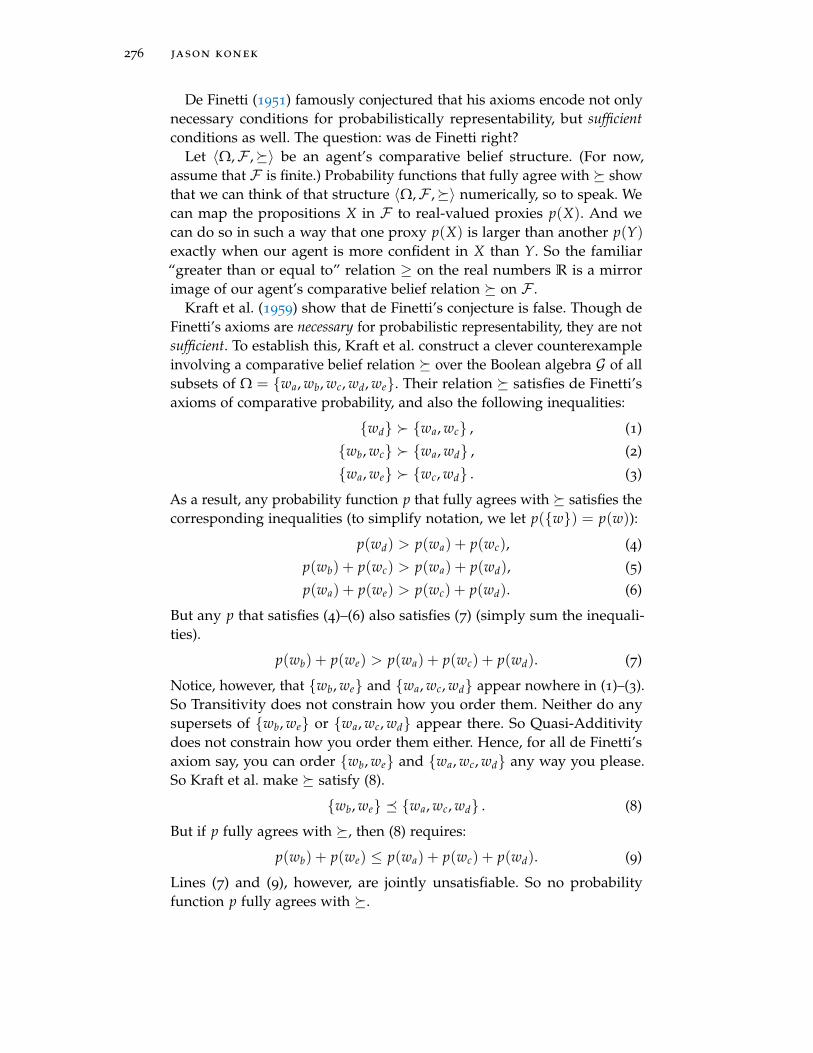
276 jason konek
De Finetti (1951) famously conjectured that his axioms encode not onlynecessary conditions for probabilistically representability, but sufficientconditions as well. The question: was de Finetti right?
Let 〈Ω,F ,〉 be an agent’s comparative belief structure. (For now,assume that F is finite.) Probability functions that fully agree with showthat we can think of that structure 〈Ω,F ,〉 numerically, so to speak. Wecan map the propositions X in F to real-valued proxies p(X). And wecan do so in such a way that one proxy p(X) is larger than another p(Y)exactly when our agent is more confident in X than Y. So the familiar“greater than or equal to” relation ≥ on the real numbers R is a mirrorimage of our agent’s comparative belief relation on F .
Kraft et al. (1959) show that de Finetti’s conjecture is false. Though deFinetti’s axioms are necessary for probabilistic representability, they are notsufficient. To establish this, Kraft et al. construct a clever counterexampleinvolving a comparative belief relation over the Boolean algebra G of allsubsets of Ω = wa, wb, wc, wd, we. Their relation satisfies de Finetti’saxioms of comparative probability, and also the following inequalities:
wd wa, wc , (1)
wb, wc wa, wd , (2)
wa, we wc, wd . (3)
As a result, any probability function p that fully agrees with satisfies thecorresponding inequalities (to simplify notation, we let p(w) = p(w)):
p(wd) > p(wa) + p(wc), (4)
p(wb) + p(wc) > p(wa) + p(wd), (5)
p(wa) + p(we) > p(wc) + p(wd). (6)
But any p that satisfies (4)–(6) also satisfies (7) (simply sum the inequali-ties).
p(wb) + p(we) > p(wa) + p(wc) + p(wd). (7)
Notice, however, that wb, we and wa, wc, wd appear nowhere in (1)–(3).So Transitivity does not constrain how you order them. Neither do anysupersets of wb, we or wa, wc, wd appear there. So Quasi-Additivitydoes not constrain how you order them either. Hence, for all de Finetti’saxiom say, you can order wb, we and wa, wc, wd any way you please.So Kraft et al. make satisfy (8).
wb, we wa, wc, wd . (8)
But if p fully agrees with , then (8) requires:
p(wb) + p(we) ≤ p(wa) + p(wc) + p(wd). (9)
Lines (7) and (9), however, are jointly unsatisfiable. So no probabilityfunction p fully agrees with .

comparative probabilities 277
2.1 Scott’s Theorem
So de Finetti’s conjecture is false. De Finetti’s axioms of comparative prob-ability are not necessary and sufficient for probabilistic representability.Luckily, Kraft et al. (1959) and Scott (1964) provide the requisite fix. Theyprovide stronger axioms that are both necessary and sufficient for prob-abilistic representability. Scott’s axioms are more straightforward, so wewill focus our attention on them.
Before stating Scott’s theorem, it is worth noting that our formulationabuses notation a bit. Expressions ‘Xi’ and ‘Yi’ refer both to propositionsin F , as well as their characteristic functions, i.e., functions that take thevalue 1 at worlds w where Xi (or Yi) is true (i.e., w ∈ Xi), and take thevalue 1 at worlds w′ where Xi is false (i.e., w′ 6∈ Xi). This will turn out tobe a helpful bit of sloppiness.
Scott (1964) proves the following:
Scott’s Theorem. Every comparative belief structure 〈Ω,F ,〉(with finite F ) has a probability function p : F → R that fullyagrees with in the sense that
X Y ⇔ p(X) ≥ p(Y)
if and only if satisfies the following axioms.
1. Non-triviality. Ω ∅.
2. Non-negativity. X ∅.
3. Totality. X Y or Y X.
4. Isovalence. If X1 + . . . + Xn = Y1 + . . . + Yn and Xi Yifor all i ≤ n, then Xi Yi for all i ≤ n as well.
Axiom 4—sometimes called Scott’s axiom, the Isovalence axiom, or the Finitecancellation axiom—is the one new axiom of the bunch. To see what itsays, note that X1(w) + . . . + Xn(w) counts the number of truths in the setX1, . . . , Xn at world w. Ditto for Y1(w) + . . . + Yn(w). So
X1 + . . . + Xn = Y1 + . . . + Yn
says that the two sets of propositions, X1, . . . , Xn and Y1, . . . , Yn, con-tain the same number of truths come what may, i.e., in every possible world.We call such sets of propositions isovalent.
In light of this, the Isovalence axiom says that if X1, . . . , Xn andY1, . . . , Yn are isovalent, then you cannot think that the Xis are uniformlymore plausible than the Yis. (“Uniformly more plausible” here means thatyou think that Xi is at least as plausible as Yi for all i, and that Xj is strictlymore plausible than Yj for some j.) After all, an equal number of the Xis

278 jason konek
and Yis are guaranteed to be true! So you can only think that the Xis areat least as plausible as the Yis across the board if you think that they areequally plausible.
But how exactly does Scott prove his representation theorem? It is worthwalking through the proof strategy informally. This will help interestedreaders dig through the mathematical minutia in Scott (1964).
Indeed, it will prove instructive to use Scott’s strategy to establishsomething slightly stronger than Scott’s theorem.
Generalised Scott’s Theorem (GST). For any comparative be-lief structure 〈Ω,F ,〉 with finite F and a comparative beliefrelation that satisfies
1. Non-triviality. Ω ∅,
2. Non-negativity. X ∅,
the following two conditions are equivalent.
3. Isovalence. If X1 + . . . + Xn = Y1 + . . . + Yn and Xi Yifor all i ≤ n, then Xi Yi for all i ≤ n as well.
4. Strong representability. there exists a probability func-tion p : F → R that strongly agrees with in the sensethat
(i) X Y ⇒ p(X) ≥ p(Y),
(ii) X Y ⇒ p(X) > p(Y).
Scott’s theorem, as we shall see at the end of Section 2, follows fairlystraightforwardly from GST. We prove the GST in the appendix.
The key insight required for proving GST is this. In the presence ofNon-triviality and Non-negativity, strong representability boils down tosorting almost desirable gambles from undesirable gambles.5 On top of this,Scott (1964) shows that sorting almost desirable from undesirable gamblesis equivalent to satisfying Isovalence.6 Figure 1 summarizes the situation.
Given Non-triviality and Non-negativity
Strong rep. ⇔ Sort gambles ⇔ Isovalence
Figure 1: Logical relations between properties of
5 For an accessible introduction to desirable gambles, see Walley (2000). See Quaeghebeur(2014) for more detail.
6 More carefully, Scott (1964) shows that for any comparative belief relation that satisfiesNon-triviality and Non-negativity, satisfying Isovalence is sufficient for sorting almostdesirable from undesirable gambles. Showing that it is necessary is straightforward. Seethe appendix for proof.

comparative probabilities 279
Gambles are measurable quantities G : Ω→ R. Say that a gamble G isalmost desirable relative to iff it is a non-negative linear combination ofalmost desirable components:
(X1 −Y1), . . . , (Xn −Yn).
And say that each component Xi − Yi is almost desirable iff Xi Yi.Gamble G is a non-negative linear combination of (X1−Y1), . . . , (Xn −Yn)
just in case:G = ∑
iλi(Xi −Yi)
for some λ1, . . . , λn ≥ 0.We call components Xi − Yi almost-desirable if Xi Yi because any
probability function p that strongly agrees with determines a non-negative expected value for Xi −Yi:
Xi Yi ⇒ p(Xi) ≥ p(Yi)
⇔ Ep[Xi] ≥ Ep[Xi]
⇔ Ep[Xi −Yi] ≥ 0.
So if we interpret those values as payoffs in utility, then p expects Xi −Yito be at least as good as the status quo (i.e., its expected utility is non-negative).
Likewise, we call G almost desirable if it is a non-negative linear combi-nation of almost-desirable components because any probability function pthat strongly agrees with determines a non-negative expected value forG:
Xi Yi for all i ⇒ Ep[Xi −Yi] ≥ 0 for all i
⇒ ∑i
λiEp[Xi −Yi] ≥ 0
⇔ Ep
[∑
iλi(Xi −Yi)
]≥ 0
⇔ Ep[G] ≥ 0.
Similar remarks apply to undesirable gambles. We call a gamble G∗ undesir-able relative to iff it is a convex combination of undesirable components
(X∗1 −Y∗1 ), . . . , (X∗n −Y∗n ),
so thatG∗ = ∑
iλ∗i (X∗i −Y∗i ).
for some λ∗1 , . . . , λ∗n ≥ 0 with ∑i λ∗i = 1. A component X∗i − Y∗i is unde-sirable iff X∗i ≺ Y∗i . The reason is the same as before. Any probability

280 jason konek
function that strongly agrees with determines a negative expected valuefor undesirable components, as well as convex combinations of undesirablecomponents.
Now say that sorts almost desirable gambles from undesirable ones iff thetwo sets of gambles are disjoint. That is, if
A =G | G is almost desirable rel. to
and
U =G∗ | G∗ is undesirable rel. to
,
then sorts almost desirable gambles from undesirable ones iff
A∩U = ∅.
If fails to sort gambles in this way, then some gamble is both almostdesirable and undesirable, i.e., G = G∗ for some almost desirable gambleG and some undesirable gamble G∗. And if that is the case, then there is noprobability that strongly agrees with it. (Moreover, since full probabilisticrepresentability entails strong representability, there is no probabilityfunction that fully agrees with it either.) If it were strongly representable,then we would have both
Ep[G] = Ep[G∗]
andEp[G∗] < 0 ≤ Ep[G]
for some probability function p.This shows that sorting almost desirable from undesirable gambles is
necessary for strong agreement with a probability function, which is itselfnecessary for full agreement with a probability function, i.e., probabilisticrepresentability. Scott’s insight, though, is that it is also sufficient, in thepresence of Non-triviality and Non-negativity. Given that satisfies Non-triviality and Non-negativity, it sorts almost desirable from undesirablegambles if and only if it strongly agrees with a probability function. What’smore, if is total as well, then strong agreement is equivalent to fullagreement. So non-trivial, non-negative, total comparative belief relationssort almost desirable from undesirable gambles if and only if they areprobabilistically representable. See Figure 2.
To prove this, Scott uses what is known as a hyperplane separation theorem.The hyperplane separation theorem guarantees that for any two closed,convex, disjoint sets, there is a hyperplane that strictly separates them(Kuhn & Tucker, 1956, p. 50). Now note that A is the closed, convexpolyhedral cone generated by the set
X−Y | X Y
. Likewise, U is the
convex hull of
Y− X | X Y
—a closed and convex set. And if sorts

comparative probabilities 281
Given Non-triviality, Non-negativity and Totality
Strong rep. ⇔ Full prob. rep.m
Sort gambles ⇔ Isovalence
Figure 2: Logical relations between properties of
−1 0 1−1
0
1
A
U
Figure 3: Hyperplane strictly separating A and U
almost desirable from undesirable gambles, then they are also disjoint. Sothere is a hyperplane that strictly separates A and U (see Figure 3).
This hyperplane determines (in effect) an expectation operator E. Gam-bles G on one side of the hyperplane get positive expected values accordingto E. Gambles on the other side get negatives ones. Precisely how high orlow E[G] happens to be is determined by G’s distance from the hyperplane.
The resulting expectation operator E assigns a non-negative value toevery almost desirable gamble G in A, and a negative value to everyundesirable gamble G∗ in U:
E[G] ≥ 0 for all G ∈ A,
E[G∗] < 0 for all G∗ ∈ U.

282 jason konek
And from this expectation operator, E, it is fairly straightforward to extracta probability function p that strongly agrees with . Just let p(X) = E[X]
for all X ∈ F .7 Then we have:
Xi Yi ⇒ E[Xi −Yi] ≥ 0
⇔ E[Xi] ≥ E[Yi]
⇔ p(Xi) ≥ p(Yi).
We also have:
X∗i ≺ Y∗i ⇒ E[X∗i −Y∗i ] < 0
⇔ E[X∗i ] < E[Y∗i ]
⇔ p(X∗i ) < p(Y∗i ).
The upshot: sorting almost desirable from undesirable gambles is bothnecessary and sufficient for strong agreement with a probability function(in the presence of Non-triviality and Non-negativity).
Now for the kicker: a comparative belief relation —whether or not itsatisfies Non-triviality and Non-negativity—sorts almost desirable fromundesirable gambles (in the sense that A ∩U = ∅) if and only if itsatisfies Isovalence.8 Hence non-trivial and non-negative are stronglyrepresentable if and only if they satisfy Isovalence. What’s more, as wementioned above, for total comparative belief relations it’s easy to seethat strong agreement with a probability function is equivalent to fullagreement. So non-trivial, non-negative, total are fully probabilisticallyrepresentable if and only if they satisfy Isovalence. This is the main thrustof Scott’s theorem.
2.2 Varieties of Representability
There are, of course, other types of representability besides just strong andfull probabilistic representability. For example, a probability function pstrongly agrees with just in case it satisfies two conditions:
X Y ⇒ p(X) ≥ p(Y),
X Y ⇒ p(X) > p(Y).
7 More methodically, the hyperplane separation theorem gives a strictly separating linearfunctional, φ. But given that satisfies Non-triviality and Non-negativity, A and U havea certain structure, which guarantees that we can normalise φ to arrive at an expectationoperator E. For example, Non-triviality ensures that ∅ − Ω ∈ Y . Hence φ(Ω) > 0.Normalising then gives us E[Ω] = 1. Similarly, Non-negativity ensures that X −∅ ∈ X .Hence φ(X) ≥ 0, and in turn E[X] ≥ 0.
8 See Scott (1964, pp. 235–6) for the proof of sufficiency. We present a simplified version ofboth necessity and sufficiency in the appendix.

comparative probabilities 283
We can pick apart these two conditions to arrive at two weaker notions ofrepresentability. Say that
p almost agrees with iff
X Y ⇒ p(X) ≥ p(Y),
and also that
p partially agrees with iff
X Y ⇒ p(X) > p(Y).
A comparative belief relation is almost representable if there is a proba-bility function p that almost agrees with . Likewise, is partially rep-resentable if there is a probability function p that partially agrees with.
Kraft et al. (1959) show that is almost representable if and only if itsatisfies the Almost-Cancellation axiom.
Almost-Cancellation. If
X1 + . . . + Xn < Y1 + . . . + Yn
and Xi Yi for all i 6= j, then Xj 6 Yj.
Similarly, Adams (1965) and Fishburn (1969) show that is partiallyrepresentable if and only if it satisfies the Partial-Cancellation axiom.
Partial-Cancellation. If X1 + . . . + Xn ≤ Y1 + . . . + Yn andXi Yi for all i 6= j, then Xj 6 Yj.
It does not, to be clear, follow from these two results that is stronglyrepresentable if and only if satisfies both the Almost and Partial-Cancellation axioms. Satisfying Almost and Partial-Cancellation wouldsimply guarantee that (i) some probability function p almost agrees with, and (ii) some possibly distinct probability function q partially agreeswith . But strong representability requires that a single probability func-tion do both types of agreeing. It is an open question what exactly isrequired for strong representability. (Of course, GST identifies necessaryand sufficient conditions for strong representability given Non-triviality andNon-negativity. But clearly neither of those conditions is itself necessaryfor strong representability.)
Almost, partial, and strong representability all place negative demandson your comparative beliefs. They require you to avoid certain sets ofcomparative beliefs. Say that
p endorses iff p(X) ≥ p(Y)⇒ X Y.

284 jason konek
For your comparative belief relation to be almost representable, youmust avoid having weak comparative beliefs that no probability functionwhatsoever endorses. Likewise, for to be partially representable, youmust avoid having strict comparative beliefs that no probability functionendorses. For to be strongly representable, you must avoid both.
Full probabilistic representability is stronger. It makes positive demandsas well as negative demands on your comparative beliefs. Full probabilisticrepresentability requires your comparative beliefs to be sufficiently richand specific that some probability function endorses exactly those compar-ative beliefs. So not only must you avoid comparative beliefs that are notendorsed by any probability function, but you must positively go in for allof the comparative beliefs endorsed by some probability function.
Imprecise representability, or IP-representability, strikes a balance betweenthese previous types. Like strong representability, IP-representabilityplaces negative demands on your comparative beliefs. It requires you toavoid comparative beliefs that no probability function endorses. But likefull probabilistic representability, it also makes positive demands on yourcomparative beliefs. It does not go so far as to demand that you go in forall of the comparative beliefs endorsed by some probability function. Butit does say that you must already be more confident in X than Y if everyprobability function that endorses your other comparative beliefs endorsesX Y as well. In this way, it requires you to draw out the “probabilisticconsequences” of your other comparative beliefs.
Formally, a comparative belief relation is imprecisely representable ifand only if there is a set of probability functions P that fully agrees withit:
P fully agrees with iff
X Y ⇔ p(X) ≥ p(Y) for all p ∈ P .
Rios Insua (1992) and Alon and Lehrer (2014) show that is IP-representable if and only if it satisfies Reflexivity, Non-negativity, Non-triviality, and the Generalised Finite-Cancellation axiom.
Generalised Finite-Cancellation axiom. If
X1 + . . . + Xn + A + . . . + A︸ ︷︷ ︸k times
= Y1 + . . . + Yn + B + . . . + B︸ ︷︷ ︸k times
and Xi Yi for all i ≤ n, then A B.
IP-representability is clearly stronger than strong representability.IP-representability implies strong-representability. But a strongly repre-sentable comparative belief relation might fail to satisfy Reflexivity,Non-negativity, and Non-triviality. No IP-representable will do so,

comparative probabilities 285
Full prob. rep.
Imprecise rep.
Strong rep.
Partial rep.Almost rep.
Figure 4: Logical relations between different types of representability
however. So strong-representability does not imply IP-representability.Moreover, Harrison-Trainor, Holliday, and Icard (2016) show that even fornon-trivial, non-negative, and reflexive , IP-representability is strongerthan strong representability.
To wrap up, let’s taxonimise these various types of representabilityaccording to their logical strength: see Figure 4.
2.3 Loose Ends: Infinite Algebras, Conditional Comparative Beliefs, Etc.
Scott (1964, p. 247) claims that his theorem extends to comparative beliefstructures 〈Ω,F ,〉 with infinite algebras F , by a clever application of theHahn-Banach Theorem. The proof however remains unpublished. Suppesand Zanotti (1976) also provide necessary and sufficient conditions for acomparative belief relation on an infinite algebra to be fully probabilisti-cally representable. Suppes and Zanotti’s axioms, however, do not directlyconstrain comparative beliefs. Rather, they show that is probabilisticallyrepresentable if and only if it is extendable to a comparative estimation rela-tion over a larger set; a set containing not just propositions—sets of worlds,or equivalently, functions from worlds to 1 (true) or 0 (false), i.e., indicatorfunctions—but to real-valued quantities Q : Ω→ R more generally.
To get the rough idea, consider a travel agent. She might not havea precise estimate of how many travelers will go to Hawaii this year.(Perhaps her evidence is incomplete and ambiguous.) Likewise, she mightnot have a precise estimate of how many travelers will go to Acapulco.Despite this, she might well estimate that more travelers will go to Hawaiithan Acapulco. Or consider the weather. Alayna might not have a preciseestimate of how much rain London will receive in June. She might nothave a precise estimate of how much rain Canterbury will receive in June.Despite this, she might estimate that London will receive more rain thanCanterbury.
Ditto for stock prices, or the number of MPs that different parties willlose or gain in the next election, or any other quantity you might care about.You can have comparative estimates regarding those respective quantities—i.e., estimate that one quantity Q will have a higher/equal/lower value

286 jason konek
than another quantity Q∗—without having a unique, precise best estimatefor any of them.
Call a relation ∗ on a set F ∗ of real-valued quantities defined on Ωa comparative estimation relation if it is used to model an agent’s compara-tive estimates. And call a comparative estimation relation ∗ qualitativelysatisfactory if it satisfies the following (putative) coherence constraints.
1. ∗ is transitive and total.
2. Ω ∗ ∅.
3. X ∗ ∅.
4. X ∗ Y iff X + Z ∗ Y + Z.
5. If X ∗ Y then for all W, Z ∈ F ∗, there’s an n > 0 such that
X + . . . + X︸ ︷︷ ︸n times
+W ∗ Y + . . . + Y︸ ︷︷ ︸n times
+Z.
Suppes and Zanotti (1976) show that a comparative belief relation onan algebra F of propositions (indicator functions), whether F is finiteor infinite, is fully probabilistically representable if and only if there is acomparative estimation relation ∗ on the set F ∗ of non-negative integer-valued quantities
F ∗ =Q | Q : Ω→ Z≥0
,
which both (i) extends , and (ii) is qualitatively satisfactory.This shows that whatever latent structural defect prevents a comparative
belief relation from being fully probabilistically representable rears itshead explicitly when you extend the relation. If has this defect, thenwhen you extend it, so that it encodes not just comparative estimates oftruth-values of propositions, but also comparative estimates of the valuesof non-negative integer-valued quantities more generally, what you end upwith—your new, larger comparative estimation relation ∗—will violateone of Suppes and Zanotti’s putative coherence constraints. And vice versa.If does not have this latent defect, then there is some way of extending itthat does not violate those constraints.9
Of course, the representation theorems surveyed here are just the tipof the iceberg. For example, we said that a comparative belief relation is imprecisely representable if and only if there is a set of probabilityfunctions P that fully agrees with it. But we could explore full agreement(or almost agreement, or partial agreement, or strong agreement) with any
9 Suppes and Zanotti’s axiom 5 is an “Archimedean axiom,” which guarantees (roughly)that differences in one’s best estimates are not “infinitely small.” For a non-Archimedeantheory of comparative estimation, see Pederson (2014).

comparative probabilities 287
number of imprecise probability models: Dempster-Shafer belief functions,n-monotone Choquet capacities, coherent lower previsions/expectations,or coherent lower probabilities (cf. Walley, 1991, 2000; Augustin, Coolen,de Cooman, and Troffaes, 2014; Troffaes and de Cooman, 2014).
Alternatively, we could focus not on comparative belief relations, butconditional comparative belief relations. Hájek (2003)—following Rényi(1955), Jeffreys (1961), de Finetti (1974), and others—argues forcefullythat we should treat precise conditional credence as more fundamentalthan precise unconditional credence. Similarly, we might treat conditionalcomparative beliefs of the form
A | B C | D
as more fundamental than unconditional comparative beliefs. A | B C |Dsays that the agent in question is at least as confident in A given B as sheis in C given D. We can then recover unconditional comparative beliefrelations from comparative ones by conditioning on the tautology, Ω:
A B⇔ A |Ω B |Ω.
Say that a conditional comparative belief relation on F is probabilisti-cally representable if there is a conditional probability function that fullyagrees with it. More carefully: there is a probability function p : F → R
such that for any two propositions A, B ∈ F , and any two non-null propo-sitions C, D ∈ F , we have
A | B C | D ⇔ p(A ∩ B)p(B)
≥ p(C ∩ D)
p(D).
A proposition X is non-null just in case it is not just as likely as thecontradiction, i.e.,
X |Ω 6≈ ∅ |Ω.
Now we can ask: when are conditional comparative belief relations prob-abilistically representable? Domotor (1969) extends the results of Scott(1964) to provide necessary and sufficient conditions for probabilistic rep-resentability when is defined on a finite algebra F . Suppes and Zanotti(1982) extend the results of Suppes and Zanotti (1976) to provide necessaryand sufficient conditions in the general case (whether or not F is finite).See Suppes (1994) for additional detail.
With a basic understanding of representation theorems and their me-chanics in hand, we can now turn our attention to the central question ofthis chapter: do comparative beliefs and representation theorems figureinto the best explanation of what precise credences are? If so, how? Whatdo these accounts of credence look like? And how do they stand up to thecriticisms of Hájek (2009), Meacham and Weisberg (2011), and Titelbaum(2015)?

288 jason konek
3 the comparative belief-credence connection
To a first approximation, an agent’s credence function measures howconfident she can be said to be in each proposition. If c(X) = 1, then she ismaximally confident that X is true, i.e., 100% confident. If c(X) = 0, thenshe is minimally confident that X is true, i.e., 0% confident. If c(X) = 2/3,then she is more confident than not that X is true, but not quite fullyconfident.
But what does this really mean? What does it mean to say that an agentis 100%, or 80%, or 23.9556334% confident in a proposition?
We might have similar questions for imprecise Bayesians. ImpreciseBayesians model rational agents’ opinions not with a single credencefunction c, but with a set of credence functions C. Sets of credence func-tions are called imprecise credal states (see Mahtani, this volume).10 To afirst approximation, imprecise credal states also measure how confidentagents can be said to be in various propositions. But they allow for astrictly greater range of opinions than precise credal states. For example,if c(X) = 1 for all c in C, then our agent is 100% confident that X is true.If, however, 0.6 ≤ c(X) ≤ 0.9 for all c in C, and nothing stronger, then sheis at least 60% confident and at most 90% confident that X is true. But shehas no precise level of confidence for X. Precise credence functions allowfor the first sort of opinion, but not the second.
But again, what exactly does this mean? What does it mean to saythat an agent is at least 60% confident and at most 90% confident in aproposition?
The history of Bayesianism is chock-full of different accounts of credencethat aim to answer this question. Very roughly, we can lump them intothree groups: measurement-theoretic accounts, decision-theoretic accounts,and interpretivist accounts. Before exploring the differences between thesevarious accounts, it is worth emphasising one similarity. They all treat‘credence function’ or ‘credal state’ in roughly the way Carnap treatedtheoretical terms more generally. They carve out some theoretical role (orset of roles) R as constitutive of what it is for a real-valued function, c, ora set of such functions, C, to count as “your credal state.” The better c (orC) plays role R, the more eligible it is as a “credal state candidate.” Whatthese accounts disagree on is what the relevant theoretical role R is.
10 Precise credal states are special cases of imprecise credal states, on the imprecise Bayesianview. Formally, C is precise just in case C = c for some credence function c.

comparative probabilities 289
3.1 Measurement-Theoretic Account of Credence
Measurement-theoretic accounts, like those of Koopman (1940a, 1940b), Good(1950), and Krantz et al. (1971), treat credal states as mere numerical mea-surement systems for comparative beliefs (or more generally, for someunderlying structure of comparative and qualitative opinions). Compare:numerical measurement systems for length, mass, velocity, etc., allowengineers, scientists and the like to measure certain parts of the systemof interest, perform numerical calculations, and draw inferences aboutother parts of the system. Imagine, for example, measuring the length oftwo pieces of wood arranged at a right angle, and using the Pythagoreantheorem to infer how long the diagonal must be.
Similarly, on the measurement-theoretic view, credal states are merenumerical measurement systems. They allow you to measure certainparts of an agent’s system of comparative beliefs, perform numericalcalculations, and draw conclusions about what other comparative beliefsshe must have (or must not have). Imagine, for example, that you elicit asufficient number of an agent’s comparative beliefs to be quite confidentthat (i) she satisfies Scott’s axioms, so that fully agrees with someprobability function c, and further that (ii) c(X) = 0.3, c(Y) = 0.4, andc(X ∩ Z) = c(Y ∩ Z) = 0. Given these measurements, you can use theprobability axioms to calculate that c(X ∪ Z) ≤ c(Y ∪ Z). Since c fullyagrees with , you can infer that X ∪ Z Y ∪ Z. (See Section 5 for a morecomplete introduction to the measurement-theoretic view.)
The upshot: just like measurement systems for physical quantities(length, etc.), credal states allow you to represent comparative beliefsin an elegant, easy-to-use, numerical fashion. And modeling comparative(and qualitative) beliefs with numbers is useful. Numerical measurementsystems are designed specifically to reflect important structural featuresof the underlying target system, so that you can use them to straightfor-wardly extract information about one part of the system from informationabout other parts.
Where does this leave us? The measurement-theoretic view takes aparticular stand on the nature of the theoretical role R that a function c(or set of functions C) must play in order to count as “your credal state.”More specifically, c (or C) must fully agree (or almost agree, or partiallyagree, or strongly agree) with the agent’s comparative beliefs, , in theway required to count as a numerical measurement system for . Thebetter c (or C) plays this role R, the more eligible it is as a credal statecandidate. Equally good measurement systems are equally eligible credalstate candidates.

290 jason konek
3.2 Decision-Theoretic Account of Credence
Decision-theoretic accounts of credence, like those of Ramsey (1931), de Finetti(1931, 1964), and Walley (1991), carve out a rather different theoreticalrole for credal states. Credal states, on these views, encode an agent’s fairbuying and selling prices. An agent’s fair buying price for a gamble G is,roughly, the largest amount that she could pay for G while still leavingherself (in her own view) in at least as good a position as the status quo.An agent’s fair selling price for a gamble G is, roughly, the smallest amountthat someone else would have to pay her in exchange for G in order toleave herself (in her own view) in at least as good a position as the statusquo.
To illustrate, imagine that you have an urn. The urn contains 10 balls.Each ball is either red or black. There are at least 3 black balls, and at most7 black balls. But you have no absolutely no idea whether the urn contains3, 4, 5, 6, or 7 black balls.
Let G be the gamble that pays out £10 if a random draw from the urnyields a black, and £0 otherwise. Given what you know about the contentsof the urn, you would likely judge that paying a measly £1 for G is a gooddeal. Maybe £2 is a good deal too. But let’s imagine that £3 is your limit.Paying any more than £3 would leave you in a situation where you areno longer, in your own view, determinately doing at least as well as thestatus quo. Then your fair buying price for G is 3. More carefully, your fairbuying price for G is 3 iff you weakly prefer paying 3 and receiving G tothe status quo, but not so for any amount higher than 3.
Similarly, suppose that a friend wants to buy G from you. They willpay you some initial amount. Then you will pay them £10 if the drawcomes up black and £0 otherwise. Given what you know about the urn,you would likely judge that selling G to your friend for £9 is a good deal(for you, anyway). Maybe £8 is a good deal too. But let’s imagine that £7is your limit. If they offer you any less than £7, then you would be leftin a position where you are no longer, in your own view, determinatelydoing at least as well as the status quo. Then your fair selling price for Gis 7. More carefully, your fair selling price for G is 7 iff you weakly preferreceiving 7 and selling G to the status quo, but not so for any amountlower than 7.
On the decision-theoretic view, the principal theoretical role of an agent’scredal state is to encode her fair buying and selling prices. A set E of real-valued functions e counts as “your credal state” just in case its lower andupper envelope for gambles G,
E [G] = inf
e(G) | e ∈ E
,
E [G] = sup
e(G) | e ∈ E
,

comparative probabilities 291
are equal to your fair buying and selling prices for G, B(G) and S(G),respectively, i.e., E [G] = B(G) and E [G] = S(G). (Treat a single real-valuedfunction e as the singleton E = e.) The better E plays this role R—thecloser its lower and upper envelopes are to your fair buying and sellingprices—the more eligible it is as a credal state candidate.
Your credal state only captures information about your beliefs, on thisview, insofar as they are reflected in your fair buying and selling prices.For any proposition X ∈ F , let GX be the unit gamble on X, i.e., the gamblethat pays out £1 if X and £0 otherwise. Your lower and upper “previsions”for GX, E [GX] and E [GX] (i.e., the value of the lower and upper envelopesof E at GX), encode your fair buying and selling prices for GX. If you arewilling to pay something near £1 for a unit gamble on X (E [GX] ≈ 1),then for the purposes of decision-making you are quite confident in X. If youwould be happy to sell a unit gamble on X to a friend for mere pennies(E [GX] ≈ 0), then for the purposes of decision-making you have extremelylow confidence in X. If you would only buy a unit gamble on X for next tonothing (E [GX] ≈ 0), and would only sell a unit gamble on for close to itsmaximum payout (E [GX] ≈ 1), then for the purposes of decision-makingyou have no idea whether X is true. Your opinions are rather imprecise.
The decision-theoretic view comes in many flavours—one for each wayof thinking about the preferences that determine your fair buying andselling prices. On a flat-footed behaviourist view, B(G) is your fair buyingprice for G just in case you actually buy G for B(G), and actually refuse tobuy G for any higher price (or perhaps do so a sufficiently high proportionof the time). On a more sophisticated behaviourist view, B(G) is your fairbuying price for G just in case you are disposed to buy G for B(G), anddisposed to refuse to buy G for any higher price. Alternatively, we mightreject behaviourism in its various guises, and say that the preferences thatfix your fair buying/selling prices are irreducibly evaluative attitudes.
But where do comparative beliefs enter the picture? It may not appearthat comparative beliefs play an especially important role in explicatingthe concept of credence on the decision-theoretic view. After all, on thisview, an agent’s credal state encodes her fair buying and selling prices.And fair buying and selling prices are fixed by one’s preferences, nottheir comparative beliefs. Even on Savage’s view, where comparative beliefreduces to preference, different fragments of an agent’s preference relationfix her fair buying/selling prices and comparative beliefs, respectively.Nonetheless, rational comparative beliefs and fair buying/selling priceshang together in a certain way (Section 6). So comparative beliefs (andrepresentation theorems) will be important for answering the normativequestion, even on the decision-theoretic view.
Also worth noting: if an agent has a precise credal state E = e, then
E [G] = E [G]

292 jason konek
for all gambles G. That is, her fair buying prices just are her fair sellingprices. The maximum amount she is willing to pay for G is precisely theminimum amount she is willing to accept in exchange for selling G. Agentswith genuinely imprecise credal states (non-singleton E ), in contrast, maywell think that buying is worthwhile only at very low prices, and selling isworthwhile only at very high prices. Imprecise Bayesians typically see thisas the proper (or at least a permissible) type of evaluative attitude to bear indecision contexts where evidence is unspecific or ambiguous.
One final note: measurement-theoretic and decision-theoretic accountsof credence can be difficult to distinguish in practice. Consider a propo-nent of the measurement-theoretic account, such as Savage, who treatscomparative belief as reducible to preference (Savage, 1954, Section 3.2).You judge that X Y iff whenever you prefer one outcome to another, youalso prefer getting the better outcome if X than if Y. Then certain typesof measurement systems for comparative belief—viz., sets of probabilityfunctions—encode fair buying and selling prices (see Section 6). Whencethe difference, then, between this sort of measurement-theoretic accountof credence, and a decision-theoretic account?
The difference is this. On the measurement-theoretic view, any numericalmeasurement system for does the work necessary to count as “yourcredal state”—not just ones that encode your fair buying and sellingprices. Likewise, on the decision-theoretic view, any numerical system thatencodes your buying and selling prices counts as “your credal state.” Butsome of those systems (viz. upper and lower previsions) carry too littleinformation to determine a numerical representation of your preferencerelation (Walley, 2000, Section 6).
Shorter: even though some numerical systems do both jobs (measu-rement-theoretic and decision-theoretic), it is possible to do one withoutdoing the other. So the two accounts make different predictions aboutwhich functions (sets of functions) count as “eligible credal state candi-dates.”
3.3 Interpretivist Account of Credence
Our final account of credence is the interpretivist account, of the sort es-poused by Lewis (1974) and Maher (1993). According to preference-basedinterpretivist accounts, like Patrick Maher’s, “an attribution of probabili-ties and utilities is correct just in case it is part of an overall interpretationof the person’s preferences that makes sufficiently good sense of themand better sense than any competing interpretation does” (Maher, 1993, p.12). And according to Maher, if some probabilistically coherent credencefunction c and cardinal utility function u jointly agree with an agent A’spreferences, in the following sense:

comparative probabilities 293
A weakly prefers α to β
iffEc[α] ≥ Ec[β]
(where Ec[α] and Ec[β] are the expected utilities of acts α and β relative toc and u, respectively), then c and u perfectly rationalise or make sense of thatagent’s preferences.
On Maher’s view, both credence functions and utility functions earntheir theoretical keep by rationalising preferences. If c and u rationaliseyour preferences better than any competing c∗ and u∗, then c plays theappropriate theoretical role to count as “your credal state,” and u playsthe appropriate theoretical role to count as “your utility function.” Thispresupposes the thesis of the primacy of practical reason. Whether ornot c rationalises your comparative and qualitative beliefs, understood asirreducibly doxastic attitudes, is neither here nor there. What makes c “yourcredence function” is the fact that it helps to rationalise your preferences.
But we can distinguish another brand of interpretivism: epistemic inter-pretivism. This is a new account of credence. So we will spend a bit of timedeveloping it.
According to epistemic interpretivism, credal states are assignments oftruth-value estimates (or sets of such assignments) that rationalise one’scomparative beliefs (or more generally, her comparative and qualitativeopinions), understood as irreducibly doxastic attitudes. A function c :F → R (or set C) counts as “your credal state” just in case it encodes truth-value estimates (or constraints on such estimates) that best rationalise ormake sense of your comparative beliefs.
Spelling out epistemic interpretivism requires two things: (i) sayingsomething about what truth-value estimates are, and (ii) explaining whatit means for truth-value estimates to best rationalise a set of comparativebeliefs.
Estimates are familiar enough. For example, an analyst’s best estimateof Tesla’s stock price 1 years hence might be $425. Your best estimate ofthe number of bananas in a randomly selected bunch might be 5.7. And soon. In each of these examples, there is the agent doing the estimating, thereis the quantity being estimated, and there is the estimate of that quantity.For the purposes of spelling out epistemic interpretivism, it is the last ofthese that matters most.
Estimates are numbers. But not all numbers are estimates. For example,the numbers in the expression
1, 000, 000 > 2
are not estimates. What sorts of numbers are estimates then? Plausibly,they are numbers that are subject to a certain standard of evaluation. A

294 jason konek
number is an estimate in a context iff it is evaluated qua estimate in thatcontext. In typical contexts of evaluation, numbers like 2 in expressions likethe above are not estimates because they are not evaluated qua estimates.There is no quantity that it would be better or worse for 2 to be close to. Itis no better or worse for being close to the actual price of stock X, or theactual dosage of drug Y, etc. In contrast, the number at the bottom of acontractor’s quote—a paradigm of an estimate—is evaluated qua estimate.It is quite bad, for example, if it is £20, 000 off the actual price of the job.
What exactly is it to evaluate a number qua estimate? We will not providea full answer here. But we can say something informative.
The type of phenomenon under consideration—evaluating an entity Equa X—is a common one. You might be brilliant qua scientist, mediocrequa mentor, and terrible qua conversationalist. The reason seems to bethis: scientists, mentors and conversationalists all perform characteristicfunctions. And you can perform some functions well while performingothers poorly. Microbiologists, for example, carefully dissect tissue samples,meticulously document their experiments, write up academic papers,communicate their results at conferences, etc. Conversationalists, on theother hand, ask engaging questions, are familiar with current events, andso on. You might well dissect tissue samples masterfully, but have no ideawhat the news of the day is.
This suggests the following. Evaluating an entity E in some capacity X , orqua X , is a matter of evaluating E on the basis of how well it performs thecharacteristic functions F1, . . . ,Fn associated with X . What to say aboutestimates in particular then? What characteristic functions do they serve,for example, in scientific inquiry, engineering, finance, etc.? Whatever thefull answer is, the following seems non-negotiable: an estimate of quantityQ serves the function of approximating the true value of Q. So ceterisparibus it is better the closer it is to the true value of Q.
Note that, on the present account, for a number to count as an estimate ina context, there must be an evaluator in that context; an agent evaluating thenumber qua estimate. (This need not require having the concept estimate,or anything of the sort. Evaluating a number qua estimate might be a fairlycognitively undemanding task.) But there need be no estimator; no agentproducing the estimate; no agent explicitly judging that this is the bestestimate of that, etc.
Thermometers provide estimates of temperature. Geiger counters pro-vide estimates of radiation. Ditto for other measurement devices. In eachof these cases, there is an estimate (38C, 0.10mSv, etc.), but no estimator;no agent doing the estimating. Similarly, a tree’s rings provide an estimateof its age. Your parents’ income provides an estimate of your income.Again, estimates without estimators. And estimates, of course, do not needto be good. The number of tea leaves concentrated in one part of your cup

comparative probabilities 295
provides a (thoroughly unreliable) estimate of the number of fortunateevents in your future. Once more: estimate, but no estimator.
The upshot: we can talk of estimates doing this or that—for example,rationalising a set of comparative beliefs—even if those estimates do not“belong” to anyone. Estimates without estimators.
Back to our original question: what are truth-value estimates? We havemade some progress in saying what estimates are more generally. Now,following de Finetti and Jeffrey, treat a proposition X as an “indicatorvariable” that takes the value 1 at worlds where X is true, and 0 where Xis false. Truth-value estimates, then, are simply estimates of the value, 0 or1, that the proposition takes at the actual world.
To finish spelling out the epistemic interpretivist account of credence, weneed to explain what it means for truth-value estimates to “best rationalise”a set of comparative beliefs. To get a feel for how this might work, consideran example. Grandma relies on folklore methods for predicting the weather.She feels things in her bones, observes the behaviour of the cows in thepasture, etc. You are not sure whether the weather-related opinions thatGrandma comes to on this basis make much sense or not. But then youopen your weather app. Lo and behold, you find a bunch of estimates—probabilities for sun, clouds, rain, etc., estimates of rainfall amount, hour-by-hour temperature estimates, etc.—that recommend thinking preciselywhat Grandma thinks. For example, Grandma thinks it is likelier than notto rain this evening. And the weather app recommends thinking that too.It specifies a greater than 50% probability of rain. (We will explore a fewdifferent accounts of recommendation shortly.)
The weather app’s estimates recommend having Grandma’s opinions.And these estimates are themselves eminently rational. In virtue of this,they rationalise or make sense of those opinions.
Note, however, that the weather app itself is not essential to this story.Estimates do not need an estimator. If there exists some rational set ofestimates that recommend Grandma’s opinions, then whether or notany weather app actually spits those estimates out, or any meteorologistactually judges those estimates to be best—or indeed whether any artificialor human system is in the business of explicitly estimating quantitiesat all—Grandma’s opinions are nonetheless rationalisable. The rationalestimates that recommend her opinions provide that rationale.
Before saying something more general about when a set of truth-valueestimates best rationalises a set of comparative beliefs, we should keyin on two important features of our example. The first is the strengthof the recommendation in question. The second is the quality of thatrecommendation.
We stipulated that the weather app’s estimates recommend havingGrandma’s opinions. This makes it seem as though recommendation is

296 jason konek
an on-off matter. But recommendations plausibly come in degrees. Youcan recommend a trip to the Alps a little more strongly than a trip toTahoe, but much more strongly than a trip to Cudahy, Wisconsin. In ourexample, the weather app’s estimates most strongly recommend thinkingprecisely what Grandma thinks. We might have stipulated, however, thatthey recommend a similar but distinct state of opinion most strongly, andrecommend Grandma’s state of opinion a little less strongly. In that case,the weather app’s estimates provide a fairly strong, but not maximallystrong rationale for Grandma’s state of opinion.
In addition to the strength of a recommendation, we can consider thequality of that recommendation. We stipulated that the weather app’sestimates are eminently rational. But our weather app could have been abit glitchy and delivered mildly irrational estimates (ones that violate theprobability axioms, perhaps, but not by much). Those estimates might stillrecommend thinking what Grandma thinks just as strongly. But in virtueof their mild irrationality, they provide a slight lower quality rationale forGrandma’s state of opinion.
The distinction between strength and quality is important. If Grandma’sstate of opinion is epistemically defective, it may turn out that no estimatesunreservedly recommend it, i.e., recommend it at least as strongly as anyother state of opinion. Every set of estimates might recommend some otherstate of opinion more strongly. Nonetheless, some sets of estimates mightrecommend Grandma’s state of opinion more strongly than others. Andamongst the sets of estimates that recommend it as strongly as possible(at least as strongly as any other set of estimates), some might provide ahigher quality recommendation than others. The extent to which a set ofestimates rationalises or makes sense of a state of opinion depends on bothstrength and quality. To provide the best possible rationale for Grandma’sstate of opinion, for example, a set of estimates must (i) recommendthat state as strongly as possible, and (ii) must provide the highest qualityrecommendation from amongst the sets of estimates that satisfy (i).
Let’s take stock. According to epistemic interpretivism, a function c :F → R (or set of functions C) counts as “your credal state” just in caseit encodes truth-value estimates (or constraints on such estimates) thatbest rationalise or make sense of your comparative beliefs. We gave a briefaccount of estimatehood to fill this out a bit. And we quickly unpackedwhat it means for c (or C) to “best rationalise” your comparative beliefs,. To best rationalise , c should provide at least as strong a rationale for as any other set of truth-value estimates c∗. And on the picture sketchedabove, c provides a rationale for by recommending . So for c to countas “your credal state,” no other c∗ can recommend more strongly thanc. Moreover, amongst the truth-value estimates that provide a maximallystrong rationale for (recommend it as strongly as possible), c should

comparative probabilities 297
provide at least as high quality a rationale as any other c∗. On the picturesketched above, the quality of c’s rationale depends on how close c itselfis to rational. So for c to count as “your credal state,” no other c∗ thatrecommends as strongly as possible should be more rational than c.Pulling this all together, c (or C) counts as “your credal state” just in caseit encodes truth-value estimates (or constraints on such estimates) thatrecommend your comparative beliefs as strongly as possible, and are asrational as possible whilst doing so. See Figure 5.
c1 c2 c3
Estimates that recom-mend your compara-tive beliefs as stronglyas possible
Maximallyrationalestimates
Provides somerationale foryourcomparative be-liefs
Provides ahigher qualityrationale
Provides thehighest qualityrationale
Figure 5: More rational estimates provide higher quality rationales.
The big lingering question is this: when exactly does a set of truth-value estimates recommend a certain set of comparative beliefs more or lessstrongly? There are a number of ways one could spell this out. We will notdefend a particular account of recommendation here. But here are threeoptions.
Metaphysical Account. The truth-value estimates given byc : F → R recommend to degree k iff it is metaphysicallynecessary that any agent who explicitly judges c(X) to be thebest truth-value estimate for X, for all X ∈ F , has comparativebeliefs c and D(c,) = 1/k, where D is some reasonablemeasure of distance between comparative belief relations.
On the metaphysical account, judging c : F → R to encode the best truth-value estimates for propositions in F entails having certain comparativebeliefs c. Since having comparative beliefs c is part and parcel of judg-ing c best, c recommends c as strongly as possible. And c recommends

298 jason konek
other comparative beliefs, , less strongly the further away they are fromc. See Deza and Deza (2009) and Fitelson and McCarthy (2015) for moreinformation on measures of distance between comparative belief relations.
Our next account says that while judging c to encode the best truth-valueestimates may not entail that you have some set of comparative beliefsor other, it nevertheless rationally requires you to have those beliefs. Andwe can use this fact to say what it is for a set of truth-value estimates torecommend comparative belief relations to different degrees.
Normative Account. The truth-value estimates given by c :F → R recommend to degree k iff it is rationally requiredthat any agent who explicitly judges c(X) to be the best truth-value estimate for X, for all X ∈ F , has comparative beliefs c
and D(c,) = 1/k, where D is some reasonable measure ofdistance between comparative belief relations.
A proponent of the normative account might treat the principles ofrationality that generate the relevant requirement as properly basic compo-nents of her epistemology. Alternatively, she might provide a teleologicalexplanation of why those principles have the normative force that they doby appealing to facts about epistemic value or utility. One final account ofrecommendation—the epistemic utility account—explains recommendationmore directly in terms of epistemic value/utility facts. Informally, the epis-temic utility account says that c recommends to degree k just in case themost rational way of adding estimates of the value of comparative beliefsto the stock of truth-value estimates encoded by c involves estimating to have epistemic utility k.
Let’s make this a little more precise. An assignment of truth-valueestimates c : F → R (or set C) maps a very specific kind of measurablequantity—propositions or indicator functions—to estimates. Let Q be the setof all measurable quantities Q : Ω → R. An assignment est : Q → R ofestimates to measurable quantities extends c just in case c(X) = est(X) forall X ∈ F .
To make sense of something being closer or further from rational, weneed two things: an epistemic utility function U and laws of preference L.
First let’s talk about U . For any assignment of truth-value estimatesc, U (c, w) measures how epistemically valuable c is at world w. What-ever properties make truth-value estimates epistemically valuable at aworld, U (c, w) captures the extent to which c has a good balance of theseproperties at w. Likewise, U (, w) measures how epistemically valuablecomparative beliefs are at world w. For a philosophically rich discussionof how to measure the epistemic value of estimates, see Joyce (2009) andPettigrew (2016).

comparative probabilities 299
Laws of preference L are familiar from decision theory. In conjunctionwith U , they specify rationally permissible ways of structuring one’spreferences over options. For example, the law of dominance says that ifone option o is guaranteed to have higher utility than another option o∗,then you ought to prefer o to o∗. Likewise, the law of (first-order) stochasticdominance says: if for any possible utility value x, o is guaranteed to havegreater chance than o∗ of having higher-than-x utility, then you ought toprefer o to o∗. And so on.
Let T be the set of rational truth-value estimates, relative to U and L,i.e., the set of c that are not dispreferred to some other c∗. Let E be the setof rational estimates more generally relative to U and L, i.e., the set of estthat are not dispreferred to some other est∗.
Say that est is the maximally rational extension of c to Q iff (i) est extendsc to Q, and (ii) est is closer to rational (i.e., closer to E ) than any other est∗
that extends c to Q.We can now state the epistemic utility account more precisely.
Epistemic Utility Account. The truth-value estimates given byc : F → R recommends to degree k iff the maximally rationalextension of c to Q, estc, is such that such that estc(U ()) = k.
The basic thought here is that while c might not directly encode estimatesof quantities other than truth-values, it nonetheless takes a stand on howto estimate those quantities. It encodes such estimates indirectly. There issome most rational way of adding estimates of other measurable quantitiesQ to the stock of truth-value estimates encoded by c. These estimates,estc(Q), are the best estimates of those quantities, from c’s perspective.So, in effect, the epistemic utility account says that c recommends todegree k just in case it indirectly estimates to be epistemically valuableto degree k.
There are no doubt myriad unanswered questions about each of theseaccounts of recommendation. It is not our purpose to provide a full defenseof any particular account. Just note that you can choose your favourite(or one not on the list) and slot it into our official version of epistemicinterpretivism.
Epistemic Interpretivism. A function c (or set C) counts as“your credal state” iff it best rationalises your comparativebeliefs . Moreover, c (or set C) best rationalises iff (i) itrecommends as strongly as possible, so that no other c∗
(or set C∗) recommends to a higher degree, and (ii) c isitself closer to rational (closer to T ) than any other c∗ thatrecommends as strongly as possible.
Even setting aside questions about how to understand recommendation,there are various lingering questions about epistemic interpretivism. For

300 jason konek
example, one might wonder what makes comparative beliefs more or lessepistemically valuable at a world, or how to measure such value. SeeFitelson and McCarthy (2015) for an investigation of “additive” epistemicutility measures for comparative belief. One might also wonder whatmakes one set of estimates closer to rational than another. For a nuanceddiscussion, see Staffel (2018). We will not address these questions here. Butwe will evaluate epistemic interpretivism in a bit more depth in Section 7.
4 challenges to the relevance of representation theorems
We now have a number of accounts of credence on the table, howeverbriefly sketched. These accounts purport to tell us what it means to saythat an agent is x% confident in a proposition (if she has precise credences),or between y% and z% confident (if she has imprecise credences).
Proponents of these accounts use them to answer some important ques-tions. For example, when exactly is there a real-valued function c (or setC) that plays the relevant theoretical role R well enough to count as “yourcredal state”? Following Meacham and Weisberg (2011), we will call thisthe characterisation question. And why should we expect rational agentsto have probabilistically coherent credences? We will call this the normativequestion.
In answering these questions, proponents typically invoke coherenceconstraints (on either preference or comparative belief) and representationtheorems. Hájek (2009), Meacham and Weisberg (2011), and Titelbaum(2015) challenge any such approach. Whatever account of credence youadopt, they argue, there is no plausible representation-theorem-centricnarrative that could answer these questions. Their objections are many. Wewill focus on a few central ones.
Hájek, Meacham and Weisberg, and Titelbaum all imagine that the“basic representation theorem argument” goes as follows.
1. Coherence Constraints. Any rational agent’s comparative belief rela-tion satisfies coherence constraints φ.
2. Representation Theorem. Relation satisfies constraints φ if and onlyif fully agrees (or almost agrees, or partially agrees, or stronglyagrees) with some probability function c (or set of probability func-tions C).
C. Probabilism. Any rational agent has probabilistic credences (eitherprecise credences given by c, or imprecise credences given by C).
If successful, this argument would at least partially answer both the char-acterisation and normative question at once. When is there a credence

comparative probabilities 301
function c, or a set of such functions C, that plays the relevant theoret-ical role R well enough to count as your credal state? Whenever yourcomparative beliefs satisfy coherence constraints φ! Satisfying φ is a suffi-cient condition for having credences. And why should we expect rationalagents to have probabilistically coherent credences? Because the coherenceconstraints φ are rationally mandatory. And any agent who satisfies φ notonly has credences, but probabilistically coherent credences.
But this argument is not successful as it stands. As Eriksson and Hájek(2007), Hájek (2009), Meacham and Weisberg (2011), and Titelbaum (2015)emphasise, it does not follow from the mere fact that some probabilisticallycoherent credence function fully agrees with her comparative beliefs thatshe in fact has probabilistic credences. So the argument is invalid. Hájekputs the point as follows (cf. also Meacham and Weisberg, 2011, p. 14, andTitelbaum, 2015, p. 274):
the mere possibility of representing you one way or anothermight have less force than we want; your acting as if the repre-sentation is true of you does not make it true of you. To makethis concern vivid, suppose that I represent your preferenceswith Voodooism. My voodoo theory says that there are warringvoodoo spirits inside you. When you prefer A to B, then thereare more A-favouring spirits inside you than B-favouring spir-its [. . . ] I then ‘prove’ Voodooism: if your preferences obey theusual rationality axioms, then there exists a Voodoo represen-tation of you. That is, you act as if there are warring voodoospirits inside you in conformity with Voodooism. Conclusion:rationality requires you to have warring Voodoo spirits in you.Not a happy result. (Hájek, 2009, p. 238)
The same thing, these objectors claim, can be said about the representationtheorem argument for probabilism. Just because your preferences canbe represented as the end product of a vigorous war between the voodoospirits inside you does not imply that you in fact have such spirits insideyou. Similarly, just because your comparative beliefs can be represented asarising from precise credences c (or imprecise credences C) does not implythat you in fact have such credences.
This line of criticism is not particularly concerning. The reason: noBayesians put forward this basic “representation theorem argument.”Koopman, Savage, Joyce, etc.; they all presuppose some account of credenceor other. For example, Krantz et al. presuppose a measurement-theoreticaccount of credence.
we inquire into conditions under which an ordering of E
has an order-preserving function P that satisfies Definition2. Obviously, the ordering is to be interpreted empirically as

302 jason konek
meaning “qualitatively at least as probable as.” Put anotherway, we shall attempt to treat the assignment of probabilitiesto events as a measurement problem of the same fundamentalcharacter as the measurement of, e.g., mass or momentum.(Krantz et al., 1971, pp. 199–202)
The upshot: any faithful reconstruction of the “representation theoremargument” really ought to feature an account of credence explicitly as apremise. The simple argument under attack here fails this basic test.
Of course, objectors do not focus exclusively on this simple versionof the representation theorem argument. Hájek, Meacham and Weisberg,and Titelbaum all consider more sophisticated versions as well. A fairlygeneral, more charitable way of understanding what fans of representationtheorems are up to is this. Firstly, to shed some light on the characterisationquestion, they establish a “Bridge Theorem” which shows that the functionc, or set of functions C, outputted by their favourite representation theoremis fit to play the theoretical role R singled out by their favourite accountof credence.
Bridge Theorem. If satisfies φ, then at least one of the prob-ability functions c (or set of probability functions C) whoseexistence is guaranteed by the Representation Theorem plays roleR well enough to count as “your credal state.”
Secondly, to answer the normative question, they put their favourite ac-count of credence, their favourite representation theorem, and this bridgetheorem to work in order to provide a more sophisticated argument forprobabilism.
1. Coherence Constraints. Any rational agent’s comparative belief rela-tion satisfies coherence constraints φ.
2. Theory of Credence. A real-valued function c (or set C) counts as“your credal state” to the extent that it plays theoretical role R. Thebetter c (or C) plays role R, the more eligible it is as a “credal statecandidate.”
3. Representation Theorem. Relation satisfies constraints φ if and onlyif fully agrees (or almost agrees, or partially agrees, or stronglyagrees) with some probability function c (or set of probability func-tions C).
4. Bridge Theorem. If satisfies φ, then at least one of the probabilityfunctions c (or set of probability functions C) whose existence isguaranteed by the Representation Theorem plays role R well enoughto count as “your credal state.”
comparative probabilities 303
C. Probabilism. Any rational agent has probabilistic credences (eitherprecise credences given by c, or imprecise credences given by C).
In Section 5–7, we will evaluate how this argument fares on each of ourcompeting accounts of credence. But it is worth addressing some generalconcerns about this argumentative strategy here.11
Meacham and Weisberg worry that even if the axioms φ of your favouriterepresentation theorem encode genuine coherence constraints on rationalcomparative belief, ordinary folks like you and me are not typically rational(Meacham & Weisberg, 2011, pp. 7–8).12 Our comparative beliefs violatethese constraints φ. So even if the Bridge Theorem is correct—even ifthe representation theorem in question would output a function c, or aset of functions C that deserves to be called “your credal state” if yourcomparative beliefs satisfied φ—it is silent about ordinary folks. Theupshot: it does not help to answer the characterisation question in anyinteresting way. While it does specify sufficient conditions for havingcredences, those conditions are so demanding that they are more or lessirrelevant for agents like us.
This concern, however, does not cut much ice. As we will see in Section 5–7, there is plenty to say about when ordinary folks—folks who reliablyviolate constraints of rationality—count as having credences on each ofour competing accounts (measurement-theoretic, decision-theoretic, andepistemic interpretivist).
Meacham and Weisberg also worry that the “representation theorem ar-gument” trivialises normative epistemology (Meacham & Weisberg, 2011,pp. 14–16). There is a gap, recall, between representability and psycho-logical reality. Just because your comparative beliefs can be representedas arising from precise credences c (or imprecise credences C) does notimply that you in fact have such credences. To avoid this problem, theobjection goes, representation theorem arguments must stipulatively definean agent’s credences to be given by the function c (or set C) outputted byone’s favourite representation theorem. But those theorems deliver proba-bilistic representations by construction. So it is simply true by stipulativedefinition that whenever an agent has credences, they are probabilisticallycoherent. Whence the normative force of probabilism then? The claim thatrational credences are probabilistically coherent is trivial if all credencesare probabilistically coherent by definition.
11 The following objections are adapted from Hájek (2009), Meacham and Weisberg (2011),and Titelbaum (2015).
12 Meacham and Weisberg are concerned primarily with representation theorems for preferencerelations. Accordingly, they focus on empirical data that shows that ordinary agents reliablyviolate putative coherence constraints on rational preference. For example, Kahneman andTversky (1979) show that subjects consistently violate Savage’s Independence Axiom, andLichtenstein and Slovic (1971, 1973) show that subjects often have intransitive preferences.We adapt their concerns to the case of comparative belief mutatis mutandis.

304 jason konek
But again this concern need not give us much pause. We do not needto bridge the gap between representability and psychological reality bystipulative definition. Rather, we bridge that gap by (i) providing a theoryof credence, which specifies the theoretical role R that a function c (or setC) must play to count as “your credal state,” and (ii) providing a bridgetheorem, which establishes that some function c (or set C) outputted byone’s favourite representation theorem in fact plays roleR sufficiently well.This strategy does not stipulatively define your credences as those givenby c (or C). Far from it. Establishing that c (or C) plays R well enough tocount as “your credal state” requires substantive argumentation.
It is safe, then, to put these general concerns to the side. Of course, theirspectre lingers until we see the details about the relevant bridge theoremsand so on (Section 5–7). We now turn our attention to evaluating howwell this strategy answers the characterisation and normative questions,respectively, on each of our competing accounts of credence.
5 evaluating the measurement-theoretic view
5.1 Interpreting Credence Functions
On the measurement-theoretic view, a credence function c (or set C) isa mere numerical measurement system. It allows you to represent anagent’s comparative belief structure, 〈Ω,F ,〉, numerically in the follow-ing sense. Firstly, c maps the propositions X in F to real-valued proxies,c(X). Secondly, it does so in a “structure-preserving fashion.” If c fullyagrees with , then one proxy c(X) is larger than another c(Y) exactlywhen our agent is more confident in X than Y (and c(X) = c(Y) exactlywhen she is equally confident in X and Y):
X Y ⇔ c(X) ≥ c(Y).
In this sense, the familiar “greater than or equal to” relation ≥ on thereal numbers “preserves the structure” of our agent’s comparative beliefrelation on F . Because of this, you can use the numerical measurementsystem in helpful ways. You can elicit certain comparative beliefs, inferproperties of c, perform numerical calculations, and draw conclusionsabout what other comparative beliefs she must have (or must not have).
Similarly, a set of real-valued functions C can provide a numericalmeasurement system for . If C fully agrees with , then the c in Cuniformly assign larger proxies to X than Y exactly when our agent ismore confident in X than Y (and uniformly assign equal proxies exactlywhen she is equally confident in X and Y):
X Y ⇔ c(X) ≥ c(Y) for all c ∈ C.

comparative probabilities 305
Once more, this allows you to use the (imprecise) numerical measurementsystem C in helpful ways. You can elicit certain comparative beliefs, inferproperties of C, perform numerical calculations, and draw conclusionsabout what other comparative beliefs she must have (or must not have).
Weaker types of agreement yield numerical measurement systems fitfor slightly different purposes. Suppose, for example, that c strongly agreeswith :
X Y ⇒ c(X) ≥ c(Y),
X Y ⇒ c(X) > c(Y).
Such a measurement system licenses fewer inferences about than fullyagreeing systems. To see this, imagine that c is a probability function, Xand Y are both incompatible with Z, and X Y. Then since c stronglyagrees with , we have c(X) > c(Y). And since c is a probability function,c(X ∪ Z) > c(Y ∪ Z). Hence c(X ∪ Z) 6≤ c(Y ∪ Z). From this we can inferthat X ∪ Z 6 Y ∪ Z. But we cannot infer that X ∪ Z Y ∪ Z. If, on theother hand, c were to fully agree with , then we could make this latterinference.
To recap: the measurement-theoretic view takes a particular stand onthe nature of the theoretical role R that a function c (or set C) must playin order to count as “your credal state.” More specifically, c (or C) mustfully agree (or almost agree, or partially agree, or strongly agree) with theagent’s comparative beliefs, , in the way required to count as a numericalmeasurement system for . The better c (or C) plays this role R, the moreeligible it is as a credal state candidate.
Importantly, though, any function c (or set C) that plays this role R hasequal claim to be called “your credence function,” on the measurement-theoretic view. Any order-preserving mapping (homomorphism) fromF into R is just as eligible as a credal state candidate as any other. Socredence functions are not unique. Indeed, if c fully agrees (or almostagrees, or partially agrees, or strongly agrees) with , then any of theinfinitely many strictly increasing transformations of c do so as well. Soif you have one credence function, on this view, then you have infinitelymany.
In addition, interpreting credence functions requires care, on themeasurement-theoretic view. An agent’s credence function does notwear its representationally significant features on its sleeve. Sorting outwhich features of one’s credence function are representationally significant,rather than “mere artefacts,” requires knowing what the “permissibletransformations” of that credence function are. That is, it requires knowingnot only that b counts as “your credence function,” but also what otherfunctions c preserve the structure of your comparative and qualitative
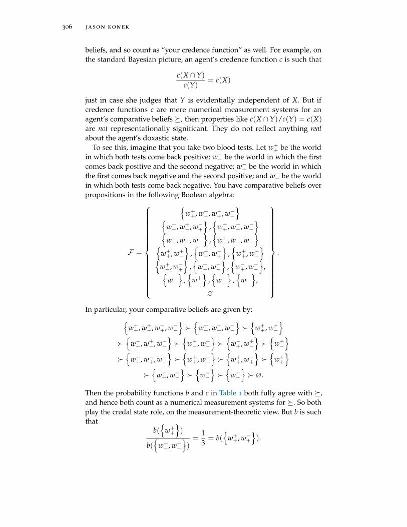
306 jason konek
beliefs, and so count as “your credence function” as well. For example, onthe standard Bayesian picture, an agent’s credence function c is such that
c(X ∩Y)c(Y)
= c(X)
just in case she judges that Y is evidentially independent of X. But ifcredence functions c are mere numerical measurement systems for anagent’s comparative beliefs , then properties like c(X ∩Y)/c(Y) = c(X)
are not representationally significant. They do not reflect anything realabout the agent’s doxastic state.
To see this, imagine that you take two blood tests. Let w++ be the world
in which both tests come back positive; w+− be the world in which the first
comes back positive and the second negative; w−+ be the world in whichthe first comes back negative and the second positive; and w−− be the worldin which both tests come back negative. You have comparative beliefs overpropositions in the following Boolean algebra:
F =
w++, w+
−, w−+, w−−
w++, w+
−, w−+
,
w++, w+
−, w−−
w++, w−+, w−−
,
w+−, w−+, w−−
w++, w+
−
,
w++, w−+
,
w++, w−−
w+−, w−+
,
w+−, w−−
,
w−+, w−−
,w++
,
w+−
,
w−+
,
w−−
,
∅
.
In particular, your comparative beliefs are given by:w++, w+
−, w−+, w−−
w++, w−+, w−−
w++, w+
−
w−+, w+−, w−−
w+−, w−−
w−+, w+−
w+−
w++, w−+, w−−
w++, w−−
w++, w−+
w++
w−+, w−−
w−−
w−+ ∅.
Then the probability functions b and c in Table 1 both fully agree with ,and hence both count as a numerical measurement systems for . So bothplay the credal state role, on the measurement-theoretic view. But b is suchthat
b(
w++
)
b(
w++, w+
−
)=
13= b(
w++, w−+
).

comparative probabilities 307
w++ w+
− w−+ w−−
b 1136
2236
136
236
c 2064
3364
464
764
Table 1: Probability functions b and c on F . Both fully agree with .
Given that b is your credence function, the standard interpretation says:you think that the result of the first test provides no evidence one way orthe other about the result of the second test. On the other hand, c is suchthat
c(
w++
)
c(
w++, w+
−
)=
2053
>2464
= c(
w++, w−+
).
Given that c is your credence function, the standard interpretation says:you judge that a positive outcome on the second test supports or confirmsa positive outcome on the first test. Finding out that the second test ispositive increases your credence that the first test is positive too.
What is going on here? Answer: the “standard interpretation” readsmore information into one’s credence function than is actually encodedin that credence function. On the measurement-theoretic view, credencefunctions are nothing more than numerical measurement systems thatencode the ordering determined by your comparative beliefs. (They aremere “ordinal scale” measurement systems, not “ratio scale” measurementsystems.) But there is more to making judgments of evidential relevanceand irrelevance than having a particular constellation of comparativebeliefs. Agents who only have comparative beliefs simply are not opinion-ated enough to count as having opinions about evidential relevance andirrelevance. So credence functions do not reflect any such opinions.
Interpreting imprecise credal states requires care too. Suppose, for ex-ample, that you have opinions about the propositions in the Booleanalgebra
F ∗ = Ω, X,¬X,∅ .
Consider the precise and imprecise credal states on F ∗ given by theprobability function b in Table 2 and the set of probability functions C:
Ω X ¬X ∅
b 1 0.7 0.3 0
Table 2: Probability function b on F ∗
C =
c | c(Ω) > c(X) > c(¬X) > c(∅)
.

308 jason konek
On the standard interpretation, b and C represent different doxastic states.An agent with credence function b is precisely 70% confident that X is true.An agent with imprecise credal state C, in contrast, is at least 50% confidentthat X is true, but nothing stronger. On the standard interpretation, theseare not idle differences. These differences in doxastic states are reflected inone’s evaluative attitudes. For example, an agent with credence function bwill have precisely the same fair buying and selling price for a unit gambleG on X, viz., 0.7. Paying any price up to £0.7 for G is a good deal in herview. Selling G for any price over £0.7 is a good deal. But an agent withimprecise credal state C will have different buying and selling prices for G.Paying any price up to £0.5 for G is a good deal, in her view. But selling Gis only a determinately good deal if the buyer is willing to pay more than£1.
On the measurement-theoretic view, however, b and C represent exactlythe same doxastic state. They both fully agree with the following comparativebelief relation :
Ω X ¬X ∅.
They are both order-preserving mappings from F ∗ into the reals thatpreserve exactly the same structure. In this case, there is simply no substantivedifference between being 70% confident, or 89.637% confident, or at least50% confident that X is true. Only the comparative beliefs that b andC encode are psychologically real. Everything else is a “mere artefact”of one’s preferred numerical measurement system. Both b and C, andany other credal state that fully agrees with , plays exactly the sametheoretical role: they represent the comparative beliefs captured by inan elegant, easy-to-use, numerical fashion—nothing more, nothing less.
5.2 Unary and Pluralist Variants
We have focussed thus far on a particular unary variant of the measurement-theoretic view. On this view, credence functions are mere numerical mea-sures of one’s comparative beliefs. Having credences is nothing over andabove having numerically representable comparative beliefs. You might beattracted to this view if, for example, you think that we can explain andrationalise everything important about choice and inference by appealingexclusively to comparative belief—no additional modes or types of dox-astic judgment necessary. In that case, you might say: to the extent thatwe are willing to talk about prima facie distinct types of opinion—degreesof belief, full or categorical belief, etc.—they ought to ultimately reduceto comparative beliefs. Reducing those other types of opinion away willallow us to provide the simplest and most unified possible explanationsof the relevant data regarding choice and inference.

comparative probabilities 309
But there is also a pluralist variant of the measurement-theoretic view,which you might find attractive if you are less optimistic about the explana-tory power of comparative belief. On the pluralist version, agents havea genuine plurality of doxastic attitudes, not simply comparative beliefs.In addition to comparative beliefs, agents also have: (i) opinions aboutthe evidential dependence or independence of one hypothesis on another; (ii)opinions about the causal dependence or independence of one variable onanother; (iii) full or categorical beliefs; they may even (iv) explicitly estimatethe values of all sorts of different variables, including the frequency oftruths in a set of propositions, and the truth-values of individual proposi-tions. Estimating, in this sense, is a matter of making a sui generis doxasticjudgment—a type of judgment that may bear interesting relations to othertypes of judgments (normative relations, causal relations, etc.), but is notreducible to them. Estimating the truth-value of a proposition, in thissense, is what Jeffrey (2002) calls having an exact judgmental probability forthe truth of that proposition.
On the pluralist measurement-theoretic view, your credence functionis a mere numerical measurement system, but not a measure specificallyof your comparative belief relation. Rather, on the pluralist view, you have agenuine plurality of comparative and qualitative doxastic attitudes, andyour credence function is a measure of that entire system of attitudes.
Consider once again our blood test example. You have the followingcomparative beliefs:
w++, w+
−, w−+, w−−
w++, w+
−, w−−
w++, w−+, w+
−
w++, w+
−
w−+, w+−, w−−
w+−, w−−
w−+, w+−
w+−
w++, w−+, w−−
w++, w−−
w++, w−+
w++
w−+, w−−
w−−
w−+ ∅.
But now imagine that you have a wide range of comparative and quali-tative opinions, not just comparative beliefs. You think, for example, thatwhen you find out the result of the first test (positive or negative), this pro-vides no evidence one way or the other about the result of the second test.(Perhaps the tests probe two different, unrelated conditions.) That is, youjudge w+
+, w+− and w−+, w−− to be evidentially independent of w+
+, w−+and w+
−, w−−, and vice versa.In addition, you have certain full beliefs or categorical beliefs. Let’s suppose
that you believe that the first test will come back positive. (It probes for acondition that you quite clearly have.) That is, you fully believe w+
+, w+−.
And you believe all of the logical consequences of this proposition. Butyou have no further full or categorical beliefs.

310 jason konek
Finally, you judge 1/3 to be the best estimate of the truth-value of theproposition that the second test will come back positive. (Recall, a proposi-tion’s truth-value is 1 if it is true and 0 if it is false.) In Jeffrey’s parlance,you have a judgmental probability of 1/3 for the proposition w+
+, w−+.So you have a genuine plurality of doxastic attitudes: you have com-
parative beliefs; you make evidential independence judgments; you havefull or categorical beliefs; you also estimate the truth-values of certainpropositions (you have exact judgmental probabilities). On the pluralistmeasurement-theoretic view, your credence function is a measure of thisentire system of attitudes.
To make this more precise, let’s model your doxastic attitudes using arelational structure:
A =⟨F ,, I ,B, E1/3
⟩.
A comprises your Boolean algebra F of subsets of Ω = w++, w+
−, w−+, w−−,together with a comparative belief relation on F , an independence relationI , a (unary) belief relation B, and a (unary) estimation relation E1/3.I models your evidential independence judgments. It will be convenient
to think of I as a 3-place relation on F :
I(X, Y, X ∩Y)iff
you judge X to be evidentially independent of Y.
Since you judge w++, w+
− and w−+, w−− to be independent of w++, w−+
and w+−, w−−, and vice versa, we have:
I(
w++, w+
−
,
w++, w−+
,
w++
),
I(
w−+, w−−
,
w++, w−+
,
w−+),
I(
w++, w+
−
,
w+−, w−−
,
w+−
),
I(
w−+, w−−
,
w+−, w−−
,
w−−).
We also have I(Y, X, X∩Y) for each of these four independence judgmentsI(X, Y, X ∩Y).
Likewise, B models your full or categorical beliefs:
B(X) iff you believe X.

comparative probabilities 311
Since you believe w++, w+
− and all of its logical consequences, we have:
B(
w++, w+
−, w−+, w−−),
B(
w++, w+
−, w−+),
B(
w++, w+
−, w−−),
B(
w++, w+
−
).
Finally, E1/3 models your explicit estimates of truth-values:
Ex(X)
iffyou judge x to be the best estimate of the truth-value of X.
Since you judge 1/3 to be the best estimate of the truth-value of w++, w−+,
we have:
E1/3
(w++, w−+
).
On the pluralist view, your credence function is a measure of your entiresystem of attitudes:
A =⟨F ,, I ,B, E1/3
⟩.
It is a homomorphism—a structure-preserving mapping—that takes Ainto some numerical structure A∗.
A∗ =⟨
R,∗, I∗,B∗, E∗1/3
⟩.
That is, your credence function c maps F into R in a way that preservesA’s structure, so that:13
X Y ⇔ c(X) ∗ c(Y),
I(X, Y, X ∩Y) ⇔ I∗(c(X), c(Y), c(X ∩Y)),
B(X) ⇔ B∗(c(X)),
E1/3(X) ⇔ E∗1/3(c(X)).
Which numerical structure c takes A into, on the measurement-theoreticview, is either a matter of convention or a matter to be decided on prac-tical grounds. For illustrative purposes, let’s choose a familiar numericalstructure. Let ∗ by the “greater than or equal to” relation, ≥. Let I∗ bethe standard probabilistic independence relation:
I∗(c(X), c(Y), c(X ∩Y)) iff c(X)c(Y) = c(X ∩Y).
13 We could swap full agreement for almost, or partial, or strong agreement here. Weakernotions of agreement would provide us with weaker notions of structure-preservation.

312 jason konek
Let B∗ be a Lockean belief relation, so that believed propositions X havereal-valued proxies c(X) that are greater than (or equal to) some thresholdτ (for concreteness let τ = 5/6):
B∗(c(X)) iff c(X) ≥ τ.
Finally, let E∗1/3 be:E∗1/3(c(X) iff c(X) = 1/3.
This ensures that for any structure-preserving measurement system, c, youexplicitly judge 1/3 to be the best estimate of X’s truth-value just in casec(X) = 1/3.
The important observation to make is this: the pluralist view carves outa bigger job for credence functions to do than the reductive view. Credencefunctions must do more than preserve the order induced on F by yourcomparative belief relation. They must also preserve the structure inducedby your various other doxastic attitudes: your evidential independencejudgments, full or categorical beliefs, and so on. So a function c : F → R
may well do the work required to count as “your credence function” onthe unary view, but yet fall short of that mark on the pluralist view.
Consider, for example, the function b : F → R:
b(
w++, w+
−, w−+, w−−) = 1, b(
w++, w−+, w−−
) = 31/64,
b(
w++, w+
−, w−−) = 60/64, b(
w++, w−−
) = 27/64,
b(
w++, w−+, w+
−
) = 57/64, b(
w++, w−+
) = 24/64,
b(
w++, w+
−
) = 53/64, b(
w++
) = 20/64,
b(
w−+, w+−, w−−
) = 44/64, b(
w−+, w−−
) = 11/64,
b(
w+−, w−−
) = 40/64, b(
w−−) = 7/64,
b(
w−+, w+−
) = 37/64, b(
w−+) = 4/64,
b(
w+−
) = 33/64, b(∅) = 0.
It is easy to verify that b fully agrees with , i.e.,
X Y ⇔ b(X) ≥ b(Y).
So b is a real-valued measure of your comparative belief relation . Hence,it counts as a credence function on the unary measurement-theoretic view.It preserves the structure on F induced by your comparative beliefs—theonly type of doxastic attitude that the unary view countenances. But it doesnot play the theoretical role required to count as a credence function onthe pluralist measurement-theoretic view. To do that, it must also preserve

comparative probabilities 313
the structure on F induced by your various other doxastic attitudes: yourindependence judgments, full or categorical beliefs, and so on. But b fallsshort of that mark.
For example, you think that the outcome of the first test provides noevidence about the outcome of the second. But b does not treat w+
+, w+−
and w++, w−+, for example, as independent, in the way specified by I∗:
b(
w++, w+
−
)b(
w++, w−+
)=
5364· 24
64=
159512
6= 160512
=2064
= b(
w++
).
Similarly, you believe that the first test will come back positive. That is,you fully believe w+
+, w+−. But b does not treat w+
+, w+− as believed, in
the way specified by the Lockean belief relation B∗. It maps w++, w+
− toa real-valued proxy b(w+
+, w+−) = 53/64 ≈ 0.828 below the threshold
τ = 5/6 ≈ 0.833 required for full or categorical belief.Finally, you judge 1/3 to be the best estimate of the truth-value of
the proposition that the second test will come back positive. You have ajudgmental probability of 1/3 for the proposition w+
+, w−+. But b failsto map w+
+, w−+ to the real-valued proxy set aside by E∗1/3 for suchpropositions, viz., 1/3. Instead, b(w+
+, w−+) = 24/64 = 0.375.The upshot: while b preserves the structure on F induced by your com-
parative beliefs, it fails to preserve the additional structure induced by yourvarious other doxastic attitudes: your evidential independence judgments,full or categorical beliefs, and so on. So while b does count as one of your(infinitely many) credence functions on the unary measurement-theoreticview, it does not count as one on the pluralist measurement-theoretic view.
In contrast, the function c : F → R of Figure 6 counts as “your credencefunction” on both the unary and pluralist views. (The interested readermay verify this for herself.)
To recap: the measurement-theoretic view stakes out a particular posi-tion on the theoretical role R that a function c (or set of functions C) mustplay in order to count as “your credal state.” It says that c (or C) mustfully agree (or almost agree, or partially agree, or strongly agree) withyour comparative and qualitative opinions—comparative beliefs, eviden-tial independence judgments, full or categorical beliefs, etc.—in the wayrequired to count as a numerical measure of that entire system of attitudes.The better c (or C) plays this role R, the more eligible it is as a credal statecandidate. On the unary measurement-theoretic view, the fundamentaltype of doxastic attitude is comparative belief. So credal states are numericalmeasures of comparative beliefs. On the pluralist measurement-theoreticview, you have a genuine plurality of doxastic attitudes. So credal statesare numerical measures of a more highly structured system of attitudes.

314 jason konek
c(
w++, w+
−, w−+, w−−) = 1, c(
w++, w−+, w−−
) =
1436
,
c(
w++, w+
−, w−−) =
3536
, c(
w++, w−−
) =
1336
,
c(
w++, w−+, w+
−
) =
3436
, c(
w++, w−+
) =
1236
,
c(
w++, w+
−
) =
3336
, c(
w++
) =
1136
,
c(
w−+, w+−, w−−
) =
2536
, c(
w−+, w−−) =
336
,
c(
w+−, w−−
) =
2436
, c(
w−−) =
236
,
c(
w−+, w+−
) =
2336
, c(
w−+) =
136
,
c(
w+−
) =
2236
, c(∅) = 0.
Figure 6: Credence function c
To streamline our discussion, we will focus on the the unary variant ofthe measurement-theoretic view going forward.
5.3 The Characterisation and Normative Questions
How does the unary measurement-theoretic account answer the charac-terisation question? When exactly is there a function c (or set C) that fullyagrees (or almost agrees, or partially agrees, or strongly agrees) with yourcomparative belief relation in the way required to count as a numericalmeasure of ?
We explored a partial answer to this question earlier. Scott (1964) provesthat there is a probability function that fully agrees with your comparativebelief relation just in case satisfies Non-Triviality, Non-Negativity,Totality, and Isovalence. Rios Insua (1992) and Alon and Lehrer (2014)prove that there is a set of probability functions that fully agrees with just in case satisfies Reflexivity, Non-negativity, Non-triviality, and theGeneralised Finite-Cancellation axiom. Kraft et al. (1959) proves that thereis a probability function that almost agrees with just in case it satisfiesAlmost-Cancellation. Adams (1965) and Fishburn (1969) prove that thereis a probability function that partially agrees with just in case it satisfiesPartial-Cancellation. Finally, in proving the Generalised Scott Theorem, weidentified sufficient conditions for the existence of a probability functionthat strongly agrees with : Non-Triviality, Non-Negativity, and Isovalence.

comparative probabilities 315
Pinning down necessary and sufficient conditions for strong representabil-ity is an open problem.
These representation theorems tell us what it takes to count as havingprobabilistically coherent credences, on the measurement-theoretic view. Butthey do not answer the more general characterisation question: when isyour comparative belief relation sufficiently well-behaved for you to countas having credences full stop, coherent or not?
Krantz et al. (1971) provide an answer. They show that a comparativebelief relation fully agrees with a real-valued function c if and only if is a weak order, i.e., satisfies Transitivity and Totality (Krantz et al.,1971, p. 15, Theorem 1). So if a real-valued function c counts as a structure-preserving numerical measure of just in case c fully agrees with ,and if precise credence functions just are structure-preserving numericalmeasures of , then we now know exactly when you count as havingprecise credences full stop. You count as having precise credences just incase satisfies Transitivity and Totality.
Weaker notions of agreement set weaker standards for “structure preser-vation.” They thereby make it easier for a real-valued function (or setof functions) to count as a structure-preserving numerical measurementsystem for . In turn, your comparative beliefs need not satisfy suchstrict constraints for you to count as having credences. For example, everycomparative belief relation almost agrees with a real-valued function c.So if all that is required for structure-preservation is almost-agreement,then nothing whatsoever is required of for you to count as having cre-dences. Any comparative belief relation will do. More interestingly, strongly agrees with a real-valued function c if and only if satisfies weaktransitivity (see the appendix for proof).14
Weak Transitivity. If X Y1 . . . Yn Z, then X 6≺ Z.
So if structure-preservation requires strong-agreement and nothing more,then you count as having precise credences just in case satisfies WeakTransitivity.
What then of Meacham and Weisberg’s concern? They claim that theaxioms of typical representation theorems for comparative belief are sodemanding that only perfectly rational agents could possibly satisfy them.So even if those axioms do encode sufficient conditions for having cre-dences, they are more or less irrelevant for irrational agents like us. Theyleave entirely open whether our comparative beliefs are ever well-behavedenough for us to count as having credences.
But your comparative beliefs need not satisfy the axioms of Scott’sTheorem (or the Almost-Cancellation axiom, or the Partial-Cancellationaxiom, etc.) for you to count as having credences. Such axioms encode
14 The proof strategy for this theorem is due to Catrin Campbell-Moore.

316 jason konek
necessary and sufficient conditions for having probabilistic credences. Prob-abilistic credence functions, however, are not the only credence functionsin town. Your comparative beliefs only need to satisfy weaker constraints,such as Weak Transitivity, to count as having credences tout court. WeakTransitivity is not nearly as demanding as Scott’s axiom.
It is also worth nothing that even though Scott’s axiom and the likeseem complicated, it is not obvious that they are excessively difficult foragents like us to satisfy. It may be computationally intensive to run adiagnostic program which continually checks your comparative beliefsfor violations of Scott’s axiom. And if we had to run such a programto reliably satisfy Scott’s axiom, then you might well expect that limitedagents like us typically violate it. But no such program is necessary. Natureis replete with cheap solutions to seemingly computationally intensiveproblems. This is one main lesson of the embodied cognition movementin cognitive science.15 Agents like us might well use computationallycheap strategies, rather than demanding diagnostic programs, in order tominimise violations of Scott’s axiom and other coherence constraints.
Meacham and Weisberg also worry that the measurement-theoretic viewand its ilk count the wrong functions as eligible credal state candidates(Meacham & Weisberg, 2011, p. 5). On the (unary) measurement-theoreticview, any of the infinitely many numerical measurement systems for count as equally eligible credal state candidates. But some clearly are moreeligible than others. For example, suppose that Holmes has opinions aboutfinitely many propositions, e.g., about whether Moriarty is in London, etc.Then Holmes is struck on the head. The blow does not change Holmes’comparative beliefs. He is still more confident that Moriarty is in Londonthan Paris, and so on. But it does raise his confidence that Moriarty is inLondon. Then clearly something has changed about which functions arethe most eligible candidates for counting as Holmes’ credence function.But on the measurement-theoretic view, nothing at all has changed.
One of two things is going on here. Option 1: the objection tacitlypresupposes that the measurement-theoretic view simply misidentifies thetheoretical role R that a function c (or set C) must play in order to countas “your credal state.” That is a meaty, substantive debate, and we willnot explore it any further. Option 2: the objection tacitly presupposes thatHolmes makes explicit judgments about the best estimates of truth-values,or something of the sort. But that assumes pluralism. And the pluralist
15 Consider, for example, the “outfielder’s problem” (Clark, 2015, p. 12). It might seemmiraculous that baseball players manage to catch fly balls if doing so involves: (i) estimatingthe position of a ball at various time points; (ii) using this information to estimate theball’s trajectory; (iii) calculating where the ball will land on the basis of its trajectory. Thisis computationally intensive! Luckily, there is a computationally cheap solution. You canjust move your body in a way that keeps the ball centred in your visual field. This strategyuses the agent’s body to reduce computational demand.

comparative probabilities 317
measurement-theoretic view simply does not say that any of the infinitelymany numerical measurement systems of Holmes’ comparative beliefs areequally eligible candidates for counting as Holmes’ credence function.
So much for the characterisation question. How does the unarymeasurement-theoretic account answer the normative question? Whyshould we expect rational agents to have probabilistically coherent credences?
How we answer the normative question depends on what we say aboutstructure preservation. If we say, for example, that c must fully agree with to count as a structure-preserving numerical measure of , and in turncount as “your credal state,” then the following argument answers thenormative question.
1. Coherence Constraints. Any rational agent’s comparative belief rela-tion satisfies Non-Triviality, Non-negativity, Totality, and Isova-lence.
2. Theory of Credence. A real-valued function c (or set C) counts as“your credal state” just in case it is a structure-preserving numericalmeasure of , i.e., just in case it plays the “structure-preservationrole” R. And c preserves the structure of just in case c fully agreeswith .
3. Scott’s Theorem. Relation satisfies Non-Triviality, Non-negativity,Totality, and Isovalence if and only if fully agrees with someprobability function c.
4. Bridge Theorem. If satisfies Non-Triviality, Non-negativity, Totality,and Isovalence, then there is some probability function c that playsrole R well enough to count as “your credal state.” (From 2 and 3)
C. Probabilism. Any rational agent has probabilistic credences. (From 1and 4)
Now, you might quibble with premise 1. You might doubt whether Totality,for example, encodes a genuine constraint of rationality. In that case,we might weaken our putative coherence constraints by adopting lessdemanding standards for structure preservation. For example, if we saythat structure preservation requires only strong agreement with , ratherthan full agreement, then we can offer the following argument.
1∗. Coherence Constraints. Any rational agent’s comparative belief rela-tion satisfies Non-Triviality, Non-negativity, and Isovalence.
2∗. Theory of Credence. A real-valued function c (or set C) counts as“your credal state” just in case it is a structure-preserving numericalmeasure of , i.e., just in case it plays the “structure-preservation

318 jason konek
role” R. And c preserves the structure of just in case c stronglyagrees with .
3∗. Corollary of GST. If satisfies Non-Triviality, Non-negativity, andIsovalence, then strongly agrees with some probability function c.
4∗. Bridge Theorem. If satisfies Non-Triviality, Non-negativity, andIsovalence, then there is some probability function c that plays roleR well enough to count as “your credal state.” (From 2∗ and 3∗)
C∗. Probabilism. Any rational agent has probabilistic credences. (From 1∗
and 4∗)
Each type of agreement (full, strong, almost, partial) yields a differentvariant of this argument. Whether you find any of them compelling willdepend on (i) which putative coherence constraints you find plausibleor implausible (premise 1), and (ii) what type of agreement is requiredfor credence functions to play any auxiliary theoretical roles you deemimportant (premise 2).
At this point, you might be a bit suspicious. Doesn’t this argument trivi-alise probabilism? True enough, you might say, the probability functionsoutputted by Scott’s theorem are fit to play the “credal state role” R onmeasurement-theoretic view. But that is because we reverse engineeredR so that Scott’s theorem outputs exactly the right sorts of functions toplay R! We stipulatively defined R to be the role of preserving the structureof . Then we stipulatively defined structure-preservation to be a matterof fully agreeing with . But given these stipulative definitions, it followstrivially that the probability functions outputted by Scott’s theorem playR well enough to count as “your credal state.” Probabilism seems less likea substantive normative thesis, then, and more like a trivial consequenceof stipulative definitions.
This suspicion is doubly off the mark. Firstly, the measurement-theoreticaccount of credence puts forward a substantive claim about the principaltheoretical role of credence functions c (and imprecise credal states C). It ismotivated by the thought that our opinions are qualitative. At bottom, wehave opinions like: comparative beliefs, full beliefs, etc. And the best wayto understand the numbers that we use to describe these qualitative atti-tudes is in exactly the same way that we understand the numbers that weuse to describe length, mass, volume, etc., viz., as numerical measurementsystems. Whether this is right or wrong, it is surely no stipulative definition.Secondly, as we have already emphasised, representability by a probabilityfunction is strictly stronger than representability by a real-valued function.Establishing that the stronger axioms (e.g., Scott’s axioms) encode genuineconstraints of rationality, rather than merely the weaker axioms (e.g., Tran-sitivity and Totality) is non-trivial. As a result, establishing probabilism is
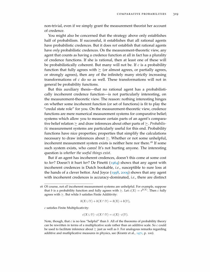
comparative probabilities 319
non-trivial, even if we simply grant the measurement theorist her accountof credence.
You might also be concerned that the strategy above only establisheshalf of probabilism. If successful, it establishes that all rational agentshave probabilistic credences. But it does not establish that rational agentshave only probabilistic credences. On the measurement-theoretic view, anyagent that counts as having a credence function at all in fact has a pluralityof credence functions. If she is rational, then at least one of these willbe probabilistically coherent. But many will not be. If c is a probabilityfunction that fully agrees with (or almost agrees, or partially agrees,or strongly agrees), then any of the infinitely many strictly increasingtransformations of c do so as well. These transformations will not ingeneral be probability functions.
But this auxiliary thesis—that no rational agent has a probabilisti-cally incoherent credence function—is not particularly interesting, onthe measurement-theoretic view. The reason: nothing interesting hingeson whether some incoherent function (or set of functions) is fit to play the“credal state role” for you. On the measurement-theoretic view, credencefunctions are mere numerical measurement systems for comparative belief;systems which allow you to measure certain parts of an agent’s compara-tive belief relation and draw inferences about other parts of . Probabilis-tic measurement systems are particularly useful for this end. Probabilityfunctions have nice properties; properties that simplify the calculationsnecessary to draw inferences about . Whether or not some unhelpful,incoherent measurement system exists is neither here nor there.16 If somesuch system exists, who cares! It’s not hurting anyone. The interestingquestion is whether the useful things exist.
But if an agent has incoherent credences, doesn’t this come at some costto her? Doesn’t it hurt her? De Finetti (1964) shows that any agent withincoherent credences is Dutch bookable, i.e., susceptible to sure loss atthe hands of a clever bettor. And Joyce (1998, 2009) shows that any agentwith incoherent credences is accuracy-dominated, i.e., there are distinct
16 Of course, not all incoherent measurement systems are unhelpful. For example, supposethat b is a probability function and fully agrees with . Let c(X) = eb(X). Then c fullyagrees with . But while b satisfies Finite Additivity:
b(X ∪Y) + b(X ∩Y) = b(X) + b(Y),
c satisfies Finite Multiplicativity:
c(X ∪Y) · c(X ∩Y) = c(X) · c(Y).
Note, though, that c is no less “helpful” than b. All of the theorems of probability theorycan be rewritten in terms of a multiplicative scale rather than an additive scale. So c couldbe used to facilitate inference about just as well as b. For analogous remarks regardingadditive and mutliplicative measures in physics, see (Krantz et al., 1971, p. 100).

320 jason konek
(coherent) credences that are guaranteed to be closer to the truth thanhers. Aren’t these costs—pragmatic and epistemic—that any agent withincoherent credences must pay?
No. Not on the measurement-theoretic view. De Finetti assumes thatif c counts as your credence function, then c(X) is both your fair buyingand selling price for a unit gamble on X. But this is simply not so on themeasurement-theoretic view. Credence functions represent your compara-tive beliefs in an elegant, easy-to-use, numerical fashion—nothing more,nothing less. It is simply not the job of a credence function to capture yourfair buying (or selling) prices. We cannot read your fair buying and sellingprices off of c in any straightforward fashion. Indeed, to infer anythingabout your betting behaviour from c, we need decision-theoretic normsthat specify how rational comparative beliefs and preferences hang together.For example, following (Savage, 1954, Section 3.2), we might suggest thefollowing.
Coherence. If X Y, then you ought to prefer to stake goodoutcomes on X than Y. More carefully, if you strictly preferoutcome o to o∗, and X Y, then you ought to strictly preferA to B:
A = [o if X, o∗ if ¬X] ,
B = [o if Y, o∗ if ¬Y] .
Moreover, you ought to be willing to sacrifice some smallamount ε to exchange A for B.
If you satisfy Coherence, and c fully agrees with , then we can use c toinfer something about your betting behaviour. For example, if c(X) = 0.7and c(Y) = 0.6, then we can infer that you prefer to let £1 ride on X thanon Y, and would even be willing to pay some small amount to exchangethe first gamble for the second. But we cannot infer that your fair buying(selling) price for X is £0.7, or that your fair buying (selling) price for Y is£0.6.
Without this crucial assumption—that credences encode fair buy-ing/selling prices—we cannot provide a de Finetti-style Dutch bookargument to show that no rational agent has incoherent credences. Havingan incoherent credence function does not mean that you have inco-herent fair buying/selling prices, and hence does not mean that yourbuying/selling prices render you Dutch-bookable.
In a similar fashion, Joyce assumes that if c counts as your credencefunction, then c(X) is your best estimate of X’s truth-value. Moreover, theaccuracy of these estimates is what makes your doxastic state better orworse from the epistemic perspective. (Accuracy is the principal source ofepistemic value, anyway.) But again, this is not so on the measurement-theoretic view. Credence functions are mere numerical measures of com-

comparative probabilities 321
parative belief relations. It is simply not the job of a credence function tocapture your best estimates of truth values, on the measurement-theoreticview. The upshot: having an incoherent credence function does not meanthat you in any sense have incoherent truth-value estimates; so it does notmean having accuracy-dominated truth-value estimates; so it does not meanhaving a doxastic state that is epistemic-value-dominated.
Finally, one might level a criticism similar to Meacham and Weisberg’s(2011, pp. 19–20) criticism of Lyle Zynda. Zynda is a proponent of theunary measurement-theoretic account (Zynda, 2000, pp. 66–68).17 OnZynda’s view, there are comparative beliefs—agents are more confidentin some propositions than others—but there are no additional modes ortypes of doxastic judgment. To the extent that we countenance talk of fullybelieving a proposition, or believing something much more strongly thansomething else, this better ultimately reduce to talk about comparativebeliefs.
Meacham and Weisberg object that comparative beliefs lack the structurerequired to explain everything about choice and inference that we wouldlike to explain. So even if the measurement theorist provides some reasonto expect rational agents to have probabilistic credences, the backgroundpicture of the basic stock of doxastic attitudes available to such agents istoo impoverished for their arguments to cut much ice.
For example, if we buy the unary measurement-theoretic account, thenthe well-known problem of interpersonal utility comparisons rears itshead as a problem of interpersonal credal comparisons. Just as it makesno sense to say that Ashan desires chocolate ice cream more stronglythan Bilal does, on the measurement-theoretic account (since there isno common scale one which their preferences are measured), similarlyit makes no sense to say that Ashan is more confident that it will rainthan Bilal is. But, at least in certain cases, it seems that we need suchfacts to explain choice behaviour. Why did Ashan grab his umbrella butBilal did not? One possible explanation: both are more confident thannot that it will rain, but Ashan is more confident than Bilal. On the theunary measurement-theoretic account, such explanations are unavailable,Meacham and Weisberg argue. More generally:
the extra-ordinal structure contained in the standard Bayesianpicture of degrees of belief is not idle. Magnitudes encode im-portant features of our degrees of belief, and if we abandon thisstructure, degrees of belief lose much of their utility. (Meacham& Weisberg, 2011, p. 20)
17 Like Maher, Zynda subscribes to the thesis of the primacy of practical reason (cf., Zynda2000, p. 55). Credence functions are numerical measures of comparative beliefs. Butpreferences are the real thing. Comparative beliefs reduce to preferences.

322 jason konek
You might not think that there is much to this line of criticism. Forexample, Ashan might think that rain is just as likely as picking a blackball at random from an urn containing 99 black balls and 1 white ball. Bilal,in contrast, might think that rain is just as likely as picking a black ball atrandom from an urn containing 51 black balls and 49 white balls.18 Theseindividual comparative belief facts help to explain why Ashan grabbed hisumbrella but Bilal did not at least as well as the purported interpersonalfact that Ashan is more confident than Bilal. It is not obvious, then, thatthere is any genuine problem of interpersonal credal comparisons toresolve.
Even if you do think there is something to this line of criticism, notethat it is not an objection to the measurement-theoretic account of cre-dence per se. It is only an objection to the unary measurement-theoreticaccount. A pluralist faces no such problems. Of course, in answering thenormative question, a pluralist cannot simply appeal to Scott’s theorem.Scott’s theorem only shows that comparative belief relations with certainproperties are probabilistically representable. The pluralist must appealto a representation theorem that shows that a more comprehensive system ofdoxastic attitudes with certain properties is probabilistically representable.But there is no principled reason for thinking that such representationtheorems are not forthcoming.
6 evaluating the decision-theoretic view
On the decision-theoretic view, the principal theoretical role of an agent’scredal state is to encode her fair buying and selling prices. Recall, anagent’s fair buying price for a gamble G is the largest amount B(G) thatshe could pay for G without making herself worse off. She pays B(G),receives G, and is no worse than the status quo, in her own view. Her fairselling price for G is the smallest amount S(G) that someone else wouldhave to pay her in exchange for G to avoid being worse off. She receivesS(G), commits to shelling out G’s payoff, and is no worse than the statusquo, in her own view.
Gambles are measurable quantities G : Ω→ R. For simplicity, we willassume that |Ω| = n, and treat gambles as vectors in Rn. When we modela gamble as a vector
G = 〈g1, . . . , gn〉 ,
18 Both de Finetti (1931) and Koopman (1940a) use “partition axioms” to extract quantitativeinformation from belief relations in roughly this way. For a recent approach along theselines, see Elliott (2018). You might also model agents as having comparative estimationrelations, as explored in §2.3. Comparative estimation relations allow for a much richerand explanatorily powerful set of doxastic attitudes than comparative belief relations.

comparative probabilities 323
we do so by specifying the net effect gi that the gamble has on our agent’slevel of total wealth in world wi. For example, suppose you let £100 rideon red at the roulette table. Let w1, . . . , wi be the worlds in which the balllands on red (you net £100), and wi+1, . . . , wn be the worlds in which itdoes not (you net −£100). Then we model your gamble as follows:
G =
⟨100, . . . , 100︸ ︷︷ ︸
i times
,−100, . . . ,−100︸ ︷︷ ︸(n-i) times
⟩.
For any proposition X ∈ F , we model a unit gamble on X by thecharacteristic vector x = 〈x1, . . . , xn〉 of X, i.e., the vector with xi = 1if wi ∈ X and xi = 0 if wi 6∈ X. And for any a ∈ R, we model the“constant gamble” that pays out £a in every world by the constant vectora = 〈a, . . . , a〉.
Following Walley (1991), we can specify an agent’s fair buying andselling prices using sets of almost-desirable gambles. Say that a gamble Gis almost desirable for an agent iff she weakly prefers G to 〈0, . . . , 0〉, i.e.,the status quo. Let D ⊆ Rn be the set of gambles that she finds almostdesirable.
Now we can specify her fair buying and selling price for G (B(G) andS(G), respectively) in terms of D. Let
B(G) = sup
a | G − a ∈ D
.
Taking the gamble G − a is equivalent to paying £a for G. So B(G) is thelargest amount that she could pay for G while leaving herself in a positionthat she weakly prefers to the status quo, i.e., her fair buying price for G.Likewise, let
S(G) = inf
a | a− G ∈ D
.
Taking the gamble a− G is equivalent to receiving £a and shelling outG’s payoff. So S(G) is the smallest amount that someone else would haveto pay her in exchange for G while leaving herself in a position that sheweakly prefers to the status quo, i.e., her fair selling price for G.
Talk of both fair buying and fair selling prices is actually a bit redundant.Note that
−B(−G) = − supa | −G − a ∈ D
= inf
−a | −G − a ∈ D
= inf
a | −G + a ∈ D
= S(G).
Taking −G from someone (they shell out −G’s payoff to you) is nothingmore than you offering G to them (you shell out G’s payoff to them). And

324 jason konek
paying a negative amount to someone for some good is really nothing morethan them paying you a positive amount (and vice versa: taking a negativeamount is nothing more than you paying a positive amount). The smallerthe positive amount that they pay you, the bigger the negative amountyou pay them. So the negative of the biggest amount that you would payto take −G, i.e., −B(−G), is just another way of describing the smallestamount that you would need to be paid to offer G.
We will just talk of your fair buying prices henceforth. But these reallycapture both your fair buying and selling prices.
Say that a set E of real-valued functions e : Rn → R encodes your fairbuying prices iff its lower envelope for G,
E [G] = inf
e(G) | e ∈ E
,
is equal to B(G) when B(G) is defined, and is undefined when it is not. Saythat a set of probability functions C encodes your fair buying prices just incase its corresponding set of expectation operators EC =
Ec | c ∈ C
does
so:EC [G] = inf
Ec[G] | c ∈ C
.
Finally, say that your fair buying prices are probabilistic iff some set ofprobability functions encodes them.
How does the decision-theoretic account answer the characterisationquestion? When exactly is there a real-valued function c (or a set of suchfunctions C) that encodes your fair buying and selling prices? Answer:always.
Say that a real-valued function e : Rn → R dominates your fair buyingprices iff e(G) ≥ B(G) whenever B(G) is defined. Let E∗ be the set ofreal-valued functions that dominate your fair buying prices, i.e.,
E∗ =
e | e(G) ≥ B(G) if B(G) is defined
.
Then E∗ encodes your fair buying prices, whatever they are. Hence E∗counts as “your credal state” according to the decision-theoretic view.
So there are no demanding constraints that an agent must satisfy inorder to have credences, on this view. Having credences is dead easy. Andclearly it is perfectly possible to have non-probabilistic credences.
So much for the characterisation question. How does the decision-theoretic account answer the normative question? Why should we expectrational agents to have probabilistic credences?
The story here is considerably more tricky. One might expect standardDutch book arguments to provide an answer. De Finetti (1964) shows thatfor a specific sort of agent—one whose fair buying prices are equal toher fair selling prices, i.e., B(G) = S(G)—having non-probabilistic fairbuying prices renders you Dutch bookable (susceptible to sure loss at

comparative probabilities 325
the hands of a clever bettor). One can see essentially the same result byconsidering (Walley, 1991, 3.3.3a). Walley shows that an agent’s fair buyingprices are not Dutch bookable (avoid sure loss) iff they are dominated bythe expectation operator of some probability function. And in the specialcase under consideration—fair buying prices equal fair selling prices—one’s fair buying prices are dominated in this way just in case they areprobabilistic, i.e., encoded by some set of probabilities C. The upshot: inthis special case—fair buying prices equal fair selling prices—an agent isnot Dutch bookable (avoids sure loss) iff there is some set of probabilities Cthat encodes her fair buying prices, and hence counts as “her credal state.”So if rationality requires avoiding sure loss, then we have good reason toexpect this very special kind of agent to have probabilistic credences.
You might hope, then, that such a Dutch book argument could showquite generally that rational agents have probabilistic credences. But yourhopes would be in vain. An agent avoids sure loss iff there is some setof probabilities C whose expectations for gambles uniformly dominateher fair buying prices for those gambles, i.e., Ec[G] ≥ B(G) for all c ∈ Cand all gambles G. When an agent’s fair buying and selling prices comeapart, this can happen even when there is no set of probabilities C∗ thatactually encodes her fair buying prices.19 Bottom line: non-Dutch-book-ability (avoiding sure loss) does not require having probabilistic credences.
Having probabilistic credences, in the decision-theoretic sense (i.e., someset of probabilities that encodes your fair buying prices), is equivalent tosomething stronger than non-Dutch-book-ability—what Walley calls “co-herence.” Your fair buying prices are coherent iff they satisfy the followingaxioms.
1. Accept Sure Gains. B(G) ≥ infG.
2. Homogeneity. B(λG) = λB(G) for λ ≥ 0.
3. Superlinearity. B(G + G∗) ≥ B(G) + B(G∗).
Axiom 1 forbids you from paying at most £1 for G when G is guaranteedto payoff either £2, £3, or £4, for example. It says that your maximumbuying price for G must be at least £2. Axiom 2 says that your fair buyingprice for a gamble G that is guaranteed to pay 2 (or 10, or 58.97) timesanother gamble G∗ should be 2 (or 10, or 58.97) times your fair buyingprice for G∗. Axiom 3 says that your fair buying price for a package of bets
19 Consider, for example, an agent whose fair buying price for any gamble G is infG − ε. Forany non-constant G, B(G) = infG − ε < supG − ε = − inf−G − ε < − inf−G + ε = S(G).But clearly B[G] < EC [G] for any set of probability functions C. So the lower envelope ofEC dominates her fair buying prices. Hence she avoids sure loss. But no such C encodes herfair buying prices.

326 jason konek
should be at least as great as the sum of your fair buying prices for eachof the bets in the package.
To reiterate: coherence is strictly stronger than avoiding sure loss. Walley(1991, Section 2.4) provides examples of fair buying prices that avoid sureloss (are not Dutch bookable), but nevertheless are not coherent. (Everycoherent set of fair buying prices, in contrast, avoids sure loss.) So Dutchbook or sure loss considerations do not give us good reason to think that,quite generally, rational agents have probabilistic credences.
All is not lost, though. Even if Dutch books arguments don’t do thetrick, another argument might. For example, in the spirit of Icard (2016)and Fishburn (1986, p. 338), we might propose constraints of rationalitygoverning how one’s comparative beliefs and preferences, or judgments ofalmost-desirability, ought to hang together. In particular, we might suggestthat the set D of gambles that an agent finds almost desirable (i.e., that sheweakly prefers to the status quo) ought to be exactly the set D of gamblesthat are almost desirable relative to her comparative belief relation .
Belief-Preference Coherence. D = D.
Recall, a gamble G is almost desirable relative to iff it is a non-negativelinear combination of components
(X1 −Y1), . . . , (Xn −Yn)
which are such that Xi Yi. G is a non-negative linear combination of(X1 −Y1), . . . , (Xn −Yn) just in case
G = ∑i
λi(Xi −Yi)
for some λ1, . . . , λn ≥ 0.The basic thought here is this. Xi − Yi is the gamble that pays out £1
if Xi is true and −£1 if Yi is true. You ought to weakly prefer this to thestatus quo iff you are at least as confident that Xi is true as Yi. Moreover,you ought to think that any package of such bets, even if their stakes arescaled up or down by a positive constant, is almost-desirable; you oughtto weakly prefer it to the status quo. And nothing more. Your comparativebeliefs give you no reason to determinately prefer any other gamble to thestatus quo.
Now suppose that rationality not only demands comparative beliefs andpreferences hang together as per Belief-Preference Coherence, but that italso demands that comparative beliefs on their own satisfy the GeneralisedFinite-Cancellation axiom.
Generalised Finite-Cancellation. If
X1 + . . . + Xn + A + . . . + A︸ ︷︷ ︸k times
= Y1 + . . . + Yn + B + . . . + B︸ ︷︷ ︸k times

comparative probabilities 327
and Xi Yi for all i ≤ n, then A B.
Perhaps pragmatic considerations other than Dutch book or sure lossconsiderations establish that rational comparative beliefs satisfy GFC.20
Or perhaps epistemic considerations establish this. Perhaps, for example,comparative beliefs that satisfy GFC epistemic-utility-dominate ones thatdo not, or something of the sort. For now, let’s just leave an IOU for thejustification of GFC.
Supposing that rational comparative beliefs satisfy GFC, we can nowprovide some reason to think that quite generally rational agents haveprobabilistic credences.
1. Coherence Constraints. Any rational agent’s comparative beliefs sat-isfy GFC. Moreover, her comparative beliefs and preferences, orjudgments of almost-desirability, jointly satisfy Belief-Preference Co-herence.
2. Theory of Credence. A set of real-valued functions C count as “yourcredal state” just in case they encode your fair buying prices.
3. IP-Representability Theorem. Relation satisfies GFC iff is IP-representable, i.e., fully agrees with some set of probability func-tions C.
4. Bridge Theorem. If is IP-representable and satisfies Belief-PreferenceCoherence, then the maximal set of probability functions C∗ thatfully agrees with also encodes your fair buying prices, and hencecounts as “your credal state.” (Premise 2, Appendix)
C. Probabilism. Any rational agent has probabilistic credences. (From 1,3, and 4)
Does this argument trivialise probabilism? Of course not. It relies on thedecision-theoretic account of credence—a substantive, highly non-trivialthesis. Moreover, even if we simply grant the decision-theoretic account ofcredence, it is no trivial consequence that rational agents have probabilisticcredences. Having credences is easy. You have credences whatever yourfair-buying prices are. But having probabilistic credences requires satisfyingsome demanding axioms (Belief-Preference Coherence, GFC). Establishingthat these axioms encode genuine constraints of rationality is non-trivial.As a result, establishing probabilism is non-trivial.
20 Icard (2016) shows that an agent who satisfies Belief-Preference Coherence avoids sure lossiff her comparative beliefs are strongly representable. Strong representability is weakerthan GFC. So we need something other than sure loss considerations to show that rationalcomparative beliefs satisfy GFC.
328 jason konek
You might be concerned that our little argument only establishes halfof probabilism. It shows that rational agents have probabilistic credences.But it does not show that rational agents have only probabilistic credences.Indeed, it cannot do so. We gave a recipe earlier for constructing a credalstate for any agent. Just take the set of real-valued functions that dominateher fair buying prices. This set will encode those prices, and so countas “her credal state,” on the decision-theoretic view. But it is not a set ofprobability functions.
But this converse thesis—viz., that for any rational agent, no set of real-valued functions with non-probabilistic members counts as “her credalstate”—is not theoretically interesting, on the decision-theoretic view. Thebenefits of having probabilistic credences (avoiding sure loss, coherence)accrue to any agent whose fair buying prices are encoded by some set ofprobabilities. Whether or not some non-probabilistic set encodes them aswell is neither here nor there. Nothing of theoretical import hangs on it.
Finally, you might once again complain that the decision-theoretic ac-count presupposes that rational agents only have comparative beliefs; noadditional modes or types of doxastic judgment. But this stock of basicdoxastic attitudes is too sparse. It is insufficient to explain everythingabout choice and inference that we would like to explain. So argumentsthat presuppose it are weak.
A similar response to the one in Section 5 will suffice. There is goodreason to think this criticism lacks punch. And even if you buy the criticism,it is not an objection to the decision-theoretic account of credence per se.It is only an objection to the unary variant of this account. A pluralistfaces no such problems. Of course, a pluralist must say more about howother types of doxastic attitudes—not just comparative beliefs—oughtto hang together with judgments of almost-desirability. In addition, shemust provide a more sophisticated IP-representability theorem and bridgetheorem. But these are not in-principle problems. They are requests tocash in an IOU.
What does the scorecard look like? Whether the decision-theoretic ac-count provides a compelling answer to the normative question dependsin part on whether those IOUs can be replaced by theorems. But there isno special reason to think this task cannot be done. In addition, epistemicutility theorists, e.g., Joyce (1998, 2009) and Pettigrew (2016), worry thatthis story provides an incomplete picture of our reasons to have proba-bilistic credences. A complete picture would provide a purely epistemicrationale for having imprecise credences.21 Nevertheless, some form of theargument presented here might help illuminate some of our reasons forhaving probabilistic credences.
21 Epistemic utility theorists get off the boat early by rejecting the decision-theoretic accountof credence.

comparative probabilities 329
7 evaluating the epistemic interpretivist view
On the epistemic interpretivist view, a function (or set of functions) countsas “your credal state” just in case it encodes truth-value estimates thatbest rationalise or make sense of your comparative beliefs, understood asirreducibly-doxastic attitudes.
More formally, a function c : F → R (or a set of such functions C)counts as “your credal state” iff its truth-value estimates best rationaliseyour comparative beliefs (or on the pluralist version: your comparativeand qualitative opinions more generally). For c (or C) to best rationalise, it must satisfy two conditions: (i) c must recommend as stronglyas possible, so that no other c∗ (or set C∗) recommends to a higherdegree; (ii) c must be closer to rational (closer to the set T of rationalassignments of truth-value estimates) than any other c∗ that recommends as strongly as possible—this ensures that c provides the highest qualityrecommendation possible.
To illustrate this view, consider two concrete cases. In case 1, you havecomparative beliefs over propositions in the following Boolean algebra:
F =∅, w1 , w2 , w1, w2
.
In particular, your comparative beliefs are given by:
∅ ≺ w1 ≺ w2 ≺ w1, w2 .
Question: which function c (or set C) encodes truth-value estimates (or con-straints on estimates) that best rationalise your comparative beliefs , andhence counts as “your credal state,” according to epistemic interpretivism?To provide a concrete answer, we will need to make a few substantiveassumptions about recommendation, rationality, and the like.
In Section 3.3, we outlined three accounts of recommendation—themetaphysical, normative, and epistemic utility accounts—which aim toexplain when and how an assignment of truth-value estimates c (or set ofassignments C) recommends comparative beliefs more or less strongly.For simplicity, we will assume the metaphysical account in what follows.Recall, on the metaphysical account, c (or C) recommends as stronglyas possible just in case explicitly judging c (or C) to encode the best(constraints on) estimates of truth-values metaphysically entails having pre-cisely the comparative beliefs given by . Moreover, we will assume thatjudging c to be best entails having a specific set of comparative beliefs,viz., the comparative beliefs c that fully agree with c. Likewise, we willassume that judging a set of assignments C (constraints on truth-valueestimates) to be best entails having the comparative beliefs C that fullyagree with C. Finally, we will assume that the set T of rational assignments

330 jason konek
of truth-value estimates is fairly inclusive. In particular, we will adopt theradical subjective Bayesian assumption that T is the set of probability func-tions. Likewise, the rational constraints on truth-value estimates (imprecisetruth-value estimates) are just the sets of probability functions.
Back to our question then. Which function c (or set C) encodes (con-straints on) truth-value estimates that best rationalise your comparativebeliefs , and hence counts as “your credal state,” according to epistemicinterpretivism?
Firstly, note that any probability function c with 0.5 < c(w2) < 1 issuch that
c(∅) < c(w1) < c(w2) < c(w1, w2),
and hence fully agrees with . So any such c recommends as stronglyas possible, on the metaphysical account. Secondly, note that each sucha c is probabilistically coherent. So it is maximally rational, accordingto our radical subjective Bayesian assumption. Hence any of these prob-ability functions counts as “your credal state,” according to epistemicinterpretivism.
Similarly, note that any set of probability functions C with 0.5 <
c(w2) < 1 for all c ∈ C fully agrees with . So any such C recommends as strongly as possible, on the metaphysical account. And each suchC is maximally rational, according to our radical subjective Bayesianassumption. So any of these sets of probability functions C counts as “yourcredal state,” according to epistemic interpretivism.
On a pluralist version of epistemic interpretivism, according to whichyour credal state does not simply best rationalise your comparative beliefs,but rather best rationalises a broader set of comparative and qualitative opin-ions, we might be able to winnow down the set of candidate credal statesmore than this. Likewise, on a more sophisticated version of epistemicinterpretivism according to which your credal state does not simply bestrationalise your current opinions, but rather is part of a package that bestrationalises your opinions over time, we might be able to winnow downthis set even further. But as it stands, epistemic interpretivism allows for alot of slack in what counts as your credences. It allows for a great manyties between maximally eligible credal states. This, however, is as it shouldbe. Given what epistemic interpretivists take the principle theoretical roleof credal states to be—their job is to best rationalise your comparativeand qualitative opinions—and given how few comparative beliefs youactually have, various sets of truth-value estimates (and constraints onsuch estimates) play that role equally well.
Consider one more concrete case. In case 2, your comparative beliefs aregiven by:
∅ ≈ w1 ≈ w2 ≺ w1, w2 .

comparative probabilities 331
Which function c (or set C) encodes (constraints on) truth-value estimatesthat best rationalise your comparative beliefs , and hence counts as “yourcredal state,” according to epistemic interpretivism?
To answer this question, first note that your comparative belief relationis clearly not probabilistically representable. No probability function fullyagrees with . Nor is it imprecisely representable. So no probabilityfunction c, or set of probability functions C, recommends as stronglyas possible. But there are non-probabilistic assignments of truth-valueestimates that fully agree with , and hence recommend it as stronglyas possible. In particular, any c with c(∅) = c(w1) = c(w2) = x,c(w1, w2) = y and x < y is such that
c(∅) = c(w1) = c(w2) < c(w1, w2),
and hence fully agrees with . So any such c recommends as stronglyas possible, on the metaphysical account.
But which one of these provides the highest quality recommendation of? That is, which one is closest to rational? Since the rational assignmentsof truth-value estimates are exactly the probability functions (by assump-tion), the question really is: which of these assignments of truth-valueestimates is closest to probabilistically coherent (i.e., closest to the set ofall probability functions)?
To answer this question, we need to plump for some measure of “close-ness” or “proximity.” One natural choice: squared Euclidean distance.Squared Euclidean distance is the “Bregman divergence” generated by avery popular measure of accuracy, viz., the Brier Score. It captures one at-tractive way of thinking about how close two sets of truth-value estimatesare in terms of how similar their degree of accuracy is expected to be. Ifwe plump for squared Euclidean distance as our measure of “closeness”or “proximity,” then the assignment of truth-value estimates that bestrationalises your comparative beliefs is given by:
c(∅) = c(w1) = c(w2) = 1/3,
c(w1, w2) = 1.
So this function c counts as “your credal state,” according to epistemicinterpretivism. What’s more, assuming that supersets c, c∗, . . . of cwith the c∗ all strictly less rational than c are themselves less rational thanc, we have that c is the unique function that counts as “your credal state.”
So much for the nuts and bolts of epistemic interpretivism. What aboutthe characterisation question? When exactly is there a real-valued functionc (or a set of such functions C) that encodes truth-value estimates whichbest rationalise your comparative beliefs, and hence counts as “your credalstate”?

332 jason konek
It depends. It depends which account of recommendation you plumpfor. It depends which assignments of truth-value estimates you count asrational. It depends how you measure proximity to the set of rational as-signments of truth-value estimates. Different commitments on these frontswill yield different answers to the question of which truth-value estimatesrationalise which comparative beliefs. But for concreteness, suppose westick with the metaphysical account and radical subjective Bayesian as-sumption we made earlier. In that case, whenever your comparative beliefs fully agree with a real-valued function c, that function will recommend as strongly as possible. So some such function will best rationalise (ornear enough).22 And a comparative belief relation fully agrees with areal-valued function c if and only if satisfies Transitivity and Totality(Krantz et al., 1971, Theorem 1). So some real-valued function c best ratio-nalises , and hence counts as “your credal state,” whenever satisfiesTransitivity and Totality.
Conversely, if violates either Transitivity or Totality, then no single real-valued function fully agrees with . Hence no single function recommends as strongly as possible. If there is some set of real-valued functions thatfully agrees with , then that set recommends more strongly than anysingle function, on the metaphysical view. So while no single function willcount as “your credal state,” some set (the most rational one that fullyagrees with ) will do so (or near enough). It is an interesting questionwhen exactly there is such a set of functions (not necessarily probabilityfunctions) that fully agrees with .
The overarching lesson here is a familiar one. Your comparative beliefsneed not satisfy Scott’s axioms—axioms which might seem rather demand-ing on their face—in order to count as having credences, according toepistemic interpretivism. Given our working assumptions (the metaphysi-cal account, etc.), such axioms encode necessary and sufficient conditionsfor having precise probabilistic credences. But it is perfectly possible tohave non-probabilistic credences. As we saw in case 2, if your comparativebeliefs are given by
∅ ≈ w1 ≈ w2 ≺ w1, w2 ,
then the following non-probabilistic real-valued function c counts as “yourcredal state,” according to the epistemic interpretivist:
c(∅) = c(w1) = c(w2) = 1/3,
c(w1, w2) = 1.
Your comparative beliefs only need to satisfy relatively weak constraintsto count as having credences tout court.
22 For any ε > 0, we can pick some c that recommends such that any other c∗ that does soas well is no more than ε-closer to coherent.

comparative probabilities 333
On to the normative question then. Why should we expect rationalagents to have probabilistic credences?
The epistemic interpretivist’s answer to the normative question is muchmore complicated than our previous accounts’ answers. For the epistemicinterpretivist, the normative question breaks into (at least) three subques-tions.
1. Why should we expect that for any rational agent, there is someprobability function that fully agrees with her comparative beliefs?
2. Why should we expect it to be the case that the rational assignmentsof truth-value estimates are exactly the probability functions?
3. Why should we expect any probability function that fully agreeswith comparative beliefs to recommend as strongly as possible?
Scott’s theorem tells us that comparative beliefs fully agree withsome probability function c iff satisfies Non-Triviality, Non-negativity,Totality, and Isovalence. So answering question 1 amounts to defendingthe claim that rational comparative beliefs satisfy Non-Triviality, Non-negativity, Totality, and Isovalence. Of course, you might doubt whether“structural axioms” like Totality encode genuine constraints of rationality.In that case, the epistemic interpretivist might defend the GeneralisedFinite-Cancellation axiom and argue that rational agents have impreciseprobabilistic credences.
To answer question 2, the epistemic interpretivist might rely on resultsfrom epistemic utility theory. For example, she might endorse an austereconception of rationality, according to which rationality requires you toprefer one assignment of truth-value estimates b to another c just in case bis guaranteed to be more accurate than c. Then she might appeal to Joyce(1998, 2009), Predd et al. (2009), Schervish, Seidenfeld, and Kadane (2009),and Pettigrew (2016), who show that any non-probabilistic b is accuracy-dominated by some probabilistic c, i.e., the truth-value estimates encodedby c are guaranteed to be more accurate than those encoded by b. Noprobabilistic c, in contrast, is even weakly accuracy-dominated. So theprobability functions are exactly the rational assignments of truth-valueestimates (not rationally dispreferred to any other assignment), on theaustere conception of rationality.
Finally, to answer question 3, the epistemic interpretivist must defendan account of recommendation and various auxiliary claims. For example,a proponent of the epistemic utility account must defend various substan-tive claims about the nature of epistemic value. In particular, she mustdefend the claim that on any reasonable measure of epistemic utility forcomparative beliefs, all probability functions expect the comparative beliefrelations that fully agree with them to have maximal epistemic utility.

334 jason konek
We will not provide answers to questions 1–3 here. But if the epis-temic interpretivist can answer them satisfactorily, then she can offer upsomething like the following argument for probabilism.
1. Coherence Constraints. Any rational agent’s comparative belief rela-tion satisfies Non-Triviality, Non-negativity, Totality, and Isova-lence.
2. Theory of Credence. An assignment of truth-value estimates c countsas “your credal state” iff it best rationalises your comparative beliefs. Moreover, c best rationalises iff (i) it recommends as stronglyas possible, and (ii) c is itself closer to rational than any other c∗ thatrecommends as strongly as possible.
3. Accuracy Argument. An assignment of truth-value estimates c is ratio-nal iff c is a probability function. (Accuracy-dominance theorem, austereconception of rationality)
4. Scott’s Theorem. Relation satisfies Non-Triviality, Non-negativity,Totality, and Isovalence if and only if fully agrees with someprobability function c.
5. Theory of Recommendation. An assignment of truth-value estimates crecommends to degree k iff the maximally rational extension of cto Q, estc, is such that estc(U ()) = k.
6. Bridge Theorem I. If fully agrees with a probability function c, thenc recommends as strongly as possible. (Premise 5, austere conceptionof rationality, auxiliary assumptions about epistemic utility)
7. Bridge Theorem II. If fully agrees with a probability function c, thenc not only recommends as strongly as possible, but is also rational.Hence c counts as “your credal state.” (From 2, 3 and 6)
C. Probabilism. Any rational agent has probabilistic credences. (From 1,4 and 7)
Does this argument trivialise probabilism? Obviously not! It is positivelybaroque! And unlike the measurement-theoretic and decision-theoreticaccounts, the epistemic interpretivist can plausibly argue that rationalagents have only probabilistic credences. To see this, suppose that yourcomparative beliefs are given by the rational comparative belief relation. By premise 1, satisfies Non-Triviality, Non-negativity, Totality, andIsovalence. So by premises 4 and 7, there is some probability function cthat fully agrees with , and hence best rationalises . Now, while manynon-probabilistic assignments of truth-value estimates b will also fullyagree with , and hence recommend as strongly as possible, none will

comparative probabilities 335
provide as high a quality recommendation for . Hence none will bestrationalise . The reason: any non-probabilistic b is accuracy-dominatedby some probabilistic c, and hence less rational than c (premise 3). So bprovides a weaker rationale for than c. Hence b fails to count as “yourcredal state,” according to the epistemic interpretivist.
Finally, you might return to the complaint that this account presupposesthat rational agents only have comparative beliefs—an overly austere,explanatorily deficient stock of doxastic attitudes. But again, this is onlyan objection to a unary version of epistemic interpretivism (to the extentthat it has bite at all). It has no force against pluralist variants. Of course,pluralist variants face a range of unanswered questions. When exactlydoes a set of truth-value estimates rationalise a more comprehensivesystem of doxastic attitudes (comparative beliefs, full beliefs, opinionsabout evidential and causal dependence and independence, etc.)? Whyshould we expect reasonable measures of epistemic utility for these morecomprehensive systems to satisfy a suitably generalised version of strictpropriety? And when exactly are these more comprehensive systemsof doxastic attitudes probabilistically representable? But these are newresearch questions bubbling up on the boundary of an active researchprogramme. There is no principled reason for thinking that they do nothave adequate answers.
Before wrapping up, it is worth highlighting one additional virtue ofepistemic intepretivism. At the outset, we mentioned a Bayesian platitudeabout credences. Joyce puts the platitude as follows: “in the probabilistictradition, the defining fact about credences is that they are used to estimatequantities that depend on truth-values” (Joyce, 2009, pp. 268–9). A rationalagent’s credences determine expectations of measurable quantities (quanti-ties like the size of the deficit 10 years hence, or the utility of an outcome),which capture her best estimates of those quantities. Those best estimates,in turn, typically rationalise or make sense of her evaluative attitudes andchoice behaviour.
Shorter: credences capture estimates that provide rationalising explana-tions.
Epistemic interpretivism is much better positioned than the measure-ment-theoretic or decision-theoretic views to vindicate this platitude. Onthe measurement-theoretic view, credence functions are just mappingsfrom propositions to real numbers that preserve the structure of yourcomparative beliefs. They do not encode estimates, or any other quantitythat might plausibly play a role in rationalising your doxastic attitudes,evaluative attitudes, or choice behaviour. On the decision-theoretic view,credence functions are just numerical systems that encode your fair buyingand selling prices. But having fair buying and selling prices is nothing over

336 jason konek
and above having certain kinds of preferences. So they are hardly fit torationalise preferences.23
In contrast, epistemic interpretivism directly identifies your credencefunction c with the assignment of truth-value estimates that best ratio-nalises your comparative beliefs . And however we spell out what it is fortruth-value estimates to best rationalise comparative beliefs, we can applya similar story to preferences and choice behaviour. Consider, for example,the epistemic utility account of recommendation from Section 3.3. On thisview, we start with c, and we add estimates of other measurable quantitiesQ to the stock of truth-value estimates encoded by c in the most rationalway possible. In particular, we add estimates of the epistemic utility ofcomparative belief relations. The larger the estimate of ’s epistemic utility,the more strongly c recommends .
We can tell exactly the same story about how your credences rationalisepreferences and choice behaviour. We start with the truth-value estimatesc that best rationalise your comparative beliefs, and we add estimates ofthe value of actions, for example, in the most rational way possible. Thelarger the estimate of an action’s value, the more strongly c recommendsit. In turn, the more strongly it rationalises choosing that action.
The moral: epistemic interpretivism appears to have the resources tovindicate core tenets of Bayesianism that other accounts have trouble with.
8 concluding remarks
Many Bayesians take comparative belief to be crucial for spelling out what itis to have a degree of confidence, or degree of belief, or credence. And theytypically appeal to representation theorems when answering foundationalquestions about credence. We have explored three different accounts—measurement-theoretic, decision-theoretic, and epistemic interpretivist—that utilise comparative beliefs and representation theorems in order toanswer two such questions: the characterisation question, i.e., when exactlyan agent counts as having credences, and the normative question, i.e., whywe should expect rational agents to have probabilistic credences. Hájek(2009), Meacham and Weisberg (2011), and Titelbaum (2015) pose somepressing challenges to accounts of this sort: they make the bar for havingcredences so high that very few real agents clear it, they trivialise probabil-ism, and so on. But we found that suitably sophisticated versions of each ofour three accounts handle these challenges fairly well. There is more workto be done in filling these accounts out. But wholesale scepticism aboutthe role of comparative belief and representation theorems in providingan account of credence seems premature.
23 For a similar criticism of behaviourism, see Joyce (1999, Section 1.3).

comparative probabilities 337
9 appendix
Choose any comparative belief structure 〈Ω,F ,〉 with finite F . Assumewithout loss of generality that |Ω| = n.
Theorem 1 (Generalised Scott’s Theorem) Suppose satisfies the follow-ing two conditions.
1. Non-triviality. Ω ∅.
2. Non-negativity. X ∅.
Then the following two conditions are equivalent.
3. Isovalence. If X1 + . . . + Xn = Y1 + . . . +Yn and Xi Yi for all i ≤ n,then Xi Yi for all i ≤ n as well.
4. Strong representability. There exists a probability function p : F →R that strongly agrees with in the sense that:
(i) X Y ⇒ p(X) ≥ p(Y),
(ii) X Y ⇒ p(X) > p(Y).
Proof. Let
A =
∑
iλi(Xi −Yi) | λi ≥ 0 and Xi Yi
and
U =
∑
iλi(Yi − Xi) | λi ≥ 0, ∑
iλi = 1, and Xi Yi
.
First we will show that A ∩U = ∅ iff satisfies Isovalence. Then wewill show that if satisfies Non-Triviality and Non-Negativity, thenA∩U = ∅ iff is strongly representable.
Suppose that satisfies Isovalence. So if
X1 + . . . + Xt = Y1 + . . . + Yt
and Xi Yi for all i ≤ t, then Xi Yi for all i ≤ t as well.Suppose for reductio that A ∩U 6= ∅. So there is some G ∈ A ∩U.
HenceG = ∑
i≤mλi(Xi −Yi) = ∑
i≤kδi(Bi − Ai),
where λi ≥ 0 and Xi Yi for all i ≤ m; likewise δi ≥ 0, ∑i δi = 1, andAi Bi for all i ≤ k. So
λ1(X1 −Y1) + . . . + λm(Xm −Ym) + δ1(A1 − B1) + . . . + δk(Ak − Bk) = 0.

338 jason konek
LetXi =
⟨xi
1, . . . , xin
⟩.
Likewise for Yi, Ai, and Bi. Then the equality above gives us a system of nhomogenous linear equations with rational coefficients:
(x11 − y1
1)λ1 + . . . + (xm1 − ym
1 )λm + (a11 − b1
1)δ1 + . . . + (ak1 − bk
1)δk = 0,...
(x1n − y1
n)λ1 + . . . + (xmn − ym
n )λm + (a1n − b1
n)δ1 + . . . + (akn − bk
n)δk = 0.
Since this system of equations has rational coefficients, it has a rationalsolution if it has any solution, by Gauss’ method. So we can rewrite
λ1(X1 −Y1) + . . . + λm(Xm −Ym) + δ1(A1 − B1) + . . . + δk(Ak − Bk) = 0
asα1
β1(X1−Y1)+ . . .+
αm
βm(Xm−Ym)+
φ1
ψ1(A1− B1)+ . . .+
φk
ψk(Ak− Bk) = 0.
Multiplying through and rearranging gives us
(α1β2 . . . βmψ1 . . . ψk)(X1 −Y1)
+ . . . + (αmβ1 . . . βm−1ψ1 . . . ψk)(Xm −Ym)
+ (φ1ψ2 . . . ψkβ1 . . . βm)(A1 − B1)
+ . . . + (φkψ1 . . . ψk−1β1 . . . βm)(Ak − Bk) = 0.
This in turn gives us
(α1β2 . . . βmψ1 . . . ψk)X1 + . . . + (αmβ1 . . . βm−1ψ1 . . . ψk)Xm
+ (φ1ψ2 . . . ψkβ1 . . . βm)A1 + . . . + (φkψ1 . . . ψk−1β1 . . . βm)Ak
= (α1β2 . . . βmψ1 . . . ψk)Y1 + . . . + (αmβ1 . . . βm−1ψ1 . . . ψk)Ym
+ (φ1ψ2 . . . ψkβ1 . . . βm)B1 + . . . + (φkψ1 . . . ψk−1β1 . . . βm)Bk.
But recall, Xi Yi for all i ≤ m, and Ai Bi for all i ≤ k. So by Isovalencewe must have Xi Yi for all i ≤ m and Ai Bi for all i ≤ k. But sinceAi Bi for all i ≤ k, we have A 6 Bi for all i ≤ k. Contradiction.
Therefore A∩U = ∅.Conversely, suppose that A ∩U = ∅. Suppose for reductio that
violates Isovalence. So there are X1, . . . , Xt, Y1, . . . , Yt ∈ F such that
X1 + . . . + Xt = Y1 + . . . + Yt.
Xi Yi for all i ≤ t, and Xj Yj for some j ≤ t. Assume without loss ofgenerality that Xi ≈ Yi for all i 6= j. Then
∑i 6=j
Xi −Yi = Yj − Xj.

comparative probabilities 339
LetG = ∑
i 6=jXi −Yi = Yj − Xj.
Then G ∈ A∩U. Contradiction.Therefore must satisfy Isovalence.This establishes that A ∩U = ∅ iff satisfies Isovalence. Now we
will show that if satisfies Non-Triviality and Non-Negativity, thenA∩U = ∅ iff is strongly representable.
Suppose that satisfies Non-Triviality and Non-Negativity. So Ω ∅and X ∅ for all X ∈ F .
Now suppose that A ∩U = ∅. Note that A is the closed, convexpolyhedral cone generated by the set X − Y | X Y. Likewise, U
is the convex hull of Y − X | X Y—a closed and convex set. Sothe hyperplane separation theorem of Kuhn and Tucker (1956, p. 50)guarantees that there is a linear functional E that strictly separates A andU in the sense that
E[G] ≥ 0 for all G ∈ A,
E[G∗] < 0 for all G∗ ∈ U.
Since Ω ∅, ∅−Ω = −Ω ∈ U. Hence E[−Ω] < 0, which is the case iffE[Ω] > 0.
Since X ∅ for all X ∈ F , X−∅ = X ∈ A. Hence E[X] ≥ 0.Now let
p(X) =E[X]
E[Ω]
for all X ∈ F . Obviously p satisfies Normalization and Non-negativity,since
p(Ω) =E[Ω]
E[Ω]= 1
and
p(X) ≥ p(∅) iffE[X]
E[Ω]≥ E[∅]
E[Ω]iff E[X] ≥ 0.
Moreover, if X ∩Y = ∅, then X ∪Y = X + Y. So
p(X ∪Y) =E[X + Y]
E[Ω]=
E[X]
E[Ω]+
E[Y]E[Ω]
= p(X) + p(Y).
So p satisfies Finite Additivity. Hence p is a probability function. And itfollows straightforwardly that p strongly agrees with :
X Y ⇒ E[X−Y] ≥ 0
⇔ E[X] ≥ E[Y]
⇔ p(X) ≥ p(Y),
340 jason konek
and
X Y ⇒ E[Y− X] < 0
⇔ E[X] > E[Y]
⇔ p(X) > p(Y).
Conversely, suppose that is strongly representable. So there is someprobability function p such that strongly agrees with in the sense that
(i) X Y ⇒ p(X) ≥ p(Y),
(ii) X Y ⇒ p(X) > p(Y).
Suppose for reductio that A∩U 6= ∅. So there is some G ∈ A∩U. Hence
G = ∑i≤m
λi(Xi −Yi) = ∑i≤k
δi(Bi − Ai),
where λi ≥ 0 and Xi Yi for all i ≤ m; likewise, δi ≥ 0, ∑i δi = 1, andAi Bi for all i ≤ k. Let
Ep[V ] = ∑wi∈Ω
p(wi)vi,
where Ω = w1, . . . , wn and V =< v1, . . . , vn >. Once more let
Xi =⟨
xi1, . . . , xi
n
⟩.
Likewise for Yi, Ai, and Bi. Then
Ep[G] = ∑wi∈Ω
p(wi)
∑j≤m
λj(xji − yj
i)
= ∑
j≤mλj
∑wi∈Ω
p(wi)(xji − yj
i)
= ∑
j≤mλj(p(Xj)− p(Yj)).
Since Xj Yj for all j ≤ m, p(Xj) ≥ p(Yj). Hence
Ep[G] ≥ 0.
But we also have
Ep[G] = ∑wi∈Ω
p(wi)
∑j≤k
λj(bji − aj
i)
= ∑
j≤kλj
∑wi∈Ω
p(wi)(bji − aj
i)
= ∑
j≤kλj(p(Bj)− p(Aj)).

comparative probabilities 341
Since Aj Bj for all j ≤ k, p(Aj) > p(Bj). Hence
Ep[G] < 0.
Contradiction. Therefore A∩U = ∅.So far we have established that A ∩U = ∅ iff satisfies Isovalence.
Moreover, we have established that if satisfies Non-Triviality and Non-Negativity, then A∩U = ∅ iff is strongly representable. This sufficesto prove GST.
Theorem 2 Suppose that is IP-representable and satisfies Belief-PreferenceCoherence. Let C be the maximal set of probability functions C that fully agreeswith . Let EC = Ec | c ∈ C. This C encodes your fair buying prices in thesense that
EC [G] = inf
Ec[G] | c ∈ C
is equal to your fair buying price for G, B(G), when B(G) is defined, and isundefined when it is not.
Proof. Suppose that is IP-representable. So there is a set of probabilityfunctions that fully agrees with it. Let C be the maximal set of probabilityfunctions C that fully agrees with . So
X Y ⇔ c(X) ≥ c(Y) for all c ∈ C.
And if C∗ fully agrees with , then C∗ ⊆ C.First, note that C must be the set B of all probability functions b that
almost agree with :
B =
b | X Y ⇒ b(X) ≥ b(Y)
.
Obviously C ⊆ B. To see that B ⊆ C, choose b ∈ B. Suppose for reductiothat b 6∈ C.
Case 1. For all X, Y ∈ F , if c(X) ≥ c(Y) for all c ∈ C, then b(X) ≥b(Y). In that case, C∗ = C ∪ b fully agrees with . But then C isnot maximal. Contradiction.
Case 2. For some X, Y ∈ F , c(X) ≥ c(Y) for all c ∈ C, but b(X) <
b(Y). In that case, since C fully agrees with , X Y. But since balmost agrees with , this implies b(X) ≥ b(Y). Contradiction.
Hence B = C.Second, note that since is IP-representable, satisfies Non-Triviality
and Non-Negativity. That is, Ω ∅ and X ∅ for all X ∈ F .Now suppose that also satisfies Belief-Preference Coherence. So the
set A of gambles that our agent finds almost desirable (i.e., that she weakly

342 jason konek
prefers to the status quo) is exactly the set A of gambles that are almostdesirable relative to :
A = A =
∑
iλi(Xi −Yi) | λi ≥ 0 and Xi Yi
.
Our agent’s fair buying price for a gamble G is
B(G) = supa | G − a ∈ A
.
Our aim is to show that EC [G] = B(G) if B(G) is defined, and undefinedif not. We will start by first showing that A = A∗ where
A∗ =G | Ec[G] ≥ 0 for all c ∈ C
.
Suppose that G ∈ A. So
G = ∑i≤m
λi(Xi −Yi),
where λi ≥ 0 and Xi Yi for all i ≤ m. Again let
Xi =⟨
xi1, . . . , xi
n
⟩.
Likewise for Yi. Choose c ∈ C. Then
Ec[G] = ∑wi∈Ω
c(wi)
∑j≤m
λj(xji − yj
i)
= ∑
j≤mλj
∑wi∈Ω
c(wi)(xji − yj
i)
= ∑
j≤mλj(c(Xj)− c(Yj)).
Since Xj Yj for all j ≤ m, c(Xj) ≥ c(Yj). So
Ec[G] ≥ 0.
Therefore Ec[G] ≥ 0 for all c ∈ C. So G ∈ A∗.Now suppose that G ∈ A∗. Suppose for reductio that G 6∈ A.Note that A (= A) is the closed, convex polyhedral cone generated by
the set X−Y | X Y. So the hyperplane separation theorem of Kuhnand Tucker (1956, p. 50) guarantees that there is a linear functional E thatstrictly separates this point G 6∈ A from A in the sense that
E[V ] ≥ 0 for all V ∈ A,

comparative probabilities 343
butE[G] < 0.
The proof of Theorem 1 shows how to use E to construct a probabilityfunction b that almost (indeed, strongly) agrees with . And b is such that
Eb[V ] = ∑wi∈Ω
b(wi)vi = ∑wi∈Ω
E(wi)
E(Ω)vi =
E[V ]E(Ω)
for any gamble V . So Ec[V ] ≥ 0 iff E[V ] ≥ 0. In particular, then, sinceE[G] < 0, Eb[G] < 0 as well.
But since b almost agrees with , b ∈ B = C. Since Eb[G] < 0, G 6∈ A∗.Contradiction.
This establishes that A = A∗. Now we will show that EC [G] = B(G) ifB(G) is defined, and undefined if not.
EC [G] = inf
Ec[G] | c ∈ C
= supa | Ec[G] ≥ a for all c ∈ C
= sup
a | Ec[G − a] ≥ 0 for all c ∈ C
= sup
a | G − a ∈ A∗
= sup
a | G − a ∈ A
= B(G).
Theorem 3 A relation strongly agrees with a real-valued function c if andonly if satisfies weak transitivity:
Weak Transitivity. If X Y1 . . . Yn Z, then X 6≺ Z.
Proof. The left-to-right direction is trivial. So suppose that satisfies weaktransitivity. For any X ∈ F , let
ΦX = X ∪
Z | X Y1 . . . Yn Z for some Y1 . . . Yn ∈ F
.
Let c : F → R be defined by
c(X) = |ΦX|.
We must show:
(i) A B⇒ c(A) ≥ c(B),
(ii) A B⇒ c(A) > c(B).

344 jason konek
Assume that A B. Choose Z ∈ ΦB. Either Z = B or
B Y1 . . . Yn Z
for some Y1 . . . Yn ∈ F . So either
A Z
orA B Y1 . . . Yn Z.
Either way, Z ∈ ΦA. Hence ΦB ⊆ ΦA. As a result
c(A) = |ΦA| ≥ |ΦB| = c(B).
Now suppose that A B. As before, ΦB ⊆ ΦA. But now note that whileA ∈ ΦA, A 6∈ ΦB.
To see this, suppose for reductio that A ∈ ΦB. Then either A = B or
B Y1 . . . Yn A
for some Y1 . . . Yn ∈ F . If A = B, then A A, i.e., A A but A 6 A.Contradiction. If B Y1 . . . Yn A, then by weak transitivity, B 6≺ A.Contradiction.
So A ∈ ΦA but A 6∈ ΦB. Hence ΦB ⊂ ΦA. As a result
c(A) = |ΦA| > |ΦB| = c(B).
references
Abellan, J. & Moral, S. (2000). A non-specificity measure for convex sets ofprobability distributions. International Journal of Uncertainty, Fuzzi-ness and Knowledge-Based Systems, 8, 357–367.
Abellan, J. & Moral, S. (2003). Maximum entropy for credal sets. Inter-national Journal of Uncertainty, Fuzziness and Knowledge-Based Systems,11, 587–597.
Adams, E. W. (1965). Elements of a theory of inexact measurement. Philos-ophy of Science, 32(205–228).
Alon, S. & Lehrer, E. (2014). Subjective multi-prior probability: A represen-tation of a partial likelihood relation. Journal of Economic Theory, 151,476–92.
Augustin, T., Coolen, F., de Cooman, G., & Troffaes, M. (2014). Introductionto imprecise probabilities. Wiley Series in Probability and Statistics.Wiley.

comparative probabilities 345
Clark, A. (2015). Embodied prediction. In T. Metzinger & J. M. Windt(Eds.), Open mind (Vol. 7, T). Frankfurt am Main: MIND Group.
de Finetti, B. (1931). Sul significato soggesttivo della probabilita. Fund.Mathm, 17, 298–329.
de Finetti, B. (1951). La "logica del plausibile" secondo la concezione dipolya. In Atti della xlii riunione (pp. 227–236). Rome: Societa Italianaper il Progresso delle Scienze.
de Finetti, B. (1964). Foresight: Its logical laws, it subjective sources (1937).In H. E. Kyburg Jr. & H. E. Smokler (Eds.), Studies in subjectiveprobability (Vol. 7, pp. 93–158). Wiley.
de Finetti, B. (1974). Theory of probability. Wiley.Deza, M. & Deza, E. (2009). Encyclopedia of distances. Heidelberg. Springer.Domotor, Z. (1969). Probabilistic relational structures and their applications
(tech. rep. No. 144). Institute for Mathematical Studies in the SocialSciences, Stanford University.
Earman, J. (1992). Bayes or bust? a critical examination of bayesian confirmationtheory. Cambridge: MIT Press.
Elliott, E. (2018). Comparativism and the measurement of partial belief.Ms.
Eriksson, L. & Hájek, A. (2007). What Are Degrees of Belief? Studia Logica:An International Journal for Symbolic Logic, 86(2), 183–213.
Fishburn, P. C. (1969). Weak qualitative probability on finite sets. Annals ofMathematical Statistics, 40, 2118–2126.
Fishburn, P. C. (1986). The axioms of subjective probability. StatisticalScience, 1(3), 335–345.
Fitelson, B. & McCarthy, D. (2015). Toward an epistemic foundation forcomparative confidence. Ms.
Gillies, D. (2000). Varieties of propensity. British Journal for the Philosophyof Science, 51, 807–835.
Good, I. J. (1950). Probability and the weighing of evidence. London: Griffin.Hájek, A. (2003). What Conditional Probability Could Not Be. Synthese,
137(3), 273–323.Hájek, A. (2009). Argument for-or against-probabilism? In F. Huber & C.
Schmidt-Petri (Eds.), Degrees of belief (Vol. 342). Springer.Hájek, A. & Joyce, J. M. (2008). Confirmation. In S. Psillos & M. Curd (Eds.),
The routledge companion to philosophy of science (Chap. 11, pp. 115–128).Routledge.
Harrison-Trainor, M., Holliday, W. H., & Icard, T. F. (2016). A note oncancellation axioms for comparative probability. Theory and Decision,80(1), 159–166.
Hitchcock, C. (2012). Cause and chance. Ms.Icard, T. (2016). Pragmatic considerations on comparative probability.
Philosophy of Science, 83, 348–370.

346 jason konek
Jeffrey, R. (1965/1983). The logic of decision (2nd). University of ChicagoPress.
Jeffrey, R. (1965). The logic of decision. University of Chicago Press.Jeffrey, R. (1987). Indefinite probability judgment: A reply to levi. Philoso-
phy of Science, 54(4), 586–591.Jeffrey, R. (2002). Subjective probability: The real thing. Cambridge: Cam-
bridge University Press.Jeffreys, H. (1961). Theory of probability (3rd). Oxford: Clarendon Press.Joyce, J. M. (1998). A nonpragmatic vindication of probabilism. Philosophy
of Science, 65(4), 575–603.Joyce, J. M. (1999). The foundations of causal decision theory. Cambridge
University Press.Joyce, J. M. (2005). How probabilities reflect evidence. Philosophical Per-
spectives, 19, 153–178.Joyce, J. M. (2009). Accuracy and coherence: Prospects for an alethic epis-
temology of partial belief. In F. Huber & C. Schmidt-Petri (Eds.),Degrees of belief (Vol. 342). Dordrecht: Springer.
Joyce, J. M. (2010). A defense of imprecise credences in inference anddecision making. Philosophical Perspectives, 24(1), 281–323.
Kahneman, D. & Tversky, A. (1979). Prospect theory: An analysis of deci-sion under risk. Econometrica, 47(2), 263–91.
Kaplan, M. (2010). In defense of modest probabilism. Synthese, 176(1), 41–55.
Koopman, B. O. (1940a). The axioms of algebra of intuitive probability.Annals of Mathematics, 41(2), 269–292.
Koopman, B. O. (1940b). The bases of probability. Bulletin of the AmericanMathematical Society, 46, 763–774.
Kraft, C. H., Pratt, J. W., & Seidenberg, A. (1959). Intuitive probability onfinite sets. The Annals of Mathematical Statistics, 30(2), 408–419.
Krantz, D., Luce, R. D., Suppes, P., & Tversky, A. (1971). Foundations ofmeasurement vol. i: Additive and polynomial representations. New York:Academic Press.
Kuhn, H. & Tucker, A. (Eds.). (1956). Linear inequalities and related systems.Princeton University Press.
Kyburg, H. & Pittarelli, M. (1996). Set-based bayesianism. IEEE Transactionson Systems, Man, and Cybernetics, 26, 324–339.
Lewis, D. (1974). Radical interpretation. Synthese, 23, 331–344.Lichtenstein, S. & Slovic, P. (1971). Reversals of preferences between bids
and choices in gambling decisions. Experimental Psychology, 89, 46–55.
Lichtenstein, S. & Slovic, P. (1973). Response-induced reversals of prefer-ence in gambling decisions: An extended replication in las vegas.Journal of Experimental Psychology, 101(1), 16–20.

comparative probabilities 347
Maher, P. (1993). Betting on theories. Cambridge University Press.Mahtani, A. (2019). Imprecise probabilities. In R. Pettigrew & J. Weisberg
(Eds.), The open handbook of formal epistemology. PhilPapers.Meacham, C. & Weisberg, J. (2011). Representation theorems and the foun-
dations of decision theory. Australasian Journal of Philosophy, 89(4),641–663.
Paris, J. (2011). Pure inductive logic. In L. Horsten & R. Pettigrew (Eds.),The continuum companion to philosophical logic (pp. 428–449). London:Continuum International Publishing Group.
Pederson, A. P. (2014). Comparative expectations. Studia Logica, 102, 811–848.
Pettigrew, R. (2016). Accuracy and the laws of credence. Oxford: Oxford Uni-versity Press.
Predd, J., Seiringer, R., H. Lieb, E., Osherson, D., Poor, H. V., & R. Kulkarni,S. (2009). Probabilistic coherence and proper scoring rules. IEEETransaction on Information Theory, 55(10), 4786–4792.
Quaeghebeur, E. (2014). Introduction to imprecise probabilities. In T. Au-gustin, F. Coolen, G. de Cooman, & M. Troffaes (Eds.), (Chap. 1,pp. 1–27). Wiley.
Ramsey, F. P. (1931). Truth and probability. In The foundations of mathematicsand other logical essays. New York: Humanities Press.
Rényi, A. (1955). On a new axiomatic theory of probability. Acta Mathe-matica Academiae Scientiarum Hungaricae, 6, 286–335.
Rios Insua, D. (1992). On the foundations of decision making under partialinformation. Theory and Decision, 33(1), 83–100.
Savage, L. (1954). The foundations of statistics. Wiley.Schervish, M., Seidenfeld, T., & Kadane, J. (2009). Proper scoring rules,
dominated forecasts, and coherence. Decision Analysis, 6(4), 202–221.Scott, D. (1964). Measurement structures and linear inequalities. Journal of
Mathematical Psychology, 1(2), 233–247.Staffel, J. (2018). Unsettled thoughts: A theory of degrees of rationality. Oxford:
Oxford University Press.Suppes, P. (1994). Qualitative theory of subjective probability. In G. Wright
& P. Ayton (Eds.), Subjective probability (pp. 17–37). Chichester, UK:John Wiley and Sons.
Suppes, P. & Zanotti, M. (1976). Necessary and sufficient conditions forexistence of a unique measure strictly agreeing with a qualitativeprobability ordering. Journal of Philosophical Logic, 5(3), 431–438.
Suppes, P. & Zanotti, M. (1982). Necessary and sufficient qualitative axiomsfor conditional probability. Z. Wahrsch. Verw. Gebiete, 60, 163–169.
Titelbaum, M. (2015). Fundamentals of bayesian epistemology. Oxford: OxfordUniversity Press.
Troffaes, M. C. M. & de Cooman, G. (Eds.). (2014). Lower previsions. Wiley.

348 jason konek
Walley, P. (1991). Statistical reasoning with imprecise probabilities. New York:Chapman and Hall.
Walley, P. (2000). Towards a unified theory of imprecise probability. Inter-national Journal of Approximate Reasoning, 24(2–3), 125–148.
Zynda, L. (2000). Representation theorems and realism about degrees ofbelief. Philosophy of Science, 67(1), 45–69.
7B E L I E F R E V I S I O N T H E O RY Hanti Lin
We often revise beliefs in response to new information. But which ways ofrevising beliefs are “OK” and which are not? A belief revision theory ismeant to provide a general answer, with a sense of “OK” that it specifies.This article is an introduction to belief revision theory and its foundations,with a focus on some issues that have not received sufficient attention.First we will see what belief revision theories are, and examine theirpossible normative or evaluative interpretations. Second we will comparethe standard belief theory called AGM with its alternatives, especially thealternatives that are motivated by nonmonotonic logic and formal learningtheory. Third we will discuss counterexamples to some belief revisiontheories, and categorize how we might explain those counterexamplesaway. Fourth and finally we will examine a variety of motivated formaltechniques for constructing belief revision theories, and discuss how thosemotivations might be transformed into explicit arguments.
1 introduction
We often revise beliefs in response to new information. But which ways ofrevising beliefs are “OK” and which are not? A belief revision theory ismeant to provide a general answer, with a sense of “OK” that it specifies.
This article is an introduction to some belief revision theories and theirfoundations. We will see what belief revision theories are, or could possiblybe, as normative or evaluative theories, and discuss why most belief revisiontheories in the literature tend to claim to be only about idealized, perfectrationality (Section 2). We will survey a variety of motivated, formaltechniques for constructing belief revision theories, and see how to usethese techniques to construct the standard theory called AGM and itsdissenters (Section 3–Section 4). We will discuss how we might argueagainst a belief revision theory (Section 5), and how we might argue for it(Section 6).
Articles surveying belief revision theories have been available, suchas the excellent ones by Hansson (2017), Rodrigues, Gabbay, and Russo(2011), and Huber (2013a, 2013b). To help the reader make the most of thesurvey articles available, including the present one, let me explain whatmy emphases will be.
349

350 hanti lin
Earlier surveys tend to focus on a particular normative or evalua-tive interpretation of formal theories of belief revision, taking thosetheories to say something about idealized, perfect rationality. Thisis the dominant interpretation in the literature. Other possible inter-pretations will be explored here as well. In fact, the choice amongpossible interpretations ultimately concerns the choice among verydifferent research programs in belief revision theory—or so I willargue in Section 2.3.
Earlier surveys tend to focus on the standard, AGM theory of beliefrevision, together with its add-ons and improvements. But I wish tospend more time on dissenters from the AGM theory. In Section 4.4, Iwill present belief revision theories that disagree with the content ofthe AGM theory in permitting something that the AGM theory prohibits.(These theories usually come from so-called nonmonotonic logic.) InSection 4.6, I will present belief revision theories that disagree withthe spirit of the AGM theory in taking the ultimate concern to be findingthe truth rather than conforming to what intuition says about ratio-nality. (These theories usually come from so-called formal learningtheory.)
The use of intuitive counterexamples is important when we argueagainst a belief revision theory, and earlier surveys do cover that. ButI will make a first step toward categorizing how counterexamplesmight be explained away. The reason is that the dialectic exchangebetween alleging-counterexamples and explaining-them-away turnsout to raise very interesting issues about the goal and nature of beliefrevision theory. This will be the highlight of Section 5.
Earlier surveys tend to focus on various motivated techniques forconstructing theories of belief revision. But I will explore how thosemotivations could be reconstructed into explicit arguments for theintended normative claims. This will help us identify and formulateissues of utmost importance to the very foundations of belief revisiontheory—or so I will argue in Section 6.
Achieving these goals means that I will have to set aside, or just mentionin passing, many other interesting topics in belief revision theory. Butthis is exactly why we need multiple survey articles to complement oneanother.
One last point of clarification before we get started, regarding the kind ofbelief that will concern us in this article. Compare the following examples.
(i) Ann is 95% confident that it will rain tomorrow.
(ii) Ann believes that it will rain tomorrow.

belief revision theory 351
Sentence (i) attributes to Ann a quantitative doxastic attitude toward acertain proposition, called a credence. There are infinitely many such quan-titative attitudes that she could have had toward that proposition. Shecould have had, say, credence 50%, 50.1%, or 50.17% in that proposition.By contrast, sentence (ii) attributes to Ann a qualitative doxastic attitudetoward a certain proposition, call a belief. There are two qualitative dox-astic attitudes she could have had toward that proposition: believing it,or not believing it.1 The subject matter of this article is concerned withrevision of beliefs (qualitative doxastic attitudes). For revision of credences(quantitative doxastic attitudes), please see the chapter “Precise Credences”(Titelbaum, this volume).2
2 belief revision theories as normative theories
I mentioned earlier that a belief revision theory is, roughly, a theory sayingwhich ways of belief revision are OK and which are not, which I am goingto explain in greater detail in this section.
2.1 What a Belief Revision Theory Is Like
Consider the following constraint on an agent at a time.
Preservation. If the information that agent A receives at time t iscompatible with the set of the beliefs that A has right before t, then,right after t, agent A retains all of her beliefs in response to thatinformation.
(By “the” information one receives at t, I mean the conjunction of all piecesof information that one receives at t.)3 This constraint on belief revisionis formal in the sense that it concerns the logical properties of beliefsrather than their particular contents. Due to its formal nature, Preservationusually receives the following reformulation:
Preservation. If φ is compatible with B, then B is a subset of B ∗ φ,where:
1 If you wish, you can count one more attitude: disbelieving a proposition. It is debatablewhether disbelieving P can be reduced to believing ¬P.
2 This raises an issue: how should the revision of beliefs and the revision of credences berelated? For the first few works that address this issue, see Arló-Costa and Pedersen (2012),Lin and Kelly (2012), and Leitgeb (2014). Also see the chapter “Full and Partial Belief”(Genin, this volume).
3 What if one receives no piece of information at t? What is the conjunction of the emptyset of propositions? Answer: it is a tautology. Think of the conjunction of a set S ofpropositions to be the weakest proposition that entails every proposition in S—or, in termsof algebraic logic, define the conjunction of S as the the greatest lower bound of S in thelattice of propositions under discussion.

352 hanti lin
B is the set of one’s beliefs right before the receipt of newinformation,
φ is the new information one receives,
B ∗ φ is the set of one’s new beliefs in response to new informa-tion φ.
Preservation offers just one possible constraint on belief revision, and wewill discuss more constraints below.
Preservation as just formulated is a mere constraint, a condition that onemay turn out to satisfy or violate at a time; there is nothing normative orevaluative in itself. But when a belief revision theory contains Preservation,it is typically understood to make the following normative claim:4
Preservation Thesis (the “Perfect Rationality” Version). Oneis perfectly rational only if one has never violated, and would neverviolate, Preservation.
Once a normative thesis is put on the table, a philosopher’s first reactionwould be to explore potential counterexamples (whether or not she wantsto confirm or refute the thesis). Here is one.
Example (Three Composers).5 The agent initially believes the fol-lowing about the three composers Verdi, Bizet, and Satie.
4 We may want to clearly distinguish what is normative (such as ‘ought’) from what isevaluative (such as ‘good’, ‘rational’, and ‘justified’). But this distinction is irrelevant to thepurposes of this article. Understand my use of ‘normative’ to be a shorthand for ‘normativeor evaluative’.
5 This scenario is adapted from an example due to Stalnaker (1994). Stalnaker uses it toargue against a different constraint on rational belief revision.
Rational Monotonicity. If ψ is compatible with B ∗ φ, then B ∗ φ ⊆ B ∗ (φ ∧ ψ).
Stalnaker considers two alternative possibilities: the agent could receive E or E ∧ E′ as theinformation at a certain time. And then Stalnaker asks how the agent should set up a beliefrevision strategy as a contingency plan to deal with these two possibilities. Substituting Eand E′ for the φ and ψ in Rationality Monotonicity, Stalnaker obtains his counterexampleto it. That is what Stalnaker does, which appears to be different from what we are doinghere about Preservation, for two reasons. First, Preservation is a proper consequence ofRational Monotonicity under the weak assumption that B ∗ > = B, where > is a tautology.Second, Stalnaker’s own example lacks an essential feature of our scenario here: the agentreceives two pieces of information, E and E′, successively. Indeed, it is the second revision,prompted by the later information E′, that is alleged to violate Preservation. That is, interms of the (∗)-notation, it is the revision of the second belief set B ∗ E into the third beliefset (B ∗ E) ∗ E′ that is alleged to violate Preservation. That said, it should not be surprisingthat Stalnaker’s case against Rational Monotonicity can be easily modified into a caseagainst Preservation, thanks to the formal resemblance between these two constraints onbelief revision. In case you are interested, here is a bit more history about the Composerscase: Stalnaker’s own example is a variation on an example due to Ginsberg (1986), whichis in turn a variation on an example due to Quine (1982). Both Ginsberg and Quine usetheir examples to talk about counterfactuals rather than belief revision.

belief revision theory 353
(A) Verdi is Italian;
(B) Bizet is French;
(C) Satie is French.
Then the agent receives this information.
(E) Verdi and Bizet are compatriots.
So the agent drops her beliefs in A and in B, and retains the beliefin C that Satie is French (after all, information E has nothing to dowith Satie). Of course, she comes to believe the new information Ethat Verdi and Bizet are compatriots, while suspecting that Verdi andBizet might both be Italian, and that they might both be French. So,at this stage, the agent does not rule out the possibility that Verdi isFrench (and, hence, a compatriot of Satie). So what she believes atthis stage is compatible with the following proposition.
(E′) Verdi and Satie are compatriots.
But then she receives a second piece of information, which turns outto be E′. Considering that she started with initial beliefs A, B, and Cand received information E and E′, which jointly say that the threecomposers are compatriots, now she drops her belief in C.
Let us focus on this agent’s second revision of beliefs, prompted by in-formation E′. Information E′ is compatible with what she believes rightbefore receiving this information, and she drops her belief in C nonethe-less. So this agent’s second revision of beliefs violates Preservation. Butthere seems nothing in the specification of the scenario that prevents theagent from being perfectly rational. So this seems to be a counterexampleto the Preservation Thesis.
This cannot be the end of the dialectic, of course. We want to thinkabout whether one may save the Preservation Thesis by explaining awaythe alleged counterexample—an issue that we will revisit in Section 5. Thisis just to give a taste of what it is like to work in belief revision theory.
2.2 What Normative Interpretations Could Be Intended?
The Preservation Thesis is only one of the many normative theses that wecan formulate in terms of Preservation. Here is a sample:
(T1) An agent is rational at a time only if she does not violatePreservation at that time.
(T2) An idealized agent is perfectly rational only if she has neverviolated and would never violate Preservation.

354 hanti lin
(T3) A strategy for belief revision is rational only if every possiblerevision licensed by it does not violate Preservation.
(T4) An agent is rational at a time only if, other things being equal,she does not violate Preservation at that time.
(T5) Other things being equal, an agent should not violate Preserva-tion.
A belief revision theory is meant to affirm or deny some theses like these.This list is by no means exhaustive. There are at least two dimensions
along which we can generate more theses for a belief revision theory toaffirm or deny (or be silent about).
As to dimension one: note that Preservation is only one of the manypossible constraints on belief revision. So, in theses T1–T5, we can easilyreplace Preservation by a distinct constraint on belief revision.
As to dimension two: note that theses T1–T5 are formulated in termsof ‘ought’ or ‘rational’. So, if there are multiple senses of ‘ought’, thenthe above ought-thesis will have to be multiplied. Similarly, if epistemicrationality is not identical to, or is only a special kind of, instrumentalrationality, then the above rationality-theses will have to be duplicated.One more example: we might be interested in not only whether one’srevision is rational, but also whether it is justified. So, for example, we canconsider the thesis that an agent is justified in revising her beliefs the wayshe does only if her revision does not violate Preservation.
So, given a constraint on belief revision (such as Preservation), we canformulate various normative theses in terms of that constraint. A beliefrevision theory is meant to affirm or deny some such theses.
2.3 Which Normative Interpretation Is to Be Intended?
Most belief revision theories in the literature are usually understood tomake claims only about idealized rationality, e.g. affirming or denyingtheses of the form T2. But why?
Here is a potential reason. Many belief revision theories assume thatthe agent’s belief set B is closed under deduction, so those theories canbe interpreted as talking about a logically omniscient agent, who believesevery logical consequence of what she believes. So those theories can be in-terpreted as talking about a kind of perfect rationality that only a logicallyomniscient agent can have. But this is not a good reason for restricting theinterpretation to idealized perfect rationality. For, following Levi (1983),a deductively closed set B of sentences can also be used to express thecommitments of an ordinary, non-idealized agent’s beliefs. Under thisalternative interpretation, revision of B is revision of the commitments ofone’s beliefs.

belief revision theory 355
As it turns out, the decision to focus on certain kinds of normativeinterpretations rather than some others actually involves a difficult choiceamong research programs in belief revision theory—or so I shall argue inthe following.
As a preliminary step, let me argue that T1 should not be an intendednormative content of a belief revision theory, because T1 has a quiteobvious counterexample.
Example (One’s Embarrassing Past). Suppose that propositionsA, B, C are logically independent, in the sense that all the 8 (= 23)
combinations of their truth values are logically possible. An agentstarted by believing A without commitment to the truth or falsityof B or C. Then she received information B and, in response, shesomehow dropped her old belief in A and came to believe ¬A ∧ B,without commitment to the truth or falsity of C. So she violatedPreservation at that time. Since then she has retained those beliefsand has not received any new information. Remembering all thesein her embarrassing past, now she receives new information C. Sheis wondering what to believe.
What is she supposed to do in order to be a rational agent now? Sincethe new information C is compatible with what she believed just now, tosatisfy Preservation now the agent has to continue to believe ¬A ∧ B. But,if Preservation really represents such a good standard to abide by, therational thing for her to do now is to retract her belief in ¬A ∧ B and cometo believe A, B, and C instead—as if she had never violated Preservation.So T1 should be rejected even by those who are sympathetic to Preservationas a requirement of rationality.
It is not just that T1 is false. When we replace the Preservation constraintin T1 by any other formal constraint ever studied in the belief revisionliterature, the resulting thesis—a formal variant of T1—is also false. Thereason is that the constraints studied in belief revision theory are formal,having nothing to do with the contents of one’s beliefs and hence makingno reference to one’s beliefs about one’s revision history. So the case ofOne’s Embarrassing Past can be suitably adapted to refute every formalvariant of T1. Lesson: every belief revision theory in the literature, wheninterpreted to make claims of the form T1, is false.
If we are sympathetic to Preservation as a good standard to abide by,there are two possible ways out.
Strategy 1 (Get Hands Dirty Today). Fix thesis T1 by weakeningPreservation in such a way that avoids the above counterexamplewhile retaining the spirit of Preservation.
Strategy 2 (Pay off the Debt in the Future). Deny T1 but affirmT2, T3, T4, T5, or their variants. Namely, redirect our attention, at

356 hanti lin
least for the moment, to idealized rationality, or the rationality ofstrategies instead of agents, or ceteris paribus norms. But keep inmind that this incurs a debt: we will, at some point, need to say howthe truth of theses like T2–T5 can be employed to shed light on therationality of a non-idealized agent’s belief revision without a ceterisparibus clause.
These two possible ways out correspond to very different projects one maypursue in belief revision theory. Let me illustrate.
Here is what it is like to pursue Strategy 1 (Get Hands Dirty Today).Consider the following weakening of Preservation.
Preservation∗. If (i) the new information one receives at t is com-
patible with the set of beliefs that one has just before t and (ii) onedoes not believe at t that one has violated Preservation before, then,right after t, one retains all of one’s beliefs in response to the newinformation.
This constraint is non-formal (i.e. referring to contents of one’s beliefs), andit weakens Preservation by adding (ii) to the antecedent. Now formulatethe following non-formal variant of T1.
(T∗1 ) An agent is rational at a time only if she does not violatePreservation∗ at that time.
This thesis is logically weaker than T1, weak enough to escape the caseof One’s Embarrassing Past. For the agent violates antecedent (ii) and,hence, satisfies Preservation∗ vacuously. The problem with this weakenedPreservation∗ is that it is too weak for those who want to save the spirit ofPreservation as a constraint on rational belief revision. Do you think thatyou violated Preservation at least once in the past? I think I did, althoughI cannot tell when exactly. Most people, if asked, would say that theyviolated Preservation at least once in the past, too. So most people satisfyPreservation∗ vacuously by violating antecedent (ii). Lesson: if we thinkthat the spirit of Preservation is on the right track toward a nontrivialconstraint on rational belief revision, we need to weaken Preservationby adding an appropriate antecedent that hits the “sweet spot,” makingthe reformulated Preservation weak enough to avoid potential counterex-amples and substantial enough to guide our belief revision. Hitting sucha sweet spot might require careful addition of complicated clauses intoPreservation, making our hands dirty now.
It is possible to keep our hands clean at least for the moment. If Preser-vation really represents such a good standard to abide by, then it seemspretty safe to affirm thesis T2. For, in response to One’s Embarrassing Past,we can simply judge that the agent in question simply fails to be perfectly

belief revision theory 357
rational due to her embarrassing past, no matter how she is going reviseher beliefs at the present time. So, to keep our hands clean, we can developa belief revision theory that only makes claims about idealized, perfectrationality, such as T2. But this only makes our hands clean for the timebeing, for it actually incurs a debt that we will have to pay off later. Thereis nothing wrong in developing a theory of perfect rationality for idealizedagents. But we want such a theory to shed light on a theory of rationalbelief revision for ordinary agents like us. What’s the light to be shed? Toanswer this question is to pay off the debt.
Similarly, if Preservation really represents such a good standard toabide by, it seem pretty safe to affirm thesis T3. For, in response to One’sEmbarrassing Past, we can say that the revision strategy that the agenthas been following through time is simply irrational. But then one daywe will have to pay off the debt: we will have to explain how a theory ofstrategic rationality sheds light on a theory of agential rationality. Similarly,adoption of T4 or T5 incurs its own debt: we will have to say how ceterisparibus norms would apply to concrete cases, which would require us todevelop, for example, a logic for defeasible deontic reasoning.6 So whatconfronts us is this problem:
Choosing Among Research Programs. Should we get our handsdirty today, or should we incur a debt today and promise to payit off in the future, by directing our attention to perfect rationality,strategic rationality, or ceteris paribus rationality?
The literature, as developed today, seems more inclined to opt for the routeof perfect rationality.
In the rest of this article, we will follow the literature, talking abouttheses of the form T2 most of the time. Just keep in mind that a researchprogram has been chosen (at least tentatively) and it comes with a debt.
3 formal theories of belief revision
A typical belief revision theory has two parts: the formal part is meant toformulate certain formal constraints on belief revision, and the normativepart is meant to make some normative claims in terms of those constraints.It is time to turn to the formal part.
Consider a language L, identified with a set of sentences closed underat least the standard Boolean operations (i.e., ‘and’, ‘or’, and ‘not’). A finitesequence (φ1, φ2, . . . , φn) of sentences in L can be understood as a history ofinquiry in which one receives information φ1, then receives information φ2,. . . , and then receives information φn. A belief revision strategy is meant
6 See Nute (2012) for a number of approaches to defeasible deontic logic.
358 hanti lin
to tell one how to change beliefs given any relevant history of inquiry.Accordingly, we make the following definition.
Definition (Belief Revision Strategy). A belief revision strategyover language L is a function S : I → ℘(L), where:
I is a nonempty set of finite sequences of sentences in L thatis closed under subsequences—that is, whenever I contains anonempty sequence (. . . , φn), it also contains the truncatedsequence (. . .) that results from deleting the last entry. So theempty sequence, denoted by ( ), is guaranteed by definition tobe in I . Call I an information space, meant to contain all the“relevant” histories of inquiry in question.
℘(L) is the collection of all subsets of L, i.e. all sets of sentencesin L.
S(φ1, φ2, . . . , φn) is understood as the set of beliefs that strategyS would recommend for an agent at the end of inquiry history(φ1, φ2, . . . , φn). In the limiting case, the value of function S atthe empty sequence ( ), written S( ), denotes the set of beliefsrecommended at the beginning of the inquiry.
I have to confess that the S-notation used here is not quite standard inthe literature. But in this article we will encounter three different kinds ofbelief revision theories, and the S-notation is the simplest one for unifyingall the three.
A formal theory of belief revision, no matter how it is presented, worksby imposing a constraint on belief revision strategies, allowing for somestrategies and ruling out the others. Accordingly, we make the followingdefinition.
Definition (Formal Theory of Belief Revision). A formal theoryof belief revision over language L is (or can be identified with) a set ofbelief revision strategies over L.
A formal belief revision theory T can be turned into a normative theoryonce it is given a normative interpretation, such as: “an agent is perfectlyrational only if there exists a belief revision strategy in T that she has beenfollowing and would continue to follow.” (Just a reminder: alternativeinterpretations have been discussed in Section 2.2.)
3.1 Simple Belief Revision Theories
Let I≤1 be the set of all sequences of sentences in L with lengths ≤ 1. So itdoes not consider successive revisions of belief. A belief revision strategy

belief revision theory 359
is simple iff it is defined on I≤1. A set of such strategies is called a simpleformal theory of belief revision.
Suppose that we only care about simple belief revision for the moment.Then the S-notation just introduced is an overkill, and it would be moreconvenient to work with the notation of B and ∗ introduced earlier. Hereis the translation between these two notations:
S( ) = B, the initial set of beliefs;
S(φ) = B ∗ φ, the set of new beliefs in light of new information φ.
So Preservation can be reformulated as follows.
Preservation. For any φ compatible with S( ), S( ) ⊆ S(φ). In otherwords, for any φ compatible with B, B ⊆ B ∗ φ.
The set of simple belief revision strategies that satisfy Preservation isa formal theory of belief revision. It corresponds to a strictly weakerconstraint than the standard, AGM belief revision theory, as we will see inSection 4.1.
3.2 Iterated Belief Revision Theories
The information space I≤1 just considered is very small. What aboutworking with a larger information space? Let Ifinite be the set of all finitesequences of sentences in L. A belief revision strategy S defined on Ifinitesays a lot. It says how to revise beliefs when one receives information φn+1
that follows inquiry history (φ1, . . . , φn): just change the set of beliefs fromS(φ1, . . . , φn) to S(φ1, . . . , φn, φn+1). It even says how to revise beliefs whenone receives information φ but then, unfortunately, receives information¬φ: change the set of beliefs from S(. . . , φ) to S(. . . , φ,¬φ). A set of beliefrevision strategies defined on Ifinite is called an iterated belief revisiontheory.
For example, consider the set of all belief revision strategies S : Ifinite →℘(L) that satisfy the following.
Iterated Preservation. For any finite sequence (φ1, . . . , φn) ofsentences and any sentence φn+1 in L, if φn+1 is compatible withS(φ1, . . . , φn), then S(φ1, . . . , φn) ⊆ S(φ1, . . . , φn, φn+1).
This constraint is strictly weaker than many iterated belief revision theoriesin the literature, as we will see in Section 4.5.
3.3 Belief Revision Theories for Inductive Inferences
Sometimes we may want to have an information space I that is just right,not too big and not too small. Consider an empirical problem: “Are all

360 hanti lin
ravens black?” Call this the Raven Problem. Let language L contain thefollowing sentences:
h = the hypothesis “all ravens are black”;
bi = “the i-th observed raven is black”;
ni = “the i-th observed raven is non-black.”
An inquiry history relevant to the Raven Problem describes the color ofevery raven observed in that history. For example, (b1, b2, b3, b4) says thatwe have observed four ravens and all of them are black; (b1, b2, b3, b4, n5)
says that we have observed five ravens with the first four being black andthe last one being non-black. Let Iraven be the set of all finite sequenceswhose i-th entry is either bi or ni. Iraven is meant to exclude any sequencethat contains h, because, let us suppose, scientists never receive h asinformation. In the present case, the point of working with Iraven (ratherthan the much larger information space Ifinite) is that we want to be clearabout which pieces of information can be available to a scientist for solvingthe Raven Problem. Furthermore, reference to Iraven is essential when wedefine how well a belief revision strategy performs as a solution to theRaven Problem, as we will see in Section 4.6.
We might come to believe h when they have observed a certain numberof black ravens without a single non-black one. But how many black ravenssuffice for a rational or justified belief in h? A belief revision strategydefined on Iraven is meant to give an answer. For example, a strategy Sskepthat follows inductive skepticism would say that no finite amount of blackravens suffices; that is, h 6∈ Sskep(b1, . . . , bn) for every positive integer n.
4 how to construct formal theories
In this section we will review a number of techniques for constructingformal theories of belief revision. Those techniques can be taken as mereformal tools for constructing formal theories of belief revision. But thoseformal techniques are usually associated with some motivations or in-terpretations, which might do some interesting philosophical work. Toanticipate, in Section 6 we will examine how interpreted techniques oftheory construction could be turned into explicit arguments for normativeclaims about belief revision.
4.1 Axiomatization
Consider the following axiom system, stated in terms of B and ∗, whereB + φ denotes the set of logical consequences of B ∪ φ:
Axiom System AGM.

belief revision theory 361
(Closure) B ∗ φ is closed under logical consequences.
(Extensionality) If φ and ψ are logically equivalent, then B ∗ φ =
B ∗ ψ.
(Success) B ∗ φ contains φ.
(Consistency) If φ is consistent, then B ∗ φ is consistent.
(Accretion) If φ is compatible with B, then B ∗ φ = B + φ.
(Super-Accretion) If ψ is compatible with B ∗ φ, then B ∗ (φ ∧ ψ) =
(B ∗ φ) + ψ.
Note that Accretion implies Preservation. These constraints on B and ∗ canbe easily translated to constraints on belief revision strategies S—just recallthe translation provided earlier: B = S( ) and B ∗ φ = S(φ). So the AGMaxiom system defines a formal theory of simple belief revision, i.e. the setof simple belief revision strategies that satisfy those axioms. The ideas ofthis belief revision theory can be found in Harper (1975), Harper (1976),and Levi (1978). But this theory is usually called AGM because Alchourrón,Gärdenfors, and Makinson (1985) prove a representation theorem for it, tobe presented in the next subsection. The axiomatization provided here isequivalent to the standard—but more complicated—axiomatization foundin their 1985 paper.
If you think that the AGM axiom system is too strong and would like towork with a weaker one, the following is an option, where the first fouraxioms are borrowed from AGM:
Axiom System P+
(Closure)
(Extensionality)
(Success)
(Consistency)
(Cautious Monotonicity) If ψ ∈ B ∗ φ, then B ∗ φ ⊆ B ∗ (φ ∧ ψ).
(Or) If ψ ∈ B ∗ φ1 and ψ ∈ B ∗ φ2, then ψ ∈ B ∗ (φ1 ∨ φ2).
I call it P+ because this axiom system minus Consistency is, in a sense,equivalent to the well-known system P of nonmonotonic logic.7 Everyaxiom in P+ can be derived from the AGM axiom system, but the converse
7 This assumes the standard translation between belief revision theory and nonmonotoniclogic (Makinson & Gärdenfors, 1991), which I present in the appendix (Section 8.1).

362 hanti lin
does not hold. In particular, axiom system P+ does not imply Accretionbecause it does not even imply a logically weaker constraint: Preservation(and we will be in a position to prove this claim in Section 4.4).
4.2 Partial Meet Contraction
Let us turn to a second technique for constructing a simple belief revisiontheory. This technique works pretty much by telling a story of a rationalagent who is deciding which beliefs to retain or to abandon.
Suppose that an agent’s new information φ is incompatible with herbelief set B. Then, before she adds φ into her set of beliefs, it seems agood idea for her to drop some old beliefs, i.e. to remove some sentencesfrom B in order to obtain a (smaller) set that does not entail ¬φ, so thatthe addition of φ would not cause any inconsistency. Denote this set byB÷ ¬φ, called the contracted set of beliefs free from commitment to ¬φ.Once the agent obtains the contracted belief set B÷ ¬φ, she can safelyadd φ to it and close it under logical consequences, and thereby obtain(B÷¬φ) + φ as the new belief set. Namely:
Levi Identity. B ∗ φ = (B÷¬φ) + φ.
At its core, this amounts to constructing a revision procedure as theconcatenation of two other procedures: one for removing beliefs (÷) andthe other for adding beliefs (+). The process from B to B ÷ ¬φ is callcontraction, and the problem is how to find the contracted belief set B÷¬φ.In typical cases there are multiple candidates for B ÷ ¬φ (i.e. multiplesubsets of B that do not entail ¬φ). Which one would/could serve as theB÷¬φ that the agent needs for the sake of rational belief revision?
That problem has a standard, formal solution, called partial meet con-traction, which is the focus of this subsection. Let B⊥¬φ denote the set ofall inclusion-maximal subsets of B that do not entail ¬φ. In other words,B⊥¬φ contains X iff X is a set obtained by removing no more sentencesfrom B than necessary—retracting no more old beliefs than necessary—inorder to achieve compatibility with new information φ. Then, to proceedfurther, a prima facie plausible idea is to (i) select “the best” candidate inB⊥¬φ and let it be the contracted belief set. What if there is no uniquelybest candidate? Then perhaps the agent may try to (ii) arbitrarily selectone of the best candidates in B⊥¬φ, and let it be the contracted beliefset. But what if the agent feels unable to make such an arbitrary selectiongiven multiple best candidates? The standard proposal is to (iii) intersectall of those best candidates and obtain an even smaller set of sentences, tobe identified with the contracted belief set B÷¬φ.
This last idea, (iii), is what underlies so-called partial meet contraction,and can be formally presented as follows.

belief revision theory 363
Definition (Selection Function for a Belief Set). A selectionfunction for B is a function γ such that, for every collection M ofsubsets of B:
(a) γ(M) ⊆ M if M 6= ∅,
(b) γ(M) 6= ∅ if M 6= ∅,
(c) γ(∅) = B.
The idea is that, for any nonempty collection M of candidates, γ is meantto return γ(M) as the set of best candidates in M. Then, for each sentenceφ, let γ generate B÷¬φ as follows:
Partial Meet Contraction. B÷¬φ =⋂
γ(B⊥¬φ).
(In case you are interested: while the above formalizes idea (iii), it turnsout that idea (i) can be modeled by the special case in which γ returns asingleton.)
In general, given a selection function γ for a belief set B, it defines acontraction operator ÷ by partial meet contraction, which then definesa revision operator ∗ by Levi identity. Initial belief set B and revisionoperator ∗ then jointly define a simple belief revision strategy. So a set ofselection functions generates a set of simple belief revision strategies, i.e. asimple belief revision theory.
We want to sort out selection functions that are “OK” in order to usethem to produce belief revision strategies that are “OK.” But which se-lection functions are “OK”? Imagine that there is a binary relation ≥ onsubsets of B. Understand X ≥ Y as saying that X is at least as “good” asY with respect to ≥ (so presumably we want ≥ to be at least transitiveand reflexive). Then we can require γ to select the “best” items as fol-lows. For any sentence φ (which serves as the new information) such thatB⊥¬φ 6= ∅:
γ(B⊥¬φ) = X ∈ B⊥¬φ : X ≥ Y for all Y ∈ B⊥¬φ.
Whereas if B⊥¬φ = ∅, then γ(B⊥¬φ) = B. Say that a selection functionγ for B is transitively (and reflexively) relational iff there exists a transitive(and reflexive) relation ≥ that generates γ in the way just presented.8 Itseems tempting to think that a selection function is “OK” only if it istransitively and reflexively relational.
It turns out that the transitively relational selection functions generateall and only the simple belief revision strategies that satisfy the AGMaxioms—a classic result due to Alchourrón et al. (1985). So we have two
8 Note that not every transitive and reflexive relation ≥ generates a selection function for B.This is because a careless design of ≥ could easily result in a γ that violates condition (b),which is required by the definition of selection functions.

364 hanti lin
equivalent presentations of the same set of revision strategies: one is to usethe AGM axioms to define a set of revision strategies, and the other is toconstruct a set of revision strategies from (1) Levi identity, (2) partial meetcontraction, and (3) the set of transitively relational selection functions.This is a representation result, a result saying that two apparently differentconstructions or definitions lead to one and the same thing.
If any “at-least-as-good” relation ≥ employed to define a selectionfunction should be both transitive and reflexive, then the classic AGM rep-resentation result seems to miss something: we see transitivity mentioned,but where is reflexivity? Don’t worry. Rott (1993) proves that we can addreflexivity while retaining the representation result; that is, the selectionfunctions that are transitively and reflexively relational generate all andonly the simple belief revision strategies that satisfy the AGM axioms.
4.3 Digression: Why Prove Representation Results?
We have seen a representation result, and will see more. Although repre-sentation results are very interesting from a mathematical point of view, itis less clear what their philosophical significance is. So let us step back andthink about how a representation result might be put into philosophicalservice.
Here is the first possible philosophical service. Suppose that we aresearching for counterexamples to the belief revision theory based on, say,partial meet contraction. Then, thanks to the above representation theorem,we are exactly searching for counterexamples to the belief revision theorybased on the AGM axiomatization—with a bonus: it is usually easierto work out putative counterexamples by contemplating on axioms. Soa representation result can be instrumental to the search for potentialcounterexamples.
But we should not overemphasize the importance of this instrumentalrole in philosophy. A representation result is sometimes overkill for thisinstrumental role. Without a representation result, it is still possible to finda potential counterexample to the belief revision theory based on partialmeet contraction. It is not hard to see that any belief revision strategy,if constructed from partial meet contraction, must satisfy the Preserva-tion constraint.9 So Preservation provides a sound (albeit incomplete)axiomatization of partial meet contraction. If we can find a counterex-ample to Preservation interpreted as a normative thesis, then we alreadyhave a counterexample to the belief revision theory based on partial meetcontraction—all done without applying a representation result.
9 For, when the new information φ is compatible with the initial belief set B, we have thatB⊥¬φ = B, and hence the contracted set of beliefs
⋂γ(B⊥¬φ) must be B itself, to
which the agent is going to add φ in order to form the new belief set B ∗ φ = B + φ.

belief revision theory 365
The lesson seems to be the following. A partial, sound axiomatizationalready starts to facilitate the search for potential counterexamples. Itwould be great if we also had a representation result. For then we are surethat, if there is any genuine counterexample, it must violate at least one ofthe axioms mentioned in the representation result—look no further. Butit is difficult to decide how much time to invest in proving a represen-tation conjecture, especially if the only payoff is an aid to the search forcounterexamples.
A representation result might provide another philosophical service.Consider the belief revision theory T whose formal part is axiomatized bythe AGM axioms. Assume the following.
(E) We have tried very hard to work out potential counterexamples to Tbut in vain.
Then this is good evidence for theory T. Now consider the belief revisiontheory T′ whose formal part is constructed from partial meet contractionwith transitively and reflexively relational selection functions. And assumethe following.
(E′) The construction procedure of T′ seems to describe what a rationalagent could follow in order to revise beliefs, and this “somehow”lends plausibility to T′.
So now we have evidence for T and distinct, independent evidence forT′. But, given the representation result, T and T′ are one and the samebelief revision theory. So we have two independent pieces of evidence for asingle belief revision theory—this is a case of convergence of evidence. Soa representation theorem can play an argumentative role in the convergenceof evidence for a belief revision theory. But notice that the existence of thisargumentative role is contingent on the truth of E and E′. Also notice thatwhat E′ means is unclear, depending on what is meant by ‘somehow’—thisis an issue we will discuss more in Section 6.2.
Enough digressions. Let us return to constructions of formal theories ofbelief revision.
4.4 Orderings over Possible Worlds
If we think that the construction techniques presented above are toorestrictive due to their commitment to Preservation, we have to look formore flexible construction techniques, such as the one presented below.
Imagine that we are trying to determine the revised belief set B ∗ φ inlight of new information φ. Assume, for the sake of simplicity, that tobelieve something is to rule out some possibilities (except the limitingcase in which one rules out no possibility at all). Which possibilities to

366 hanti lin
rule out? We do not treat all possibilities equally; we treat some as moreplausible than some others. We want to rule out the possibilities that areimplausible. This inspires the following procedure.
Step (I). Rule out the possibilities in which new information φ isfalse.
Step (II). Among the possibilities that remain on the table, figureout the worlds that are most plausible, and rule out all the others.
Step (III). Believe that the actual world is one of those that remainon the table—that is, let B ∗ φ be the set of sentences that are true inevery possibility that remains on the table.
So a “more-plausible-than” relation between possibilities can be used togenerate a simple belief revision strategy in steps (I)–(III). This idea canbe traced at least back to Shoham’s (1987) work on so-called “preferential”semantics of nonmonotonic logic,10 given Makinson and Gärdenfors’ (1991)idea that nonmonotonic logic and (simple) belief revision theory are twosides of the same coin.11
The informal presentation in the above can be made rigorous as follows.Suppose that we have a set W of possible worlds for interpreting thelanguage L in use. That is, suppose that every sentence φ in L expresses aproposition |φ|, which is a subset of W and understood to contain all andonly the worlds at which φ is true. There are metaphysical views aboutwhat possible worlds are, and there are many different mathematicalmodels that might or might not reflect what they really are (such asidentifying possible worlds with purely set-theoretic entities, or sets oflinguistic entities, etc.). For present purposes, we only need to care abouthow we are going to make use of them, rather than what they reallyare. Assume that L is a language for propositional logic. Say that W isa universe of possible worlds with assignment function | · | for languageL iff: (1) |¬φ| = W \ |φ|, (2) |φ ∧ ψ| = |φ| ∩ |ψ|, and (3) W is fine-grainedenough so that sentences in L are assigned the same subset of W iff theyare logically equivalent.12 Here is an example: let > denote a tautology,so |>| = W. Note that this model of possible worlds is quite flexible:a universe W in use is allowed to be so fine-grained that there are twodistinct possible worlds w, w′ in W that make exactly the same sentences inL true. Namely, a W in use is allowed to make distinctions that language
10 Shoham (1987) talks literally about “more-preferred-to” instead of “more-plausible-than.”But his point is to use an ordering over possible worlds, no matter how it is to beinterpreted.
11 See the appendix (Section 8.1) for a presentation of this idea.12 This ensures that a set Γ of sentences entails a sentence φ iff
⋂|ψ| : ψ ∈ Γ ⊆ |φ|, whichcaptures the idea that entailment is truth preservation.

belief revision theory 367
L does not make (but a richer language possibly does). This flexibility willbe crucial later.
Let ≥ be a binary relation on a universe W of possible worlds forlanguage L. For any worlds w, w′ ∈W, understand w ≥ w′ as saying thatw is at least as plausible as w′ with respect to ≥. World w is (strictly) moreplausible than w′ with respect to > iff w ≥ w′ 6≥ w. Let max(U,≥) denotethe set of most plausible worlds in U with respect to ≥. To be more precise,max(U,≥) is defined to be the set of worlds w ∈ U such that w < w′
for no w′ ∈ U.13 Then use ≥ to generate a belief revision strategy S≥ asfollows: given new information φ, let the revised belief set S≥(φ) containa sentence ψ iff ψ is true at every possible world in max(|φ|,≥).
Definition (Order-Generated Revision Strategy).
S≥(φ) =def ψ ∈ L : |ψ| ⊇ max(|φ|,≥),
which is the revised belief set B ∗ φ;
S≥( ) =def S≥(>) = ψ ∈ L : |ψ| ⊇ max(W,≥),
which is the initial belief set B.
So, given an arbitrary binary relation ≥ over W, we can use it to generatea simple belief revision strategy S≥. Hence a set R of binary relationscan be used to generate a formal theory of simple belief revision, i.e.S≥ : ≥ ∈ R.
But which binary relations≥ are “OK” for generating revision strategies?We may consider requiring, for example, that any relation ≥ in use be apreorder, i.e. satisfy the following.
Reflexivity. w ≥ w, for all w ∈W.
Transitivity. If w ≥ w′ and w′ ≥ w′′, then w ≥ w′′, for allw, w′, w′′ ∈W.
And we may consider the stronger requirement that any ≥ in use be acomplete order, i.e. a preorder that also satisfies the following.
Completeness. Either w ≥ w′ or w ≤ w′, for all w, w′ ∈W.
Completeness is a substantial constraint.
Observation (I). Whenever we use complete preorders to generatebelief revision strategies, Preservation is guaranteed to be satisfied.
Observation (II). Violation of Preservation becomes possible whenwe no longer require completeness.
13 Note that this is not the condition that w ≥ w′ for all w′ ∈ U.

368 hanti lin
The second observation can be proved in a quite instructive way. The proofstrategy is to construct an incomplete preorder of relative plausibilitythat captures the Three Composers case (which served as an allegedcounterexample to Preservation in Section 2.1). Let Ix mean that x isItalian, Fx mean that x is French. Let Verdi, Bizet, and Satie be denotedby v, b, and s, respectively. Let IvFbFs denote the possible world in whichVerdi is Italian, Bizet is French, and Satie is French. In general, a possibleworld assigns the two nationalities (I and F) to the three composers (v, b,and s). So there are eight possible worlds, shown in Figure 1. The arrows
IvFbFs
FvFbFs
::
Iv IbFs
OO
IvFb Is
dd
Fv IbFs
::OO
FvFb Is
dd ::
Iv Ib Is
dd OO
Fv Ib Is
dd OO ::
Figure 1: Hasse diagram of the Three Composers problem
represent the ordering we are going to define: w ≥ w′ iff either w = w′
or there is a chain of arrows linking w′ upward to w. (This is called aHasse diagram.) The rationale behind this ordering ≥ can be seen from thefollowing, equivalent definition of ≥:
let IvFbFs be the most plausible world, which the agent believes tobe the actual world at the initial stage;
let diff(w) be the set of composers x such that w differs from themost plausible world IvFbFs in the nationality of composer x.
w ≥ w′ iff diff(w) ⊆ diff(w′); roughly speaking, the less a worlddiffers from the most plausible world, the more plausible it is.
It is not hard to see that this is an incomplete order. Now we are ready toshow that the above plausibility order is a countermodel that witnessesObservation (II). At the initial stage, the agent believes that the actualworld is the most plausible world: IvFbFs. Then the agent receives the firstinformation E, that v and b are compatriots. So the worlds incompatiblewith that information are ruled out, as shown on the left side of Figure 2.At this stage, the agent believes that the actual world is one of the two mostplausible worlds: FvFbFs and Iv IbFs. Then the agent receives the second

belief revision theory 369
FvFbFs Iv IbFs FvFbFs
FvFb Is
dd
Iv Ib Is
dd
Iv Ib Is
revision in light of E′19
Figure 2: Revising in light of E, and then E′
information E′, that v and s are compatriots. So the worlds incompatiblewith that information are ruled out, as shown on the right side of Figure 2.At this final stage, the agent believes that the actual world is one of thetwo most plausible worlds: FvFbFs and Iv Ib Is. It is routine to verify that thetransition from the left to the right represents the agent’s second revisionof beliefs in the Three Composers case, which violates Preservation. Thisestablishes Observation (II).
There is one more constraint on orders that we need to consider. TheConsistency axiom, which occurs in both axiom systems AGM and P+,seems very plausible. But it might be violated when we use a preorder. Tosee why, consider a preorder ≥ and a consistent piece of new informationφ such that every world in |φ| is less plausible than some other world in|φ|. In that case, max(|φ|,≥) = ∅ and hence:
B ∗ φ = S≥(φ)
= the set of sentences in L true at every world in max(|φ|,≥)= the set of sentences in L true at every world in ∅= the set of all sentences in L, which is inconsistent.
And this violates axiom Consistency. To satisfy axiom Consistency, theminimal constraint we need to impose on plausibility orders ≥ is this:
L-Smoothness.14 For every sentence φ in L, if |φ| is nonempty, thenthere is no infinite sequence (w0, w1, w2, . . . ) on |φ| such that w0 <
w1 < w2 < . . . .
Now we are in a position to state Grove’s (1988) representation result:for any simple belief revision strategy S such that S() = S(>), S satisfiesthe AGM axiom system iff S is generated by some L-smooth completepreorder.
14 This is also called the limit assumption in the literature on semantics of conditionals.

370 hanti lin
Those who would like to relax the Preservation axiom would be moreinterested in the representation result for axiom system P+: for any simplebelief revision strategy S such that S() = S(>), S satisfies axiom systemP+ iff S is generated by some L-smooth preorder over some universe Wof possible worlds. To ensure that the “only if” side holds, it is crucialto allow W to be sufficiently fine-grained. This result can be obtained bytranslating a result in nonmonotonic logic into belief revision theory. Tobe more precise, this result is translated from an immediate corollary ofKraus, Lehmann, and Magidor’s (1990) representation theorem for theso-called system P of nonmonotonic logic,15 where the translation in useis due to Makinson and Gärdenfors (1991).16
A technical remark on the use of mathematical tools: Grove (1988) usesthe so-called sphere systems, which do the same job as complete preordersin the present context. Kraus et al. (1990) use strict partial orders, whichalso do the same job as preorders in the present context. It just turns outthat, in order to unify these two works in the same setting, it seems mostconvenient to use preorders.
4.5 Generalization to Iterated Belief Revision
The technique we’ve just discussed—constructing plausibility orderings—can be easily carried over from simple belief revision to iterated beliefrevision.
Let ≥ be an order that represents relative plausibility between worlds.Recall how ≥ determines a belief revision procedure—in three steps. First,discard the worlds in which φ is false; second, among the worlds thatare still on the table, figure out the worlds that are most plausible withrespect to ≥, and discard all the others; last, let the agent believe that theactual world is one of those that remain on the table. This is a procedurefor “one-time” belief revision. Next time we receive new information, howare we to find a plausibility order for our use? It is too bad that the aboveprocedure discards some worlds and thereby destroys the structure of ≥.What we need to do, for the sake of iterated belief revisions, is to use thenew information to revise the plausibility order ≥ we currently have andobtain a new order ≥∗φ—a new plausibility order that we can use whenwe receive the next piece of information.
15 Kraus et al. (1990) use a setting slightly different from our current setting: (i) instead ofpreorders they use strict partial orders, (ii) instead of primitive possible worlds they useindexed valuation functions for atomic sentences, and (iii) instead of using > to mean “ismore plausible than,” they use ≺ (but not the other way round!) to mean “is preferred to”or “is more normal than.” But these differences between the two mathematical settings donot matter insofar as the underlying idea is concerned.
16 Their translation is presented in the appendix (Section 8.1).

belief revision theory 371
So let an agent start by having a plausibility order ≥ and believing thatthe actual world is among the most plausible worlds, plausible with respectto ≥. When she receives new information φ1, she uses the new informationto revise the current order ≥ into a new one ≥∗(φ1), and believes that theactual world is among the most plausible worlds, plausible with respect tothe new order ≥∗(φ1). Then, when she receives another piece of informationφ2, let her repeat the above procedure: use the latest information φ2 torevise ≥∗(φ1) into a new order ≥∗(φ1,φ2), and believe that the actual worldis among the most plausible worlds, plausible with respect to the latestorder ≥∗(φ1,φ2). In general, after receiving a finite stream of informationφ1, φ2, . . . , φn and revising her plausibility order successively, she willcome to believe that the actual world is among the most plausible worlds,plausible with respect to the latest order ≥∗(φ1,φ2,...,φn). To recap: the idea isto construct iterated revisions of plausibility orders:
≥ // ≥∗(φ1)// ≥∗(φ1,φ2)
// ≥∗(φ1,φ2,φ3)// · · ·
and let it generate iterated revisions of beliefs (as byproducts or epiphe-nomena):
≥ //
≥∗(φ1)//
≥∗(φ1,φ2)//
≥∗(φ1,φ2,φ3)//
· · ·
S() S(φ1) S(φ1, φ2) S(φ1, φ2, φ3) · · ·
This idea can be formalized as follows. A strategy for iterated revisionof plausibility orders is a function ≥∗ that maps every finite sequence(φ1, . . . , φn) of sentences in language L to a preorder ≥∗(φ1,...,φn) over W.Every order revision strategy ≥∗ generates a belief revision strategy asfollows.
Definition (Order-Generated Revision Strategy).
S≥∗(φ1, . . . , φn) =def ψ ∈ L : |ψ| ⊇ max(W,≥∗(φ1,...,φn)),
i.e. the set of sentences that are true at every possible world that ismost plausible with respect to ≥∗(φ1,...,φn).
This is how iterations of belief revision can be generated from iterationsof plausibility order revision. While it might be difficult to construct theformer directly, the latter turns out to be not that difficult to construct.Consider the following construction technique called “cut-and-paste”:
Definition (Cut-and-Paste Revision). Say that ≥′ is obtained from≥ by cut-and-paste revision on a subset X of W iff:
(1) for all w, u ∈ X, w ≥′ u iff w ≥ u;
372 hanti lin
(2) for all w, u 6∈ X, w ≥′ u iff w ≥ u;
(3) for all w ∈ X and u 6∈ X, w > u.
Namely, we “grab” the order ≥ over the whole W, “cut” the part of ≥over X, and “paste” it on “top” of the other part W \ X, making any worldinside X more plausible than any world outside X (condition 3), withoutchanging the ordering of the worlds inside X (condition 1), nor changingthe ordering of the worlds outside X (condition 2). Here are two examplesof cut-and-paste revision.
Definition (Conservative and Radical Revisions).
Radical revision of ≥ on φ is cut-and-paste revision of ≥ on |φ|. Thisis sometimes called lexicographic revision.
Conservative revision of ≥ on φ is cut-and-paste revision of ≥ onmax(|φ|,≥).
Radical revision changes a lot, while conservative revision just does a little.What if we want to revise not that much nor that little, but something inbetween? Consider the following, very general kind of order revision:
Definition (Canonical Revision). The revision from ≥ to ≥′ inlight of information φ is said to be canonical iff:
(1) φ is true at all worlds that are most plausible with respect to≥′;
(2) for all w, u ∈ |φ|, w ≥′ u iff w ≥ u;
(3) for all w, u 6∈ |φ|, w ≥′ u iff w ≥ u;
(4) for all w ∈ |φ| and u 6∈ |φ|:
* if w > u, then w >′ u,
* if w ≥ u, then w ≥′ u,
* if w 6≤ u, then w 6≤′ u.
Condition (1) ensures that the new information is to be believed. Condition(2) ensures that there is no change to the plausibility relation among theworlds that make φ true. Condition (3) does something similar, ensuringthat there is no change to the plausibility relation among the worlds thatmake φ false. Condition (4) appears quite complicated, but it is meant tocapture this intuitive idea: given any worlds w and u that make the newinformation true and false, respectively, the plausibility relation of w to ushould not be “downgraded.” Radical revisions and conservative revisionsare both special cases of canonical revisions.
So, to construct a formal theory of iterated belief revision, we can pro-ceed by specifying a set S of strategies for iterated revision of plausibility

belief revision theory 373
orders, and then letting it generate a set of iterated belief revision strategiesS≥∗ : ≥∗∈ S.
But which ones to put into S? There are at least two dimensions toconsider. First, do we want to allow some strategies in S to output in-complete orders, or do we want to require every strategy in S to outputonly complete preorders? Prefer the former option if you like Preservation;otherwise prefer the latter option. Second, do we want to require that everystrategy ≥∗ in S always follow canonical revision, i.e. the revision from≥∗(...) to ≥∗(...,φ) must be a canonical revision on φ? If we do, do we wantto require something more, such as that every strategy in S always followradical revision, or that every strategy in S always follow conservativerevision, or some other constraint?
Darwiche and Pearl (1997), for example, opt for complete preorderstogether with canonical revision. Some think that the requirement ofcanonical revision is too weak: Boutilier (1996) adds the requirement ofconservative revision; Jin and Thielscher (2007) add the requirement that,for all worlds w, u such that w ∈ |φ| and u 6∈ |φ|, if w ≥∗(...) u, thenw >∗(...,φ) u.
This subsection has presented a reductionist approach that tries toreduce iterated belief revision to revision of orders, but there has beenthe worry that a reductionist approach is too restrictive. See Stalnaker(2009) for an example meant to support this worry (this example will bediscussed in Section 5.3). Also see Booth and Chandler (2017) for moreexamples, meant to argue against any reductionist approach that reducesiterated belief revisions to functions that send a plausibility order and apiece of information to a plausibility order.
4.6 Learning-Theoretic Analysis
Perhaps a belief revision strategy is better insofar as it better serves thegoal of one’s inquiry, e.g. the goal of learning whether all ravens are black.In this subsection, we will construct a belief revision theory by addressingthe issue of how to choose belief revision strategies that serve the goal oflearning well—this is an issue typically addressed in formal learning theory.We will be guided by two questions. First, how are we to define when abelief revision strategy performs well with respect to the goal of learning?No matter how we are to define learning performance, the performance ofa strategy is typically contingent upon what the world is like, somethingthat we have no control over and lack knowledge about. There might be astrategy that performs well in one case but poorly in another case, and analternative strategy that performs in the opposite way. This brings out thesecond question: which strategy is better and which is to be ruled out byour belief revision theory? The following illustrates a learning-theoretic

374 hanti lin
answer with a case study on the Raven Problem Section 3.3: “Are all ravensblack?”
To choose among belief revision strategies for tackling the Raven Prob-lem, let us draw a payoff table. Table 1, like any typical decision table, has
h ¬h, n1 ¬h, b1, n2 . . . ¬h, b1, . . . , b100, n101 . . .
Sind
Scount
Sskep
Table 1: An incomplete payoff table for the Raven Problem
three kinds of elements: (i) columns, (ii) rows, and (iii) cells. The columnscorrespond to the relevant, mutually exclusive possibilities. Recall thath is the hypothesis that all ravens are black, bi means that the i-th ravenobserved is black, and ni means that it is nonblack. So, for example, thefirst column “h” corresponds to the possibility in which h is true and,hence, all ravens are black. The column “¬h, b1, . . . , bi, ni+1” correspondsto the possibility in which not all ravens are black and the first nonblackraven to be observed is the (i + 1)-th one. The rows correspond to theoptions to choose from. In the above table there are only three options—three belief revision strategies—which I will define soon. Each row andeach column intersects at a cell, in which we will specify the outcome ofthe corresponding option in the corresponding possibility. Each of thoseoutcomes will concern how well a belief revision strategy serves the goalof learning the true answer to the question posed: “Are all ravens black?”When all those outcomes are specified, we will try to figure out whichoptions that are “OK”, or at least which are not “OK.”
The three strategies listed in the decision table are defined as follows.The skeptical strategy Sskep always asks one to believe the logical conse-quences of one’s accumulated information, no more and no less. Thatis:
Sskep(φ1, . . . , φi) =def Cnφ1, . . . , φi,
where Cn X denotes the set of logical consequences of X. So, for ex-ample, Sskep(b1, b2, . . . , bi−1, ni) contains ¬h because ni entails ¬h. ButSskep(b1, b2, . . . , bi) excludes h no matter how large i is—so this strategy iswhat the inductive skeptic would recommend.
An inductive strategy is a strategy that starts from asking one to believejust the logical consequences of the accumulated information, but afterobserving a certain amount of black ravens in a row without any coun-

belief revision theory 375
terexample, it asks one to believe h, the inductive hypothesis that all ravensare black. Here is an example:
Sind(φ1, . . . , φi) =def
Cnφ1, . . . , φi, h if i ≥ 100 and φj = bj for
all j ≤ i,
Cnφ1, . . . , φi otherwise.
This strategy decides to make the inductive leap at the 100th black raven.We could replace 100 with another positive integer, which would generateanother inductive strategy.
A counter-inductive strategy works as follows: when seeing more andmore black ravens in a row without any nonblack raven, this strategywill start to ask one to believe ¬h at some point—violating Ockham’sRazor—and it will ask one to believe h only at a later point. Here is anexample:
Scount(φ1, . . . , φi) =def
Cnφ1, . . . , φi,¬h if 50 ≤ i < 100 andφj = bj for all j ≤ i,
Cnφ1, . . . , φi, h if i ≥ 100 and φj = bjfor all j ≤ i,
Cnφ1, . . . , φi otherwise.
What makes it counter-inductive is the first clause. Replacement of 50and 100 with other numbers m and n (with m < n) would generate othercounter-inductive strategies.
For the sake of simplicity, let us compare just the three strategies explic-itly defined above, although infinitely many more can be considered if wewish. So we have only three rows in the payoff table to think about.
Next: fill the cells with outcomes. The kind of outcome to be specifiedshould say how well a strategy performs to help one achieve the goal,where the present goal is set to learn whether all ravens are black. Thefollowing introduces two performance criteria.
Say that a strategy will learn whether h is true given a column C iff,whenever C holds and one obtains more and more information, there willbe a “learning moment” at which the strategy asks one to believe, andalways continue to believe, the unique answer in h,¬h that is true givenC. The following definition makes this more precise.
Definition (Learning with Respect to the Raven Problem). Astrategy S will learn whether h is true given column C iff:
for any infinite sequence (φ1, φ2, . . .) such that:

376 hanti lin
* every finite segment of (φ1, φ2, . . .) is in the informationspace Iraven in use (that is, every entry φi is either bi or ni),
* the conjunction∧
i≥1 φi is compatible with possibility C,
there exists a natural number n, called a “learning moment,”such that:
* for each i ≥ n, S(φ1, φ2, . . . , φi) is consistent and entails theunique sentence in h,¬h that is true given C.
Here I only define the concept of learning for solving the Raven Problem,but generalization is straightforward—please see appendix (Section 8.2).An essential feature of this definition is that it refers to the informationspace Iraven in use, which is meant to include all and only the pieces ofinformation that can be available to the inquirer. In principle we can try tosolve the Raven Problem by adopting a strategy for iterated belief revision,which is defined on the much larger information space Ifinite that containsall finite sequences of sentences. But, in that case, we still need to use thesmaller information space Iraven to correctly define (or characterize) whena strategy will learn the true answer given a column.
We are now in a position to fill some cells with (partial) outcomes: seeTable 2. An occurrence of “Y” in a cell means: “yes, the strategy will learn
h ¬h, n1 ¬h, b1, n2 . . . ¬h, b1, . . . , b100, n101 . . .
Sind
Scount
Sskep N Y Y . . . Y . . .
Table 2: Payoff table for the Raven Problem continued
whether h is true given this column.” Similarly, “N” means: “no, it won’tlearn.” Just to check that we get this part right: given the first column “h”(“all ravens are black”), when more and more black ravens are observed,the skeptic strategy will never ask one to believe the true answer h, andhence, it will not learn whether h is true given column “h.” That said,the skeptic strategy will learn whether h is true given any other column“¬h, b1, . . . , ni”: the right answer is obtained, and held on to, beginningfrom the i-th observation, because ni entails ¬h. It is not hard to verifythat the cells left blank in the above should all be filled with “Yes.”
We want to think about, not just whether a strategy will learn, butalso how well it learns. It would be great to have a strategy that mightoccasionally points to a falsehood but, once it points to the truth, it willnever let it go. If a strategy has that property given a column, say that itis stable given that column (which is arguably a virtue that Plato praises

belief revision theory 377
towards the end of Meno). For example, the counter-inductive strategy isnot stable given the column “¬h, b1, . . . , b100, n101”: it asks one to believethe truth ¬h on the 50th observation, but fails to continue to do so on the100th, violating stability. Now, for each cell, let us specify (i) whether thestrategy will learn and (ii) whether it is stable: see Table 3. The answers to(i) and (ii) for each cell are specified in the first and second components ofthe ordered pair, respectively.
h ¬h, n1 ¬h, b1, n2 . . . ¬h, b1, . . . , b100, n101 . . .
Sind (Y, Y) (Y, Y) (Y, Y) . . . (Y, Y) . . .
Scount (Y, Y) (Y, Y) (Y, Y) . . . (Y, N) . . .
Sskep (N, Y) (Y, Y) (Y, Y) . . . (Y, Y) . . .
Table 3: Payoff table for the Raven Problem completed. The first componentconcerns whether it will learn; the second, whether it is stable.
With the payoff table completed, it is time to think about which strategiesare “OK” and which are not. Presumably, learning is better than failingto learn; stability is better than instability. With that in mind, a learningtheorist would be interested in arguing that both the skeptical strategySskep and the counter-inductive strategy Scount are not “OK”. Three stylesof arguments are available for consideration.
Style 1. We can argue that both the skeptical strategy Sskep and thecounter-inductive strategy Scount are not “OK” if we are happy to applythe Dominance Principle, which says that an option is not “OK” if it isdominated in the sense that some alternative option performs at least aswell in all columns and does strictly better in some column.
Style 2. To argue for the same conclusion, we do not have to applythe dominance principle. An alternative is to apply the so-called Maximinrule. According to Maximin, we are to, first, figure out the worst possibleoutcome of each option, and then judge that an option is not “OK” if17
its worst outcome is worse than the worst outcome of some alternativeoption. Namely, Maximin asks one to maximize the minimal payoff. Theworst outcomes are identified in Table 4. So, according to Maximin, boththe skeptical strategy Sskep and the counter-inductive strategy Scount arenot “OK”.
Style 3. Perhaps the minimal argument that suffices to obtain the sameconclusion is to rely on a premise of this form:
Template for Achievabilist Theses. If the empirical problem inquestion is easy enough so that it is possible to achieve epistemic
17 Note that the Maximin rule is formulated here in terms of ‘if’ rather than ‘if and onlyif’; this is to ensure that the Maximin rule is in general compatible with the Dominanceprinciple.
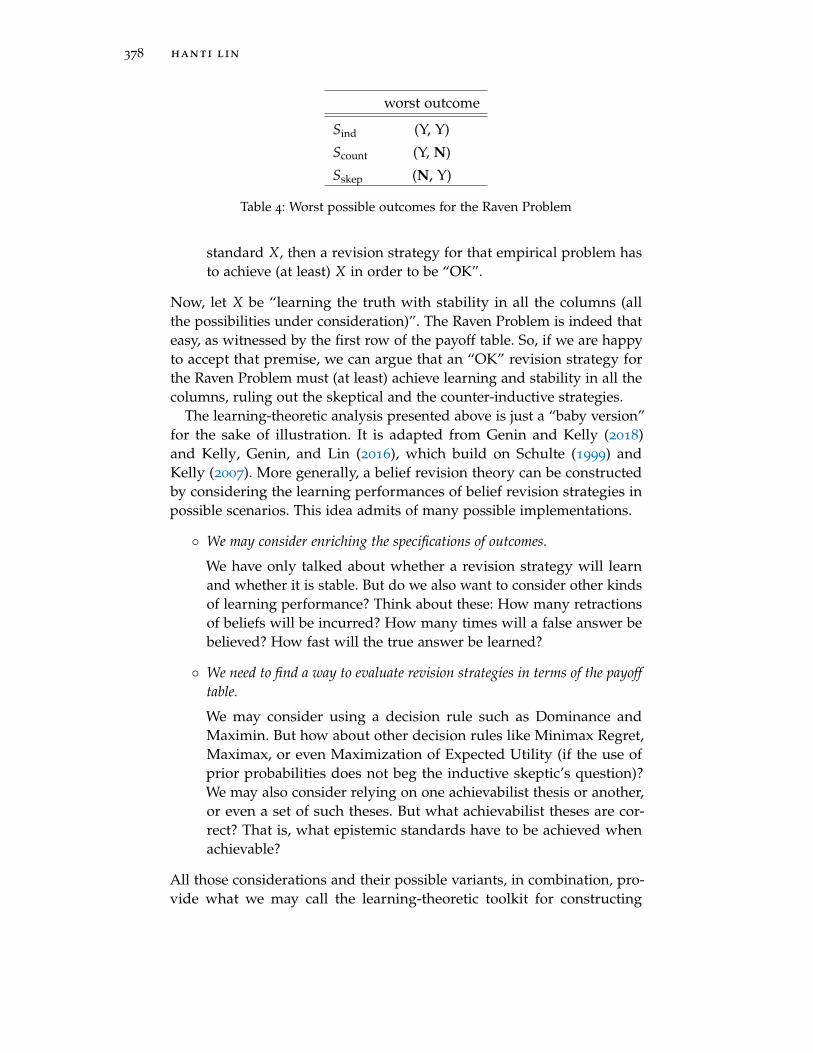
378 hanti lin
worst outcome
Sind (Y, Y)
Scount (Y, N)
Sskep (N, Y)
Table 4: Worst possible outcomes for the Raven Problem
standard X, then a revision strategy for that empirical problem hasto achieve (at least) X in order to be “OK”.
Now, let X be “learning the truth with stability in all the columns (allthe possibilities under consideration)”. The Raven Problem is indeed thateasy, as witnessed by the first row of the payoff table. So, if we are happyto accept that premise, we can argue that an “OK” revision strategy forthe Raven Problem must (at least) achieve learning and stability in all thecolumns, ruling out the skeptical and the counter-inductive strategies.
The learning-theoretic analysis presented above is just a “baby version”for the sake of illustration. It is adapted from Genin and Kelly (2018)and Kelly, Genin, and Lin (2016), which build on Schulte (1999) andKelly (2007). More generally, a belief revision theory can be constructedby considering the learning performances of belief revision strategies inpossible scenarios. This idea admits of many possible implementations.
We may consider enriching the specifications of outcomes.
We have only talked about whether a revision strategy will learnand whether it is stable. But do we also want to consider other kindsof learning performance? Think about these: How many retractionsof beliefs will be incurred? How many times will a false answer bebelieved? How fast will the true answer be learned?
We need to find a way to evaluate revision strategies in terms of the payofftable.
We may consider using a decision rule such as Dominance andMaximin. But how about other decision rules like Minimax Regret,Maximax, or even Maximization of Expected Utility (if the use ofprior probabilities does not beg the inductive skeptic’s question)?We may also consider relying on one achievabilist thesis or another,or even a set of such theses. But what achievabilist theses are cor-rect? That is, what epistemic standards have to be achieved whenachievable?
All those considerations and their possible variants, in combination, pro-vide what we may call the learning-theoretic toolkit for constructing

belief revision theory 379
various formal theories of belief revision. But which specific tools shouldwe use in order to construct a belief revision theory that has a plausiblenormative interpretation? This issue will be revisited in Section 6.3.
Also see Kelly (1999) for an application of learning-theoretic analysisto iterated belief revision, which considers the possibility of receivingmutually contradictory pieces of information.
The learning-theoretic analysis need not be a rival to the aforementionedapproaches to belief revision theory. Indeed, as we have seen, the learning-theoretic analysis is able to rule out some notable revision strategies, suchas the skeptical and counter-inductive strategies. This ability seems tocomplement the more standard, AGM belief revision theory: the skepticalstrategy is not ruled out by the AGM theory because it can be modeled bya complete order of relative plausibility that takes every possible worldto be equally plausible; the counter-inductive strategy is not ruled out bythe AGM theory, either, because it can also be modeled by an appropriatecomplete order of relative plausibility. Perhaps the right theory of beliefrevision should be constrained jointly by the learning-theoretic considera-tions and the considerations that follow, generalize, or weaken the AGMtheory. See Baltag, Gierasimczuk, and Smets (2016) and Genin and Kelly(2018) for more on the possibility of such a joint project.
4.7 Other Construction Techniques
There are many other techniques for constructing belief revision theories.Let me mention some of the most influential ones.
Instead of using plausibility orderings over possible worlds, we mayuse orderings over sentences, the so-called epistemic entrenchmentorderings (Gärdenfors & Makinson, 1988). This idea has been appliedto both simple belief revision and iterated belief revision (Nayak,1994).
On the approach of partial meet contraction, it is standardly assumedthat a belief set B be closed under logical consequence, but we mayrelax that assumption, letting B be a mere set of sentences, calleda belief base, on which the agent bases other beliefs (Hansson, 1994,1999).
If we think that almost all formal theories of simple belief revisionin the literature are too strong, we can resort to the standard trans-lation between simple belief revision and nonmonotonic inference(Makinson & Gärdenfors, 1991), which I present in the appendix(Section 8.1), and then translate a sufficiently weak nonmonotoniclogic into an equally weak theory of belief revision. The literature

380 hanti lin
of nonmonotonic logic does provide very weak systems, such asReiter’s (1980) default logic.18 When we translate Reiter’s defaultlogic into belief revision theory, the result is even weaker than systemP+, let alone AGM.19
Spohn (1988) proposes an approach to iterated belief revision theory,which considers belief revisions in situations of the following kind: anagent receives new information, but she is not fully certain whetherit is true, and somehow has a clear idea of how uncertain she issupposed to be, where the uncertainty in question is measured byordinal numbers. See the chapter on ranking theory (Huber, thisvolume).
For an extensive, detailed survey of construction techniques, see Rodrigueset al. (2011).
5 how to argue against
To argue against a normative theory of belief revision, the paradigmaticway is to provide intuitive counterexamples. But an alleged counterexam-ple usually raises a question: “Is that a genuine counterexample?” Let usthink about this issue by discussing concrete examples.
5.1 Three Composers Revisited
Recall the case of Three Composers, which we considered in Section 2.1.To facilitate cross reference, let me reproduce it below:
Example (Three Composers). Consider three composers: Verdi,Bizet, and Satie. The agent initially believes the following.
(A) Verdi is Italian;
(B) Bizet is French;
(C) Satie is French.
Then the agent receives this information.
(E) Verdi and Bizet are compatriots.
So she retains the belief in C that Satie is French (after all, informationE has nothing to do with Satie), but drops her beliefs in A and in B.Then the agent receives another piece of information.
(E′) Verdi and Satie are compatriots,
18 Reiter’s default logic is only one of the many approaches to nonmonotonic logic; seeBrewka, Niemelä, and Truszczynski (2008) for a review.
19 This observation is due to Makinson (1988).

belief revision theory 381
which is compatible with what she believes right before this newinformation arrives. Considering that she started with initial beliefsA, B, and C and has received two pieces of information E and E′,which jointly say that the three composers are compatriots, now shedrops her belief in C.
Let us recall that the second revision is an alleged counterexample toPreservation as a necessary condition of perfect rationality.
Anyone who wants to defend Preservation as a necessary conditionof perfect rationality may try responding in either of the following twoways. First, the defender may try explaining why the agent in the ThreeComposers case is actually irrational.
The second possible response proceeds as follows. E′ seems not the kindof thing that we can actually receive as new information. We would cometo believe E′ by inferring it from the new information that we can actuallyreceive, such as “my music teacher just told me that Verdi and Satie arecompatriots,” or “I just saw a chart coloring composers in terms of theirnationalities; it assigns the same color, red, to Verdi and Satie but I do notknow which nationality corresponds to red.” So the scenario misspecifiesthe new information that the agent actually receives. A realistic scenarioshould be more complicated than the one told above. So the above scenarioalso underspecifies how exactly the agent comes to gain the new belief inE′ and drop the old belief in C. The goal of this response is to show that,no matter how we retell the original Three Composers scenario in a wayfree from misspecification and underspecification, the retold story will notbe a counterexample to Preservation.20
To see how one may explain an alleged counterexample away by point-ing to underspecification or misspecification, let me provide other exam-ples in the following two subsections.
5.2 Underspecification
Katsuno and Mendelzon (2003) argue that the AGM theory is not univer-sally applicable. They propose the following counterexample.
Example (Book and Magazine). Suppose that the agent believesthat there is either a book on the table (B) or a magazine on the table(M), but not both. Consider two alternative developments of thisscenario:
Case 1: The agent is told that there is a book on the table. She thenconcludes B and ¬M.
20 I thank Horacio Arló-Costa for bringing this possible response to my attention.
382 hanti lin
Case 2: The agent is told that a book has been put on the table. Shethen concludes B but continues to suspend judgment about M.
So the agent starts by believing B∨M and ¬(B∧M). Katsuno and Mendel-zon agree that the AGM theory can easily explain Case 1 as follows: theagent receives information B and, hence, by the Accretion axiom in theAGM theory, she comes to believe ¬M. But Katsuno and Mendelzon thinkthat Case 2 is a counterexample to the Accretion axiom in the AGM theorybecause (i) the new information is compatible with the old beliefs and (ii)the new information plus the old beliefs entails ¬M, which the agent doesnot believe after the revision.
The lesson they want to draw is that we need a theory of belief revisionlike AGM to deal with Case 1, but we need a distinct theory, what theycall a theory of belief update, to deal with Case 2.
But the AGM theorist could respond by saying that Katsuno and Mendel-zon underspecify Case 2. Here is one possible way to specify Case 2 withsufficient detail.
Case 2’: The agent starts by believing not only that B ∨M and ¬(B ∧M) are both true at t0, but also that if a book is put on the table att1(> t0), then, first, B is true at t1 and, second, M is true at t0 iff Mis true at t1. Then the agent is told, at t1, that a book is indeed put onthe table at t1. In this case she should continue to suspend judgmentabout M.
Given this more detailed specification of Case 2, the AGM theorist can usethe Accretion axiom to explain why the agent should suspend judgmentabout M at t1. Note that the new information is consistent with the set ofher old beliefs. Furthermore, the new information plus the set of her oldbeliefs is silent about the truth value of M at t1 (and this is made clear byexplicit references to times t0 and t1). Therefore, by Accretion one shouldsuspend judgment about the truth value of M at t1.
So Katsuno and Mendelzon’s alleged counterexample does not reallyrefute the AGM theory. The lesson is that an alleged counterexample mayfail to work due to underspecification.
I want to make a second point. Belief revision theory is very inter-disciplinary, studied by philosophers, logicians, and computer scientists.There are people belonging to all the three groups, but there are alsopeople belonging to only one or two. So different belief revision theoristsmight have very different goals in mind when using counterexamples.A sympathetic reading of Katsuno and Mendelzon’s paper—a paper inartificial intelligence—suggests that they are interested in situations wherethe object language is so austere that it contains no tense operators orreferential expressions about time. So the conclusion they want to draw

belief revision theory 383
can be charitably understood as saying that, given that the object languageis so austere (and hence computationally easier to deal with), the AGMtheory when restricted to that language cannot accommodate Case 2. Thisconclusion should be very interesting to computer scientists: it wouldbe interesting to see if Case 2 can be accommodated by an algorithmthat manipulates a very simple language and implements a non-AGMbelief revision theory. It is just that this conclusion, although interesting incomputer science, is not equally interesting in epistemology.
5.3 Misspecification
Stalnaker (2009) argues against the following constraint on iterated beliefrevision.
Axiom C2 (Darwiche and Pearl, 1997). S(φ1, . . . , φn, α, β) =
S(φ1, . . . , φn, β), whenever the latest information β is incompatiblewith the preceding information α.
This says, roughly, that when one receives information α and then the nextpiece of information β contradicts α, one ought to revise beliefs as if onehad only received β without receiving α. Darwiche & Pearl’s Axiom C2 isamong the weakest studied in the belief revision literature. Indeed, it issatisfied by every revision strategy that always follows canonical revision(which is the weakest requirement of iterated belief revision discussed inSection 4.5). But Stalnaker (2009) proposes a counterexample to Axiom C2.
Example (Coin Flipping). A fair coin is flipped in each of the tworooms, 1 and 2. Alice and Bert (who I initially take to be reliable)report to me, independently, about the results: Alice tells me that thecoin in room 1 came up heads, while Bert tells me the same about thecoin in room 2. So I believe what they tell me at stage one. But thenCarla and Dora, also two independent witnesses whose reliability,in my view, trumps that of Alice and Bert, give me information thatconflicts with what I heard from Alice and Bert. Carla tells me thatthe coin in room 1 came up tails, and Dora tells me the same aboutthe coin in room 2. These two reports are given independently, andsimultaneously.21 This is stage two. Finally, stage three: Elmer, whosereliability trumps everyone else, tells me that that the coin in room1 in fact landed heads. (So Alice was right after all.) What should Inow believe about the coin in room 2?
21 This simultaneity assumption is crucial for Stalnaker’s purposes. Although this kind ofsimultaneity (relative to the agent’s frame of reference) is extremely rare, it is still possible.So this example is a genuine possibility.

384 hanti lin
It seems that the agent, at the final stage, should believe that the coin inroom 2 came up tails, for Elmer says nothing that contradicts what Dorasays. But this result, Stalnaker claims, violates Darwiche & Pearl’s AxiomC2. To see why, let:
α = the conjunction of what Carla says and what Dora says;
β = what Elmer says.
The latest information β contradicts the information α obtained at thepreceding stage, and it does so only because it contradicts the first conjunctof α (i.e. what Carla says). But Axiom C2 asks the agent to act as ifinformation α were not received at all and, hence, as if Dora’s testimonywere not received. By contrast, we seem to have the intuition that the agentshould retain her belief in what Dora says—after all, the latest informationβ does not undermine what Dora says. The problem with Axiom C2 seemsto be this: it requires that Dora’s testimony be discredited only because itarrived at the same time as someone else’s discredited testimony.
Those who want to defend Darwiche & Pearl’s Axiom C2 might respondthat Stalnaker actually misspecifies the information in question. The agentdoes not really receive any information whose content is that the coin inroom Y came up Z. The information received should be of this form: “agentX says that the coin in room Y came up Z.” That is, the real informationshould not be the content of what people say, but should report the factthat those people say such and such things. Then there is no contradictionbetween the earlier information and the later information in the CoinFlipping case, and hence there is no violation of Axiom C2—or so theresponse concludes.
So, if the above response is right, Stalnaker’s alleged counterexamplefails to work due to misspecification.
This hypothetical exchange between Stalnaker and the defender ofAxiom C2 raises a deep question. The clash between Stalnaker’s counterex-ample and the defender’s response can be taken as a debate over whatcounts as information, assuming that both parties employ the same concep-tion of information. But what if Stalnaker and the defender presupposedistinct conceptions of information? That is, what if they are talking pasteach other? This question points to a debate concerning the nature or goalof belief revision theory. According to the conception of information usedin Stalnaker’s specification of the scenario, the information that the agentreceives takes the form of E2 rather than E1.
(E1) Agent X says that the coin in room Y came up Z.(E2) The coin in room Y came up Z.
But according to another conception of information—the one used in theresponse—the agent only receives information of the form E1, while E2

belief revision theory 385
comes to be believed as a result of revising the agent’s old beliefs in light ofinformation E1. Now, if the two parties do presuppose distinct conceptionsof information, the real debate is this:
Choice among Conceptions of Information. Which conceptionof information should be the one used in belief revision theory?Or, without presupposing that there is a unique conception of in-formation to be used in belief revision theory, how should thoseconceptions of information play their respective roles in belief revi-sion theory?
These are difficult questions to answer. If we are going to have two concep-tions of information in belief revision theory, then we will have to rewritethe formal theories presented above, for they simply do not distinguishdifferent conceptions of information. If we are to stick with the morepermissive conception of information that Stalnaker has in mind, then itseems that we are developing a belief revision theory that does not addressan important kind of belief revision, i.e. the cases in which E2 is believedas a result of belief revision in light of information E1. But if, instead, weare to stick with the more restrictive conception of information, then wewill create a slippery slope. Which of the following is the information thatthe agent receives?
(E0) Agent X utters ‘the coin in room Y came up Z’.(E1) Agent X says that the coin in room Y came up Z.(E2) The coin in room Y came up Z.
If we want a restrictive conception that excludes E2 as information, why notgo for the most restrictive conception that allows only E0 as information,and take the other two to be something that the agent might come tobelieve by revising old beliefs in light of the sole information E0? And,if we really adopt such a restrictive conception of information, then itseems pointless to develop a theory of iterated belief revision that aspiresto take care of so many cases, including the cases in which one receivesinformation α and later receives information β that contradicts α. Thesecases would be made impossible or extremely rare by the most restrictiveconception of information.
So which conception(s) of information should we use in belief revisiontheory? That is a tough issue, not usually discussed by belief revision theo-rists. But Gärdenfors (1988), for example, does elaborate on the conceptionof information that he intends to work with.
We arrived at a foundational issue from an alleged counterexample to abelief revision theory. Discussions about counterexamples are importantbecause we may use them to refute theories, but also because they some-times raise deep questions concerning what exactly we want to theorizeabout.

386 hanti lin
6 how to argue for
Arguments for particular belief revision theories do not usually receiveexplicit formulations in the literature. But two argumentative approachesare discernible in the literature. On the first approach, one argues for abelief revision theory in terms of how well it survives alleged counterex-amples. On the second approach, a formal but motivated construction of abelief revision theory is somehow “transformed” into an argument for thetheory. Let me explain these two approaches in turn.
6.1 Argument from Surviving Alleged Counterexamples
We use intuitive examples to refute general theories. So a possible argu-ment schema we may use is the following.
(i) We have worked very diligently in search of intuitive counterexam-ples to this normative theory of belief revision but have not beenable to find a genuine counterexample.
(ii) Therefore, this theory is plausible.
This argument is certainly not valid, but perhaps it is harmless to make itvalid by adding a premise: if (i) then (ii).
That is the first approach we may adopt in order to argue for a beliefrevision theory, but hopefully not the only approach. We may have con-flicting intuitions about concrete examples. When we do, we will debateover premise (i). So it would be great to explore whether there are moretheoretical, general considerations that can help us resolve or mitigate ourdisagreement. That brings us to the second approach.
6.2 Argument from Construction: Partial Meet Contraction
On the second approach, a construction of a formal belief revision theoryis to be interpreted and then turned into an argument for a normativetheory of belief revision. I will illustrate with two construction techniques:first with partial meet contraction (in this subsection), and then with thelearning-theoretic analysis (in the next subsection).

belief revision theory 387
Belief revision theorists working on partial meet contraction seem tohave the following line of thought in mind. Recall that this constructiontechnique generates belief revision strategies S as follows:
S(φ) =(0) B ∗ φ
=(1) (B÷¬φ) + φ
=(2)⋂
γ(B⊥¬φ) + φ
=(3)⋂X ∈ B⊥¬φ : X ≥ Y for all Y ∈ B⊥¬φ + φ.
These equations jointly describe a formal procedure by which we can usea binary relation ≥ over sets of sentences to generate a belief revisionstrategy S. Under a suitable interpretation, this procedure may tell a storyabout a rational agent who is trying to revise beliefs, about the sensibleconsiderations that she has, and about the rational decisions that shemakes. In fact, this story was already sketched in Section 4.2, in which allformal apparatuses—ranging from ÷, ⊥, γ, to ≥—were introduced withmotivations. (Of course, there are details to be filled into the story sketchedin that section, and some parts of the story may require fine-tuning tomake the whole story plausible.) Some belief revision theorists such asGärdenfors (1984) do take the story—the interpreted formal procedure—very seriously, and they think that the story somehow lends plausibility tothe belief revision theory they construct.
The question I want to discuss here is how the above line of thoughtcan possibly be turned into an explicit argument with a clearly specifiednormative conclusion. Let us explore some possibilities. Suppose that theprocedure (0)–(3) of partial meet contraction has been given an interpreta-tion in line with the motivations provided in Section 4.2. Suppose, further,that the normative thesis to be argued for is the following.
Putative Conclusion. An agent is perfectly rational only if shehas been following, and would continue to follow, a belief revisionstrategy S that is constructible through procedure (0)–(3).
Note that this putative conclusion does not make the implausibly strongclaim that an agent is perfectly rational only if she actually follows proce-dure (0)–(3); there may be distinct procedures leading to the same finalproduct. Now add the following premise.
Premise (I). Procedure (0)–(3), under such and such an interpretation,describes a possible process for perfectly rational belief revision.
But the above premise alone does not suffice, for it only describes procedure(0)–(3) as one possible process for perfectly rational belief revision. Thisleaves us with the following open question.

388 hanti lin
Open Question. Is there a procedure that describes another possibleprocess for perfectly rational belief revision, but generates a beliefrevision strategy not constructible through procedure (0)–(3)?
If the answer is “yes,” then the putative conclusion is false. So, to makethe argument valid, we need to add at least the following premise (orsomething to the same effect).
Premise (II). The answer to the above question is “no.”
But this second premise is far from obvious, so an argument for it isrequired. Indeed, since procedure (0)–(3) is committed to Preservation,the Three Composers case is a potential counterexample to Premise (II).Perhaps one can try to argue that procedure (0)–(3) describes a very“paradigmatic” process for perfectly rational belief revision—so paradig-matic that the answer to the open question is “no,” and that the putativeconclusion must be true. It remains to explore how one may elaborate onthis line of thought.
So, for those who are sympathetic to the philosophical significance ofpartial meet contraction (0)–(3), a foundational issue in belief revisiontheory is how we may provide more premises besides (I) and produce asensible, valid argument for the putative conclusion.
But even if such an argument can be produced, Premise (I) can bechallenged. That is, one may challenge the very possibility of a workableinterpretation of procedure (0)–(3). Recall the main idea of this procedure.Suppose that one receives information φ, and that φ is incompatiblewith the set B of one’s old beliefs. Then some old beliefs have to beretracted before φ is added to one’s stock of beliefs. That is, before oneadds φ, one needs to find a contracted set B÷¬φ of beliefs, a subset of Bthat is compatible with φ. It is hypothesized that one should not retractbeyond necessity (but why?).22 So let the agent consider all elements ofthe remainder set B⊥¬φ, i.e. all inclusion-maximal subsets of B that arecompatible with φ. Then let relation ≥ sort out the “best” of those subsets.The intersection of those best subsets,
⋂X ∈ B⊥¬φ : X ≥ Y for all Y ∈B⊥¬φ, is then identified with the contracted set of beliefs, B÷¬φ. That’sthe main idea. But that raises an issue concerning the right interpretationof ≥. Let us try the following interpretation:
Interpretation of ≥ (1). X ≥ Y means that X is at least as good asY as a candidate for B÷¬φ.
Under this interpretation, the intersection of the “best” candidates forB÷¬φ (“best” with respect to ≥) may not be a “best” candidate for B÷¬φ
(“best,” again, with respect to ≥). So a non-optimal candidate may be
22 For more on this issue, see Rott (2000).

belief revision theory 389
selected! So this particular interpretation of X ≥ Y makes the constructionprocess incoherent: one does not choose from the best candidates, but optsfor the intersection of the best candidates, which may be sub-optimal.
What else could X ≥ Y mean? Let us try Gärdenfors’ (1984) suggestion:
Interpretation of ≥ (2). X ≥ Y means that X is epistemically atleast as “important” as Y.
Following this interpretation, procedure (0)–(3) assumes that the contractedbelief set B ÷ ¬φ must be the intersection of the most “epistemicallyimportant” elements of B⊥¬φ. Gärdenfors’ interpretation of ≥ does notcause any incoherence, but he leaves us with some unanswered questions.First, how should we understand the concept that Gärdenfors refers toas epistemic importance? Second, why should the contracted belief setbe the intersection of the epistemically most important candidates? Thatis, why are the concepts of belief contraction and epistemic importancenormatively related that way? Plausible answers to these questions arerequired if we want to use Gärdenfors’ interpretation of ≥ to defendPremise (I) and, ultimately, to argue for the putative conclusion listedabove.
So there are a number of issues to address if we want to take seriouslythe construction of partial meet contraction and turn it into an explicitargument. For more on how we may take partial meet contraction seriously,see Gärdenfors (1984), Levi (2004), and Arló-Costa and Levi (2006).
6.3 Argument from Construction: Learning-Theoretic Analysis
Let us examine another technique for constructing belief revision theories:learning-theoretic analysis. Recall that this construction selects belief re-vision strategies according to some decision rule or achievabilist thesis(Section 4.6). This suggests the following argument schema, where T is aformal theory of belief revision, i.e. a set of revision strategies.
Premise (I). J (as a decision rule or achievabilist thesis) judges astrategy to be not “OK” if that strategy is not in T.
Premise (II). If J judges a strategy to be not “OK”, then that strategyis not rational (or epistemically justified, or the like).
Putative Conclusion. Therefore, a strategy is rational (or epistemi-cally justified, or the like) only if it is in T.
A candidate for J is the Dominance principle, as mentioned in Section 4.6.When outcomes, or learning performances, are specified in greater detail,it is likely that only very few strategies are dominated. Indeed, a general

390 hanti lin
feature of the Dominance principle is that it becomes weaker when out-comes are specified in greater detail. So, in general, it would be difficult touse the dominance principle to argue for a strong normative thesis.
In that case, one might consider resorting to another candidate forJ mentioned in Section 4.6: the Maximin decision rule. But there is alongstanding worry that, in many situations, the Maximin rule is toopessimistic to be the right rule to apply. Indeed, the dominant view indecision theory is that a correct decision rule has to involve one’s degreesof belief over the columns in the decision table, rather than (pessimistically)focusing on the worst possible outcomes. There is a possible response infavor of applying Maximin to some contexts. The learning-theoretic anal-ysis is actually developed to address the so-called problem of induction.Namely, it is meant to respond to the inductive skeptic’s questions: “Howcan we justify induction?” “How can we justify inductive strategies ratherthan skeptical strategies?” “How can we justify the use of a particularinductive strategy rather than an alternative inductive strategy?” To prop-erly address these tough questions, we cannot rely on anyone’s degreesof belief over the columns in the decision table, for fear of begging theskeptic’s question—or so Lange (2002) argues. So, to make a decisionwithout begging the skeptic’s question, the right decision rule, if there isone, has to be a qualitative decision rule. And the Maximin rule seems agood candidate—or so this response suggests and promises to elaborate.This idea, which favors the use of Maximin in some contexts, may betraced at least back to the Maximin foundation of statistical inference dueto Wald (1950). Note that those sympathetic to the above line of thought donot have to stick with Maximin but can switch to, and argue for, anotherqualitative decision rule that does not presuppose degrees of belief. Kelly(2007), for example, proposes a kind of dominance principle that appliesto the worst-case bounds of “complexity classes”—a decision rule inspiredby how computer scientists evaluate the efficiency of problem-solvingalgorithms.
There is another kind of candidate for J mentioned in Section 4.6,achievabilist theses, which take this form: “If the empirical problem inquestion is easy enough to allow a revision strategy to achieve epistemicstandard X, then a revision strategy for that empirical problem is “OK”only if it achieves (at least) X.” Achievabilist theses have seldom beenformulated explicitly in learning theory, and they seem to be central to theway Putnam (1965) and Gold (1967) created formal learning theory in the1960’s—or so Kelly (1996) seems to suggest. But which achievabilist thesesare correct and how should they be defended or at least motivated? Therehave been very few systematic discussions on this issue in the literature,but see Kelly et al. (2016) and Genin and Kelly (2018) for examples of

belief revision theory 391
how certain epistemic standards may be motivated and put to use inachievabilist theses.
7 concluding remarks
We have discussed a number of foundational issues about belief revisiontheory. Let us recap what we have covered. Have a look at the italicizedterms below.
A belief revision theory is meant to make normative or evaluative(i)claims(ii) about revision of beliefs in light of new information(iii).
With respect to (i), we have noted that alternative normative interpretationscan be given to a formal belief revision theory, and have seen that the choiceamong those possible interpretations amounts to the choice among verydifferent research programs in belief revision theory (Section 2.3). Withrespect to (ii), we have examined some methods that we may use to arguefor or against the normative claims that a belief revision theory is intendedto make (Section 5 and Section 6), including various potential difficulties orissues that we need to address when trying to apply those argumentativemethods. With respect to (iii), we have only briefly discussed the issue ofwhat counts as information and the problem of choosing among differentconceptions of information (Section 5.3).
For discussions of other philosophical issues, see Levi (1983), Levi (1991),Levi (2004), Gärdenfors (1988), Rott (2000), Rott (2001), Hansson (1999),Hansson (2003), Gillies (2004), and Genin and Kelly (2018).
8 appendix
8.1 Nonmonotonic Logic and Belief Revision Theory
A nonmonotonic consequence relation is a binary relation |∼ between sen-tences. Understand φ |∼ψ as saying of |∼ that it licenses the inference fromφ to ψ—a possibly defeasible, inductive, or plausible inference. Nonmono-tonic logic, if broadly construed, aims at distinguishing nonmonotonicconsequence relations that are good in one sense or another. There aremany approaches to nonmonotonic logic; they differ in the proceduresthat are used to sort out “good” nonmonotonic consequence relations; seeBrewka et al. (2008) for a review.
Makinson and Gärdenfors (1991) propose a translation between simplebelief revision strategies S and nonmonotonic consequence relations |∼ .

392 hanti lin
Their translation is based on the following bridge principle (which I statein terms of the S-notation used here):
ψ ∈ S(φ) iff φ |∼ψ.
To be more precise: given any simple belief revision strategy S, we canuse the bridge principle to define a nonmonotonic consequence relation|∼S as follows: φ |∼Sψ iff ψ ∈ S(φ). Conversely, given any nonmonotonic
consequence relation |∼ , we can use the bridge principle to define asimple belief revision strategy S |∼ as follows: S |∼(φ) =def ψ : φ |∼ψ andS |∼() =def S |∼(>), where > is a tautology.
This establishes a one-to-one correspondence between all nonmonotonicconsequence relations and all simple belief revision strategies S such thatS() = S(>).
8.2 General Definition of Learning
Let an information space I be given, which contains some finite sequencesof sentences, meant to represent possible available pieces of information. Leta question Q be identified with a set of mutually incompatible sentences,called the potential answers to Q. The potential answers to Q may, or maynot, be jointly exhaustive—let the disjunction of the potential answersto Q be understood as the presupposition of question Q. Let a decisiontable be given, together with a set C of columns as mutually incompatiblepossibilities. Those columns/possibilities are assumed to be so specificthat each column C ∈ C either entails exactly one potential answer toquestion Q or it entails the negation of Q’s presupposition. With respectto the above setting (Q, I , C), define the following concepts.
An I-information stream is an infinite sequence (φ1, φ2, . . .) of sen-tences such that its finite initial segments are all in I .
Say that an I-information stream (φ1, φ2, . . .) is compatible with acolumn C ∈ C iff the infinite conjunction
∧i≥1 φi is compatible with
possibility C.
The true answer to question Q given column C, written Ans(Q | C),is defined as the unique potential answer to Q that C entails, if sucha unique answer exists; otherwise, Ans(Q | C) is undefined.
We are finally in a position to define learning with respect to the abovesetting.
Say that a strategy S will learn the true answer to question Q givencolumn C just in case:

belief revision theory 393
(1) the true answer Ans(Q | C) exists;
(2) for each I-information stream (φ1, φ2, . . .) compatible with C,there exists n ≥ 1, called a “learning moment,” such that foreach i ≥ n, S(φ1, φ2, . . . , φi) is consistent and entails Ans(Q | C).
acknowledgements
I am indebted to Kevin Kelly and Horacio Arló-Costa for teaching me somuch about belief revision theory. This article would have been impossiblewithout them. I am indebted to the two editors, Jonathan Weisberg andRichard Pettigrew, for their endless patience and very helpful comments. Iam also indebted to Ted Shear for his incredibly detailed comments anduseful suggestions, and to Kasey Genin, Jake Chandler, Adam Sennet, andRachel Boddy for their stimulating questions.
references
Alchourrón, C. E., Gärdenfors, P., & Makinson, D. (1985). On the logic oftheory change: Partial meet contraction and revision functions. Thejournal of symbolic logic, 50(2), 510–530.
Arló-Costa, H. & Levi, I. (2006). Contraction: On the decision-theoreticalorigins of minimal change and entrenchment. Synthese, 152(1), 129–154.
Arló-Costa, H. & Pedersen, A. P. (2012). Belief and probability: A gen-eral theory of probability cores. International Journal of ApproximateReasoning, 53(3), 293–315.
Baltag, A., Gierasimczuk, N., & Smets, S. (2016). On the solvability ofinductive problems: A study in epistemic topology. arXiv preprintarXiv:1606.07518, presented at the 2015 TARK.
Booth, R. & Chandler, J. (2017). The irreducibility of iterated to singlerevision. Journal of Philosophical Logic, 46(4), 405–418.
Boutilier, C. (1996). Iterated revision and minimal change of conditionalbeliefs. Journal of Philosophical Logic, 25(3), 263–305.
Brewka, G., Niemelä, I., & Truszczynski, M. (2008). Nonmonotonic reason-ing. Foundations of Artificial Intelligence, 3, 239–284.
Darwiche, A. & Pearl, J. (1997). On the logic of iterated belief revision.Artificial intelligence, 89(1-2), 1–29.
Gärdenfors, P. (1984). Epistemic importance and minimal changes of belief.Australasian Journal of Philosophy, 62(2), 136–157.
Gärdenfors, P. (1988). Knowledge in flux: Modeling the dynamics of epistemicstates. The MIT press.

394 hanti lin
Gärdenfors, P. & Makinson, D. (1988). Revisions of knowledge systemsusing epistemic entrenchment. In Proceedings of the 2nd conferenceon theoretical aspects of reasoning about knowledge (pp. 83–95). MorganKaufmann Publishers Inc.
Genin, K. (2019). Full & partial belief. In R. Pettigrew & J. Weisberg (Eds.),The open handbook of formal epistemology. PhilPapers.
Genin, K. & Kelly, K. T. (2018). Theory choice, theory change, and inductivetruth-conduciveness. Studia Logica. doi:10.1007/s11225-018-9809-5
Gillies, A. S. (2004). Epistemic conditionals and conditional epistemics.Noûs, 38(4), 585–616.
Ginsberg, M. L. (1986). Counterfactuals. Artificial intelligence, 30(1), 35–79.Gold, E. M. (1967). Language identification in the limit. Information and
control, 10(5), 447–474.Grove, A. (1988). Two modellings for theory change. Journal of philosophical
logic, 17(2), 157–170.Hansson, S. O. (1994). Taking belief bases seriously. In Logic and philosophy
of science in uppsala (pp. 13–28). Springer.Hansson, S. O. (1999). A textbook of belief dynamics. Springer Science &
Business Media.Hansson, S. O. (2003). Ten philosophical problems in belief revision. Journal
of logic and computation, 13(1), 37–49.Hansson, S. O. (2017). Logic of belief revision. In E. N. Zalta (Ed.), The Stan-
ford encyclopedia of philosophy (Winter 2017). Metaphysics ResearchLab, Stanford University.
Harper, W. L. (1975). Rational belief change, popper functions and coun-terfactuals. Synthese, 30(1-2), 221–262.
Harper, W. L. (1976). Rational conceptual change. In Psa: Proceedings ofthe biennial meeting of the philosophy of science association (Vol. 1976, 2,pp. 462–494). Philosophy of Science Association.
Huber, F. (2013a). Belief revision i: The agm theory. Philosophy Compass,8(7), 604–612.
Huber, F. (2013b). Belief revision ii: Ranking theory. Philosophy Compass,8(7), 613–621.
Huber, F. (2019). Ranking theory. In R. Pettigrew & J. Weisberg (Eds.), Theopen handbook of formal epistemology. PhilPapers.
Jin, Y. & Thielscher, M. (2007). Iterated belief revision, revised. ArtificialIntelligence, 171(1), 1–18.
Katsuno, H. & Mendelzon, A. O. (2003). On the difference between updat-ing a knowledge base and revising it1. Belief revision, 29, 183.
Kelly, K. T. (1996). The logic of reliable inquiry. Oxford University Press.Kelly, K. T. (1999). Iterated belief revision, reliability, and inductive amnesia.
Erkenntnis, 50(1), 7–53.

belief revision theory 395
Kelly, K. T. (2007). How simplicity helps you find the truth withoutpointing at it. In Induction, algorithmic learning theory, and philosophy(pp. 111–143). Springer.
Kelly, K. T., Genin, K., & Lin, H. (2016). Realism, rhetoric, and reliability.Synthese, 193(4), 1191–1223.
Kraus, S., Lehmann, D., & Magidor, M. (1990). Nonmonotonic reasoning,preferential models and cumulative logics. Artificial intelligence, 44(1-2), 167–207.
Lange, M. (2002). Okasha on inductive scepticism. The Philosophical Quar-terly, 52(207), 226–232.
Leitgeb, H. (2014). The stability theory of belief. The Philosophical Review,123(2), 131–171.
Levi, I. (1978). Subjunctives, dispositions and chances. In Dispositions(pp. 303–335). Springer.
Levi, I. (1983). The enterprise of knowledge: An essay on knowledge, credalprobability, and chance. MIT press.
Levi, I. (1991). The fixation of belief and its undoing: Changing beliefs throughinquiry. Cambridge University Press.
Levi, I. (2004). Mild contraction: Evaluating loss of information due to loss ofbelief. Oxford University Press on Demand.
Lin, H. & Kelly, K. T. (2012). Propositional reasoning that tracks probabilis-tic reasoning. Journal of philosophical logic, 41(6), 957–981.
Makinson, D. (1988). General theory of cumulative inference. In Interna-tional workshop on non-monotonic reasoning (pp. 1–18). Springer.
Makinson, D. & Gärdenfors, P. (1991). Relations between the logic oftheory change and nonmonotonic logic. In The logic of theory change(pp. 183–205). Springer.
Nayak, A. C. (1994). Iterated belief change based on epistemic entrench-ment. Erkenntnis, 41(3), 353–390.
Nute, D. (2012). Defeasible deontic logic. Springer Science & Business Media.Putnam, H. (1965). Trial and error predicates and the solution to a problem
of mostowski. The Journal of Symbolic Logic, 30(1), 49–57.Quine, W. V. O. (1982). Methods of logic. Harvard University Press.Reiter, R. (1980). A logic for default reasoning. Artificial intelligence, 13(1-2),
81–132.Rodrigues, O., Gabbay, D., & Russo, A. (2011). Belief revision. In Handbook
of philosophical logic (pp. 1–114). Springer.Rott, H. (1993). Belief contraction in the context of the general theory of
rational choice. The Journal of Symbolic Logic, 58(4), 1426–1450.Rott, H. (2000). Two dogmas of belief revision. The Journal of Philosophy,
97(9), 503–522.Rott, H. (2001). Change, choice and inference: A study of belief revision and
nonmonotonic reasoning. Clarendon Press.
396 hanti lin
Schulte, O. (1999). Means-ends epistemology. The British Journal for thePhilosophy of Science, 50(1), 1–31.
Shoham, Y. (1987). A semantical approach to nonmonotonic logics. InReadings in nonmonotonic reasoning (pp. 227–250). Morgan KaufmannPublishers Inc.
Spohn, W. (1988). Ordinal conditional functions: A dynamic theory ofepistemic states. In W. L. Harper & B. Skyrms (Eds.), Causation indecision, belief change and statistics: Proceedings of the irvine conferenceon probability and causation (pp. 105–134). The University of WesternOntario Series in Philosophy of Science. Kluwer.
Stalnaker, R. (1994). What is a nonmonotonic consequence relation? Fun-damenta Informaticae, 21(1, 2), 7–21.
Stalnaker, R. (2009). Iterated belief revision. Erkenntnis, 70(2), 189–209.Titelbaum, M. G. (2019). Precise credences. In R. Pettigrew & J. Weisberg
(Eds.), The open handbook of formal epistemology. PhilPapers.Wald, A. (1950). Statistical decision functions.

8R A N K I N G T H E O RY Franz Huber
In epistemology ranking theory is a theory of belief and its revision.It studies how an ideal doxastic agent should organize her beliefs andconditional beliefs at a given moment in time, and how she should reviseher beliefs and conditional beliefs across time when she receives newinformation. In this entry I will first present some background, mostnotably the AGM theory of belief revision (Alchourrón, Gärdenfors, &Makinson, 1985). In order to motivate the introduction of ranking theory Iwill then focus on the problem of iterated belief revisions. After presentingthe elements of ranking theory (Spohn, 1988, 2012) I will show how thistheory solves the problem of iterated belief revisions. I will conclude bysketching two areas of future research and by mentioning applicationsof ranking theory outside epistemology. Along the way we will see howranking theory, a theory of belief, compares to subjective probability theoryor Bayesianism, which is a theory of partial beliefs or degrees of belief.
1 introduction
Sophia believes many things, among others that it will rain on Tuesday,that it will be sunny on Wednesday, and that weather forecasts are alwaysright. Belief revision theory tells Sophia how to revise her beliefs whenshe learns that the weather forecast for Tuesday and Wednesday predictsrain. As we will see, this depends on the details of her beliefs, but underone way of filling in the details she should keep her belief that it will rainon Tuesday and give up her belief that it will be sunny on Wednesday. Tostate in full detail how Sophia should revise her beliefs when she learnsnew information we need a representation of her old beliefs and of thenew information she receives.
In this entry I will focus on ideal doxastic agents who do not sufferfrom the computational and other physical limitations of ordinary doxasticagents such as people and computer programs. These ideal doxastic agentsget to voluntarily decide what to believe (and to what degree of numericalprecision); they never forget any of their (degrees of) beliefs; and theyalways believe all logical and conceptual truths (to a maximal degree).We may perhaps define a (doxastic or cognitive) agent to be ideal just incase any (cognitive) action that is physically possible is an action that ispossible for her. Such ideal agents ought to do exactly that which theyought to do if they could, where the ‘can’ that is hidden in the ‘could’
397

398 franz huber
expresses possibility for the agent, not metaphysical possibility. Hence theprinciple that Ought Implies Can does not put any constraints on what anideal agent should do, and on what an ideal doxastic agent should believe.
Belief revision theory models belief as a qualitative attitude towardssentences or propositions: the ideal doxastic agent believes a proposition,or she disbelieves the proposition by believing its negation, or she sus-pends judgment with respect to the proposition and its negation. Thisis different from the theory of subjective probabilities, also known asBayesianism (Easwaran 2011a, 2011b; Titelbaum, this volume; Weisberg2011; Wenmackers, this volume), where belief is modeled as a quantita-tive attitude towards a proposition: the ideal doxastic agent believes aproposition to a specific degree, her degree of belief, or credence, for theproposition. However, we will see that, in order to adequately model con-ditional beliefs and iterated belief revisions, ranking theory also modelsthe ideal agent’s doxastic state with numbers, and thus more than just theset of propositions she believes. Genin (this volume) discusses the relationbetween belief and degree of belief.
2 belief revision
Spohn (1988, 1990) develops ranking theory in order to fix a problemthat besets the AGM theory of belief revision. In order to provide somebackground for ranking theory I will first present the AGM theory. Rankingtheory will then arise naturally out of the AGM theory. The latter theoryderives its name from the seminal paper by Alchourrón et al. (1985).Comprehensive overviews can be found in Gärdenfors (1988), Gärdenforsand Rott (1995), Rott (2001), and Lin (this volume).
One version of the AGM theory of belief revision represents the idealdoxastic agent’s old beliefs, her doxastic state at a given moment in time, bya set of sentences from some formal language, her belief set, together withan entrenchment ordering over these sentences. The entrenchment orderingrepresents how firmly the ideal doxastic agent holds the beliefs in herbelief set. It represents the details of the ideal agent’s doxastic state. Thenew information is represented by a single sentence. The AGM theorydistinguishes between the easy case, called expansion, and the general case,called revision. In expansion the new information does not contradict theideal doxastic agent’s old belief set and is simply added. In revision thenew information may contradict the ideal doxastic agent’s old belief set.The general case of revision is difficult, because the ideal doxastic agenthas to turn her old belief set, which is assumed to be consistent, into a newbelief set that contains the new information and is consistent. Usually thegeneral case is dealt with in two steps. In a first step, called contraction, theold belief set is cleared of everything that contradicts the new information.

ranking theory 399
In a second step one simply expands by adding the new information. Thismeans that the difficult doxastic task is handled by contraction, whichturns the general case of revision into the easy case of expansion.
A formal language L is defined inductively, or recursively, as follows. Lcontains the contradictory sentence p⊥q and all elements of a countableset of propositional variables PV = pPq, pQq, pRq, . . .. Furthermore,whenever A and B are sentences of L, then so are the negations of A andof B, p¬Aq and p¬Bq, respectively, as well as the conjunction of A and B,p(A ∧ B)q. Finally, nothing else is a sentence of L. The new informationis represented by a single sentence A from L. The ideal agent’s doxasticstate is represented by a set of sentences, her belief set B ⊆ L, plusan entrenchment ordering for B. The entrenchment ordering, whichrepresents the details of the ideal doxastic agent’s beliefs, orders theagent’s beliefs according to how reluctant she is to give them up: the moreentrenched a belief, the more reluctant she is to give it up.
The entrenchment ordering does most of the work in a revision of theagent’s beliefs. Suppose the agent receives new information that contra-dicts her belief set. Since the new belief set that results from the revisionhas to be consistent, some of the old beliefs have to go. The entrenchmentordering determines which beliefs have to go first: the least entrenched be-liefs are the beliefs that have to go first. If giving up those is not enough torestore consistency, the beliefs that are next in the entrenchment orderinghave to go next. And so on. The beliefs that would be given up last are themost entrenched ones. According to Maximality, they are the tautologicalsentences, which are always believed and never given up, because doing socannot restore consistency. On the other end of the spectrum are the leastentrenched sentences. According to Minimality, they are the sentences theagent does not even believe to begin with. These sentences do not belongto the agent’s belief set and so are gone before the revision process haseven begun.
If one sentence logically implies another sentence, then, according toDominance, the latter cannot be more entrenched than the former, asgiving up the belief in the latter sentence is to also give up the belief inthe former sentence. Dominance implies that the entrenchment orderingis reflexive: every sentence is at least as entrenched as itself. According toConjunctivity, two sentences cannot both be more entrenched than theirconjunction: one cannot give up one’s belief in a conjunction withoutgiving up one’s belief in at least one of the conjuncts. In combinationwith Dominance, Conjunctivity implies that the entrenchment orderingis connected: any two sentences can be compared to each other in termsof their comparative entrenchment. That is, either the first sentence is atleast as entrenched as the second sentence, or the second sentence is atleast as entrenched as the first sentence, or both. Finally, to ensure that the
400 franz huber
entrenchment ordering is a well-behaved ordering relation, it is assumedto be transitive by Transitivity.
More precisely, where ` is the logical consequence relationship on Land Cn (B) = A ∈ L : B ` A is the set of logical consequences of B(and ∅ is the empty set ), the entrenchment ordering has to satisfy thefollowing postulates. For all sentences A, B, and C from L:
1. If A B and B C, then A C. Transitivity
2. If A ` B, then A B. Dominance
3. A A ∧ B or B A ∧ B. Conjunctivity
4. Suppose B 6` ⊥. Then A /∈ B if, and only if,for all B ∈ L: A B. Minimality
5. If A B for all A ∈ L, then ∅ ` B. Maximality
The work that is done by the entrenchment ordering in a revision ofthe agent’s beliefs can also be described differently in terms of expansion,revision, and contraction, which turn belief sets and new informationinto belief sets (see Caie, this volume). Formally they are functions from℘(L)×L into ℘(L).
Expansion + turns each old belief set B ⊆ L and each sentence Afrom L into a new belief set B+A = Cn (B ∪ A). This is the easy casedescribed earlier about which there is little more to be said.
The difficult and more interesting case is revision ∗, which turns eachold belief set B ⊆ L and each sentence A from L into a new belief setB ∗ A. The operator ∗ is required to satisfy a number of postulates.
Closure requires revised belief sets to be closed under the logical conse-quence relation: after the revision is completed, the agent ought to believeall (and only) the logical consequences of the revised belief set. Congru-ence is similar in spirit to Closure and requires that it is the content of thenew information received, and not its particular formulation, that deter-mines what is added, and what is removed, from the agent’s belief set ina revision. Success requires that revising a belief set by new informationsucceeds in adding the new information to the agent’s belief set—and,given Closure, all sentences it logically implies. Consistency requires therevised belief set to be consistent as long as the new information is consis-tent. The remaining postulates all formulate different aspects of the ideathat, when revising her belief set by new information, the agent shouldadd and remove as few beliefs as possible from her belief set, subject tothe constraints that the resulting belief set is consistent and that the newinformation has been added successfully.
Inclusion requires that revising a belief set does not create any newbeliefs that are not also created by simply adding the new information. In

ranking theory 401
a sense it says that expansion is a special case of revision. Preservationrequires that revising a belief set by new information that does not con-tradict the agent’s old belief set does not lead to the loss of any beliefs.Conjunction 1 requires that, when revising her belief set by a conjunction,the agent adds only beliefs that she also adds when first revising her beliefset by one of the two conjuncts, and then adding the second conjunct.Conjunction 2 requires that, when revising her belief set by a conjunction,the agent adds all beliefs that she adds when first revising her belief set byone of the two conjuncts, and then adding the second conjunct—providedthe second conjunct is consistent with the result of revising her belief setby the first conjunct. More precisely, a revision function has to satisfy thefollowing postulates. For all sets of sentences B ⊆ L and all sentences Aand B from L:
∗1. B ∗ A = Cn (B ∗ A). Closure
∗2. A ∈ B ∗ A. Success
∗3. B ∗ A ⊆ Cn (B ∪ A). Inclusion
∗4. If B 6` ¬A, then B ⊆ B ∗ A. Preservation
∗5. If A ` B and B ` A, then B ∗ A = B ∗ B. Congruence
∗6. If ∅ 6` ¬A, then ⊥ 6∈ B ∗ A. Consistency
∗7. B ∗ (A ∧ B) ⊆ Cn((B ∗ A) ∪ B
). Conjunction 1
∗8. If ¬B 6∈ B ∗ A, thenCn((B ∗ A) ∪ B
)⊆ B ∗ (A ∧ B). Conjunction 2
The two-step view of revision described previously is known as the Leviidentity (Levi, 1977). It has the ideal doxastic agent first contract .− herold belief set B by the negation of the new information, ¬A, thus makingit consistent with the new information (as well as everything logicallyimplied by the new information). Then it has her expand the result B .−¬Aby adding the new information A:
B ∗ A = Cn((B .−¬A) ∪ A
).
The Levi identity puts contraction center stage in the revision process.Contraction .− turns each old belief set B ⊆ L and each sentence A from Linto a “reduced” belief set B .− A that is cleared of A as well as everythinglogically implying A. It is required to satisfy the following postulates. Forall sets of sentences B ⊆ L and all sentences A and B from L:
.−1. B .− A = Cn (B .− A). Closure

402 franz huber
.−2. If ∅ 6` A, then A 6∈ Cn (B .− A). Success
.−3. B .− A ⊆ Cn (B). Inclusion
.−4. If B 6` A, then B .− A = B. Vacuity
.−5. If A ` B and B ` A, then B .− A = B .− B. Congruence
.−6. Cn (B) ⊆ Cn((B .− A) ∪ A
). Recovery
.−7. (B .− A) ∩ (B .− B) ⊆ B .− (A ∧ B). Conjunction 1
.−8. If A 6∈ B .− (A ∧ B), then B .− (A ∧ B) ⊆ B .− A. Conjunction 2
Closure requires contracted belief sets to be closed under the logicalconsequence relation: after the contraction is completed, the agent oughtto believe all (and only) the logical consequences of the contracted belief set.Congruence is similar in spirit to Closure and requires that it is the contentof the sentence to be removed, and not its particular formulation, thatdetermines what is removed from the agent’s belief set in a contraction.Success requires that contracting a belief set by a sentence that is nottautological succeeds in removing this sentence from a belief set—and,given Closure, all sentences logically implying it. Inclusion requires thatcontracting a belief set does not add any beliefs to the belief set. Theremaining postulates all formulate different aspects of the idea that, whencontracting her belief set by a sentence, the agent should remove as fewbeliefs as possible from her belief set, subject to the constraints that theresulting belief set is consistent and that the sentence to be removed,together with all sentences logically implying it, is removed successfully.
Vacuity requires that contracting a belief set by a sentence leaves thebelief set unchanged if the sentence that was to be removed was not evenpart of the belief set to begin with. Recovery requires that contracting abelief set by a sentence removes as few beliefs as possible so that addingthe removed sentence again afterwards allows the agent to recover all herpreviously removed beliefs. Conjunction 1 requires that, when contractingher belief set by a conjunction, the agent does not remove any beliefs thatshe does not also remove when contracting by one or the other of the twoconjuncts alone. Finally, Conjunction 2 requires the following: if a conjunctis removed in contracting a belief set by a conjunction, then no belief getsremoved in contracting the belief set by this conjunct that does not alsoget removed in contracting this belief set by the entire conjunction. Theidea behind the last two postulates is that giving up one of its conjunctsis all the ideal doxastic agent needs to do in order to give up an entireconjunction.
The Levi identity turns each contraction operator .− satisfying .−1 – .−8into a revision operator ∗ satisfying ∗1 – ∗8. The converse is true of the

ranking theory 403
Harper identity (Harper, 1976). The latter has the ideal doxastic agent firstrevise the old belief set B by the negation of the new information, ¬A.Then it has her remove everything from the result B ∗ ¬A that was notalready also a logical consequence of the old belief set B:
B .− A = (B ∗ ¬A) ∩ Cn (B) .
If we have a belief set B ⊆ L we can use an entrenchment ordering forB to define a revision operator ∗ for L as follows. For every sentence Afrom L:
B ∗ A = Cn (B ∈ L : ¬A ≺ B ∪ A) ,
where A ≺ B holds if, and only if, A B and B 6 A.The idea behind this equation is the following. When the ideal doxastic
agent revises ∗ her old belief set B by the new information A she firsthas to clear B of ¬A as well as everything else that is as entrenchedas, or less entrenched than, ¬A. For instance, B also has to be clearedof everything that logically implies ¬A. However, it follows from thedefinition of an entrenchment ordering that all sentences B from the idealdoxastic agent’s old belief set B that are more entrenched than ¬A canbe preserved. This gives us the “preserved” belief set B ∈ L : ¬A ≺ B.Then the ideal doxastic agent adds the new information A to obtainB ∈ L : ¬A ≺ B ∪ A. Finally she adds all sentences that are logicallyimplied by the preserved belief set together with the new information. Asshown by Gärdenfors (1988) and Gärdenfors and Makinson (1988) one canthen prove
Theorem 1 Let L be a formal language. For each set of sentences B ⊆ L andeach entrenchment ordering for B satisfying 1 – 5 there is a revisionoperator ∗ from B×L into ℘ (L) satisfying ∗1 – ∗8 restricted to B such thatfor all A ∈ L:
B ∗ A = Cn (B ∈ L : ¬A ≺ B ∪ A) .
For each revision operator ∗ from ℘ (L)×L into ℘ (L) satisfying ∗1 – ∗8 andeach set of sentences B ⊆ L there is an entrenchment ordering for B satisfying1 –5 such that for all A ∈ L:
B ∗ A = Cn (B ∈ L : ¬A ≺ B ∪ A) .
This theorem states that the postulates for entrenchment orderings trans-late into the postulates for revision functions, and conversely. Caie (thisvolume, Section 2.3) states the analogous theorem regarding the relation-ship between the postulates for entrenchment orderings and the postulatesfor contraction functions.

404 franz huber
There is a different way of representing postulates ∗1 – ∗8 for revisionoperators ∗ due to Grove (1988). Similar to Lewis’ (1973) theory of coun-terfactuals it uses systems of spheres defined on a set of possible worldsinstead of entrenchment orderings defined on a formal language (for moreon counterfactuals see Briggs, this volume). A set of possible worlds canbe thought of as a set of complete, or maximally specific, descriptions ofthe way the world could be. One approach, used by Grove (1988), is toidentify possible worlds with maximally consistent sets of sentences fromL, i.e. sets of sentences that are consistent, but that become inconsistentas soon as a single new sentence is added. Another approach is to takepossible worlds as primitive. For present purposes we do not have to takea stance on this issue and can assume that we are given a set of possibleworlds wL relative to which we interpret the sentences from L.
In order to state Grove’s (1988) approach it will be useful to have thefollowing notation. JAK =
ω ∈ wL : ω |= A
is the proposition expressed
by the sentence A from L, i.e. the set of possible worlds in which the sen-tence A is true. JBK =
ω ∈ wL : ω |= A for all A ∈ B
is the proposition
expressed by the set of sentences B ⊆ L. In addition we need to assumethat our language L is sufficiently rich in expressive power so that for eachproposition p ⊆ wL there is a set of sentences from L, a “theory,” T
(p)
that expresses or means p, i.e. JT(
p)K = p.
Let p ⊆ wL be a proposition and let s ⊆ ℘(wL) be a set of propositions.The set s is a system of spheres in wL that is centered on p if, and only if, forall propositions q, r ⊆ wL and all sentences A from L:
s1. If q, r ∈ s, then q ⊆ r or r ⊆ q. s is nested
s2. p ∈ s; and: if q ∈ s, then p ⊆ q. s is centered on p
s3. wL ∈ s.
s4. If JAK ∩ u 6= ∅ for some u ∈ s, then there is u∗ ∈ s such that:JAK∩ u∗ 6= ∅, and u∗ ⊆ v for all v ∈ s with JAK∩ v 6= ∅.
Requirement s1 says that systems of spheres are nested: any two spheresare such that one is contained in the other, or they are the same sphere.Requirement s2 says that the center of a system of spheres must itself be asphere in this system, and that every other sphere in the system containsthe center as a sub-sphere. Requirement s3 says that the set of all possibleworlds must be a sphere in every system of spheres. This implies that theset of all possible worlds contains every other sphere in any given systemof spheres as a sub-sphere. Finally, in combination with s3 requirements4 says that for each logically consistent sentence A there is a smallestsphere u∗ ∈ s that properly overlaps (has a non-empty intersection) withthe proposition expressed by A, JAK.

ranking theory 405
Let cs (A) = JAK∩ u∗ and define cs (A) = ∅ if A is logically inconsistent.Then cs (A) is the set of possible worlds in JAK that are “closest” to thecenter p, where the meaning of ‘closeness’ is determined by the system ofspheres s. If A is logically consistent with (a set of sentences expressing)the center p, then cs (A) is just the intersection of the center p with the setof possible worlds JAK, JAK ∩ p. This is the easy case of expansion. Thedifficult case of revision arises when A is not logically consistent with (aset of sentences expressing) the center p. In this case the ideal doxasticagent has to leave the center and move to the first sphere u∗ that properlyoverlaps with the proposition expressed by A and adopt their intersection,JAK∩ u∗, as cs (A). Figure 1 represents this situation.
p
JAK
cs (A) = JAK∩ u∗
Figure 1: The possible worlds “closest” to the center p
If we have a belief set B ⊆ L we can use a system of spheres s in wLthat is centered on JBK ⊆ wL to define a revision operator ∗ restricted toB as follows. For every sentence A from L:
B ∗ A = T(cs (A)
).
The idea is that what the ideal doxastic agent ends up believing afterrevising ∗ her old belief set B with the new information A is (a set ofsentences expressing) the proposition cs (A) that contains the possibleworlds in JAK that are closest when the proposition expressed by herold belief set, JBK, is the center. Expansion is the special case where theproposition expressed by the new information properly overlaps with theproposition expressed by the old belief set, JAK∩ JBK 6= ∅. In this specialcase the ideal doxastic agent does not have to leave the old center JBKof her doxastic state; it suffices if she narrows it down to the possibleworlds also contained in JAK. However, in the general case of revision thisintersection may be empty. In this general case the ideal doxastic agent

406 franz huber
may have to leave the innermost sphere JBK and move to the smallestsphere u∗ that properly overlaps with JAK and adopt their intersection,u∗ ∩ JAK, as the new center of her doxastic state.
As before we can picture the system of spheres centered on JBK as an“onion” around JBK. The grey area JB ∗ AK = JT
(cs (A)
)K = u∗ ∩ JAK is
the logically strongest proposition the ideal doxastic agent believes afterrevising her old belief set B by the new information A; it is the new centerof her doxastic state (Figure 2).
JBK
JAK
JB ∗ AK
Figure 2: The strongest proposition believed after revising B by A
Grove (1988) proves the following theorem which states that an idealdoxastic agent can be represented as revising her beliefs by relying on asystem of spheres satisfying s1 – s4 if, and only if, she can be represented asrevising her beliefs by employing a revision function satisfying postulates∗1 – ∗8.
Theorem 2 Let L be a formal language, and let wL be a set of possible worldsrelative to which the sentences from L are interpreted and relative to which Lis sufficiently rich. For each set of sentences B ⊆ L and each system of spheress in wL that is centered on JBK and satisfies s1 – s4 there is a revision operator∗ from B × L into ℘(L) satisfying ∗1 – ∗8 restricted to B such that for allA ∈ L:
B ∗ A = T(cs (A)
).
For each revision operator ∗ from ℘(L)× L into ℘(L) satisfying ∗1 – ∗8 andeach set of sentences B ⊆ L there is a system of spheres s in wL that is centeredon JBK and satisfies s1 – s4 such that for all A ∈ L:
B ∗ A = T(cs (A)
).

ranking theory 407
The two representations of belief revision in terms of systems of spheresand in terms of belief revision functions are thus equivalent. Combinedwith Theorem 1 this implies that the representation of belief revision interms of systems of spheres and in terms of entrenchment orderings arealso equivalent.
As an aside let me note that Grove’s (1988) notion of a system of spheresis more general than Lewis’s (1973) notion in the following respect. Grove(1988) allows s to be centered on arbitrary propositions p ⊆ wL, whereasLewis (1973, 14f) requires the center p to contain the actual world, andnothing but the actual world. These last two requirements are known asthe principles of weak centering and of strong centering, respectively (seeBriggs, this volume). In another respect Grove’s (1988) notion is less generalthan Lewis’s (1973). This is so, because requirement s4 makes a doxasticversion of the limit assumption, which Lewis (1973, 19f) famously rejectsand which Herzberger (1979) shows to be equivalent to the condition thatthe set of counterfactual consequences C ∈ L : A C of any consistentsentence A be consistent. Ranking theory also makes a doxastic version ofthe limit assumption.
In the AGM theory of belief revision the ideal agent’s old doxastic stateis represented by her belief set B together with her entrenchment ordering for B. The latter ordering guides the revision process in that it specifieswhich elements of the old belief set are given up, and which are kept,when new information D is received. The result of revising the old beliefset by the new information D is a new belief set B ∗ D. Sophia’s old beliefset B includes the beliefs that it will rain on Tuesday, that it will be sunnyon Wednesday, and that weather forecasts are always right. Suppose herbelief A that it will be sunny on Wednesday is less entrenched than herbelief B that it will rain on Tuesday, which in turn is less entrenched thanher belief C that weather forecasts are always right, A ≺ B ≺ C.
On Monday Sophia comes to believe that the weather forecast for Tues-day and Wednesday predicts rain, D. Consequently she has to give up herbelief A that it will be sunny on Wednesday or her belief C that weatherforecasts are always right. The reason is that it follows from D that atleast one of those two beliefs is false, i.e. D ` ¬A ∨ ¬C. This impliesthat A ∧ C ¬D. Since A is less entrenched than C, i.e. A ≺ C, A has togo. Furthermore, since C, D 6` ¬B Sophia need not give up her beliefB that it will rain on Tuesday if she holds onto her belief C that weatherforecasts are always right, and adds the belief D that the weather forecastfor Tuesday and Wednesday predicts rain. In addition let us assume that¬D ≺ B so that Sophia’s entrenchment ordering looks as follows: whereX ∼ Y is short for X Y and Y X,
⊥ ∼ ¬A ≺ A ∼ A ∧ C ¬D ≺ B ≺ C ≺ A ∨ ¬A.

408 franz huber
Thus Sophia’s new belief set is
B ∗ D = Cn (X : ¬D ≺ X ∪ D) = Cn (B, C, D,¬A) .
To Sophia’s surprise it is sunny on Tuesday after all. Therefore Sophiawants to revise her newly acquired belief set B ∗D a second time by ¬B tocorrect her belief B that it will rain on Tuesday. In addition, Sophia has togive up her belief D that the weather forecast for Tuesday and Wednesdaypredicts rain (this might be because she has misheard the weather forecast)or her belief C that weather forecasts are always right (this might bebecause she has been too gullible). The reason is that it follows from¬B that at least one of those two beliefs is false, i.e. ¬B ` ¬D ∨ ¬C.Unfortunately AGM belief revision theory is of no help here. While Sophiacould use her entrenchment ordering to revise her old belief set B toa new belief set B ∗ D, the entrenchment ordering itself has not beenrevised. Sophia’s new doxastic state is silent as to whether D is now moreentrenched than C (this might be because she was too gullible) or C is nowmore entrenched than D (this might be because she misheard the weatherforecast) or C is now as entrenched as D (this might be because she wastoo gullible and misheard the weather forecast). However, the latter isexactly the kind of information that Sophia needs in order to revise herbeliefs a second time.
3 iterated belief revision
More generally, the problem is that Sophia’s doxastic state is representedas a belief set plus an entrenchment ordering before the revision process,but as a belief set without an entrenchment ordering after the revisionprocess. To handle iterated belief revisions the ideal agent’s doxastic statehas to be represented in the same way before and after the revision process.Gärdenfors and Rott (1995, p. 37) call this the “principle of categoricalmatching.”
Nayak (1994), Boutilier (1996), Darwiche and Pearl (1997), Segerberg(1998), Fermé (2000), Rott (2003), Rott (2006), and others do exactly this(see also Caie, this volume, Section 2.4). They augment the AGM postulatesby additional postulates specifying how the ideal doxastic agent shouldrevise her entrenchment ordering in addition to her belief set when shereceives new information. On their accounts the ideal agent’s doxasticstate is represented as a belief set plus an entrenchment ordering bothbefore and after the revision process, and both of these two elements arerevised when new information is received.
Let us have a closer look at the proposal by Darwiche and Pearl (1997)(Caie, this volume, Section 2.4 also discusses Boutilier 1996’s proposal).In addition to postulates ∗1 – ∗8 they propose four more postulates for

ranking theory 409
iterated belief revision. The first of these, ∗9, says that revising an oldbelief set by new information (say, a conjunction) should result in the samenew belief set as first revising the old belief set by a logical consequence ofthe new information (say, one of the two conjuncts) and then revising theresulting belief set by the new information in its entirety. That is, revisionby a more specific piece of information such as that Sophia had red wineshould override all changes that result from first revising the old belief setby a less specific piece of information such as that Sophia had wine.
The second of these new postulates, ∗10, says that revising an oldbelief set consecutively by two pieces of information that are logicallyinconsistent should result in the same new belief set as revising the oldbelief set by the second piece of information alone. That is, revision bythe second piece of information—say, that Sophia had red wine—shouldoverride all changes that result from first revising the old belief by the firstpiece of information that is logically incompatible with the second pieceof information—say, that Sophia had no wine.
Next suppose the ideal doxastic agent holds a belief after revising herold belief set by a piece of information. This may, but need not be a newbelief, i.e. a belief not held previously. The third new postulate, ∗11, saysthat the ideal doxastic agent should also hold this belief if she first revisesher old belief set by this very belief and then revises the resulting beliefset by said piece of information.
Finally, suppose there is a sentence that is logically compatible withthe result of revising the ideal doxastic agent’s old belief set by a piece ofinformation. The fourth new postulate, ∗12, says that this sentence shouldalso be logically compatible with what the ideal doxastic agent ends upbelieving if she first revises her old belief set by this very sentence andthen revises the resulting belief set by said piece of information.
More precisely, Darwiche and Pearl (1997) require the following of allsets of sentences B ⊆ L and all sentences A and B from L:
∗9. If A ` B, then (B ∗ B) ∗ A = B ∗ A.
∗10. If A ` ¬B, then (B ∗ B) ∗ A = B ∗ A.
∗11. If B ∈ B ∗ A, then B ∈ (B ∗ B) ∗ A.
∗12. If ¬B 6∈ B ∗ A, then ¬B 6∈ (B ∗ B) ∗ A.
In order to represent these four new postulates more perspicuously it willbe helpful to consider the following reformulation of a system of spheress in wL centered on some proposition p.
Let p ⊆ wL be a proposition and let ≤ be a binary relation on wL. Therelation ≤ is an implausibility ordering on wL with center p just in case thefollowing holds for all possible worlds ω, ω′, and ω′′ from wL and allpropositions q ⊆ wL:

410 franz huber
≤1. ω ≤ ω′ or ω′ ≤ ω. ≤ is connected
≤2. If ω ≤ ω′ and ω′ ≤ ω′′, then ω ≤ ω′′. ≤ is transitive
≤3. ω ∈ p if, and only if, for all ω∗ ∈ wL : ω ≤ ω∗.
≤4. If q 6= ∅, then
ω ∈ q : ω ≤ ω∗ for all ω∗ ∈ q6= ∅.
As suggested by its name, an implausibility ordering on wL with centerp orders the possible worlds from wL according to their implausibility.Among other things, it is required that any two possible worlds can becompared with respect to their implausibility: either the first possibleworld is at least implausible as the second possible world, or the secondpossible world is at least as implausible as the first possible world, or both.It is also required that the ordering is transitive: if one possible world is atleast as implausible as a second possible world, and the second possibleworld is at least as implausible as a third possible world, then the firstpossible world is at least as implausible as the third possible world.
Furthermore it is required that the possible worlds in the center areno more implausible than all possible worlds. That is, the center is theproposition that contains all and only the least implausible possible worlds.Finally it is required that each proposition that contains a possible worldalso contains a possible world that is no more implausible than all possibleworlds in this proposition. The latter feature allows us to identify theimplausibility of a non-empty or logically consistent proposition with theimplausibility of the least implausible possible world(s) comprised by thisproposition.
A system of spheres centered on p can be understood as an implausi-bility ordering with the center p containing the least implausible possibleworlds. In terms of such an implausibility ordering the problem withthe original AGM approach is the following. Before the revision processthe ideal agent’s doxastic state is represented as a belief set B plus animplausibility ordering ≤B with center JBK. After revision by the newinformation A the ideal agent’s doxastic state is represented as a beliefset B ∗ A, but without a corresponding implausibility ordering ≤B∗A. Gär-denfors and Rott’s (1995) principal of categorical matching urges us torepresent the ideal agent’s doxastic state as a belief set plus an implausi-bility ordering both before and after the revision process. In these termsDarwiche and Pearl’s (1997) postulates ∗9 – ∗12 become the followingsimple requirements.
First, the implausibility ordering among the possible worlds within theproposition expressed by the new information should be the same beforeand after a revision by the new information. Second, the implausibilityordering among the possible worlds outside of the proposition expressedby the new information should also be the same before and after a revision

ranking theory 411
by the new information. Third, if a possible world within the propositionexpressed by the new information is less implausible than a possible worldoutside of this proposition before revision by the new information, thenthis should remain so after a revision by the new information. Fourth, if apossible world within the proposition expressed by the new informationis at least as implausible as a possible world outside of this propositionbefore revision by the new information, then this should also remain soafter a revision by the new information. That is, where ω < ω′ holds forarbitrary possible worlds ω and ω′ from wL if, and only if, ω ≤ ω′ andω′ 6≤ ω, the following is required of all possible worlds ω and ω′ from wLand all sentences A from L:
≤5. If ω, ω′ ∈ JAK, then: ω ≤B ω′ just in case ω ≤B∗A ω′.
≤6. If ω, ω′ 6∈ JAK, then: ω ≤B ω′ just in case ω ≤B∗A ω′.
≤7. If ω ∈ JAK and ω′ 6∈ JAK and if ω <B ω′, then ω <B∗A ω′.
≤8. If ω ∈ JAK and ω′ 6∈ JAK and ω ≤B ω′, then ω ≤B∗A ω′.
Before we turn to a representation theorem for iterated belief revision letus consider a third representation theorem for belief revision. Theorem 1
and Theorem 2 tell us that the representation of belief revision in termsof entrenchment orderings, in terms of belief revision functions, and interms of systems of spheres are all equivalent. According to the followingtheorem due to Grove (1988) this equivalence extends to the representationof belief revision in terms of implausibility orderings.
Theorem 3 Let L be a formal language, and let wL be a set of possible worldsrelative to which the sentences from L are interpreted and relative to which Lis sufficiently rich. For each set of sentences B ⊆ L and each implausibilityordering ≤ on wL with center JBK that satisfies ≤ 1 –≤ 4 there is a revisionoperator ∗ from B × L into ℘(L) satisfying ∗1 – ∗8 restricted to B such thatfor all A ∈ L:
B ∗ A = T(
ω ∈ JAK : ω ≤ ω∗ for all ω∗ ∈ JAK)
.
For each revision operator ∗ from ℘(L) × L into ℘(L) that satisfies ∗1 – ∗8and each set of sentences B ⊆ L there is an implausibility ordering ≤ on wLwith center JBK satisfying ≤1 –≤4 such that for all A ∈ L:
B ∗ A = T(
ω ∈ JAK : ω ≤ ω∗ for all ω∗ ∈ JAK)
.
The complicated looking proposition ω ∈ JAK : ω ≤ ω∗ for all ω∗ ∈ JAKis simply the set of the least implausible possible worlds in which the newinformation A is true. This means that the belief set B ∗ A that results from

412 franz huber
revising ∗ the ideal doxastic agent’s old belief set B by new informationA expresses the proposition that is comprised by the least implausibleA-worlds.
Against this background we can now state the following representationtheorem for iterated belief revision due to Darwiche and Pearl (1997).According to it the representation of iterated belief revision in termsof belief revision functions à la postulates ∗9 – ∗12 is equivalent to thesimple representation of iterated belief revision in terms of implausibilityorderings à la ≤5 –≤8.
Theorem 4 Let L and wL be as in Theorem 3. Suppose ∗ is a revision operatorfrom ℘(L)×L into ℘(L) that satisfies ∗1 – ∗8. According to Theorem 3, thereexists a family of implausibility orderings (≤B)B⊆L on wL such that for eachset of sentences B ⊆ L: ≤B satisfies ≤1 –≤4 and is such that, for all sentencesA ∈ L, B ∗ A = T
(ω ∈ JAK : ω ≤B ω∗ for all ω∗ ∈ JAK
). For this ∗ and
any one of these families (≤B)B⊆L: ∗ satisfies ∗9 – ∗12 if, and only if, for everyset of sentences B ⊆ L, ≤B satisfies ≤5 –≤8.
The approaches to iterated belief revision mentioned above all have incommon that the ideal agent’s doxastic state is represented as a belief setplus an entrenchment ordering/system of spheres/implausibility orderingboth before and after the revision process. Furthermore these approacheshave in common that the new information is represented as a singlesentence (or a single proposition). The latter is also true for the approachby Jin and Thielscher (2007) discussed below, but not for what Rott (2009)calls “two-dimensional” belief revision operators (see also Cantwell 1997;Fermé and Rott 2004; Rott 2007).
In one-dimensional belief revision, as we may call it, the new informa-tion comes as a “naked” (Rott, 2007) sentence or proposition. It is the jobof the various belief revision methods, as opposed to the new informa-tion itself, to say exactly where in the new entrenchment ordering/sys-tem of spheres/implausibility ordering the new sentence or propositionshould be placed. These belief revision methods include lexicographic re-vision (Nayak, 1994), natural revision (Boutilier, 1996), irrevocable revision(Segerberg, 1998; Fermé, 2000), irrefutable revision (Rott, 2006), and stillothers. In two-dimensional belief revision it is the new information itselfthat carries at least part of this information. Here the new information doesnot say that the input sentence A is true (so should be accepted accordingto the Success postulate). Instead it specifies, at least to some extent, howfirmly A is accepted or believed by specifying that, in the new entrenchmentordering ∗, A is at least as entrenched as some “reference sentence” B.Thus the new information is now of the form: A ∗ B. (For the purposesof this entry we may ignore “non-prioritized” belief revision, where the

ranking theory 413
new information need not be accepted. See Hansson, Fermé, Cantwell,and Falappa, 2001.)
Let us return to our example. On Monday Sophia comes to believethat the weather forecast for Tuesday and Wednesday predicts rain, D.In one-dimensional belief revision she picks one of the iterated beliefrevision methods mentioned above. Then she revises her old belief setB and entrenchment ordering B to obtain a new belief set B ∗ D anda new entrenchment ordering B∗D. Different methods return differentoutputs, but on all of them Sophia ends up believing that it will rain onTuesday, B. On Tuesday Sophia sees that it is sunny and so receives thenew information that it does not rain after all, ¬B. In one-dimensionalbelief revision Sophia proceeds as before.
In two-dimensional belief revision Sophia does not receive the quali-tative information ¬B about Tuesday’s weather. Instead she receives thecomparative information C ∗ ¬B about her new doxastic state. This pieceof new information says that, in her new entrenchment ordering ∗, theclaim that it does not rain on Tuesday is at least as entrenched as the claimthat weather forecasts are always right, indicating that she trusts her sightat least as much as the weatherperson (we could take a reference sentenceother than C).
Now, there still are several belief revision methods to choose from (seeRott 2009). Among others, this reflects the fact that Sophia can respect theconstraint C ∗ ¬B by lowering the doxastic status of C, or by raising thedoxastic status of ¬B. However, the new information now is more specificand leaves less room to be filled by the revision method. It is then only asmall, but crucial step to equip Sophia with the quantitative, numericalinformation that ¬B is entrenched to a specific degree. In this case thenew information completely determines exactly where ¬B is located in thenew entrenchment ordering on its own, without the help of the revisionmethod. The latter merely has to incorporate this new information intoSophia’s old doxastic state in a consistent way. Ranking theory does exactlythis.
Before presenting ranking theory let us return to the qualitative ap-proaches to iterated belief revision. Postulates ∗1 – ∗12 are still compatiblewith many conflicting belief revision methods. Jin and Thielscher (2007)attempt to remedy this situation by additionally requiring the ideal doxas-tic agent to consider the new information B to be independent of a sentenceA after revision by B if she considered B to be independent of A beforerevision by B. In other words, revision should preserve independencies.While the idea behind Jin and Thielscher (2007)’s proposal seems to becorrect, their actual requirement turns out to be too strong. The reason isthat their notion of dependence is too strong in the sense that too manysentences are rendered independent of other sentences.

414 franz huber
According to Jin and Thielscher (2007) a believed sentence A is inde-pendent of another sentence B if the believed sentence A is still believedafter revision by the negation of the other sentence, ¬B. However, I canreceive new information ¬B—say, that the captain of my favorite soccerteam will not be fit for the match—whose negation ¬¬B is positivelyrelevant to, and so not independent of, a belief of mine A—say, that myfavorite soccer team will win the match—without making me give upthis belief of mine altogether. More generally, the ways two sentencescan depend on each other are many and varied, and the qualitative andcomparative notions of AGM belief revision theory and its refinementsseem to be too coarse-grained to capture these dependencies. Hild andSpohn (2008) argue axiomatically, and we will see in the next section, that,in order to adequately represent all dependencies, and to handle iteratedbelief revisions, one has to go all the way from qualitative belief sets andcomparative entrenchment orderings/systems of spheres/implausibilityorderings to quantitative, numerical ranking functions.
4 ranking theory
Ranking functions are introduced by Spohn (1988, 1990) to representqualitative conditional belief. A comprehensive overview can be foundin Spohn (2012). The theory is quantitative or numerical in the sensethat ranking functions assign numbers, so-called ranks, to sentences orpropositions. These numbers are needed for the definition of conditionalranking functions which represent conditional beliefs. As we will see, onceconditional ranking functions are defined we can interpret everythingin purely qualitative, albeit conditional terms. The numbers assigned byconditional ranking functions are called conditional ranks. They are definedas differences of non-conditional ranks.
Instead of taking the objects of belief to be sentences of a formal languageit is both more general and more convenient to take them to be propositionsof some field or algebra over a set of possible worlds W. Here is the relevantdefinition. A set of subsets of W, A ⊆ ℘(W), is an algebra over W if, andonly if,
(i) the empty or contradictory set ∅ is a proposition in A,
(ii) if A is a proposition in A, then the complement or negation of A,W \ A = A, is also a proposition in A, and
(iii) if both A and B are propositions in A, then the union or disjunctionof A and B, A ∪ B, is also a proposition in A.
An algebra A over W is a σ-algebra if, and only if, the following holdsfor every countable set B ⊆ ℘(W): if all the members or elements of

ranking theory 415
B are propositions in A, i.e. if B ⊆ A, then the union or disjunction ofthe elements of B,
⋃B, is also a proposition in A. Finally, an algebra Aover W is complete if, and only if, the following holds for every (countableor uncountable) set B ⊆ ℘(W): if all the members or elements of B arepropositions in A, i.e. if B ⊆ A, then the union or disjunction of theelements of B,
⋃B, is also a proposition in A. The power-set of a set ofpossible worlds W, ℘(W), is a complete algebra over W.
A function $ : A → N ∪ ∞ from an algebra of propositions A overa non-empty set of possible worlds W into the set of natural numbers N
extended by infinity ∞, N ∪ ∞, is a ranking function on A just in casefor all propositions A and B from A:
$ (W) = 0, (1)
$ (∅) = ∞, (2)
$ (A ∪ B) = min
$ (A) , $ (B)
. (3)
As in probability theory, if A is a σ-algebra, axiom (3) can be strengthenedto countable unions. The resulting ranking function is called “countablyminimitive.” In contrast to probability theory, if A is a complete algebra,axiom (3) can even be strengthened to arbitrary unions. The resultingranking function is called “completely minimitive.”
For a non-empty or consistent proposition A 6= ∅ fromA the conditionalranking function $
(· | A
): A \ ∅ → N ∪ ∞ based on the (non-
conditional) ranking function $ (·) : A →N∪ ∞ is defined as
$(· | A
)=
$ (· ∩ A)− $ (A) , if $ (A) < ∞,
∞ or 0, if $ (A) = ∞.
For the case where $ (A) = ∞ Goldszmidt and Pearl (1996, p. 63) suggest∞ as the value for $
(B | A
)for all propositions B from A. For this case
Huber (2006, p. 464) suggests 0 as the value for $(
B | A)
for all non-empty or consistent propositions B from A and additionally stipulates$(∅ | A
)= ∞ to ensure that every conditional ranking function on A is a
ranking function on A.A ranking function $ is regular if, and only if,
$ (A) < $ (∅) = ∞,
for all non-empty or consistent propositions A from A. In contrast toprobability theory it is always possible to define a regular ranking function,no matter how rich or fine-grained the underlying algebra of propositions(see Hájek, manuscript).
Ranks are interpreted doxastically as grades of disbelief. A propositionA is disbelieved just in case A is assigned a positive rank, $ (A) > 0. A

416 franz huber
proposition that is not disbelieved is assigned rank 0, but this does notmean that it is believed. Instead, belief in a proposition is characterizedas disbelief in its negation: a proposition A is believed just in case thenegation of A, A, is disbelieved, $
(A)> 0. An agent suspends judgment
with respect to a proposition (and its negation) if, and only if, both theproposition and its negation are assigned rank 0.
A proposition A is disbelieved conditional on a proposition C just incase A is assigned a positive rank conditional on C, $
(A | C
)> 0. A
proposition A is believed conditional on a proposition C just in casethe negation of A, A, is disbelieved conditional on C, $
(A | C
)> 0. It
takes getting used to read positive numbers in this “negative” way, butmathematically this is the simplest way to axiomatize ranking functions.
Note that it follows from Huber’s (2006) definition of a conditionalranking function that the ideal doxastic agent should not disbelieve aproposition A conditional on itself, $
(A | A
)= 0, if, and only if, A is
non-empty or consistent.In doxastic terms the first axiom says that the ideal doxastic agent
should not disbelieve the tautological proposition W. The second axiomsays that she should disbelieve the empty or contradictory proposition ∅with maximal strength ∞. Given the definition of conditional ranks, thesecond axiom can also be read in purely qualitative, albeit conditionalterms: in these terms it says that the ideal doxastic agent should disbelievethe empty or contradictory proposition conditional on any non-emptyor consistent proposition. It follows that the ideal doxastic agent shouldbelieve the tautological proposition with maximal strength, or conditionalon any non-empty or consistent proposition.
Part of what the third axiom says is that the ideal doxastic agent shoulddisbelieve a disjunction A ∪ B just in case she disbelieves both its disjunctsA and B. Given the definition of conditional ranks, the third axiom ex-tends this requirement to conditional beliefs. As noted above, the idealdoxastic agent should not disbelieve a non-empty or consistent proposi-tion conditional on itself. Given this consequence of the definition of aconditional ranking function, the third axiom says—in purely qualitative,albeit conditional terms—the following. For all non-empty or consistentpropositions C, the ideal doxastic agent should disbelieve a disjunctionA ∪ B conditional on C just in case she disbelieves A conditional on C andshe disbelieves B conditional on C. Countably and completely minimi-tive ranking functions extend this “conditional consistency” requirementto countable and arbitrary unions, respectively. For any non-empty orconsistent proposition C, the ideal doxastic agent should disbelieve
⋃Bconditional on C just in case she disbelieves each disjunct B from B condi-tional on C. We thus see that all that axioms (1)–(3) of ranking theory ask

ranking theory 417
of the ideal doxastic agent is that her beliefs be consistent, and that herconditional beliefs be conditionally consistent.
Ranks are numerical, but unlike probabilities, which are measuredon an absolute scale, ranks do not utilize all the information carried bythese numbers. Instead, ranks are at best measured on a ratio scale (Hild& Spohn, 2008)—at best, because even the choice of 0 as threshold fordisbelief is somewhat arbitrary, as Spohn (2015, p. 9) notes (but see Raidl,2018, for subtle differences for conditional belief). Some positive, but finitenatural number would do just as well. This is perhaps most perspicuousby considering what Spohn (2012) calls the two-sided ranking functionβ : A → Z∪ ∞ ∪ −∞ whose range is the set of integers Z extendedby plus infinity ∞ and minus infinity −∞, Z∪ ∞ ∪ −∞. β is definedin terms of $ as follows: for all propositions A in A, β (A) = $
(A)− $ (A).
Ranking functions and two-sided ranking functions are interdefinable. Thelatter are more difficult to axiomatize, but they may be more intuitive,because they characterize belief in positive terms as follows.
A proposition A is believed if, and only if, its two-sided rank is positive,β (A) > 0. A proposition A is believed conditional on a proposition Cif, and only if, its two-sided conditional rank is positive, β
(A | C
)> 0.
Interestingly, any other finite threshold equally gives rise to a notion ofbelief (that is consistent and deductively closed as explained below): aproposition is believed if, and only if, its rank is greater than some finite,non-negative threshold n, β (A) > n. Hence ranking theory validatesthe Lockean thesis (Foley, 2009; Hawthorne, 2009). Furthermore, whileit may appear unfair to reserve infinitely many numbers for belief andfor disbelief, and only the number 0 for suspension of judgment, we nowsee that this is not essential to the theory and can be fixed by adoptinga threshold other than 0 (there are still only finitely many levels forsuspension of judgment, though).
Doxastically interpreted, axioms (1)–(3) are synchronic norms for howan ideal doxastic agent should organize her beliefs and conditional beliefsat a given moment in time. These axioms are supplemented by diachronicnorms for how she should update her beliefs and conditional beliefs overtime if new information of various formats is received. The first updaterule is defined for the case where the new information comes in the forma certainty. It mirrors the update rule of strict conditionalization fromprobability theory (Vineberg, 2000).
Update Rule 1 (Plain Conditionalization, Spohn 1988) If $ (·) : A →N ∪ ∞ is the ideal doxastic agent’s ranking function at time t, and between tand the later time t′ her ranks for E and E from A are directly affected and shebecomes certain of E, but no logically stronger proposition (i.e. her rank for E att is finite, and E is the logically strongest proposition for whose negation E her

418 franz huber
rank at t′ is ∞), and her ranks are not directly affected in any other way such asforgetting etc., then her ranking function at t′ should be $E (·) = $
(· | E
).
Plain conditionalization asks the ideal doxastic agent to revise her beliefsand conditional beliefs by holding onto those conditional beliefs whosecondition is the most specific, i.e. logically strongest, proposition she be-came certain of, subject to the constraint that the beliefs and conditionalbeliefs in the resulting new belief set are consistent and conditionally con-sistent, respectively. In slightly different terminology we can say that plainconditionalization has the ideal agent revise her doxastic state by hold-ing onto those inferential beliefs whose premise is the logically strongestproposition she became certain of as a result of some experiential eventthat is not under her doxastic control.
The second update rule is defined for the case where the new infor-mation comes in the form of new ranks for the elements of a partition.It mirrors the update rule of Jeffrey conditionalization from probabilitytheory (Jeffrey, 1983).
Update Rule 2 (Spohn Conditionalization, Spohn 1988) If $ (·) : A →N ∪ ∞ is the ideal doxastic agent’s ranking function at time t, and betweent and the later time t′ her ranks on the experiential partition Ei ∈ A : i ∈ Iare directly affected and change to ni ∈ N ∪ ∞ with min ni : i ∈ I = 0,and ni = ∞ if $ (Ei) = ∞, and her ranks are not directly affected on any finerpartition or in any other way such as forgetting etc., then her ranking functionat t′ should be $Ei→ni (·),
$Ei→ni (·) = min i∈I
$(· | Ei
)+ ni
.
Spohn conditionalization asks the ideal doxastic agent to revise her beliefsand conditional beliefs by holding onto those conditional beliefs whoseconditions are the most specific propositions whose doxastic standinghas changed as a result of some experiential event that is not under herdoxastic control, subject to the constraint that the beliefs and conditionalbeliefs in the resulting new belief set are consistent and conditionallyconsistent, respectively. The restriction to hold fixed only those conditionalbeliefs whose conditions are the most specific propositions whose doxasticstanding has been directly affected is important.
Suppose you hold the conditional beliefs that Sophia will have whitewine tonight if there is wine left, and that she will have red wine tonightif there is red wine left, but no white wine—say, because you believe thatSophia prefers having white wine to having red wine to having no wine.Suppose further you subsequently come to believe, as a result of beingtold so by a source you deem reliable, that there is red wine left, but nowhite wine. Since your beliefs are deductively closed you also come to
ranking theory 419
believe that there is wine left. In this case you should not hold onto yourconditional belief that Sophia will have white wine tonight if there is wineleft. Instead, you should only hold onto your conditional belief that Sophiawill have red wine tonight if there is red wine left, but no white wine. Thesame is true if you subsequently do not merely come to believe, but becomecertain in this way that there is red wine left, but no white wine. Thisis the reason for the restriction in plain conditionalization to hold fixedonly those conditional beliefs whose condition is the logically strongestproposition the ideal doxastic agent becomes certain of. Furthermore,this illustrates that plain conditionalization is the special case of Spohnconditionalization where the experiential partition is
E, E
and where
the new ranks are 0 and ∞, respectively.The third update rule is defined for the case where the new information
reports the differences between the old and the new ranks for the elementsof a partition. It mirrors the update rule of Field conditionalization fromprobability theory (Field, 1978) and is developed further in Bewersdorf(2013) .
Update Rule 3 (Shenoy Conditionalization, Shenoy 1991) If $ (·) : A →N ∪ ∞ is the ideal doxastic agent’s ranking function at time t, and betweent and the later time t′ her ranks on the experiential partition Ei ∈ A : i ∈ Iare directly affected and change by zi ∈N, where min zi : i ∈ I = 0, and herranks are not directly affected on any finer partition or in any other way such asforgetting etc., then her ranking function at t′ should be $Ei↑zi (·),
$Ei↑zi (·) = min i∈I
$ (· ∩ Ei) + zi −m
,
where m = min i∈I
zi + $ (Ei)
.
Spohn conditionalizing E and E to 0 and n, respectively, keeps the relativepositions of all possible worlds in E and all possible worlds in E fixed.It improves the rank of E to 0 and changes the rank of E to n. Shenoyconditionalizing E and E by 0 and n, respectively, improves the possibilitieswithin E by n, as compared to the possibilities in E. The value m is anormalization parameter ensuring that at least one possible world isassigned rank zero so that the result is a ranking function.
Spohn and Shenoy conditionalization can be defined in terms of eachother. Their difference lies in the interpretation of the input parameters.Spohn conditionalization is result-oriented in the sense that the numbersni characterize the result of the experiential event on the agent’s ranksfor the propositions Ei. The latter depend in part on the agent’s initialranks, which is why the numbers ni do not characterize the impact of theexperiential event as such, independently of the agent’s initial beliefs. Incontrast to this the numbers zi in Shenoy conditionalization do characterize

420 franz huber
the impact of the experiential event as such, independently of the agent’sinitial beliefs. They do so in the sense that the rank of Ei is deteriorated byzi relative to the rank of the “best” cell. Note that, when there are morethan two cells, the latter need not be the cell with the lowest initial rank.
In the case of both Spohn and Shenoy conditionalization the new infor-mation consists of a (partition of) proposition(s) together with a (list of)number(s). This reflects the fact that the quality of new information varieswith how reliable or trustworthy the agent deems its source: it makesa difference if the weatherperson who Sophia does not know predictsthat it will rain, if a friend Sophia trusts tells her so, or if Sophia seesfor herself that it is raining. In each case the proposition Sophia comesto believe is that it is raining, but the effect of the new information onher old beliefs will be a different one in each case. The difference in howreliable or trustworthy Sophia deems the sources of the new informationis reflected in the numbers accompanying this proposition.
All that axioms (1)–(3) ask of the ideal doxastic agent is that her beliefs beconsistent, and that her conditional beliefs be conditionally consistent. Wewill see below that all that update rules (1)–(3) ask of her is that her beliefsremain consistent, and that her conditional beliefs remain conditionallyconsistent.
Sophia’s ranking function r will assign a positive rank to the propositionJAK that it will not be sunny on Wednesday. Her ranking function r willassign a greater rank to the proposition JBK that it will not rain on Tuesday.Her ranking function r will assign an even greater rank to the propositionJCK that weather forecasts are not always right so that
0 < r(JAK
)< r
(JBK)< r
(JCK)
.
More generally, for regular ranking functions r, the ordering A r B on Ljust in case
r(JAK
)≤ r
(JBK)
is an entrenchment ordering for
B =
C ∈ L : r
(JCK)> 0
.
In what follows I will assume that r is regular.In other words, the set of propositions
sr =
r−1 (n) ⊆W : n ∈N
is a system of spheres in W centered on r−1 (0), where
r−1 (n) =
ω ∈W : r (ω) = n

ranking theory 421
is the set of possible worlds that are assigned rank n. In still other words,the ordering ω ≤r ω′ on W just in case r
(ω) ≤ r
(ω′
) is an implausi-
bility ordering on W with the center being the conjunction or intersectionof all beliefs,
⋂JCK ⊆W : r
(JCK)> 0
=
ω ∈W : r (ω) = 0
.
(I make the simplifying assumption that the algebra of propositions Ais the power set of W. If this assumption is not made, these definitionsare slightly more complicated.) Therefore ranking theory satisfies thepostulates of AGM belief revision theory. It also satisfies the four additionalpostulates ∗9 – ∗12 for iterated belief revision proposed by Darwiche andPearl (1997). This can easily be verified by checking that the four postulates≤5 –≤8 hold for ≤r (see also Spohn 2012, chapter 5.6). In what follows Iwill suppress ‘JK’ and denote propositions by capital letters.
When Sophia comes to believe on Monday that the weather forecast forTuesday and Wednesday predicts rain, she has to tell us how strongly shenow disbelieves the proposition D that the weather forecast for Tuesdayand Wednesday does not predict rain in order for Spohn conditionalizationto tell her how to revise her beliefs. As an approximation it suffices if shetells us how many information sources saying D it would now take for herto give up her disbelief D, as compared to how many information sourcessaying X it would then have taken for her to give up her disbelief that Xfor X = A, B, C, D, A, B, C, D. Suppose Sophia’s old ranks are r(A) = 1,r(D) = 2, r(B) = 5, and r(C) = 7, and her new rank is r∗(D) = 13.According to Spohn conditionalization Sophia’s new ranks are:
r∗ (X) = min
r(X | D
)+ 0, r
(X | D
)+ 13
.
In order to calculate Sophia’s new ranks r∗(X) we thus need her oldconditional ranks r(X | D) and r(X | D) as well as her new ranks for theconditions D and D. This in turn requires us to determine her old ranksfor various conjunctions. Suppose the numbers are as in Figure 3. ThenSophia’s new ranks are r∗(C) = 6, r∗(B) = 7, r∗(A) = 7, r∗(D) = 13.
Note that C is a proposition Sophia believes both before and afterrevision by D, r(C) > 0 and r∗(C) > 0, although D is positively relevant to,and so not independent of, C in the sense that r(C | D) = 7 > 6 = r(C | D).In other words, Sophia receives new information D whose negation ispositively relevant to, and so not independent of, her belief that C withoutmaking her give up her belief that C. On the other hand, if Sophia considersD independent of a proposition X before revision by D, then she also doesso after revision by D. More generally, suppose two propositions A andB are independent according to a ranking function r, r(A | B) = r(A | B)

422 franz huber
For r:
A∩ B ∩ C ∩ D
20 A∩
B∩
C∩
D
1
A∩ B ∩ C ∩ D
2
A
A∩
B∩
C∩
D
8
A∩ B ∩ C ∩ D
20 A∩
B∩
C∩
D
5
A∩ B ∩ C ∩ D
∞A∩
B∩
C∩
D
10
A∩ B ∩ C ∩ D
20 A∩
B∩
C∩
D
5
B
A∩ B ∩ C ∩ D
∞A∩
B∩
C∩
D
9
A∩ B ∩ C ∩ D
7 A∩
B∩
C∩
D
0
B
A∩ B ∩ C ∩ D
∞
A
A∩
B∩
C∩
D
10
CC
DD
For r∗:
A∩ B ∩ C ∩ D
33 A∩
B∩
C∩
D
14
A∩ B ∩ C ∩ D
0
A
A∩
B∩
C∩
D
6
A∩ B ∩ C ∩ D
33 A∩
B∩
C∩
D
18
A∩ B ∩ C ∩ D
∞A∩
B∩
C∩
D
8
A∩ B ∩ C ∩ D
33 A∩
B∩
C∩
D
18
B
A∩ B ∩ C ∩ D
∞A∩
B∩
C∩
D
7
A∩ B ∩ C ∩ D
20 A∩
B∩
C∩
D
13
B
A∩ B ∩ C ∩ D
∞
A
A∩
B∩
C∩
D
8
CC
DD
Figure 3: Sophia’s old and new ranks for various conjunctions
and r(A | B) = r(A | B). In this case A and B are independent according toany ranking function r∗ that results from r by what we may call a “Spohnshift” on the partition B, B, i.e. the result of Spohn conditionalization onthis partition for an arbitrary pair of natural numbers.
This feature, which is known as rigidity, vindicates the idea behind Jinand Thielscher (2007)’s proposal that revision should preserve indepen-dencies. It does so by fixing their notion of independence. For more on thedefinition of rank-theoretic independence see Spohn (1999). As an asidelet me note that, while rigidity is generally considered to be a desirablefeature of an update rule, Weisberg (2009, 2015) uses rigidity to arguethat neither Bayesianism nor Dempster-Shafer theory (Haenni, 2009) norranking theory can handle a phenomenon he terms perceptual undermining.Huber (2014a) defends these theories against Weisberg’s charge.
Spohn conditionalization gives Sophia a complete new ranking functionr∗ that she can use to revise her newly acquired belief set
B∗ =
X ∈ A : r∗(
X)> 0
a second time when she learns on Tuesday that it is sunny after all. All shehas to do is tell us how strongly she then disbelieves the proposition B thatit will rain on Tuesday. If r∗∗ (B) = 13, her newer ranks are r∗∗(A) = 1,r∗∗(C) = 11, r∗∗(D) = 11. See Figure 4.

ranking theory 423
For r∗:
A∩ B ∩ C ∩ D
33 A∩
B∩
C∩
D
14
A∩ B ∩ C ∩ D
0
A
A∩
B∩
C∩
D
6
A∩ B ∩ C ∩ D
33 A∩
B∩
C∩
D
18
A∩ B ∩ C ∩ D
∞A∩
B∩
C∩
D
8
A∩ B ∩ C ∩ D
33 A∩
B∩
C∩
D
18
B
A∩ B ∩ C ∩ D
∞A∩
B∩
C∩
D
7
A∩ B ∩ C ∩ D
20 A∩
B∩
C∩
D
13
B
A∩ B ∩ C ∩ D
∞
A
A∩
B∩
C∩
D
8
CC
DD
For r∗∗:
A∩ B ∩ C ∩ D
46 A∩
B∩
C∩
D
27
A∩ B ∩ C ∩ D
13
A
A∩
B∩
C∩
D
19
A∩ B ∩ C ∩ D
26 A∩
B∩
C∩
D
11
A∩ B ∩ C ∩ D
∞A∩
B∩
C∩
D
1
A∩ B ∩ C ∩ D
26 A∩
B∩
C∩
D
11
B
A∩ B ∩ C ∩ D
∞A∩
B∩
C∩
D
0
A∩ B ∩ C ∩ D
33 A∩
B∩
C∩
D
26
B
A∩ B ∩ C ∩ D
∞
A
A∩
B∩
C∩
D
21
CC
DD
Figure 4: Sophia’s new and newer ranks for various conjunctions
This means that Sophia did not mishear the weather forecast, but wastoo gullible (or so we assume for purposes of illustration), and so has togive up her belief C that weather forecasts are always right. In additionshe also has to regain her belief A that it will be sunny on Wednesday.
At the end of this section Sophia’s doxastic career is pictured as asequence of “onions.” The difference to the AGM theory is that, in rankingtheory, the layers carry numbers which reflect how far apart they are fromeach other according to the ideal agent’s doxastic state. A different way topicture the situation is to allow for empty layers and to have one, possiblyempty, layer for each natural number.
We see that ranking theory handles indefinitely iterated belief revisions.It does so in contrast to the AGM theory of belief revision. However, itdoes so also in contrast to probability theory. As yet another aside, letme briefly explain why. In probability theory the ideal doxastic agent issometimes forced to assign probability 0 to some non-empty or consistentproposition. In order to enable her to learn such propositions the idealdoxastic agent is usually represented by a Popper-Rényi measure whichis more general than a classical probability (Popper, 1955; Rényi, 1955;Stalnaker, 1970; Spohn, 1986; Easwaran, this volume). However, as alreadynoted by Harper (1976), Popper-Rényi measures violate the principal ofcategorical matching and so cannot handle iterated revisions of degrees ofbelief: the result of conditionalizing a Popper-Rényi measure is not anotherPopper-Rényi measure, but a classical probability; and as Boutilier (1995)

424 franz huber
notes, there is no straightforward analogue of Jeffrey conditionalizationfor Popper-Rényi measures. Spohn (2006b) provides an even more generalnotion of probability, ranked probability, which results from making prob-abilities the objects of rank-theoretic belief. It handles iterated revisionsof probabilistic degrees of belief and satisfies the principal of categoricalmatching: the result of conditionalizing a ranked probability is anotherranked probability.
Ranking theory is a normative theory that addresses the question howan ideal doxastic agent should organize her beliefs and conditional beliefsat a given moment in time, and how she should revise these beliefs acrosstime if she receives new information of various formats. Why shouldan ideal doxastic agent obey the norms of ranking theory? That is, whyshould an ideal doxastic agent organize her beliefs and conditional beliefsat a given moment in time according to axioms (1)–(3)? And why shouldshe update her beliefs and conditional beliefs across time according toupdate rules (1)–(3) if she receives new information of the appropriateformat? Who are we, Sophia asks, to tell her what—or rather: how—tobelieve? To answer these questions, and to respond to Sophia, we need abit of terminology.
An ideal doxastic agent’s grade of entrenchment for a proposition Ais defined as the smallest number n such that she would give up herdisbelief in A if she received the information A from n sources she deemedindependent and minimally positively reliable, mp-reliable, about A, andthis was all that directly affected her doxastic state. If the ideal doxasticagent does not disbelieve A to begin with, her grade of entrenchment forA is 0. Her grade of entrenchment for A is higher, the more informationsources of the sort described it would take for her to give up her disbeliefin A.
As mentioned previously, whereas probabilities are measured on anabsolute scale, ranks are at best measured on a ratio scale. The sameis true for grades of entrenchment. Therefore we need to fix a unit forthese grades of entrenchment. We need to do the same when we want toreport the amount of money in your bank account, which is measured ona ratio scale, or the temperature in Vienna on January 1, 2018, which ismeasured on an interval scale. To say that the amount of money in yourbank account, or the temperature in Vienna on January 1, 2018, equals17 is not saying anything if we do not also specify a unit such as Eurosor degrees of Celsius. Information sources that are deemed mp-reliableare used to define the unit in which grades of entrenchment are reported.Furthermore, to guarantee that these units can be added and compared,just as we can add and compare sums of Euros and degrees of Celsius, weneed to make sure that these information sources are not only deemed

ranking theory 425
to be mp-reliable by the ideal doxastic agent, but also independent in therelevant sense.
We non-ideal doxastic agents generally do not deem our sources ofinformation independent or mp-reliable. One expert’s saying A will some-times make us stop disbelieving A immediately, while the sermons of adozen others won’t. And the last-born’s telling a parent that there is no redwine left after the first-born has already confessed to drinking it up won’tmake much of a difference to the parent’s grade of disbelief that there isred wine left. However, this is no argument against the usefulness of thisnotion. Information sources that are deemed independent and mp-reliableare a theoretical construct that are assumed or postulated to exist. Theyare the smallest units such that the reliability one deems any possibleinformation source to possess can be expressed as a multiple of them.
Let $ be the ideal doxastic agent’s entrenchment function, i.e. the func-tion that summarizes her grades of entrenchment for all propositions fromA. Her belief set B$ is the set of propositions with a positive grade ofentrenchment,
B$ =
A ∈ A : $
(A)> 0
.
Her belief set conditional on the consistent proposition C is the set ofpropositions with a positive grade of entrenchment conditional on C,
B$(·|C) =
A ∈ A : $
(A | C
)> 0
.
B ⊆ A is consistent in the finite / countable / complete sense if, and only if, forevery finite/countable/arbitrary B− ⊆ B,
⋂B− 6= ∅. It is deductively closedin the finite / countable / complete sense if, and only if, for every finite/count-able/arbitrary B− ⊆ B and all A ∈ A: if
⋂B− ⊆ A, then A ∈ B. Similarly,for a proposition C from A, B ⊆ A is conditionally consistent given C in thefinite / countable / complete sense if, and only if, for every finite/countable/ar-bitrary B− ⊆ B: C ∩⋂B− 6= ∅. It is conditionally deductively closed given Cin the finite / countable / complete sense if, and only if, for every finite/count-able/arbitrary B− ⊆ B and all A ∈ A: if C ∩⋂B− ⊆ A, then A ∈ B.
Now we can respond to Sophia as well as answer the question why anideal doxastic agent should organize her beliefs and conditional beliefs ata given moment in time according to axioms (1)–(3), and why she shouldupdate her beliefs and conditional beliefs across time according to updaterules (1)–(3) if she receives new information of the appropriate format. Sheshould do so, because
Theorem 5 An ideal doxastic agent’s belief set B$ and conditional belief setsB$(·|C) for consistent conditions C are (conditionally) consistent and deductivelyclosed in the finite / countable / complete sense (given C)—and would remain so

426 franz huber
in response to any finite sequence of experiences—if, and only if, $ is a finitely/ countably / completely minimitive ranking function that would be revised ac-cording to update rules (1)–(3).
This theorem from Huber (2007) rests on several unstated assumptionswhich are spelled out in Huber (manuscript).
The argument based on this theorem is supposed to establish the thesisthat an ideal doxastic agent’s beliefs and conditional beliefs should obeythe synchronic and diachronic rules of ranking theory. It provides a means-end justification for this thesis in the spirit of epistemic consequentialism(Percival, 2002; Stalnaker, 2002). The idea is that obeying the normativeconstraints of ranking theory is a (necessary and sufficient) means toattaining the end of being “eternally consistent and deductively closed.”The latter end in turn is a (necessary, but insufficient) means to attainingthe end of always having only true beliefs, and, subject to the constraintthat all of them are true, as many thereof as possible. To the extent that theideal doxastic agent has this end, she should obey the norms of rankingtheory. It is not that we are telling Sophia what and how to believe. Sheis the one who is assumed to have these ends. We merely point out theobtaining means-end relationship. Of course, if Sophia does not desireto always hold only true beliefs, and, subject to the constraint that all ofthem are true, as many thereof as possible, our response will cut no ice.But that is beside the point: it is mistaking a hypothetical imperative for acategorical imperative.
Brössel, Eder, and Huber (2013) discuss the implications of this resultas well as its Bayesian role-model, Joyce’s (1998, 2009) “non-pragmaticvindication of probabilism” (see also Pettigrew 2011, 2013), for consideringdoxastic rationality a form of instrumental rationality, and for means-endepistemology in general. Alternatively one may use the representationresult by Hild and Spohn (2008), or the rank-theoretic decision theory byGiang and Shenoy (2000), to obtain a justification of ranking theory thatis deontological in spirit. For instance, the former result can be used toargue that all and only ranking functions obey the duties, or categoricalimperatives, of iterated belief contraction, where these duties, or categoricalimperatives, take the form of axioms for iterated contractions of beliefs.
Figure 5 depicts Sophia’s ranking functions r and r∗ as “numberedonions.” Alternatively (Figure 6) Sophia’s ranking function r can be pic-tured as an onion with one, possibly empty, layer r−1 (n) for each naturalnumber n. Sophia’s old rank for D is 2, i.e. r(D) = 2, and her old rank forD is 0, i.e. r(D) = 0. Sophia’s new ranking function r∗ results from her oldranking function r by first improving the possible worlds in which D istrue by 2 ranks so that the new rank of D is 0, i.e. r∗ (D) = 0. In a secondstep the possible worlds in which D is true are deteriorated by 13 ranks sothat the new rank of D is 13, i.e. r∗(D) = 13. The relative positions of the
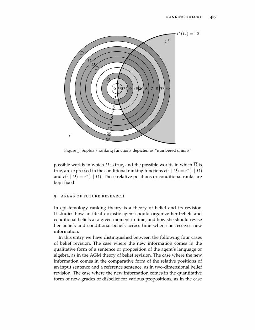
ranking theory 427
∞
∞
D
20
33
10
8
D
9
7
D
8
6
D
7
20
5
18
2
0
D
1
140 13
r∗(D) = 13
r
r∗
Figure 5: Sophia’s ranking functions depicted as “numbered onions”
possible worlds in which D is true, and the possible worlds in which D istrue, are expressed in the conditional ranking functions r(· | D) = r∗(· | D)
and r(· | D) = r∗(· | D). These relative positions or conditional ranks arekept fixed.
5 areas of future research
In epistemology ranking theory is a theory of belief and its revision.It studies how an ideal doxastic agent should organize her beliefs andconditional beliefs at a given moment in time, and how she should reviseher beliefs and conditional beliefs across time when she receives newinformation.
In this entry we have distinguished between the following four casesof belief revision. The case where the new information comes in thequalitative form of a sentence or proposition of the agent’s language oralgebra, as in the AGM theory of belief revision. The case where the newinformation comes in the comparative form of the relative positions ofan input sentence and a reference sentence, as in two-dimensional beliefrevision. The case where the new information comes in the quantitativeform of new grades of disbelief for various propositions, as in the case

428 franz huber
∞
∞
D
. . .
. . .
20
33
. . .
. . .
10
8
D
9
7
D
8
6
D
7
20
5
18
. . .
. . .
2
0
D
1
140 13
r∗(D) = 13
r
r∗
Figure 6: Sophia’s ranking functions depicted as “numbered onions” with emptylayers

ranking theory 429
of update rules 1 and 2 of ranking theory. And the case where the newinformation comes in the quantitative form of differences between theold and new grades of disbelief for such sentences or propositions, as inupdate rule 3 of ranking theory.
Let us call information that concerns only individual sentences or propo-sitions of the agent’s language or algebra factual information, and the corre-sponding changes in belief factual belief changes. In this entry we have onlydiscussed factual information and factual belief changes. Besides thesethere are at least two other forms of information an ideal doxastic agentcan receive and, corresponding to these, at least two forms of non-factualbelief change. I will briefly mention these and then I will conclude bymentioning applications of ranking theory outside epistemology, in thephilosophy of science, in metaphysics, and in the philosophy of language.
The first of these non-factual belief changes takes place when the idealdoxastic agent learns that her language or algebra was too poor or coarse-grained. For instance, Sophia may start out with a language that allows herto distinguish between red wine and white wine, and then may acquirethe concept of rosé. Or she may learn that among the red wines one candistinguish between barriques and non-barriques. When the ideal doxasticagent receives such conceptual information she should perform a conceptualbelief change. A prominent conceptual change is that of logical learning. Inthe syntactic AGM framework logical learning is normally studied interms of belief bases (Hansson, 1999). Belief bases differ from belief sets bynot being required to be closed under the logical consequence relation.Huber (2015a) shows how logical learning, and conceptual belief changesin general, can be dealt with in the semantic framework of ranking theory.
Another form of non-factual information is meta-information, and anideal doxastic agent receiving meta-information should perform a meta-belief change (Stalnaker, 2009). Information about her own doxastic state,as well as about (in-) dependencies among propositions, as reported byindicative conditionals, causal claims, and counterfactual conditionals,may be a form of meta-information. In the syntactic AGM framework onemight be able to study meta-changes with the help of dynamic doxasticlogic, DDL (Segerberg 1995; Lindström and Rabinowicz 1999; Caie, thisvolume). DDL allows one to reason about one’s own beliefs. In the semanticframework of ranking theory reasoning about one’s own beliefs has beenstudied by Spohn (2012, chaper 9) based on Hild (1998). Huber (2015a)shows how indicative conditionals can be learned in ranking theory.
In the philosophy of language Spohn (2013, 2015) uses ranking theoryto develop a unified theory of indicative, counterfactual, and many otherconditionals. On this expressivist account most conditionals express con-ditional beliefs, but counterfactuals express propositions relative to theagent’s conditional beliefs and a partition. Huber (2014b, 2017) introduces

430 franz huber
so-called alethic ranking functions and defines counterfactuals in terms ofthem. Raidl (forthcoming) proves completeness results for these and othersemantics, and corrects mistakes in Huber (2014b, 2015b, 2017). Alethicranking functions are related to subjective ranking functions by “the royalrule.” This is a normative principle that constrains a priori subjective ranksby alethic ranks much like Lewis (1980)’s principal principle constrains apriori subjective credences by objective chances. Huber (2017) show theroyal rule to be the necessary and sufficient means to attaining a cognitiveend that relates true beliefs in purely factual, non-modal propositions andtrue beliefs in purely modal propositions. The philosophical backgroundfor this is an idealism about alethic or metaphysical modality that contrastswith the projectivist account of the metaphysical modalities of chance andnecessity developed by Spohn (2010a).
In metaphysics Spohn (1983, 2006a) uses ranking theory to develop atheory of causation. This theory works with subjective ranking functions,and so results in a subjective notion of causation, although there are at-tempts at objectification (Spohn, 1993, 2012, chapter 15). Huber (2011) usesthe above-mentioned alethic ranking functions to arrive at a counterfactualnotion of causation. The conditional nature of ranking functions and aprecisification of Lewis’ (1979, p. 472) “system of weights or priorities”allow Huber (2013c) to unify the two modalities of so-called “extendedcausal models” (Halpern 2008; Halpern and Hitchcock 2010) into the onemodality of alethic ranking functions. Spohn (2010b) relates ranking theoryand causal models in a very different way.
In the philosophy of science Spohn explicates ceteris paribus conditions(Spohn, 2002, 2014) and laws (Spohn, 2005) in terms of subjective rankingfunctions. Huber (2015b) shows how the statistical notion of modes can beused to empirically confirm the above-mentioned counterfactuals that aredefined in terms of alethic ranking functions.
None of this compares to Spohn (2012), which is the most comprehen-sive treatment of ranking theory, and an invaluable resource for formalepistemology full of philosophical insights.
acknowledgments
I am very much indebted to Wolfgang Spohn. This entry would not havebeen possible without him. I think this is true—even trivially so, as hehas invented ranking theory. He thinks this is not true, at least not in anystraightforward sense (Spohn, 2015, Section 8), but merely expresses myconditional belief. Therefore let me put it in terms we understand in thesame way, except that we do not, because he understands them better thananyone else. He has taught me everything in this entry that remains after

ranking theory 431
iterated contractions by all falsehoods. I am very grateful to him for doingso.
I am also very grateful to the editors of The Open Handbook of FormalEpistemology, Richard Pettigrew and Jonathan Weisberg, for their extensiveand helpful feedback, and for putting so much time and energy intoediting this wonderful volume.
In preparing this entry I have relied on and, with permission of Wiley,reused the material from Huber (2013a, 2013b). My research was sup-ported by the Canadian SSHRC through its Insight program and by theConnaught Foundation through its New Researcher program.
references
Alchourrón, C. E., Gärdenfors, P., & Makinson, D. (1985). On the logicof theory change: Partial meet contraction and revision functions.Journal of Symbolic Logic, 50, 510–530.
Bewersdorf, B. (2013). Belief and its revision (Doctoral dissertation, KonstanzUniversity).
Boutilier, C. (1995). On the revision of probabilistic belief states. NotreDame Journal of Formal Logic, 36(1), 158–183.
Boutilier, C. (1996). Iterated revision and minimal change of conditionalbeliefs. Journal of Philosophical Logic, 25, 263–305.
Briggs, R. A. (2019). Conditionals. In R. Pettigrew & J. Weisberg (Eds.), Theopen handbook of formal epistemology. PhilPapers.
Brössel, P., Eder, A.-M., & Huber, F. (2013). Evidential support and in-strumental rationality. Philosophy and Phenomenological Research, 87,279–300.
Caie, M. (2019). Doxastic logic. In R. Pettigrew & J. Weisberg (Eds.), Theopen handbook of formal epistemology. PhilPapers.
Cantwell, J. (1997). On the logic of small changes in hypertheories. Theoria,63, 54–89.
Darwiche, A. & Pearl, J. (1997). On the logic of iterated belief revision.Artificial Intelligence, 89, 1–29.
Easwaran, K. (2011a). Bayesianism I: Introduction and arguments in favor.Philosophy Compass, 6, 312–320.
Easwaran, K. (2011b). Bayesianism II: Applications and criticisms. Philoso-phy Compass, 6, 321–332.
Easwaran, K. (2019). Conditional probabilities. In R. Pettigrew & J. Weis-berg (Eds.), The open handbook of formal epistemology. PhilPapers.
Fermé, E. (2000). Irrevocable belief revision and epistemic entrenchment.Logic Journal of the IGPL, 8, 645–652.
Fermé, E. & Rott, H. (2004). Revision by comparison. Artificial Intelligence,157, 5–47.

432 franz huber
Field, H. (1978). A note on Jeffrey Conditionalization. Philosophy of Science,45, 361–367.
Foley, R. (2009). Belief, degrees of belief, and the Lockean thesis. In F. Huber& C. Schmidt-Petri (Eds.), Degrees of belief (pp. 37–47). Dordrecht:Springer.
Gärdenfors, P. (1988). Knowledge in flux: Modeling the dynamics of epistemicstates. Cambridge, MA: MIT Press.
Gärdenfors, P. & Makinson, D. (1988). Revisions of knowledge systemsusing epistemic entrenchment. In Proceedings of the 2nd conference ontheoretical aspects of reasoning about knowledge (pp. 83–95). San Fran-cisco: Morgan Kaufmann.
Gärdenfors, P. & Rott, H. (1995). Belief revision. In D. M. Gabbay, C. J.Hogger, & J. A. Robinson (Eds.), Epistemic and temporal reasoning(pp. 35–132). Oxford: Handbook of Logic in Artificial Intelligenceand Logic Programming: Volume 4. : Clarendon Press.
Genin, K. (2019). Full & partial belief. In R. Pettigrew & J. Weisberg (Eds.),The open handbook of formal epistemology. PhilPapers.
Giang, P. H. & Shenoy, P. P. (2000). A qualitative linear utility theoryfor Spohn’s theory of epistemic beliefs. In C. Boutilier & M. Gold-szmidt (Eds.), Uncertainty in artificial intelligence 16 (pp. 220–229). SanFrancisco: Morgan Kaufmann.
Goldszmidt, M. & Pearl, J. J. (1996). Qualitative probabilities for defaultreasoning, belief revision, and causal modeling. Artificial Intelligence,84, 57–112.
Grove, A. (1988). Two modellings for theory change. Journal of PhilosophicalLogic, 17, 157–170.
Haenni, R. (2009). Non-additive degrees of belief. In F. Huber & C. Schmidt-Petri (Eds.), Degrees of belief synthese library 342. (pp. 121–159). Dor-drecht: Springer.
Hájek, A. (manuscript). Staying regular? Retrieved from http://hplms.
berkeley.edu/HajekStayingRegular.pdf
Halpern, J. Y. (2008). Defaults and normality in causal structures. In Pro-ceedings of the eleventh international conference on principles of knowledgerepresentation and reasoning (kr 2008 (pp. 198–208).
Halpern, J. Y. & Hitchcock, C. R. (2010). Actual causation and the art ofmodelling. In R. Dechter, H. Geffner, & J. Halpern (Eds.), Heuristics,probability, and causality (pp. 383–406). London: College Publications.
Hansson, S. O. (1999). A textbook of belief dynamics: Theory change anddatabase updating. Dordrecht: Kluwer.
Hansson, S. O., Fermé, E., Cantwell, J., & Falappa, M. A. (2001). Credibility-limited revision. Journal of Symbolic Logic, 66, 1581–1596.
Harper, W. L. (1976). Rational conceptual change. PSA, 1976(2), 462–494.
ranking theory 433
Hawthorne, J. (2009). The lockean thesis and the logic of belief. In F. Huber& C. Schmidt-Petri (Eds.), Degrees of belief (pp. 49–74). Dordrecht:Springer.
Herzberger, H. G. (1979). Counterfactuals and consistency. Journal of Phi-losophy, 76, 83–88.
Hild, M. (1998). Auto-epistemology and updating. Philosophical Studies, 92,321–361.
Hild, M. & Spohn, W. (2008). The measurement of ranks and the laws ofiterated contraction. Artificial Intelligence, 172, 1195–1218.
Huber, F. (manuscript). Belief and counterfactuals. a study in means-end phi-losophy. Under contract with Oxford University Press.
Huber, F. (2006). Ranking functions and rankings on languages. ArtificialIntelligence, 170, 462–471.
Huber, F. (2007). The consistency argument for ranking functions. StudiaLogica, 86, 299–329.
Huber, F. (2011). Lewis causation is a special case of Spohn causation.British Journal for the Philosophy of Science, 62, 207–210.
Huber, F. (2013a). Belief revision I: The AGM theory. Philosophy Compass,8, 604–612.
Huber, F. (2013b). Belief revision II: Ranking theory. Philosophy Compass, 8,613–621.
Huber, F. (2013c). Structural equations and beyond. The Review of SymbolicLogic, 6, 709–732.
Huber, F. (2014a). For true conditionalizers Weisberg’s Paradox is a falsealarm. Symposion, 1, 111–119.
Huber, F. (2014b). New foundations of counterfactuals. Synthese, 191, 2167–2193.
Huber, F. (2015a). How to learn concepts, consequences, and conditionals.Analytica, 1, 20–36.
Huber, F. (2015b). What should I believe about what would have been thecase? Journal of Philosophical Logic, 44, 81–110.
Huber, F. (2017). Why follow the royal rule? Synthese, 194(5), 1565–1590.Jeffrey, R. C. (1983). The logic of decision. (2nd). Chicago: University of
Chicago Press.Jin, Y. & Thielscher, M. (2007). Iterated belief revision, revised. Artificial
Intelligence, 171, 1–18.Joyce, J. M. (1998). A non-pragmatic vindication of probabilism. Philosophy
of Science, 65, 575–603.Joyce, J. M. (2009). Accuracy and coherence: Prospects for an alethic epis-
temology of partial belief. In F. Huber & C. Schmidt-Petri (Eds.),Degrees of belief (pp. 263–297). Synthese Library 342. Dordrecht:Springer.

434 franz huber
Levi, I. (1977). Subjunctives, dispositions and chances. Synthese, 34, 423–455.
Lewis, D. K. (1973). Counterfactuals. Cambridge, MA: Harvard UniversityPress.
Lewis, D. K. (1979). Counterfactual dependence and time’s arrow. Noûs,13, 455–476.
Lewis, D. K. (1980). A subjectivist’s guide to objective chance. In R. C.Jeffrey (Ed.), Studies in inductive logic and probability (pp. 263–293).Vol. II. Berkeley: University of Berkeley Press.
Lin, H. (2019). Belief revision theory. In R. Pettigrew & J. Weisberg (Eds.),The open handbook of formal epistemology. PhilPapers.
Lindström, S. & Rabinowicz, W. (1999). DDL unlimited: Dynamic doxasticlogic for introspective agents. Erkenntnis, 50, 353–385.
Nayak, A. C. (1994). Iterated belief change based on epistemic entrench-ment. Erkenntnis, 41, 353–390.
Percival, P. (2002). Epistemic consequentialism. In Proceedings of the aris-totelian society (pp. 121–151). Supplementary Volume 76.
Pettigrew, R. (2011). Epistemic utility arguments for probabilism. In E. N.Zalta (Ed.), The Stanford encyclopedia of philosophy.
Pettigrew, R. (2013). Epistemic utility and norms for credence. PhilosophyCompass, 8, 897–908.
Popper, K. R. (1955). Two autonomous axiom systems for the calculus ofprobabilities. British Journal for the Philosophy of Science, 6, 51–57.
Raidl, E. (forthcoming). Completeness for counter-doxa conditionals—using ranking semantics. The Review of Symbolic Logic. doi:10.1017/S1755020318000199
Raidl, E. (2018). Ranking semantics for doxastic necessities and condition-als. In P. Arazim & T. Lávicka (Eds.), Logica yearbook 2017. CollegePublications.
Rényi, A. (1955). On a new axiomatic system for probability. Acta Mathe-matica Academiae Scientiarum Hungaricae, 6, 285–335.
Rott, H. (2001). Change, choice, and inference: A study of belief revision andnonmonotonic reasoning. Oxford: Oxford University Press.
Rott, H. (2003). Coherence and conservatism in the dynamics of belief. PartII: Iterated belief change without dispositional coherence. Journal ofLogic and Computation, 13, 111–145.
Rott, H. (2006). Revision by comparison as a unifying framework: Severewithdrawal, irrevocable revision and irrefutable revision. TheoreticalComputer Science, 355, 228–242.
Rott, H. (2007). Two-dimensional belief change: An advertisement. In G.Bonanno, J. Delgrande, J. Lang, & H. Rott (Eds.), Formal models ofbelief change in rational agents. Dagstuhl Seminar Proceedings 07351.

ranking theory 435
Rott, H. (2009). Shifting priorities: Simple representations for twenty-seveniterated theory change operators. In D. Makinson, J. Malinowski,& H. Wansing (Eds.), Towards mathematical philosophy (pp. 269–296).Trends in Logic 28. Dordrecht: Springer.
Segerberg, K. (1995). Belief revision from the point of view of doxasticlogic. Bulletin of the IGPL, 3, 535–553.
Segerberg, K. (1998). Irrevocable belief revision in dynamic doxastic logic.Notre Dame Journal of Formal Logic, 39, 287–306.
Shenoy, P. P. (1991). On Spohn’s rule for revision of beliefs. InternationalJournal of Approximate Reasoning, 5, 149–181.
Spohn, W. (1983). Eine theorie der kausalität. Unpublished Habilitation thesis.Munich: LMU Munich, 1983.
Spohn, W. (1986). On the representation of Popper Measures. Topoi, 5,69–74.
Spohn, W. (1988). Ordinal conditional functions: A dynamic theory of epis-temic states. In W. L. Harper & B. Skyrms (Eds.), Causation in decision,belief change, and statistics II (pp. 105–134). Dordrecht: Kluwer.
Spohn, W. (1990). A general non-probabilistic theory of inductive reasoning.In R. D. Shachter, T. S. Levitt, J. Lemmer, & L. N. Kanal (Eds.),Uncertainty in artificial intelligence (pp. 149–158). Amsterdam, North-Holland.
Spohn, W. (1993). Causal laws are objectifications of inductive schemes.In J. Dubucs (Ed.), Philosophy of probability (pp. 223–252). Dordrecht:Kluwer.
Spohn, W. (1999). Ranking functions, AGM style. In S. H. B. Hansson, N.-e.Sahlin, & W. Rabinowicz (Eds.), Internet festschrift for peter gärdenfors.Lund. Retrieved from www.lucs.lu.se/spinning/categories/
dynamics/Spohn/Spohn.pdf
Spohn, W. (2002). Laws, ceteris paribus conditions, and the dynamics ofbelief. Erkenntnis, 57, 373–394.
Spohn, W. (2005). Enumerative induction and lawlikeness. Philosophy ofScience, 72, 164–187.
Spohn, W. (2006a). Causation: An alternative. British Journal for the Philoso-phy of Science, 57, 93–119.
Spohn, W. (2006b). Isaac Levi’s potentially surprising epistemologicalpicture. In E. J. Olsson (Ed.), Knowledge and inquiry: Essays on thepragmatism of Isaac Levi. New York: Cambridge University Press.
Spohn, W. (2010a). Chance and necessity: From Humean supervenienceto Humean projection. In E. Eells & J. Fetzer (Eds.), The place ofprobability in science (pp. 101–131). Boston Studies in the Philosophyof Science 284. Dordrecht: Springer.
Spohn, W. (2010b). The structural model and the ranking theoretic ap-proach to causation: A comparison. In R. Dechter, H. Geffner, &

436 franz huber
J. Halpern (Eds.), Heuristics, probability, and causality (pp. 507–522).London: College Publications.
Spohn, W. (2012). The laws of belief. ranking theory and its philosophical appli-cations. Oxford: Oxford University Press.
Spohn, W. (2013). A ranking-theoretic approach to conditionals. CognitiveScience, 37, 1074–1106.
Spohn, W. (2014). The epistemic account of ceteris paribus conditions.European Journal for the Philosophy of Science, 4, 385–408.
Spohn, W. (2015). Conditionals: A unifying ranking-theoretic perspective.Philosophers’ Imprint, 15(1), 1–30.
Stalnaker, R. C. (1970). Probability and conditionality. Philosophy of Science,37, 64–80.
Stalnaker, R. C. (2002). Epistemic consequentialism. In Proceedings of thearistotelian society supplementary volume, 76 (pp. 153–168).
Stalnaker, R. C. (2009). Iterated belief revision. Erkenntnis, 70, 189–209.Titelbaum, M. G. (2019). Precise credences. In R. Pettigrew & J. Weisberg
(Eds.), The open handbook of formal epistemology. PhilPapers.Vineberg, S. (2000). The logical status of conditionalization and its role in
confirmation. In N. Shanks & R. B. Gardner (Eds.), Logic, probabilityand science (pp. 77–94). Poznan Studies in the Philosophy of theScience: Rodopi.
Weisberg, J. (2009). Commutativity or holism? A dilemma for conditional-izers. British Journal for the Philosophy of Science, 60, 793–812.
Weisberg, J. (2011). Varieties of Bayesianism. In D. M. Gabbay, S. Hartmann,& J. Woods (Eds.), Handbook of the history of logic, volume 10, inductivelogic (pp. 477–551). Oxford: Elsevier.
Weisberg, J. (2015). Updating, undermining, and independence. BritishJournal for the Philosophy of Science, 66, 121–159.
Wenmackers, S. (2019). Infinitesimal probabilities. In R. Pettigrew & J.Weisberg (Eds.), The open handbook of formal epistemology. PhilPapers.
9F U L L & PA RT I A L B E L I E F Konstantin Genin
Philosophers and scientists in allied fields use the term ‘belief’ to referroughly to the attitude taken toward a proposition regarded as true. Thatfirst approximation is unlikely to satisfy those in search of a non-circulardefinition. Early twentieth-century psychologists and philosophers of mindattempted to address that difficulty by reducing belief to some sort ofbehavioral disposition. Although the behaviorist project is usually taken tohave been a failure, there is broad consensus that belief leaves a distinctivebehavioral footprint: most philosophers would agree that an agent whobelieves P can be expected to accept P as a premise in reasoning, planningand deliberation. If I believe that the A train is running express, I willplan to take it if going to Harlem, but try to catch the local if going tothe Museum of Natural History. Similarly banal examples can be easilymultiplied.
It is commonly held that belief is not just an all-or-nothing matter, butadmits of degrees. A veteran subway rider may have a higher degreeof belief in the proposition that the A train will run local next weekendthan in the proposition that the A train will run local next rush hour.Philosophers sufficiently impressed by examples of this sort orient theiractivity around the structure of “partial belief” rather than the all-or-nothing attitude denoted by “full belief,” or belief simpliciter. Although itis easy to generate plausible examples of partial beliefs, it is harder to sayexactly what is meant by a degree of belief. An agent’s degree of belief inP may reflect their level of confidence in the truth of P, their willingness toassent to P in conversation, or perhaps how much evidence is required toconvince them to abandon their belief in P. A venerable tradition, receivingclassical expression in Ramsey (1931) and de Finetti (1937), holds thatdegrees of belief are most directly reflected in which bets regarding P anagent is willing to accept. At least since Pascal, mainstream philosophicalopinion has held that degrees of belief are well-modeled by probabilities(see Hacking, 1975, for a readable history). To this day, subjective, or“epistemic,” probability remains one of the dominant interpretations of theprobability calculus.
A parallel tradition, though never as dominant, holds that degrees ofbelief are neither so precise, nor as definitely comparable as suggestedby Pascal’s probabilistic analysis. Keynes (1921) famously proposes thatdegrees of belief may enjoy only an ordinal structure, which admits of
437

438 konstantin genin
qualitative, but not quantitative, comparison. Keynes even suggests thatthe strength of some pairs of partial beliefs cannot be compared at all.
Cohen (1980) traces another minority tradition to Francis Bacon’s NovumOrganum. On the usual probability scale a degree of belief of zero insome proposition implies maximal conviction in its negation. On theBaconian scale, a degree of belief of zero implies no conviction in eitherthe proposition or its negation. Thus, the usual scale runs from “disproofto proof” whereas the Baconian runs from “no evidence, or non-proof toproof” (Cohen, 1980, p. 224). In the past few decades, Baconian probabilityhas received increasing attention, resulting in theories approaching thematurity and sophistication of those in the Pascalian tradition (Spohn,2012; Huber, this volume).
Formal epistemologists are traditionally interested in both full andpartial belief, although most would probably take partial belief as theprimary object of study. Moss (2018) even argues that there are instancesof probabilistic knowledge that do not involve any full beliefs. On theother hand, traditional analytic epistemologists and philosophers of mindroutinely study full belief and related all-or-nothing attitudes such asknowledge and desire, but only rarely show interest in their gradedcounterparts. The differential emphasis on partial beliefs, although oftencommented upon, may reflect sociological factors more than any essentialdifference between the fields. These differences will likely become lesspronounced in the future.
What is less often remarked upon is traditional epistemology’s focuson individual beliefs, rather than entire systems of belief, as is typicalin formal epistemology. Traditional philosophers are interested in whatit means for an agent S to believe a particular proposition P. Represen-tationalist philosopher of mind wonder how intentional states, or statesthat involve “aboutness” arise at all, especially if the agents involved arecorrectly understood as purely physical systems. Formal epistemologiststend to take matters of mental representation for granted, rarely inquiringinto how the trick is worked. Dispositionalist philosophers of mind areinterested in analyzing an agent’s belief that P into a disposition to reasonor act, although they will disagree about how readily these dispositionswill be observed in behavior. Their focus on individual beliefs gives riseto certain standard objections. A Muscovite who believes, in the 1930s,that the Stalinist terror is morally wrong, may not betray her beliefs in herbehavior at all.
Formal epistemologists resolve such difficulties by insisting on a holismabout belief: it is entire systems of belief (and perhaps utility) that arereflected in deliberation and action, otherwise underdetermined by in-dividual beliefs. In general, formal epistemologists are interested in thenorms governing the structure and dynamics of whole systems of full or

full & partial belief 439
partial belief: how individual beliefs must systematically cohere in order tobe rational; how they must be reflected in decision making; and how theyought to accommodate new evidence. Accordingly, those issues will be thefocus of this article. For a good introduction to belief in the philosophy ofmind, see Schwitzgebel (2015). See Hájek and Lin (2017) for a suggestivediscussion of how mainstream and formal epistemology would benefitfrom increased sensitivity to each other’s concerns.
Not everyone agrees that both partial and full beliefs exist—there aretheorists who attempt to eliminate one or the other attitude. But any-one who admits the existence of both full and partial belief inherits athorny problem: how are full beliefs related to partial beliefs? Two answersimmediately suggest themselves. The first claims that full belief is justthe maximal degree of partial belief. The second argues that full beliefis just partial belief above a certain threshold. Both answers give rise toformidable problems. Other theorists claim that an agent’s partial beliefsunderdetermine their full beliefs in the absence of information about theagent’s preferences.
In the last few years, the question of how partial and full belief arerelated has received considerable attention in formal epistemology, givingrise to several subtle, elegant and, unfortunately, incompatible solutions.The debate between these alternatives is the heart of this article and ispresented in Section 5. The preceding sections develop the context andbackground necessary to understand and appreciate this debate. Readerswho feel comfortable with these prerequisites, as well as those who are ina hurry, may skip to the final section and refer back to previous sectionsonly as necessary.
1 the objects of belief
In the following we will see several proposed models for the structureof belief. Most of these proposals take the objects of belief to be eitherpropositions, or sentences in a formalized language. This section reviewsthe basic notions required to work with propositions and sentences. Ifthe reader feels overwhelmed with the technicalities in this section, theyshould feel free to postpone them, and refer back to it on-the-fly. Readerswho are accustomed to working with these objects may freely skip thissection.
For our purposes, a possible world is a way the world, or some interestingaspect of the world, might be. We let W denote the set of all possibleworlds, i.e. the set of all possible ways the world might be. It is notnecessary to think of these as objective, metaphysical realities. More often,possible worlds are constrained by contextual presuppositions, and theirgranularity reflects our interests. Suffice it to say that knowing the true

440 konstantin genin
possible world w ∈ W would satisfy an agent’s curiosity—she wouldthereby settle some interesting matter under discussion. A propositionP ⊆ W is a set of possible worlds, i.e. it is a partial specification of theway the world is. To know that P is true is to know that the true world isamong the set of worlds w : w ∈ P since P is true in a possible world wiff w ∈ P.
Propositions enjoy a set-theoretic structure. The relative complementof P, ¬P = W \ P, is the set of all worlds in which P is false. If P, Qare arbitrary propositions, then their intersection P ∩ Q is the set of allworlds in which P and Q are both true. The disjunction P ∪ Q is the setof worlds in which at least one of P, Q is true. The material conditionalP→ Q is the set of worlds ¬P ∪Q, in which either P is false or Q is true.If P ⊆ Q we say that P entails Q and also that P is logically stronger thanQ. If P ⊆ Q and Q ⊆ P we write P ≡ Q and say that P and Q are logicallyequivalent. The tautological proposition W is true in all worlds and thecontradictory proposition, the empty set ∅, is not true in any world. A setof propositions A is consistent iff there is a world in which all the elementsof A are true, i.e. if ∩A 6= ∅. Otherwise, we say that A is inconsistent. Aset of propositions A is mutually exclusive iff the truth of any one elementimplies the falsehood of all other elements. The set of logical consequencesof A, written Cn(A), is the set B ⊆W : ∩A entails B. Note that if A isinconsistent, then Cn(A) is ℘(W), the set of all propositions over W.
A set of propositions F is a field (sometimes algebra) iff F contains Wand it is closed under intersection, union and complementation. That isto say that if A, B are both elements of F then W, A ∪ B, A ∩ B, and ¬Aare also elements of F . A set of propositions F is a σ-field (sometimesσ-algebra) iff it is a field that is closed under countable intersections, i.e. ifS ⊆ F is a countable collection of propositions, then the intersection ofall its elements ∩S is also an element of F . That definition implies that aσ-field is also closed under countable unions. It is not difficult to provethat an intersection of σ-fields is also a σ-field. That implies that everycollection of propositions F generates σ(F ), the least σ-field containingF , by intersecting the set of all σ-fields containing F .
Propositions, although usually expressed by sentences in a language,are not themselves sentences. That distinction is commonly drawn bysaying that propositions are semantic objects, whereas sentences are syn-tactic objects. Semantic objects (like propositions) are meaningful, sincethey represent meaningful possibilities, whereas bits of syntax must be“interpreted” before they become meaningful. In a slogan: sentences arepotentially meaningful, whereas propositions already are.
For our purposes, a language Λ is identified with the set of all grammat-ical sentences it contains. Sentences will be denoted by lowercase lettersp, q, . . .. The language Λ is assumed to contain a set of atomic sentences

full & partial belief 441
a, b, . . . which are not built out of any other sentences, as well as all the sen-tences generated by combining the atomic sentences with truth-functionalconnectives from propositional logic. In other words: if p, q are sentencesin Λ then ¬p, p∨ q, p∧ q, p→ q, and p↔ q are also sentences in Λ. Theseare meant to be read respectively as “not p,” “p or q,” “p and q,” “if p,then q,” and “p if and only if q.” The symbol ⊥ (pronounced “falsum”)denotes an arbitrarily chosen contradiction (e.g. p ∧ ¬p) and the symbol> denotes an arbitrary tautology. Some of the sentences in Λ follow “log-ically” from others. For example, under the intended interpretation ofthe truth-functional connectives, p follows from the sentence p ∧ q andalso from the set of sentences q, q → p. To capture the essentials oflogical consequence, we introduce a consequence operator, which maps anyset of sentences Γ to its logical consequences Cn(Γ). The consequenceoperator is assumed to satisfy the following properties, which abstract thecharacteristic features of deductive logic.
Γ ⊆ Cn(Γ). (Inclusion)
If Γ ⊆ ∆, then Cn(Γ) ⊆ Cn(∆). (Monotony)
Cn(Γ) = Cn(Cn(Γ)). (Idempotence)
Inclusion merely expresses the triviality that any sentence p is a deduc-tive consequence of itself. Monotony expresses the fact that adding morepremises to a deductive argument allows you to derive all the same con-clusions as you could with fewer. Idempotence says that Cn(∆) contains allthe deductive consequences of ∆. We use Γ ` p as an alternative notationfor p ∈ Cn(Γ) and Γ 0 p for p /∈ Cn(Γ). We write ` p for p ∈ Cn(∅). Theset of theorems of propositional logic is denoted by Cn(∅) since these canbe derived from the axioms alone, without any additional assumptions.
In the following, we will sometimes assume that the consequence opera-tor satisfies the following additional property:
q ∈ Cn(∆ ∪ p) implies (p→ q) ∈ Cn(∆). (Deduction theorem)
The deduction theorem expresses the fact that you can prove the condi-tional sentence p→ q by assuming p and then deriving q. Unsurprisingly,it is possible to prove that this property holds for most deductive logicsone would encounter, including both propositional and first-order logic.
There is, of course, a systematic way to map sentences in a languageto propositions. A valuation function V maps every atomic sentence a inΛ to a proposition V(a), the set of worlds in which a is true under thatinterpretation of the atoms. The valuation function also interprets thenon-atomic sentences in a way that respects the intended meanings ofthe logical connectives, i.e. so that V(>) = W, V(¬p) = W \ V(p), andV(p∧ q) = V(p)∩V(q). In this fashion, each sentence in Λ is mapped to a

442 konstantin genin
set of possible worlds. Each language Λ and valuation function V generatethe field FΛ,V = V(p) : p ∈ Λ. In turn, FΛ,V generates σ(FΛ,V), theleast σ-field containing it.
We write Γ p if for all valuations V,⋂q∈Γ
V(q) ⊆ V(p).
Then, Γ p expresses the fact that no matter how the non-logical vocabu-lary of Λ are interpreted, p is true in all the worlds in which all sentencesin Γ are true. We say that p is valid iff > p, i.e if W ⊆ V(p) for allvaluation functions. Then, p is valid iff p is true in all possible worlds, nomatter how the non-logical vocabulary are interpreted. For example, thesentence p ∨ ¬p is valid.
We assume the following property of our deductive consequence rela-tion.
If Γ ` p, then Γ p. (Soundness)
Soundness says that if the sentence p is a derivable consequence of theset of sentences Γ, then no matter how the non-logical vocabulary ofΛ are interpreted, p is true in all the worlds in which all the sentencesin Γ are true. That is to say that from true premises, our consequencerelation always derives true conclusions. Soundness also implies thatevery theorem is valid. Soundness is a basic requirement of any deductiveconsequence relation, and illustrates the intended connection betweendeductive proof and semantic entailment.
Sentences are, in a sense, capable of expressing distinctions that propo-sitions cannot. For example, the two sentences p and ¬¬p are obviouslydistinct. But if p and q are provably equivalent, i.e. if ` p ↔ q, thenp ` q and q ` p. By Soundness, p q and q p. Therefore,for any valuation function, V(p) = V(q). So p and q must express thesame proposition. Of course, an agent who is unaware of the equivalencemight believe p without believing q. What’s worse, every sentence p suchthat ` p must express the tautological proposition W. Of course, ordinaryagents do not always recognize theorems of propositional logic. For thisreason, some argue that it is sentences, rather than propositions, that arethe appropriate objects of belief. However, most of the proposed modelswe will study require that rational agents adopt the same belief attitudetoward logically equivalent sentences. So long as that is required, thereis no significant difference between taking the objects of belief to be sen-tences or propositions. Still others are not satisfied with either sentences,or propositions. Perry (1979), Lewis (1979) and Stalnaker (1981) arguethat in order to capture essentially indexical beliefs—beliefs that essentiallyinvolve indexicals such as I, here, or now—the objects of belief must be

full & partial belief 443
centered propositions. We will not take up this helpful suggestion here,but see Liao (2012) for a discussion of the costs and benefits of centeredpropositions.
2 structures for full belief
2.1 Non-monotonic Logic
In Section 1 we introduced the notion of a deductive consequence relation.The characteristic feature of a deductive consequence relation is thatconclusions are not retracted when premises are added.
If Γ ⊆ ∆, then Cn(Γ) ⊆ Cn(∆). (Monotony)
Of course, all sorts of seemingly rational everyday reasoning violatesMonotony. Reasoning according to typicality seems justified in ordinarycircumstances, but fails to satisfy Monotony. If you were told that Tweety isa bird, you would be justified in concluding that Tweety flies, since typicalbirds fly. You would retract your conclusion however, if you were to learnthat Tweety is a penguin. That does not mean that your original inferencewas unreasonable or irrational. Inductive inference is also famously non-monotonic. After observing one hundred white swans, you might concludethat all swans are white. Of course, you would retract your conclusionif you ever came across a black swan. Pace Pyrrhonian skepticism, theremust be at least some justified inductive inferences. Ethical reasoning isalso shot through with non-monotonicities. Ross (1930) discusses primafacie duties, or defeasible obligations, that are binding unless supersededby more urgent, and competing obligations. Ullman-Margalit (1983) pointsout that legal reasoning routinely relies on presumptions—of innocence,good faith, sanity, etc.—that may be withdrawn in light of new evidence.Non-Monotony is simply unavoidable in ordinary human contexts.
Non-monotonic logic studies a defeasible consequence relation |∼ be-tween premises, on the left of the wavy turnstile, and conclusions on theright. One may think of the premises on the left as a set Γ of sentencesexpressing “hard evidence” that an agent may possesses, and the conclu-sions on the right to be the defeasible conclusions that are justified on thebasis of Γ. Thus, the expression Γ |∼ p may be read as “if I were to learnall and only the sentences in Γ, I would be justified in concluding that p.”
Recall from Section 1 that a deductive consequence relation satisfiesSoundness, i.e. Γ ` p only if p is true in all the worlds in which allsentences in Γ are true. It is clear from the preceding examples thatdefeasible reasoning cannot satisfy Soundness. If Γ |∼ p then perhaps p istrue in “typical” worlds in which Γ is true, or in “most” worlds in whichΓ is true, or perhaps p is a sharply testable possibility compatible with Γ.

444 konstantin genin
We call a consequence relation ampliative if Γ |∼ p, but there are worlds inwhich all sentences in Γ are true, but p is false. It is possible to constructconsequence relations that are non-ampliative and non-monotonic, butampliativity and non-monotonicity go hand in hand in all paradigmaticcases.
The field of artificial intelligence has, since its inception, been concernedwith implementing some form of rational, ampliative, non-monotonicreasoning in artificial agents. For these purposes, deductive consequencerelations are unhelpfully restrictive. That does not preclude the possibilitythat there is some other logic that governs good ampliative reasoning. Thepast forty years have seen the creation of many logics for non-monotonicinference, often developed to model a specific kind of defeasible reasoning.See Strasser and Antonelli (2018) for an excellent overview.
In view of this profusion of specialized logics, non-monotonic logic inves-tigates which properties a logic of defeasible consequence must have inorder to count as a logic at all.1 Non-monotonic logic provides a cruciallingua franca for comparing different logics of defeasible inference. It isalso extremely apt for the purposes of this article, because it allows us tocompare different normative theories of how beliefs ought to be updatedin light of new evidence, as well as theories of how full and partial beliefsought to relate to each other.
Before we proceed to the technical development, it will be helpful tointroduce an important early critique of nonmonotonic logic due to thephilosopher John Pollock. Pollock (1987) identifies two sources of non-monotonicity in defeasible reasoning. An agent may believe p, because shebelieves q and takes q to be a defeasible reason for p. Pollock distinguishestwo kinds of defeaters for this inference: a rebutting defeater is a defeasiblereason to believe ¬p, whereas an undercutting defeater is a reason to believe¬q. Either kind of defeater may induce an agent to retract her belief in p.Pollock’s point is that since nonmonotonic logics typically do not representthe structure of an agent’s reasons, they often fail to elegantly handle casesof undercutting defeat. We shall soon see several examples.
2.1.1 Principles for Nonmonotonic Logic
Let Λ be a formal language, and let Cn(·) be a deductive consequencerelation, as discussed in Section 1. There are in fact two closely relatedapproaches to the study of non-montonic consequence relations. Thefinitary approach studies a relation between individual sentences p |∼q. That approach is taken, for example, in the very influential Kraus,Lehmann, and Magidor (1990). The infinitary approach studies a relationΓ |∼ p between an arbitrary set of sentences on the left and individual
1 Gabbay (1985) was the first to suggest this abstract point of view.

full & partial belief 445
sentences on the right. That approach is taken in the canonical referencework Makinson (1994) and cannot in general be simulated by the finitaryapproach. For the most part we will follow Makinson (1994). However,some results are known to hold only for the finitary settings. Furthermore,the more general infinitary principles are sometimes better appreciatedby their finitary consequences. For that reason, we will sometimes switchback and forth between the infinitary and the finitary approach. We writeC(Γ) for the set p : Γ |∼ p. shorthand for Γ ∪ p |∼ q.
If defeasible logics fail to satisfy Monotony, which principles ought theysatisfy? Are there some logical principles which ought to be validated byall rational defeasible reasoning? Almost all consequence relations studiedin the literature satisfy the following principle.
Γ ⊆ C(Γ). (Inclusion)
In its single-premise formulation Inclusion merely says that p |∼ p, whichis surely unexceptionable. The following two principles are also widelyaccepted in non-monotonic logic.
Γ ⊆ ∆ ⊆ C(Γ) implies C(∆) ⊆ C(Γ). (Cut)
Γ ⊆ ∆ ⊆ C(Γ) implies C(Γ) ⊆ C(∆). (Cautious Monotony)
As special cases, these two principles entail:
Γ |∼ p and Γ ∪ p |∼ q implies Γ |∼ q; (Cut)
Γ |∼ p and Γ |∼ q implies Γ ∪ p |∼ q. (Cautious Monotony)
Cut says that adding conclusions inferred from Γ to the set of premisesdoes not increase inferential power. Cautious Monotony says that it doesnot decrease inferential power. If we think of the premises on the left of|∼ as my set of “hard” evidence, and the set C(Γ) as a theory inductivelyinferred on the basis of Γ, then Cautious Monotony is an expression ofhypothetico-deductivism: if I observe a consequence of my theory C(Γ),I should not thereby retract any previous conclusions. Moreover, Cutsays that I should not add any new conclusions. Taken together the twoprinciples say that if you observe a consequence of your theory, you shouldnot change it:
Γ ⊆ ∆ ⊆ C(Γ) implies C(Γ) = C(∆). (Cumulativity)
Gabbay (1985) proposes that (finitary versions of) Inclusion, Cut andCautious Monotony are the minimal properties that every interesting non-monotonic logic must satisfy. That remains the consensus view to this day.It is easy to show that Inclusion and Cut jointly imply a principle familiarfrom Section 1:

446 konstantin genin
C(Γ) = C(C(Γ)). (Idempotence)
There is also the question of how a non-monotonic consequence relationC(·) should interact with a classical relation of deductive consequenceCn(·). The following principle says that defeasible reasoning allows youto make strictly more conclusions than classical deductive reasoning:
Cn(Γ) ⊆ C(Γ). (Supraclassicality)
That is perhaps unreasonable if we think of C(·) as modeling the defeasiblereasoning of some bounded agent. It begins to sound better if we think ofC(Γ) as modeling the ampliative conclusions that are justified on the basisof Γ.
Makinson (1994) observes that any supraclassical C(·) that satisfiesIdempotence and Cumulativity also satisfies the following pair of princi-ples.
Cn(C(Γ)) = C(Γ). (Left Absorption)
C(Γ) = C(Cn(Γ)). (Right Absorption)
Left Absorption says that C(Γ) is closed under deductive consequence.Right Absorption says that the conclusions that are justified on the basisof Γ depend only on the logical content of Γ, and not on its mode ofpresentation. The conjunction of Right and Left Absorption is called FullAbsorption.
Makinson advocates for one more interaction principle:
C(Γ) ∩ C(∆) ⊆ C(Cn(Γ) ∩ Cn(∆)). (Distribution)
That condition is perhaps too complex to admit of an intuitive gloss. How-ever, we can better understand its meaning from its finitary consequences.Any supraclassical consequence relation satisfying Distribution and FullAbsorption also satisfies the following.
Γ ∪ p |∼ r and Γ ∪ q |∼ r implies Γ ∪ p ∨ q |∼ r. (Or)
Γ ∪ p |∼ q and Γ ∪ ¬p |∼ q implies Γ |∼ q. (Case reasoning)
These two principles seem to be very compelling. Any genuine conse-quence relation ought to enable reasoning by cases. If I would infer qirrespective of what I learned about p, I should be able to infer q before thematter of p has been decided. Similarly, if p follows defeasibly from both pand q, it ought to follow from their disjunction. Any consequence relationthat satisfies Supraclassicality, Left Absorption and Case Reasoning mustalso satisfy the following principle:
Γ ∪ p |∼ q implies Γ |∼ p→ q. (Conditionalization)
full & partial belief 447
To prove that entailment suppose that Γ ∪ p |∼ q. Since p → q is adeductive consequence of q, it follows by Left Absorption that Γ ∪ p |∼p → q. Furthermore, since p → q is a deductive consequence of ¬p itfollows by supraclassicality that Γ ∪ ¬p |∼ p → q. By Case Reasoning,Γ |∼ p→ q.
Conditionalization says that upon learning new evidence, you never“jump to conclusions” that are not entailed by the deductive closure ofyour old beliefs with the new evidence. That is not an obviously appealingprinciple. An agent that starts out with Γ = Cn(∅) will either fail tovalidate Conditionalization or never make any ampliative inferences atall. Suppose that after observing 100 black ravens an agent validatingConditionalization comes to believe that all ravens are black. Then, at theoutset of inquiry, she must have believed that either all ravens are black,or she will see the first non-black raven among the first hundred. Such anagent seems strangely opinionated about when the first counterexampleto the inductive generalization must appear.
For a more realistic example, consider the 1887 Michelson-Morely ex-periment. After a null result failing to detect any significant differencebetween the speed of light in the prevailing direction of the presumedaether wind, and the speed at right angles to the wind, physicists turnedagainst the aether theory. If the physicists validated Conditionalizationthen, before the experiments, they must have believed that either there isno luminiferous aether, or the aether wind blows quickly enough to bedetected by their equipment. But why should they have been so confidentthat the aether wind is not too slow to be detectable? Even if there isnothing objectionable about an agent who validates Conditionalization,there is something very anti-inductivist about the thesis that all justifieddefeasible inferences on the basis of new evidence can be reconstructedas deductive inferences from prior conclusions plus the new evidence.Schurz (2011) makes a similar criticism, in a slightly different context:
Inductive generalizations as well as abductive conjectures ac-company belief expansions by new observations, in science aswell as in common sense cognitions. After observing severalinstances of a ‘constant conjunction,’ humans almost automat-ically form the corresponding inductive generalization; andafter performing a new experimental result sufficiently manytimes, experimental scientists proclaim the discovery of a newempirical law . . . [Conditioning]-type expansion is not at allcreative but merely additive: it simply adds the new informa-tion and forms the deductive closure, but never generates new(non-logically entailed) hypotheses.

448 konstantin genin
Schurz objects that, according to Conditionalization, dispositions to forminductive generalizations must be “programmed in” with material con-ditionals at the outset of inquiry. Anyone sympathetic to this view mustreject either Supraclassicality, Left Absorption, or Case Reasoning. Findingsuch surprising consequences of seemingly unproblematic principles isone of the boons of studying non-monotonic logic.
We finish this section by introducing one more prominent and con-troversial principles of non-monotonic logic. The position one takes onthis principle will determine how one feels about many of the theorieswhich we turn to in the following. Kraus et al. (1990) claim that any ra-tional reasoner should validate the following strengthening of CautiousMonotony.
Γ |∼ p and Γ |∼ ¬q entails Γ ∪ q |∼ p. (Rational Monotony)
Rational Monotony says that so long as new evidence q is logically compat-ible with your prior beliefs C(Γ), you should not retract any beliefs fromC(Γ). Accepting both Rational Monotony and Conditionalization amountsto saying that when confronted with new evidence that is logically con-sistent with her beliefs, a rational agent responds by simply forming thedeductive closure of her existing beliefs with the new evidence. On thatview, deductive logic is the only necessary guide to reasoning, so longas you do not run into contradiction. Stalnaker (1994) gives the followingwell-known purported counterexample to Rational Monotony.
Suppose an agent initially believes the following about the three com-posers Verdi, Bizet, and Satie.
(Iv) Verdi is Italian;
(Fb) Bizet is French;
(Fs) Satie is French.
Let p be the sentence that Verdi and Bizet are compatriots, i.e. (Fv ∧Fb) ∨ (Iv ∧ Ib). Let q be the sentence that Bizet and Satie are compatriots.Suppose that the agent receives the evidence p. As a result, she retractsher belief in Iv∧ Fb concluding that either Verdi and Bizet are both Frenchor they are both Italian. She retains her belief that Satie is French. Noticethat after updating on p, she believes it is possible that Bizet and Satie arecompatriots, i.e. p |∼ ¬q. Now suppose that she receives the evidence q.Since q is compatible with all her previous conclusions, Rational Monotonyrequires her to conclude that all three composers are French. However, itseems perfectly rational to suspend judgment and concludes that the threeare either all Italian, or all French.
Kelly and Lin (forthcoming) give the following counterexample to Ratio-nal Monotony, based on Lehrer’s (1965) no-false-lemma variant of Gettier’s

full & partial belief 449
famous (1963) scenario. There are just two people in your office, namedAlice and Bob. You are interested in whether one of them owns a certainFord. Let p be the sentence that Alice owns the Ford. Let q be the sentencethat Bob has the Ford. You have inconclusive evidence that Alice ownsthe Ford—you saw her driving one just like it. You have weaker evidencethat Bob owns the Ford—his brother owns a Ford dealership. Based onthat evidence Γ you conclude p ∨ q, i.e. that someone in the office ownsthe Ford, but do not go so far as inferring p, or q. You ask Alice and shetells you that the Ford she was driving was rented. That defeats your mainreason for p ∨ q, therefore you retract your belief that someone in the officehas a Ford. But since Γ |∼ ¬p, Rational Monotony requires you to concludethat Bob owns the Ford. However, there does not seem to be anythingirrational about how you have reasoned. This seems to be an illustrationof Pollock’s (1987) point: the logic is going wrong because it is ignoringthe structure of the agent’s reasons.
We end this section on a terminological note. It is common in theliterature to use System P (Preferential) to refer to the following set ofsingle-premise principles, labeled so that the reader can identify theirinfinitary analogues. The terminology is due to Kraus et al. (1990).
p |∼ p. (Reflexivity)
` p↔ q and p |∼ r implies q |∼ r. (Left equivalence)
` q→ r and p |∼ q implies p |∼ r. (Right weakening)
p |∼ q and p |∼ r implies p |∼ q ∧ r. (And)
p |∼ r and q |∼ r implies p ∨ q |∼ r. (Or)
p |∼ q and p |∼ r implies p ∧ q |∼ r. (Cautious monotony)
System R (Rational) arises from System P by adding a single-premiseversion of Rational Monotony:
p |∼ r and p |∼ ¬q implies p ∧ q |∼ r. (Rational monotony)
2.1.2 Preferential Semantics
So far we have considered a non-monotonic consequence relation merelyas a relation between syntactic objects. We can rephrase properties ofnon-monotonic logic “semantically,” i.e. in terms of the possible worlds inwhich the sentences are true or false. In some cases, this allows us to givea very perspicuous view on defeasible logic.
Recall from Section 1 that a deductive consequence relation satisfiesSoundness, i.e. that Γ ` p only if p is true in all the worlds in whichall sentences in Γ are true. As we have discussed, non-monotonic logics

450 konstantin genin
are ampliative, and therefore must violate Soundness. Shoham (1987)inaugurated a semantics for non-monotonic logics in which Γ |∼ p only ifp is true in a “preferred” set of worlds in which Γ is true. These are usuallyinterpreted as the “most typical,” or “most normal” worlds in which allsentences in Γ are true. If Γ is a set of sentences in Λ and V is a valuationfunction, we write V(Γ) as shorthand for ∩q∈ΓV(q). See Section 1 if youneed a refresher on valuation functions. Kraus et al. (1990) first provedmost of the results of this section for single-premise consequence relations.We follow Makinson (1994) in presenting their infinitary generalizations.
A preferential model is a triple 〈W, V,<〉 where W is a set of possibleworlds, V is a valuation function and < is an arbitrary relation on theelements of W. The relation < is transitive iff x < y and y < z impliesx < z. The relation < is irreflexive iff for all w ∈ W it is not the case thatw < w. A transitive, irreflexive relation is called a strict order. We writew ≤ v iff w < v or w = v. The strict order < is total iff for w, v ∈W eitherw ≤ v or v ≤ w.
If Γ is a set of sentences, we say that w ∈ Min<(Γ) iff w ∈ V(Γ) andthere is no v ∈ V(Γ) such that v < w. In other words, w ∈ Min<(Γ) iff wis a <-minimal element of V(Γ). Every preferential model gives rise to aconsequence relation by letting
Γ |∼< p iff Min<(Γ) ⊆ V(p),
i.e. Γ |∼< p iff p is true in all the minimal worlds in which all sentences inΓ are true. Write C<(Γ) for the set p : Γ |∼< p.
We say that a preferential model is stoppered iff for every set of sentencesΓ, if w ∈ V(Γ) then there is v ≤ w such that v ∈ Min<(Γ). (Note thatKraus et al., 1990, called stoppered models smooth models.) Makinson(1994) proves the following.
Theorem 1 Suppose that M = 〈W, V,<〉 is a preferential model. Then C<(·)satisfies Inclusion, Cut, Supraclassicality, and Distribution. If M is stoppered,then C<(·) also satisfies Cautious Monotony.
Makinson (1994) also gives the following two partial converses. The latteressentially reports a result from Kraus et al. (1990).
Theorem 2 If C(·) satisfies Inclusion, Cut, and Cautious Monotony, there is astoppered preferential model M = 〈W, V,<〉 such that C(·) = C<(·).
Theorem 3 If C(·) satisfies Inclusion, Cut, Cautious Monotony, Supraclas-sicality, and Distribution, then there is a stoppered preferential model M =
〈W, V,<〉 such that for all finite ∆ ⊆ Λ, C(∆) = C<(∆). Moreover, M may beconstructed such that < is a strict order.

full & partial belief 451
Taken together, Theorem 1 and Theorem 3 say that, at least for finitaryconsequences, the consequence relations generated by preferential modelsare exactly the consequence relations satisfying Inclusion, Cut, CautiousMonotonicity, Supraclassicality, and Distribution. In fact, one can alwaysthink of these preferential models as generated by a strict (partial) order.The question remains whether there are any natural conditions on pref-erential models that ensure that Rational Monotony is also satisfied. Itturns out that Rational Monotony follows from the requirement that thepreference relation < is a total order.
Say that a preferential model M = 〈W, V,<〉 is modular iff for allw, u, v ∈ W, if w < u ≈ v then w < v. Here u ≈ v means that u, vare unordered, i.e. it is not the case that u < v and it is not the case thatv < u. If < is a strict order, modularity is equivalent to the intuitive prop-erty of rankedness: there is a totally ordered set T and a function ρ : W → Tsuch that for all u, v ∈ W, u < v iff ρ(u) ρ(v), where is the totalordering of T. Makinson proves the following.
Theorem 4 Suppose that M = 〈W, V,<〉 is a preferential model. If M is mod-ular, then C<(·) satisfies Rational Monotony.
Kraus et al. (1990) prove the following partial converse.
Theorem 5 If C(·) finitarily satisfies Inclusion, Cut, Cautious Monotony,Supraclassicality, Distribution, and Rational Monotony, then there is a ranked,stoppered preferential model M = 〈W, V,<〉 such that for all finite ∆ ⊆ Λ,C(∆) = C<(∆). Moreover, M may be constructed such that < is a strict order.
The essential difference between preferential models that satisfy RationalMonotony and those that do not is that the former correspond to thosegenerated by a ranked partial order. This result is helpful to keep in mindbecause in the following we will see several models of belief that canbe understood as arising from a total plausibility order, and some thatarise from a merely partial plausibility order. In light of Theorem 3 andTheorem 5, we can expect the former to satisfy System R and the latter tosatisfy only the weaker System P.
2.2 AGM Belief Revision Theory
The theory of belief revision is concerned with how to update one’s beliefsin light of new evidence, especially when new evidence is inconsistentwith prior beliefs. It is especially occupied with the following sort ofscenario, borrowed from Gärdenfors (1992). Suppose that you believe allthe following sentences:
(a) All European swans are white;

452 konstantin genin
(b) The bird in the pond is a swan;
(c) The bird in the pond comes from Sweden;
(d) Sweden is in Europe.
Now suppose that you were to learn the sentence e that the bird in thepond is black. Clearly, e is inconsistent with your beliefs a, b, c, d. If youwant to incorporate the new information e and remain consistent, youwill have to retract some of your original beliefs. The problem of beliefrevision is that deductive logic alone cannot tell you which of your beliefsto give up—this has to be decided by some other means. Consideringa similar problem, Quine and Ullian (1970) enunciated the principle of“conservatism,” counseling that our new beliefs “may have to conflict withsome of our previous beliefs; but the fewer the better.” In his (1990), Quinedubs this the “maxim of minimal mutilation.” Inspired by these suggestiveprinciples, Alchourrón, Gärdenfors, and Makinson (1985) develop a highlyinfluential theory of belief revision, known thereafter as AGM theory, afterits three originators.
In AGM theory, beliefs held by an agent are represented by a set Bof sentences. The set B is called the belief state of the agent. This set isusually assumed to be closed under logical consequence. Of course, thisis an unrealistic idealization, since it means that the agent believes alllogical consequences of her beliefs. Levi (1991) defends this idealizationby changing the interpretation of the set B—these are the sentences thatthe agent is committed to believe, not those that she actually believes.Although we may never live up to our commitments, Levi argues that weare committed to the logical consequences of our beliefs. That may rescuethe principle, but only by changing the interpretation of the theory.
AGM theory studies three different types of belief change. Contractionoccurs when the belief state B is replaced by B ÷ p, a logically closedsubset of B no longer containing p. Expansion occurs when the belief stateB is replaced with B + p = Cn(B ∪ p), the result of simply adding p tothe set of beliefs and closing under logical consequence. Revision occurswhen the belief state B is replaced by B ∗ p, the result of adding p to B andremoving whatever is necessary to ensure that the resulting belief stateB ∗ p is logically consistent.
Contraction is the fundamental form of belief change studied by AGM.There is no mystery in how to define expansion, and revision is usuallydefined derivatively via the Levi identity (1977): B ∗ p = (B ÷ ¬p) + p.Alchourrón et al. (1985) and Gärdenfors and Makinson (1988) proceedaxiomatically: they postulate several principles that every rational con-traction operation must satisfy. Fundamental to AGM theory are severalrepresentation theorems showing that certain intuitive constructions give

full & partial belief 453
rise to contraction operations satisfying the basic postulates and conversely,that every operation satisfying the basic postulates can be seen as the out-come of such a construction. See Lin (this volume) for an introduction tothese results.
AGM theory is unique in focusing on belief contraction. For someoneconcerned with maintaining a database, contraction is a fairly naturaloperation. Medical researchers might want to publish a data set, but makesure that it cannot be used to identify their patients. Privacy regulationsmay force data collectors to “forget” certain facts about you and, naturally,they would want to do this as conservatively as possible. However, aplausible argument holds that all forms of rational belief change occurring“in the wild” involve learning new information, rather than conservativelyremoving an old belief. All the other formalisms covered in the articlefocus on this form of belief change. For this reason, we focus on the AGMtheory of revision and neglect contraction.
Before delving into some of the technical development, we mentionsome important objections and alternatives to the AGM framework. Aswe have mentioned, the belief state of an agent is represented by the(deductively closed) set B of sentences the agent is committed to believe.The structure of the agent’s reasons is not represented: you cannot tell ofany two p, q ∈ B whether one is a reason for the other. Gärdenfors (1992)distinguishes between foundations theories, that keep track of which beliefsjustify which others, and coherence theories, which ignore the structure ofjustification and focus instead on whether beliefs are consistent with oneanother. Arguing for the coherence approach, Gärdenfors (1992) draws astark distinction between the two:
According to the foundations theory, belief revision shouldconsist, first, in giving up all beliefs that no longer have a satis-factory justification and, second, in adding new beliefs that havebecome justified. On the other hand, according to the coherencetheory, the objectives are, first, to maintain consistency in therevised epistemic state, and, second, to make minimal changesof the old state that guarantee overall coherence.
Implicit in this passage is the idea that foundations theory are fundamen-tally out of sympathy with the principle of minimal mutilation. Elsewhere(1988), Gärdenfors is more apologetic, suggesting that some hybrid theoryis possible and perhaps even preferable:
I admit that the postulates for contractions and revisions thathave been introduced here are quite simpleminded, but theyseem to capture what can be formulated for the meager struc-ture of belief sets. In richer models of epistemic states, admit-ting, for example, reasons to be formulated, the corresponding

454 konstantin genin
conservativity postulates must be formulated much more cau-tiously (p. 67).
Previously, we have seen Pollock (1987) advocating for foundationalism. Inartificial intelligence, Doyle’s (1979) reason maintenance system is taken toexemplify the foundations approach. Horty (2012) argues that default logicaptly represents the structure of reasons. For a defense of foundationalism,as well as a useful comparison of the two approaches, see Doyle (1992).
Another dissenting tradition advocates for belief bases instead of beliefstates. A belief base is a set of sentences that is typically not closedunder logical consequence. Its elements represent “basic” beliefs that arenot derived from other beliefs. This allows us to distinguish betweensentences that are explicit beliefs, like “Shakespeare wrote Hamlet” andnever thought-of consequences like “Either Shakespeare wrote Hamlet orAlan Turing was born on a Monday.” Revision and contraction are thenredefined to operate on belief bases, rather than belief sets. That allows forincreased expressive power, since belief bases which have the same logicalclosure are not treated interchangeably. For an introduction to belief basessee Hansson (2017). For a book-length treatment, see Hansson (1999).
Finally, one of the most common criticisms of AGM theory is that it doesnot illuminate iterated belief change. In the following, we shall see that thecanonical revision operation takes as input an entrenchment ordering on abelief state, but outputs a belief state without an entrenchment order. Thatseverely underdetermines the result of a subsequent revision. For more onthe problem of iterated belief revision, see Huber (2013a).
The treatment in this article is necessarily rather compressed. There areseveral excellent survey articles on belief revision. See Hansson (2017),Huber (2013a, 2013b), and Lin (this volume).
2.2.1 Revision
Alchourrón et al. (1985) propose the following postulates for rational beliefrevision.
B ∗ p = Cn(B ∗ p). (Closure)
p ∈ B ∗ p. (Success)
B ∗ p ⊆ Cn(B ∪ p). (Inclusion)
If ¬p /∈ Cn(B), then B ⊆ B ∗ p. (Preservation)
B ∗ p is consistent if p is consistent. (Consistency)
If (p↔ q) ∈ Cn(∅), then B ∗ p = B ∗ q. (Extensionality)

full & partial belief 455
By now, Closure, Success, Consistency, and Extensionality should bestraightforward to interpret. These postulates impose synchronic con-straints on B ∗ p. Preservation and Inclusion are the only norms that arereally about revision—they capture the diachronic spirit of AGM revision.Inclusion says that revision by p should yield no more new beliefs thanexpansion by p. In other words, any sentence q that you come to believeafter revising by p is a deductive consequence of p and your prior beliefs.Consider the following principle:
If q ∈ B ∗ p, then (p→ q) ∈ B. (Conditionalization)
In Section 2.1.1, we considered an analogue of Conditionalization fornonmonotonic logic. All the same objections apply equally well in thecontext of belief revision. Recall from Section 1 that a deductive conse-quence relation admits a deduction theorem iff ∆ ∪ p ` q implies that∆ ` p → q. So long as a deduction theorem is provable for Cn(·), Inclu-sion and Conditionalization are equivalent. To see this, suppose that therevision operation ∗ satisfies Inclusion. Then, if q ∈ B ∗ p, it follows thatB ∪ p ` q. By the deduction theorem, B ` p → q. For the converse,suppose that the revision operation ∗ satisfies Conditionalization. Then,if q ∈ B ∗ p, it follows that p→ q ∈ B and q ∈ Cn(B ∪ p). If you foundany of the arguments against Conditionalization convincing, you ought tobe skeptical of Inclusion.
Preservation says that, so long as the new information p is logically con-sistent with your prior beliefs, all of your prior beliefs survive revision byp. In the setting of non-monotonic logic, we called this principle RationalMonotony. All objections and counterexamples to Rational Monotony fromSection 2.1.1 apply equally well in belief revision. As we have seen, Preser-vation rules out any kind of undercutting defeat of previously successfuldefeasible inferences. Accepting both Preservation (Rational Monotonicity)and Inclusion (Conditionalization) amounts to saying that when con-fronted with new evidence that is logically consistent with her beliefs, arational agent responds by simply forming the deductive closure of herexisting beliefs with the new evidence. On that view, deductive logic isthe only necessary guide to reasoning, so long as you do not run intocontradiction.
Alchourrón et al. (1985) also propose the following supplementaryrevision postulates, closely related to Inclusion and Preservation.
B ∗ (p ∧ q) ⊆ (B ∗ p) + q. (Conjunctive Inclusion)
If ¬q /∈ Cn(B ∗ p),then (B ∗ p) + q ⊆ B ∗ (p ∧ q). (Conjunctive Preservation)

456 konstantin genin
It is possible to make the connection between belief revision and nonmono-tonic logic precise. Given a belief set B and a revision operation ∗, we candefine a single-premise consequence relation by setting
p |∼ q iff q ∈ B ∗ p.
Similarly, given a single-premise consequence relation |∼ we can define
B = p : > |∼ p and B ∗ p = q : p |∼ q.
Then it is possible to prove the following correspondences between AGMbelief revision and the set of single-premise principles we called System Rin Section 2.1.1. It follows, by Theorem 5, that AGM revision can be repre-sented in terms of a ranked, stoppered preferential model over possibleworlds.
Theorem 6 Suppose that ∗ is a revision operation for B satisfying all eightrevision postulates. Then, the nonmonotonic consequence relation given by p |∼ qiff q ∈ B ∗ p satisfies all the principles of System R.
Theorem 7 Suppose that |∼ is a consequence relation that satisfies all the prin-ciples of System R and such that p |∼ ⊥ only if ` ¬p. Then, the revisionoperation ∗ defined by letting B = p : > |∼ p and B ∗ p = q : p |∼ qsatisfies all eight revision postulates.
2.2.2 Entrenchment
Gärdenfors and Makinson (1988) introduce the notion of an entrenchmentrelation on sentences.
Even if all sentences in a [. . . ] set are accepted or consideredas facts [. . . ], this does not mean that all sentences are of equalvalue for planning or problem-solving purposes. Certain [. . . ]beliefs about the world are more important than others whenplanning future actions, conducting scientific investigations,or reasoning in general. We will say that some sentences [. . . ]have a higher degree of epistemic entrenchment than others. Thedegree of entrenchment will, intuitively, have a bearing on whatis abandoned [. . . ], and what is retained, when a contractionor revision is carried out.
To model the degree of entrenchment, Gärdenfors and Makinson (1988)introduce a relation ≤ holding between sentences of the language Λ. Thenotation p ≤ q is pronounced “p is at most as entrenched as q.” Gärdenforsand Makinson (1988) propose that the entrenchment relation ≤ satisfy thefollowing postulates.

full & partial belief 457
If p ≤ q and q ≤ r, then p ≤ r. (Transitivity)
If p ` q, then p ≤ q. (Dominance)
Either p ≤ (p ∧ q), or q ≤ (p ∧ q). (Conjunctiveness)
If B is consistent, then p /∈ B iff p ≤ q for all q. (Minimality)
If q ≤ p for all q, then p ∈ Cn(∅). (Maximality)
Note that, in light of Minimality, an entrenchment relation is defined fora particular belief set B. It follows from the first three of these postulatesthat an entrenchment order is total, i.e. for all p, q either p ≤ q or q ≤ p.
Given a belief set B and an entrenchment relation ≤, it is possible todefine a revision operation directly by setting:
B ∗ p = Cn(q ∈ Λ : ¬p < q ∪ p). (C∗)
The idea behind this equation is that the agent revises by p by first clearingfrom her belief set anything less entrenched than ¬p, (by dominance, thisincludes everything entailing ¬p) adding p, and then closing under logicalconsequence. This illustrates why AGM theory is not a theory of iteratedrevision: the revision operation takes as input an entrenchment order andbelief state, but outputs only a belief state. That severely underdeterminesthe results of subsequent revisions. Gärdenfors (1988) proves the following.
Theorem 8 If a relation ≤ satisfies the five entrenchment postulates, then therevision function ∗ determined via (C∗) satisfies the six basic and the two sup-plementary revision postulates.
Finally, given a belief set B, an entrenchment relation can be recoveredfrom a revision operation by setting:
p ≤ q iff p /∈ B ∗ ¬(p ∧ q) or ` q. (C∗≤)
The idea is that p is no more entrenched than q if p does not survive arevision by ¬(p ∧ q) or if q is a tautology. Rott (2003) proves the following.
Theorem 9 If a revision operation ∗ satisfies the six basic and the two supple-mentary contraction postulates, then the entrenchment relation determined via(C∗≤) satisfies the five entrenchment postulates.
2.2.3 Sphere Semantics
So far we have thought of belief revision syntactically: a revision operation∗ takes in a set B of syntactic objects and a sentence p and outputs anotherset of sentences B ∗ p. Grove (1988) gives a perspicuous way to represent

458 konstantin genin
the revision postulates semantically, i.e. in terms of the possible worlds inwhich the sentences are true or false.
As before, let W be a set of possible worlds and let V : Λ→ ℘(W) bea valuation function.2 If Γ is a set of sentences in Λ, we write V(Γ) asshorthand for ∩q∈ΓV(q). If E is a proposition, we write T(E) as shorthandfor p ∈ Λ : E ⊆ V(p), i.e. the set of all sentences p such that E entailsV(p).
A set of propositions S is a system of spheres centered on V(B) ⊆ W ifffor all E, F ⊆W and all p ∈ Λ, the following conditions hold.
If E, F ∈ S , then E ⊆ F or F ⊆ E. (Nested)
V(B) ∈ S and if E ∈ S then V(B) ⊆ E. (Centered)
W ∈ S . (Maximum)
If p 0 ⊥, then there is E ∈ S such thatE ∩V(p) 6= ∅ and if F ∩V(p) 6= ∅ then E ⊆ F. (Well order)
In other words, a system of spheres centered on V(B) is a nested setof propositions, all entailed by V(B), with the following property: if pis a consistent sentence, then there is a logically strongest element ofS consistent with V(p). If p is a consistent sentence, let S(p) be E ∩V(p), where E is the logically strongest element of S consistent withV(p). Otherwise, let S(p) = ∅. In other words: S(p) is the set of worldscompatible with V(p) that is “closest” to V(B) according to the spheresystem. Note that if V(p) ∩ V(B) 6= ∅, then S(p) = V(B) ∩ V(p). IfV(p) ∩ V(B) = ∅ we find the closest sphere compatible with V(p) andintersect the two. Given a belief set B and a system of spheres S centeredon V(B) we can define a revision operator by setting:
B ∗ p = T(S(p)).
The idea is this: when you revise on a sentence p compatible with yourprevious beliefs, then the strongest proposition you believe is V(p)∩V(B).If p is incompatible with your beliefs, you fall back to E ∩ V(p), whereE is the p-compatible proposition closest to your old belief V(B). Thus,the system of spheres S can be seen as a set of “fallback positions” forupdating on incompatible propositions. See Figure 1.
Grove (1988) proves the following.
Theorem 10 Let B be a belief set. For each system of spheres S centered onV(B), there is an operation ∗ satisfying the six basic and the two supplementaryrevision postulates such that B ∗ p = T(S(p)). Moreover, for every revision op-eration ∗ satisfying the six basic and the two supplementary revision postulates,there is a sphere system S centered on V(B) such that B ∗ p = T(S(p)).
2 See Section 1 if you need a refresher on valuation functions.

full & partial belief 459
V(B)
V(p)
V(B ∗ p)
Figure 1: A system of spheres centered on V(B). The shaded region is V(B ∗ p).
Finally, the sphere semantics gives a dramatic illustration of the critiquethat AGM does not illuminate iterated belief change. A revision maps aset of spheres S and a sentence p to a set of sentences T(S(p)). It does notoutput a new set of spheres centered on the new belief state. That severelyunderdetermines the result of future revisions.
2.3 The Paradox of the Preface
The models of full belief that we have seen so far require that beliefs beconsistent and closed under deductive consequence. While it is admittedthat this requirement is not psychologically realistic, or perhaps evenfeasible for bounded agents, it is proffered as a normative principle thatwe should strive to approximate. After all, consistency and closure arenecessary conditions for achieving the following two related ends: believingonly true sentences (consistency) and believing as many true sentences aspossible without risking error in any more possible worlds (closure).
Nevertheless, the Paradox of the Preface, due to Makinson (1965), chal-lenges even the normativity of deductive consistency. The story goes likethis. A famous theorist has just finished her latest book. As is custom-ary for such works, she includes a passage in the preface thanking hercolleagues and students for their help in editing and proofreading, butaccepting sole responsibility for the mistakes that inevitably remain. Sheseems to be saying that, despite her best efforts, she believes that noteverything that she asserts in the book is true. Let s1, . . . , sn be the claimsshe asserts in the book. Presumably, she believes each of the si or else shewould not have asserted them. Yet in the preface she claims to believe¬(s1 ∧ . . . ∧ sn), the claim that at least one of the si is false. The theorist

460 konstantin genin
seems to be behaving perfectly rationally, yet on this reconstruction thereis no way that she can be both consistent and deductively closed.
It is tempting to say that inconsistency in the service of intellectualhumility is no sin. Yet this creates a further difficulty: surely some inconsis-tencies are vicious and should be eliminated. Others, it seems, are virtuousand ought to be tolerated. But how do we know which inconsistenciesare which? If we point out an inconsistency in someone’s beliefs, we tendto think that they are under some pressure to resolve it. But why can’teveryone respond to such a challenge by claiming that their inconsistencyis a virtue? The Preface Paradox seems to challenge the very normativityof logical consistency.
There are several ways to respond to this challenge. The first, andperhaps the most common route, is to claim that belief is fundamentally amatter of degree. The theorist merely has a high degree of belief in each ofthe statements of her book. And there is nothing surprising about havinga high degree of belief in each of the si but not in their conjunction. In fact,if the structure of partial belief is probabilistic, this would emerge as asimple consequence of the probability calculus: it is to be expected that theprobability of each of the si exceeds the probability of their conjunction,so long as the probability of the si falls short of unity. This analysis alsoentails something about the relationship between full and partial belief: itis rationally admissible to fully believe statements that have a high, but notmaximal, degree of belief. These themes will be taken up in subsequentsections.
A second set of responses to the paradox calls our attention to the varietyof cognitive attitudes that are involved in the story. For example, Cohen(1992) attributes many confusions and apparent paradoxes to the erroneousconflation of two related cognitive attitudes: belief and acceptance. Beliefin p, according to Cohen, is a disposition to feel it true that p, wheneverattending to issues raised by the proposition that p. This disposition mayor may not be reflected in speech and action, and is not under directvolitional control. But to accept that p is to adopt a policy of deeming,positing, or postulating that p—i.e. of including it among one’s premisesfor deciding what to do or think in a particular context, whether or notone feels it to be true. Acceptance is a volitional matter, and is sensitive toour cognitive context.
Belief is sometimes not even a prima facie reason for acceptance: in scien-tific contexts many of our most cherished beliefs are not accepted, as it isour duty to subject them to criticism and not argue from them as premises.Cohen claims that a person who accepts nothing that she believes is intel-lectually paralyzed, but someone who accepts everything she believes isrecklessly uncritical. Furthermore, acceptance may sometimes promote be-

full & partial belief 461
lief, at least in the long run, but often has no effect: for example, a defenselawyer may accept that her client is innocent, but believe otherwise.
Cohen claims that acceptance ought to be closed, at least under ac-cepted deductive consequences. Consistency is also, presumably, a normof acceptance. Belief, however, is different:
you are not intellectually pledged by a set of beliefs, howeverstrong, to each deductive consequence of that set of beliefs,even if you recognize it to be such. That is because belief thatp is a disposition to feel that p, and feelings that arise in you[. . . ] through involuntary processes [. . . ] no more impose theirlogical consequences on you than do the electoral campaignposters that people stick on your walls without your consent.(Cohen, 1992, p. 31)
Armed with the distinction between belief and acceptance, we canattempt a redescription of the preface paradox. In the context of hertheoretical work, the theorist accepts s1, . . . , sn and is bound to maintainconsistency and accept their (accepted) deductive consequences. In fact, shewould be in dereliction of her duty as theorist if she accepted the prefacesentence in the body of the book. However, the context of the preface isdifferent: here it is customary to drop the professional exigencies of thetheorist and acknowledge broader features of the author’s cognitive life.She has fulfilled her duty as theorist and done the utmost to accept onlythose claims that are justified by her evidence and arguments. However,some of these conclusions may not yet be attended with the inner glowof belief. Perhaps, if the work meets with no devastating objections, shemay eventually cease to believe the humble claim in the preface. Thusthe distinction between belief and acceptance explains why we are notalarmed by the sentence in the context of the preface, but we would beshocked if we saw it used as a premise in the body of the text. For a similarresolution of the paradox, see Chapter 5 of Stalnaker (1984).
It is easy to underestimate the consequences of accepting Cohen’s argu-ments. For one, we would have to reinterpret all of the theories of rationalbelief that we have discussed as theories of rational acceptance. In fact,there may be no theory of rational belief, but only psychological tricksand heuristics for coming to believe, similar to those Pascal recommendsfor arriving at faith in Christ. Longstanding dogmas about the relationbetween belief and knowledge would have to be revisited. Moreover, exces-sive appeal to the distinction threatens the unity and cohesiveness of ourcognitive lives. For a discussion of these kinds of objections see Kvanvig(2016). For an overview of the distinction between belief and acceptance,see Weirich (2004).

462 konstantin genin
3 structures for partial belief
3.1 Bayesianism
Bayesianism, or subjective probability theory, is by far the dominantparadigm for modeling partial belief. The literature on the subject is bynow very large and includes many approachable introductions. The sum-mary provided here will, of necessity, be rather brief. For an article-lengthintroduction see Huber (2016), Easwaran (2011a, 2011b), or Weisberg (2011).For a book-length introduction see Earman (1992) or Howson and Urbach(2006). For an article-length introduction to Bayesian models of rationalaction, see Briggs (2017) or Thoma (this volume). For an approachablebook-length introduction to the theory of rational choice see Resnik (1987).
The heart of the Bayesian theory is roughly the following:
1. There is a fundamental psychological attitude called degree of belief(sometimes called confidence or credence) that can be represented bynumbers in the [0, 1] interval.
2. The degrees of belief of rational agents satisfy the axioms of proba-bility theory.
3. The degrees of belief of rational agents are updated by some flavor ofprobabilistic conditioning.
The first two principles are the synchronic requirements of Bayesian theory;the third principle concerns diachronic updating behavior. Most Bayesianswould also agree to some version of the following principles, which linksubjective probabilities with deliberation and action:
4. Possible states of the world (sometimes outcomes) are assigned autility: a positive or negative real number that reflects the desirabilityor undesirability of that outcome.
5. Rational agents perform only those actions that maximize expectedutility, which is calculated by weighing the utility of outcomes bytheir subjective probability.
What makes Bayesianism so formidable is that, in addition to providingan account of rational belief and its updating, it also provides an accountof rational action and deliberation. No other theory can claim a developed,fine-grained account of all three of these aspects of belief. In the followingwe will briefly spell out some of the technical details of the Bayesianpicture.

full & partial belief 463
3.1.1 Probabilism
In this section we flesh out the details of the synchronic component of theBayesian theory. For the purposes of this section we will take propositionsto be the objects of (partial) belief. It is also possible to take a syntacticapproach and assign degrees of belief to sentences in a formal language.For the most part, nothing hinges on which approach we choose. Forarguments in favor of the syntactic approach, see Weisberg (2011).
As usual, let W be a set of possible worlds. Let F be a σ-field over W.3
A credence function p assigns a degree of belief to every proposition inF . Probabilism requires that the credence function satisfies the axioms ofprobability. For every E, F ∈ F :
p(E) is a positive, real number; (Positivity)
p(W) = 1; (Unitarity)
if E ∩ F = ∅, then p(E ∪ F) = p(E) + p(F). (Additivity)
From these principles it is possible to derive several illuminating theorems.For example, the degree of belief assigned to the contradictory propositionis equal to zero. Furthermore, if E entails F, then p(E) ≤ p(F). Finally, forany proposition E ∈ F we have that 0 ≤ p(E) ≤ 1.
In the standard axiomatization of probability theory due to Kolmogorov(1950), additivity is strengthened to Countable Additivity.
If E1, E2, . . . are mutually exclusive,then p(
⋃∞i=1 Ei) = ∑∞
i=1 p(Ei). (Countable Additivity)
This requirement is not as innocent as it looks: it rules out the possibilitythat any agent is indifferent over a countably infinite set of mutuallyexclusive possibilities. De Finetti (1970, 1972) famously argued that weought to reject countable additivity since it is conceivable that God couldpick out a natural number “at random” and with equal (zero) probability.For another example, suppose you assign 50% credence to the proposition¬B that not all ravens that will ever be observed are black. Let ¬Bi bethe proposition that the ith observed raven is the first non-black ravento appear. Then ¬B =
⋃∞i=1 ¬Bi. Countable additivity entails that for all
ε > 0 there is a finite n such that p(⋃n
i=1 ¬Bi) = 1/2− ε. So you must benearly certain that if all ravens are not black, the first non-black raven willappear among the first n ravens. The only way to assign equal probabilityto all ¬Bi is to violate countable additivity by setting p(¬Bi) = 0 for all i.This solution has its own drawbacks. On all standard models of Bayesianupdate it will be impossible to become convinced that the ith raven is
3 Refer to Section 1 if you need to refresh yourself on the definition of a σ-field.

464 konstantin genin
indeed non-black, even if you are looking at a white one. For more oncountable additivity, see Chapter 13 in Kelly (1996).
Now that we have defined probabilism, it is natural to ask how to justifyit: why should a rational agent’s degrees of belief obey the probabilityaxioms? There are roughly two kinds of answers to this question currentin the Bayesian canon.
The traditional answer is that an agent that violates the axioms ofprobability opens herself up to systems of bets that, although fair from theagent’s perspective, guarantee a sure loss. Answers of this flavor are calledDutch book arguments and they require positing some connection betweendegrees of belief and fair betting quotients. Some epistemologists findDutch book arguments to be unconvincing either because they disavow anytight connection between degrees of belief and betting quotients, or theydeny that any facts about something so pragmatic as betting could havenormative epistemic force. These epistemologists tend to prefer accuracyarguments, which purport to show that any agent violating the probabilityaxioms will have beliefs which are less accurate, or “further from the truth,”than agents that satisfy the axioms. We will briefly review the traditionalDutch book-style arguments. For the original articulation of the accuracyperspective see Joyce (1998). For an article-length overview of accuracy-style arguments see Pettigrew (2016b). For a book-length treatment seePettigrew (2016a).
Dutch book arguments require specifying some connection betweendegrees of belief and fair betting quotients. For de Finetti (1937) theconnection was definitional: an agent’s degree of belief in a propositionA simply is her fair odds ratio for a bet that pays $1 if A is true andnothing otherwise. If you are willing to pay at most $.50 for a bet thatpays $1 if A is true and nothing otherwise, then it must be that yourdegree of confidence in A is 50%. It is easy to see what is wrong with thiskind of definition: there may be factors other than the subject’s degree ofbelief which affect her fair betting quotient. She may be risk averse, orrisk-loving; she may abhor gambling, or love showing off. Ramsey (1931)avoids some of these problems by pricing bets in utility, rather than money,and appealing to the existence of an “ethically neutral” proposition that isconsidered equally likely to be true and false. For more on the connectionbetween degrees of belief and betting ratios see Eriksson and Hájek (2007).
Supposing that a suitable connection between degrees of belief and fairbetting quotients exists, it is possible to construct a “Dutch book” againstan agent violating the axioms of probability. To get such an argumentgoing we suppose that if the agent’s degree of belief in A is p(A), thenshe considers fair a bet that costs $p(A) ·Y and pays $Y if A is true and$0 otherwise. Note that we allow Y to take positive and negative values.This means that the agent is willing to assume the role of the bookie and

full & partial belief 465
sell a bet that “costs” −$p(A) · Y and “pays” −$Y if A is true and $0otherwise. Now suppose that such an agent violates finite additivity. Oneway this may happen is if for A, B such that A ∩ B = ∅, we have thatp(A ∪ B) > p(A) + p(B). Then, the agent considers fair
1. a bet that costs −$p(A) and pays −$1 if A is true and $0 otherwise;
2. a bet that costs −$p(B) and pays −$1 if B is true and $0 otherwise;
3. a bet that costs $p(A ∪ B) and pays $1 if A ∪ B is true and $0otherwise.
There are three possible scenarios: either A and B are both false or exactlyone of them is true. The reader should confirm that in any of thesescenarios the agent is left with exactly $p(A) + $p(B)− $p(A∪ B) < 0. Byreversing which bets the agent buys and sells, we can construct a Dutchbook against an agent that violates additivity by having p(A∪ B) < p(A)+
p(B). Similar strategies work to construct Dutch books against agents thatviolate Positivity, Unitarity, and Countable Additivity. Furthermore, it ispossible to show that if your degrees of belief validate the probabilityaxioms, then no Dutch book can be made against you (Kemeny, 1955). Formore on Dutch book arguments see Section 3.3 in Hájek (2012).
3.1.2 Updating by Conditioning
We have discussed the synchronic content of the Bayesian theory, but westill need to talk about how degrees of belief are updated upon receivingnew information. There are two standard models of partial belief update:strict conditionalization and Jeffrey conditionalization. Strict condition-alization assumes that the information received acquires the maximaldegree of belief. Jeffrey conditionalization allows for the situation in whichno proposition is upgraded to full certainty when new information isacquired.
For all propositions A, B ∈ F such that p(A) > 0, the conditionalprobability of B given A is defined as:
p(B | A) :=p(A ∩ B)
p(A).
Conditionalization by A restricts all possibilities to those compatible withA and then renormalizes by the probability of A to ensure that unitarityholds. By far the most standard modeling of partial belief update holdsthat degrees of belief ought to be updated by conditionalization. In otherwords, if pt is your credence function at time t and A is a propositionexpressing the total new information acquired by t′ > t, then pt′ ought toequal pt(· | A), whenever pt(A) > 0.

466 konstantin genin
What if new information does not render any proposition certain, butmerely changes the subjective probability of some propositions? Jeffrey(1983) proposes the following update rule. Suppose that pt is your credencefunction at time t. Suppose that the total evidence that comes in by timet′ updates your degrees of belief in partition Ai1≤i≤n (and in no finerpartition) setting each respectively to ai with ∑i ai = 1. Then your newcredence function pt′ ought to be ∑i p(· | Ai)ai.
Why should a rational agent update by strict or Jeffrey conditionaliza-tion? Dutch-book style arguments for strict conditionalization are given inTeller (1973) and Lewis (1999) and extended to Jeffrey conditionalizationin Armendt (1980). For more see Skyrms (2009). For an accuracy-styleargument in favor of strict conditionalization and against Jeffrey condi-tionalization, see Leitgeb and Pettigrew (2010).
For our purposes it is important to point out that conditional probabilityis always a lower bound for the probability of the material conditional. Inother words, for all E, H ∈ F ,
p(H | E) ≤ p(E→ H),
whenever p(E) > 0. We can see this as a quantitative version of thequalitative principle of Conditionalization we discussed in Section 2.1.1:however confident a Bayesian agent becomes in H after updating on E,she must have been at least as confident that H is a material consequenceof E. Popper and Miller (1983) took this observation to be “completelydevastating to the inductive interpretation of the calculus of probability.”For the history of the Popper-Miller debate see Chapter 4 in Earman (1992).A similar property can be demonstrated for Jeffrey conditioning (Genin,2017).
Both strict and Jeffrey conditionalization are defined in terms of con-ditional probability. The probability of B conditional on A is standardlydefined as the ratio of the unconditional probabilities p(A ∩ B) and p(A).Clearly, this ratio is undefined when p(A) = 0. Some theorists wouldlike conditional probability to be defined even when conditioning onpropositions of probability zero. The standard approach in mathematicalstatistics, due to Kolmogorov (1950), is via the conditional expectation. Onthat approach, conditional probability remains dependent on uncondi-tional probability. An alternative approach, adopted by Popper (1955) andRenyi (1955), takes conditional probability as a primitive, rather than aderivative, notion. For a defense of the conditional expectation, see Gyenis,Hofer-Szabó, and Rédei (2017). For an introduction to primitive conditionalprobabilities, see Easwaran (this volume). For a critique of the standardnotion of conditional probability, see Hájek (2003).

full & partial belief 467
States
Good Rotten
Acts Outcomes
Break into Bowl 6-Egg Omelet No Omelet
+10 0
Break into Saucer 6-Egg Omelet, 5-Egg Omelet,
extra washing extra washing
+8 +4
Table 1: A payoff table for the morning chef
3.1.3 Deliberation and Action
One of the signal advantages of the Bayesian model of partial belief is thatit is ready-made to plug into a prominent model of practical deliberation.Decision theory, or rational choice theory, is too large and sprawling asubject to be effectively covered here, although it will be presented incursory outline. For an excellent introduction, see Briggs (2017) or Thoma(this volume). For our purposes, it is enough to note that a well-developedtheory exists and that no comparable theory exists for alternative modelsof belief.4
Suppose you would like to make a six egg omelet. You’ve broken 5 fresheggs into a mixing bowl. Rooting around your fridge, you find a looseegg of uncertain provenance. If you are feeling lucky you can break thesuspect egg directly into the mixing bowl; if you are wary of the egg, youmight break it into a saucer first and incur more dishwashing.
There are four essential ingredients to this sort of decision-theoretic sit-uation. There are outcomes, over which we have defined utilities measuringthe desirability of the outcome. In the case of the omelet the outcomes area ruined omelet or a 5–6 egg omelet, with or without extra washing. Thereare states—usually unknown to and out of the control of the actor—whichinfluence the outcome of the decision. In our case the states are exhaustedby the possible states of the suspect egg: either good or rotten. Finally,there are acts which are under the control of the decision maker. In our casethe acts include breaking the egg into the bowl or the saucer. Of coursethere are other conceivable acts: you might throw the suspect egg awayand make do with a 5-egg omelet; you might even flip a coin to decidewhat to do. We omit these for the sake of simplicity. These four elementsare usually summarized in a payoff table (see Table 1). To fit this into the
4 However, recent work such as Lin (2013) and Spohn (2017, 2019) may remedy that inade-quacy in the case of qualitative belief.

468 konstantin genin
framework of partial belief we assume that the set of acts A1, A2, . . . , An
partition W. We also assume the set of states S1, S2, . . . , Sm partition W. Weassume that the credence function assigns a probability to every outcome.We assume that acts and states are logically independent, so that no staterules out the performance of any act. Finally, we assume that given a stateof the world Sj and an act Ai there is exactly one outcome Oij, which isassigned a utility U(Oij). The ultimate counsel of rational choice theory isthat agents ought to perform only those acts that maximize expected utility.The expected utility of an act is defined as:
EU(Ai) =m
∑j=1
pAi(Sj)U(Oij),
where pAi(Sj) is roughly how likely the agent considers Sj given thatshe has performed act Ai. Difficulties about how this quantity should bedefined give rise to the schism between evidential and causal decisiontheory (see Section 3.3 in Thoma, this volume). However, in many sit-uations, including the dilemma of the omelet, the act chosen does notaffect the probabilities with which states obtain. This is called “act-stateindependence” in the jargon of rational choice theory. In cases of act-stateindependence there is broad consensus that pAi(Sj) should be equal to theunconditional degree of belief p(Sj).
Central to the literature on decision theory are a number of representationtheorems showing that every agent with qualitative preferences satisfyinga set of rationality postulates can be represented as an expected utilitymaximizer (von Neumann & Morgenstern, 1944; Savage, 1954). Theseaxioms are controversial, and are subject to intuitive counterexamples.Allais (1953) and Ellsberg (1961) give examples in which seemingly rationalagents violate the rationality postulates and therefore cannot, even inprinciple, be represented as expected utility maximizers. For more on thissubject, see Sections 2 and 3 in Briggs (2017).
3.1.4 Modifications and Alternatives
Dissatisfaction with various aspects of the Bayesian theory has spawneda number of formal projects. Many epistemologists reject the notion thatrational agents must have precise credences in every proposition that theycan entertain; instead they claim that rational agents may have imprecisecredences representable by intervals of real numbers. For an introduction toimprecise probability, see Mahtani (this volume). The theory of Dempster-Shafer belief functions (Dempster, 1968; Shafer, 1976) rejects the tightconnection between degrees of belief and fair betting ratios. Fair bettingratios ought indeed satisfy the axioms of probability, but degrees of beliefneed not. Nevertheless, it should be possible to calculate fair betting ratios

full & partial belief 469
from degrees of belief when these are necessary. For this purpose, degreesof belief may satisfy a weaker set of axioms than those of the probabilitycalculus. For an introduction to Dempster-Shafer belief functions seeSection 3.1 in Huber (2016).
Many epistemologists have held that degrees of belief are not so defi-nitely comparable as suggested by the probabilistic analysis. Keynes (1921)famously proposes that degrees of belief may enjoy only an ordinal struc-ture, which admits of qualitative, but not quantitative, comparison. Keyneseven suggests that the strength of some pairs of partial beliefs cannot becompared at all. Koopman (1940) and Fine (1973) pursue Keynes’ sugges-tions, developing axiomatic theories of qualitative probability. See Konek(this volume) for an introduction to qualitative probability comparisons.
3.2 Ranking Theory
Cohen (1977, 1980) distinguishes between two rival probabilistic traditions.Pascalian probability finds its latest expression in contemporary Bayesian-ism. But Cohen traces a rival tradition back to Francis Bacon. Roughly,these two can be distinguished by the scale they select for the strength ofbelief. On the Pascalian scale a degree of belief of zero in some propositionimplies maximal conviction in its negation. On the Baconian scale, a de-gree of belief of zero implies no conviction in either the proposition or itsnegation. Thus, the Pascalian scale runs from “disproof to proof” whereasthe Baconian runs from “no evidence, or non-proof to proof” (Cohen,1980, p. 224). Cohen (1977) argues that despite the conspicuous successesof Pascalian probability, the Baconian scale is more appropriate in othersettings, including legal proceedings.
Ranking theory, first developed in Spohn (1988), is a sophisticated contem-porary theory of Baconian probability. For an article-length introductionto ranking theory see Huber (2013; this volume). For an extensive book-length treatment, with applications to many subjects in epistemology andphilosophy of science, see Spohn (2012). We mention some of its basicfeatures, as it provides a useful counterpoint to the models of belief wehave already discussed.
As before, let W be a set of possible worlds. Let F be an algebra overW.5 A function β : F →N∪ ∞ from F into the set of natural numbersN extended by ∞, is a positive ranking function on F just in case for anyA, B ∈ F :
β(∅) = 0; (Consistency)
β(W) = ∞; (Infinitivity)
5 Refer to Section 1 if you need to refresh yourself on the definition of an algebra

470 konstantin genin
β(A ∩ B) = minβ(A), β(B). (Minimitivity)
A positive ranking function expresses degrees of belief. If β(A) > 0, thenwe may say that A is (fully) believed and ¬A is disbelieved. If β(A) = 0then A is not believed and ¬A may not be believed either. Thus, rankingtheory can be seen as satisfying the “Lockean thesis,” the intuitive proposalthat a degree of belief above some threshold is necessary and sufficient forfull belief (see Section 5.2). Note however that nothing in ranking theoryrequires us to say that the threshold is exactly zero: we could have chosenany positive number n.
Let β be a positive ranking function and A ∈ F with β(¬A) < ∞. Thenfor any B ∈ F the conditional positive rank of B given A is defined as
β(B | A) = β(¬A ∪ B)− β(¬A).
The function βA : B 7→ β(B | A) is called the conditionalization of β by Aand is itself a positive ranking function. This definition is used to articulatean update rule for ranking theory: if β is your positive ranking function attime t and between t and t′ you become certain of E ∈ F and no logicallystronger proposition, then βE should be your new ranking function attime t′. Spohn (1988) also defines ranking-theoretic analogues of Jeffreyconditioning.
It is clear from the definition of conditioning that, as in the Bayesian case,the rank of the material conditional is a lower bound for the conditionalrank: β(A→ B) ≤ β(B |A). It also satisfies a version of Rational Monotony:if β(¬A) = 0 and β(B) > 0, then β(B | A) > 0.6 Therefore, ranking-theoretic update satisfies the “spirit” of AGM update. Note however, thatranking theory has no trouble with iterated belief revision: a revision takesas input a ranking function and an evidential proposition and outputs anew ranking function.
Ranking theory lies somewhat awkwardly between a theory of full andpartial belief. On the one hand, all propositions of positive rank are fullybelieved. On the other hand, the rank of a proposition measures somethingabout the strength of that belief. But how should we interpret these ranks?Huber (this volume) investigates the relation between ranking-theoreticdegrees of belief, and AGM-style degrees of entrenchment. The degree ofentrenchment for a proposition A is defined as the number of independentand reliable information sources testifying against A that it requires for theagent to give up full belief in A. Degrees of entrenchment may be used tomeasure ranking-theoretic degrees of belief; alternatively, it is possible toidentify ranking-theoretic degrees of belief with degrees of entrenchment.Huber (manuscript) proves that if an agent defines her full beliefs from
6 Rational Monotony is not satisfied if we set the the threshold for full belief at some numbergreater than zero (Raidl, forthcoming, footnote 26).

full & partial belief 471
an entrenchment function, her beliefs will be consistent and deductivelyclosed iff the entrenchment function is a ranking function.
One of the advantages of ranking theory over AGM is that it allowsreasons to be defined (Spohn, 2012). Say that A is a reason for B with respectto the positive ranking function β iff β(B | A) > β(B | ¬A). Say that anagent has A as a reason for B iff A is a reason for B according to herpositive ranking function β and β(A) > 0. Note that it is not possible tomake such a definition in the AGM theory since the conditional degree ofentrenchment is not defined. Thus ranking theory may provide an answerto Pollock’s criticism of belief revision by allowing various kinds of defeatof reasons to be represented (Spohn, 2012, Section 11.5).
4 eliminationisms
There are those who deny that there are any interesting principles bridgingfull and partial belief. Theorists of this persuasion often want either toeliminate one of these attitudes or reduce it to a special case of the other.Jeffrey (1970) suggests that talk of full belief is vestigial and will be entirelysuperseded by talk of partial belief and utility:
. . . nor am I disturbed by the fact that our ordinary notion ofbelief is only vestigially present in the notion of degree of belief.I am inclined to think Ramsey sucked the marrow out of theordinary notion, and used it to nourish a more adequate view.But maybe there is more there, of value. I hope so. Show me; Ihave not seen it at all clearly, but it may be there for all that (p.172).
Theorists such as Kaplan (1996) also suggests that talk of full belief issuperfluous once the mechanisms of Bayesian decision theory are in place.After all, only partial beliefs (or confidence in Kaplan’s terminology) andutilities play any role in the Bayesian framework of rational deliberation,whereas full belief need not be mentioned at all. Those committed to fullbeliefs have the burden of showing what difference they make to our lives:
Making the case that talk of investing confidence leaves outsomething important—something we have in mind when wetalk of belief—is going to require honest toil. One has to say. . . exactly how an account of rational human activity will bethe poorer if it has no recourse to talk of belief. In short, onehas to meet the Bayesian Challenge. (p. 100)
Stalnaker (1984) is much more sympathetic to a qualitative notion of belief(or acceptance) but acknowledges the force of the Bayesian Challenge.

472 konstantin genin
Bayesian decision theory gives a complete account of how prob-ability values . . . ought to guide behavior . . . So what could bethe point of selecting an interval near the top of the probabilityscale and conferring on the propositions whose probability fallsin that interval the honorific title “accepted”? Unless accep-tance . . . makes a difference to how the agent behaves, or oughtto behave it is difficult to see how the concept of acceptancecan have the interest and importance for inquiry that it seemsto have. (p. 91)
It is true that there is no canonical qualitative analogue to the Bayesiantheory of practical deliberation. However, the fact that it is the theorist offull belief that feels the challenge, and not vice versa, may be an accident ofhistory: if a qualitative theory of practical deliberation had been developedfirst, the shoe would now be on the other foot. The situation wouldbe even more severe if qualitative decision making, which we seem toimplement as a matter of course, were less cognitively demanding than itsBayesian counterpart. Of course, this anticipates a robust theory of rationalqualitative deliberation that is not immediately forthcoming. However,recent work such as Lin (2013) and Spohn (2017, 2019) may remedy thatinadequacy. For example, Lin (2013) proves a Savage-style representationtheorem characterizing the relationship between full beliefs, desires overpossible outcomes, and preferences over acts. By developing a theory ofrational action in terms of qualitative belief, Lin demonstrates how onemight answer the Bayesian challenge.
On the other hand there are partisans of full belief that are deeplyskeptical about partial beliefs.7 Many of these object that partial beliefshave no psychological reality and would be too difficult to reason with ifthey did. Horgan (2017) goes so far as to say that typically “there is nosuch psychological state as the agent’s credence in p” and that Bayesianepistemology is “like alchemy and phlogiston theory: it is not about anyreal phenomena, and thus it also is not about any genuine norms thatgovern real phenomena” (p. 7). Harman (1986) argues that we have veryfew explicit partial beliefs. A theory of reasoning, according to Harman,can concern only explicit attitudes, since these are the only ones that canfigure in a reasoning process. Therefore, Bayesian epistemology, whileperhaps an account of dispositions to act, is not a guide to reasoning.Nevertheless, partial beliefs may be implicit in our system of full beliefs inthat they can be reconstructed from our dispositions to revise them.
How should we account for the varying strengths of explicit be-liefs? I am inclined to suppose that these varying strengths are
7 See Harman (1986), Pollock (2006), Moon (2017), and Horgan (2017). See also the “badcop” in Hájek and Lin (2017).

full & partial belief 473
implicit in a system of beliefs one accepts in a yes/no fashion.My guess is that they are to be explained as a kind of epiphe-nomenon resulting from the operation of rules of revision. Forexample, it may be that P is believed more strongly than Q if itwould be harder to stop believing P than to stop believing Q,perhaps because it would require more of a revision of one’sview. . . (Harman, 1986, p. 22)
On this picture, almost all of our explicit beliefs are qualitative. Partialbeliefs are not graded belief attitudes toward propositions, but rather dis-positions to revise our full beliefs. The correct theory of partial belief,according to Harman, has more to do with entrenchment orders (seeSection 2.2.2) or ranking-theoretic degrees of belief (see Section 3.2) thanwith probabilities. Other apparently partial belief attitudes are explainedas full beliefs about objective probabilities. So, in the case of a fair lotterywith ten thousand tickets, the agent does not believe to a high degree thatthe nth ticket will not win, but rather fully believes that it is objectivelyimprobable that it will win.
Frankish (2009) objects that Harman’s view requires that an agent havea full belief in any proposition that we have a degree of belief in: “Andthis is surely wrong. I have some degree of confidence (less than 50%) inthe proposition that it will rain tomorrow, but I do not believe flat-outthat it will rain—not, at least, by the everyday standards for flat-out belief”(p. 4). Harman might reply that Frankish merely has a full belief in theobjective probability of rain tomorrow. Frankish claims that this escaperoute is closed to Harman because single events “do not have objectiveprobabilities,” but this matter is hardly settled.
Staffel (2013) gives an example in which a proposition with a higherdegree of belief is apparently less entrenched than one with a lower degreeof belief. Suppose that you will draw a sequence of two million marblesfrom a big jar full of red and black marbles. You do not know whatproportion of the marbles are red. Consider the following cases.
Scenario 1. You have drawn twenty marbles, 19 black and one red. Yourdegree of belief that the last marble you will draw is black is .95.
Scenario 2. You have drawn a million marbles, 900, 000 of which havebeen black. Your degree of belief that the last marble you will drawis black is 19/20 = .90.
Staffel argues that your degree of belief in the first case is higher thanin the second, but much more entrenched in the second than in the first.Therefore, degree of belief cannot be reduced to degree of entrenchment.Nevertheless, the same gambit is open to Harman in the case of themarbles—he can claim that in both scenarios you merely have a full belief

474 konstantin genin
in a proposition about objective chance. See Staffel (2013) for a much moreextensive engagement with Harman (1986).
5 bridge principles for full and partial belief
Anyone who allows for the existence of both full and partial belief inheritsa thorny problem: how are full beliefs related to partial beliefs? That seem-ingly innocent question leads to a treacherous search for bridge principlesconnecting a rational agent’s partial beliefs with her full beliefs. Theo-rists engaged in the search for bridge principles usually take for grantedsome set of rationality principles governing full belief and its revisione.g. AGM theory, or a rival system of non-monotonic reasoning. Theoristsusually also take for granted that partial belief ought to be representableby probability functions obeying some flavor of Bayesian rationality. Thechallenge is to propose additional rationality postulates governing how arational agent’s partial beliefs cohere with her full beliefs. In this section,we will for the most part accept received wisdom and assume that ortho-dox Bayesianism is the correct model of partial belief and its updating.We will be more open-minded about the modeling of full belief and itsrational revision.
In this section, we will once again take propositions to be the objects ofbelief. In the background, there will be a (usually finite) set W of possibleworlds. As before, the reader is invited to think of W as a set of coarse-grained, mutually exclusive, possible ways the actual world might be.The actual world is assumed to instantiate one of these coarse-grainedpossibilities. We write B to denote the set of propositions that the agentbelieves and use B(A) as shorthand for A ∈ B. We will also require somenotation for qualitative propositional belief change. For all E ⊆W, writeBE for the set of propositions the agent would believe upon learning Eand no stronger proposition. We will also write B(A | E) as shorthand forA ∈ BE. By convention, B = BW . If F is a set of propositions, we let BFbe the set BE : E ∈ F. The set BF represents an agent’s dispositions toupdate her qualitative beliefs given information from F .
The following normative constraint on the set of full beliefs B plays alarge role in what follows.
For all propositions A, B ⊆W: (Deductive Cogency)
1. B(W);
2. not B(∅);3. if B(A) and A ⊆ B, then B(B);
4. if B(A) and B(B) then B(A ∩ B).

full & partial belief 475
The first two clauses say that the agent believes the true world to be amongthe worlds in W and that she does not believe the empty set to contain thetrue world. The third clause says that belief is closed under single-premiseentailment, i.e. if the agent believes A and A logically entails B, then shebelieves B. The final clause says that the agent’s beliefs are closed underconjunction, i.e. if she believes A and she believes B, then she believesA ∩ B. Together, clauses 3 and 4 say that the agent’s beliefs are closedunder entailment by finitely many premises. When W is finite, the set Bmust be finite as well, implying that Deductive Cogency is equivalent tothe following formulation:
B is consistent and B(B) iff ∩B ⊆ B. (Deductive Cogency)
In other words, Deductive Cogency means that there is a single, non-empty proposition, which is the logically strongest proposition that theagent believes, entailing all her other beliefs. When the two formulationsof Deductive Cogency come apart, we will always mean the latter one.Deductive Cogency only mentions the set of full beliefs B, and is thereforenot a bridge principle at all. Bridge principles are expressed as constraintsholding for pairs 〈B, p〉.
All of the rationality norms that we have seen for updating qualitativebeliefs have propositional analogues. The following are propositionalanalogues for the six basic AGM principles. Here E, F are arbitrary subsetsof W.
BE = Cn(BE). (Closure)
E ∈ BE. (Success)
BE ⊆ Cn(B ∪ E). (Inclusion)
If ¬E /∈ Cn(B) then B ⊆ BE. (Preservation)
BE is consistent if E 6= ∅. (Consistency)
If E ≡ F, then BE = BF. (Extensionality)
BE∩F ⊆ Cn(BE ∪ F). (Conjunctive inclusion)
If ¬F /∈ Cn(BE), thenCn(BE ∪ F) ⊆ BE∩F. (Conjunctive preservation)
Supposing that for all E ⊆W, BE satisfies Deductive Cogency, the first sixpostulates reduce to the following three, for arbitrary E ⊆W.
∩BE ⊆ E. (Success)
∩B ∩ E ⊆ ∩BE. (Inclusion)

476 konstantin genin
If ∩B * ¬E, then ∩BE ⊆ ∩B ∩ E. (Preservation)
Together, Inclusion and Preservation say that whenever information E isconsistent with current belief ∩B,
∩BE = ∩B ∩ E.
If F is a collection of propositions and for all E ∈ F , the belief sets B,BE
satisfy the AGM principles, we say that BF , the agent’s disposition toupdate her qualitative beliefs given information from F , satisfies the basicAGM principles.
We will use p(·) to denote the probability function representing theagent’s partial beliefs. Of course, p(·) is defined on a σ-algebra of subsetsof W. In the usual case, when W is finite, we can take the ℘(W) to bethe relevant σ-algebra. To update partial belief, we adopt the standardprobabilistic modeling. For E ⊆ W such that p(E) > 0, p(· | E) is thepartial belief function resulting from learning E. We will sometimes usepE as a shorthand for p(· | E). Almost always, partial belief is updated viaconditioning:
p(A | E) = p(A ∩ E)p(E)
, whenever p(E) > 0.
Let F+p be the set of propositions with positive probability according to p,
i.e A ⊆W : p(A) > 0.
5.1 Belief as Extremal Probability
The first bridge principle that suggests itself is that full belief is just themaximum degree of partial belief. Expressed probabilistically, it says thatat all times a rational agent’s beliefs and partial beliefs can be representedby a pair 〈B, p〉 satisfying:
B(A) iff p(A) = 1. (Extremal Probability)
Roorda (1995) calls this the received view of how full and partial beliefought to interact. Gärdenfors (1986) is a representative of this view, as arevan Fraassen (1995) and Arló-Costa (1999), although the latter two accepta slightly non-standard probabilistic modeling for partial belief. For fansof Deductive Cogency, the following observations ought to count in favorof the received view.
Theorem 11 If 〈B, p〉 satisfy extremal probability, then B is deductively cogent.
Gärdenfors (1986) proves the following.

full & partial belief 477
Theorem 12 Suppose that 〈BE, pE〉 satisfy extremal probability for all E ∈ F+p .
Then BF+p
satisfies the AGM postulates.
In other words: if an agent’s partial beliefs validate the probability axioms,she updates by Bayesian conditioning and fully believes all and only thosepropositions with extremal probability, her qualitative update behavior willsatisfy all the AGM postulates (at least whenever Bayesian conditioningis defined). Readers who take the AGM revision postulates to be a sinequa non of rational belief update will take this to be good news for thereceived view.
Roorda (1995) makes three criticisms of the received view. Consider thefollowing three propositions.
1. Millard Fillmore was the 13th President of the United States;
2. Millard Fillmore was a U.S. President;
3. Millard Fillmore either was or was not a U.S. President.
Of course, I am not as confident that Fillmore was the 13th president as Iam in the truth of the tautology expressed in (3). Yet there does not seemto be anything wrong with saying that I fully believe each of (1), (2), and(3). However, if extremal probability is right, it is irrational to fully believeeach of (1), (2), and (3) and not assign them all the same degree of belief.
Roorda’s second objection appeals to the standard connection betweendegrees of belief and practical decision making. Suppose I fully believe (1).According to the standard interpretation of degrees of belief in terms ofbetting quotients, I ought to be accept a bet that pays out a dollar if (1) istrue, and costs me a million dollars if (1) is false. In fact, if I truly assignunit probability to (1), I ought to accept nearly any stakes whatsoever thatguarantee some positive payout if (1) is true. Yet it seems perfectly rationalto fully believe (1) and refrain from accepting such a bet. If we acceptBayesian decision theory, extremal probability seems to commit me to allsorts of weird and seemingly irrational betting behavior.
Roorda’s final challenge to extremal probability appeals to corrigibility,according to which it is reasonable to believe that at least some of mybeliefs may need to be abandoned in light of new information. However, ifpartial beliefs are updated via Bayesian conditioning, I can never cease tobelieve any of my full beliefs since if p(A) = 1 it follows that p(A | E) = 1for all E such that p(E) > 0. If we believe in Bayesian conditioning,extremal probability seems to entail that I cannot revise any of my fullbeliefs in light of new information.

478 konstantin genin
5.2 The Lockean Threshold
The natural response to the difficulties with the received view is to retreatfrom full certainty. Perhaps full belief corresponds to partial belief abovesome threshold falling short of certainty. Foley (1993) dubbed this viewthe Lockean thesis, after some apparently similar remarks in Book IV ofLocke’s Essay Concerning Human Understanding. So far, the Lockean thesisis actually ambiguous. There may be a single threshold that is rationallymandated for all agents and in all circumstances. Alternatively, each agentmay have her own threshold that she applies in all circumstances—thatthreshold may characterize how “bold” or “risk-seeking” the agent isin forming qualitative beliefs. A yet weaker thesis holds that the thresh-old may be contextually determined. We distinguish the strong, context-independent Lockean thesis (SLT) from the weaker, context-dependentthesis (WLT). The domain of the quantifier may be taken as the set of allbelief states 〈B, p〉 a particular agent may find herself in, or as the set of allbelief states whatsoever.
Strong Lockean Thesis (SLT). There is a threshold 12 < s < 1 such that
all rational 〈B, p〉 satisfy
B(A) iff p(A) ≥ s.
Weak Lockean Thesis (WLT). For every rational 〈B, p〉 there is a thresh-old 1
2 < s < 1 such that
B(A) iff p(A) ≥ s.
Most discussions of the Lockean thesis have in mind the strong thesis.More recent work, especially Leitgeb (2017), adopts the weaker thesis. Thestrong thesis leaves the correct threshold unspecified. Of course for every12 < s < 1, we can formulate a specific thesis SLTs in virtue of which thestrong thesis is true. For example, SLT.51 is a very permissive version ofthe thesis, whereas SLT.95 and SLT.99 are more stringent. It is also possibleto further specify the weak thesis. For example, Leitgeb (2017) believes thatthe contextually-determined threshold should be equal to the degree ofbelief assigned to the strongest proposition that is fully believed. In lightof Deductive Cogency, that corresponds to the orthographically ungainlyWLTp(∩B).
The strong Lockean thesis gives rise to the well-known Lottery paradox,due originally to Kyburg (1961, 1997). The lesson of the Lottery is that thestrong thesis is in tension with Deductive Cogency. Suppose that s is theuniversally correct Lockean threshold. Now think of a fair lottery withN tickets, where N is chosen large enough that 1− (1/N) ≥ s. Since the

full & partial belief 479
lottery is fair, it seems permissible to fully believe that some ticket is thewinner. It also seems reasonable to assign degree of belief 1/N to eachproposition of the form “The ith ticket is the winner.” According to theLockean thesis, such an agent ought to fully believe that the first ticket isa loser, the second ticket is a loser, the third is a loser, etc. Since cogencyrequires belief to be closed under conjunction, she ought to believe that allthe tickets are losers. But now she violates cogency by believing both thatevery ticket is a loser and that some ticket is a winner. Since s was arbitrary,we have shown that no matter how high we set the threshold, there issome Lottery for which an agent must either violate the Lockean thesisor violate Deductive Cogency. According to Kyburg, what the paradoxteaches is that we should give up on Deductive Cogency: full belief shouldnot necessarily be closed under conjunction. Many others take the lessonof the Lottery to be that the strong Lockean thesis is untenable.
Several authors attempt to revise the strong Lockean thesis by placingrestrictions on when a high degree of belief warrants full belief. Broadlyspeaking, they propose that a high degree of belief is sufficient to warrantfull belief unless some defeating condition holds. For example, Pollock(1995) proposes that, although a degree of belief in P above some thresholdis a prima facie reason for belief, that reason is defeated whenever P isa member of an inconsistent set of propositions each of which is alsobelieved to a degree exceeding the threshold. Ryan (1996) proposes that ahigh degree of belief is sufficient for full belief unless the proposition is amember of a set of propositions such that each member has a degree ofbelief exceeding the threshold, but the probability of their conjunction isbelow the threshold. Douven (2002) says that it is sufficient except whenthe proposition is a member of a probabilistically self-undermining set. A setS is probabilistically self undermining iff for all A ∈ S , p(A) > s andp(A | B) ≤ s, where B =
⋂(S \ A). It is clear that any of these proposals
would prohibit full belief that a particular lottery ticket will lose.These proposals are all vitiated by the following sort of example due
to Korb (1992). Let A be any proposition with a degree of belief abovethreshold but short of certainty. Let Li be the proposition that the ith
lottery ticket (of a large lottery with N tickets) will lose. Consider theset S = ¬A ∪ Li | 1 ≤ i ≤ N. Each member of S is above threshold,since Li is above threshold. Furthermore, the set S ∪ A meets all threedefeating conditions. Therefore, these proposals prohibit full belief in anyproposition with degree of belief short of certainty. Douven and Williamson(2006) generalize this sort of example to trivialize an entire class of similarformal proposals.
Buchak (2014) argues that what partial beliefs count as full beliefs cannotmerely be a matter of the degree of partial belief, but must also dependon the type of evidence it is based on. According to Buchak, this means

480 konstantin genin
there can be no merely formal answer to the question: what conditionson partial belief are necessary and sufficient for full belief? The followingexample, of a type going back to Thomson (1986), illustrates the point.Your parked car was hit by a bus in the middle of the night. The bus couldbelong either to the blue bus company or the red bus company. Considerthe following two scenarios.
Scenario 1. You know that the blue company operates 90% of the busesin the area, and the red bus company operates only 10%. You havedegree of belief 0.9 that a blue bus is to blame.
Scenario 2. The red and blue companies operate an equal number ofbuses. A 90% reliable eyewitness testifies that a blue bus hit your car.You have degree of belief 0.9 that a blue bus is to blame.
Buchak (2014) argues that it is rational to have full belief that a blue busis to blame in the second scenario, but not in the first. You have onlystatistical evidence in the first scenario, whereas in the second, a causalchain of events connects your belief to the accident (see also Thomson, 1986,Nelkin, 2000, and Schauer, 2003). These intuitions, Buchak observes, arereflected in our legal practice: purely statistical evidence is not sufficientto convict. If you find Buchak’s point convincing, you will be unsatisfiedwith most of the proposed accounts for how full and partial belief oughtto correspond (Staffel, 2016).
Despite difficulties with buses and lotteries, the dynamics of qualitativebelief under the strong thesis are independently interesting to investigate.For example, van Eijck and Renne (2014) axiomatize the logic of belief fora Lockean with threshold 1
2 . Makinson and Hawthorne (2015) investigatewhich principles of non-monotonic logic are validated by Lockean agents.Before turning to proposed solutions to the Lottery paradox, we makesome observations about qualitative Lockean revision, inspired largely byShear and Fitelson (2018).
It is a theorem of the probability calculus that p(H | E) ≤ P(E→ H). Soif H is assigned a high degree of belief given E, the material conditionalE → H must have been assigned a degree of belief at least as high exante. It is easy to see that as a probabilistic analogue of the principle ofConditionalization from non-monotonic logic or, equivalently, the AGMInclusion principle. That observation has the following consequence: anybelief that the Lockean comes to have after conditioning, she could havearrived at by adding the evidence to her prior beliefs and closing underlogical consequence. Therefore Lockean updating satisfies the AGM prin-ciple of Inclusion. Furthermore, it follows immediately from definitionsthat Lockean update satisfies Success and Extensionality.

full & partial belief 481
Theorem 13 Suppose that s ∈ ( 12 , 1). Let BE = A : p(A | E) ≥ s for all
E ∈ F+p . Then BF+
psatisfies Inclusion, Success, and Extensionality.
In Section 2.2.1, we argued that Inclusion and Preservation capture thespirit of AGM revision. If Lockean revision also satisfied Preservation, wewould have a clean sweep of the AGM principles, with the exception ofDeductive Cogency.
However, that cannot hold in general. It is possible to construct exampleswhere p(¬E) < s, p(H) ≥ s, and yet p(H | E) < s. For Lockean agentsthis means that it is possible to lose a belief, even when revising on aproposition that is not disbelieved.
Recall the example of Alice, Bob, and the Ford from Section 2.1.1. LetW = a, b, c corresponding to the worlds in which Alice owns the Ford,Bob owns the Ford, and no one in the office owns the Ford. Suppose theprobability function
p(a) =610
,
p(b) =310
,
p(c) =110
,
captures my partial beliefs. For Lockean thresholds in the interval (.75, .9],my full beliefs are exhausted by B = a, b, W. Now suppose I were tolearn that Alice does not own the Ford. That is consistent with all beliefsin B, but since p(a, b | b, c) = 3
4 , it follows by the Lockean thesis thata, b /∈ Bb,c. So Lockeanism does not in general validate Preservation.The good news, at least for those sympathetic to Pollock’s critique ofnon-monotonic logic, is that the Lockean thesis allows for undercuttingdefeat of previous beliefs.
However, Shear and Fitelson (2018) also have some good news for fansof AGM and the Lockean thesis. Two quantities are in the golden ratioφ if their ratio is the same as the ratio of their sum to the larger of thetwo quantities, i.e. for a > b > 0, if a+b
a = ab then a
b = φ. The goldenratio is an irrational number approximately equal to 1.618. Its inverse φ−1
is approximately .618. Shear and Fitelson prove the following intriguingresult.
Theorem 14 Suppose that s ∈ ( 12 , φ−1]. Let BE = A : p(A | E) ≥ s for all
E ∈ F+p . Let
D = E ⊆W : E ∈ F+p and BE is deductively cogent.
Then BD satisfies the six basic AGM postulates.

482 konstantin genin
That shows that for relatively low thresholds, Lockean updating satisfiesall the AGM postulates—at least when we restrict to deductively cogentbelief sets.
Why has the golden ratio turned up here? That is relatively simpleto explain. The AGM Preservation postulate can be factored into thefollowing two principles.
If ¬E /∈ Cn(B) and E ∈ Cn(B) then B ⊆ BE. (Cautious Monotony)
If ¬E /∈ Cn(B) and E /∈ Cn(B) then B ⊆ BE. (Preservation B)
We have discussed Cautious Monotony in Section 2.1.1. It is widely ac-cepted as a sine qua non of rational non-monotonic reasoning. Surprisingly,there is no Lockean threshold that satisfies Cautious Monotony in general.8
However, if p(H | E) < s it must be that p(H ∩ E) < s · P(E) ≤ s, fromwhich it follows that any violation of Cautious Monotony must be a viola-tion of deductive closure. Moreover, Lockean updating with a threshold in( 1
2 , φ−1] satisfies Preservation B. That follows immediately from the factthat for s ∈ ( 1
2 , φ−1], if p(E) < s and p(H | E) < s, then P(H → ¬E) ≥ s.The proof of that fact hinges on a neat fact about the golden ratio: if s > 0,then s ≤ φ−1 iff s2 ≤ 1− s.9
5.3 The Stability Theory of Belief
For many, sacrificing Deductive Cogency is simply too high a price topay for a bridge principle, even one so simple and intuitive as the strongLockean thesis. That occasions a search for bridge principles that can bereconciled with Deductive Cogency. One proposal, due to Leitgeb (2013,2014, 2015, 2017) and Arló-Costa and Pedersen (2012), holds that rationalfull belief corresponds to a stably high degree of belief, i.e. a degreeof belief that remains high even after conditioning on new information.Leitgeb calls this view the Humean thesis, due to Hume’s conception ofbelief as an idea of superior vivacity, but also of superior steadiness.10
Leitgeb (2017) formalizes Hume’s definition, articulating the followingversion of the thesis:
Humean Thesis (HT). For all rational pairs 〈B, p〉 there is s ≥ 1/2 suchthat
B(A) iff ¬B /∈ B implies p(A | B) > s.
8 See Lemma 1 in Shear and Fitelson (2018).9 Suppose that s ∈ ( 1
2 , φ−1] and P(E) < s and P(H | E) < s. Then, P(E)P(H | E) = P(H ∩E) < s2 ≤ 1− s, and therefore 1− P(H ∩ E) = P(H → ¬E) ≥ s.
10 See Loeb (2002, 2010) for a detailed development of the stability theme in Hume’s concep-tion of belief.

full & partial belief 483
In other words: every full belief must have stably high conditional degree ofbelief, at least when conditioning on propositions which are not currentlydisbelieved. Since full belief occurs on both sides of the biconditional,it is evident that this is not a proposed reduction of full belief to partialbelief, but rather a constraint that every rational agent must satisfy. TheHumean thesis leaves the precise threshold s unspecified. Of course forevery 1
2 < s < 1, we can formulate a specific thesis HTs in virtue of whichthe thesis is true. For example, HT.5 requires that every fully believedproposition remains more likely than its negation when conditioning onpropositions not currently disbelieved.
Some form of stability is widely considered to be a necessary conditionfor knowledge. Socrates propounds such a view in the Meno. Paxson andLehrer (1969) champion such a view in the epistemology literature post-Gettier. However, stability is not usually mooted as a condition of belief.Raidl and Skovgaard-Olsen (2017) claim that Leitgeb’s stability conditionis more appropriate in an analysis of knowledge and too stringent acondition on belief. A defender of the Humean thesis might say that everyrational belief is possibly an instance of knowledge. Since knowledge isnecessarily stable, unstable beliefs are ipso facto not known.
Leitgeb demonstrates the following relationships between the Humeanthesis, Deductive Cogency, and the weak Lockean thesis.
Theorem 15 Suppose that 〈B, p〉 satisfy HT and ∅ /∈ B. Then, B is deduc-tively cogent and 〈B, p〉 satisfy WLTp(∩B).
So if an agent satisfies the Humean thesis and does not “fully” believe thecontradictory proposition, her qualitative beliefs are deductively cogentand furthermore, she satisfies the weak Lockean thesis, where the thresh-old is set by the degree of belief assigned to ∩B, the logically strongestproposition she believes. Leitgeb also proves the following partial converse.
Theorem 16 Suppose that B is deductive cogent and 〈B, p〉 satisfy WLTp(∩B).Then, 〈B, p〉 satisfy HT
12 and ∅ /∈ B.
Together, these two theorems say that the Humean thesis (with threshold12 ) is equivalent to Deductive Cogency and the weak Lockean thesis (withthreshold p(∩B)). Since it is always possible to satisfy HT
12 , Leitgeb gives
us an ingenious way to reconcile Deductive Cogency with a version of theLockean thesis.
Recall the example of the lottery. Let W = w1, w2, . . . , wN, where wi isthe world in which the ith ticket is the winner. No matter how many ticketsare in the lottery, a Humean agent cannot believe any ticket will lose.Suppose for a contradiction that she believes W \ w1, the propositionthat the first ticket will lose. Now suppose she learns w1, w2, that allbut the first and second ticket will lose. This is compatible with her initial

484 konstantin genin
belief, but her updated degree of belief that the first ticket will lose mustbe 1
2 . That contradicts the Humean thesis. So she cannot believe that anyticket will lose. In this Lottery situation the agent cannot fully believeany non-trivial proposition. This example also shows how sensitive theHumean proposal is to the fine-graining of possibilities. If we coarsen Winto the set of possibilities W = w1, w2, where w1 is the world in whichthe first ticket is the winner and w2 is “the” world in which some otherticket is the winner, the agent can believe that the first ticket will losewithout running afoul of the Humean thesis.
Perhaps Buchak (2014) is right and no agent should have beliefs inlottery propositions—these beliefs would necessarily be formed on thebasis of purely statistical evidence. Kelly and Lin (forthcoming) giveanother scenario in which Humean agents seem radically skeptical, but insituations which are evidentially unproblematic. Suppose the luckless Jobgoes in for a physical. On the basis of a thorough examination, the doctorforms the following dire opinion of his health: her degree of belief thatJob will survive exactly n months is 1
2n . Therefore, her degree of belief thatJob will not survive the year is 1
2 +14 + · · ·+
1212 > .999. Shockingly, the
Humean thesis prevents the doctor from forming any nontrivial beliefs.Let ≤ n be the proposition that Job survives at most n months and let≥ n be the proposition that he survives at least n months. Let B be thestrongest proposition that the doctor believes. Suppose for a contradictionthat B entails some least upper bound for the number of Job’s remainingmonths, i.e for some n, B entails ≤ n and does not entail ≤ n′ for anyn′ < n. By construction, p(B| ≥ n) = p(n)/p(≥ n) = 1
2 for all n. But since≥ n is compatible with B, the Humean thesis requires that p(B| ≥ n) > 1
2 .Contradiction.
The example of the doctor suggests that the price of Humeanism is arather extreme form of skepticism: in many situations a Humean agentwill have no non-trivial full beliefs at all. That criticism is developedextensively in Rott (2017) and Douven and Rott (2018). The doctor alsoillustrates how the Humean proposal allows arbitrarily small perturbationsof partial beliefs to be reflected as huge differences in full beliefs. Supposethe doctor is slightly more confident that Job will not survive a month, i.e.her survival probabilities decrease as 1
2 + ε, 14 , 1
8 − ε, 116 , 1
32 , . . . . Now thedoctor can believe that Job will be dead in two months without runningafoul of the Humean thesis.
So far we have inquired only into the synchronic content of the Humeanproposal. What sort of principles of qualitative belief update does it under-write? Leitgeb demonstrates an intimate relationship between the AGMrevision principles and the Humean thesis: every agent that satisfies theAGM principles, as well as a weak version of the Lockean thesis, must alsosatisfy the Humean thesis. So if you think that AGM theory is the correct

full & partial belief 485
theory of rational qualitative belief update (and you believe that a highdegree of partial belief is a necessary condition of full belief) you must alsoaccept the Humean thesis.
To present Leitgeb’s result we have to introduce a few technical concepts.Say that a proposition A is p-stabler iff for all B ∈ F+
p such that A∩ B 6= ∅,p(A | B) > r. An immediate consequence of this definition is that if A isp-stabler and A is consistent with E ∈ F+
p , then A ∩ E is pE-stabler. Let
S rp = A : A is p-stabler.
Leitgeb proves that for r ≥ 1/2, the set S rp is a system of spheres in the
sense of Section 2.2.3. That is: there is some least element B of S rp such
that all other elements constitute a nested, well-ordered sphere systemcentered on B. Recall that S r
p(E) is defined to be D ∩ E, where D is theclosest sphere to B compatible with E. By the previous observation, S r
p(E)is pE-stabler.
Leitgeb proves the following.
Theorem 17 The following are equivalent.
1. BF+p
satisfies all AGM postulates and for all E ∈ F+p , A ∈ BE only if
p(A | E) > r.
2. ∩BE = S rp(E) ∈ S r
pE.
We know from the result of Section 2.2.3 that for any AGM belief revisionoperation, there is a corresponding system of Grove spheres. Leitgeb hasproven that any agent that validates the AGM postulates and the high-probability requirement can be modeled by the system of spheres gener-ated by the p-stabler propositions. For such an agent, all pairs 〈BE, pE〉satisfy the Humean thesis with threshold r. So any agent that violatesthe Humean thesis must either fail to satisfy the AGM postulates, or thehigh-probability requirement. Note that the converse is not true: it is notthe case that that if all pairs 〈BE, pE〉 satisfy the Humean thesis, then BF+
p
must satisfy the AGM postulates. To prove this, suppose that 〈B, p〉 satisfythe Humean thesis and ∩B ⊂ E for some E ∈ F+
p . If we let BE = E,then 〈BE, pE〉 satisfy the Humean thesis. However, such an agent patentlyviolates Rational and even Cautious Monotony.
5.4 The Tracking Theory
Lin and Kelly (2012) propose that qualitative belief update ought to trackpartial belief update. On their picture, partial and full beliefs are main-tained and updated by parallel cognitive systems. The first system, gov-erned by the probabilistic norms of Bayesian coherence and conditioning,

486 konstantin genin
is precise, slow, and cognitively expensive. That system is engaged forimportant deliberations requiring a lot of precision and occurring withoutmuch time pressure e.g. retirement planning. The second, which in someway maintains and updates full beliefs, is quicker and less cognitivelyburdensome.11 That system is engaged in ordinary planning: grocery shop-ping, or selecting a restaurant for a department event. What keeps thesetwo parallel systems in sync with each other?
Lin and Kelly study acceptance rules that specify a mechanism for transi-tioning gracefully into the qualitative and out of the probabilistic system.An acceptance rule α maps every partial belief state p to a unique qual-itative belief state α(p) with which it coheres. For example, the strongLockean thesis determines an acceptance rule once we specify a threshold.The Humean thesis, on the other hand, underdetermines an acceptancerule, merely imposing constraints on acceptable pairs 〈B, p〉. An agent’squalitative updates track her probabilistic updates iff
α(p)E = α(pE),
whenever p(E) > 0. In other words: acceptance followed by qualitativerevision yields the same belief state as probabilistic revision followed byacceptance.
Here is a way to understand the tracking requirement. Suppose that,although an agent maintains a latent probabilistic belief state, most of hercognitive life is spent reasoning with and updating qualitative beliefs. Atypical day will go by without having to engage the probabilistic system atall. Suppose Monday is a typical day. Let 〈α(p), p〉 be the belief state shewakes up with on Monday: her full and partial beliefs are in harmony. LetE be the total information she acquired since waking up. Since qualitativebeliefs are updated on the fly, she goes to sleep with the qualitative beliefstate α(p)E. Overnight, her probabilistic system does the difficult workof Bayesian conditioning and computes the partial belief state pE, just incase she runs into any sophisticated decision problems on Tuesday. Beforewaking, she transitions out of her probabilistic system pE and into thequalitative belief state α(pE). If she fails the tracking requirement, shemay wake up on Tuesday morning with a qualitative belief state that isdrastically different from the one she went to sleep with on Monday night.If she tracks, then she will notice no difference at all. For such an agent, nomechanism (other than memory) is required to bring her full and partialbeliefs back into harmony on Tuesday morning. Supposing that we enterthe probabilistic system by conditioning our previous partial belief state pon all new information E, and exit by accepting α(pE), tracking ensuresthat transitioning in and out of the probabilistic system does not induce
11 For an objection to the two systems view, see Staffel (2018).

full & partial belief 487
any drastic changes in qualitative beliefs. An agent that tracks will noticeno difference at all. An agent that does not track may find her full andpartial beliefs perpetually falling out of sync, requiring many expensiveacceptance operations to bring them back into harmony.
Tracking may be a desirable property, but are there any architectures thatexhibit it? Lin and Kelly (2012) answer this question affirmatively. SinceBayesian conditioning is taken for granted, Lin and Kelly must specify twothings: a qualitative revision operation and an acceptance rule that jointlytrack conditioning. We turn now to the details of their proposal. As usual,let W be a set of worlds. A question Q is a partition of W into a countablecollection of mutually exhaustive propositions H1, H2, . . . , which are thecomplete answers to Q. The partial belief function p is defined over thealgebra of propositions A generated by Q.
First we specify an acceptance rule. Lin and Kelly propose the oddsthreshold rule. The degree of belief function p is used to determine aplausibility order by setting
Hi ≺p Hj if and only ifp(Hi)
p(Hj)> t,
where t is a constant greater than 1 and p(Hi), p(Hj) > 0. This determinesan acceptance rule by setting α(p) = B≺p . Since the odds threshold ruledetermines a plausibility order ≺p and any plausibility order ≺ gives riseto a deductively cogent belief state B≺, the Lottery paradox is avoided.In other words: the bridge principle that any rational 〈B, p〉 are relatedby B = α(p) ensures that B is deductively cogent. Furthermore, the oddsthreshold rule allows non-trivial qualitative beliefs in situations where thestability theory precludes them. Recall the case of the doctor. Consider theodds threshold 210 − 1. Given this threshold, the hypothesis that Job willsurvive exactly 1 month is strictly more plausible than the proposition thathe will survive at least n months for any n ≥ 10. This threshold yields thefull belief that Job will survive at most 10 months. However, in the caseof the Lottery the odds threshold rule precludes any non-trivial beliefs.12
See Rott (2017) and Douven and Rott (2018) for an extensive comparisonof the relative likelihood of forming non-trivial qualitative beliefs on theodds-threshold and stability proposals.
It remains to specify the qualitative revision operation. Lin and Kellyadopt an operation proposed by Shoham (1987). Let ≺ be a well-founded,strict partial order over the answers to Q.13 This is interpreted as a plausi-bility ordering, where Hi ≺ Hj means that Hi is strictly more plausible than
12 The content-dependent threshold rule proposed by Kelly and Lin (forthcoming) may allownon-trivial beliefs in the Lottery situation.
13 A strict partial order is well-founded iff every subset of the order has a least element. This isclosely related to the stopperedness property discussed in Section 2.1.2.

488 konstantin genin
Hj. Every plausibility order ≺ gives rise to a belief state B≺ by letting¬Hi ∈ B≺ iff there is some Hj strictly more plausible than Hi and closingunder logical consequence. In other words, ∩B≺ is the disjunction of theminimal elements in the plausibility order. The plausibility order ≺ isupdated on evidence E by setting every answer incompatible with E to bestrictly less plausible than every answer compatible with E, and otherwiseleaving the order unchanged. Let ≺E denote the result of this updateoperation. We use the updated plausibility order to define a belief revisionrule by setting BE = B≺E . Then, for all E, F ⊆W, BE is deductively cogentand satisfies:
∩BE ⊆ E; (Success)
∩B ∩ E ⊆ ∩BE; (Inclusion)
if ∩B ⊆ E then ∩BE ⊆ ∩B. (Cautious monotony)
However, it does not necessarily satisfy Preservation. To see this supposethat Q = H1, H2, H3 and H1 ≺ H2 but H3 is not ordered with H1 orH2. Then ∩B = H1 ∪ H3. However ∩B¬H1 = H2 ∪ H3 * ∩B even though∩B ∩ ¬H1 6= ∅.
Lin and Kelly prove that Shoham revision and odds-threshold basedacceptance jointly track conditioning.
Theorem 18 Let ≺ equal ≺p and let BE = B≺E . Then B℘(W) satisfies Deduc-tive Cogency, Success, Cautious Monotony, and Inclusion. Furthermore, BE =
α(p)E = α(pE) for all E ∈ F+p .
In other words: odds-threshold acceptance followed by Shoham revisionyields the same belief state as Bayesian conditioning followed by odds-threshold acceptance.14 Although the original plausibility ordering ≺p isbuilt from the probability function p, subsequent qualitative update pro-ceeds without consulting the (conditioned) probabilities. That shows thatthere are at least some architectures that effortlessly keep the probabilisticand qualitative reasoning systems in harmony.
Fans of AGM will regret that Shoham revision does not satisfy AGMPreservation (Rational Monotony). Lin and Kelly (2012) prove that no“sensible” acceptance rule that tracks conditioning can satisfy Inclusion andPreservation. According to Lin and Kelly, sensible acceptable rules are non-skeptical, non-opinionated, consistent, and corner-monotonic. An acceptancerule is non-skeptical iff for every answer Hi to Q there is a non-negligible
14 Kelly and Lin (forthcoming) recommend a modification of the odds-threshold rule pro-posed in Lin and Kelly (2012).

full & partial belief 489
set of probability functions p such that Hi ∈ α(p).15 An acceptance rule isnon-opinionated iff there is a non-negligible set of probability functions pwhere judgement is suspended, i.e. where ∩α(p) = W. An acceptance ruleis consistent iff for all p, α(p) is deductively cogent. The intuition behindcorner-monotony is that if Hi is accepted at p, then Hi should still beaccepted if Hi is made more probable. More precisely, an acceptance ruleis corner-monotone iff Hi ∈ α(p) implies that Hi ∈ α(p′) for all p′ such that
p′ = p(· | Hi) · q + p(· | ¬Hi) · (1− q),
and q > p(Hi). Lin and Kelly (2012) prove the following “no-go” theoremfor AGM revision.
Theorem 19 Suppose that BE = α(pE) for E ∈ F+p . Then BF+
psatisfies Inclu-
sion and Preservation only if α is not sensible.
5.5 Decision-Theoretic Accounts
All of the bridge principles we have seen so far have the following incommon: whether an agent’s full and partial beliefs cohere is a matter ofthe full and partial beliefs alone. It is not necessary to mention preferencesor utilities in order to evaluate a belief state. There is another tradition,originating in Hempel (1962) and receiving classical expression in Levi(1967), that assimilates the problem of “deciding” what to believe to aBayesian decision-theoretic model. Crucially, these authors are not commit-ted to a picture on which agents literally decide what to believe—ratherthey claim that an agent’s beliefs are subject to the same kind of normativeevaluation as their practical decision-making. Contemporary contributionsto this tradition include Easwaran (2015), Pettigrew (2016c), and Dorst(2017). Presented here is a somewhat simplified version of Levi’s (1967)account taking propositions, rather than sentences, as the objects of belief.
As usual, let W be a set of possible worlds. The agent is taken to beinterested in answering a question Q, which is a partition of W into afinite collection of mutually exhaustive answers H1, H2, . . . Hn. Levicalls situations of this sort “efforts to replace agnosticism by true belief,”echoing themes in Peirce (1877).
Doubt is an uneasy and dissatisfied state from which we strug-gle to free ourselves and pass into the state of belief; while the
15 A set of probability functions is non-negligible iff it contains an open set in the topologygenerated by the metric
||p− q|| =√
∑Hi∈Q
(p(Hi)− q(Hi))2.

490 konstantin genin
latter is a calm and satisfactory state which we do not wish toavoid, or to change to a belief in anything else. On the contrary,we cling tenaciously, not merely to believing, but to believingjust what we do believe.
The agent’s partial beliefs are represented by a probability function p that isdefined, at a minimum, over the algebra A generated by the question. Levirecommends the following procedure to determine which propositions arefully believed: disjoin all those elements of Q that have maximal expectedepistemic utility and then close under deductive consequence. The expectedepistemic utility of a hypothesis H ∈ A is defined as:
E(H) := p(H) ·U(H) + p(¬H) · u(H),
where U(H) is the epistemic utility of accepting H when it is true, andu(H) is the utility of accepting H when it is false. How are u(H), U(H) tobe determined? Levi is guided by the following principles.
1. True answers have greater epistemic utility than false answers.
2. True answers that afford a high degree of relief from agnosticismhave greater epistemic utility than true answers that afford a lowdegree of relief from agnosticism.
3. False answers that afford a high degree of relief from agnosticismhave greater epistemic utility than false answers that afford a lowdegree of relief from agnosticism.
It is easy to object to these principles. The first principle establishes alexicographic preference for true beliefs. It is conceivable that, contra thisprinciple, an informative false belief that is approximately true shouldhave greater epistemic utility than an uninformative true belief. The firstprinciple precludes trading content against truthlikeness. It is also conceiv-able that, contra the third principle, one would prefer to be wrong, but nottoo opinionated, than wrong and opinionated. The only unexceptionableprinciple seems to be the second.
To measure the degree of relief from agnosticism, a probability functionm(·) is defined over the elements of A. Crucially, m(·) does not measurea degree of belief, but degree of uninformativeness. The degree of relieffrom agnosticism afforded by H ∈ A, also referred to as the amountof content in H, is defined to be the complement of uninformativeness:cont(Hi) = m(¬Hi). Levi argues that all the elements of Q ought tobe assigned the same amount of content, i.e. m(Hi) = 1
n and thereforecont(Hi) =
n−1n for each Hi ∈ Q. The set of epistemic utility functions that
Levi recommends satisfy the following conditions:
U(H) = 1− q · cont(¬H),
u(H) = −q · cont(¬H),

full & partial belief 491
where 0 < q < 1. All such utility functions are guaranteed to satisfy Levi’sthree principles. The parameter q is interpreted as a “degree of caution,”representing the premium placed on truth as opposed to relief fromagnosticism. When q = 1 the epistemic utility of suspending judgement,U(W), is equal to zero. This is the situation in which the premium placedon relief from doubt is the maximum. Levi proves that expected epistemicutility E(H) is maximal iff p(H) > q · cont(¬H). Therefore, Levi’s ultimaterecommendation is that the agent believe all deductive consequences of⋂
¬Hi ∈ Q : p(¬Hi) > 1− q · cont(¬Hi).
From this formulation it is possible to see Levi’s proposal as a question-dependent version of the Lockean thesis where the appropriate thresholdis a function of content. However, Levi takes pains to make sure thatthe result of this operation is deductively cogent and therefore avoidsLottery-type paradoxes.
Contemporary contributions to the decision-theoretic tradition proceeddifferently from Levi. Most recent work does not take epistemic utility tobe primarily a function of content. Most of these proposals do not referto a question in context. Many proposals, such as Easwaran (2015) andDorst (2017), are equivalent to a version of the Lockean thesis, where thethreshold is determined by the utility the agent assigns to true and falsebeliefs. Since these are essentially Lockean proposals, they are subject toLottery-style paradoxes.
references
Alchourrón, C. E., Gärdenfors, P., & Makinson, D. (1985). On the logic oftheory change: Partial meet contraction and revision functions. Thejournal of symbolic logic, 50(2), 510–530.
Allais, M. (1953). Le comportement de l’homme rationnel devant le risque:Critique des postulats et axiomes de l’ecole americaine. Econometrica,21(4), 503–546.
Arló-Costa, H. (1999). Qualitative and probabilistic models of full belief. InS. R. Buss, P. Hájek, & P. Pudlák (Eds.), Proceedings of logic colloquium(Vol. 98, pp. 25–43).
Arló-Costa, H. & Pedersen, A. P. (2012). Belief and probability: A gen-eral theory of probability cores. International Journal of ApproximateReasoning, 53(3), 293–315.
Armendt, B. (1980). Is there a Dutch book argument for probability kine-matics? Philosophy of Science, 47, 583–588.
Briggs, R. A. (2017). Normative theories of rational choice: Expected utility.In E. N. Zalta (Ed.), The Stanford encyclopedia of philosophy. Meta-physics Research Lab, Stanford University.

492 konstantin genin
Buchak, L. (2014). Belief, credence, and norms. Philosophical Studies, 169(2),285–311.
Cohen, L. J. (1977). The probable and the provable. Oxford: Clarendon Press.Cohen, L. J. (1980). Some historical remarks on the Baconian conception of
probability. Journal of the History of Ideas, 41(2), 219–231.Cohen, L. J. (1992). An essay on belief and acceptance. Clarendon Press: Ox-
ford.de Finetti, B. (1937). La prévision: Ses lois logiques, ses sources subjectives.
In Annales de l’institut henri poincaré (Vol. 7, 1, pp. 1–68).de Finetti, B. (1970). Theory of probability. New York: Wiley.de Finetti, B. (1972). Probability, induction and statistics. New York: Wiley.Dempster, A. P. (1968). A generalization of Bayesian inference. Journal of
the Royal Statistical Society (Series B, Methodological), 30(2), 205–247.Dorst, K. (2017). Lockeans maximize expected accuracy. Mind, 128(509),
175–211.Douven, I. (2002). A new solution to the paradoxes of rational acceptability.
British Journal for the Philosophy of Science, 53, 391–410.Douven, I. & Rott, H. (2018). From probabilities to categorical beliefs:
Going beyond toy models. Journal of Logic and Computation, 28(6),1099–1124.
Douven, I. & Williamson, T. (2006). Generalizing the lottery paradox.British Journal for the Philosophy of Science, 57, 755–779.
Doyle, J. (1979). A truth maintenance system. Artificial intelligence, 12(3),231–272.
Doyle, J. (1992). Reason maintenance and belief revision: Foundationsvs. coherence theories. In P. Gärdenfors (Ed.), Belief revision (pp. 29–52). Cambridge Tracts in Theoretical Computer Science. CambridgeUniversity Press.
Earman, J. (1992). Bayes or bust?: A critical examination of bayesian confirma-tion theory. MIT Press.
Easwaran, K. (2011a). Bayesianism I: Introduction and arguments in favor.Philosophy Compass, 6(5), 312–320.
Easwaran, K. (2011b). Bayesianism II: Applications and criticisms. Philoso-phy Compass, 6(5), 321–332.
Easwaran, K. (2015). Dr. Truthlove or: How I learned to stop worrying andlove Bayesian probabilities. Nous, 50(4), 816–853.
Easwaran, K. (2019). Conditional probabilities. In R. Pettigrew & J. Weis-berg (Eds.), The open handbook of formal epistemology. PhilPapers.
Ellsberg, D. (1961). Risk, ambiguity, and the savage axioms. QuarterlyJournal of Economics, 75(4), 643–669.
Eriksson, L. & Hájek, A. (2007). What are degrees of belief? Studia Logica,86(2), 183–213.
Fine, T. (1973). Theories of probability: An examination of foundations. Elsevier.

full & partial belief 493
Foley, R. (1993). Working without a net: A study of egocentric epistemology.Oxford University Press.
Frankish, K. (2009). Partial belief and flat-out belief. In F. Huber & C.Schmidt-Petri (Eds.), Degrees of belief (pp. 73–79). Synthese Library.Springer.
Gabbay, D. M. (1985). Theoretical foundations for non-monotonic reasoningin expert systems. In Logics and models of concurrent systems (pp. 439–457). Springer.
Gärdenfors, P. (1986). The dynamics of belief: Contractions and revisionsof probability functions. Topoi, 5(1), 29–37.
Gärdenfors, P. (1988). Knowledge in flux: Modeling the dynamics of epistemicstates. The MIT press.
Gärdenfors, P. (1992). Belief revision: An introduction. In P. Gärdenfors(Ed.), Belief revision (pp. 1–29). Cambridge Tracts in Theoretical Com-puter Science. Cambridge University Press.
Gärdenfors, P. & Makinson, D. (1988). Revisions of knowledge systemsusing epistemic entrenchment. In Proceedings of the 2nd conferenceon theoretical aspects of reasoning about knowledge (pp. 83–95). MorganKaufmann Publishers Inc.
Genin, K. (2017). How inductive is Bayesian conditioning? Manuscript.Retrieved from https://kgenin.github.io/papers/conditioning%
5C_long.pdf
Gettier, E. L. (1963). Is justified true belief knowledge? analysis, 23(6), 121–123.
Grove, A. (1988). Two modellings for theory change. Journal of philosophicallogic, 17(2), 157–170.
Gyenis, Z., Hofer-Szabó, G., & Rédei, M. (2017). Conditioning using condi-tional expectations: The Borel-Kolmogorov paradox. Synthese, 194(7),2595–2630.
Hacking, I. (1975). The emergence of probability: A philosophical study of earlyideas about probability, induction and statistical inference. CambridgeUniversity Press.
Hájek, A. (2003). What conditional probability could not be. Synthese,137(3), 272–323.
Hájek, A. (2012). Interpretations of probability. In E. N. Zalta (Ed.), TheStanford encyclopedia of philosophy. Metaphysics Research Lab, Stan-ford University.
Hájek, A. & Lin, H. (2017). A tale of two epistemologies? Res Philosophica,94(2), 207–232.
Hansson, S. O. (1999). A textbook of belief dynamics: Theory change anddatabase updating. Kluwer Academic Publishers.

494 konstantin genin
Hansson, S. O. (2017). Logic of belief revision. In E. N. Zalta (Ed.), The Stan-ford encyclopedia of philosophy (Winter 2017). Metaphysics ResearchLab, Stanford University.
Harman, G. (1986). Change in view: Principles of reasoning. MIT Press.Hempel, C. G. (1962). Deductive-nomological vs. statistical explanation. In
H. Fiegl & G. Maxwell (Eds.), Vol 3. (pp. 98–169). Minnesota Studiesin the Philosophy of Science. University of Minnesota Press.
Horgan, T. (2017). Troubles for bayesian formal epistemology. Res Philo-sophica, 94(2), 233–255.
Horty, J. F. (2012). Reasons as defaults. Oxford University Press.Howson, C. & Urbach, P. (2006). Scientific reasoning: The bayesian approach.
Open Court Publishing.Huber, F. (manuscript). Belief and counterfactuals. a study in means-end phi-
losophy. Oxford University Press.Huber, F. (2013a). Belief revision I: The AGM theory. Philosophy Compass,
8(7), 604–612.Huber, F. (2013b). Belief revision II: Ranking theory. Philosophy Compass,
8(7), 613–621.Huber, F. (2016). Formal representations of belief. In E. N. Zalta (Ed.),
The Stanford encyclopedia of philosophy (Spring 2016). Metaphysics Re-search Lab, Stanford University.
Huber, F. (2019). Ranking theory. In R. Pettigrew & J. Weisberg (Eds.), Theopen handbook of formal epistemology. PhilPapers.
Jeffrey, R. C. (1970). Dracula meets Wolfman: Acceptance vs. Partial Belief.In M. Swain (Ed.), Induction, acceptance, and rational belief. SyntheseLibrary. D. Reidl.
Jeffrey, R. C. (1983). The logic of decision (2nd). University of Chicago Press.Joyce, J. M. (1998). A nonpragmatic vindication of probabilism. Philosophy
of Science, 65, 575–603.Kaplan, M. (1996). Decision theory as philosophy. Cambridge University
Press.Kelly, K. T. (1996). The logic of reliable inquiry. Oxford University Press.Kelly, K. T. & Lin, H. (forthcoming). Beliefs, probabilities, and their coher-
ent correspondence. In I. Douven (Ed.), Lotteries, knowledge and ratio-nal belief: Essays on the lottery paradox. Cambridge University Press.
Kemeny, J. G. (1955). Fair bets and inductive probabilities. Journal of Sym-bolic Logic, 20, 263–273.
Keynes, J. M. (1921). A treatise on probability. vol. 8 of collected writings(1973 ed.) London: Macmillan.
Kolmogorov, A. N. (1950). Foundations of the theory of probability. New York:Chelsea.
Konek, J. (2019). Comparative probabilities. In R. Pettigrew & J. Weisberg(Eds.), The open handbook of formal epistemology. PhilPapers.

full & partial belief 495
Koopman, B. O. (1940). The axioms and algebra of intuitive probability.The Annals of Mathematics, 41(2), 269–292.
Korb, K. B. (1992). The collapse of collective defeat: Lessons from thelottery paradox. In D. Hull, M. Forbes, & K. Okruhlik (Eds.), Psa:Proceedings of the biennial meeting of the philosophy of science association(Vol. 1, pp. 230–236).
Kraus, S., Lehmann, D., & Magidor, M. (1990). Nonmonotonic reasoning,preferential models and cumulative logics. Artificial intelligence, 44(1-2), 167–207.
Kvanvig, J. L. (2016). Intellectual humility: Lessons from the preface para-dox. Res Philosophica, 93(3), 509–532.
Kyburg, H. E. (1961). Probability and the logic of rational belief. WesleyanUniversity Press.
Kyburg, H. E. (1997). The rule of adjunction and reasonable inference. TheJournal of Philosophy, 94(3), 109–125.
Lehrer, K. (1965). Knowledge, truth and evidence. Analysis, 25(5), 168–175.Leitgeb, H. (2013). Reducing belief simpliciter to degrees of belief. Annals
of Pure and Applied Logic, 164(12), 1338–1389.Leitgeb, H. (2014). The stability theory of belief. The Philosophical Review,
123(2), 131–171.Leitgeb, H. (2015). I—the Humean thesis on belief. In Aristotelian society
supplementary volume (Vol. 89, 1, pp. 143–185). Wiley Online Library.Leitgeb, H. (2017). The stability of belief: How rational belief coheres with prob-
ability. Oxford University Press.Leitgeb, H. & Pettigrew, R. (2010). An objective justification of Bayesianism
II: The consequences of minimizing inaccuracy. Philosophy of Science,77, 236–272.
Levi, I. (1967). Gambling with truth: An essay on induction and the aims ofscience. MIT Press.
Levi, I. (1977). Subjunctives, dispositions and chances. Synthese, 34(4), 423–455.
Levi, I. (1991). The fixation of belief and its undoing: Changing beliefs throughinquiry. Cambridge University Press.
Lewis, D. (1979). Attitudes de dicto and de se. The philosophical review,88(4), 513–543.
Lewis, D. (1999). Why conditionalize? In Papers in metaphysics and episte-mology (pp. 403–407). Cambridge University Press.
Liao, S.-y. (2012). What are centered worlds? The Philosophical Quarterly,62(247), 294–316.
Lin, H. (2013). Foundations of everyday practical reasoning. Journal ofPhilosophical Logic, 42(6), 831–862.
Lin, H. (2019). Belief revision theory. In R. Pettigrew & J. Weisberg (Eds.),The open handbook of formal epistemology. PhilPapers.

496 konstantin genin
Lin, H. & Kelly, K. T. (2012). Propositional reasoning that tracks probabilis-tic reasoning. Journal of philosophical logic, 41(6), 957–981.
Loeb, L. E. (2002). Stability and justification in hume’s treatise. Oxford Uni-versity Press on Demand.
Loeb, L. E. (2010). Reflection and the stability of belief: Essays on Descartes,Hume, and Reid. Oxford University Press on Demand.
Mahtani, A. (2019). Imprecise probabilities. In R. Pettigrew & J. Weisberg(Eds.), The open handbook of formal epistemology. PhilPapers.
Makinson, D. (1965). The paradox of the preface. Analysis, 25(6), 205–207.Makinson, D. (1994). General patterns in nonmonotonic reasoning. In D. M.
Gabbay, C. Hogger, & J. Robinson (Eds.), Handbook of logic in artificialintelligence and logic programming (vol. 3): Nonmonotonic reasoning anduncertain reasoning (pp. 35–111). Oxford University Press.
Makinson, D. & Hawthorne, J. (2015). Lossy inference rules and theirbounds: A brief review. In The road to universal logic (pp. 385–407).Springer.
Moon, A. (2017). Beliefs do not come in degrees. Canadian Journal of Phi-losophy, 47(6), 760–778.
Moss, S. (2018). Probabilistic knowledge. Oxford University Press.Nelkin, D. K. (2000). The lottery paradox, knowledge, and rationality. The
Philosophical Review, 109(3), 373–409.Paxson, T., Jr. & Lehrer, K. (1969). Knowledge: Undefeated justified true
belief. The Journal of Philosophy, 66(8), 225–237.Peirce, C. S. (1877). The fixation of belief. In N. Houser & C. Kloesel
(Eds.), The essential Pierce: Selected philosophical writings. vol. i. IndianaUniversity Press.
Perry, J. (1979). The problem of the essential indexical. Noûs, 3–21.Pettigrew, R. (2016a). Accuracy and the laws of credence. Oxford University
Press.Pettigrew, R. (2016b). Epistemic utility arguments for probabilism. In
E. N. Zalta (Ed.), The Stanford encyclopedia of philosophy. MetaphysicsResearch Lab, Stanford University.
Pettigrew, R. (2016c). Jamesian epistemology formalised: An explication of‘The Will to Believe’. Episteme, 13(3), 253–268.
Pollock, J. L. (1987). Defeasible reasoning. Cognitive Science, 11(4), 481–518.Pollock, J. L. (1995). Cognitive carpentry: A blueprint for how to build a person.
MIT Press.Pollock, J. L. (2006). Thinking about acting: Logical foundations for rational
decision making. Oxford University Press.Popper, K. (1955). Two autonomous systems for the calculus of probabili-
ties. British Journal for the Philosophy of Science, 6(3-4), 51–57.Popper, K. & Miller, D. (1983). A proof of the impossibility of inductive
probability. Nature, 302(5910), 687.

full & partial belief 497
Quine, W. V. O. (1990). Pursuit of truth. Harvard University Press.Quine, W. V. O. & Ullian, J. S. (1970). The web of belief. Random House.Raidl, E. (forthcoming). Completeness for counter-doxa conditionals—
using ranking semantics. The Review of Symbolic Logic.Raidl, E. & Skovgaard-Olsen, N. (2017). Bridging ranking theory and the
stability theory of belief. Journal of Philosophical Logic, 46(6), 577–609.Ramsey, F. P. (1931). Truth and probability. In R. Braithwaite (Ed.), The
foundations of mathematics and other logical essays (pp. 156–199). Rout-ledge.
Renyi, A. (1955). On a new axiomatic system for probability. Acta Mathe-matica Academiae Scientiarum Hungaricae, 6, 285–335.
Resnik, M. D. (1987). Choices: An introduction to decision theory. Universityof Minnesota Press.
Roorda, J. (1995). Revenge of Wolfman: A probabilistic explication of fullbelief. unpublished. Retrieved from https://www.princeton.edu/
~bayesway/pu/Wolfman.pdf
Ross, D. (1930). The right and the good. Oxford University Press.Rott, H. (2003). Basic entrenchment. Studia Logica, 73(2), 257–280.Rott, H. (2017). Stability and scepticism in the modelling of doxastic states:
Probabilities and plain beliefs. Minds and Machines, 27(1), 167–197.Ryan, S. (1996). The epistemic virtues of consistency. Synthese, 109, 121–
141.Savage, L. J. (1954). The foundations of statistics. Wiley publications in statis-
tics. Wiley.Schauer, F. (2003). Profiles, probabilities and stereotypes. Belknap Press.Schurz, G. (2011). Abductive belief revision in science. In Belief revision
meets philosophy of science (pp. 77–104). Springer.Schwitzgebel, E. (2015). Belief. In E. N. Zalta (Ed.), The Stanford encyclopedia
of philosophy.Shafer, G. (1976). A mathematical theory of evidence. Princeton University
Press.Shear, T. & Fitelson, B. (2018). Two approaches to belief revision. Erkennt-
nis.Shoham, Y. (1987). A semantical approach to nonmonotonic logics. In
Readings in nonmonotonic reasoning (pp. 227–250). Morgan KaufmannPublishers Inc.
Skyrms, B. (2009). Diachronic coherence and probability kinematics. InF. Huber & C. Schmidt-Petri (Eds.), Degrees of belief (pp. 73–79).Synthese Library. Springer.
Spohn, W. (1988). Ordinal conditional functions: A dynamic theory ofepistemic states. In W. L. Harper & B. Skyrms (Eds.), Causation indecision, belief change and statistics: Proceedings of the irvine conference

498 konstantin genin
on probability and causation (pp. 105–134). The University of WesternOntario Series in Philosophy of Science. Kluwer.
Spohn, W. (2012). The laws of belief: Ranking theory and its philosophical ap-plications. Oxford University Press.
Spohn, W. (2017). Knightian uncertainty meets ranking theory. HomoOeconomicus, 34(4), 293–311.
Spohn, W. (2019). Defeasible normative reasoning. Synthese.Staffel, J. (2013). Can there be reasoning with degrees of belief? Synthese,
190(16), 3535–3551.Staffel, J. (2016). Beliefs, buses and lotteries: Why rational belief can’t be
stably high credence. Philosophical Studies, 173(7), 1721–1734.Staffel, J. (2018). How do beliefs simplify reasoning? Noûs.Stalnaker, R. (1981). Indexical belief. Synthese, 49(1), 129–151.Stalnaker, R. (1984). Inquiry. MIT Press.Stalnaker, R. (1994). What is a nonmonotonic consequence relation? Fun-
damenta Informaticae, 21(1, 2), 7–21.Strasser, C. & Antonelli, G. A. (2018). Non-monotonic logic. In E. N. Zalta
(Ed.), The Stanford encyclopedia of philosophy. Metaphysics ResearchLab, Stanford University.
Teller, P. (1973). Conditionalization and observation. Synthese, 26, 218–258.Thoma, J. (2019). Decision theory. In R. Pettigrew & J. Weisberg (Eds.), The
open handbook of formal epistemology. PhilPapers.Thomson, J. J. (1986). Liability and individualized evidence. Law and Con-
temporary Prolems, 49(3), 199–219.Ullman-Margalit, E. (1983). On presumption. The Journal of Philosophy,
80(3), 143–163.van Fraassen, B. C. (1995). Fine-grained opinion, probability, and the logic
of full belief. Journal of Philosophical logic, 24(4), 349–377.van Eijck, J. & Renne, B. (2014). Belief as willingness to bet. CoRR,
abs/1412.5090. arXiv: 1412.5090. Retrieved from http://arxiv.org/
abs/1412.5090
von Neumann, J. & Morgenstern, O. (1944). Theory of games and economicbehavior. Princeton University Press.
Weirich, P. (2004). Belief and acceptance. In I. Niiniluoto, M. Sintonen, &J. Wolenski (Eds.), Handbook of epistemology (pp. 499–520). Dordrecht:Kluwer Academic Publishers.
Weisberg, J. (2011). Varieties of bayesianism. In D. M. Gabbay, S. Hartmann,& J. Woods (Eds.), Volume 10: Inductive logic (pp. 477–553). Handbookof the History of Logic. Elsevier.

10D O X A S T I C L O G I C Michael Caie
There are at least three natural ways of interpreting the object of studyof doxastic logic. On one construal, doxastic logic studies certain generalfeatures of the doxastic states of actual agents. On another construal, itstudies certain general features of idealized doxastic states. While on yetanother construal, doxastic logic provides a normative account of whatfeatures an agent’s doxastic state ought to have on pain of irrationality.
The field of doxastic logic was initiated by Hintikka (1962), where tech-niques from modal logic were employed to model doxastic and epistemicstates and to characterize certain valid principles governing such states.The theory presented by Hintikka provides an account of certain syn-chronic principles governing doxastic states. That theory, however, is silenton the question of how the doxastic states of an agent over time are orshould be related. Later work, initiated by Alchourrón, Gärdenfors, andMakinson (1985), sought to provide an account of how an agent will orshould revise her doxastic state in the light of new evidence. According tothe accounts developed out of Alchourrón et al., a characterization of anagent’s doxastic state should include, in addition to the set of beliefs theagent has, a characterization of the agent’s belief revision policy.
One of the characteristic features of the models developed by Hintikkais that they provide a natural way of modeling the higher-order beliefsof an agent, i.e., the agent’s beliefs about her own beliefs. The modelsdeveloped out of Alchourrón et al., however, don’t provide a natural wayof characterizing an agent’s higher-order beliefs about her belief revisionpolicy. More recent work in dynamic doxastic logic has attempted toremedy this defect by providing a semantics for an object language thatincludes not only a unary belief operator but also a binary belief revisionoperator.
In Section 1, I’ll outline the theory developed by Hintikka and brieflydiscuss how this theory looks given each of the above construals. InSection 2, I’ll consider the theory of belief revision that developed out ofAlchourrón et al. In Section 3, I’ll discuss more recent work in dynamicdoxastic logic. And, finally, in Section 4, I’ll consider some paradoxes ofdoxastic logic and the bearing that these have on some of the accountsconsidered in Section 1–3.
499

500 michael caie
1 static doxastic logic
In Section 1.1, I’ll first provide a quick overview of the basic theorydeveloped by Hintikka (1962). In Section 1.2, I’ll then consider how thesedoxastic models may be extended to characterize the doxastic states ofmultiple agents and various collective doxastic properties. The presentationof this material will work under the assumption that the theory serves tocharacterize certain features of an idealized doxastic state. Having outlinedthe basic theory, however, in Section 1.3, I’ll consider how the theory looksunder alternate interpretations.
1.1 Basic Doxastic Logic
Let L be a propositional language. We assume that L includes the Booleanconnectives ¬ and ∨, and in addition a unary operator Bα. The intuitivegloss of Bα will be “Alpha believes that. . . ”. Other connectives may bedefined in the standard manner. Being a sentence of L is characterized asfollows.
If φ is an atomic propositional sentence letter, then φ is a sentence.
If φ and ψ are sentences, then so is φ ∨ ψ.
If φ is a sentence, then so are ¬φ and Bαφ.
Nothing else is a sentence.
A Kripke model for our language L is a tuple M = 〈W, Rα, J·K〉. W isa set of points that we’ll call possible worlds. Rα is a binary relation onW, i.e., Rα ⊆ W ×W, that we’ll call the accessibility relation. And J·K isthe interpretation function mapping propositional letters to sets of possibleworlds.
We can think of the accessibility relation Rα as serving to represent theset of worlds that are doxastic possibilities for an agent α relative to someworld w. In particular, if w′ is such that 〈w, w′〉 ∈ Rα, then we can thinkof w′ as being a possible world that is left open given all that the agentbelieves at w.
The truth of a sentence φ at a world w in a Kripke model M (for short:JφKw
m = 1) may be defined as follows.
If φ is a propositional letter, then JφKwm = 1 just in case w ∈ JφK.
J¬φKwm = 1 just in case JφKw
m 6= 1.
Jφ ∨ ψKwm = 1 just in case JφKw
m = 1 or JψKwm = 1.

doxastic logic 501
JBαφKwm = 1 just in case JφKw′
m = 1, for every w′ such that wRαw′.
We let `x φ mean that that there is a sequence of formulas φ1, . . . , φ suchthat each item in the sequence is either an axiom of the logical system Xor follows from items earlier in the sequence by one of the inference rulesof X. Then `k may be characterized as follows.
Axioms of K
(P) Axioms of propositional logic
(K) Bα(φ→ ψ)→ (Bαφ→ Bαψ).
Inference Rules of K
(MP)(`k φ
∧ `k φ→ ψ)⇒ `k ψ.
(N) `k φ⇒ `k Bαφ.
Let K be the class of Kripke models, and let |=K φ mean that, for everyKripke model M, and every w ∈ W, JφKw
m = 1. Then two basic results inmodal logic are:1
Theorem 1. `k φ⇒ |=K φ.
Theorem 2. |=K φ⇒ `k φ.
Theorem 1 tells us that `k is sound with respect to the class of models K,and Theorem 2 tells us that `k is complete with respect to this class ofmodels.
The first assumption that we’ll make is that the beliefs of an idealizeddoxastic state may be represented by a Kripke model. Given the soundnessof `k, it follows from this assumption that:
(BN) if φ is a logical validity, then φ is believed by an idealizeddoxastic agent;
(BK) an idealized doxastic agent believes all of the logical con-sequences of her beliefs.
If, in addition, we assume that, for any model M ∈ K, there is someidealized doxastic state that is represented by M, then the soundnessand completeness of `k entail that (BN) and (BK) provide a completecharacterization of those properties that are shared by every idealizeddoxastic state.
We can characterize certain subsets of K by properties of Rα.
1 For proofs of these results see, e.g., Hughes and Cresswell (1996), Chellas (1980), orBlackburn, de Rijke, and Venema (2001).
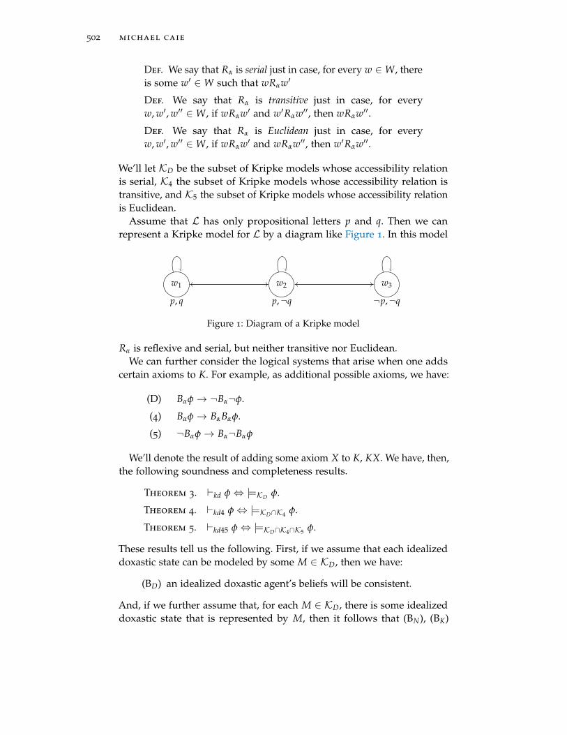
502 michael caie
Def. We say that Rα is serial just in case, for every w ∈W, thereis some w′ ∈W such that wRαw′
Def. We say that Rα is transitive just in case, for everyw, w′, w′′ ∈W, if wRαw′ and w′Rαw′′, then wRαw′′.
Def. We say that Rα is Euclidean just in case, for everyw, w′, w′′ ∈W, if wRαw′ and wRαw′′, then w′Rαw′′.
We’ll let KD be the subset of Kripke models whose accessibility relationis serial, K4 the subset of Kripke models whose accessibility relation istransitive, and K5 the subset of Kripke models whose accessibility relationis Euclidean.
Assume that L has only propositional letters p and q. Then we canrepresent a Kripke model for L by a diagram like Figure 1. In this model
w1 w2 w3
p, q p,¬q ¬p,¬q
Figure 1: Diagram of a Kripke model
Rα is reflexive and serial, but neither transitive nor Euclidean.We can further consider the logical systems that arise when one adds
certain axioms to K. For example, as additional possible axioms, we have:
(D) Bαφ→ ¬Bα¬φ.
(4) Bαφ→ BαBαφ.
(5) ¬Bαφ→ Bα¬Bαφ
We’ll denote the result of adding some axiom X to K, KX. We have, then,the following soundness and completeness results.
Theorem 3. `kd φ⇔ |=KD φ.
Theorem 4. `kd4 φ⇔ |=KD∩K4 φ.
Theorem 5. `kd45 φ⇔ |=KD∩K4∩K5 φ.
These results tell us the following. First, if we assume that each idealizeddoxastic state can be modeled by some M ∈ KD, then we have:
(BD) an idealized doxastic agent’s beliefs will be consistent.
And, if we further assume that, for each M ∈ KD, there is some idealizeddoxastic state that is represented by M, then it follows that (BN), (BK)

doxastic logic 503
and (BD) provide a complete characterization of those properties that areshared by every idealized doxastic state.
Second, if we assume that, in addition, each idealized doxastic state canbe modeled by some M ∈ KD ∩K4, then we also have:
(B4) if an idealized doxastic agent believes φ, then she willbelieve that she believes φ.
We’ll call this property positive transparency.If we further assume that, for each M ∈ KD ∩K4, there is some idealized
doxastic state that is represented by M, then it follows that (BN), (BK), (BD)and (B4) provide a complete characterization of those properties that areshared by every idealized doxastic state.
Finally, if we assume that, in addition, each idealized doxastic state canbe modeled by some M ∈ KD ∩K4 ∩K5, then we also have:
(B5) if an idealized doxastic agent fails to believe φ, then shewill believe that she fails to believe φ.
We’ll call this property negative transparency.If we further assume that, for each M ∈ KD ∩ K4 ∩ K5, there is some
idealized doxastic state that is represented by M, then it follows that (BN),(BK), (BD), (B4), and (B5) provide a complete characterization of thoseproperties that are shared by every idealized doxastic state.
In the doxastic logic literature, it is typically assumed that every ideal-ized doxastic state can be represented by some element of KD ∩K4 ∩K5,and that each element of this set accurately represents some idealized dox-astic state. Given this assumption, then, the logic governing the operatorBα is the modal logic KD45.
Note that the following principle is not assumed to hold:
(T) Bαφ→ φ.
That is, we do not assume that our idealized doxastic states are error-free.An ideal belief state, on this picture, need not be one that only includestrue beliefs.
Def. We say that Rα is reflexive just in case, for every w ∈ W,wRαw.
The axiom (T) is guaranteed to hold in any Kripke model whose accessibil-ity relation is reflexive. Importantly, then, we do not assume that a modelM representing an idealized doxastic state has a reflexive accessibilityrelation.

504 michael caie
1.2 Group Beliefs
So far, our doxastic models have treated the doxastic state of only a singleagent. This restriction, however, can be easily relaxed. Instead of a singleoperator Bα, let L now contain a series of operators Bα1 , Bα2 , . . . , Bαr . AKripke model for L will be a tuple 〈W, Rα1 , Rα2 . . . , Rαr , J·K〉, and truth-at-a-point in such a model will be defined in the obvious way. As with the caseof our individual models, we can impose various restrictions for each Rαi
such as seriality, transitivity etc. We’ll let Kα be the set of Kripke modelsfor L. We’ll let Dα, Kα
4 , Kα5 be, respectively, the set of Kripke models for L
such that each accessibility relation is serial, transitive, and Euclidean.This type of model allows us to simultaneously represent the doxastic
states of multiple agents. Furthermore, it allows us to represent certaincollective properties of the doxastic states of groups that cannot be repre-sented by a set of individual Kripke models for each agent in the group.2
Let’s consider how such features may be represented in this sort of model.In particular, we will consider how in such models we can represent thegroup doxastic properties of common belief and distributed belief.
1.2.1 Common Belief
What is it for φ be a matter of common belief amongst a group of agents?The intuitive idea is that common belief is a matter of each agent in thegroup believing φ, and each agent believing that each agent believes φ,and each agent believing that each agent believes that each agent believesφ. . . , and so on, ad infinitum.3 This sort of group doxastic property can berepresented in our models as follows.
Def. We will say that w and w′ are n-connected just in casethere is some series of worlds w1, . . . , wn+1 such that w = w1,wn+1 = w′ and for each pair 〈wi, wi+1〉 there is some Rαj suchthat wiRαj wi+1. We’ll write wRnw′ to indicate that w and w′ aren-connected.
So, for example, the set of 1-connected worlds will just be those pairsof worlds such that there is some j such that wRαj w
′, while the set of2-connected worlds will just be those pairs of worlds that are connectedvia the belief accessibility relation of at most two agents, etc.
2 See, e.g., Fagin, Halpern, and Vardi (1991), Halpern and Moses (1992), Halpern and Moses(1984), and Halpern, Moses, and Vardi (1995) for important work on the doxastic andepistemic properties of groups.
3 The concepts of common belief and common knowledge and the role that these play inreasoning were introduced in Lewis (1969). See also Aumann (1976) for another influentialearly treatment of these ideas. See Barwise (1988) for alternative analyses of the notions ofcommon belief and common knowledge.

doxastic logic 505
Let the schematic abbreviation Bαn φ be inductively characterized asfollows:
Def.
1. Bα1 φ =df Bα1 φ ∧ Bα2 φ ∧ . . . ∧ Bαr φ,
2. Bαn φ =df Bα1 Bαn−1 φ ∧ Bα2 Bαn−1 φ ∧ . . . ∧ Bαr Bαn−1 φ.
So Bα1 abbreviates the claim that each agent in the group believes φ.While Bαn abbreviates the claim that each agent in the group believes thateveryone in the group believes φ to level n− 1. As a further definitionalabbreviation, we let:
Def. Mnαφ =df Bα1 φ ∧ . . . ∧ Bαn φ.
We will read Mnαφ as saying that there is mutual belief of degree n that φ
amongst α1, . . . , αr.Given these definitions, it follows that the truth of Bαn φ and Mαn φ,
relative to a point w, in a model M, may be characterized as follows.
JBαn φKw = 1 just in case JφKw′ = 1, for every w′ such that wRnw′.
JMαn φKw = 1 just in case JφKw′ = 1, for every w′ such that there issome 1 ≤ i ≤ n such that wRiw′.
So far we haven’t added any expressive power to our language. Eachoperator Bαn and Mαn is merely an abbreviation for some formula alreadyin L. Suppose, however, that we wanted to say that φ is a matter of commonbelief amongst α1, . . . , αr. The natural way to express this is to say that,for each n, Mαn φ holds. Expressing common belief in this way, though,would require quantificational devices or devices of infinite conjunctionthat our language lacks. This doesn’t, however, mean that we can’t expressthe property of common belief in a propositional modal language. To doso, however, we need to add a new operator to our language.
Let L, then, be the language that includes, in addition to each of theoperators Bαi , an operator Cα. A Kripke model for our new language Lwill still be a tuple M = 〈W, Rα1 , Rα2 . . . , Rαr , J·K〉. Given our relations Rαi ,we can define the following relation on points in W:
Def. Let R+1 =
⋃n≥1 Rn.
R+1 is the so-called transitive closure of R1.4 Given this definition, we have
that wR+1 w′ just in case there is some n such that wRnw′. Thus wR+
1 w′
4 This is the smallest transitive relation containing R1. To see why this is a transitive relation,assume that we have w1R+
1 w2 and w2R+1 w3. Then we have that there is some n such that
w1Rnw2, i.e., w1 and w2 are n-connected. And we also have that there is some m suchthat w2Rmw3, i.e., w2 and w3 are m-connected. But, given this, it follows that we havew1Rn+mw3, i.e., w1 and w3 are (n + m)-connected.

506 michael caie
holds just in case there is some finite length path connecting w and w′ viathe accessibility relations Rαi .
Note that since R+1 is definable in terms of the Rαi ∈ M, we do not need
to include this relation in M in order to appeal to it in characterizing thetruth of certain sentences in such a model.
We can now characterize the truth of a sentence Cαφ relative to a worldof evaluation in M as follows:
JCαφKw = 1 just in case JφKw′ = 1, for every w′ such that wR+1 w′.
What are the logical properties governing the common belief operatorCα? We can characterize the logic of this operator as follows. Let Kα bethe multi-modal logic characterized by each instance (N), and the relevantinstance of (K), for each operator Bαi . (Similarly for KDα, KD4α and KD45α.)And let Kc
α (or KDcα, KD4c
α and KD45cα) be the axiomatic system we get by
adding to Kα (or KDα, KD4α and KD45α) the following axiom and rule ofinference:
(C1) Cαφ→ M1α(φ ∧ Cαφ).
(R1) `kcα
φ→ M1α(ψ ∧ φ)⇒ `kc
αφ→ Cαψ.
We, then, have the following soundness and completeness result:5
Theorem 6. `kcα
φ⇔ |=Kα φ.
Similar results show that KDcα is sound and complete with respect to Dα,
that KD4cα is sound and complete with respect to Dα ∩Kα
4 , and that KD45cα
is sound and complete with respect to Dα ∩Kα4 ∩Kα
5 . The logic governingCα, then, is characterized by adding (C1) and (R1) to the axioms governingthe operators Bαi .
Now it’s clear that the structural properties of the accessibility relationR+
1 will supervene on the structural properties of the accessibility relationsRαi . Importantly, though, the structural properties of R+
1 may be distinctfrom those of Rαi . In certain cases, R+
1 may have additional structural prop-erties to those of Rαi , while in other cases, R+
1 may lack certain structuralproperties had by each of the Rαi . Given such discrepancies, then, thelogic governing common belief may be distinct from the logic governingindividual belief. Let’s consider, briefly, some ways in which commonbelief may inherit some of the logical properties governing individualbelief and some ways in which the logic governing common belief maycome apart from the logical properties governing individual belief.
First, note that the transitive closure of a serial relation is also serial.If, then, each Rαi is serial, R+
1 will also be serial. And so, if the logic
5 See Halpern and Moses (1992) for a proof of this. Halpern and Moses (1992), in fact,includes an additional axiom stating M1
αφ ↔ (Bα1 φ ∧ . . . ∧ Bα1 φ). This, however, is adefinitional truth and so is not strictly speaking required as an axiom.

doxastic logic 507
governing individual beliefs includes the principle (D), then so will thelogic governing common belief. Thus, if the individual agents that we arerepresenting are such that their beliefs are guaranteed to be consistent,then so too will the common beliefs of this group.
We have, then:
(D) |=Dα Cαφ→ ¬Cα¬φ.
Next, note that, given its definition, R+1 is guaranteed to be transitive. In
particular, it will satisfy this property whether or not all Rαi do. In thismanner, then, R+
1 may have a structural feature that some Rαi lack. Giventhat R+
1 is transitive, we have then:
(4) |=Kα Cαφ→ CαCαφ.
Common belief, then, is guaranteed to be positively transparent, even ifindividual beliefs are not.
Finally, note that while each Rαi being serial entails that R+1 is serial,
it does not follow that if each Rαi is Euclidean then R+1 will also be Eu-
clidean.6 Thus, even if the logic of individual belief entails that individualbelief is negatively transparent, it does not follow that common belief mustalso be negatively transparent.
1.2.2 Distributed Belief
What is it for φ to be a matter of distributed belief? The intuitive idea isthat φ is a distributed belief amongst some group of agents just in case φ
is a consequence of what all of the agents believe.To express this notion, we’ll introduce the operator Dα to our language L.
A model for L will still be a tuple M = 〈W, Rα1 , Rα2 . . . , Rαr , J·K〉. We definethe following relation amongst the members of W, given our relations Rαi .
Def. Let wRdw′ just in case for every Rαi , wRαi w′.
Truth-at-a-world for a formula Dαφ, in a model M, can, then, be character-ized as follows:
JDαφKw = 1 just in case JφKw′ = 1, for every w′ such that wRdw′.
We can characterize the logic of this operator as follows. Again let Kα bethe multi-modal logic characterized by each instance (N), and the relevantinstance of (K), for each operator Bαi . And let Kd
α be the axiomatic systemwe get by adding to Kα the relevant instance of (K) for the operator Dα, aswell an axiom of the following form, for each αi:
(D1) Dαφ→ Bαi φ.
We, then, have the following soundness and completeness result:7
6 See Lismont and Mongin (1994), Colombetti (1993), and Bonanno and Nehring (2000) forproofs and discussion of this result.
7 See Halpern and Moses (1992).
508 michael caie
Theorem 7. `kdα
φ⇔ |=Kα φ.
Similarly, if we let K4α (K45α) be the the multi-modal logic characterizedby each instance (N), and the relevant instances of (K) and (4) (and (5)), foreach operator Bαi , and let K4d
α (K45dα) be the axiomatic system we get by
adding to K4α (K45α) the relevant instances of (K) and (4) (and (5)) for theoperator Dα, then we can also show that K4d
α (K45α) is sound and completewith respect to Kα
4 (Kα4 ∩Kα
5).It’s clear that the structural properties of Rd will supervene on the struc-
tural properties of the accessibility relations Rαi . While, though, Rd mayinherit certain structural properties from Rαi , other structural propertiesof Rd may be distinct from those of Rαi .
First, note that if each Rαi is transitive, then Rd is transitive. Similarly, ifeach Rαi is Euclidean, then Rd is Euclidean. It’s for this reason that if thelogic governing the Bαi includes the principles (4) or (5), so too will thelogic governing Dα.
Importantly, however, it doesn’t follow from the fact that each Rαi isserial, that Rd is also serial. For it doesn’t follow from the fact that, foreach w, and each Rαi , there is w′ such that wRαi w
′, that for each w there issome w′ such that wRdw′. For while, for some w, it may be the case that,for each Rαi , there is some w′ such that wRαi w
′, this w′ need not be thesame in each case. Even, then, if the logic governing each Bαi includes theprinciple (D), it doesn’t follow this will be a principle governing Dα. Even,then, if each individual’s beliefs are consistent, the distributed beliefs ofthe group need not be.
1.3 Some Remarks on the Interpretation of the Formalism
So far, we’ve been assuming that our doxastic models represent the doxas-tic states of certain idealized agents. And, as we’ve noted, there is a standardassumption in the literature that the logic governing such states is KD45.It would, however, be a mistake, I think, to take there to be a substantivequestion of whether or not the logic governing idealized doxastic statesreally is KD45 or some other logic. Instead, I think it is much more naturalto think of these principles as simply codifying a certain idealization. Onthis view, then, there are various types of idealized doxastic states that wemight investigate. For example, we might consider those doxastic statesthat can be represented by some model in K. Doxastic states of this typewould be logically omniscient and closed under logical consequence, butperhaps not consistent or perhaps not positively or negatively transpar-ent. Or we might consider those doxastic states that can be representedby some model in K ∩ D ∩ K4. Doxastic states of this type would belogically omniscient, closed under logical consequence, consistent and

doxastic logic 509
positively transparent, but not negatively transparent. And so on. Nowdifferent types of idealized doxastic states may be useful or illuminatingfor different purposes, but it seems implausible to me that any one ofthese idealizations stands out as being of significantly greater theoreticalimportance than all of the others.
One might, however, endorse the bolder hypothesis that our doxasticmodels are, in fact, intended to represent necessary features of any possi-ble doxastic state. Given this view, the question of whether such modelsare appropriate and, if so, which constraints should be endorsed, becomesa substantive question. Some have, indeed, argued that the nature of dox-astic states makes it the case that they may be represented by models inK.8 Others have argued that the nature of doxastic states makes it the casethat principles such as (B4) and (B5) will be satisfied and so models inK4 or K5 may serve to represent such states.9 These claims, however, arequite controversial, and it would take us too far afield now to assess theirplausibility.10 Suffice it to say, there are certain accounts of the nature ofdoxastic states according to which such states may in fact be accuratelyrepresented by the sorts of models we’ve been considering, while, accord-ing to other accounts, certain doxastic states—indeed the types of doxasticstates that actual agents tend to have—cannot be accurately representedby the sorts of models that we’ve been considering.
A third way of interpreting our doxastic models, which should bedistinguished from the first interpretation, has it that the role of this classof models is to codify certain general principles that a rational agent’sdoxastic state ought to satisfy. Here we might profitably consider, as ananalogous view, the Bayesian account of credal rationality. Accordingto a subjective Bayesian, the class of probability functions defined oversome algebra A represents the class of rationally permissible credal statesdefined over A. Those features, then, that are common to all such functionsrepresent rational requirements on any credal state defined over such analgebra. Similarly, one might hold that the class of models K (or the classK∩D∩K4 etc.) represent the class of rationally permissible doxastic states.Those features, then, that are common to this class, i.e., the valid formulas
8 See e.g., Stalnaker (1984), Lewis (1974), and Lewis (1999). Both Stalnaker and Lewis,however, recognize that there must be a sense in which agents may have contradictorybeliefs or fail to have beliefs that are closed under logical consequence. Lewis (2000) arguesthat we may think of an agent’s doxastic state as consisting of various fragments, whereeach fragment may be represented by a possible worlds model. An agent, then, may haveinconsistent beliefs by having fragments that disagree, and the agent may have beliefs thatfail to be logically closed by believing, say, φ relative to one fragment and φ→ ψ relativeto another, but not believing ψ relative to any fragment.
9 See, for example, Shoemaker (1996a, 1996b) for arguments that, at least in certain cases,positive introspection should hold as a constitutive matter.
10 The arguments in Williamson (2000), for example, put serious pressure on the idea thatthe transparency principles (B4) and (B5) will hold for actual agents.

510 michael caie
given the class of models, represent, on this view, rational requirementson any doxastic state.
Now this view may seem to be a mere notational variant on the firstinterpretation. However, concluding this would, I think, be a mistake.What an actual agent ought to believe and what an idealized agent wouldbelieve are not the same thing. Here’s a somewhat facile, but I thinksufficiently instructive example that illustrates this point. An idealizedagent would, plausibly, believe that they are idealized. However, a rationalagent, who is not an idealized agent, should not be rationally required tobelieve that they are idealized. Thus, a representation of what an idealizeddoxastic state would look like is not, thereby, a representation of whatdoxastic features a rational agent ought to have.
The view that our doxastic models serve to codify rational requirementson doxastic states, again, makes it a substantive question which class ofKripke models, if any, we should take as the appropriate class for formu-lating our doxastic logic. One may, for example, maintain that doxasticstates ought to be such that they’re consistent and closed under logicalentailment, but deny that doxastic states ought to be transparent on painof irrationality. Once again, the issues here are subtle and we will simplycontent ourselves with flagging the issues, without making any attempt toresolve them.
Having noted these three possible roles that our doxastic models mayplay, it is worth highlighting that different classes of models might, infact, play different roles. So, for example, one might maintain that theclass K is the smallest class that serves to characterize how a rationalagent’s doxastic state ought to be. But one might still find it profitable toinvestigate what features are exhibited by the sorts of idealized doxasticstates characterized by, say, K ∩D ∩K4.
In what follows, I will often continue to speak as if the Kripke models,as well as other models we’ll introduce, are meant to represent idealizeddoxastic states. However, in certain cases a normative or descriptive in-terpretation may seem more natural and so I will sometimes talk as ifthe models in question are meant to describe such facts. In each case,though, it is worth bearing in mind the alternative interpretations that areavailable.
2 belief revision
So far we’ve seen how to represent certain features of idealized doxasticstates. In particular, we’ve seen how to represent the beliefs of an idealizeddoxastic agent, including beliefs about that agent’s beliefs, as well as beliefsabout other agents’ beliefs. The models that we’ve looked at, however, saynothing about how idealized doxastic states should change given new

doxastic logic 511
information. In this section we’ll look at an influential account of beliefrevision called AGM.11
The basic theory of AGM consists of a set of formal postulates that serveto codify rational constraints on belief revision, expansion and contraction.In addition to such formal postulates, however, various authors haveprovided models of how functions meeting these constraints may bedetermined. We’ll begin, in Section 2.1, by considering the basic postulatesof AGM. In Section 2.2, we’ll then consider some possible connectionsbetween rational belief revision, expansion and contraction. In Section 2.3,we’ll consider some models for belief revision and contraction. And, finally,in Section 2.4 we’ll look at some additional postulates that have beenproposed to handle the phenomenon of iterated belief revision.
2.1 AGM: The Basic Postulates
Let L be a set of sentences closed under the standard Boolean operators,and let Γ ⊆ L be a set of such sentences. We’ll denote by Cl(Γ) the logicalclosure of Γ. In standard presentations of this theory, it is assumed thatrational agents have belief states that can be (at least partially) modeledby logically closed sets of sentences. In this section, we will follow thispractice as well. Note that this marks a departure from our treatmentsof belief states in the previous section, where such states were modeledas sets of possible worlds. We’ll let B be a possible belief set, i.e, a set ofsentences such that B = Cl(B). We denote the set of belief sets B.
We’ll first consider the AGM postulates governing rational belief expan-sion. We let + : B ×L → B be a function mapping pairs of belief sets andsentences to belief sets. We’ll let B+
φ be the result of applying the function+ to the belief set B and sentence φ. According to AGM, rational beliefexpansions must satisfy the following constraints.
(B+1 ) φ ∈ B+
φ .
(B+2 ) B ⊆ B+
φ .
(B+3 ) If φ ∈ B, then B = B+
φ .
(B+4 ) If A ⊆ B, then A+
φ ⊆ B+φ .
(B+5 ) For any operation # satisfying B+
1 –B+4 , B+
φ ⊆ B#φ.
We can think of expansion as an operation that increases the agentsbelief set B to accommodate belief in φ. Then (B+
1 ) tells us that, given this
11 This account developed out of Alchourrón et al. (1985). For a comprehensive survey seeGärdenfors (1988). See also Huber (this volume) for a helpful treatment of this and otherrelated material.

512 michael caie
operation, φ will be a part of the resultant belief set. While (B+2 ) tells us
that everything that was believed prior to the operation is believed afterthe operation. Also (B+
3 ) tells us that, if φ is already believed, given B,then the expansion operation is trivial. Additionally (B+
4 ) tells us that theexpansion operation is monotone, i.e., that it preserves the subset relation.And, finally, (B+
5 ) tells us that, in a specific sense, expansion is the mostconservative operation with the preceding characteristics.
It can be shown that (B+1 )–(B+
5 ) uniquely pin down the expansion opera-tor. Thus:
Theorem 8. A function + satisfies (B+1 )–(B+
5 ) just in case B+φ =
Cl(B ∪ φ).12
Next, we consider belief revision. We let ∗ : B × L → B be a functionmapping pairs of belief sets and sentences to belief sets. According toAGM, rational belief revisions must satisfy the following constraints.
(B∗1) φ ∈ B∗φ.
(B∗2) B∗φ ⊆ B+φ .
(B∗3) If ¬φ 6∈ B, then B+φ ⊆ B∗φ.
(B∗4) B∗φ = L just in case |= ¬φ.
(B∗5) If |= φ↔ ψ, then B∗φ = B∗ψ.
(B∗6) B∗φ∧ψ ⊆ (B∗φ)+ψ .
(B∗7) If ¬ψ 6∈ B∗φ, then (B∗φ)+ψ ⊆ B∗φ∧ψ.
Like expansion, we can think of revision as an operation that changes anagent’s belief set B to accommodate belief in φ. Unlike expansion, though,in belief revision certain beliefs may be discarded to accommodate φ.
Constraint (B∗1) tells us that, given this operation, φ will be a part ofthe resultant belief set. While (B∗2) tells us that everything that is believedgiven belief revision will be believed given belief expansion. Also (B∗3)tells us that the reverse is also true, and so expansion and revision deliverthe same output, when φ is logically compatible with B. And (B∗4) tell usthat that the result of belief revision will be a consistent belief set just incase φ is itself logically consistent. Constraint (B∗5) tells us that logicallyequivalent sentences induce the same revision operation on a belief set.And (B∗6) tells us that everything that is believed after revising a belief setgiven a conjunction φ ∧ ψ, will be believed after first revising the samebelief set given φ and then expanding the resultant belief set given ψ.
12 See Gärdenfors (1988).

doxastic logic 513
Finally, (B∗7) tell us that the reverse is true, and so revising given φ andthen expanding given ψ delivers the same output as revising given φ ∧ ψ,when ψ is consistent with the result of revision given φ.
Unlike with the constraints on +, these constraints do not suffice touniquely determine the function ∗. Instead, there is a non-empty, non-singleton, set of functions that satisfy (B∗1)–(B∗7).
Finally, we consider belief contraction. We let − : B × L → B be afunction mapping pairs of belief sets and sentences to belief sets. Accordingto AGM, rational belief contractions must satisfy the following constraints.
(B−1 ) B−φ ⊆ B.
(B−2 ) If φ 6∈ B, then B−φ = B.
(B−3 ) If 6|= φ, then φ 6∈ B−φ .
(B−4 ) If φ ∈ B, then B ⊆ (B−φ )+φ .
(B−5 ) If |= φ↔ ψ, then B−φ = B−ψ .
(B−6 ) B−φ ∩ B−ψ ⊆ B−φ∧ψ.
(B−7 ) If φ 6∈ B−φ∧ψ, then B−φ∧ψ ⊆ B−φ .
We can think of contraction as an operation that changes an agent’sbelief set B to accommodate the removal of a belief φ.
Constraint (B−1 ) tells us that belief contraction does not introduce anynew beliefs. While (B−2 ) tells us that if the agent does not already believe φ,then the result of contracting by φ leaves the agent’s belief set unchanged.Then (B−3 ) tells us that if φ is not a logical truth, then φ will not be inany belief set that is contracted by φ. And (B−4 ) tells us that if a beliefset B contains φ, then the result of contracting this belief set by φ andthen expanding the resulting set by φ will contain everything that is inB. Next (B−5 ) tells us that logically equivalent sentences induce the samecontraction operation on a belief set. And (B−6 ) tells us that every beliefthat remains when a belief set is contracted by φ and by ψ will remainwhen the belief set is contracted by φ ∧ ψ. Finally, (B−7 ) tells us that if φ isnot in the belief set that results from contracting a belief set B by φ ∧ ψ,then everything that results from contracting B by φ ∧ ψ will be in the setthat result from contracting B by φ.
As with the constraints on ∗, these constraints do not uniquely determinethe function −. Again, there is a non-empty, non-singleton set of functionsthat satisfy each of (B−1 )–(B−7 ).

514 michael caie
2.2 Relations Between Operations
Given these rational constraints on contraction, revision and expansion,it is natural to ask what connections there might be between these threeoperations. In this section, we’ll consider some possible options.
So far we’ve been talking as if agents adopt distinct policies of rationalbelief revision, contraction and expansion. Following Levi (1977), however,one might maintain that agents only really adopt policies of contractionand expansion, and that a policy of revision is determined by the lattertwo policies in the following manner.
Constitutive Levi Identity. B∗φ =df (B−¬φ)+φ .
If the claim that the adoption of a rational revision policy simply consistsin the adoption of rational contraction and expansion policies is to be at allplausible, it must be the case that, given the putative analysis, it is ensuredthat the resulting revision policy will indeed be rational given that thecontraction and expansion policies are. The following result shows that,given the Constitutive Levi Identity, this is so.
Theorem 9. If − satisfies (B−1 )–(B−3 ) and (B−5 )–(B−7 ), and +
satisfies (B+1 )–(B+
5 ), then, given the Constitutive Levi Identity,∗ satisfies (B∗1)–(B∗7).13
Now even if one wants to reject the claim that the adoption of a belief re-vision policy simply consists in the adoption of expansion and contractionpolicies, one should, I think, nonetheless hold that there are importantrational constraints governing which policies of belief revision, expansionand contraction an agent may simultaneously adopt. In particular, whetherone thinks that rational belief revision should be analyzed in terms of ra-tional belief contraction and expansion, one should, I think, endorse thefollowing normative constraint.
Normative Levi Identity. If ∗ is an agent’s revision policy,− her contraction policy, and + her expansion policy, then theagent ought to be such that B∗φ = (B−¬φ)
+φ .
Two points are worth mentioning here.First, the Normative Levi Identity does, indeed, impose a substantive
constraint in addition to those imposed by (B+1 )–(B+
5 ), (B∗1)–(B∗7), and (B−1 )–(B−7 ). For there are functions +, ∗ and − that satisfy (B+
1 )–(B+5 ), (B∗1)–(B∗7),
and (B−1 )–(B−7 ), respectively, but that fail to jointly satisfy the conditionthat B∗φ = (B−¬φ)
+φ .14
13 See Gärdenfors (1988), ch. 3.6.14 This follows from the fact that there is a unique function + satisfying conditions (B+
1 )–(B+5 ),
together with the fact that there are multiple functions ∗ and − satisfying (B∗1)–(B∗7), and(B−1 )–(B−7 ) respectively.

doxastic logic 515
Second, Theorem 9 guarantees that the constraints imposed by theNormative Levi Identity are, indeed, consistent with the constraintsimposed by (B+
1 )–(B+5 ), (B−1 )–(B−7 ), and (B∗1)–(B∗7). For there are functions −
and + that satisfy the constraints imposed by (B−1 )–(B−7 ), and (B+1 )–(B+
5 ),and it follows from this fact, together with Theorem 9 that, given suchfunctions, there is a function ∗ that satisfies the constraints imposed by(B∗1)–(B∗7), and, in addition, is such that B∗φ = (B−¬φ)
+φ .
Another option, following Harper (1976), is to maintain that agents onlyreally adopt policies of revision and expansion. In particular, one maymaintain that an agent’s policy of contraction is determined by her policyof revision as follows.
Constitutive Harper Identity. B−φ =df B ∩ B∗¬φ.
If the claim that the adoption of a rational contraction policy simplyconsists in the adoption of a rational revision policy is to be at all plausible,it must the case that, given the putative analysis, it is ensured that theresulting contraction policy will indeed be rational given that the revisionpolicy is. The following result shows that, given the Constitutive Harper
Identity, this is so.
Theorem 10. If ∗ satisfies (B∗1)–(B∗7), then, given the Constitu-tive Harper Identity, − satisfies (B−1 )–(B−7 ).15
Now, again, even if one wants to reject the claim that the adoption ofa belief contraction policy simply consists in the adoption of a revisionpolicy, one should, I think, still hold that there are important rationalconstraints governing which contraction and revisions policies an agentmay simultaneously adopt. In particular, whether one thinks that rationalbelief contraction should be analyzed in terms of rational belief revision,one should, I think, endorse the following normative constraint:
Normative Harper Identity. If ∗ is an agent’s belief revisionpolicy, and − her belief contraction policy, then the agent oughtto be such that B−φ = B ∩ B∗¬φ.
Two points are, again, worth mentioning here.First, the Normative Harper Identity provides a substantive constraint
in addition to (B∗1)–(B∗7) and (B−1 )–(B−7 ). For there are functions ∗ and −that satisfy the latter constraints but for which the identity B−φ = B ∩ B∗¬φ
fails to hold.16
Second, Theorem 10 guarantees that the constraint imposed by theNormative Harper Identity is consistent with the constraints imposed
15 See Gärdenfors (1988) ch. 3.6.16 This follows from the fact that there are multiple functions ∗ and − satisfying (B∗1)–(B∗7),
and (B−1 )–(B−7 ) respectively.

516 michael caie
by (B∗1)–(B∗7) and (B−1 )–(B−7 ). For there is some function ∗ satisfying (B∗1)–(B∗7), and so, given Theorem 10, it follows that there is some other function− satisfying (B−1 )–(B−7 ), such that B−φ = B ∩ B∗¬φ.
2.3 AGM: Models
Constraints (B−1 )–(B−7 ) determine a class of rational contraction functions,while (B∗1)–(B∗7) determine a class of rational revision functions. Thereare, however, other ways of characterizing the classes determined by(B−1 )–(B−7 ) and (B∗1)–(B∗7). In particular, we can provide models of possiblefeatures of an agent’s doxastic state that might serve to determine whichrational revision or contraction policy she adopts, and we can show that,given certain rational constraints on such features, the classes of rationallypermissible revision or contraction functions are the same classes as thosedetermined by (B−1 )–(B−7 ) and (B∗1)–(B∗7).
2.3.1 Sphere Systems
We first consider a model of how an agent’s doxastic state might serveto determine a rational revision policy.17 In rough outline, we may thinkof an agent’s doxastic state, in addition to determining a belief set, asalso determining, for each possible belief set B, an ordering of plausibilityamongst various maximal consistent descriptions of how the world mightbe. Given a doxastic state with such structure, we may think of the agent asadopting a revision policy such that, given a belief set B and a sentence φ,the resulting revised belief set is just the intersection of the most plausiblemaximal consistent descriptions of how the world might be that contain φ.
A little more pedantically: Let W be the set of maximal consistentsubsets of L. Following the literature, we’ll refer to these as possible worlds.It is, however, worth keeping in mind that, as sets of of sentences, thesediffer from the possible worlds considered in the previous section. For anybelief set B, we let JBK = w ∈ W : B ⊆ w. And for any P ⊆ W , we letBP = ∩w : w ∈ P.
Let S be a set of subsets ofW . We call S a system of spheres centered on Bjust in case S satisfies the following conditions.
Ordering. For every S, S′ ∈ S, either S ⊆ S′ or S′ ⊆ S.
Centering. JBK ∈ S, and for every S ∈ S, JBK ⊆ S.
Universality. W ∈ S.
Limit Assumption. Let φ be a sentence. If there is some S ∈ Ssuch that S ∩ JφK 6= ∅, then there is some S ∈ S such that (i)
17 See Grove (1988) for the initial development of this model. The model is, in certain respects,notably similar to the semantic theory for counterfactuals developed in Lewis (1973).

doxastic logic 517
S ∩ JφK 6= ∅, and (ii) for every S′ ∈ S such that S′ ∩ JφK 6= ∅,S ⊆ S′.
Ordering tells us that the members of S can be totally ordered bythe subset relation. Centering tells us that the set of worlds that arecompatible with the belief set B is a member of S that is minimal withrespect to the subset ordering on S. Universality tells us that the set ofall worlds is itself a member of S. And, finally, the Limit Assumption tellsus that for any sentence φ if the set of S ∈ S such that φ is true at someworld in S is non-empty, then this set has a least element relative to thesubset ordering on S.
If 6|= ¬φ, then we let Sφ be the smallest sphere intersecting φ. GivenUniversality and the Limit Assumption, such a sphere is guaranteed toexist. And if |= ¬φ, then we let Sφ =W . We let CS(φ) = JφK∩ Sφ.
Let S be a function that maps each B ∈ B to a system of spherescentered on B. Call this a sphere function. We denote the sphere systemdetermined by a sphere function S , for some belief set B, by SB. Finally,let f : B × L → B be a function such that there is some sphere functionS such that for every B ∈ B and φ ∈ L, f (B, φ) = ∩CSB(φ). We call this asphere revision function.
We can think of a sphere revision function, determined by some spherefunction S , as mapping a belief state B and a sentence φ to the belief statethat is determined by the worlds at which φ holds that, according to S ,are closest to B.
More precisely, we can think of a sphere revision function, determinedby some sphere function S , as operating in the following manner. Given abelief set B and a sentence φ, we first look at the sphere system centeredon B determined by S . Next we find the smallest sphere that is compatiblewith φ, and consider the set of worlds within this sphere at which φ
holds. The sphere revision function, then, returns as a belief set the set ofsentences that are true at every world within this set.
The following theorem shows that the adoption of a rational revisionfunction can always be modeled in terms of the adoption of a sphere revi-sion function determined by some sphere function S , and that, conversely,the adoption of a sphere revision function determined by some spherefunction S will always correspond to the adoption of a rational revisionfunction.
Theorem 11. Function f is a sphere revision function just incase f satisfies (B∗1)–(B∗7).18
We can support the claim that a system of spheres may be thought of asencoding a relation of doxastic plausibility as follows. Call a relation ≤overW with the following properties, a B-plausibility ordering.
18 See Grove (1988).

518 michael caie
Connectivity. For every w, w′ ∈ W , either w ≤ w′ or w′ ≤ w.
Transitivity. If w ≤ w′ and w′ ≤ w′′, then w ≤ w′′.
φ-Minimality. If JφK 6= ∅, then w ∈ JφK : w ≤ w′ for all w′ ∈JφK 6= ∅.
B-Minimality. w ≤ w′ for all w′ ∈ W just in case w ∈ JBK.
Given a B-plausibility ordering ≤, let Sw = w′ ∈ W : w′ ≤ w. We letS≤ = Sw : w ∈ W. It can be shown that:
Theorem 12. For any B-plausibility ordering ≤, S≤ is a systemof spheres centered on B, and for any system of spheres Scentered on B, there is a unique B-plausibility ordering ≤, suchthat S = S≤.19
A system of spheres, thus, encodes an ordering over possible worlds,and it is this plausibility ordering, that, according to this model, servesto determine how a rational agent will revise her belief set B given somesentence φ.
Given Theorem 10, we can also use this model to provide a modelof how an agent might adopt a rational contraction function. Given theadoption of a sphere revision function determined by some S , the agentwould adopt a policy of contracting a belief set B, given some sentence φ,so that her new belief set is given by the set of sentences that are true in alland only the worlds in CS(¬φ) ∪ JBK. That is, such an agent will contracther belief set by φ by adding to the set of worlds representing this set,the most plausible ¬φ worlds. Such a policy will be guaranteed to satisfy(B−1 )–(B−7 ).
2.3.2 Epistemic Entrenchment
Next, we consider a model of how an agent’s doxastic state might serveto determine a rational belief contraction policy.20 In rough outline, wemay think of an agent’s doxastic state, in addition to determining a beliefset, as also determining, for each belief set B, a binary relation on theset of sentences of L that encodes information about how epistemicallyentrenched such sentences are, given the belief set B. While the notion ofepistemic entrenchment is best thought of as being functionally definedvia its role in the following account of belief contraction, one can thinkof an epistemic entrenchment ordering, roughly, as corresponding to anordering representing how committed an agent is to retaining certainbeliefs, given that they have a belief set B.
19 See Gärdenfors (1988).20 See Gärdenfors and Makinson (1988) for this type of model.

doxastic logic 519
Given a doxastic state that determines an entrenchment ordering foreach belief set B, we may think of the agent as adopting a contractionpolicy such that, given a belief set B and a sentence φ, the agent restrictsB to the subset of elements ψ such that either ψ is a theorem or ψ ∨ φ ismore epistemically entrenched than φ.
A little more pedantically: let ≤ be a binary relation over L. We letφ < ψ =df φ ≤ ψ ∧ ψ 6≤ ψ. We call ≤ a B-entrenchment relation just in caseit satisfies the following postulates.
E1. If φ ≤ ψ and ψ ≤ ξ, then φ ≤ ξ.
E2. If φ |= ψ, then φ ≤ ψ.
E3. For all φ, ψ, either φ ≤ φ ∧ ψ or ψ ≤ φ ∧ ψ.
E4. If B 6= L, then φ ∈ B just in case φ ≤ ψ, for all ψ.
E5. If ψ ≤ φ, for all ψ, then |= φ.
Let : B → P(L×L) be a function that maps each B ∈ B to a binaryrelation over L. We denote each such relation by B. If each B is aB-entrenchment relation, we’ll call an entrenchment function. Let C :B ×L → B be a function such that C≤(B, φ) = ψ : ψ ∈ B and either φ <
φ ∨ ψ or |= ψ. Let f : B × L → B be a function such that there issome entrenchment function such that for every B ∈ B and φ ∈ L,f (B, φ) = C≤(B, φ). We call this an entrenchment contraction function.
The following theorem shows that the adoption of a rational contractionfunction can always be modeled in terms of the adoption of an entrench-ment contraction function determined by some entrenchment function, and that, conversely, the adoption of an entrenchment contractionfunction determined by some some entrenchment function will alwayscorrespond to the adoption of a rational contraction function.
Theorem 13. Function f is an entrenchment contraction func-tion just in case f satisfies (B−1 )–(B−7 ).21
Given Theorem 9, we can also use this model to provide a modelof how an agent might adopt a rational revision function. Given theadoption of an entrenchment contraction function determined by some, the agent would adopt the policy of revising a belief set B given φ,by first contracting B to the subset of elements ψ ∈ B such that eitherψ is a theorem or ψ ∨ ¬φ is more epistemically entrenched that ¬φ, andthen expanding the resulting set by φ. Such a policy will be guaranteed tosatisfy (B∗1)–(B∗7).
21 See Gärdenfors and Makinson (1988).

520 michael caie
2.4 Iterated Belief Revision
If an agent has adopted a revision policy ∗ satisfying (B∗1)–(B∗7), then notonly is it determined how the agent should revise her current belief set B,given some information φ, but it is also determined how the agent shouldrevise this new belief set, given additional information ψ. For a revisionpolicy satisfying (B∗1)–(B∗7) determines how any belief set should be revisedgiven any piece of information. It has, however, been suggested that theAGM postulates provide implausible results when we consider whichpatterns of iterated belief revision they count as rationally permissible andrationally mandated.22 In response to these putative problems, variousemendations of, or additions to, the AGM postulates have been suggested.In this section, we’ll consider some putative problems with iterated beliefrevision that arise for AGM and look at a few solutions that have beensuggested.
2.4.1 Problems with Iterated Belief Revision in AGM
There are two types of problems that the AGM revision postulates havebeen thought to have with iterated belief revision. On the one hand,the AGM revision postulates have been thought to be too permissive,vindicating as rational certain patterns of iterated belief revision that wouldseem to be irrational. On the other hand, the AGM revision postulateshave been thought to be too restrictive, ruling out as irrational certainpatterns of iterated belief revision that would seem to be rational. Let mesay a bit more about each of these worries in turn.
The first problem stems from the fact that (B∗1)–(B∗7) put very few con-straints on iterated belief revision. To see this, let b be some particularbelief set. We’ll, then, let (b∗1)–(b∗7) be the postulates that result from (B∗1)–(B∗7) by saturating the variable B ranging over elements of B with theparticular element b ∈ B. Then (b∗1)–(b∗7) provide constraints on a functionb∗ : L → B mapping sentences to belief sets. In particular, they provideconstraints on functions that tell us how the belief set b should be revisedgiven new information. Call such a function a b-revision function.
Def. For any function f : B × L → B, let f b be the functionsuch that < lx, by > ∈ f b ↔ < b, lx, by > ∈ f .
Def. For any function f : B × L → B, and any functiong : L → B, let f /gb : B × L → B be the function such that ifbx 6= b, then < bx, ly, bz > ∈ f ↔ < bx, ly, bz > ∈ f /gb, while< b, ly, bz > ∈ f /gb ↔ < ly, bz >∈ g.
22 See, for example, Boutilier (1996), Darwiche and Pearl (1997), and Stalnaker (2009).

doxastic logic 521
We can think of f b as the b-revision function determined by the revisionfunction f . And we can think of f /gb as the revision function that resultsfrom swapping gb for the b-revision function determined by f . We, then,have the following results.
For any f satisfying (B∗1)–(B∗7) and any b ∈ B, f b will satisfy (b∗1)–(b∗7).
For any g satisfying (b∗1)–(b∗7), and any f satisfying (B∗1)–(B∗7), f /gbwill also satisfy (B∗1)–(B∗7).
What this shows is that functions satisfying (B∗1)–(B∗7) can be thought ofas the result of freely choosing, for each b ∈ B, some function satisfying(b∗1)–(b∗7). Thus (B∗1)–(B∗7) allow us to mix-and-match b-revision functionsas we like.
This degree of freedom, however, has problematic consequences. For ab-revision function f : L → B can be seen as encoding conditional beliefs.We’ll say that the conditional belief φ|ψ is accepted by f just in caseφ ∈ f (ψ). The fact that (B∗1)–(B∗7) allow for arbitrary mixing and matchingof b-revision functions, shows that (B∗1)–(B∗7) impose almost no constraintson which conditional beliefs an agent should maintain or give up whenchanging her belief set in light of some new information.
Here’s an example that illustrates the problem.23
Flying Bird. You initially believe of some animal in the distancethat it’s neither a bird, ¬B, nor can it fly, ¬F. You, however, havethe conditional belief that it can fly, given that it’s a bird, F|B.That is, you are disposed to come to believe that the animalcan fly, were you to learn that it’s a bird. Now you learn thatthe animal can indeed fly, and as a result you give up theconditional belief F|B, and form the conditional belief ¬F|B.
This sort of transition will seem to many to be irrational. Learning thatthe consequent of a conditional belief is true would seem to provide noevidence against that conditional belief. However, this transition will besanctioned as rationally permissible given (B∗1)–(B∗7). Examples such as thishave convinced a number of authors that further constraints, in addition to(B∗1)–(B∗7), are required to adequately constrain rational revision functions.
To see why one might think that (B∗1)–(B∗7) are not only too permissivebut also too restrictive, note that if an agent adopts a revision policysatisfying (B∗1)–(B∗7), then which belief set she should have, given someinformation φ, is a function of her current belief set. This, however, has thefollowing consequence. Given the adoption of a revision policy satisfying(B∗1)–(B∗7), an agent who starts out with a belief set B and who then receives
23 This type of example and others may be found in Darwiche and Pearl (1997).
522 michael caie
a series of information ψ1, ψ2, . . . , ψ3 that she uses to successively reviseher beliefs and who, as a result, winds up, again, with belief set B, isrationally required to revise this belief set given some information φ inexactly the same manner as she would have revised this belief set, givenφ, prior to receiving the series of information ψ1, ψ2, . . . , ψ3. One might,however, think that a series of information that would ultimately leavean agent’s belief set unchanged could rationally lead to a change in theagent’s conditional beliefs.24 This sort of change, however, is ruled out asirrational by the AGM postulates.
2.4.2 Iterated Belief Revision Functions
We’ll first consider an amendment to the AGM account of rational re-vision that is meant to address the first problem. We’ll, then, consideran alternative amendment that addresses both the first and the secondproblem.
In response to worries about the excessive permissiveness of AGM,Boutilier (1996) proposes a much more restricted account of rational beliefrevision. Perhaps the simplest way to present the account is by appeal toGrove’s model in which a revision policy is represented by a set of totalpre-orders over the space of possible worlds.
Let be a function mapping each B to a B-plausibility ordering B. Aswe noted earlier, each function satisfying (B∗1)–(B∗7) may be representedby some such function . For each B, let C(B, φ) = w : φ ∈ w and w B
w′, for each w′ such that φ ∈ w′. Boutilier (1996) suggests that in orderfor to represent a rational revision function, in addition to each B
being a B-plausibility ordering, it must also satisfy the following.
Boutilier’s Constraint. C(B,φ) must be such that for allw, w′ 6∈ C(B, φ), w C(B,φ) w′ just in case w B w′.
The idea here is that a rational agent, in revising her beliefs in response tosome information φ, should adjust her plausibility ordering over worldsin such a way that the most plausible φ-worlds are ranked highest in hernew plausibility ordering but otherwise leaves the plausibility orderingamongst worlds untouched. An agent who adjusts her belief state in thismanner will effectively make the minimal adjustments to her conditionalbeliefs as is necessary in order to accommodate φ.
It is easy enough to see that the constraints that Boutilier (1996) suggestsrule out as irrational the problematic case of revision in Flying Bird.It has been argued, however, that Boutilier’s account of belief revisiondemands that too many conditional beliefs be preserved, and that this hasundesirable consequences about when an agent may be rationally required
24 For worries in this vicinity see Levi (1988) and Darwiche and Pearl (1997).

doxastic logic 523
to give up certain beliefs. Darwiche and Pearl (1997) give the followingexample.
Sequential Red Bird. You are initially uncertain aboutwhether a certain animal is a red, R, or is a bird, B. You thenget information that the animal is a bird, B. Then you getinformation, from a different source, that the animal is red, R.However, further consultation with an expert indicates that,in fact, the first piece of evidence was wrong and, in fact, theanimal is not a bird, ¬B. As a result, you wind up believingthat the animal is not a bird, ¬B, but that the animal is red, R.
Intuitively, this process of revision would seem to be perfectly rational.The constraints on revision proposed by Boutilier (1996), however, deemthis process of revision irrational. To see this, consider the following model.Let w1 = R ∧ B, w2 = ¬R ∧ B, w3 = R ∧ ¬B and w4 = ¬R ∧ ¬B. At t1,your plausibility ordering is such that:
(t1) w1 = w2 = w3 = w4.
Upon getting the information B, at t2 you minimally adjust your ordering,in accord with the Boutillier model, so that:
(t2) w1 = w2 < w3 = w4.
Then, at t3, upon getting the information R, you again minimally adjustyour ordering so that:
(t3) w1 < w2 < w3 = w4.
Finally, upon getting the information ¬B, you once again minimally adjustyour plausibility ordering, so that at t4 we have:
(t4) w3 = w4 < w1 < w2.
And so, what we find is that, upon making these minimal adjustments,you will fail to believe R, since this is a proposition that is false at someworld that is amongst the most plausible according to your plausibilityordering at t4.
The problem may be diagnosed as follows. When you start out uncertainabout R and B, you lack the conditional belief R|¬B. For, in your state atthe time, you would not come to believe that the animal is red if you wereto learn that the animal is not a bird. On the Boutillier model, however,when you get information φ, you should minimally adjust your conditionalbeliefs, i.e., you should only change your conditional beliefs insofar assuch a change is forced on you by taking what were previously the mostplausible φ-worlds to now be the most plausible worlds tout court. Since

524 michael caie
coming to believe B and then R does not force one to accept the conditionalbelief R|¬B, the Boutillier model requires that you continue to lack theconditional belief R|¬B. And so, when you come to believe ¬B, since youlack the appropriate conditional belief that would sanction your continuingto believe R, you must give up this belief.
The point that would seem to clearly emerge from this type of exampleis that if we want to allow that an agent may rationally preserve certainbeliefs that she forms over time, we need to allow the agent to adjust herconditional beliefs in certain non-minimal ways that are precluded giventhe Boutillier model.
In response to the problems of iterated revision faced, on the one hand,by Alchourrón et al. (1985), and, on the other hand, by Boutilier (1996),Darwiche and Pearl (1997) offer an alternative account of iterated revision.Their account is intended to offer stricter constraints on iterated beliefrevision than those imposed by Alchourrón et al. (1985), while allowingfor certain permissible variations in how an agent’s conditional beliefs maybe updated over time that are ruled out by Boutilier (1996). In addition,their theory is designed to accommodate the second worry about iteratedbelief revision for AGM considered in Section 2.4.1.
According to Darwiche and Pearl (1997), belief revision should not bethought of, fundamentally, in terms mapping one belief set to another.Instead, belief revision should be thought of as mapping one belief stateto another, where a belief state here is something that determines a beliefset but, in addition, encodes information about the agent’s conditionalbeliefs. We can model such a state as a plausibility ordering over the set ofpossible worlds.25
Let G be the set of belief states. For each G ∈ G, we’ll let Bel(G) be thebelief set determined by G. Let : G × L → G, be a function mappingpairs of belief states and sentences to belief states. Paralleling the AGMpostulates, Darwiche and Pearl suggest the following constraints for sucha function.
(G1) φ ∈ Bel(Gφ).
(G2) Bel(Gφ) ⊆ Bel(G)+φ .
(G3) If ¬φ 6∈ Bel(G), then Bel(G)+φ ⊆ Bel(Gφ).
(G4) Bel(Bφ) = L just in case |= ¬φ.
(G5) If |= φ↔ ψ, then Gφ = Gψ.
25 We can, of course, think of the acceptance of a belief revision function on the AGM pictureas adopting a policy for mapping one belief state to another. However, importantly, on theAGM account all that matters for this mapping is what the belief set looks like.

doxastic logic 525
(G6) Bel(Gφ∧ψ) ⊆ Bel(Gφ)+ψ .
(G7) If ¬ψ 6∈ Bel(Gφ), then Bel(Gφ)+ψ ⊆ Bel(Gφ∧ψ).
In addition, however, Darwiche and Pearl also propose the followingconstraints.
(G8) If φ |= ψ, then Bel((Gψ)φ) = Bel(Gφ).
(G9) If φ |= ¬ψ, then Bel((Gψ)φ) = Bel(Gφ).
(G10) If Bel(Gφ) |= ψ, then Bel((Gψ)φ) |= ψ.
(G11) If Bel(Gφ) 6|= ¬ψ, then Bel((Gψ)φ) 6|= ¬ψ.
Darwiche and Pearl (1997) then show how revision functions satisfyingthese constraints may be modeled. Let now be a function that mapseach belief state G to a total pre-order on the set of possible worlds G.(Again we’ll think of possible worlds as maximal consistent sets of L.) Welet w1 ≺G w2 =df w1 G w2 and w2 6G w1.
Def. We say that is a faithful assignment just in case:
(i) if Bel(G) ⊆ w1 and Bel(G) ⊆ w2, then w1 G w2 andw2 G w1;
(ii) Bel(G) ⊆ w1, Bel(G) 6⊆ w2, then w1 ≺G w2.
Let f : G × L → G. We again let BP = ∩w : w ∈ P, given a set ofworlds P. And for each G ∈ G, and each we let C(G, φ) = w : φ ∈w and w G w′, for each w′ such that φ ∈ w′. Darwiche and Pearl (1997)show:
Theorem 14. Function f satisfies (G1)–(G7) just in case thereexists a faithful assignment such that Bel(G f
φ) = BC(G,φ).
In addition, Darwiche and Pearl (1997) show:
Theorem 15. If f satisfies (G1)–(G7), then f satisfies (G8)–(G11)just in case f and any corresponding faithful assignment such that Bel(G f
φ) = BC(G,φ) satisfy:
(iii) if φ ∈ w1 and φ ∈ w2, then w1 G w2 if and only ifw1 G f
φw2;
(iv) if ¬φ ∈ w1 and ¬φ ∈ w2, then w1 G w2 if and only ifw1 G f
φw2;
(v) if φ ∈ w1 and ¬φ ∈ w2, then if w1 ≺G w2, then w1 ≺G fφ
w2;
(vi) if φ ∈ w1 and ¬φ ∈ w2, then if w1 G w2, then w1 G fφ
w2.

526 michael caie
Given Theorem 14 and Theorem 15, we can think of an agent’s beliefstate as being representable by a total pre-order over the space of possibleworlds, while the agent’s rational revision policy may be represented asa function mapping a pair of such a pre-order and a sentence to anotherpre-order. A rational revision policy will be representable by a function, ,that maps each such pre-order, G, and each sentence, φ, to a pre-order Gφ,such that:
the minimal worlds in Gφ are the minimal φ-worlds in G;
the ordering amongst the φ-worlds in Gφ is exactly the ordering ofthe φ-worlds in G;
the ordering amongst the ¬φ-worlds in Gφ is exactly the ordering ofthe ¬φ-worlds in G;
any strict or weak preference for a φ-world w1 over a ¬φ-world w2
in G is preserved in Gφ.
Note, however, that the Darwiche and Pearl’s account does not requirethat strict or weak preferences for ¬φ-worlds over φ-worlds, given G, bepreserved in Gφ. More specifically, unlike on the Boutillier model, theDarwiche and Pearl account allows that a φ-world w1, which is non-minimal in G and which may not be strictly preferable to some ¬φ-worldw2 may be strictly preferable to w2 relative to Gφ. And this allows Darwicheand Pearl to deal with the problematic case Sequential Red Bird.
Again let w1 = R ∧ B, w2 = ¬R ∧ B, w3 = R ∧ ¬B and w4 = ¬R ∧ ¬B.At t1, your plausibility ordering is such that:
(t′1) w1 = w2 = w3 = w4.
And, again, given the Darwiche and Pearl model, upon getting the infor-mation B, at t2 you will adjust your ordering so that:
(t′2) w1 = w2 < w3 = w4.
At t3, however, upon getting the information R, the Darwiche and Pearlmodel allows you to adjust your ordering such that:
(t′3) w1 < w2 < w3 < w4.
Compare this to the ordering that is required by the Boutillier model:w1 < w2 < w3 = w4. The key difference here is that, upon getting theinformation R, Boutilier (1996) requires that you only promote the mostplausible R-world. Darwiche and Pearl (1997), however, allows that each ofthe R-worlds may be promoted. And, given the ordering w1 < w2 < w3 <
w4, upon getting the information ¬B at t4 you will adjust your orderingso that:

doxastic logic 527
(t′4) w3 < w4 < w1 < w2.
And so what we find is that at the end of this process you will believe ¬Band you will believe R.
The postulates proposed in Darwiche and Pearl (1997), however, are notwithout problems. In particular, (G9) would seem to be subject to potentialcounterexamples. Thus consider the following case:26
Conjunctive Red Bird. You are initially uncertain aboutwhether a certain animal is a red, R, or is a bird, B. Moreoveryou start out assuming that information about whether ornot the animal is a bird, gives you no information about theanimal’s color. In particular, you do not have the conditionalbelief R|¬B. You then get information that the animal is ared bird, R ∧ B. However, further consultation with an expertindicates that, in fact, the animal is not a bird, ¬B. As a result,you wind up believing that the animal is not a bird, ¬B, butthat the animal is red, R.
Intuitively this would seem to be a rational progression of belief revision.This progression, however, is ruled out as irrational given (G9). To see this,note that since ¬B is incompatible with R ∧ B, (G9) requires that the resultof your revising, given ¬B, the belief state you have after incorporatingR∧ B, be the same as the belief state that would have resulted had you firstgotten the information ¬B. But since you start out lacking the conditionalbelief R|¬B, (G9), then, precludes your continuing to believe R once youaccept ¬B.
The problem here would seem to be that upon getting some information,say R ∧ B, it may be rational for one to take various parts of that informa-tion to be independent of others in the sense that one takes it that one partis true, conditional on some other part turning out to be false. But (G9)precludes assuming this sort of independence. It’s hard to see, however,why such assumptions of independence should be rationally precluded.
3 dynamic doxastic logic
The models developed in Section 1 allowed us to represent an agent’sbeliefs, including various higher-order beliefs about the agent’s own beliefs.Those models, however, failed to represent important features of an agent’sdoxastic state. In particular, they failed to provide any representation of anagent’s conditional beliefs. The AGM models, on the other hand, allowedus to capture this feature of an agent’s doxastic state. However, the AGM
26 See, e.g., Stalnaker (2009) for this type of example.

528 michael caie
models failed to provide any representation of an agent’s higher-orderbeliefs.
In this section, we’ll begin by presenting models, in the style of Hintikka,that allow us to represent both an agent’s unconditional beliefs and herconditional beliefs, and also allow us to represent various higher-orderconditional and unconditional beliefs. We’ll, then, consider how to addto the language dynamic operators that serve to express how an agent’sbeliefs, both conditional and unconditional, would be revised in light ofnew information.
3.1 Doxastic Plausibility Models
Let L be a propositional language including the standard Boolean connec-tives. In addition, we’ll assume that L contains a binary operator Bα(·, ·).As a notational simplification, we will write the second argument as asuperscript, so that Bα(φ, ψ) =df Bψ
α φ. The intuitive gloss of Bψα φ will be
“Alpha believes φ, conditional on ψ.”A plausibility model for L is a tuple M = 〈W,≤, J·K〉. W, as before, is a
set of worlds, and J·K is the interpretation function mapping propositionalletters to sets of possible worlds. ≤ is a ternary relation on W. We writethis as: w1 ≤w w2. The intuitive gloss on this is that, relative to Alpha’splausibility ordering in w, w1 is at least as plausible as w2. We assume that,for each w, ≤w is connected, transitive and satisfies φ-minimality. For easeof reference, we list these conditions again.
Connectivity. For every w′, w′′ ∈ W , either w′ ≤w w′′ orw′′ ≤w w′.
Transitivity. If w′ ≤w w′′ and w′′ ≤w w′′′, then w′ ≤w w′′′.
φ-Minimality. For each Q ⊆ W such that Q 6= ∅, w′ ∈ Q :w′ ≤w w′′, for all w′′ ∈ Q 6= ∅.
The truth of a sentence φ at a world w in a plausibility model M maybe defined inductively in the standard manner. Here we simply give thecondition for Bψ
α (φ).
Def. JφKm =df w : JφKwm = 1.
Def. For each Q ⊆ W, we let Min≤w(Q) =df w′ ∈ Q : w′ ≤w
w′′, for all w′′ ∈ Q
We then say:
JBψα φKw
m = 1 just in case Min≤w(JψKm) ⊆ JφKm.
We’ll take the notion of unconditional belief to be defined in terms ofconditional belief as follows:
doxastic logic 529
Def. Bαφ = B>α φ.
Our models here, of course, look quite a lot like the Grove models fromSection 2.3.1. There are, however, some differences that are worth high-lighting. One, not terribly important, difference is that, in these models,we once again take possible worlds to be primitive entities, instead of max-imally consistent sets of sentences. Another, more significant, difference isthat our doxastic plausibility models, unlike the Grove models, are definedfor a language with an iterable operator that expresses conditional belief.Our models, then, are able to represent the conditional and unconditionalbeliefs of an agent who has conditional and unconditional beliefs abouther own conditional and unconditional beliefs.
We can provide an axiomatic theory for our language L that is sound andcomplete with respect to the class of plausibility models so characterized.We’ll call this theory C.
Axioms of C
(C1) Bφα φ.
(C2) (Bφα ψ ∧ Bψ
α φ)→ (Bφα ξ ↔ Bψ
α ξ).
(C3) (Bφ∨ψα φ) ∨ (Bφ∨ψ
α ψ) ∨ (Bφ∨ψα ξ ↔ (Bφ
α ξ ∧ Bψα ξ)).
Inference Rules of C
(TI) If (φ1 ∧ . . . ∧ φn) → ψ is a tautology, then `c φ1 ∧. . . ∧ φn ⇒ `c ψ.27
(DWC) If `c (φ1 ∧ . . . ∧ φn) → ψ then `c (Bξαφ1 ∧ . . . ∧
Bξαφn)→ Bξ
αψ.
Axiom (C1) tells us that, for every φ, Alpha believes φ conditional onφ. Axiom (C2) tells us that if Alpha believes ψ conditional on φ, and φ
conditional on ψ, then, for any ξ, Alpha believes ξ conditional on φ justin case they believe ξ conditional on ψ. Axiom (C3) tells us that Alpha issuch that, conditional on φ ∨ ψ, either they believe φ, or they believe ψ,or, for every ξ, they believe ξ just in case they believe ξ conditional on φ
and conditional on ψ. Rule (TI) tells us that the system C is closed underlogical entailment. And, finally, (DWC) tells us that Alpha’s conditionalbeliefs are closed under entailment given C.
Let P be the set of plausibility models satisfying the constraints we’velaid down. We, then, have the following result.
Theorem 16. `c φ⇔ |=P φ.28
27 It is assumed, for both rules, that if n = 0, then (φ1 ∧ . . . ∧ φn) = >, and so the conditional(φ1 ∧ . . . ∧ φn)→ ψ is equivalent to ψ.
28 For a proof of this result see Lewis (1971). Lewis’ proof concerns the logic of conditionals,but the same proof applies when we replace the conditional φ > ψ with Bφ
α (ψ).

530 michael caie
As with the case of our earlier Kripke models, we can characterizesubsets of P by imposing constraints on the plausibility relation ≤.
Def. We say that ≤ is minimally homogeneous just in case forevery w, every z ∈ Min≤w(W) is such that ≤w=≤z. Def. Wesay that ≤ is minimally weakly homogeneous just in case for everyw, every z ∈ Min≤w(W) is such that if w1 6<w w2 then w1 6<z
w2.
Let PH be the members of P such that ≤ is minimally homogeneous.And let PWH be the members of P such that ≤ is minimally weakly homo-geneous. Now consider the following positive and negative introspectionprinciples.
(C4) Bφα (ψ)→ Bα(Bφ
α (ψ)).
(C5) ¬Bφα (ψ)→ Bα(¬Bφ
α (ψ)).
Principle (C4) tells us that if Alpha believes ψ conditional on φ, then Alphabelieves that they believe ψ conditional on φ. And (C5) tells us that ifAlpha does not believe ψ conditional on φ, then Alpha believes that theydo not believe ψ conditional on φ.
We can show:
Theorem 17. Principle (C5) is valid relative to the class PWH.
To see why this result holds, note that for there to be conditional beliefsin z that are not in w there need to be strict preferences amongst worldsin z that are not strict preferences in w. That is, if two worlds differonly in that certain strict preferences, w1 <w w2, relative to w, are weakpreferences, w1 ≤z w2 and w2 ≤z w1, relative to z, then while there willbe certain conditional beliefs had at w that will not be had at z therewill be no additional conditional beliefs at z. Thus, if, in accordance withthe condition of minimal weak homogeneity, each of the most plausibleworlds z, relative to w, imposes no strict preferences that are not imposedin w, then any conditional belief that Alpha fails to have in w, will alsobe such that Alpha fails to have it in z. And so, if ≤ is minimally weaklyhomogeneous, then, for any w, if Alpha fails to believe some φ conditionalon ψ, then she will also fail to believe φ conditional on ψ relative to themost plausible worlds, given w, and so Alpha, at w, will believe that shefails to believe φ conditional on ψ.
We can also show the following.
Theorem 18. Principles (C4) and (C5) are valid relative to theclass PH.

doxastic logic 531
This result should be obvious, since any two worlds w and z, such that≤w=≤z, will agree about all conditional belief facts. It’s worth, however,pointing out that there is no weaker condition on ≤ that will ensure thevalidity of (C4). The reason for this is that if two worlds w and z are suchthat ≤w 6=≤z, then there will be some possible assignment such that theconditional beliefs relative to w will differ from those at z. To see this,assume that we have w1 ≤w w2 and w1 6≤z w2, and so w2 <z w1. Let φ andψ be atomic sentences such that I(φ) = w1, w2 and I(ψ) = w2. Then,given our assumptions about ≤, relative to these assignments, we will haveJBφ
α ψKzm = 1 and JBφ
α ψKwm = 0. Thus, minimal homogeneity is the weakest
condition on ≤ that will ensure that, for every w, every conditional beliefin w is a conditional belief in each of the minimal worlds (relative to w).
Our plausibility models can clearly be generalized to the multi-agent set-ting. And in such models, various conditional generalizations of the groupdoxastic properties of common and distributed belief can be represented.We won’t, however, consider such models here. Instead, we’ll move on toconsider how certain dynamic operators, representing facts about how anagent’s conditional beliefs would be revised given new information, maybe added to our language.
3.2 Dynamic Operators
Let us add to our language L the following binary operator [∗α]. The roughintuitive reading of [∗αφ]ψ will be “ψ holds after Alpha revises its beliefstate given information φ.” A model for our augmented language willstill be a tuple M = 〈W,≤, J·K〉, with ≤ subject to the same constraints.In order to characterize truth-at-a-world for formulas of the form [∗αφ]ψ,however, we first need to characterize an operation on the set of models P .
For illustrative purposes, we’ll assume that rational belief revision foridealized agents works in the manner described in Boutilier (1996). That is,given an agent with a plausibility ordering over the space of worlds, suchan agent will revise their belief state, given information φ, by minimallyadjusting their plausibility ordering so that the order remains the sameexcept that the most plausible φ worlds are now the most plausible worldstout court.
Def. For each w ∈ W and Q ⊆ W, let C(≤w, Q) = z ∈ W :z ∈ Q and for all x ∈ Q, z ≤w x.Def. For each w ∈W let ≤∗qw be the binary relation on W suchthat (i) for every z ∈ C(≤w, Q) and every x ∈W, z ≤∗qw x, and(ii) for every x, z ∈W − C(≤w, Q) z ≤∗qw x iff z ≤w x.29
29 Note that given that ≤w is transitive, connected and satisfies φ-minimality, so too will ≤∗qw .

532 michael caie
We can now characterize the truth of a sentence [∗αφ]ψ at a world w in amodel M = 〈W,≤, J·K〉. We say:
J[∗αφ]ψKwm = 1 iff JψKw
m′ = 1, where M′ = 〈W,≤′, J·K〉 is such that foreach z ∈W ≤′z=≤
∗JφKz .
Operators such as Bα in our earlier Kripke models, or Bφα in our current
plausibility models, function by shifting the world of evaluation. Operator[∗αφ] is, however, quite different in nature. Instead of shifting the worldparameter of evaluation, [∗αφ] shifts the model of evaluation. We’ll calloperators that have the semantic function of shifting models of evaluationin this manner dynamic operators.
It has been shown, in van Bentham (2007), that if we add to C thefollowing so-called reduction axioms, we get an axiomatic system that issound and complete relative to the class of models P given this semantics.
(C6) [∗αφ]ψ for each atomic ψ.
(C7) [∗αφ]¬ψ↔ ¬[∗αφ]ψ.
(C8) [∗αφ]ψ ∧ ξ ↔ [∗αφ]ψ ∧ [∗αφ]ξ.
(C9) [∗αφ]Bψα (ξ)↔ [(Bφ
α¬[∗αφ]ψ) ∧ (B[∗αφ](ψ)α [∗αφ]ξ)] ∨
[(¬Bφα¬[∗αφ]ψ) ∧ (Bφ∧[∗αφ]ψ
α [∗αφ]ξ)].
Axiom (C6) tells us that atomic statements will not change their truth-valuewhen Alpha revises its belief state given information φ. Axiom (C7) tells us¬ψ will hold when Alpha revises its belief state given information φ just incase ψ does not hold when Alpha revises its belief state given informationφ. Axiom (C8) tells us that a conjunction will hold when Alpha revisesits belief state given information φ just in case both of the conjuncts hold.These latter conditions are all fairly intuitive. Unfortunately, axiom (C9)is much more unwieldy and lacks a simple intuitive gloss. This principletells us that at least one of the following two conditions must obtain.
(i) Alpha believes ξ, conditional on ψ, when Alpha revises its beliefstate given information φ just in case, (a) conditional on φ, Alphabelieves that it’s not the case that if they revise their belief stategiven φ, then ψ will hold, and (b) conditional on ψ holding, if Alpharevises its belief state given φ, then Alpha believes that if they revisetheir belief state given φ, then ξ holds.
(ii) (a) It is not the case that, conditional on φ, Alpha believes that it’snot the case that, if Alpha revises their beliefs given φ, then ψ, and(b) Alpha believes, conditional on the conjunction of φ and the claimthat if Alpha revises their beliefs given φ, then ψ will hold, that ifAlpha revises their beliefs given φ, then ξ will hold.

doxastic logic 533
One thing that these reduction axioms highlight is that the addition of [∗α]to our language L in fact adds no real expressive power. For the reductionaxioms show that any formula involving such an operator is equivalent tosome formula that doesn’t contain this operator. The equivalent [∗α]-freeformulas may, however, be extremely complex. The introduction of [∗α],then, provides a way of expressing, in a concise manner, claims that mightotherwise lack a simple expression.
I said earlier that the rough gloss on [∗αφ]ψ will be “ψ holds after Alpharevises its belief state given information φ.” However, the semantics for[∗α] encodes certain idealizing assumptions about what happens when anagent revises her beliefs given new information. In particular, the semanticswe’ve outlined entails that if φ is an atomic sentence, then, when an agentgets new information φ, not only will the agent come to believe φ, butthe agent will believe that they believe φ, and believe that they believethat they believe φ, and so on. Let Bn
α abbreviate n iterations of Bα. Then,if φ is atomic, we have that, for any n, J[∗αφ]Bn
α φKwm = 1, for all worlds w
and models M. New information, at least when it concerns some atomicproposition, will, on this model, be transparent to an agent.
The reason that such formulas are valid, given our semantics, is that anevaluation of the truth of [∗αφ]ψ in a model M at a world w, requires usto assess ψ at w relative to a model M′ which differs from M in that thebest φ-worlds relative to ≤w are the best worlds relative to each ≤z. Onthis semantic theory, [∗αφ] effects a global shift on the plausibility ordering.In order to avoid the assumption that new information will not only bebelieved, but also believed to be believed etc., one would need to takethe operator [∗αφ] to simply shift the the model M to a model M′ whoseplausibility ordering only differs relative to the world of evaluation w. Wewon’t, however, look at these alternative semantic treatments here.
We’ve seen, then, how we can introduce a dynamic operator into ourlanguage that, in a certain sense, corresponds to the belief revision policyof Boutilier (1996). As noted earlier, though, any belief revision policysatisfying the AGM postulates can be thought of as a function mapping abelief state encoding conditional beliefs to another such state. Given anysuch policy f , then, we can introduce a dynamic operator [ f ]. A formulaof the form [ f φ]ψ will be true in a model M at a world w just in case ψ istrue in a model M′ at w, where M′ is the model which shifts each ≤z tof (≤z).
The application of dynamic operators in doxastic and epistemic logic isa rapidly developing area of study. In addition to expressing the sorts ofrevision that AGM was concerned with, dynamic operators can also beused to express other sorts of doxastic and epistemic changes, such as thedoxastic results of so-called public announcements, which make certainpieces of information common knowledge amongst a group of agents.

534 michael caie
The literature here is vast and growing, and a thorough survey is beyondthe scope of this work. Our goal here has, instead, been to simply givea sense of how such dynamic operators function. The following, though,provides a small sample of work in this tradition: Baltag, Moss, and Solecki(1998), Segerberg (1998), Segerberg (2001), van Ditmarsche (2005), Baltagand Smets (2006a), Baltag and Smets (2006b), Rott (2006), Leitgeb andSegerberg (2007), van Bentham (2007), van Ditmarsche, van der Hoek, andKooi (2008), Beltag and Smets (2008), van Bentham (2011) Girard and Rott(2014).
4 doxastic paradoxes
In this final section, we’ll look at two doxastic paradoxes and consider, onthe one hand, how some of the tools developed in the previous sectionsmay be brought to bear to analyze these cases, and, on the other hand,how such paradoxes may serve to call into question certain assumptionsmade earlier about the principles governing the doxastic states of idealizedagents.
4.1 Moore’s Paradox
As Moore (1942) famously noted, there is something decidedly odd aboutthe sentence ‘φ and I don’t believe φ’. What is puzzling about the case isthat, while claiming that φ and I don’t believe φ would seem, in some way,to be incoherent, the claim itself is perfectly consistent. There is nothingthat prevents it from being true that φ and I don’t believe φ.
Hintikka (1962) argued that the oddity of Moore paradoxical sentencessuch as φ ∧ ¬Bαφ can be explained by the fact that such claims are unbe-lievable for agents whose doxastic states meet certain constraints. Thus,let us assume that Alpha is an agent whose doxastic state is consistent,closed under logical consequence, and satisfies positive introspection.Given these assumptions, we can show that the following can never betrue Bα(φ ∧ ¬Bαφ). For assume that it is. Then since Alpha’s doxastic stateis closed under logical consequence we have Bαφ and Bα¬Bαφ. And, sinceAlpha’s doxastic state satisfies positive introspection, we have BαBαφ. But,then, contrary to our assumption, Alpha’s doxastic state is inconsistent.
Besides being unbelievable for certain agents, Moore paradoxical sen-tences have other odd features. Let us assume that our agent Alpha’sidealized doxastic state is consistent, logically closed, and satisfies positiveand negative introspection. Then such an agent’s doxastic state may be rep-resented by a KD45 model. More specifically, we can represent the agent’s

doxastic logic 535
doxastic state, as well as other facts about the world, by a particular pointw in a some KD45 model M = 〈W, Rα, J·K〉.
Now given an idealized agent such as Alpha, whose doxastic state maybe represented by a particular point w in a some KD45 model M, we canrepresent the change in such an agent’s doxastic state that results fromgetting some true information φ by the point w in a model Mφ. In particular,let Wφ = W ∩ JφKm, Rφ
α = Rα ∩Wφ ×Wφ, and J·Kφ = J·K ∩Wφ. Then themodel representing Alpha’s doxastic state, after Alpha has received sometrue information φ will be Mφ = 〈Wφ, Rφ
α , J·Kφ〉. We can think of Mφ as themodel that results when one removes from M all of the worlds in which φ
is false and then minimally adjusts the accessibility relation and valuationfunction.
Interestingly, there are certain sentences φ that, while true relative tow and M, may be false relative to w and Mφ. Indeed, there are certainsentences φ that are guaranteed to be false relative to w and Mφ. Callsuch sentences self-refuting. If φ is an atomic sentence, then the Mooreparadoxical sentence φ ∧ ¬Bαφ is a paradigmatic case of a self-refutingsentence.
Let M be a KD45 model and w such that Jφ ∧ ¬BαφKwm = 1. Let M′ =
Mφ∧¬Bαφ. Then it’s guaranteed that Jφ∧¬BαφKwm′ = 0. For, since any world
in M in which φ is false makes φ ∧ ¬Bαφ false, each ¬φ-world in M willbe removed from M′. But, then, since φ is atomic, it follows that φ must betrue for every world in M′. But this guarantees that we have JBαφKw
m′ = 1and so Jφ∧¬BαφKw
m′ = 0. Indeed, we can see that this reasoning establishesthat, for each w′ ∈W ′, Jφ ∧ ¬BαφKw′
m′ = 0.Moore paradoxical sentences, then, are not only unbelievable for certain
idealized agents, they are also such that if they are true and learned to beso by such an agent then they become false.30 While Moore paradoxicalsentences may be true, their truth is, in a particular manner, unstable.
The fact that a Moore paradoxical sentence φ ∧ ¬Bαφ fails to hold foreach point in the model Mφ∧¬Bαφ is relevant for the assessment of certainprinciples of belief revision. For recall that, in AGM, it is assumed thatφ ∈ B∗φ. That is, upon revising their belief set by φ, an ideal agent willbelieve φ. This, of course, seems prima facie quite plausible, but Mooreparadoxical sentences would seem to provide a counterexample to thisclaim. For, given that one’s doxastic state upon learning φ ∧ ¬Bαφ isrepresented by Mφ∧¬Bαφ, we’ve seen that, upon revising one’s belief setgiven φ ∧ ¬Bαφ, this sentence will not be believed.
Now there are a few ways of responding to this worry.First, one could grant that this is a counter-example to (B∗1) formulated
as an unrestricted principle governing belief revision. However, one could
30 Holliday and Icard (2010) show that, in a certain sense, for introspective agents all self-refuting formulas are Moore paradoxical in character.

536 michael caie
claim that this principle, properly understood, should only apply to sen-tences that don’t contain any belief operators. And, indeed, we can showthat any sentence φ that doesn’t contain such operators will be guaranteedto hold at any point w in Mφ, if it held at w in M.31 And, furthermore,as we earlier noted, the languages that the proponents of AGM initiallyconsidered simply had no resources for talking about particular agent’sbeliefs or revision policies.
Another response, though, would be to argue that, properly construed,belief revision should concern propositions. The correct principle in thevicinity, then, is that if one learns some proposition φ, then one’s revisedbelief state, in light of this, should include that proposition. One mayargue, then, that if we think of the objects of belief as propositions andso revision policies as concerning which propositions one should believe,given new information, the problem for (B∗1), so construed, disappears. Forwhile Moore paradoxical sentences are self-refuting, Moore-paradoxicalpropositions are not.32 For a Moore-paradoxical proposition will be time-indexed. But, if one learns between t1 and t2, that φ held at t1 but one didnot believe φ, this claim will remain true and may be consistently believedat t2.
The AGM account of belief revision was formulated on the assumptionthat the objects of belief are sentences. Moorean phenomena, however,make it apparent that, if one wants to maintain one of the most basicprinciples of the theory, then the correct formulation of this theory should,instead, take the objects of belief to be propositions.
4.2 The Burge-Buridan Paradox
So far we’ve assumed that an idealized agent will have beliefs that areconsistent, logically omniscient, closed under logical consequence, and thatsatisfy positive introspection. A close cousin of Moore’s paradox, however,would seem to show that these constraints cannot be jointly satisfied ifthe expressive power of the language over which our doxastic models aredefined is enriched in a certain manner.
31 Indeed the class of formulas with this property is larger than the class of formulas lackingany belief operators. See Holliday and Icard (2010). So there is room to enlarge the scopeof this principle to certain sentences containing belief operators.
32 To be clear, by ‘proposition’ I mean an eternal proposition, i.e., something that determinesa function from worlds to truth-values. The present points don’t hold if one thinks thatthe objects of belief are temporal propositions, i.e., things that only serve to determine afunction from world, time pairs to truth-values.

doxastic logic 537
We’ll call sentences such as the following Burge-Buridan sentences: “Idon’t believe that this sentence is true.”33 If we consider an agent whocan entertain the proposition expressed by a sentence such as this, we canshow, given plausible auxiliary assumptions, that this agent cannot satisfyall of the constraints we’ve imposed on idealized doxastic states.
So far, we have been working with propositional languages. To treat theBurge-Buridan sentence in a formal setting, however, we need to add toour language L a single predicate T(·), as well as a single term β. Theintuitive interpretation of T(β) will be that the sentence referred to by β istrue. Being a sentence of our predicate language L may be defined in thestandard manner.
We will stipulate that in our language L the term β refers to the sentence¬BαT(β). As an instance of the T-schema, then, we have:
(T) T(β)↔ ¬BαT(β)
Given a conception of logic on which the valid principles governingtruth count as logical truths, it is quite plausible that (T) will count asa logical truth.34 Assume, then, that our idealized agent Alpha satisfieslogical omniscience. Then, we have Bα(T(β) ↔ ¬BαT(β)). Now we canshow that Alpha’s doxastic state cannot also be consistent, logically closedand satisfy positive transparency. Our proof will proceed by cases. First,assume ¬BαT(β). Then, it follows by closure that BαT(β) which, of course,contradicts our assumption. Next, assume BαT(β). Then, by closure wehave Bα¬BαT(β). But, by positive introspection, we also have BαBαT(β).And so Alpha fails to have a consistent doxastic state.
Although Alpha cannot have a doxastic state that is consistent, logicallyomniscient, logically closed and positively transparent, there is no problem,in principle, with Alpha having a doxastic state that satisfies only the firstthree constraints. To do so, we provide a model in which these propertieswill be satisfied.
A doxastic model for L is a tuple M = 〈W, Rα, D, J·K〉. W and Rα are thesame as in our earlier propositional doxastic models, while D is a set ofobjects, and J·K is a function which assigns, to propositional letters, subsetsof W, to singular terms, elements of D, and, to unary predicates, functionsmapping elements of w to subsets of D. Truth in such a model is definedin the obvious way.
33 This type of sentence was first discussed in the modern literature in Burge (1978), whoattributes the paradox it raises to Buridan. For other discussion see, e.g., Burge (1984),Conee (1987), Sorensen (1988), Caie (2011), and Caie (2012).
34 Note that this instance of the T-schema is compatible with classical logic. This is establishedby the model given below. Even, then, if one thinks that cases such as the Liar paradoxshould lead us to reject certain instances of the T-schema as invalid, we don’t have similarreason to reject this instance of the T-schema.

538 michael caie
w1 w2
T(β),¬BαT(β) ¬T(β), BαT(β)
Figure 2: Modeling the Burge-Buridan sentence
Now, let W = w1, w2, , let Rα = 〈w1, w2〉, 〈w2, w1〉 and let JTK =
〈w1, β〉, 〈w2, ∅〉. Then we have JT(β)Kw1m = J¬BαT(β)Kw1
m = 1 andJ¬T(β)Kw2
m = JBαT(β)Kw2m = 1. We may picture this model as in Figure 2.
In the model under consideration, JβK = ¬BαT(β). This correspondsto our stipulation that the sentence of L, ¬BαT(β), will be the denota-tion of the term β. Moreover, for each world w, JT(β)Kw
m = 1 just in caseJ¬BαT(β)Kw
m = 1. This corresponds to the assumption that the T-schemafor β is believed by Alpha to hold. Alpha moreover will believe all propo-sitional logical truths, as well as any other logical truth that follows fromthe assumption that the T-schema holds. Since the relation Rα is serial, itfollows that Alpha’s doxastic state is consistent. And, as with any possi-ble worlds doxastic model, Alpha’s beliefs will be closed under logicalconsequence.
Thus, while idealized agents can be consistent, logically omniscient, andhave beliefs that are closed under logical consequence, they cannot alwaysbe, in addition, positively transparent.
Now, there are certain ways around this result. For example, if weweaken our background logic governing the Boolean connectives, then wecan show that the Burge-Buridan sentences do not preclude an idealizedagent from satisfying positive and negative transparency, in addition toconsistency, omniscience, and logical closure.35 However, in order for thisto be a non-ad hoc move, the weakening of the background logic wouldneed to be sufficiently independently motivated. And whether this is so isa controversial matter.
We’ve considered two classes of sentences, the Moore-paradoxical andthe Burge-Buridan sentences. It’s worth noting, however, that the latterclass is really a subclass of the former. In general, a Moore-paradoxicalsentence is one that has the following form φ ∧ ¬Bφ. A Burge-Buridansentence, on the other hand, has the form ¬BT(β), where β refers to thatvery sentence. On the surface, of course, this does not seem to have theform of a Moore-paradoxical sentence. However, given the plausible as-sumption that T(β) and ¬BT(β) are logically equivalent, then we get that¬BT(β) is, in fact, equivalent to T(β) ∧ ¬BT(β). Thus a Burge-Buridansentence, while not having the overt form of a Moore-paradoxical sen-tence, is equivalent to a Moore-paradoxical sentence. This sub-class of the
35 See Caie (2012) for a proof of this.

doxastic logic 539
Moore-paradoxical sentences, however, have striking consequences thatother members of the class of Moore-paradoxical sentences lack. For it’sonly with these degenerate cases of Moore-paradoxicality that we findthat transparency assumptions come into conflict with other plausibleprinciples governing idealized doxastic states.
references
Alchourrón, C. E., Gärdenfors, P., & Makinson, D. (1985). On the logicof theory change: Partial meet contraction and revision functions.Journal of Symbolic Logic, 50, 510–530.
Aumann, R. (1976). Agreeing to disagree. The Annals of Statistics, 1236–1239.
Baltag, A., Moss, L., & Solecki, S. (1998). The logic of piblic announcements,common knowledge and private suspicions. In Proceedings of the 7thconference on theoretical aspects of rationality and knowledge (pp. 43–56).Morgan Kaufmann Publishers.
Baltag, A. & Smets, S. (2006a). Conditional doxastic models: A qualitativeapproach to dynamic belief revision. Electronic Notes in TheoreticalComputer Science, 165, 5–21.
Baltag, A. & Smets, S. (2006b). Dynamic belief revision over multi-agentplausibility models. Proceedings of LOFT, 6, 11–24.
Barwise, J. (1988). Three views of common knowledge. In Proceedingsof the 2nd conference on theoretical aspects of reasoning about knowledge(pp. 365–379). Morgan Kaufmann Publishers Inc.
Beltag, A. & Smets, S. (2008). A qualitative theory of dynamic interactivebelief revision. Logic and the Foundations of Game and Decision Theory,3, 9–58.
Blackburn, P., de Rijke, M., & Venema, Y. (2001). Modal logic. CambridgeUniversity Press.
Bonanno, G. & Nehring, K. (2000). Common belief with the logic ofindividual belief. Mathematical Logic Quarterly, 46(1), 49–52.
Boutilier, C. (1996). Iterated revision and minimal revision of conditionalbeliefs. Journal of Philosophical Logic, 25, 262–305.
Burge, T. (1978). Buridan and epistemic paradox. Philosophical Studies, 34,21–35.
Burge, T. (1984). Epistemic paradox. Journal of Philosophy, 81(1), 5–29.Caie, M. (2011). Paradox and belief (Doctoral dissertation, University of
California, Berkeley).Caie, M. (2012). Belief and indeterminacy. The Philosophical Review, 121(1),
1–54.Chellas, B. (1980). Modal logic: An introduction. Cambridge University Press.

540 michael caie
Colombetti, M. (1993). Formal semantics for mutual belief. Artificial Intelli-gence, 63(341-353).
Conee, E. (1987). Evident, but rationally unacceptable. Australasian Journalof Philosophy, 65, 316–326.
Darwiche, A. & Pearl, J. (1997). On the logic of iterated belief revision.Artificial Intelligence, 89, 1–29.
Fagin, R., Halpern, J., & Vardi, M. (1991). A model-theoretic analysis foknolwedge. Journal of ACM, 38(2), 382–428.
Gärdenfors, P. (1988). Knowledge in flux: Modeling the dynamics of epistemicstates. MIT Press.
Gärdenfors, P. & Makinson, D. (1988). Revisions of knowledge systemsusing epistemic entrenchment. In Proceedings of the 2nd conference ontheoretical aspects of reasoning about knowledge (pp. 83–95). San Fran-cisco: Morgan Kaufmann.
Girard, P. & Rott, H. (2014). Belief revision and dynamic logic. (ms.)Grove, A. (1988). Two modellings for theory change. Journal of Philosophical
Logic, 17, 157–170.Halpern, J. & Moses, Y. (1984). Knowledge and common knowledge in
a distributed environment. In Proceedings of the 3rd acm confernece onprinciples of distributed computing (pp. 50–61).
Halpern, J. & Moses, Y. (1992). A guide to completeness and complexity formodal logics of knowledge and belief. Artificial Intelligence, 54(319-379).
Halpern, J., Moses, Y., & Vardi, M. (1995). Reasoning about knowledge. MITPress.
Harper, W. (1976). Rational conceptual change. PSA, 2, 462–494.Hintikka, J. (1962). Knowledge and belief: An introduction to the logic of the
two notions. Cornell University Press.Holliday, W. H. & Icard, T. F. (2010). Moorean phenomena in epistemic
logic. In L. Beklemishev, V. Goranko, & V. Shehtman (Eds.), Advancesin modal logic (Vol. 8, pp. 178–199).
Huber, F. (2019). Ranking theory. In R. Pettigrew & J. Weisberg (Eds.), Theopen handbook of formal epistemology. PhilPapers.
Hughes, G. E. & Cresswell, M. J. (1996). A new introduction to modal logic.Psychology Press.
Leitgeb, H. & Segerberg, K. (2007). Dynamic doxastic logic: Why, how andwhere to? Synthese, 155, 167–190.
Levi, I. (1977). Subjunctives, dispositions and chances. Synthese, 34, 423–455.
Levi, I. (1988). Iteration of conditionals and the ramsey test. Synthese, 76,49–81.
Lewis, D. (1969). Convention. Cambridge University Press.

doxastic logic 541
Lewis, D. (1971). Completeness and decidability of three logics of counter-factual conditionals. Theoria, 37(1), 74–85.
Lewis, D. (1973). Counterfactuals. Cambridge, MA: Harvard UniversityPress.
Lewis, D. (1974). Radical interpretation. Synthese, 23, 331–44.Lewis, D. (1999). Reduction of mind. In Papers on metaphysics and episte-
mology. Cambridge University Press.Lewis, D. (2000). Logic for equivocators. In Papers in philosophical logic.
Cambridge University Press.Lismont, L. & Mongin, P. (1994). On the logic of common belief and
common knowledge. Theory and Decision, 37, 75–106.Moore, G. E. (1942). A reply to my critics. In P. Schilpp (Ed.), The philosophy
of g.e. moore (Vol. 4, pp. 535–677). The Libraray of Living Philosophers.Northwester University.
Rott, H. (2006). Shifting priorities: Simple representations of twenty-seveniterated theory change operations. In H. Lagerlund, S. Lindstrom, &R. Sliwinski (Eds.), Modality matters (Vol. 53, pp. 359–385). UppsalaPhilosophical Studies.
Segerberg, K. (1998). Irrevocable belief revision in dynamic doxastic logic.Notre Dame Journal of Formal Logic, 39, 287–306.
Segerberg, K. (2001). The basic dynamic doxastic logic of agm. In M.Williams & H. Rott (Eds.), Frontiers in belief revision (pp. 57–84). Dor-drecht: Kluwer.
Shoemaker, S. (1996a). Moore’s paradox and self-knowledge. In The first-person perspecive and other essays (pp. 74–96). Cambridge UniversityPress.
Shoemaker, S. (1996b). On knowing one’s own mind. In The first-personperspecive and other essays (pp. 25–49). Cambridge University Press.
Sorensen, R. (1988). Blindspots. Oxford University Press.Stalnaker, R. (1984). Inquiry. MIT Press.Stalnaker, R. (2009). Iterated belief revision. Erkenntnis, 70(2), 189–209.van Bentham, J. (2007). Dynamic logic for belief revision. Journal of Applied
Non-Classical Logics, 17(2), 129–155.van Bentham, J. (2011). Logical dynamics of information and interaction. Cam-
bridge University Press.van Ditmarsche, H. (2005). Prolegomena to dynamic logic for belief revi-
sion. Synthese, 147, 229–275.van Ditmarsche, H., van der Hoek, W., & Kooi, B. (2008). Dynamic epistemic
logic. Springer.Williamson, T. (2000). Knowledge and it’s limits. Oxford University Press.


11C O N D I T I O N A L S R. A. Briggs
Conditionals are sentences that propose a scenario (which may or maynot be the actual scenario), then go on to say something about whatwould happen in that scenario.1 In English, they are typically expressedby ‘if. . . then. . . ’ statements. Examples of conditionals include:
1. If the Axiom of Choice is true, then every set can be well ordered.
2. You will probably get lung cancer if you smoke.
3. If the syrup forms a soft ball when you drop it into cold water, thenit is between 112 and 115 degrees Celsius.
4. If kangaroos had no tails, they would topple over.
5. When I’m queen, you will be sorry.
In general, a conditional is formed from two smaller statements: anantecedent (the supposition that typically comes directly after ‘if’) and aconsequent (the statement that typically comes later in the sentence, andis sometimes preceded by ‘then’). In the above examples, the antecedentsare:
1. The Axiom of Choice is true.
2. You smoke.
3. The syrup forms a soft ball when you drop it into cold water.
4. Kangaroos had no tails. (Or perhaps: Kangaroos have no tails.)
5. I’m queen.
while the consequents are:
1. Every set can be well ordered.
2. You will probably get lung cancer. (Or perhaps: You will get lungcancer.)
3. The syrup is between 112 and 115 degrees Celsius.
4. Kangaroos would topple over. (Or perhaps: Kangaroos topple over.)
5. You will be sorry.1 I take this framing, which emphasizes the contents of conditionals rather than their
grammatical form, from (von Fintel, 2011).
543

544 r . a . briggs
1 why care about conditionals?
Conditionals are useful for a variety of everyday tasks, including decisionmaking, prediction, explanation, and imagination.
When making a decision, you should aim to choose an act such that, ifyou (were to) perform it, a good outcome is (or would be) likely to result.Decision theory codifies this intuition in formal terms, and often makesexplicit use of conditionals (Gibbard & Harper, 1981; Vinci, 1988; Bradley,2000; Cantwell, 2013).
Conditionals are also useful for deriving predictions and explanationsfrom theoretical models. If I am not sure which model of climate changeto accept, I can use conditionals to reason about how much the earth’stemperature will increase if each of the models under consideration is true.To check whether a model explains the data I have already observed, I canuse conditionals to check whether, if a given model is true, my data shouldbe expected. (For a defense of conditionals in scientific explanation, seeWoodward, 2004; for a defense of conditionals in historical explanation,see Reiss, 2009, and Nolan, 2013.)
Children’s pretend play is both developmentally important, and closelyrelated to reasoning with conditionals. Amsel and Smalley (2000), Dias andHarris (1990), Gopnik (2009), Harris (2000), Lillard (2001), and K. Walton(1990) argue that children’s pretense (for example, pretending a bananais a telephone), involves constructing an alternative scenario to what isknown or believed to be true, and then reasoning about what wouldhappen in that scenario. While children can express their thoughts aboutpretend scenarios without the explicit use of conditionals, conditionalsare particularly well suited to expressing these thoughts. Weisberg andGopnik (2013) argue that the ability to reason about non-actual scenariosis crucial to learning from and planning for the actual world, since itenables children to generate and compare a range of alternative models ofreality. Krzyzanowska (2013) argues that the mechanism that lets childrenevaluate conditionals is the same as the one that lets them attribute falsebeliefs to others.
In addition to playing a crucial role in everyday reasoning and cognitivedevelopment, conditionals do work in philosophical analyses of a variety ofconcepts. Any philosophical idea that relies on the notion of dependence isripe for a conditional analysis: to say that one thing e depends on a secondthing c is arguably to say that if c is one way, then e is some correspondingway, and if c is a different way, then e is a correspondingly differentway. Conditionals famously appear in analyses of causation (see Menzies,2014, and Collins, Hall, and Paul, 2004, for overviews), dispositions (Prior,Pargetter, & Jackson, 1982; Choi, 2006, 2009), knowledge (Nozick, 1981;Sosa, 1999), and freedom (Moore, 1912; Ayer, 1954).

conditionals 545
Finally, conditionals figure in several common patterns of reasoning, towhich we now turn.
2 common patterns of reasoning
The following argument forms look compelling in ordinary, natural-language arguments (though we will see that all of them have putativecounterexamples). Different formal theories of conditionals yield differentverdicts about which are valid.
2.1 Modus Ponens
Modus ponens is the inference form:
1. If A, then C.
2. A.
∴ C.
Modus ponens is one of the most central—arguably the most central—ofthe inference forms involving conditionals. Bobzien (2002) traces its rootsback to Aristotle’s hypothetical syllogisms, and through the logic of thePeripatetics and antiquity. Gillon (2011) notes that modus ponens was acommon inference pattern in Pre-Classical Indian philosophy, and quotesa representative argument in which the third-century Buddhist logicianMoggaliputta Tissa explicitly notes the inconsistency of simultaneouslybelieving ‘if A, then C’, ‘A’, and ‘not C’. Ryle (1950) even advances a theoryof conditionals based entirely on their ability to license modus ponens: anutterance of ‘if A then C’ is an ‘inference ticket’ that allows one to movefrom the premise A to the conclusion C.
Despite its perennial popularity, there are apparent counterexamplesto modus ponens. One sort (McGee, 1985) involves nested conditionals.Suppose you see a fisherman with something caught in his net. You arealmost sure it is a fish, but the next likeliest option is that it is a frog. McGeeargues that you should accept the premises of the following argument, butnot the conclusion (since, if the animal has lungs, then it is not a fish but afrog).
1. If that is a fish, then if it has lungs, it’s a lungfish.
2. That is a fish.
∴ If it has lungs, it’s a lungfish.
Another type of apparent counterexample (Kolodny & MacFarlane,2010; Darwall, 1983) involves ‘ought’s or ‘should’s. Consider this variantof Darwall’s example.
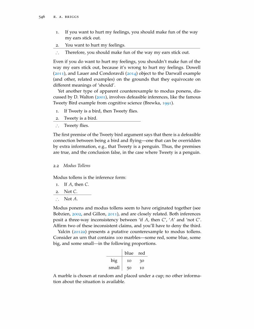
546 r . a . briggs
1. If you want to hurt my feelings, you should make fun of the waymy ears stick out.
2. You want to hurt my feelings.
∴ Therefore, you should make fun of the way my ears stick out.
Even if you do want to hurt my feelings, you shouldn’t make fun of theway my ears stick out, because it’s wrong to hurt my feelings. Dowell(2011), and Lauer and Condoravdi (2014) object to the Darwall example(and other, related examples) on the grounds that they equivocate ondifferent meanings of ‘should’.
Yet another type of apparent counterexample to modus ponens, dis-cussed by D. Walton (2001), involves defeasible inferences, like the famousTweety Bird example from cognitive science (Brewka, 1991).
1. If Tweety is a bird, then Tweety flies.
2. Tweety is a bird.
∴ Tweety flies.
The first premise of the Tweety bird argument says that there is a defeasibleconnection between being a bird and flying—one that can be overriddenby extra information, e.g., that Tweety is a penguin. Thus, the premisesare true, and the conclusion false, in the case where Tweety is a penguin.
2.2 Modus Tollens
Modus tollens is the inference form:1. If A, then C.
2. Not C.
∴ Not A.
Modus ponens and modus tollens seem to have originated together (seeBobzien, 2002, and Gillon, 2011), and are closely related. Both inferencesposit a three-way inconsistency between ‘if A, then C’, ‘A’ and ‘not C’.Affirm two of these inconsistent claims, and you’ll have to deny the third.
Yalcin (2012a) presents a putative counterexample to modus tollens.Consider an urn that contains 100 marbles—some red, some blue, somebig, and some small—in the following proportions.
blue red
big 10 30
small 50 10
A marble is chosen at random and placed under a cup; no other informa-tion about the situation is available.

conditionals 547
In Yalcin’s scenario, it is reasonable to accept the premises, but not theconclusion, of this instance of modus tollens.
1. If the marble is big then it’s likely red.
2. The marble is not likely red.
∴ The marble is not big.
2.3 Conditional Proof
Conditional proof (sometimes called the deduction theorem in formal logic)lets us establish conditional conclusions without relying on any conditionalassumptions. Suppose that an argument from the premises X and A tothe conclusion C is valid. Then conditional proof lets us conclude that theargument from X to ‘if A, then C’ is valid. (Unlike modus ponens andmodus tollens, which let us reason from the truth of some propositions tothe truth of another proposition, conditional proof lets us reason from thevalidity of one argument to the validity of another.)
Stalnaker (1975) gives an argument that can easily be worked into acounterexample to conditional proof (though he does not present it thatway). The following argument is valid, since in classical logic, anythingfollows from a contradiction:
1. The butler did it.
2. The butler didn’t do it.
∴ The gardener did it.
But the following argument is not valid:
1. The butler did it.
∴ If the butler didn’t do it, then the gardener did it.
Although conditional proof in its full generality looks implausible, arestricted version is more appealing: if A all by itself entails C, then ‘if A,then C’ is a truth of logic. (Koons (2014) makes a similar suggestion aboutconditional proof in nonmonotonic logic.)
2.4 Transitivity, Contraposition, and Strengthening the Antecedent
Transitivity is the inference form:
1. If A, then B.
2. If B, then C.
∴ If A, then C.
Contraposition is:

548 r . a . briggs
1. If A, then C.
∴ If not C, then not A.
And strengthening the antecedent is:
1. If A, then C.
∴ If A and B, then C.
All three inference forms seem to fail for ordinary conditionals in En-glish. For transitivity, we have the following counterexample (Stalnaker,1968, p. 106):
1. If J. Edgar Hoover had been born a Russian, then he would havebeen a communist.
2. If J. Edgar Hoover had been a communist, then he would havebeen a traitor.
∴ If J. Edgar Hoover had been born a Russian, then he would havebeen a traitor.
For contraposition, we have the following counterexample (adapted fromAdams, 1988):
1. If it rains, then it does not rain hard.
∴ If it rains hard, then it does not rain.
And for strengthening the antecedent, we have the following counterex-ample (Stalnaker, 1968, p. 106):
1. If this match were struck, then it would light.
∴ Therefore, if this match had been soaked in water overnight and itwere struck, then it would light.
Not everyone accepts these putative counterexamples as genuine. Bro-gaard and Salerno (2008) argue that the meaning of a conditional dependspartly on a contextually determined set of relevant possible worlds. Theyclaim that the putative counterexamples involve a context shift betweenthe premises and the conclusion, but in any fixed context, the argumentsare valid.
Von Fintel (2001), Gillies (2007), and Williams (2008) cite linguistic evi-dence in support of the context shift hypotheses: changing the order ofthe premises and conclusions in the counterexample arguments changeswhether they seem true or false. Counterexamples to antecedent strength-ening are closely related to so-called Sobel sequences (named for Sobel 1970).A Sobel sequence consists of two sentences of the following form (Gillies,2007).
(a) If Sophie had gone to the New York Mets Parade, she would haveseen Pedro Martínez.

conditionals 549
(b) But if Sophie had gone to the New York Mets Parade and gottenstuck behind a tall person, she would not have seen Pedro Martínez.
It seems perfectly reasonable to assert (a) followed by (b). But once some-one has asserted (b), an assertion of (a) seems inappropriate—after all, ifSophie had gone to the parade, who’s to say she would not have gottenstuck behind a tall person?
Fintel, Gillies, and Williams claim that Sobel sequences involve a contextshift: once someone asserts (b), the context changes to make (a) false, but(a) and (b) are never true in the same context. Moss (2012) proposes analternative explanation: once (b) has been asserted, (a) might be true, butis no longer known, since asserting (b) changes the standards a belief mustmeet in order to count as knowledge.
2.5 Simplification of Disjunctive Antecedents
Simplification of disjunctive antecedents (‘simplification’ for short; Nute,1975) is the argument form:
1. If A or B, then C.
∴ If A, then C.
Simplification seems appealing on its face: surely, to say that the bus willbe late if it rains or snows is to say that the bus will be late if it rains, andthe bus will be late if it snows.
However, one can easily generate counterexamples by substituting thesame sentence for B and C. Suppose I have enough money to visit eitherDisneyland or Graceland, but not enough to visit both. Then the premiseof the following argument is true, while its conclusion is false.
1. If I visit Disneyland or I visit Graceland, then I’ll visit Graceland.
∴ If I visit Disneyland, then I’ll visit Graceland.
Counterexamples to strengthening the antecedent can be used to gener-ate counterexamples to simplification (Fine, 1975). Suppose we have bothof the following:
1. If A, then C.
2. Not: if A and B, then C.
A is logically equivalent to [(A and B) or (A and not B)], so by 1, we have:
3. If [(A and B) or (A and not B)], then C.
But by simplification, the truth of 3 would have to entail the falsity of 2.So there is a three-way tension between the validity of simplification,
the invalidity of strengthening the antecedent, and the substitution of

550 r . a . briggs
logical equivalents. All three ways out of the puzzle are representedin the literature: Loewer (1976) and Mckay and Inwagen (1977) rejectsimplification; defenders of strict conditional accounts (Section 4.1) acceptstrengthening the antecedent; and Nute (1975) and Alonso-Ovalle (2009)reject substitution.
3 the indicative/counterfactual distinction
Conditionals in English can be divided into two categories, exemplified bythe following pair of sentences (Adams, 1970):
(DD). If Oswald did not shoot Kennedy, then someone else did.
(HW). If Oswald had not shot Kennedy, then someone else would have.
Although (dd) and (hw) are built up from the same antecedent andconsequent, they mean different things. (dd) would be acceptable to mostpeople familiar with US history: Kennedy was shot, so someone must haveshot him—if not Oswald, then someone else. But (hw) is more contro-versial; it is accepted by conspiracy theorists, but rejected by those whobelieve that Oswald acted alone. Sentences like (dd) are called indicative;sentences like (hw) are called counterfactual (or sometimes subjunctive).
It’s not clear how to classify conditionals whose antecedents concernthe future. Consider the following sentence, as uttered by a conspiratorbefore the Kennedy assassination.
(DW). If Oswald does not shoot Kennedy, then someone else will.
Dudman (1983, 1984) and Bennett (1988) argue that future-tensed condi-tionals like (dw) belong with counterfactuals like (hw); Bennett (2003,2001; yes the same Bennett!) argues that they belong with indicativeslike (dd); Edgington (1995) argues that there exist distinct categories offuture-tensed indicatives and future-tensed counterfactuals.
Philosophers also disagree about the precise relationship between indica-tives and counterfactuals. Some favor what Bennett (2003) calls ‘Y-shapedanalyses’, which first explain what is common to indicatives and counter-factuals, and then bifurcate to explain how this common core can producetwo different kinds of conditionals. Others (notably Gibbard, 1981, andBennett, 2003) argue that we need completely separate theories of in-dicatives and counterfactuals—that there is no interesting core shared byboth.
In what follows, I will write ‘A C’ to indicate a counterfactualconditional; ‘A → C’ to abbreviate an indicative conditional; and ‘if A,then C’ where I wish to remain neutral. I turn now to a popular class oftheories, typically aimed at explaining counterfactual conditionals, butsometimes extended to cover indicatives.

conditionals 551
4 selection functions
One way to give a theory of conditionals is to spell out their truth conditions,i.e., the circumstances under which they are true. Formally, philosophersrepresent the truth conditions of a sentence as a function from possibleworlds (i.e., ways the world might be) to truth values. Fully specifyingthe truth conditions for every conditional would be too tall an order: tounderstand the truth conditions for ‘if ontogeny recapitulates phylogeny,then snakes develop vestigial legs’, we would have to understand the truthconditions of ‘ontogeny recapitulates phylogeny’ and ‘snakes develop ves-tigial legs’, and that job falls outside the scope of a theory of conditionals.So theories of conditionals adopt a more modest aim: to give a recipe forderiving the truth conditions for ‘if A, then C’ from the truth conditionsof (arbitrary) A and C.
The concept of a selection function (Stalnaker, 1968) provides a way ofassigning truth conditions to a conditional based on the truth conditionsof its antecedent and consequent. The basic idea is that, to evaluate ‘if A,then C’, we should first consider a set of selected possible worlds where Ais true. (Henceforth, I will use ‘A-worlds’ as shorthand for ‘worlds whereA is true’.) Intuitively, the selected worlds represent ways the actual worldmight be if A were true. We then check whether, at all the selected worlds,C is true. If so, then the counterfactual conditional ‘if A, then C’ is true atthe actual world; otherwise, it is false at the actual world.
More formally, we can model this process in terms of a selection functionf that maps ordered pairs consisting of a possible world and a propositiononto sets of possible worlds. ‘If A, then C’ is true at a possible worldw if and only if C is true at every world in f (A, w). Different ways ofinterpreting the selection function yield different theories of conditionals.
4.1 Strict Conditionals
One natural way to interpret the selection function is to check all possibleA-worlds, and say that ‘if A, then C’ is true at world w just in case C istrue at all of them. (Since what is possible may depend on what is actual,the truth value of the conditional may vary from world to world.) Thisapproach yields the strict conditional interpretation of the selection function,first developed by C. Lewis (1918). The strict conditional approach classifiestransitivity, contraposition, and antecedent-strengthening as valid—whichits opponents claim is a mistake (see D. Lewis, 1973a, pp. 4–12).
The strict conditional interpretation also gives questionable results aboutwhich counterfactuals are true. If I were to leap out of the second-storywindow of my office, I would hurt myself—but the strict conditionalaccount says this is not so. There are possible worlds where I leap out the

552 r . a . briggs
second-story window and remain unharmed: some where there is a safetynet underneath the window, some where I am thoroughly ensconcedin protective bubble wrap, some where my body is much less fragilethan ordinary human bodies, some where the Earth’s gravitational fieldis weak. . . but none of them is the sort of world that would result, ifI were to leap out the second-story window. Hájek (manuscript) sumsup the problem this way: on the strict conditional interpretation, mostcounterfactuals are false.2
4.2 Closest Worlds
An alternative to the strict conditional approach, typically used for coun-terfactuals, defines the selection function in terms of similarity amongpossible worlds. For every world w, we can rank worlds from most similarto w (‘closest’) to least similar (‘farthest away’). D. Lewis (1973a) holds thatevery such ranking is a total preorder: two worlds can be equally similar tow, but they must be comparable, so that either they are equally similar orone is more similar than the other. (Stalnaker, 1968, discusses the specialcase of the logic where no two worlds are equally close to a given world;Pollock, 1976, discusses a generalization where worlds may be incompara-ble in terms of closeness.) A C is true at w just in case C is true at allthe A-worlds that are most similar to w.
Formally, the closest-worlds interpretation can be modeled using asystem of ‘spheres’—sets of worlds such that every world in the set iscloser to w than every world outside it (D. Lewis, 1973a). Then f (A, w) isthe intersection of the set of A-worlds with the smallest sphere containingat least one A-world.3
Unlike the strict conditional interpretation, the closest-worlds interpreta-tion of the selection function can explain why transitivity, contraposition,and antecedent-strengthening seem invalid. On the closest-worlds inter-pretation, they are invalid, and we can use diagrams (adapted from D.Lewis, 1973a) to illustrate why.
To see why transitivity is invalid, consider a system of spheres modelcentered on a particular world w, depicted in Figure 1a. (Worlds are pointsin the diagram, and spheres are concentric circles.) The A-worlds arethe points inside the shape labeled A, the B-worlds are the points inside
2 Hájek argues that the problem extends beyond strict conditional accounts; it also affectsthe closest-worlds account in Section 4.2. K. S. Lewis (2015) argues that we can save theclosest-worlds account by ignoring worlds that are deemed irrelevant by a contextually-determined standard of relevance.
3 Some technical difficulties arise when there is no smallest sphere containing at leastone A-world, but only a limitless sequence of ever-smaller spheres; see D. Lewis (1973b,pp. 424–425); Stalnaker (1981, pp. 96–99); Warmbrod (1982); and Díez (2015) for discussion.

conditionals 553
the shape labeled B, and the C-worlds are the points inside the shapelabeled C. All the closest A-worlds to w are B-worlds, and all the closestB-worlds are C-worlds; yet none of the closest A-worlds are C-worlds.Figure 1b shows a counterexample to contraposition, and Figure 1c showsa counterexample to antecedent strengthening.
Defenders of the closest-worlds theory have the burden of spelling outwhat ‘closeness’ amounts to. D. Lewis (1973a) claims that closeness isbased on similarity among worlds: to say that one world is closer to wthan another is to say that the first world is more similar to w than thesecond. But Fine (1975) presents an example where greater similarity doesnot make for greater closeness. (I have taken a few liberties with the detailsof the example.)
On September 26, 1983, at the height of the Cold War, a Soviet early-warning system went off, falsely reporting that missiles had been launchedat Russia from the US (Aksenov, 2013). The officer who saw the alarm,Stanislav Petrov, did not report it to his superiors, and so Russia did notlaunch missiles in retaliation. The following conditional seems true:
PETROV. If Petrov had informed his superiors at the time of the falsealarm, then there would have been a nuclear war.
After all, Petrov’s superiors were poised to launch the missiles in the eventof an attack, and it seems that the phone lines and missile system were inworking order. The only missing ingredient was the report from Petrov.
But among the worlds where Petrov informs his superiors at the timeof the false alarm, those where the Soviet missile launch is preventedby a happy accident—incompetence by Petrov’s superiors, or a brokentelephone, or a malfunction of the Soviet missile system—are more similarto the actual world than those where the launch goes through. Worldswhere the missile launch is prevented by a happy accident agree with theactual world about the total number of nuclear wars in the 20th Century—surely a more important dimension of similarity than the functioning ormalfunctioning of one measly telephone line.4
4.3 Past Predominance
To handle the petrov example, a natural thought goes, we need an accountof the selection function that treats the past differently from the future.When Petrov made his choice, the missile launch system was already in
4 Defenders of the closest-worlds interpretation reply that we should understand ‘similarity’so that agreeing about the total number of nuclear wars in the 20th Century does not makefor greater similarity than agreeing about the functioning or malfunctioning of one measlytelephone line; see D. Lewis (1979) and Arregui (2009).

554 r . a . briggs
w
A
BC
(a) Transitivity
w
A
B
(b) Contraposition
w
B
AC
(c) Strengthening the antecedent
Figure 1: Counterexamples to transitivity, contraposition, and strengthening theantecedent in the closest-worlds framework

conditionals 555
t1
t3 t6 t9
t2
t5 t8
t4 t7
Figure 2: A model of branching time
working order—but it was not yet determined whether there would be awar.
Thomason and Gupta (1980) propose an account of the selection functionthat takes seriously the past-future asymmetry. They model the universeusing branching time, where each moment has only one possible past,but multiple possible futures. (Cross, 1990, shows that the assumption ofbranching time is dispensable; past predominance can also be modeledusing ordinary possible worlds.) Figure 2 depicts such a model. Thenodes t1, t2, . . . , t9 are moments. Paths through the tree—in this example,t1, t2, t4, t7, t1, t2, t5, t8, and t1, t3, t6, t9—are called histories.
We can think of each possible world as containing information aboutwhich moment is present, as well as information about which history isactual. (On this way of understanding the model, even when the presentmoment has more than one possible future, there is a fact of the matterabout which future will occur.)
Thomason and Gupta adopt a past predominance principle, which saysthat if a world is in f (A, w), then it must diverge from w as late aspossible—there can be no other A-world whose history overlaps w for alonger span than f (A, w).5
The past predominance view can explain the petrov example. Con-sider the following interpretation of our diagram: the actual history ist1, t2, t4, t7. At t1, it is not yet settled whether the early warning systemgoes off. The early warning system goes off t2, and Petrov must decidewhat to do. (At t3, which belongs to an alternative history, there is neverany alarm.) At t4, Petrov decides not to notify his superiors, and so att7, there is no nuclear war. (At t5, which belongs to another alternativehistory, Petrov decides to notify his superiors, and a nuclear war ensues att8.)
Now consider the conditional petrov, as uttered at t7. Its antecedent isfalse at the actual world, which has the history t1, t2, t4, t7. The closest
5 For technical reasons, Thomason and Gupta also assume that f (A, w) is a singleton set,and posit that each world contains a choice function, which specifies not just what the futurewill be like, but what the future would have been like had the past gone differently. I passover the details.

556 r . a . briggs
worlds where its antecedent is true must have the history t1, t2, t5, t8,which diverges from the actual world’s history at the last possible momentyet still makes the antecedent true. Since the actual present moment is t7,it seems reasonable to select t8 as the present moment at all the closestworlds. Since there is a nuclear war at t8, the consequent of petrov is trueat all the the closest worlds; hence petrov is true at the actual world.
4.4 Causal Models
A class of examples called Morgenbesser cases (Slote, 1978, 27n) suggest thatthe selection function should respect causal as well as temporal constraints.Edgington (2004) gives a representative Morgenbesser case.
Our heroine misses a flight to Paris due to a car breakdown. She com-plains to the repairman: ‘If I had caught the plane, I would have beenhalfway to Paris by now!’ But he corrects her: ‘I was listening to the radio.It crashed. If you had caught that plane, you would be dead by now.’
The repairman claims that the following counterfactual is true.
LETHAL. If the heroine had caught that plane, she would be dead bynow.
He is right. It’s not clear that past predominance can explain why he’sright: the plane crash occurs after our heroine would have made herflight.6 What matters is that the plane crash is causally independent ofwhether she makes her flight. This is why, when assessing what wouldhave happened if our heroine had made her flight, we should hold theplane crash fixed.
Pearl (2009) proposes a causal theory of counterfactuals that accountsfor Morgenbesser cases. His theory relies on the concept of a causal model,consisting of a set of variables, which represent what circumscribed partsof the world are like, and a set of structural equations, which representdirect causal links between variables. Each variable is assigned an actualvalue; we can think of variables as questions about parts of the world, theirpossible values as possible answers to those questions, and their actualvalues as the correct answers in the actual world. Note that although Iintroduced selection semantics as a recipe for assigning truth values toconditionals at worlds, Pearl’s theory is a recipe for assigning truth valuesto conditionals at model-valuation pairs.7
6 But see Phillips (2007) for an argument that past predominance can provide an adequateexplanation.
7 Pearl’s theory can be understood as a version of the situation semantics defended byBarwise and Perry (1981). Instead of assigning truth values to propositions at worlds, itassigns truth values to propositions at situations, which represent ways that circumscribedparts of the world could be.
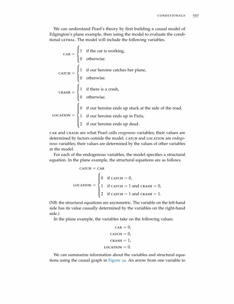
conditionals 557
We can understand Pearl’s theory by first building a causal model ofEdgington’s plane example, then using the model to evaluate the condi-tional lethal. The model will include the following variables.
car =
1 if the car is working,
0 otherwise.
catch =
1 if our heroine catches her plane,
0 otherwise.
crash =
1 if there is a crash,
0 otherwise.
location =
0 if our heroine ends up stuck at the side of the road,
1 if our heroine ends up in Paris,
2 if our heroine ends up dead.
car and crash are what Pearl calls exogenous variables; their values aredetermined by factors outside the model. catch and location are endoge-nous variables; their values are determined by the values of other variablesin the model.
For each of the endogenous variables, the model specifies a structuralequation. In the plane example, the structural equations are as follows.
catch = car
location =
0 if catch = 0,
1 if catch = 1 and crash = 0,
2 if catch = 1 and crash = 1.
(NB: the structural equations are asymmetric. The variable on the left-handside has its value causally determined by the variables on the right-handside.)
In the plane example, the variables take on the following values.
car = 0,
catch = 0,
crash = 1,
location = 0.
We can summarize information about the variables and structural equa-tions using the causal graph in Figure 3a. An arrow from one variable to

558 r . a . briggs
car catch
crash location
(a) The actual model
car catch
crash location
(b) The submodel generated by intervening to make the antecedent true
Figure 3: Causal graph used to evaluate the counterfactual lethal: ‘If the heroinehad caught that plane, she would be dead by now’.
another indicates that the first variable exerts direct causal influence onthe second, but unlike the structural equations, the causal graph doesn’tspecify the nature of that influence.
Given a pair consisting of a model and an assignment of values tovariables in the model, we can use a selection function to assign truthvalues to conditionals. (This time, the selection function takes in a model,and returns a singleton containing one new model.) Pearl’s account isrestricted to counterfactuals whose antecedents are either ‘literals’, whichsay that a particular variable takes on a particular value, or conjunctionsof literals. (So ‘the heroine’s car breaks down and the plane crashes’ is anacceptable antecedent, while ‘the heroine’s car breaks down or the planecrashes’ is not.)
Where 〈M, V〉 is a model paired with an assignment of values to vari-ables, and A is an antecedent with the appropriate form, we can generate asubmodel 〈MA, VA〉 by ‘intervening’ on 〈M, V〉 to make A true. Intuitively,we can imagine an intervention as an action by someone outside the modelwho ‘reaches in’ to make the antecedent true, without tinkering withvariables that are causally independent of the antecedent. For instance,a cabbie could intervene to set catch = 1 by driving our heroine to theairport regardless of whether or not her car has broken down.
Formally, the submodel MA is a model with the same variables as M,but different structural equations. If X is one of the variables mentioned in

conditionals 559
A, and X is endogenous, we delete the structural equation correspondingto X, and make X exogenous instead. (This corresponds to the idea that anintervention makes A true regardless of whether its typical causes obtain;the intervening cabbie enables the heroine to get to the airport whetheror not her car is in working order.) We then set the value VA of eachX mentioned in A to the value specified by A. (This corresponds to theidea that the intervention makes the antecedent true.) If a variable is notcausally influenced (either directly or indirectly) by any of the variablesmentioned in the antecedent, then VA assigns it the same value as V. (Thiscorresponds to the idea that an intervention is minimal, so that only thevariables mentioned in the antecedent are directly affected.) Finally, if avariable is causally influenced by one of the variables mentioned in theantecedent, then its value VA is fixed by the structural equations. (Thiscorresponds to the idea that an intervention is minimal in another sense: itdoes not interfere with the downstream effects of the variables mentionedin the antecedent.)
We are now ready to evaluate the counterfactual
LETHAL. If the heroine had caught that plane, she would be dead bynow.
in our original model. To check whether lethal is true in the originalmodel, we intervene to make its antecedent true—i.e., to set catch = 1.We then check whether the consequent is true (i.e., location = 2) in theresulting submodel.
First, we delete the structural equation for catch, turning catch intoan exogenous variable. Our only remaining structural equation is
location =
0 if catch = 0,
1 if catch = 1 and crash = 0,
2 if catch = 1 and crash = 1.
(The graph for the resulting submodel is shown in Figure 3b.)Second, we set the values of the variables. The antecedent requires that
catch = 1.
Since neither car nor crash is downstream from catch, we have
car = 0,
crash = 1.
Finally, the value of location is fixed by the structural equation. Sincecatch = 1 and crash = 1, we have
location = 2.

560 r . a . briggs
Therefore, in the submodel, the protagonist is dead, so in the originalmodel, had she caught her plane, she would have been dead.
The procedure described is a type of selection semantics: given anantecedent and a model-valuation pair, we call on a ‘submodel’ selectionfunction that returns the singleton set of another model-valuation pair(a submodel). Galles and Pearl (1998) argue that this selection semanticsis formally equivalent to the closest-worlds account. However, there isa key difference between the two accounts: the selection semantics letsus assigns truth conditions to counterfactuals built up from arbitrarysentences, while the causal modeling account only lets us assign truthvalues to counterfactuals whose antecedents are literals, or conjunctionsof literals. Schulz (2011) and Briggs (2012) propose ways of extendingthe language to counterfactuals with logically complex antecedents; theirproposed theories are logically inequivalent to the closest-worlds semantics.Huber (2013) proposes an alternative way of extending the language thatmakes it logically equivalent to the closest-worlds account.
5 counterpossible conditionals
Selection semantics has trouble with counterpossible conditionals—that is,conditionals whose antecedents are impossible. It counts all counterpos-sible conditionals as trivially true. Where A is impossible, there are nopossible A-worlds. Therefore, if we feed the selection function an impos-sibility A and a world w and ask it to return a set of possible A-worlds,it returns the empty set. Trivially, all the A-worlds in the empty set areC-worlds, so that trivially A C is true in the original world.
But counterpossibles seem to have non-trivial truth conditions: someare true, while others are false. Examples of true counterpossibles include:
If Hobbes had (secretly) squared the circle, sick children in themountains of South America at the time would not have cared(Nolan, 1997, p. 544).
If I were a horse, then I would have hooves (Krakauer, 2012, p. 10).
If wishes were horses, beggars would ride (Krakauer, 2012, p. 10).
If intuitionistic logic were the correct logic, then the law of excludedmiddle would no longer be unrestrictedly valid (adapted from Bro-gaard & Salerno, 2013).
Corresponding examples of false counterpossibles include:
If Hobbes had (secretly) squared the circle, sick children in themountains of South America at the time would have taken notice.

conditionals 561
If I were a horse, then I would have scales.
If wishes were horses, no one would own any horses.
If intuitionistic logic were the correct logic, then the law of excludedmiddle would still be unrestrictedly valid.
Assigning non-trivial truth values to counterpossibles doesn’t just cap-ture linguistic intuitions; it also enables counterpossibles to do valuablephilosophical work. Non-trivial counterpossibles help us assess rival philo-sophical, mathematical, and logical theories by telling us what wouldfollow if those theories were true (Krakauer, 2012; Brogaard & Salerno,2013; Nolan, 1997). They explain how necessary events and omissions ofimpossible events are causally relevant to the actual world—how a mathe-matician’s failure to disprove Fermat’s Last Theorem prevented her fromgetting tenure, how my failure to be in two places at once caused me tomiss a colloquium talk, or how the copresence of a mental property and itssubvening physical property can result in a subject’s raising his arm (Bern-stein, 2016). They can be used to give an account of essences: an essentialproperty is one such that, if the bearer had lacked it, then the bearer wouldnot have existed (Brogaard & Salerno, 2013, 2007). (Non-trivial counterpos-sibles save this account from certain implausible commitments—e.g., thatliving in a world where 2 + 2 = 4 is trivially part of everyone’s essence.)
Not everybody agrees that counterpossibles have non-trivial truth values,however. Williamson (2007, p. 172) argues that apparent examples of non-trivial counterpossibles collapse under closer scrutiny. In a slight varianton Williamson’s example,8 imagine that a student is mulling over a gradedarithmetic test. Of the 12 problems on the test, the student has gottenthe last one wrong: ‘what is 5 + 7?’ The student, who answered ‘11’,laments: ‘If only 5 + 7 were 11, I would have gotten a perfect score!’ Thisseems to be true, and furthermore, it seems false that if 5 + 7 were 11, thestudent would have gotten one of the problems wrong. But appearancesare deceptive. Suppose that 5 + 7 were 11. Then in answering all theproblems right, the student would have given five right answers followedby seven more right answers, for a total of 11 right answers. Since thereare 12 problems on the test, the student would have gotten one problemwrong after all. (For a rebuttal of Williamson’s argument, see Salerno andBrogaard, 2007.)
5.1 Impossible Worlds
Nolan (1997) gives an account of counterpossibles by supplementing theclosest-worlds account with impossible worlds—ways the world couldn’t
8 Thanks to Sharon Berry for suggesting this version in conversation.

562 r . a . briggs
be. We can then say that A B is true at w just in case B is true at allthe closest possible or impossible A-worlds to w. Two questions then arise:what are impossible worlds, and what makes them closer to or furtheraway from the actual world?
The ontology of impossible worlds has spawned its own literature: theymay be collections of individuals like our actual world (Yagisawa, 2010),or they may be sets of sentences in some suitable language (Hintikka,1975; Melia, 2001; Sider, 2002; see Berto, 2013, for a general overview anddiscussion.) Another pressing question for theorists of counterpossiblesconcerns the logical structure of impossible worlds. Is it the case that forevery set of sentences, there is some impossible world where all and onlythe sentences in the set are true? Or is there more logical structure we canimpose on impossible worlds?
Proponents of impossible worlds typically don’t require that the im-possible worlds be closed under classical logical consequence—in otherwords, they don’t require that whenever some propositions are true at animpossible world, all the classical logical consequences of those propo-sitions are true at the world too. If impossible worlds had to be closedunder classical logical consequence, then whenever A was impossible bythe rules of classical logic, A C would be trivially true. Nolan (1997,p. 547) argues that we should not require impossible worlds to be closedunder any kind of logical consequence, since for every putative logicaltruth, there are non-trivial facts about what the world would be like ifthat logical truth did not obtain. A similar line of reasoning suggests thatsome impossible worlds have truth-value gluts: we can speculate aboutwhat would happen if there were true contradictions, so there must beimpossible worlds at which there are true contradictions.
Bjerring (2013) argues that some impossible worlds have truth-valuegaps. Otherwise, he argues, our theory of counterpossibles would misclas-sify certain conditionals as true, such as this one: ‘If intuitionistic logicwere correct, then the Law of Excluded Middle would hold.’ (The Law ofExcluded Middle says of every proposition that either it or its negationholds; intuitionists famously deny it.)
What about closeness? Nolan (1997) proposes the
Strangeness of Impossibility Condition. Any possible world is moresimilar [closer] to the actual world than any impossible world (Nolan,1997, p. 550).
The Strangeness of Impossibility Condition ensures that where A is apossible proposition, supplementing the closest-worlds account with im-possible worlds has no effect on how we evaluate A C. So long as Ais possible, the set of closest possible A-worlds coincides with the set ofclosest possible or impossible A-worlds.

conditionals 563
Bjerring (2013, p. 348) proposes another constraint on closeness, whichimplicitly relativizes closeness to the antecedent of a counterfactual. Givena collection of logical systems L1, L2, . . . , Ln, where L1 is classical logic, andwhere WLi is the set of worlds deductively closed under Li’s entailmentrelation, Bjerring endorses the
Relative Closeness Condition. For any counterfactual whose antece-dent presupposes that some logic Li is correct (true, adequate), aworld in modal space WLi is closer to the actual world than anyworld in modal space WLj , where WLi 6= WLj , and where i ≥ 1 andj > 1.9
Brogaard and Salerno (2013) develop a theory on which impossibleworlds are close to the actual world to the extent that they
1. minimize discrepancies with relevant background facts about theactual world (where the relevance of background facts is fixed bycontext), and
2. minimize violations of relevant a priori entailment (where relevant apriori entailment is spelled out in more detail in the paper).
As an illustration of these conditions, Brogaard and Salerno use them toevaluate the counterpossible conditional ‘if water had not been H2O, thenwater would have been a monkey’. This counterpossible is false. Theirtheory delivers the correct verdict, they claim, because it is a priori thatwater is not a monkey.
To derive this verdict, they consider two impossible worlds where the an-tecedent is true. At w1, water is some chemical compound XYZ (differentfrom H2O), while at w2, water is a monkey.
w1 w2
water is not H2O water is not H2O
water is XYZ water is a monkey
Since there are more a priori truths that hold at w1 than at w2, and sinceboth agree with the actual world about the same number of propositions,w1 is closer to the actual world than w2. (Brogaard and Salerno tacitlyassume that there are no antecedent worlds closer to the actual world than
9 As stated by Bjerring, the Relative Closeness Condition seems to presuppose that WLi andWLj do not intersect. We can get rid of this presupposition by modifying the conditionslightly:
Relative Closeness Condition∗. For any counterfactual whose antecedent presupposes
that some logic Li is correct (true, adequate), a world in modal space WLi is closer tothe actual world than any world outside WLi .

564 r . a . briggs
w1 or w2.) Thus, at least one of the closest impossible worlds where wateris not H2O is one where water fails to be a monkey, so the conditional isfalse at the actual world.
5.2 Relevant Logic
Relevant logics are motivated by the thought that the conditional ‘if A,then C’ claims that the truth of A is connected to the truth of C. Relevantlogics originated as rivals to the material conditional account, on whichthe conditional ‘if A, then C’ is true just in case A is false or C is true (seeSection 6). However, some of the same intuitions that favor relevant logicsover the material conditional account also favor them over the closest-worlds account. After all, the reason it seems wrong to say ‘if Hobbes hadsquared the circle, sick children in the mountains of South America wouldhave cared’ is that there is no connection between Hobbes’s squaring thecircle and the interests of sick South American children. Likewise, thereason it seems right to say ‘if I were a horse, I would have hooves’ isbecause something’s being a horse is connected to its having hooves.
Relevant logics are often characterized in proof-theoretic terms. ButRoutley and Meyer (1973, 1972a, 1972b) develop a versatile semantics forthe conditionals of relevant logics, which generalizes the strict conditionalsemantics of Section 4.1. Recall that on the strict conditional interpretation,A C is true at w just in case C is true at all possible A-worlds (relativeto w). We can rewrite the selection function in terms of a two-place ac-cessibility relation among worlds: we say that Rwx just in case world x ispossible according to world w, and that f (A, w) is the set of all A-worldsx such that Rwx.
Routley and Meyer interpret the conditional in terms of a three-placeaccessibility relation among worlds. ‘If A, then C’ is true at w just in case,for all worlds x and y such that Rwxy and x is an A world, C is true at y.Different restrictions on relation R generate different relevant logics. (Forsome logics, we need impossible worlds where both a sentence and itsnegation fail to be true, or impossible worlds where both sentence and itsnegation are true.)
This three-place R relation is formally useful, but does it mean anything?Beall et al. (2012) propose three interpretations of Rwxy, which springfrom different ways of grouping w, x, and y.10 All three interpretationscan be illustrated with the conditional
THERMITE. If you light a bucket of thermite with a titanium fuse, then ahuge explosion will ensue.
10 For a discussion of other ways of interpreting the ternary relation, with references, seeJago (2013).

conditionals 565
grouping the second and third worlds together : Rw〈xy〉 .‘If A, then C’ says at the actual world w, there are no counterexampleswhere A is true and C is false. We typically think of counterexamples asinvolving a single world which makes some things true and other thingsfalse, but relevant logicians split the labor between two worlds x and y, sothat whatever holds at x is true, while whatever fails to hold at y is false.In the example of thermite, we might think of potential counterexamplesas divided into an earlier part x, when a bucket of thermite may or maynot be lit with a titanium fuse, and a later part y, when there may or maynot be an explosion. If the actual world w admits some possible two-partscenarios that begin with the lighting of thermite with a titanium fuse, butfails to end in a huge explosion, then these scenarios are counterexamplesthat falsify thermite.
grouping the first and second worlds together : R〈wx〉y .‘If A, then C’ says that using one’s current information to draw inferencesfrom A will yield the information that C. To say that Rwxy is to say thatwhen the rules of w are applied to the information in x, it is possible toinfer y (or some information that entails y). In the case of thermite, wecan imagine w as a parcel of information specifying the actual laws ofnature, and x as another parcel of information specifying that a bucketof thermite has been lit with a titanium fuse. If sticking these parcels ofinformation together licenses the conclusion that there has been a hugeexplosion (and does so no matter how we fill in x, the information thatthe thermite has been lit), then the conditional thermite is true.
grouping the first and third worlds together : Rw〉x〈y . ‘IfA, then C’ says that C is necessary relative to A, or that C is necessaryin an A-ish way. The conditional thermite does not say it is absolutelynecessary that a huge explosion will ensue. The world w may permit apossible scenario y in which no huge explosions occur. However, once weenrich w with some additional information x, specifying that a bucket ofthermite has been lit with a titanium fuse, we can consider what is possibleunder that supposition. If there is some way of filling in the antecedentthat makes y a possibility, then y is possible not just absolutely, but underthe supposition that the antecedent of thermite is true.
Mares and Fuhrmann (1995) propose a theory of counterfactuals thatcombines the closest-worlds interpretation of the selection function withthe relevant interpretation of the conditional: A B is true at a world wjust in case the relevant conditional ‘if A, then B’ is true at all closest A-worlds to w. Mares (1994) argues that this theory has useful applications toconditional analyses of causation, and to theories of conditional obligation.

566 r . a . briggs
6 the material conditional account of indicatives
According to the material conditional account defended by Grice (1989)and Jackson (1987), an indicative conditional A → C is true just in caseeither its antecedent A is true, or its consequent C is false. (The materialconditional account is almost always offered as a theory of indicative condi-tionals alone, since counterfactual conditionals with false antecedents canbe false. Even though I don’t keep a horse, it is false that if I were to keep ahorse, it would breathe fire.) The material conditional account has a simpleexplanation for the apparent validity of all the the inferences discussed inSection 2 (modus ponens, modus tollens, conditional proof, strengthen-ing the antecedent, transitivity, contraposition, and simplification): theseinferences really are valid.
Furthermore, there are persuasive arguments for the conclusion thatan indicative conditional A→ C is true if and only if the correspondingmaterial conditional ‘not A or C’ is true. Suppose the indicative conditionalis true. Then it can’t have a true antecedent and a false consequent; thatwould be a violation of modus ponens. So the indicative conditionalentails the material conditional. But when I know that either C holds or Adoesn’t, I can infer that if A, then C. So the material conditional entails theindicative. (Stalnaker, 1975, p. 136, calls this the direct argument.) Sincethe material and indicative conditionals entail each other, they must beequivalent.
Gibbard (1981) provides a formal argument for the equivalence of theindicative and material conditionals based on three logical principles.Where ‘not A’ is abbreviated ¬A and ‘A or B’ is abbreviated A ∨ B, theprinciples are:
Pseudo Modus Ponens. A→ C entails ¬A ∨ C.
Import-Export. A→ (B→ C) is equivalent to (A ∧ B)→ C.
Conditional Proof. If A entails C, then A→ C is a logical truth.
To show that A → C and ¬A ∨ C are equivalent, Gibbard only needs toshow that each entails the other. By Pseudo Modus Ponens, A→ C entails¬A ∨ C. The proof that ¬A ∨ C entails A→ C is as follows.
1. ((¬A ∨ C) ∧ A) entails C. (By tautological reasoning.)
2. It is a truth of logic that ((¬A ∨ C) ∧ A)→ C. (By 1 and ConditionalProof.)
3. It is a truth of logic that (¬A ∨ C) → (A → C). (By 2 and Import-Export.)

conditionals 567
4. It is a truth of logic that ¬(¬A ∨ C) ∨ (A → C). (By 3 and PseudoModus Ponens.)
5. (¬A ∨ C) entails (A→ C). (By 4 and tautological reasoning.)
Despite these points in its favor, the material conditional account facessubstantial difficulties. It seems to yield wrong predictions about logicalvalidity, often called ‘paradoxes of material implication’.
For example,the material conditional account entails that all of thefollowing are truths of logic:
Either the unburied dead will walk the Earth if I bury a chicken headin my backyard, or the unburied dead will walk the Earth if I fail tobury a chicken head in my backyard (McGee, 2005).
Either you are virtuous if you are rich, or you are rich if you arevirtuous.
One of these three things holds: if you grant voting rights to children,you will grant them to guinea pigs; if you grant voting rights toguinea pigs, you will grant them to inanimate objects; or if you grantvoting rights to inanimate objects, you will take them away fromadult human beings.
Furthermore, the material conditional account entails that all of the follow-ing inferences are valid. (The proof of God’s existence is due to Edgington,1986.)
1. I will not do my chores today.
∴ If I do my chores today, then the world will implode.
1. Dinner will be delicious.
∴ If I burn the veggie burgers and pour sand into the sweet potatoes,then dinner will be delicious.
1. If God does not exist, then it’s not the case that if I pray, my prayerswill be answered.
2. I do not pray.
∴ God exists.
In addition to yielding bad predictions about validity, the materialconditional account yields bad predictions about the probabilities of con-ditionals. Suppose I draw a card at random from a 52-card deck. Thematerial conditional ‘either I do not draw a red ace, or I draw the ace ofhearts’ has probability 51/52. (The only way for me to make it false is todraw the ace of diamonds.) Therefore, by the material conditional account,I should assign probability 51/52 to the indicative conditional ‘if I draw a
568 r . a . briggs
red ace, then it will be the ace of hearts’. But the indicative conditional ‘ifI draw a red ace, then it will be the ace of hearts’ should get probability1/2, since half the time when I draw a red ace, it will be an ace of hearts.
More generally, the material conditional account falls afoul of
The Thesis. Whenever A and C are propositions, the probability of theindicative conditional A→ C is equal to the conditional probabilityof C given A, understood as
Pr(A|C) = Pr(A ∧ C)Pr(C)
.
the thesis is a plausible way of unpacking the so-called Ramsey test, basedon a famous remark by Ramsey (1978, 143n):
If two people are arguing ‘If p will q?’; and are both in doubtas to p, they are adding p hypothetically to their stock ofknowledge and arguing on that basis about q; so that in a sense‘If p, q’ and ‘If p, [not q]’ are contradictories.
Unfortunately, the material conditional account is straightforwardly in-compatible with the thesis, and with the Ramsey test more generally. Theprobability that a material conditional is true is not, in general, the condi-tional probability of the consequent given the antecedent. (The probabilityof the material conditional may be anywhere between that conditionalprobability and 1.) Furthermore, where A is highly unlikely, the materialconditional ‘not A or C’ is both highly believable and highly assertible,whether or not adding A to one’s stock of knowledge would justify a highdegree of confidence in C.
Grice (1989) and Jackson (1987) explain these wrong predictions bydistinguishing between true sentences and sentences that can appropriatelybe asserted. According to Grice, in a situation where I will not do mychores today, it is technically true that if I do my chores today, then theworld will implode. Likewise, in a situation where dinner will be delicious,it is technically true that if I burn the veggie burgers and pour sand into thesweet potatoes, then dinner will be delicious. Nonetheless, it is misleadingto assert a conditional when I know that its antecedent is false, or when Iknow that its consequent is true, because it is misleading to assert a weakclaim when I could have asserted a stronger one. Refusing to assert thestronger claim is liable to mislead my audience into thinking that I donot know it. The supposedly paradoxical arguments are valid. When theirpremises are true, their conclusions may be bad, but this does not maketheir conclusions false.
Grice’s proposed mechanism for explaining away the problem is usefulin other domains: it can explain why some non-conditional assertions are

conditionals 569
misleading. For instance, if you ask where John is, and I know that heis in the library, it is misleading for me to reply ‘He is either at the pub,or in the library.’ A similar trick works for negated conjunctions, as anexample by D. Lewis (1976) shows. If I point out a harmless mushroomthat I plan to keep for myself, and remark ‘You won’t eat that and live’,knowing that my assertion will prevent you from eating it, then I am guiltyof misleading you, though what I say is technically true.
Jackson (1987) is not satisfied with Grice’s explanation, since sometimes,it is all right to assert an indicative conditional even if you know that theantecedent is false, or the consequent is true. I know that Oswald killedKennedy, but can nonetheless assert that if Oswald didn’t kill Kennedy,someone else did. Jackson has a different explanation for why technicallytrue conditionals might sound wrong. While the material conditionalaccount captures the truth conditions of an indicative conditional, themeaning of ‘if. . . then. . . ’ goes beyond its truth conditions. Built into themeaning of an English indicative conditional is the implication that itwould still be appropriate to assert the material conditional, even if itsantecedent were known. (Jackson calls this feature ‘robustness’.) TheOswald-Kennedy conditional is robust, because even if I had reason todoubt that Oswald killed Kennedy, I would still have good reasons tobelieve that either Oswald or someone else killed him.
7 the no truth values (ntv) account of indicatives
Suppose you are convinced that the material conditional account gives thewrong truth conditions for the indicative conditionals. You might hopethat there was some other account of the truth conditions for indicativeconditionals—one that could better explain the truth of the thesis. Un-fortunately, a collection of so-called ‘triviality theorems’ suggests that notruth conditions whatsoever will do the trick. Triviality theorems motivateEdgington (1986, 1995) and Appiah (1985) to claim that indicative condi-tionals lack truth values altogether. (Edgington, 2008, goes on to developa Y-shaped theory on which counterfactual conditionals also lack truthvalues altogether.)
In general, triviality theorems show that if the thesis is true in general,then every probability function is trivial: it assigns positive probabilityto at most two mutually exclusive alternatives. But it is absurd to claimthat every probability function is trivial. (Here is a non-trivial probabilityfunction: the one that assigns probability 1/6 to each possible outcome ofthe roll of a single die.) Therefore, we must reject the thesis.
To see how triviality theorems work, we can consider an early result byD. Lewis (1976), illustrated by system of diagrams adapted from Edgington(1995). Edgington visualizes probabilities using rectangles, divided into

570 r . a . briggs
C
¬C
A
¬A
A
¬A
Figure 4: A probability space
horizontal segments representing propositions. The height of a segmentrepresents the probability of the corresponding proposition; the entirerectangle is normalized to have height 1. In Figure 4 the proposition C hasprobability 1/2. C is subdivided into the propositions A ∧ C (probability1/4) and A ∧ ¬C (probability 1/4). ¬C (also with probability 1/2) issubdivided into the propositions ¬C ∧ A (probability 1/8) and ¬C ∧ ¬A(probability 3/8).
Figure 5 shows how to calculate the probability of A conditional on C byerasing the bottom half of the diagram, and stretching out the remainingpart of the rectangle so its height is 1 (in effect multiplying the heightof each of its sub-regions by 1
Pr(C) ). The new height of the A region isPr(A|C).
According to the Law of Total Probability (illustrated in Figure 6), forany two propositions X and Y,
Pr(Y) = Pr(Y|X)× Pr(X) + Pr(Y|¬X)× Pr(¬X). (1)
Consider any two propositions A and C such that P(A ∧ C) > 0, andP(A ∧ ¬C) > 0. Plugging in A for X and A → C for Y in Equation 1
yields:
Pr(A→ C) = Pr(A→ C|C)× Pr(C) + Pr(A→ C|¬C)× Pr(¬C). (2)
In other words, we can split the probability space into a C part anda ¬C part, and figure out the probability of A → C by averaging its

conditionals 571
Step 1: Erase the ¬C area.
C
¬C
A
¬A
A
¬A
Step 2: Stretch the C area.
C
A
¬A
Figure 5: Calculating conditional probability
probabilities conditional on each part, a procedure illustrated in Figure 7.Consider the probability distribution PrC such that for all propositions X,PrC(X) = Pr(X|C) (shown in the top center of Figure 7). Using the factthat PrC(A) > 0, the fact that PrC(C) = 1, and the definition of conditionalprobability, we can show that
PrC(C|A) = 1. (3)
Thus, by the thesis and Equation 3,
PrC(A→ C) = 1. (4)
By the definition of PrC and Equation 4,
Pr(A→ C|C) = 1. (5)
Likewise, when we consider the probability distribution Pr¬C such thatfor all X, Pr¬C(X) = Pr(X|¬C) (shown in the bottom center of Figure 7),we see by the fact that PrC(A) > 0, the fact that PrC(C) = 1, and thedefinition of conditional probability that
Pr¬C(C|A) = 0. (6)
Thus, by the thesis, and Equation 6,
Pr¬C(A→ C) = 0. (7)

572 r . a . briggs
Pr(Y)(total height ofshaded region)
=
X
¬X
Y
¬Y
Y
¬Y
Pr(Y|X)
(height of shadedstretched region)
Pr(X)
(stretch factor) ×
X
Y
¬Y
+
Pr(Y|¬X)
(height of shadedstretched region)
Pr(¬X)
(stretch factor) ×
¬X
Y
¬Y
Figure 6: The Law of Total Probability
conditionals 573
And by the definition of Pr¬C and Equation 7,
Pr(A→ C|¬C) = 0. (8)
Using Equation 5 and Equation 8 to make the appropriate substitutionsinto equation Equation 2, we get:
Pr(A→ C) = 1× Pr(C) + 0× Pr(¬C) = Pr(C). (9)
But by the thesis,Pr(A→ C) = Pr(C|A). (10)
Substituting Pr(C|A) for Pr(A→ C) on the left-hand side of Equation 9,we get:
Pr(C|A) = Pr(C) (11)
—in other words, A and C are probabilistically independent.The above proof shows that Equation 11 holds for arbitrary propositions
A and C, provided both Pr(A ∧ C) and Pr(A ∧ ¬C) are both greater than0. Therefore Equation 11 should hold for all pairs of propositions A and Csuch that Pr(A ∧ C) and Pr(A ∧ ¬C) are both greater than 0. But this isonly possible in trivial probability spaces. So one of our assumptions musthave gone wrong, and the natural place to pin the blame is on the thesis.
There are various possible ways out of Lewis’s triviality theorem. Theproof assumes that the conditional A → C has a single set of truth con-ditions, which remain stable across Pr, PrC, and Pr¬C. Defenders of the
thesis might reject this assumption and claim that the truth-conditionsof conditionals are context-dependent. The proof also assumes that the
thesis holds for all probability functions and all conditionals. Defend-ers of the thesis might retreat and claim that it is true for only someconditionals, or some probability functions.
Unfortunately, both escape routes are treacherous. New triviality theo-rems can be derived from much weaker assumptions; for a helpful survey,see Hall and Hájek (1994). There are even triviality results that use non-probabilistic variants of the thesis (Gärdenfors, 1988), and trivializingversions of the thesis that apply to counterfactuals rather than indica-tives (Williams, 2012). On a slightly more optimistic note, non-trivialityresults can be obtained by adopting (sufficiently weak) non-classical logics(Morgan & Mares, 1995).
Another way out of Lewis’s triviality theorem is to reject the thesis.Kaufmann (2004) produces examples of indicative conditionals in Englishthat intuitively seem to violate the thesis, and Douven and Verbrugge(2013) provide experimental evidence that English speakers’ judgmentsabout indicative conditionals violate the thesis.
If probability is probability of truth, defenders of the NTV view shouldreject the thesis too. However, defenders of the NTV view typically defend

574 r . a . briggs
C
¬C
A
¬A
A
¬A
PrC(A→ C) = 1
C
A
¬A
PrC(C|A) = 1
C A
Pr¬C(A→ C) = 0
¬C
A
¬A
Pr¬C(C|A) = 0
¬C A
Figure 7: The Lewis triviality theorem illustrated

conditionals 575
versions the thesis, but adopt alternative interpretations of ‘probability’,on which the probability of a conditional is not the probability of its truth.
Calling on alternative theories of probability makes sense: probability isa versatile explanatory tool, and the NTV theory has plenty of explainingto do. In particular, the NTV theory needs to explain why conditionalsseem to have the features of truth-evaluable statements. It is sometimesreasonable to believe a conditional—but ordinarily, to believe somethingis to believe that it is true. Likewise, it is sometimes reasonable to asserta conditional—but ordinarily, to assert something is to claim that it istrue. Arguments with conditionals in their premises and conclusions aresometimes valid and sometimes invalid—but ordinarily, a valid argumentis one that cannot have true premises and a false conclusion, and it’s notclear how to fruitfully apply the concept of validity when a premise orconclusion lacks truth conditions altogether.
Adams (1975) and Edgington (1986) give a probabilistic account ofbelief in conditionals. Belief comes in degrees, which are measured byprobabilities. A person’s degree of belief in a conditional is simply herconditional degree of belief in its consequent on its antecedent.
Adams (1975) gives a probabilistic account of validity for conditionals.An argument is said to be probabilistically valid just in case it is impossi-ble for its premises to be probable and its conclusion improbable. Moreprecisely, an argument from premises P1, P2, . . . , Pn to conclusion C is validjust in case, for every real number ε > 0, there is a real number δ > 0 suchthat, if each of P1, P2, . . . , Pn has probability greater than 1− δ, then C hasprobability at least 1− ε.
Adams’ definition of validity coincides with the classical definitionwhere P1, P2, . . . , Pn and C are conditional-free sentences, and lets us definevalidity for arguments containing simple conditionals. The theory is builtto handle only simple conditionals, and does not let us assess validityfor arguments containing compound sentences with conditionals as parts.McGee (1989) extends Adams’ theory to cover compounds of conditionals.
Edgington (1995) gives a non-probabilistic account of what it is toassert a conditional: it is to assert the consequent if the antecedent is true,and to assert nothing otherwise. She argues that her account assimilatesconditional assertions to a larger class of conditional speech acts, including:
Conditional Questions. ‘If he phones, what shall I say?’
Conditional Commands. ‘If he phones, hang up.’
Conditional Promises. ‘If he phones, I promise not to be rude.’
Conditional Agreements. ‘If he phones, we’re on for Sunday.’
Conditional Offers. ‘If you phone, you can have a 20% discount.’

576 r . a . briggs
Any speech act whatsoever, she claims, can be performed conditionallyor unconditionally. We can think of conditionals as ‘speech act bombs’primed to detonate when and only when the antecedent is true (see Egan,2009).
8 dynamic semantics
So far, we’ve seen several accounts of conditionals that posit more to theirmeanings than truth conditions—either because conditionals have no truthconditions (on the NTV account) or because their truth conditions arenot sufficient to determine when they can reasonably be asserted (on thematerial conditional account). Enter dynamic semantics, which providesnew tools for modeling meaning.
Dynamic semantics explains the meanings of sentences by appeal to aconversational context—a set of background assumptions taken for grantedby all the participants in a conversation. For instance, if a group of friendsis discussing where to go for lunch, the conversational context mightinclude the information that among the nearby restaurants are VeggieGarden and Buddha’s Palace. The context set is a set of worlds compatiblewith those background assumptions (see Stalnaker, 1999, p. 84).11
The conversational context changes as the conversation progresses, andthe context set shrinks and grows accordingly. When a participant makesan assertion, then the content of the assertion is added to the context, andall the worlds incompatible with what is asserted are eliminated from thecontext set. For instance, if someone asserts that Veggie Garden is open,then the worlds where Veggie Garden is closed are eliminated from thecontext set.
Figure 8 depicts the effect of asserting ‘Veggie Garden is open today’ onthe context set. The original context set is shown in the rectangle at thetop of the figure: the circles depict worlds. Each world is labeled with aset of propositions true at that world: ‘BP’ stands for ‘Buddha’s Palace isopen’; ‘VG’ stands for ‘Veggie Garden is open’; and ‘TD’ stands for ‘wecan get gluten-free tofu dogs’.
Notice that some assertions have no effect on the context set. If someonewere to assert ‘Buddha’s Palace is open’, none of the worlds in the contextset would be eliminated. This is because ‘Buddha’s Palace is open’ is al-ready acceptable in the original context—it follows from what is accepted.
11 To give a complete theory of conditionals, the conversational context will need to includemore information than just the context set. Other proposed parameters include a probabilityfunction or set of probability functions (Yalcin, 2007, 2012b), and a function that ranksworlds from most to least likely (Spohn, 2015). However, I focus my exposition on thecontext set to provide a simple illustration of the main ideas.

conditionals 577
w1
BP
VG
TD
w2
BP
¬VG
TD
w3
BP
¬VG
¬TD
(a) The original context set
w1
BP
VG
TD
(b) The context set after an assertion of ‘Veggie Garden is open’
Figure 8: The effects of an assertion on the context set
578 r . a . briggs
Starr (2014) proposes that within this dynamic semantics framework,conditionals can be understood as tests, along the lines of the Ramsey test.To determine the effect of asserting a conditional ‘if A, then B’ on a contextc, we first suppose A, by considering the context c[A] that results fromadding A to c. We then check whether B is true under the supposition.If B is true at c[A], then c ‘passes’ the test, and c remains unchanged.Otherwise, c ‘fails’ the test. If a conditional passes the test, it is acceptablein the original context.
This characterization of acceptability, by itself, is not enough to deter-mine the effect of uttering a conditional in a context where it is not alreadyacceptable. For instance, suppose you go to pet a dog, and I say ‘if you petit, it will bite.’ This conditional doesn’t follow from our shared backgroundinformation, but you can use it to rule out possibilities—in particular, thosepossibilities where you pet the dog and it does not bite. What explainsthe relationship between my utterance and the corresponding change tothe context set? In very broad terms, uttering a conditional should changethe context set so that the conditional becomes acceptable, and the changeinvolved should be the smallest one that does the job. There are multipleways of spelling out what constitutes a minimal change to contextualinformation, but the part of the account that deals with acceptability canbe separated from the part that deals with context change.
To illustrate the concept of a conditional test, consider the conditional ‘ifVeggie Garden is open, then we can get gluten-free tofu dogs’, as assertedin the context depicted by Figure 8a. To perform the test, we first createa new context, by augmenting the old context with the information thatVeggie Garden is open; the resulting context set is depicted in Figure 8b.We then check whether, in the new context, ‘we can get gluten-free tofudogs’ is acceptable. If so, the old context passes the test, and the conditionalis acceptable in the old context; otherwise, the old context fails the test,and the conditional is not acceptable in the old context. Starr extends hisaccount to handle counterfactuals (which use a modified test in whichthe context set is expanded with extra possibilities before adding theinformation in the antecedent).
Other theorists offer context-dependent truth conditions for conditionalsusing the tools of dynamic semantics. Stalnaker (1975) and Williams (2008)defend a modified closest-worlds theory of indicative conditionals, where,if w is a world in the context set, every world in the context set is stipulatedto be closer to w than every world outside it. Gillies (2007) and von Fintel(2001) propose strict conditional theories of counterfactuals, where a set ofsalient worlds is fixed by the context. New worlds are added to the set asthe conversation goes on; in particular, if someone asserts a conditionalwhose antecedent is false at all the salient worlds, the set is expanded toinclude at least one world compatible with the antecedent.

conditionals 579
9 conditionals as modal restrictors
According to Kratzer (2012, p. 86), many of the above views of condition-als are ‘based on a momentous syntactic mistake.’ Contrary to popularopinion, she claims, ‘There is no two-place if. . . then connective in thelogical forms for natural languages.’ Instead, conditionals restrict modaloperators.
One can think of modal operators as quantifiers over possible worlds: tosay that necessarily 2+ 2 = 4 is to say that in all possible worlds, 2+ 2 = 4;to say that possibly pigs fly is to say that in some possible world, pigs fly;and to say that it will probably rain is to say that in most possible worlds(on some suitable way of measuring ‘most’), it rains. Like quantifiers,modal operators can be restricted. To say that necessarily, if the Peanoaxioms are true, then 2 + 2 = 4, is to say that in all possible worlds wherethe Peano axioms are true, 2 + 2 = 4. Likewise, to say that if pigs hadhollow bones, then possibly pigs would fly, is to say that in some possibleworld where pigs have hollow bones, pigs fly, and to say that if there arecumulus clouds on the horizon, it will probably rain, is to say that in mostpossible worlds where there are cumulus clouds on the horizon, it willrain.
The modal restrictor view is a generalization of work by D. Lewis (1975)who notes that conditionals can be used to restrict quantifiers. Considerthe following class of examples.
Sometimes
Always
Usually
Never
if a farmer owns a donkey, she feeds it carrots.
The quantifiers ‘sometimes’, ‘always’, ‘usually’, and ‘never’ are what Lewiscalls unselective quantifiers. To say that always, farmers feed donkeys carrotsis to say that for all ways of assigning a farmer to x and a donkey to y,x feeds y carrots. To add the clause ‘if a farmer owns a donkey’ is torestrict the quantifier, so that it ranges only over cases where farmer xowns donkey y.
The modal restrictor view is Y-shaped: it can handle both indicativesand counterfactuals (Kratzer, 1981). To explain how this works, we needthree ingredients: a modal base, the modal force of an operator, and anordering.
According to Kratzer, the context of an utterance supplies a modal base,or a function f mapping each world w to a set of propositions that is ‘heldfixed’ when we speculate about what might or must have been true atw. When we consider what is physically possible, the modal base might

580 r . a . briggs
assign to each world the laws of physics that obtain at that world, butleave out physically contingent truths. When a detective speculates aboutwho the burglar might be, the modal base might assign to each worldthe detective’s evidence at that world. To determine what is possible (ornecessary, or likely) at a world w, we need to quantify over the possibleworlds where the all of the propositions in f (w) are true.12
Different operators are associated with different kinds of modal force—roughly, different kinds of quantification over possible worlds. The opera-tors ‘necessarily’, ‘possibly’, ‘it is likely that’, and ‘it is a good possibilitythat’ are all associated with different modal forces. Finally, the context ofutterance supplies an ordering source g, which lets us map each world to anordering over worlds.13 (One possible interpretation of this ordering is the‘closeness’ ordering from Section 4.2, but there are others. Conditional andunconditional statements about what ought to happen use an orderingsource that ranks worlds from most to least ideal.)
We can then say that the conditional ‘Necessarily if A, then B’ is true ata world w just in case B is true at all the closest A-worlds to w (accordingto the ordering g(w)) where all the propositions in f (w) are true. Likewise,‘Possibly if A, then B’ is true at a world w just in case B is true at some ofthe closest A-worlds to w (according to the ordering g(w)) where all thepropositions in f (w) are true, and similarly for other operators with othermodal force. For indicative conditionals, the modal base is some pieceof salient known information. For counterfactual conditionals, the modalbase is empty (and thus, all possible worlds are consistent with it) whilethe ordering source is very rich. Kratzer’s account even has the materialconditional account as a special case, where the modal base maps eachworld w to a set of propositions true only at w, and the strict conditionalas another special case, where the modal base is empty and the orderingsource is completely noncommittal, invariably ranking all worlds on a parwith each other.
‘Bare’ conditionals cause trouble for the modal restrictor view. Con-ditionals supposedly restrict modal operators, but where is the modal
12 Kratzer’s theory could be reformulated in terms of a familiar two-place accessibilityrelation among worlds. We might say that world x is accessible from world w (Rwx inthe usual formalism) if and only if all of the propositions in f (w) are true at x. A fewcomplications arise when the modal base maps some worlds onto inconsistent sets ofpropositions. Kratzer wants to say that in such cases, there are non-trivial facts aboutwhat is possible; she gives the example of a modal base that assigns to each world theset of propositions that are required by a group of Maori elders in that world (Kratzer,1981, pp. 16-20). In one world w, the elders disagree amongst themselves, and so theirrequirements are inconsistent. Nonetheless, there are non-trivial facts about what isnecessary at w according to the elders’ requirements; Kratzer claims that the structure ofthe set f (w) of propositions plays an essential role in determining what is necessary.
13 Kratzer’s ordering source officially maps worlds to sets of propositions, which are thenused to create an ordering. I omit this extra step.

conditionals 581
operator in a conditional like ‘If the lights in his study are on, then Roger ishome’? Kratzer (1979, 1981) argues that conditionals without overt modaloperators nonetheless contain implicit modal operators; the underlyinglogical form of the example conditional is ‘(MUST: the lights in his studyare on) Roger is home’; the epistemic ‘MUST’ is unspoken.
Heim (1982) provides evidence for Kratzer’s modalized interpretationof bare conditionals in the form of ‘donkey sentences’ like ‘If John ownsa donkey, then he feeds it carrots’. On at least one plausible reading, oursample donkey sentence means that John feeds carrots to every donkeyhe owns—or in more cumbersome terms, for every x such that x is adonkey and John owns x, John feeds x carrots. If the conditional were anordinary two-place connective, we would have trouble explaining how thesame variable x, bound by the same quantifier, could occur in both theantecedent and the consequent of the donkey sentence. The conditionalwould have the form A→ B, where A contained a quantifier ranging overdonkeys. But Kratzer’s restrictor analysis, together with the assumptionthat bare conditionals contain a tacit necessity operator, gives the correctreading, while providing a uniform treatment of bare and modalizedconditionals.
It is often claimed that Kratzer’s modal restrictor theory allows us toescape the triviality results of Section 7. Rothschild (2013), for instance,suggests that Kratzer can escape the triviality results by denying the
thesis. To illustrate Rothschild’s argument, let’s consider the conditional Ioriginally used to motivate the thesis.
ACE. If I draw a red ace, then it will be the ace of hearts.
I accept the conditional:
CHANCY ACE. With probability 1/2, if I draw a red ace, then it will bethe ace of hearts.
Rothschild suggests that on Kratzer’s account, chancy ace does notexpress the thought that ace has probability 1/2, or the thought that theprobability of ace’s being true is 1/2. When I assert chancy ace, I amnot asserting that ace has probability 1/2. Furthermore, when I am 50%confident that if I draw a red ace, it will be the ace of hearts, this does notamount to my being 50% confident that ace is true.
Charlow (2015) argues that even if Rothschild is right, Kratzer’s accountis still vulnerable to the triviality result, since Equation 5 and Equation 8
can be motivated independently of the thesis. He goes on to argue thatother easy ways out of the triviality result fail on the modal restrictor view.

582 r . a . briggs
10 conclusion
Conditionals are important in both everyday reasoning and philosophicalargument. There are conditional beliefs, conditional assertions, and con-ditional propositions, all of which can figure in arguments. The theoriescanvassed in this article try to systematize the broad range of data aboutwhich conditionals seem true, and which inferences seem valid. Morephenomena remain to be explained: this article has focused on conditionalbeliefs and assertions, and on conditionals in English.
We can gather the similarities among the accounts discussed above intoa sort of rake-shaped theory (a generalization of Bennett’s concept of aY-shaped theory), with a short ‘handle’ that captures what is commonto all conditionals, which then splits into many ‘tines’ that capture theparticularities of individual theories. All of the theories we have consideredso far have the following commitments in common.
1. Conditionals are evaluated at ‘points’.
2. To evaluate a conditional ‘if A, then C’ at a point p, one generates anew point q by adding the information in A to p.
3. The evaluation of the consequent C at q is the evaluation of the entireconditional at p.
The accounts disagree about the natures of points, what status conditionalsand their consequents should be evaluated for, and what adding an an-tecedent amounts to. Table 1 summarizes how different views answer thisquestion. (NB: Selection function and relevant logic accounts typically treatthe initial point and the new point as belonging to different types—theinitial point is a world, while the new point is a set of worlds. But we canensure that both points are of the same type by rewriting the theory sothat the initial point is a singleton set of one world; this is what I havedone in Table 1.)
Within each of the accounts, there are open questions: the nature of theselection function; the correct interpretation of counterpossibles; how bestto respond to the triviality theorems; what makes a conditional believableor assertable in a given context; how to handle bare modals on the restrictoraccount.
There are also open questions about how the accounts interact. Someaccounts seem to be special cases of others: the past predominance view isa way of filling in the meaning of ‘closest’ on the closest-worlds account.At other times, different accounts appear to be rivals: it can’t be both thatindicative conditionals have the truth conditions given by the materialinterpretation, and that they lack truth values. At other times, they seem to

conditionals 583
Poin
tsSt
atus
Add
ing
Ato
aPo
int
Str
ic
tC
on
ditio
na
lSe
tsof
wor
lds
Tru
thin
all
wor
lds
(ori
gina
lpo
int
isa
sing
leto
nw)
Taki
ngal
lw
orld
sp
ossi
ble
atw
com
pati
ble
wit
hA
Clo
sest
Wo
rld
sa
nd
Past
Pred
om
in
an
ce
Sets
ofw
orld
sTr
uth
inal
lw
orld
s(o
rigi
nal
poin
tis
asi
ngle
tonw)
Taki
ngal
lclo
sest
wor
lds
pos
sibl
eat
wco
mpa
tibl
ew
ith
A
Ca
usa
lM
od
elin
gC
ausa
lmod
els
wit
hva
luat
ions
Trut
hin
am
odel
Inte
rven
ing
tom
ake
Atr
ue
Releva
nt
Log
ic
Sets
ofw
orld
sTr
uth
inal
lw
orld
s(o
rigi
nal
poin
tis
asi
ngle
tonw)
Taki
ngal
lwor
lds
ysu
chth
atR
wxy
for
som
ew
orld
xco
mpa
tibl
ew
ith
A
Ma
te
ria
lC
on
dit
io
na
lW
orld
sTr
uth
inth
ew
orld
Doi
ngno
thin
gif
Ais
tru
e;m
ov-
ing
toth
e‘a
bsu
rdw
orld
’(w
here
ever
ythi
ngis
true
)ot
herw
ise
Pro
ba
bility
Ac
co
un
ts
Prob
abili
tyfu
ncti
ons
Prob
abili
tyx∈[0
,1]
Con
diti
onal
izin
gon
A
Dyn
am
ic
Test
Theo
ry
Con
text
sA
ccep
tabi
lity
Up
dat
ing
toac
com
mod
ate
anas
-se
rtio
nof
A
Mo
da
lR
estr
ic
to
rs
Info
rmat
ion
stat
es:
mod
alba
se+
or-
deri
ngso
urce
Obt
aini
ngw
ith
agi
ven
mod
alfo
rce
Taki
ngal
lcl
oses
tw
orld
sto
Ain
the
mod
alba
se,
acco
rdin
gto
the
orde
ring
sour
ce
Tabl
e1
:The
orie
sof
cond
itio
nals
and
thei
rco
mpo
nent
s

584 r . a . briggs
be modeling different domains: as with Pearl’s causal modeling theory ofcounterfactuals and Starr’s dynamic semantics theory of indicatives. Muchof the interest for future research lies in understanding the interactionsbetween the different models of conditionals.
If conditionals are useful in a wide variety of domains, from childhooddevelopment to everyday reasoning to philosophy, then conditionals arewell worth studying. I have given reasons for thinking that conditionals areuseful in a wide variety of domains. You may draw your own conclusions.
references
Adams, E. W. (1970). Subjunctive and indicative conditionals. Foundationsof Language, 6(1), 89–94.
Adams, E. W. (1975). The logic of conditionals: An application of probability todeductive logic. D. Reidel.
Adams, E. W. (1988). Modus tollens revisited. Analysis, 48(3), 122–128.Aksenov, P. (2013). Stanislav Petrov: The man who may have saved the
world. Retrieved, from http://www.bbc.com/news/world-europe-
24280831
Alonso-Ovalle, L. (2009). Counterfactuals, correlatives, and disjunction.Linguistics and Philosophy, 32(2), 207–244.
Amsel, E. & Smalley, D. (2000). Beyond really and truly: Children’s coun-terfactual thinking about pretend possible worlds. In P. Mitchell& K. Riggs (Eds.), Children’s reasoning and the mind (pp. 121–147).Psychology Press Ltd.
Appiah, A. (1985). Assertion and conditionals. Cambridge: Cambridge Uni-versity Press.
Arregui, A. (2009). On similarity in counterfactuals. Linguistics and Philos-ophy, 32(3), 245–278.
Ayer, A. (1954). Freedom and necessity. In Philosophical essays. London:Macmillan.
Barwise, J. & Perry, J. (1981). Situations and attitudes. Journal of Philosophy,78(11), 668–691.
Beall, J., Brady, R., Dunn, J. M., Hazen, A. P., Mares, E., Meyer, R. K., . . .Sylvan, R. (2012). On the ternary relation and conditionality. Journalof Philosophical Logic, 41(3), 595–612.
Bennett, J. (1988). Farewell to the phlogiston theory of conditionals. Mind,97(388), 509–27.
Bennett, J. (2001). Conditionals and explanations. In A. Byrne, R. Stalnaker,& R. Wedgwood (Eds.), Fact and value: Essays on ethics and metaphysicsfor judith jarvis thomson. Cambridge, MA: MIT Press.
Bennett, J. (2003). A Philosophical Guide to Conditionals. Oxford UniversityPress.

conditionals 585
Bernstein, S. (2016). Omission impossible. Philosophical Studies, 173(10),2575–2589.
Berto, F. (2013). Impossible worlds. The Stanford Encyclopedia of Philosophy.Retrieved from http://plato.stanford.edu/entries/impossible-
worlds/
Bjerring, J. C. (2013). On counterpossibles. Philosophical Studies, 168(2), 1–27.
Bobzien, S. (2002). The development of modus ponens in antiquity: FromAristotle to the 2nd century AD. Phronesis, 47(4), 359–94.
Bradley, R. (2000). Conditionals and the logic of decision. Philosophy ofScience, 67(3), S18–S32.
Brewka, G. (1991). Nonmonotonic reasoning: Logical foundations of common-sense. Cambridge: Cambridge University Press.
Briggs, R. A. (2012). Interventionist counterfactuals. Philosophical Studies,160(1), 139–166.
Brogaard, B. & Salerno, J. (2007). A counterfactual account of essence. TheReasoner, 1(4).
Brogaard, B. & Salerno, J. (2008). Counterfactuals and context. Analysis,68(297), 39–46.
Brogaard, B. & Salerno, J. (2013). Remarks on counterpossibles. Synthese,190(4), 639–660.
Cantwell, J. (2013). Conditionals in Causal Decision Theory. Synthese,190(4), 661–679.
Charlow, N. (2015). Triviality for restrictor conditionals. Noûs, 49(3), 1–32.Choi, S. (2006). The simple vs. reformed conditional analysis of disposi-
tions. Synthese, 148(2), 369–379.Choi, S. (2009). The conditional analysis of dispositions and the intrinsic
dispositions thesis. Philosophy and Phenomenological Research, 78(3),568–590.
Collins, J., Hall, N., & Paul, L. A. (2004). Counterfactuals and causation:History, problems, and prospects. In J. Collins, N. Hall, & L. Paul(Eds.), Causation and counterfactuals (pp. 1–57). Cambridge, MA: TheMIT Press.
Cross, C. B. (1990). Temporal necessity and the conditional. Studia Logica,49(3), 345–363.
Darwall, S. L. (1983). Impartial reason. Ithaca: Cornell University Press.Dias, M. & Harris, P. [P.L.]. (1990). The influence of the imagination on
reasoning by young children. Developmental Psychology, 8(4), 305–318.Díez, J. (2015). Counterfactuals, the discrimination problem and the limit
assumption. International Journal of Philosophical Studies, 23(1), 85–110.
Douven, I. & Verbrugge, S. (2013). The probabilities of conditionals revis-ited. Cognitive Science, 37(4), 711–730.

586 r . a . briggs
Dowell, J. J. L. (2011). A flexible contextualist account of epistemic modals.Philosophers’ Imprint, 11(14), 1–25.
Dudman, V. (1983). Tense and time in english verb clusters of the primarypattern. Australian Journal of Linguistics, 3(1), 25–44.
Dudman, V. (1984). Parsing ‘if’-sentences. Analysis, 44(4), 145–53.Edgington, D. (1986). Do conditionals have truth-conditions? Crítica, 18(52),
3–30.Edgington, D. (1995). On conditionals. Mind, 104(414), 235–329.Edgington, D. (2004). Counterfactuals and the benefit of hindsight. In
P. Dowe & P. Noordhof (Eds.), Cause and chance: Causation in anindeterministic world (pp. 12–27). Routledge.
Edgington, D. (2008). Counterfactuals. Proceedings of the Aristotelian Society,108(1), 1–21.
Egan, A. (2009). Billboards, bombs and shotgun weddings. Synthese, 166(2),251–279.
Fine, K. (1975). Critical notice of Lewis, counterfactuals. Mind, 84(335),451–458.
Galles, D. & Pearl, J. (1998). An axiomatic characterization of causal coun-terfactuals. Foundations of Science, 3(1), 151–182.
Gärdenfors, P. (1988). Knowledge in flux: Modeling the dynamics of epistemicstates. Cambridge, MA: MIT Press.
Gibbard, A. (1981). Two Recent Theories of Conditionals. In W. Harper,R. C. Stalnaker, & G. Pearce (Eds.), Ifs (pp. 211–247). Reidel.
Gibbard, A. & Harper, W. L. (1981). Counterfactuals and two kinds ofexpected utility. In W. Harper, R. C. Stalnaker, & G. Pearce (Eds.), Ifs(pp. 153–190). Reidel.
Gillies, A. S. (2007). Counterfactual scorekeeping. Linguistics and Philosophy,30(3), 329–360.
Gillon, B. (2011). Logic in classical Indian philosophy. In E. N. Zalta (Ed.),The Stanford encyclopedia of philosophy (Summer 2011). Retrieved fromhttp://plato.stanford.edu/archives/sum2011/entries/logic-
india/
Gopnik, A. (2009). The philosophical baby: What children’s minds tell us abouttruth, love, and the meaning of life. Random House.
Grice, H. (1989). Studies in the way of words. Cambridge, MA: HarvardUniversity Press.
Hájek, A. (manuscript). Most counterfactuals are false.Hall, N. & Hájek, A. (1994). The hypothesis of the conditional construal of
conditional probability. In Probabilities and conditionals: Belief revisionand rational decision (pp. 75–110). Cambridge: Cambridge UniversityPress.
Harris, P. [Paul]. (2000). The work of the imagination: Understanding children’sworlds. Blackwell Publishing.

conditionals 587
Heim, I. (1982). The semantics of definite and indefinite noun phrases (Doctoraldissertation, University of Massachusetts).
Hintikka, J. (1975). Impossible possible worlds vindicated. Journal of Philo-sophical Logic, 4(4), 475–484.
Huber, F. (2013). Structural equations and beyond. Review of Symbolic Logic,6(4), 709–732.
Jackson, F. (1987). Conditionals. Cambridge, MA: Blackwell Publishing.Jago, M. (2013). Recent work in relevant logic. Analysis, 73(3), 526–541.Kaufmann, S. (2004). Conditioning against the grain. Journal of Philosophical
Logic, 33(6), 583–606.Kolodny, N. & MacFarlane, J. (2010). Ifs and oughts. Journal of Philosophy,
107(3), 115–143.Koons, R. (2014). Defeasible reasoning. In E. N. Zalta (Ed.), The Stanford
encyclopedia of philosophy (Spring 2014). Retrieved from http://plato.
stanford.edu/entries/reasoning-defeasible/
Krakauer, B. (2012). Counterpossibles (Doctoral dissertation, University ofMassachusetts).
Kratzer, A. (1979). Conditional necessity and possibility. In R. Bäurle,U. Egli, & A. Stechow (Eds.), Semantics from different points of view(pp. 117–47). Springer.
Kratzer, A. (1981). The notional category of modality. In H. Eikmeyer & H.Reiser (Eds.), Words, worlds, and contexts. de Gruyter.
Kratzer, A. (2012). Modals and conditionals: New and revised perspectives. Ox-ford: Oxford University Press.
Krzyzanowska, K. (2013). Belief ascription and the Ramsey test. Synthese,190(1), 21–36.
Lauer, S. & Condoravdi, C. (2014). Preference-conditioned necessities:Detachment and practical reasoning. Pacific Philosophical Quarterly,95(4), 584–621.
Lewis, C. (1918). Survey of symbolic logic. University of California Press.Lewis, D. (1973a). Counterfactuals. Blackwell Publishing.Lewis, D. (1973b). Counterfactuals and comparative possibility. Journal of
Philosophical Logic, 2(4), 418–446.Lewis, D. (1975). Adverbs of quantification. In E. Keenan (Ed.), Semantics of
natural language (pp. 3–15). Cambridge: Cambridge University Press.Lewis, D. (1976). Probabilities of conditionals and conditional probabilities.
The Philosophical Review, 85(3), 297–315.Lewis, D. (1979). Counterfactual dependence and time’s arrow. Noûs, 13(4),
455–476.Lewis, K. S. (2015). Elusive counterfactuals. Noûs, 49(4).Lillard, A. (2001). Pretend play as twin earth: A social-cognitive analysis.
Developmental Review, 21(4), 495–531.
588 r . a . briggs
Loewer, B. (1976). Counterfactuals with disjunctive antecedents. Journal ofPhilosophy, 73(16), 531–537.
Mares, E. D. (1994). Why we need a relevant theory of conditionals. Topoi,13(1), 31–36.
Mares, E. D. & Fuhrmann, A. (1995). A relevant theory of conditionals.Journal of Philosophical Logic, 24(6), 645–665.
McGee, V. (1985). A counterexample to modus ponens. The Journal ofPhilosophy, 82(9), 462–471.
McGee, V. (1989). Conditional probabilities and compounds of conditionals.Philosophical Review, 98(4), 485–541.
McGee, V. (2005). 24.241 logic I, fall 2005. Retrieved from http://ocw.
mit.edu/courses/linguistics-and-philosophy/24-241-logic-i-
fall-2005/readings/chp14.pdf
Mckay, T. & Inwagen, P. V. (1977). Counterfactuals with disjunctive an-tecedents. Philosophical Studies, 31(5), 353–356.
Melia, J. (2001). Reducing possibilities to language. Analysis, 61(1), 19–29.Menzies, P. (2014). Counterfactual theories of causation. In E. N. Zalta
(Ed.), The Stanford encyclopedia of philosophy (Spring 2014). Retrievedfrom http://plato.stanford.edu/archives/spr2014/entries/
causation-counterfactual/
Moore, G. (1912). Ethics. London: Williams and Norgate.Morgan, C. G. & Mares, E. D. (1995). Conditionals, probability, and non-
triviality. Journal of Philosophical Logic, 24(5), 455–467.Moss, S. (2012). On the pragmatics of counterfactuals. Noûs, 46(3), 561–586.Nolan, D. (1997). Impossible worlds: A modest approach. Notre Dame
Journal of Formal Logic, 38(4), 535–572.Nolan, D. (2013). Why historians (and everyone else) should care about
counterfactuals. Philosophical Studies, 163(2), 317–335.Nozick, R. (1981). Philosophical explanations. Cambridge, MA: Harvard
University Press.Nute, D. (1975). Counterfactuals and the similarity of words. Journal of
Philosophy, 72(21), 773–778.Pearl, J. (2009). Causality: Models, reasoning, and inference (2nd). Cambridge:
Cambridge University Press.Phillips, I. (2007). Morgenbesser cases and closet determinism. Analysis,
67(293), 42–49.Pollock, J. L. (1976). The ‘possible worlds’ analysis of counterfactuals.
Philosophical Studies, 29(6), 469–476.Prior, E. W., Pargetter, R., & Jackson, F. (1982). Three theses about disposi-
tions. American Philosophical Quarterly, 19(3), 251–257.Ramsey, F. (1978). Law and causality. In D. Mellor (Ed.), Foundations
(pp. 128–51). Routledge.

conditionals 589
Reiss, J. (2009). Counterfactuals, thought experiments, and singular causalanalysis in history. Philosophy of Science, 76(5), 712–723.
Rothschild, D. (2013). Do indicative conditionals express propositions?Noûs, 47(1), 49–68.
Routley, R. & Meyer, R. (1972a). The semantics of entailment II. Journal ofPhilosophical Logic, 1(1), 53–73.
Routley, R. & Meyer, R. (1972b). The semantics of entailment III. Journal ofPhilosophical Logic, 1(2), 192–208.
Routley, R. & Meyer, R. (1973). The semantics of entailment I. In H. Leblanc(Ed.), Truth, syntax, and semantics (pp. 194–243). North-Holland.
Ryle, G. (1950). ‘If’, ‘so’, and ‘because’. In M. Black (Ed.), Philosophicalanalysis. Ithaca, NY: Cornell University Press.
Salerno, J. & Brogaard, B. (2007). Williamson on counterpossibles. TheReasoner, 1(3).
Schulz, K. (2011). ‘if you’d wiggled A, then B would’ve changed’. Synthese,179(2), 239–251.
Sider, T. (2002). The ersatz pluriverse. The Journal of Philosophy, 99(6), 279–315.
Slote, M. (1978). Time in counterfactuals. The Philosophical Review, 87(1),3–27.
Sobel, J. H. (1970). Utilitarianisms: Simple and general. Inquiry, 13(1-4),394–449.
Sosa, E. (1999). How to defeat opposition to Moore. Philosophical Perspec-tives, 13, 141–153.
Spohn, W. (2015). Conditionals: A unified ranking-theoretic perspective.Philosophers’ Imprint, 15(1).
Stalnaker, R. (1968). A theory of conditionals. American Philosophical Quar-terly, 98–112.
Stalnaker, R. (1975). Indicative conditionals. Philosophia, 5(3), 269–86.Stalnaker, R. (1981). A defense of conditional excluded middle. In W.
Harper, R. C. Stalnaker, & G. Pearce (Eds.), Ifs (pp. 87–104). D.Reidel.
Stalnaker, R. (1999). Assertion. In Context and content. Oxford UniversityPress.
Starr, W. B. (2014). A uniform theory of conditionals. Journal of PhilosophicalLogic, 43(6), 1019–1064.
Thomason, R. & Gupta, A. (1980). A theory of conditionals in the contextof branching time. Philosophical Review, 89(1), 65–90.
Vinci, T. C. (1988). Objective chance, indicative conditionals and decisiontheory; or, how you can be smart, rich and keep on smoking. Synthese,75(1), 83–105.
von Fintel, K. (2001). Counterfactuals in a dynamic context. In M. Kentstow-icz (Ed.), Ken Hale: A life in language. Cambridge, MA: MIT Press.

590 r . a . briggs
von Fintel, K. (2011). Conditionals. In K. von Heusinger, C. Maienborn,& P. Portner (Eds.), Semantics: An international handbook of meaning(pp. 1515–1538). DeGruyter.
Walton, D. (2001). Are some modus ponens arguments deductively invalid?Informal Logic, 22(1), 19–46.
Walton, K. (1990). Mimesis as make-believe: On the foundations of the repre-sentational arts. Harvard University Press.
Warmbrod, K. (1982). A defense of the limit assumption. PhilosophicalStudies, 42(1), 53–66.
Weisberg, D. & Gopnik, A. (2013). Pretense, counterfactuals, and bayesiancausal models: Why what is not real really matters. Cognitive Science,37(7), 1368–1381.
Williams, J. R. G. (2008). Conversation and conditionals. Philosophical Stud-ies, 138(2), 211–223.
Williams, J. R. G. (2012). Counterfactual triviality: A Lewis-impossibility ar-gument for counterfactuals. Philosophy and Phenomenological Research,3(85), 648–670.
Williamson, T. (2007). The philosophy of philosophy. Oxford: Blackwell Pub-lishing.
Woodward, J. (2004). Counterfactuals and causal explanation. InternationalStudies in the Philosophy of Science, 18(1), 41–72.
Yagisawa, T. (2010). Worlds and individuals, possible and otherwise. OxfordUniversity Press.
Yalcin, S. (2007). Epistemic modals. Mind, 116(464), 983–1026.Yalcin, S. (2012a). A counterexample to modus tollens. Journal of Philosoph-
ical Logic, 41(6), 1001–1024.Yalcin, S. (2012b). Bayesian expressivism. Proceedings of the Aristotelian
Society, 112(2), 123–160.

colophon
This book was typeset in LATEX, using the classicthesis package devel-oped by André Miede and Ivo Pletikosic. The style is inspired by RobertBringhurst’s seminal book, The Elements of Typographic Style.