the opioid crisis and educational performance
TRANSCRIPT
The Opioid Crisis & Educational Performance
The opioid crisis is widely recognized as one of the most important public health emergencies of our time, and an issue that is particularly acute for rural communities. We propose a simple model of how opioids in a community can impact the education outcomes of children based on both the extent of exposure to opioids in the community and the child’s vulnerability to any given level of exposure. Next, we document the spatial dimensions of the intersection of the opioid crisis and standardized test scores using national data, with a focus on rural communities. Finally, we estimate the extent to which variation in one measure of the opioid crisis, drug-related mortality, is related to variation in test scores. We find strong relationships between the two, as well as evidence that the relationship is particularly salient for 3rd grade students in rural communities.
Suggested citation: Darolia, Rajeev, Sam Owens, and John Tyler. (2020). The Opioid Crisis and Educational Performance. (EdWorkingPaper: 20-322). Retrieved from Annenberg Institute at Brown University: https://doi.org/10.26300/s2j8-r106
VERSION: November 2020
EdWorkingPaper No. 20-322
Rajeev DaroliaUniversity of Kentucky
Sam OwensUniversity of Kentucky
John TylerBrown University

The Opioid Crisis & Educational Performance
November 2010
Rajeev Darolia+ University of Kentucky
Sam Owens University of Kentucky
John Tyler Brown University
Abstract: The opioid crisis is widely recognized as one of the most important public health emergencies of our time, and an issue that is particularly acute for rural communities. We propose a simple model of how opioids in a community can impact the education outcomes of children based on both the extent of exposure to opioids in the community and the child’s vulnerability to any given level of exposure. Next, we document the spatial dimensions of the intersection of the opioid crisis and standardized test scores using national data, with a focus on rural communities. Finally, we estimate the extent to which variation in one measure of the opioid crisis, drug-related mortality, is related to variation in test scores. We find strong relationships between the two, as well as evidence that the relationship is particularly salient for 3rd grade students in rural communities. Keywords: Opioids, Rural Schools
+Corresponding Author; University of Kentucky, 427 Patterson Office Tower, Lexington, KY 40506, [email protected], 859-323-7522. We are grateful for helpful comments from participants at Brown University and the Association of Education Finance and Policy.

1
The opioid crisis is now widely recognized as one of the most important public health
emergencies of our time. Opioid overdoses led to over 40,000 deaths in 2016, more than fivefold
the levels from the late 1990s (Department of Health and Human Services, 2019). The issue is
particularly acute for rural communities, where residents face higher opioid prescription and
drug-related mortality rates, and which may face relatively high barriers to effective policy
responses that rely on infrastructure like transportation and healthcare supply (Garcia et al.,
2019; Hancock et al., 2017). Recent high-profile litigation and settlements among states and
local governments with drug companies have highlighted some of the costs of the opioid
epidemic. The dollar amounts discussed in some of these cases have been huge; for example,
Purdue Pharma and Mallinckrodt agreed to national settlements of about $10 billion and $1.6
billion, respectively, and a judge in Oklahoma recently awarded a settlement of $465 million in a
suit brought against Johnson and Johnson. The settlements in these cases brought by various
state attorneys general are based on estimated additional costs to state and local governments
generated by the opioid crisis such as public healthcare, treatment facilities, law enforcement,
criminal justice, and jail expenses. While these figures are notable, the total societal costs of the
opioid epidemic are likely much higher when the less direct harm that is visited on communities
by the crisis is factored into the equation. In this study we open the examination into one of these
indirect channels, the extent to which exposure to the opioid crisis may be negatively affecting
the education outcomes of children.
We are aware of no research directly linking the ravages of the opioid epidemic to the
educational outcomes of children in affected areas. Children, of course, are not immune to the
effects of what may happen in their homes and communities, and there is ample evidence that
negative home or community factors can be associated with lost learning opportunities. One

2
example is that children exposed to higher levels of toxic stress or neighborhood violence have
worse education outcomes than children who are less exposed (e.g., Ang, 2018; Juster et al.,
2010; McEwan & Gianaros, 2010; Sharkey et al., 2014; Sharkey et al., 2012; Shonkoff &
Garner, 2012). In a similar vein, childhood exposure to the ravages of the opioid epidemic,
whether that exposure be in the home, the neighborhood, or the school, may result in worse
education outcomes.
Drawing on the literature regarding the effects of childhood exposure to environmental
stressors and violence, we propose a simple model of how opioids in a community can impact
the education outcomes of young children. The model suggests that children’s education
outcomes will depend on the level or intensity of the crisis in a community, the extent of a
child’s exposure to the community-wide crisis level, and the child’s vulnerability given their
level of exposure.
Following a discussion of the model relating the opioid crisis to education outcomes, we
document the spatial dimensions of the intersection between the crisis and education outcomes
across the nation, with a focus on rural counties. County-level drug-related mortality rates are
our primary measure of the intensity of the opioid crisis in a given county and year, and 3rd grade
and 8th grade test scores from the years 2009 to 2014 represent the education outcomes of
interest. There is a marked spatial component to this intersection—with notable “hot spots” in
the Appalachian Belt and the industrial Midwest, but also concerning areas in the Southwest and
West—suggesting a more acute need for concern in some areas of the country than in others.
Finally, we estimate the extent to which variation in one measure of the opioid crisis, average
lifetime drug-related mortality rate, is related to variation in test scores. We find strong
3
relationships between the two, as well as evidence that the relationship is particularly salient for
3rd grade students in rural communities.
Education can be a pathway to economic and social mobility, especially for children from
disadvantaged backgrounds. When this pathway is imperiled, it is the most vulnerable children
who have the most to lose. The fact that some of the areas hardest hit by the opioid crisis—the
Appalachian belt, the industrial Midwest, impoverished rural communities across the nation—are
also areas associated with markers of childhood disadvantage such as high levels of poverty and
parental unemployment, lends urgency to the opioid crisis-education question. For if the opioid
crisis has negative education spillovers, then the possibility that the crisis will exacerbate already
existing education gaps and thus economic opportunity is real and ongoing.
Brief Background on the Opioid Crisis
The opioid crisis is generally divided into three waves, with each wave characterized by
the category of opiate—natural and semisynthetic substances, heroin, or synthetically derived
substances—that is serving as the primary driver of overdose rates at the time.1 The first wave
began in the 1990s with a steady rise in overdose deaths from prescription natural and
semisynthetic opioids, as well as prescribed methadone. In 2010, the second phase began with a
dramatic rise in heroin overdose deaths, tripling between 2010 and 2015. An even steeper
increase in overdose deaths from synthetic opioids brought the third and current phase which
began around 2013 (Dasgupta et al., 2018). The timeframe for our analysis coincides with the
1 Natural and semisynthetic opioids are derived from the naturally occurring sap of the opium poppy plant and include morphine and codeine. Semisynthetic opioids are drugs derived from chemically manipulated natural opiates and include prescription opiates such as oxycodone and hydrocodone. Synthetic opioids are entirely artificial and include substances such as methadone and fentanyl. Each phase is classified by the main driver of opioid overdose deaths, but users often consume multiple type of opioids simultaneously.

4
end of the first wave and beginning of the third wave, capturing the changing face of the crisis as
legislative actions on prescription drugs lowered the supply of semisynthetic drugs, setting the
stage for increased heroin and synthetic opioid usage across the nation.
Our primary measure for the intensity of opioid use in our analysis is county-level drug-
related mortality rates from the Institute for Health Metrics and Evaluation (IHME,
http://www.healthdata.org/). The IHME drug-related mortality data is based on records from the
Centers for Disease Control and Prevention (CDC) but imputes mortality rates for all county-
year combinations between 1980 and 2014 because of small cell reporting limitations and
potential error in death certificate codes (Dwyer-Lindgren et al., 2018). See Appendix A for a
description of the data used in this paper. While mortality rates based on all drug-related deaths
overestimates mortality rates due strictly to opioid-related deaths, the latter are estimated to
account for about 70% of drug-related mortality in recent years and opioid-related deaths are the
primary driver of the growth in drug-related deaths over the past 20 years (CDC, 2018a).
Moreover, mortality related to all types of drugs, not just opioids, would be expected to affect
students according to our conceptual model, presented below. Of course, in addition to fatalities,
there are other potential negative effects of opioid use, including nonfatal overdose emergencies
that lead to hospitalization and ongoing addiction with all the associated negative societal
spillovers. Moreover, opioid abuse can co-occur with other substance use disorders, depression,
and other physical and psychological ailments. Thus, our measure represents a relatively extreme
consequence of opioid use.
We display the trend in average county-level drug-related mortality rates from 1980 to
2014 in Figure 1. Drug-related mortalities have been steadily increasing since the early 1980s,
with a notable increase starting around the year 2000. As displayed in Panel A, from 2000 to
5
2014, average drug-related mortality in counties rose from 3.7 to 10.0 (per 100,000 deaths), an
increase of about 170 percent. The variation in mortality rates also grew substantially, with
standard deviations around the mean plotted in the dashed lines. This growing gap across heavily
affected and less heavily affected counties is also reflected in Panel B. We divide counties into
quartiles based on their mortality rates in our last analysis year, 2014. All counties had relatively
similar drug-related mortality rates until the mid-1990s, after which point the mortality rate in
the most severely affected counties (those in the highest quartile depicted by the line with square
markers) rose most sharply. A related measure of the crisis, opioid prescriptions, also increased
every year for two decades, from 76 million in 1991 to a high of 255 million in 2012 (CDC,
2018b). While changes in state policy and prescription practices have contributed to a decrease
in opioid prescriptions since 2011, the number of overdose deaths has continued to rise
(Rummans et al., 2018).
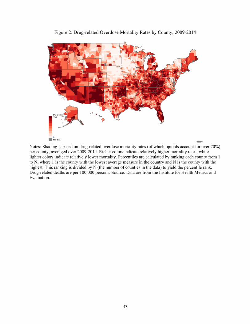
The opioid crisis, as proxied by drug-related mortality rates, has a marked spatial
component. In Figure 2, we display drug-related mortalities by county, averaged over the 2009-
2014 time period, where richer shading indicates relatively higher county-level mortality rates.
Drug-related mortality is notably severe in the Appalachian region, the industrial Midwest,
Oklahoma, Florida, and the Southwest and regions of the Far West. Of the counties which
experienced high to severe increases in the overall number of mortalities between 2000 and
2015, 72 percent were estimated to be rural counties, but only 15 percent of rural counties have a
registered non-profit dedicated to addressing substance abuse (Kneebone & Allard, 2017).2
2 Kneebone and Allard (2017) define a county as having a “high to severe” increase in overdose deaths as one where there were 12 to 28 additional overdose deaths per 100,000 population and caution that data limitations may lead to an undercount of rural non-profits.
6
We display the trend in mean drug-related mortality rates by rurality in Figure 3, panel A.
The mean drug-related mortality rate for rural (red solid line) and nonrural (blue dashed line)
counties are quite similar and track each other closely over the time period. However, the
standard deviations, as shown by dotted lines, increase more for rural areas than for nonrural
areas over time. In Panel B, we see that this differential growth is driven primarily by greater
increases in drug-related deaths at the high end of the distribution of rural counties (see the full
distribution of drug-related deaths for each year in Appendix Figure B1). We calculate the 50th,
75th, 90th, and 99th percentiles in each year for rural (red solid lines) and nonrural (blue dashed
lines) counties and then plot these percentiles over time. The 50th, 75th, and 90th percentile trends
track rather closely across rural and nonrural areas. However, though similar until about 2000,
the 99th percentile in drug-related deaths in rural areas rises more steeply in recent years and is
around 40% higher than in nonrural areas by the end of the period.
Children, Education, and Opioids
Our conceptualization of how the opioid crisis in a community can impact education
outcomes begins with a model proposed by Harding et al. (2010) that relates a neighborhood
factor to a child-level outcome of interest.3 In their model outcome Y is a multiplicative function
of the neighborhood context under consideration, N, exposure level, E, of a child to N, and the
vulnerability of the child, V, given the exposure:
Y = (N x E x V) (1)
3 Our focus in this study is on children who are likely too young to be suffering from substance use disorders themselves. There are children who are exposed to opioids while in utero and may be born experiencing symptoms of opioid withdrawal, a condition known as Neonatal Abstinence Syndrome (NAS). NAS is associated with increased morbidity and incidences of low birthweight, which is itself associated with adverse outcomes, such as developmental delays and language problems, lower education attainment, and lower lifetime earnings (e.g., Behrman and Rosenzweig, 2004; Bharadwaj et al., 2016; Corman and Chaikind, 1998; Patrick et al., 2012; Ribeiro, 2011).

7
Consider Y as some education outcome of interest for a child, N as some measure of the intensity
of the opioid crisis in the child’s community, E as the exposure of the child to crisis, and V as the
vulnerability of the child to the given exposure of the crisis. Variation in exposure across
children can arise from many factors. A child who loses a family member to an opioid overdose
or lives in a home with a family member or members who have an opioid use disorder has higher
levels of exposure than children in the same community who do not have similar experiences.
Less directly, a child who sees ambulances responding to opioid overdoses on their street has
some level of exposure to the crisis, as does finding discarded syringes, hearing parents talk
about opioid-related incidents, or seeing local news about the crisis. And, a child isolated from
these kinds of events may still experience exposure to the crisis if their peer group have crisis
exposure. Thus, childhood exposure to the opioid crisis can range from the direct and traumatic
to the less direct, but still potentially pervasive and destructive.
Moderating the effects of exposure is the vulnerability of a child to the adverse effects of
the crisis, where vulnerability is a function of family, school, and community supports. While
families are considered important to creating safe and nurturing environments that can buffer
children from adverse experiences, communities can also provide critical supports through
formal and informal organizations, structures, and social networks (Shonkoff, 2003). For
example, if suburban or urban communities or schools have a wider array of available support
systems in place than do rural communities, then we might expect a more pronounced effect of
the crisis on education outcomes in rural areas, even with the same levels of crisis intensity and
exposure for a given child.
There is a well-established literature on the effects of childhood exposure to
environmental stressors. While all children are exposed to stress at times, child development

8
experts distinguish between “positive stress” and “tolerable stress” responses, and a “toxic
stress” response in children. Toxic stress responses are consequences of “strong, frequent, or
prolonged activation of the body’s stress response systems” (Shonkoff & Garner, 2012).
Neuroscience research has established that toxic stress can alter the size and neuronal
architecture of the developing brain in young children. These changes can leave a child with
proximate learning and behavioral challenges, and also weaken foundations for later learning,
behavior, and health (Ledoux, 2000; Shonkoff & Garner, 2012).
Childhood environmental conditions are also tightly linked to the formation of a child’s
executive functioning capabilities, defined as mental capacities associated with working
memory, inhibitory control, and cognitive or mental flexibility, and are considered not only
critical for the beginning learner, but healthy development through middle childhood and
adolescence relies on opportunities to build further on these capacities (Center on the Developing
Child at Harvard University, 2011). Research has shown that chaotic and stressful environments
can inhibit executive functioning development and that environments lacking in healthy parent-
child relationships can dampen the development of executive capacities (Barkley, 2001; Evans &
Wachs, 2010; Lengua et al., 2007; Masten & Cicchetti, 2010; Rutter et al., 2000). Therefore,
traumatic or prolonged exposure to stressors can lead to toxic stress response, which in turn can
change the architecture of a child’s developing brain, changes that can have proximate and
lasting effects on physiological, cognitive, behavioral, and/or psychological functioning (e.g.,
Juster et al., 2010; McEwan & Gianaros, 2010).
Research exploring the effects of exposure to neighborhood violence on education
outcomes directly links environmental stressor exposure to adverse education outcomes. Sharkey
et al. (2014) find that students who live on blockfaces where violent crimes occur just before a
9
standardized test perform significantly worse than observationally similar students who live on
blockfaces where violent crimes occur just after an exam. In a similar vein, other work by
Sharkey and colleague’s links exposure to recent local homicides to reductions in children’s
performance on assessments of cognitive skills (Sharkey, 2010; Sharkey et al., 2012).
Meanwhile, Ang (2018) finds that relative to others in their neighborhood, students living
proximate to police officer-involved killings have persistently lower grade point averages, and
immediate, but short-lived, spikes in absenteeism. The path from violence-related trauma to
worse education outcomes is consistent with a toxic stress response explanation.
Despite the now well-published magnitude and extent of the nation’s opioid problem, the
literature on how this public health crisis may be spilling over beyond individuals struggling with
substance use disorder is relatively limited. Quast, Storch, and Yampolskaya (2018) found a
positive association between county-level opioid prescription rates and removal of children from
homes in Florida. Nationally, county-level drug overdose and hospitalization rates are correlated
with both higher child welfare caseloads and high rates of complex child welfare cases (Radel et
al., 2018). Exposure to parental opioid abuse during childhood has been linked to increased risk
for adolescent substance abuse and suicidality (e.g., Biederman et al., 2000; Brent et al., 2019;
Griesler et al., 2019). Meanwhile, Kreuger (2017) links a portion of the fall in labor force
participation among working age men to opioid usage increases. These studies support the
proposition that the ongoing opioid crisis in this country has potentially far reaching and negative
societal effects, particularly on children, that are just beginning to be studied.
The Link Between Opioids and Educational Outcomes
Like the opioid crisis, educational performance is not evenly distributed geographically.
In Figure 4, we display maps that show county-level 3rd grade (Panel A) and 8th grade (Panel B)

10
math and reading standardized test score performance averaged over the 2009-2014 time period
based on data from the Stanford Educational Data Archive (SEDA). Richer shading indicates
relatively lower county-level test scores. As has been well-documented, test scores are generally
lower in the south and southwestern U.S., though there are pockets with higher test scores in
these areas as well as pockets with lower test scores that exist in the rest of the country.
In Figure 5, we display the geographic intersection of 3rd and 8th grade test scores and
drug-related mortality rates. The richer shading in these graphs represent particularly troubling
opioid—education “hot spots:” counties with both relatively high levels of drug-related mortality
rates and relatively low test score performance. The Appalachian Belt again is notable – running
from northern Alabama and Georgia, up into West Virginia, and parts of Ohio, Virginia, and
Pennsylvania. Similarly, the Southwest and West stand out, with troubling hot spots throughout
New Mexico, Arizona, Nevada, and California. Taken together, Figures 2-5 suggest that concern
about how the opioid crisis may be related to children’s education should be more acute in some
areas of the country.
We next consider unconditional correlations between drug-related mortality and
educational outcomes for 3rd grade and 8th grade students. We average mortality rates over
students’ lifetimes to try to capture the overall lifetime intensity of student exposure to the crisis.
Specifically, we average drug mortality rates over the prior 9 years for third grade outcomes (we
call these “mortality rates associated with 3rd graders”) and the prior 14 years for eighth grade
outcomes (“mortality rates associated with 8th graders”). For example, for the year 2009, we
calculate mortality rates associated with 3rd graders as the average of mortality rates from 2000
to 2008 in their county and calculate mortality rates associated with 8th graders as the average of
mortality rates from 1995 to 2008 in their county. As previously discussed, counties with the

11
highest levels of drug-related deaths also had the highest drug-related mortality growth rates,
especially among rural counties. Therefore, the mortality rates associated with 3rd grade students
– averaged over a shorter, more recent set of years – are typically higher than the mortality rates
associated with 8th graders in the same county. The average intensity of average mortality rates
associated with nonrural 3rd graders is higher than those for rural 3rd graders, based on our
measure (see Appendix Table B2); however, the distribution of mortality rates for students living
in rural counties has a longer right tail, reinforcing the need to consider the heterogeneous
experiences students face across counties both within and across rural and nonrural areas.
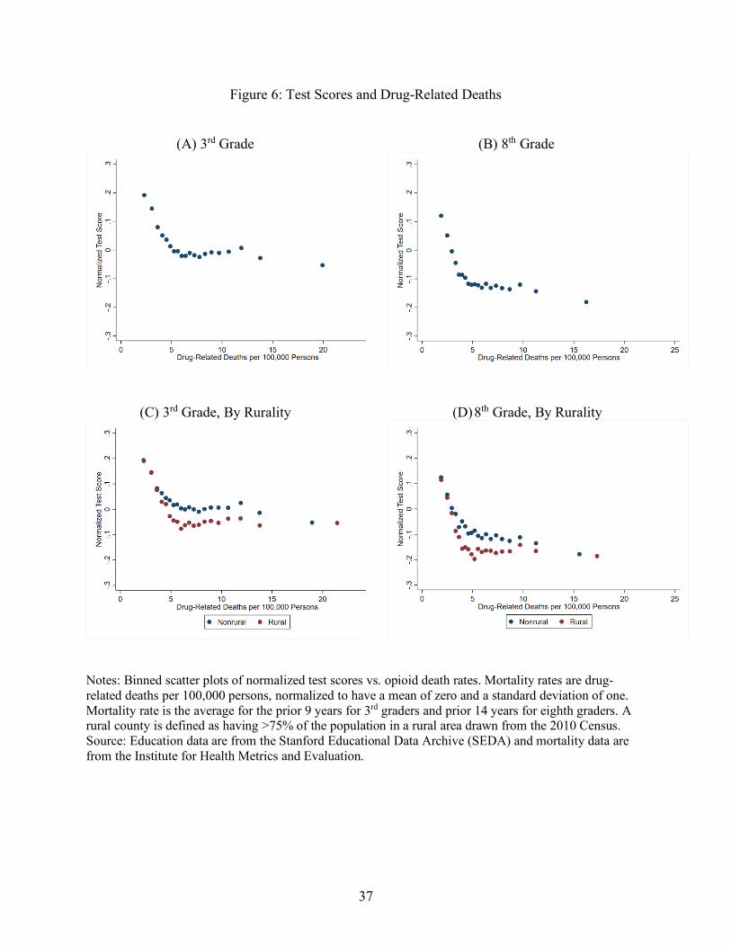
To examine this heterogeneity, consider the bin scatter plots in Figure 6, Panels A and B.
We group mortality rates into twenty equally sized bins (i.e., 5% of counties are in each bin),
with each marker representing the average mortality rate (on the x-axis) and average test score
(on the y-axis) within each bin. For both 3rd and 8th grade, the relationship between test scores
and mortality is negative and non-linear. The test score—mortality gradient is steepest in
counties with mortality rates below the median, which is about 7 deaths per 100,000 persons
over the prior 9 years of 3rd graders in our sample and about 6 deaths per 100,000 persons over
the prior 14 years of 8th graders. After about the median for each sample, the plotted
relationships are slightly downward sloping to flat. In other words, for counties with below-median
mortality rates, the unconditional mortality—test score relationship is steeply negative, but there is less of
a decrease in test scores as you move from lower to higher mortality counties among counties with above-
median mortality rates.
We next consider differences among rural and nonrural areas. There is no universally
accepted definition of rurality. For our main specification, we consider a county to be rural if at
least 75 percent of the county population lives in a rural area (we explore three alternative

12
definitions of rurality in section 7, and Appendix C).4 We display summary statistics for our
sample and by our preferred measure of rurality in Appendix B, Tables 1 and 2. Students in rural
areas are more likely to be white, and counties have fewer college educated residents and lower
household income levels. Rural areas also tend to have a smaller number of schools per county,
lower population density, and lower job density. On average, students in rural counties perform
slightly worse on standardized tests than students in nonrural counties. As previously discussed,
rural counties have slightly lower average mortality rates over the lifetime of students, but
distributions of county-level average lifetime rates for students by rurality illustrate the
complexities of the crisis.
Next, consider the scatter plots by rural and nonrural counties in Figure 6, Panels C and
D. For both rural and nonrural counties, we again see the steepest relationship among counties
with lower levels of opioid intensity, a relationship that flattens out among counties with
relatively high levels of opioid intensity. Rural and nonrural test scores are similar in counties
with the lowest mortality rates, but begin to diverge starting around counties in the 20th
percentile (the fourth bin/dot, moving from left to right on the graph); after this point test scores
in rural counties are always lower than scores in nonrural counties with similar levels of drug-
related mortality.
Estimating the Opioid Crisis—Test Score Relationship
To further understand the relationship between the opioid crisis and education outcomes,
we estimate test scores while controlling for available school district and county characteristics,
4 Based on data from the 2010 Census, where an urban area is defined as an area with a density of at least 1,000 persons square mile and over 2,500 residents, any resident of a county outside of a defined urban area is classified as rural.

13
including per-pupil expenditures, county demographics, poverty rates, and unemployment rates.
Specifically, we estimate:
𝑌𝑌𝑖𝑖𝑖𝑖𝑖𝑖 = 𝛽𝛽0 + 𝛾𝛾𝑀𝑀𝑖𝑖𝑖𝑖 + 𝛽𝛽1𝐸𝐸𝑖𝑖𝑖𝑖 + 𝛽𝛽2𝐶𝐶𝑖𝑖 + 𝛽𝛽2𝑈𝑈𝑖𝑖𝑖𝑖 + 𝑑𝑑𝑖𝑖 + 𝑑𝑑𝑖𝑖 + 𝜀𝜀𝑖𝑖𝑖𝑖𝑖𝑖 (2)
where, Y is educational outcome for county i in state s and year t and M is drug-related mortality
in the county. Our educational outcomes are county average 3rd grade and 8th grade math and
English Language Arts (ELA) test scores in year t. We use mortality rates associated with 3rd
graders and mortality rates associated with 8th graders in our estimates of 3rd and 8th grade test
scores, respectively, to capture the overall lifetime intensity of student exposure to the crisis. As
the majority of drug-related mortality involve opioids, this serves as a proximate measure of the
intensity of the opioid crisis (National Institute on Drug Abuse, 2020). For ease of interpretation
we standardize average mortality rates to have a mean of zero and a standard deviation equal to
one. Results can be interpreted as a one standard deviation change in average mortality rate
associated with 3rd or 8th graders related to a change in test scores. E is a vector of county-level
education measures including:
• Percent in each grade (3rd and 8th) and county of Black/African American students,
Hispanic/Latino students, English language learner students, and Special Education
students;
• Number of schools;
• Number of charter schools;
• Average pupil-teacher ratio; and
• Average expenditures per pupil.
C is a vector of county-level, non-school measures, all from 2010 including:
• Percent with a bachelor’s degree or higher;

14
• Percent foreign born;
• Median household income;
• Percent of households in poverty;
• Percent of single parent households;
• Percent non-white race/ethnicity;
• Population density;
• Total population;
• Total area (in millions of square miles); and
• Percent rural population.
U is a vector of county-level economic measures including:
• Unemployment rate;
• Annualized job growth 2004-2013; and
• Job density in 2013.
We also include year, 𝑑𝑑𝑖𝑖, and state, 𝑑𝑑𝑖𝑖, fixed effects and cluster standard errors by state. We
clustered at the higher level of clustering (state instead of county) because many policies related
to opioids are enacted at a state level, and because we view this as the more conservative
approach. However, inferences are similar when clustering at a county level, and in most cases
lead to more precise estimates.
We do not include county fixed effects in the regression because they would remove the
most amount of variation in our educational outcomes and measures of mortality over our time
period, and more importantly, the variation on which we are primarily focused in this paper,
which is across-county variation. About 83 and 85 percent of the 3rd and 8th grade test score
variation in our data is cross-sectional, respectively, while about 16 and 14 percent is within

15
county variation over time (the remaining variation is the contribution of the national time trend).
About 94 and 92 percent of the variation in mortality rates associated with 3rd graders and 8th
graders, respectively, is cross-sectional, as compared to just 2 percent that is due to within county
variation over time. Recall that we average mortality rates over students’ lifetimes in an attempt
to capture the overall lifetime intensity of student exposure to the crisis, which is part of the
reason there is little over-time variation in the mortality rates that we use.
We interpret estimates of 𝛾𝛾 from this model as the extent to which test scores and
mortality rates covary conditional on included covariates, not as causal estimates of the effect of
the opioid crisis on test scores. There are numerous unobserved factors that could be correlated
with both academic outcomes and drug-related mortality. Our intention in this paper is to better
understand the relationship between the opioid crisis and education, and to explore the extent to
which that relationship may be different for rural and nonrural counties. Planned future work
exploits naturally occurring events to better identify causal relationships between the crisis and
education outcomes.
To explore the extent to which there may be correlational differences by rurality, we add
to equation (2) a rural indicator, where we define rural counties (R = 1) as counties where at least
75 percent of the population live in a rural area. We use estimates based on equation (3) to
explore the rural nature of the opioid crisis:
Yits = β0 + 𝛾𝛾1𝑀𝑀𝑖𝑖𝑖𝑖 + 𝛾𝛾2(𝑀𝑀 × 𝑅𝑅)𝑖𝑖𝑖𝑖 + β1Eit + β2Ci + β2Uit + β3Ri + dt + ds + εits (3)
From these estimates, we interpret 𝛾𝛾2 as the as the increment (decrement) to the conditional
relationship between test scores and mortality rates in rural counties relative to this relationship
in nonrural counties as captured by 𝛾𝛾1. We can recover the “total” conditional relationship
between test scores and mortality rates in rural counties as the linear combination of 𝛾𝛾2 and 𝛾𝛾1.

16
Finally, to understand whether conditional relationships are nonlinear (as the
unconditional graphs in Figure 6 suggest), we also substitute a vector of indicators for deciles of
mortality rates for M in equations (2) and (3). We set the coefficient for the first decile (i.e., the
counties with mortality rates in the lowest ten percent) to be equal to zero, such that coefficients
on each of the indicators for the second to tenth deciles are estimates of how much lower the test
scores are in counties with drug-related mortality rates in that decile, relative to the first decile.
Findings
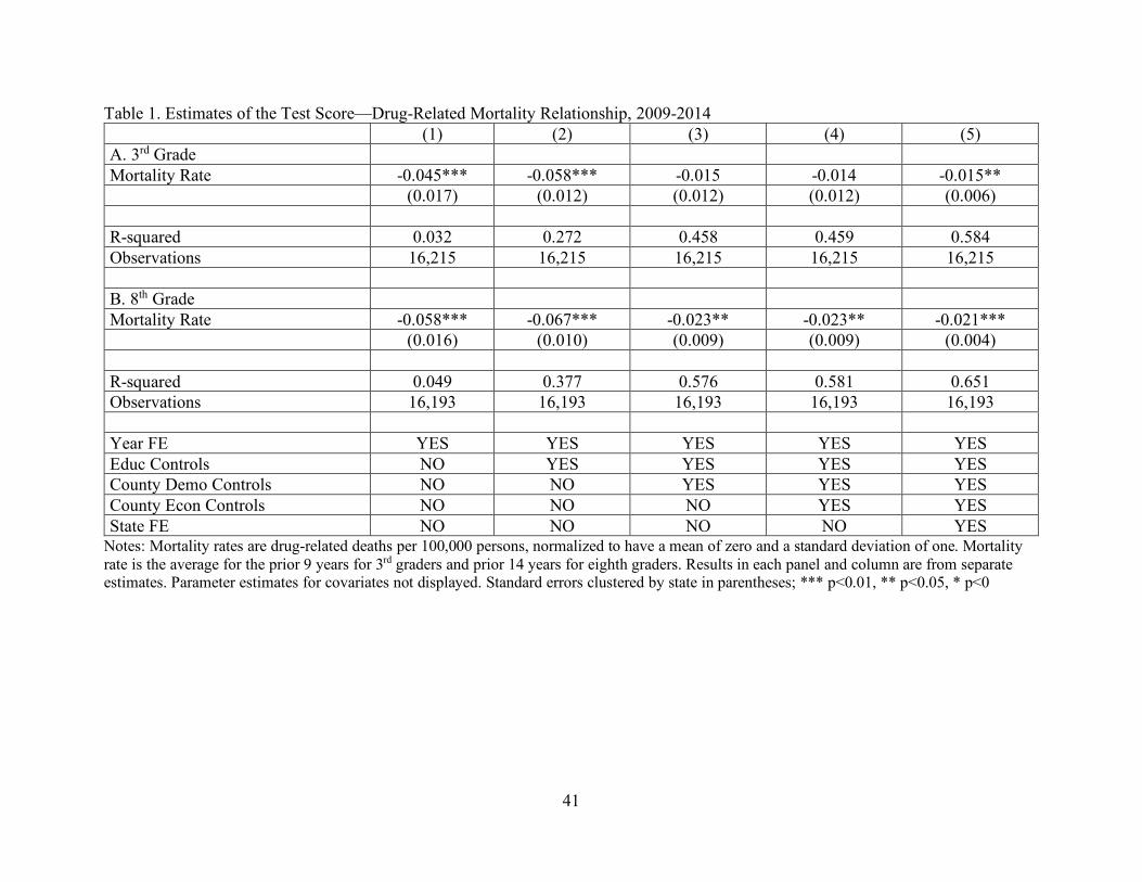
We display estimates of equation (2) in Table 1 where columns 1 through 5 represent
estimates from models that have increasing sets of control variables. First consider the estimates
for 3rd grade test scores displayed in Panel A of Table 1. Counties with higher mortality rates by
one standard deviation have 0.045 standard deviations lower 3rd grade test scores. As we add
education characteristics in column 2, point estimates increase to -0.058 (though this coefficient
is not statistically different than the one in column 1); coefficients attenuate to -0.015 once we
add county demographic characteristics in column 3 and are no longer statistically significant.
Point estimates remain similar with the addition of county economic characteristics in column 4
and state fixed effects in column 5, with the result statistically significant in our preferred model
in column 5. The inclusion of state fixed effects account for a portion of the residual variation,
resulting in more precise point estimates.
We display corollary results for 8th grade test scores in Panel B. Estimates with only year
fixed effects yield a result in column 1 that counties with higher mortality rates by one standard
deviation have lower 8th grade test scores of 0.058 standard deviations. Similar to 3rd grade, the
coefficient gets larger when we add education controls, to 0.067, though again this is not
statistically different than the result in column 1. Results then attenuate to about -0.021 to -0.023

17
in columns 3 through 5, all statistically significantly different than zero, with our preferred model
indicating that counties with counties with higher mortality rates by one standard deviation have
lower 8th test scores of 0.21 standard deviations. In results not displayed for brevity but available
upon request, we find generally similar results when examining ELA and math test scores
separately, though the point estimates for math scores are slightly larger in magnitude than for
ELA.
We next display results from our analysis of potentially differential relationships between
rural and nonrural areas in Table 2. Our results, using just our preferred specification, are
suggestive evidence that the test score-opioid gradient is steeper in rural than in nonrural
counties for younger students. Our estimate of the test score—overdose link relationship among
3rd graders is -0.016 (in column 1), with the corresponding 8th grade estimate smaller (-0.004)
and not statistically significant. This again suggests potentially different mechanisms at play at
different grade levels.
In Figure 7, we present results that allow for the mortality-test score relationship to differ
between rural and nonrural counties nonparametrically. We see that among both rural and
nonrural counties, and as we first saw in Tables 1 and 2, test scores and mortality rates are
negatively related. The estimated test scores for rural counties are always lower than those of
nonrural counties (though not statistically different in most cases). Both panels indicate the rural-
nonrural gap appears to grow as mortality levels increase, with an especially pronounced, though
less precise, growing gap among third graders. The estimated gaps between rural and nonrural
students are only statistically different among 3rd grade students living in counties with the
highest drug-related mortality rates (8th, 9th, and 10th deciles). These results offer suggestive
evidence that the role of the opioid crisis in affecting educational outcomes may be especially
18
concerning in rural areas and, particularly, in rural areas with especially high drug-related
mortality rates. The magnitude of that difference is noteworthy: rural counties in the highest
(10th) deciles of drug-related mortality have 3rd grade test scores that are almost two tenths of a
standard deviation lower than rural counties in the lowest (1st) decile. The contrast appears
especially stark when compared to the analogous difference for nonrural counties which is half
as large.
We display the average drug-related mortalities per 100,000 persons within each decile
associated with each grade in Appendix Table B3. In that table there is a notable jump from the
9th to 10th decile in the 9-year average drug-related mortality measure we associate with 3rd grade
test scores (reflecting the recent rise in hard hit counties in more recent years as we show in
Figure 3). This might explain why we observe a relatively large coefficient for the 10th decile in
panel A – the students who live in these hardest hit rural counties face a disproportionately large
opioid epidemic that could be impeding educational achievement.
Students within a community could be affected differentially by the opioid crisis. To
investigate this, we next consider how opioids relate to achievement gaps between students who
are and are not considered economically disadvantaged (ECD). We use the measure of economic
disadvantage available in the Stanford Educational Data Archive, which is based on states’ own
definitions. If economically disadvantaged students have fewer familial resources to insure their
children against exposure to the opioid crisis, as suggested in our conceptual framework, we may
see NonECD—ECD gaps widen as exposure to the crisis increases, a relationship we examine in
Table 3. The point estimates are consistently small and statistically insignificant, suggesting that
on average, higher opioid mortality rates are not differentially related to students test scores
based on broad categorizations of economic status.
19
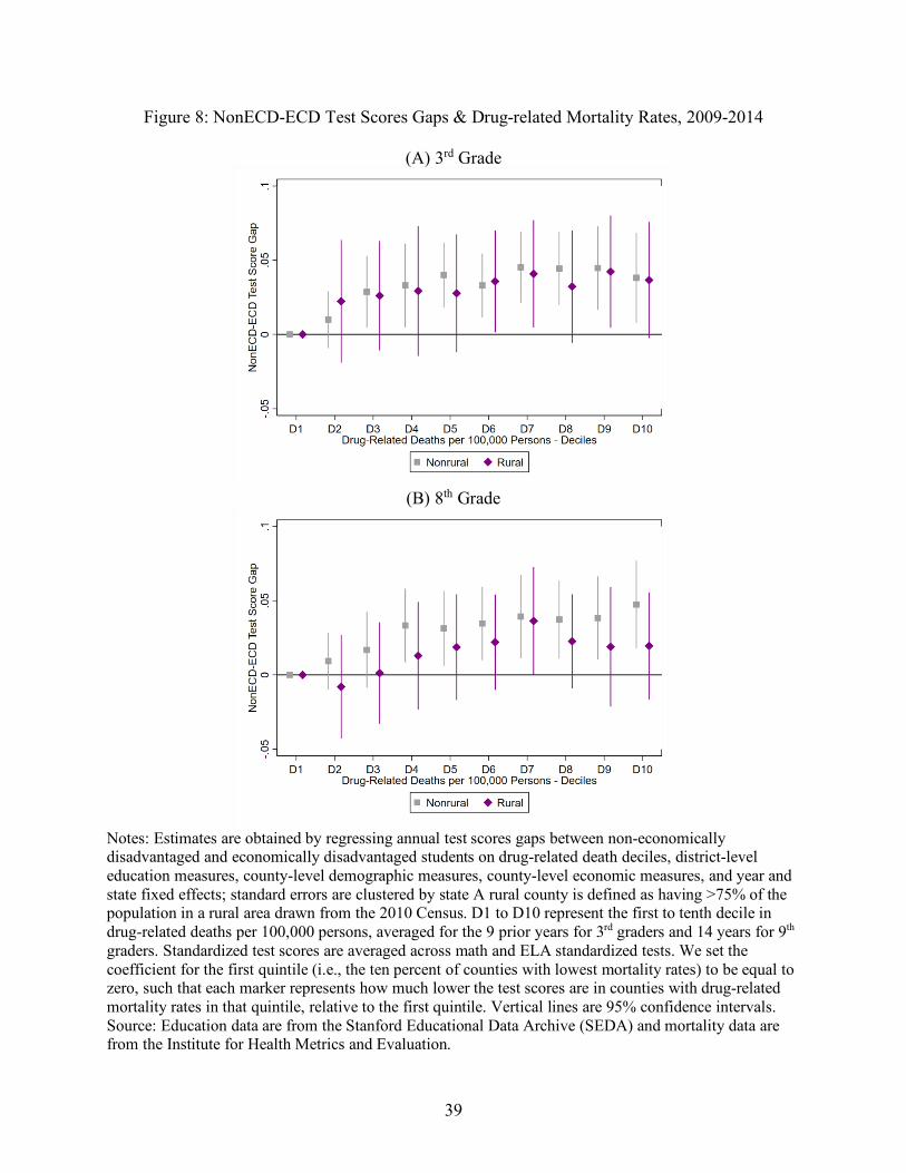
In Figure 8, we further consider this question by examining ECD status by decile of
mortality rates. Similar to Figure 7, we set the coefficient for the first decile to be equal to zero,
such that each marker represents, at that decile in mortality rate, the gap in scores between less
and more economically disadvantaged students relative to that gap in the first decile of mortality.
As seen in both panels, the NonECD—ECD gap is generally lowest in the first decile, though the
point estimates are only mildly increasing from left to right and confidence intervals generally
overlap zero for rural students. The coefficients for nonrural 3rd and 8th grade students are
statistically different from zero starting with the 3rd decile and 4th decile, respectively, with the
magnitude of the point estimates remaining similar across mortality rate deciles.
Taken together, among nonrural students, there is mild evidence of a NonECD—ECD
gap in areas with higher levels of the opioid crisis; however, results do not reveal a strong pattern
to suggest that rural ECD students have lower test scores on average when exposed to similar
levels of the opioid crisis as compared to their NonECD peers within the same county. We
proffer a few possible explanations for these findings. It could be that the measures of economic
disadvantage we use do not correspond well to vulnerability to the opioid epidemic. The SEDA
ECD measure is highly correlated with free and reduced-price lunch (FRPL) status (Fahle et al.,
2018). Though commonly used, there is some question about how well point-in-time FRPL
status measures disadvantage more broadly (e.g., Domina et al., 2018; Michelmore & Dynarski,
2017; Koedel & Parsons, 2020), and more work is needed to identify the factors that leave
children vulnerable specifically to the opioid crisis. Another issue could be variation in
disadvantage identification across states that introduces error in a national analysis. For example,
in Florida, FRPL students are considered ECD, while in Massachusetts students are defined as
ECD if they participate in a program such as the foster care system or SNAP ((Florida
20
Department of Education, n.d.; Massachusetts Department of Elementary and Secondary
Education, n.d.). Beyond measurement, it is also possible that community- and school-level
conditions, supports, and programs mitigate the effects of family supports or resource
constraints. This is clearly a question that deserves examination in future work.
Alternative Definitions of Rurality
In our preferred definition, we classify a county as rural if over 75% of the population
lives in a rural area. We employ three additional measures of rurality based on commonly
employed rural classification schemes. Waldorf and Kim (2015) suggest that rurality is
characterized by population size and density, with lower population and lower density indicative
of greater rurality. Additionally, remoteness, or distance from concentrated population centers, is
often conceptualized as a dimension of rurality. In our case we wish to see whether the
characteristics of rurality and rural education such relative isolation and lower social service
provision interact with the opioid overdose crisis and are associated with differential outcomes
compared to less rural areas.
In the first alternative definition, we define rural as counties which are classified as
noncore counties under Office of Management and Budget (OMB) guidelines; these are counties
which are not contained within a metropolitan or micropolitan statistical area.5 This noncore
definition is employed by the National Center for Health Statistics to identify the most rural
areas in the country (CDC, 2017). In our second alternative definition, we use a measure of deep
rurality drawn from the Economic Research Service (ERS) rural-urban continuum classification.
The ERS classification expands upon OMB county designations with a greater number of
5 Metropolitan areas are central counties and outlying counties with strong commuting ties and an urban population of over 50,000 while micropolitan areas follow the same definition but for counties with greater than 10,000 residents in an urban area.
21
categories based on population and remoteness. We define deep rurality as counties which are
classified as the most rural according to the ERS; these are counties which are completely rural
or have less than 2,500 residents in urban areas (United States Department of Agriculture, 2019).
Finally, in the third alternative definition, we employ National Center for Education Statistics
(NCES) school classifications to capture the share of students who attend a school classified as
rural in each county. We mirror our main specification and define a county as rural if more than
75% of students in a county attend a school which is classified as rural.
Our three alternative definitions of rurality capture a general continuum of relative
rurality (see Appendix Tables C1-C3 and Appendix Figure C1). The noncore definition is the
broadest definition of rural, with about 79% of the population in counties, based on percentage of
residents in a county that live in a rural area drawn from 2010 Census, defined as rural living in
rural areas. On the other end of the spectrum, about 99% of the population living in counties
identified under our deep rurality definition live in rural areas. The third definition, based on
NCES, lies between these two measures, with about 90% of the population living in counties
identified as rural under alternative definition 3.
In Table 4 we display the estimated test scores—drug-related mortality rate relationships
for the alternative rurality definitions. Estimates of the relationship between mortality and test
scores for nonrural counties remain directionally consistent across specifications and with our
preferred measure. The negative relationship between test scores and overdose mortality for 3rd
grade students in rural counties increases as the share of rural residents per the 2010 Census
increases. This association ranges from a statistically insignificant -0.007 with the noncore
definition and -0.010 using the NCES classification to a statistically significant -0.032 for 3rd
grade students in deeply rural counties. These results taken in combination with our main

22
specification suggest that the extent of negative relationship between rural students and poorer
outcomes grows as counties become increasingly rural as defined by Census share of rural
residents. All of the rural coefficients for 8th grade students are negative but statistically
insignificant, though they trend in the same direction as the estimates for 3rd grade students with
consistently lower point estimates as rurality increases.
Discussion
To our knowledge this is the first use of national data to examine the relationship
between the nation’s opioid crisis and the education outcomes of our children. To this point,
much of the opioid epidemic research has been focused on those most directly impacted by the
epidemic: individuals with opioid substance use disorder. Our research agenda focus has been
less proximate as we ask: what happens to the education of children who live in communities
where the opioid crisis has taken hold? In this case we have focused on the collateral damage
that impacts children and potentially manifests in measurably reduced learning outcomes. Our
evidence suggests a need to be aware of the potentially negative effects of the crisis on the
education outcomes of children, particularly in the hardest hit areas, many of which are
considered rural.
While these estimates offer suggestive evidence that exposure to the opioid crisis and its
collateral consequences negatively impacts the learning of children, we caution that they do not
establish the causal conclusions that are better suited to inform policy initiatives. For brevity, in
this paper we have examined only 3rd and 8th grade test scores; however, it is likely that
detrimental educational effects of exposure to the opioid crisis vary depending on the age and
developmental stage of the child or young adult. Exposure to the epidemic is likely to impact
important education outcomes other than test scores such as attendance, probability of school
23
disciplinary action, graduation, or college enrollment. Future investigations into a broader set of
outcomes would be a fruitful inquiry.
In addition to potential age-related differences in the impact of the epidemic on children’s
learning, the issue of cumulative exposure versus immediate exposure is an avenue that also
warrants further study. That is, to what extent does it matter that, say, a 3rd grader has grown up
in a community that has persistently dealt with the epidemic for many years relative to a 3rd
grader who finds her or his self in a community that has been more recently engulfed in the
opioid epidemic. Given variation in the timing of the introduction of large amounts of opioids
into communities as a result of pharma distribution decisions or local pharmacy and physician
dispensation practices, we are exploring the respective roles of cumulative versus more recent
exposure in ongoing work.
With those caveats in mind, graphically and with conditional estimates we have shown
strong correlations between counties that have high drug-related mortality rates and counties
with worse education outcomes among both 3rd and 8th grade students. At least for 3rd grade
students, these relationships appear to increase as the depth of the opioid crisis in a county
increases and in areas with higher degrees of rurality. The concept of what it means to be rural is
nuanced given the different ways in which rurality can be defined. In recognition of this fact, we
examine multiple potential definitions of rurality. 3rd grade students in the most rural parts of the
country appear to have the worst educational outcomes in the face of the opioid crisis when
compared with both their nonrural peers and corresponding 8th grade cohorts. In order to further
examine the rural education-opioid crisis link, future work would be well served to examine
rurality at a finer level, as aggregate county level measures of rurality may miss out on variation
which is key to understanding the relationship in question.

24
It is beyond the scope of this paper to recommend specific support mechanisms through
which states, school districts, and schools could respond to the problem at hand, and we are
cautious to avoid strong recommendations since there is limited evidence on the efficacy of
current attempted solutions. We view this paper instead as a first step in raising awareness of the
potential collateral damage of the opioid epidemic. Nonetheless, our opioid-education model can
offer some suggestions regarding possible points of intervention.
Our previously described conceptual framework allows the opioid epidemic to negatively
affect children through the interaction of their exposure and their vulnerability given exposure. It
would be difficult for schools to address a child’s direct exposure to the epidemic because of
what may be happening in the child’s home or community. However, schools potentially have a
role to play in reducing the vulnerability of their students to the aftermath of these experiences or
incidents. For example, children may be better positioned to deal with trauma if they have
greater access to school counselors and support personnel. The emergence of the “trauma-
sensitive school” model is one promising approach to providing school-based supports aimed at
helping students cope with trauma (Jones et al., 2018). Schools could also reduce vulnerability
by coordinating with other community services. For example, the Handle with Care program in
Charleston, West Virginia and replicated elsewhere works to coordinate emergency responders
and local school officials so that if, for example, emergency personnel respond, for any reason,
to an address where a minor child is present, school officials will be notified before the start of
the next school day. Thus, school personnel will be more aware that a child had or witnessed a
potentially traumatic experience and will be “handled with care” as per the training of school
personnel that is a part of the program.

25
A challenge associated with building such supports to reduce children’s vulnerability to
the opioid crisis is that school and community resources are not distributed equally across
geographic regions. The opioid crisis is particularly acute in areas that are also experiencing
other types of hardship, such as challenging economic and job market conditions. These
conditions can tax available community and health supports and can also affect resources
available to schools. We display two measures of school resources from the 2013-2014 school
year in Figure 9: local revenue (panel A) and total expenditures (panel B) per student. Local
revenue is largely a function of local property taxes, which can be supplemented by state and
federal sources to fund total expenditures. Examining school district revenue reveals a troubling
pattern: many of the communities where children have the highest exposure to the opioid crisis
also have relatively low revenue levels, potentially limiting the assistance and programs schools
can offer to reduce children’s vulnerability.
This paper presents a new and potentially troubling side of the nation’s opioid crisis,
namely, the adverse effects this scourge may be having on the learning potential of our children.
We view this as a first step in examining the connections between the opioid crisis and education
outcomes, and these findings suggest a need for further research on several fronts. A next research
step is to better establish causal connections between the crisis and education outcomes. To do this
requires variation in the intensity of the opioid epidemic across time or place that is “exogenous”
or plausibly unrelated to other factors that drive education outcomes. While there are challenges
to identifying such variation, there are some potential avenues for researchers. For example, we
are currently working with data from Florida where we examine how plausibly exogenous
variation in opioid-related measures like mortalities, emergency room visits, and pill distributions,
brought about by legislatively induced “pill mill” closures, affects the education outcomes of

26
children. Research into the mechanisms through which the crisis impacts the learning in of children
should follow. Finally, programs and policies through which children’s vulnerabilities to the
effects of the crisis can be mitigated, along with the role of resource constraints in establishing
effective programs and policies are areas worthy of research.
References
Ang, D. (2018). The effects of police violence on inner-city students. (Working Paper). https://pdfs.semanticscholar.org/a6ea/d685255658b4e931a6ff3448d03b0a806387.pdf
Barkley, R. A. (2001). The executive functions and self-regulation: An evolutionary neuropsychological perspective. Neuropsychology Review, 11(1), 1-29. https://doi.org/10.1023/A:1009085417776
Behrman, J. R., & Rosenzweig, M. R. (2004). Returns to birthweight. Review of Economics and Statistics, 86(2), 586-601. https://doi.org/10.1162/003465304323031139
Bharadwaj, P., Lundborg, P., & Rooth, D. O. (2018). Birth weight in the long run. Journal of Human Resources, 53(1), 189-231. https://doi.org/10.3368/jhr.53.1.0715-7235r
Biederman, J., Faraone, S. V., Monuteaux, M. C., & Feighner, J. A. (2000). Patterns of alcohol and drug use in adolescents can be predicted by parental substance use disorders. Pediatrics, 106(4), 792-797. https://doi.org/10.1542/peds.106.4.792
Brent, D. A., Hur, K., & Gibbons, R. D. (2019). Association between parental medical claims for opioid prescriptions and risk of suicide attempt by their children. JAMA Psychiatry, 76(9), 941-947. https://doi.org/10.1001/jamapsychiatry.2019.0940
Case, A., & Deaton, A. (2017). Mortality and morbidity in the 21st century. Brookings Papers on Economic Activity, 2017(1), 397-476. https://doi.org/10.1353/eca.2017.0005
Center on the Developing Child at Harvard University (2011). InBrief: The Impact of Early Adversity on Children's Development. The InBrief Series. https://developingchild.harvard.edu/resources/inbrief-the-impact-of-early-adversity-on-childrens-development-video/
Centers for Disease Control and Prevention, National Center for Injury Prevention and Control. (2018a, December 19). Understanding the Epidemic. https://www.cdc.gov/drugoverdose/epidemic/index.html
Centers for Disease Control and Prevention, National Center for Injury Prevention and Control. (2018b, October 3). U.S. Opioid Prescribing Rate Maps. https://www.cdc.gov/drugoverdose/maps/rxrate-maps.html
Centers for Disease Control and Prevention, National Center for Injury Prevention and Control. (2019, June 27). Drug Overdose Deaths. https://www.cdc.gov/drugoverdose/data/statedeaths.html
Centers for Disease Control and Prevention, National Center for Health Statistics. (2017, June 1). NCHS Urban-Rural Classification Scheme for Counties. https://www.cdc.gov/nchs/data_access/urban_rural.htm
28
Corman, H., & Chaikind, S. (1998). The effect of low birthweight on the school performance and behavior of school-aged children. Economics of Education Review, 17(3), 307-316. https://doi.org/10.1016/s0272-7757(98)00015-6
Dasgupta, N., Beletsky, L., & Ciccarone, D. (2018). Opioid crisis: no easy fix to its social and economic determinants. American Journal of Public Health, 108(2), 182-186. https://doi.org/10.2105/ajph.2017.304187
Department of Health and Human Services. (2019, September 4). What is the U.S. Opioid Epidemic? https://www.hhs.gov/opioids/about-the-epidemic/index.html
Dwyer-Lindgren, L., Bertozzi-Villa, A., Stubbs, R. W., Morozoff, C., Shirude, S., Unützer, J., ... & Murray, C. J. (2018). Trends and patterns of geographic variation in mortality from substance use disorders and intentional injuries among US counties, 1980-2014. Jama, 319(10), 1013-1023.
Evans, G., & Wachs, T. (2010). Chaos and its influence on children's development: An ecological perspective (1st ed.). Washington, DC: American Psychological Association. https://doi.org/10.1037/12057-000
Fahle, E.M., Shear, B.R., Kalogrides, D., Reardon, S.F., Chavez, B., & Ho, A.D. (2018). Stanford Education Data Archive: Technical Documentation (Version 3.0). http://purl.stanford.edu/db586ns4974
Florida Department of Education. (n.d.). Definitions. https://edstats.fldoe.org/portal%20pages/Documents/Definitions.pdf
García, M.C., Heilig, C.M., Lee, S.H., Faul, M., Guy, G., Iademarco, M.F., Hempstead, K., Raymond, D., Gray, J. (2019). Opioid prescribing rates in nonmetropolitan and metropolitan counties among primary care providers using an electronic health record System — United States, 2014–2017. Washington DC: Centers for Disease Control and Prevention. http://dx.doi.org/10.15585/mmwr.mm6802a1external icon.
Goodwin, J. S., Kuo, Y. F., Brown, D., Juurlink, D., & Raji, M. (2018). Association of chronic opioid use with presidential voting patterns in US counties in 2016. JAMA Network Open, 1(2), e180450-e180450. https://doi.org/10.1001/jamanetworkopen.2018.0450
Griesler, P. C., Hu, M.-C., Wall, M. M., & Kandel, D. B. (2019). Nonmedical prescription opioid use by parents and adolescents in the US. Pediatrics, 143(3), 1-10. https://doi.org/10.1542/peds.2018-2354
Hancock, C., Mennenga, H., King, N., Andrilla, H., Larson, E., & Schou, P. (2017). Treating the rural opioid epidemic. National Rural Health Association. https://www.ruralhealthweb.org/NRHA/media/Emerge_NRHA/Advocacy/Policy%20documents/2019-NRHA-Policy-Document-Treating-the-Rural-Opioid-Epidemic.pdf
Harding, D. J., Gennetian, L., Winship, C., Sanbonmatsu, L., & Kling, J. R. (2010). Unpacking neighborhood influences on education outcomes: Setting the stage for future
29
research (No. w16055). National Bureau of Economic Research. https://doi.org/10.3386/w16055
Health Resources and Services Administration. (2018, December). Defining Rural Population. https://www.hrsa.gov/rural-health/about-us/definition/index.html
Ingram, D. D., & Franco, S. J. (2014). 2013 NCHS urban-rural classification scheme for counties (No. 2014). US Department of Health and Human Services, Centers for Disease Control and Prevention, National Center for Health Statistics.
Jones, W.J., Berg, J., & Osher, D. (2018). Trauma and Learning Policy Initiative (TLPI): Trauma-Sensitive Schools Descriptive Study. Washington, DC: American Institutes for Research. https://traumasensitiveschools.org/wp-content/uploads/2019/02/TLPI-Final-Report_Full-Report-002-2-1.pdf
Juster, R.-P., McEwen, B. S., & Lupien, S. J. (2010). Allostatic load biomarkers of chronic stress and impact on health and cognition. Neuroscience & Biobehavioral Reviews, 35(1), 2-16. https://doi.org/10.1016/j.neubiorev.2009.10.002
Kneebone, E., & Allard, S. W. (2017, September 25). A nation in overdose peril: pinpointing the most impacted communities and the local gaps in care. Washington, DC: The Brookings Institute. https://www.brookings.edu/research/pinpointing-opioid-in-most-impacted-communities/
Koedel, C., & Parsons, E. (2020). The Effect of the Community Eligibility Provision on the Ability of Free and Reduced-Price Meal Data to Identify Disadvantaged Students (Vol. 320). CALDER Working Paper No. 234.
Kohomban, J., Rodriguez, J., & Haskins, R. (2018, January 31). The foster care system was unprepared for the last drug epidemic—let’s not repeat history. Washington, DC: The Brookings Institute. https://www.brookings.edu/blog/up-front/2018/01/31/the-foster-care-system-was-unprepared-for-the-last-drug-epidemic-lets-not-repeat-history/
Krueger, A. B. (2017). Where have all the workers gone? An inquiry into the decline of the US labor force participation rate. Brookings Papers on Economic Activity, 2017(2), 1. https://doi.org/10.1353/eca.2017.0012
LeDoux, J. E. (2000). Emotion circuits in the brain. Annual Review of Neuroscience, 23(1), 155-184. https://doi.org/10.1146/annurev.neuro.23.1.155
Lengua, L. J., Honorado, E., & Bush, N. R. (2007). Contextual risk and parenting as predictors of effortful control and social competence in preschool children. Journal of Applied Developmental Psychology, 28(1), 40-55. https://doi.org/10.1016/j.appdev.2006.10.001
Massachusetts Department of Elementary and Secondary Education. (n.d.) Redefining Low Income – A New Metric for K-12 Education. http://www.doe.mass.edu/infoservices/data/ed.html

30
Masten, A. S., & Cicchetti, D. (2010). Developmental cascades. Development and Psychopathology, 22(3), 491-495. https://doi.org/10.1017/s0954579410000222
Michelmore, K., & Dynarski, S. (2017). The gap within the gap: Using longitudinal data to understand income differences in educational outcomes. AERA Open, 3(1), 1-18.McEwen, B., & Gianaros, P. (2010). Central role of the brain in stress and adaptation: Links to socioeconomic status, health, and disease. Annals of the New York Academy of Sciences, 1186, 190-222. https://doi.org/10.1111/j.1749-6632.2009.05331.x
National Institute on Drug Abuse. (2020, March). Overdose Death Rates. https://www.drugabuse.gov/related-topics/trends-statistics/overdose-death-rates
Patrick, S. W., Schumacher, R. E., Benneyworth, B. D., Krans, E. E., McAllister, J. M., & Davis, M. M. (2012). Neonatal abstinence syndrome and associated health care expenditures: United States, 2000-2009. JAMA, 307(18), 1934-1940. https://doi.org/10.1001/jama.2012.3951
Quast, T., Storch, E. A., & Yampolskaya, S. (2018). Opioid prescription rates and child removals: evidence from Florida. Health Affairs, 37(1), 134-139. https://doi.org/10.1377/hlthaff.2017.1023
Radel, L., Baldwin, M., Crouse, G., Ghertner, R., & Waters, A. (2018). Substance use, the opioid epidemic, and the child welfare system: Key findings from a mixed methods study. Washington, DC: Office of the Assistant Secretary for Planning and Evaluation. https://bettercarenetwork.org/sites/default/files/SubstanceUseChildWelfareOverview.pdf
Ribeiro, L. A., Zachrisson, H. D., Schjolberg, S., Aase, H., Rohrer-Baumgartner, N., & Magnus, P. (2011). Attention problems and language development in preterm low-birth-weight children: Cross-lagged relations from 18 to 36 months. BMC pediatrics, 11(1), 59. https://doi.org/10.1186/1471-2431-11-59
Rummans, T. A., Burton, M. C., & Dawson, N. L. (2018, March). How good intentions contributed to bad outcomes: the opioid crisis. In Mayo Clinic Proceedings (Vol. 93, No. 3, pp. 344-350). Elsevier. https://doi.org/10.1016/j.mayocp.2017.12.020
Rutter, M. L., Kreppner, J. M., & O'Connor, T. G. (2001). Specificity and heterogeneity in children's responses to profound institutional privation. The British Journal of Psychiatry, 179(2), 97-103. https://doi.org/10.1192/bjp.179.2.97
Sharkey, P., Schwartz, A. E., Ellen, I. G., & Lacoe, J. (2014). High stakes in the classroom, high stakes on the street: The effects of community violence on students’ standardized test performance. Sociological Science, 1, 199-220. https://doi.org/10.15195/v1.a14
Sharkey, P. (2010). The acute effect of local homicides on children's cognitive performance. Proceedings of the National Academy of Sciences, 107(26), 11733-11738. https://doi.org/10.1073/pnas.1000690107
31
Sharkey, P., Tirado-Strayer, N., Papachristos, A., & Raver, C. C. (2012). The effect of local violence on children’s attention and impulse control. American Journal of Public Health, 102(12), 2287-2293. https://doi.org/10.2105/ajph.2012.300789
Shonkoff, J. P. (2003). From neurons to neighborhoods: old and new challenges for developmental and behavioral pediatrics. Journal of Developmental & Behavioral Pediatrics, 24(1), 70-76. https://doi.org/10.1097/00004703-200302000-00014
Shonkoff, J., & Garner, A. (2012). The lifelong effects of early childhood adversity and toxic stress. Pediatrics, 129(1), e232-246. https://doi.org/10.1542/peds.2011-2663
United States Department of Agriculture, Economic Research Service. (2019, October 25). Rural-Urban Continuum Codes: Documentation. https://www.ers.usda.gov/data-products/rural-urban-continuum-codes/documentation/
Waldorf, B., & Kim, A. (2015). Defining and measuring rurality in the US: From typologies to continuous indices. In Commissioned Paper Presented at the Workshop on Rationalizing Rural Area Classifications, Washington, DC. https://sites.nationalacademies.org/cs/groups/dbassesite/documents/webpage/dbasse_167036.pdf
Wolke, D., Eryigit-Madzwamuse, S., & Gutbrod, T. (2014). Very preterm/very low birthweight infants’ attachment: infant and maternal characteristics. Archives of Disease in Childhood-Fetal and Neonatal Edition, 99(1), F70-F75. https://doi.org/10.1136/archdischild-2013-303788

32
Figure 1: County Level Drug-Related Mortality Rate Trends
(A) Mean Drug-Related Mortality Rates per 100,000 Persons
(B) Trends in Drug-Related Deaths per 100,000 Persons, Quartiles of 2014 Mortality Rate
Notes: Panel (A): Solid lines are the county mean per year; dashed lines are standard deviations around the mean. Panel (B): Counties are divided into quartiles based on 2014 mortality rates. Drug-related deaths are per 100,000 persons. Source: Data are from the Institute for Health Metrics and Evaluation.
33
Figure 2: Drug-related Overdose Mortality Rates by County, 2009-2014
Notes: Shading is based on drug-related overdose mortality rates (of which opioids account for over 70%) per county, averaged over 2009-2014. Richer colors indicate relatively higher mortality rates, while lighter colors indicate relatively lower mortality. Percentiles are calculated by ranking each county from 1 to N, where 1 is the county with the lowest average measure in the country and N is the county with the highest. This ranking is divided by N (the number of counties in the data) to yield the percentile rank. Drug-related deaths are per 100,000 persons. Source: Data are from the Institute for Health Metrics and Evaluation.

34
Figure 3: Drug-Related Mortality Rate Trends by Rurality, 1995—2014
(A) Mean Drug-Related Mortality Rates, by Rurality
(B) Trends in Drug-Related Deaths, by Rurality Selected Percentiles
Notes: Panel (A): Mean drug-related deaths per 100,000 persons displayed by rurality. Rural death rate indicated by solid red line, nonrural death rate indicated by dashed blue line. Standard deviations are dotted lines in corresponding colors. Panel (B): Median (circle), 75th (diamond), 90th (square), and 99th (triangle) percentiles of drug-related deaths per 100,000 by rurality. Percentiles are calculated separately for each year. Nonrural measures are in blue while rural measures are in red. For both panels, a rural county is defined as having >75% of the population in a rural area drawn from the 2010 Census. Source: Data are from the Institute for Health Metrics and Evaluation.

35
Figure 4: Standardized Test Scores by County, 2009-2014
(A) 3rd Grade Test Scores
(B) 8th Grade Test Scores
Notes: Test score outcomes are the average percentile rank for 3rd grade standardized test scores, averaged across math and ELA standardized tests, and averaged over the 2009 to 2014 period. Richer colors indicate relatively lower county-level test scores, while lighter colors indicate relatively higher county-level test scores. Percentiles are calculated by ranking each county from 1 to N, where 1 is the county with the highest average test score in the country and N is the county with the lowest. This ranking is divided by N (the number of counties in the data) to yield the percentile rank. Source: Data are from the Stanford Educational Data Archive (SEDA).

36
Figure 5: Test Scores and Drug-related Mortality Rates, 2009-2014
(A) 3rd Grade Test Scores & Mortality Rates
(B) 8th Grade Test Scores & Mortality Rates
Notes: Shading is based on taking the average of the average percentile rank for 3rd grade standardized test scores and drug-related overdose mortality rates. Test scores are the average percentile rank for 3rd grade standardized test scores, averaged across math and ELA standardized tests, and averaged over the 2009 to 2014 period. Drug-related overdose mortality rates are per 100,000 persons, averaged over 2009-2014. Percentiles are calculated by ranking each county from 1 to N, where 1 is the county with the lowest average measure in the country and N is the county with the highest. This ranking is divided by N (the number of counties in the data) to yield the percentile rank. Richer colors indicate relatively worse outcomes, where worse (i.e., higher average mortality rates and lower test scores), while lighter colors indicate relatively better outcomes (i.e., lower average mortality rates and higher test scores). Source: Education data comes from the Stanford Educational Data Archive (SEDA) and drug-related mortality is from the Institute for Health Metrics and Evaluation.
37
Figure 6: Test Scores and Drug-Related Deaths
(A) 3rd Grade
(C) 3rd Grade, By Rurality
(B) 8th Grade
(D) 8th Grade, By Rurality
Notes: Binned scatter plots of normalized test scores vs. opioid death rates. Mortality rates are drug-related deaths per 100,000 persons, normalized to have a mean of zero and a standard deviation of one. Mortality rate is the average for the prior 9 years for 3rd graders and prior 14 years for eighth graders. A rural county is defined as having >75% of the population in a rural area drawn from the 2010 Census. Source: Education data are from the Stanford Educational Data Archive (SEDA) and mortality data are from the Institute for Health Metrics and Evaluation.

38
Figure 7: Test Scores and Drug-Related Deaths (Average), by Rurality
(A) 3rd Grade Math & Reading
(B) 8th Grade Math & Reading
Notes: Estimates are obtained by regressing annual test scores on drug-related death deciles, district-level education measures, county-level demographic measures, county-level economic measures, and year and state fixed effects; standard errors are clustered by state. A rural county is defined as having >75% of the population in a rural area drawn from the 2010 Census. D1 to D10 represent the first to tenth decile in drug-related deaths per 100,000 persons, averaged for the 9 prior years for 3rd graders and 14 years for 9th graders. Standardized test scores are averaged across math and ELA standardized tests. We set the coefficient for the first quintile (i.e., the ten percent of counties with lowest mortality rates) to be equal to zero, such that each marker represents how much lower the test scores are in counties with drug-related mortality rates in that quintile, relative to the first quintile. Vertical lines are 95% confidence intervals. Source: Education data are from the Stanford Educational Data Archive (SEDA) and mortality data are from the Institute for Health Metrics and Evaluation.
39
Figure 8: NonECD-ECD Test Scores Gaps & Drug-related Mortality Rates, 2009-2014
(A) 3rd Grade
(B) 8th Grade
Notes: Estimates are obtained by regressing annual test scores gaps between non-economically disadvantaged and economically disadvantaged students on drug-related death deciles, district-level education measures, county-level demographic measures, county-level economic measures, and year and state fixed effects; standard errors are clustered by state A rural county is defined as having >75% of the population in a rural area drawn from the 2010 Census. D1 to D10 represent the first to tenth decile in drug-related deaths per 100,000 persons, averaged for the 9 prior years for 3rd graders and 14 years for 9th graders. Standardized test scores are averaged across math and ELA standardized tests. We set the coefficient for the first quintile (i.e., the ten percent of counties with lowest mortality rates) to be equal to zero, such that each marker represents how much lower the test scores are in counties with drug-related mortality rates in that quintile, relative to the first quintile. Vertical lines are 95% confidence intervals. Source: Education data are from the Stanford Educational Data Archive (SEDA) and mortality data are from the Institute for Health Metrics and Evaluation.

40
Figure 9: School District Finances, 2014
(A) Local Revenue Per Student
(B) Total Expenditures Per Student
b Notes: Shading is based on the average percentile rank for local revenue per capita (panel A) and total expenditures per capita (panel B) Richer colors indicate relatively lower revenue or spending, while lighter colors indicate relatively higher revenue or spending. Data was missing for many districts in Maine, so state-level spending was used for missing districts in the state. Source: Data comes from the Local Education Agency (School District) Finance Survey (F-33) Data from the US Department of Education, National Center for Education Statistics for 2014.
41
Table 1. Estimates of the Test Score—Drug-Related Mortality Relationship, 2009-2014 (1) (2) (3) (4) (5) A. 3rd Grade Mortality Rate -0.045*** -0.058*** -0.015 -0.014 -0.015** (0.017) (0.012) (0.012) (0.012) (0.006) R-squared 0.032 0.272 0.458 0.459 0.584 Observations 16,215 16,215 16,215 16,215 16,215 B. 8th Grade Mortality Rate -0.058*** -0.067*** -0.023** -0.023** -0.021*** (0.016) (0.010) (0.009) (0.009) (0.004) R-squared 0.049 0.377 0.576 0.581 0.651 Observations 16,193 16,193 16,193 16,193 16,193 Year FE YES YES YES YES YES Educ Controls NO YES YES YES YES County Demo Controls NO NO YES YES YES County Econ Controls NO NO NO YES YES State FE NO NO NO NO YES
Notes: Mortality rates are drug-related deaths per 100,000 persons, normalized to have a mean of zero and a standard deviation of one. Mortality rate is the average for the prior 9 years for 3rd graders and prior 14 years for eighth graders. Results in each panel and column are from separate estimates. Parameter estimates for covariates not displayed. Standard errors clustered by state in parentheses; *** p<0.01, ** p<0.05, * p<0

42
Table 2. Estimates of the Test Score—Drug-Related Mortality Relationship by Rurality, 2009-2014 (1) (2) 3rd Grade 8th Grade Mortality Rate -0.009 -0.020*** (0.007) (0.005) Mortality Rate X Rural -0.016*** -0.004 (0.006) (0.004) Observations 16,215 16,193 R-squared 0.586 0.651 Mortality Rate + (Mortality Rate X Rural) -0.025*** -0.024*** (0.008) (0.003) Year FE YES YES Educ Controls YES YES County Demo Controls YES YES County Econ Controls YES YES State FE YES YES
Notes: Mortality rates are drug-related deaths per 100,000 persons, normalized to have a mean of zero and a standard deviation of one. Mortality rate is the average for the prior 9 years for 3rd graders and prior 14 years for eighth graders. A rural county is defined as having >75% of the population in a rural area drawn from the 2010 Census. Results in each panel and column are from separate estimates. Linear combinations are included below point estimates in each panel. All estimates include state and year fixed effects, and county-level education, demographic, and economic controls. Parameter estimates for covariates not displayed. Standard errors clustered by state; *** p<0.01, ** p<0.05, * p<0.1

43
Table 3. Estimates of the NonECD—ECD Test Score Gap—Drug-Related Mortality Relationship, 2009-2014 (1) (2) (3) (4) 3rd Grade 8th Grade 3rd Grade 8th Grade Mortality Rate 0.000 0.001 -0.000 0.002 (0.005) (0.005) (0.006) (0.006) Mortality Rate X Rural 0.001 -0.003 (0.005) (0.006) Observations 13,990 14,090 13,990 14,090 R-squared 0.305 0.306 0.306 0.306 Mortality Rate + (MR X Rural) 0.001 -0.001 (0.005) (0.004) Observations 13,990 14,090 13,990 14,090 R-squared 0.305 0.306 0.306 0.306 Year FE YES YES YES YES Educ Controls YES YES YES YES County Demo Controls YES YES YES YES County Econ Controls YES YES YES YES State FE YES YES YES YES
Notes: Mortality rates are drug-related deaths per 100,000 persons, normalized to have a mean of zero and a standard deviation of one. Mortality rate is the average for the prior 9 years for 3rd graders and prior 14 years for eighth graders. A rural county is defined as having >75% of the population in a rural area drawn from the 2010 Census. Results in each column are from separate estimates. Linear combinations are included below point estimates in each panel. All estimates include state and year fixed effects, and county-level education, demographic, and economic controls. Parameter estimates for covariates not displayed. Standard errors clustered by state; *** p<0.01, ** p<0.05, * p<0.1
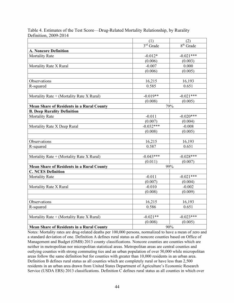
44
Table 4. Estimates of the Test Score—Drug-Related Mortality Relationship, by Rurality Definition, 2009-2014 (1) (2) 3rd Grade 8th Grade A. Noncore Definition Mortality Rate -0.012* -0.021*** (0.006) (0.003) Mortality Rate X Rural -0.007 0.000 (0.006) (0.005) Observations 16,215 16,193 R-squared 0.585 0.651 Mortality Rate + (Mortality Rate X Rural) -0.019** -0.021*** (0.008) (0.005) Mean Share of Residents in a Rural County 79% B. Deep Rurality Definition Mortality Rate -0.011 -0.020*** (0.007) (0.004) Mortality Rate X Deep Rural -0.032*** -0.008 (0.008) (0.005) Observations 16,215 16,193 R-squared 0.587 0.651 Mortality Rate + (Mortality Rate X Rural) -0.043*** -0.028*** (0.011) (0.007) Mean Share of Residents in a Rural County 99% C. NCES Definition Mortality Rate -0.011 -0.021*** (0.007) (0.004) Mortality Rate X Rural -0.010 -0.002 (0.008) (0.009) Observations 16,215 16,193 R-squared 0.586 0.651 Mortality Rate + (Mortality Rate X Rural) -0.021** -0.023*** (0.008) (0.005) Mean Share of Residents in a Rural County 90%
Notes: Mortality rates are drug-related deaths per 100,000 persons, normalized to have a mean of zero and a standard deviation of one. Definition A defines rural status as all noncore counties based on Office of Management and Budget (OMB) 2013 county classifications. Noncore counties are counties which are neither in metropolitan nor micropolitan statistical areas. Metropolitan areas are central counties and outlying counties with strong commuting ties and an urban population of over 50,000 while micropolitan areas follow the same definition but for counties with greater than 10,000 residents in an urban area. Definition B defines rural status as all counties which are completely rural or have less than 2,500 residents in an urban area drawn from United States Department of Agriculture’s Economic Research Service (USDA ERS) 2013 classifications. Definition C defines rural status as all counties in which over

45
75% of students attend a school classified as rural based on National Center for Education Statistics (NCES) 2010-2011 school year classifications. Mean Share of Residents in a Rural County is the mean share of residents in a county classified as rural for each definition of rurality, drawn from the 2010 Census. Results in each panel and column are from separate estimates. Linear combinations are included below point estimates in each panel. All estimates include state and year fixed effects, and county-level education, demographic, and economic controls. Parameter estimates for covariates not displayed. Standard errors clustered by state; *** p<0.01, ** p<0.05, * p<0.1
46
Appendix A: Data
Since there is no comprehensive measure for opioid use or educational outcomes, we
have collected data national county-level opioid measures and educational outcomes from
numerous sources. Our education dataset beings in 2009 while the most recently available opioid
morality data extends to 2014, which provides us with 2009-2014 as our period of analysis. This
covers parts of all three waves of the opioid crisis, with first years coinciding with the transition
between prescription opioids and heroin and the last year capturing the beginning of the rise in
overdoses caused by synthetic opioids.
Working at the county level allows us the greatest ability to link the disparate data
sources that we employ for the study. The county level also provides us with a unit of analysis
that for the most part exists nationally, which facilitates cross-region comparison. We miss out
on some level of variation by aggregating to the county level, as there may be differential effects
in more granular units of analysis such as school catchment zone. Populous counties may be
particularly affected, future research may use alternative measures which capture this variation.
Furthermore, school district boundaries may cross multiple counties which may introduce some
level of measurement error. This may be less of an issue for our results on rural counties, as they
may be more likely to have populations relatively fixed within county borders.
Opioid Data
Our primary measure of opioid use is drug-related overdose mortality rates as based on death
record data from the Centers for Disease Control and Prevention (CDC). Because of small-cell
reporting limitations, potential underreporting of drug overdoses, and ambiguity or
misspecification in underlying death certificate codes, we use data from the Institute for Health
Metrics and Evaluation (IHME) which produces estimates of mortality rates for substance use

47
disorders and intentional injuries for each county and year, using de-identified death record data
from the CDC, Census population counts, and small area Bayesian estimation models. While the
IHME data do not represent exact numbers of opioid-related deaths by county, they offer the best
approximations allowing comparison across counties and years. One important factor supporting
the use of imputed data is “the existence of ‘garbage codes’ – insufficiently specific or
implausible cause of death codes … that may lead to misleading geographic or temporal
patterns” (Dwyer-Lindgren et al., 2018). As we are specifically examining geographic patterns it
is important for our model to account for these codes. The IHME data provide mortality rate
estimates for every county in the United States for every year from 1980 to 2014. With these
data we average morality rates over the approximate lifetime of the student, 9 years for 3rd
graders and 14 years for 8th graders, which allows us to capture the cumulative effect of their
lifetime exposure to the opioid crisis. As opioids account for around the majority of drug-related
overdoses this measure serves to capture the relative intensity of the opioid crisis.
Education Data
The primary data source for educational outcomes comes from the Stanford Educational
Data Archive (SEDA). SEDA data contain academic performance metrics, measured through
standardized test scores that are re-scaled and standardized, county in the United States. Our
primary outcomes are math and English language arts (ELA) standardized test scores in grades 3
and 8. The SEDA data allows cross-county comparison of the relative test performance of 3rd and
8th grade students. As standardized test scores inherently reflect the totality of schooling (teacher
quality) and non-schooling (toxic stress response) factors over the course of a student’s lifetime
we include a variety of control variables in order to isolate the variation which is due to exposure
to opioid use.

48
Rurality Data
Our main specification uses Census defined percentage of county residents in a rural area
to define a rural county as one in which over 75% of the population resides in a rural area. Our
second measure uses the 2013 OMB designation of noncore counties to signify rural status.
Noncore counties are counties which are neither in metropolitan nor micropolitan statistical
areas. Metropolitan areas are central counties and outlying counties with strong commuting ties
and an urban population of over 50,000 while micropolitan areas follow the same definition but
for counties with greater than 10,000 residents in an urban area. The NCHS considers noncore
counties to be the most rural (Ingram and Franco, 2014). Our third measure, deep rurality, uses
the 2013 rural-urban commuting area codes from the USDA’s Economic Research Service. We
define deeply rural counties as those counties which are “completely rural or less than 2,500
urban population” (USDA, 2019). Our final measure of rurality uses 2010-2011 school year data
from NCES. These data classify schools as urban, suburban, town, or rural and we define a
county as rural if over 75% of the total student population attends a school classified as rural.
Student enrollment data are based on enrollment as of October 2010.
Covariates
We have three categories of control variables – district-level education controls, county-
level demographic controls, and county-level economic controls. Education controls are district-
level school characteristic and demographic measures from the SEDA dataset. We include
percent black and percent Hispanic/Latino in 3rd or 8th grade, school level percentages of English
language learners and special education students, and county-level measures of total schools,
total charter schools, pupil-teacher ratio, and expenditures per pupil.

49
County-level demographic controls are percentages measuring residents which are
foreign born, single parents, non-white, rural residents, holders of a bachelor’s degree or higher,
and in poverty. Additionally, we control for median household income, population density, total
population, and total land area. County-level controls are drawn from the Opportunity Insights
dataset and the 2010 Census. The timeframe we analyze is short enough that static measures in
2010 ought to be representative enough of the timeframe to be comparable across counties. Our
county-level economic indicators are the unemployment rate, annualized job growth between
2004 and 2013, and job density in 2013.

50
Appendix B: Supplemental Figures and Tables Appendix Table B1: Data Summary Statistics
Mean Std Dev A. Test Scores 3rd Grade Math & ELA 0.02 0.28 8th Grade Math & ELA -0.09 0.28 B. Opioid Measures Drug-Related Death Rates 9-yr lag (3rd Grade) 7.44 4.22 Drug-Related Death Rates 14-yr lag (8th Grade) 6.07 3.45 C. K-12 Education Measures
% Black 3rd Grade 0.12 0.20
% Black 8th Grade 0.12 0.20
% Hispanic 3rd Grade 0.11 0.17
% Hispanic 8th Grade 0.10 0.16 % ELL 0.04 0.06 % Special Ed 0.14 0.04 # of schools 12.74 39.30 # of charter schools 0.76 5.23 Pupil-teacher ratio 14.88 2.84 Expenditures per pupil 11,687 3,373 D. County Demographic Measures
% BA+ 2010 0.19 0.08 % Foreign born 2010 0.04 0.05 Median HH Inc 2016 48,520 13,128 % Poverty 2010 0.16 0.06 % Single parents 2010 0.31 0.09 % Non-white 2010 0.21 0.20 Population density 2010 219.54 1,383.21 Total population 2010 94,248.73 299,634.37 Total area (millions sq. meters) 2010 2800 9640 % rural population 2010 58.90 30.99 E. County Economic Measures
Unemployment rate 8.15 3.04 Annualized job growth 2004-13 0.00 0.01 Job density 104.61 714.62
Notes: All measures at a county level. Drug-related Death Rates are per 100,000 persons. Sample Size: 17,093 Source: Education data are from the Stanford Educational Data Archive (SEDA). Mortality data are from the Institute for Health Metrics and Evaluation. Demographic and economic data are from the 2010 Census and the Opportunity Insights dataset.

51
Appendix Table B2: Data Summary Statistics by Rurality Nonrural Rural Mean Std Dev Mean Std Dev A. Test Scores 3rd Grade Math & ELA 0.03* 0.27 -0.01* 0.31 8th Grade Math & ELA -0.08* 0.27 -0.12* 0.30 B. Opioid Measures Drug-Related Death Rates 9-yr lag (3rd Grade) 7.57* 3.94 7.17* 4.72 Drug-Related Death Rates 14-yr lag (8th Grade)
6.19* 3.26 5.82* 3.78
C. K-12 Education Measures % Black 3rd Grade 12.89* 19.10 10.22* 20.87 % Black 8th Grade 13.37* 19.68 10.55* 21.43 % Hispanic 3rd Grade 13.72* 18.41 6.66* 11.79 % Hispanic 8th Grade 12.40* 17.90 5.80* 11.02 % ELL 4.28* 6.44 2.09* 4.60 % Special Ed 13.51* 3.48 14.07* 4.09 # of schools 16.81* 47.65 4.70* 3.39 # of charter schools 1.12* 6.39 0.06* 0.29 Pupil-teacher ratio 15.42* 2.67 13.81* 2.87 Expenditures per pupil 11,481* 3,154 12,093* 3,736 D. County Demographic Measures % BA+ 2010 20.43* 8.92 14.92* 5.23 % Foreign born 2010 5.12* 5.73 2.23* 4.14 Median HH Inc 2016 50,938* 13,971 43,744* 9,638 % Poverty 2010 15.39* 6.26 16.40* 6.58 % Single parents 2010 31.56* 8.29 29.05* 9.92 % Non-white 2010 23.77* 19.73 16.34* 18.49 Population density 2010 317* 1,689 28* 25 Total population 2010 134,639* 360,975 14,467* 12,526 Total area (millions sq. meters) 2010 2770 7380 2850 13,000 % rural population 2010 41.11* 21.59 94.04* 8.82 E. County Economic Measures Unemployment rate 8.11 2.85 8.10 3.46 % Annualized job growth 2004-13 -0.07* 1.35 -0.63* 1.56 Job density 182.14* 1,055.39 10.67* 10.57
Notes: All measures at a county level. In this table, a county is considered rural if at least 75% of residents live in a rural area drawn from the 2010 Census. Drug-related Death Rates are per 100,000 persons. Sample Size: Total = 17,093; Rural = 5,745 (34%); Nonrural = 11,348 (66%). * indicates means are statistically different at the 95% level. Source: Education data are from the Stanford Educational Data Archive (SEDA). Mortality data are from the Institute for Health Metrics and Evaluation. Demographic and economic data are from the 2010 Census and the Opportunity Insights dataset.

52
Appendix Table B3: Average drug-related mortalities per 100,000 persons per decile, 3rd Grade Decile Mean A. 3rd Grade 1st Decile 2.61 2nd Decile 3.75 3rd Decile 4.60 4th Decile 5.35 5th Decile 6.10 6th Decile 6.94 7th Decile 7.95 8th Decile 9.23 9th Decile 11.17 10th Decile 16.69 B. 8th Grade 1st Decile 2.13 2nd Decile 3.05 3rd Decile 3.74 4th Decile 4.35 5th Decile 4.98 6th Decile 5.5 7th Decile 6.48 8th Decile 7.54 9th Decile 9.19 10th Decile 13.80
Notes: Average drug-related mortality for 3rd grade is the average for the 9 years preceding the observation year. For a 3rd grade student in 2009 this is the average between 2000 and 2008. Average drug-related mortality for 8th grade is the average for the 14 years preceding the observation year. For an 8th grade student in 2009 this is the average between 1995 and 2008. Source: Institute for Health Metrics and Evaluation.
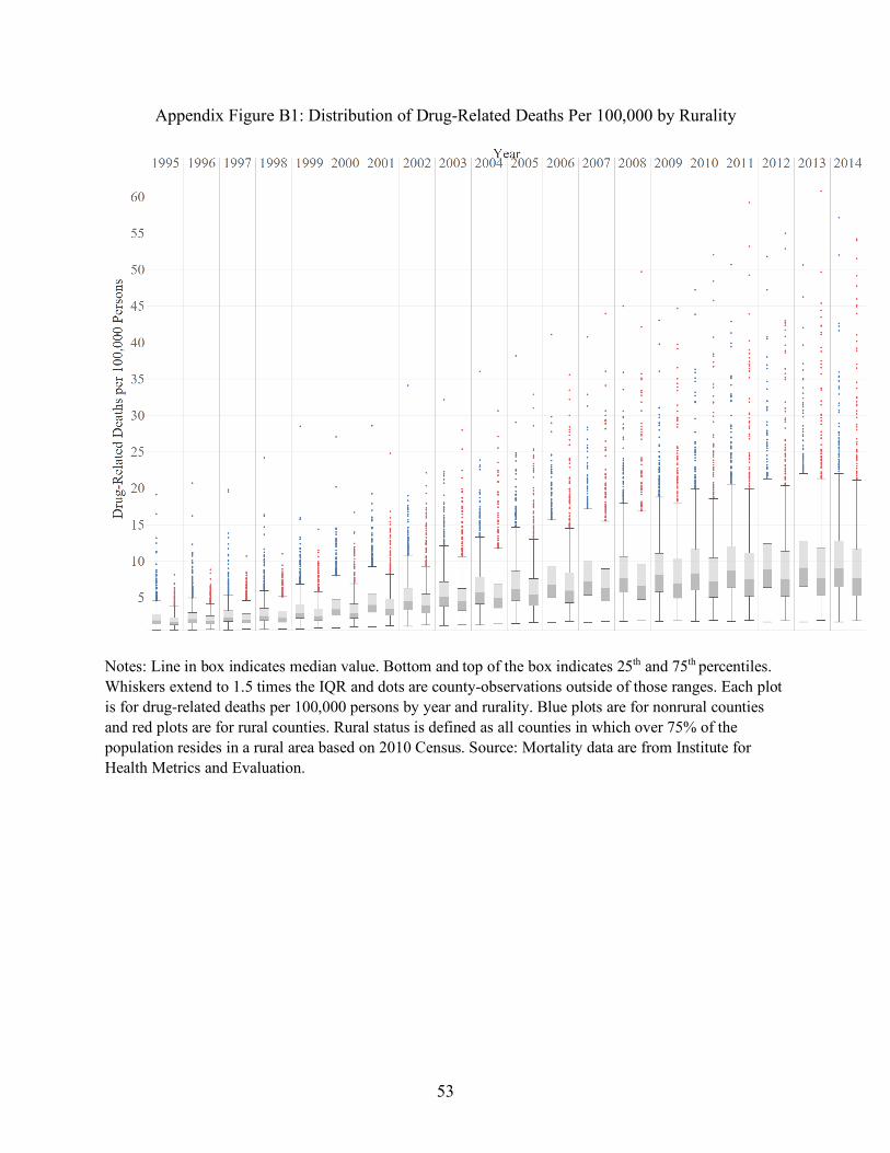
53
Appendix Figure B1: Distribution of Drug-Related Deaths Per 100,000 by Rurality
Notes: Line in box indicates median value. Bottom and top of the box indicates 25th and 75th percentiles. Whiskers extend to 1.5 times the IQR and dots are county-observations outside of those ranges. Each plot is for drug-related deaths per 100,000 persons by year and rurality. Blue plots are for nonrural counties and red plots are for rural counties. Rural status is defined as all counties in which over 75% of the population resides in a rural area based on 2010 Census. Source: Mortality data are from Institute for Health Metrics and Evaluation.

54
Appendix Figure B2: Distribution of Drug-Related Deaths Per 100,000 by Rurality
(A) 3rd Grade
(B) 8th Grade
Notes: Dividing line in box indicates median value. Bottom and top of the box indicates 25th and 75th
percentiles. Whiskers extend to 1.5 times the IQR and dots are county-observations outside of those ranges. Drug-related deaths per 100,000 persons are the average for the 9 years prior to the observation year for 3rd graders and 14 years prior to the observation year for eighth graders (e.g. for a student in 3rd grade in 2009 this measure captures the drug-related deaths over the course of the lifetime 2000-2008). Observation years are 2009-2014. Source: Institute for Health Metrics and Evaluation.

55
Appendix C: Alternative Definitions of Rurality
Appendix Figure C1: Maps of the United States using various definitions of rurality
(A) Over 75% of County Residents in Rural Area
(B) Noncore Definition of Rural Counties

56
(C) Deep Rural Counties based on ERS Definitions
(D) Over 75% of Students Attend Rural District based on NCES
Notes: Definition A defines rural status as all counties in which over 75% of the population resides in a rural area based on 2010 Census designation of rural status. Definition B defines rural status as all noncore counties based on Office of Management and Budget (OMB) 2013 county classifications. Noncore counties are counties which are neither in metropolitan nor micropolitan statistical areas. Metropolitan areas are central counties and outlying counties with strong commuting ties and an urban population of over 50,000 while micropolitan areas follow the same definition but for counties with greater than 10,000 residents in an urban area. Definition C defines rural status as all counties which are completely rural or have less than 2,500 residents in an urban area drawn from United States Department of Agriculture’s Economic Research Service (USDA ERS) 2013 classifications. Definition D defines rural status as all counties in which over 75% of students attend a school classified as rural based on National Center for Education Statistics (NCES) 2010-2011 school year classifications (data gathered October 2010). Number of counties by each definition: (A) Rural = 1,063, Nonrural = 2,079; (B) - Rural = 1,335, Nonrural = 1,807; (C) – Rural = 643, Nonrural = 2,497; (D) – Rural = 1,072, Nonrural = 2,065. Due to missing counties in certain datasets the number of counties by each measure ranges from 3,442 for our main specification to 4,337 under the NCES definition.
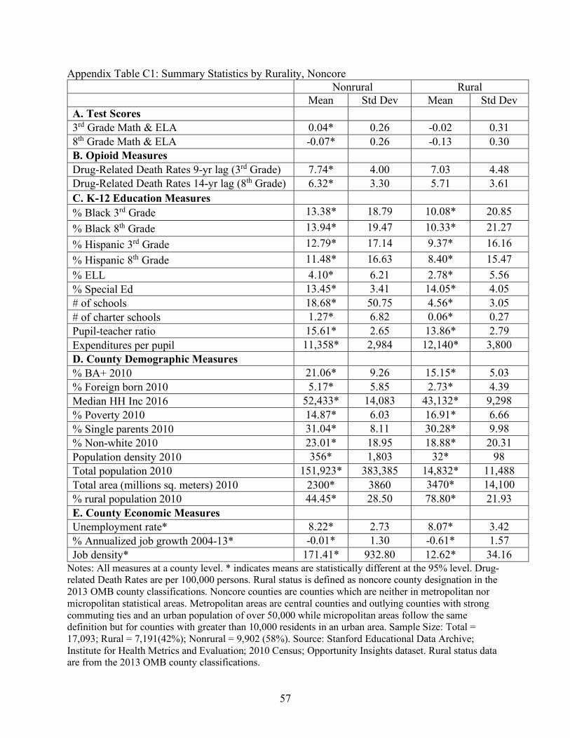
57
Appendix Table C1: Summary Statistics by Rurality, Noncore Nonrural Rural Mean Std Dev Mean Std Dev A. Test Scores 3rd Grade Math & ELA 0.04* 0.26 -0.02 0.31 8th Grade Math & ELA -0.07* 0.26 -0.13 0.30 B. Opioid Measures Drug-Related Death Rates 9-yr lag (3rd Grade) 7.74* 4.00 7.03 4.48 Drug-Related Death Rates 14-yr lag (8th Grade) 6.32* 3.30 5.71 3.61 C. K-12 Education Measures % Black 3rd Grade 13.38* 18.79 10.08* 20.85 % Black 8th Grade 13.94* 19.47 10.33* 21.27 % Hispanic 3rd Grade 12.79* 17.14 9.37* 16.16 % Hispanic 8th Grade 11.48* 16.63 8.40* 15.47 % ELL 4.10* 6.21 2.78* 5.56 % Special Ed 13.45* 3.41 14.05* 4.05 # of schools 18.68* 50.75 4.56* 3.05 # of charter schools 1.27* 6.82 0.06* 0.27 Pupil-teacher ratio 15.61* 2.65 13.86* 2.79 Expenditures per pupil 11,358* 2,984 12,140* 3,800 D. County Demographic Measures % BA+ 2010 21.06* 9.26 15.15* 5.03 % Foreign born 2010 5.17* 5.85 2.73* 4.39 Median HH Inc 2016 52,433* 14,083 43,132* 9,298 % Poverty 2010 14.87* 6.03 16.91* 6.66 % Single parents 2010 31.04* 8.11 30.28* 9.98 % Non-white 2010 23.01* 18.95 18.88* 20.31 Population density 2010 356* 1,803 32* 98 Total population 2010 151,923* 383,385 14,832* 11,488 Total area (millions sq. meters) 2010 2300* 3860 3470* 14,100 % rural population 2010 44.45* 28.50 78.80* 21.93 E. County Economic Measures Unemployment rate* 8.22* 2.73 8.07* 3.42 % Annualized job growth 2004-13* -0.01* 1.30 -0.61* 1.57 Job density* 171.41* 932.80 12.62* 34.16
Notes: All measures at a county level. * indicates means are statistically different at the 95% level. Drug-related Death Rates are per 100,000 persons. Rural status is defined as noncore county designation in the 2013 OMB county classifications. Noncore counties are counties which are neither in metropolitan nor micropolitan statistical areas. Metropolitan areas are central counties and outlying counties with strong commuting ties and an urban population of over 50,000 while micropolitan areas follow the same definition but for counties with greater than 10,000 residents in an urban area. Sample Size: Total = 17,093; Rural = 7,191(42%); Nonrural = 9,902 (58%). Source: Stanford Educational Data Archive; Institute for Health Metrics and Evaluation; 2010 Census; Opportunity Insights dataset. Rural status data are from the 2013 OMB county classifications.
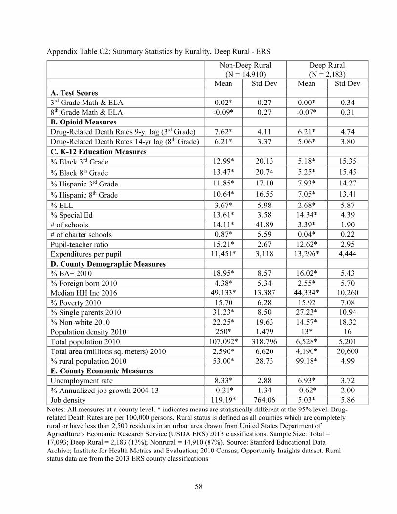
58
Appendix Table C2: Summary Statistics by Rurality, Deep Rural - ERS
Non-Deep Rural
(N = 14,910) Deep Rural (N = 2,183)
Mean Std Dev Mean Std Dev A. Test Scores 3rd Grade Math & ELA 0.02* 0.27 0.00* 0.34 8th Grade Math & ELA -0.09* 0.27 -0.07* 0.31 B. Opioid Measures Drug-Related Death Rates 9-yr lag (3rd Grade) 7.62* 4.11 6.21* 4.74 Drug-Related Death Rates 14-yr lag (8th Grade) 6.21* 3.37 5.06* 3.80 C. K-12 Education Measures % Black 3rd Grade 12.99* 20.13 5.18* 15.35 % Black 8th Grade 13.47* 20.74 5.25* 15.45 % Hispanic 3rd Grade 11.85* 17.10 7.93* 14.27 % Hispanic 8th Grade 10.64* 16.55 7.05* 13.41 % ELL 3.67* 5.98 2.68* 5.87 % Special Ed 13.61* 3.58 14.34* 4.39 # of schools 14.11* 41.89 3.39* 1.90 # of charter schools 0.87* 5.59 0.04* 0.22 Pupil-teacher ratio 15.21* 2.67 12.62* 2.95 Expenditures per pupil 11,451* 3,118 13,296* 4,444 D. County Demographic Measures % BA+ 2010 18.95* 8.57 16.02* 5.43 % Foreign born 2010 4.38* 5.34 2.55* 5.70 Median HH Inc 2016 49,133* 13,387 44,334* 10,260 % Poverty 2010 15.70 6.28 15.92 7.08 % Single parents 2010 31.23* 8.50 27.23* 10.94 % Non-white 2010 22.25* 19.63 14.57* 18.32 Population density 2010 250* 1,479 13* 16 Total population 2010 107,092* 318,796 6,528* 5,201 Total area (millions sq. meters) 2010 2,590* 6,620 4,190* 20,600 % rural population 2010 53.00* 28.73 99.18* 4.99 E. County Economic Measures Unemployment rate 8.33* 2.88 6.93* 3.72 % Annualized job growth 2004-13 -0.21* 1.34 -0.62* 2.00 Job density 119.19* 764.06 5.03* 5.86
Notes: All measures at a county level. * indicates means are statistically different at the 95% level. Drug-related Death Rates are per 100,000 persons. Rural status is defined as all counties which are completely rural or have less than 2,500 residents in an urban area drawn from United States Department of Agriculture’s Economic Research Service (USDA ERS) 2013 classifications. Sample Size: Total = 17,093; Deep Rural = 2,183 (13%); Nonrural = 14,910 (87%). Source: Stanford Educational Data Archive; Institute for Health Metrics and Evaluation; 2010 Census; Opportunity Insights dataset. Rural status data are from the 2013 ERS county classifications.

59
Appendix Table C3: Summary Statistics by Rurality, Over 75% Students Attend a Rural School - NCES Nonrural Rural Mean Std Dev Mean Std Dev A. Test Scores 3rd Grade Math & ELA 0.02* 0.27 0.00* 0.31 8th Grade Math & ELA -0.08* 0.27 -0.11* 0.30 B. Opioid Measures Drug-Related Death Rates 9-yr lag (3rd Grade) 7.65* 3.97 7.04* 4.65 Drug-Related Death Rates 14-yr lag (8th Grade) 6.25* 3.28 5.71* 3.73 C. K-12 Education Measures % Black 3rd Grade 12.87* 19.36 10.30* 20.39 % Black 8th Grade 13.34* 19.93 10.65* 20.96 % Hispanic 3rd Grade 13.50* 18.44 7.18* 12.07
% Hispanic 8th Grade 12.20* 17.92 6.27* 11.31 % ELL 4.15* 6.25 2.38* 5.22 % Special Ed 13.57* 3.48 13.96* 4.10 # of schools 16.80* 47.81 4.87* 3.70 # of charter schools 1.12* 6.41 0.07* 0.32 Pupil-teacher ratio 15.42* 2.63 13.82* 2.95 Expenditures per pupil 11,467* 3,078 12,112* 3,847 D. County Demographic Measures % BA+ 2010 20.24* 8.93 15.34* 5.63 % Foreign born 2010 5.06* 5.87 2.38* 3.84 Median HH Inc 2016 50,583* 13,963 44,523* 10,214 % Poverty 2010 15.45* 6.17 16.26* 6.75 % Single parents 2010 31.61* 08.20 28.99* 10.03 % Non-white 2010 23.41* 19.70 17.12* 18.83 Population density 2010 316* 1,695 32* 36 Total population 2010 134,879* 362,097 15,551* 18,356 Total area (millions sq. meters) 2010 2,740* 6,950 2,900* 13,400 % rural population 2010 42.80* 23.80 90.09* 15.80 E. County Economic Measures Unemployment rate 8.20* 2.84 8.07* 3.40 % Annualized job growth 2004-13 -0.11* 1.32 -0.56* 1.62 Job density 151.79* 876.17 13.21* 16.42
Notes: All measures at a county level. * indicates means are statistically different at the 95% level. Drug-related Death Rates are per 100,000 persons. Rural status is defined as a county where >75% of students attend a school designated as rural for the 2010-2011 academic year (data gathered October 2010). Data on membership based on school membership as of October 2010. Sample Size: Total = 17,093; Rural = 5,820 (34%); Nonrural = 11,273 (66%). Source: Stanford Educational Data Archive; Institute for Health Metrics and Evaluation; 2010 Census; Opportunity Insights dataset. Rural status data are from the 2010-2011 school year NCES school classifications.