1

The Optimality of Being Efficient Lawrence M. Ausubel and Peter Cramton*

University of Maryland

18 June 1999

Abstract

In an optimal auction, a revenue-optimizing seller often awards goods inefficiently, either by

placing them in the wrong hands or by withholding goods from the market. This conclusion

rests on two assumptions: (1) the seller can prevent resale among bidders after the auction; and

(2) the seller can commit to not sell the withheld goods after the auction. We examine how the

optimal auction problem changes when these assumptions are relaxed. In sharp contrast to the

no resale assumption, we assume perfect resale: all gains from trade are exhausted in resale. In a

multiple object model with independent signals, we characterize optimal auctions with resale.

We prove generally that with perfect resale, the seller’s incentive to misassign goods is

destroyed. Moreover, with discrete types, any misassignment of goods strictly lowers the

seller’s revenue from the optimum. In auction markets followed by perfect resale, it is optimal

to assign goods to those with the highest values.

JEL No.: D44 (Auctions) Keywords: Auctions, Multiple Object Auctions, Resale Send comments to: Professors Lawrence M. Ausubel or Peter Cramton Department of Economics University of Maryland College Park, MD 20742-7211 ausubel@econ.umd.edu cramton@umd.edu (301) 405-3495 (301) 405-6987 *The authors gratefully acknowledge the support of the National Science Foundation and the World Bank. We thank Susan Athey, Milton Harris, John Riley, Valter Sorana, S. Viswanathan, Robert Wilson, and seminar participants at the Maryland Auction Conference, the Econometric Society Summer Meetings, the Utah Winter Finance Conference, and the Society of Financial Studies Conference on Price Formation for helpful comments.

2

The Optimality of Being Efficient Lawrence M. Ausubel and Peter Cramton

1 Introduction A cornerstone of the auction literature is the theory of “optimal auctions.”1 This theory uses

mechanism design techniques to characterize, in general settings, the auction that maximizes the seller’s

expected revenues. One feature of the solution is that typically there is a conflict between the goals of

revenue maximization and efficiency. The revenue-optimizing seller often either misassigns goods

(placing them in hands other than those who value them the most) or withholds goods (restricting the

quantity brought to market). However, the conclusion that the seller gains by misassigning and

withholding goods depends critically on two strong assumptions: (1) the seller can prevent resale among

bidders from occurring after the auction; and (2) the seller can commit to not sell the withheld goods after

the auction. In this paper, we examine how the optimal auction problem changes when one or both of

these assumptions are relaxed.

When the seller cannot ban resale, the bidders may undo the seller’s misassignment. If agents

understand and anticipate this, the incentives that the seller attempted to create in the solution to the

mechanism design problem are undermined, and so the “optimal” auction may cease to be optimal. Coase

(1960) has criticized standard economic analyses of the law that assume away the possibility that

economic agents may recognize any gains from trade, by instead making the opposite extreme assumption

that all gains from trade are realized. For most of this paper, we will adopt the Coase Theorem by

assuming perfect resale. Resale causes any misassignment of the goods to be corrected. This is an extreme

assumption. Certainly, there are settings where perfect resale is not possible, because of private

information that the auction winners have after the auction (Myerson and Satterthwaite 1983; Cramton,

Gibbons and Klemperer 1987). However, there are other settings where perfect resale is possible. One

way to guarantee that perfect resale is possible is to assume that all private information is publicly

revealed after the auction. We do not make this assumption. Private information is publicly revealed only

through the bidders’ actions in the auction game and the resale game.2

1 This research began with Myerson (1981) and has since been extended by many others, for example, Engelbrecht-Wiggans (1988), Cremer and McLean (1985, 1988), Maskin and Riley (1989), McAfee and Reny (1992), and Bulow and Klemperer (1996). 2 If private information is revealed “for free” following the auction, then the optimal auction is for the seller to retain all goods in the auction, wait for all information to be revealed, and finally make take-it-or-leave-it offers to the efficient recipients at their reservation values.

3

Perfect resale has the significant advantage that it is a simple and general assumption on the resale

market. Moreover, since resale is voluntary, resale inevitable shifts outcomes toward the efficient

assignment. The disadvantage of our assumption is that it is an assumption on the outcome of the resale

game, rather than on the rules of the game. In addition, perfect resale may not be attainable in some

situations. Still, we view perfect resale as a tractable first approximation of many resale markets.

When the seller cannot commit to refrain from selling the withheld objects after the auction, the

seller may himself undo the inefficient allocation of the auction. Again, if agents understand and

anticipate this, the “optimal” auction may cease to be optimal. Coase (1972) has criticized standard

economic analyses of durable goods monopoly that assume the seller has full commitment powers, by

instead making the opposite extreme assumption that the seller has no commitment powers. In parts of

this paper, we will take the Coase Conjecture seriously and explore the implications of no commitment

powers by the seller. Without commitment, all inefficient withholding of the goods is corrected. Again,

this is an extreme assumption. Certainly, there are reasons why the seller may credibly withhold goods

from the market for long periods of time (Ausubel and Deneckere 1989). That said, the Coase Conjecture

remains a simple assumption on post-auction behavior whose implications are certainly worth exploring,

and may at least be an acceptable assumption for modeling real-world situations where the seller chooses

not to utilize any reserve price.

Armed with the Coasean assumptions, we state and solve three auction programs:

1. Unconstrained auction program. The seller can forbid resale and commit to not selling

additional goods after the auction. Hence, the seller maximizes revenues, under the hypothesis

that resale among buyers is impossible.

2. Resale-constrained auction program. The seller can withhold supply, but cannot prevent resale.

Thus, the seller maximizes revenues, subject to the constraint that there will be perfect resale

among bidders after the auction.

3. Efficiency-constrained auction program. The seller can neither withhold supply, nor prevent

resale. Hence, the seller maximizes revenues, subject to the constraint that there will be perfect

resale among the seller and bidders after the auction.

We analyze an “independent signals” model with multiple identical objects. Each risk-neutral bidder has a

private signal about its demand for the good. A bidder’s demand may depend on all bidders’ signals, and

the signals are assumed independent. This model includes both private value and common value models

as special cases. It allows ex ante asymmetries among bidders.

4

Each of the auction programs is solved via a general version of the Revenue Equivalence Theorem:

Any auction that results in the same assignment of the goods yields the same seller revenues, provided

that the lowest bidder types get the same payoff. Moreover, when the lowest bidder types are given zero

surplus (as they are in any optimal auction), this revenue equals the marginal revenues integrated over the

quantity won and summed over bidders. Marginal revenue is what the seller gets from awarding

additional quantity to a bidder. It is equal to the bidder’s marginal value less the informational rent that

the bidder is able to capture from its private information.

In the unconstrained auction program, the seller simply assigns the good in descending order of

marginal revenue, until the good is exhausted or marginal revenue turns negative. Goods are assigned by

moving down the aggregate marginal revenue curve.

In the efficiency-constrained auction program, the seller is forced to assign the goods efficiently. The

seller’s only discretion occurs when there is a tie in marginal values (the aggregate demand curve is flat).

Then the seller assigns first to those with the higher marginal revenue. Goods are assigned by moving

down the aggregate demand curve, until the quantity available is exhausted.

In the resale-constrained auction program, the seller has more discretion. Because of perfect resale,

the seller is forced to award in descending order of marginal value (i.e., by moving down the aggregate

demand curve), but the seller can withhold quantity. The seller’s choice of aggregate quantity depends on

the bidders’ reports of private information. The choice is complicated by the constraint that the aggregate

quantity must be weakly increasing in the bidders’ reports. Otherwise, a bidder may profitably deviate by

underreporting, to increase the quantity awarded, and then purchase some of this extra quantity in the

resale market. The inability to misassign the good typically results in more withholding than in the

unconstrained auction.

We show that, when a seller cannot prevent resale, the seller’s revenues can be no more than in the

resale-constrained auction program. The key to the argument is that any equilibrium of the auction-plus-

resale game must satisfy all the constraints of the resale-constrained auction program. Thus, an

equilibrium of the two-stage game cannot result in greater revenues. We then show that the seller can

achieve this upper bound in the auction-plus-resale game by using a Vickrey auction with reserve

pricing.3 In equilibrium, goods are assigned efficiently and resale does not occur, although quantity may

be withheld. If the seller cannot commit to withholding quantity, then the seller’s revenues can be no

3 Krishna and Perry (1997) show that in a market without resale the Vickrey auction implements the efficiency-constrained optimal auction, when the lowest types get 0. Our result allows for both resale and withholding of the good.

5

more than in the efficiency-constrained auction program. This upper bound also is attained by the Vickrey

auction with reserve pricing.

We next consider whether misassignment actually hurts the seller. Does the seller necessarily get

strictly lower revenues by any misassignment of the good? We show that the answer is yes in the identical

objects model with discrete types. The seller does strictly better by assigning the goods to those with the

highest values. Intuitively, misassigning the goods results in the seller foregoing a share of the gains from

trade that are ultimately captured by the bidders in resale.

Our results thus provide a new defense for emphasizing efficient auction design rather than “optimal”

auction design.4 The presence of a perfect resale market forces even the most selfish seller, whose sole

objective is maximizing revenues, to focus—out of necessity—on efficiency. While the Coasean

assumption of perfect resale is admittedly extreme, it still may better approximate outcomes in many

markets than the standard assumption of no resale which the auction literature routinely makes.

In this paper, we focus on the Coasean critiques of the optimal auction program. Other critiques

strengthen our conclusion. For example, when one recognizes that bidder participation is affected by the

auction design, then the case for an efficient auction improves. McAfee and McMillan (1987), Harstad

(1990, 1993), and Levin and Smith (1994, 1995, 1996) provide justification why a revenue-maximizing

seller should care about efficiency. With endogenous bidder participation and symmetric bidders,

efficiency and revenue-maximization are equivalent. Bulow and Klemperer (1996) demonstrate that if a

reserve price discourages even a single potential bidder from participating, the reserve makes the seller

worse off.

Another critique of the optimal auction approach is the severe informational requirement placed on

the mechanism designer. The approach assumes that the distributions of private information are common

knowledge, and the optimal auction makes explicit use of this information. If the seller does not know the

distributions or is constrained to adopt auction rules that are independent of the distributions, then

implementing the optimal auction may be impossible (but see Caillaud and Robert, 1998). In contrast, the

informational requirements of the efficient auction are often less severe. In interesting cases, the efficient

auction rules may be independent of the distributions of private information (see, for example, Ausubel,

1997).

4 Recent papers emphasizing efficiency rather than revenue maximization as the seller’s objective include Ausubel (1997), Ausubel and Cramton (1998), Dasgupta and Maskin (1997), and Krishna and Perry (1997). The real-world discussion of how best to structure the FCC spectrum auctions tended also to emphasize efficiency over revenue maximization.

6

Our paper, by introducing a resale constraint into the optimal auction, is connected to both the resale

literature and the optimal auction literature. The study of resale in auction markets is just emerging.

Bikhchandani and Huang (1989) and Viswanathan and Wang (1996) develop models of Treasury

auctions, where resale is especially important. Bidding behavior is significantly affected by resale.

Agastya and Daripa (1998) also focus on Treasury auctions, emphasizing the interaction of the futures

market, the auction, and resale. Haile (1998), using a reduced-form representation of the resale market,

characterizes equilibrium bidding behavior in standard single-good auctions. Haile (1997) examines

resale in a setting where bidders acquire additional information after the auction. Haile (1996) empirically

tests the model using U.S. Forest Service timber data. Horstmann and LaCasse (1997) consider resale by

the seller to a potentially different set of bidders. Our paper is most closely related to several recent

studies of optimal auctions with multiple goods. For example, Krishna and Perry (1997) find conditions

under which the Vickrey auction is optimal among efficient mechanisms. Armstrong (1997) is also

interested in when an optimal auction is efficient. He shows that with two goods and two types, the

optimal auction is always efficient (this result, however, does not generalize to three types). Avery and

Hendershott (1998) analyze optimal bundling in a multiple objects setting.

Our paper is organized as follows. Section 2 illustrates our main results with three examples. In

section 3, we establish the seller’s general incentive to misassign goods, and we identify settings where

the optimal auction assigns goods efficiently. In section 4, we solve two variations on the optimal auction,

which recognize the possibility of resale. Section 5 proves that perfect resale destroys the seller’s

incentive to misassign goods. Section 6 establishes that, with perfect resale, any misassignment of goods

results in strictly lower seller revenues than the best efficient assignment. Section 7 concludes.

2 Three examples We begin with three examples. In each example, a seller is auctioning a single good to two bidders,

Strong and Weak. The bidders have independent private values. Strong has a higher expected value than

Weak. The seller’s value is commonly known to equal zero. The first and third examples have continuous

values; the second example has discrete values.

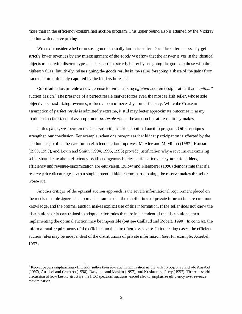
Example 1. Strong’s value is uniformly distributed between 0 and 10. Weak’s value is commonly

known to be 2. As summarized in Figure 1, any efficient auction assigns the good to Weak if Strong’s

value is less than 2, and otherwise assigns the good to Strong. In contrast, the “optimal” auction assigns

the good to Weak if Strong’s value is less than 6, and otherwise assigns the good to Strong, which is

inefficient whenever Strong’s value is between 2 and 6. This outcome is achieved by offering the good to

Strong at a price of 6, and otherwise selling the good to Weak at a price of 2. The seller sells at a price of

2 with probability .6 and sells at 6 with probability .4, yielding revenues of 2(.6) + 6(.4) = 3.6.

7

Figure 1. Alternative assignment rules (Weak’s value = 2) Efficient auction Weak Strong Optimal auction Weak Strong

Resale constrained None Strong Strong’s value 0 2 5 6 10

The intuition behind the misassignment in the optimal auction is that the seller finds it advantageous

to increase Strong’s incentive to make a high report, thereby enabling the seller to collect higher revenue

(than in the efficient auction) from Strong after a high report. The seller does this by withholding the good

from Strong whenever Strong makes a low report. Meanwhile, given that Weak always values the good

more than the seller, it is revenue-maximizing to assign the good to Weak whenever withholding it from

Strong.

The resale market undermines this outcome. Strong is unwilling to accept a price of 6, since Strong

does better by purchasing from Weak in the resale market. Perfect resale implies that Strong buys the

good from Weak whenever Strong’s value is greater than 2. This is accomplished by Strong offering a

take-it-or-leave-it offer of 2 to Weak. Hence, the “optimal auction” generates revenues of 2, which is the

same revenue generated by the efficient auction. This illustrates our main theorem that the seller cannot

enhance revenues by misassigning the good. The example also illustrates that the perfect resale

assumption imposes constraints on the resale game. In this case, perfect resale requires that Strong (the

bidder with private information) gets all the gains from trade in the resale game. Although extreme, this

assumption is consistent with the Coase Conjecture, which is often assumed in the bargaining literature.

The seller typically can do better by withholding the good; that is, setting a reserve that is sometimes

not met. In the resale-constrained auction program, the seller sets a reserve price of 5, which results in

revenues of .5(5) = 2.5. The seller forecloses the resale market by never assigning the good to Weak.

Notice that the seller is unable to assign the good to Weak even when Strong’s value is less than 2. Doing

so would give Strong an incentive to pretend to have a value that is less than 2, and then purchase the

good in the resale market at a price of 2.

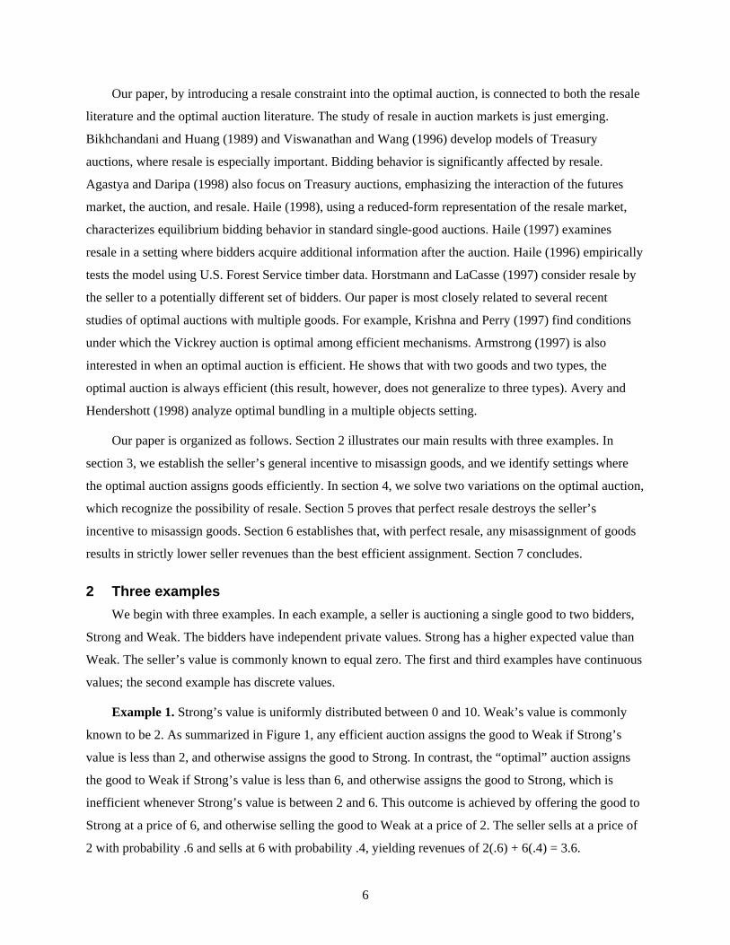
Example 2. Strong’s value is either H or M, and Weak’s value is either H or L, where H > M > L.

Strong’s value is high with probability s and Weak’s value is high with probability w. Efficiency requires

that Strong gets the good when Weak’s value is L. However, for an interesting region of parameters, the

“optimal” auction misassigns the good to Weak when Weak’s value is L and Strong’s value is M (see

Figure 2). This occurs whenever (1) the seller prefers a reserve price of H for Strong (sH ≥ M), and (2) the

seller prefers a reserve price of L for Weak (wH < L). Together these conditions imply that Strong’s

probability of H is greater than Weak’s (s > w). Then the seller offers the good to Strong at a price of H. If

8

Strong declines, the seller offers the good to Weak at L, which is surely accepted. Seller revenues are

sH + (1 − s)L.

Figure 2. Alternative assignment rules (Optimal / Efficient) Weak H L

H Either / Either Strong / Strong Strong M Weak / Weak Weak / Strong

As before, the intuition behind the misassignment in the optimal auction is that the seller finds it

advantageous to increase Strong’s incentive to report H, by withholding the good from Strong when

Strong reports M and Weak reports L. Meanwhile, in the interesting region of parameter values, it is

revenue-maximizing to assign the good to Weak whenever withholding it from Strong.

Again, resale undermines this outcome. If Weak gets the good and has a value of L, then Weak can

gain by reselling to Strong at a price of (M + L)/2. But this destroys Strong’s incentive to accept H. The

seller would end up with a revenue of L, since H is surely rejected by Strong, when resale is possible. If

instead of misassigning the good, the seller conducts an efficient (second-price) auction with reserve

prices of M for Strong and H for Weak, then the revenues are wH + (1 − w)M, which is greater than L.

Hence, the seller is made strictly worse off by misassigning the good. This illustrates Theorem 6.

If the seller can commit to withholding the good, the seller may do better by setting a reserve price of

H for both. This yields revenues of [1 − ( 1−s)(1−w)]H, which exceeds wH + (1 − w)M if M or w are

sufficiently small.

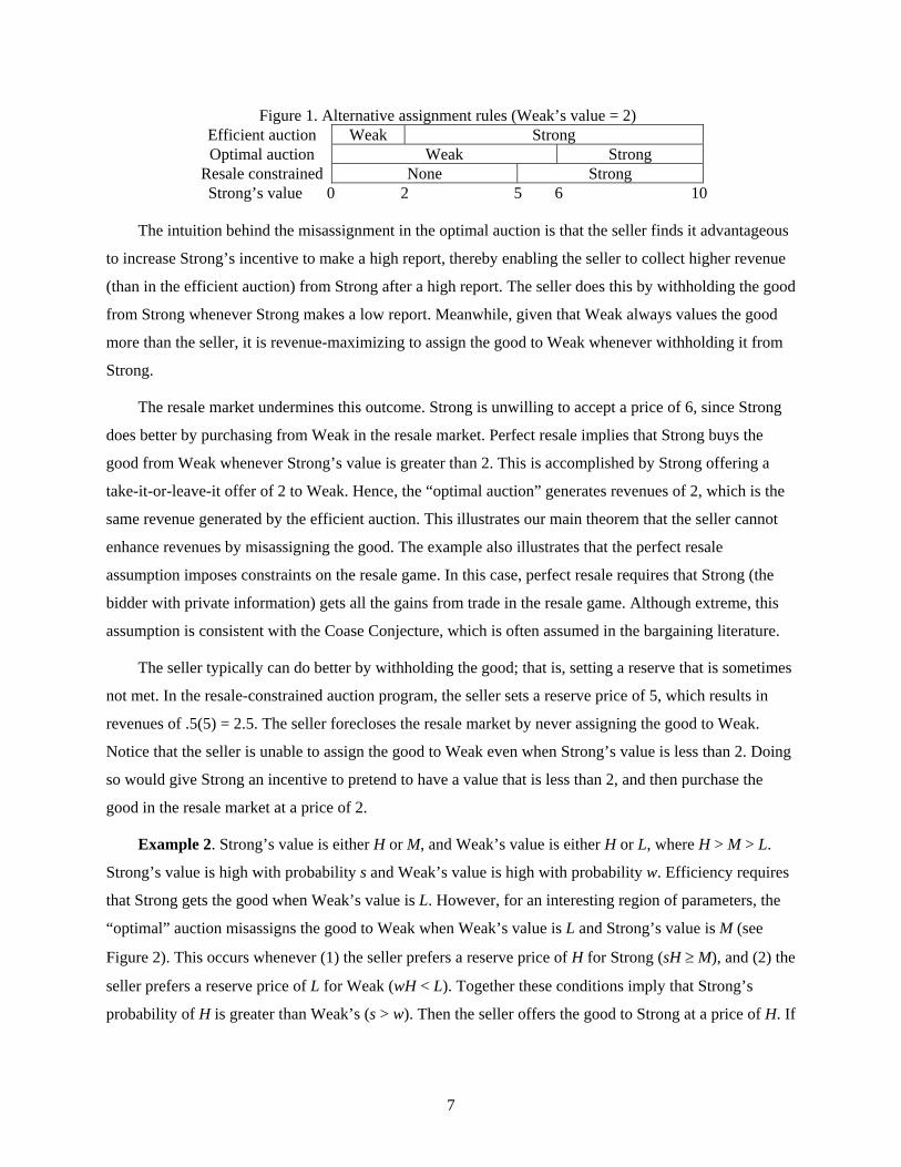
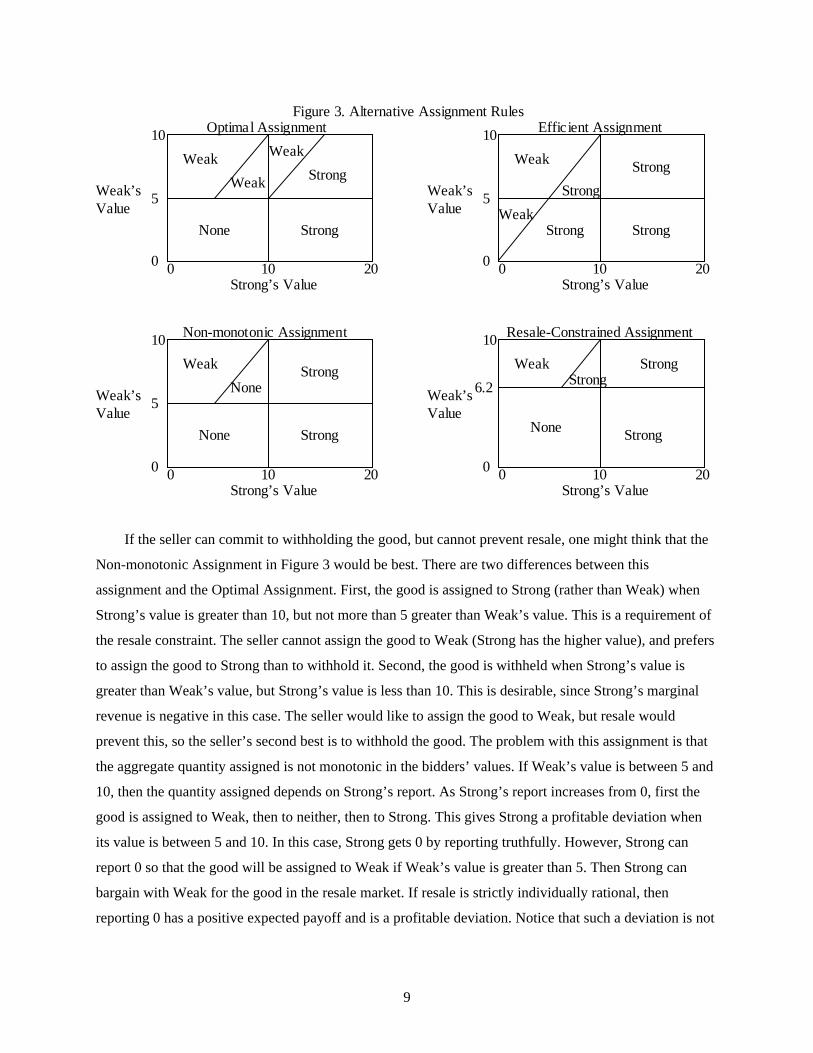
Example 3. Strong’s value s is uniformly distributed between 0 and 20. Weak’s value w is uniformly

distributed between 0 and 10. In the optimal auction, the seller assigns the good to the bidder with the

highest marginal revenue provided marginal revenue is positive. In this case, Strong’s marginal revenue is

MRs(s) = 2s – 20, and MRw(w) = 2w – 10. Hence, we set a reserve price of 10 for Strong, 5 for Weak, and

only sell to Strong if its value exceeds Weak’s value by at least 5 (s – w > 5), as shown in the Optimal

Assignment in Figure 3. The assignment includes both misassignment and withholding. Strong’s

incentive to report a high value is increased by the fact that the good is only assigned to Strong if its

report exceeds Weak’s report by at least 5. Moreover, at least one of the bidders must beat its reserve

price for the good to be assigned. In contrast, the Efficient Assignment always assigns the good, and

always to the bidder with the highest value.

9

10

0

5

0 10 20

Strong

Weak’s Value

None

Weak

Weak Strong

Strong’s Value

Weak

Optimal Assignment 10

0

5

0 10 20

Strong

Weak’s Value Weak

Strong

Strong’s Value

Weak

Efficient Assignment

10

0

5

0 10 20

Strong

Weak’s Value

Strong

Strong’s Value

Weak

Non-monotonic Assignment 10

0

6.2

0 10 20

Strong

Weak’s Value

Strong

Strong’s Value

Weak

Resale-Constrained Assignment

Strong

Strong

Strong

Figure 3. Alternative Assignment Rules

None

None None

If the seller can commit to withholding the good, but cannot prevent resale, one might think that the

Non-monotonic Assignment in Figure 3 would be best. There are two differences between this

assignment and the Optimal Assignment. First, the good is assigned to Strong (rather than Weak) when

Strong’s value is greater than 10, but not more than 5 greater than Weak’s value. This is a requirement of

the resale constraint. The seller cannot assign the good to Weak (Strong has the higher value), and prefers

to assign the good to Strong than to withhold it. Second, the good is withheld when Strong’s value is

greater than Weak’s value, but Strong’s value is less than 10. This is desirable, since Strong’s marginal

revenue is negative in this case. The seller would like to assign the good to Weak, but resale would

prevent this, so the seller’s second best is to withhold the good. The problem with this assignment is that

the aggregate quantity assigned is not monotonic in the bidders’ values. If Weak’s value is between 5 and

10, then the quantity assigned depends on Strong’s report. As Strong’s report increases from 0, first the

good is assigned to Weak, then to neither, then to Strong. This gives Strong a profitable deviation when

its value is between 5 and 10. In this case, Strong gets 0 by reporting truthfully. However, Strong can

report 0 so that the good will be assigned to Weak if Weak’s value is greater than 5. Then Strong can

bargain with Weak for the good in the resale market. If resale is strictly individually rational, then

reporting 0 has a positive expected payoff and is a profitable deviation. Notice that such a deviation is not

10

profitable when we add the constraint that the aggregate quantity assigned be weakly increasing in the

parties’ values. Then a bidder’s underreport can never increase the quantity available in the resale market.

The monotonicity constraint on aggregate quantity has the further effect of distorting the bidders’

reserve prices. This is seen in the Resale-Constrained Assignment in Figure 3. In order to maintain

monotonicity, if the seller assigns the good to Weak for low values of Strong, the seller must also assign

the good for all higher values of Strong. Hence, the incentive to assign the good to Weak is reduced, since

doing so must include the cost of assigning the good to Strong in situations where Strong has the higher

value and yet Strong’s marginal revenue is negative. This tradeoff raises the reserve price for Weak from

5 to 6.2. When Weak’s value is 6.2, the expected marginal gain from selling to Weak (when Strong’s

value is less than 6.2) is exactly balanced by the marginal cost of selling to Strong (when Strong’s value

is between 6.2 and 10).

With a resale constraint, the best the seller can do is withhold the good by setting bidder-specific

reserve prices. However, to maintain monotonicity of the aggregate quantity, the good is assigned if any

of the reserve prices are met. Typically, reserve prices of weak bidders are distorted upward, since a sale

to a weak bidder when it has a higher value than a strong bidder requires that the good be sold to the

strong bidder when its value surpasses that of the weak bidder.

3 The incentive to misassign the good There are two ways in which an optimal auction generally fails to be efficient: (1) the seller may

withhold some quantity; and (2) the seller may award quantity to a bidder with a lower marginal value

instead of a bidder with a higher marginal value. Myerson (1981) demonstrates both inefficiencies in

deriving the optimal auction in an independent private value auction for a single good. We begin by

examining the incentive to misassign goods in a multiple object setting.

3.1 Identical objects model For most of the paper, we consider a model with multiple identical objects or close substitutes. The

seller has a quantity 1 of a divisible good to sell to n bidders. The seller’s valuation for the good equals

zero. Each bidder i can consume any quantity qi ∈ [0,λi], where λi ∈ (0,1]. We can interpret qi as bidder

i’s share of the total quantity being auctioned, and λi as i’s capacity or quantity restriction (if any). Let

q = (q1,…,qn) and let Q = {q | qi∈ [0,λi] and ∑i qi ≤ 1} be the set of all feasible assignments. Bidder i has a

diminishing marginal value, which may depend on all the bidders’ private information. Let ti ∈ Ti = [0,τi]

be bidder i’s type, t = (t1,…,tn) ∈ T = T1×⋅⋅⋅×Tn, and t−i = t ~ ti. The bidders’ types are drawn independently

from the distribution functions Fi with positive and finite density fi on Ti. A bidder’s type is private

information; whereas, the value functions, capacities, and distributions of types are common knowledge.

11

The bidders are risk neutral. A bidder i with marginal value vi(t,qi) who receives quantity qi and pays x has

a payoff 0

( , )iq

iv t y dy x−∫ .

We require marginal value to be bounded and to satisfy

Value monotonicity. For all i, j, t, qi, vi(t,qi) ≥ 0, ∂vi(t,qi)/∂ti > 0, ∂vi(t,qi)/∂tj ≥ 0, ∂vi(t,qi)/∂qi ≤ 0.

Value regularity. For all i, j, qi, qj, t−i, and ti′ > ti, vi(ti,t−i,qi) > vj(ti,t−i,qj) ⇒ vi(ti′,t−i,qi) > vj(ti′,t−i,qj).

These conditions guarantee that if goods are assigned in descending order of marginal values, then qi(t)

can be chosen to be weakly increasing in ti. This model includes both private value and common value

models as special cases. In the private value model, vi depends only on ti and qi. In the common value

model, vi(t,qi) = vj(t,qi). The model allows ex ante asymmetries among the bidders, both in the bidder’s

capacity, λi, and more importantly, in the value functions and the distributions of types.

3.2 The optimal auction with identical objects We begin by determining the optimal auction. This extends Maskin and Riley (1989), which assumes

symmetry and private values, and Bulow and Klemperer (1996), which assumes symmetry and a single

good. (See Engelbrecht-Wiggans (1988) and Krishna and Perry (1997) for more general treatments of

revenue equivalence.)

Define bidder i’s marginal revenue as

1 ( ) ( , )( , ) ( , )( )

i i i ii i i i

i i i

F t v t qMR t q v t qf t t− ∂

= −∂

.

We interpret MRi(t,qi) as the marginal revenue the seller gets from awarding quantity to bidder i after

deducting the informational rent that i is able to capture from its private information. This interpretation is

justified by the following revenue equivalence theorem. Any auction that results in the same assignment

yields the same seller revenue, provided that the lowest bidder types get the same payoff. Moreover, this

revenue is simply the marginal revenues integrated over the quantity won and summed over bidders,

when the lowest bidder types are given no surplus.

THEOREM 1 (“Revenue Equivalence”). In any equilibrium of any auction game in which the lowest-type

bidders receive expected payoffs of zero, the seller’s expected revenue equals

(R) ( )

01

( , )in q t

t ii

E MR t y dy=

⎡ ⎤⎢ ⎥⎣ ⎦∑∫ .

12

PROOF. Let Ui(ti) be bidder i’s interim utility when its type is ti. Incentive compatibility requires that ti′

does not want to report ti: ( )

0( ) ( ) [ ( , , ) ( , )]i

i

q t

i i i i t i i i iU t U t E v t t y v t y dy− −⎡ ⎤′ ′≥ + −⎢ ⎥⎣ ⎦∫ , so Ui(ti) has derivative

( )

0

( ) ( , ) ( )i

i

q ti i it i i

i i

dU t v t yE dy w tdt t−

⎡ ⎤∂= ≡⎢ ⎥∂⎣ ⎦

∫ , a.e., and 0

( ) (0) ( )it

i i i iU t U w s ds= + ∫ . Thus,

0[ ( )] (0) ( ) ( )

(0) (1 ( )) ( ) (by parts)

1 ( )(0) ( ) .( )

i

ii

i

i

t

t i i i i i i iT

i i i i i iT

i ii t i i

i i

E U t U w s ds f t dt

U F t w t dt

F tU E w tf t

= +

= + −

⎛ ⎞−= + ⋅⎜ ⎟

⎝ ⎠

∫ ∫∫

Expected revenue is the expected value of the goods to the winning bidders, ( )

01

( , )in q t

t ii

E v t y dy=

⎛ ⎞⎜ ⎟⎝ ⎠∑∫ , less

the expected payoff to the n bidders, 1

( ( ))i

nt i ii

E U t=∑ . Hence, expected revenue is

( ) ( )

0 01 1

1 ( ) ( , )( , ) (0) ( , ) (0)( )

i in nq t q ti i i

t i i t i ii ii i i

F t v t yE v t y dy U E MR t y dy Uf t t= =

⎛ ⎞⎛ ⎞⎛ ⎞− ∂ ⎛ ⎞⎡ ⎤− ⋅ − = −⎜ ⎟⎜ ⎟⎜ ⎟ ⎜ ⎟⎜ ⎟ ⎢ ⎥⎜ ⎟ ⎣ ⎦∂ ⎝ ⎠⎝ ⎠⎝ ⎠⎝ ⎠∑ ∑∫ ∫ .

From Theorem 1, a revenue-maximizing seller will assign quantity in descending order of marginal

revenue, and stop assigning when the good is exhausted or marginal revenue turns negative. Such an

assignment can be made incentive compatible if bidder i’s quantity qi(t) is weakly increasing in ti. To

guarantee this we require marginal revenue to satisfy

MR monotonicity. For all i, j, t, qi, ∂MRi(t,qi)/∂ti > 0, ∂MRi(t,qi)/∂tj ≥ 0, ∂MRi(t,qi)/∂qi ≤ 0.

MR regularity. For all i, j, qi, qj, t−i, and ti′ > ti, MRi(ti,t−i,qi) > MRj(ti,t−i,qj) ⇒ MRi(ti′,t−i,qi) > MRj(ti′,t−i,qj).

THEOREM 2. Suppose that MR monotonicity and MR regularity are satisfied. The seller’s expected

revenue is maximized by awarding the good to those with the highest marginal revenues, until the good is

exhausted or marginal revenue becomes negative.

PROOF. Individual rationality requires Ui(0) ≥ 0, so the best the seller can do is set Ui(0) = 0. Thus, the

seller’s optimization problem is to select q(t) = (q1(t),…,qn(t)) to maximize (R), where for all t, q(t)∈ Q.

This problem is solved by pointwise optimization. Fix t. The seller should allocate the good to those with

the highest marginal revenues, until quantity is exhausted or marginal revenue becomes negative. By MR

monotonicity, everyone’s MR is weakly increasing in i’s type, so the total quantity awarded is weakly

increasing in i’s type. By MR regularity, if i has a higher MR than j, then if i’s type increases i still has a

higher type than j. Since quantity is awarded in descending order of MR until MR becomes negative, MR

13

monotonicity and MR regularity imply that qi(t) is weakly increasing in ti, which is sufficient for q(t) to be

consistent with incentive compatibility, since ( )

0

( ) ( , ) 0,i

i

q ti i it

i i

dU t v t yE dydt t−

⎡ ⎤∂= ≥⎢ ⎥∂⎣ ⎦

∫ as required.

Theorem 2 illustrates both inefficiencies of the optimal auction. First, since vi(t,qi) > MRi(t,qi), it is

possible for vi(t,qi) > 0 > MRi(t,qi), in which case the seller inefficiently holds back quantity. Second, since

the distribution of types differs across bidders, it is possible that vi(t,qi) > vj(t,qj) and yet

MRi(t,qi) < MRj(t,qj). In this case, the seller may misassign quantity to j when i has a higher value. For

example, if one of the bidders has a higher value ex ante, then the seller may improve revenues by requiring

the ex ante strong bidder’s bid to beat the others by a particular margin.

3.3 Settings without an incentive to misassign the good The incentive to misassign the good is quite general. However, misassignment does vanish in some

important special cases.

First, suppose bidders have flat demands and are ex ante symmetric:

Flat demands (constant marginal values). ∂vi(t,qi)/∂qi = 0, for qi ∈ [0,λi], so marginal value is vi(t).

Symmetry. For all i, j, vi(…,ti,…,tj,…) = vj(…,tj,…,ti,…) and Fi = Fj = F.

In this case, we can restate the regularity conditions as:

Value regularity. A higher type has a weakly higher value: ti > tj ⇒ vi(t) ≥ vj(t).

MR regularity. A higher type has a higher marginal revenue: ti > tj ⇒ MRi(t) > MRj(t).

PROPOSITION 1. In a symmetric, flat demands model satisfying both value and MR regularity, the seller

maximizes revenues by awarding the good to those with the highest values.

PROOF. From Theorem 1, the seller wants to assign the good to those with the highest marginal revenue,

but by MR regularity, the highest types have the highest marginal revenues, and by value regularity the

highest types have the highest values. Hence, assigning the good in order of marginal revenue also assigns

the good in order of value. Moreover, MR regularity implies that qi(t) is weakly increasing in ti, which is

sufficient for q(t) to be consistent with incentive compatibility.

From Myerson’s (1981) single-good analysis, it is clear that the symmetry assumption is essential to

Proposition 1. But can we relax the flat demands assumption? The answer is no. The optimal selling

procedure assigns the good based on the aggregate marginal revenue curve; whereas, an efficient auction

assigns the goods based on the aggregate demand curve. With flat demands, the assignments based on

14

aggregate demand and marginal revenue are identical, assuming ex ante symmetry. However, with

downward-sloping demands, this typically is not be the case.

How the revenue-maximizing assignment distorts the efficient assignment depends on the

distribution of private information. Suppose the bidders have separable inverse demands,

pi(t,qi) = vi(t) − gi(qi), where dgi/dqi > 0 for all qi. Further suppose that the intercept vi(t) satisfies the

symmetry and value regularity assumptions of Proposition 1, and that the bidders’ types are drawn

independently from the distribution F. In this setting, any distortion depends on the hazard rate on types,

f(ti)/(1−F(ti)).

PROPOSITION 2. In the symmetric model with downward-sloping demands, assigning the good to those

with the highest values maximizes revenue if the hazard rate on types is constant. However, if the hazard

rate is increasing (decreasing), the optimal auction distorts the efficient assignment by shifting quantity

away from (toward) low types.

PROOF. From Theorem 1, the seller’s expected revenue from an allocation q(t) = (q1(t),…,qn(t)), where the

lowest type bidders get 0, is

( )

01

1 ( )( ) ( )( )

in q t i

t i ii i

F tE v t g x dxf t=

⎡ ⎤⎛ ⎞⎡ ⎤−− −⎢ ⎥⎜ ⎟⎢ ⎥⎜ ⎟⎢ ⎥⎣ ⎦⎝ ⎠⎣ ⎦

∑ ∫ .

If F has a constant hazard rate, then F is the exponential distribution, F(ti) = 1 − /ite α− , and

[1 − F(ti)]/f(ti) = α. Hence, the seller’s optimization problem is to select an assignment q(t) ∈ Q to

maximize

[ ]( )( )

01

( ) ( )in q t

t i ii

E v t g x dxα=

⎡ ⎤− −⎢ ⎥

⎣ ⎦∑ ∫ .

By pointwise optimization, the solution is to assign the good to those with the highest marginal values

subject to the reserve price r = α, or if constrained to sell all units, the seller simply assigns the good to

those with the highest marginal values. There is no incentive to misassign since marginal revenue for all

bidders is just the true demand shifted down by a constant. If F has an increasing hazard rate, then

[1 − F(ti)]/f(ti) is decreasing in ti. Thus, a high type’s marginal revenue curve is shifted down less than a

low type’s marginal revenue curve. Hence, the seller, by assigning on the basis of marginal revenue rather

than marginal value, misassigns in favor of the high types. Quantity is shifted away from low types.

Proposition 2 demonstrates that when bidders have downward-sloping demands the seller typically

does have an incentive to misassign the good, except for a very special case. Proposition 2 also provides

some intuition for how revenues from an efficient auction may compare with revenues from a uniform

15

price auction. For example, if a bidder’s type has an increasing hazard rate (e.g., is uniformly distributed),

the revenue-maximizing assignment differs from an efficient assignment by shifting quantity away from

the low-demand bidders (low types). However, a uniform-price auction tends to shift quantity toward

small bidders, because of greater demand reduction by large bidders (Ausubel and Cramton 1998). Hence,

this suggests that, with ex ante symmetric bidders, an efficient auction will revenue-dominate the

uniform-price auction in the more typical case where the hazard rate is increasing.5 At the very least, there

should not be a presumption that efficient auctions perform poorly relative to other standard auctions,

such as the uniform-price auction or the pay-your-bid auction. There is little evidence that these other

standard auctions distort outcomes in ways that enhance revenues.

A final setting in which there is no conflict between efficiency and revenue maximization is where

bidders receive no informational rents. Then marginal values and marginal revenues coincide. Cremer and

McLean (1985, 1988) and McAfee and Reny (1992) show how the seller can extract the full surplus when

bidders are risk neutral, when there is unlimited liability, and when private information is correlated. If

the seller can extract all the surplus, then the seller can do no better than an efficient auction, since this

maximizes the gains from trade, all of which are appropriated by the seller.

4 Optimal auctions recognizing resale The optimal auction described above may be difficult for a seller to implement on two grounds: (1) it

assumes that the bidders cannot engage in resale following the auction, and (2) it assumes that the seller

can commit to not selling additional quantity after the initial auction. In this section, we will relax both of

these assumptions. This will result in a total of three auction programs:6

1. Unconstrained auction program. The seller can prevent resale and credibly withhold quantity.

2. Resale-constrained auction program. The seller can credibility withhold quantity but cannot

prevent resale.

3. Efficiency-constrained auction program. The seller can neither prevent resale nor withhold

quantity.

5 When there are ex ante asymmetries among the bidders, then it would seem possible for the uniform-price auction to yield more revenue than an efficient auction. For example, if there are a number of ex ante weak bidders (low demands), then competition may be stimulated in an auction that gives these weak bidders more favorable treatment. The uniform-price auction effectively does just that. Participation by small bidders is encouraged, since they win larger quantities due to demand reduction by the stronger bidders. A uniform-price auction also has the advantage that it yields a greater diversity of winners, which reduces market power in the aftermarket. 6 We do not treat the fourth case where the seller can forbid resale but cannot commit to restricting quantity, since we view forbidding resale as a more difficult task. The seller can unilaterally restrict quantity, but forbidding resale

16

How resale effects the auction depends on what we assume about the resale market. We take the

Coase (1960) theorem seriously and assume perfect resale. Resale causes any misassignment of the goods

to be corrected. This is an extreme assumption. Certainly, there are settings where perfect resale is not

possible, because of private information that the auction winners have after the auction (Myerson and

Satterthwaite 1983; Cramton, Gibbons, Klemperer 1987). However, there are other settings where perfect

resale is possible. Perfect resale has the significant advantage that it is a simple and general assumption on

the resale market. Moreover, resale inevitably shifts outcomes toward the efficient assignment. Since

resale is voluntary, resale can only occur if it creates gains from trade by shifting goods to higher value

uses. We view perfect resale as a tractable approximation for the outcomes in many resale markets.

We can apply Theorem 1 (Revenue Equivalence) to solve each of the auction programs. In

particular, we can focus solely on the assignment rule q(t), since the payment rule x(t) will be determined

from incentive compatibility and the requirement that the lowest buyer types get a net payoff of 0.

Consider an assignment rule q(t) ∈ Q. A reassignment q′ of q(t) is feasible if goods are neither created nor

destroyed: ∑i(qi(t) − qi′) = 0. An assignment q(t) ∈ Q is resale-efficient if for every t ∈ T, there does not

exist a feasible reassignment q′ of q(t) such that, for all i, vi(t,qi′) ≥ vi(t,qi(t)) with at least one strict

inequality. This definition requires all gains from trade among bidders to be realized. It permits the seller

to inefficiently withhold quantity.

An assignment rule q(t) is monotonic in aggregate if ∑i qi(t) is weakly increasing in each of its

arguments. This means that by reporting a lower type a bidder is unable to increase the total quantity sold.

We need this condition in the resale-constrained auction. Otherwise, a bidder with a negative marginal

revenue, but high value, may prefer to pretend to have a low value, so that extra quantity is sold to

another bidder, which the initial bidder then can purchase profitably in the resale market.

An assignment rule q(t) is ex post efficient if it is resale-efficient and for every t ∈ T, q(t) ∈

{q∈Q | ∑i qi = 1}. Ex post efficiency requires all gains from trade among the seller and bidders to be

realized. Any ex post efficient assignment rule is monotonic in aggregate, since ∑i qi = 1 independent of t.

Let QR be the set of all resale-efficient assignment rules that are monotonic in aggregate, and let QE

be the set of all ex post efficient assignment rules. Let q*(t), qR(t), and qE(t) denote the assignment rule in

the unconstrained, the resale-constrained, and the efficiency-constrained auction programs. Then provided

an appropriate regularity condition is satisfied (which we discuss below), the auction programs can be

stated as follows:

is a restriction on others. It may require enforcement mechanisms not available to the seller. Some procurement auctions are exceptions.

17

UNCONSTRAINED AUCTION PROGRAM. Maximize the seller’s expected revenues, under the hypothesis

that the resale of objects among buyers is impossible:

( )*

0( ) 1

( ) arg max ( , )in q t

t iq t Q i

q t E MR t y dy∈ =

⎡ ⎤∈ ⎢ ⎥

⎣ ⎦∑∫ .

RESALE-CONSTRAINED AUCTION PROGRAM. Maximize the seller’s expected revenues, subject to the

constraint that there will be perfect resale among bidders after the auction:

( )

0( ) 1

( ) arg max ( , )i

R

n q tRt i

q t Q i

q t E MR t y dy∈ =

⎡ ⎤∈ ⎢ ⎥

⎣ ⎦∑∫ .

EFFICIENCY-CONSTRAINED AUCTION PROGRAM. Maximize the seller’s expected revenues, subject to the

constraint that there will be perfect resale among the seller and bidders after the auction:

( )

0( ) 1

( ) arg max ( , )i

E

n q tEt i

q t Q i

q t E MR t y dy∈ =

⎡ ⎤∈ ⎢ ⎥

⎣ ⎦∑∫ .

In each case, the optimal assignment rule is found by pointwise optimization. Fix t. For ease of

notation, drop the dependence on t and assume that marginal values and marginal revenues are strictly

decreasing in quantity. Let di(p) be i’s demand curve (the inverse of vi(qi)); similarly, let ri(p) be the

inverse of MRi(qi). Then aggregate demand is D(p) = Σi di(p) and R(p) = Σi ri(p). Inverting these curves,

results in the aggregate inverse demand ( )p q and the aggregate marginal revenue ( )MR q , where

q = Σi qi. Both of these functions are continuous and strictly decreasing in q . Let

* min{1, s.t. ( ) 0}q q MR q= = .

The unconstrained problem is solved by assigning quantity in descending order of marginal revenue,

until the good is exhausted or marginal revenue turns negative (Theorem 2): * *( ( ))i iq r MR q= .

The efficiency-constrained problem is solved by assigning quantity in descending order of marginal

value, until the good is exhausted: ( (1))Ei iq d p= .

The resale-constrained problem is solved by assigning the optimal quantity Rq in descending order

of marginal value subject to aggregate monotonicity: ( ( ))R Ri iq d p q= . Determining the optimal quantity

Rq is difficult, since we must evaluate tradeoffs across type vectors to assure that Rq is weakly

increasing. We begin by ignoring the constraint. As additional quantity is awarded, the fraction that is

assigned to bidder i depends on the ratio of the slopes of bidder i’s demand curve and the aggregate

demand curve. Hence, the resale-constrained marginal revenue curve is simply the following weighted

average of the marginal revenue curves:

18

1

( ( ))( ) ( ( ( )))( ( ))

nR i

i ii

d p qMR q MR d p qD p q=

⎛ ⎞′⎜ ⎟=⎜ ⎟′⎝ ⎠

∑ .

Then 01

arg max ( )qR R

qq MR y dy

≤∈ ∫ . The optimum occurs either at 1 or at a point where MRR turns negative.

Figure 4 gives an example with two bidders. The resale-constrained marginal revenue curve is neither

continuous nor decreasing. It has a discontinuity at every kink in the demand function, where a bidder is

added to the set of bidders that is receiving additional quantity at q̂ . In the figure, quantity is first

awarded to bidder 2 and then to bidder 1, since bidder 2 has the higher demand curve. At the kink in the

demand curve, bidder 1 begins receiving quantity, which causes a large jump up in MRR, since bidder 1

has a high marginal revenue. Since the area in triangle A is bigger than the area in triangle B, the seller

continues to award quantity until qR is reached.

Figure 4

A B quantity

price

0

d2 d1 MR1 MR2

D MRR

qR

S

1

If the aggregate quantity Rq is weakly increasing, then this solves the resale-constrained auction

program. If it is not, then Rq must be optimally adjusted so that it is monotonic. Typically, this will

involve giving extra quantity to strong bidders and giving less quantity to weak bidders in some

realizations. We do not present the details here.

19

THEOREM 3. Consider the mechanism ⟨q,x⟩ with q(t) as specified below and x(t) chosen to satisfy

incentive compatibility such that the lowest type of each bidder gets a payoff of 0. Then:

(i) q*(t) solves the unconstrained auction program if MR is monotone and regular.

(ii) qR(t) solves the resale-constrained auction program if value is monotone and regular.

(iii) qE(t) solves the efficiency-constrained auction program if value is monotone and regular.

PROOF. (i), (ii), and (iii) follow from Theorem 1, provided qi(t) is weakly increasing in ti in each case.

Case (i) is a restatement of Theorem 2. In cases (ii) and (iii), from value regularity, as i’s type increases

its value ranking weakly improves. Since quantity is assigned in descending order of marginal value, qi(t)

is weakly increasing in ti, provided aggregate quantity does not decrease in ti. This is a requirement of

qR(t) in case (ii), and follows since ∑i qi = 1 regardless of t in case (iii).

5 An efficient auction is optimal with perfect resale In an unconstrained optimal auction, sellers generally have an incentive to misassign the good.

However, misassignment means that there are gains from trade in the resale market. In the remainder of

the paper, we assume that the seller cannot prevent resale. We show that the possibility of resale

undermines the seller’s ability to gain by misassigning the good. The best that the seller can do is to

conduct an efficient auction, perhaps withholding some quantity of the good. All quantity is awarded to

those with the highest values.

5.1 The Resale-Constrained Auction Program Bounds the Seller’s Payoff The resale game satisfies perfect resale if the assignment after resale is resale-efficient. All gains

from trade among the bidders are realized. We now show that a seller confronting a perfect resale market

cannot do better than the solution to the resale-constrained auction program. For this result, we require

that the seller only consider auctions that are monotonic in aggregate. Although this may appear

restrictive, it is a natural requirement in a setting with resale, as seen in Example 3. The seller cannot

reduce the aggregate quantity when a higher type is reported, for this destroys the incentive for the bidder

to report the higher type.

THEOREM 4. The seller’s expected revenue from any auction with monotonic aggregate quantity followed

by perfect resale can be no greater than the solution to the seller’s resale-constrained auction program.

PROOF. Consider any equilibrium σ of the auction plus perfect resale. Let ⟨q,x⟩ denote the direct

mechanism implied by σ, where q(t) specifies the assignment of quantity to each bidder and x(t) is the

vector of payments to the seller as a function of types. The assignment rule q is resale-efficient by the

definition of perfect resale. Also, q is monotonic in aggregate, since the assignment after the auction is

20

monotonic in aggregate, and the resale does not create or destroy quantity, so aggregate quantity remains

the same after resale. Hence, q ∈ QR. Since participation in the auction plus resale is voluntary, ⟨q,x⟩ must

be individually rational. Finally, one deviation available to type ti of bidder i (but by no means the only

available deviation) is to pose as type ti′ in both the auction and the resale round. In order for all such

deviations to be unprofitable, ⟨q,x⟩ must be incentive compatible. Since the mechanism implied by σ

satisfies all the constraints of the seller’s resale-constrained auction program, the seller’s expected

revenue from σ can be no greater than the solution to this program.

We are simply observing that the following is a direct mechanism: Bidders simultaneously report

their types to a mediator. The mediator bids on the bidders’ behalf in the auction, using strategies σ (and

given their reported types). The mediator further engages in resale on the bidders’ behalf, again using

strategies σ (and given their reported types and whatever they would have learned publicly from the

auction). Finally, the mediator directly gives the bidders whatever goods that they would have been left

with at the end of the resale round, and directly takes whatever payment that they would have had to make

(net, after the auction and the resale). The direct mechanism, defined as such, always must satisfy

incentive compatibility and individual rationality; and with the perfect resale assumption, it also must be

resale-efficient. Incentive compatibility and individual rationality are defined with respect to the ultimate

allocation after both the auction and resale game. That is, the bidders correctly anticipate any gains that

may occur in the resale game, when evaluating their interim payoff from the mechanism.

5.2 The Vickrey Auction with Reserve Pricing Attains the Bound on the Seller’s Payoff It remains to determine if the seller can attain the upper bound on revenue in the auction followed by

resale. Since this two-stage game (auction plus resale) has additional incentive constraints not present in

the direct mechanism, adding the possibility of resale may prevent the seller from implementing an

efficient auction. For example, a bidder with exceptional abilities of negotiating in resale markets may

decide to bypass the auction, and instead attempt to purchase in the resale market. Such behavior would

prevent the seller from achieving efficiency in the auction.

In Ausubel and Cramton (1999), we find that the Vickrey auction is not distorted by resale even

when the seller can withhold quantity. Unlike some of our earlier results, this result does not require

perfect resale—any resale rule works provided it satisfies a natural generalization of individual

rationality. The result also does not require Vickrey’s (1961) private value assumption. It holds in our

identical objects model, even without the assumption of independent types.

The intuition for the result is simple in the private values case. In a Vickrey auction, a winning

bidder pays the opportunity cost of its winnings; that is, the bidder’s payoff is 100% of its incremental

21

contribution to total value. If the resale game is individually rational, the most the bidder can hope for in

resale is all the gains from trade when the goods are assigned efficiently among the other bidders, but this

is precisely what the bidder receives by bidding truthfully. There is no gain from misreporting, and indeed

there is a net loss if the bidder captures less than 100% of the gains from trade in the resale market.

We show that the seller can attain the upper bound on seller revenues, provided that the resale

process satisfies the following condition. For any initial assignment q, vector of types t, and subset S of

the set N of bidders, let v(S | q,t) be the available gains from trade if bidders in subset S trade among

themselves. The resale process is coalitionally-rational against individual bidders if bidder i obtains no

more surplus si than i brings to the table: si ≤ v(N | q,t) – v(N ~ i | q,t).

We also need the following assumptions on marginal values:

Continuity. For all i, t, and qi, vi(t,qi) is jointly continuous in (t,qi).

Value monotonicity. For all i, t, and qi, vi(t,qi) ≥ 0, vi(t,qi) is strictly increasing in ti, weakly increasing

in tj (j ≠ i), and weakly decreasing in qi.

Strong value regularity. For all i, j, qi, qj, t−i, and ti′ > ti: vi(t,qi) ≥ vj(t,qj) ⇒ vi(ti′,t−i,qi) > vj(ti′,t−i,qj),

and vi(ti′,t−i,qi) ≤ vj(ti′,t−i,qj) ⇒ vi(t,qi) < vj(t,qj).

The upper bound is attained using the following procedure.

Vickrey auction with reserve pricing. The seller sets the monotonic aggregate quantity ( )q t that will be

assigned to the bidders, an efficient assignment q*(t) of this aggregate quantity, and the payments x*(t) to

be made to the seller as a function of the reports t. The payments x*(t) are defined as follows:

{ }

* ( )*

0

*

ˆ( ) ( ( , ), , ) , where

ˆ ( , ) inf | ( , ) .

i

i

q t

i i i i i

i i i i i it

x t v t t y t y dy

t t y t q t t y

− −

− −

=

= ≥

∫

The bidders simultaneously and independently report their types t to the seller. The seller then assigns

q*(t) and receives payments x*(t).

THEOREM 5 (Ausubel and Cramton 1999). Consider the two-stage game consisting of the Vickrey auction

with reserve pricing followed by a resale process that is coalitionally-rational against individual bidders.

Given any monotonic aggregate assignment rule ( )q t , sincere bidding followed by no resale is an ex post

equilibrium of the two-stage game.

22

In a Vickrey auction with reserve pricing, the lowest type (ti = 0) of every bidder is held to a payoff

of zero. To see this, note that ˆ ( , ) 0i it t y− = for all t−i and y ∈ [0,qi*(0,t−i)], so that the lowest type’s payment

xi*(0,t−i) is exactly equal to the value it gets from qi

*(0,t−i). Thus, with independent types, the revenue

equivalence theorem (Theorem 1) holds, and the Vickrey auction with reserve pricing attains the upper

bound on revenues in both the resale-constrained and the efficiency constrained auction programs.

Indeed, the Vickrey auction with reserve pricing implements any monotonic aggregate assignment rule as

an ex post equilibrium.

COROLLARY. With independent types, the Vickrey auction with reserve pricing attains the upper bound

on revenues in both the resale-constrained and the efficiency-constrained auction programs.

6 The suboptimality of being inefficient In the prior section, we proved generally that a seller, faced with a perfect resale market, does best by

assigning goods efficiently. In this section, we demonstrate the stronger result that an inefficient auction,

when followed by perfect resale, yields strictly lower expected revenues than an efficient auction. This

suggests a general prescription for auction design that, when perfect resale is a good approximation, a

revenue-maximizing seller may do best by selecting an auction which makes resale unnecessary.

With continuous types, the revenue equivalence theorem (Theorem 1) applies. Misassigning the

goods is bad for revenues only to the extent that it gives the lowest types a positive payoff in the auction-

plus-resale game. In this section, we consider the identical-object model of Section 3, but with discrete

types. Then the revenue equivalence result no longer holds. We begin by modifying the usual optimal-

auctions apparatus to accommodate discrete types.

6.1 The optimal auction with discrete types

There are n bidders and a divisible good. Bidder i’s private information is its type ti ∈ Ti, where we

will now assume that 1{ , , }iKi i iT t t≡ … is a finite set, and 1 iK

i it t< < . A realization of types is denoted

t ∈ T ≡ T1×⋅⋅⋅×Tn, and t−i = t ~ ti. Types are drawn independently according to the probability distribution

Fi(⋅) on Ti, where ( ) Pr( )k ki i i iF t t t≡ ≤ , ( ) Pr( )k k

i i i if t t t≡ = , and ( ) Pr( ) ( )ki i i j j

j i

f t t f t− − −≠

≡ =∏ . We assume

that Fi(⋅) has full support on Ti, i.e., ( ) 0ki if t > for all i and k. As one useful additional piece of notation, if

ti = kit , then we will write it

+ to mean 1kit+ . When there is no ambiguity, we may also write t+ to mean

( 1kit+ , t−i). Define bidder i’s interim value if it is type k

it and reports lit to be

23

( , )

0( | ) ( , , )

li i i

i

q t tl k ki i i t i i iV t t E v t t y dy−

− −⎛ ⎞≡ ⎜ ⎟⎝ ⎠∫ ,

and let ( ) [ ( , )]i

k ki i t i i iX t E x t t

− −= be bidder i’s interim payment from reporting kit .

Analogous to the standard treatment of continuous types, it is possible to define marginal revenue

functions as well as regularity conditions so that, when the seller solves any of the unconstrained, resale-

constrained, or efficiency-constrained auction programs, the resulting mechanism ⟨q,x⟩ has the property

that qi(t) is weakly increasing in ti. We briefly develop these features as follows. The following notation

will facilitate the exposition. For any i, k, l, let ICi(k,l) denote bidder i’s incentive-compatibility constraint

that type kit finds mimicking type l

it unprofitable:

( | ) ( ) ( | ) ( )k k k l k li i i i i i i i i iV t t X t V t t X t− ≥ − .

Let IRi(k) denote bidder i’s individual-rationality constraint that type kit earns a nonnegative payoff from

participating:

( | ) ( ) 0k k ki i i i iV t t X t− ≥ .

We have

LEMMA 1. Suppose that qi(t) is a weakly increasing function of ti, for every i = 1,…,n, and t−i ∈ T−i. Also

suppose that the transfer function x maximizes the seller’s expected profits over all mechanisms ⟨q,x⟩ that

satisfy IC and IR. Then the incentive constraints for nonconsecutive types are redundant.

PROOF. For any k > l > m, we will demonstrate that ICi(k,l) and ICi(l,m) imply ICi(k,m), establishing that

the latter constraint is redundant. Adding ICi(k,l) and ICi(l,m) yields

( | ) ( ) ( | ) ( ) {[ ( | ) ( | )] [ ( | ) ( | )]}k k k m k m l k l l m k m li i i i i i i i i i i i i i i i i i i i i iV t t X t V t t X t V t t V t t V t t V t t− ≥ − + − − − .

The expression in braces may be expanded to

( , )

( , )[ ( , , ) ( , , )] ( )

li i i

mi i i

i i

q t t k li i i i i i i iq t t

t Tv t t y v t t y dy f t−

−− −

− − − −∈

−∑ ∫ .

Since qi(t) is a weakly increasing function of ti, ( , ) ( , )l mi i i i i iq t t q t t− −≥ . By value monotonicity,

( , , ) ( , , )k li i i i i iv t t y v t t y− −≥ , for every t−i and y. Thus, the expression in braces is nonnegative, allowing us to

conclude that ICi(k,m) is automatically satisfied.

Iterative application of this result immediately shows that the incentive constraints for consecutive

types imply all the other incentive constraints. This establishes that the incentive constraints for

nonconsecutive types are redundant.

24

LEMMA 2. Suppose that qi(t) is a weakly increasing function of ti, for every i = 1,…,n. Also suppose that

the transfer function x maximizes the seller’s expected profits over all mechanisms ⟨q,x⟩ that satisfy IC

and IR. Then, for every k = 2,…,Ki, constraint ICi(k,k−1) is binding.

PROOF. Suppose not. Then there exists k≥2 such that

1 1[ ( | ) ( )] [ ( | ) ( )] 0k k k k k ki i i i i i i i i iV t t X t V t t x tε − −≡ − − − > .

Consider any alternative payment rule, x′, which is selected so that Xi′(ti) satisfies

( ) if

( )( ) if .

li il

i i li i

X t l kX t

X t l kε

⎧ <⎪′ = ⎨+ ≥⎪⎩

Observe that the incentive constraints ICi(l,l−1) and ICi(l−1,l), for l < k and l > k, continue to be satisfied

by ⟨q,x′⟩. Meanwhile, ICi(k−1,k) has been loosened, and ICi(k,k−1) continues to be satisfied by

construction. Finally, IRi(1) continues to be satisfied by ⟨q,x′⟩, while ICi(k+1,k) and IRi(k) inductively

imply IRi(k+1). Since ⟨q,x′⟩ yields strictly greater expected revenue than ⟨q,x⟩ while still satisfying all the

requisite constraints, we conclude that the hypothesis that the transfer function x maximizes the seller’s

expected profits over all direct mechanisms ⟨q,x⟩ is violated. This contradiction proves the lemma.

In light of Lemmas 1 and 2, it is sensible to examine direct mechanisms, ⟨q,x⟩, with the properties

that constraint ICi(k,k−1) is binding and qi(t) is a weakly increasing function of ti. (The latter property will

soon be guaranteed by a regularity condition.) Let ( )ki iU t denote the equilibrium utility attained by type

kit , and define

1( , ) 1

0( , , ) ( , , )

ki i i

i

q t tk k ki t i i i i i iE v t t y v t t y dy

−−

−

−− −

⎛ ⎞⎡ ⎤Δ ≡ −⎜ ⎟⎣ ⎦⎝ ⎠∫ .

The fact that constraint ICi(k,k−1) is binding implies 1( ) ( )k k ki i i i iU t U t −= + Δ , and so

1

2( ) ( )

kk j

i i i i ij

U t U t=

= + Δ∑ .

Steps analogous to the standard derivation lead us to define the discrete version of the marginal revenue

function:

1 ( )( , ) ( , ) [ ( , ) ( , )]( )

i ii i i i

i i

F tMR t y v t y v t y v t yf t

+−= − − .

The seller’s problem is then to select {q1(t),…,qn(t)} which maximizes

25

( )( )1

01

( ) ( , )in q t

t i i ii

E U t MR t y dy=

⎡ ⎤− +⎢ ⎥

⎣ ⎦∑ ∫

pointwise, for all t∈T.

6.2 An inefficient auction does strictly worse than an efficient auction We now demonstrate that, in an auction followed by perfect resale, the seller does strictly worse than

optimal if the goods are assigned at auction in such a way that resale is required.

Let q−i(t) denote the aggregate quantity assigned to the bidders other than i, and let v−i(t,q−i) denote

the opportunity cost of bidder i winning additional quantity, i.e., the marginal value of additional quantity

allocated efficiently among bidders other than i, when the state is t and the quantity q−i is already allocated

efficiently among bidders other than i. We require

High Type Condition. The highest type iKit of bidder i has no incentive to resell; that is,

( , , ( , )) ( , , ( , )), for all .i i i iK K K Ki i i i i i i i i i i i i iv t t q t t v t t q t t t T− − − − − − − −≥ ∈

DEFINITION. In a monotonic auction, the quantity assigned to bidder i in state (t) is weakly increasing in

ti, the quantity assigned to the other bidders is weakly decreasing in ti, and the aggregate quantity is

weakly increasing in ti.

THEOREM 6. Consider a monotonic auction followed by strictly-individually-rational perfect resale, in a

discrete-type setting where value is monotonic and regular, and the high type condition is satisfied. If, in

any equilibrium σ, the ex ante probability of resale is strictly positive, then the seller’s expected revenues

are strictly less than the optimum.

PROOF. Let qi(t) denote the quantity owned by bidder i after the auction but before resale, let qi′(t) denote

the quantity owned by bidder i after resale, and let xi′(t) denote bidder i’s combined net payment in the

auction plus resale, when the bidders’ types are t and the equilibrium σ is played in the auction plus

resale. Then ⟨q′, x′⟩ may be viewed as a direct mechanism.

Suppose, contrary to the conclusion of the Theorem, that the ex ante probability of resale is strictly

positive under σ, but that seller revenues are optimized. We will establish a contradiction. Since resale is

assumed perfect, the allocation q′ must be resale-efficient, and so ⟨q′, x′⟩ must solve the seller’s resale-

constrained auction program problem. By value regularity and aggregate monotonicity, qi′( t) is weakly

increasing in ti, and so by Lemmas 1 and 2, the downward incentive constraints between consecutive

types are binding. Let bidder i be one of the bidders whose ex ante probability of reselling is positive, and

define

26

k = max {k | type kit of bidder i resells in equilibrium σ with positive probability}.

By the high type condition, observe that k < Ki. Furthermore, observe from the definition of k that

(*) 1 1 1 1( , , ( , )) ( , , ( , )), for allk k k ki i i i i i i i i i i i i iv t t q t t v t t q t t t T+ + + +

− − − − − − − −≥ ∈ ,

since otherwise, type 1kit+ of bidder i would also have a positive probability of trade in a perfect resale

round.

Now suppose that 1kit+ mimics k

it in the auction. By the hypothesis that the auction is monotonic,

1( , ) ( , )k ki i i i i iq t t q t t+

− −≤ and 1( , ) ( , )k ki i i i i iq t t q t t+

− − − −≥ . Hence, by the weakly diminishing marginal values

assumed in the value monotonicity hypothesis, inequality (*) implies:

(**) 1 1( , , ( , )) ( , , ( , )), for allk k k ki i i i i i i i i i i i i iv t t q t t v t t q t t t T+ +

− − − − − − − −≥ ∈ .

Thus, by the hypothesis that resale is strictly individually-rational, type 1kit+ of bidder i, once mimicking

kit in the auction, would find it strictly unprofitable to resell to other bidders. So, in the states of the world

where type kit of bidder i resells in equilibrium σ, type 1k

it+ of bidder i, once deviating by mimicking k

it in

the auction, would choose to deviate a second time by not reselling.

Let ( | )k li i iU t t denote the optimal payoff to l

it from mimicking kit in the auction but then continuing

optimally (given its true type) in the resale round. By contrast, let ( | )k li i iU t t denote the payoff to l

it from

mimicking kit in the auction and then being forced to continue to mimic k

it in the resale round. The previous

paragraph has established that 1 1( | ) ( | )k k k ki i i i i iU t t U t t+ +> . Meanwhile, observe that

1 1 1 1( | ) ( | )k k k ki i i i i iU t t U t t+ + + += . Consequently, the fact (from Lemma 2) that 1 1 1( | ) ( | )k k k k

i i i i i iU t t U t t+ + +=

implies that 1 1 1( | ) ( | )k k k ki i i i i iU t t U t t+ + +> , yielding a profitable deviation for type 1k

it+ in the auction

followed by resale, and hence contradicting the hypothesis that σ is an equilibrium. We conclude that the

seller’s revenues are strictly less than optimal.

7 Conclusion This paper has shown that, in auction markets followed by perfect resale, it is “optimal” to be

“efficient.” Theorems 4 and 5 established that the seller’s payoff from using any auction format is never

greater than from using the payoff-maximizing efficient auction (followed by no resale). Theorem 6

established that, with somewhat more structure placed on the problem, the seller’s revenue from any

auction that misassigns goods is strictly less than from an auction with efficient assignment. The intuition

for these results is that the end outcome of the auction-plus-resale process may itself be viewed as a static

27

direct mechanism, and therefore it must satisfy the usual conditions of incentive compatibility and

individual rationality. Meanwhile, the two-period trading process introduces the possibility that a bidder

may pose as one type in the auction round but as a second type in the resale round, adding extra incentive

constraints to the problem.

The analysis of an auction followed by perfect resale motivates a resale-constrained auction

program, while the analysis of an auction followed by ex post efficient trade motivates an efficiency-

constrained auction program. Each of these new auction programs is of the same level of difficulty as the

standard (unconstrained) auction program in the literature, and possesses an analogous solution (Theorem

3). Each of the constrained auction programs requires its own “regularity” condition in order to yield a

well-behaved solution, but the new regularity conditions are actually less onerous than the regularity

condition required for the unconstrained auction program. The solutions to these optimal auction

programs place an upper bound on seller revenues. Importantly, the seller can attain these upper bounds in

the auction-plus-resale game by using a Vickrey auction with reserve pricing (Ausubel and Cramton

1999). This auction results in efficient assignment of the goods brought to market followed by no resale.

Our results thus provide a new defense for emphasizing efficient auction design rather than optimal

auction design. The presence of a perfect resale market forces even the most selfish seller, whose sole

objective is maximizing revenues, to focus—out of necessity—on efficiency.

While the Coasean assumption of perfect resale is extreme, it may better approximate outcomes in

many markets than the assumption of no resale that the auction literature routinely makes. Thus, we

would argue that the auction model with perfect resale should be used—as a companion to the usual

auction model without resale—as an easily-tractable baseline for analyzing auction questions. There

seems to be no broadly-convincing reason why one model or the other should be thought to be the more

realistic depiction of general environments, yet the policy conclusions from considering the disparate

models may often be quite different.

One important example of the differing policy conclusions that the two models yield is in the

analysis of the revenue properties of alternative formats for the Treasury auction. In the model without

resale, the revenue ranking of the pay-your-bid auction, uniform-price auction and Vickrey auction is

inherently ambiguous (Ausubel and Cramton 1998). However, in a model with perfect resale, this paper

has shown that the Vickrey auction with reserve pricing unambiguously outperforms the pay-your-bid and

uniform-price auctions, in terms of expected revenues. Given the vast and active resale market in

Treasury securities, it seems safe to assert that the model with perfect resale is a better description of the

U.S. Treasury market than the model without any resale, and so its predictions ought to be taken more

seriously.

28

Our analysis may also shed light on the initial public offering (IPO) market in the United States.

Recent new equity issues have been typified by substantial run-ups in share price in the first day of

trading, suggesting that the IPO mechanism is not maximizing seller revenues. Recent new equity issues

also have been typified by high first-day trading volumes, suggesting that the IPO mechanism is

misassigning shares. A recent and important example is the traditional IPO of Sycamore, as reported in

the New York Times on October 23, 1999:

Sycamore's highly anticipated initial public offering was priced at $38, but began trading at $270.875. The shares closed at $184.75, an increase of 386 percent. [T]he stock opened at 12:45 P.M. amid what one person close to the deal described as a “feeding frenzy.” Within 15 minutes, the stock rose to about $200, where it remained for most of the afternoon. About 7.5 million shares were sold in the offering, or about 10 percent of the company, and 9.9 million shares traded hands yesterday. It appeared that most of the institutional investors who had been able to buy at the offering price sold quickly to those who had been shut out. The day's explosive trading could raise questions about whether the deal's underwriters left money on the table that went to the initial institutional buyers of the stock rather than to Sycamore.

The logic of this paper suggests that the pricing phenomenon and the trading-volume phenomenon

are related. The IPO mechanism, by failing to be efficient, also fails to be optimal. A casual and

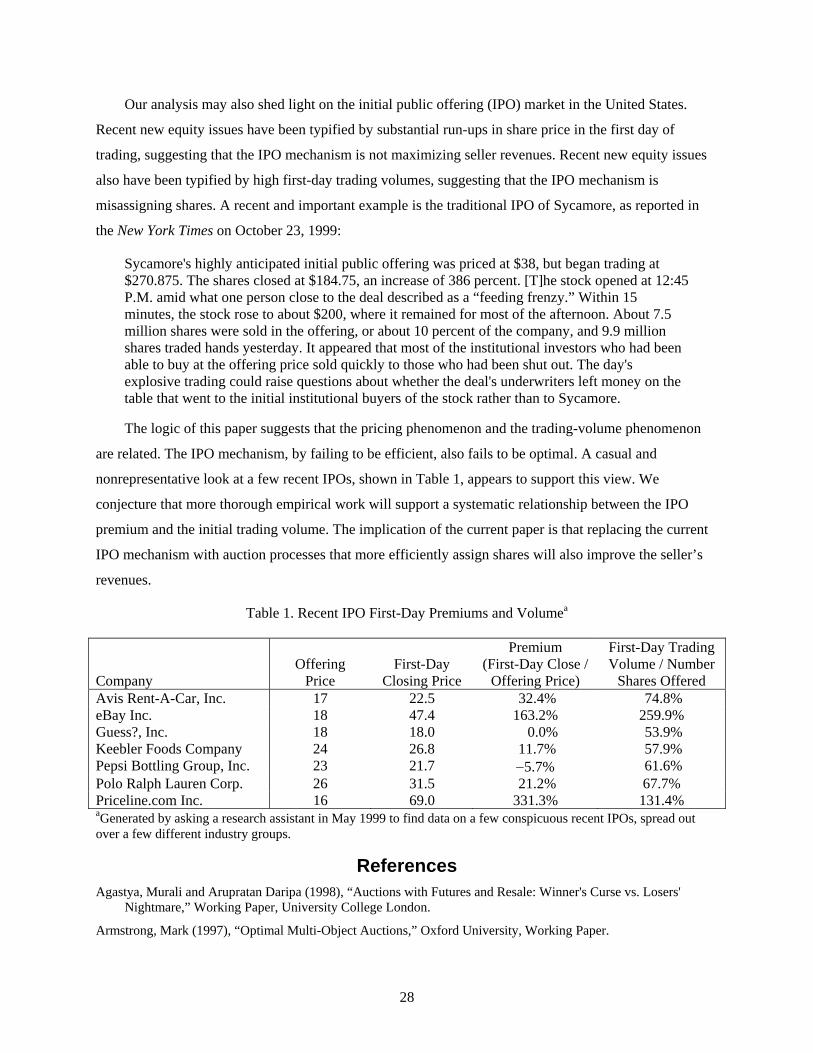
nonrepresentative look at a few recent IPOs, shown in Table 1, appears to support this view. We

conjecture that more thorough empirical work will support a systematic relationship between the IPO

premium and the initial trading volume. The implication of the current paper is that replacing the current

IPO mechanism with auction processes that more efficiently assign shares will also improve the seller’s

revenues.

Table 1. Recent IPO First-Day Premiums and Volumea

Company

Offering

Price

First-Day

Closing Price

Premium (First-Day Close /

Offering Price)

First-Day Trading Volume / Number

Shares Offered Avis Rent-A-Car, Inc. 17 22.5 32.4% 74.8% eBay Inc. 18 47.4 163.2% 259.9% Guess?, Inc. 18 18.0 0.0% 53.9% Keebler Foods Company 24 26.8 11.7% 57.9% Pepsi Bottling Group, Inc. 23 21.7 −5.7% 61.6% Polo Ralph Lauren Corp. 26 31.5 21.2% 67.7% Priceline.com Inc. 16 69.0 331.3% 131.4% aGenerated by asking a research assistant in May 1999 to find data on a few conspicuous recent IPOs, spread out over a few different industry groups.

References Agastya, Murali and Arupratan Daripa (1998), “Auctions with Futures and Resale: Winner's Curse vs. Losers'

Nightmare,” Working Paper, University College London.

Armstrong, Mark (1997), “Optimal Multi-Object Auctions,” Oxford University, Working Paper.

29

Ausubel, Lawrence M. (1997), “An Efficient Ascending-Bid Auction for Multiple Objects,” Working Paper, University of Maryland.

Ausubel, Lawrence M. and Peter Cramton (1998), “Demand Reduction and Inefficiency in Multi-Unit Auctions,” Working Paper, University of Maryland.

Ausubel, Lawrence M. and Peter Cramton (1999), “Notes on Vickrey Auctions with Reserve Pricing,” Working Paper, University of Maryland.

Ausubel, Lawrence M. and Raymond J. Deneckere (1989), “Reputation in Bargaining and Durable Goods Monopoly,” Econometrica, 57, 511-532.

Avery, Christopher and Terrance Hendershott (1998), “Bundling and Optimal Auctions of Multiple Goods,” Working Paper, Harvard University.

Bikhchandani, Sushil and Chi-fu Huang (1989), “Auctions with Resale Markets: An Exploratory Model of Treasury Bill Markets,” Review of Financial Studies, 2, 311-339.

Bulow, Jeremy and Paul Klemperer (1996), “Auctions vs. Negotiations,” American Economic Review, 86, 180-194.

Caillaud, Bernard and Jacques Robert (1998), “Implementing the Optimal Auction,” University of Montreal, Working Paper.

Coase, Ronald H. (1960), “The Problem of Social Cost,” Journal of Law and Economics, 3, 1-44.

Coase, Ronald H. (1972), “Durability and Monopoly,” Journal of Law and Economics, 15, 143-149.

Cramton, Peter, Robert Gibbons, and Paul Klemperer (1987), “Dissolving a Partnership Efficiently,” Econometrica, 55, 615-632.

Cremer, Jacques and Richard McLean (1988), “Full Extraction of the Surplus in Bayesian and Dominant Strategy Auctions,” Econometrica, 56, 1247-1258.

Cremer, Jacques and Michael H. Riordan (1985), “A Sequential Solution to the Public Goods Problem,” Econometrica, 53, 77-84.

Dasgupta, Partha and Eric Maskin (1997), “Notes on Efficient Auctions,” Working Paper, Harvard University.

Engelbrecht-Wiggans, Richard (1988), “Revenue Equivalence in Multi-object Auctions,” Economic Letters, 26, 15-19.

Haile, Philip A. (1996), “Auctions with Resale Markets: An Application to U.S. Forest Service Timber Sales,” Working Paper, University of Wisconsin.

Haile, Philip A. (1997), “Auctions with Private Uncertainty and Resale Opportunities,” Working Paper, University of Wisconsin.

Haile, Philip A. (1998), “Auctions with Resale,” Working Paper, University of Wisconsin.

Harstad, Ronald M. (1990), “Alternative Common-Value Auction Procedures: Revenue Comparisons with Free Entry,” Journal of Political Economy, 98, 421-429.

Harstad, Ronald M. (1993), “Auctions with Endogenous Bidder Participation,” Working Paper, Rutgers University.

Horstmann, J. Ignatius and Chantale LaCasse (1997), “Secret Reserve Prices in a Bidding Model with a Resale Option,” American Economic Review, 87, 663-684.

Krishna, Vijay and Motty Perry (1997), “Efficient Mechanism Design,” Working Paper, Penn State University.

Levin, Dan and James L. Smith (1994), “Equilibrium in Auctions with Entry,” American Economic Review, 84, 585-599.

Levin, Dan and James L. Smith (1995), “Auctions with Entry: An Experimental Investigation,” Working Paper, Ohio State University.

Levin, Dan and James L. Smith (1996), “Optimal Reservation Prices in Auctions,” Economic Journal, 106, forthcoming.

30

Maskin, Eric and John Riley (1989), “Optimal Multi-unit Auctions,” in Frank Hahn (ed) The Economics of Missing Markets, Information, and Games, Oxford: Oxford University Press, 312-35.

McAfee, R. Preston and John McMillan (1987), “Auctions with Entry,” Economic Letters, 23, 343-347.

McAfee, Preston R. and Philip Reny (1992), “Correlated Information and Mechanism Design,” Econometrica, 60, 395-422.

Myerson, Roger B. (1981), “Optimal Auction Design,” Mathematics of Operations Research, 6, 58-73.

Myerson, Roger B. and Mark A. Satterthwaite (1983), “Efficient Mechanisms for Bilateral Trading,” Journal of Economic Theory, 28, 265-281.

Vickrey, William (1961), “Counterspeculation, Auctions, and Competitive Sealed Tenders,” Journal of Finance, 16, 8-37.

Viswanathan, S. and James J.D. Wang (1996), “Auctions with When-Issued Trading: A Model of the U.S. Treasury Markets,” Working Paper, Duke University.