The Option KeyboardCombining Skills in Reinforcement Learning

André Barreto, Diana Borsa, Shaobo Hou, Gheorghe Comanici, Eser Aygün,Philippe Hamel, Daniel Toyama, Jonathan Hunt, Shibl Mourad, David Silver, Doina Precup

{andrebarreto,borsa,shaobohou,gcomanici,eser}@google.com

{hamelphi,kenjitoyama,jjhunt,shibl,davidsilver,doinap}@google.com

DeepMind

Abstract

The ability to combine known skills to create new ones may be crucial in thesolution of complex reinforcement learning problems that unfold over extendedperiods. We argue that a robust way of combining skills is to define and manipulatethem in the space of pseudo-rewards (or “cumulants”). Based on this premise, wepropose a framework for combining skills using the formalism of options. We showthat every deterministic option can be unambiguously represented as a cumulantdefined in an extended domain. Building on this insight and on previous resultson transfer learning, we show how to approximate options whose cumulants arelinear combinations of the cumulants of known options. This means that, once wehave learned options associated with a set of cumulants, we can instantaneouslysynthesise options induced by any linear combination of them, without any learninginvolved. We describe how this framework provides a hierarchical interface to theenvironment whose abstract actions correspond to combinations of basic skills.We demonstrate the practical benefits of our approach in a resource managementproblem and a navigation task involving a quadrupedal simulated robot.

1 Introduction

In reinforcement learning (RL) an agent takes actions in an environment in order to maximise theamount of reward received in the long run [25]. This textbook definition of RL treats actions asatomic decisions made by the agent at every time step. Recently, Sutton [23] proposed a new viewon action selection. In order to illustrate the potential benefits of his proposal Sutton resorts to thefollowing analogy. Imagine that the interface between agent and environment is a piano keyboard,with each key corresponding to a possible action. Conventionally the agent plays one key at a timeand each note lasts exactly one unit of time. If we expect our agents to do something akin to playingmusic, we must generalise this interface in two ways. First, we ought to allow notes to be arbitrarilylong—that is, we must replace actions with skills. Second, we should be able to also play chords.

The argument in favour of temporally-extended courses of actions has repeatedly been made in theliterature: in fact, the notion that agents should be able to reason at multiple temporal scales is one ofthe pillars of hierarchical RL [7, 18, 26, 8, 17]. The insight that the agent should have the ability tocombine the resulting skills is a far less explored idea. This is the focus of the current work.

The possibility of combining skills replaces a monolithic action set with a combinatorial counterpart:by learning a small set of basic skills (“keys”) the agent should be able to perform a potentially verylarge number of combined skills (“chords”). For example, an agent that can both walk and grasp anobject should be able to walk while grasping an object without having to learn a new skill. According

33rd Conference on Neural Information Processing Systems (NeurIPS 2019), Vancouver, Canada.

to Sutton [23], this combinatorial action selection process “could be the key to generating behaviourwith a good mix of preplanned coherence and sensitivity to the current situation.”

But how exactly should one combine skills? One possibility is to combine them in the space ofpolicies: for example, if we look at policies as distribution over actions, a combination of skills canbe defined as a mixture of the corresponding distributions. One can also combine parametric policiesby manipulating the corresponding parameters. Although these are feasible solutions, they fail tocapture possible intentions behind the skills. Suppose the agent is able to perform two skills that canbe associated with the same objective—distinct ways of grasping an object, say. It is not difficultto see how combinations of the corresponding behaviours can completely fail to accomplish thecommon goal. We argue that a more robust way of combining skills is to do so directly in the goalspace, using pseudo-rewards or cumulants [25]. If we associate each skill with a cumulant, we cancombine the former by manipulating the latter. This allows us to go beyond the direct prescription ofbehaviours, working instead in the space of intentions.

Combining skills in the space of cumulants poses two challenges. First, we must establish a well-defined mapping between cumulants and skills. Second, once a combined cumulant is defined, wemust be able to perform the associated skill without having to go through the slow process of learningit. We propose to tackle the former by adopting options as our formalism to define skills [26]. Weshow that there is a large subset of the space of options, composed of deterministic options, in whichevery element can be unambiguously represented as a cumulant defined in an extended domain.Building on this insight, we extend Barreto et al.’s [3, 4] previous results on transfer learning toshow how to approximate options whose cumulants are linear combinations of the cumulants ofknown options. This means that, once the agent has learned options associated with a collectionof cumulants, it can instantaneously synthesise options induced by any linear combination of them,without any learning involved. Thus, by learning a small set of options, the agent instantaneouslyhas at its disposal a potentially enormous number of combined options. Since we are combiningcumulants, and not policies, the resulting options will be truly novel, meaning that they cannot, ingeneral, be directly implemented as a simple alternation of their constituents.

We describe how our framework provides a flexible interface with the environment whose abstractactions correspond to combinations of basic skills. As a reference to the motivating analogy describedabove, we call this interface the option keyboard. We discuss the merits of the option keyboard at theconceptual level and demonstrate its practical benefits in two experiments: a resource managementproblem and a realistic navigation task involving a quadrupedal robot simulated in MuJoCo [30, 21].

2 Background

As usual, we assume the interaction between agent and environment can be modelled as a Markovdecision process (MDP) [19]. An MDP is a tupleM ≡ (S,A, p, r, γ), where S andA are the state andaction spaces, p(·|s, a) gives the next-state distribution upon taking action a in s, r : S ×A×S 7→ Rspecifies the reward associated with the transition s a−→ s′, and γ ∈ [0, 1) is the discount factor.

The objective of the agent is to find a policy π : S 7→ A that maximises the expected returnGt ≡

∑∞i=0 γ

iRt+i, where Rt = r(St, At, St+1). A principled way to address this problem is touse methods derived from dynamic programming, which usually compute the action-value functionof a policy π as: Qπ(s, a) ≡ Eπ [Gt|St = s,At = a] , where Eπ[·] denotes expectation over thetransitions induced by π [19]. The computation of Qπ(s, a) is called policy evaluation. Once π hasbeen evaluated, we can compute a greedy policy

π′(s) ∈ argmaxaQπ(s, a) for all s ∈ S. (1)

It can be shown that Qπ′(s, a) ≥ Qπ(s, a) for all (s, a) ∈ S ×A, and hence the computation of π′ is

referred to as policy improvement. The alternation between policy evaluation and policy improvementis at the core of many RL algorithms, which usually carry out these steps approximately. Here we willuse a tilde over a symbol to indicate that the associated quantity is an approximation (e.g., Qπ ≈ Qπ).

2.1 Generalising policy evaluation and policy improvement

Following Sutton and Barto [25], we call any signal defined as c : S × A × S 7→ R a cumulant.Analogously to the conventional value function Qπ , we define Qπc as the expected discounted sum of

2

cumulant c under policy π [27]. Given a policy π and a set of cumulants C, we call the evaluation ofπ under all c ∈ C generalised policy evaluation (GPE) [2]. Barreto et al. [3, 4] propose an efficientform of GPE based on successor features: they show that, given cumulants c1, c2, ..., cd, for anyc =

∑i wici, with w ∈ Rd,

Qπc (s, a) ≡ Eπ[ ∞∑k=0

γkd∑i=1

wiCi,t+k|St = s,At = a

]=

d∑i=1

wiQπci(s, a), (2)

whereCi,t ≡ ci(St, At, Rt). Thus, once we have computedQπc1 , Qπc1 , ..., Q

πcd

, we can instantaneouslyevaluate π under any cumulant in the set C ≡ {c =

∑i wici |w ∈ Rd}.

Policy improvement can also be generalised. In Barreto et al.’s [3] generalised policy improvement(GPI) the improved policy is computed based on a set of value functions. Let Qπ1

c , Qπ2c , ...Q

πnc be

the action-value functions of n policies πi under cumulant c, and let Qmaxc (s, a) = maxiQ

πic (s, a)

for all (s, a) ∈ S ×A. If we define

π(s) ∈ argmaxaQmaxc (s, a) for all s ∈ S, (3)

then Qπc (s, a) ≥ Qmaxc (s, a) for all (s, a) ∈ S ×A. This is a strict generalisation of standard policy

improvement (1). The guarantee extends to the case in which GPI uses approximations Qπic [3].

2.2 Temporal abstraction via options

As discussed in the introduction, one way to get temporal abstraction is through the concept ofoptions [26]. Options are temporally-extended courses of actions. In their more general formulation,options can depend on the entire history between the time t when they were initiated and the currenttime step t + k, ht:t+k ≡ statst+1...at+k−1st+k. Let H be the space of all possible histories; asemi-Markov option is a tuple o ≡ (Io, πo, βo) where Io ⊂ S is the set of states where the option canbe initiated, πo : H 7→ A is a policy over histories, and βo : H 7→ [0, 1] gives the probability that theoption terminates after history h has been observed [26]. It is worth emphasising that semi-Markovoptions depend on the history since their initiation, but not before.

3 Combining optionsIn the previous section we discussed how several key concepts in RL can be generalised: rewardswith cumulants, policy evaluation with GPE, policy improvement with GPI, and actions with options.In this section we discuss how these concepts can be used to combine skills.

3.1 The relation between options and cumulants

We start by showing that there is a subset of the space of options in which every option can beunequivocally represented as a cumulant defined in an extended domain.

First we look at the relation between policies and cumulants. Given an MDP (S,A, p, ·, γ), we saythat a cumulant cπ : S × A × S 7→ R induces a policy π : S 7→ A if π is optimal for the MDP(S,A, p, cπ, γ). We can always define a cumulant cπ that induces a given policy π. For instance, ifwe make

cπ(s, a, ·) ={

0 if a = π(s);z otherwise, (4)

where z < 0, it is clear that π is the only policy that achieves the maximum possible valueQπ(s, a) =Q∗(s, a) = 0 on all (s, a) ∈ S × A. In general, the relation between policies and cumulants is amany-to-many mapping. First, there is more than one cumulant that induces the same policy: forexample, any z < 0 in (4) will clearly lead to the same policy π. There is thus an infinite set ofcumulants Cπ associated with π. Conversely, although this is not the case in (4), the same cumulantcan give rise to multiple policies if more than one action achieves the maximum in (1).

Given the above, we can use any cumulant cπ ∈ Cπ to refer to policy π. In order to extend thispossibility to options o = (Io, πo, βo) we need two things. First, we must define cumulants in thespace of historiesH. This will allow us to induce semi-Markov policies πo : H 7→ A in a way that isanalogous to (4). Second, we need cumulants that also induce the initiation set Io and the terminationfunction βo. We propose to accomplish this by augmenting the action space.

3

Let τ be a termination action that terminates option o much like the termination function βo. We canthink of τ as a fictitious action and model it by defining an augmented action space A+ ≡ A ∪ {τ}.When the agent is executing an option o, selecting action τ immediately terminates it. We nowshow that if we extend the definition of cumulants to also include τ we can have the resultingcumulant induce not only the option’s policy but also its initiation set and termination function. Lete : H×A+ × S 7→ R be an extended cumulant. Since e is defined over the augmented action space,for each h ∈ H we now have a termination bonus e(h, τ, s) = e(h, τ) that determines the value ofinterrupting option o after having observed h. The extended cumulant e induces an augmented policyωe : H 7→ A+ in the same sense that a standard cumulant induces a policy (that is, ωe is an optimalpolicy for the derived MDP whose state space isH and the action space is A+; see Appendix A fordetails). We argue that ωe is equivalent to an option oe ≡ (Ie, πe, βe) whose components are definedas follows. The policy πe : H 7→ A coincides with ωe whenever the latter selects an action in A. Thetermination function is given by

βe(h) =

{1 if e(h, τ) > maxa 6=τ Qωe

e (h, a),0 otherwise. (5)

In words, the agent will terminate after h if the instantaneous termination bonus e(h, τ) is larger thanthe maximum expected discounted sum of cumulant e under policy ωe. Note that when h is a singlestate s, no concrete action has been executed by the option yet, hence it terminates with τ immediatelyafter its initiation. This is precisely the definition of the initialisation set Ie ≡ {s |βe(s) = 0}.Termination functions like (5) are always deterministic. This means that extended cumulants e canonly represent options oe in which βe is a mappingH 7→ {0, 1}. In fact, it is possible to show thatall options of this type, which we will call deterministic options, are representable as an extendedcumulant e, as formalised in the following proposition (proof in Appendix A):Proposition 1. Every extended cumulant induces at least one deterministic option, and every deter-ministic option can be unambiguously induced by an infinite number of extended cumulants.

3.2 Synthesising options using GPE and GPI

In the previous section we looked at the relation between extended cumulants and deterministicoptions; we now build on this connection to use GPE and GPI to combine options.

Let E ≡ {e1, e2, ..., ed} be a set of extended cumulants. We know that ei : H × A+ × S 7→ R isassociated with deterministic option oei ≡ ωei . As with any other cumulant, the extended cumulantsei can be linearly combined; it then follows that, for any w ∈ Rd, e =

∑i wiei defines a new

deterministic option oe ≡ ωe. Interestingly, the termination function of oe has the form (5) withtermination bonuses defined as e(h, τ) =

∑i wiei(h, τ). This means that the combined option oe

“inherits” its termination function from its constituents oei . Since any w ∈ Rd defines an option oe,the set E can give rise to a very large number of combined options.

The problem is of course that for each w ∈ Rd we have to actually compute the resulting option ωe.This is where GPE and GPI come to the rescue. Suppose we have the values of options ωei under allthe cumulants e1, e2, ..., ed. With this information, and analogously to (2), we can use the fast formof GPE provided by successor features to compute the value of ωej with respect to e:

Qωeje (h, a) =

∑i

wiQωejei (h, a). (6)

Now that we have all the options ωej evaluated under e, we can merge them to generate a new optionthat does at least as well as, and in general better than, all of them. This is done by applying GPI overthe value functions Q

ωeje :

ωe(h) ∈ argmaxa∈A+ maxj Qωeje (h, a). (7)

From previous theoretical results we know that maxj Qωeje (h, a) ≤ Qωe

e (h, a) ≤ Qωee (h, a) for all

(h, a) ∈ H ×A+ [3]. In words, this means that, even though the GPI option ωe is not necessarilyoptimal, following it will in general result in a higher return in terms of cumulant e than if the agentwere to execute any of the known options ωej . Thus, we can use ωe as an approximation to ωe thatrequires no additional learning. It is worth mentioning that the action selected by the combinedoption in (7), ωe(h), can be different from ωei(h) for all i—that is, the resulting policy cannot, in

4

general, be implemented as an alternation of its constituents. This highlights the fact that combiningcumulants is not the same as defining a higher-level policy over the associated options.

In summary, given a set of cumulants E , we can combine them by picking weights w and computingthe resulting cumulant e =

∑i wiei. This can be interpreted as determining how desirable or

undesirable each cumulant is. Going back to the example in the introduction, suppose that e1 isassociated with walking and e2 is associated with grasping an object. Then, cumulant e1 + e2 willreinforce both behaviours, and will be particularly rewarding when they are executed together. Incontrast, cumulant e1 − e2 will induce an option that avoids grasping objects, favouring the walkingbehaviour in isolation and even possibly inhibiting it. Since the resulting option aims at maximising acombination of the cumulants ei, it can itself be seen as a combination of the options oei .

4 Learning with combined options

player environmentw a

r, sr′, s′, γ′

agent

OK

temporal abstraction

Figure 1: OK mediates the interaction between playerand environment. The exchange of information betweenOK and the environment happens at every time step.The interaction between player and OK only happens“inside” the agent when the termination action τ is se-lected by GPE and GPI (see Algorithms 1 and 2).

Given a set of extended cumulants E , inorder to be able to combine the asso-ciated options using GPE and GPI oneonly needs the value functions QE ≡{Qωei

ej | ∀(i, j) ∈ {1, 2, ..., d}2}. The setQE can be constructed using standard RLmethods; for an illustration of how to do itwith Q-learning see Algorithm 3 in App. B.

As discussed, once QE has been computedwe can use GPE and GPI to synthesise op-tions on the fly. In this case the newly-generated options are fully determined bythe vector of weights w ∈ Rd. Concep-tually, we can think of this process as aninterface between an RL algorithm and the environment: the algorithm selects a vector w, hands itover to GPE and GPI, and “waits” until the action returned by (7) is the termination action τ . Once τhas been selected, the algorithm picks a new w, and so on. The RL method is thus interacting withthe environment at a higher level of abstraction in which actions are combined skills defined by thevectors of weights w. Returning to the analogy with a piano keyboard described in the introduction,we can think of each option ωei as a “key” that can be activated by an instantiation of w whose onlynon-zero entry is wi > 0. Combined options associated with more general instantiations of w wouldcorrespond to “chords”. We will thus call the layer of temporal abstraction between algorithm andenvironment the option keyboard (OK). We will also generically refer to the RL method interactingwith OK as the “player”. Figure 1 shows how an RL agent can be broken into a player and an OK.

Algorithm 1 shows a generic implementation of OK. Given a set of value functions QE and a vectorof weights w, OK will execute the actions selected by GPE and GPI until the termination action ispicked or a terminal state is reached. During this process OK keeps track of the discounted rewardaccumulated in the interaction with the environment (line 6), which will be returned to the playerwhen the interaction terminates (line 10). As the options ωei may depend on the entire trajectorysince their initiation, OK uses an update function u(h, a, s′) that retains the parts of the history thatare actually relevant for decision making (line 8). For example, if OK is based on Markov optionsonly, one can simply use the update function u(h, a, s′) = s′.

The set QE defines a specific instantiation of OK; once an OK is in place any conventional RLmethod can interact with it as if it were the environment. As an illustration, Algorithm 2 showshow a keyboard player that uses a finite set of combined options W ≡ {w1,w2, ...,wn} can beimplemented using standard Q-learning by simply replacing the environment with OK. It is worthpointing out that if we substitute any other set of weight vectorsW ′ forW we can still use the sameOK, without the need to relearn the value functions in QE . We can even use sets of abstract actionsW that are infinite—as long as the OK player can deal with continuous action spaces [33, 24, 22].

Although the clear separation between OK and its player is instructive, in practice the boundarybetween the two may be more blurry. For example, if the player is allowed to intervene in all interac-tions between OK and environment, one can implement useful strategies like option interruption [26].Finally, note that although we have been treating the construction of OK (Algorithm 3) and its use

5

(Algorithms 1 and 2) as events that do not overlap in time, nothing keeps us from carrying out thetwo procedures in parallel, like in similar methods in the literature [1, 32].

Algorithm 1 Option Keyboard (OK)

Require:

s ∈ S current statew ∈ Rd vector of weightsQE value functionsγ ∈ [0, 1) discount rate

1: h← s; r′ ← 0; γ′ ← 12: repeat3: a← argmaxa′ maxi[

∑j wjQ

ωeiej (h, a′)]

4: if a 6= τ then5: execute action a and observe r and s′6: r′ ← r′ + γ′r7: if s′ is terminal γ′ ← 0 else γ′ ← γ′γ8: h← u(h, a, s′)9: until a = τ or s′ is terminal

10: return s′, r′, γ′

Algorithm 2 Q-learning keyboard player

Require:

OK option keyboardW combined optionsQE value functionsα, ε, γ ∈ R hyper-parameters

1: create Q(s,w) parametrised by θQ2: select initial state s ∈ S3: repeat forever4: if Bernoulli(ε)=1 then w ← Uniform(W)5: else w ← argmaxw′∈WQ(s,w′)6: (s′, r′, γ′)← OK(s, w, QE , γ)7: δ ← r′ + γ′maxw′ Q(s′,w′)− Q(s,w)

8: θQ ← θQ + αδ∇θQQ(s,w) // update Q

9: if s′ is terminal then select initial s ∈ S10: else s← s′

5 Experiments

We now present our experimental results illustrating the benefits of OK in practice. Additional details,along with further results and analysis, can be found in Appendix C.

5.1 Foraging worldThe goal in the foraging world is to manage a set of resources by navigating in a grid world andpicking up items containing the resources in different proportions. For illustrative purposes we willconsider that the resources are nutrients and the items are food. The agent’s challenge is to stayhealthy by keeping its nutrients within certain bounds. The agent navigates in the grid world usingthe four usual actions: up, down, left, and right. Upon collecting a food item the agent’s nutrients areincreased according to the type of food ingested. Importantly, the quantity of each nutrient decreasesby a fixed amount at every step, so the desirability of different types of food changes even if no food isconsumed. Observations are images representing the configuration of the grid plus a vector indicatinghow much of each nutrient the agent currently has (see Appendix C.1 for a technical description).

What makes the foraging world particularly challenging is the fact that the agent has to travel towardsthe items to pick them up, adding a spatial aspect to an already complex management problem. Thedual nature of the problem also makes it potentially amenable to be tackled with options, since wecan design skills that seek specific nutrients and then treat the problem as a management task inwhich actions are preferences over nutrients. However, the number of options needed can increaseexponentially fast. If at any given moment the agent wants, does not want, or does not care abouteach nutrient, we need 3m options to cover the entire space of preferences, where m is the number ofnutrients. This is a typical situation where being able to combine skills can be invaluable.

As an illustration, in our experiments we used m = 2 nutrients and 3 types of food. We defineda cumulant ei ∈ E associated with each nutrient as follows: ei(h, a, s) = 0 until a food item isconsumed, when it becomes the increase in the associated nutrient. After a food item is consumed wehave that ei(h, a, s) = −1{a 6= τ}, where 1{·} is the indicator function—this forces the inducedoption to terminate, and also illustrates how the definition of cumulants over histories h can be useful(since single states would not be enough to determine whether the agent has consumed a food item).We used Algorithm 3 in Appendix B to compute the 4 value functions in QE . We then defined a8-dimensional abstract action space covering the space of preferences,W ≡ {−1, 0, 1}2 − {[0, 0]},and used it with the Q-learning player in Algorithm 2. We also consider Q-learning using only the 2options maximizing each nutrient and a “flat” Q-learning agent that does not use options at all.

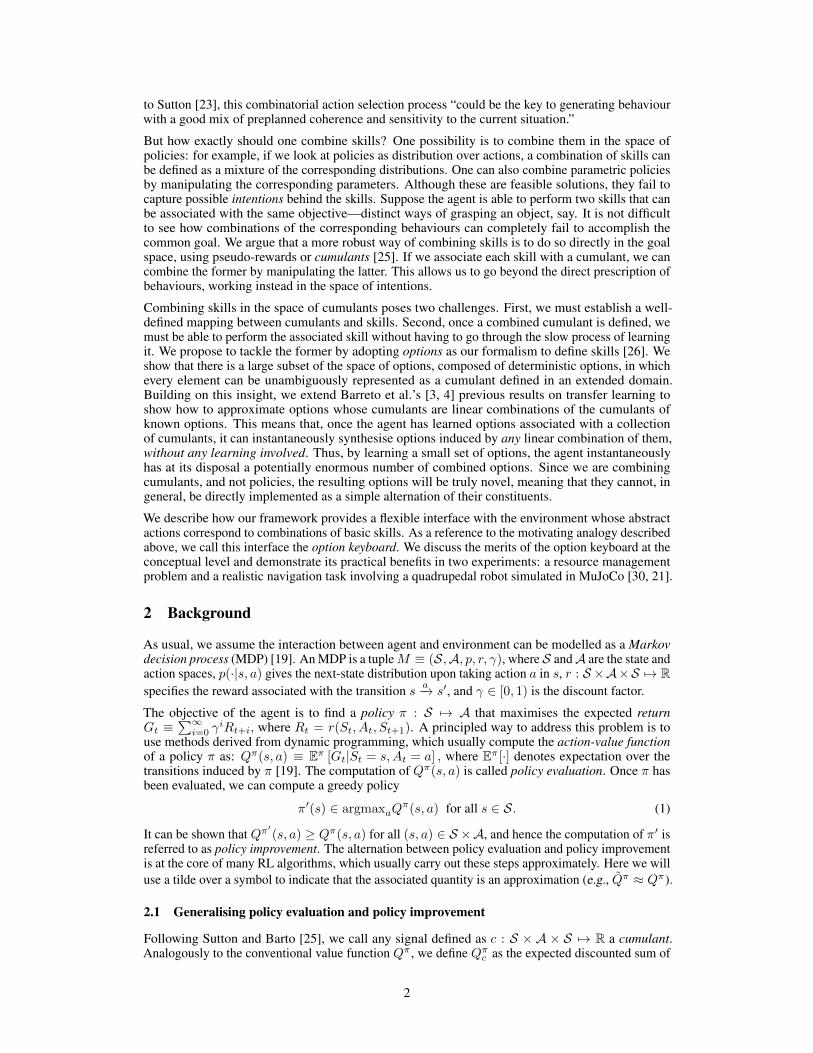
By modifying the target range of each nutrient we can create distinct scenarios with very differentdynamics. Figure 2 shows results in two such scenarios. Note how the relative performance of thetwo baselines changes dramatically from one scenario to the other, illustrating how the usefulnessof options is highly context-dependent. Importantly, as shown by the results of the OK player, the

6

0 200000 400000 600000 800000 1000000

steps

0

20

40

60

80

100

120

140

160

Avera

ge E

pis

ode R

etu

rn

Q-Learning Player

Q-Learning Simple Options

Q-Learning

0 200000 400000 600000 800000 1000000

steps

40

20

0

20

40

60

80

100

Avera

ge E

pis

ode R

etu

rn

Q-Learning Player

Q-Learning Simple Options

Q-Learning

Figure 2: Results on the foraging world. The two plots correspond to different configurations of theenvironment (see Appendix C.1). Shaded regions are one standard deviation over 10 runs.

ability to combine options in cumulant space makes it possible to synthesise useful behaviour from agiven set of options even when they are not useful in isolation.

5.2 Moving-target arenaAs the name suggests, in the moving-target arena the goal is to get to a target region whose locationchanges every time the agent reaches it. The arena is implemented as a square room with realisticdynamics defined in the MuJoCo physics engine [30]. The agent is a quadrupedal simulated robotwith 8 actuated degrees of freedom; actions are thus vectors in [−1, 1]8 indicating the torque applied toeach joint [21]. Observations are 29-dimensional vectors with spatial and proprioception information(Appendix C.2). The reward is always 0 except when the agent reaches the target, when it is 1.

We defined cumulants in order to encourage the agent’s displacement in certain directions. Let v(h)be the vector of (x, y) velocities of the agent after observing history h (the velocity is part of theobservation). Then, if we want the agent to travel at a certain direction w for k steps, we can define:

ew(h, a, ·) ={w>v(h) if length(h) ≤ k;−1{a 6= τ} otherwise. (8)

The induced option will terminate after k = 8 steps as a negative reward is incurred for all historiesof length greater than k and actions other than τ . It turns out that even if a larger number of directionsw is to be learned, we only need to compute two value functions for each cumulant ew. Since forall ew ∈ E we have that ew = w1ex + w2ey, where x = [1, 0] and y = [0, 1], we can use (2) todecompose the value function of any option ω as Qωew(h, a) = w1Q

ωex(h, a) + w2Q

ωey (h, a). Hence,

|QE | = 2|E|, resulting in a 2-dimensional spaceW in whichw ∈ R2 indicates the intended directionof locomotion. Thus, by learning a few options that move along specific directions, the agent ispotentially able to synthesise options that travel in any direction.

For our experiments, we defined cumulants ew corresponding to the directions 0o, 120o, and 240o.To compute the set of value functions QE we used Algorithm 3 with Q-learning replaced by thedeterministic policy gradient (DPG) algorithm [22]. We then used the resulting OK with both discreteand continuous abstract-action spacesW . For finiteW we adopted aQ-learning player (Algorithm 2);in this case the abstract actions wi correspond to n ∈ {4, 6, 8} directions evenly-spaced in the unitcircle. For continuousW we used a DPG player. We compare OK’s results with that of DPG applieddirectly in the original action space and also with Q-learning using only the three basic options.

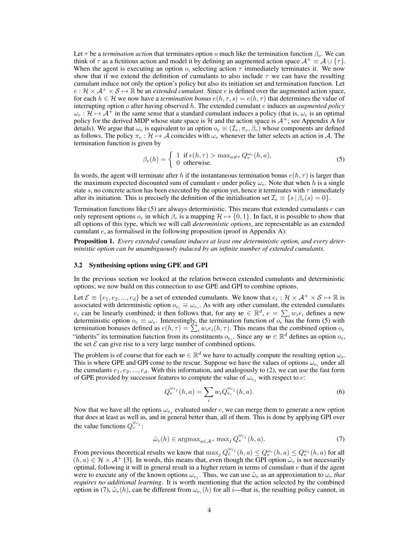
Figure 3 shows our results on the moving-target arena. As one can see by DPG’s results, solvingthe problem in the original action space is difficult because the occurrence of non-zero rewards maydepend on a long sequence of lucky actions. When we replace actions with options we see a clearspeed up in learning, even if we take into account the training of the options. If in addition we allowfor combined options, we observe a significant boost in performance, as shown by the OK players’results. Here we see the expected trend: as we increase |W| the OK player takes longer to learn butachieves better final performance, as larger numbers of directional options allow for finer control.

These results clearly illustrate the benefits of being able to combine skills, but how much is the agentactually using this ability? In Figure 3 we show a histogram indicating how often combined optionsare used by OK to implement directions w ∈ R2 across the state space (details in App. C.2). Asshown, for abstract actions w close to 0o, 120o and 240o the agent relies mostly on the 3 optionstrained to navigate along these directions, but as the intended direction of locomotion gets farther from

7

0 1 2 3 4 5

Steps 1e7

0

5

10

15

20

25

30

35

Avera

ge r

etu

rn p

er

epis

ode

OK training

DPG PlayerQ-Learning Player (8)Q-Learning Player (6)Q-Learning Player (4)Q-Learning + OptionsDPG

Figure 3: Left: Results on the moving-target arena. All players used the same keyboard, so theyshare the same OK training phase. Shaded regions are one standard deviation over 10 runs. Right:Histogram of options used by OK to implement directionsw. Black lines are the three basic options.

these reference points combined options become crucial. This shows how the ability to combine skillscan extend the range of behaviours available to an agent without the need for additional learning.1

Even if one accepts the premise of this paper that skills should be combined in the space of cumulants,it is natural to ask whether other strategies could be used instead of GPE and GPI. Although we arenot aware of any other algorithm that explicitly attempts to combine skills in the space of cumulants,there are methods that do so in the space of value functions [29, 6, 13, 16]. Haarnoja et al. [13]propose a way of combining skills based on entropy-regularised value functions. Given a set ofcumulants e1, e2, ..., ed, they propose to compute a skill associated with e =

∑i wiei as follows:

ωe(h) ∈ argmaxa∈A+

∑j wjQ

ωejej (h, a), where Q

ωejej (h, a) are entropy-regularised value functions

and wj ∈ [−1, 1]. We will refer to this method as additive value composition (AVC).

How well does AVC perform as compared to GPE and GPI? In order to answer this question wereran the previous experiments but now using ωe(h) as defined above instead of the option ωe(h)computed through (6) and (7). In order to adhere more closely to the assumptions underlying AVC,we also repeated the experiment using an entropy-regularised OK [14] (App. C.2). Figure 4 showsthe results. As indicated in the figure, GPE and GPI outperform AVC both with the standard and theentropy-regularised OK. A possible explanation for this is given in the accompanying polar scatterchart in Figure 4, which illustrates how much progress each method makes, over the state space, in alldirections w (App. C.2). The plot suggests that, in this domain, the directional options implementedthrough GPI and GPE are more effective in navigating along the desired directions (also see [16]).

6 Related workPrevious work has used GPI and successor features, the linear form of GPE considered here, in thecontext of transfer [3, 4, 5]. A crucial assumption underlying these works is that the reward canbe well approximated as r(s, a, s′) ≈

∑i wici(s, a, s

′). By solving a regression problem, the agentfinds a w ∈ Rd that leads to a good approximation of r(s, a, s′) and uses it to apply GPE and GPI(equations (2) and (3), respectively). In terms of the current work, this is equivalent to having akeyboard player that is only allowed to play one endless “chord”. Through the introduction of atermination action, in this work we replace policies with options that may eventually halt. Sincepolicies are options that never terminate, the previous framework is a special case of OK. Unlike inthe previous framework, with OK we can also chain a sequence of options, resulting in more flexiblebehaviour. Importantly, this allows us to completely remove the linearity assumption on the rewards.

We now turn our attention to previous attempts to combine skills with no additional learning. Asdiscussed, one way to do so is to work directly in the space of policies. Many policy-based methodsfirst learn a parametric representation of a lower-level policy, π(·| s;θ), and then use θ ∈ Rd as theactions for a higher-level policy µ : S 7→ Rd [15, 10, 12]. One of the central arguments of this paper

1A video of the quadrupedal simulated robot being controlled by the DPG player can be found on thefollowing link: https://youtu.be/39Ye8cMyelQ.

8

0 1 2 3 4 5

Steps 1e7

0

5

10

15

20

25

30

35

Avera

ge r

etu

rn p

er

epis

ode

OK training

GPE and GPI + OKGPE and GPI + ENT-OKAVC + OKAVC + ENT-OKDPG

Figure 4: Left: Comparison of GPE and GPI with AVC on the moving-target arena. Results wereobtained by a DPG player using a standard OK and an entropy-regularised counterpart (ENT-OK).We trained several ENT-OK with different regularisation parameters and picked the one leading to thebest AVC performance. The same player and keyboards were used for both methods. Shaded regionsare one standard deviation over 10 runs. Right: Polar scatter chart showing the average distancetravelled by the agent along directions w when combining options using the two competing methods.

is that combining skills in the space of cumulants may be advantageous because it corresponds tomanipulating the goals underlying the skills. This can be seen if we think of w ∈ Rd as a way ofencoding skills and compare its effect on behaviour with that of θ: although the option induced byw1 +w2 through (6) and (7) will seek a combination of both its constituent’s goals, the same cannotbe said about a skill analogously defined as π(·| s; θ1 + θ2). More generally, though, one shouldexpect both policy- and cumulant-based approaches to have advantages and disadvantages.

Interestingly, most of the previous attempts to combine skills in the space of value functions are basedon entropy-regularised RL, like the already discussed AVC [34, 9, 11, 13]. Hunt et al. [16] propose away of combining skills which can in principle lead to optimal performance if one knows in advancethe weights of the intended combinations. They also extend GPE and GPI to entropy-regularisedRL. Todorov [28] focuses on entropy-regularised RL on linearly solvable MDPs. Todorov [29] andda Silva et al. [6] have shown how, in this scenario, one can compute optimal skills correspondingto linear combinations of other optimal skills—a property later explored by Saxe et al. [20] topropose a hierarchical approach. Along similar lines, Van Niekerk et al. [31] have shown howoptimal value function composition can be obtained in entropy-regularised shortest-path problemswith deterministic dynamics, with the non-regularised setup as a limiting case.

7 ConclusionThe ability to combine skills makes it possible for an RL agent to learn a small set of skills andthen use them to generate a potentially very large number of distinct behaviours. A robust way ofcombining skills is to do so in the space of cumulants, but in order to accomplish this one needsto solve two problems: (1) establish a well-defined mapping between cumulants and skills and (2)define a mechanism to implement the combined skills without having to learn them.

The two main technical contributions of this paper are solutions for these challenging problems. First,we have shown that every deterministic option can be induced by a cumulant defined in an extendeddomain. This novel theoretical result provides a way of thinking about options whose interest maygo beyond the current work. Second, we have described how to use GPE and GPI to synthesisecombined options on-the-fly, with no learning involved. To the best of our knowledge, this is the onlymethod to do so in general MDPs with performance guarantees for the combined options.

We used the above formalism to introduce OK, an interface to an RL problem in which actionscorrespond to combined skills. Since OK is compatible with essentially any RL method, it can bereadily used to endow our agents with the ability to combine skills. In describing the analogy with akeyboard that inspired our work, Sutton [23] calls for the need of “something larger than actions, butmore combinatorial than the conventional notion of options.” We believe OK provides exactly that.

9

Acknowledgements

We thank Joseph Modayil for first bringing the subgoal keyboard idea to our attention, and alsofor the subsequent discussions on the subject. We are also grateful to Richard Sutton, Tom Schaul,Daniel Mankowitz, Steven Hansen, and Tuomas Haarnoja for the invaluable conversations that helpedus develop our ideas and improve the paper. Finally, we thank the anonymous reviewers for theircomments and suggestions.

References[1] P. Bacon, J. Harb, and D. Precup. The option-critic architecture. In Proceedings of the AAAI

Conference on Artificial Intelligence (AAAI), 2017.

[2] A. Barreto, S. Hou, D. Borsa, D. Silver, and D. Precup. Fast reinforcement learning withgeneralized policy updates. Manuscript in preparation.

[3] A. Barreto, W. Dabney, R. Munos, J. Hunt, T. Schaul, H. van Hasselt, and D. Silver. Successorfeatures for transfer in reinforcement learning. In Advances in Neural Information ProcessingSystems (NIPS), 2017.

[4] A. Barreto, D. Borsa, J. Quan, T. Schaul, D. Silver, M. Hessel, D. Mankowitz, A. Zidek, andR. Munos. Transfer in deep reinforcement learning using successor features and generalisedpolicy improvement. In Proceedings of the International Conference on Machine Learning(ICML), 2018.

[5] D. Borsa, A. Barreto, J. Quan, D. J. Mankowitz, H. van Hasselt, R. Munos, D. Silver, andT. Schaul. Universal successor features approximators. In International Conference on LearningRepresentations (ICLR), 2019.

[6] M. da Silva, F. Durand, and J. Popovic. Linear Bellman combination for control of characteranimation. ACM Transactions on Graphics, 28(3):82:1–82:10, 2009.

[7] P. Dayan and G. E. Hinton. Feudal reinforcement learning. In Advances in Neural InformationProcessing Systems (NIPS), 1993.

[8] T. G. Dietterich. Hierarchical reinforcement learning with the MAXQ value function decompo-sition. Journal of Artificial Intelligence Research, 13:227–303, 2000.

[9] R. Fox, A. Pakman, and N. Tishby. Taming the noise in reinforcement learning via soft updates.In Proceedings of the Conference on Uncertainty in Artificial Intelligence (UAI), 2016.

[10] K. Frans, J. Ho, X. Chen, P. Abbeel, and J. Schulman. Meta learning shared hierarchies. InInternational Conference on Learning Representations (ICLR), 2018.

[11] T. Haarnoja, H. Tang, P. Abbeel, and S. Levine. Reinforcement learning with deep energy-basedpolicies. In Proceedings of the International Conference on Machine Learning (ICML), 2017.

[12] T. Haarnoja, K. Hartikainen, P. Abbeel, and S. Levine. Latent space policies for hierarchicalreinforcement learning. In Proceedings of the International Conference on Machine Learning(ICML), 2018.

[13] T. Haarnoja, V. Pong, A. Zhou, M. Dalal, P. Abbeel, and S. Levine. Composable deep reinforce-ment learning for robotic manipulation. In IEEE International Conference on Robotics andAutomation (ICRA), 2018.

[14] T. Haarnoja, A. Zhou, P. Abbeel, and S. Levine. Soft actor-critic: Off-policy maximumentropy deep reinforcement learning with a stochastic actor. In Proceedings of the InternationalConference on Machine Learning (ICML), 2018.

[15] N. Heess, G. Wayne, Y. Tassa, T. P. Lillicrap, M. A. Riedmiller, and D. Silver. Learningand transfer of modulated locomotor controllers. CoRR, abs/1610.05182, 2016. URL http://arxiv.org/abs/1610.05182.

10

[16] J. J. Hunt, A. Barreto, T. P. Lillicrap, and N. Heess. Entropic policy composition with generalizedpolicy improvement and divergence correction. In Proceedings of the International Conferenceon Machine Learning (ICML), 2019.

[17] L. P. Kaelbling. Hierarchical learning in stochastic domains: Preliminary results. In Proceedingsof the International Conference on Machine Learning (ICML), 2014.

[18] R. Parr and S. Russell. Reinforcement learning with hierarchies of machines. In Proceedings ofthe Conference on Advances in Neural Information Processing Systems (NIPS), 1997.

[19] M. L. Puterman. Markov Decision Processes—Discrete Stochastic Dynamic Programming.John Wiley & Sons, Inc., 1994.

[20] A. M. Saxe, A. C. Earle, and B. Rosman. Hierarchy through composition with multitaskLMDPS. In Proceedings of the International Conference on Machine Learning (ICML), 2017.

[21] J. Schulman, P. Moritz, S. Levine, M. Jordan, and P. Abbeel. High-dimensional continuouscontrol using generalized advantage estimation. In Proceedings of the International Conferenceon Learning Representations (ICLR), 2016.

[22] D. Silver, G. Lever, N. Heess, T. Degris, D. Wierstra, and M. Riedmiller. Deterministic policygradient algorithms. In Proceedings of the International Conference on Machine Learning(ICML), 2014.

[23] R. Sutton. Toward a new view of action selection: The subgoal keyboard. Slides presentedat the Barbados Workshop on Reinforcement Learning, 2016. URL http://barbados2016.rl-community.org/RichSutton2016.pdf?attredirects=0&d=1.

[24] R. Sutton, D. McAllester, S. Singh, and Y. Mansour. Policy gradient methods for reinforcementlearning with function approximation. In Advances in Neural Information Processing Systems(NIPS), 2000.

[25] R. S. Sutton and A. G. Barto. Reinforcement Learning: An Introduction. MIT Press, 2018.

[26] R. S. Sutton, D. Precup, and S. Singh. Between MDPs and semi-MDPs: a framework fortemporal abstraction in reinforcement learning. Artificial Intelligence, 112:181–211, 1999.

[27] R. S. Sutton, J. Modayil, M. Delp, T. Degris, P. M. Pilarski, A. White, and D. Precup. Horde:A scalable real-time architecture for learning knowledge from unsupervised sensorimotorinteraction. In International Conference on Autonomous Agents and Multiagent Systems(AMAS), 2011.

[28] E. Todorov. Linearly-solvable Markov decision problems. In Advances in Neural InformationProcessing Systems (NIPS), 2007.

[29] E. Todorov. Compositionality of optimal control laws. In Advances in Neural InformationProcessing Systems (NIPS), 2009.

[30] E. Todorov, T. Erez, and Y. Tassa. MuJoCo: A physics engine for model-based control. InIntelligent Robots and Systems (IROS), 2012.

[31] B. Van Niekerk, S. James, A. Earle, and B. Rosman. Composing value functions in reinforcementlearning. In Proceedings of the International Conference on Machine Learning (ICML), 2019.

[32] A. S. Vezhnevets, S. Osindero, T. Schaul, N. Heess, M. Jaderberg, D. Silver, and K. Kavukcuoglu.FeUdal networks for hierarchical reinforcement learning. In Proceedings of the InternationalConference on Machine Learning (ICML), pages 3540–3549, 2017.

[33] R. J. Williams. Simple statistical gradient-following algorithms for connectionist reinforcementlearning. Machine Learning, 8:229–256, 1992.

[34] B. D. Ziebart. Modeling Purposeful Adaptive Behavior with the Principle of Maximum CausalEntropy. PhD thesis, Carnegie Mellon University, 2010.

11

The Option KeyboardCombining Skills in Reinforcement Learning

Supplementary Material

André Barreto, Diana Borsa, Shaobo Hou, Gheorghe Comanici, Eser Aygün,Philippe Hamel, Daniel Toyama, Jonathan Hunt, Shibl Mourad, David Silver, Doina Precup

{andrebarreto,borsa,shaobohou,gcomanici,eser}@google.com

{hamelphi,kenjitoyama,jjhunt,shibl,davidsilver,doinap}@google.com

DeepMind

Abstract

In this supplement we give details of the theory and experiments that had to be leftout of the main paper due to space constraints. We prove our theoretical result,provide a thorough description of the protocol used to carry out our experiments,and present details of the algorithms. We also present additional empirical resultsand analysis, as well as a more in-depth discussion of several aspects of OK. Thenumbering of sections, equations, and figures resume from what is used in themain paper, so we refer to these elements as if paper and supplement were a singledocument.

A Theoretical results

Proposition 1. Every extended cumulant induces at least one deterministic option, and every deter-ministic option can be unambiguously induced by an infinite number of extended cumulants.

Proof. We start by showing that every extended cumulant induces one or more deterministic options.Let e : H×A+ × S 7→ R be a cumulant defined in an MDP M ≡ (S,A, p, ·, γ); our strategy willbe to define an extended MDP M+ and a corresponding cumulant e and show that maximising e overM+ corresponds to a deterministic option in the original MDP M .

Since we need to model the termination of options, we will start by defining a fictitious absorbingstate s∅ and letH+ ≡ H ∪ {s∅}. Moreover, we will use the following notation for the last state in ahistory: last(ht:t+k) = st+k. Define M+ ≡ (H+,A+, p, ·, γ) where

p(has|h, a) = p(s|last(h), a) for all (h, a, s) ∈ H ×A× S,p(s∅|h, τ) = 1 for all h ∈ H, and

p(s∅|s∅, a) = 1 for all a ∈ A+.

We can now define the cumulant e for M+ as follows:

e(h, a, s) = e(h, a, s) for all (h, a, s) ∈ H ×A+ × S, and

e(s∅, a, s∅) = 0 for all a ∈ A+.

We know from the dynamic programming theory that maximising e over M+ has a unique optimalvalue function Q∗e [19]; we will use Q∗e to induce the three components that define an option. First,define the option’s policy πe : H → A with πe(h) ≡ argmaxa6=τQ

∗e(h, a) (with ties broken

arbitrarily). Then, define the termination function as

βe(h) ≡{

1 if τ ∈ argmaxaQ∗e(h, a),

0 otherwise.

12

Finally, let Ie ≡ {s |βe(s) = 0} be the initiation set. It is easy to see that the option oe ≡ (Ie, πe, βe)is a deterministic option in the MDP M .

We now show that every deterministic option can be unambiguously induced by an infinite number ofextended cumulants. Given a deterministic option o specified in M and a negative number z < 0, ourstrategy will be to define an augmented cumulant ez : H×A+ × S 7→ R that will induce option ousing the construction above (i.e. from the optimal value function Q∗ez on M+).

First we note a subtle point regarding the execution of options and the interaction between theinitiation set and the termination function. Whenever an option o is initiated in state s ∈ Io, it firstexecutes a = πo(s) and only checks the termination function in the resulting state. This means thatan option o will always be executed for at least one time step. Similarly, an option that cannot beinitiated in state s does not need to terminate at this state (that is, it can be that s /∈ Io and βo(h) < 1,with last(h) = s). Given a deterministic option o ≡ (Io, πo, βo), let

ez(h, a, ·) =

0 if a = τ, h ∈ S and h /∈ Io,0 if a = τ, h /∈ S and βo(h) = 1,0 if a = πo(h), andz otherwise.

(9)

We use the same MDP extension M+ ≡ (H+,A+, p, ·, γ) as described above and maximise theextended cumulant ez . It should be clear that Q∗ez (h, a) = 0 only when the action a correspondsto either a transition or a termination dictated by option o, and Q∗ez (h, a) < 0 otherwise. As such,option o is induced by the set of cumulants {ez | z < 0} of infinite size.

B Additional pseudo-code

In this section we present one additional pseudo-code as a complement to the material in the mainpaper. Algorithm 3 shows a very simple way of building the set QE used by OK through Q-learningand ε-greedy exploration. The algorithm uses fairly standard RL concepts. Perhaps the only detailworthy of attention is the strategy adopted to explore the environment, which switches betweenoptions with a given probability (ε1 in Algorithm 3). This is a simple, if somewhat arbitrary, strategyto collect data, which can probably be improved. It was nevertheless sufficient to generate goodresults in our experiments.

C Details of the experiments

In this section we give details of the experiments that had to be left out of the main paper due to thespace limit.

C.1 Foraging world

C.1.1 Environment

We start by giving a more detailed description of the environment. The goal in the foraging world isto manage a set of m “nutrients” i by navigating in a grid world and picking up food items containingthese nutrients in different proportions. At every time step t the agent has a certain quantity of eachnutrient available, xit, and the desirability of nutrient i is a function of xit, di(xit). For example, wecan have di(xit) = 1 if xit is within certain bounds and di(xit) = −1 otherwise. The quantity xitdecreases by a fixed amount li at each time step, regardless of what the agent does: x′it = xit − li.The agent can increase xit by picking up one of the many food items available. Each item is of acertain type j, which defines how much of each nutrient it provides. We can thus represent a foodtype as a vector yj ∈ Rm where yji indicates how much xit increases when the agent consumesan item of that type. If the agent picks up an item of type j at time step t it receives a reward ofrt =

∑i yjidi(xit), where xit = x′it−1 + yji. If the agent does not pick up any items it gets a reward

of zero and xit = x′it−1. The environment is implemented as a grid, with agent and food itemsoccupying one cell each, and the usual four directional actions available. Observations are imagesrepresenting the configuration of the grid plus a vector of nutrients xt = [x1t, ..., xmt].

The foraging world was implemented as a 12 × 12 grid with toroidal dynamics—that is, the grid“wraps around” connecting cells on opposite edges. We used m = 2 nutrients and 3 types of food:

13

Algorithm 3 Compute set QE with ε-greedy Q-learning

Require:

E = {e1, e2, ..., ed} cumulantsε1 probability of changing cumulantε2 exploration parameterα learning rateγ discount rate

1: select an initial state s ∈ S2: k ← Uniform({1, 2, ..., d})3: repeat4: if Bernoulli(ε1)=1 then5: h← s6: k ← Uniform({1, 2, ..., d}) // pick a random ek

7: if Bernoulli(ε2)=1 then a← Uniform(A) // explore8: else a← argmaxbQ

ωekek (h, b) // GPI

9: if a 6= τ then10: execute action a and observe s′11: h′ ← u(h, a, s′) // e.g. u(h, a, s′) = has′

12: for i← 1, 2, ..., d do // update Q-values13: a′ ← argmaxbQ

ωeiei (h′, b) // a′ = ωei(h

′)14: for j ← 1, 2, ..., d do15: δ ← ej(h, a, s

′) + γ′Qωeiej (h′, a′)− Qωei

ej (h, a)

16: θωi ← θωi + αδ∇θωiQ

ωeiej (h, a)

17: s← s′

18: else // update values associated with termination19: for i← 1, 2, ..., d do20: for j ← 1, 2, ..., d do21: δ ← ej(h, τ)− Q

ωeiej (h, τ)

22: θωi ← θωi + αδ∇θωiQ

ωeiej (h, τ)

23: until stop criterion is satisfied24: return QE ≡ {Q

ωeiej | ∀(i, j) ∈ {1, 2, ..., d}2}

y1 = (1, 0), y2 = (0, 1), and y3 = (1, 1). Observations were image-like features of dimensions12× 12× 3, where the last dimension indicates whether there is a food item of a certain type presentin a cell. The observations reflect the agent’s “egocentric” view, i.e., the agent is always located atthe centre of the grid and is thus not explicitly represented. At every step the amount available ofeach nutrient was decreased by li = 0.05, for i = 1, 2. The desirability functions di(xi) used in theexperiments of Section 5.1 were:

Scenario 1 Scenario 2

d1(x1) =

{+1 x1 ≤ 10

−1 x1 > 10d1(x1) =

{+1 x1 ≤ 10

−1 x1 < 10

d2(x2) =

−1 x2 ≤ 5

+5 5 < x2 < 25

−1 x2 ≥ 25

d2(x2) =

−1 x2 ≤ 5

+5 5 < x2 < 15

−1 x2 ≥ 15

C.1.2 Agent

Agents’ architecture: All the agents used a multilayer perceptron (MLP) with the same architectureto compute the value functions. The network had two hidden layers of 64 and 128 units with RELUactivations. Q-learning’s network had |A| = 4 output units corresponding to Q(s, a). The networkof the Q-learning player had |W| output units corresponding to Q(s, w), while OK’s network had2× 2× |A+| outputs corresponding to Q

ωeiej (h, a) ∈ QE .

14

(a) Arena (b) Quadrupedal simulated robotFigure 5: The moving-target arena

The states s used by Q-learning and the Q-learning player were 12 × 12 × 3 images plus a two-dimensional vector x corresponding to the agent’s nutrients. The histories h used by OK weres plus an indicator function signalling whether the agent has picked up a food item—that is,the update function u(h, a, s′) showing up in Algorithms 1 and 3 was defined as u(h, a, s′) =[1{agent has picked up a food item}, s′].

Agents’ training: As described in Section 5.1, in order to build OK we defined one cumulantei ∈ E associated with each nutrient. We now explain in more detail how cumulants were defined. Ifthe agent picks up a food item of type j at time step t, ei(ht, at, ·) = yji. After a food item is pickedup we have that ei(h, a, s) = −1{a 6= τ} for all h, a, and s—that is, the agent gets penalised unlessit terminates the option. In all other situations ei = 0.

OK was built using Algorithm 3 with the cumulants ei ∈ E , exploration parameters ε1 = 0.2 andε2 = 0.1, and discount rate γ = 0.99. The agent interacted with the environment in episodes oflength 100. We tried the learning rates α ∈ L1 ≡ {10−1, 10−2, 10−3, 10−4} and selected the OKthat resulted in the best performance using w = (1, 1) on a scenario with d1(x) = d2(x) = 1 for allx. OK was trained for 5× 106 steps, but visual inspection suggests that less than 10% of the trainingtime would lead to the same results.2

The Q-learning player was trained using Algorithm 2 with the abstract action setW ≡ {−1, 0, 1}2−{[0, 0]} described in the paper, ε = 0.1 and γ = 0.99. All the agents interacted with the environmentin episodes of length 300. For all algorithms (flat Q-learning, Q-learning + options, and Q-learningplayer) we tried learning rates α in the set L1 above and picked the configuration that led to themaximum return averaged over the last 100 episodes and 10 runs.

C.2 Moving-target arena

C.2.1 Environment

The environment was implemented using the MuJoCo physics engine [30] (see Figure 5). The arenawas defined as a bounded region [−10, 10]2 and the targets were circles of radius 0.8. We used acontrol time step of 0.2. The reward is always 0 except when the agent reaches the target, when itgets a reward of 1. In this case both the agent and the target reappear in random locations in [−5, 5]2.

C.2.2 Agent

Agents’ architecture: The network architecture used for the agents was identical to that used inthe experiments with the foraging world (Section C.1). Observations are 29-dimensional with theagent’s current (x, y) position and velocity, its orientation matrix (3 × 3), a 2-dimensional vectorof distances from the agent to the current target, and two 8-dimensional vectors with angles and

2Since the point of the experiment was not to make a case in favour of temporal abstraction, we did notdeliberately try to minimise the total number of sample transitions used to train the options.

15

velocities of each joint. The histories h used by OK were simply the length of the trajectory plus thecurrent state, that is, the update function u(h, a, s′) showing up in Algorithms 1 and 3 was defined inorder to compute ht:t+k = [k, st+k]. As mentioned in the main paper, A ≡ [−1, 1]8.

Agents’ training: The set of value functions QE used by OK was built using Algorithm 3 with Q-learning replaced by deterministic policy gradient (DPG) [22]. Specifically, for each cumulant ei ∈ Ewe ran standard DPG and used the same data to evaluate the resulting policies on-line over the set ofcumulants E . The cumulants ei ∈ E used were the ones described in Section 5.2, equation (8). Duringtraining exploration was achieved by adding zero-mean Gaussian noise with standard deviation 0.1to DPG’s policy. We used batches of 10 transitions per update, no experience replay, and a targetnetwork. The discount rate used was γ = 0.9. The agent interacted with the environment in episodesof length 300. We swept over learning rates α ∈ L2 ≡ {10−2, 10−3, 3 × 10−4, 10−4, 10−5}, andselected the OK that resulted in the best performance in a small set of evaluation vectors w withw1, w2 > 0 (that is, the directions used for evaluation did not correspond to those of the basic optionsωei ). OK was trained for 107 steps.

The Q-learning players were trained using Algorithm 2 with the discrete abstraction action setWdescribed in the paper, ε = 0.1, and γ = 0.99. Updates were applied to batches of 10 sampletransitions. The DPG player was trained using the same implementation as the DPG used to build OK,and the same value γ = 0.99 used by the Q-learning player. Note that, given a fixedw ∈ R2, in orderto compute the max operator appearing in (7) we need to sample actions a ∈ R8. We did so using asimple cross-entropy Monte-Carlo method with 50 samples [35]. The same DPG implementationwas also used by the flat DPG as a baseline, the only difference being that it used the actions spaceA ⊂ R8 instead of the abstract action spaceW ⊂ R2. All the agents interacted with the environmentin episodes of length 1200. For all algorithms (Q-learning, Q-learning player, DPG, and DPG player)we tried learning rates α in the set L2 above and picked the configuration that led to the maximumaverage return, averaged over 10 runs.

The results comparing GPE and GPI with AVC shown in Figure 4 were generated exactly asexplained above. In order to train the entropy-regularised OKs we used the soft actor-critic algo-rithm proposed by Haarnoja et al. [14]. We trained one OK for each regularisation parameter in{0.001, 0.01, 0.03, 0.1, 0.3, 1.0} and selected the one leading to the best performance of AVC. Inaddition to the implementation of the AVC option ωe(h) described in Section 5.2, we also tried a“soft” version in which ωe is a stochastic policy defined as ωe(a|h) ∝

∑j wjQ

ωejej (h, a), where, as

before, Qωejej (h, a) are entropy-regularised value functions and wj ∈ [−1, 1]. The results with the

stochastic policy were slightly worse than the ones shown in Figure 4 (this is consistent with someexperiments reported by Haarnoja et al. [14]).

C.2.3 Experiments

In order to generate the histogram shown in Figure 3 we sampled 100 000 directions w ∈ R2 froma player with a uniformly random policy and inspected the value of the action a ∈ R8 returned byGPI (7). Specifically, we considered the selected action came from one of the three basic options ωeiif

mini∈{1,2,3},a∈A∣∣Qωei

e (h, ωei(h)−Qωeie (h,a))

∣∣ ≤ 0.15, (10)

where e =∑i wiei and A is the set of actions sampled through the cross-entropy sampling process

described in the previous section. If (10) was true we considered the action selected came fromthe option ωei associated with the index i that minimises the left-hand side of (10); otherwise weconsidered the action came from a combined option.

In order to generate the polar scatter chart shown in Figure 4 we sampled 10 000 pairs (s,w), with ssampled uniformly at random from S and abstract actions w sampled from an isotropic Gaussiandistribution in Rd with unit variance (where d = 3 for AVC and d = 2 for GPE and GPI).3 Then,for each pair (s,w), we ran the option resulting from (6) and (7) for 60 simulated seconds, without

3As explained in Section 5.2, in our implementation of GPE and GPI we explored the fact that Qωew (h, a) =

w1Qωex(h, a) + w2Q

ωey (h, a) for any option ω and any directionw ∈ R2, where x = [1, 0] and y = [0, 1], to

only compute two value functions per cumulant e. This results in a two-dimensional abstract space w ∈ R2.Since GPE is not part of AVC (that is, the option induced by a cumulant is not evaluated under other cumulants),it is not clear how to carry out a similar decomposition in this case.

16

termination, and measured the distance travelled along the desired direction w (for w ∈ R3 we firstprojected the weights onto R2 using the decomposition discussed in Section 5.2). Each point in thescatter chart defines a vector whose direction is the intended w and whose magnitude is the travelleddistance along that direction.

D Discussion

In this section we take a closer look at some aspects of OK. We start with a thorough discussionon how extended cumulants can be used to define deterministic options; we then analyse severalproperties of GPE and GPI in more detail.

D.1 Defining options through extended cumulants

We have shown that every deterministic option o can be represented by an augmented policy ωe :H 7→ A+, which in turn can be induced by an extended cumulant e : H×A+ × S 7→ R (in fact, byan infinite number of them). In order to provide some intuition on these relations, in this section wegive a few concrete examples of how to generate potentially useful options using extended cumulants.

We start by defining an option that executes a policy π : S 7→ A for k time steps and then terminates.This can be accomplished using the following cumulant:

e(h, a, ·) =

{0 if length(h) ≤ k and a = π(last(h));0 if length(h) = k + 1 and a = τ ;−1 otherwise,

(11)

where length(h) is the length of history h, that is, length(ht,t+k) = k + 1, and last(ht:t+k) = st+k(also see (8)). Note that if π(s) = a for all s ∈ S action a is repeated k times in sequence; for theparticular case where k = 1 we recover the primitive action a. Another instructive example is anoption that navigates to a goal state g ∈ S and terminates once this state has been reached. We canget such behaviour using the following extended cumulant:

e(h, a, ·) ={

1 if last(h) = g and a = τ ;0 otherwise. (12)

Note that the cumulant is non-zero only when the agent chooses to terminate in g. Yet anotherpossibility is to define a fixed termination bonus e(h, τ) = z for all h ∈ H, where z ∈ R; in this casethe option will terminate whenever it is no longer possible to get more than z discounted units of e.

Even though working in the space of histories H is convenient at the conceptual level, in practicethe extended cumulants only have to be defined in a small subset of this space, which makes themeasy to be implemented. In order to implement (11), for example, one only needs to keep track ofthe number of steps executed by the option and the last state and action experienced by the agent(cf. Section C.2.2). The implementation of (12) is even simpler, requiring only the current state andaction. Obviously, one is not restricted to cumulants of these forms; other versions of e can defineinteresting trade-offs between terminating and continuing.

As a final observation, note that, unlike with standard termination functions βo(h), (5) depends onthe value function Qωe

e . This means that, when Qωee is being learned, the termination condition may

change during learning. This can be seen as a natural way of incorporating βo(h) into the learningprocess, and thus impose a form of consistency on the agent’s behaviour. When we define (5), weare asking the agent to terminate in h if it cannot get more than e(h, τ) (discounted) units of e; thus,even if it is possible to do so, a sub-optimal agent that is not capable of achieving this should perhapsindeed terminate.

D.2 GPE and GPI

The nature of GPE and GPI’s options: Given a set of cumulants E , GPE and GPI can be used tocompute an approximation of any option induced by a linear combination of the elements of thisset. Although this potentially gives rise to a very rich set of behaviours, not all useful combinationsof skills can be represented in this way. To illustrate this point, suppose that all cumulants e ∈ Etake values in {0, 1}. In this case, when the weights w are nonnegative, it is instructive to think

17

of GPE and GPI as implementing something in between the AND and the OR logical operators, aspositive cumulants are rewarding in isolation but more so in combination. GPE and GPI cannotimplement a strict AND, for example, since this would require only rewarding the agent when allcumulants are equal to 1. Van Niekerk et al. [31] present a related discussion in the context ofentropy-regularised RL.

The mechanics of GPE and GPI: There are two ways in which OK’s combined options can providebenefits with respect to an agent that only uses single options. As discussed in Section 3.2, a combinedoption constructed through GPE and GPI can be different from all its constituent options, meaningthat the actions selected by the former may not coincide with any of the actions taken by the latter(including termination). But, even when the combined option could in principle be recovered as asequence of its constituents, having it can be very advantageous for the agent. To see why this isso, it is instructive to think of GPE and GPI in this case as a way of automatically carrying out analternation of the single options that would otherwise have to be deliberately implemented by theagent. This means that, in order to emulate combined options that are a sequence of single options,a termination should occur at every point where the option achieving the maximum in (7) changes,resulting in potentially many more decisions to be made by the agent.

Option discovery: As discussed in Section 3, the precise interface to an RL problem provided by OKis defined by a set of extended cumulants E plus a set of abstract actionsW . A natural question is thenhow to define E andW . Although we do not have a definite answer to this question, we argue thatthese definitions should aim at exploiting a specific structure in the RL problem. Many RL problemsallow for a hierarchical decomposition in which decisions are made at different levels of temporalabstraction. For example, as illustrated in Section 5.2, in a navigation task it can be beneficialto separate decisions at the level of intended locomotion (e.g., “go northeast”) from their actualimplementation (e.g., “apply a certain force to a specific joint”). Most hierarchical RL algorithmsexploit this sort of structure in the problem; another type of structure that has received less attentionoccurs when each hierarchical level can be further decomposed into distinct skills that can then becombined (for example, the action “go northeast” can be decomposed into “go north” and “go east”).In this context, the cumulants in E should describe the basic skills to be combined and the setWshould identify the combinations of these skills that are useful. Thus, the definition of E and Wdecomposes the problem of option discovery into two well-defined objectives, which can potentiallymake it more approachable.

The effects of approximation: Once E and W have been defined one has an interface to a RLproblem composed of a set of deterministic options ωe. Each ωe is an approximation of the optionωe induced by the cumulant e =

∑i wiei. Barreto et al. [3] have shown that it is possible to bound

Qωee − Qωe

e based on the quality of the approximations Qωeiej and the minimum distance between

e and the cumulants ei ∈ E . Although this is a reassuring result, in the scenario studied here thesub-optimality of the options ωe is less of a concern because it can potentially be circumvented by theoperation of the player. To see why this is so, note that a navigation option that slightly deviates fromthe intended direction can be corrected by the other directional options (especially if it is prematurelyinterrupted, which, as discussed in Section D.1, can be a positive side effect of using (5)). Althoughit is probably desirable to have good approximations of the options intended in the design of E , theplayer should be able to do well as long as the set of available options is expressive enough. Thissuggests that the potential to induce a diverse set of options may be an important criterion in thedefinition of the cumulants E , something previously advocated in the literature.

E Additional results and analysis

We now present some additional empirical results that had to be left out of the main paper due to thespace limit.

E.1 Foraging World

In this section we will take a closer look at the results presented in the main paper and study step-by-step the behaviour induced by different desirability profiles of the nutrients. For each of theseregimes of desirabily, we will also inquire what the combined options will do and which of themone would expect to be useful. In order to do this, we are going to consider various instantiationsof the absract action set W . As a reminder, the Q-learning player presented in the main paper

18

0 200000 400000 600000 800000 1000000

steps

0

50

100

150

200

250

300

350

avera

ge e

pis

ode r

etu

rn

QP(3)-1,2,3,4

Q-Learning Player (8)

Q-Learning Simple Options

Q-Learning

(a) Scenario A1

0 200000 400000 600000 800000 1000000

steps

10

20

30

40

50

60

avera

ge e

pis

ode r

etu

rn

QP(3)-3

QP(3)-1,2,4

(b) Scenario A2

0 2 4 6 8 100.940.960.981.001.021.041.06

0 2 4 6 8 102.802.852.902.953.003.053.103.15

(c) Scenario A1: di(xi)

0 2 4 6 8 100.940.960.981.001.021.041.06

0 2 4 6 8 101.061.041.021.000.980.960.94

(d) Scenario A2: di(xi)

Figure 6: Results on the foraging world using m = 2 nutrients and 3 types of food items: y1 = (1, 0),y2 = (0, 1), and y3 = (1, 1). Shaded regions are one standard deviation over 10 runs.

was trained using Algorithm 2 with the abstract action set W ≡ {−1, 0, 1}2 − {[0, 0]}. In thefollowing section, we will refer back to this agent as ’Q-learning player (8)’, indicating the cardinalityof the set of absract action considered – in this case, |W| = 8. In addition, we will consider inour investigations W0 ≡ {(1, 0), (0, 1)}, the set of basic options, and the following individualcombinations: w1 = (1, 1), w2 = (1,−1), w3 = (−1, 1), and w4 = (−1,−1). As in the mainpaper, we refer to the instantiation of the Q-learning player that usesW0 as Q-learning player +options (QO). Otherwise, we will use QP(n) to refer to a Q-learning player with n (combined) options.Specifically, we adopt QP(3)-i to refer to the players usingWi ≡ W0 ∪ {wi}. Finally, throughoutthis study, we include a version of Q-learning (QL) that uses the original action space to serve as ourflat agent baseline. This agent does not use any form of abstraction and does not have access to thetrained options.

Most of the settings of the environment stay the same: we are going to be considering two types ofnutrients and three food items {y1 = (1, 0),y2 = (0, 1),y3 = (1, 1)} available for pick up. The onlything we are going to be varying is the desirability function associated with each of these nutrients.We will see that this alone already gives rise to very interesting and qualitatively different learningdynamics. In particular, we are going to be looking at four scenarios, slightly simpler than the onesused in the paper, based on the same (pre-trained) keyboard QE . These scenarios should help thereader to build some intuition for what a player based on this keyboard could achieve by combiningoptions under multiple changes in the desirability functions—as exemplified by the scenarios 1 and 2in the main paper, Figure 2.

The simplest scenario one could consider is one where the desirability functions associated with eachnutrients are constant. In particular we will look at the scenario where both desirability functionsare positive (Figure 6(c)). In this case we benefit from picking up any of the two nutrients and themost desirable item is item 3 which gives the agent a unit of each nutrient. As our keyboard wastrained for cumulants corresponding toW0 = {(1, 0), (0, 1)}, the trained primitive options wouldbe particularly suited for this task, as they are tuned to picking up the food items present in theenvironment. Performance of the player and comparison with a Q-learning agent are reported inFigure 6(a). The first thing to note is that our player can make effective use of the OK’s options andconverges very fast to a very good performance. Nevertheless, the Q-learning agent will eventuallycatch-up and could possibly surpass our players’ performance, as our policy for the “true” cumulantinduced by w∗ = (1, 1) is possibly suboptimal. But this will require a lot more learning.

19

0 200000 400000 600000 800000 1000000

steps

0

20

40

60

80

100

120

avera

ge e

pis

ode r

etu

rn

QP(3)-3

QP(3)-4

QP(3)-1,2

Q-Learning Player (8)

Q-Learning Simple Options

Q-Learning

(a) Scenario A3

0 200000 400000 600000 800000 1000000

steps

100

50

0

50

avera

ge e

pis

ode r

etu

rn QP(3)-3

QP(3)-4

QP(3)-2

QP(3)-1

(b) Scenario A4

0 2 4 6 8 100.940.960.981.001.021.041.06

0 2 4 6 8 101.00.50.00.51.01.52.0

(c) Scenario A3: di(xi)

0 2 4 6 8 10 12 14 161.0

0.5

0.0

0.5

1.0

0 2 4 6 8 10 12 14 161012345

(d) Scenario A4: di(xi)

Figure 7: Results on the foraging world using m = 2 nutrients and 3 types of food items: y1 = (1, 0),y2 = (0, 1), and y3 = (1, 1). Shaded regions are one standard deviation over 10 runs.

The second simple scenario we looked at is the one where one nutrient is desirable—d1(x) > 0,∀x—and the other one is not: d2(x) < 0,∀x (Figure 6(d)). In this case only one of the trained optionswill be useful, the one going for the nutrient that has a positive weight. But even this is one willbe suboptimal as it will pick up equally food item 1 (y1 = (1, 0)) and 3 (y3 = (1, 1)) although thelatter will produce no reward for the player. Moreover, sticking to this first option, which is the onlysensible policy available to QO, the player cannot avoid items of type 2 if they happen to be on theirpath to collecting one of the desirable items (1 or 3). This accounts for the suboptimal level that thisplayer, based solely on the trained options, achieves in Figure 6(b). We can also see that the onlycombined option that improved the performance of the player is w3 = (1,−1) which correspondsexactly to the underlying reward scheme present in the environment at this time (this is akin to thescenario discussed in Section 3.2, e1 − e2, where the agent is encouraged to walk (e1) while avoidinggrasping objects (e2)). By adding this synthesised option to the collection of primitive options, wecan see that the player Q(3)-3 achieves a considerably better asymptotic performance and maintains aspeedy convergence compared to our baseline (QL). It is also worth noting that, in the absence of anyinformation about the dynamics of the domain, we can opt for a range of diverse combinations, likeexemplified by QP(8), and let the player decide which of them is useful. This will mean learningwith a larger set of options, which will delay convergence. At the same time this version of thealgorithm manages to deal with both of these situations, and many more, as shown in Figures 7 and 8,without any modification, being agnostic to the type of change in reward the player will encounter.We hypothesise that this is representative of the most common scenario in practice, and this is why inthe main paper we focus our analysis on this scenario alone. Nevertheless, in this in-depth analysis,we aim to understand what different combination of the same set of options would produce and inwhich scenarios a player would be able to take advantage of these induced behaviours.

Next we are going to look at a slightly more interesting scenario, where the desirability functionchanges over time as a function of the player’s inventory. An intuitive scenario is captured in A3(Figure 7(c)) where for the second nutrient we will be considering a function that gives us positivereward until the number of units of this nutrient reaches a critical level—in this particular scenario 5—,when the reward associated with it changes sign. The first nutrient remains constant with a positivevalue. We can think of the second nutrient here as something akin to certain types of food, like”sugar”: at some point, if you have too much, it becomes undesirable to consume more. And thus youwould have to wait until the leakage rate li pushes this nutrient into a positive range before attemptingto pick it up again. Conceptually this is a combination of the scenarios we have explored previously

20

in Figure 6, but now the two situations would occur in the same episode. Results are presented inFigure 7(a). As before, we can see that adding the synthesised option corresponding tow3 = (1,−1),emulating the reward structure in the second part of the episode, gives us a considerable boost inperformance as compared to the primitive setW0 (QO). Moreover, we can see again that the playerconverges considerably faster than the Q-learning agent which now encounters a switch in the rewardstructure based on inventory. This change in the desirability function makes this scenario considerablymore challenging for the flat agent, while the player has the right level of abstraction to deal with thisproblem effectively.

The fourth scenario considered in this section is a small modification of the one above, where bothnutrients have the “sugar” profile: they both start positive and at one point become negative—seeFigure 7(d). We consider different thresholds at which this switch happens for each nutrient, toshow that we can deal with asymmetries not present in pre-training. The results are shown in Figure7(b). Now we can see that this small modification leads to a very different learning profile. Thefirst thing to notice is that the player based on only primitive options, QO, does very poorly in thisscenario. This is because this player can only act based on options that pick up items and due tothe length of our episodes (300) this player will find itself most of the time in the negative rangeof these desirability functions. Moreover the player will be unable to escape this range as it willcontinue to pick up items, resulting in more nutrients being added to its inventory, since these arethe only options available to it. On the other hand we can see that by considering combinations ofthese options our players can do much better. In particular, given the above desirability functions,we expect negative combinations to be helpful. And, indeed, when we add w2, w3 or w4 to the setof primitive options, we can see that the resulting players QP(3)-2,3,4 perform considerably betterthan QO. Unsurprisingly, adding a positive-only combination, likew1, does not help performance, aseven in the positive range this option would be suboptimal and will mimic the performance of theprimitive set (as already seen in scenario A1, Figure 6(a)). It is worth noting that in this case we areon par with QL, but keep in mind that this scenario was chosen a bit adversarially against our OKplayers. Remember this is a scenario where planning on top of the trained options alone would leadto a very poor performance. Nevertheless we have seen that by considering combinations of options,our OK players can achieve a substantially better performance. This is genuinely remarkable andillustrate the power of this method in combining options in cumulant space: even if the primitiveoptions do not elicit a good plan, combined options synthesised on top of these primitive options canlead to useful behaviour and near optimal performance.

Lastly, for convenience we included the two scenarios presented in the main paper, as well as theirdesirability functions, in Figure 8. As in previous analysis, we include the performance of the QP(3)-iplayers to illustrate how each of these combined options influences the performance. It is worthnoting that in all of these scenarios, including the ones in the main text, the same keyboard QE was(re-)used and that player QP(8), which considers a diverse set of the proposed combinations, cangenerally recover the best performance. This is an example of an agnostic player that learns to use themost useful combined options in its set, depending on the dynamics it observes in the environment.Moreover, in all of these scenarios we can clearly outperform or at least match the performance ofthe flat agent, QL, and the agent that only uses basic options, QO. This shows that the proposedhierarchical agent can effectively deal with structural changes in the reward function, by making useof the combined behaviour produced by GPE and GPI (Section 2.1).

E.2 Moving-target arena

Figure 9 shows additional OK’s results on the moving-target arena as we change the length of theoptions. We vary the options’ lengths by changing the value of k in the definition of the cumulants (8).As a reference, we also show the performance of flat DPG in the original continuous action space A.

References[35] P. de Boer, D. Kroese, S. Mannor, and R. Rubinstein, A Tutorial on the Cross-Entropy Method

Annals of Operations Research, 134(1):19–67, 2005.

21

0 200000 400000 600000 800000 1000000

steps

0

20

40

60

80

100

120

140

160

Avera

ge E

pis

ode R

etu

rn

QP(3)-4

QP(3)-3

QP(3)-2

QP(3)-1

Q-Learning Player (9)

Q-Learning Simple Options

Q-Learning

(a) Scenario 1

0 200000 400000 600000 800000 1000000

steps

50

0

50

100

Avera

ge E

pis

ode R

etu

rn

QP(3)-4

QP(3)-3

QP(3)-2

QP(3)-1

Q-Learning Player

Q-Learning Simple Options

Q-Learning

(b) Scenario 2

0 5 10 15 20 25 301012345

0 5 10 15 20 25 301012345

(c) Scenario 1: di(xi)

0 5 10 15 20 25 301012345

0 5 10 15 20 25 301012345

(d) Scenario 2: di(xi)

Figure 8: Results on the foraging world using m = 2 nutrients and 3 types of items: y1 = (1, 0),y2 = (0, 1), and y3 = (1, 1). Shaded regions are one standard deviation over 10 runs.

22

0 1 2 3 4 5

steps 1e7

0

5

10

15

20

25

30

35

Avera

ge R

etu

rn P

er

Epis

ode

Pretraining

Q-Learning Player (2 steps)Q-Learning Player (4 steps)Q-Learning Player (8 steps)Q-Learning Player (16 steps)DPG

(a) Q-learning players using |W| = 8 combined options

0 1 2 3 4 5

steps 1e7

0

5

10

15

20

25

30

35

mean_r

etu

rn_a

vg

Pretraining

DPG Player (2 steps)DPG Player (4 steps)DPG Player (8 steps)DPG Player (16 steps)DPG

(b) DPG player

Figure 9: Results on the moving-target arena for options of different lengths. The number of stepscorresponds to the value of k in (8). Shaded regions are one standard deviation over 10 runs.

23