the parallel ocean program (pop) reference manual ocean
TRANSCRIPT

The Parallel Ocean Program (POP)
Reference Manual
Ocean Component of the Community Climate
System Model (CCSM) and Community Earth
System Model (CESM) 1
R. Smith2, P. Jones1, B. Briegleb3, F. Bryan2, G. Danabasoglu2,
J. Dennis2, J. Dukowicz1, C. Eden4 B. Fox-Kemper5, P. Gent2,
M. Hecht1, S. Jayne6, M. Jochum2, W. Large2, K. Lindsay2,
M. Maltrud1, N. Norton2, S. Peacock2, M. Vertenstein2, S. Yeager2
LAUR-10-01853
23 March 2010
1CCSM is used throughout this document, though applies to both model names2Los Alamos National Laboratory (LANL)3National Center for Atmospheric Research (NCAR)4IFM-GEOMAR, Univ. Kiel5University of Colorado, Boulder6Woods Hole Oceanographic Institution (WHOI)

Contents
1 Introduction 4
2 Primitive Equations 6
3 Spatial Discretization 11
3.1 Discrete Horizontal and Vertical Grids . . . . . . . . . . . . . 113.2 Finite-difference operators . . . . . . . . . . . . . . . . . . . . 153.3 Discrete Tracer Transport Equations . . . . . . . . . . . . . . 16
3.3.1 Tracer Advection . . . . . . . . . . . . . . . . . . . . . 173.3.2 Horizontal Tracer Diffusion . . . . . . . . . . . . . . . 183.3.3 Vertical Tracer Diffusion . . . . . . . . . . . . . . . . . 19
3.4 Discrete Momentum Equations. . . . . . . . . . . . . . . . . . 203.4.1 Momentum Advection . . . . . . . . . . . . . . . . . . 203.4.2 Metric Terms . . . . . . . . . . . . . . . . . . . . . . . 213.4.3 Horizontal Friction . . . . . . . . . . . . . . . . . . . . 213.4.4 Vertical Friction . . . . . . . . . . . . . . . . . . . . . 23
3.5 Energetic Consistency . . . . . . . . . . . . . . . . . . . . . . 23
4 Time Discretization 24
4.1 Filtering Timesteps . . . . . . . . . . . . . . . . . . . . . . . . 244.2 Tracer Transport Equations . . . . . . . . . . . . . . . . . . . 25
4.2.1 Tracer Acceleration . . . . . . . . . . . . . . . . . . . 274.2.2 Implicit Vertical Diffusion . . . . . . . . . . . . . . . . 284.2.3 Tridiagonal Solver . . . . . . . . . . . . . . . . . . . . 29
4.3 Splitting of Barotropic and Baroclinic Modes . . . . . . . . . 304.4 Baroclinic Momentum Equations . . . . . . . . . . . . . . . . 32
4.4.1 Pressure Averaging . . . . . . . . . . . . . . . . . . . . 324.4.2 Semi-Implicit Treatment of Coriolis and Vertical Fric-
tion Terms . . . . . . . . . . . . . . . . . . . . . . . . 33
1

4.5 Barotropic Equations . . . . . . . . . . . . . . . . . . . . . . . 354.5.1 Linear Free Surface Model . . . . . . . . . . . . . . . . 364.5.2 Time Discretization of the Barotropic Equations . . . 374.5.3 Conjugate Gradient Algorithm . . . . . . . . . . . . . 41
5 Grids 43
5.1 Global Orthogonal Grids . . . . . . . . . . . . . . . . . . . . . 435.1.1 Dipole Grids . . . . . . . . . . . . . . . . . . . . . . . 445.1.2 Tripole Grids . . . . . . . . . . . . . . . . . . . . . . . 45
5.2 Vertical Grid Variants . . . . . . . . . . . . . . . . . . . . . . 465.2.1 Variable-Thickness Surface Layer . . . . . . . . . . . . 475.2.2 Partial Bottom Cells . . . . . . . . . . . . . . . . . . . 52
6 Advection 59
6.1 Third-Order Upwind Advection . . . . . . . . . . . . . . . . . 596.2 Flux-Limited Lax-Wendroff Algorithm . . . . . . . . . . . . . 61
7 Subgrid Mixing Parameterizations 68
7.1 Horizontal Diffusion . . . . . . . . . . . . . . . . . . . . . . . 687.1.1 Laplacian Horizontal Diffusivity . . . . . . . . . . . . 687.1.2 Biharmonic Horizontal Diffusivity . . . . . . . . . . . 687.1.3 The Gent-McWilliams Parameterization . . . . . . . . 697.1.4 Parameterization of Mixed Layer Eddies . . . . . . . . 82
7.2 Horizontal Viscosity . . . . . . . . . . . . . . . . . . . . . . . 867.2.1 Laplacian Horizontal Viscosity . . . . . . . . . . . . . 867.2.2 Biharmonic Horizontal Viscosity . . . . . . . . . . . . 867.2.3 Anisotropic Horizontal Viscosity . . . . . . . . . . . . 86
7.3 Vertical Mixing . . . . . . . . . . . . . . . . . . . . . . . . . . 927.3.1 Convection . . . . . . . . . . . . . . . . . . . . . . . . 937.3.2 Constant Vertical Viscosity . . . . . . . . . . . . . . . 937.3.3 Richardson Number Dependent Mixing . . . . . . . . 947.3.4 The KPP Boundary-Layer Parameterization . . . . . . 947.3.5 Tidally Driven Mixing . . . . . . . . . . . . . . . . . . 98
8 Other Model Physics 101
8.1 Equation of State . . . . . . . . . . . . . . . . . . . . . . . . . 1018.1.1 Boussinesq Correction . . . . . . . . . . . . . . . . . . 1038.1.2 Hydrostatic Pressure . . . . . . . . . . . . . . . . . . . 1048.1.3 Expansion Diagnostic . . . . . . . . . . . . . . . . . . 105
8.2 Sea-Ice Formation and Melting . . . . . . . . . . . . . . . . . 106
2
3
8.3 Freshwater Balancing over Marginal Seas . . . . . . . . . . . 1088.4 Overflow Parameterization . . . . . . . . . . . . . . . . . . . . 110
8.4.1 Calculation of Overflow Properties . . . . . . . . . . . 1118.4.2 Model Modifications . . . . . . . . . . . . . . . . . . . 116
8.5 Passive Tracers . . . . . . . . . . . . . . . . . . . . . . . . . . 1198.5.1 Ideal Age . . . . . . . . . . . . . . . . . . . . . . . . . 1198.5.2 Chlorofluorocarbons . . . . . . . . . . . . . . . . . . . 120
9 Forcing 121
9.1 Penetration of Solar Radiation . . . . . . . . . . . . . . . . . 1219.1.1 Jerlov Water Type . . . . . . . . . . . . . . . . . . . . 1219.1.2 Absorption Based on Chlorophyll . . . . . . . . . . . . 1229.1.3 Diurnal Cycle . . . . . . . . . . . . . . . . . . . . . . . 122
9.2 Ice Runoff . . . . . . . . . . . . . . . . . . . . . . . . . . . . . 1239.3 Tracer Fluxes and Averaging Time Steps . . . . . . . . . . . 123
10 Parallel Implementation 126
10.1 Domain Decomposition . . . . . . . . . . . . . . . . . . . . . 12610.1.1 Cartesian Distribution . . . . . . . . . . . . . . . . . . 12910.1.2 Rake Distribution . . . . . . . . . . . . . . . . . . . . 12910.1.3 Space-filling Curve Distribution . . . . . . . . . . . . . 129
10.2 Parallel I/O . . . . . . . . . . . . . . . . . . . . . . . . . . . . 130

Chapter 1
Introduction
This manual describes the details of the numerical methods and discretiza-tion used in the Parallel Ocean Program (POP), a level-coordinate oceangeneral circulation model that solves the three-dimensional primitive equa-tions for ocean dynamics. It is designed for users who want an in-depthdescription of the numerics in the model, including details of the computa-tional grid, the space and time discretization of the hydrodynamical core andsubgridscale parameterizations, and other features of the model. A secondmanual, the POP User’s Guide is available online at http://climate.lanl.govand contains detailed instructions for setting up and running the POP code,including how to compile and run the code and how to setup input filesthat specify the model configuration, diagnostics and output. These man-uals are also available from the National Center for Atmospheric Research(NCAR) as part of the public releases of the Community Climate SystemModel (CCSM).
The POP model is a descendant of the Bryan-Cox-Semtner class of mod-els (Semtner, 1986). In the early 1990’s it was written for the ConnectionMachine by Rick Smith, John Dukowicz and Bob Malone (Smith et al.,1992). An implicit free surface formulation and other numerical improve-ments were added by Dukowicz and Smith (1994). Later, the capabilityfor general orthogonal coordinates for the horizontal mesh was implemented(Smith et al., 1995).
Since then many new features and physics packages have been addedby various people, including the authors of this document. In addition,the software infrastructure has continued to evolve to run on all high per-formance architectures. In 2001, POP was officially adopted as the oceancomponent of the CCSM based at NCAR. Substantial effort at both LANL
4

CHAPTER 1. INTRODUCTION 5
and NCAR has gone into adding various features to meet the needs of theCCSM coupled model. This manual includes descriptions of several of thefeatures and options used in the POP 2.0.1 release (Jan 2004), the oceanmodel configuration of the Spring 2002 release of CCSM2, the Spring 2004release of CCSM3, and the 2010 release of CCSM4.
Acknowledgments: The work at LANL has been supported by the U.S.Department of Energy’s Office of Science through the CHAMMP Programand later the Climate Change Prediction Program. The work at NCAR hasbeen supported by the National Science Foundation.
Comments, typos or other errors should be reported using the officialPOP web site at http://climate.lanl.gov

Chapter 2
The Primitive Equations inGeneral Coordinates
Ocean dynamics are described by the 3-D primitive equations for a thinstratified fluid using the hydrostatic and Boussinesq approximations. Beforederiving the equations in general coordinates, we first present, as a referencepoint, the continuous equations in spherical polar coordinates with verticalz-coordinate. These are standard in Bryan-Cox models (Semtner, 1986;Pacanowski and Griffies, 2000).Momentum equations:
∂
∂tu+L(u)− (uv tanφ)/a−fv = − 1
ρ0a cosφ
∂p
∂λ+FHx(u, v)+FV (u) (2.1)
∂
∂tv + L(v) + (u2 tanφ)/a + fu = − 1
ρ0a
∂p
∂φ+ FHy(u, v) + FV (v) (2.2)
L(α) =1
a cosφ
[∂
∂λ(uα) +
∂
∂φ(cos φvα)
]+
∂
∂z(wα) (2.3)
FHx(u, v) = AM
∇2u+ u(1 − tan2 φ)/a2 − 2 sin φ
a2 cos2 φ
∂v
∂λ
(2.4)
FHy(u, v) = AM
∇2v + v(1 − tan2 φ)/a2 +
2 sin φ
a2 cos2 φ
∂u
∂λ
(2.5)
∇2α =1
a2 cos2 φ
∂2α
∂λ2+
1
a2 cosφ
∂
∂φ
(cosφ
∂α
∂φ
)(2.6)
FV (α) =∂
∂zµ∂
∂zα (2.7)
6

CHAPTER 2. PRIMITIVE EQUATIONS 7
Continuity equation:L(1) = 0 (2.8)
Hydrostatic equation:∂p
∂z= −ρg (2.9)
Equation of state:ρ = ρ(Θ, S, p) → ρ(Θ, S, z) (2.10)
Tracer transport :∂
∂tϕ+ L(ϕ) = DH(ϕ) + DV (ϕ) (2.11)
DH(ϕ) = AH∇2ϕ (2.12)
DV (ϕ) =∂
∂zκ∂
∂zϕ, (2.13)
where λ, φ, z = r−a are longitude, latitude, and depth relative to mean sealevel r = a; g is the acceleration due to gravity, f = 2Ω sinφ is the Coriolisparameter, and ρ
0is the background density of seawater. The prognostic
variables in these equations are the eastward and northward velocity com-ponents (u, v), the vertical velocity w, the pressure p, the density ρ, andthe potential temperature Θ and salinity S. In (2.11) ϕ represents Θ, Sor a passive tracer. The pressure dependence of the equation of state isusually approximated to be a function of depth only (see Sec. 8.1). AH andAM are the coefficients (here assumed to be spatially constant) for horizon-tal diffusion and viscosity, respectively, and κ and µ are the correspondingvertical mixing coefficients which typically depend on the local state andmixing parameterization (see Chapter 7). The third terms on the left-handside in (2.1) and (2.2) are metric terms due to the convective derivativesin du/dt acting on the unit vectors in the λ, φ directions, and the secondand third terms in brackets in (2.4) and (2.5) ensure that no stresses aregenerated due to solid-body rotation (Williams, 1972). The forcing termsdue to wind stress and heat and fresh water fluxes are applied as surfaceboundary conditions to the friction and diffusive terms FV and DV . Thebottom and lateral boundary conditions applied in POP (and in most otherBryan-Cox models) are no-flux for tracers (zero tracer gradient normal toboundaries) and no-slip for velocities (both components of velocity zero onbottom and lateral boundaries).
To derive the primitive equations in general coordinates, consider thetransformation from Cartesian coordinates (ξ1, ξ2, ξ3 with origin at thecenter of the Earth) to general horizontal coordinates (qx, qy, z), where
CHAPTER 2. PRIMITIVE EQUATIONS 8
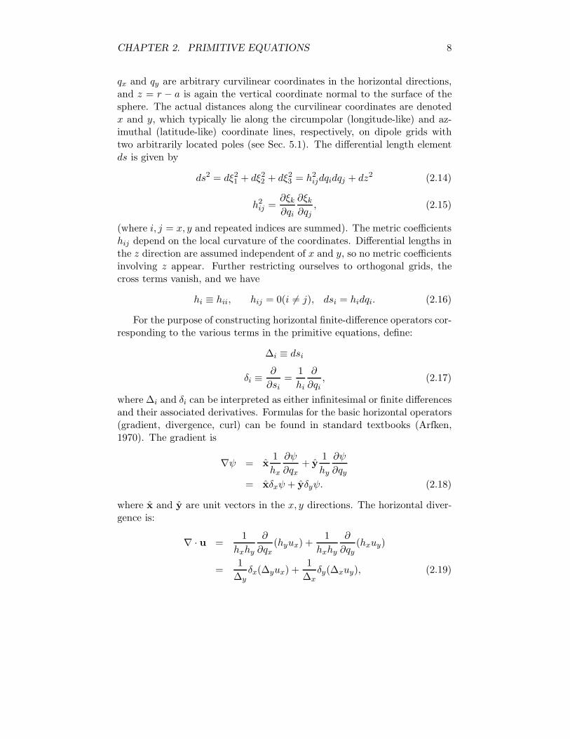
qx and qy are arbitrary curvilinear coordinates in the horizontal directions,and z = r − a is again the vertical coordinate normal to the surface of thesphere. The actual distances along the curvilinear coordinates are denotedx and y, which typically lie along the circumpolar (longitude-like) and az-imuthal (latitude-like) coordinate lines, respectively, on dipole grids withtwo arbitrarily located poles (see Sec. 5.1). The differential length elementds is given by
ds2 = dξ21 + dξ22 + dξ23 = h2ijdqidqj + dz2 (2.14)
h2ij =
∂ξk∂qi
∂ξk∂qj
, (2.15)
(where i, j = x, y and repeated indices are summed). The metric coefficientshij depend on the local curvature of the coordinates. Differential lengths inthe z direction are assumed independent of x and y, so no metric coefficientsinvolving z appear. Further restricting ourselves to orthogonal grids, thecross terms vanish, and we have
hi ≡ hii, hij = 0(i 6= j), dsi = hidqi. (2.16)
For the purpose of constructing horizontal finite-difference operators cor-responding to the various terms in the primitive equations, define:
∆i ≡ dsi
δi ≡∂
∂si=
1
hi
∂
∂qi, (2.17)
where ∆i and δi can be interpreted as either infinitesimal or finite differencesand their associated derivatives. Formulas for the basic horizontal operators(gradient, divergence, curl) can be found in standard textbooks (Arfken,1970). The gradient is
∇ψ = x1
hx
∂ψ
∂qx+ y
1
hy
∂ψ
∂qy= xδxψ + yδyψ. (2.18)
where x and y are unit vectors in the x, y directions. The horizontal diver-gence is:
∇ · u =1
hxhy
∂
∂qx(hyux) +
1
hxhy
∂
∂qy(hxuy)
=1
∆yδx(∆yux) +
1
∆xδy(∆xuy), (2.19)

CHAPTER 2. PRIMITIVE EQUATIONS 9
where ux and uy are the velocity components along the x and y directions.The advection operator (2.3) is similar:
L(α) =1
∆yδx(∆yuxα) +
1
∆xδy(∆xuyα) + δz(wα). (2.20)
The vertical component of the curl operator is
z · ∇ × u =1
hxhy
∂
∂qx(hyuy) −
1
hxhy
∂
∂qy(hxux)
=1
∆yδx(∆yuy) −
1
∆xδy(∆xux). (2.21)
Laplacian-type operators, which appear in the viscous and diffusive terms,have the form
∇ ·G∇ψ =1
∆yδx(∆yGδxψ) +
1
∆xδy(∆xGδyψ). (2.22)
where G is an arbitrary scalar function of x and y. Note that these operatorshave been expressed in terms of the differences and derivatives ∆i and δi, andhence there is no explicit dependence on the new coordinates qi or the metriccoefficients hi. In the discrete operators the same is true: it is not necessaryto have an analytic transformation with metric coefficients describing thenew coordinate system, it is only necessary to know the location of thediscrete grid points and the distances between neighboring grid points alongthe coordinate directions.
The other horizontal finite difference operators appearing in the primitiveequations can also be derived in general coordinates. The Coriolis terms aresimply given by
2Ω × u = −xfuy + yfux. (2.23)
The metric momentum advection terms corresponding to the third termson the left in (2.1) and (2.2) are given by Haltiner and Williams (1980) (p.442):
(uv tan φ)/a→ uxuyky − u2ykx (2.24)
(u2 tan φ)/a→ uxuykx − u2xky (2.25)
kx ≡ 1
hxhy
∂
∂qxhy =
1
∆yδx∆y (2.26)
ky ≡ 1
hxhy
∂
∂qyhx =
1
∆xδy∆x (2.27)

CHAPTER 2. PRIMITIVE EQUATIONS 10
Note that these revert to the standard forms (left of arrows) in spherical po-lar coordinates, where hx = a cosφ, hy = a, ux = u and uy = v. The metricterms in the viscous operators (second and third terms on the right in (2.4)and (2.5) require a more careful treatment. These terms were derived byWilliams (1972) in spherical coordinates, by applying the thin-shell approx-imation (r → a) to the viscous terms expressed as the divergence of a stresstensor whose components are linearly proportional to the components of therate-of-strain tensor. This form is transversely isotropic and ensures thatfor solid rotation the fluid is stress-free. The general coordinate versions ofthese terms are derived in Smith et al. (1995). The results are
FHx(ux, uy) = AM
∇2ux − ux(δxkx + δyky + 2k2
x + 2k2y)
+uy(δxky − δykx) + 2ky(δxuy) − 2kx(δyuy)
(2.28)
The formula for FHy(ux, uy) is the same with x and y interchanged every-where on the r.h.s. It is straightforward to show that these also reduce to thecorrect form in the spherical polar limit (2.4), (2.5). The above forms assumea spatially constant viscosity AM . More terms appear if AM is allowed tovary spatially. Wajsowicz (1993) derives the extra terms for spherical polarcoordinates. In general orthogonal coordinates they take the form:
FHx(ux, uy) = ∇ ·AM∇ux − ux
δxAMkx + δyAMky + 2AM (k2
x + k2y)
+uy(δxAMky − δyAMkx) (2.29)
+(2AMky + δyAM )(δxuy) − (2AMkx + δxAM )(δyuy).
The formula for FHy(ux, uy) is again the same with x and y interchangedeverywhere.
The general coordinate forms of the anisotropic and biharmonic viscousoperators are given in Sec. 7.2 below, and the Gent-McWilliams and bihar-monic forms of the horizontal diffusion terms are given in Sec. 7.1.
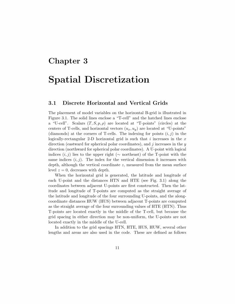
Chapter 3
Spatial Discretization
3.1 Discrete Horizontal and Vertical Grids
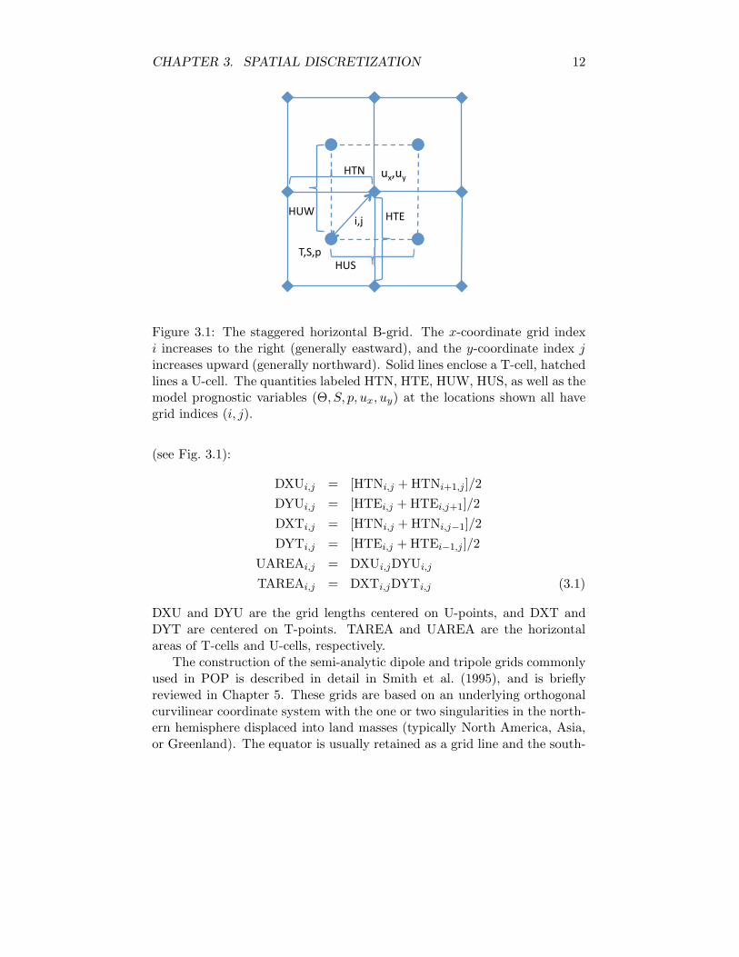
The placement of model variables on the horizontal B-grid is illustrated inFigure 3.1. The solid lines enclose a “T-cell” and the hatched lines enclosea “U-cell”. Scalars (T, S, p, ρ) are located at “T-points” (circles) at thecenters of T-cells, and horizontal vectors (ux, uy) are located at “U-points”(diamonds) at the corners of T-cells. The indexing for points (i, j) in thelogically-rectangular 2-D horizontal grid is such that i increases in the xdirection (eastward for spherical polar coordinates), and j increases in the ydirection (northward for spherical polar coordinates). A U-point with logicalindices (i, j) lies to the upper right (∼ northeast) of the T-point with thesame indices (i, j). The index for the vertical dimension k increases withdepth, although the vertical coordinate z, measured from the mean surfacelevel z = 0, decreases with depth.
When the horizontal grid is generated, the latitude and longitude ofeach U-point and the distances HTN and HTE (see Fig. 3.1) along thecoordinates between adjacent U-points are first constructed. Then the lat-itude and longitude of T-points are computed as the straight average ofthe latitude and longitude of the four surrounding U-points, and the along-coordinate distances HUW (HUS) between adjacent T-points are computedas the straight average of the four surrounding values of HTE (HTN). ThusT-points are located exactly in the middle of the T-cell, but because thegrid spacing in either direction may be non-uniform, the U-points are notlocated exactly in the middle of the U-cell.
In addition to the grid spacings HTN, HTE, HUS, HUW, several otherlengths and areas are also used in the code. These are defined as follows
11
CHAPTER 3. SPATIAL DISCRETIZATION 12
!" #$
%"&"'$
(")$
*%+$
*,&$
*%-$*,.$
Figure 3.1: The staggered horizontal B-grid. The x-coordinate grid indexi increases to the right (generally eastward), and the y-coordinate index jincreases upward (generally northward). Solid lines enclose a T-cell, hatchedlines a U-cell. The quantities labeled HTN, HTE, HUW, HUS, as well as themodel prognostic variables (Θ, S, p, ux, uy) at the locations shown all havegrid indices (i, j).
(see Fig. 3.1):
DXUi,j = [HTNi,j + HTNi+1,j]/2
DYUi,j = [HTEi,j + HTEi,j+1]/2
DXTi,j = [HTNi,j + HTNi,j−1]/2
DYTi,j = [HTEi,j + HTEi−1,j ]/2
UAREAi,j = DXUi,jDYUi,j
TAREAi,j = DXTi,jDYTi,j (3.1)
DXU and DYU are the grid lengths centered on U-points, and DXT andDYT are centered on T-points. TAREA and UAREA are the horizontalareas of T-cells and U-cells, respectively.
The construction of the semi-analytic dipole and tripole grids commonlyused in POP is described in detail in Smith et al. (1995), and is brieflyreviewed in Chapter 5. These grids are based on an underlying orthogonalcurvilinear coordinate system with the one or two singularities in the north-ern hemisphere displaced into land masses (typically North America, Asia,or Greenland). The equator is usually retained as a grid line and the south-
CHAPTER 3. SPATIAL DISCRETIZATION 13
!"!#$
%&$
%$
&'$
&($
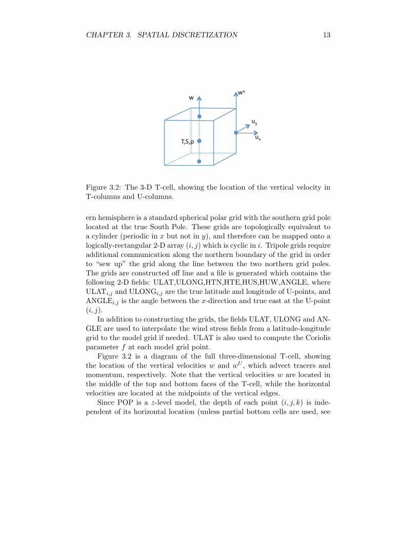
Figure 3.2: The 3-D T-cell, showing the location of the vertical velocity inT-columns and U-columns.
ern hemisphere is a standard spherical polar grid with the southern grid polelocated at the true South Pole. These grids are topologically equivalent toa cylinder (periodic in x but not in y), and therefore can be mapped onto alogically-rectangular 2-D array (i, j) which is cyclic in i. Tripole grids requireadditional communication along the northern boundary of the grid in orderto “sew up” the grid along the line between the two northern grid poles.The grids are constructed off line and a file is generated which contains thefollowing 2-D fields: ULAT,ULONG,HTN,HTE,HUS,HUW,ANGLE, whereULATi,j and ULONGi,j are the true latitude and longitude of U-points, andANGLEi,j is the angle between the x-direction and true east at the U-point(i, j).
In addition to constructing the grids, the fields ULAT, ULONG and AN-GLE are used to interpolate the wind stress fields from a latitude-longitudegrid to the model grid if needed. ULAT is also used to compute the Coriolisparameter f at each model grid point.
Figure 3.2 is a diagram of the full three-dimensional T-cell, showingthe location of the vertical velocities w and wU , which advect tracers andmomentum, respectively. Note that the vertical velocities w are located inthe middle of the top and bottom faces of the T-cell, while the horizontalvelocities are located at the midpoints of the vertical edges.
Since POP is a z-level model, the depth of each point (i, j, k) is inde-pendent of its horizontal location (unless partial bottom cells are used, see

CHAPTER 3. SPATIAL DISCRETIZATION 14
!
"#$!
%&' (!
%&)' (!
%&)'*(!
%&)'$(! &+' (! &)' (!
Figure 3.3: The vertical grid.
Sec. 5.2.2). The vertical discretization is illustrated in Figure 3.3. Thediscrete index k increases from the surface (k = 1) to the deepest level(k = km). The thickness of cells at level k is dzk. T-points are locatedexactly in the middle of each level, but because the vertical grid may benon-uniform (dzk 6= dzk+1), the interfaces where the vertical velocities w lieare not exactly halfway between the T-points. The vertical distances be-tween T-points dzwk are just the average dzwk = 0.5(dzk + dzk+1), exceptat the surface where dzw0 = 0.5dz1. The depth of a T-point at level k is ztk,and zwk is the depth of the bottom of cells at level k. Note that while thecoordinate z is positive upward, ztk and zwk are positive depths. Verticalprofiles of dzk are usually generated offline and read in by the code, butthere is an option for generating this profile internally. Usually dzk is smallin the upper ocean and increases with depth according to a smooth analyticfunction describing the thickness as a function of depth. This is necessaryin order to maintain the formal second-order accuracy of the vertical dis-cretization; if the vertical spacing changes suddenly the scheme reverts tofirst order accuracy (Smith et al., 1995).
The topography is defined in the T-cells, which are completely filled witheither land or ocean (except when optional partial bottom cells are used;see Sec. 5.2.2). Thus U-points lie exactly on the lateral boundaries betweenland and ocean, and w points lie exactly on the ocean floor. These boundaryvelocities are by default set to zero for no-slip boundary conditions, thoughcan be modified by parameterizations like the overflow parameterization
CHAPTER 3. SPATIAL DISCRETIZATION 15
(Sec. 8.4). Vertical velocities wU along the rims in the stair-step topographymay also be nonzero (see the discussion of velocity boundary conditions inSec. 3.4.1). The topography is determined by the 2-D integer field KMTi,j
which gives the number of open ocean points in each vertical column of T-cells. The KMT field is usually generated offline and read in from a file inthe code. Thus 0 ≤ KMT ≤ km, and KMT = 0 indicates a surface landpoint. In some situations the ocean depth in a column of U-points is needed,and this is defined by the field KMUi,j , which is just the minimum of thefour surrounding values of KMT:
KMUi,j = minKMTi,j,KMTi−1,j,KMTi,j−1,KMTi−1,j−1 (3.2)
The depths of columns of ocean T-points and U-points are given, respec-tively, by:
HT = zw(KMT) ,
HU = zw(KMU) . (3.3)
With partial bottom cells the depth of the deepest ocean cell in each columnhas variable thickness, and the above formulas are modified accordingly (seeSec. 5.2.2).
3.2 Finite-difference operators
The exact finite-difference versions of the differential operators can be eas-ily derived for the various types of staggered horizontal grids A,B,C,D,E(Arakawa and Lamb, 1977) given only the forms of the fundamental opera-tors: divergence, gradient, and curl for that type of mesh. POP employs aB-grid (scalars at cell centers, vectors at cell corners) while some OGCM’suse a C-grid (scalars at cell centers, vector components normal to cell faces).We will use standard notation (Semtner, 1986) for finite-difference deriva-tives and averages:
δxψ = [ψ (x+ ∆x/2) − ψ (x− ∆x/2)]/∆x (3.4)
ψx
= [ψ (x+ ∆x/2) + ψ (x− ∆x/2)]/2 , (3.5)
with similar definitions for differences and averages in the y and z directions.These formulas strictly apply for uniform grid spacing; where, for example,if ψ is a tracer located at T-points, then ψ (x+ ∆x/2) is located on the eastface of a T-cell. For nonuniform grid spacing, the above definitions should

CHAPTER 3. SPATIAL DISCRETIZATION 16
be interpreted such that variables lie exactly at T- or U-cell centers andfaces, as appropriate.
The fundamental operators on C-grids have the same form as (2.18)-(2.22). On B-grids the derivatives involve transverse averaging, and thefundamental operators are given by:
∇ψ = xδxψy
+ yδyψx
(3.6)
∇ · u =1
∆yδx∆yux
y+
1
∆xδy∆xuy
x(3.7)
z · ∇ × u =1
∆yδx∆yuy
y − 1
∆xδy∆xux
x(3.8)
∇ ·G∇ψ =1
∆yδx[∆yGδxψ
y]y+
1
∆xδy[∆xGδyψ
x]x. (3.9)
The gradient is located at U-points and the divergence, curl and Laplacianare located at T-points. In the Laplacian operator G must also be definedat U-points. The factors ∆x, ∆y inside the difference operators δx, δy arelocated at U-points and are given by DXU, DYU, respectively, while thefactors 1/∆x, 1/∆y outside the difference operators, as well as similar factorsin the denominators of the difference operators δx, δy, are evaluated at T-points. For example, the first term on the r.h.s. of the divergence (3.7) atthe T-point (i, j) is given by
0.5[DYUi,j(ux)i,j + DYUi,j−1(ux)i,j−1
−DYUi−1,j(ux)i−1,j − DYUi−1,j−1(ux)i−1,j−1]/TAREAi,j (3.10)
In POP (and in other Bryan-Cox models which use a B-grid formulation)all viscous and diffusive terms are given in terms of an approximate C-griddiscretization in order to ensure they will damp checkerboard oscillations onthe scale of the grid spacing (see Secs. 3.3.2, 7.1, and 7.2).
3.3 Discrete Tracer Transport Equations
The discrete tracer transport equations are:
∂
∂t(1 + ξ)ϕ+ LT (ϕ) = DH(ϕ) + DV (ϕ) + F
W(ϕ) (3.11)
where LT is the advection operator in T-cells, and DH , DV are the horizontaland vertical diffusion operators, respectively. The factor (1+ξ) is associatedwith the change in volume of the surface layer due to undulations of the free
CHAPTER 3. SPATIAL DISCRETIZATION 17
surface, and FW
(ϕ) is the change in tracer concentration associated withthe freshwater flux. ξ and F
W(ϕ) are given by
ξ =δk1
dz1η (3.12)
FW
(ϕ) =δk1
dz1
∑
m
q(m)W
ϕ(m)W
(3.13)
where δk1 is the Kronecker delta, equal to 1 for k = 1 and zero otherwise. ηis the displacement of the free surface relative to z = 0, q(m)
Wis the freshwater
flux per unit area associated with a specific source (labeled m) of freshwater.Thus, qW =
∑m q(m)
W= P −E+R−Fice +Mice is the total freshwater flux
per unit area associated with precipitation P , evaporation E, river runoff R,freezing Fice and melting Mice of sea ice, and ϕ(m)
Wis the tracer concentration
in the freshwater associated with source m. The change in volume of thesurface layer due to the freshwater flux is discussed in Sec. 4.5.1, and thenatural boundary conditions for tracers associated with freshwater flux arediscussed in Sec. 5.2.1. The boundary conditions on tracers are no-flux nor-mal to bottom and lateral boundaries, unless modified by parameterizationslike the overflow parameterization (see Sec. 8.4).
3.3.1 Tracer Advection
POP has multiple options for tracer advection. Here we describe a basicsecond-order centered advection scheme as an example of a discretization.Other advection schemes are described in Chapter 6. In the standard second-order scheme, the advection operator is given by:
LT (ϕ) =1
∆yδx(∆yux
yϕx) +
1
∆xδy(∆xuy
xϕy) + δz(wϕ
z) (3.14)
Again, ∆x and ∆y inside the difference operator are located at U-points,and the mass fluxes ∆yux
y, ∆xuy
xare located on the lateral faces of T-
cells. ϕx and ϕy are also located on the lateral faces of T-cells, while ϕz
is located on the top and bottom faces of T-cells. At the surface, ϕz is setequal to zero because there is no advection of tracers across the surface.The vertical velocity w at T-points is determined from the solution of thecontinuity equation
1
∆yδx(∆yux
y) +
1
∆xδy(∆xuy
x) + δz(w) = 0 (3.15)
CHAPTER 3. SPATIAL DISCRETIZATION 18
which is integrated in a column of T-cells downward from the top with theboundary conditions:
w =∂
∂tη + q
Wat z = 0 (3.16)
w = 0 at z = −HT . (3.17)
The boundary condition (3.16) is discussed in more detail in Sec. 4.5.1.When integrating from the top down using (3.15) and (3.16), the bot-
tom boundary condition (3.17) will only be satisfied to the extent that thesolution of the elliptic system of barotropic equations for the surface heightη has converged exactly (see Sec. 4.5). In practice, this exact convergenceis not achieved, so the bottom velocity in T-columns is set to zero to ensureno tracers are fluxed through the bottom. This amounts to allowing a verysmall divergence of velocity in the bottom cell.
In versions of POP prior to 1.4.3, the volume of the surface cells isassumed constant, and no account is taken of the change in volume of thesurface cells when the free surface height changes. Thus ξ = 0 and q
W= 0
in (3.11), (3.12) and (3.13), and the freshwater flux is approximated as avirtual salinity flux and imposed as a boundary condition on the verticaldiffusion operator. In addition, the tracers are advected through the surfacein this formulation using (3.14) with the vertical velocity given by (3.16) andϕz = ϕ1 at the surface. One problem with this approximation is that theadvective flux of tracers through the surface is not zero in global average.The globally integrated vertical mass flux vanishes, but the integrated tracerflux does not. In practice, we have found that the residual surface tracerfluxes associated with this are usually small, but in some situations they maybe non-negligible. (Note: the global mean residual surface tracer fluxes arestandard diagnostic model output in the earlier versions of POP without thevariable thickness surface layer.) Because the residual surface flux is nonzero,the global mean tracers are not conserved. In POP version 1.4.3, the surfacelayer is based on (3.11), (3.12) and (3.13), and global mean tracers (inparticular total salt) are conserved exactly. The variable-thickness surfacelayer is detailed in Sec. 5.2.1.
3.3.2 Horizontal Tracer Diffusion
POP has three options for horizontal tracer diffusion: 1) horizontal Lapla-cian diffusion, 2) horizontal biharmonic diffusion, 3) the Gent-McWilliamsparameterization, which includes along-isopycnal tracer diffusion and traceradvection with an additional eddy-induced transport velocity. All of these

CHAPTER 3. SPATIAL DISCRETIZATION 19
are implemented for a spatially varying diffusivity. The first of these options(Laplacian diffusion) is described here, the other two options are discussedin Sec. 7.1. The discrete horizontal Laplacian diffusion operator is given by:
DH(ϕ) =1
∆yδx(AH
x∆yδxϕ) +
1
∆xδy(AH
y∆xδyϕ) (3.18)
Note that no lateral averaging is involved as in (3.9). Thus the Laplacianis approximated as a five-point stencil as would be used on a C-grid. Thefactors ∆x, ∆y inside the difference operator are given by HTN, HTE, re-spectively (see Fig. 3.1), and AH , defined at T-points, is averaged acrossthe T-cell faces. As mentioned above, all the horizontal diffusive operatorsin POP that would normally involve nine-point operators (including theGM parameterization and the horizontal friction operators), are approxi-mated by five-point C-grid operators in order to ensure that they dampcheckerboard noise on the grid scale. B-grid Laplacian-type operators like(3.9) have a checkerboard null space, i.e., they yield zero when applied toa +/− checkerboard field, and thus cannot damp noise of this character(see Sec. 5.2.1). The only Laplacian-type operator which uses a B-grid dis-cretization is the elliptic operator in the implicit barotropic system. Therethe B-grid discretization is required in order to maintain energetic consis-tency (Smith et al., 1992; Dukowicz et al., 1993), see also Secs. 3.5 and 4.5).The boundary conditions on the diffusive operator (3.18) are that tracergradients δxϕ, δyϕ are zero normal to lateral boundaries.
3.3.3 Vertical Tracer Diffusion
The spatial discretization of the vertical diffusion operator is given by:
DV (ϕ) = δz(κδzϕ)
=1
dzk
(κk− 1
2
(ϕk−1 − ϕk)
dzk− 1
2
−κk+ 1
2
(ϕk − ϕk+1)
dzk+ 1
2
). (3.19)
where ϕk is a tracer at level k, and κk− 1
2
, κk+ 1
2
are evaluated on the top and
bottom faces, respectively, of the T-cell at level k, and dzk− 1
2
= dzwk−1,
dzk+ 1
2
= dzwk. The boundary conditions at the top and bottom of the
column are
κδzϕ→ Qϕ at z = 0
κδzϕ→ 0 at z = −HT (3.20)
CHAPTER 3. SPATIAL DISCRETIZATION 20
where Qϕ is the surface flux of tracer ϕ (e.g., heat flux for temperatureand equivalent salt flux associated with freshwater flux for salinity). Themodifications to this discretization when partial bottom cells are used isdescribed in Sec. 5.2.2. The diffusive term may either be evaluated explicitlyor implicitly. The implicit treatment is described in Sec. 4.2.2. With explicitmixing, a convective adjustment routine may also be used to more efficientlymix tracers when the column is unstable (see Sec. 7.3.1). Various subgrid-scale parameterizations for the vertical diffusivity are discussed in Sec. 7.3.
3.4 Discrete Momentum Equations.
The momentum equations discretized on the B-grid are given by:
∂
∂tux + LU (ux) + uxuyky − u2
ykx − fuy = − 1
ρ0
δxpy + FHx(ux, uy) + FV (ux)
(3.21)∂
∂tuy +LU (uy) + uxuykx − u2
xky + fux = − 1
ρ0
δypx +FHy(uy, ux) +FV (uy)
(3.22)In these equations no account has been taken of the change in volume of thesurface layer due to undulations of the free surface. Therefore, no terms in-volving ξ appear as in the tracer transport equation (3.11). The justificationfor this is that the global mean momentum, unlike the global mean tracers, isnot conserved in the absence of forcing, so there is less motivation to correctfor momentum nonconservation due to surface height fluctuations. Further-more, the error introduced is typically small compared to the uncertainty inthe applied wind stress.Note: Currently the code is in cgs units and it is assumed that ρ
0= 1.0g
cm−3, so it never explicitly appears. If the Boussinesq correction (Sec. 8.1.1)is used, then this factor is already taken into account, because the factorr(p) in (8.7) is normalized such that the pressure gradient should be dividedby ρ
0= 1.0.
3.4.1 Momentum Advection
The nonlinear momentum advection term is discretized as:
LU (α) =1
∆yδx[(∆yux
y)xyαx]+
1
∆xδy[(∆xuy
x)xyαy]+ δz(w
Uαz) . (3.23)
This is a second-order centered advection scheme and is currently the onlyoption available in POP for momentum advection. It has the property
CHAPTER 3. SPATIAL DISCRETIZATION 21
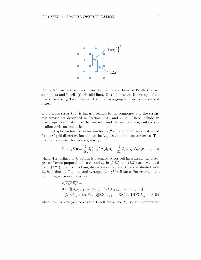
that global mean kinetic energy is conserved by advection. Momentumis conserved in the interior by advection, but not on the boundaries (seeSec. 3.5 on energetic consistency). The mass fluxes in the operator includean extra average in both horizontal directions, denoted (..)
xy. Both the
horizontal and vertical mass fluxes in a U-cell are the average of the foursurrounding T-cell mass fluxes. This is illustrated in Figure 3.4 for the massflux in the x-direction. As a consequence, the vertical velocity in a U-cellis exactly the area-weighted average of the four surrounding T-cell verticalvelocities w. This averaging is necessary in order to maintain the energeticbalance between the global mean work done by the pressure gradient and thechange in gravitational potential energy (Smith et al., 1992), see also Sec. 3.5on energetic consistency. An additional advantage of this flux averaging inU-cells is that it substantially reduces noise in the vertical velocity fieldcompared to other approaches (Webb, 1995). At the bottom of a column ofocean U-cells wU is not necessarily zero, because it is the weighted averageof the surrounding w’s, some of which may be nonzero if it is a “rim” pointwhere k = KMU but at least one of the surrounding T-points has k <KMT. It can be shown that the value of wU at these points approximatesthe boundary condition for tangential flow along the sloping bottom w =−u ·∇H (Semtner, 1986). Momentum is advected through the surface usingthe vertical velocity (3.16) averaged to U-points and with αz = α1 (whereα = ux or uy) in (3.23).
3.4.2 Metric Terms
The metric terms (third and fourth terms on the l.h.s. in 3.22) are con-structed using a simple C-grid discretization of the metric factors, as in(2.26) and (2.27). Specifically, kx and ky at U-points are:
KXUi,j = [HUWi+1,j − HUWi,j]/UAREAi,j
KYUi,j = [HUSi,j+1 − HUSi,j]/UAREAi,j (3.24)
3.4.3 Horizontal Friction
Several options for horizontal friction are available in the code. In thissection a simple spatial discretization of the Laplacian-type formulation witha spatially varying viscous coefficient as given by (2.30) is presented. Thebiharmonic friction operator obtained by applying (2.28) twice is describedin Sec. 7.2.2. More sophisticated formulations of the viscosity based on afunctional discretization of the friction operator formulated as the divergence
CHAPTER 3. SPATIAL DISCRETIZATION 22
u yx
( )xy
u yx
Figure 3.4: Advective mass fluxes through lateral faces of T-cells (narrowsolid lines) and U-cells (thick solid line). U-cell fluxes are the average of thefour surrounding T-cell fluxes. A similar averaging applies to the verticalfluxes.
of a viscous stress that is linearly related to the components of the strain-rate tensor are described in Sections 7.2.3 and 7.2.3. These include ananisotropic formulation of the viscosity and the use of Smagorinksy-typenonlinear viscous coefficients.
The Laplacian horizontal friction terms (2.28) and (2.30) are constructedfrom a C-grid discretization of both the Laplacian and the metric terms. Thediscrete Laplacian terms are given by:
∇ ·AM∇u =1
∆yδx(AM
x∆yδxu) +
1
∆xδy(AM
y∆xδyu) (3.25)
where AM , defined at U-points, is averaged across cell faces inside the diver-gence. Terms proportional to kx and ky in (2.28) and (2.30) are evaluatedusing (3.24). Terms involving derivatives of kx and ky are evaluated withkx, ky defined at T-points and averaged along U-cell faces. For example, theterm δxAMkx is evaluated as:
δxAMxkx
y=
0.25[(AM )i+1,j + (AM )i,j][KXTi+1,j+1 + KXTi+1,j]
−[(AM )i,j + (AM )i−1,j ][KXTi,j+1 + KXTi,j]/DXUi,j (3.26)
where AM is averaged across the U-cell faces, and kx, ky at T-points are
CHAPTER 3. SPATIAL DISCRETIZATION 23
given by
KXTi,j = [HTEi,j − HTEi−1,j]/TAREAi,j
KYTi,j = [HTNi,j − HTNi,j−1]/TAREAi,j (3.27)
Finally, in those terms in (2.28,2.30) that involve single derivatives of thevelocities or viscosities (e.g. δxuy or, δxAM ) the derivatives are evaluatedas differences across the cell without using the central value. For example,δxuy at point (i, j) is evaluated as:
[(uy)i+1,j − (uy)i−1,j ]/[HTNi,j + HTNi+1,j ] (3.28)
The no-slip boundary conditions are implemented by simply setting ux =uy = 0 on all lateral boundary points. Modifications to the operator whenpartial bottom cells are used are described in Sec. 5.2.2.
3.4.4 Vertical Friction
The spatial discretization of the vertical friction terms is essentially identicalto that of the vertical diffusion described in Sec. 3.3.3. The spatial discretiza-tion of both FV (ux) and FV (uy) is identical to (3.19) with κ replaced by thevertical viscosity µ and ϕ replaced by one of the velocity components ux oruy. Modifications for partial bottom cells are discussed in Sec. 5.2.2. Theboundary conditions at the top and bottom of the column of U-points are
µδz(ux, uy) → (τx, τy) at z = 0
µδz(ux, uy) → c|u|(ux, uy) at z = −HU (3.29)
where (τx, τy) are the components of the surface wind stress along the coor-dinate directions, and a quadratic drag term is applied at the bottom of thecolumn. The dimensionless constant c is typically chosen to be of order 10−3.The semi-implicit treatment of these terms is described in Sec. 4.4.2. Var-ious subgrid-scale parameterizations for the vertical viscosity are describedin Sec. 7.3.
3.5 Energetic Consistency
The energetic balances in the free-surface formulation are described in de-tail in Dukowicz and Smith (1994). However, this reference predates theimplementation of a variable-surface thickness layer (Sec. 5.2.1) and partialbottom cells (Sec. 5.2.2), both of which influence the energetic balances.

Chapter 4
Time Discretization
The POP model uses a three-time-level second-order-accurate modified leap-frog scheme for stepping forward in time. It is modified in the sense thatsome terms are evaluated semi-implicitly, and of the terms that are treatedexplicitly, only the advection operators are actually evaluated at the centraltime level, as in a pure leapfrog scheme. The diffusive terms are evaluatedusing a forward step. The reason for this is that the centered advectionscheme is unstable for forward steps, and the diffusive scheme is unstablefor leapfrog steps.
4.1 Filtering Timesteps
Leapfrog schemes can develop computational noise due to the partial decou-pling of even and odd timesteps. In a pure leapfrog scheme they are com-pletely decoupled and the solutions on the even and odd steps can evolveindependently, leading to 2∆t oscillations in time. There are several meth-ods to damp the leapfrog computational mode, two of which are currentlyimplemented in POP.
One is to occasionally take a forward step or an Euler forward-backwardstep, sometimes called a Matsuno timestep (Haltiner and Williams, 1980).The Matsuno step is a forward predictor step followed by a “backward”step which is essentially a repeat of the forward step but using the predictedprognostic variables from the first pass to evaluate all terms except the time-tendency term (see Sec. 4.2). The Matsuno step is more expensive than aforward step, but it is stable for advection.
The other method is to occasionally perform an averaging of the solutionat three successive time levels to the two intermediate times, back up half a
24
CHAPTER 4. TIME DISCRETIZATION 25
timestep and proceed. The later procedure is referred to as an “averagingtimestep” (Dukowicz and Smith, 1994) and is the recommended method foreliminating the leapfrog computational mode. The leapfrog scheme gener-ates two different “trajectories” of the solution, one corresponding to evenand one to odd steps. The advantage of the averaging step is that it placesthe solution on the average trajectory, whereas the forward and Matsunosteps select only one trajectory, corresponding to either the even or the oddsolution. Experience has shown that some model configurations are not sta-ble using Matsuno filtering timesteps, and this is especially true with thevariable-thickness surface layer (Sec. 5.2.1).
On the very first time step of a spinup from rest a forward step is takento avoid immediately exciting a leapfrog computational mode (this feature ishardwired into the code). In the presentation below, the time discretizationof various terms will first be presented for a regular leapfrog step, then thediscretization for the forward and backward steps will be given.
4.2 Tracer Transport Equations
Labeling the three time levels on a given step as n − 1, n, and n + 1, thetracer transport equation (3.11) is discretized in time as follows:
(1+ξn+1)ϕn+1−(1+ξn−1)ϕn−1 = τ [−L(n)T (ϕn)+DH(ϕn−1)+DV (ϕλ)+Fn
W]
(4.1)ϕλ = λϕ(n+1) + (1 − λ)ϕ(n−1) (4.2)
where ∆t is the timestep and τ = 2∆t. FnW
is given by (3.13) with qW
andϕ evaluated at time n, and ξn is given by (3.12) with η evaluated at time n.The superscript (n) on the advection operator indicates that the advectivemass fluxes are evaluated using the time n velocities. The vertical diffusionterm may be evaluated either explicitly or semi-implicitly. In the explicitcase λ = 0. For semi-implicit diffusion λ ≥ 1/2 is required for stability, andthe code is usually run with λ = 1. The surface forcing (3.20), applied as aboundary condition on the vertical diffusion operator, is evaluated at time nfor both explicit and semi-implicit mixing. The modifications to the tracertransport equations with implicit vertical mixing are described in Sec. 4.2.2.
With pressure averaging (see Sec. 4.4.1) the potential temperature andsalinity at the new time are needed to evaluate the pressure gradient at thenew time. This is required in the baroclinic momentum equations beforethe barotropic equations have been solved for the surface height at the newtime. Therefore, (4.1) cannot be used to predict the new tracers because

CHAPTER 4. TIME DISCRETIZATION 26
ξn+1 is not yet known. Instead an approximation is made to predict thenew temperature and salinity which are then used to evaluate the pressuregradient at the new time. After the barotropic equations have been solved,the new potential temperature and salinity are corrected so that they satisfy(4.1) exactly. The equations for predicting and correcting the tracers at thenew time are obtained as follows. The l.h.s. of (4.1), which involves theunknown surface height ηn+1, is approximated as:
(1 + ξn+1)ϕn+1 − (1 + ξn−1)ϕn−1 = (ϕn+1 − ϕn−1)+12
(ξn+1 + ξn−1
)(ϕn+1 − ϕn−1) + (ξn+1 − ξn−1)1
2
(ϕn+1 + ϕn−1
)
≈ (1 + ξn)(ϕn+1 − ϕn−1) + 2(ξn − ξn−1)ϕn (4.3)
With this approximation, the equations for predicting and correcting Θ andS are given by:Predictor:
(1 + ξn)(ϕn+1 − ϕn−1) = −2(ξn − ξn−1)ϕn + τF (4.4)
Corrector:
(1 + ξn+1)ϕn+1 = (1 + ξn)ϕn+1 + (ξn − ξn−1)(2ϕn − ϕn−1) (4.5)
where ϕn+1 is the predicted tracer at the new time, and F represents allterms in brackets on the r.h.s. of (4.1). Note that these equations are usedonly to predict and correct Θ and S; all passive tracers are updated directlyusing (4.1).
The time discretization for the two-time-level forward and backwardsteps is given byForward step:
(1 + ξ∗)ϕ∗ − (1 + ξn)ϕn = τ [−L(n)T (ϕn) + DH(ϕn) + DV (ϕλ) + Fn
W]
ϕλ = λϕ∗ + (1 − λ)ϕn (4.6)
Backward step:
(1 + ξn+1)ϕn+1 − (1 + ξn)ϕn = τ [−L(∗)T (ϕ∗) + DH(ϕ∗) + DV (ϕλ) + Fn
W]
ϕλ = λϕn+1 + (1 − λ)ϕn (4.7)
Here τ = ∆t and ϕ∗, the predicted tracer at the new time from the forwardstep, is used to evaluate the r.h.s. in the backward step. ξ∗ is given by (3.12)
with η = η∗. L(∗)T is the advection operator evaluated using the predicted
velocities from the forward step (see Sec. 4.4). For a forward step only,ϕ∗ = ϕn+1. The surface forcing applied to DV , as well as the freshwatertracer flux F
W, are evaluated at time n in both forward and backward steps.

CHAPTER 4. TIME DISCRETIZATION 27
4.2.1 Tracer Acceleration
The acceleration technique of Bryan (1984) can be used to more quickly spinup the model to a steady state by modifying the timestep for the momentumequation, or tracers in the deep ocean. The basic method is to modify thetime step τ as follows in the baroclinic and barotropic momentum equations:(4.20) and (4.39)
τ → τ(u)k = τ (u)/α (4.8)
and in the tracer transport equation (4.1)
τ → τ(ϕ)k = τ (ϕ)/γk (4.9)
where superscripts denote timesteps for the momentum and continuity (u),and tracers (ϕ). α and γk are acceleration factors specified in the namelistmodel input: dtuxcel = α−1, dttxcel(k) = (γk)
−1, in addition to the tracertimestep. Note that τ (u) is not a model input.
There are some points to make about the use of acceleration. First, adisadvantage of depth-dependent tracer acceleration is that it leads to non-conservative advective and diffusive fluxes when γk 6= γk+1. For this reason,it is recommended that profiles of γk be smooth functions of depth, and thatthe largest vertical discontinuities in γk be restricted to depths where fluxesare small enough that tracers are well conserved. The depth-dependenttracer timestep must also be accounted for in the convective adjustmentand vertical mixing routines. These changes are described in Secs. 7.3.1,4.2.3, and 4.4.2. Danabasoglu (2004) shows some detrimental effects of thetracer non-conservation with this type of acceleration method, includingthe model approaching an incorrect steady state solution. Therefore, it isrecommended that the depth-dependent tracer acceleration not be used.
Second, if α 6= γ1, then the surface forcing for momentum does not occurat the correct time because the model calender and forcing fields are basedon the surface tracer time step. For this reason, if momentum acceleration,α 6= 1, is used, then a subsequent synchronous integration is required to getthe momentum and tracer fields back in step. This acceleration techniqueis recommended by Danabasoglu (2004), who used a value of α = 5. Third,if the variable thickness surface layer option is used with virtual salt fluxboundary conditions, see Sec. 5.2.1, Danabasoglu (2004) shows the momen-tum acceleration technique is stable, despite the fact that the time steppingdiscretizations in the tracer transport and barotropic continuity equationsare inconsistent.
CHAPTER 4. TIME DISCRETIZATION 28
4.2.2 Implicit Vertical Diffusion
The tracer equations with implicit vertical diffusion involve the solutionof a tridiagonal system in each vertical column of grid points. This is arelatively easy thing to do because the system does not involve any couplingwith neighboring points in the horizontal direction. The equations solved inthe code are
[1 + ξn+1 − λτA(κ)]∆ϕ = −(ξn+1 − ξn−1)ϕn−1
+ τ [−L(n)T (ϕn) + DH(ϕn−1) + A(κ)ϕn−1 + Fn
W]
A(κ) = δzκδz , ∆ϕ ≡ ϕn+1 − ϕn−1 (4.10)
where τ = 2∆t. For explicit diffusion λ = 0, so the term in brackets on theright corresponds to the exact r.h.s. in the explicit case. The system is solvedfor the change in tracer ∆ϕ, subject to the no-flux boundary conditions
δz∆ϕ = 0 at both z = 0 and z = −HT . (4.11)
Note that because the surface forcing and freshwater tracer fluxes are eval-uated at time n, they are entirely contained in the r.h.s. of (4.10) and henceare not directly imposed as a boundary condition on the operator.
The predictor and corrector steps for updating Θ and S with pressureaveraging (Sec. 4.4.1) are given by:Predictor:
[1 + ξn − λτA(κ)]∆ϕ = −2(ξn − ξn−1)ϕn + τF
∆ϕ ≡ ϕn+1 − ϕn−1 (4.12)
Corrector:
[1 + ξn+1 − λτA(κ)]∆ϕ = (ξn − ξn−1)(2ϕn − ϕn−1) − (ξn+1 − ξn)ϕn+1
∆ϕ ≡ ϕn+1 − ϕn+1 (4.13)
where F represents all terms in brackets on the right-hand side of (4.10).These reduce to (4.4) and (4.5) in the limit λ = 0. Note that both thepredictor and corrector steps involve the solution of a tridiagonal system.
In forward and backward timesteps the implicit equations have the form:Forward step:
[1 + ξ∗ − λτA(κ)]∆ϕ = −(ξ∗ − ξn)ϕn
+ τ [−L(n)T (ϕn) + DH(ϕn) + A(κ)ϕn + Fn
W]
∆ϕ ≡ ϕ∗ − ϕn (4.14)
CHAPTER 4. TIME DISCRETIZATION 29
Backward step:
[1 + ξn+1 − λτA(κ)]∆ϕ = −(ξn+1 − ξn)ϕn
+ τ [−L(∗)T (ϕ∗) + DH(ϕ∗) + A(κ)ϕn + Fn
W]
∆ϕ ≡ ϕn+1 − ϕn (4.15)
where τ = ∆t.
4.2.3 Tridiagonal Solver
For the tridiagonal solution of (4.10), (4.12), (4.13), (4.14) or (4.15), a newalgorithm is used (Schopf and Loughe, 1995) which is more accurate andstable than traditional methods. These equations have the form:
(1 + ξ)Xk − λτkdzk
[ κk− 1
2
dzk− 1
2
(Xk−1 −Xk) −κk+ 1
2
dzk+ 1
2
(Xk −Xk+1)]
= Rk (4.16)
where Xk = ∆ϕ at level k, Rk is the r.h.s., and a depth-dependent timestep∆tk (τk = 2∆tk for leapfrog and τk = ∆tk for forward/backward timesteps)is used with tracer acceleration (see Sec. 4.2.1). Here ξ = ξn+1, except inthe predictor step (4.12) where ξ = ξn. (4.16) can be rewritten in the formof a tridiagonal system:
−AkXk+1 + CkXk − Ak−1Xk−1 = R′k (4.17)
Ak = λκk+ 1
2
dzk+ 1
2
Ck = h′k +Ak +Ak−1
R′k = hkRk
hk =dzkτk
h′k = hk(1 + ξ)
The algorithm for the solution of this system involves a loop over verticallevels to determine the coefficients:
Ek = Ak/Dk (4.18)
Fk = (R′k +Ak−1Fk−1)/Dk
where
Bk = Ak(h′k +Bk−1)/Dk
Dk = h′k +Ak +Bk−1
CHAPTER 4. TIME DISCRETIZATION 30
The loop begins at k = 1 with A0 = B0 = F0 = 0. This is followed byanother vertical loop to determine the solution by back substitution:
Xk = EkXk+1 + Fk (4.19)
This loop begins at the bottom with Xk+1 = 0 when k = KMT.
4.3 Splitting of Barotropic and Baroclinic Modes
The barotropic mode of the primitive equations supports fast gravity waveswith speeds of
√gH ∼ 200 m s−1. If resolved numerically, these waves
impose a severe restriction on the model timestep. However, they have littleeffect on the dynamics, especially on timescales longer than a day or so. Toovercome this severe limitation on the timestep, the barotropic mode is splitoff and solved as a separate 2-D system (see Sec. 4.5).
The barotropic equations are taken to be the vertically integrated mo-mentum and continuity equations. The true barotropic mode is not ex-actly isolated by the vertically integrated system, except in the limit ofa flat-bottom topography, a rigid lid, and a depth-independent buoyancyfrequency. Nevertheless, it suffices in practice to isolate and treat the verti-cally integrated system. Then, provided advective and diffusive CFL limitsdo not control the timestep, the baroclinic equations can be integrated witha timestep that is controlled by the gravity-wave speed of the first inter-nal mode, which is of order 2 m s−1, two orders of magnitude smaller thanthe barotropic wave speed. The procedure for solving the split barotropic-baroclinic system is as follows.
1) First the momentum equations are solved, without including the surfacepressure gradient, for an auxiliary velocity u′. This is what the momentumat the new time would be in the absence of the surface pressure gradient,which is depth-independent and hence determined only by the solution ofthe vertically integrated system. The time discretization of the resulting“baroclinic momentum equations” written in vector form is:
u′ − un−1
τ+ LU(un) − f z× uαγ = − 1
ρo∇ph + FH(un−1) + FV (uλ)(4.20)
where τ = 2∆t, LU represents the advection operator plus metric termsacting on both components of velocity, and FH and FV are now horizontalvectors. The overbars indicate various averages over the three time levels
CHAPTER 4. TIME DISCRETIZATION 31
for the semi-implicit treatment of the Coriolis, hydrostatic pressure gradient,and vertical mixing terms. The velocities are averaged as:
uαγ = αu′ + γun + (1 − α− γ)un−1 (4.21)
uλ = λu′ + (1 − λ)un−1 (4.22)
where α, γ, λ are coefficients used to vary the time-centering of the velocities.The averaging for the hydrostatic pressure ph is discussed in Sec. 8.1.2.To maintain an accurate time discretization of geostrophic balance, it isimportant that, in the averaging over the three time levels, the velocity andpressure are centered at the same time, i.e. if they are centered at time (n),then the coefficients for the variables at times (n + 1) and (n − 1) must beequal.
2) Next the vertical average of u′ is subtracted. The result is the baroclinicvelocity:
u′k = u′
k − 1
HU
km∑
k′=1
dzk′ u′k′ (4.23)
3) Finally, the barotropic system is solved for the barotropic velocity at thenew time Un+1 (see Sec. 4.5), and this is added to the normalized auxiliaryvelocities to obtain the full velocities at the new time:
un+1k = u′
k + Un+1 (4.24)
The barotropic velocity is defined by
U =1
H + η
∫ η
−Hdz u(z)
≈ 1
H
∫ 0
−Hdz u(z) =
1
HU
km∑
k=1
dzk uk . (4.25)
where η is the displacement of the free surface relative to z = 0. As discussedin Secs. 4.5 and 5.2.1, in the current version of the POP model we assumeη ≪ dz1 and approximate the barotropic velocity as the vertical integralfrom z = −H to z = 0 in (4.25).
CHAPTER 4. TIME DISCRETIZATION 32
4.4 Baroclinic Momentum Equations
The time discretization of the baroclinic momentum equations for leapfrogsteps is given by (4.20). For forward and backward steps, the time dis-cretization isForward steps:
u′∗ − un
τ+ LU(un) − f z× uθ = − 1
ρo∇pn
h + FH(un) + FV (uλ′
)
uθ = θu′∗ + (1 − θ)un
uλ′
= λ′u′∗ + (1 − λ′)un (4.26)
Backward steps:
u′ − un
τ+ LU(u′∗) − f z× uθ = − 1
ρo∇p∗h + FH(u′∗) + FV (uλ′
)
uθ = θu′ + (1 − θ)un
uλ′
= λ′u′ + (1 − λ′)un (4.27)
where τ = ∆t, and p∗h is the predicted hydrostatic pressure from the forwardstep. u′ is the unnormalized momentum, as in (4.20) and (4.23), and u′∗ isthe same quantity predicted by the forward step only. θ = 0.5 is hardwiredinto the code. This choice was made (rather than choosing θ = 0 whereboth Coriolis and pressure gradient would be centered and time n) becausethe forward step is unstable if the Coriolis terms is treated explicitly.
4.4.1 Pressure Averaging
The method of Brown and Campana (1978) is used for the semi-implicittreatment of the hydrostatic pressure gradient on leapfrog timesteps, wherethe averaging of the pressure over the three time levels in (4.20) is given by
1
ρo∇ph =
1
ρo∇(
1
4pn+1 +
1
2pn +
1
4pn−1) (4.28)
This choice of coefficients allows for a factor of two increase in the CFL limitassociated with internal gravity waves, and hence a factor of two increasein timestep if internal gravity waves are the controlling factor (see Maltrudet al., 1998, for a simple proof of this property).
The new pressure at time (n + 1) is obtained by updating the tracertransport equations for the temperature Θ and salinity S before the baro-clinic momentum equations are solved. Then the density and hydrostatic
CHAPTER 4. TIME DISCRETIZATION 33
pressure at the new time can be diagnosed from the equation of state and thehydrostatic equation. The convective adjustment is done afterwards and thismodifies the new Θ and S and hence the new pressure. So, in this case thenew pressure before convective adjustment is used in (4.28). With implicitvertical mixing the vertical loops over tracer and momentum are separated,and the implicit vertical diffusion of tracers is done after the tracer loopand before the momentum loop, so in that case the exact pressure at thenew time is used in (4.28). Equation (4.28) applies to leapfrog timesteps.On forward steps the time n pressure is used, and on backward steps thepredicted pressure from the first pass is used (see (4.26), (4.27)).
4.4.2 Semi-Implicit Treatment of Coriolis and Vertical Fric-tion Terms
A semi-implicit treatment of the Coriolis terms can allow a somewhat longertimestep due to filtering of inertial waves and barotropic Rossby waves, butthe main motivation in POP is to damp the Rossby-wave computationalmode which appears in the implicit free-surface formulation of the barotropicequations, as shown in Sec. 4.5 and Dukowicz and Smith (1994). Sincethe barotropic equations are the exact vertical average of the momentumequations, the Coriolis terms in the baroclinic equations must also be treatedsemi-implicitly. While it is possible to run POP with explicit treatmentof the Coriolis terms, we strongly recommend against this because of theabove-mentioned computational mode. The following discussion assumesthe Coriolis terms are treated semi-implicitly.
The simultaneous semi-implicit treatment of both Coriolis and verticalmixing terms leads to a coupled system where both components of velocitymust be solved for simultaneously. To avoid this, we employ an operatorsplitting which maintains the second-order accuracy of the time discretiza-tion. To illustrate this splitting, we write the momentum equations in thematrix form
u′ − un−1 + τBuαγ = τF + τA(µ)uλ (4.29)
τ = 2∆t, u =
(ux
uy
), B =
(0 −ff 0
), A(µ) = δzµδz
where u is the velocity vector organized in block form and B is a 2×2 matrixin the space of the two velocity components. F represents all other termsin the momentum equation that are treated explicitly (advection, metric,pressure gradient and horizontal diffusion terms). The time-averaging of

CHAPTER 4. TIME DISCRETIZATION 34
the velocities uαγ and uλ are given by (4.21) and (4.22). Equation (4.29)can be rewritten as
[I − λτA(µ) + ατB]∆u = τF′
F′ ≡ F − B[γun + (1 − γ)un−1] + A(µ)un−1∆u ≡ u′ − un−1 (4.30)
where I is the identity matrix. The operator splitting is given by
[I − λτA(µ) + ατB] = [I + ατB][I − λτA(µ)] + O(τ2) (4.31)
and thus second-order accuracy in time is maintained by dropping the O(τ2)terms and solving the simpler system
[I − λτA(µ)]∆u = (I + ατB)−1τF′ (4.32)
The r.h.s. of (4.32) can be evaluated analytically using
(I + ατB)−1 =1
1 + (ατf)2(I − ατB) . (4.33)
Note again that the surface forcing is contained only on the r.h.s. of (4.32).Furthermore, the quadratic bottom drag term (3.29) is evaluated at thelagged time (n− 1) and also appears only on the r.h.s. By lagging the bot-tom drag term, the tridiagonal systems for ux and uy are linearized and de-coupled, which greatly facilitates their solution. Again, λ = 0 is the explicitvertical mixing case. For implicit vertical mixing, λ > 0.5 is required, andthe code is typically run with λ = 1. In the barotropic equations (Sec. 4.5)we choose α = γ = 1/3, which is hardwired in the code, and it is clear from(4.21) that the Coriolis terms are centered at time n.
On forward and backward steps the splitting is given byForward step:
u′∗ − un + τBuθ = τF + τA(µ)uλ′
or
[I − λ′τA(µ) + θτB]∆u = τ [Fn − Bun + A(µ)un]
∆u ≡ u′∗ − un (4.34)
Backward step:
u′ − un + τBuθ = τF + τA(µ)uλ′
or
[I − λ′τA(µ) + θτB]∆u = τ [F∗ − Bun + A(µ)un]
∆u ≡ u′ − un (4.35)
CHAPTER 4. TIME DISCRETIZATION 35
where τ = ∆t, Fn represents the advection and hydrostatic pressure gradientterms evaluated at time n, and F∗ represents the same terms evaluated usingthe predicted variables from the forward step. In (4.34) and (4.35) uλ′
isdefined as in (4.26) and (4.27), respectively. Now employing the operatorsplitting
[I − λ′τA(µ) + θτB] = [I + θτB][I− λ′τA(µ)] + O(τ2) (4.36)
the tridiagonal systems analogous to (4.32) are:Forward step:
[I − λ′τA(µ)]∆u = (I + θτB)−1τ [Fn − Bun + A(µ)un]
∆u ≡ u′∗ − un (4.37)
Backward step:
[I − λ′τA(µ)]∆u = (I + θτB)−1τ [F∗ − Bun + A(µ)un]
∆u ≡ u′ − un (4.38)
Again, θ = 0.5 is hardwired into the code.
4.5 Barotropic Equations
POP uses the implicit free-surface formulation of the barotropic equationsdeveloped by Dukowicz and Smith (1994), and this formulation is pre-sented here. Other possible options are the rigid-lid streamfunction ap-proach (Bryan, 1969), the rigid-lid surface pressure approach (Smith et al.,1992; Dukowicz et al., 1993), and the explicit free-surface method (Killworthet al., 1991), which involves subcycling the barotropic mode with a smallertimestep than that used in the baroclinic equations.
The prognostic equation for the barotropic velocity, defined by (4.25), isobtained by vertically integrating the momentum and continuity equations.The barotropic momentum equation in block form, analogous to (4.29), isgiven by:
Un+1 − Un−1 + τBUαγ
= −τg∇ηαγ + τFB
Uαγ
= αUn+1 + γUn + (1 − α− γ)Un−1
ηαγ = αηn+1 + γηn + (1 − α− γ)ηn−1 (4.39)
where η = ps/ρ0g is the surface height, and FB is the vertical integral of
all terms besides the time-tendency, Coriolis, and surface pressure gradientterms in the momentum equation.

CHAPTER 4. TIME DISCRETIZATION 36
4.5.1 Linear Free Surface Model
A prognostic equation for the free surface height η is obtained by verticallyintegrating the continuity equation
∫ η
−Hdz(∇ · u +
∂w
∂z) =
∂
∂tη + ∇ · (H + η)U − q
W= 0, (4.40)
where we have used the surface boundary condition on the vertical velocity:
w(η) = dη/dt − qW
=∂
∂tη + u(η) · ∇η − q
W, (4.41)
and U is the vertically averaged horizontal velocity:
U =1
H + η
∫ η
−Hdzu(z) (4.42)
where w(η) and u(η) are the vertical and horizontal velocities at the surface,and q
Wis freshwater flux. This result is derived using Leibnitz’s Theorem
to interchange the order of integration and differentiation. A difficulty withthis form of the barotropic continuity equation is that, in the implicit timediscretization of the barotropic equations, the term proportional to η insidethe divergence in (4.40) leads to a nonlinear elliptic system, and standardsolution methods such as conjugate gradient algorithms cannot be directlyapplied to it. To avoid this, POP uses a linearized form of the barotropiccontinuity equation which is derived as follows. Integrating the continuityequation over depth as before, but modifying the boundary condition (4.41)by dropping the term involving ∇η (which can be shown to be of order|η|/dz1 relative to the time tendency term), we find:
∫ η
−Hdz(∇ · u +
∂w
∂z) =
∂
∂tη + ∇ ·HU +
∫ η
0dz∇ · u− q
W= 0 (4.43)
w(η) =∂
∂tη − q
W(4.44)
U =1
H
∫ 0
−Hdzu(z) (4.45)
To obtain the linearized barotropic continuity equation we drop the term∫ η0 dz ∇ · u in (4.43), which corresponds to neglecting the horizontal mass
flux between z = 0 and z = η:
∂
∂tη + ∇ ·HU = q
W. (4.46)

CHAPTER 4. TIME DISCRETIZATION 37
This derivation makes it clear that in the advection operators the horizontalmass flux between z = 0 and z = η must be neglected in order to beconsistent with (4.46). So there are four ingredients to the linear free surfacemodel: 1) the barotropic continuity equation is given by (4.46) instead of(4.40); 2) the barotropic velocity is given by (4.45) instead of (4.42); 3) thevertical velocity at the surface, which is used to integrate the continuityequation from the top down, is given by (4.44) instead of (4.41); and 4) thehorizontal mass fluxes between z = 0 and z = η should be neglected in theadvection operators and when integrating the continuity equation to find thevertical velocities. In the discrete equations this means that the horizontalmass fluxes in the surface cells are proportional to the full cell height dz1,rather than dz1 + η (see Sec. 5.2.1). This linear approximation is validprovided the surface displacement is small compared to the depth of thefull ocean: |η| ≪ H, and in the discrete equations the surface displacementmust also be small compared to the depth of the surface layer: |η| ≪ dz1.
With a non-zero freshwater flux qW
the mean volume of the ocean is notconstant, even though the velocity field is divergence free. Integrating (4.46)over horizontal area, we find
d
dt
∫dV =
∫da
∂
∂tη =
∫da q
W(4.47)
where da = dxdy is the horizontal area element. So the total volume of theocean will change unless the surface-integrated freshwater flux vanishes.
4.5.2 Time Discretization of the Barotropic Equations
In the implicit free-surface formulation the continuity equation (4.46) isdiscretized in time using a forward step as follows:
ηn+1 − ηn
∆t+ ∇ ·HU
α′
= qnW
Uα′
= α′Un+1 + (1 − α′)Un (4.48)
where α′ is a coefficient used to vary the time centering of the velocity inthe continuity equation. The barotropic equations support three types oflinear waves: two gravity waves (one in each horizontal direction) and oneRossby wave. In a pure leapfrog discretization, there would be three com-putational modes, one associated with each of these waves. By choosing theforward discretization (4.48), one computational mode is eliminated, leav-ing one gravity-like and one Rossby-like computational mode. The Rossby
CHAPTER 4. TIME DISCRETIZATION 38
computational mode is damped by the discretization scheme if the Coriolisterms are treated implicitly, and the gravity-wave computational mode isstrongly damped if α′ is close to 1. In Dukowicz and Smith (1994) it wasshown that the optimal set of time-centering coefficients which maximallydamps the computational modes, minimally damps the physical modes, andminimally distorts the phase speed of the physical modes is given by theparameter set:
α = γ =1
3, α′ = 1. (4.49)
Thus in (4.39)
ηαγ =1
3(ηn+1 + ηn + ηn−1)
and similarly for uαγ . These choices are hardwired into the code. Thephysical gravity waves are damped at small space and time scales in thisimplicit scheme, but the physical Rossby waves are essentially unaffected.
By inserting the barotropic momentum equation (4.39) into the continu-ity equation (4.48) we obtain an elliptic equation for the surface height atthe new time ηn+1. However, due to the presence of the Coriolis terms, theresulting elliptic operator is not symmetric, making it much more difficult toinvert, because standard solvers such as conjugate gradient methods requiresymmetric positive-definite linear operators. This problem can be overcomeby using an operator splitting technique that maintains the second-orderaccuracy of the time discretization scheme (Smith et al., 1992; Dukowiczet al., 1993). Defining an auxiliary velocity
U ≡ Un+1 + ατg∇(ηn+1 − ηn−1) (4.50)
equation (4.39) can be written:
(I + ατB)(U − Un−1) = τFB − B[γUn + (1 − γ)Un−1]
− g∇[γηn + (1 − γ)ηn−1] + O(fτ3) (4.51)
Dropping the O(fτ3) terms (which are the same order as the time truncationerror in this second-order scheme), and using the continuity equation (4.48)with α′ = 1, we arrive at the elliptic system
[∇ ·H∇− 1
gατ∆t
]ηn+1 = ∇ ·H
[ U
gατ+ ∇ηn−1
]− ηn
gατ∆t−
qnW
gατ(4.52)
The procedure is to first solve (4.51) for U, then solve (4.52) for ηn+1 (POPactually solves for the surface pressure ps = ρ
0gη), and finally use (4.50)
CHAPTER 4. TIME DISCRETIZATION 39
to obtain Un+1. This system is solved in POP on leapfrog timesteps withα = 1/3 using a diagonally preconditioned conjugate gradient algorithmdescribed in Sec. 4.5.3. Note that the terms dropped in (4.51) are onlyO(τ3) if the timestep is small compared to the inertial period 1/f . Wetherefore recommend that the model timestep be no greater than about twohours. The scheme is stable for longer timesteps, but the barotropic modewill start to become inaccurate as the timestep is increased above two hours.The divergence on the r.h.s. in (4.52) is discretized with the correct B-griddiscretization, i.e., the quantity in brackets is transversely averaged as in(3.7). The Laplacian-like operator on the l.h.s. in (4.52) is a nine-pointstencil with the correct B-grid discretization:
∇ ·H∇η =1
∆yδx[∆yHUδxηy
]y+
1
∆xδy[∆xHUδyηx
]x. (4.53)
Unlike the friction and diffusion operators, this operator cannot be approx-imated as a five-point stencil, because doing so would violate the energeticbalance between pressure work and change in potential energy (see Sec. 3.5).Since the nine-point B-grid operator in (4.53) has a checkerboard null space(see Sec. 5.2.1), the solution of (4.52) is prone to have local patches ofcheckerboard noise. Strictly speaking, the operator on the l.h.s. of (4.52)has no checkerboard null space due to the presence of the extra diagonalterm (second term in brackets). However, if the solution in some region isin a near steady state, this diagonal term is cancelled by the next to lastterm on the r.h.s., and checkerboard noise may appear. This is particularlytrue in isolated bays where the solution is only weakly coupled to the in-terior. On the other hand, the checkerboard noise has little effect on thedynamics because only the gradient of surface height enters the barotropicmomentum equation, and the B-grid gradient operator (3.6) does not seea checkerboard field. The only way a checkerboard surface height field canaffect the dynamics is through the vertical velocity at the surface (3.16),which depends on the change in surface height, and is used as the surfaceboundary condition to integrate the continuity equation to find the advec-tion velocities. However, experience has so far shown that this does not leadto serious problems with the model simulations.
It should be noted that the solution for surface height will only satisfythe continuity equation (4.48) to the extent that the solution of (4.52) hasconverged in the iterative solution of the elliptic solver. As discussed inSec. 3.3.1, this can lead to a small non-divergent mass flux in the bottom-most ocean cell when the 3-D continuity equation is integrated from the topdown with w given by (4.44) at the surface, as discussed in Sec. 3.3.1. In
CHAPTER 4. TIME DISCRETIZATION 40
practice, we suggest that the convergence criterion for the iterative solver bechosen so that the global mean balance between pressure work and changein potential energy is accurate to within about three significant digits (seeSec. 3.5 on energetic consistency).
The time discretization for forward and backwards steps, correspondingto (4.39) and (4.48) are given by:Forward step:
U∗ − Un + τBUθ
= −τg∇ηθ + τFnB
η∗ − ηn
∆t+ ∇ ·HU∗ = qn
W
Uθ
= θU∗ + (1 − θ)Un
ηθ = θη∗ + (1 − θ)ηn (4.54)
Backward step:
Un+1 − Un + τBUθ
= −τg∇ηθ + τF∗B
ηn+1 − ηn
∆t+ ∇ ·HUn+1 = qn
W
Uθ
= θUn+1 + (1 − θ)Un
ηθ = θηn+1 + (1 − θ)ηn (4.55)
where we have assumed α′ = 1 as in (4.48) and (4.49). U∗ and η∗ arethe predicted barotropic velocity and surface height from the forward step.Fn
B contains all terms other than the Coriolis, surface pressure gradient andtime-tendency terms in the barotropic momentum equation, all evaluated attime n, and F∗
B contains the same terms but evaluated using the prognosticvariables predicted by the forward step. The operator splittings for theforward and backward steps, analogous to (4.50) and (4.51) are:Forward step:
U ≡ U∗ + θτg∇(η∗ − ηn)
(I + θτB)(U− Un) = τFnB − Bun − g∇ηn + O(fτ3) (4.56)
Backward step:U ≡ Un+1 + θτg∇(ηn+1 − η∗)
(I+θτB)(U−Un) = τF∗B −Bun−g[θ∇η∗+(1−θ)∇ηn]+O(fτ3) (4.57)
Finally, the elliptic equations for the forward and backward steps analogousto (4.52) are given by:

CHAPTER 4. TIME DISCRETIZATION 41
Forward step:
[∇ ·H∇− 1
gθτ∆t
]η∗ = ∇ ·H
[ U
gθτ+ ∇ηn
]− ηn
gθτ∆t−qn
W
gθτ(4.58)
Backward step:
[∇ ·H∇− 1
gθτ∆t
]ηn+1 = ∇ ·H
[ U
gθτ+ ∇η∗
]− ηn
gθτ∆t−qn
W
gθτ(4.59)
4.5.3 Conjugate Gradient Algorithm
The most efficient method we have found for solving the elliptic system ofbarotropic equations (4.52) is to use a standard Preconditioned ConjugateGradient solver. The algorithm consists of the following steps to solve thesystem Ax = b given by (4.52) multiplied by the T-cell area. A is thesymmetric positive-definite Laplacian type operator on the l.h.s. in (4.52)(it is important to note that if (4.52) is not multiplied by the T-cell areathen the operator is not symmetric), b is the r.h.s., and x is the solution.Lower-case Greek and Roman letters are used, respectively for scalars and2-D arrays, and (x, y) denotes a dot product: (x, y) =
∑ij xijyij.
PCG Algorithm:
Initial guess: xo
Compute initial residual ro = b−Axo
Set βo = 1, so = 0For k = 1, 2, ..., kmax do
r′k−1 = Zrk−1
βk = (rk−1, r′k−1)
sk = r′k−1 + (βk/βk−1)sk−1
s′k = Ask (4.60)
αk = βk/(sk, s′k)
xk = xk−1 + αksk
rk = rk−1 − αks′k (4.61)
Exit if converged: (rk, rk)1
2 < ǫaEnd do

CHAPTER 4. TIME DISCRETIZATION 42
Here Z is a preconditioning matrix. This is usually taken to be a diagonalpreconditioner Z = C−1
0 , where C0 is the diagonal matrix composed of thecentral coefficient in the nine-point stencil corresponding to the operatorin (4.52). The code is set up to use a more sophisticated preconditionerconsisting of a nine-point operator which is a local approximate inverse ofthe true operator (Smith et al., 1992). This preconditioner is expensive tocompute but is time independent and can be computed offline and read inby the code. To improve the initial guess, xo is linearly extrapolated intime from the solutions at the two previous timesteps. In the convergencecriterion (rk, rk)
1
2 < ǫa, a is the rms T-cell area. This normalization issomewhat arbitrary, but is chosen so that ǫ has the same dimensions as theoperator (4.52) before it is multiplied by the T-cell area averaged over surfaceocean points. As discussed in Sec. 4.5.2, we suggest that ǫ be chosen suchthat the global mean balance between pressure work and change in potentialenergy is accurate to within about three significant digits. Typically this isachieved for values of ǫ between 10−12 and 10−13.
The conjugate gradient solver outlined above has poor scalability onmany distributed memory computer systems. The fundamental limit toscalability is the need for three dot products, each requiring a global sum-mation operation and adding an inherent sychronization. A variant of thestandard conjugate gradient solution method, known as the Chronopoulos-Gear algorithm (D’Azevedo et al., 1993), combines the separate global sumsinto a single vector global sum, which reduces the latency to one third. Thisoption is now the default in POP, though the previous PCG algorithm isstill supported.
Chapter 5
Grids
5.1 Global Orthogonal Grids
As discussed in Sec. 3, the POP model is designed to handle any orthogonalcurvilinear coordinate system for the horizontal grid. The only informationthe code needs locally at each grid point is the longitude and latitude ofvelocity points and the distances to neighboring points along the two coor-dinate directions. This information is computed offline and read in from afile. However, there are restrictions on the global connectivity of the grid.In the current model release, it is assumed that the computational grid canbe mapped onto a 2-D domain. When such global grids are mapped ontothe sphere they necessarily involve two singularities, analogous to the northand south poles on a standard polar grid. In these “dipole” grids, originallydeveloped independently by two groups (Madec and Imbard, 1996; Smithet al., 1995), the two singularities can be placed inside land masses (e.g.,North America, Greenland or Asia) to construct global grids. POP also hasthe ability to use what we call “tripole” grids, which were originally devel-oped by Murray (1996). In these grids, there are two “poles” in the northernhemisphere (usually placed in North America and Asia). These grids canalso be mapped onto a cylinder but special boundary communications arerequired in order to “sew up” the line between the two northern poles. Inboth dipole and tripole grids, the meshes are constructed so that there is asmooth transition moving north from the Equator, from the southern hemi-sphere polar grid (usually Mercator grid) to the northern “distorted” grid.Various factors enter into the design of a given grid, and different choices(pole locations, dipole vs. tripole) may be preferred for different problems.In global grids the Equator is typically chosen as a grid line so that the nu-
43
CHAPTER 5. GRIDS 44
merical dispersion relation for the B-grid linear Kelvin waves is accurate. Atresolutions coarser than about 1
2
, the meridional spacing near the Equator is
enhanced (to about 12) in order to more accurately resolve equatorial waves
and currents. Note: Software for generation of global dipole and tripolegrids is not released with the code, but will eventually be made public.
5.1.1 Dipole Grids
The simplest orthogonal grid with two arbitrarily located poles can be con-structed analytically in one of three ways:
1. Electrostatic dipole charge distribution on a sphere: solve Poisson’sEquation on the sphere with two electric charges of opposite sign atthe chosen pole points; the electric field lines and the lines of constantelectrostatic potential form an orthogonal coordinate system;
2. Conformal map method (Murray, 1996): project a spherical polar gridonto a tangent plane at its equator from the point on the sphere oppo-site the tangent point, then reproject back onto a larger sphere tangentto the plane at the same point; the new pole points on the larger spherewill be shifted toward its equator and the tangent point;
3. Geometric method (Smith et al., 1995): choose two axes, one whichintersects the surface of the sphere at the two pole points and onelocated at the intersection of the two planes tangent to the pole points,then the two families of planes that contain these axes intersect thesurface of the sphere in two sets of circles which form the coordinatesof an orthogonal coordinate system.
All these methods produce equivalent orthogonal grids. The only problemwith these simple analytic grids is that if one pole is located in Antarcticaand the other is displaced away from the true North Pole, then the Equatorwill not be a grid line. To get around this problem, grids can be con-structed by an iterative procedure (Madec and Imbard, 1996; Smith et al.,1995), starting at the equator of a southern hemisphere polar grid, where thenorthern pole point is gradually shifted away from the true North Pole assuccessive latitude-like circles are constructed. In this manner it is possibleto construct a semi-analytic dipole grid which smoothly matches onto thesouthern polar grid, and in which local changes in grid spacing are every-where small and smooth. Composite grids that have sudden changes in gridspacing normal to matching boundaries suffer a loss of formal second-orderaccuracy of the spatial discretization scheme (Smith et al., 1995).

CHAPTER 5. GRIDS 45
Figure 5.1: A dipole grid.
An example of a semi-analytic dipole grid is shown in Figure 5.1. In thisgrid the northern pole is in North America and the southern hemisphere is aMercator grid with a pole at the true South Pole. Note that the meridionalgrid spacing near the Equator has been enhanced as discussed above. Thegrid spacing in the northern hemisphere is chosen so as to minimize theglobal mean aspect ratio, attempting to make each cell as nearly “square”as possible (as in a true Mercator grid). In both hemispheres the gridterminates in a circle enclosing the pole, and anything within this circle isexcluded (e.g., Hudson Bay in Fig. 5.1).
5.1.2 Tripole Grids
Analytic grids can also be constructed which involve more than two singu-larities using the different methods described above for dipole grids. Varioustypes of multipole grids are discussed by Murray (1996). One variation thatis particularly useful for ocean models is shown in Figure 11 of Murray

CHAPTER 5. GRIDS 46
(1996). It has two singularities in the northern hemisphere and smoothlymatches onto a southern hemisphere Mercator grid. A “tripole” grid of thistype is shown in Figure 5.2. Note that the grid spacing in the Arctic is muchmore uniform and the cell aspect ratios are much closer to one than in thedipole grid in Figure 5.1. This particular grid was constructed for the FrenchOPA model (Madec et al., 1998), and was made available, courtesy of G.Madec, for testing in POP. Like the dipole grid, the tripole grid is mappedonto a cylinder (a logical 2-D array that is periodic in the x direction). Thedifference is that in the dipole grid the northernmost (“upper”) boundaryof the grid corresponds to the circle surrounding the pole (e.g. the opencircle containing Hudson bay in Fig. 5.1), whereas in the tripole grid thetwo northern poles both lie on the upper boundary, one is located at thetwo upper corners of the logical grid (which correspond to the same pointbecause it is periodic) and the other at the midpoint of the upper boundary.When the 2-D cylindrical array is mapped onto the sphere (as in Fig. 5.2)there is a chopped pole in the southern hemisphere, but in the northernhemisphere there is a “cut” in the grid along the line between the poles, andflow across this line from one side of the Arctic to the other requires non-local communication along the upper boundary of the logical grid: it mustbe folded back along itself at its mid point in order to make neighboringcells in the physical grid be adjacent in the logical grid. The indexing forthis nonlocal communication is different for quantities located at differentplaces (i.e. U-points or T-points) on the grid. POP does assume that in thelogical grid the upper boundary lies on the northern edge of the last row ofT-cells, so that U-points lie exactly on the upper grid boundary, along theline between the two poles. Furthermore, it assumes that the middle polepoint lies at a U-point exactly halfway across the top of the grid.
5.2 Vertical Grid Variants
The current vertical grid in POP is a fixed Eulerian grid with depth as thevertical coordinate. However, two options are available to mitigate someproblems encountered with such a grid. A variable-thickness surface layercan be used to more accurately treat changes in sea surface height and fluxesof tracers at the surface. Partial bottom cells can be used to more accuratelyrepresent bottom topography.
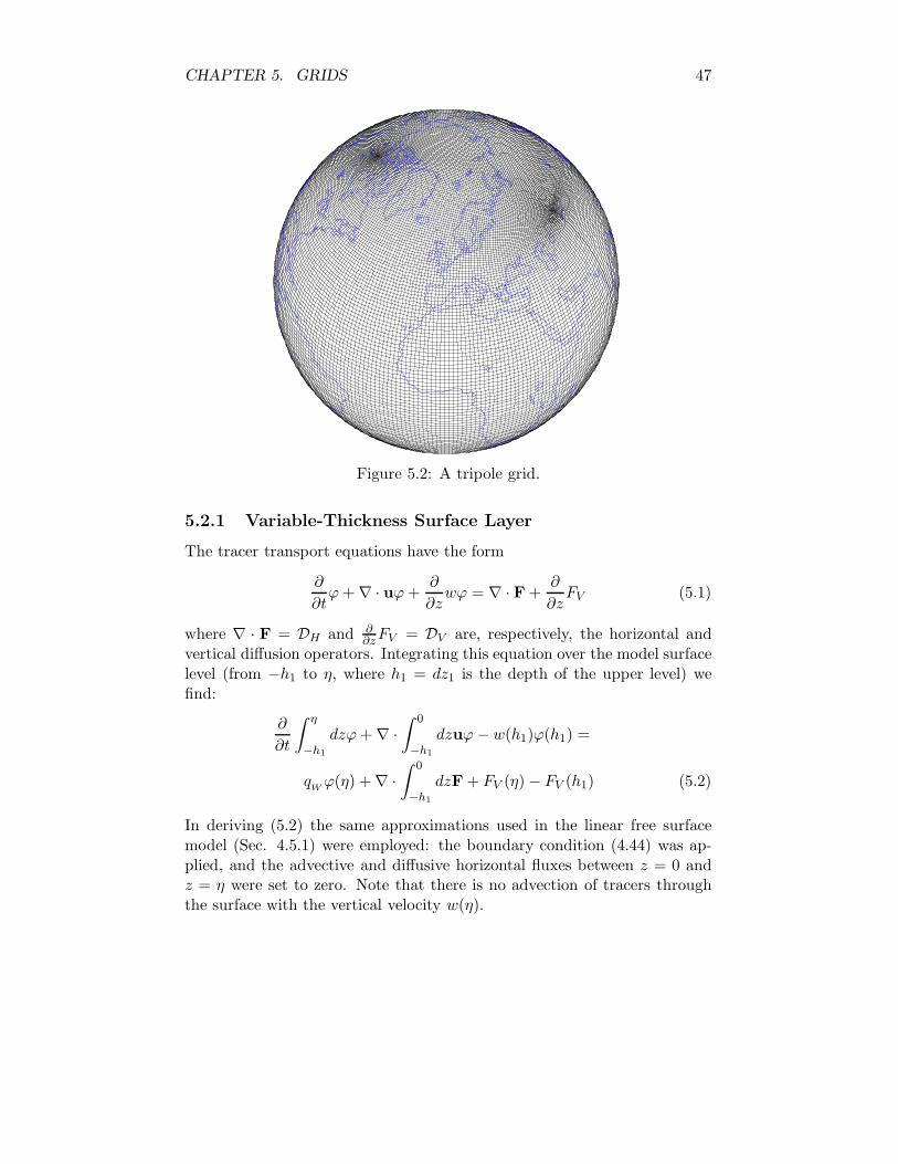
CHAPTER 5. GRIDS 47
Figure 5.2: A tripole grid.
5.2.1 Variable-Thickness Surface Layer
The tracer transport equations have the form
∂
∂tϕ+ ∇ · uϕ+
∂
∂zwϕ = ∇ · F +
∂
∂zFV (5.1)
where ∇ · F = DH and ∂∂zFV = DV are, respectively, the horizontal and
vertical diffusion operators. Integrating this equation over the model surfacelevel (from −h1 to η, where h1 = dz1 is the depth of the upper level) wefind:
∂
∂t
∫ η
−h1
dzϕ+ ∇ ·∫ 0
−h1
dzuϕ − w(h1)ϕ(h1) =
qWϕ(η) + ∇ ·
∫ 0
−h1
dzF + FV (η) − FV (h1) (5.2)
In deriving (5.2) the same approximations used in the linear free surfacemodel (Sec. 4.5.1) were employed: the boundary condition (4.44) was ap-plied, and the advective and diffusive horizontal fluxes between z = 0 andz = η were set to zero. Note that there is no advection of tracers throughthe surface with the vertical velocity w(η).
CHAPTER 5. GRIDS 48
Some care must be taken to specify the tracer fluxes through the air-seainterface. The total tracer flux seen by the ocean model at the surface isgiven by
FT = qWϕ(η) + FV (η) , (5.3)
where ϕ(η) is the tracer concentration at the sea surface and qWϕ(η) repre-
sents the advection of tracers in the ocean relative to the sea surface due tothe freshwater flux. The atmosphere (or sea ice model) sees a flux of tracersinto the ocean given by
QT = qWϕ
W+Qϕ , (5.4)
where ϕW
is the tracer concentration in the freshwater being added or re-moved from the ocean, (for simplicity we assume here that locally there willbe only one source of freshwater, and omit the sum over different types fresh-water sources – see (3.13)), and Qϕ is any additional flux of tracers (e.g., fortemperature in the open ocean it corresponds to the sum of sensible, latent,shortwave and longwave heat fluxes). In reality there is a very thin bound-ary layer where the tracer concentration varies continuously and ϕ(η) = ϕ
W
at the interface. The models do not resolve this boundary layer and so ingeneral ϕ(η) 6= ϕ
W. However, the total flux must be conserved across the
boundary layer, so that FT = QT , and this can be used to eliminate ϕ(η) interms of ϕ
W. Substituting (5.4) for (5.3) in (5.2), we obtain
∂
∂t(h1 + η)ϕ + h1∇ · u1ϕ1 − w1ϕ(h1) =
h1∇ · F1 +Qϕ − FV (h1) + qWϕ
W(5.5)
where now the flux Qϕ is applied as the surface boundary condition on DV .The integrals over the surface layer have been evaluated by assuming themodel variables are constant within the surface layer. w1 is the velocityat the bottom of the surface layer and w1ϕ(h1) represents tracer advectionthrough the bottom of the surface layer. Dividing (5.5) by h1, we arrive atthe tracer transport equation (3.11).
It remains to specify the freshwater tracer concentrations ϕW
. In thecase of salinity the default choice in the code is ϕ
W= S
W= 0, that is, the
freshwater flux qW
= P −E+R−Fice+Mice is assumed to have zero salinity(where P , E, R, Fice and Mice are the freshwater fluxes associated withprecipitation, evaporation, river runoff, freezing and melting of sea ice). Inthe case of potential temperature, the default is to assume the freshwater has
CHAPTER 5. GRIDS 49
the same temperature as the model surface layer, so that ϕW
= ΘW
= Θ1.However, in general the tracer concentration in the freshwater may varydepending on its source (precipitation, evaporation, etc.), and the defaultassumption that these are all given by a single value ϕ
Was in (5.4) may
be inadequate. When coupling to atmospheric or sea-ice models a moreaccurate accounting of the fluxes may be needed to ensure they are conservedbetween component models.
Combining (5.5) with the transport equations in the subsurface levelsand integrating over volume, we find
d
dt
∫dV ϕ =
∫da (Qϕ + q
Wϕ
W) . (5.6)
Thus tracers are conserved in the absence of surface fluxes. This is also trueof the time-discretized equations in the model. In particular, if there are nosurface fluxes of salinity, QS = 0, and if the freshwater flux has zero salinity(ϕ
W= S
W= 0), then total salt is conserved.
The time discretization of (5.5) or (3.11) is given by (4.1) for leapfrogsteps and by (4.6) and (4.7) for forward and backward (Matsuno) timesteps.All of these discrete equations conserve global mean tracers exactly in thesense of (5.6).
There is also a small error in the time discretization associated withthe fact that we have adopted a three-time-level leapfrog scheme for thetracer transport equations (4.1), but a two-time-level discretization for thebarotropic continuity equation (4.48). Note that in the limit of a constanttracer ϕ = 1 the continuous transport equation (5.1), in the absence ofsurface forcing, reduces to the continuity equation ∇ · u + ∂w
∂z = 0, andthe vertically integrated transport equations also reduce to the barotropiccontinuity equation (4.46). This does not hold for the discrete equationsbecause of the inconsistency between the two- and three-time-level schemes.The consequence of this is that a tracer which is initially constant in spacemay evolve to have some small spatial variations. However, this error issecond-order in time and is typically extremely small. In a test problem in-volving the Goldsborough-Stommel circulation (Griffies et al., 2001), whichinvolves only freshwater forcing at the surface, the temperature field, whichis initially constant, deviates from its initial value by only 1 part in 107 ina 100-year integration, and furthermore, the error does not accumulate intime. Therefore, we feel that this error is small enough that it will not causeproblems in long-term climate simulations.
Finally, note that the time discretization error when momentum accel-eration is used, see Sec. 4.2.1, may lead to a computational instability when

CHAPTER 5. GRIDS 50
the variable thickness surface layer option is used with explicit fresh waterfluxes. Because of this possibility, we advise using the variable thicknesssurface layer option with virtual salt fluxes if momentum acceleration, withα 6= 1, is being used.
Nullspace Removal
The operator for the implicit solution of the barotropic equations for thesurface height η in (4.52) contains the Laplacian-like term (4.53). On theB-grid this nine-point Laplacian-like operator contains two null eigenvec-tors: a constant field and a global checkerboard (+/− or black/white) field(a checkerboard field has the value of +1 in black cells and −1 in whitecells). The Laplacian operator on the B-grid annihilates both these typesof null fields (i.e., they have zero eigenvalue). On the C-grid, the globalcheckerboard is not a null eigenvector; for this reason all the horizontal dif-fusive operators in POP have an approximate C-grid discretization, allowinggrid-scale checkerboard noise to be damped by these operators. However,the presence of a checkerboard component in the surface height field doesnot significantly affect the dynamical solution in most cases. The dominanteffect of the surface height is through its contribution to the surface pres-sure gradient, and on the B-grid the gradient operator also does not see thecheckerboard field. There is only a small indirect effect on the vertical ve-locities in T-columns because they are determined by vertically integratingthe continuity equation with the surface boundary condition (3.16), whichdepends on η.
In the implicit free surface formulation, the extra term on the left in(4.52) is a diagonal term associated with the free surface (the ∂t η term inthe barotropic continuity equation). Without this diagonal term, as in thecase in the rigid-lid surface pressure formulation (Smith et al., 1992), the nulleigenvectors are not removed by the operator, and can creep into the itera-tive solution. The diagonal term shifts the eigenvalue of both constant andcheckerboard fields away from zero so that they are damped. Therefore, inmost cases it is not necessary to explicitly remove constant or checkerboardfields from the solution of the implicit free-surface system. However, experi-ence has shown that the solution sometimes does develop large but localizedregions where checkerboard noise appears in the surface height. The exactnature of such regional checkerboarding is not completely understood. Itcan even occur in the rigid-lid streamfunction formulation using an approx-imate five-point operator for the barotropic operator which has no globalcheckerboard nullspace. Note that a five-point approximation is allowed in

CHAPTER 5. GRIDS 51
this case but not in the surface pressure or free-surface formulations, becausethe five-point approximation to the nine-point B-grid operator violates en-ergetic consistency (Smith et al., 1992). Experience has also shown thatthis regional checkerboarding does not affect the dynamical solution, againbecause it is almost completely invisible to the gradient operator. However,with the variable-thickness surface layer (Sec. 5.2.1), such regional checker-boarding can appear in the solution and then slowly accumulate over time,eventually leading to large checkerboard components that can affect the so-lution, either by contributing a large roundoff error to the pressure gradient,or by becoming so large that in some cells the surface height descends belowthe bottom of the surface layer.
When complicated lateral boundaries are included in the computationalmesh, other global null eigenvectors besides the constant and checkerboardfields can also exist. These occur when the domain contains quasi-isolatedbays that are only connected to the rest of the ocean through openingsof one or two cell faces. These regions can have their own constant andcheckerboard nullspaces. There are two types of quasi-isolated bays thatneed to be considered: 1) bays that are connected to the rest of the oceanat the surface by only one face of a T-cell, and 2) bays that are connectedby two adjacent faces of the same T-cell, so that the mouth of the bay isacross the diagonal of the T-cell. If either of these types of bay is in thegrid, a checkerboard nullspace component of the solution can accumulate inthe bay. In the first type of bay, a constant nullspace can also accumulate.In these smaller areas, the problems mentioned above (leading to roundofferror or complete emptying of surface cells) accumulate more quickly in time.Normally, bays of the first type do not appear, because it is the usual practiceduring construction of a grid to eliminate all points that are connected tothe open ocean by only one cell face (such points have no influence on theflow except through diffusion across the open face). But when the variable-thickness surface layer is used, it is necessary to remove all isolated baysof both types in order for the model to run stably. Once these bays areeliminated from the grid, it is still necessary to remove the global constantand checkerboard nullspaces associated with the full domain, to preventthem from slowly accumulating over time. The null fields are projectedout of the solution subject to two constraints: 1) the resulting field has nocheckerboard component; and 2) the projection leaves the global mean sealevel unchanged. Denoting the null eigenvectors Pconst and Pcheck, whichare normalized to 1 and ±1, respectively, the nullspaces can be projected outwith the following operation (here X is the surface height field considered
CHAPTER 5. GRIDS 52
as a one-dimensional vector, and X′ is the same field after the projection):
X′ = X + aPconst − bPcheck
a =XcheckVcheck
N Vconst −M Vcheck
b =XcheckVconst
N Vconst −M Vcheck
Xcheck =∑
X · Pcheck ,
N =∑
Pconst · Pconst ,
M =∑
Pcheck ·Pcheck ,
Vcheck =∑
da ·Pcheck ,
Vconst =∑
da ·Pconst , (5.7)
where da is the one-dimensional vector of cell areas, and the sums are overall surface cells. It is straightforward to show that
∑X′ · Pcheck = 0 and∑
X′ · da =∑
X · da. The latter constraint ensures the projection doesnot change the global mean sea level. This projection is applied once eachtimestep immediately after the barotropic equations are solved for η.
5.2.2 Partial Bottom Cells
To better represent the bottom topography, we employ the idea of partialbottom cells introduced by Adcroft et al. (1997) and later developed forthe MOM model by Pacanowski and Gnanadesikan (1998), for which thethickness of bottom cells is allowed to vary in space. When we place traceror pressure points at the center of partial bottom cells, as shown in Fig-ure 5.3, the finite difference for horizontal derivatives between two adjacentpoints introduces an error because these points are located at different ver-tical positions. More specifically, when we compute the horizontal pressuregradient, we have
∂p
∂x
∣∣∣∣z=−h(x)
=∂
∂x
[p |z=−h(x)
]− gρ |z=−h(x) h(x) , (5.8)
where h(x) can be regarded as the position of tracer points. Without thesecond term on the right hand side of (5.8), the pressure gradient does notvanish even for ρ = ρ(z) for which we expect px|z=−h(x) = 0. Even thoughwe include the correction term, px vanishes only when ρ(z) varies linearly
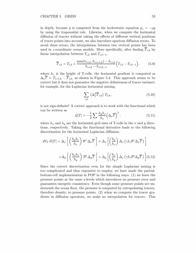
CHAPTER 5. GRIDS 53
in depth, because p is computed from the hydrostatic equation pz = −ρgby using the trapezoidal rule. Likewise, when we compute the horizontaldiffusion of tracers without taking the effects of different vertical positionsof tracer points into account, we also introduce spurious diffusion errors. Toavoid these errors, the interpolation between two vertical points has beenused in z-coordinate ocean models. More specifically, after finding T i,k bylinear interpolation between Ti,k and Ti,k−1,
T i,k = Ti,k +min(hzi,k, hzi+1,k) − hzi,k
hzi,k − hzi,k−1
(Ti,k − Ti,k−1
), (5.9)
where hz is the height of T-cells, the horizontal gradient is computed as∆xT = Ti+1,k − T i,k, as shown in Figure 5.4. This approach seems to becorrect but it does not guarantee the negative definiteness of tracer variance:for example, for the Laplacian horizontal mixing,
∑
i,k
(∆2
xT i,k
)Ti,k , (5.10)
is not sign-definite! A correct approach is to work with the functional whichcan be written as
G[T ] = −1
2
∑ hyhz
hx
(∆xT
)2, (5.11)
where hx and hy are the horizontal grid sizes of T-cells in the x and y direc-tions, respectively. Taking the functional derivative leads to the followingdiscretization for the horizontal Laplacian diffusion:
dVT D[T ] = ∆x
[(hyhz
hx
)κx ∆xT
]+ ∆x
[(hy
hx
)∆z
(γhzκ
x∆xT) ]
+∆y
[(hxhz
hy
)κy ∆yT
]+ ∆y
[(hx
hy
)∆z
(γhzκ
y∆yT) ]
.(5.12)
Since the correct discretization even for the simple Laplacian mixing istoo complicated and thus expensive to employ, we have made the partial-bottom-cell implementation in POP in the following ways: (1) we leave thepressure points at the same z-levels which introduces no pressure error andguarantees energetic consistency. Even though some pressure points are un-derneath the ocean floor, the pressure is computed by extrapolating tracers,therefore density, to pressure points. (2) when we compute the tracer gra-dients in diffusion operators, we make no interpolation for tracers. This
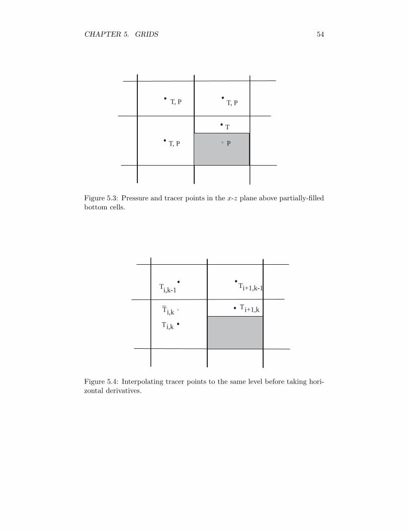
CHAPTER 5. GRIDS 54
T, P
T
P
T, P T, P
Figure 5.3: Pressure and tracer points in the x-z plane above partially-filledbottom cells.
T
TT_
i,k
i,k i+1,k
i,k-1T Ti+1,k-1
Figure 5.4: Interpolating tracer points to the same level before taking hori-zontal derivatives.
CHAPTER 5. GRIDS 55
approach introduces spurious diffusion errors but guarantees at least thesign-definite tracer variances, which has been given up in other OGCMs.Our test results show the error introduced by the second approach is sosmall that we can avoid any complication involving the interpolation.
Discretization
After reading the height of bottom T-cells, POP uses two additional three-dimensional arrays for the thickness of T-cells, DZTi,j,k, and the thicknessof U -cells defined as
DZUi,j,k = min(DZTi,j,k,DZTi+1,j,k,DZTi,j+1,k,DZTi+1,j+1,k). (5.13)
Due to these variable cell heights, the spatial discretizations described inSec. 3 need to be modified as shown in the following.
Tracer Advection:
LT (ϕ) =1
HT ∆Ty
δx
(HU∆U
y uxyϕx)
+1
HT ∆Tx
δy
(HU∆U
x uyxϕy)
+ δz (wϕz) , (5.14)
where ∆(U,T )x = DX(U,T), ∆
(U,T )y = DY(U,T), H(U,T ) = DZ(U,T), and the
vertical velocity w at bottom T -cells is found as
wk+1 − wk =1
∆Ty
δx
(∆U
y HUux
y)
+1
∆Tx
δy
(∆U
xHUuy
x). (5.15)
Laplacian Horizontal Tracer Diffusion:
DH(ϕ) =1
HT ∆Ty
δx(AH
x∆y∆
izδxϕ
)+
1
HT ∆Tx
δy(AH
y∆x∆j
zδyϕ), (5.16)
where ∆x=HTN, ∆y=HTE, and
∆iz = min(DZTi,j,k,DZTi+1,j,k), ∆j
z = min(DZTi,j,k,DZTi,j+1,k). (5.17)
Vertical Tracer Diffusion:
DV (ϕ) =1
HT
[κk+ 1
2
(ϕk+1 − ϕk)
(HTk+1 +HT
k)/2−κk− 1
2
(ϕk − ϕk−1)
(HTk +HT
k−1)/2
]. (5.18)

CHAPTER 5. GRIDS 56
Momentum Advection:
LU (α) =1
HU∆Uy
δx
(HU∆U
y uxyxy
αx)
+1
HU∆Ux
δy
(HU∆U
x uyxxy
αy)
+ δz (wαz) . (5.19)
Laplacian Horizontal Friction:
DH(u) =1
HU∆Uy
δx(AM
x∆i
y∆izδxu
)+
1
HU∆Ux
δy(AM
y∆j
x∆jzδyu
)
− AM
HU∆Ux ∆U
y
[∆i
y(HU − ∆i
z)
∆x
x
+∆j
x(HU − ∆iz)
∆y
y]u, (5.20)
where ∆x=HTN, ∆y=HTE, ∆jx=HUS, ∆i
y=HUW, and
∆iz = min(DZUi,j,k,DZUi+1,j,k), ∆j
z = min(DZUi,j,k,DZUi,j+1,k). (5.21)
The last term of (5.20) is the drag due to the no-slip boundary condition atlateral boundaries. Metric terms in the momentum advection and horizontalfriction remain unaffected by partial bottom cells.
Vertical Friction:
DV (u) =1
HU
[κk+ 1
2
(uk+1 − uk)
(HUk+1 +HU
k )/2−κk− 1
2
(uk − uk−1)
(HUk +HU
k−1)/2
]. (5.22)
Hydrostatic Pressure: Since we leave the pressure points at the middle offull cells, the hydrostatic pressure is computed in the same way as for thefull-cell case.
Biharmonic Horizontal Diffusion and Friction: The same operations forthe Laplacian diffusion and friction given by (5.16) and (5.20) for ϕ and u,respectively, are applied twice.

CHAPTER 5. GRIDS 57
Isopycnal Diffusion:
DH(ϕ) =1
HT ∆Ty
δx
[∆y
(HTκzx
δxϕ−HTκSxδzϕzx)]
(5.23)
− 1
∆Tx ∆T
y
δz
[1
HTz
(HT ∆j
x∆yκSxδxϕxz
−HT ∆jx∆yκS2
x
xz
δzϕ
)]
+1
HT ∆Tx
δy
[∆x
(HTκzy
δyϕ−HTκSyδzϕzy)]
− 1
∆Tx ∆T
y
δz
[1
HTz
(HT ∆x∆i
yκSyδyϕyz
−HT ∆x∆iyκS
2y
yzδzϕ)],
where ∆x=HTN, ∆y=HTE, ∆jx=HUS, ∆i
y=HUW, Sx = δxρ/δzρ, and Sy =δyρ/δzρ. In (5.23), for example, in the (x, z)-plane, κ in the two quartercells in either the east or west direction of T-cells right next to any partialcell is reduced to
κei,j,k =
HTi+1,j,k
dzkκi,j,k, κw
i,j,k =HT
i−1,j,k
dzkκi,j,k , (5.24)
where dzk is the full-cell height. Similar reductions are made for κ in the(y, z)-plane, too. Also κ in the lower half of T-cells right above any partialcells and κ in the upper half of any partial cells are modified to
κbottomi,j,k−1 =
HTi,j,k
dzkκi,j,k−1, κtop
i,j,k =HT
i,j,k
dzkκi,j,k . (5.25)
Remember that κ at the lower half of bottom T-cells is set to zero.
Anisotropic Viscosity:
DxH(u) =
1
∆Uy
δx(∆yγσ11x) +
1
∆Ux
δy(∆xγσ12y)
− ∆xk1∆yγσ22xx
+ ∆yk2∆xγσ12yy, (5.26)
DyH(u) =
1
∆Ux
δy(∆xγσ22y) +
1
∆Uy
δx(∆yγσ12x)
− ∆yk2∆xγσ11yy
+ ∆xk1∆yγσ12xx, (5.27)
where ∆x=HTN, ∆y=HTE, γ = 1 at four quarter cells at the centered U-cell and γ’s are defined in two quarter cells adjacent to the U-cell in the

CHAPTER 5. GRIDS 58
east, west, north and south directions as
γe =min(HU
i,j,k,HUi+1,j,k)
HUi,j,k
,γw =min(HU
i,j,k,HUi−1,j,k)
HUi,j,k
, (5.28)
γn =min(HU
i,j,k,HUi,j+1,k)
HUi,j,k
,γs =min(HU
i,j,k,HUi,j−1,k)
HUi,j,k
. (5.29)
Due to no-slip boundary conditions imposed at lateral boundaries, the ve-locity gradients to compute the stress tensor σ are re-defined as
(δxu)e =
1
∆x(γeui+1,j,k − ui,j,k) ,(δxu)
w =1
∆x(ui,j,k − γwui−1,j,k) , (5.30)
(δxu)n =
1
∆y(γnui,j+1,k − ui,j,k) ,(δxu)
s =1
∆y(ui,j,k − γsui,j−1,k) , (5.31)
(k1u)e = ke1
ui,j,k + γeui+1,j,k
2,(k1u)w = kw
1
ui,j,k + γwui−1,j,k
2, (5.32)
(k2u)n = kn2
ui,j,k + γnui,j+1,k
2,(k2u)s = ks
2
ui,j,k + γsui,j−1,k
2, (5.33)
where ke1, k
w1 , kn
2 and ks2 are the metric terms defined on the east, west,
north and south faces.

Chapter 6
Advection
POP supports a few advection schemes, primarily for tracers where conser-vation and monotonicity requirements are stronger. While basic centeredschemes for tracers and advection are described in Chapter 3, this chapterdescribes other advection schemes implemented in POP.
6.1 Third-Order Upwind Advection
Third-order upwind schemes and variants of this scheme were introducedby Leonard (1979a). Our implementation of third-order upwinding simplyinvolves the substitution of three-point interpolation for the two-point cen-tered average in the determination of the tracer value at cell faces, andremains in leapfrog temporal implementation.
It should be noted that improved temporal implementations have beenexplored in Farrow and Stevens (1995), where they apply a predictor-cor-rector sequence, and in Holland et al. (1998), where in addition to docu-menting our implementation they also describe a reorganization of termsinto two groups, one of which is entirely centered in space, the other havinga dissipative form.
The finite-difference expression for the advection of tracers is
ADV (i, j, k) = − (uE T ∗E − uW T ∗
W )/DXT
− (vN T ∗N − vS T ∗
S)/DYT
− (wk T∗T − wk+1 T
∗B)/dz (6.1)
where uW , uE , vS , vN are the T-grid cell face centered velocity components
59

CHAPTER 6. ADVECTION 60
and the directions W,E,S and N are with respect to the logical coordinates.
uE(i) = (ui,jDYUi,j + ui,j−1DYUi,j−1)/(2DXTi,j)
uW (i) = uE(i− 1)
vN (j) = (vi,jDXUi,j + vi−1,jDXUi−1,j)/(2DXTi,j)
vS(j) = (vi,j−1DXUi,j + vi−1,j−1DXUi−1,j)/(2DXTi,j) (6.2)
and the T ∗ quantities are the cell face centered tracer concentration at theeast, west, north, south, top, and bottom faces. In the standard second-order scheme of POP, these are taken as the arithmetic average of the tracerconcentrations in adjacent cells, e.g.,
T ∗E =
1
2(Ti+1,j + Ti,j) (6.3)
The third point included in the three-point interpolation is taken to bein the upwind direction,
T ∗E(i) =
γTi−1 + β+Ti + α+Ti+1 uE > 0
β−Ti + α−Ti+1 + δTi+2 uE < 0(6.4)
T ∗W (i) = T ∗
E(i− 1) (6.5)
where the coefficients α, β, γ, δ are given by
α+ =dxi(2dxi + dxi−1)
(dxi + dxi+1)(dxi+1 + dxi−1 + 2dxi)
α− =dxi(2dxi+1 + dxi+2)
(dxi + dxi+1)(dxi+1 + dxi+2)
β+ =dxi+1(2dxi + dxi−1)
(dxi + dxi+1)(dxi + dxi−1)
β− =dxi+1(2dxi+1 + dxi+2)
(dxi + dxi+1)(dxi + dxi+2 + 2dxi+1)
γ =−dxidxi+1
(dxi + dxi−1)(dxi+1 + dxi−1 + 2dxi)
δ =−dxidxi+1
(dxi+1 + dxi+2)(dxi + dxi+2 + 2dxi+1)(6.6)
where dx = DXT and the j-index is suppressed for clarity. The interfacetracer values T ∗
N , T∗S , T
∗T , and T ∗
B are obtained in an analogous manner.

CHAPTER 6. ADVECTION 61
6.2 Flux-Limited Lax-Wendroff Algorithm
A flux-limited version of the second-order Lax-Wendroff advection schemehas been introduced into POP. The scheme is designed to reduce, but notcompletely eliminate, the production and amplification of artificial extrema.The artificial extrema are not completely eliminated because the flux limiteris not a true multidimensional limiter. The scheme is constructed by com-bining a one-dimensional flux-limited scheme with a dimensional splittingtechnique. We describe in order: time stepping, the non-flux limited versionof the one dimensional scheme, the flux limiter, the dimensional splittingtechnique, and how boundary conditions are handled.
The advection schemes currently available in POP, centered and third-order upwind, use leap-frog time stepping. That is, when computing thetracer tendency between time levels n− 1 and n+ 1 the advective operatorLT is applied to the tracer φ at time level n. However, flux-limited advectionschemes are generally designed for forward-in-time time stepping. So thisscheme applies the advective operator to the tracer φ time level n− 1. Notethat velocities are still from time level n and thus are time-centered.
The advection equation in one dimension, in advective form, is
φt + uφx = 0, (6.7)
where u is the component of the velocity in the dimension under considera-tion. We rewrite (6.7) as
φt + (uφ)x = uxφ. (6.8)
While we assume that ∇ · ~U = 0, we do not assume the velocity to bedivergence-free in one dimension. Because of this, (6.7) and (6.8) do notnecessarily conserve total tracer content. Conservation of total tracer con-tent will later be recovered with the splitting scheme described below.
For our description of the non-flux limited one-dimensional scheme, wetemporarily change notation from that used elsewhere in this manual. Weconsider a one dimensional grid where the jth interval of the grid is denotedIj . Its width is ∆xj, its midpoint is xj , and its left and right endpointsare xj−1/2 and xj+1/2 respectively. Thus, we have ∆xj = xj+1/2 − xj−1/2.Additionally, we define ∆xj+1/2 ≡ (∆xj + ∆xj+1) /2 = xj+1 − xj. Theadvection scheme under consideration discretizes (6.8) as
φn+1j = φn−1
j − 2∆t
∆xj
(Fj+1/2 − Fj−1/2
)+
2∆t
∆xj
(uj+1/2 − uj−1/2
)φn−1
j , (6.9)
CHAPTER 6. ADVECTION 62
where super- and sub-scripts indicate time and space indices respectivelyand ∆t is the time step. Fj+1/2, the advective flux of φ through xj+1/2, isgiven by
Fj+1/2 ≡ uj+1/2φj+1/2,
where φj+1/2 is an approximation to the average value of φ at xj+1/2 overtn−1 ≤ t ≤ tn+1. Since φj+1/2 does not represent φ at a particular timelevel, we do not denote a time level in a superscript. φj+1/2 is constructedby
1. approximating φ(x, tn−1
)with a linear fit p(x),
2. advecting p(x) exactly with velocity uj+1/2,
3. taking φj+1/2 to be the average value of the advected p(x) at xj+1/2
over tn−1 ≤ t ≤ tn+1.
The linear fit p(x) is constructed by equating p(x)’s average values overintervals Ij+k near xj+1/2 to φn−1
j+k for k ∈ 0, 1. That is, p(x) satisfies theconstraints
1
∆xj+k
∫
Ij+k
p(x) dx = φn−1j+k . (6.10)
When the constructed p(x) is advected and averaged at x = xj+1/2 overtn−1 ≤ t ≤ tn+1, the result is
φj+1/2 = φn−1j +
1
2
(∆xj − 2uj+1/2∆t
) φn−1j+1 − φn−1
j
∆xj+1/2(6.11)
= φn−1j+1 − 1
2
(∆xj+1 + 2uj+1/2∆t
) φn−1j+1 − φn−1
j
∆xj+1/2. (6.12)
This is the familiar Lax-Wendroff scheme in a form that is appropriate fora stretched grid. We present the different forms of the same expression inanticipation of the application of flux limiters.
The above description assumes that the velocity is specified at intervalboundaries. This leads to a natural implementation in the multidimensionalsetting when normal velocities are specified at midpoints of tracer cell faces,as is done with Arakawa C-grids (Arakawa and Lamb, 1977). However,POP utilizes an Arakawa B-grid, where velocities are specified at tracercell corners. Since the one-dimensional scheme use the face velocity for thetracer face value construction, e.g. (6.11), it is necessary to compute a face

CHAPTER 6. ADVECTION 63
velocity from the B-grid corner velocities. The normal velocity for the eastface of the i, j tracer cell is computed as
Ueasti,j = 0.5 (DYUi,jUi,j + DYUi,j−1Ui,j−1) /HTEi,j , (6.13)
where DYUi,j = (HTEi,j + HTEi,j+1) /2, HTEi,j is the length of the eastface, and Ui,j and Ui,j−1 are the zonal velocities at the north-east and south-east corners respectively. We note that (6.13) requires adjustment if POP isconfigured with partial bottom cells and that a formula analogous to (6.13)holds for Vnorth
i,j .In one dimension, we employ a flux limiter that is based on the work
of Hundsdorfer and Trompert (1994), noting that the flux limiter presentedthere is in fact equivalent to the ULTIMATE flux limiter of Leonard (1979b).Solutions of (6.7) are constant along characteristics, which implies that localextrema are not created or amplified. The purpose of the flux limiter is toconstrain the discretization to have this property as well. This is done bymodifying, as necessary, the advective flux Fj+1/2. In order to simplify thepresentation, we initially assume u > 0. We write Fj+1/2 as
Fj+1/2 = uj+1/2φj+1/2
= uj+1/2
(φn−1
j + ψj+1/2
(φn−1
j+1 − φn−1j
)), (6.14)
where ψj+1/2 is to be determined. A priori, we will impose 0 ≤ ψj+1/2 ≤ 1 inorder to avoid extrapolation in the construction of φj+1/2. We seek furtherconstraints on ψj+1/2 that will ensure
min(φn−1
j−1 , φn−1j
)≤ φn+1
j ≤ max(φn−1
j−1 , φn−1j
). (6.15)
Note that constraints on ψj+1/2 are ensuring extrema constraints on theinterval that is upwind of xj+1/2 and that these extrema constraints areexpressed in terms of upwind values. Given this form for Fj+1/2, (6.9)becomes
φn+1j = φn−1
j − 2∆t
∆xj
[uj−1/2φ
n−1j + uj+1/2ψj+1/2
(φn−1
j+1 − φn−1j
)
− uj−1/2φn−1j−1 − uj−1/2ψj−1/2
(φn−1
j − φn−1j−1
) ]
(6.16)
We now consider two very specific cases and then the more general thirdcase:
CHAPTER 6. ADVECTION 64
Case I : φn−1j = φn−1
j−1
In this case, (6.16) reduces to
φn+1j = φn−1
j −2uj+1/2∆t
∆xjψj+1/2
(φn−1
j+1 − φn−1j
),
and (6.15) reduces to φn+1j = φn−1
j . Together, these imply ψj+1/2 = 0.
Case II : φn−1j = φn−1
j+1
In this case, (6.16) reduces to
φn+1j = φn−1
j −2uj−1/2∆t
∆xj
(1 − ψj−1/2
) (φn−1
j − φn−1j−1
),
so there is no constraint on ψj+1/2.
Case III :(φn−1
j+1 − φn−1j
)(φn−1
j − φn−1j−1
)6= 0
Letting θj =(φn−1
j − φn−1j−1
)/(φn−1
j+1 − φn−1j
), (6.16) becomes
φn+1j =
[1 − 2∆t
∆xj
(uj−1/2
(1 − ψj−1/2
)+ uj+1/2ψj+1/2/θj
) ]φn−1
j
+2∆t
∆xj
(uj−1/2
(1 − ψj−1/2
)+ uj+1/2ψj+1/2/θj
)φn−1
j−1 .
This expresses φn+1j as a linear combination of φn−1
j and φn−1j−1 where the
weights sum to 1. Given such a representation, (6.15) is equivalent to re-quiring the weights to be between 0 and 1. Thus, (6.15) is equivalent to
0 ≤ 2∆t
∆xj
(uj−1/2
(1 − ψj−1/2
)+ uj+1/2ψj+1/2/θj
)≤ 1,
which in turn is equivalent to
0 ≤uj−1/2
uj+1/2
(1 − ψj−1/2
)+ ψj+1/2/θj ≤
∆xj
2uj+1/2∆t, (6.17)
where we have used the assumption uj+1/2 > 0. We now suppose that
ψj+1/2 = max(0,min
(1, ψ0
j+1/2, µjθj
)), (6.18)
CHAPTER 6. ADVECTION 65
where µj ≥ 0 is to be determined, and ψ0j+1/2 is the value of ψj+1/2 that
corresponds to the non-flux limited advection scheme. Then
0 ≤ ψj+1/2 ≤ 1 and 0 ≤ ψj+1/2/θj ≤ µj .
It follows that
0 ≤uj−1/2
uj+1/2
(1 − ψj−1/2
)+ ψj+1/2/θj ≤
uj−1/2
uj+1/2+ µj.
Comparing this to (6.17), we see that (6.17), and thus (6.15), will be ensuredif
µj ≤∆xj
2uj+1/2∆t−uj−1/2
uj+1/2=
∆xj − 2uj−1/2∆t
2uj+1/2∆t.
In the above presentation we assumed that u > 0. The velocities usedin the analysis were uj+1/2 and the velocity in the upwind direction, uj−1/2.With this in mind, the remaining cases to consider are u < 0, uj+1/2 > 0and uj−1/2 < 0, and uj+1/2 < 0 and uj+3/2 > 0. The last velocity signpair is merely a shift by +1 of the j indices from the second pair, so it isnot necessary to separately consider this case. We note that the convergingvelocity pair uj+1/2 < 0 and uj−1/2 > 0 does not arise in our analysis becausewhen uj+1/2 < 0, the analysis depends on uj+3/2.
We now consider the case where u < 0. In order to maintain the no-tion that smaller values of ψj+1/2 correspond to greater diffusion, (6.14) isreplaced with
Fj+1/2 = uj+1/2φj+1/2 = uj+1/2
(φn−1
j+1 − ψj+1/2
(φn−1
j+1 − φn−1j
)). (6.19)
In order to maintain the notion that constraints on ψj+1/2 are ensuringextrema constraints on the upwind interval, (6.15) is replaced with
min(φn−1
j+2 , φn−1j+1
)≤ φn+1
j+1 ≤ max(φn−1
j+2 , φn−1j+1
). (6.20)
Assuming ψj+1/2 = max(0,min
(1, ψ0
j+1/2, µj+1/θj+1
)), we find, with sim-
ilar algebra, that (6.20) will be satisfied if
µj+1 ≤∆xj+1 + 2uj+3/2∆t
−2uj+1/2∆t.
We finally consider the case where uj+1/2 > 0 and uj−1/2 < 0. In this case,we use (6.14) for Fj+1/2 and (6.19) for Fj−1/2. Then (6.9) becomes
φn+1j = φn−1
j − 2∆t
∆xj
[uj+1/2ψj+1/2
(φn−1
j+1 − φn−1j
)
+ uj−1/2ψj−1/2
(φn−1
j − φn−1j−1
) ].
CHAPTER 6. ADVECTION 66
Since xj is upwind of both xj+1/2 and xj−1/2, we use constraints on both
ψj+1/2 and ψj−1/2 to ensure extrema constraints on φn+1j . Since there are
no points upwind of xj, the extrema constraints reduce to φn+1j = φn−1
j .This can only be satisfied if
0 = uj+1/2ψj+1/2
(φn−1
j+1 − φn−1j
)+ uj−1/2ψj−1/2
(φn−1
j − φn−1j−1
)(6.21)
We now consider two very specific cases and then the more general thirdcase:
Case I : φn−1j = φn−1
j−1
Then we must have ψj+1/2 = 0. The value of ψj−1 is irrelevant.
Case II : φn−1j+1 = φn−1
j
Then we must have ψj−1/2 = 0. The value of ψj+1 is irrelevant.
Case III :(φn−1
j+1 − φn−1j
)(φn−1
j − φn−1j−1
)6= 0
Then (6.21) can be divided by(φn−1
j+1 − φn−1j
)to obtain
0 = uj+1/2ψj+1/2 + uj−1/2ψj−1/2θj. (6.22)
If θj < 0, the only solution that satisfies 0 ≤ ψ ≤ 1 is ψj+1/2 = ψj−1/2 = 0. Ifθj > 0, we choose the largest values of ψj−1/2 and ψj+1/2 that satisfy (6.22),
ψj−1/2 ≤ max(0,min
(1, ψ0
j−1/2
)), and ψj+1/2 ≤ max
(0,min
(1, ψ0
j+1/2
)).
We do this by setting
ψ∗j+1/2 = max
(0,min
(1, ψ0
j+1/2
)),
ψj−1/2 = max(0,min
(1, ψ0
j−1/2,−uj+1/2/uj−1/2 · ψ∗j+1/2/θj
)),
ψj+1/2 = −uj−1/2/uj+1/2 · ψj−1/2θj.
The dimensional splitting technique follows the technique described insection 2.17.4 of Adcroft et al. (2005). In our implementation of this tech-nique, (6.9) and (6.14) are applied sequentially in the z, x, and y directions.Each application of this pair of equations uses the results from the previousapplication, except for the last term of (6.9), where we use φn−1 in eachiteration. Using φn−1 for this term in each iteration leads to conservationof total tracer content, assuming as we do that the velocity field is diver-gence free. Our choice of the ordering of dimensions is based on simplifying

CHAPTER 6. ADVECTION 67
the implementation. We tested alternating the dimension order in simula-tions of the Stommel gyre test problem of Hecht et al. (1995) and did notfind a meaningful benefit, so we do not vary the dimension order in thethree-dimensional setting.
The flux limiter extends the discrete domain of dependence of Lax-Wendroff in the upstream direction, potentially beyond lateral boundaries.For example, consider the situation where we are computing the ’zonal’ fluxat xj+1/2, uj+1/2 > 0, and there is a solid boundary at xj−1/2. Using (6.14)for Fj+1/2 and uj−1/2 = Fj−1/2 = 0 in (6.9) yields
φn+1j = φn−1
j − 2∆t
∆xjψj+1/2uj+1/2
(φn−1
j+1 − φn−1j
).
Since xj is upwind of xj+1/2, we use constraints on ψj+1/2 to ensure extrema
constraints on φn+1j . Since there are no points upwind of xj in the direction
under consideration, the extrema constraints reduce to φn+1j = φn−1
j . Thiscan only be satisfied if ψj+1/2 = 0. Examining (6.18), this can be achieved by
using θj = 0, which is equivalent to using a fictitious φn−1j−1 = φn−1
j . In otherwords, we use a zero Neumann boundary condition at no-flow boundaries.
Chapter 7
Sub-grid Scale MixingParameterizations
7.1 Horizontal Tracer Diffusion
7.1.1 Laplacian Horizontal Diffusivity
The spatial discretization of the standard Laplacian horizontal tracer diffu-sion with a spatially varying tracer diffusivity A
His described in Sec. 3.3.2.
7.1.2 Biharmonic Horizontal Diffusivity
Biharmonic horizontal tracer diffusion is implemented by applying the La-placian operator (3.18) twice. Specifically,
D(4)H (ϕ) = D(2)
H (A(4)H D(2)
H (ϕ)) (7.1)
where the superscripts (4) and (2) refer to biharmonic and harmonic (Lapla-
cian) operators, and D(2)H is given by (3.18) with AH = 1. A
(4)H is the bihar-
monic diffusivity, which may be spatially varying, and should be negative forpositive-definite diffusion. Here the biharmonic diffusivity is sandwiched be-tween the two applications of the Laplacian operator. An alternate approach(not implemented in the code), following Griffies and Hallberg (2000), is to
include the square-root of −AH inside the second derivative of each D(2)H
operator.
68

CHAPTER 7. SUBGRID MIXING PARAMETERIZATIONS 69
7.1.3 The Gent-McWilliams Parameterization
The transport equation of tracer ϕ is given by
∂
∂tϕ+ (u + u∗) · ∇ϕ+ (w + w∗)
∂
∂zϕ = R(ϕ) + DV (ϕ), (7.2)
where the bolus velocity induced by mesoscale eddies is parameterized, fromGent and McWilliams (1990), as
u∗ =
(ν∇ρρz
)
z
, w∗ = −∇ ·(ν∇ρρz
), (7.3)
where ν is a thickness diffusivity and subscripts x, y, z on ρ and tracers ϕdenote partial derivatives with respect to those variables (this conventionwill be followed below). The Redi isoneutral diffusion operator (Redi, 1982)for small slope can be written as
R(ϕ) = ∇3 · (K · ∇3ϕ), (7.4)
where the subscript 3 indicates the three-dimensional gradient or divergence,i.e., ∇3 = (∇, ∂
∂z ). The symmetric tensor K is defined as
K = κI
1 0 −ρx/ρz
0 1 −ρy/ρz
−ρx/ρz −ρy/ρz |∇ρ|2/ρ2z
, (7.5)
This tensor describes along-isopycnal diffusion that is isotropic in the twohorizontal dimensions. The general anisotropic form of (7.5) is given inSmith (1999). The isopycnal diffusivity κI is in general a function of spaceand time, and a parameterization for variable κI will be described at theend of this section. In POP, we write the bolus velocity in the skew-fluxform (Griffies, 1998):
u∗3 · ∇3ϕ = ∇3 · (u∗
3ϕ) = −∇3 · (B · ∇3ϕ), (7.6)
where we have used ∇3 ·u∗3 = 0. The subscript 3 on the velocity indicates the
three-dimensional velocity, i.e., u∗3 = (u∗, w∗). The antisymmetric tensor B
is given by
B = ν
0 0 ρx/ρz
0 0 ρy/ρz
−ρx/ρz −ρy/ρz 0
. (7.7)
CHAPTER 7. SUBGRID MIXING PARAMETERIZATIONS 70
By substituting (7.7), the transport equation (7.2) can be written
∂
∂tϕ+u·∇ϕ+w
∂
∂zϕ = R(ϕ)+DV (ϕ), R(ϕ) = ∇3 ·(K + B)·∇3ϕ. (7.8)
With a nonlinear equation of state, the isopycnal slopes (Lx, Ly) =(−ρx/ρz,−ρy/ρz) that appear in (7.5) and (7.7) should be replaced withslopes along the local neutral surfaces (McDougall, 1987), which are givenby:
Lx = −αpΘx − βpSx
αpΘz − βpSz(7.9)
with a similar definition for Ly. Here αp = −∂ ρp/∂Θ and βp = ∂ ρp/∂S,where Θ and S are the model potential temperature and salinity, and ρp isthe potential density referenced to the local pressure (or depth).
Discretization of the Diffusion Operator
The functional formalism for deriving positive-definite diffusive operatorsin ocean models was originally used to implement the Gent-McWilliamsparameterization in POP. Later, a collaboration between GFDL and LANLled to an improved implementation that is described in Griffies et al. (1998).The main change in the new formulation is to discretize the neutral slopes(7.9) in a particular way that avoids exciting a nonlinear instability.
The discrete functional formalism is based on the property of the con-tinuous dissipation operator (7.8) that it can be expressed as the functionalderivative of the integral of a positive-definite functional G:
G[ϕ] =1
2
∫dV (∇3ϕ) · K · (∇3ϕ)
=1
2
∫dV κI
[(ϕx + Lxϕz)
2 + (ϕy + Lyϕz)2]
(7.10)
R(ϕ) = − δ
δϕG[ϕ] (7.11)
where δ denotes a functional derivative. That is, G is a functional whosederivative with respect to a tracer field at a given point in space yields theisoneutral diffusive operator R at that point. Note that, as a consequenceof the assumption of isotropic diffusion (7.5), the 3-D functional splits intotwo terms which are effectively 2-D, one in the x − z plane and one in they − z plane.
CHAPTER 7. SUBGRID MIXING PARAMETERIZATIONS 71
The procedure for deriving the discrete operator is to first discretize thefunctional and then take its derivatives with respect to the tracer field ata given point on the computational grid; this yields the positive-definitediffusion operator at that point. In order to discretize the functional on thePOP grid, we need to define all the quantities appearing in G within eachcell. Because gradients involve differences across cell faces, it is convenientto subdivide each T-cell into four subcells, as shown in Figure 7.1, whichshows a central T-cell, its four interior subcells, and the eight surroundingsubcells that contribute to the friction operator when the discrete functionalderivative is taken with respect to the tracer value at the central point. Aunique value of the tracer gradients and isoneutral slopes can be assignedto each subcell, and from these the complete discrete functional G can beconstructed and summed over the grid. Associated with each subcell is theset of its three nearest points (known as the “triad” of points associated withthat subcell), namely, the central point of the full cell to which it belongs,and the two nearest points in the horizontal and vertical directions. Forexample, the triad associated with the subcell in Figure 7.1 labeled (o, ne)is the set of points labeled (o), (n), (e). All the derivatives of the tracerfields needed to construct the functional in a given subcell only involve thetracer values at its triad points. For example, the x and z derivatives of
ϕ in the subcell labeled (o, ne), are given by ϕ(o,ne)x = (ϕ(e) − ϕ(o))/hx and
ϕ(o,ne)z = (ϕ(n) − ϕ(o))/hz , where hx and hz are defined in each subcell as
the distances between the central point (o) and the other two triad pointsin the x and z directions, respectively. Similarly, the derivatives in the
subcell labeled (o, nw) are given by ϕ(o,nw)x = (ϕ(o)−ϕ(w))/hx and ϕ
(o,nw)z =
(ϕ(n)−ϕ(o))/hz . The diffusion coefficient is assumed to have a constant valueacross all four subcells within a given full cell, but can vary from full-cell tofull cell.
Using these definitions of the quantities in each subcell appearing in(7.10), it can be written in the discrete form:
G[ϕ] =1
2
∑
ij
4∑
n=1
(κI)ijVijn[(ϕx + Lxϕz)2 + (ϕy + Lyϕz)
2] (7.12)
where subscripts ij run over all full cells, and subscripts n over subcellswithin a given full cell. Vijn = 1
4hxhydz(k) is the subcell volume (where hy
is the full cell width centered at the same point as hx, and note that theheight of each subcell is taken to be half its full-cell height dz(k) .)
The diffusion operator is then given by the derivative of the discrete
CHAPTER 7. SUBGRID MIXING PARAMETERIZATIONS 72
functional with respect to the velocity at a given point (i′, j′):
Ri′j′ = − 1
V Ti′j′
∂
∂ϕi′j′G[ϕ] (7.13)
where V Ti′j′ = AT
i′j′ dz(k) full-cell volume of cell (i, j, k), and ATi′j′ is the full-
cell area. (Note: in the code AT = TAREA, which is not exactly equalto the sum of the four subcell areas given above, however, the difference issmall and is absorbed in an overall normalization factor.) When taking thederivative with respect to ϕ at the central point, only those subcells in thefull functional whose triad points contain the central point will contributeto the derivative, and these are just the 12 subcells shown in Figure 7.1. Itis straightforward to take the derivative in (7.13) in these 12 subcells andassemble the results into a compact form for the diffusion operator. Theresult is:
V Tij Rij(ϕ) = (V/hx)κI(ϕx + Lxϕz)
e − (V/hx)κI(ϕx + Lxϕz)w
+ (V/hz)κI(Lxϕx + L2xϕz)
n − (V/hz)κI(Lxϕx + L2xϕz)
s
+ similar terms with x replaced by y everywhere. (7.14)
Here overbars with superscripts e, w, etc., denote sums over the four subcellssurrounding the east, west, etc., faces of the central full cell. In computingthe slopes Lx and Ly given by (7.9) it is important that the coefficients αp
and βp be evaluated at the pressure corresponding to the level of the centralpoint of the triad in a given subcell (Griffies et al., 1998); this avoids excitingthe nonlinear instability mentioned above. No-flux boundary conditionson the tracers are implemented by setting κI = 0 in all subcells adjacentto lateral and bottom boundaries. There is no way to derive the bolustransport term in (7.8) and (7.7) from a functional like the diffusive term,but the bolus term in (7.8) involves terms proportional to the off-diagonalterms in the diffusion tensor, and these are discretized in the same way.Thus we find for the full skew flux (R(ϕ) in (7.8))
V Tij Rij(ϕ) = (V/hx)[κIϕx + (κI − ν)Lxϕz]
e
− (V/hx)[κIϕx + (κI − ν)Lxϕz]w
+ (V/hz)[(κI + ν)Lxϕx + κIL2xϕz ]
n
− (V/hz)[(κI + ν)Lxϕx + κIL2xϕz)
s
+ similar terms with x replaced by y everywhere. (7.15)

CHAPTER 7. SUBGRID MIXING PARAMETERIZATIONS 73
(o,ne)(o,se)
(o,nw)(o,sw)(s,nw) (s,ne)
(n,sw) (n,se)(w,ne)(w,se) (e,sw)
(e,nw)(o)(n)
(s)
(w) (e)(ne)
(se)(sw)
(nw)
Figure 7.1: The discretization of the x − z part of the isoneutral diffusionfunctional is accomplished by subdividing each T-cell (shown bounded bythick lines) into four subcells. The central tracer point (T-point) is denotedby “(o)” and the surrounding T-points by “(n)”, “(s)”, “(ne)”, etc. (this isfor notation only, points “(n)” and “(s)” are displaced in the vertical direc-tion.) The four subcells surrounding the central point are labeled “(o,ne)”,“(o,nw)”, etc., and the subcells surrounding the T-cell to the east are la-beled “(e,nw)”, etc. Within each subcell a unique value is defined for allquantities (e.g., the gradients and slope factors appearing in (7.10) that areneeded to evaluate the functional. Only the twelve subcells shown contributeto the friction operator at the central point (see text). (Note: this figureshows a case where the fundamental grid is constructed with U-points inthe exact middle of T-cells in a grid with variable horizontal spacing. Morecommonly T-points are located at the exact center of U-cells. This choice ismade during grid generation and is only determined in the code through theinput grid file.) This figure can also be used for constructing the anisotropicdissipation functional (see Sec. 7.2.3) where the central point represents aU-point.
CHAPTER 7. SUBGRID MIXING PARAMETERIZATIONS 74
If the tracer and thickness diffusion coefficients are chosen equal (κI = ν),then the second terms in brackets in the first line of (7.15) vanish and neednot be computed. (Note: in the code, the above formulae are evaluatedusing the slope functions SLX = −(hx/hz)Lx, SLY = −(hy/hz)Ly, and thedifferences ∆xϕ = hxϕx, etc.) Finally, it should be noted that the last termsin (7.15) involving L2
x (and L2y) are separated and treated implicitly, because
the effective viscous coefficient can be large enough to violate explicit CFLconditions (Cox, 1987). These terms can be written
(V/hz)κIL2xϕz
n − (V/hz)κIL2xϕz
s= δz(κ
′δzϕ),
where κ′ = (AT )−1(V/hz)κI(L2x + L2
y)n
(7.16)
and the last line gives κ′ on the top of the T-cell. κ′ is then added to the ver-tical diffusivity κ in (3.19) and the vertical diffusion is solved implicitly. Forthis reason implicit vertical mixing must be used with the Gent-McWilliamsparameterization. One of the design features of the diffusive operator isthat with a linear equation of state it should be zero when applied to ϕ = ρ.This condition is violated when the above term is treated implicitly whilethe remaining terms are treated explicitly, but in practice this leads to avery small error and is ignored.
Two tapering functions are often applied to the GM coefficient ν and theRedi mixing coefficient κI . The first is for physical reasons and reduces theGM coefficient in the upper boundary layer, see Large et al. (1997). Herethe ocean is not nearly adiabatic, and so the GM parameterization does notapply; instead the isopycnals tend to become more vertical because of thestrong vertical mixing in the upper boundary layer. The tapering occurswhere the depth is less than the local isopycnal slope multiplied by the localRossby radius LR defined by LR = |f |/c0 with c0 = 2m/s and LR is boundedby 15 km ≤ LR ≤ 100 km. Two forms for the factor are in the code, withthe second being faster because there is no sine function.tanh option:
f1 =1
2
[1 + sin
(π(min(1,−z/(|L|LR)) − 0.5)
)](7.17)
else:
f1 =1
2+ 2(min(1,−z/(|L|LR)) − 0.5
)×
(1 − |min(1,−z/(|L|LR)) − 0.5|
)(7.18)

CHAPTER 7. SUBGRID MIXING PARAMETERIZATIONS 75
where |L| = (L2x + L2
y)1
2 . The second function ensures numerical stabilitywhen the isopycnals become too steep. There are four options to reduce the
coefficients κI and ν for |L| ≤ S(κI ,ν)M , where the maximum slope allowed
can be different for SκI
M and SνM . The default values are SκI
M = SνM = 0.01.
The first option was described in Danabasoglu and McWilliams (1995) as
f2 =1
2
[1 − tanh(10|L|/S(κI ,ν)
M − 4)]
(7.19)
for |L| > S(κI ,ν)M , κI = ν = 0. The second option is a faster version without
a tanh function:
f2 =1
2
[1 −
(2.5|L|/S(κI ,ν)
M − 1)(
4 − |10|L|/S(κI ,ν)M − 4|
)](7.20)
with f2 = 1 for |L| ≤ 0.2S(κI ,ν)M and f2 = 0 for |L| ≥ 0.6S
(κI ,ν)M .
The third option is the clipping option described in Cox (1987) wherethe slopes are set to the maximum if they are diagnosed as larger. In thiscase, mixing occurs along the maximum allowed slope. This implies somecross isopycnal mixing when the slopes are steep. The default values areSκI
M = SνM = 0.01.
The fourth option is described in Gerdes et al. (1991) and the factor is
f2 = (S(κI ,ν)M /|L|)2 (7.21)
when the slope is larger than the maximum slope. This option and the firsttwo options retain the adiabatic nature of the parameterization. When κI =ν and SκI
M = SνM , the code runs much faster because the terms proportional
to κI − ν disappear. Because CCSM uses the Near Surface Eddy FluxParamaterization described below, no f1 function is needed. For f2, CCSMuses the second option, but the maximum slopes allowed are much largerthan the default values with SκI
M = SνM = 0.3.
Variable GM Diffusivity
Two options for specifying a variable diffusivity are available. The firstfollows Visbeck et al. (1997), where it is assumed that
κI = αL2
E
TE(7.22)
with a typical value of the constant α as 0.13. In (7.22), the barocliniclength scale LE and the Eady time scale TE are defined as
LE = min(c/|f |,
√c/2β
), (7.23)

CHAPTER 7. SUBGRID MIXING PARAMETERIZATIONS 76
1
TE=
max(|f |,√2cβ)√Ri
, (7.24)
Ri = − g
ρ0H
∫ z1
z2
ρz
|uz|2dz, (7.25)
where β is the meridional gradient of the Coriolis parameter and c is thefirst baroclinic wave speed given by c2 = −gH
∫ z1
z2ρz dz/ρ
0, z1 = −50m and
z2 = −1000m. LE is also bounded below by the smaller horizontal side ofeach grid box. In the code, κI is set to be bounded by 3 × 10⁶ ≤ κI ≤2 × 107cm2/s and κI is set to the lower bounding value where the modeldepth is less than −z1.
A second option is meant to parameterize submesoscale eddies. Thisoption varies the thickness, ν, and isopycnal diffusivity, κI , using a simplifiedversion of the closure of Eden and Greatbatch (2008) (note that thicknessdiffusivity and isopycnal diffusivity are here assumed to be identical). Thethickness diffusivity is given by κI = cL2σ, where σ denotes an inverse eddytime scale and c a constant parameter of order one. L denotes an eddylength scale, which is taken as the minimum of the local Rossby radius Lr
and the Rhines scale LRhi. The latter is estimated from model variables as
LRhi = σ/β, where β = ∂yf , while Lr is given by Lr = min[cr/|f |,
√cr/2β
]
where cr denotes the first baroclinic Rossby wave speed, which is calculatedapproximately by cr ≈
∫ 0−hN/πdz, where h denotes the local water depth.
The inverse eddy time scale σ is given by σ = |∇hb|/N , which is, by thethermal wind relation, for mid-latitudes identical to the Eady growth rateσ = |f |Ri−1/2, where Ri = N2/(∂zu
2 + ∂zv2) denotes the local Richardson
number. To prevent a singularity for σ for N → 0 we use σ = |f |(Ri+γ)−1/2
with γ > 0 which acts effectively as an upper limit for σ and consequentlyfor κI . To prevent a singularity for the time scale σ at the equator, f isreplaced by max(|f |,
√2βcr) when computing σ. The default values for the
parameters of the closure are set to γ = 200 and c = 2. More details aboutthe closure can be found in Eden and Greatbatch (2008) and Eden et al.(2009).
Near Surface Eddy Flux Parameterization
We have implemented a simplified version of the near-boundary eddy fluxparameterization of Ferrari et al., (2008, referred to as FMCD08) for thesurface boundary in POP. We refer to this scheme as the Near Surface EddyFlux (NSEF) parameterization. Here, we present a brief summary of its

CHAPTER 7. SUBGRID MIXING PARAMETERIZATIONS 77
implementation in POP and refer to Danabasoglu et al. (2008) for furtherdetails.
As indicated earlier, the Gent and McWilliams (1990, GM90) parame-terization was developed for the quasi-adiabatic interior, and it is not validnear the boundaries. Therefore, the usual practice is to taper the effectsof parameterized eddy fluxes as the surface (or any other boundary) is ap-proached (see equations (7.17) and (7.18)). For example, both κI and ν aretapered to zero when the ocean surface is approached using the f1 taperfunction in addition to the f2 large slope taper function using
κ∗I = f1f2κI and ν∗ = f1f2ν; (7.26)
the asterisk denotes the tapered values of these diffusivities (Large et al.,1997). This near boundary attenuation of the eddy effects is not physicallyconsistent with observational evidence, particularly near the surface wherethe diabatic mesoscale fluxes may dominate the mixing. FMCD08 includesthe effects of these upper-ocean diabatic fluxes and eliminates the ad-hoc,near-surface taper functions.
The NSEF parameterization requires estimation of two vertical lengthscales: the boundary layer depth (BLD) and the transition layer thickness(TLT). The BLD can exhibit rapid fluctuations during which mesoscale ed-dies are unlikely to change. In contrast, the mixed layer depth (MLD) repre-sents a lower-frequency, i.e. time-filtered, envelope of the surface boundarylayer region. In particular, the mixed layer in our simulations records themaximum depth of the boundary layer after sustained deep mixing events,and it can be considered a measure of the deepest penetration of turbulentmixing in the recent past. Therefore, in our present implementation, we usethe MLD instead of the BLD. Following Large et al. (1997), we define theMLD as the shallowest depth where the local, interpolated buoyancy gradi-ent matches the maximum buoyancy gradient between the surface and anydiscrete depth within that water column. One pass of a grid-scale, five-pointspatial filter is applied to the MLD to eliminate any small scale features. Forsimplicity, we choose to apply no filtering in time.
FMCD08 defines the transition layer as the layer containing all isopycnalswithin an averaging area and time interval that are intermittently exposedto strong turbulent mixing. Thus, TLT is defined by the range of isopycnalsthat can be lifted into the boundary layer by subgrid-scale eddy heavingand/or the subgrid-scale (sub-synoptic) variations of the boundary layer.For this purpose, we first calculate a depth D, using the same equation as

CHAPTER 7. SUBGRID MIXING PARAMETERIZATIONS 78
employed in the f1 taper evaluation above, i.e.,
D = LR|L|. (7.27)
Here, LR is the Rossby deformation radius, representing the preferred hor-izontal length scale of the baroclinic eddies, and L is the isopycnal slope.For simplicity, the former is determined from LR = c0/|f |, subject to anadditional restriction of 15 km ≤ LR ≤ 100 km. Here, c0 = 2 ms−1 isa typical value for the first baroclinic wave speed. With this prescription,LR is constant at 100 km equatorwards of 8 latitude and no other equationis used for the equatorial deformation radius. We compute D at each gridpoint in a vertical column below MLD and search for the shallowest depthwhere D does not reach MLD. This is equivalent to finding the depth dwhere,
MLD < d−D (7.28)
is satisfied for the first time. TLT is simply obtained from
TLT = d− MLD. (7.29)
Because we do not impose any maximum slope restrictions in these compu-tations, TLT can become large or even reach the ocean bottom when thecolumn is still very weakly stratified below the mixed layer. Conversely,TLT can vanish if |L| = 0. The sum of MLD and TLT then defines thediabatic layer depth (DLD) over which the upper-ocean eddy fluxes departfrom their interior formulas.
The eddy-induced vector streamfunction can be split into its mixed layer,ΨML, and transition layer, ΨTL, expressions as follows
ΨML =η − z
η + MLDΨo for − MLD ≤ z ≤ η (7.30)
and
ΨTL =
(z + MLD
TLT
)2
Φ +
(η − z
η + MLD
)Ψo (7.31)
for − DLD ≤ z < −MLD,
respectively. The eddy-induced velocity is obtained using ∇ × Ψ. In theabove equations z is the vertical coordinate, positive upward, and η is thedisplacement of the free surface relative to z = 0. The two functions Ψo and

CHAPTER 7. SUBGRID MIXING PARAMETERIZATIONS 79
Φ are chosen such that Ψ and its vertical derivative are continuous acrossthe base of MLD and the base of TLT. These constraints then yield
Ψo =η + MLD
2(η + MLD) + TLT
(2ΨI + TLT ∂zΨI
)(7.32)
and
Φ = − TLT
2(η + MLD) + TLT
(ΨI + (η + DLD)∂zΨI
), (7.33)
where subscript z denotes partial differentiation. In (7.32) and (7.33), ΨI isthe interior eddy-induced streamfunction at the base of the transition layergiven by the GM90 parameterization, i.e., ΨI = ΨGM(z = −DLD) where
ΨGM = −ν z×∇hρ
∂zρ. (7.34)
In (7.34) ρ is the local potential density and ∇h is the horizontal gradientoperator.
In (7.30), Ψo represents the vector streamfunction value at the base ofMLD. We note that ΨML is linear within MLD, going to zero at the oceansurface. This implies constant eddy-induced velocities with no vertical shearwithin MLD. These eddy-induced velocities, however, must develop a shearin the transition layer to match the interior values. For this purpose, (7.31)represents the simplest choice for ΨTL, which is parabolic, or equivalentlylinear in z for the eddy-induced velocities.
In our present implementation we neglect any variations of the free sur-face height in the above equations by setting η = 0, because all the horizontalfluxes between z = 0 and z = η are already neglected in POP due to thelinearization of the barotropic continuity equation. The existing discreteimplementation of the isopycnal transport parameterization readily subdi-vides a vertical grid cell into a top and a bottom half. We naturally takeadvantage of this doubled vertical grid resolution and use the depths of themid-points of the top and bottom halves as reference depths to determineif a particular half is within MLD, TLT, or the interior. We then evaluateseparate ΨI ’s for the appropriate top and bottom halves of the vertical gridcells that straddle the base of the transition layer. These ΨI ’s are also usedto compute ∂zΨI along the transition layer - interior interface.
With ΨI and ∂zΨI now available at z = −DLD, ΨML and ΨTL canbe evaluated using (7.30), (7.31), (7.32), and (7.33). The interior eddy-induced streamfunction values below the base of the transition layer arethen determined from (7.34).

CHAPTER 7. SUBGRID MIXING PARAMETERIZATIONS 80
The mesoscale eddy fluxes still mix tracers along isopycnal surfaces inthe ocean interior as represented by equation (7.4). Within the mixed andtransition layers, the parameterization for diffusive tracer flux (see FMCD08and Danabasoglu et al. (2008)) is given by
F(ϕ) = −c(z) κH∇hϕ − [1 − c(z)] K · ∇ϕ. (7.35)
In (7.35), κH represents the untapered horizontal eddy diffusivity and ∇h isthe horizontal gradient operator. Of course, the rate of mixing within boththe interior and boundary layer remain the same, so κH has the same valueas the interior κI present in K. The vertical function c(z) is defined by
c(z) =
1, for − MLD < z ≤ η
(z + MLD + TLT)/TLT, for − TLT − MLD < z ≤ −MLD.
Note that we drop the vertical component of F(ϕ) within the mixed layer,because it is found to generate negligible flux divergences at resolutions usedin climate models. With the NSEF parameterization, we do not need the f1
taper any longer, i.e.,
κ∗I = f2 κI and ν∗ = f2 ν, (7.36)
In addition, f2 is only applied in the interior below the transition layer.We note that further sensitivity experiments that also use ν∗ = ν in theocean interior, i.e., no f2, lead to numerical instabilities with our presentparameter choices. This is the default option used in CCSM4.
Vertically-varying Isopycnal and Thickness Diffusivity Coefficients
We provide a vertical dependence of the isopycnal and thickness diffusivitycoefficients which vary with the stratification, N2, following Ferreira et al.(2005) and Ferreira and Marshall (2006). The formulation produces diffusiv-ities that are large in the upper ocean and small in the abyss. We regard useof an N2 dependency as a convenient way of introducing a surface intensifi-cation of the diffusivity coefficients. A brief summary of its implementationin POP2 is presented here and further details are given in Danabasoglu andMarshall (2007).
The vertical variation of κI and ν is specified using
κI =
[N2
N2ref
] [κI
]ref, (7.37)

CHAPTER 7. SUBGRID MIXING PARAMETERIZATIONS 81
and
ν =
[N2
N2ref
] [ν]ref, (7.38)
where N is the local buoyancy frequency computed at the vertical level in-terfaces, and
[κI
]ref
and[ν]ref
are the constant reference values of κI and
ν within the surface diabatic layer (SDL). Nref is the reference buoyancyfrequency obtained just below the SDL, provided that N2 > 0 there. Oth-erwise N2
ref is the first stable N2 below the SDL. The ratio N2/N2ref is set
to 1 for all shallower depths, implying no vertical variation of κI and ν,particularly within the SDL. Between the depth at which N2 = N2
ref andthe ocean bottom, we also ensure that
Nmin ≤ N2
N2ref
≤ 1.0, (7.39)
where Nmin(> 0) is a specified lower limit. Equation (7.39) also implies thatin statically unstable regions, i.e. N2 < 0, N2/N2
ref = Nmin. This approachrelies on the enhancement of vertical mixing coefficients to alleviate anylocal static instability.
The specification of the SDL depends on some other parameterizationchoices. The internal model default for the SDL is the first model levelthickness. If the K-Profile Parameterization (Large et al., 1994) is used,then the SDL is set to the diagnosed boundary layer depth. When theNSEF scheme is also specified, the diabatic layer depth (DLD) becomes theSDL. If one uses neither scheme, then the default internal value likely needsto be modified to reflect the bulk mixed layer depth.
The N2/N2ref profiles are evaluated once per day at the beginning of
a day. We avoid any vertical averaging of the profiles to preserve theirextrema. Instead, N2/N2
ref computed at the top face of a grid cell is simplyused for that grid cell. The resulting diffusivities from (7.37) and (7.38)are subject to the usual diffusive numerical stability criterion. In addition,the zero eddy flux boundary condition at the ocean bottom is imposed bysetting the diffusivities to zero in the bottom halves of the grid boxes. Thus,the effective diffusivities for these bottom grid cells are further reduced byone half.
One can choose to use (7.38) only for ν while using a constant κI . How-ever, given that there are no strong arguments for setting κI different fromν, we use (7.37) and (7.38) for both κI and ν with the same reference dif-fusivity values. We note that, at least for the case of constant diffusivities,the theoretical study of Dukowicz and Smith (1997) supports specifying
CHAPTER 7. SUBGRID MIXING PARAMETERIZATIONS 82
equal values. In the standard nominal ×1 and ×3 configurations, we set[κI
]ref
=[ν]ref
= κH = 3000 m2 s−1 and[κI
]ref
=[ν]ref
= κH = 4000
m2 s−1, respectively. The default for Nmin is Nmin = 0.1. Thus, by about2000-m depth, these reference values are reduced to 300 and 400 m2 s−1,respectively. We note that κH is used if the NSEF option is on (default). Inaddition to the NSEF parameterization, this prescription for vertical varia-tions of the diffusivity coefficients is used in CCSM4.
7.1.4 Parameterization of Mixed Layer Eddies
In principle, the effects of all scales smaller than the model grid scale shouldbe parameterized with subgridscale models. Historically, focus has been onthe mesoscale (≈ 100 km, e.g. Gent and McWilliams, 1990) and finescale(≈ 10 m, e.g. Large et al., 1994) parameterizations. However, recent interesthas focused on the submesoscale (≈ 1 km) physics, because of its ubiquitousrestratifying effect on the mixed layer.
Recent realistic simulations (Oschlies, 2002; Capet et al., 2008a,b,c,d),idealized simulations (Haine and Marshall, 1998; Thomas, 2008; Mahadevanet al., 2009), and theory (Thomas and Lee, 2005; Thomas, 2005; Boccalettiet al., 2007; Thomas et al., 2008; Thomas and Ferrari, 2008) have stud-ied and quantified some effects of the submesoscale that may potentiallyaffect the larger scales resolved by climate models. The parameterizationimplemented in POP follows the theory for one important submesoscaleeffect–restratification by mixed layer eddies–proposed by Fox-Kemper et al.(2008b, hereafter FFH). The FFH parameterization is validated against ide-alized submesoscale-resolving simulations (Fox-Kemper and Ferrari, 2008)and has been implemented and documented in a number of global climatemodels (Fox-Kemper et al., 2008a, 2010). These papers have substantiallymore detail than the short presentation herein and the reader is encouragedto seek them out.
Mixed Layer Eddies (MLEs) are the finite-amplitude result of ageostropicbaroclinic instabilities of the density fronts common throughout the oceanmixed layer (Rudnick and Ferrari, 1999; Ferrari and Rudnick, 2000; Hose-good et al., 2006; Boccaletti et al., 2007). The MLE horizontal scale is nearthe deformation radius of this mixed layer, which is O(1 km), so these eddieswill not be routinely resolved in global- or basin-scale simulations for sometime. Nonetheless they do have effects that are important to be includedin coarse-resolution models. The primary effect of these eddies is to extractpotential energy by restratifying the mean density profile of the upper ocean.
The parameterized restratification is carried out by an eddy-induced
CHAPTER 7. SUBGRID MIXING PARAMETERIZATIONS 83
overturning streamfunction (Ψ), which can be thought of as producing aneddy-induced or quasi-Stokes velocity field (u∗ = ∇ × Ψ). Advection bythe eddy-induced velocity provides the eddy fluxes of tracers, including thebuoyancy skew flux (u′b′ = Ψ × ∇b). Buoyancy is the negative densityanomaly rescaled to have units of acceleration b ≡ g(ρ0 − ρ)/ρ0, as appro-priate for a Boussinesq fluid. Overlines are used to represent the fields in acoarse-resolution model, that is, one not resolving the submesoscale eddies.The MLE fluxes are assumed to occur in addition to resolved or otherwiseparameterized fluxes.
The FFH parameterization is given by
Ψ0 = CeH2∇b
z×z
|f | µ(z), (7.40)
µ(z) = max
0,[1 −
(2zH + 1
)2][1 + 5
21
(2zH + 1
)2],
where H is mixed layer depth, f is the Coriolis parameter, and z is theunit vertical vector. The overline with subscript z on ∇bz is understoodto be the depth-average of ∇b over the mixed layer. The efficiency coeffi-cient Ce is approximately 0.06 (Fox-Kemper et al., 2008b). Note that theparameterization is only nonzero within the mixed layer.
An adaptation to (7.40) that is suitable and justified in a global coarse-resolution model (Fox-Kemper et al., 2010) is:
Ψ = Ce∆s
Lf
H2∇bz × z√f2 + τ−2
µ(z). (7.41)
∆s is an appropriate local gridscale of the coarse model, Lf is an estimate ofthe typical local width of mixed layer fronts, and τ is a timescale for mixingmomentum vertically across the mixed layer (≈1-10 days). Hosegood et al.(2006) suggest Lf is close to the mixed layer deformation radius NH/f ,where N is the buoyancy frequency of the mixed layer stratification. Forstability, a lower cutoff is used: Lf = max(NH/|f |, Lf,min) where Lf,min ischosen in the 1 to 5km range. Likewise, if ∆s is very large, an upper limitnear 1 should be imposed. See Fox-Kemper et al. (2010) for details.
Details of Implementation
Coarse Resolution Rescaling: The FFH parameterization (7.40) depends onthe horizontal density gradient. Coarser models have weaker gradients thanfiner, and sparser observations have weaker gradients than denser. The∆s/Lf factor in (7.41) accounts for the expected dependence of horizontal
CHAPTER 7. SUBGRID MIXING PARAMETERIZATIONS 84
density gradients on resolution. The vertical buoyancy flux given by (7.40)scales as
w′b′ ≡ Ψ×∇b ≈ Ψ ×∇bz ∝ H2|∇bz × z|2|f | . (7.42)
One would like the same vertical buoyancy flux regardless of model reso-lution, and the ∆s/Lf factor is a good approximation (Fox-Kemper et al.,2010). Note that the horizontal fluxes are not necessarily accurately rescaledby this method, and the overturning streamfunction may become very large.However, these submesoscale eddies are so small that they generally havenegligible horizontal fluxes, and the mixed layer vertical stratification soweak that the parameterized horizontal fluxes are small even when thestreamfunction is large. These spurious effects are consequences of the res-olution rescaling that should be inconsequential, although the user shouldkeep their spurious nature in mind.
Timestep Limitation: The overturning streamfunction is thus rescaled as∆s/Lf . The eddy-induced velocity will go as u∗ ∝ ∆s/Lf , so the timestepis limited as though the gridscale were Lf instead of ∆s. In practice u∗ isusually smaller than other velocities in the model–consistent with the smallMLE horizontal fluxes. However, it is possible for the FFH parameterizationto require somewhat smaller timesteps in certain conditions on certain grids,especially with fine vertical resolution where w∗ may determine the timestep.
Steps are taken in POP to ameliorate this timestep limitation for smallLf . 1) A minimum value of Lf , Lf,min, is used (usually in the one to fivekm range). 2) min[∆s, 1]/max[Lf , Lf,min] constrains the scaleup in verycoarse resolution models. As one might expect, the high latitudes where|f | is large are more strongly affected by the choice of cutoff. The mixedlayer frontal scale is often obseved to be smaller than 5km. However, thebuoyancy frequency, N , in the mixed layer is highly sensitive to other pa-rameterization choices (e.g. maximum diffusivity of mixing in KPP), thusthis cutoff is required and should be adjusted along with other model pa-rameters. Generally, the cutoff value should be as small as can be safelyintegrated. In test cases, a 1km cutoff in POP allows a ML depth nearly20% shallower in high latitudes than a 5km cutoff.
High-Resolution Usage: The ∆s/Lf scaling automatically handles re-gional variations of eddy scales in a high-resolution model. If Lf is resolvedin some regions – e.g. where the mixed layer is particularly deep after deepconvection – and not in other regions, the scaling adjusts. A just-resolvedfront (where Lf = ∆s) has no scale-up and insufficient resolution to form anyMLEs. A resolved front with MLEs permitted but not resolved (Lf = 4∆s)

CHAPTER 7. SUBGRID MIXING PARAMETERIZATIONS 85
is boosted by the parameterization, and a well resolved feature (Lf = 20∆s)has negligible effects from the parameterization.
Tracers Other than Buoyancy: The rescaling relies on w′b′ ∝ |∇bz × z|2,which is appropriate for the scaling of density fronts of the near-surfaceocean (Capet et al., 2008c). The FFH parameterization is also used forother tracers, and these fronts will lend similar scaling behavior to thosetracers as well. Thus, the rescaling remains appropriate.
Equatorial Regularization: The division by |f | in the scaling for (7.40)for Ψ0 means that this form cannot be used at the equator. Physically,Boccaletti et al. (2007) and Fox-Kemper et al. (2008b) note that MLEsare largely geostrophic and thus do not restratify in the same way as theequator is approached. Under typical midlatitude situations, the growth ofinstabilities rivals the timescales of mixing events and the eddy fluxes areonly intermittently interrupted. However, as Ψ0 grows near the equator,frictional constraints enter. The FFH parameterization (7.40) is thereforeadapted in (7.41) to converge to a friction slumping rate (Ferrari and Young,1997) as the equator is approached. The frictional time constant τ should beon the order of the timescale between mixing events driven by atmosphericsynoptic variability–a few days to a few weeks.
Adjustable Parameters: The scaling (7.40) has the simulation-based pa-rameter Ce ≈ 0.06. This constant is an efficiency factor of mixed layer eddiesthat is apparently constant across different simulations and should not bechanged. However, the parameters Lf and τ are not presently known fromobservations, theory, or simulations, and therefore they may be tuned toreduce model bias.
Discretization: The discretization of advection by the FFH parame-terization is treated identically to that of the advection by the Gent andMcWilliams (1990) parameterization. However, since there is no divisionby N2 in the FFH parameterization (7.40-7.41), tapering and slope-limitingare not required.
Regions of Impact: The MLE parameterization is proportional to mixedlayer depth squared and horizontal buoyancy gradient. Thus, regions wherethese parameters are large (e.g., western boundary currents, deep convectionsites) will have large effects from the FFH parameterization. However, theparameterization is not intended to be turned off regionally, so it may beactive in other regions as well. For example, regions with shallow mixedlayers often have weak mixing and weak convection and thus weak verticaltracer transport, so w′b′ from the FFH parameterization may be comparableto these processes.

CHAPTER 7. SUBGRID MIXING PARAMETERIZATIONS 86
7.2 Horizontal Viscosity
7.2.1 Laplacian Horizontal Viscosity
The spatial discretization of the standard Laplacian horizontal friction termswith a spatially varying viscosity A
Mgiven by (2.30) is described in Sec. 3.4.3.
7.2.2 Biharmonic Horizontal Viscosity
In analogy to the biharmonic diffusion operator (7.1), the biharmonic vis-cosity is constructed by applying the Laplacian-like operator (2.28) twice.Specifically,
F (4)Hx(ux, uy) = F (2)
Hx(A(4)M F (2)
Hx(ux, uy), A(4)M F (2)
Hy(ux, uy)) (7.43)
with a similar expression for F (4)Hy. The superscripts (4) and (2) refer to
biharmonic and harmonic operators, and F (2)Hx is given by (2.28) with AM =
1. A(4)M is the biharmonic viscosity, which may be spatially varying, and
should be negative for positive-definite dissipation of kinetic energy. Herethe biharmonic viscosity is sandwiched between the two applications of theharmonic operator. An alternate approach (not implemented in the code)is to include the square-root of −AM inside the second derivative of eachharmonic operator (Griffies and Hallberg, 2000).
7.2.3 Anisotropic Horizontal Viscosity
An anisotropic formulation of the friction terms in the momentum equationwas first introduced into an ocean GCM by Large et al. (2001). This wasimplemented in a model with a spherical polar grid, and their formulationwas specifically tied to that coordinate system. A more general formulationof anisotropic viscosity that can be applied in any general orthogonal co-ordinate system was developed by Smith and McWilliams (2003, hereafterSM), and is implemented in the POP code. The friction operator is formu-lated as the divergence of a viscous stress tensor which is linearly relatedto the velocity gradients. The general anisotropic formulation of the stressinvolves four independent viscous coefficients, as well as a unit vector n
that specifies a preferred horizontal direction which breaks the transverseisotropy. The coefficients and the direction vector may vary in both spaceand time. A modification of the original formulation has been implementedby Jochum et al. (2008) that changes the values, but not the structure ofviscosity. Equations (7.52) and (7.54) are modified from the SM version to
CHAPTER 7. SUBGRID MIXING PARAMETERIZATIONS 87
allow for a better representation of equatorial and high latitude boundarycurrents.
SM discuss two different reduced forms involving only two viscous coef-ficients, A and B. In both of these forms, the friction operator in Cartesiancoordinates has the following approximate form if the x-coordinate is alignedwith n:
Fx = A∂2xu+B∂2
yu
Fy = B∂2xv +A∂2
yv. (7.44)
Thus, the friction acts to diffuse momentum along the direction n withviscosity A, and perpendicular to n with viscosity B; this is true for thegeneral operator, even when the coordinates are not aligned with n.
The three independent elements σ11, σ22 and σ12 of the symmetric trans-verse stress tensor σij are linearly related to the elements of the rate-of-straintensor eij (where the subscripts 1 and 2 refer to the x and y coordinates,respectively). In the first form discussed by SM, which is currently imple-mented in the code, the stress and strain-rate are related by
σ11
σ22
σ12
=
A −B 0−B A 0
0 0 B
e11e222e12
(7.45)
+ (A−B)n1n2
−2n1n2 2n1n2 n21 − n2
2
2n1n2 −2n1n2 n22 − n2
1
n21 − n2
2 n22 − n2
1 2n1n2
e11e222e12
where n1 and n2 are the components of n along the x and y coordinates,respectively. In the second two-coefficient form, the relation between thestress and strain-rate is also given by (7.45), except that the first matrixinside the brackets on the right is replaced by
1
2(A′ +B′) − 1
2(A′ +B′) 0
− 1
2(A′ +B′) 1
2(A′ +B′) 0
0 0 B′
.
The second form is actually independent of the horizontal divergence, andcan be written in the more compact form:
(σ
T
σS
)=
[(A+B 0
0 2B
)(7.46)
+ 2(A−B)n1n2
(−2n1n2 n2
1 − n22
n21 − n2
2 2n1n2
)](e
T
eS
).

CHAPTER 7. SUBGRID MIXING PARAMETERIZATIONS 88
where σT
= σ11 − σ22, σS= 2σ12, eT
= e11 − e22 and eS
= 2e12. Thetwo forms are equivalent up to terms proportional to the horizontal velocitydivergence ∇·u = e11 + e22 which is very small compared to typical velocitygradients in geophysical flows, as discussed by SM. The first form was essen-tially constructed so that it exactly produces the Cartesian friction operator(7.44), whereas the second form was derived as the limit ∇ · u → 0 of thegeneral four-coefficient form of the stress. For this reason, the second formhas a more sound physical basis, however, the results using the two formsshould in most cases be very similar.
In both forms the stress is invariant under a rotation of n by 90. Cur-rently there are three options in the code for the field of unit vectors n:(1) aligned along the flow direction (n = u/|u|); (2) aligned with due east(or, equivalently, with any of the four cardinal directions); and (3) alignedwith the local grid coordinates (in polar coordinates this is equivalent to(2), but it is different in general orthogonal coordinate systems such as thedisplaced-pole grids described in Sec. 5.1). With any of these choices, theisotropic limit is obtained by equating the two coefficients A = B. The firstform reduces to the original anisotropic formulation of Large et al. (2001)when n is oriented eastward.
The spatial discretization of the anisotropic friction operator is describedin detail by SM, and will only be briefly reviewed here. The basic idea of thisapproach is to take advantage of the fact that the friction operator can bewritten as the functional derivative of the area-integrated energy dissipationrate. Using the no-slip lateral boundary conditions on the velocity, it can beshown that the domain-averaged dissipation of kinetic energy due to frictionis given by
∫dau · F =
∫daD (7.47)
where F is the friction vector and D is the energy dissipation rate:
D =1
2e : σ . (7.48)
To ensure positive-definite dissipation of kinetic energy, the viscous coeffi-cients must be chosen to satisfy D ≥ 0. It can be shown that in the first formthis leads to the constraint A ≥ B ≥ 0, whereas the second form has theless restrictive constraint A ≥ 0, B ≥ 0. The ith component of the frictionis given by
Fi = − δ
δui
∫dV D (7.49)

CHAPTER 7. SUBGRID MIXING PARAMETERIZATIONS 89
where δδui
denotes a functional derivative with respect to the ith componentof the velocity. The procedure for deriving the discrete operator is to firstdiscretize the functional, making sure that the discrete form is positive def-inite, and then take its derivatives with respect to the velocity componentsat a given point on the computational grid; this yields a friction operatorat that point that is guaranteed to dissipate kinetic energy. As was done inthe case of the GM operator described in Sec. 7.1.3, the method of discretiz-ing the functional is to subdivide each horizontal cell into four subcells (seeFig. 7.1, with the central point interpreted as a U-point). This allows allquantities (such as viscous coefficients, gradients of velocities, etc.) requiredto construct the dissipation rate to be assigned a unique value in each sub-cell. In this manner the components of the strain-rate tensor are computedin each subcell, and from these the stresses are computed using (7.45). Thespecific details of the derivation are given by SM, and we will only quote thefinal result here. The discrete friction operator has the form
Fx =1
V[h2σ11
e − h2σ11w
+ h1σ12n − h1σ12
s
+1
2(hn
2kn2h1σ12
n+ hs
2ks2h1σ12
s)
− 1
2(he
1ke1h2σ22
e+ hw
1 kw1 h2σ22
w)]
Fy =1
V[h1σ22
n − h1σ22s+ h2σ12
e − h2σ12w
+1
2(he
1ke1h2σ12
e+ hw
1 kw1 h2σ12
w)
− 1
2(hn
2kn2h1σ11
n+ hs
2ks2h1σ11
s)] (7.50)
where Fx and Fy are the components of the friction operator along the twogeneral orthogonal coordinate directions x and y. The factors h1 and h2 aredistances between grid points along the two coordinate directions, and k1
and k2 are metric factors proportional to the derivatives of h2 and h1 in thex and y directions, respectively. The overbars denote an average over thefour subcells surrounding a given face (denoted by the superscript n, s, e,or w, for the north, south, east and west faces), and V is the full cell area.For a more detailed description of the quantities in (7.50), see the appendixof SM.
The viscous coefficients are assumed to have a constant value withina given full cell, i,e., all four subcells within each full cell have the same
CHAPTER 7. SUBGRID MIXING PARAMETERIZATIONS 90
values of the coefficients A and B. There are currently three options inthe code for the form of the viscous coefficients: (1) constant values of Aand B in both space and time, (2) spatially varying but constant in time;and (3) Smagorinsky-type nonlinear coefficients that depend on the localdeformation rate and hence vary in both space and time. In options (2) and(3), the viscosities are tapered if they exceed one-half the viscous CFL limit.Specifically, both A and B are tapered as follows:
A = min(A,1
2Acfl)
Acfl =(dx)2 + (dy)2
4 dt(7.51)
where dt is the model momentum timestep, and dx and dy are the gridspacings in the two coordinate directions. For option (1), A and B aresimply set to different, constant values. The model does not enforce thelimit, if they exceed Acfl; only a warning message is printed. If A < B, theintegration is terminated with an error exit.
The spatial dependence of the coefficients is computed following Jochumet al. (2008), which also demonstrates their importance for climate. The twoprimary design criteria are to have viscosity at values appropriate for theparameterization of missing meso-scale eddies wherever possible and to useother values only where required by the numerics. The parallel coefficientA1 is given by
A1 = max
c3βdx
3 exp(−p(x)2), Aeddy
, (7.52)
The first part represents a numerical, Munk viscous western boundary con-straint with
p(x) = L−1M max(0, x− xN ) (7.53)
where p(x) causes A1 to fall off as fast as possible away from the westernboundaries. Here, xN is the zonal coordinate of the N th grid point east ofthe nearest western boundary and LM is a length scale. Viscosity is notsimilarly increased near zonal and eastern boundaries because doing so doesnot reduce numerical noise. Also, c3(≈ 0.2) is a dimensionless coefficient,and β is the meridional gradient of the Coriolis parameter. Aeddy is a phys-ical, lower bound set to account for all the missing mesoscale eddy activity.The perpendicular coefficient B1 is constructed as
B1 = max
c3 β dx
3 exp(−p(x)2), Beddy
(1 + c2(1 − cos[2φ′])
). (7.54)

CHAPTER 7. SUBGRID MIXING PARAMETERIZATIONS 91
The first part represents again the Munk viscous western boundary con-straint. In the second part, φ′ = 90 min(|φ|, φI)/φI < 90 and Beddy
represents a physical lower bound. This form allows B1 to be small at theequator and increase poleward for latitude between ±φI , using the dimen-sionless coefficient c2. A preferred option is to set (1+2c2) = Aeddy/Beddy , sothat B1 becomes equal to A1 poleward of φI . In most applications, however,Beddy is set equal to Aeddy.
To obtain the final distributions of A and B, the viscosities are taperedif they exceed half of the viscous CFL limit:
A = min(A1,1
2Acfl),
B = min(B1,1
2Acfl). (7.55)
Smagorinsky Nonlinear Viscous Coefficients
Jochum et al. (2008) shows that Smagorinsky-type nonlinear viscosity leadsto excessive viscosity along boundaries and the equator. However, the codeis still set up to optionally allow for Smagorinksy-type nonlinear depen-dence of the coefficients on the deformation rate (Smagorinsky, 1993) if theanisotropic functional discretization described in Sec. 7.2.3 is used. This op-tion is not available with the simple Laplacian-like friction operator given by(2.30). An isotropic form with the same Smagorinsky-type nonlinear viscos-ity can be obtained by simply setting the two anisotropic viscous coefficientsA and B equal to one another.
The deformation rate D is proportional to the norm of the strain-ratetensor:
1
2D2 = ‖e‖2 = e211 + e222 + 2e212 ≈ 1
2(e2
T+ e2
S) (7.56)
This is particularly easy to evaluate because the strain-rate tensor is alreadycomputed in the code. Specifically, the nonlinear coefficients A and B aregiven by
A = min
[max
(C
AD ds2, V
Ads),
1
2Acfl
]
B = min
[max
(C
BD ds2, V
Bds),
1
2Acfl
](7.57)
where ds = min(dx, dy) is the minimum grid spacing in the two coordinatedirections. C
Aand C
Bare dimensionless coefficients of order 1, and V
A
CHAPTER 7. SUBGRID MIXING PARAMETERIZATIONS 92
and VB
are velocity scales associated with the grid Reynolds number whichdetermine a minimum background viscosity in regions where the nonlinearviscosity is too small to control grid-point noise. Typically V
Aand V
Bare
order 1 cm s−1. Acfl is the maximum viscosity allowed by the viscous CFLlimit, see (7.51). The advantage of the nonlinear viscosities (7.57) is thatthey selectively apply the friction operator in regions of strong shear.
In moderate resolution configurations of POP, the Smagorinsky coeffi-cients have been modified in a similar manner to the anisotropic coefficientsin Large et al. (2001) described above. Again the reason is to control nu-merical noise in the solutions. Equation (7.57) has been modified such that
A = min
[max
(CAFA(φ)Dds2, A1
),
1
2Acfl
],
B = min
[max
(CBFB(φ)Dds2, B1
),
1
2Acfl
], (7.58)
with
FA(φ) = 1,
FB(φ) = 0.02 for |φ| ≤ 20,= 1 − 0.98 exp(−(φ− 20)2/98) for |φ| > 20. (7.59)
Here, ds = min(dx, dy) is the minimum grid spacing in the two coordinatedirections. CA and CB are dimensionless coefficients of order 1 whose lat-itudinal dependencies are given by FA and FB , respectively. The positive-definite dissipation of kinetic energy is enforced by the last equation in(7.55). Where these nonlinear viscosities are too small, A1 and B1, with thesame formulations as in the previous section, provide lower limits to controlany grid-point noise.
7.3 Vertical Mixing
Vertical mixing is treated using the spatial discretizations presented in sec-tions 3.3.3 and 3.4.4. The implicit time discretizations are presented inSecs. 4.2.2, 4.2.3, and 4.4.2. POP contains three different parameterizationsfor computing the vertical diffusivity κ (VDC in the code) and viscosity µ(VVC in the code): constant coefficients, a parameterization based on thegradient Richardson number by Pacanowski and Philander (1981) and theK-profile parameterization (KPP) of Large et al. (1994).

CHAPTER 7. SUBGRID MIXING PARAMETERIZATIONS 93
7.3.1 Convection
Convective instability can be handled in two ways within the code. If implicitvertical mixing is used, convection is generally treated by assigning a verylarge diffusivity and viscosity when the density profile between two cells inthe vertical direction is statically unstable. The diffusivity and viscosity ineach case is determined at run time through namelist inputs.
If explicit vertical mixing is used, convection is usually treated using con-vective adjustment. During convective adjustment, multiple passes throughthe water column are performed to check for stability and to adjust tracervalues. Each pass in turn consists of two sweeps. The first sweep checksodd-valued vertical levels; the second checks even-valued levels. At eachlevel k, the stability between level k and level k + 1 is checked (see belowfor stability criterion). If the two cells are found to be unstably-stratified,the tracer in each level is adjusted using
φk = φk+1 =(dzkφk + dzk+1φk+1)
2dzk+ 1
2
. (7.60)
If tracer acceleration is being used, the thicknesses dz are adjusted by theacceleration factor
dz∗k = dzk/γk (7.61)
dzk+ 1
2
∗ =1
2(dz∗k + dz∗k+1). (7.62)
Instability can be determined using one of two methods. In both theRichardson number parameterization and KPP, the Richardson number iscomputed and the column is unstable when the Richardson number is lessthan zero. The calculation of Richardson number differs slightly betweenthe two and is shown in each section below.
If the Richardson number is not computed, stability is determined byadiabatically displacing a water mass from the current vertical level k to thelevel k+ 1 just below. The density of the parcel after this displacement, de-noted ρ∗k, is computed by calling the equation of state with the temperatureand salinity from level k, but evaluating the equation of state at level k+1.If the density after the displacement is greater than the actual density atthe level k + 1, the column is unstable.
7.3.2 Constant Vertical Viscosity
If this option is chosen, the vertical diffusivity VDC and vertical viscosityVVC are simply constant at all levels and for all tracers. The scalar constant

CHAPTER 7. SUBGRID MIXING PARAMETERIZATIONS 94
values are determined at run time through namelist input.
7.3.3 Richardson Number Dependent Mixing
In this parameterization, the vertical diffusivity and viscosity are functionsof the Richardson number,
Ri = −g (ρ∗k − ρk+1)12 (dz(k) + dz(k + 1))
(∂V
∂z
)−2
=−gdzk+ 1
2
(ρ∗k − ρk+1)
((uk − uk+1)2 + (vk − vk+1)2 + ǫ)(7.63)
where the velocities are evaluated at tracer points and ǫ is simply a smallnumber to avoid dividing by zero.
The particular functional forms for the diffusivity κ (VDC) and viscosityµ (VVC) used in the code are
κ = κw + (µw +Rich mix/(1 + 5Ri)2)/(1 + 5Ri) (7.64)
µ = µw +Rich mix/(1 + 5Ri)2 (7.65)
where the background values κw and µw and Richardson mixing coefficientRich mix are determined at run time through namelist input. Note that theRichardson number used for the viscosity µ has been averaged from tracerpoints to velocity points.
7.3.4 The KPP Boundary-Layer Parameterization
The full KPP parameterization is detailed in Large et al. (1994), hereafterLMD, so only a general overview plus specifics of the current POP imple-mentation and later modifications (see also Appendix A of Danabasogluet al. (2006)) are described here. The scheme provides all the coefficients re-quired to compute the vertical mixing contributions to both FV (α) in (2.7),and DV (ϕ) in (2.11). As such, it should not be used in conjunction withany other parameterization of vertical mixing. Implicit vertical mixing isrequired to solve (2.7) and a modified version of (2.13); namely,
DV (ϕ) =∂
∂zκ
(∂
∂zϕ− γϕ
), (7.66)
where the additional non-local transport term, γϕ is non-zero only in con-vective (unstable) forcing, and above a diagnosed boundary layer depth, h.
CHAPTER 7. SUBGRID MIXING PARAMETERIZATIONS 95
In the ocean interior below h, the viscosity, µIN , and diffusivity, κIN , repre-sent very different physics than their boundary layer, z < −h, counterparts,denoted µB and κB , respectively.
The inputs to the scheme on the tracer grid are the surface forcing andvertical profiles of temperature and salinity. The specific forcings are thesurface friction velocity, u∗, both the solar, Bsol, and non-solar, Bns, buoy-ancy fluxes, and the kinematic surface tracer fluxes, wϕo. From the equationof state and its buoyancy form, b(Θ, S, p), derived profiles are the thermaland haline Boussinesq coefficients, αT and βS , the local buoyancy differenceat each interface, ∆bk+.5, and the excess buoyancy of first level water whenmoved down to each grid level,
∆Bk = b(Θ1, S1,−zk) − b(Θk, Sk,−zk) . (7.67)
The local vertical shear at each interface is squared before being averagedonto the tracer grid, as Sh2
k+.5. In contrast, the square of velocity differenceswith the first level on the tracer grid are taken as the maximum from thefour neighboring velocity points:
|∆V |2k = max(over 4 velocity points) |(u1, v1) − (uk, vk)|2 . (7.68)
For vertical resolutions of 1m or less, excessive sensitivity can be avoidedif Θ1, S1, u1 and v1 in the above equations are replaced by averages overthe upper 10% of the boundary layer (LMD). A local gradient Richardsonnumber, Rig, buoyancy frequency, N , and density ratio, Rρ, on the tracergrid are computed as
N2 = ∆bk+ 1
2
/(zk − zk+1)
Rig = N2/Sh2k+ 1
2
Rρ = αT∂zΘ/(βS∂zS). (7.69)
It is then a five step process to complete the algorithm, as describedbelow. First, the interior mixing coefficients are computed at all modelinterfaces, on the tracer grid, as if there were no boundary layer scheme.These are the sum of individual viscosities and diffusivities correspondingto a number (currently up to four) of different physical processes:
µIN = µw + µs + µc
κIN = κw + κs + κc + κd (7.70)

CHAPTER 7. SUBGRID MIXING PARAMETERIZATIONS 96
The first coefficients on the right hand side are background values. Withthe exception of the surface mixed layer and the bottom boundary layer,the parameterizations of which are documented below, the ocean is mostlyadiabatic. However, even there diapycnal mixing happens due to internalwaves and other mechanisms. In POP this is represented by the backgrounddiffusivity κw and the background viscosity µw. Their vertical variation hasthe general form
κw = vdc1 + vdc2 tan−1((|z| − dpth)linv),
µw = Prwκw (7.71)
where vdc1 equals the vertical diffusivity at |z| = D, vdc2 is the amplitude ofvariation, linv is the inverse length scale of the transition region, and dpth isthe depth where diffusivity equals vdc1. The form allows for an increase indiffusivity with depth, as a crude parameterization of the observed increasein deep mixing over rough topography. Prw is only poorly constrained byobservations and thus set to a constant value of 10. κw, too, used to beonly weakly constrained by observations, but since the release of CCSM3 in2004 it became clear that there is not only a latitudinal structure to κw, butalso that variations to it can have a dramatic impact on climate (Jochumand Potemra, 2008). Thus, the value of κw has been changed from constantvalues of typically 0.1cm2/s to 0.17 cm2/s (bckgrnd vdc1 + bckgrnd vdc eq= 0.16 + 0.01 = 0.17) mostly everywhere. The regions with different val-ues are the Banda Sea (bckgrnd vdc ban = 1.0 cm2/s), the latitude bandsaround 30N/S (bckgrnd vdc1 + bckgrnd vdc eq + bckgrnd vdc psim =0.3 cm2/s), and the equator (bckgrnd vdc eq = 0.01 cm2/s). The theoriesand observations that led to this new structure, as well as their impact onclimate, are discussed in Jochum (2009).
The viscosity and diffusivity associated with shear instability mixing areequal (Prs = 1) and parameterized as a function of Rig:
µs = κs = κ0s
[1 −
(RigRi0
)2]3
, 0 < Rig < Ri0. (7.72)
For an unstable profile with negative Rig the coefficients remain constantat κ0
s (rich mix (cm2/s) in namelist), and are zero for all Rig ≥ Ri0. Thisfunction falls most rapidly near Rig = 0.4Ri0, where it approximates theonset of shear instability. In this neighborhood rapid changes in Rig cancause instabilities to develop in the vertical, but these are largely controlledby vertically smoothing Rig profiles. A 1− 2− 1 smoother is can be appliedrepeated a specified number of times.

CHAPTER 7. SUBGRID MIXING PARAMETERIZATIONS 97
Convective instability in the interior ocean is relieved by setting themixing coefficients, µc and κc, to large values whenever the density profileis unstable, N < 0. Otherwise, they are set to zero.
Second, double diffusion processes have the potential to significantlyenhance diffusivities, with Rρ the governing parameter. Their effects onviscosity are ignored in (7.70), because they are not well known and becausethe large value of µw, relative to κw in (7.70) means that they are unlikelyto be dominant. In the salt fingering regime (destabilizing salinity profileand 1 < Rρ < R0
ρ = 2.55), the diffusivity is a fit to observational estimates(St.Laurent and Schmitt, 1999)
κd = κ0d
[1 − Rρ − 1
R0ρ − 1
]3
. (7.73)
The values of κ0d are internally set to 1cm2/s for salt and 0.7cm2/s for heat.
Diffusive convective instability occurs where the temperature is destabilizingand 0 < Rρ < 1. For temperature
κd = VISCM × .909 exp(4.6 exp
[−.54
(R−1
ρ − 1)])
, (7.74)
where VISCM is molecular viscosity. Multiplying this diffusivity by a
factor =
(1.85 − 0.85R−1
ρ
)Rρ 0.5 ≤ Rρ < 1
0.15Rρ Rρ < 0.5,(7.75)
gives diffusivities for other tracers, including salt.Third, the diagnostic boundary layer depth, h, is determined on the
tracer grid. A bulk Richardson number relative to the surface is defined ateach vertical level as
Rib =−zk∆Bk
|∆V |2k + V 2t
(7.76)
LMD gives the rationale and expression for the shear contribution from un-resolved turbulence, Vt/d. The buoyancy frequency in this expression istaken from (7.69) at the interface below the boundary layer depth. Further-more, the factor which accounts for smoothing of the buoyancy profile atthe entrainment depth is an empirical function of this frequency, and rangeslinearly from 2.1 at zero to 1.7 at 0.002s−1 and all higher frequencies. Theboundary layer depth is equated to the shallowest depth where Rib equalsan internally specified critical value, Ricr = 0.3 (LMD), using a quadratic,rather than linear, interpolation whenever possible. With stabilizing surfaceforcing, options exist (namelist flag lcheckekmo = .true.) to limit h to be
CHAPTER 7. SUBGRID MIXING PARAMETERIZATIONS 98
no greater than either the Ekman depth (0.7u∗/f), or the Monin-Obukhovdepth (Lmo = u∗3/(vonk Bf )), where vonk is the von Karman constant,and the surface buoyancy flux, Bf , is Bns plus a fraction of Bsol (LMD).The grid level immediately below h is denoted as kb.
Fourth, the boundary layer mixing coefficients are computed on thetracer grid and replace the interior values from step 1, for 1.5 ≤ k ≤ kb − 1
2 .The analytic expression is
µB(σ) = vonk wαhG(σ)
κB(σ) = vonk wϕhG(σ), (7.77)
where σ = −z/h varies from 0 to 1 over the boundary layer. The turbu-lent velocity scales, wα and wϕ are usually proportional to u∗, but becomeproportional to the convective velocity scale as u∗ → 0 in convective forcing(see LMD for details). The shape function is a cubic polynomial whose coef-ficients are chosen such that G(0) = 0, fluxes vary linearly near the surface,and interior (excluding the convective contributions) and boundary layercoefficients, and their first vertical derivatives, are continuous at z = −h.An inherent bias to shallow boundary layers is ameliorated by making thecoefficients at the kb − 1
2 interface linear combinations of the interior valuesat this interface, and the boundary layer values at both the interface and atthe nearest higher level, kb − 1 (LMD). This feature is less important whenquadratic interpolation is used to find the boundary layer depth.
In convective (unstable) forcing situations the nonlocal term is non-zero,and evaluated as
γϕ = Cϕwϕo
u∗h, (7.78)
where the constant Cϕ is prescribed as in LMD.Fifth and finally, the viscosity is averaged from the tracer grid to velocity
points.
7.3.5 Tidally Driven Mixing
The tidally driven mixing parameterization implemented in CCSM POP isdescribed in Jayne (2009). There are multiple parameterizations of mixingphenomena in the model (as well as numerical mixing), however here weare only concerned with the vertical mixing in the interior away from thesurface boundary layer. The tidally driven vertical mixing parameterizationof Laurent et al. (2002) was implemented in a similar fashion as in Simmonset al. (2004). This mixing is added to the interior mixing part of the KPP
CHAPTER 7. SUBGRID MIXING PARAMETERIZATIONS 99
vertical mixing scheme as another component, κt, in equation (7.70):
κt = κw +Γε
N2= κw +
ΓqEf (x, y)F (z)
ρN2(7.79)
We note that κt essentially replaces κw in equation (7.70), because κw isalready included in κt.
The parameterization for the vertical diffusivity is related to the turbu-lent dissipation of internal wave dissipation using the Osborn (1980) relationand depends on the stratification, N . The mixing efficiency of turbulenceis set by Γ and is taken to be the canonical value of Γ = 0.2 (Osborn,1980). The tidal dissipation efficiency is given by the parameter, q = 1
3 ,and represents the part of the internal wave energy flux, E(x, y), that isestimated to be dissipated locally (Laurent and Garrett, 2002). The rest ofthe internal wave energy (1−q = 2/3) is presumed to radiate to the far fieldand contribute to the background internal wave field (Garrett and Munk,1975). The vertical structure function, F (z), models the distribution of theturbulent mixing in the vertical, and is implemented as a simple exponentialdecaying upwards away from the bottom, with a vertical scale of ζ = 500m(Laurent and Nash, 2004):
F (z) =e(z−H)/ζ
ζ(1 − e−H/ζ)(7.80)
so it is normalized such that vertical integral over the water column is unity(Laurent et al., 2002). In the POP code implementation, the vertical expo-nential function is summed numerically for the normalization.
The constant background value of κw is an attempt to model the lowlevel of mixing in the ocean in areas away from topography (Gregg, 1987).Exactly what contributes the mechanical energy required to maintain order0.1 cm2s−1 background diffusivity is less clear. However, it is the order ofmagnitude expected from the self-interaction of the background Garrett-Munk internal wave spectrum (Gregg, 1987, 1989; Hibiya et al., 2006).
The vertical viscosity is calculated from the vertical diffusivity assumingPrw = 10, as is typically done in other parameterizations (e.g. KPP). Inthe limit of N → 0 (or becoming negative), both the vertical diffusivity andviscosity are capped at 100 cm2s−1. This is a departure from the originalSimmons et al. (2004) who instead impose a lower limit on N2 of 10−8s−2
(additionally convective mixing was used to limit negative stratification re-gions). In addition, both the diffusivity and viscosity coefficients within thetwo bottom-most grid cells are checked and modified, if necessary, to ensure

CHAPTER 7. SUBGRID MIXING PARAMETERIZATIONS 100
that they do not diminish with depth near the bottom topography. Suchdecreasing-with-depth diffusivities result from large N2 in a few isolatedgrid points, likely due to advection errors. Modifications of these diffusivitycoefficients, e.g., capping the diffusivities, change the energy consistency ofthe scheme, and so should be chosen carefully. One other change from theoriginal Simmons et al. (2004) implementation was that the parameteriza-tion was applied everywhere, whereas they arbitrarily limited it to depthsgreater than 1000m. The conversion of tidal energy into internal waves thatoccurs in the deep ocean also occurs along the shelf break, so there is noreason to limit it to the abyssal ocean.
The internal wave energy map, E(x, y), is derived in a similar manner asin Jayne and Laurent (2001) from a barotropic model of the tides utilizinga parameterization of the conversion of barotropic tidal energy into internalwaves. It is read from a user-supplied input file. The essential goal ofthe parameterization is to represent the momentum exchange between thebarotropic tides and the unrepresented internal waves induced by the tidalflow over rough topography in a stratified ocean. In the parameterization ofJayne and Laurent (2001), the conversion of barotropic tidal kinetic energyis given by:
E(x, y) =1
2ρ0kh
2Nu2 (7.81)
for the energy flux per unit area, E, where (k, h) are the wavenumberand amplitude that characterize the bathymetry, and u is the barotropictidal velocity vector. The topographic roughness, h2, is derived from thehigh-resolution bathymetry ETOPO2v2 (Smith and Sandwell, 1997; NGDC,2006)) as the root-mean-square of the topography over a 50km smoothingradius, and k is a free parameter set as k = 2π/125km−1. It should be em-phasized that internal wave conversion equation is a scale relation, and nota precise specification of internal tide energy-flux. In the barotropic tidalmodel, the value of k was tuned to give the best fit to the observed tides.
Chapter 8
Other Model Physics
8.1 Equation of State
POP requires an equation of state in the form
ρ = ρ(Θ, S, p), (8.1)
to relate density, ρ, to the prognostic variables Θ and S; see (2.10). Toavoid a nonlinear integration of the hydrostatic equation (2.9), the pressure,p, in the equation of state is approximately evaluated as a time-independentfunction of depth p0(z) by means of the equation
p0(z) = 0.059808[exp(−0.025z) − 1] + 0.100766z + 2.28405 × 10⁻⁷z2, (8.2)
where pressure p is in bars and depth z is in meters. This formula is derivedin Dukowicz (2001) from the latest Levitus global mean climatology. At anumber of places in the code partial derivatives of ρ with respect to Θ andS may also be necessary.
There are four options in the code for the equation of state:
(A) The density may be obtained from the formula of Jackett and McDougall(1995).
ρ =ρ(Θ, S, 0)
1 − p/K(Θ, S, p), (8.3)
The numerator, ρ(Θ, S, 0), is a 15-term equation in powers of S and Θ withcoefficients given by the UNESCO international standard equation of state(Fofonoff and Millard, 1983). The secant bulk modulus, K(Θ, S, p), is a26-term equation in powers of Θ, S and p, obtained from a least-squares fit
101
CHAPTER 8. OTHER MODEL PHYSICS 102
to the expression for the secant bulk modulus as a function of the in situtemperature (Fofonoff and Millard, 1983). This density equation is valid inthe range 0 ≤ S ≤ 42psu, −2 ≤ Θ ≤ 40C, and 0 ≤ p ≤ 1000bar. Thetotal of 41 terms in this equation of state makes it the most expensive ofthe four available options.
(B) A cubic polynomial fit to the UNESCO international standard equationof state (Fofonoff and Millard, 1983) which has the form
ρ(Θ, S, zk) = ρk(Θ − Θref (k), S − Sref (k)), (8.4)
where Θref (k) and Sref (k) are reference values of the potential temperatureand salinity for each model level. The set of nine coefficients in the cubicpolynomial for each level are pre-calculated based on a least-squares fit tothe international standard equation of state as prescribed by Bryan andCox (1972). The range of validity of this equation is depth dependent andis specified during the fitting procedure to encompass typically observedoceanographic conditions. This results in a fairly narrow range of validity atdepth which may not be appropriate for certain simulations or for evaluatingdensity resulting from large adiabatic displacements. The reduction from41 terms to 9, however, represents a considerable cost savings over the fullUNESCO equation of state.
(C) A 25-coefficient approximation of the Feistel and Hagen (1995) equa-tion of state (which is more accurate relative to laboratory data than theUNESCO form), derived by McDougall et al. (2003).
ρ(Θ, S, p) =P1(Θ, S, p)
P2(Θ, S, p), (8.5)
where P1 is a 12 term polynomial and P2 is a 13-term polynomial. Thisdensity equation is valid in the range 0 ≤ S ≤ 40psu, −2 ≤ Θ ≤ 33C, atthe surface, diminishing to 30 ≤ S ≤ 40psu, −2 ≤ Θ ≤ 12C at 550 bar.However, the authors report that the equation is well behaved in the range0 ≤ S ≤ 50psu, −10 ≤ Θ ≤ 50C, and 0 ≤ p ≤ 1000bar This equationof state is intermediate in cost between the UNESCO form (A) and thecubic polynomial form (B). It is currently the preferred option for CCSMintegrations. An updated form of this equation of state Jackett et al. (2006)has been implemented in a future version of POP and should be availablesoon.

CHAPTER 8. OTHER MODEL PHYSICS 103
(D) A simple linear equation of state given by
ρ = ρ0− 2.5−4Θ + 7.6 × 10⁻⁴S , (8.6)
where ρ is in gm/cm3, Θ is in C, and S is in practical salinity units (psu).The ρ
0term is not included in the code for the full density with the linear
EOS.
8.1.1 Boussinesq Correction
The pressure gradient terms in the momentum equations (3.21) and (3.22)are an approximation of ρ−1∇p, introduced as part of the Boussinesq approx-imation. Furthermore, the conversion of pressure to depth in the equation ofstate by means of (8.2) can have significant dynamic consequences throughits effect on the pressure gradient (Dewar et al., 1998). Both of these errorscan be greatly reduced by transforming the density as follows (Dukowicz,2001):
ρ = r(p)ρ∗, (8.7)
where ρ∗ is termed the thermobaric density, and r(p) is a nondimensionalfunction of pressure that extracts the pressure-dependent part of the adia-batic compressibility from the density along the global-mean Levitus clima-tology:
r(p) = 1.02819 − 2.93161 × 10⁻⁴exp(−0.05p) + 4.4004 × 10⁻⁵p , (8.8)
where p is in bars. This leads to the definition of an associated thermobaricpressure p∗:
p∗(p) =
∫ p
0
dp′
r(p′), (8.9)
such that the hydrostatic equation (2.9) becomes
∂p∗
∂z= −ρ∗g, (8.10)
and the pressure gradient force is transformed into
1
ρ∇p =
1
ρ∗∇p∗ ≈ 1
ρ0
∇p∗. (8.11)
The effective equation of state in terms of these new variables becomes
ρ∗ = ρ(Θ, S, p(p∗))/r(p(p∗)) = ρ∗(Θ, S, p∗). (8.12)
CHAPTER 8. OTHER MODEL PHYSICS 104
The advantage of this transformation is that the effective adiabatic com-pressibility associated with the equation of state is now at least an orderof magnitude lower. This means that the variation of density with depthis much lower and that fluctuations of pressure in the equation of statehave a much smaller effect on density. Thus, the errors associated with theBoussinesq approximation in the pressure gradient force and the lineariza-tion of the equation of state in the transformed variables are at least anorder of magnitude smaller than without the transformation, as explainedin Dukowicz (2001).
The pressure gradient force is approximated by ρ−10
∇p∗, and the hydro-static equation becomes
∂p∗
∂z= −ρ(Θ, S, p0
(z))g
r(p0(z))
. (8.13)
This implies that the pressure variable handled in POP is the thermobaricpressure p∗, not p. The pressure enters only in the pressure gradient and inthe equation of state and effects nothing else. Should the true pressure everbe required it is easily obtainable from p∗ using the relation (8.9). Giventhis, we shall drop the notation p∗ and henceforth interpret p to imply thethermobaric pressure.
8.1.2 Hydrostatic Pressure
The pressure at depth z is obtained by integrating the hydrostatic equationfrom z = 0 (the “hydrostatic pressure” ph) and adding the contribution fromthe surface pressure ps associated with undulations of the free surface:
p(x, y, z) = ps(x, y) + ph(x, y, z)
ph(x, y, z) =
∫ 0
zdz′gρ(x, y, z′) (8.14)
In the code only the horizontal pressure gradients are needed, and these areevaluated by integrating the horizontal gradients of density in (8.14). Thediscrete formulas for the horizontal pressure gradients at level k are:
δxpky = δxps
y + g
k∑
m=1
1
2[δxρ∗m−1
y+ δxρ∗m
y]dzm− 1
2
δypkx = δyps
x + g
k∑
m=1
1
2[δyρ∗m−1
x+ δyρ∗m
x]dzm− 1
2
(8.15)
CHAPTER 8. OTHER MODEL PHYSICS 105
where dzm− 1
2
= dzwm−1, and dz− 1
2
= 0.5dz1. Here ρ∗m = ρm/r(p0ztm) if the
Boussinesq correction is used, otherwise ρ∗m = ρm, where ρm is the densityat level m, and ρm = ρ1 when m = 0.
8.1.3 Expansion Diagnostic
This is a feature that is currently not in the code but will be added later. Theexpansion diagnostic is supposed to account for the change in global meansea level due to two effects: 1) the change in volume associated with the netaccumulated freshwater flux into the ocean (from precipitation, evaporation,melting and freezing of sea ice, and river runoff); and 2) the change in vol-ume associated with steric expansion due to changes in global mean density.If the model employs virtual salinity fluxes, either from restoring to climato-logical surface salinity or from the conversion of actual freshwater fluxes tovirtual salinity fluxes (e.g., when the model is run without using the naturalboundary conditions for freshwater flux as discussed in Sec. 5.2.1) then theexpansion effects due to 1) and 2) are not easily separated: a virtual salinityflux will change the salinity and hence the density through the equation ofstate, on the other hand, a virtual salinity flux is usually associated withan actual freshwater flux which changes the volume as well, and it is notclear how to cleanly separate these volume and density changes. However,in the steric effect the change in density is primarily associated with thermalexpansion due to heating or cooling, rather than changes in salinity. Hence,we expect that computing the steric effect due to density changes withoutincluding volume changes due to freshwater flux provides a useful diagnos-tic. Therefore, in the code the change in surface elevation due to the stericeffect can be computed assuming there is no change in total volume. Thechange in surface elevation due to steric expansion is computed as:
〈ηn〉 = 〈H〉( 〈ρ0〉〈ρn〉 − 1
)(8.16)
where 〈H〉, the ratio of ocean volume to surface area, is the mean oceandepth, 〈ρ0〉 is the initial global mean density, 〈ρn〉 is the global mean densityat the nth model timestep computed assuming there is no change in totalvolume, and 〈ηn〉 is the estimated change in sea-surface elevation at thenth timestep due to steric expansion only. If natural boundary conditionsfor freshwater flux are employed, then the actual volume of the ocean inthe model does change (see Sec. 5.2.1), and the corresponding change inmean sea level is diagnosed as the actual global-mean sea level in the model.This change can be added to the change due to steric expansion to obtain
CHAPTER 8. OTHER MODEL PHYSICS 106
an approximate total change in global mean sea level due to the combinedeffects of 1) and 2).
8.2 Sea-Ice Formation and Melting
Air-sea heat fluxes, when applied over a time interval, can produce regionsof subfreezing model upper-layer temperatures. This situation can be alle-viated by adjusting the model Θ and S (and the first layer thickness, if thevariable surface thickness formulation is used with freshwater fluxes) that isassociated with frazil sea-ice formation. The choice of when to perform suchadjustments is judiciously made to ensure tracer conservation with minimumadjustments. So, in coupled simulations with averaging as the time mixingoption, such ice formation time steps are performed at both the couplingtime step and the time step just prior to it so that both branches of theleap-frog time steps are brought to the freezing temperature which will thenbe used over the next coupling interval. If Matsuno time mixing option is se-lected, checking for ice formation only at the coupling time steps is adequatebecause the first time step of the next coupling interval is Matsuno and theunadjusted branch of the leap-frog time steps will be ignored. The follow-ing algorithm describes the procedure for the virtual salt flux formulation,default for the present integrations.
After Θ and S are updated, the upper kmxice model layers (denoted byindex k) are scanned for Θ below the freezing point, Θf . Here, kmxice isa model namelist input in ice nml and, at present, Θf is not a function oflocal salinity Sk, but Θf = −1.8 C. Although we describe the most generalcase here, in practice we do recommend setting kmxice=1, because unless amonotone advection scheme is in place, model advective errors could leadto Θ far below freezing in some deep locations and the scheme will form toomuch ice.
At each layer, the potential mass per unit area of ice melt (POTICEk < 0)or ice formation (POTICEk > 0) is computed as
POTICEk = max
[ρswcpLf
∆zk(Θf − Θk), QICEk+1
], (8.17)
where ρsw and cp are the density and heat capacity of sea water, respectively,Lf is the latent heat of fusion, ∆zk is the layer thickness, and Θk is thelocal potential temperature. Any ice that forms at depth is assumed to floattowards the surface and this ice flux, QICEk (defined positive downwards so
CHAPTER 8. OTHER MODEL PHYSICS 107
QICEk ≤ 0), is accumulated bottom to top as
QICEk =k∑
kmxice
−POTICEk, (8.18)
assuming no ice formation below the kmxice layer, i.e. QICEk=kmxice+1 = 0.As ice floats to the surface, it can either partially or completely melt inupper layers whose temperatures are above freezing.
At each layer, Θ and S are both adjusted in accord with the ice formedor melted in the layer:
Θk = Θk +Lf
∆zkρswcpPOTICEk, (8.19)
Sk = Sk +(So − Si)
ρsw∆zkPOTICEk. (8.20)
For S, this is equivalent to replacing a volume of formed ice at salinity Si
with an identical volume of water at salinity So. Here Si and So represent seaice and ocean reference salinities, respectively, and they are set to constantvalues in order to ensure salt conservation. In addition, if POP is coupled toa sea-ice model, both must use the same value for Si to ensure conservation.Note that in CCSM2, Si = 0, but in CCSM3 Si = 4 psu.
The ice flux is accumulated at each location over the number of iceformation time steps, N , during a coupling interval as
AQICE =N∑
1
weight1 QICEk=1, (8.21)
where weight1 is either 1/2 or 1 depending on whether it is an averaging
time step or not.If, at the end of a vertical scan, the surface temperature Θ1 remains
greater than freezing, (QICEk=1 = 0), then the excess heat melts previouslyformed ice, and AQICE, Θ1, and S1 are adjusted accordingly. Thus, over acoupling interval, ice is assumed to remain where it was formed. In coupledsimulations, the accumulated ice during a coupling interval is passed to anice model via the flux coupler as an equivalent downward heat flux, QFLUXin W m−2:
QFLUX =−Lf
∆t∗weight2 AQICE (8.22)
where AQICE includes any adjustment due to melting previously formed iceover the last timestep, ∆t∗ = 1 day is the coupling interval, and weight2 is
CHAPTER 8. OTHER MODEL PHYSICS 108
either 1/2 or 1 depending on averaging or Matsuno time steps, respectively.In the last two equations, the presence of weights assures that Θ and Sbudgets will be conserved when the averaging option is selected where, afteraveraging, actual Θ and S changes become 1/2 of what is implied by the iceformation fluxes.
Thus, Θ and S adjustments for the total ice formed (QFLUX > 0) aremade prior to the ice being passed to the sea-ice model. However, warmsurface model temperatures result in QFLUX < 0, which is a potential tomelt ice in the sea-ice model. Since the ocean does not know if sufficientice is present at a given location, Θ and S adjustments are delayed untilthe appropriate heat and freshwater fluxes are received back from the sea-ice model through the coupler. If sufficient ice is present in the absence ofall other fluxes, the heat flux will be equal to the cooling needed to makeΘ1 = Θf , when applied over the next coupling interval.
The ice formation option can also be activated in ocean-only (uncoupled)simulations subject to observational or reanalysis based air-sea heat fluxes.In this case, the accumulated ice is used internally for local ice formationand melt, and AQICE is saved in restart files for exact continuation. If theMatsuno time step mixing option is chosen, the ice time steps are set to bethe time steps just before a mixing step by default. For the averaging timestep option, the default is to form ice every time step.
The POP ice formation subroutine contains a modified algorithm whenthe freshwater flux formulation is chosen. Here, the volume of ice formed atlayer k is replaced with an equal volume of water (because the thickness ofthe below surface layers cannot change) from the layer above with salinitySk−1. The surface layer S can change both through exchanges of S withlower layers and change of thickness due to formed ice sent to the ice model.Because there still remain some consistencies and scientific issues with iceformation and melt when freshwater fluxes are used, this algorithm has notyet been tested, and is not recommended to be used at the present time.
8.3 Freshwater Balancing over Marginal Seas
Unlike the surface heat flux and sea surface temperature, there are no ap-preciable feedbacks between the surface freshwater flux and S. This is par-ticularly so in isolated marginal sea regions where the freshwater fluxes canproduce unphysical S values throughout the water column. The situationcan be especially severe in coupled integrations when the marginal sea re-gions receive river runoff fluxes. In uncoupled integrations, one obvious
CHAPTER 8. OTHER MODEL PHYSICS 109
remedy is to use restoring freshwater or salt fluxes instead in these regionswhere the surface S is restored to some climatological distribution with arelatively small restoring time scale. In this section, we describe a morenovel approach, particularly designed for coupled integrations. Here, theamount of excess or deficit of freshwater flux over a marginal sea is trans-ported to or from its associated active-ocean region, thus implicitly connect-ing marginal seas with active ocean and providing a means for marginal searunoff to eventually discharge into the open ocean. This process assures thatthe volume-mean S stays constant throughout the integration within eachmarginal sea, eliminating any unphysical values in S.
When balancing is requested, the active-ocean regions corresponding toeach marginal sea, ms, are determined at the beginning of each integra-tion. For this computation, a longitude, a latitude (both in degrees), and adistribution active-ocean area size (in cm2) are provided for each region inan input file. Using the longitude and latitude values as starting points, asearch window is created to find the active-ocean points associated with eachms. This iterative process continues until the cumulative active-ocean gridareas match the input distribution size. At each iteration, the search win-dow is increased by 1 on all four sides. If the hard-coded values for eitherthe maximum number of iterations or the maximum number of active-oceangrid points per ms are exceeded, POP will stop with an error message.
The final product of this initialization procedure is a global array of areafractions for each ms, Fms
i,j . In F , the fractions are computed simply as theratios of grid areas to the total computed distribution area. It is ensuredthat the sum of these area fractions for each ms is unity. The distributionregions for different ms can coincide. Note that, the zero elements of Frepresent the ocean points outside of the designated regions.
In fully coupled integrations in which the surface fluxes stay constantuntil the next coupling, balancing is performed once per coupling interval,immediately following the arrival of the new fluxes. If the fluxes do changeduring a coupling interval (e.g. partially-coupled option), then balancingis done every time step. For each ms, a transport term, T , is evaluated inKg s−1 of freshwater:
Tms =∑
ms
([max(0, QFLUXi,j)cq+ (8.23)
(Ei,j + Pi,j +Ri,j +Mi,j) + FSi,jcs
]∆xi,j∆yi,j
),
where only the fluxes over the marginal seas contribute to the sum whichis performed over each ms individually. In the above equation, QFLUX > 0

CHAPTER 8. OTHER MODEL PHYSICS 110
is the frazil ice formation in W m−2 and E, P , R, and M represent theevaporation, precipitation, river runoff, and ice melt freshwater fluxes fromthe coupler in Kg m−2 s−1. FS is the salt flux due to ice melt in Kg of saltm−2 s−1. FS was zero in the CCSM2 because Si = 0, but is nonzero in theCCSM3 because Si = 4 psu in the later version. Finally, ∆x and ∆y are thezonal and meridional grid spacings (in m) centered at Θ points, respectively,and cq and cs represent unit conversion factors given by
cq = − 1
Lf
So − Si
So, cs = − 1
So
ρfw
ρsw. (8.24)
Tms represents the excess (or deficit) freshwater flux for marginal sea msthat needs to be transported to or from its associated active-ocean region.How much of Tms is transported to or from an active-ocean grid point isdetermined by
MSTFi,j =Fms
i,j Tms
∆xi,j∆yi,j. (8.25)
At these points, the surface freshwater or salt flux is modified as
SFnewi,j = SF old
i,j + ctMSTFi,j , (8.26)
where ct = −So/ρfw or ct = 1 depending on if POP is forced with virtualsalt or freshwater flux boundary conditions, respectively.
In marginal seas where there is no frazil ice formation, the surface fresh-water flux is set to zero. Otherwise, the surface flux is simply computed as−max(0, QFLUXi,j)cqct to undo the S adjustment that has been done in theprevious time steps.
Because this algorithm has not yet been used with the freshwater fluxformulation, its use is not recommended with that formulation.
8.4 Overflow Parameterization
A new overflow parameterization (OFP) for deep channel overflows (e.g.,Denmark Strait and Faroe Bank Channel) and continental shelf overflows(e.g., Weddell and Ross Sea) has been developed and implemented in POP.Although this OFP is based on the Price and Yang (1998) Marginal SeaBoundary Condition (MSBC) scheme, there are substantial differences be-tween the two. The OFP consists of two parts: i) calculation of the overflowproperties based on the evolving ocean model state, and ii) modifications ofthe model boundary conditions, equations, and bottom topography to incor-porate the overflow volume and tracer fluxes as well as to ensure volume and
CHAPTER 8. OTHER MODEL PHYSICS 111
tracer conservations. The first part uses the same exchange and entrainmentformulas as in the MSBC, but all the necessary fields are obtained prognos-tically. Furthermore, the marginal seas providing the overflow source waters(e.g., the Nordic Sea) are a part of the prognostic model domain rather thanjust some marginal sea boundary conditions as in the MSBC and the inflowinto these marginal seas is accomplished by the resolved flow in contrastwith a parameterized inflow in the MSBC. The second part of the OFP isentirely new, particularly in its treatment of the baroclinic and barotropicmomentum and continuity equations to conserve volume.
In POP, overflows can be activated in either interactive or diagnosticmode, where the latter computes the overflow without affecting the modelsolution. The OFP is used to represent the Denmark Strait, Faroe BankChannel, Ross Sea, and Weddell Sea overflows. When the overflow moduleis used either in active or passive mode, the model requires an input file tospecify all the details of each overflow region (Briegleb et al., 2010). We notethat the OFP is not used to represent the Mediterranean overflow throughthe Strait of Gibraltar. Instead, we use an open Gibraltar Strait and asufficiently deep model topography on the Atlantic side of the strait, so thatthe overflow can convect as deeply as needed locally. This configurationavoids the excess entrainment associated with staircase topography (Wuet al., 2007).
The OFP and its implementation in POP are detailed in Briegleb et al.(2010) and Danabasoglu et al. (2010), so only a general overview is describedhere. A schematic of the Nordic Sea overflows and its parameterizationare shown in Figure 8.1 to help with the following description. For thesame purpose, Figure 8.2 gives the bottom topography of the model in thevicinity of the Nordic Sea overflows, including the lateral extents of the traceraveraging regions and the pre-specified locations of the possible injectionsites for the product waters.
8.4.1 Calculation of Overflow Properties
We use the subscripts i, s, e, and p to denote inflow, source, entrainment,and product water properties, respectively. In addition to the equationsgiven below, the overflow dynamics depend on the geography of the straitsand channels under consideration. Here, ϕ is the latitude, hu is the upstreamsource thickness, Ws is the width of the strait, ds and de are the sill depthand the depth of the shelf break where entrainment occurs, respectively, xssb
is the distance from the channel exit to the shelf break, α is the maximumbottom slope near the shelf break, and Cd is the bottom drag coefficient.

CHAPTER 8. OTHER MODEL PHYSICS 112
Figure 8.1: A schematic of the Nordic Sea overflows. T , S, ρ, and Mrepresent potential temperature, salinity, density, and volume transport, re-spectively. The subscripts i, s, e, and p indicate inflow, source, entrainment,and product water properties, respectively. d is depth, xssb is the distancefrom the sill to the shelf break, α is the maximum slope of the continentalshelf near the shelf break, Cd is the bottom drag coefficient, Ws is the widthof the channel at the sill depth, and hu is the upstream thickness of thesource water. The question marks denote the prespecified product waterinjection locations. The thick, short arrows indicate flow directions. Thegreen box shows the raised bottom topography. The other boxes representthe regions whose T and S are used to compute the necessary densities.

CHAPTER 8. OTHER MODEL PHYSICS 113
Figure 8.2: Bottom topography as represented in the model in the vicinityof the Denmark Strait (DMS) and Faroe Bank Channel (FBC) overflows.The colors indicate the model vertical levels. The corresponding depths aregiven above the color bar. The boxed regions denoted by I, E, and S indicatethe Inflow, Entrainment (thin box), and Source regions in the horizontal,respectively, whose potential temperature and salinity properties are usedto compute the necessary densities. The source and entrainment box edgesat which the respective water properties and transports are imposed as sideboundary conditions in the model are indicated by the black arrows, showingdirections corresponding to flows out of the model domain. The white linesdenoted by P show the prespecified product water injection locations intothe model domain. All product water sites have the same injection directionas denoted by the white arrows drawn at only a few of the sites for clarity.
CHAPTER 8. OTHER MODEL PHYSICS 114
The overflows are driven by the density difference between the sourcedensity, ρs, and the open ocean inflow density, ρi, as expressed by the sourcereduced gravity
g′s =ρs − ρi
ρ0g (8.27)
where g is the gravitational acceleration and ρ0 = 1027 kg m−3 is a referencedensity. ρi and ρs are evaluated at the sill depth using
ρi = ρ(Ti, Si, ds),
ρs = ρ(Ts, Ss, ds). (8.28)
Here, T and S represent volume-average potential temperature and salinity,respectively, calculated within the corresponding horizontal regions shownin Figure 8.2. There is no averaging in the vertical as only one vertical levelis used.
As long as g′s > 0 source overflow transport will occur. Assuming thatthe strait or channel width is greater than the radius of deformation and theinflow is not geometrically constrained, following Whitehead et al. (1974),this source overflow transport, Ms, is obtained using the expression for ro-tating, hydraulically controlled maximum geostropic flow through a strait
Ms =g′sh
2u
2f. (8.29)
It is important to note that (8.29) uses hu (< ds) which is different than thesource thickness above the sill as the source waters exit the strait, denotedas hs. Again following Whitehead et al. (1974), hs is calculated from hu as
hs =2
3hu. (8.30)
Assuming a rectangular cross sectional area with height hs and width Ws,i.e., As = hsWs, at the strait exit, an associated source speed, Us, can beevaluated
Us =Ms
As. (8.31)
As the source water flows down along the continental slope, it accelerates,spreads in width, and therefore thins. It also entrains ambient waters inthe open ocean, largely near the shelf-slope break. These processes areparameterized using the end-point model of an entraining, rotating density

CHAPTER 8. OTHER MODEL PHYSICS 115
current developed by Price and Baringer (1994). The entrainment is drivenby the entrainment reduced gravity given by
g′e =ρ′s − ρe
ρ0g, (8.32)
where
ρ′s = ρ(Ts, Ss, de),
ρe = ρ(Te, Se, de), (8.33)
with ρ′s and ρe the source and entrainment region densities, respectively,both computed at the entrainment depth de, using volume-average T and Sfor the corresponding lateral regions shown in Figure 8.2. As long as g′e > 0entrainment will occur.
At the shelf break, the flow is assumed to have a characteristic speedgoverned by geostrophic balance with the reduced gravity flow
Ugeo =g′eα
f. (8.34)
The average flow speed between the channel exit and the shelf break pointis then given by
Uavg = 0.5 (Us + Ugeo). (8.35)
The spreading width is assumed to increase linearly with distance from thesill such that when the source water reaches the shelf break it has widthW (xssb) given by
W (xssb) = Ws + 2Kgeoxssb (8.36)
with the Ekman number, Kgeo, specified by the ratio of bottom drag toCoriolis force over downslope flow
Kgeo =CdUavg
12f(hs + hgeo)
. (8.37)
During the lateral spread, the overflow thickness decreases by volume con-servation. At the shelf break, the thickness is given by
hgeo =UshsWs
UgeoW (xssb). (8.38)
Using (8.37), (8.36) and (8.38) can be solved simultaneously for hgeo.
CHAPTER 8. OTHER MODEL PHYSICS 116
A geostrophic Froude number, Fgeo, for the entrainment mixing at theshelf-break is defined as
Fgeo = Ugeo/√g′ehgeo (8.39)
from which an entrainment parameter, ϑ, representing the ratio of entrainedto product water volume transports, can be evaluated as
ϑ =Me
Mp= 1 − F−2/3
geo . (8.40)
If g′e ≤ 0 or Fgeo ≤ 1, ϑ is set to 0. Given Ms and ϑ, the entrainment volumetransport is
Me = Msϑ
1 − ϑ, (8.41)
and using volume conservation, the product volume transport is then
Mp = Ms +Me. (8.42)
Finally, from tracer conservation, the product water potential temperatureand salinity are calculated using
Tp = Ts(1 − ϑ) + Teϑ,
Sp = Ss(1 − ϑ) + Seϑ. (8.43)
We note that any additional tracers that the model carries, e.g., the idealage and CFCs, use the same averaging procedure and conservation relationsas in T and S.
8.4.2 Model Modifications
As indicated by the green box in Figure 8.1, we raise the discrete model bot-tom topography by one vertical level at the sill depth for each parameterizedoverflow. This popped-up topography occurs at a minimum of three con-secutive lateral grid points per overflow along the source water injection siteand effectively reduces flow over the sill, replacing it with the parameterizedsource flow Ms. These raised vertical levels represent the only topographicmodifications done when the overflow parameterization is activated com-pared to the original topography used in simulations without the OFP. Thesource flow velocity and the associated tracer fluxes are imposed as bound-ary conditions on the source marginal sea side of the raised level, i.e., at thesill depth level ds, as denoted by the blue box in Figure 8.1. Similarly, the

CHAPTER 8. OTHER MODEL PHYSICS 117
entrainment flow velocity and tracer fluxes are specified as side boundaryconditions on the open ocean side (Atlantic Ocean in the figure) at the en-trainment depth de as shown by the brown box in Figure 8.1. We note thatboth the source and entrainment flows are directed into the topography asindicated by the arrows.
We pre-specify a product water pathway for each overflow, consisting ofNP number of possible injection sites as shown by the white lines in Fig-ure 8.2. To determine where to inject the product water along this path, wecompare the product water density, ρn
p = ρ(Tp, Sp, dnp ), with the open ocean
ambient water density evaluated at the same depth dnp , using the volume-
average T and S from the immediate downstream of the nth product watersite. Assuming that the product water injection site depths monotonicallyincrease with n, i.e., the NP th site representing the deepest one, our searchstarts with the (NP − 1)th site and ends at the first one. If ρn
p exceedsthe ambient density at level n, the product water is inserted as a lateralboundary condition at the next deepest site n+1. This process ensures thatthe product water goes to the deepest possible site. The injection occurs atthe shallowest site if ρn
p is never larger than the ambient density at any ofthe sites. As shown in Figure 8.1, the product water is directed out of thebottom topography. In effect, the flow between source to entrainment andthen entrainment to product occurs below the model bottom topographythrough the parameterization. We remark that the ambient ocean densityalong the product path is not necessarily monotonically increasing, becausethe product path extends laterally as it deepens.
The specification of the overflow volume transports as side wall velocityboundary conditions for the source, entrainment, and product sites requirescareful modifications of the baroclinic and barotropic equations to ensurelocal mass (volume) conservation from which the global conservation followsautomatically. Here, we repeat some equations for clarity. With baroclinicand barotropic split, the total velocity is written as
u = u′ + U (8.44)
where u′ and U are the baroclinic and barotropic velocities, respectively.They are defined by
U =1
H + η
∫ η
−Hu dz,
1
H + η
∫ η
−Hu′ dz = 0. (8.45)
We assume that the injected side wall overflow velocities represent thetotal velocity u. For those U-grid columns where these injections occur, H

CHAPTER 8. OTHER MODEL PHYSICS 118
must be extended downwards to the bottom of the vertical grid level wherethe overflow velocities are actually specified. This new depth is given by
H ′ = H + Σ∆z (8.46)
where ∆z denotes the vertical level thicknesses and the summation is donefor the side wall heights fromH down to the bottom of the injection level. Toavoid complications arising from moving product water injection locations,we change H to H ′ at all NP product water sites. If the injection level isseveral vertical grid levels below H, the thicknesses of the levels in betweenare included in this summation. These in-between levels are assumed tohave u = 0. Thus, we replace H with H ′ in all model equations whereappropriate, including any relevant vertical integrals. For example, (8.45)becomes
U =1
H ′ + η
∫ η
−H′
u dz,1
H ′ + η
∫ η
−H′
u′ dz = 0. (8.47)
As described earlier, POP first solves the momentum equations, withoutincluding the surface pressure gradient, for an auxiliary velocity u′, giving usu′ between H ≤ z ≤ η. The relationship between this intermediate velocityand u′ is
u′ = u′ − 1
H ′ + η
∫ η
−H′
u′ dz = u′ − u′. (8.48)
Our assumption of u = 0 at the side walls between H and any overflowinjection levels leads to u′ = −U at these in-between levels. Similarly,because u = uOV F , we have u′ = uOV F − U at all the injection locations.Here, u = uOV F is a generic variable used to indicate the overflow velocities.So, knowing U (see below), u′ between −H ≤ z ≤ η, and u′ between−H ′ ≤ z < H, we use (8.47) and (8.48) to obtain an equation for u′ for theentire column
u′ =1
H
[∫ η
−Hu′ dz +
∫ −H
−H′
u′ dz
]. (8.49)
We then evaluate u′ using (8.48) for −H ≤ z ≤ η. This process results inlocal volume conservation, consistent with the imposed overflow velocities,for the T-grid columns to the immediate upstream (to the right in Figure 8.1)of the source and to the immediate downstream (to the left in Fig. 8.1) ofthe entrainment and product injection locations.
These velocity modifications obviously impact the horizontal velocitydivergences, thus destroying the local volume conservation, at the T-gridcolumns immediately downstream (to the left in Fig. 8.1) of the source andimmediately upstream (to the right in Fig. 8.1) of the entrainment and
CHAPTER 8. OTHER MODEL PHYSICS 119
product injection sites. For example, the T-grid column above the raisedsill has a non-zero vertical velocity at the bottom of the column. The mag-nitudes of these imbalances are equal to the volume transports associatedwith the source, entrainment, and product waters for each affected column.Therefore, we modify the vertically integrated continuity equation for thesecolumns to account for these transports and thus enforce continuity, viz.,
∂η
∂t+ ∇ · (H ′ + η)U − qw − δOV F
MOV F
∆A= 0 (8.50)
where δOV F is 1 for the affected columns and 0 elsewhere, MOV F representseither Ms, Me, or Mp, and ∆A is the appropriate surface area of the affectedT-grid columns. (8.50) together with the vertically integrated momentumequation are then used to compute both η and U. It is important to reiter-ate here that the last term on the left-hand side of (8.50) accounts for thechanges in the horizontal velocity divergences within a specified T-grid col-umn and it should not be viewed as mass (volume) injections / extractionsfrom either the surface or the ocean bottom.
The changes in the tracer equations are relatively straightforward com-pared to the momentum equations. Specifically, the advection algorithmsare modified to incorporate the non-homogeneous flux boundary conditionsat the injection sites. By construction, this process conserves all tracers.For further details, see Briegleb et al. (2010).
8.5 Passive Tracers
Passive tracers are defined as tracers that do not impact the physical solu-tion, but are carried along with the flow with perhaps some internal trans-formations that do not feed back on the prognostic tracer. POP containsa tracer infrastructure that accommodates such tracers. Two examples aredescribed here that provide diagnostics for the age of ocean water and longterm transport.
8.5.1 Ideal Age
Ideal age is a tracer used to estimate ventilation timescales in the ocean(Thiele and Sarmiento, 1990; England, 1995). Ideal age satisfies the sametracer transport equation as potential temperature and salinity, e.g., equa-tions (2.11) and (3.11), but with different surface boundary conditions. Inparticular, ideal age is set to zero in the model surface layer at each timestep. In startup runs, ideal age is initialized to zero everywhere.

CHAPTER 8. OTHER MODEL PHYSICS 120
Each water parcel ages by one year for each year since last contact withthe surface ocean. In practice, ideal age is incremented by the model timestep at each time step. The only way that indefinite growth of ideal age islimited is by contact with the surface, or by mixing with waters that haverecently contacted the surface. The oldest ages will be found in waters whichhave been removed from the surface for the longest period of time. Ideal ageequilibrates to its steady state solution on a timescale of thousands of years.The ocean model carries ideal age as a default tracer, and it is reported inunits of years.
8.5.2 Chlorofluorocarbons
Chlorofluorocarbons (CFCs) are non-toxic chemicals containing chlorine,carbon, and fluorine atoms. They were developed in the early 1930s andwidely used as refrigerants, in aerosol applications, and as solvents. Theirconcentration increased in the atmosphere until it was recognized that theycontribute to ozone depletion in the stratosphere, and they began to bephased out by the Montreal Protocol in the late twentieth century. CFCsenter the ocean via air-sea gas exchange with the atmosphere. Both CFC-11and CFC-12 are inert in seawater, and have been widely measured through-out the world ocean in the late 20th century and early 21st century. CFCsprovide a useful diagnostic for timescales and pathways of transport in oceanmodels (Dutay et al., 2002) because they can be directly compared againstobservations.
In POP, surface CFC fluxes are calculated from 1931.5 through 2008.5,largely following OCMIP 2 protocols (OCMIP, 2000). However, instead ofusing the atmospheric fields specified by OCMIP, atmospheric datasets for10m winds, atmospheric pressure and ice fraction are used in computing theair-sea CFC flux. Values specified for the atmospheric CFC partial pressure(pCFC) history up to 1998.5 are from OCMIP 2. Values from 1999.5 on arefrom Walker et al. (2009). Values were extended from 1999.5 to 2008.5 byconverting from SIO-1998 scale to SIO-1993 scale in order to be consistentwith pre-1998 values. Both CFC-11 and CFC-12 are reported in units offmol/cm3 (which is within a few percent of pmol/kg).

Chapter 9
Forcing
Most of the surface forcing is implemented as a surface flux and appliedas the flux across the top face in vertical mixing routines. The remainingdetails pertain to which fields are required and the options are covered inthe POP User’s Guide. Here we describe the solar radiative forcing andsome conservation details that require more description.
9.1 Penetration of Solar Radiation
POP contains several options for allowing solar radiation to penetrate thewater column.
9.1.1 Jerlov Water Type
One form of this absorption allows the user to specify a Jerlov water type.This assumption for solar absorption has the form of a double exponen-tial, with the fraction of surface shortwave solar radiation, SWFRAC, thatreaches a depth, −z, given by :
SWFRAC = coef exp(z
depth1) + (1 − coef) exp(
z
depth2). (9.1)
The first term on the right-hand side represents the rapid absorption ofthe longer wavelengths (reds), so the extinction depth1 is small (0.35 →1.4m) and a fraction (0.58 ≤ coef ≤ 0.78) of the radiation is in this band.The extinction depth2 for the shorter wavelengths (blues) is much greater(7.9m → 23m). These parameters are set according to a specific Jerlov watertype, and are varied neither spatially, nor in time. An important restrictionis that no solar radiation passes through the bottom of the model ocean,
121
CHAPTER 9. FORCING 122
lest it be lost to the system. Also, in order to avoid numerical underflowsassociated with vanishingly small exponentials, SWFRAC = 0 for depthsdeeper than 200m. Jerlov water type Ib is typical.
9.1.2 Absorption Based on Chlorophyll
Another option in POP activates a chlorophyll dependent solar absorptionthat is based on the parameterization of Ohlmann (2003). Its form is adouble exponential, with the transmission from surface to depth, −z, givenby:
Tr = A1 exp(B1z) +A2 exp(B2z) (9.2)
When this transmission is multiplied by the net shortwave absorption of theentire column; i.e. down shortwave at surface times one minus ocean albedo,there results the net flux transmitted to depth, −z, for a given chlorophyllamount. The A,B coefficients are chlorophyll dependent. The effects of solarzenith angle and cloud amount are small, and are ignored in the presentimplementation. Chlorophyll is assumed to be uniformly distributed in thecolumn. As with the Jerlov-based transmission, no solar radiation passesthrough the bottom of the model ocean. Chlorophyll amounts range from0.01 mg m−3 for pure ocean water, to 10 mg m−3 in chlorophyll blooms.Transmissions are estimated to be accurate to 0.01.
For this option, the user must specify the chlorophyll amount in an inputdata file. This file contains twelve monthly chlorophyll amounts in mg m−3
on the ocean horizontal grid. The monthly chlorophyll distributions wereprovided by Ohlmann, based on a limited set of SeaWIFS data spanningthe period September 1997 to November 2001. Regional values range from0.05 mg m−3 typical of subtropical oceans far from continents, to mid-latitude, coastal and equatorial values from 0.3 to 0.6 mg m−3. A fewcoastal regions have bloom values of 10 mg m−3.
Transmissions vary spatially and are updated once a month, with a re-peating annual cycle. Chlorophyll based transmissions are nearly the sameas the standard Jerlov water type Ib transmissions for a chlorophyll amountof 0.2 mg m−3. Generally, the subtropical oceans away from continentshave more transmissive surface layers than the Jerlov case, while midlati-tude, coastal and equatorial surface layers are less transmissive.
9.1.3 Diurnal Cycle
Because POP is often run in situations where it receives only daily shortwavefluxes, there are three options for specifying how the net shortwave flux is

CHAPTER 9. FORCING 123
distributed in time to mimic a diurnal cycle. The first option keeps thespatially varying flux constant for the duration of the coupling interval.
The second option distributes the flux across a 12 hour window centeredat noon. Inside this window, the flux is proportional to a sine term. The fluxis zero outside of this window. The distribution is normalized to conservethe integral of the shortwave flux over the coupling interval. This option,whose impact is described in Danabasoglu et al. (2006), works only whenthe coupling frequency is once per day. Note that the sine distribution curveis independent of longitude, latitude, and time of year.
In the third option, the flux is proportional to the cosine of the solarzenith angle. The distribution is normalized to conserve the integral of theshortwave flux over the coupling interval. This option can be used with anycoupling frequency. The solar zenith angle is determined from longitude,latitude, time of year, and the solar declination angle, which is determinedfrom orbital parameters passed from the flux coupler. The zenith angle anddeclination angle computations make use of CCSM shared code.
9.2 Ice Runoff
In CCSM4, the ocean model receives an ice runoff field, I, in addition tothe liquid water runoff, R. To conserve heat in the coupled system, theassociated phase change is accounted for in POP by adding the latent heat,−LfI, to the total ocean surface heat flux. The freshwater flux due to totalrunoff is then R+ I.
9.3 Tracer Fluxes and Averaging Time Steps
In coupled applications it is essential that an accurate accounting of tracerfluxes through the sea surface be maintained in order to allow for conserva-tive exchange within the full coupled system. The use of a leapfrog scheme,with its even and odd branches, presents some complexity in this respect,and the use of averaging steps to suppress the leapfrog computational mode(Section 4.1) must also be taken into account.
We consider our accounting problem over a coupling interval, defined bysuccessive times of information exchange between ocean model and coupler.It is sufficient to consider the use of a single averaging step within thatinterval, but with the restriction that none of the three time levels whichare to be averaged fall outside of the coupling interval. We note that this
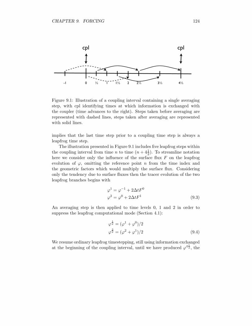
CHAPTER 9. FORCING 124
cpl cpl
! 1! 2! 3! 4!1 2-1 0
Figure 9.1: Illustration of a coupling interval containing a single averagingstep, with cpl identifying times at which information is exchanged withthe coupler (time advances to the right). Steps taken before averaging arerepresented with dashed lines, steps taken after averaging are representedwith solid lines.
implies that the last time step prior to a coupling time step is always aleapfrog time step.
The illustration presented in Figure 9.1 includes five leapfrog steps withinthe coupling interval from time n to time (n+ 41
2 ). To streamline notationhere we consider only the influence of the surface flux F on the leapfrogevolution of ϕ, omitting the reference point n from the time index andthe geometric factors which would multiply the surface flux. Consideringonly the tendency due to surface fluxes then the tracer evolution of the twoleapfrog branches begins with
ϕ1 = ϕ−1 + 2∆tF 0
ϕ2 = ϕ0 + 2∆tF 1 (9.3)
An averaging step is then applied to time levels 0, 1 and 2 in order tosuppress the leapfrog computational mode (Section 4.1):
ϕ1
2 = (ϕ1 + ϕ0)/2
ϕ3
2 = (ϕ2 + ϕ1)/2 (9.4)
We resume ordinary leapfrog timestepping, still using information exchangedat the beginning of the coupling interval, until we have produced ϕ4 1
2 , the
CHAPTER 9. FORCING 125
tracer at the end of the coupling interval:
ϕ2 1
2 = ϕ1
2 + 2∆tF 1 1
2
ϕ3 1
2 = ϕ1 1
2 + 2∆tF 2 1
2
ϕ4 1
2 = ϕ2 1
2 + 2∆tF 3 1
2 (9.5)
Summing (9.3) and (9.5), and making use of (9.4), the change in theaverage of the leapfrog branches over the coupling interval may be expressedin terms of the fluxes which span the coupling interval, as
1
2(ϕ4 1
2 + ϕ3 1
2 ) − 1
2(ϕ0 + ϕ−1) = ∆t(F 0 +
1
2F 1 + F 1 1
2 + F 2 1
2 + F 3 1
2 ) (9.6)
We accurately account for the fluxes passing through the ocean surface basedon this expression, with the exception of the very first coupling interval of arun which starts with a forward step, as in initial startup from climatology(we permit this one-time departure from strict conservation).
Under current practice, at the time this document is being prepared,the only temporal variation which may occur within the fluxes spanning acoupling interval is due to the use of an idealized diurnal cycle (Section 9.1),and due to the latent heat associated with the formation or melting of ice.The idealized diurnal cycle is conservative and used only when coupling isdaily. It does not change the amount of incoming SW, but only its tempo-ral distribution. Ice formation is only considered at the time of coupling,at which point both branches of the leap-frog time steps are modified, asexplained in Section 8.2, resulting in the addition of the QFLUX term of(8.22) to the right hand side of (9.6).
If another method of controlling the leapfrog computational mode is tobe used then the accounting of fluxes must be reconsidered. With use ofMatsuno steps an exact accounting is straightforward. An exact accountingof fluxes is more problematic with use of a Robert-Asselin time filter, asdiscussed in Leclair and Madec (2009).

Chapter 10
Parallel Implementation
POP has been designed to run effectively on a wide variety of high perfor-mance computing architectures. It has also been designed for portability, sothat no changes in the code itself are required to compile and run on a newarchitecture. This has been achieved by adhering to language standardsand by abstracting communication functions to support multiple messag-ing or other communication paradigms. No preprocessing directives areused, except to maintain some differences between the CCSM version andthe standalone POP, primarily due to coupling and CCSM shared code is-sues. In this chapter, details of the domain decomposition algorithms, thecommunication architecture and parallel I/O are described. Instructions onconfiguring POP inputs for performance are included in the POP User’sGuide.
10.1 Domain Decomposition
In order to compute efficiently on parallel architectures, work must be di-vided among each distributed computing node. POP, like many other cli-mate or fluid dynamics models, achieves this parallelism through domaindecomposition, dividing the gridded domain into pieces that each node cancompute relatively independently. To increase this independence, ghost cellsor halo regions are defined so that a node will have some information aboutstate variables on neighboring nodes (see Fig. 10.1). This enables the cal-culation on each node to proceed without communicating with other nodesuntil these regions need to be updated. In POP, using a halo width of twogrid cells will ensure that the entire baroclinic tendencies can be computedwithout any inter-node communication.
126

CHAPTER 10. PARALLEL IMPLEMENTATION 127
block_size_x
bloc
k_si
ze_y
nghost
ngho
st
block(i,j) block(i+1,j)block(i-1,j)
block(i,j-1)
block(i,j+1)
Figure 10.1: An illustration of a ghost cell or halo region, showing the halofor a particular block based on neighboring blocks.
Originally, POP decomposed the domain into single blocks per node.From POP 2.0 onward, POP has used a more flexible decomposition. Inthe new decomposition, the horizontal domain continues to be divided intoblocks, but multiple blocks can be distributed to each node, as shown inFigure 10.2. This structure enables the optimization of block size for cacheperformance. Multiple blocks on a node also provides a mechanism for hy-brid parallelism, in which a threaded parallelism (e.g. OpenMP) can be usedto distribute work within a multi-processor shared memory node, while mes-sage passing (e.g. MPI) is still used to communicate between distributednodes. Furthermore, different numbers of blocks can be assigned to eachnode to balance the computational load. Finally, this scheme permits theelimination of blocks which contain only land points. Such a structure pro-vides additional optimization tuning flexibility. The use of small blockscan eliminating more land, provide better load balancing and better perfor-mance on cache-based microprocessors. However, because each block has ahalo region, blocks that are too small have a high surface-to-volume ratioand communication and synchronization issues become dominant. Gener-ally, block sizes of 20-40 grid points in each direction appear to provide areasonable balance, though each computer is different.
POP supports three different schemes for distributing blocks among pro-cessors. All of them eliminate land blocks, but each represents options forbalancing the number of blocks per node.

CHAPTER 10. PARALLEL IMPLEMENTATION 128
ny_g
loba
l
nx_globallandocean
(a)
1
2 3
4
Processor 0 Processor 1
Processor 2 Processor 3
block_size_x
bloc
k_si
ze_y
(b)
1 2 3 4 5 6 7 8
9 10 11 12 13 14 15 16
17 18 19 20 21 22 23 24
25 26 27 28 29 30 31 32
block_size_x
bloc
k_si
ze_y
(c)
1 2 3 4 7 8
9 10
11
12
15
16
17 18 23 24
25 26 31 32
Processor 0 Processor 1
Processor 2 Processor 3
(d)
Figure 10.2: The POP subblocking decomposition, showing (a) the full do-main with shaded land cells, (b) a traditional single block Cartesian decom-position, (c) a subblock decomposition, and (d) a distribution of blocks inwhich land block have been eliminated and the computational load has beenbalanced.
CHAPTER 10. PARALLEL IMPLEMENTATION 129
10.1.1 Cartesian Distribution
The first option for block distribution is a simple Cartesian distribution. Inthis case, the sublocks in a domain are distributed according to their logicalposition in the domain with a two-dimensional rectangular decomposition,similar to that shown in Figure 10.2(b), except that the single blocks in thatfigure would correspond to the set of subblocks associated with those largeportions of the domain. No load balancing occurs and some nodes may beleft with no work to do if all blocks are land.
10.1.2 Rake Distribution
A second distribution scheme uses a simple rake algorithm to balance thework per node. The algorithm starts with the Cartesian distribution de-scribed above. Then an average number of blocks per node is computed. Ineach dimension, the algorithm starts with the first block in that dimensionand determines whether the number of blocks exceeds the mean and if so,blocks are passed on to the next node in line. This can be visualized as arake passing over each node and dragging excess work into the next available“hole”. In POP, additional constraints are placed on block movements, sothat if a block is moved once, it is not likely to be moved again and anotherblock is chosen for the move. This attempts to keep neighboring blocks aslocal as possible. Because the rake is performed in each logical directionseparately, there are instances where the algorithm can actually result in aworse load imbalance as blocks get raked into a corner. Also, if there arerelatively few blocks per node, load balancing is not very effective.
10.1.3 Space-filling Curve Distribution
A third distribution method is a partitioning algorithm based on space-fillingcurves (SFC). This algorithm draws a curve through the set of blocks in away that maintains locality and can more effectively balance both the com-putational load and the communications costs. Details can be found in Den-nis (2007). While the space-filling curve algorithm is supported for all resolu-tions, it is particularly effective at reducing the cost of high resolution simu-lations. Use of the SFC partitioning places restrictions on the size sub-blocksused by POP. In particular the size of the sub-blocks nxBlock and nyBlockmust be selected under the constraint that nbx = nxGlobal/nxBlock andnby = nyGlobal/nxBlock are integers such that nbx, nby ∈ 2n3m5p wheren,m, and p are integers and nxGlobal and nyGlobal refer to the global sizeof the horizontal computational grid.
CHAPTER 10. PARALLEL IMPLEMENTATION 130
As mentioned above, in addition to improving the computational loadbalance, SFC partitioning also has a tendency to improve the communicationload balance of POP (Dennis, 2007). In particular it randomizes networktraffic on machines with fixed interconnect topologies, resulting in decreasednetwork congestion and communication time.
10.2 Parallel I/O
In a parallel implementation, the lack of a parallel I/O subsystem creates aserial bottleneck that limits performance. Originally, POP created a parallelI/O system by gathering a single horizontal slice of a 3-D array onto oneof the I/O tasks and that task wrote the slice into a specified record of abinary direct-access file. This system was not always robust, due to localmachine I/O issues (e.g. system I/O buffers being overwritten by multiplewriters) and because this limits the number of I/O tasks and requires eachtask to keep a full global slice of the data. Finally, this implementation didnot support netCDF.
A new parallel I/O library, PIO, has been developed as a collaborativeeffort by NCAR/CISL, DOE/SciDAC and NCAR/CSEG. PIO was initiallydesigned to allow 0.1 POP to execute and write history and restart files onBlue Gene/L using less than 256 MB per MPI task due to better memorymanagement, relaxing the requirement for retaining a full global slice oneach I/O task.
Since that initial prototype version, PIO has developed into a gen-eral purpose parallel I/O library that currently supports netCDF (serial),pnetCDF and MPI IO and has been implemented throughout the entireCCSM system. PIO is a software interface layer designed to encapsulatethe complexities of parallel IO and to make it easier to replace the lowerlevel software backend. PIO calls are collective, an MPI communicator isset in a call to PIO init and all tasks associated with that communicatormust participate in all subsequent calls to PIO.
One of the key features of PIO is that it takes the model’s decompositionand redistributes it to an I/O “friendly” decomposition on the requestednumber of I/O tasks. In using the PIO library for netCDF or pnetCDFI/O, the user must specify the number of iotasks to be used, the strideor number of tasks between iotasks and whether the I/O will use the serialnetCDF or pnetCDF library. By varying the number of iotasks, the user caneasily reduce the serial I/O memory bottleneck (by increasing the numberof iotasks), even with the use of serial netCDF.
Bibliography
Adcroft, A., J.-M. Campin, P. Heimbach, C. Hill,and J. Marshall, 2005: MITgcm Manual. URLhttp://mitgcm.org/pelican/online documents/manual.html.
Adcroft, A., C. Hill, and J. Marshall, 1997: Representation of topographyby shaved cells in a height coordinate ocean model. Mon. Wea. Rev., 125,2293–2315.
Arakawa, A. and V. Lamb, 1977: Computational design of the basic dynam-ical processes of the ucla general circulation model. Methods of Computa-tional Physics, 17, 173.
Arfken, G., 1970: Mathematical Methods for Physicists. Academic, NewYork.
Boccaletti, G., R. Ferrari, and B. Fox-Kemper, 2007: Mixed layer in-stabilities and restratification. J. Phys. Oceanogr., 37, 2228–2250, doi:10.1175/JPO3101.1.
Briegleb, B., G. Danabasoglu, and W. Large, 2010: An over flow parameter-ization for the ocean component of the community climate system model.Tech. Rep. NCAR Tech. Note NCAR/TN-xxxx + STR, National Centerfor Atmospheric Research.
Brown, J. and K. A. Campana, 1978: An economical time-differencingscheme for numerical weather prediction. Mon. Weather Rev., 106, 1125–1136.
Bryan, K., 1969: A numerical method for the study of the world ocean. J.Comp. Phys., 4, 347–376.
Bryan, K., 1984: Accelerating the convergence to equilibrium of ocean-climate models. J. Phys. Oceanogr., 14, 666–673.
131
Capet, X., E. J. Campos, and A. M. Paiva, 2008a: Submesoscale activityover the Argentinian shelf. Geophysical Research Letters, 35, doi:ARTNL15605.
Capet, X., J. C. Mcwilliams, M. J. Mokemaker, and A. F. Shchepetkin,2008b: Mesoscale to submesoscale transition in the California currentsystem. Part I: Flow structure, eddy flux, and observational tests. J. Phys.Oceanogr., 38, 29–43, doi:DOI 10.1175/2007JPO3671.1.
Capet, X., J. C. Mcwilliams, M. J. Molemaker, and A. F. Shchepetkin,2008c: Mesoscale to submesoscale transition in the California current sys-tem. Part II: Frontal processes. J. Phys. Oceanogr., 38, 44–64, doi:DOI10.1175/2007JPO3672.1.
Capet, X., J. C. McWilliams, M. J. Molemaker, and A. F. Shchepetkin,2008d: Mesoscale to submesoscale transition in the California currentsystem. Part III: Energy balance and flux. J. Phys. Oceanogr., 38, 2256–2269, doi:DOI 10.1175/2008JPO3810.1.
Cox, M., 1987: Isopycnal diffusion in a z-coordinate ocean model. OceanModelling, 74, 1–5.
Danabasoglu, G., 2004: A comparison of global ocean general circulationmodel solutions obtained with synchronous and accelerated integrationmethods. Ocean Modelling, 7, 323–341.
Danabasoglu, G., R. Ferrari, and J. McWilliams, 2008: Sensitivity of anocean general circulation model to a parameterization of near-surface eddyfluxes. J. Climate, 21, 1192–1208, doi:10.1175/2007JCLI1508.1.
Danabasoglu, G., W. Large, and B. Briegleb, 2010: Climate impacts ofparameterized nordic sea overflows. submitted.
Danabasoglu, G., W. Large, J. Tribbia, P. Gent, B. Briegleb, andJ. McWilliams, 2006: Diurnal coupling in the tropical oceans of ccsm3. J.Climate, 19, 2347–2365.
Danabasoglu, G. and J. Marshall, 2007: Effects of vertical variations ofthickness diffusivity in an ocean general circulation model. Ocean Mod-elling, 18, 122–141, doi:10.1016/j.ocemod.2007.03.006.
Danabasoglu, G. and J. C. McWilliams, 1995: Sensitivity of the globalocean circulation to parameterizations of mesoscale tracer transports. J.Climate, 8, 2967–2987.
132
D’Azevedo, E., V. Eijkhout, and C. Romine, 1993: Lapack working note 56.conjugate gradient algorithms with reduced synchronization overhead ondistributed memory multiprocessors. Tech. Rep. Tech. Rep. CS-93-185,Computer Science Department, University of Tennessee, Knoxville, TN.
Dennis, J. M., 2007: Inverse space-filling curve partitioning of a global oceanmodel. Proceedings of IEEE International Parallel and Distributed Pro-cessing Symposium, doi: 10.1109/IPDPS.2007.370215.
Dewar, W., Y. Hsueh, T. J. McDougall, and D. Yuan, 1998: Calculation ofpressure in ocean simulations. J. Phys. Oceanogr., 28, 577–588.
Dukowicz, J., 2001: Reduction of density and pressure gradient errors inocean simulations. J. Phys. Oceanogr., 31, 1915–1921.
Dukowicz, J. and R. Smith, 1994: Implicit free-surface formulation of thebryan-cox-semtner ocean model. J. Geophys. Res., 99, 7991–8014.
Dukowicz, J. and R. Smith, 1997: Stochastic theory of compressible turbu-lent fluid transport. Phys. Fluids, 9, 3523–3529.
Dukowicz, J. K., R. D. Smith, and R. C. Malone, 1993: A reformulation andimplementation of the bryan-cox-semtner ocean model on the connectionmachine. J. Atmos. Ocean Tech., 14, 294–317.
Dutay, J.-C., et al., 2002: Evaluation of ocean model ventilation with cfc-11:comparison of 13 global ocean models. Ocean Modelling, 4, 89–120.
Eden, C. and R. Greatbatch, 2008: Towards a mesoscale eddy closure. OceanModelling, 20, 223–239.
Eden, C., M. Jochum, and G. Danabasoglu, 2009: Effects of different clo-sures for thickness diffusivity. Ocean Modelling, 26, 47–59.
England, M., 1995: The age of water and ventilation timescales in a globalocean model. J. of Phys. Oceanogr., 25, 2756–2777.
Farrow, D. and D. Stevens, 1995: A new tracer advection scheme for bryanand cox type ocean general circulation models. J. Phys. Oceanogr., 25,1731–1741.
Feistel, R. and E. Hagen, 1995: On the gibbs thermodynamic potential ofseawater. Prog. in Oceanogr., 36, 249–327.
133

Ferrari, R., J. McWilliams, V. Canuto, and M. Dubovikov, 2008: Parameter-ization of eddy fluxes near oceanic boundaries. J. Climate, 21, 2770–2789,doi:10.1175/2007JCLI1510.1.
Ferrari, R. and D. L. Rudnick, 2000: Thermohaline variability in the upperocean. Journal of Geophysical Research-Oceans, 105, 16 857–16 883.
Ferrari, R. and W. R. Young, 1997: On the development of thermohalinecorrelations as a result of nonlinear diffusive parameterizations. Journalof Marine Research, 55, 1069–1101.
Ferreira, D. and J. Marshall, 2006: Formulation and implementation of a“residual-mean” ocean circulation model. Ocean Modelling, 13, 86–107.
Ferreira, D., J. Marshall, and P. Heimbach, 2005: Estimating eddy stressesby fitting dynamics to observations using a residual-mean ocean circula-tion model and its adjoint. J. Phys. Oceanogr., 35, 1891–1910.
Fofonoff, N. and R. C. Millard, 1983: Algorithms for computation of fun-damental properties of seawater. UNESCO Technical Papers in MarineScience, 44, 53.
Fox-Kemper, B., G. Danabasoglu, R. Ferrari, S. M. Griffies, R. W. Hallberg,M. M. Holland, S. Peacock, and B. L. Samuels, 2010: Parameterizationof mixed layer eddies. III: Global implementation and impact on oceanclimate simulations, in preparation for Ocean Modelling.
Fox-Kemper, B., G. Danabasoglu, R. Ferrari, and R. W. Hallberg, 2008a:Parameterizing submesoscale physics in global climate models. CLIVARExchanges, 13, 3–5.
Fox-Kemper, B. and R. Ferrari, 2008: Parameterization of mixed layer ed-dies. Part II: Prognosis and impact. J. Phys. Oceanogr., 38, 1166–1179,doi:10.1175/2007JPO3788.1.
Fox-Kemper, B., R. Ferrari, and R. Hallberg, 2008b: Parameterization ofmixed layer eddies. Part I: Theory and diagnosis. J. Phys. Oceanogr., 38,1145–1165, doi:10.1175/2007JPO3792.1.
Garrett, C. and W. H. Munk, 1975: Space-time scales of internal waves: Aprogress report. J. Geophys. Res., 80, 291297.
Gent, P. and J. C. McWilliams, 1990: Isopycnal mixing in ocean circulationmodels. J. Phys. Oceanogr., 20, 150–155.
134

Gerdes, R., C. Koberle, and J. Willebrand, 1991: The influence of numeri-cal advection schemes on the results of ocean general circulation models.Climate Dynamics, 5, 211–226.
Gregg, M., 1987: Diapynal mixing in the thermocline: A review. J. Geophys.Res., 92, 52495286.
Gregg, M., 1989: Scaling turbulent dissipation in the thermocline. J. Geo-phys. Res., 94, 96869698.
Griffies, S., 1998: The gent-mcwilliams skew flux. J. Phys. Oceanogr., 28,831–841.
Griffies, S., A. Gnanadesikan, R. C. Pacanowski, V. Larichev, J. K. Dukow-icz, and R. D. Smith, 1998: Isoneutral diffusion in a z-coordinate oceanmodel. J. Phys. Oceanogr., 28, 805–830.
Griffies, S. and R. W. Hallberg, 2000: Biharmonic friction with asmagorinsky-like viscosity for use in large-scale eddy-permitting oceanmodels. Monthly Weather Review, 128, 2935–2946.
Griffies, S., R. C. Pacanowski, M. Schmidt, and V. Balaji, 2001: Tracerconservation with an explicit free surface method for z-coordinate oceanmodels. Monthly Weather Review, 129, 1081–1098.
Haine, T. W. N. and J. C. Marshall, 1998: Gravitational, symmetric andbaroclinic instability of the ocean mixed layer. J. Phys. Oceanogr., 28,634–658.
Haltiner, G. and R. Williams, 1980: Numerical Prediction and DynamicMeteorology. 2d ed., John Wiley and Sons, New York.
Hecht, M., W. Holland, and P. Rasch, 1995: Upwind-weighted advectionschemes for ocean tracer transport: An evaluation in a passive tracercontext. J. Geophys. Res., 100, 20 763–20 778.
Hibiya, T., M. Nagasawa, and Y. Niwa, 2006: Global mapping of di-aplycnal diffusivity in the deep ocean based on the results of expend-able current profiler (xcp) surveys. Geophys. Res. Lett., 33, L03 611,doi:10.1029/2005GL025 218.
Holland, W., F. Bryan, and J. Chow, 1998: Application of a third-orderupwind scheme in the ncar ocean model. J. Climate, 11, 1487–1493.
135

Hosegood, P., M. C. Gregg, and M. H. Alford, 2006: Sub-mesoscale lateraldensity structure in the oceanic surface mixed layer. Geophys. Res. Lett.,33, doi:10.1029/2006GL026 797.
Hundsdorfer, W. and R. Trompert, 1994: Method of lines and direct dis-cretization: a comparison for linear advection. Appl. Numer. Math., 13,469–490.
Jackett, D., T. McDougall, R. Feistel, D. Wright, and S. Griffies, 2006:Algorithms for density, potential temperature, conservative temperature,and the freezing temperature of seawater. J. of Atmos. and Oceanic Tech.,23, 1709–1728.
Jackett, D. and T. J. McDougall, 1995: Minimal adjustment of hydrographicprofiles to achieve static stability. J. of Atmos. and Oceanic Tech., 12,381–389.
Jayne, S., 2009: The impact of abyssal mixing parameterizations in an oceangeneral circulation model. J. Phys. Oceanogr., 39, 17561775.
Jayne, S. and L. C. S. Laurent, 2001: Parameterizing tidal dis-sipation over rough topography. Geophys. Res. Lett., 28, 811814,doi:10.1029/2000GL012 044.
Jochum, M., 2009: Simulated climate impacts of latitudinal vari-ations in diapycnal diffusivity. J. Geophys. Res., 114, C01 010,doi:10.1029/2008JC005 030.
Jochum, M., G. Danabasoglu, M. Holland, Y.-O. Kwon, and W. Large,2008: Ocean viscosity and climate. J. Geophys. Res., 113, C06 017,doi:10.1029/2007JC004 515.
Jochum, M. and J. Potemra, 2008: Sensitivity of tropical rainfall to bandasea diffusivity in the community climate system model. J. Climate, 21,6445–6454.
Killworth, P., D. Stainforth, D. Webb, and S. Paterson, 1991: The develop-ment of a free-surface bryan-cox-semtner ocean model. J. Phys. Oceanogr.,21, 1333–1348.
Large, W., G. Danabasoglu, S. Doney, and J. McWilliams, 1997: Sensitivityto surface forcing and boundary layer mixing in the ncar csm ocean model:Annual-mean climatology. J. Phys. Oceanogr., 27, 2418–2447.
136

Large, W., G. Danabasoglu, J. McWilliams, P. Gent, and F. Bryan, 2001:Equatorial circulation of a global ocean climate model with anisotropichorizontal viscosity. J. Phys. Oceanogr., 31, 518–536.
Large, W., J. McWilliams, and S. Doney, 1994: Oceanic vertical mixing:A review and a model with a nonlocal boundary layer parameterization.Reviews of Geophysics, 32, 363–403.
Laurent, L. S. and C. J. R. Garrett, 2002: The role of internal tides inmixing the deep ocean. J. Phys. Oceanogr., 32, 28822899.
Laurent, L. S. and J. D. Nash, 2004: An examination of the radiative anddissipative properties of deep ocean internal tides. Deep-Sea Res. II, 51,30293042, doi:10.1016/j.dsr2.2004.09.008.
Laurent, L. S., H. L. Simmons, and S. R. Jayne, 2002: Estimates of tidallydriven enhanced mixing in the deep ocean. Geophys. Res. Lett., 29, 2106,doi: 10.1029/2002GL015 633.
Leclair, M. and G. Madec, 2009: A conservative leapfrog time steppingmethod. Ocean Modelling, doi 10.1016/j.ocemod.2009.06.006.
Leonard, B., 1979a: A stable and accurate convective modeling procedurebased on quadratic upstream interpolation. Comp. Meth. in Appl. Eng.,19, 59–98.
Leonard, B., 1979b: The ultimate conservative difference scheme applied tounsteady one-dimensional advection. Comp. Meth. in Appl. Mech. Eng.,88, 17–74.
Madec, G. and M. Imbard, 1996: A global ocean mesh to overcome thenorth pole singularity. Climate Dyn., 12, 381–388.
Madec, G., M. Imbard, and C. Levy, 1998: Opa 8.1 ocean general circulationmodel reference manual. Tech. Rep. Note du Pole der modelisation number11, Institute Pierre-Simon Laplace (IPSL), France.
Mahadevan, A., A. Tandon, and R. Ferrari, 2009: Rapid changes in mixedlayer stratification driven by submesoscale instabilities and winds, in pressJ. Geophys. Res.
Maltrud, M., R. Smith, A. Semtner, and R. Malone, 1998: Global eddy-resolving ocean simulations driven by 1985-1995 atmospheric winds. J.Geophys. Res., 103, 825–830.
137

McDougall, T., 1987: Neutral surfaces. J. Phys. Oceanogr., 17, 1950–1964.
McDougall, T., D. Jackett, D. Wright, and R. Feistel, 2003: Accurate andcomputationally efficient algorithms for potential temperature and densityof seawater. J. of Atmos. and Oceanic Tech., 20, 730–741.
Murray, R., 1996: Explicit generation of orthogonal grids for ocean models.J. Comp. Phys., 126, 251–273.
NGDC, 2006: Two-minute gridded global relief data (etopo2v2). Tech. Rep.National Geophysical Data Center, National Oceanic and AtmosphericAdministration, U.S. Department of Commerce.
OCMIP, 2000: Ocean carbon model intercomparison project. URLhttp://www.ipsl.jussieu.fr/OCMIP/phase2/simulations/CFC/HOWTO-CFC.html.
Ohlmann, J., 2003: Ocean radiant heating in climate models. J. Climate,16, 1337–1351.
Osborn, T., 1980: Estimates of the local rate of vertical diffusion fromdissipation measurements. J. Phys. Oceanogr., 10, 8389.
Oschlies, A., 2002: Improved representation of upper-ocean dynamics andmixed layer depths in a model of the north atlantic on switching fromeddy-permitting to eddy-resolving grid resolution. J. Phys. Oceanogr., 32,2277–2298.
Pacanowski, R. and A. Gnanadesikan, 1998: Transient response in a z-level ocean model that resolves topography with partial cells. J. Phys.Oceanogr., 126, 3248–3270.
Pacanowski, R. and S. Griffies, 2000: The mom3 manual. Tech. rep., Geo-physical Fluid Dynamics Laboratory/NOAA, Princeton, NJ, USA.
Pacanowski, R. and S. Philander, 1981: Parameterization of vertical mixingin numerical models of the tropical oceans. J. Phys. Oceanogr., 11, 1443–1451.
Price, J. and M. Baringer, 1994: Outflows and deep water production bymarginal seas. Prog. Oceanogr., 33, 161–200.
Price, J. and J. Yang, 1998: Marginal sea overflows for climate simulations.Ocean Modeling and Parameterization, E. P. Chassignet and J. Verron,Eds., Kluwer Academic, 155–170.
138

Redi, M., 1982: Oceanic isopycnal mixing by coordinate rotation. J. Phys.Oceanogr., 12, 1154–1158.
Rudnick, D. L. and R. Ferrari, 1999: Compensation of horizontal tempera-ture and salinity gradients in the ocean mixed layer. Science, 283, 526–529.
Schopf, P. and A. Loughe, 1995: A reduced-gravity isopycnal ocean model:hindcasts of el nino. Monthly Weather Review, 123, 2839–2863.
Semtner, A., 1986: Finite-difference formulation of a world ocean model.Advanced Physical Oceanographic Numerical Modelling, J. O’Brien, Ed.,D. Reidel, Norwell, Mass., 187–202.
Simmons, H., S. R. Jayne, L. C. S. Laurent, and A. J. Weaver, 2004: Tidallydriven mixing in a numerical model of the ocean general circulation. OceanModelling, 6, 245263, doi:10.1016/S14635003(03)00 0118.
Smagorinsky, J., 1993: Some historical remarks on the use of nonlinear vis-cosities. Large Eddy Simulation of Complex Engineering and GeophysicalFlows, B. Galperin and S. Orszag, Eds., Cambridge University Press.
Smith, R., 1999: The primitive equations in the stochastic theory of adia-batic stratified turbulence. J. Phys. Oceanogr., 29, 1865–1880.
Smith, R., J. Dukowicz, and R. Malone, 1992: Parallel ocean general circu-lation modeling. Physica D., 60, 38–61.
Smith, R., S. Kortas, and B. Meltz, 1995: Curvilinear coordinates for globalocean models. Tech. Rep. LA-UR-95-1146, Los Alamos National Labora-tory.
Smith, R. and J. C. McWilliams, 2003: Anisotropic horizontal viscosity forocean models. Ocean Modelling, 5, 129–156.
Smith, W. and D. T. Sandwell, 1997: Global sea floor topography fromsatellite altimetry and ship depth soundings. Science, 277, 19561962,doi:10.1126/science.277.5334.1956.
St.Laurent, L. and R. Schmitt, 1999: The contribution of salt fingers tovertical mixing in the north atlantic tracer release experiment. J. Phys.Oceanogr., 29, 1404–1424.
Thiele, G. and J. Sarmiento, 1990: Tracer dating and ocean ventilation. J.Geophys. Res., 95, 9377–9391.
139
Thomas, L., 2005: Destruction of potential vorticity by winds. J. Phys.Oceanogr., 35, 2457–2466.
Thomas, L., 2008: Formation of intrathermocline eddies at ocean fronts bywind-driven destruction of potential vorticity. Dyn. Atmos. Ocean., 45,252–273.
Thomas, L. and C. M. Lee, 2005: Intensification of ocean fronts by down-front winds. J. Phys. Oceanogr., 35, 1086–1102.
Thomas, L. N. and R. Ferrari, 2008: Friction, frontogenesis, and the strat-ification of the surface mixed layer. J. Phys. Oceanogr., 38, 2501–2518,doi:DOI 10.1175/2008JPO3797.1.
Thomas, L. N., A. Tandon, and A. Mahadevan, 2008: Submesoscale pro-cesses and dynamics. Ocean Modeling in an Eddying Regime, M. Hechtand H. Hasumi, Eds., AGU Geophysical Monograph Series, Vol. 177, 17–38.
Visbeck, M., J. Marshall, T. Haine, and M. Spall, 1997: Specification ofeddy transfer coefficients in coarse-resolution ocean circulation models. J.Phys. Oceanogr., 27, 381–402.
Wajsowicz, R., 1993: A consistent formulation of the anisotropic stress ten-sor for use in models of the large-scale ocean circulation. J. Comp. Phys.,10, 333–338.
Walker, S., R. Weiss, and P. Salameh, 2009: Reconstructed his-tories of the annual mean atmospheric mole fractions for thehalocarbons cfc-11, cfc-12, cfc-113 and carbon tetrachloride. URLhttp://bluemoon.ucsd.edu/pub/cfchist/.
Webb, D., 1995: The vertical advection of momentum in bryan-cox-semtnerocean general circulation models. J. Phys. Oceanogr., 25, 3186–3195.
Whitehead, J., A. Leetmaa, and R. Knox, 1974: Rotating hydraulics ofstrait and sill flows. Geophys. Fluid Dyn., 6, 101–125.
Williams, G., 1972: Friction term formulation and convective instability ina shallow atmosphere. J. Atmos. Sci., 29, 870–876.
Wu, W., G. Danabasoglu, and W. Large, 2007: On the effects of param-eterized mediterranean overflow on north atlantic ocean circulation andclimate. Ocean Modelling, 19, 31–52, doi:10.1016/j.ocemod.2007.06.003.
140