the pascagoula river - champs lab
TRANSCRIPT

A HIGH-RESOLUTION STORM SURGE MODEL FOR THE PASCAGOULA REGION, MISSISSIPPI
by
NAEKO TAKAHASHI B.S. Chuo University, JAPAN, 2001
A thesis submitted in partial fulfillment of the requirements for the degree of Master of Science
in the Department of Civil, Environmental and Construction Engineering in the College of Engineering and Computer Science
at the University of Central Florida Orlando, Florida
Fall Term 2008

ii
© 2008 Naeko Takahashi

iii
ABSTRACT
The city of Pascagoula and its coastal areas along the United States Gulf Coast have
experienced many catastrophic hurricanes and were devastated by high storm surges
caused by Hurricane Katrina (August 23 to 30, 2005). The National Hurricane Center
reported high water marks exceeding 6 meters near the port of Pascagoula with a near 10-
meter high water mark recorded near the Hurricane Katrina landfall location in Waveland,
MS. Although the Pascagoula River is located 105 km east of the landfall location of
Hurricane Katrina, the area was devastated by storm surge-induced inundation because of
its low elevation.
Building on a preliminary finite element mesh for the Pascagoula River, the work
presented herein is aimed at incorporating the marsh areas lying adjacent to the Lower
Pascagoula and Escatawpa Rivers for the purpose of simulating the inland inundation
which occurred during Hurricane Katrina. ADCIRC-2DDI (ADvanced CIRCulation
Model for Shelves, Coasts and Estuaries, Two-Dimensional Depth Integrated) is
employed as the hydrodynamic circulation code. The simulations performed in this study
apply high-resolution winds and pressures over the 7-day period associated with
Hurricane Katrina. The high resolution of the meteorological inputs to the problem
coupled with the highly detailed description of the adjacent inundation areas will provide
an appropriate modeling tool for studying storm surge dynamics within the Pascagoula
River. All simulation results discussed herein are directed towards providing for a full

iv
accounting of the hydrodynamics within the Pascagoula River in support of ongoing
flood/river forecasting efforts.
In order to better understand the hydrodynamics within the Pascagoula River when driven
by an extreme storm surge event, the following tasks were completed as a part of this
study:
1) Develop an inlet-based floodplain DEM (Digital Elevation Model) for the Pascagoula
River. The model employs topography up to the 1.5-meter contour extracted from the
Southern Louisiana Gulf Coast Mesh (SL15 Mesh) developed by the Federal Emergency
Management Agency (FEMA).
2) Incorporate the inlet-based floodplain model into the Western North Atlantic Tidal
(WNAT) model domain, which consists of the Gulf of Mexico, the Caribbean Sea, and
the entire portion of the North Atlantic Ocean found west of the 60 degree West meridian,
in order to more fully account for the storm surge dynamics occurring within the
Pascagoula River. This large-scale modeling approach will utilize high-resolution wind
and pressure fields associated with Hurricane Katrina, so that storm surge hydrographs
(elevation variance) at the open-ocean boundary locations associated with the localized
domain can be adequately obtained.
3) Understand the importance of the various meteorological forcings that are attributable
to the storm surge dynamics that are setup within the Pascagoula River. Different

v
implementations of the two model domains (large-scale, including the WNAT model
domain; localized, with its focus concentrated solely on the Pascagoula River) will
involve the application of tides, storm surge hydrographs and meteorological forcing
(winds and pressures) in isolation (i.e., as the single forcing mechanism) and collectively
(i.e., together in combination).
The following conclusions are drawn from the research presented in this thesis: 1)
Incorporating the marsh areas into the preliminary in-bank mesh provides for significant
improvement in the astronomic tide simulation; 2) the large-scale modeling approach (i.e.,
the localized floodplain mesh incorporated into the WNAT model domain) is shown to be
most adequate towards simulating storm surge dynamics within the Pascagoula River.
Further, we demonstrate the utility of the large-scale model domain towards providing
storm surge hydrographs for the open-ocean boundary of the localized domain. Only
when the localized domain is forced with the storm surge hydrograph (generated by the
large-scale model domain) does it most adequately capture the full behavior of the storm
surge. Finally, we discover that while the floodplain description up to the 1.5-m contour
greatly improves the model response by allowing for the overtopping of the river banks, a
true recreation of the water levels caused by Hurricane Katrina will require a floodplain
description up to the 5-m contour.

vi
ACKNOWLEDGMENTS
As I finalized my work at the University of Central Florida, I realized that I am blessed
with invaluable support. First of all, I am sincerely grateful to Dr. Scott C. Hagen for
directing me throughout the process of this graduate research and for his invaluable
suggestions. In addition, I appreciate his patience and understanding during my time as a
member of the CHAMPS (Coastal Hydrodynamics, Analysis, Modeling and Predictive
Simulations) Laboratory. I would also like to thank Drs. Manoj Chopra and Gour-Tsyh
Yeh for agreeing to serve on my committee. I have also experienced the joy of learning
and understanding science and engineering in their classrooms, and this will continue to
help me in my career as an engineer. Also, I would like to emphasize that this thesis is a
collaborative effort with Qing Wang who has been working with me on this project. I am
thankful for her intelligence and friendship over the past two years.
Further, I gratefully acknowledge the help of all of current members in CHAMPS Lab:
Peter Bacopoulos for overseeing my studies with his qualified suggestions. His
participation allowed us to overcome and learn from the many obstacles that Qing and I
encountered in completing this work. He also helped me to improve my English skills
since I first joined the lab as an ESOL student; Stephen Medeiros for sharing his
knowledge as a professional engineer and serving as my thesis editor; David Coggin,
Derek Giardino, Alfredo Ruiz, and Hitoshi Tamura. I wish them success in their
academics and bright futures after they graduate. I also thank former lab members, Yuji

vii
Funakoshi, Michael Parrish, Mike Salisbury, and Satoshi Kojima, for their additional
advice.
I extend special thanks to Mr. David Welch, Mr. Dave Reed and Mr. Dave Ramirez of
the Lower Mississippi River Forecast Center for their cooperation in providing the cross
sectional data and background papers that were used in the preparation of this project.
Last but not least, I am very grateful to my parents for allowing me to study abroad. My
family (especially my newborn niece) and friends always cheer me up. Without the
generous thoughts of these individuals, this investigation would not have been possible.
This research was funded in part by award NA04NWS4620013 from the National
Oceanic and Atmospheric Administration (NOAA), U.S. Department of Commerce. The
statements, findings, conclusions and recommendations are those of the author and do not
necessarily reflect those of the NOAA, the Department of Commerce and its affiliates.

viii
TABLE OF CONTENTS
LIST OF FIGURES ........................................................................................................... xi
LIST OF TABLES........................................................................................................... xvi
LIST OF ABBREVIATIONS......................................................................................... xvii
CHAPTER 1. INTRODUCTION .................................................................................. 1
1.1 Advanced Circulation Model.................................................................................... 5
1.2 The WNAT (Western North Atlantic Tidal) Model Domain ................................... 6
1.3 The Pascagoula River ............................................................................................... 9
1.4 Hurricane Katrina.................................................................................................... 11
1.4.1 History of the Storm......................................................................................... 11
1.4.2 Reported High Water Marks............................................................................ 13
CHAPTER 2. LITERATURE REVIEW ..................................................................... 22
2.1 Storm Surge Generation.......................................................................................... 22
2.2 Storm Surge Modeling............................................................................................ 25
CHAPTER 3. FINITE ELEMENT MESH DEVELOPMENT.................................... 31
3.1 Preliminary In-bank Mesh ...................................................................................... 31
3.2 Floodplain Mesh Development............................................................................... 35
CHAPTER 4. MODEL DESCRIPTION ..................................................................... 43
4.1 Hydrodynamic Model ............................................................................................. 43
ix
4.2 Tropical Wind Stress and Pressure Field ................................................................ 50
CHAPTER 5. MODEL SETUP ................................................................................... 55
5.1 Model Forcings ....................................................................................................... 55
5.1.1 Astronomic Tides............................................................................................. 55
5.1.2 Wind and Pressure ........................................................................................... 57
5.1.3 Storm Surge Hydrograph ................................................................................. 61
5.2 Model Parameters ................................................................................................... 62
CHAPTER 6. MODEL RESULTS.............................................................................. 65
6.1 Astronomic Tide Simulation (Experiments 1 and 2) .............................................. 66
6.2 Storm Surge Model ................................................................................................. 74
6.2.1 WNAT-based Model and Storm Surge Hygrograph Extraction (Experiments 3
and 4) ........................................................................................................................ 74
6.2.2 Inlet-based Model with Storm Surge Hydrographs (Experiments 5 and 6)..... 84
6.2.3 Inlet-based Model with Storm Surge Hydrograph and Meteorological Forcings
(Experiments 7)......................................................................................................... 92
6.2.4 Comparison of WNAT-based Model (Experiment 4) and Inlet-based Model
(Experiment 7) ........................................................................................................ 100
6.2.5 Historical Data Verification........................................................................... 106
CHAPTER 7. CONCLUSIONS AND FUTURE WORK ......................................... 110
7.1 Conclusions........................................................................................................... 110
7.2 Future Work .......................................................................................................... 112
APPENDIX A. SAFFIR SIMPSON HURRICANE SCALE................................... 115
APPENDIX B. STORM SURGE HEIGHT DATA SET ........................................ 117
APPENDIX C. TIDAL CONSTITUENTS EMPLOYED BY ADCIRC-2DDI...... 121

x
APPENDIX D. ADCIRC-2DDI INPUT FILE: SINGLE METROLOGICAL INPUT
FILE (FORT.22) USED FOR WNAT-53K MESH DOMAIN ...................................... 126
LIST OF REFERENCES................................................................................................ 128
xi
LIST OF FIGURES
Figure 1.1 Comprehensive Pascagoula River Mesh (shown in red) overlaid on aerial
photography of the region (image courtesy of Google Earth). ........................................... 3
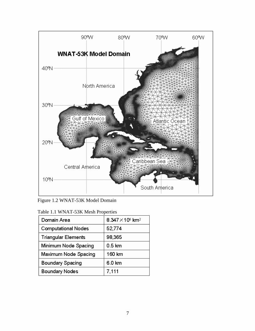
Figure 1.2 WNAT-53K Model Domain.............................................................................. 7
Figure 1.3 WNAT-53K Model Bathymetry Contours. Positive values represent depths
below NAVD88 .................................................................................................................. 8
Figure 1.4 Study Area and Gages in Lower Pascagoula................................................... 10
Figure 1.5 Best Track Position for Hurricane Katrina, 23-30 August 2005..................... 15
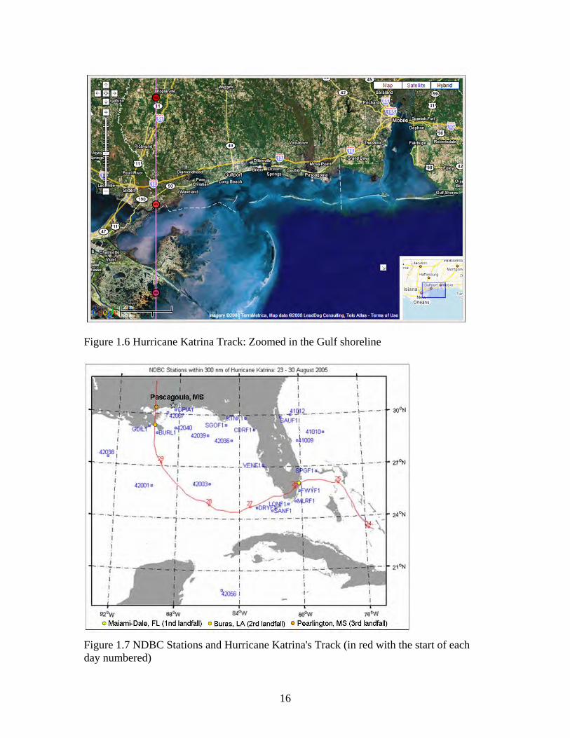
Figure 1.6 Hurricane Katrina Track: Zoomed in the Gulf shoreline ................................ 16
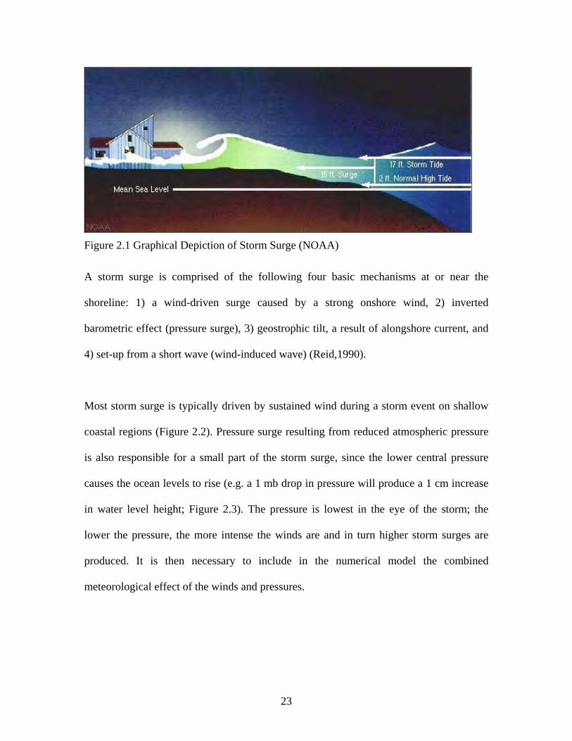
Figure 1.7 NDBC Stations and Hurricane Katrina's Track (in red with the start of each
day numbered) .................................................................................................................. 16
Figure 1.8 NDBC Station 42040: (Top) Winds (Anemometer Height 5m) and Sea-level
Pressure/ (Bottom) Significant Wave Height and Dominant Period ................................ 17
Figure 1.9 NDBC Station 42007: (Top) Winds (Anemometer Height 5m) and Sea-level
Pressure/ (Bottom) Significant Wave Height and Dominant Period ................................ 18
Figure 1.10 Hurricane Katrina (2005) storm surge height measurements and Hurricane
Camille (1969) high water mark profile (Fritz, 2008) ...................................................... 19
Figure 1.11 Foods in Pascagoula, MS over 1/2 mile inland (Weather Underground, Inc)
........................................................................................................................................... 20
Figure 1.12 Highway 90 (rear) and partially damaged railway (front) on the West
Pascagoula River (USGS Center for Coastal & Watershed Studies) ............................... 20
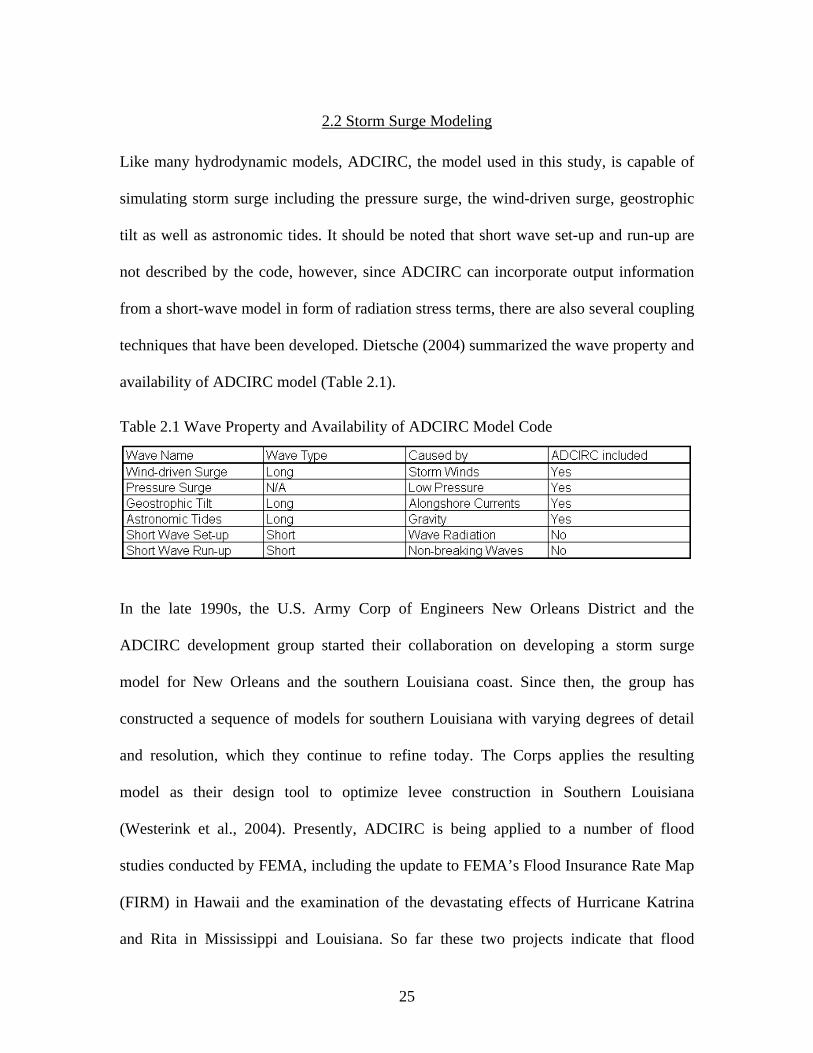
Figure 2.1 Graphical Depiction of Storm Surge (NOAA)................................................ 23
Figure 2.2 Storm Surge cased by Wind and Pressure (Simmon, NASA Goddard Space
Flight Center) .................................................................................................................... 24
Figure 2.3 Inverted Barometric Effect (http://www.oc.nps.edu/) ..................................... 24
Figure 3.1 SL15 Mesh: Zoomed in the Pascagoula River Region.................................... 33
Figure 3.2 Pascagoula River Preliminary In-bank Mesh (Mesh A).................................. 34
Figure 3.3 Figure 3.4 Satellite Images of Marsh Areas in the Lower Pascagoula and
Escatawpa Rivers (image courtesy of Google Earth) ....................................................... 35
Figure 3.5 SL15 Mesh: Topography Contours Up to 1.5 m above NAVD88.................. 36

xii
Figure 3.6 Inlet-based 1.5 m Floodplain Mesh (FP1.5_INLET_A; Used for Astronomic
Tide Simulation) ............................................................................................................... 37
Figure 3.7 Inlet-based 1.5 m Floodplain Mesh (FP1.5_INLET_A; Typically for
Astronomic Tide Simulation) ........................................................................................... 38
Figure 3.8 Inlet-based 1.5 m Floodplain Mesh (FP1.5_INLET_B; River Islands Meshed
Over) ................................................................................................................................. 40
Figure 3.9 Coastline Boundary Comparisons ................................................................... 40
Figure 3.10 WNAT-based 1.5 m Floodplain Mesh (FP1.5_WNAT_A) .......................... 41
Figure 3.11 WNAT-based 1.5 m Floodplain Mesh (FP1.5_WNAT_B; Barrier Islands
Meshed Over).................................................................................................................... 41
Figure 4.1 Planetary Boundary Layer (http://www.shodor.org)....................................... 50
Figure 5.1 Wind Field Extent Shown Relative to the WNAT-Pascagoula Mesh. Note that
all nodes of the mesh are located within the extent of the wind field............................... 58
Figure 5.2 Direction of the wind....................................................................................... 60
Figure 5.3 Magnitude of the wind..................................................................................... 60
Figure 6.1 Historical Data Stations................................................................................... 68
Figure 6.2 Resyntheses of historical and model tidal constituents, corresponding to the
stations located at Pascagoula Point, Mississippi Sound, MS and Pascagoula, MS......... 70
Figure 6.3 Resyntheses of historical and model tidal constituents, corresponding to the
stations located at Pascagoula River Mile 1, MS and West Pascagoula at Gautier, MS. . 71
Figure 6.4 Resyntheses of historical and model tidal constituents, corresponding to the
stations at Pascagoula River at Cumbest Bluff and Graham Ferry, MS........................... 72
Figure 6.5 Resyntheses of historical and model tidal constituents, corresponding to the
station located at Escatawpa River at I-10 near Orange Grove, MS. ............................... 73
Figure 6.6 Ninety-nine Open Ocean Boundary Nodes of FP1.5_INLET Model ............. 77
Figure 6.7 Storm Surge Hydrograph at Open-ocean Boundary Node 1 ........................... 77
Figure 6.8 Storm Surge Hydrograph at Open-ocean Boundary Node 10 ......................... 78
Figure 6.9 Storm Surge Hydrograph at Open-ocean Boundary Node 20 ......................... 78
Figure 6.10 Storm Surge Hydrograph at Open-ocean Boundary Node 30 ....................... 79
Figure 6.11 Storm Surge Hydrograph at Open-ocean Boundary Node 40 ....................... 79
Figure 6.12 Storm Surge Hydrograph at Open-ocean Boundary Node 50 ....................... 80

xiii
Figure 6.13 Storm Surge Hydrograph at Open-ocean Boundary Node 60 ....................... 80
Figure 6.14 Storm Surge Hydrograph at Open-ocean Boundary Node 70 ....................... 81
Figure 6.15 Storm Surge Hydrograph at Open-ocean Boundary Node 80 ....................... 81
Figure 6.16 Storm Surge Hydrograph at Open-ocean Boundary Node 90 ....................... 82
Figure 6.17 Storm Surge Hydrograph at Open-ocean Boundary Node 99 ....................... 82
Figure 6.18 Maximum Envelop of Water (Top) FP1.5_WNAT model forced by global
wind and pressure; (Middle left& right) Insets of Gulf Coast in 53K and FP1.5_WNAT
model; (Bottom left& right) Insets of Pascagoula Estuary in 53K and FP1.5_WNAT
model................................................................................................................................. 83
Figure 6.19 Model Storm Surge Hydrograph at Graveline Bayou Entrance, MS ............ 86
Figure 6.20 Model Storm Surge Hydrograph at West Pascagoula @ Highway 90 @
Gautier, MS....................................................................................................................... 86
Figure 6.21 Model Storm Surge Hydrograph at Escatawpa, Pascagoula River, MS........ 87
Figure 6.22 Model Storm Surge Hydrograph at Martin Bluff, West Pascagoula River, MS
........................................................................................................................................... 87
Figure 6.23 Model Storm Surge Hydrograph at Graham Fish Camp, Pascagoula River,
MS..................................................................................................................................... 88
Figure 6.24 Model Storm Surge Hydrograph at Poticaw Lodge, West Pascagoula River,
MS..................................................................................................................................... 88
Figure 6.25 Model Storm Surge Hydrograph at Pascagoula River @ Cumbest Bluff, MS
........................................................................................................................................... 89
Figure 6.26 Model Storm Surge Hydrograph at Graham Ferry, Ascagoula River, MS ... 89
Figure 6.27 Model Storm Surge Hydrograph at Moss Point, Escatawpa River, MS ....... 90
Figure 6.28 Model Storm Surge Hydrograph at Pascagoula River @ Mile 1 @
Pascagoula, MS................................................................................................................. 90
Figure 6.29 Maximum Envelop of Water (Top left) FP1.5_INLET model forced by storm
surge hydrograph obtained from 53K mesh domain; (Top right) FP1.5_INLET model
forced by storm surge hydrograph obtained from 53K mesh domain; (Bottom) Difference
of two models.................................................................................................................... 91
Figure 6.30 Model Storm Surge Hydrograph at Graveline Bayou Entrance, MS ............ 94

xiv
Figure 6.31 Model Storm Surge Hydrograph at West Pascagoula @ Highway 90 @
Gautier, MS....................................................................................................................... 94
Figure 6.32 Model Storm Surge Hydrograph at Escatawpa, Pascagoula River, MS........ 95
Figure 6.33 Model Storm Surge Hydrograph at Martin Bluff, West Pascagoula River, MS
........................................................................................................................................... 95
Figure 6.34 Model Storm Surge Hydrograph at Graham Fish Camp, Pascagoula River,
MS..................................................................................................................................... 96
Figure 6.35 Model Storm Surge Hydrograph at Poticaw Lodge, West Pascagoula River,
MS..................................................................................................................................... 96
Figure 6.36 Model Storm Surge Hydrograph at Pascagoula River @ Cumbest Bluff, MS
........................................................................................................................................... 97
Figure 6.37 Model Storm Surge Hydrograph at Pascagoula River @ Graham Ferry, MS
........................................................................................................................................... 97
Figure 6.38 Model Storm Surge Hydrograph at Moss Point, Escatawpa River, MS ....... 98
Figure 6.39 Model Storm Surge Hydrograph at Escatawpa River @ 1-10 near Orange
Grove, MS......................................................................................................................... 98
Figure 6.40 Maximum Envelop of Water (Top left) FP1.5_INLET model forced by storm
surge hydrograph obtained from FP1.5_WNAT mesh domain; (Top right) FP1.5_INLET
model forced by storm surge hydrograph obtained from FP1.5_WNAT mesh domain plus
wind and pressure; (Bottom) Difference of two models................................................... 99
Figure 6.41 Model Storm Surge Hydrograph at Graveline Bayou Entrance, MS .......... 101
Figure 6.42 Model Storm Surge Hydrograph at West Pascagoula @ Highway 90 @
Gautier, MS..................................................................................................................... 101
Figure 6.43 Model Storm Surge Hydrograph at Escatawpa, Pascagoula River, MS...... 102
Figure 6.44 Model Storm Surge Hydrograph at Martin Bluff, West Pascagoula River, MS
......................................................................................................................................... 102
Figure 6.45 Model Storm Surge Hydrograph at Graham Fish Camp, Pascagoula River,
MS................................................................................................................................... 103
Figure 6.46 Model Storm Surge Hydrograph at Poticaw Lodge, West Pascagoula River,
MS................................................................................................................................... 103

xv
Figure 6.47 Model Storm Surge Hydrograph at Pascagoula River @ Cumbest Bluff, MS
......................................................................................................................................... 104
Figure 6.48 Model Storm Surge Hydrograph at Pascagoula River @ Graham Ferry, MS
......................................................................................................................................... 104
Figure 6.49 Model Storm Surge Hydrograph at Moss Point, Escatawpa River, MS ..... 105
Figure 6.50 Model Storm Surge Hydrograph at Escatawpa River @ 1-10 near Orange
Grove, MS....................................................................................................................... 105
Figure 6.51 Historical Water Stage and Model Storm Surge Hydrograph Comparison at
Pascagoula, MS............................................................................................................... 107
Figure 6.52 Historical Water Stage and Model Storm Surge Hydrograph Comparison at
West Pascagoula @ Highway 90 @ Gautier, MS........................................................... 108
Figure 6.53 Historical Water Stage and Model Storm Surge Hydrograph Comparison at
Pascagoula River @ Cumbest Bluff, MS ....................................................................... 108
Figure 6.54 Historical Water Stage and Model Storm Surge Hydrograph Comparison at
Graham Ferry, Pascagoula River, MS ............................................................................ 109
Figure 6.55 Historical Water Stage and Model Storm Surge Hydrograph Comparison at
Escatawpa River @ 1-10 near Orange Grove, MS ......................................................... 109
Figure 7.1 SL15: Up to 5.0 m above MSL Contours...................................................... 114

xvi
LIST OF TABLES
Table 1.1 WNAT-53K Mesh Properties ............................................................................. 7
Table 1.2 Legend for Figure 1.8 and Figure 1.9 ............................................................... 19
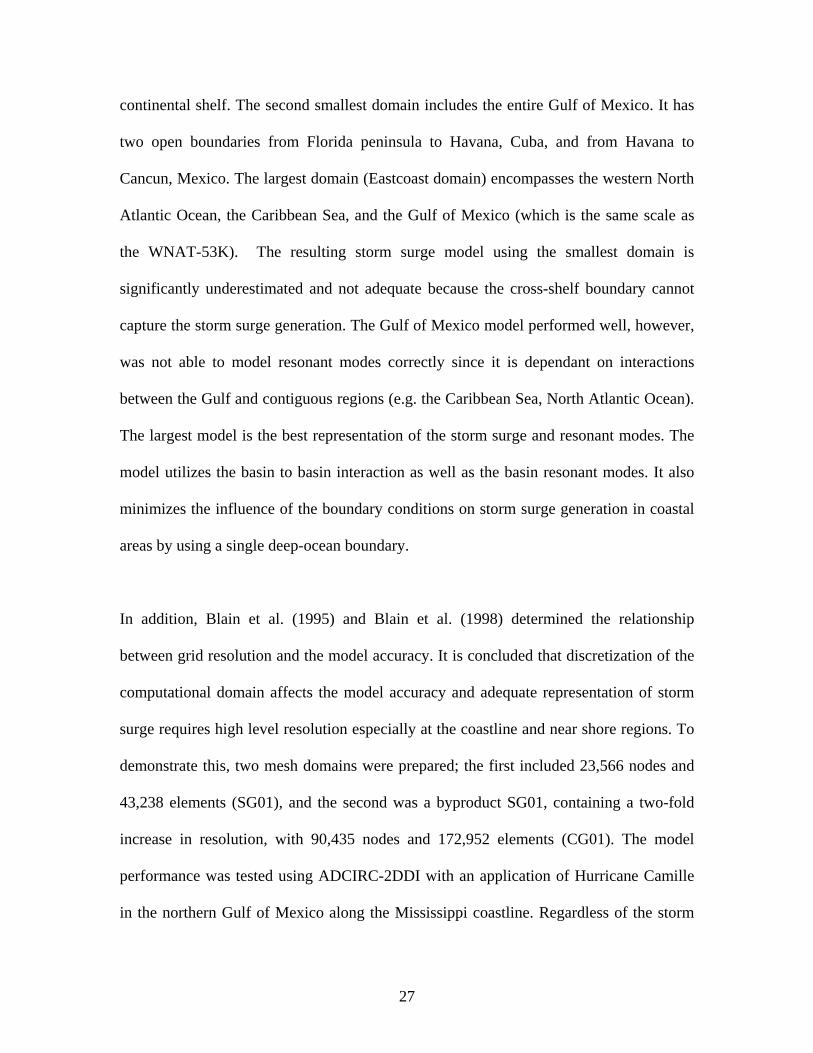
Table 2.1 Wave Property and Availability of ADCIRC Model Code .............................. 25
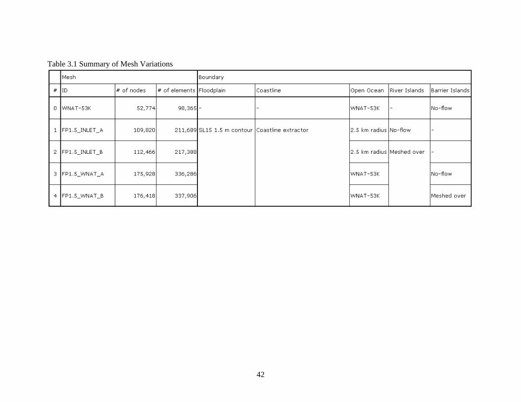
Table 3.1 Summary of Mesh Variations ........................................................................... 42
Table 5.1 Seven tidal constituents used to force the WNAT-based model ...................... 56
Table 5.2 Model Parameters ............................................................................................. 64
Table 6.1 Simulation Table............................................................................................... 66
Table 6.2 Historical Data Stations .................................................................................... 68
Table 7.1 Legend for Fort.22 .......................................................................................... 126

xvii
LIST OF ABBREVIATIONS
1D One Dimensional
2D Two Dimensional
ADCIRC-2DDI Advanced Circulation Model for Oceanic, Coastal, and
Estuarine Waters (Two-Dimensional, Depth-Integrated
Option)
CPP Carte Parallelogrammatique Project
DEM Digital Elevation Model
FEMA Federal Emergency Management Agency
FIRM Flood Insurance Rate Map
GIS Geographic Information System
GPS Global Positioning System
GWCE Generalized Wave Continuity Equation
LMRFC Lower Mississippi River Forecast Center
LTEA Localized Truncation Error Analysis
MEOW Maximum Envelope of Water
NAVD 88 North American Vertical Datum of 1988
NOAA National Oceanic and Atmospheric Administration
NOS National Ocean Service
RMS Root Mean Square
SLOSH Sea, Lake and Overland Surges from Hurricanes model
SMS Surface-water Modeling System
USGS United States Geological Survey

1
CHAPTER 1. INTRODUCTION
Disaster prediction and protection has been recognized as one of the most important and
critical issues in today’s world since natural disasters such as earthquakes, floods, and
hurricanes impact our lives and economies. Therefore, the nation’s emergency
management systems must be capable of handling and preparing future regional master
plans, insurance plans, and emergency evacuation plans. It is the duty of civil engineers
and scientists to provide reliable resources and solutions to assist in this effort to serve
the public good.
This study presents simulated storm surges for the Pascagoula River, located in lower
Mississippi along the Gulf of Mexico, caused by Hurricane Katrina (2005). The
Pascagoula River is located 105 km east of the landfall location of Hurricane Katrina;
despite the distance from the eye of the storm, the area was inundated by an approximate
5-meter storm surge due to its vast low-lying coastal plain. The majority of the fatalities
in Mississippi (reported as 238; Knabb et al., 2005) were directly caused by the storm
surge. This study is motivated by the absence of an existing model that can accurately
describe storm tide propagation up the Pascagoula River and over its banks into the
adjacent floodplains. All research presented herein is directed towards providing for a full
accounting of the hydrodynamics within the Pascagoula River in support of ongoing
flood/river forecasting efforts.
The University of Central Florida is cooperating with the Hydrology Laboratory of the
NWS Office of Hydrologic Development and the Lower Mississippi River Forecast

2
Center (LMRFC) to develop a two-dimensional storm tide model for the Pascagoula
River. The major goals of this overall project are to: 1) include the Pascagoula River in a
modification of an existing model domain encompassing the entire east coast of the
United States, Gulf of Mexico and Caribbean Sea such that astronomic tides and storm
surge can be accurately modeled; 2) develop localized domain for the Pascagoula River
that will produce results comparable to the large-scale domain from Goal 1. This research
will result in a model that more completely accounts for the hydraulic conditions in flood
forecasts and flood forecast mapping in the study area.
Recently, as the first report of this project, Wang (2008) has presented a preliminary
finite element model domain for the Pascagoula River, which is capable of accurately
describing the hydrodynamics of the astronomic tides within the banks of the Pascagoula
River (Figure 1.1). This portion of the study concluded that: 1) the comprehensive
Pascagoula River model domain is able to reproduce the hydrodynamics for in-bank flow
driven by astronomic tides; 2) the tides propagate up the river system to Graham Ferry,
55 km (34.5 miles) upstream from the inlets. To expand on the in-bank mesh used by
Wang (2008), it is presented in this thesis the refinement of the comprehensive model
domain to include the inundation areas, mainly those contained within the Lower
Pascagoula and Escatawpa regions. This floodplain model domain will then be applied in
tidal and storm surge simulations in order to investigate the role of the inundation areas in
tidally driven processes and storm surge dynamics in the Pascagoula River. Additional
experimentation with the floodplain model domain will realize knowledge of the tidal and
meteorological forcings and their influence on the local system response.

3
Figure 1.1 Comprehensive Pascagoula River Mesh (shown in red) overlaid on aerial photography of the region (image courtesy of Google Earth).
Therefore, as the second report of this project, three major objectives have been
completed:
1) Develop a Pascagoula floodplain model domain that includes the inundation areas up
to the 1.5-meter NAVD88 contour.
2) Incorporate the Pascagoula floodplain model domain in the Western North Atlantic
Tidal (WNAT) model domain (Figure 1.2), which encompasses the entire east coast of
the United States, Gulf of Mexico and Caribbean Sea, such that astronomic tides and
storm surge can be simulated using a large-domain modeling approach.

4
3) Apply the large-scale (WNAT-based) and local-scale (inlet-based) model domains in a
variety of tidal and storm surge simulations. Different implementations of the two model
domains will involve the application of tides, storm surge hydrographs and
meteorological forcing (winds and pressures) in isolation (i.e., as the single forcing
mechanism) and collectively (i.e., together in combination). The knowledge gained from
these experiments will yield knowledge of the forcing mechanisms for the Pascagoula
River and the manner in which they are incorporated into a numerical model.
The study presented herein provides storm surge simulation results and floodplain
mapping values for the Pascagoula River that are valuable to many applied modeling
efforts for various topics. This study serves as a thesis in partial fulfillment of the
requirements for a Master of Science degree in Civil Engineering at the University of
Central Florida in the fall semester 2008. The project as a whole is in pursuit of an
operational forecasting model for the Pascagoula region that was conducted in
conjunction with LMRFC. The computations were performed in the UCF CHAMPS
Laboratory.

5
1.1 Advanced Circulation Model
Astronomic and meteorological tides are calculated using the ADCIRC-2DDI (ADvanced
CIRCulation Model for Shelves, Coasts and Estuaries, Two-Dimensional Depth
Integrated) hydrodynamic circulation code (Westerink, Blain, Luettich, & Scheffner,
1994). This finite element based model solves the shallow water equations in their full
nonlinear form. It can be forced with elevation boundary conditions, flux boundary
conditions, and tidal potential terms, all of which result in the full simulation of
astronomic tides. In addition, dynamic wind fields for a given hurricane or tropical storm
event (e.g. Hurricane Katrina) are converted to spatially variable and time-dependent
wind surface stresses and then incorporated into the ADCIRC-2DDI model along with
atmospheric pressure variations that permit for the simulation of a storm surge. Further,
the ADCIRC-2DDI model allows for wetting and drying of nearshore and inland
elements to simulate flood inundation and recession.
ADCIRC-2DDI solves the linear algebraic equations that result from the finite element
discretization of the GWCE (Generalized Wave Continuity Equation) formulation using
pre-conditioned conjugate gradient solvers. The number of iterations required per time
step is very low and the computational cost in terms of CPU and memory increase
linearly with the number of nodes. This allows the application of grids with very large
numbers of nodes. To further enhance the computational capability of ADCIRC-2DDI, a
parallel version has been developed and is installed on multiple high performance
computing clusters in the UCF CHAMPS Laboratory.

6
1.2 The WNAT (Western North Atlantic Tidal) Model Domain
Previous efforts by Hagen et al. (2006) have resulted in the development of a finite
element mesh for tidal computations in the Western North Atlantic Tidal (WNAT) model
domain. The model domain consists of the Gulf of Mexico, the Caribbean Sea, and the
entire portion of the North Atlantic Ocean found west of the 60 degree West meridian
(Figure 1.2). The finite element mesh was developed using node spacing guidelines
generated from a Localized Truncation Error Analysis (LTEA) (Hagen et al. 1998). The
high resolution mesh contains 332,582 computational modes and 647,018 triangular
elements (WNAT-333K) with node spacings of 1.0 to 25 km. Consequently, the model is
capable of a highly accurate simulation; however, it requires approximately 13 days to
complete a full 90-day simulation (on a twelve-node cluster of 600 MHz processors
running in parallel), which is not appropriate for a real-time simulation. To resolve this
issue, studies applied LTEA and resulted in a mesh constructed of 52,774 computational
nodes and 98,365 triangular elements (WNAT-53K) (Hagen et al., 2005), satisfying the
modeling accuracy and computational efficiency requirements. Additionally, the time
step used in a simulation on this domain has been increased from 5 seconds to 30 seconds,
enhancing the computational efficiency of the model.
7
Figure 1.2 WNAT-53K Model Domain Table 1.1 WNAT-53K Mesh Properties

8
Figure 1.3 WNAT-53K Model Bathymetry Contours. Positive values represent depths below NAVD88

9
1.3 The Pascagoula River
The Pascagoula River drains the Pascagoula Basin located in the southeastern region of
the State of Mississippi. The Pascagoula Basin has a drainage area of about 25,000 km2
(9700 mi2) and contains the Pascagoula River and its two principal tributaries: the
Chickasawhay River and Leaf River (Figure 1.4). The Chickasawhay drains 7,700 km2
(2,970 mi2) in the northeastern part of the basin, and the Leaf drains 9,280 km2 (3,580
mi2) in the northwestern part of the basin. From the confluence of the two tributaries,
near Gage MRRM6 in Merrill, MS, the Pascagoula River stretches southward connecting
to the Mississippi Sound and Gulf of Mexico through the swampy lands in George and
Jackson Counties. The topography of the Pascagoula Basin is generally rolling with low
to moderate relief. The highest elevation in the northern part of the Chickasawhay is
more than 180 m (600 ft).
The Pascagoula River consists of two inlet systems, the East Pascagoula and West
Pascagoula, and several tributaries: the Black Creek, Red Creek, Escatawpa River and
Big Creek. Since the river is shallow, slow-moving, and with low slope, it spreads out to
a wide cross-section for much of its course, and the river can be influenced by tides from
the Gulf of Mexico as far north as 55 km (34.5 miles) inland, just south of the Graham
Ferry (Gage PGFM6 in Figure 1.4). The extremely slow flow of the river makes it
difficult for pollutants to be flushed from the waters, which has become a serious issue
for the local environment. Therefore, there have been many conservation and research
projects to address this issue. In recent years, many hurricanes and tropical storms have

10
affected Mississippi; for instance, the city of Pascagoula experienced severe flooding
damage by the storm surge during the 2005 hurricane season.
Figure 1.4 Study Area and Gages in Lower Pascagoula
(Original image was provided by the LMRFC)

11
1.4 Hurricane Katrina
Hurricane Katrina was the costliest hurricane to impact the coast of the United States
during the past 100 years, reaching Category 5 ( APPENDIX A for Saffir-Simpson Scale)
strength during the 2005 Atlantic hurricane season. This devastating hurricane made three
landfalls in the U.S. (Figure 1.5) between August 23 to 30 before being downgraded to a
tropical depression near Clarksville, TN, causing severe destruction and huge loss of life
across the entire northern Gulf Coast (southeast Louisiana to Florida Panhandle, through
the states of Mississippi and Alabama). According to the Tropical Cyclone Report
(Knabb et al., National Hurricane Center, 2005), Hurricane Katrina caused $40.6 billion
in insured losses as estimated by the American Insurance Services Group (AISG) and a
preliminary estimate of the total damage has risen to about $81 billion. The total number
of fatalities attributed to the storm rose to 1,833 (including those both directly and
indirectly related to Katrina). This includes 238 deaths in Mississippi, the majority of
which was directly caused by the storm surge; 1,577 in Louisiana where the loss of life
and property damage occurred as a direct result of widespread storm-surge flooding and
its aftermath in New Orleans; 14 in Florida; 2 in Georgia; 2 in Alabama. Also, several
hundred residents of the impacted communities are still listed as missing.
1.4.1 History of the Storm
The best track of Hurricane Katrina is illustrated in Figure 1.5 (Knabb, NHC, 2005)
beginning on August 23, 2005 when the storm was classified as a tropical depression
about 175 miles south of Nassau, Bahamas. At 2330 UTC (Coordinated Universal Time)
on August 25, the storm made its first landfall near Miami-Dade, FL as a Category 1
12
hurricane, and then it crossed the Florida Peninsula causing fatalities and damage as it
moved west. On August 26, the strength of the storm decreased to a tropical storm while
over land; however it continued moving into the Gulf of Mexico, and Katrina intensified
again to a Category 2 hurricane later that day.
The formation of the storm changed considerably from August 28 to 29 as it approached
the northern Gulf Coast. During this period, the hurricane force winds extended out to
125 miles from the center and the tropical storm force winds were observed 230 miles
away from the eye. The peak intensity on August 28 resulted in a minimum central
pressure 902 mb (this was the sixth most intense hurricane based on central pressure in
the Atlantic basin from 1851 to 2005) and maximum sustained winds of 175 mph,
making Katrina a Category 5 hurricane. According to the National Data Buoy Center
(NDBC), buoy station 42040, located at 29°11'03"N, 88°12'48"W, approximately 118 km
(64 nautical miles) south of Dauphin Island Alabama (Figure 1.7), reported a significant
wave height of 16.91 m (55.5 ft) at 1100 UTC, August 29 (Figure 1.8). Noting that the
maximum wave height may be statistically approximated by 1.9 times the significant
wave height (World Meteorological Organization, 1998), the maximum wave height
would be 32.1 m (105 ft).
Katrina became an extraordinarily intense hurricane with a maximum (1-minute
sustained) wind speed 127 mph and a minimum central pressure of 920 mb at the second
landfall at 1110 UTC on August 29, at Buras in Plaquemines Parish, LA, which was the
third lowest landfalling pressure on record. At this landfall, the storm was at Category 3

13
strength with wind speed significantly reduced; however, the storm surge maintained the
level close to that of a Category 5 hurricane.
Maintaining Category 3 strength with its maximum wind speed at 120 mph and the
minimum central pressure at 928 mb, Katrina moved ashore near the Louisiana and
Mississippi border and made the its final landfall at about 0000 UTC on August 29, near
mouth of the Pearl River, in Pearlington, MS. Moving inland over southern and central
Mississippi, Katrina weakened to Category 1 by 1800 UTC, August 29, finally turning
into a tropical depression near Tennessee Valley, TN. Besides the devastation caused by
winds and storm surges, even after it became a tropical depression, Katrina went on to
produce 62 tornadoes in 8 states along with high rainfall, which caused immense losses.
In fact, wind gusts of 80 to 110 mph were observed well inland over southeastern and
central Mississippi.
1.4.2 Reported High Water Marks
Even though Katrina had weakened from Category 5 to Category 3 after the previous
day’s landfall at Buras, LA, the staggering storm surges ravaged the coastline along the
northern Gulf of Mexico, on an area that is particularly vulnerable to storm surge. This is
attributable to the massive size of the storm during its time at Category 5 intensity. Due
to the large wind field, the Category 5 (or 4) storm caused extensive wave setup along the
northern Gulf Coast prior to landfall. As shown in the previous section, buoy 42040
recorded 9.1 m (30 ft) significant wave height as early as 0000 UTC 29 August and 16.91
m (55.5 ft) significant wave height at 1100 UTC. Katrina’s massive storm surge was

14
produced by the total water level being further increased by waves, including those
generated the previous day when Katrina was a Category 5 hurricane (Figure 1.8).
Furthermore, buoy station 42007 located at 30°5'25" N 88°46'7" W, 41 km (22 nautical
miles) from the coastline (Figure 1.7) recorded the maximum significant wave height of
5.64 m (the maximum wave height can be 10.73 m) (Figure 1.8). Soon afterward, the
station broke its mooring and went adrift.
Fritz et al. (2008) illustrated Katrina’s storm surge height in comparison with Hurricane
Camille (1969) at the major cities along the Gulf Coast (Figure 1.10). It is noted that the
storm surge was relatively high to the east of the Katrina’s path, near and including our
main interest, the Pascagoula region along with Mobile Bay which experienced nearly
twice the storm surge height than during Camille. Although the city of Pascagoula is
located about 105 km (65 miles) away from the landfall location and lower winds and
storm surge were expected, the relatively low elevation of the town enabled for the severe
storm surge flooding. APPENDIX B presents the complete high water mark database
gathered during the survey, excluding additional transect and shoreline points. It indicates
that the Pascagoula region received a 5.80 to 6.30 m storm surge according to vertical
survey, and cites that inland water marks of 57.7 to 92.2 m were observed. Like many
areas along the Mississippi coastline, this area was completely flooded except for small
high ground areas next to Interstate 10 (about 10 km north of the port of Pascagoula)
(Figure 1.11 and Figure 1.12). On the west, storm surge ran up the river estuary, with the
bayous of Gautier receiving maximum water levels of 4.6 m, and the communities along
the river such as Gautier and Vancleave were also extensively flooded. Furthermore, on

15
the east side, flooding was far-reaching up the Escatawpa River. Cities of Moss Point and
Escatawpa received from 2.7 to 4.3 m of storm surge. The city of Moss Point is
surrounded by water: the Gulf of Mexico to the south, the Pascagoula River estuary to the
west, the Escatawpa River to the north, and various bayous and areas of protected
marshland to the east. Further to the east, areas that are known to flood in just a heavy
rainstorm, such as Grand Bay, Alabama, received extensive flooding as well.
Figure 1.5 Best Track Position for Hurricane Katrina, 23-30 August 2005
16
Figure 1.6 Hurricane Katrina Track: Zoomed in the Gulf shoreline
Figure 1.7 NDBC Stations and Hurricane Katrina's Track (in red with the start of each day numbered)

17
Figure 1.8 NDBC Station 42040: (Top) Winds (Anemometer Height 5m) and Sea-level Pressure/ (Bottom) Significant Wave Height and Dominant Period

18
Figure 1.9 NDBC Station 42007: (Top) Winds (Anemometer Height 5m) and Sea-level Pressure/ (Bottom) Significant Wave Height and Dominant Period

19
Table 1.2 Legend for Figure 1.8 and Figure 1.9
Figure 1.10 Hurricane Katrina (2005) storm surge height measurements and Hurricane Camille (1969) high water mark profile (Fritz, 2008)

20
Figure 1.11 Foods in Pascagoula, MS over 1/2 mile inland (Weather Underground, Inc)
Figure 1.12 Highway 90 (rear) and partially damaged railway (front) on the West Pascagoula River (USGS Center for Coastal & Watershed Studies)

21
Following this introduction, Chapter 2 presents the literature review associated with the
storm surge modeling efforts. Chapter 3 presents finite element mesh development and
Chapter 4 presents the numerical modeling code used in this study, ADCIRC-2DDI. The
model set up including discussions about model forcings and boundary conditions is
presented in Chapter 5. The model results are presented and discussed in Chapter 6.
Finally, conclusions and future work are presented in Chapter 7.

22
CHAPTER 2. LITERATURE REVIEW
This chapter presents a literature review of the following two topics: 1) a general
introduction to storm surge generation, 2) storm surge modeling, including previous
modeling studies for the United States Gulf Coast.
2.1 Storm Surge Generation
Storm tide is defined as a high water level created by the combination of a storm surge
(the change in water level due to the wind and pressure effects caused by a tropical
storm) and the astronomic tide (the normal rise and fall movement of the water due to
Earth’s gravitational interaction with the moon and sun). Storm tide is greatest when the
arrival of the storm surge coincides with the occurrence of an astronomic high tide.
Figure 2.1 shows an example of a normal high tide of 2 ft in a particular area and storm
surge of 15 ft producing a storm tide of 17 ft. Therefore, it is necessary to construct and
test a numerical model that is capable of accurately describing tidal hydrodynamics and
meteorologically driven storm surge in order to provide a reasonable prediction of the
storm tide.
23
Figure 2.1 Graphical Depiction of Storm Surge (NOAA)
A storm surge is comprised of the following four basic mechanisms at or near the
shoreline: 1) a wind-driven surge caused by a strong onshore wind, 2) inverted
barometric effect (pressure surge), 3) geostrophic tilt, a result of alongshore current, and
4) set-up from a short wave (wind-induced wave) (Reid,1990).
Most storm surge is typically driven by sustained wind during a storm event on shallow
coastal regions (Figure 2.2). Pressure surge resulting from reduced atmospheric pressure
is also responsible for a small part of the storm surge, since the lower central pressure
causes the ocean levels to rise (e.g. a 1 mb drop in pressure will produce a 1 cm increase
in water level height; Figure 2.3). The pressure is lowest in the eye of the storm; the
lower the pressure, the more intense the winds are and in turn higher storm surges are
produced. It is then necessary to include in the numerical model the combined
meteorological effect of the winds and pressures.

24
Figure 2.2 Storm Surge cased by Wind and Pressure (Simmon, NASA Goddard Space Flight Center)
Figure 2.3 Inverted Barometric Effect (http://www.oc.nps.edu/) (During periods of low pressure, the water level tends to be higher than normal.)
Elsner and Kara (1999) prescribe that the size and extent of the surge is attributable to: 1)
the configuration (shape and topography) of the coastline, 2) the path and angle of the
storm against the coastline, and 3) the duration of the maximum winds. Also, Simpson
(2003) explains that high surge elevations occur where the bathymetry inclines more
smoothly as it is the case for the continental shelf. As the storm surge moves overland
inundation occurs including breaching of dunes or coastal protection structures such as
levees. Breaking waves and wave run-up also contribute to the storm surge level. Further,
inundation effects caused by storm surge are intensified by wave overtopping and
localized intense rainfalls which can result in coincident freshwater flooding.
25
2.2 Storm Surge Modeling
Like many hydrodynamic models, ADCIRC, the model used in this study, is capable of
simulating storm surge including the pressure surge, the wind-driven surge, geostrophic
tilt as well as astronomic tides. It should be noted that short wave set-up and run-up are
not described by the code, however, since ADCIRC can incorporate output information
from a short-wave model in form of radiation stress terms, there are also several coupling
techniques that have been developed. Dietsche (2004) summarized the wave property and
availability of ADCIRC model (Table 2.1).
Table 2.1 Wave Property and Availability of ADCIRC Model Code
In the late 1990s, the U.S. Army Corp of Engineers New Orleans District and the
ADCIRC development group started their collaboration on developing a storm surge
model for New Orleans and the southern Louisiana coast. Since then, the group has
constructed a sequence of models for southern Louisiana with varying degrees of detail
and resolution, which they continue to refine today. The Corps applies the resulting
model as their design tool to optimize levee construction in Southern Louisiana
(Westerink et al., 2004). Presently, ADCIRC is being applied to a number of flood
studies conducted by FEMA, including the update to FEMA’s Flood Insurance Rate Map
(FIRM) in Hawaii and the examination of the devastating effects of Hurricane Katrina
and Rita in Mississippi and Louisiana. So far these two projects indicate that flood

26
elevations shown in the current FIRMs are significantly under-predicted (Massey et al.
2007).
There are distinct advantages to using the ADCIRC model for applications such as those
performed in this study (Ceyhan et al., 2007). One clear advantage of using ADCIRC is
its capability of simulating storm surge over a large computational domain, from the deep
ocean into shallow coastal regions, with variably sized elements. The unstructured
meshing approach allows for high-resolution descriptions of coastal areas with complex
shorelines and bathymetry. Various boundary conditions are prepared such as mainland,
island and ocean which are driven by models with or by observations. From a
computational perspective, the model is well optimized and efficient, and it is available in
single thread and parallel versions which can be chosen depending on the machine
precision. Furthermore, a Discontinuous Galerkin based algorithm will be utilized in
place of current Continuous Galerkin based algorithm in the near future.
Blain and Westerink (1994) investigated the influence of the domain size on storm surge
modeling with a sensitivity analysis on the boundary condition specification. The study
suggests that selecting a large enough model domain be capable of properly describing
propagation of the storm surge throughout the computational domain from the continental
shelf to the coastal regions. For instance, three domains are examined for a Hurricane
Kate (1985) storm surge simulation using ADCIRC-2DDI. The smallest Florida coast
domain is relatively small with a 175 km radius semi-circular open-ocean boundary lying
on the Florida panhandle coastline centered on Panama City, FL and is situated on the
27
continental shelf. The second smallest domain includes the entire Gulf of Mexico. It has
two open boundaries from Florida peninsula to Havana, Cuba, and from Havana to
Cancun, Mexico. The largest domain (Eastcoast domain) encompasses the western North
Atlantic Ocean, the Caribbean Sea, and the Gulf of Mexico (which is the same scale as
the WNAT-53K). The resulting storm surge model using the smallest domain is
significantly underestimated and not adequate because the cross-shelf boundary cannot
capture the storm surge generation. The Gulf of Mexico model performed well, however,
was not able to model resonant modes correctly since it is dependant on interactions
between the Gulf and contiguous regions (e.g. the Caribbean Sea, North Atlantic Ocean).
The largest model is the best representation of the storm surge and resonant modes. The
model utilizes the basin to basin interaction as well as the basin resonant modes. It also
minimizes the influence of the boundary conditions on storm surge generation in coastal
areas by using a single deep-ocean boundary.
In addition, Blain et al. (1995) and Blain et al. (1998) determined the relationship
between grid resolution and the model accuracy. It is concluded that discretization of the
computational domain affects the model accuracy and adequate representation of storm
surge requires high level resolution especially at the coastline and near shore regions. To
demonstrate this, two mesh domains were prepared; the first included 23,566 nodes and
43,238 elements (SG01), and the second was a byproduct SG01, containing a two-fold
increase in resolution, with 90,435 nodes and 172,952 elements (CG01). The model
performance was tested using ADCIRC-2DDI with an application of Hurricane Camille
in the northern Gulf of Mexico along the Mississippi coastline. Regardless of the storm

28
characteristics such as path, spatial scale and forward velocity, the most critical factor for
an accurate storm surge prediction was shown to be refinement of the coastline and
increased grid resolution in coastal regions.
Chen et al. (2007) have developed a coupling approach using ADCIRC as an advanced
surge model and SWAN (the third generation spectral wave model) as a wave model to
study storm tides on coastal highways (HW193 and HW 90) in Mobile Bay estuary
caused by Hurricane George (1998). Mobile bay is a semienclosed estuary about 50 km
long with a maximum width of 36 km. The bathymetry is relatively shallow with an
average depth of 3 m and the tides are minimal, with tidal ranges on the order of tens of
centimeteres. Hurricane George formed in the eastern Atlantic Ocean on September 25,
1998 and moved into the Gulf of Mexico at Category 3 strength. On September 28, the
storm made landfall in Biloxi, Mississippi at Category 2 strength. At Dauphin Island,
located at the entrance of Mobile Bay, the recorded wind speed intensified from 22.9 to
30.2 m/s within 3 hours and a sustained wind speed above 27.5 m/s lasted for about 6
hours. As a result, a 1.4 to 1.8 m storm surge was observed near the entrance of the Bay
and 2.8 m of storm surge was observed at the coastline. The finite element mesh used in
the study was developed using the Surface-water Modeling System (SMS). The
computational domain encompasses the northern Gulf of Mexico, from the city of Gulf
Shores, Alabama to the Mississippi-Alabama state border, including Mobile Bay and its
delta. It should be emphasized that the land boundary is extended from the 0-m contour to
the 5-m contour above the mean sea level to simulate inundation. The resulting
computational mesh contained 36,021 computational nodes with minimum node spacing

29
of 40 m on the highways and maximum node spacing of 2 km in the offshore region. The
SWAN domain nests over the ADCIRC domain only where higher grid resolution is
required, and the short-wave simulation is driven by boundary conditions derived from
the ADCIRC simulation. There are several model forcings applied: 1) water levels at
open-ocean boundaries from measured stage data, 2) wind and atmospheric pressure
calculated from the C-MAN. 3) gradients of radiation stress determined by SWAN serve
as a forcing agent for the ADCIRC simulation. Consequently, the coupled model
approach was used to provide valuable wave information as well as inland flooding
conditions which became useful to shore design and protection. The model results from
ADCIRC demonstrate the flooding with 1.8 height storm surge on the HW 193, a
hurricane evacuation route with a surface elevation only 1 m above NAVD88. Although
HW 90 runs across several rivers and has complex geometry, the nested SWAN model
indicates that 1.5-m wind-driven waves with peak periods of 4.5 seconds were produced
by Hurricane George.
The National Hurricane Center performs storm surge prediction using the SLOSH model
(Sea, Lake and Overland Surges from Hurricanes). SLOSH is able to utilize several input
information such as central pressure of a tropical storm, storm size, the storm's forward
speed, track, and maximum sustained winds. Local topography, bay and river
configurations, water depth, and other physical features are taken into account, in a
predefined grid referred to as a SLOSH basin. Also, overlapping SLOSH basins are
defined for the southern and eastern coastline of the continental U.S. Some storm
simulations are calculated by using more than one SLOSH basin. For instance, Katrina
30
SLOSH model for the northern Gulf of Mexico landfall used two basins, the Lake
Ponchartrain/New Orleans basin and the Mississippi Sound basin. The result from the
model will produce the MEOW (Maximum Envelope of Water) that occurred at each
location. Usually, several simulations with varying input parameters are generated to
create a map of MOMs (Maximum of Maximums) to allow for inaccuracy of the
hurricane forecast track. Also, for hurricane evacuation studies, a family of storms with
representative tracks, diameter, and speed for the at-risk areas is modeled to define the
potential maximum water heights.

31
CHAPTER 3. FINITE ELEMENT MESH DEVELOPMENT
This chapter presents the development of the unstructured finite element meshes that are
used in this study: 1) a brief review of the Pascagoula in-bank model development
process (Wang, 2008), 2) floodplain model domain development, including the inlet- and
WNAT-based models.
3.1 Preliminary In-bank Mesh
Wang (2008) and the CHAMPS Lab at the University of Central Florida developed an
inlet-based comprehensive mesh to model in-bank flow in the Pascagoula River (Figure
1.1). The inlet-based comprehensive in-bank mesh, and all byproducts and modifications
of this mesh presented herein, are generated using the Surface-water Modeling System
(SMS). A three-step procedure is followed within SMS in order to develop all meshes
discussed in this thesis: 1) digitize the boundaries, 2) generate the two-dimensional finite
element mesh, and 3) interpolate interpolate onto the resulting triangulation the
bathymetric data provided by the Federal Emergency Management Agency (FEMA)
Southern Louisiana Gulf Coast Mesh (SL15 Mesh, Figure 3.1) and the U.S. Army Corps
Mobile District.
The SL15 mesh was developed by Dr. Joannes Westerink and his team using data from
LIDAR mapping projects covering the southern Louisiana region. Some of the
topographic and bathymetric data were calibrated using modern GPS technology and

32
grand measurements for quality control purposes (IPET Force - U.S. Army Corps of
Engineers, 2007).
The final comprehensive in-bank mesh contains 136,676 computational points and
211,312 triangular elements (Figure 1.1). The nodal spacing varies from 100 meters
downstream to only several meters upstream in the tributaries. It is noted that the
minimum spacing is only about 1.4 meters due to the requirement that at least three
elements be used across the river width to adequately define the river cross-section and
describe propagation of the river flow. The shoreline, river, and island boundaries are
assigned with no-flow boundary constraints. This means the boundaries act like vertical
walls and do not permit for any flow through the no-flow boundaries.
Following, the comprehensive mesh was adapted to decrease the total number of
computational nodes, with the motivation of increasing the computational time step. This
was accomplished by removing the tributaries lying above the North American Vertical
Datum of 1988 (NAVD88) and those containing an unnecessary high resolution. The
final version of this modified mesh, herein referred to as Mesh A, has 40,060
computational nodes and 66,442 triangular elements, which is less than one third the size
(measured in terms of number of computational nodes) of the original comprehensive
mesh (Figure 3.2).
Additionally, during the process of bathymetry data assignment, the Cross Section
Interpolation Toolbox was developed in order to interpolate 1D channel-bed cross section

33
data provided by the LMRFC into the 2D model (Figure 3.2). (The field survey was
conducted by USGS.) This newly developed function has the potential to serve in the
absence of a more intelligent interpolation function in the current version of SMS.
As a result of the model development effort, it was demonstrated that the depth updated
Mesh A showed a significant improvement on the model and historical data comparisons
and illustrated the importance of accurate bathymetry data for developing the astronomic
tide model.
Figure 3.1 SL15 Mesh: Zoomed in the Pascagoula River Region

34
Figure 3.2 Pascagoula River Preliminary In-bank Mesh (Mesh A)
35
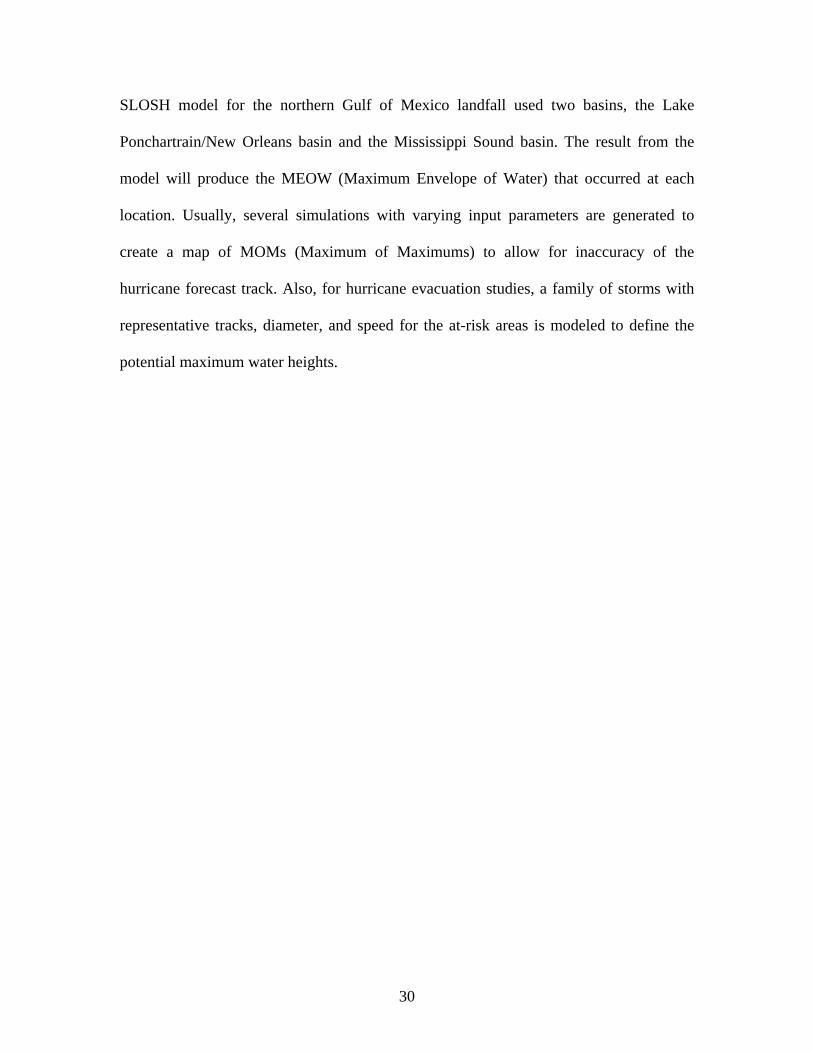
3.2 Floodplain Mesh Development
For storm surge simulations expected to produce water flooding over inland areas,
complex coastal and inland geometry, as well as bathymetry must be well represented. In
this study, modifications to the preliminary in-bank mesh concerning the Lower
Pascagoula and Escatawpa Region have been completed by generating additional
computational regions inland, where much of the marsh region is inundated during storm
surge events (Figure 3.3). SMS 9.2 is utilized throughout the mesh development process
employed herein.
Figure 3.3 Figure 3.4 Satellite Images of Marsh Areas in the Lower Pascagoula and Escatawpa Rivers (image courtesy of Google Earth)
36
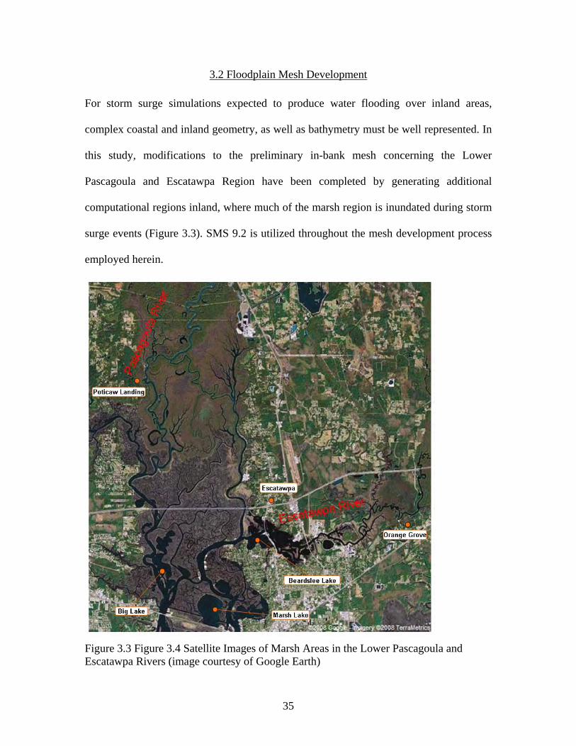
An initial development of the floodplain model employs topography up to the 1.5-meter
contour, where all topography data used in the floodplain mesh originates from the SL15
mesh (Figure 3.4). One target of this model is improve upon the tide-only model results
presented by Wang (2008), which implied the necessity to include the marsh areas in
order to sufficiently describe tide-driven flows within the river bank. The resolution of
the marsh area is based on that used by the SL15 mesh. Bathymetry within the
preliminary in-bank mesh remains from that of Wang (2008), and the bathymetry within
the additional inland area and refined transition area has been interpolated from the SL15
mesh. With this initial version of the floodplain model (herein referred to as
FP1.5_INLET_A; Figure 3.5, Figure 3.6), it will be demonstrated in Chapter 6 that the
floodplain mesh provides for an improved result with respect to the astronomic tide
solution in the Pascagoula River.
Figure 3.5 SL15 Mesh: Topography Contours Up to 1.5 m above NAVD88

37
Figure 3.6 Inlet-based 1.5 m Floodplain Mesh (FP1.5_INLET_A; Used for Astronomic Tide Simulation)

38
Figure 3.7 Inlet-based 1.5 m Floodplain Mesh (FP1.5_INLET_A; Typically for Astronomic Tide Simulation)

39
However, in order to simulate storm surge events, it is necessary for some river islands
located at and near the inlets within the floodplain area be meshed over to allow for the
wetting/drying of elements. Four islands within the FP1.5_INLET_A mesh were meshed
over using SMS with the respective topography interpolated from the SL15 mesh. The
resulting mesh consists of 112,451 computational nodes and 217,358 triangular elements
(FP1.5_INLET_B; Figure 3.7).
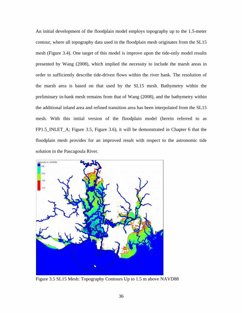
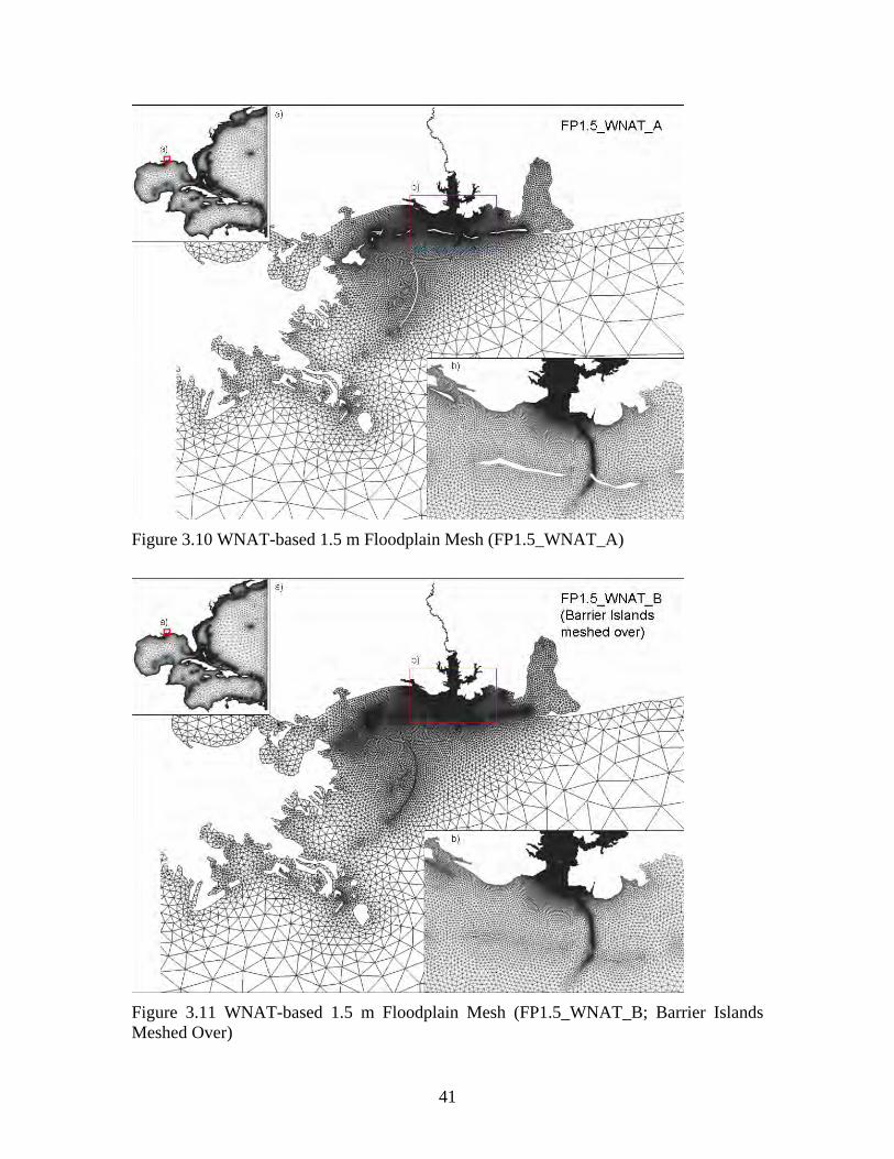
Next, the 1.5-m floodplain mesh was incorporated into the WNAT-53K model domain
(Figure 1.2). The coastline and barrier island boundaries are refined by digitized shoreline
data retrieved from the Coastline Extractor (National Geophysical Data Center [NGDC]).
Approximately 160 km of coastline from Waveland, Mississippi (just west of St. Louis
Bay) at the west to Gulf Shores, Alabama (just east of Mobile Bay) at the east is selected
since it is expected to influence the storm surge dynamics in the Pascagoula River during
a hurricane event (Figure 3.8). Furthermore, it was necessary to reconstruct the mesh
region within 80 km of the Pascagoula Inlet in order to obtain a reasonably smooth
transition between the local (1.5-m floodplain) and the global (WNAT-53K) mesh
boundaries. It is noted that the mesh resolution at the shipping channel through one of
barrier islands (Petit Bois Island) is increased to capture the deeper bathymetry. For
barrier islands, we have obtained two variations; one has a no-flow boundary and values
at the boundary nodes are adjusted to 0.5 m (FP1.5_WNAT_A; Figure 3.9), while the
other has meshed over islands and its topography is directly interpolated from the SL15
mesh (FP1.5_WNAT_B; Figure 3.10). Table 3.1 present a summary of the mesh
variations.

40
Figure 3.8 Inlet-based 1.5 m Floodplain Mesh (FP1.5_INLET_B; River Islands Meshed Over)
Figure 3.9 Coastline Boundary Comparisons
41
Figure 3.10 WNAT-based 1.5 m Floodplain Mesh (FP1.5_WNAT_A)
Figure 3.11 WNAT-based 1.5 m Floodplain Mesh (FP1.5_WNAT_B; Barrier Islands Meshed Over)
42
Table 3.1 Summary of Mesh Variations

43
CHAPTER 4. MODEL DESCRIPTION
This chapter represents a description of the numerical code, ADCIRC-2DDI (Advanced
Circulation Two-dimensional Depth-integrated software) along with the following two
topics: 1) hydrodynamic model, 2) tropical wind stress and pressure field.
4.1 Hydrodynamic Model
To compute the water-surface elevations and currents during Hurricane Katrina,
ADCIRC-2DDI, a finite element hydrodynamic model which solves the nonlinear
shallow water equations, is applied to the shallow-water river and estuarine systems
concerning the Pascagoula River.
The depth integrated equations of mass and momentum conservation are used in
ADCIRC-2DDI, subject to the incompressibility, Boussinesq, and hydrostatic pressure
approximations. In a spherical coordinate system, the following equations are set up: the
continuity equation (4.1) and momentum equations (4.2) and (4.3).
( ) 0coscos1
=⎥⎦
⎤⎢⎣
⎡∂
∂+
∂∂
+∂∂
φφ
λφζ VHUH
Rt (4.1)
( ) UHp
gpp
R
VfUR
UVR
UUR
UtU
ss*
00cos1
tan1cos
ττ
ηζλφ
φφλφ
λ −+⎥⎦
⎤⎢⎣
⎡−+
∂∂
−=
⎟⎠⎞
⎜⎝⎛ +−
∂∂
+∂∂
+∂∂
(4.2)

44
( ) UHp
gpp
R
UfUR
VVR
UUR
UtV
ss*
00
1
tan1cos
ττ
ηζφ
φφλφ
φ −+⎥⎦
⎤⎢⎣
⎡−+
∂∂
−=
⎟⎠⎞
⎜⎝⎛ +−
∂∂
+∂∂
+∂∂
(4.3)
where
t = time
λφ , = degrees longitude and degrees latitude
ζ = free surface elevation
VU , = depth-averaged horizontal velocities in the λ and φ directions
R = radius of the Earth,
hH += ζ = total height of the water column
h = bathymetric depth
φsin2Ω=f = Coriolis parameter
Ω = angular speed of the Earth
sp = atmospheric pressure at the free surface
g = acceleration due to gravity
η = effective Newtonian equilibrium tide potential
0p = reference density of water
φλ ττ ss , = applied free surface stresses (e.g., wind and wave radiation stresses)
( )H
VUC f
22
*+
=τ = bottom stress

45
fC = bottom friction coefficient
In these governing equations of the hydrodynamic model, continuity (see Eq. (4.1))
provides a balance between the water level and the flux into/out of the water column.
Momentum (see Eqs. (4.2) and (4.3)) provides a balance between the location
acceleration (left-most term) and the following effects (given in the order as presented in
Eqs. (4.1) and (4.2)): 2) advection; 3) Coriolis; 4) atmospheric pressure; 5) pressure; 6)
tidal potential; 7) surface wind stress; 8) bottom friction.
The effective expression for the effective Newtonian equilibrium tide potential is given
by Reid (1990) as:
( ) ( ) ( ) ( )( )⎥
⎥⎦
⎤
⎢⎢⎣
⎡
++−
= ∑0
0
,0
2cos,,
tvjTtt
LtfCtjnjnjn
jjnjnjn λπ
φαφλη (4.4)
where
jnC = constant characterizing the amplitude of tidal constituent n of species j
jnα = effective earth elasticity factor for tidal constituent n of species j
jnf = time-dependent nodal factor
jnv = time-dependent astronomical argument
j = 0, 1, 2 = tidal species (0: declinational; 1: diurnal; 2: semidiurnal)
1sin3 20 −= φL
( )φ2sin1 =L
( )φ22 cos=L

46
φλ , = degrees longitude and degrees latitude
0t = reference time
jnT = period of constituent n of species j
Reid (1990) suggests typical values for jnC , and a value of 0.69 is suggested for the
effective earth elasticity factor α for all the tidal constituents, although it has been proven
to be slightly constituent dependent (Schwiderski, 1980; Hendershott, 1981; Wahr, 1981).
Equations (4.1) to (4.3) are transformed from spherical into Cartesian coordinate system
using a Carte Parallelo-grammatique cylindrical map projection (CPP) as part of the
solution procedure (Westerink 1994):
( ) 00 cos' φλλ −= Rx (4.5)
φRy =' (4.6)
where
00 ,φλ = center point of the projection
Applying the CPP, (4.5) and (4.6), to the original fully nonlinear shallow water equations,
(4.1) to (4.3), leads to the primitive nonconservative expressions in a CPP coordinate
system:
( ) ( ) 0'
coscos
1'cos
cos 0 =∂
∂+
∂∂
+∂∂
yVH
xUH
Rtφ
φφφζ (4.7)
47
( ) UH
gp
x
VfURy
UVxUU
tU
ss*
00
0
0
'coscos
tan''cos
cos
τρτ
ηζρφ
φ
φφφ
λ −+⎥⎦
⎤⎢⎣
⎡−+
∂∂
−=
⎟⎠⎞
⎜⎝⎛ +−
∂∂
+∂∂
+∂∂
(4.8)
( ) VH
gp
y
UfURy
VVxVU
tV
ss*
00
0
'
tan''cos
cos
τρτ
ηζρ
φφφ
φ −+⎥⎦
⎤⎢⎣
⎡−+
∂∂
−=
⎟⎠⎞
⎜⎝⎛ +−
∂∂
+∂∂
+∂∂
(4.9)
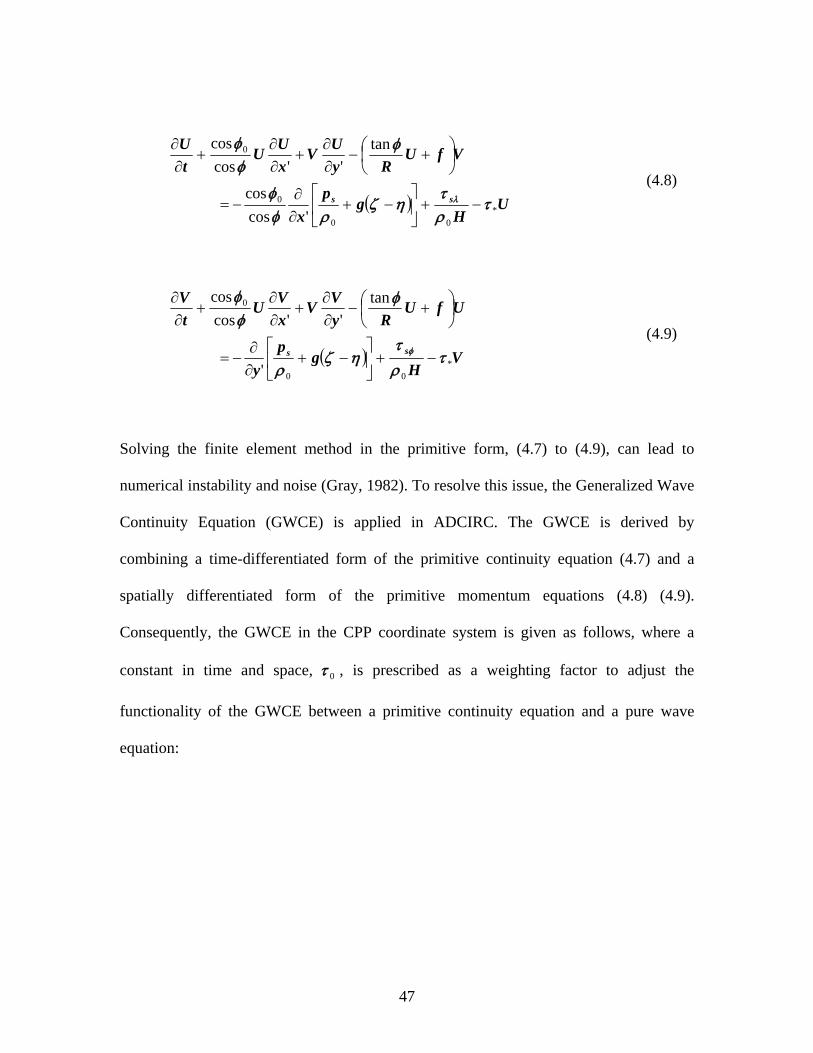
Solving the finite element method in the primitive form, (4.7) to (4.9), can lead to
numerical instability and noise (Gray, 1982). To resolve this issue, the Generalized Wave
Continuity Equation (GWCE) is applied in ADCIRC. The GWCE is derived by
combining a time-differentiated form of the primitive continuity equation (4.7) and a
spatially differentiated form of the primitive momentum equations (4.8) (4.9).
Consequently, the GWCE in the CPP coordinate system is given as follows, where a
constant in time and space, 0τ , is prescribed as a weighting factor to adjust the
functionality of the GWCE between a primitive continuity equation and a pure wave
equation:

48
( ) ( )
( ) ( )
0
tantan
'
tan''cos
cos'
'coscos
tan''cos
cos'cos
cos
0
00*
0
0
00*
0
0
00
02
2
=
⎟⎠⎞
⎜⎝⎛−⎟
⎠⎞
⎜⎝⎛
∂∂
−
⎭⎬⎫
+−−⎥⎦
⎤⎢⎣
⎡−+
∂∂
−
⎩⎨⎧
⎟⎠⎞
⎜⎝⎛ +−
∂∂
−∂∂
−∂∂
∂∂
+
⎭⎬⎫
+−−⎥⎦
⎤⎢⎣
⎡−+
∂∂
−
⎩⎨⎧
⎟⎠⎞
⎜⎝⎛ ++
∂∂
−∂∂
−∂∂
∂∂
+
∂∂
+∂∂
VHR
VHRt
VHgp
yH
UHfURy
VVHxvUH
tV
y
UHgp
xH
VHfURy
UVHxUUHU
tx
tt
ss
ss
φτφ
ρτ
ττηζρ
φφφζ
ρτ
ττηζρφ
φ
φφφζ
φφ
ζτζ
φ
λ
(4.10)
This study applies the hybrid bottom friction function which is more accurate in shallow
water. The quadratic bottom friction equation that is used with the hybrid bottom friction
formulation is defined ∗τ = bottom stress as:
( )H
VUC f2122 +
=∗τ (4.11)
where
Cf = bottom friction factor
with the hybrid bottom friction, the bottom friction coefficient is defined as:
θλ
θ
⎥⎥⎦
⎤
⎢⎢⎣
⎡⎟⎠⎞
⎜⎝⎛+=
HH
CC breakff 1
min (4.12)

49
where
minfC = minimum friction factor that is approached in deep water when the hybrid
bottom friction function reverts to the quadratic bottom friction function
breakH = break depth to determine if hybrid function will act like a quadratic
function or increase with depth similar to a Manning’s type friction
θ = dimensionless parameter that determines how rapidly the hybrid function
approaches its upper and lower limits
λ = dimensionless parameter that describes how quickly the friction factor
increases as water depth decreases
As bathymetric depth approaches zero, the friction factor becomesλ
⎟⎠⎞
⎜⎝⎛
HH
C breakfmin
. Also,
as the depth approaches infinity, the friction factor approachesminfC .
Wang (2008) calibrated spatially varied minfC values throughout the Pascagoula region
and concluded that 0.0025(ocean region)-0.0075(marsh area)-0.0055(middle stream &
upstream) is suggested as a good starting point with respect to astronomic tide
simulation; however, in this study a value of 0.0025 is used as the standard value
(Luettich et al., 1992).

50
4.2 Tropical Wind Stress and Pressure Field
The lower layer of the troposphere where continuous turbulent processes occur is known
as the planetary boundary layer (PBL), while the upper layer is known as the free
atmosphere since there are no frictional influences (Figure ?4.1). The thickness of PBL is
about 1 to 2 km but varies diurnally depending on the energy budget between the land
surface and the upper layer, which is affected by variable parameters such as heat,
moisture, buoyancy, wind shear, and surface roughness. Wind is turbulent and gusty
within the PBL, and the surface friction causes eddies and develops chaotic wind patterns.
Most of the relevant weather and climate phenomena, including hurricanes, we
experience on the Earth are driven by changes of the physical and chemical conditions
within the PBL; therefore, it is necessary to translate these meteorological features into a
forcing mechanism that can be incorporated into the numerical model in order to
accomplish an accurate forecasting system.
Figure 4.1 Planetary Boundary Layer (http://www.shodor.org)
Chow’s vortex model (1971) was primarily introduced as a theoretical basis of the
numerical schemes used to solve the primitive equations on a high resolution and

51
considered the asymmetry airflow in the PBL, which is important since the frictionally
induced convergence in the layer leads to moist convection and ultimately produces the
instability responsible for the development of tropical cyclones. The model is termed by
the equation of horizontal motion, vertically averaged through the depth of the PBL in
coordinates fixed to the Earth:
VVh
CVKPVkf
dtdV D
H ⎟⎠
⎞⎜⎝
⎛−+∇⋅∇+⎟⎟⎠
⎞⎜⎜⎝
⎛∇−=×+
ρ1ˆ (4.13)
where
∇⋅+∂∂
= Vtdt
dV
t∂∂ = local time change relative to fixed coordinates
∇ = two-dimensional del operator
V = vertically averaged horizontal wind velocity
f = Coriolis parameter
k̂ = unit vector in the vertical direction
airρ = mean air density
P = depth-averaged pressure in the PBL
H = horizontal eddy viscosity coefficient
DC = surface drag coefficient
h = depth of the PBL

52
These approximations consider that the vertical advection of momentum is small enough
to be neglected compared to the horizontal advection and that the shear stress at the top of
the PBL is assumed to be zero.
The total pressure P is defined as PPP c += (4.14)
where
cP = pressure field associated with the tropical cyclone translating with the storm
at a speed cV
P = large scale pressure field which is given by the corresponding constant
geostrophic velocity gV as:
⎟⎟⎠
⎞⎜⎜⎝
⎛∇−=× PVkf g ρ
1ˆ (4.15)
Substituting these pressure specification equations (4.14) and (4.15) into (4.13) yields
( ) VVh
CVKPVVkfdtdV D
Hcg ⎟⎠⎞
⎜⎝⎛−+∇⋅∇+⎟⎟
⎠
⎞⎜⎜⎝
⎛∇−=−×+
ρ1ˆ (4.16)
The governing equations used in the model are formed with respect to a moving
Cartesian coordinate system ( )yx, whose origin is located at the low pressure center of
the storm (storm’s eye).
It is also noted that the pressure field cP is radially symmetric and prescribed by the well-
known exponential pressure law:

53
( )rRc pePP /
0−Δ+= (4.17)
where
0P = pressure at the center of the storm
0PPp −=Δ = pressure anomaly
R = scale radius ≈ radius to the maximum wind
r = radial distance from the center
With an option specifying pΔ and R by storm quadrant, an asymmetrical pressure field
results after smoothing between the pressure variations specified for each quadrant.
ADCIRC incorporates the PBL model that has been modified to directly interface.
Internally, ADCIRC applies the Garratt (1977) formulation to convert the wind velocities
that is computed over the nested grid of the PBL model to wind stress:
xair
Dx WWC
00 ρρ
ρτ
= (4.18)
and
yair
Dy WWC
00 ρρ
ρτ
= (4.19)
where
yx ττ , = wind stress in the x and y directions
0ρρ air = ratio of sir density to average density of seawater, 0.001293
( ) 001.0067.075.0 WC D += = frictional drag coefficient W = magnitude of wind velocity

54
yx WW , = components of the wind velocity vector in the x and y directions
The PBL model does not compute pressure but rather determines the pressure gradient,
however, ADCIRC requires a pressure file expressed as an equivalent height of water
( )gP wρ/ as an input; therefore the PBL model has been modified to provide hourly wind
stress and ( )gP wρ/ values, where all data are linearly interpolated onto all nodal points
in the finite element computational grid used by ADCIRC.

55
CHAPTER 5. MODEL SETUP
This chapter presents the model setup used in ADCIRC simulations. First, the forcings
assigned to the open-ocean boundary and each computational nodal point over the mesh
are discussed. In this study, 1) astronomic tides, 2) winds and pressures, and 3) storm
surge hydrographs are prescribed individually or collectively. Next, the model parameters
involved in the simulations, such as bottom friction and wetting and drying, are
introduced. These model settings remain constant in all simulations (except when noted
in Table 5.2).
5.1 Model Forcings
5.1.1 Astronomic Tides
Astronomic tides are the cyclical rise and fall of the ocean water level due to earth’s
gravitational interaction with the moon and sun. Tides are periodic in nature primarily
due to the cyclical influence of the Earth's rotation and may be semidiurnal (two high
waters and two low waters each day) or diurnal (one tidal cycle per day). In most
locations along the coastline, the tides are semidiurnal; however, throughout much of the
Gulf of Mexico, the tides are diurnal in their behavior. A tidal analysis is a linear
regression of a sea level time series in terms of harmonic tidal constituents which can be
represented as a superposition of multiple sinusoids. The amplitudes and phase lags for
each tidal constituent are determined from the harmonic analysis.

56
For the WNAT-based models involving the Western North Atlantic, an open-ocean
boundary at the 60 degree West meridian is assigned and forced with seven tidal forcings
(K1, O1, M2, S2, N2, K2, Q1; Table 5.1) These same constituents are applied over the
interior of the computational domain in the form of tidal potentials (Reid, 1990).
Table 5.1 Seven tidal constituents used to force the WNAT-based model
Constituent Name Period (hr) Frequency (rad/s) K1 Luni-solar diurnal 23.93 0.000072921158358 O1 Principal Lunar Diurnal 25.82 0.000067597744151 M2 Principal Lunar Semidiurnal 12.42 0.000140518902509 S2 Principal Solar Semidiurnal 12.00 0.000145444104333 N2 Larger Lunar Elliptic 12.66 0.000137879699487 K2 Luni-solar Semidiurnal 11.97 0.000145842317201 Q1 Larger Lunar Elliptic Diurnal 26.87 0.000064958541129
For the localized (i.e. inlet-based) model, an open-ocean boundary is assigned at the
semi-circular boundary and forced with twenty-three tidal constituents (STEADY, MN4,
SM, O1, K1, MNS2, 2MS2, N2, M2, 2MN2, S2, 2SM2, MN4, M4, MS4, 2MN6, M6,
MSN6, M8, M10, P1, K2, and Q1; APPENDIX C). No tidal potential forcings are
applied over the interior of the computational domain due to the local extent of the inlet-
based mesh (Reid, 1990). Amplitudes and phases associated with the twenty-three tidal
constituents listed in Appendix C are generated for the open-ocean boundaries of the
localized domains, based on a harmonic analysis of a tide-driven simulation using the
WNAT-based model domain.

57
5.1.2 Wind and Pressure
Storm surge is mainly driven by the sustained winds acting during a storm event. Further,
due to the decreasing bathymetry as the coast is approached, storm surge can accumulate
greatly in shallow coastal regions. It is evident that the meteorological influence caused
by local winds and pressures should be included in a storm surge model.
Wind and pressure field data associated with Hurricane Katrina (for the dates August 23
to 30, 2005) (provided by Oceanweather Inc.) is incorporated into the numerical model.
The provided data are 30-minute-sustained meteorological effects and are calculated by a
tropical wind field model (TC96, Thompson and Cardone, 1996) governed by vertically
averaged equations of motion that describe horizontal airflow through the planetary
boundary layer. It is assumed that the structure of the tropical cyclone changes relatively
slowly over time. TC96 calculates “snapshots” (in time) that represent distinct phases of
the storm’s evolution. In order to determine a circularly symmetric pressure field
centered at the eye of the storm, an exponential pressure law is employed (Holland, 1980).
The extent of the wind and pressure field data coverage is shown in Figure 5.1, where it
covers the WNAT-53K model domain in its entirety.
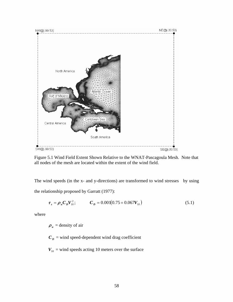
58
Figure 5.1 Wind Field Extent Shown Relative to the WNAT-Pascagoula Mesh. Note that all nodes of the mesh are located within the extent of the wind field.
The wind speeds (in the x- and y-directions) are transformed to wind stresses by using
the relationship proposed by Garratt (1977):
210VC Dus ρτ = ; ( )10067.075.0001.0 VC D += (5.1)
where
uρ = density of air
DC = wind speed-dependent wind drag coefficient
10V = wind speeds acting 10 meters over the surface

59
The computed wind stresses are interpolated to the nodes of the mesh using a linear
interpolation scheme. In order to transform the atmospheric pressures (in stress units)
into equivalent water heights ηp , an inverted barometer effect is applied:
gp
pwρσ
η = (5.2)
where
wρ = density of seawater
g = acceleration due to gravity
In the resulting file, a Single Meteorological Input File (fort.22, APPENDIX D), wind
stresses and atmospheric pressures during Hurricane Katrina are specified at all grid
nodes associated with the ADCIRC Grid and Boundary Information File (fort.14). Figure
5.2 and Figure 5.3 show the direction and magnitude of the wind speed associated with
Hurricane Katrina at 02:30 GMT on August 29, 2005. The meteorological forcing data in
fort.22 is read into the simulation every 30 minutes over the 7 day simulation period
(August 23, 2005, 0:00 GMT to August 30, 0:00 GMT). Other principal parameters
specified in the Model Parameter and Periodic Boundary Condition File (fort.15) are
discussed in the following Section 5.2. Note that the open-ocean boundary specified in
fort.14 must be changed to a land (no-flow) boundary if winds and pressures are used
alone as boundary conditions.
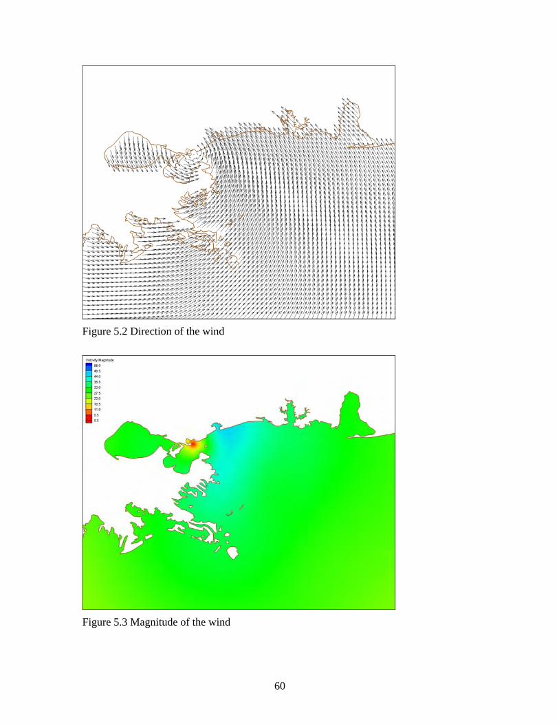
60
Figure 5.2 Direction of the wind
Figure 5.3 Magnitude of the wind

61
5.1.3 Storm Surge Hydrograph
A large-scale modeling approach that describes the hydrodynamics from the deep ocean
into the local estuary ensures an adequate description of the storm surge dynamics
(Bacopoulos et al., 2008); however, in order to increase computational efficiency while
maintaining this level of accuracy, a localized domain (e.g. an inlet-based model) is
selected as the operational storm surge model. Instead of applying wind and pressure data
directly into the localized domain, the storm surge hydrograph approach allows for time
varying elevation boundary conditions which are read from an input file (Non-periodic
Elevation Boundary Condition File, fort.19). The elevation forcing data at specified
nodes and incremental time step are described in the fort.19.
In order to obtain the elevation boundary conditions (fort.19) at the various open-ocean
boundaries of the localized domains, Hurricane Katrina’s wind and pressure data
described in the previous section are applied to the WNAT-53K model domain. In this
simulation, the open-ocean boundary of the localized mesh domain is specified as output
locations for the generation of the storm surge hydrograph (Model Parameter and
Periodic Boundary Condition File, fort.15). As a result, the elevation time series at the
specified boundary output (fort.61) is obtained and used as an input forcing for the
localized domain (fort.19). The calculated storm surge hydrographs that are applied to the
open-ocean boundaries of the localized model domains are presented in Chapter 6.

62
5.2 Model Parameters
The following model parameterizations are set up in the Model Parameter and Periodic
Boundary Condition File (fort.15): simulations are begun from a cold start; the wetting
and drying algorithm is enabled with the minimum bathymetric depth set to 0.1 m. (i.e.
computational nodes and the accompanying elements with water depths less than the
prescribed minimum bathymetric depth are considered to be dry); the hybrid bottom
friction formulation is employed varying the minimum bottom friction factor according
to the simulation results that follow and specifying the remaining hybrid bottom friction
parameter values as determined by Hagen et al. (2005a): mHbreak 0.1= , 10=θ , and
31
=λ ; and the horizontal eddy viscosity is set to 2/0.5 sm . Other principal parameters
which vary depending on model domain and forcings are tabulated in Table 5.2. For the
localized domains, a Cartesian coordinate system is used; the simulation period is 90 days
for the astronomic tides and 7 days for Hurricane Katrina (e.g. winds and pressures
and/or storm surge hydrographs) with 20- and 0.5-day ramping periods, respectively; the
advection terms are turned off for the WNAT-based models and all Hurricane Katrina
runs since the resulting velocities are not evaluated in this study. A computational time
step is specified for each simulation to ensure that the Courant number criterion is
satisfied throughout the computational domain.
0.1# ≤⎟⎠⎞
⎜⎝⎛ΔΔ
=xtghC
where
#C = Courant number

63
g = gravity acceleration
h = bathymetric depth
tΔ = applied computational time step
xΔ = nodal spacing
A zero-flux boundary condition (similar to infinite vertical walls) is applied to mainland
coastlines and island shorelines and specified in the ADCIRC Grid and Boundary
Information File (fort.14).

64
Table 5.2 Model Parameters
( 0τ is the GWCE weighting parameter.)

65
CHAPTER 6. MODEL RESULTS
This chapter presents the ADCIRC model results. Table 6.1 shows a summary of the
simulations conducted in this study. First, the inlet-based floodplain meshes
(FP1.5_INLET_A and FP1.5_INLET_B in Table 3.1) are each applied in a tidal
simulation (Experiments No.1 and No.2). The floodplain (tide-only) model results are
compared with the preliminary in-bank (tide-only) model results to observe the effect of
the inundation areas on tidal elevations in the Pascagoula River. Next, Experiments No.3
and No.4 apply winds and pressures over the WNAT-53K and FP1.5_WNAT_B model
domains, respectively. Products of Experiments No.3 and No.4 will be storm surge
hydrographs which will be used as boundary forcings for the inlet-based model
applications performed in Experiments No.5, No.6, and No.7. Experiment No.5 examines
the inlet-based 1.5-m floodplain model (FP1.5_INLET_B in Table 3.1) that is forced by
storm surge hydrograph provided by using the WNAT-53K mesh domain at the open-
ocean boundary. Next, the storm surge hydrographs produced from Experiment No.4 are
applied on the inlet-based model: Experiment No.6 uses a hydrograph only; Experiment
No.7 uses the hydrograph in combination with a local wind and pressure forcing.
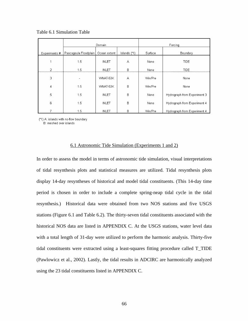
66
Table 6.1 Simulation Table
6.1 Astronomic Tide Simulation (Experiments 1 and 2)
In order to assess the model in terms of astronomic tide simulation, visual interpretations
of tidal resynthesis plots and statistical measures are utilized. Tidal resynthesis plots
display 14-day resyntheses of historical and model tidal constituents. (This 14-day time
period is chosen in order to include a complete spring-neap tidal cycle in the tidal
resynthesis.) Historical data were obtained from two NOS stations and five USGS
stations (Figure 6.1 and Table 6.2). The thirty-seven tidal constituents associated with the
historical NOS data are listed in APPENDIX C. At the USGS stations, water level data
with a total length of 31-day were utilized to perform the harmonic analysis. Thirty-five
tidal constituents were extracted using a least-squares fitting procedure called T_TIDE
(Pawlowicz et al., 2002). Lastly, the tidal results in ADCIRC are harmonically analyzed
using the 23 tidal constituents listed in APPENDIX C.

67
Each tidal signal is resynthesized through the following summation:
( )[ ]nnnnnnN
uVgtfHZzT ++−+= ∑ ωcos)( 0
where
0Z = local mean sea level (MSL)
),( nn gH = (tidal constituent amplitude and phase)
Also, the nodal adjustment factors are given as nf and nu and the terms tnω and
nV together determine the phase angle of the equilibrium tidal constituent. nV is the
equilibrium phase angle for the tidal constituent at the arbitrary time origin. The accepted
convention is to take nV as the Prime Meridian and t in the standard time zone of the
observation station.

68
Figure 6.1 Historical Data Stations Table 6.2 Historical Data Stations
Wang (2008) has suggested that incorporating the marsh areas into the preliminary in-
bank mesh may yield more accurate results in the tidal resynthesis; therefore, this section
demonstrates an improved inlet-based astronomic tide model for the Pascagoula River
using floodplain meshes, FP1.5_INLET_A and FP1.5_INLET_B (Figure 3.6 to Figure
69
3.8). Recall that the FP1.5_INLET_A mesh describes river islands as no-flow boundaries
while the FP1.5_INLET_B mesh describes river islands with elements that are allowed to
wet and dry.
Figure 6.2 to Figure 6.5 show resynthesized plots at the seven recording stations based on
the model output from Experiments 1 and 2. The first four stations (shown in Figure 6.2
and Figure 6.3) reveal little difference for when the inundation areas are included in the
model domain. (We note that for station No.1 at Pascagoula, MS, no model result is
provided for the FP1.5_INLET_B mesh application since the location dries out during the
simulation.) While there is a slight improvement in the model result at Station No.4
(Gautier, MS) (see Figure 6.3), we conclude that tidal elevations near the coast are
dominated by the deep-ocean tide and are weakly influenced by the inundation areas. On
the other hand, the upstream locations (Station Nos. 5-7) are shown to be strongly
influenced by the inundation areas (see Figure 6.4 and Figure 6.5). There is a significant
reduction in the modeled tidal amplitude, which can be explained by the wetting and
drying that is occurring in the floodplains. The wetting and drying of the inundation areas
also appears to have an effect on the phase of the tide in the upstream regions of the
Pascagoula River. Not only do the marsh areas of the Lower Pascagoula River need be
included in the computational domain (see modeled tide results for Stations 5 and 6 in
Figure 6.4), but the inundation areas lying adjacent to the Escatawpa River need be
considered (see modeled tide results for Station 7 in Figure 6.5).
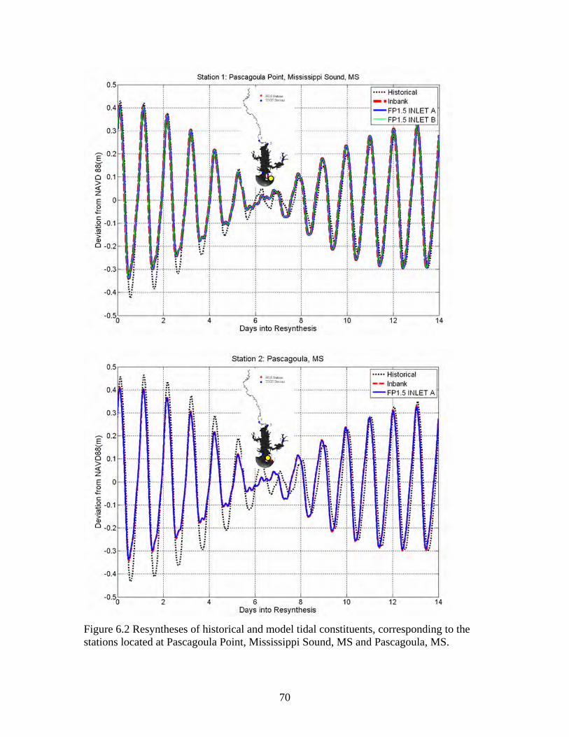
70
Figure 6.2 Resyntheses of historical and model tidal constituents, corresponding to the stations located at Pascagoula Point, Mississippi Sound, MS and Pascagoula, MS.

71
Figure 6.3 Resyntheses of historical and model tidal constituents, corresponding to the stations located at Pascagoula River Mile 1, MS and West Pascagoula at Gautier, MS.

72
Figure 6.4 Resyntheses of historical and model tidal constituents, corresponding to the stations at Pascagoula River at Cumbest Bluff and Graham Ferry, MS.

73
Figure 6.5 Resyntheses of historical and model tidal constituents, corresponding to the station located at Escatawpa River at I-10 near Orange Grove, MS.

74
6.2 Storm Surge Model
6.2.1 WNAT-based Model and Storm Surge Hygrograph Extraction (Experiments 3 and
4)
In order to obtain storm surge hydrographs (elevation variance) at the open-ocean
boundary locations associated with the localized domain, a large-scale modeling
approach will utilize high-resolution wind and pressure fields of Hurricane Katrina. First,
Experiment 3 applies winds and pressures over the WNAT-53K model domain to
produce results (storm surge hydrographs) at the ninety-nine open-ocean boundary nodes
of inlet-based mesh (Figure 6.6). Then Experiment 4 applies winds and pressures over the
WNAT-based Pascagoula floodplain mesh (FP1.5_WNAT). It should be noted that the
WNAT-53K mesh contains a coarse discretizations of the Gulf Coast with Mississippi
barrier islands assigned as no-flow boundaries while the FP1.5_WNAT mesh employs a
refined coastline and meshes over barrier islands to allow for storm surge overtop.
Figure 6.7 to Figure 6.17 show calculated storm surge hydrographs at ten (of the ninety-
nine) boundary nodes by both Experiments 3 and 4. Since the landfall position of
Hurricane Katrina located west of the study area, the modeled surge height is the highest
at the position 1, which is about 3.5 m (Figure 6.7). Then the modeled height of the storm
surge gradually decreases as one progresses eastward on the open-ocean boundary (i.e.
from number 1 to 99). Each result shows that the modeled surge level of the WNAT-53K
model domain (in red line) is higher than the model surge level produced by the
FP1.5_WNAT mesh (in blue dashed line). In fact, for the greatest storm surge height on
the westernmost point of the open-ocean boundary, the WNAT-53K mesh can over-

75
predict the water level (relative to that produced by the FP1.5_WNAT mesh) by nearly as
much as 0.5 meter. There are multiple suggestions for the significant differences in the
storm surge hydrographs presented in Figure 6.7 to Figure 6.17. First, the FP1.5_WNAT
mesh contains a high-resolution description of the inland waterbody and floodplain
features of the Pascagoula River, where the WNAT-53K mesh does not include the
estuary. Second, the coastline boundary of the FP1.5_WNAT mesh has been refined to
more closely follow the true coastline, where the WNAT-53K mesh utilizes a coarse
resolution that does not sufficiently capture the intricate coastline geometry. The barrier
islands protecting the Pascagoula River are described as no-flow boundaries in the
WNAT-53K mesh. Meshing over the barrier islands in the FP1.5_WNAT mesh permits
for the storm surge to overtop the barrier islands. It is argued that the no-flow boundaries
used by the WNAT-53K mesh allows for the storm surge to accumulate to greater heights
because the flow is more confined by the no-flow boundaries, whereas the FP1.5_WNAT
mesh permits for the storm surge to propagate over the barrier islands and into the estuary
(Salisbury and Hagen, 2007).
Figure 6.7 to Figure 6.17 show calculated storm surge hydrographs at ten boundary nodes
by both Experiments. Since the landfall position of Hurricane Katrina located west of the
study area, the modeled surge height is the highest at the position 1, which is about 3.5 m
(Figure 6.7). Then the modeled height of the storm surge gradually decreases toward east
(i.e. number 1 to 99). Each result shows the modeled surge level of 53K domain (in red
line) is higher than the level of FP1.5_WNAT (in blue dash line). The difference is
caused by: 1) entire mesh resolution: FP1.5_WNAT, a high-resolution flood plain mesh,
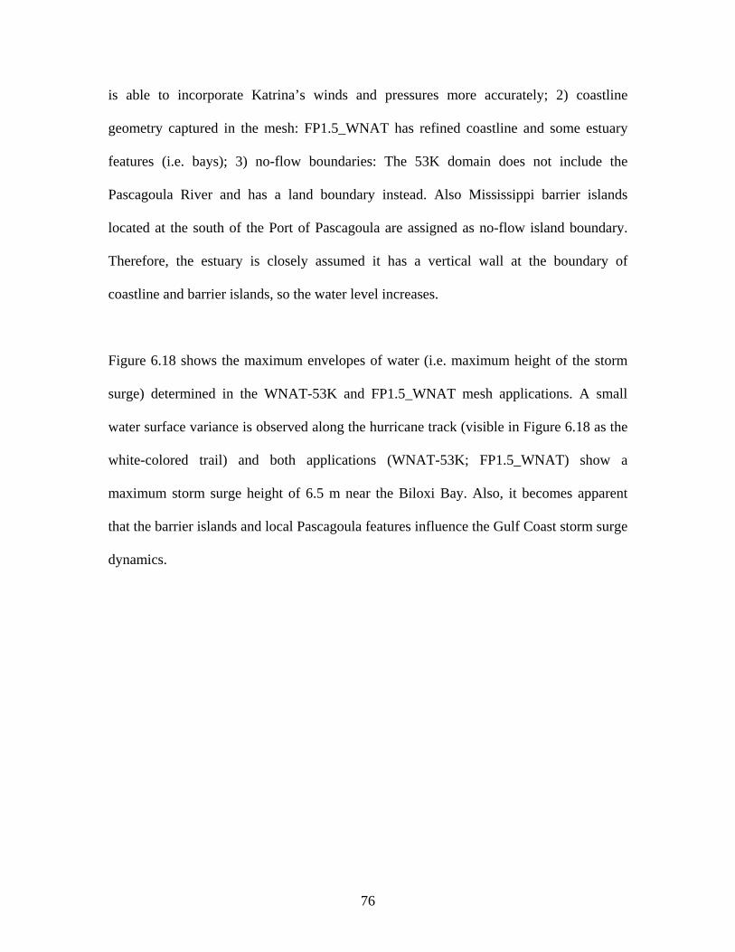
76
is able to incorporate Katrina’s winds and pressures more accurately; 2) coastline
geometry captured in the mesh: FP1.5_WNAT has refined coastline and some estuary
features (i.e. bays); 3) no-flow boundaries: The 53K domain does not include the
Pascagoula River and has a land boundary instead. Also Mississippi barrier islands
located at the south of the Port of Pascagoula are assigned as no-flow island boundary.
Therefore, the estuary is closely assumed it has a vertical wall at the boundary of
coastline and barrier islands, so the water level increases.
Figure 6.18 shows the maximum envelopes of water (i.e. maximum height of the storm
surge) determined in the WNAT-53K and FP1.5_WNAT mesh applications. A small
water surface variance is observed along the hurricane track (visible in Figure 6.18 as the
white-colored trail) and both applications (WNAT-53K; FP1.5_WNAT) show a
maximum storm surge height of 6.5 m near the Biloxi Bay. Also, it becomes apparent
that the barrier islands and local Pascagoula features influence the Gulf Coast storm surge
dynamics.

77
Figure 6.6 Ninety-nine Open Ocean Boundary Nodes of FP1.5_INLET Model
Figure 6.7 Storm Surge Hydrograph at Open-ocean Boundary Node 1

78
Figure 6.8 Storm Surge Hydrograph at Open-ocean Boundary Node 10
Figure 6.9 Storm Surge Hydrograph at Open-ocean Boundary Node 20

79
Figure 6.10 Storm Surge Hydrograph at Open-ocean Boundary Node 30
Figure 6.11 Storm Surge Hydrograph at Open-ocean Boundary Node 40

80
Figure 6.12 Storm Surge Hydrograph at Open-ocean Boundary Node 50
Figure 6.13 Storm Surge Hydrograph at Open-ocean Boundary Node 60

81
Figure 6.14 Storm Surge Hydrograph at Open-ocean Boundary Node 70
Figure 6.15 Storm Surge Hydrograph at Open-ocean Boundary Node 80

82
Figure 6.16 Storm Surge Hydrograph at Open-ocean Boundary Node 90
Figure 6.17 Storm Surge Hydrograph at Open-ocean Boundary Node 99

83
Figure 6.18 Maximum Envelop of Water (Top) FP1.5_WNAT model forced by global wind and pressure; (Middle left& right) Insets of Gulf Coast in 53K and FP1.5_WNAT model; (Bottom left& right) Insets of Pascagoula Estuary in 53K and FP1.5_WNAT model

84
6.2.2 Inlet-based Model with Storm Surge Hydrographs (Experiments 5 and 6)
Experiments 5 and 6 utilize the inlet-based domain, FP1.5_INLET, which has ninety-nine
nodes on its open-ocean boundary and is forced by storm surge hydrographs calculated
by the previous experiments (Nos. 3 and 4) involving the large-scale domains. Model
output from the FP1.5_INLET mesh applications (see Experiments 5 and 6 of

85
Table 6.1) is provided for ten stations (see Figure 6.19 to Figure 6.28). The
FP1.5_INLET model output (for when it is forced by a hydrograph calculated by the
WNAT-53K mesh) is represented by a red solid line and the FP1.5_INLET model output
(for when it is forced by a hydrograph calculated by the FP1.5_WNAT mesh) is
represented by a blue dashed line. For each station, the FP1.5_INLET model result (for
when it is forced by a hydrograph calculated by the WNAT-53K mesh) over-predicts
relative to the FP1.5_INLET model result (for when it is forced by a hydrograph
calculated by the FP1.5_WNAT mesh), where it is clear that this observation results from
the boundary condition.
Figure 6.29 shows the maximum envelopes of water (i.e. maximum height of the storm
surge) for the FP1.5_INLET mesh applications, for when the model is forced by the two
different hydrographs (that generated by the WNAT-53K mesh application and that
generated by the FP1.5_WNAT mesh application). For both cases, maximum elevations
are obtained on the west side of the model domain where the greatest influence from
Hurricane Katrina is located. A difference between the two maximum envelopes of water
is calculated to highlight regions where the solutions differ. The difference image
indicates positive values in warm (yellow) color, indicative of regions where the
FP1.5_INLET mesh application (for when it is forced by a hydrograph calculated by the
WNAT-53K mesh) over-predicts relative to the FP1.5_INLET mesh application (for
when it is forced by a hydrograph calculated by the FP1.5_WNAT mesh).
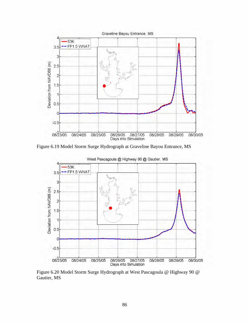
86
Figure 6.19 Model Storm Surge Hydrograph at Graveline Bayou Entrance, MS
Figure 6.20 Model Storm Surge Hydrograph at West Pascagoula @ Highway 90 @ Gautier, MS

87
Figure 6.21 Model Storm Surge Hydrograph at Escatawpa, Pascagoula River, MS
Figure 6.22 Model Storm Surge Hydrograph at Martin Bluff, West Pascagoula River, MS

88
Figure 6.23 Model Storm Surge Hydrograph at Graham Fish Camp, Pascagoula River, MS
Figure 6.24 Model Storm Surge Hydrograph at Poticaw Lodge, West Pascagoula River, MS
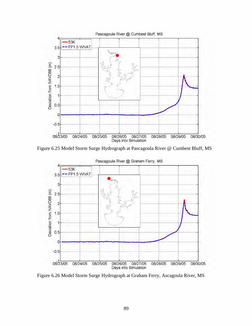
89
Figure 6.25 Model Storm Surge Hydrograph at Pascagoula River @ Cumbest Bluff, MS
Figure 6.26 Model Storm Surge Hydrograph at Graham Ferry, Ascagoula River, MS

90
Figure 6.27 Model Storm Surge Hydrograph at Moss Point, Escatawpa River, MS
Figure 6.28 Model Storm Surge Hydrograph at Pascagoula River @ Mile 1 @ Pascagoula, MS

91
Figure 6.29 Maximum Envelop of Water (Top left) FP1.5_INLET model forced by storm surge hydrograph obtained from 53K mesh domain; (Top right) FP1.5_INLET model forced by storm surge hydrograph obtained from 53K mesh domain; (Bottom) Difference of two models

92
6.2.3 Inlet-based Model with Storm Surge Hydrograph and Meteorological Forcings
(Experiments 7)
In order to examine local meteorological effects toward water surface elevations in the
Pascagoula River, Experiment 7 applies winds and pressures over the inlet-based
floodplain model (FP1.5_INLET). Also included in Experiment 7, the open-ocean
boundary is forced by a storm surge hydrograph generated from the large-domain
modeling approach (FP1.5_WNAT mesh application) so that the model results can be
compared to those generated in the previous experiment forced by storm surge
hydrograph only (see Experiment 6).
Model output from the FP1.5_INLET mesh applications of Experiments 6 and 7 is
provided for ten stations (see Figure 6.30 to Figure 6.39). The FP1.5_INLET model
output (for when it is forced by a hydrograph [calculated by the FP1.5_WNAT mesh]
only) is represented by a blue solid line and the FP1.5_INLET model output (for when it
is forced by a hydrograph [calculated by the FP1.5_WNAT mesh] and local winds and
pressures) is represented by a green dashed line. The effect of local winds and pressures
becomes apparent in different ways. For example, at the two most upstream locations in
the Pascagoula River (see Figure 6.36 and Figure 6.37), the storm surge peak is greatly
increased for when the local winds and pressures are considered. Considering the
orientation of the estuary and the track of the storm, local winds and pressures appear to
have accumulated water significantly in the upstream portions of the Pascagoula River.
Also apparent at the upstream locations (e.g., see Figure 6.38 and Figure 6.39) is the
setup and setdown of the water prior to the storm surge peak. The pressure effect causes a
93
minimal setup prior to the storm surge peak; the setdown effect is more prominent and
can be explained by the wind direction (blowing water to the south) as the storm just
begins to enter the model domain. The significant gradient in the rising limb of the storm
surge hydrograph can be explained in the reversal of wind direction to blow water (over a
sustained duration) to the north. Maximum envelopes of water (i.e. maximum height of
the storm surge) are calculated for the FP1.5_INLET mesh applications (without and with
local winds and pressures) (Figure 6.40). For when local winds and pressures are
considered, significant amounts of water are allowed to accumulate in the upstream
portions of the Pascagoula River. A difference between the two maximum envelopes of
water is calculated to highlight regions where the solutions differ. In fact, in the upstream
portions of the Pascagoula River, the local wind and pressure forcing attributes to nearly
a 2-m rise in water levels.

94
Figure 6.30 Model Storm Surge Hydrograph at Graveline Bayou Entrance, MS
Figure 6.31 Model Storm Surge Hydrograph at West Pascagoula @ Highway 90 @ Gautier, MS

95
Figure 6.32 Model Storm Surge Hydrograph at Escatawpa, Pascagoula River, MS
Figure 6.33 Model Storm Surge Hydrograph at Martin Bluff, West Pascagoula River, MS

96
Figure 6.34 Model Storm Surge Hydrograph at Graham Fish Camp, Pascagoula River, MS
Figure 6.35 Model Storm Surge Hydrograph at Poticaw Lodge, West Pascagoula River, MS

97
Figure 6.36 Model Storm Surge Hydrograph at Pascagoula River @ Cumbest Bluff, MS
Figure 6.37 Model Storm Surge Hydrograph at Pascagoula River @ Graham Ferry, MS

98
Figure 6.38 Model Storm Surge Hydrograph at Moss Point, Escatawpa River, MS
Figure 6.39 Model Storm Surge Hydrograph at Escatawpa River @ 1-10 near Orange Grove, MS

99
Figure 6.40 Maximum Envelop of Water (Top left) FP1.5_INLET model forced by storm surge hydrograph obtained from FP1.5_WNAT mesh domain; (Top right) FP1.5_INLET model forced by storm surge hydrograph obtained from FP1.5_WNAT mesh domain plus wind and pressure; (Bottom) Difference of two models

100
6.2.4 Comparison of WNAT-based Model (Experiment 4) and Inlet-based Model
(Experiment 7)
In order to verify application of the inlet-based model with a combined forcing of a storm
surge hydrograph and meteorological inputs, the inlet-based model output is compared to
the that produced by the WNAT-based model, which is considered to be the most
comprehensive mesh description. Model output from the FP1.5_INLET mesh application
(Experiment 7) is compared to model output from the FP1.5_WNAT mesh application
(Experiment 4) for ten stations (see Figure 6.41 to Figure 6.50). The FP1.5_WNAT
model output (for when it is forced by winds and pressures) is represented by a red solid
line and the FP1.5_INLET model output (for when it is forced by a hydrograph
[calculated by the FP1.5_WNAT mesh] and local winds and pressures) is represented by
a green dashed line. The similarity in the model results is expected and justifies
application of the localized domain through use of the open-ocean hydrograph (generated
by the large-scale model domain).
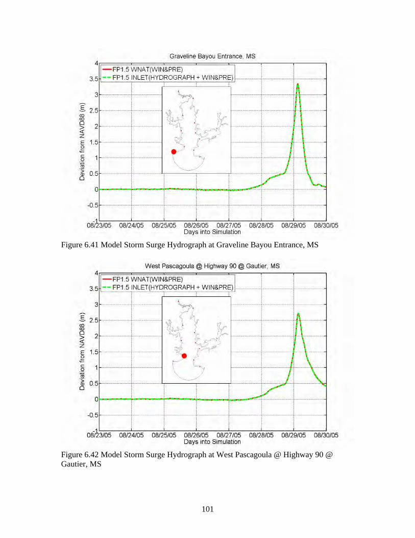
101
Figure 6.41 Model Storm Surge Hydrograph at Graveline Bayou Entrance, MS
Figure 6.42 Model Storm Surge Hydrograph at West Pascagoula @ Highway 90 @ Gautier, MS

102
Figure 6.43 Model Storm Surge Hydrograph at Escatawpa, Pascagoula River, MS
Figure 6.44 Model Storm Surge Hydrograph at Martin Bluff, West Pascagoula River, MS
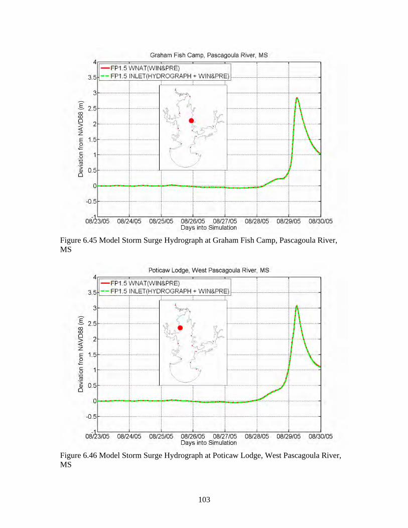
103
Figure 6.45 Model Storm Surge Hydrograph at Graham Fish Camp, Pascagoula River, MS
Figure 6.46 Model Storm Surge Hydrograph at Poticaw Lodge, West Pascagoula River, MS

104
Figure 6.47 Model Storm Surge Hydrograph at Pascagoula River @ Cumbest Bluff, MS
Figure 6.48 Model Storm Surge Hydrograph at Pascagoula River @ Graham Ferry, MS

105
Figure 6.49 Model Storm Surge Hydrograph at Moss Point, Escatawpa River, MS
Figure 6.50 Model Storm Surge Hydrograph at Escatawpa River @ 1-10 near Orange Grove, MS

106
6.2.5 Historical Data Verification
Lastly, we compare the model output to historical data (Figure 6.51 to Figure 6.55).
Recall that our interest is towards understanding the forcing mechanisms for storm surge
elevations in the Pascagoula River; it is not being claimed that the numerical model
presented herein should be used for a hindcast of Hurricane Katrina storm surge levels. In
fact, we regard it as necessary to examine the boundary forcings and model
implementations prior to any calibration to historical data. Otherwise, important physics
of the system would be folded in the model calibration process and would go undetected.
Historical stage data are provided by the LMRFC for four gauge stations located within
the Pascagoula region. The historical data are represented by the black solid line and the
FP1.5_INLET model output (for when it is forced by a hydrograph produced by the
FP1.5_WNAT mesh and local winds and pressures) is represented by the green dashed
line. It is noted that the historical data relates to the full response of the water level due to
astronomic tides, freshwater river inflow, wind-driven waves, etc., while the model
output corresponds to storm surge only.
Overall, the model captures the time of peak and the peak water level adequately. At the
first station (Figure 6.51), Pascagoula, MS, the model result is dry except for during the
storm surge peak. At the upstream stations (Cumbest Bluff and Escatawpa River), the
historical data show that water remained in the system for some time after the peak storm
surge (Figure 6.53 and Figure 6.55). Clearly, freshwater river inflows played a role in the
recession of the storm surge; while the timing and level of the storm surge peak was well-
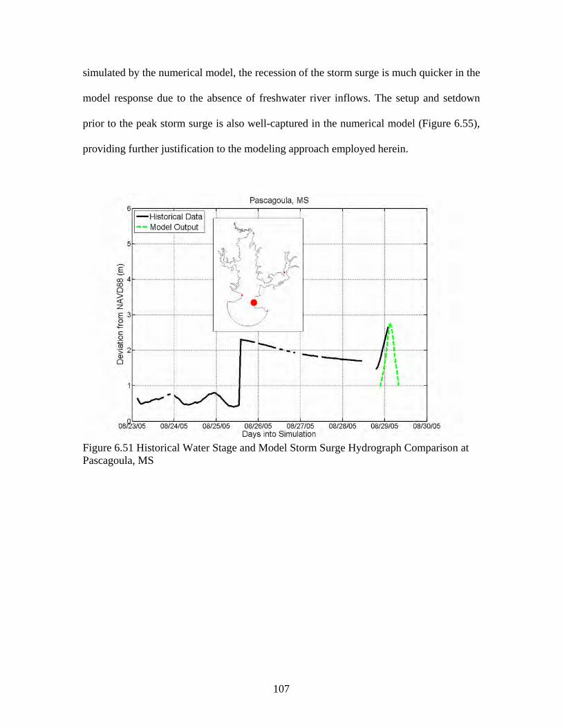
107
simulated by the numerical model, the recession of the storm surge is much quicker in the
model response due to the absence of freshwater river inflows. The setup and setdown
prior to the peak storm surge is also well-captured in the numerical model (Figure 6.55),
providing further justification to the modeling approach employed herein.
Figure 6.51 Historical Water Stage and Model Storm Surge Hydrograph Comparison at Pascagoula, MS
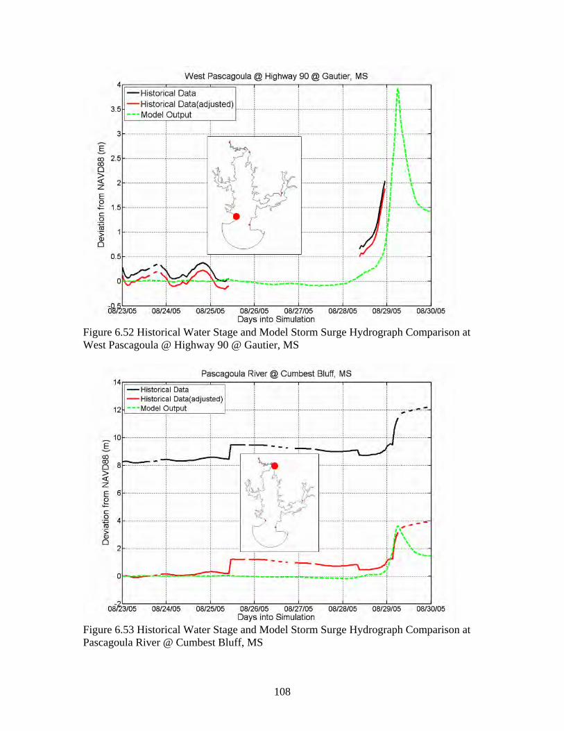
108
Figure 6.52 Historical Water Stage and Model Storm Surge Hydrograph Comparison at West Pascagoula @ Highway 90 @ Gautier, MS
Figure 6.53 Historical Water Stage and Model Storm Surge Hydrograph Comparison at Pascagoula River @ Cumbest Bluff, MS

109
Figure 6.54 Historical Water Stage and Model Storm Surge Hydrograph Comparison at Graham Ferry, Pascagoula River, MS
Figure 6.55 Historical Water Stage and Model Storm Surge Hydrograph Comparison at Escatawpa River @ 1-10 near Orange Grove, MS
110
CHAPTER 7. CONCLUSIONS AND FUTURE WORK
Chapter 7 presents the conclusions that resulted from conducting this research along with
future efforts associated with the work. One objective of this study was to develop a
floodplain DEM for the Pascagoula River in order to develop a numerical model that will
allow for an understanding of the storm surge dynamics within the Pascagoula River.
First, we developed a 1.5-m contour floodplain model domain which covers the marsh
areas concerning the Lower Pascagoula and Escatawpa Rivers. Then the inlet-based
floodplain model was incorporated into the large-scale (WNAT-53K) computational
mesh. In this study, applications of the 53K, WNAT- and inlet-based floodplain meshes
are performed under different forcing implementations, involving astronomic tides, storm
surge hydrographs and meteorological forcing (winds and pressures) in isolation (i.e., as
the single forcing mechanism) and collectively (i.e., together in combination).
7.1 Conclusions
First, a 1.5-m floodplain mesh was constructed to allow for the overtopping of the river
banks. This floodplain model was applied in an astronomic tide simulation to show
improvement upon earlier model results which involved an in-bank-only hydrodynamic
description. It is learned from these model intercomparisons that the floodplains become
important towards modeling astronomic tides within the Pascagoula River. It is further
concluded that a 1.5-m boundary is sufficient to capture any tidally driven storage
because of the minimal tidal amplitudes within the Pascagoula River (less than 1 m).
111
Next, the inlet-based floodplain mesh is incorporated into the WNAT-53K model domain
to produce a large-scale computational mesh that focuses on the local region of interest.
The resulting large-scale modeling domain employs a refined coastline and has the
barrier islands located along the Gulf Coast meshed over in order to allow for the wetting
and drying of elements. Winds and pressures associated with Hurricane Katrina (August
23 to 30, 2005) are applied over the large-scale computational mesh which includes the
high resolution of the Pascagoula River (FP1.5_WNAT). Model output is specified at
points located along a 2.5-km-radius semi-circular arc (centered on the Pascagoula River
inlet entrances) in order to examine storm surge hydrographs that will be used to drive a
localized domain of the Pascagoula River. The WNAT-53K mesh is applied in a similar
simulation (winds and pressures) to provide model output at the same arc points. The two
model solutions (FP1.5_WNAT; WNAT-53K) are compared to one another to determine
that the barrier islands can impact flow. For the WNAT-53K mesh, the barrier islands are
defined with no-flow boundary constraints which allows the water to accumulate to
greater heights (relative to those produced by the FP1.5_WNAT mesh) behind the barrier
islands and up to the coastline. On other hand, the FP1.5_WNAT mesh allows for the
wetting and drying of those elements, which permits for the storm surge to overtop the
barrier islands and approach the coastline directly.
It is then demonstrated that a hydrograph generated by the FP1.5_WNAT mesh can be
applied on the open-ocean boundary of the localized floodplain mesh (FP1.5_INLET) in
order to produce results in the interior that are identical to those produced by the

112
FP1.5_WNAT mesh. Finally, the localized domain is tested by imposing the hydrograph
boundary condition together with local winds and pressures.
When interested in storm surge levels along the Gulf Coast of the United States, a
numerical model must describe the barrier islands with elements that are allowed to wet
and dry (as opposed to using a no-flow boundary constraint). For when a localized
domain is demanded, it is necessary to account not only for the local wind and pressure
forcing, but also for the remote effects of the wind and pressure forcing. These remote
effects of the meteorological forcings can only be captured by a large-scale model
domain. The remote meteorological effect can be incorporated into a localized domain
through a storm surge hydrograph that is calculated by a large-scale computational
domain. The local winds and pressures together with the hydrograph boundary forcing
(generated by a large domain) then become sufficient to drive the localized mesh.
7.2 Future Work
The tasks completed in this thesis have provided valuable guidance that will allow one to
expand on the overall work regarding the calculation of storm tide elevations in the
Pascagoula River. First, the maximum envelopes of water presented in Figure 6.18,
Figure 6.29, and Figure 6.40 all indicate maximum water levels at the floodplain
boundary of at least 1.75 m. With a 1.5-m floodplain boundary, water levels in excess of
1.5 m are not allowed to spill out further into the floodplain as would occur in reality.
While the 1.5-m floodplain mesh is shown to be a vast improvement upon the in-bank
mesh by allowing for the overtopping of the river banks, future work associated with this
113
project will need to focus on extending the inundation areas to the 5-m contour (Figure
7.1) to permit for the additional storage.
Second, freshwater river inflows are identified as the next hydrodynamic forcing to be
introduced to the numerical model. The contribution of freshwater river inflows would
increase the volume of accumulated storm surge within the Pascagoula River and
adjacent floodplains, and also might affect the recession of the storm surge as the
increased volume exits the system through the two inlets. Once knowledge is gained with
respect to the inclusion of freshwater river inflows in the numerical model, then all long-
wave components (i.e., astronomic tides; freshwater river inflows, local and remote
meteorological effects) of the storm tide can be modeled together in a single simulation.
Ultimately, a recreation of the water levels caused by Hurricane Katrina would require a
description of the wind-driven waves and their effect on the overall storm tide. Only until
short-wave effects are combined (and interacting) with the long-wave components of the
storm tide can one begin a true hindcast of the Hurricane Katrina water levels.

114
Figure 7.1 SL15: Up to 5.0 m above MSL Contours

115
APPENDIX A. SAFFIR SIMPSON HURRICANE SCALE

116
The Saffir-Simpson Hurricane Scale is a 1-5 rating based on the hurricane's present
intensity. This is used to give an estimate of the potential property damage and flooding
expected along the coast from a hurricane landfall. Wind speed is the determining factor
in the scale, as storm surge values are highly dependent on the slope of the continental
shelf and the shape of the coastline, in the landfall region. Note that all winds are using
the U.S. 1-minute average.
Figure A.1 Saffir-Simpson Scale

117
APPENDIX B. STORM SURGE HEIGHT DATA SET
RECORDED BY THE SURVEY TEAM IN THE IMMEDIATE AFTERNOON OF
HURRICANE KATRINA
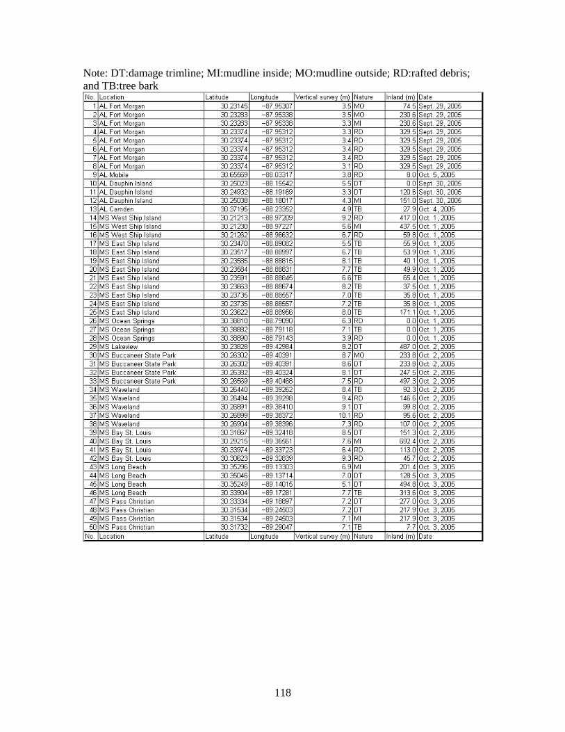
118
Note: DT:damage trimline; MI:mudline inside; MO:mudline outside; RD:rafted debris; and TB:tree bark

119

120

121
APPENDIX C. TIDAL CONSTITUENTS EMPLOYED BY ADCIRC-2DDI

122
Table C.1 23 Tidal constituents applied in ADCIRC harmonic analysis
Constituent Description Frequency (rad/s) Degrees per solar hour
STEADY Principal water level 0.000000000000000 0.0000 MN4 Lunar monthly constituent 0.000000420111582 0.5445
SM Lunisolar synodic fortnightly constituent 0.000000783620452 1.0156
O1 Lunar diurnal constituent 0.000010756574418 13.9405 K1 Lunar diurnal constituent 0.000011608900776 15.0451
MNS2 Arising from interaction between MN and S2 0.000021159184779 27.4223
2MS2 Variational constituent 0.000021593421780 27.9851
N2 Larger lunar elliptic semi-diurnal constituent 0.000021962189894 28.4630
M2 Principal lunar semi-diurnal constituent 0.000022343772344 28.9575
2MN2 Smaller lunar elliptic semi-diurnal constituent 0.000022783610382 29.5276
S2 Principal solar semi-diurnal constituent 0.000023148148148 30.0000
2SM2 Shallow-water semi-diurnal constituent 0.000023913376186 30.9917
MN4 Shallow-water quarter diurnal constituent 0.000044345111395 57.4713
M4 Shawllow-water overtides of principal lunar constituent 0.000044687544688 57.9151
MS4 Shallow-water quarter diurnal constituent 0.000045567220764 59.0551
2MN6 Shallow-water twelfth diurnal constituent 0.000066517667092 86.2069
M6 Shawllow-water overtides of principal lunar constituent 0.000066902162278 86.7052
MSN6 Arising from interaction between M2, N2 and S2 0.000067291128338 87.2093
M8 Shallow-water eighth diurnal constituent 0.000089721504450 116.2791
M10 Shallow-water tenth diurnal constituent 0.000111289173789 144.2308
P1 Solar diurnal constituent 0.000011539455707 14.9551 K2 Lunisolar semi-diurnal constituent 0.000025777447826 33.4076
Q1 Larger lunar elliptic diurnal constituent 0.000010333994709 13.3929

123
Table C.2 37 Tidal constituents used in the resynthesis of the historical tidal records for the NOS stations.
Constituent Tidal species Frequency (rad/s) Degrees per solar hour
SA long-period 0.000000199106190 0.2580 SSA long-period 0.000000398212870 0.5161 MM long-period 0.000002639203000 3.4204 MSF long-period 0.000004925201800 6.3831 MF long-period 0.000005323414700 6.8991 2Q1 diurnal 0.000062319338000 80.7659 Q1 diurnal 0.000064958541000 84.1863 RHO1 diurnal 0.000065311745000 84.6440 O1 diurnal 0.000067597744000 87.6067 M1 diurnal 0.000070281955000 91.0854 P1 diurnal 0.000072522946000 93.9897 S1 diurnal 0.000072722052000 94.2478 K1 diurnal 0.000072921158000 94.5058 J1 diurnal 0.000075560361000 97.9262 OO1 diurnal 0.000078244573000 101.4050 2N2 semi-diurnal 0.000135240500000 175.2717 MU2 semi-diurnal 0.000135593700000 175.7294 N2 semi-diurnal 0.000137879700000 178.6921 NU2 semi-diurnal 0.000138232900000 179.1498 M2 semi-diurnal 0.000140518900000 182.1125 LDA2 semi-diurnal 0.000142804900000 185.0752 L2 semi-diurnal 0.000143158110000 185.5329 T2 semi-diurnal 0.000145245010000 188.2375 S2 semi-diurnal 0.000145444100000 188.4956 R2 semi-diurnal 0.000145643200000 188.7536 K2 semi-diurnal 0.000145842320000 189.0116 2SM2 semi-diurnal 0.000150369310000 194.8786 2MK3 terdiurnal 0.000208116650000 269.7192 M3 terdiurnal 0.000210778350000 273.1687 MK3 terdiurnal 0.000213440060000 276.6183 MN4 fourth-diurnal 0.000278398600000 360.8046 M4 fourth-diurnal 0.000281037810000 364.2250 MS4 fourth-diurnal 0.000285963010000 370.6081 S4 fourth-diurnal 0.000290888210000 376.9911 M6 sixth-diurnal 0.000421556710000 546.3375

124
Constituent Tidal species Frequency (rad/s) Degrees per solar hour
S6 sixth-diurnal 0.000436332310000 565.4867 M8 eighth-diurnal 0.000562075610000 728.4500

125
Table C.3 35 Tidal constituents at the USGS stations extracted by T_TIDE
Constituent Tidal species Frequency (rad/s) Degrees per solar hour
MM long-period 0.000002639286895 3.4205 MSF long-period 0.000004925144616 6.3830 ALP1 diurnal 0.000060033392149 77.8033 2Q1 diurnal 0.000062319424403 80.7660 Q1 diurnal 0.000064958536765 84.1863 O1 diurnal 0.000067597823660 87.6068 NO1 diurnal 0.000070281965517 91.0854 K1 diurnal 0.000072921077879 94.5057 J1 diurnal 0.000075560364774 97.9262 OO1 diurnal 0.000078244506630 101.4049 UPS1 diurnal 0.000080883793525 104.8254 EPS2 semi-diurnal 0.000132954470028 172.3090 MU2 semi-diurnal 0.000135593756923 175.7295 N2 semi-diurnal 0.000137879614644 178.6920 M2 semi-diurnal 0.000140518901539 182.1125 L2 semi-diurnal 0.000143158188434 185.5330 S2 semi-diurnal 0.000145444046155 188.4955 ETA2 semi-diurnal 0.000148481442652 192.4319 MO3 terdiurnal 0.000208116725199 269.7193 M3 terdiurnal 0.000210778352309 273.1687 MK3 terdiurnal 0.000213439979418 276.6182 SK3 terdiurnal 0.000218365298567 283.0014 MN4 fourth-diurnal 0.000278398516183 360.8045 M4 fourth-diurnal 0.000281037803078 364.2250 SN4 fourth-diurnal 0.000283323835332 367.1877 MS4 fourth-diurnal 0.000285962947694 370.6080 S4 fourth-diurnal 0.000290888266843 376.9912 2MK5 fifth-diurnal 0.000353958880957 458.7307 2SK5 fifth-diurnal 0.000363809344722 471.4969 2MN6 sixth-diurnal 0.000418917592255 542.9172 M6 sixth-diurnal 0.000421556704617 546.3375 2MS6 sixth-diurnal 0.000426481849233 552.7205 2SM6 sixth-diurnal 0.000431407168382 559.1037 3MK7 seventh-diurnal 0.000494477782496 640.8432 M8 eighth-diurnal 0.000562075606156 728.4500

126
APPENDIX D. ADCIRC-2DDI INPUT FILE: SINGLE METROLOGICAL
INPUT FILE (FORT.22) USED FOR WNAT-53K MESH DOMAIN
(TOTAL COMPUTATINAL NODES: 52774)
Table 7.1 Legend for Fort.22
Parameter
name
JN WSX, WSY PRN
Definition Node number Applied horizontal wind stress
in the x, y directions divided
by the reference density of
water
Applied
atmospheric
pressure at the free
surface.
Unit Dimensionless m/s m/s mb
pmin= 985. v = 32.22(m/s)
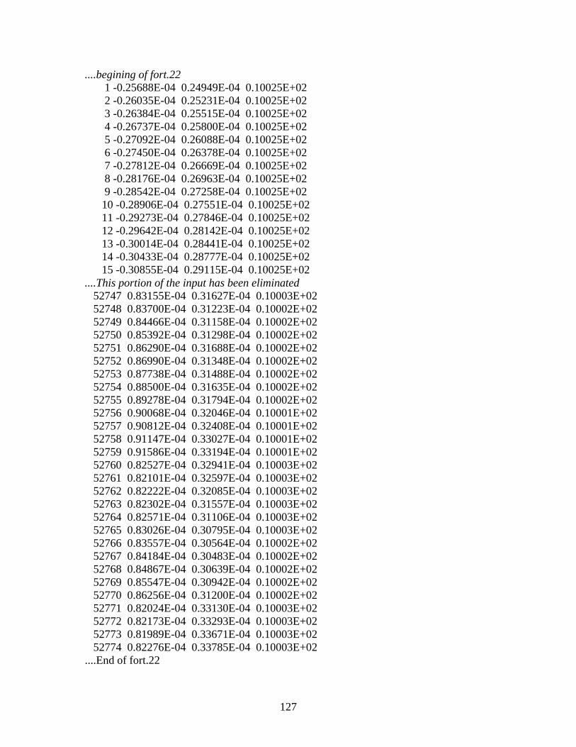
127
....begining of fort.22 1 -0.25688E-04 0.24949E-04 0.10025E+02 2 -0.26035E-04 0.25231E-04 0.10025E+02 3 -0.26384E-04 0.25515E-04 0.10025E+02 4 -0.26737E-04 0.25800E-04 0.10025E+02 5 -0.27092E-04 0.26088E-04 0.10025E+02 6 -0.27450E-04 0.26378E-04 0.10025E+02 7 -0.27812E-04 0.26669E-04 0.10025E+02 8 -0.28176E-04 0.26963E-04 0.10025E+02 9 -0.28542E-04 0.27258E-04 0.10025E+02 10 -0.28906E-04 0.27551E-04 0.10025E+02 11 -0.29273E-04 0.27846E-04 0.10025E+02 12 -0.29642E-04 0.28142E-04 0.10025E+02 13 -0.30014E-04 0.28441E-04 0.10025E+02 14 -0.30433E-04 0.28777E-04 0.10025E+02 15 -0.30855E-04 0.29115E-04 0.10025E+02 ....This portion of the input has been eliminated 52747 0.83155E-04 0.31627E-04 0.10003E+02 52748 0.83700E-04 0.31223E-04 0.10002E+02 52749 0.84466E-04 0.31158E-04 0.10002E+02 52750 0.85392E-04 0.31298E-04 0.10002E+02 52751 0.86290E-04 0.31688E-04 0.10002E+02 52752 0.86990E-04 0.31348E-04 0.10002E+02 52753 0.87738E-04 0.31488E-04 0.10002E+02 52754 0.88500E-04 0.31635E-04 0.10002E+02 52755 0.89278E-04 0.31794E-04 0.10002E+02 52756 0.90068E-04 0.32046E-04 0.10001E+02 52757 0.90812E-04 0.32408E-04 0.10001E+02 52758 0.91147E-04 0.33027E-04 0.10001E+02 52759 0.91586E-04 0.33194E-04 0.10001E+02 52760 0.82527E-04 0.32941E-04 0.10003E+02 52761 0.82101E-04 0.32597E-04 0.10003E+02 52762 0.82222E-04 0.32085E-04 0.10003E+02 52763 0.82302E-04 0.31557E-04 0.10003E+02 52764 0.82571E-04 0.31106E-04 0.10003E+02 52765 0.83026E-04 0.30795E-04 0.10003E+02 52766 0.83557E-04 0.30564E-04 0.10002E+02 52767 0.84184E-04 0.30483E-04 0.10002E+02 52768 0.84867E-04 0.30639E-04 0.10002E+02 52769 0.85547E-04 0.30942E-04 0.10002E+02 52770 0.86256E-04 0.31200E-04 0.10002E+02 52771 0.82024E-04 0.33130E-04 0.10003E+02 52772 0.82173E-04 0.33293E-04 0.10003E+02 52773 0.81989E-04 0.33671E-04 0.10003E+02 52774 0.82276E-04 0.33785E-04 0.10003E+02 ....End of fort.22

128
LIST OF REFERENCES
Bacopoulos, P. (2006). “Analysis, modeling, and simulation of the tides in the Loxahatchee River estuary (Southeastern Florida).” University of Central Florida, Orlando, FL. Master's Thesis.
Bacopoulos, P., Y. Funakoshi, S. C. Hagen, A. T Cox, and V. J. Cardone (2008).
“The role of meteorological forcing on the St. Johns River (Northeastern Florida).” Journal of Hydrology (in press).
Blain, C. A., J. J. Westerink, and R. A. Jr. Luettich, (1994).
“The influence of domain size on the response characteristics of a hurricane storm surge model.” Journal of Geophysical Research 99(C9): 18467-18479.
Blain, C. A., J. J. Westerink, and R. A. Jr. Luettich, (1998).
“Grid convergence studies for the prediction of hurricane storm surge.” International Journal for Numerical Methods in Fluids 26: 369-401.
Bode, L. and T. A. Hardy (1997). “Progress and recent developments in storm surge modeling.” Journal of
Hydraulic Engineering 123(4): 315-331. Ceyhan, E., P. Basuchowdhuri, T. Judeh, S. Ou, B. Estrade, and T. Kosar (2007).
“Towards a faster and improved ADCIRC (ADvanced Multi-Dimensional CIRCulation) model.” Journal of Coastal Research, Special Issue 50
Chen, Q., L. Wang, H. Zhao, and S. L. Douglass (2007).
“Prediction of Storm Surges and Wind Waves on Coastal Highways in Hurricane-Prone Areas.” Journal of Coastal Research 23(5): 1304-1317
Department of the Army; U.S. Army Corps of Engineers (2007).
“Intent to prepare a draft supplemental environmental impact statement to evaluate construction of authorized improvements to the federal Pascagoula Harbor navigation project in Jackson County, MS.”
Dietsche, D., S. C. Hagen, and P. Bacopoulos (2007).
“Storm surge simulations for Hurricane Hugo (1989): On the significance of inundation areas.” Journal of Waterway, Port, Coastal, and Ocean Engineering 133(3): 183-191.
Droppo, Ian G. (2003).
“Preserving the Pascagoula: D.G. Schueler.” University Press of Mississippi.

129
Fritza, H. M., C. Blounta, R. Sokoloskia, J. Singletona, A. Fuggleb, B.G. McAdooc, A. Moored, C. Grassa and B. Tate (2007).
“Hurricane Katrina storm surge distribution and field observations on the Mississippi Barrier Islands Estuarine.” Coastal and Shelf Science 74(1-2): 12-20
Funakoshi, Y. (2006).
“Coupling of hydrodynamic and wave models for storm tide simulations: A case study for Hurricane Floyd (1999).” University of Central Florida. Orlando, FL. Ph.D. Dissertation.
Graber, H. C., V. J. Cardone, R. E. Jensen, D. N. Slinn, S. C. Hagen, A. T. Cox, M. D. Powell, and C. Grassl (2006).
“Coastal forecasts and storm surge predictions for tropical cyclones: A timely partnership program.” Oceanography 19(1): 130-141.
Hagen, S. C. and D. M Parrish (2004).
“Meshing requirements for tidal modeling in the western North Atlantic.” International Journal of Computational Fluid Dynamics 18(7): 585-595.
Hagen, S. C., J. J. Westerink, et al. (2000).
“One-dimensional finite element grids based on a localized truncation error analysis.” International Journal for Numerical Methods in Fluids 32: 241-261.
Hagen, S. C., J. J. Westerink, et al. (2001).
“Two-dimensional, unstructured mesh generation for tidal models.” International Journal for Numerical Methods in Fluids 35: 669-686.
Hagen, S.C., A.K. Zundel, et al. (2006).
“Automatic, Unstructured Mesh Generation for Tidal Calculations in a Large Domain.” International Journal of Computational Fluid Dynamics 20(8): 593-608.
IPET Force - U.S. Army Corps. of Engineers (2007).
“Performance evaluation of the New Orleans and Southeast Louisiana Hurricane Protection System.” Vicksburg, MS.
Kohut, J. T., S. M. Glenn, and J. D. Paduan, (2006).
“Inner shelf response to Tropical Storm Floyd.” Journal of Geophysical Research 111(C09S91): 1-18.
Kolar, R. L., W. G. Gray, et al. (1994).
“Shallow water modeling in spherical coordinates: Equation formulation, numerical implementation, and application.” Journal of Hydraulic Research 32(1): 3-24.
Kolar, R. L., J. J. Westerink, et al. (1994).

130
“Aspects of non-linear simulations using shallow water models based on the wave continuity equation.” Computers and Fluids 23(3): 523-538.
Luettich, R. A. Jr. and J. J Westerink (2000).
“ADCIRC: A (parallel) advanced circulation model for oceanic, coastal and estuarine waters.” Users manual, http://www.marine.unc.edu/C_CATS/adcirc/adcirc.htm.
Luettich, R.A., S.D. Carr, et al. (2002).
“Semi-diurnal seiching in a shallow, micro-tidal lagoonal estuary.” Continental Shelf Research 22: 1669-1681.
Massey, W. G., J. W. Gangai, E. Drei-Horgan, and K. J. Slover (2007).
“History of Coastal Inundation Models.” Marine Technology Society Journal 41(1): 7-17
Mossa, J. and D. Coley (2004).
“Planform charge rates in rivers with and without instream and floodplain sand and gravel mining: Assessing instability in the Pascagoula River and Tributaries, Mississippi.” Gainesville, FL, University of Florida.
Murray, R. R. (2003).
“A sensitivity analysis for a tidally-influenced riverine system.” University of Central Florida. Orlando, FL. Master's Thesis.
Oldham, M. B. Jr. and J. W. Rushing (1970).
“Water resuorces planning for Pascagoula Basin.” Journal of the Waterways and Harbors Division, Proceedings of the America Society of Civil Engineers 96(WW1): 65-85.
Parrish, D. M. (2001).
“Development of a tidal constituent database for the St. Johns River Water Management District.” University of Central Florida. Orlando, FL. Master's Thesis.
Parrish, D.M. and S. C. Hagen (2007).
“2D, unstructured mesh generation for oceanic and coastal tidal models from a localized truncation error analysis with complex derivatives.” International Journal of Computational Fluid Dynamics 21(7&8): 277-296.
Pascagoula Harbor (1997).
“Pascagoula Harbour, Mississippi - condition of improvement on 30 September 1997.”
Pawlowicz, R., B. Beardsley, et al. (2002).
131
“Classical tidal harmonic analysis including error estimates in MATLAB using T_TIDE.” Computers and Geosciences 28: 929-937.
Peng, M., L. Xie, and L. J. Pietrafesa, (2006). “A numerical study on hurricane-induced storm surge and inundation in Charleston Harbor, South Carolina.” Journal of Geophysical Research 111(C8): 1-22.
Reid, R. O. (1990).
“Waterlevel changes, tides and storm surges.” Handbook of Ciastal and Ocean Engineering. Pulisher. Houston, Texas, J. Herbich.
Reid, R. O. and B. R. Bodine (1968). “Numerical Model for Storm Surges in Galveston Bay,” American Society of Civil Engineers: Journal of the Harbors and harbors Division 94(WW1): 33-57.
Salisbury, M. B. and S. C. Hagen (2007).
“The Effect of Tidal Inlets on Open Coast Storm Surge Hydrographs.” Coastal Engineering 54: 377-391.
Shen, J., H.Wang, M. Sisson, and W. Gong (2006). “Storm tide simulation in the Chesapeake Bay using an unstructured grid model.” Estuarine, Coastal and Shelf Science 68:1-16.
Shen, J, K. Zhang, C. Xiao, and W. Gong (2006).
“Improved Prediction of Storm Surge Inundation with a High-Resolution Unstructured Grid Model.” Journal of Coastal Research 22(6): 1309-1319
Smith, J. M. (2006).
“Modeling Nearshore Waves for Hurricane Katrina” 9th Internatinal Workshop on Wave hindcasting and forecasting, Victoria, B.C., Canada.
The Port of Pascagoula. (2008).
“The history of the Port of Pascagoula.” Retrieved May 13th, 2008 from http://www.portofpascagoula.com/.
Turnipseed, D. P. and J. B. Storm (1995).
“Streamflow characteristics of the Lower Pascagoula River, Mississippi.” Proceedings of the Twenth-fifth Mississippi Water Resources Conference, Jaskson, MS.
U.S. Army Corps of Engineers (1968).
“Pascagoula River comprehensive basin study.” Mobile, Alabama. Valle-Levinson, A., K. C.Wong, and K. T. Bosley (2002).

132
“Response of the lower Chesapeake Bay to forcing from Hurricane Floyd.” Continental Shelf Research 22: 1715-1729.
Veeramony, J. and C.A. Blain (2001).
“Barotropic flow in the vicinity of an idealized inlet – Simulations with the ADCIRC model.” Washington, D.C., Naval Research Laboratory.
Walters, R. A. and R. T. Cheng (1979).
“A two-dimensional hydrodynamic model of a tidal estuary.” Advances in Water Resources 2: 177-184.
Wang, Qing (2008). “Finite element modeling of tides and currents of the Pascagoula River.” MS thesis, University of Central Florida, Orlando, Florida.
Warner, J. C., W. R. Geyer, et al. (2005). “Numerical modeling of an estuary: A comprehensive skill assessment.” Journal of Geophysical Research-Oceans 110(C5): 1-13.
Westerink, J. J., C. A. Blain, et al. (1994).
“ADCIRC: An advanced three-dimensional circulation model for shelves, coasts, and estuaries, II: User's manual for ADCIRC-2DDI. Technical Report DRP-92-6.” U.S. Army Corps of Engineers, Waterways Experiment Station, Vicksburg, Mississippi.
Westerink, J. J., R. A. Jr. Luettich, et al. (1994).
“Modeling tides in the western North Atlantic using unstructured graded grids.” Tellus 46A: 178-199.
Westerink, J. J., R. A. Tr. Luettich, A. M. Baptista, N. W. Scheffner, and P. Farrar (1992).
“Tide and storm surge predictions using finite element model.” Journal of Hydraulic Engineering 118: 1373-1390.
Westerink et al. (2004).
“A New Generation Hurricane Storm Surge Model for Southern Louisiana” ADCIRC Development Group Publications.
Wright, J. (2000).
“Waves, tides and shallow-water processes.” Butterworth-Heinemann/Open University, Oxford, UK.