THE PENNSYLVANIA STATE UNIVERSITY

SCHREYER HONORS COLLEGE

DEPARTMENT OF MECHANICAL AND NUCLEAR ENGINEERING

SIMULATION OF A VEHICLE DOCKING AND COLLISION AVOIDANCE SYSTEM USING LIDAR-BASED OBJECT TRACKING

KYLE REIGH SUMMER 2013

A thesis submitted in partial fulfillment

of the requirements for a baccalaureate degree in Mechanical Engineering

with honors in Mechanical Engineering

Reviewed and approved* by the following:

Sean Brennan Associate Professor of Mechanical Engineering

Thesis Supervisor

H. Joseph Sommer III Professor of Mechanical Engineering

Honors Adviser

* Signatures are on file in the Schreyer Honors College.

i

ABSTRACT

With advances in range finding technology and computing power, vehicle automation is

becoming increasingly commonplace. One of the requirements for these vehicles is to meet or

exceed the performance of human operators in reacting to changes in the environment. These

automation systems must follow lane lines, locate and track nearby objects, and avoid these

objects if possible. This is true for a variety of tasks and operations from highway driving to

parking.

This thesis designs a system to automate a vehicle docking system for possible use in

commercial applications. In this system, all of the hardware, excluding what is necessary for

vehicle steering, is located on the dock. This allows for a variety of vehicles to be used, as the

range finding and the majority of processing equipment remains on the dock rather than on the

individual vehicles. To test the feasibility of this system, a simulation is developed that

represents the key subsystems that are necessary: lane following, object tracking, and collision

avoidance. A steering control system is presented to guide the vehicle through a straight lane that

leads to the dock. A simulated LIDAR scans the operating area, and a tracking algorithm is

implemented to identify objects that may interrupt the vehicles progress. Finally, a decision

making process is introduced that attempts to avoid objects when a collision is imminent. The

result is a simulation that guides the vehicle to its final destination while avoiding any objects that

may enter its path.

ii

TABLE OF CONTENTS

List of Figures .......................................................................................................................... iii

List of Tables ........................................................................................................................... iv

Acknowledgements .................................................................................................................. v

Chapter 1 Introduction ............................................................................................................. 1

1.1 Motivation .............................................................................................................. 1 1.2 Lane Following ...................................................................................................... 2 1.3 Object Tracking ...................................................................................................... 2 1.4 Collision Avoidance ............................................................................................... 3 1.5 Thesis Organization ............................................................................................... 3

Chapter 2 Related Work........................................................................................................... 5

2.1 Lane Following ...................................................................................................... 5 2.1.1 Lane Detection ............................................................................................ 5 2.1.2 Lane Following ........................................................................................... 6

2.2 Laser-based Object Tracking ................................................................................. 7 2.2.1 Pre-processing ............................................................................................. 7 2.2.2 Segmentation and Classification ................................................................. 8 2.2.3 Data Association ......................................................................................... 11 2.2.4 Filtering ....................................................................................................... 12

2.3 Collision Avoidance ............................................................................................... 13 2.3.1 Search Space ............................................................................................... 13 2.3.2 Path Optimization ........................................................................................ 14

Chapter 3 System Setup ........................................................................................................... 15

3.1 LIDAR ................................................................................................................... 15 3.2 Vehicle ................................................................................................................... 16

Chapter 4 Lane Following and Vehicle Control ...................................................................... 19

4.1 Lane Detection ....................................................................................................... 19 4.2 Vehicle Control ...................................................................................................... 19

4.2.1 Vehicle Model ............................................................................................. 20 4.2.2 Lookahead Point .......................................................................................... 21 4.2.3 PD Control................................................................................................... 22

4.3 Performance ........................................................................................................... 23

Chapter 5 Object Detection ...................................................................................................... 25

iii

5.1 LIDAR Simulation ................................................................................................. 25 5.2 Object Tracking ...................................................................................................... 26

5.2.1 Pre-processing ............................................................................................. 26 5.2.2 Segmentation ............................................................................................... 26 5.2.3 Data Association ......................................................................................... 27

5.3 Performance ........................................................................................................... 28

Chapter 6 Collision Avoidance ................................................................................................ 30

6.1 Proximity Measurement ......................................................................................... 30 6.2 Braking ................................................................................................................... 31 6.3 Turning ................................................................................................................... 32

Chapter 7 Experimental Results ............................................................................................... 33

7.1 Results .................................................................................................................... 33 7.1.1 Stationary Object ......................................................................................... 33 7.1.2 Object with Constant Velocity .................................................................... 35 7.1.3 Object with Acceleration ............................................................................. 36 7.1.4 Multiple Objects .......................................................................................... 37

7.2 Failure Analysis ..................................................................................................... 37

Chapter 8 Conclusion ............................................................................................................... 38

BIBLIOGRAPHY ............................................................................................................ 39

iv

LIST OF FIGURES

Figure 2-1. Geometry of the polar coordinates of the Hough Transform [17].........................

Figure 2-2. Example of DBSCAN in which p and q are density connected, and B is noise [1]. ....................................................................................................................................

Figure 2-3. Example of voting scheme classification results [7]. ............................................

Figure 2-4. Example of the dynamic velocity window for collision avoidance [20]. ..............

Figure 3-1. Diagram of lane lines and vehicle starting position. LIDAR is located at the origin. ...............................................................................................................................

Figure 4-1. Control system diagram for lane following ...........................................................

Figure 4-2. Vehicle geometry for dynamics model [18]. ........................................................

Figure 4-3. Geometry of lookahead point [18]. .......................................................................

Figure 4-4. Vehicle location at 3 different times during the lane following process. Left is the starting point with the path planned. Middle is the vehicle after 3 seconds. Right is the vehicle after 6 seconds. ...........................................................................................

Figure 5-1. An example of a simulated LIDAR scan ..............................................................

Figure 5-2. Sample tracking of vehicle and two objects .......................................................... 29

Figure 7-1. Successful braking to avoid a stationary object .................................................... 34

Figure 7-2. Y-position vs. time of a successful braking maneuver to avoid a stationary object ................................................................................................................................ 34

Figure 7-3. Successful braking to avoid an object with constant velocity ............................... 35

Figure 7-4. Y-position vs. time of vehicle for a successful braking maneuver to avoid a constant velocity object .................................................................................................... 36

v

LIST OF TABLES

Table 3-1. List of simulated vehicle properties. ....................................................................... 17

1

Chapter 1

Introduction

1.1 Motivation

Vehicle automation is a field that is rapidly growing. With these advances, safety is

always a primary concern. As object tracking and vehicle control technology improves, more

applications become possible that meet high standards of safety.

Parking or docking is a task necessary for a variety of vehicle types that is

straightforward and does not usually require the very complex decision from a human operator.

This makes it an ideal candidate for automation. An example of this is parking assistance that can

be found in many consumer automobiles. A new problem arises when the process is scaled up,

however, as may be the case in large fleet operations. Here, there is a much greater chance of an

object entering the path of the docking vehicle. These obstacles may include, but are not limited

to, people and other vehicles. A system is necessary to detect these obstacles from afar in order

to bring the vehicle to a stop before there is a collision.

Before such a system can be implemented or even prototyped, other tests must be

administered, including a simulation of the docking process, to check the feasibility. While a

simulation like this may not replicate all of the finer details a physical prototype might, it

provides sufficient data to continue in the design process.

2

1.2 Lane Following

First, the vehicle must be guided to the dock assuming there are no obstructions in its

path. Vehicle position and orientation are found through the object detection system as well as

lane location. Using the lane markers, a path can be planned for the vehicle to follow. The

vehicle will proceed forward along this path at a constant velocity. Proportional-Derivative

control can be added to assure that the vehicle follows this path as it moves forward. The steering

input in this situation is assumed to be a control relative to the error in a look-ahead point directly

in front of the vehicle. A low-speed bicycle model can be used to find the vehicle response from

the controlled steering input. The vehicle will proceed following the predetermined path as long

as there are no objects entering the path.

1.3 Object Tracking

For a docking system to successfully avoid collision with obstacles, it must first be able

to detect and track them. A variety of methods are available that can capture some combination

of range or feature data in order to locate moving objects: radar, camera systems, ultrasonic

sensors, etc, and each has its own advantages. Among these, laser-based tracking systems have

some distinct qualities that many other devices lack. LIDAR is a common device that allows for

the acquisition of range data based on a fixed sweep of a laser. It is an active sensor, and thus is

difficult to confuse with spurious external signals. It is possible for the LIDAR to rotate a full

360 degrees, though it is often limited to 180, allowing for a field of view much larger than that

of other devices. It also has a large functional range and high resolution, allowing for accurate

data even at a far distance.

3

Range data points are collected each sweep of the LIDAR. Points that correspond to a

known background range can then be removed, leaving only points that were not there

previously. These points can be grouped to form independent objects based on proximity. From

here, feature points can be determined and the object can be classified based on a set of details

such as size and shape. In each frame, the object can be followed by associating similar data

points in a nearby location to the same object. Further information may be gained through

processes such as motion modeling if necessary. If an object is located in the path or is moving

towards the path, actions must be taken to avoid a collision.

1.4 Collision Avoidance

When presented with an obstruction in the intended path, the vehicle must make an

evasive action to avoid a collision. The decision of how to proceed is based on a number of

factors, including the distance between the vehicle and the object, the minimum braking distance

the vehicle can execute, and the minimum turn radius of the vehicle. Based on these known

values, the vehicle must choose to either apply the brakes, perform a sharp turn, or some

combination of the two to avoid the object.

1.5 Thesis Organization

This thesis includes 6 chapters, not including this introductory chapter. In the next

chapter, a literature review is given that explains the variety of techniques available for lane

following, laser-based object tracking, and collision avoidance. In Chapter 3, the setup of the

hardware and experimental procedure are reviewed. Chapter 4 covers the final methods used in

the simulation to control the vehicle and follow the desired path. Chapter 5 reviews the LIDAR

4

simulation and the object tracking algorithm used. In Chapter 6, the decision making processes

and collision avoidance measures are presented. Chapter 7 presents the results of trials of the

simulation as a whole, with failure analysis. Finally, Chapter 8 provides final remarks and

conclusions.

5

Chapter 2

Related Work

2.1 Lane Following

For the vehicle to be able to navigate to its final location, it must be able to follow a set

path. To do so, the vehicle must first locate the desired lane then control its own steering in order

to correct the error in its current position. The following section introduces some of the strategies

that can be employed to perform these tasks.

2.1.1 Lane Detection

In order to follow the lane, the edges must first be found. Since LIDAR only acquires

range data, it cannot be used for this task. Instead, this can be achieved through a camera and

image processing to identify the differences in color of the lanes.

2.1.1.1 Edge Distribution Function

To find the edges of the lane markers, first the gradient of the greyscale image taken from

the camera must be calculated, showing sharp changes in color. A histogram of these values with

respect to orientation, called an Edge Distribution Function, can be used to calculate the

orientation of the lane boundaries. The local maxima can be assumed as the various lane

boundaries, and the desired lane lines can be selected from these if multiple are present [17].

6

2.1.1.2 Hough Transform

The Hough Transform can be used to interpret the collection of edges found with the

EDF as straight lines to aid in lane detection. Since the lane lines may be broken up, some

feature points undetected, or noise skewing the results, this transform is used to group them into a

single line. A 2D function of polar coordinates is found that corresponds to the points that fit the

known properties of the straight line. This concept is illustrated in Figure 2-1. The result is a

straight line that represents the lane boundary [19].

2.1.2 Lane Following

Once the lane lines are detected, a path can be planned and followed by the vehicle. To

do so, the vehicle must determine and correct the error between the path and its current position

and pose. A straight lane can be followed with a PD controller with feedback, but the process

gets more complicated when the lanes are curved.

For the vehicle response to the steering input, a linear bicycle model is often used,

outputting the longitudinal and lateral velocities of the vehicle as well as the yaw rate. Since the

Figure 2-1. Geometry of the polar coordinates of the Hough Transform [17].

7

yaw rate and lateral velocity of the vehicle never reach a steady state in a curve with a varying

radius of curvature, a controller for such a situation will be hard to analyze. For the sake of

simplicity, a straight path or constant radius is often utilized, and this assumption is particularly

applicable to docking situations which have very simple path geometries. Using a look-ahead

point in front of the vehicle, the steering can be controlled proportionally to the angle error of this

vector relative to the desired path [18].

2.2 Laser-based Object Tracking

In order to successfully track objects that may enter the path of the vehicle, many

processing steps are necessary. The data points must be filtered, grouped, classified, and

followed frame-by-frame. Each of these processes has multiple methods that can be utilized.

The success of each varies and depends on the application.

2.2.1 Pre-processing

Before the raw data produced by the LIDAR can be used to identify and track an object,

it must be processed to convey useful information. Initially, the data is a collection of the ranges

of the nearest obstruction at each angle of the resolution of the device. If the range of this

obstruction exceeds the maximum range of the sensor, it will not be observed, and the data point

will represent the maximum range. There will also be extraneous noise observed in the data

points.

In this series of data, it is very difficult to detect the difference between foreground

objects and background structures. However, this can be solved if the background ranges are

known, for example from a previous scan. A background filter can be applied to separate the

8

foreground objects from the known background, as well as eliminating foreground points that are

merely a result of instrument noise.

There are a variety of different of different approaches to this filter [2]. The first is a

feature based approach that compares the features like shape and size found by the LIDAR scan

to the known background model [3]. A second, more robust approach forms an occupancy grid

map and is widely used in Simultaneous Localization and Mapping, where the sensor is moving

and navigating the environment [4].

2.2.2 Segmentation and Classification

Once the foreground has been separated from the background, individual data points

must be converted into identifiable objects. Through the processes of segmentation and

classification, data points are grouped together and identified.

2.2.2.1 Segmentation

Data segmentation is the process of grouping nearby data points into individual segments

so that individual points represent larger objects. There are a variety of strategies that can

employed to complete this process.

The most basic way to link data points is to set a distance threshold that requires

successive points to be within a set distance in order to be included on the same segment. Due to

the limited resolution of the LIDAR, this can be problematic is near parallel with the line of sight

of the LIDAR. To correct for this, an adaptive distance threshold can be set that adjusts the

threshold from point to point based on the angle that the LIDAR ray makes with the segment

[6,7]. An alternative to this is a density based approach, as illustrated in Density Based Spatial

9

Clustering of Applications with Noise, or DBSCAN [8]. This technique removes the sensitivity

to noise that is present in other algorithms. By density-connecting points that are near each other

into a cluster, shape is also no longer a concern. This is shown in Figure 2-2.

2.2.2.2 Occlusion Handling

One problem with LIDAR is that it will not return certain points of an object if it is

occluded or partially occluded. It will instead return the range data of the object that is

obstructing the view. In the case of a partially occluded object, this may result in two separate

segments rather than one belonging to the entire object. There are a few ways to handle this

problem.

The first strategy involves image processing, and it requires additional hardware,

including a camera. This can be used to identify any objects or parts of objects that may be

Figure 2-2. Example of DBSCAN in which p and q are density connected, and B is noise [1].

10

located behind the obstruction by employing a Hough transformation [9]. Another technique that

does not involve introducing any new equipment utilizes a known shape. With knowledge of the

size and shape of the object that is partially occluded, the two segments that were once separate

can then be grouped together [13].

2.2.2.3 Classification

In many applications, it can be useful to identify what type of object is being tracked.

This would be useful in an environment where a few different and very distinct types are

commonly observed, such as a street where vehicles and people are present. One factor that can

aid in the classification of objects is the type of object motion. For example, a pedestrian may be

moving at a slow speed in a path that can be somewhat erratic, while a vehicle will be moving

much faster in a relatively straight line [1]. An alternative to this approach is a voting system that

takes place over several frames, in which the algorithm tests all possible hypotheses until a

significant confidence level is achieved [10]. An example of the voting system is detailed in

Figure 2-3.

11

2.2.3 Data Association

Between scans of the LIDAR, the objects that need to be tracked will move, resulting in

new locations of data points and segments in the updated frame. These new points must be

associated with the object identified in the previous frame in order for it to be tracked.

Figure 2-3. Example of voting scheme classification results [7].

12

2.2.3.1 Greediest Nearest Neighbor

The Greediest Nearest Neighbor filter is one simple strategy to associate objects in one

frame with those of another frame, and because of this simplicity, it is commonly used. This

filter assigns objects from the current frame to motion predictions based on the previous frame

[5]. Often the Mahalanobis distance is used in place of traditional Euclidean distance to favor

forward motion rather than side-to-side.

2.2.3.2 Joint Probabilistic Data Association and Multiple Hypothesis Testing

There are many more advanced data association methods. This includes Joint

Probabilistic Data Association and Multiple Hypothesis Testing. These techniques are often used

in multi-object tracking as it takes all of the possible association hypotheses and assigns

probability values using a Bayesian estimate for correspondence. JPDA only utilizes information

from the previous frame [14]. However, MHT continues to update multiple hypotheses over

many frames [15,16].

2.2.4 Filtering

When tracking objects with LIDAR, noise is quite prevalent and can be detrimental on

the accuracy motion predictions. To correct for this, filters are used like the Kalman filter and the

particle filter.

The Kalman filter is a recursive filter that takes multiple series of noisy data and uses

estimates to more accurately locate an object. The predictions are generally used when the signal

has Gaussian noise and the system model is linear.

13

A particle filter is a commonly used alternative method since it can handle a wide variety

of models [11]. Since the model does not need to be linear and the noise does not need to be

Gaussian, the particle filter is useful for paths that are not easily modeled, such as pedestrian

motion [12]. However, this also results in very complex calculations.

2.3 Collision Avoidance

When an object is located and tracked near the path of the docking vehicle, decisions

must be made to avoid colliding with the object. The search space is determined from the motion

of the vehicle, allowing for a path to be optimized based on the distance of an obstacle and the

heading necessary to reach the final goal.

2.3.1 Search Space

In order to find a suitable path for the vehicle that avoids any obstacles that may be

present, a suitable range of velocities must be found that allow for a safe trajectory. One strategy

for doing this involves a search space that is controlled by a number of restrictions, such as

longitudinal and rotational velocity pairs that produce a circular trajectory, velocities that allow

for successful braking before a collision if necessary, and a dynamic window with velocities that

can be reached in a short time interval [20]. An illustration of the dynamic window is shown in

Figure 2-4. The final restriction is limited by the acceleration and performance capabilities of the

vehicle, meaning any velocity that cannot be achieved in a short time interval need not be

considered.

14

2.3.2 Path Optimization

With the possible range of velocities in mind, an optimal path must be planned for the

vehicle to take. This requires the optimization of a function that depends on a number of key

factors. First, the heading of the vehicle is considered, favoring a direction that points directly

towards the final goal. The clearance of the vehicle and any nearby objects is measured and used

to stress the importance of moving around objects that are closest to the vehicle. Finally, velocity

is maximized within the allowable range to decrease the time necessary for the vehicle to

complete its desired path.

Figure 2-4. Example of the dynamic velocity window for collision avoidance [20].

15

Chapter 3

System Setup

To successfully develop a system to guide the vehicle to the dock, it is necessary to

identify a set of specifications for the setup of the system. Though the physical devices will not

be present, the simulation can mimic their performance. This section will detail where the

components will be located and how they will be oriented.

3.1 LIDAR

In the system, the LIDAR will be collecting range data to locate the various objects in the

operating environment. The LIDAR simulated in this system is similar to the commercially-

available SICK Corp. LMS-200 sensor, which is assumed to have a maximum range of 40 meters,

meaning anything that exceeds that range will be stored as the maximum. The angular resolution

is 0.5° throughout a 180° sweep of the sensor, with a frequency of 75 Hz. For this subsystem to

be prototyped, a power supply would also be necessary to run the device and a computer to

process the data.

With these properties in mind, there are two options for the placement of the LIDAR and

its necessary equipment. The first is a dock-mounted LIDAR. With this setup, the device will be

positioned directly on or very near the goal point. From this point, the device’s 180 degree

scanning angle will offer it a view of the entire environment. This will include the automated

vehicle, its entire intended path, and any objects that may be in the vicinity. However, anything

outside of the maximum range will not be located, thus limiting the initial location of the vehicle

to within this range.

16

The other option for positioning the LIDAR is to mount it on the vehicle itself. The

device would be positioned at the front of the vehicle, allowing for a 180 degree field of view

centered about the direction the vehicle is currently pointing. With this setup, the vehicle will be

able to locate and avoid a wide range of objects in its direction of travel, no matter where the

vehicle is in relation to the dock and the goal point. However, the field of view may not include

objects that are in danger of collision until it is too late to perform evasive actions if these objects

are approaching from the side or back. This also requires a significant amount of new hardware

to be installed on each vehicle that needs to be guided, including sensing and computing

equipment.

Taking into account all of these factors, a dock-mounted LIDAR system will be utilized

with the device located at the origin. This system is significantly safer than the vehicle mounted

system as it contains much smaller blind spots where objects cannot be seen. The only place

where this is the case is the area occluded from the LIDAR by the vehicle itself, and this

deficiency can be corrected in a variety of ways that were mentioned in the previous chapter.

Also, vehicles will be able to be interchanged much easier since all of the sensing and computing

hardware will be fixed on the dock for any vehicle to use.

3.2 Vehicle

The type of vehicle used in the simulation depends on the specific application. Though

the final goal of this system is commercial applications, for the sake of simplicity and

prototyping, an average passenger vehicle will be simulated in place of a tractor trailer. The

vehicle has a set of properties included in Table 3-1.

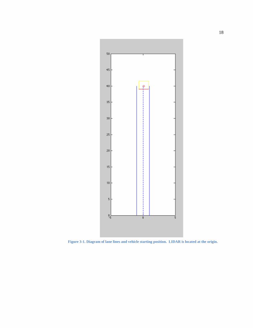
The lane that the vehicle will navigate will be completely straight extending in the y-

direction, 40 meters long, and 2 meters wide, centered about the origin and the location of the

17

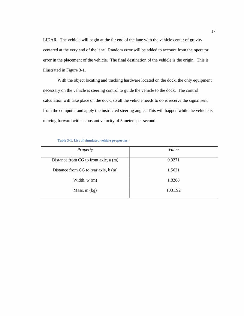
LIDAR. The vehicle will begin at the far end of the lane with the vehicle center of gravity

centered at the very end of the lane. Random error will be added to account from the operator

error in the placement of the vehicle. The final destination of the vehicle is the origin. This is

illustrated in Figure 3-1.

With the object locating and tracking hardware located on the dock, the only equipment

necessary on the vehicle is steering control to guide the vehicle to the dock. The control

calculation will take place on the dock, so all the vehicle needs to do is receive the signal sent

from the computer and apply the instructed steering angle. This will happen while the vehicle is

moving forward with a constant velocity of 5 meters per second.

Table 3-1. List of simulated vehicle properties.

Property Value

Distance from CG to front axle, a (m) 0.9271

Distance from CG to rear axle, b (m) 1.5621

Width, w (m) 1.8288

Mass, m (kg) 1031.92

18

Figure 3-1. Diagram of lane lines and vehicle starting position. LIDAR is located at the origin.

19

Chapter 4

Lane Following and Vehicle Control

Once the vehicle is placed in the desired starting position, it must begin following its path

to reach the dock. The simulation determines a path from the location of the lane markers and

enables the vehicle to follow that path until completion. This chapter details how the simulation

goes about controlling the vehicle through the docking process.

4.1 Lane Detection

Usually, before a path is planned, the lane lines must be found. This process would

involve taking image data from a camera, creating an edge distribution function, and applying a

Hough transformation to create smooth lines. However, in this simulation, this process is not

necessary. Instead, the location of the lane lines is already known by the x,y - coordinates of the

constituent points. More specifically, the lines are also known to be perfectly straight. Once the

lines are known, a desired vehicle path can be planned directly in between them for the vehicle

center of gravity to follow.

4.2 Vehicle Control

Due to the presence of a random error at the initial placement, the vehicle will not start

exactly at the beginning of the path, nor will it be pointed directly at the final destination. For

this reason, a control system must be in place to take position and orientation feedback to guide

the vehicle along the desired path. This control structure is shown in Figure 4-1.

20

4.2.1 Vehicle Model

Because of the complex nature of many of the systems inside a vehicle, many variables

go into determining vehicle response from a given steering input. To simplify this calculation,

assumptions are made to provide a workable vehicle model.

First, a bicycle model will be used with three degrees of freedom: longitudinal, lateral,

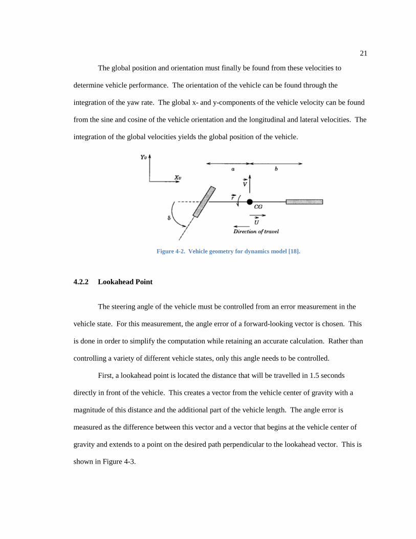
and yaw. A diagram of the model is shown in Figure 4-2. The longitudinal velocity of the

vehicle will be constant throughout the path for this system. Using Ackermann steering

geometry, the yaw rate can be found with relation to steering angle and forward velocity as

follows.

𝑅 =𝐿𝛿

𝑟 =𝑈𝑅

Also, the vehicle will be assumed to operating at low speeds. This is the case in order to

allow for more assured object tracking and thus increased safety. At such low speeds, the lateral

velocity in the vehicle's frame of reference is zero because there is no slip angle. This removes

the necessity for more complex calculations that slip-based dynamics requires.

Figure 4-1. Control system diagram for lane following

21

The global position and orientation must finally be found from these velocities to

determine vehicle performance. The orientation of the vehicle can be found through the

integration of the yaw rate. The global x- and y-components of the vehicle velocity can be found

from the sine and cosine of the vehicle orientation and the longitudinal and lateral velocities. The

integration of the global velocities yields the global position of the vehicle.

4.2.2 Lookahead Point

The steering angle of the vehicle must be controlled from an error measurement in the

vehicle state. For this measurement, the angle error of a forward-looking vector is chosen. This

is done in order to simplify the computation while retaining an accurate calculation. Rather than

controlling a variety of different vehicle states, only this angle needs to be controlled.

First, a lookahead point is located the distance that will be travelled in 1.5 seconds

directly in front of the vehicle. This creates a vector from the vehicle center of gravity with a

magnitude of this distance and the additional part of the vehicle length. The angle error is

measured as the difference between this vector and a vector that begins at the vehicle center of

gravity and extends to a point on the desired path perpendicular to the lookahead vector. This is

shown in Figure 4-3.

Figure 4-2. Vehicle geometry for dynamics model [18].

22

This angle error can be using various other state errors. Since the point on the path is

perpendicular to the lookahead vector it creates a right triangle. Using trigonometric functions,

the error angle can be found from the distance error and the vehicle orientation. The calculations

are shown below.

sin𝜃 =𝑦𝑒𝑟𝑟𝑜𝑟𝑑 + 𝑎

− 𝜙

For small angles, 𝜃 = 1𝑑+𝑎

𝑦 − 𝜙

4.2.3 PD Control

A PD controller is added in order to control the steering angle in relation to the angle

error. A hand-tuned value of 3 radians of steering per degree of angle error is chosen for the

proportional gain. This gain was chosen as it results in a response that is stable and has no

Figure 4-3. Geometry of lookahead point [18].

23

overshoot; however, it takes a significant amount of time to reach the steady state value. This is

not a significant problem, however, as the vehicle only needs to stay in its lane. So, minor

differences in the path are not important. However, derivative control is added to improve this

performance. A derivative gain of 0.87 radians of steering per degrees/sec of error velocity is

chosen through experimentation to produce the shortest rise time while still remaining stable.

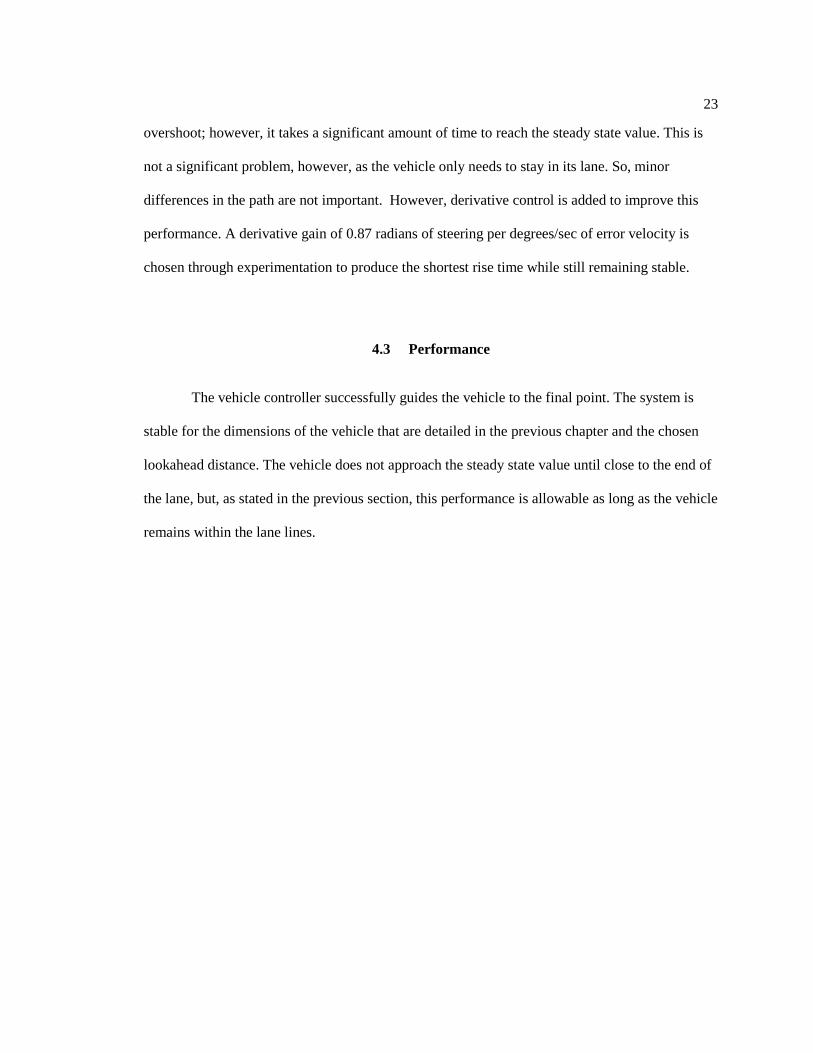
4.3 Performance

The vehicle controller successfully guides the vehicle to the final point. The system is

stable for the dimensions of the vehicle that are detailed in the previous chapter and the chosen

lookahead distance. The vehicle does not approach the steady state value until close to the end of

the lane, but, as stated in the previous section, this performance is allowable as long as the vehicle

remains within the lane lines.

24

Figure 4-4. Vehicle location at 3 different times during the lane following process.

Left is the starting point with the path planned. Middle is the vehicle after 3 seconds. Right is the vehicle after 6 seconds.

25

Chapter 5

Object Detection

In order for the vehicle to reach the dock without collision, it must first detect objects that

may be in the path. The simulation includes a virtual LIDAR and a system that tracks objects

using this LIDAR data. These chapter details the functionality of these subsystems as well as the

results.

5.1 LIDAR Simulation

To generate functional LIDAR data that can be used in the object tracking algorithms, a

simulated LIDAR must be created. This simulation first creates a 2-dimensional grid throughout

the view of the sensor. Each square in this grid is 10 cm wide to account for the limited

resolution of the LIDAR that is being represented. Next, a strike matrix is created for the device

that specifies the order that grid squares should be observed. This also reduces run time since it

does not need to read squares that are behind squares that are filled and can eliminate repeated

squares.

Each object that may be in the field of view is first represented by an occupancy map.

Object position and size are taken into account so the map contains a series of zeros and ones that

show where objects are. The strike matrix structure can be executed using the occupancy map to

produce range data similar to what would be produced by a LIDAR once the empty rays are given

the maximum values. The known object positions and orientations will no longer be used and

will be replaced by this LIDAR data.

26

5.2 Object Tracking

The LIDAR data must be processed in order to track the objects in the environment. This

process requires the separation of the foreground and background, grouping of the data points

into objects, recognizing the object motion between frames, and the prediction of future motion.

The simulation used for this is based on the program developed by Guo for the tracking of

multiple pedestrians and vehicles at an intersection [1].

5.2.1 Pre-processing

The first step in processing the data is distinguishing between foreground and background

using the technique of background subtraction. First, any data points corresponding to the

LIDAR's maximum functional range can be removed since it provides no usable information.

Next, permanent fixtures in the field of view must be determined in order to remove

them. A voting system is employed to locate these background features over several initial

frames. When the LIDAR detects an object at a specific location that grid receives a vote, and

after several frames, the grids with the most votes will be known to be stationary. Since the

environment will be entirely open for this simulation, any grid squares not filled by an object will

be empty. This makes this technique excessive, but for further testing with permanent background

objects, it will be necessary to include.

5.2.2 Segmentation

With only the foreground data points remaining, they must be segmented to group them

into complete objects. To do so, a DBSCAN algorithm is utilized to group points based on their

ability to be density-connected since it eliminates noise better than an adaptive distance model.

27

Since the environment is usually open around a loading dock area, occlusions will be rare.

However, the segmentation process should still account for the possibility that an object is at least

partially occluded by another object in the field of view. If the distances of the rays immediately

before and after the segment endpoints is smaller than that of the endpoint, the segment is

extended for the next 5 rays to enable the possibility of connecting to the part of the object that

may be on the other side of the occlusion.

The next step is to classify each object based on its distinct features. The first criterion is

size, where objects over 80 cm will be assumed to be vehicles and anything smaller will be

people. Vehicles will be able to be fitted with an L-shape or straight line that approximates their

shape. This can be done by first finding the corner of the vehicle then fitting lines to the two

associated sides. The corners can be used as feature points for further processing.

5.2.3 Data Association

In order to follow each object, the same object must be located in consecutive frames and

associated. This will be done with a Greediest Nearest Neighbor algorithm. As shown in Chapter

2, this associates the object in later frames that is closest to the location in the original frame. The

Mahalanobis distance is used in place of Euclidean distance to account for direction of travel.

Feature points are used in the association to reduce the necessary computation. To account for

possible errors, if an object moves in a manner that is highly unlikely, the object is stored until a

successful association is found.

28

5.3 Performance

The LIDAR simulation produces a final set of data that is very similar to what would be

produced by an actual LIDAR. The majority of points correspond to the maximum range of the

device, which is to be expected in the open environment. The objects appear as cutouts in an

otherwise smooth semicircle. The only thing that the simulation is lacking is noise points. This

is not a problem, as it merely removes the necessity for a filtering step. An example of a

simulated LIDAR scan is shown in Figure 5-1.

The tracking algorithm is able to successfully locate any objects that are within the

LIDAR’s field of view. It is able to segment the data and classify objects as either people or

vehicles. Where the algorithm lacks, however, is in the tracking of the objects. The data

association step can be inconsistent, and segments in new frames are often considered new

objects rather than the previously moving object. This is especially noticeable at high velocities

Figure 5-1. An example of a simulated LIDAR scan

29

and accelerations as well as during and after occlusions. An example of a successful tracking is

shown in Figure 5-2.

Figure 5-2. Sample tracking of vehicle and two objects

-8000 -6000 -4000 -2000 0 2000 4000 6000 80000

1000

2000

3000

4000

5000

6000

7000

8000

30

Chapter 6

Collision Avoidance

With the known position and motion of any obstacles that may be in the field of view,

measures can be taken to avoid collision. Once the distance between the vehicle and the object is

deemed to be too close, a decision must be made as to whether to apply the brakes or attempt an

evasive turn. This chapter details how this system is applied to the vehicle control simulation

with the information from the object tracking.

6.1 Proximity Measurement

Before any action must be taken, a possible collision must be detected. Each time step,

the distance between the vehicle and the nearest feature point on each object is calculated. The

vehicle will take action if this value is within a 3 m range, which is reserved for when the object

is only first detected when it is already quite close. Otherwise, the motion model will be used to

predict whether or not the vehicle and the object will be within a dangerous distance of each other

in the near future. The past 5 frames are used to interpolate the measured position data to predict

a possible path for the object. The motion of the object will also determine the maneuver the

vehicle performs if evasive action is necessary.

31

6.2 Braking

The first possible course of action to take is to apply the brakes. This technique will be

applied in the case of an object that is or will be in front of the vehicle on or near its planned path.

This is an ideal course of action since, throughout the maneuver, the vehicle remains entirely in

its lane. This is useful if similar docking processes are to be conducted simultaneously in close

proximity.

Before the vehicle attempts to brake to avoid an impending collision, it must be known if

the vehicle is able to stop in a short enough distance. To do this, a minimum braking distance is

calculated. For this calculation, a simplistic friction model is used, assuming the brakes are

completely locked. This requires a known vehicle weight and coefficient of friction between the

tires and asphalt. Using these values, the calculations proceed as follows.

𝐹 = −𝜇𝑁

𝑚𝑎 = −𝜇𝑚𝑔

𝑎 = −𝜇𝑔

2𝑎𝑑 = 𝑈𝑓2 − 𝑈𝑜2

𝑑 =𝑈2

2𝜇𝑔

If the potential distance between the vehicle and the object is greater than this minimum

stopping distance, then less acceleration can be applied as long as it still provides a sufficient

safety tolerance.

𝑎 = −𝑈2

2𝑑

If the vehicle to object distance does not meet this minimum requirement, other

avoidance maneuvers must be performed.

32

6.3 Turning

The next option that is used to avoid a collision is to turn the vehicle away from the

approaching object. For this, a turn with a constant radius will be used. The feature points taken

from the object tracking subsystem are used to identify the corners of the object that the vehicle

must successfully avoid. The turn radius necessary to clear the corner is found using the

following calculations. The angle difference is found using the tangent of the triangle formed by

the x-difference and y-difference between the vehicle CG and the desired point. The radius is

found using the perpendicular bisector of the segment connecting the two points. The maximum

steering angle allowed by the vehicle is 20 degrees.

tan𝜃 =𝑥𝑦

𝜃 = tan−1𝑥𝑦

sin𝜃 =12�𝑥

2 + 𝑦2

𝑅

𝑅 =�𝑥2 + 𝑦2

sin(tan−1 𝑥𝑦)

The direction the vehicle must turn in order to have the highest probability of avoiding a

collision is then determined. The first consideration is the presence of objects in close proximity

to the sides of the vehicle. In this case, the direction where there is the most open space is

chosen. If both sides are open, the vehicle will proceed in the direction opposite of the current

location of the approaching object.

33

Chapter 7

Experimental Results

Multiple tests are performed on the finished simulation to determine how successful it is.

These tests include many different paths and speeds for the object, as well as the introduction of

multiple simultaneous objects. This chapter explains the results of the simulation through each of

these tests, including the failures.

7.1 Results

7.1.1 Stationary Object

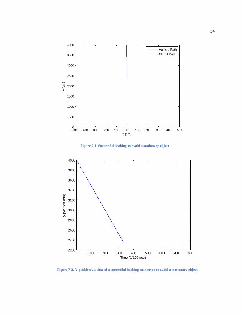
The first test involves a stationary object in the vehicle environment. The object is placed

slightly off the center of the lane, halfway between the starting point and the dock. The object is

successfully located using the LIDAR simulation, aided by the fact that the object is not moving.

Since the object is directly in the path of the vehicle, once the vehicle enters the range at which

action is necessary, a braking maneuver is executed. Since the object is seen so far in advance,

the maximum deceleration is not necessary, so the vehicle comes to a comfortable stop.

34

Figure 7-1. Successful braking to avoid a stationary object

Figure 7-2. Y-position vs. time of a successful braking maneuver to avoid a stationary object

-500 -400 -300 -200 -100 0 100 200 300 400 5000

500

1000

1500

2000

2500

3000

3500

4000

x (cm)

y (c

m)

Vehicle PathObject Path

0 100 200 300 400 500 600 700 8002200

2400

2600

2800

3000

3200

3400

3600

3800

4000

Time (1/100 sec)

y po

sitio

n (c

m)

35

7.1.2 Object with Constant Velocity

Now, the object is given a low, constant velocity. The object is once again successfully

tracked throughout its trajectory. The path is predicted very accurately due to the constant

velocity. In cases where the object path intersects that of the vehicle, the system identifies the

impending collision well in advance. The vehicle brakes similar to the way it did in the previous

test. If the object never approaches the vehicle, the vehicle proceeds along its path without

adjusting its route.

If the object is moving with high velocities, however, the vehicle is not always able to

react. In this case, the object is not tracked as well, and a definite location is not found at some

time intervals. The motion model partially covers this problem, but many consecutive missing

points result in an inaccurate prediction. When this happens, the vehicle either detects the

possible collision late and turns away or collides with the object.

Figure 7-3. Successful braking to avoid an object with constant velocity

-1500 -1000 -500 0 500 1000500

1000

1500

2000

2500

3000

3500

4000

x (cm)

y (c

m)

Vehicle PathObject Path

36

Figure 7-4. Y-position vs. time of vehicle for a successful braking maneuver to avoid a constant velocity object

7.1.3 Object with Acceleration

When a constant acceleration is added to the moving object, the results are quite similar

to the previous constant velocity test. If the velocity and acceleration are sufficiently low, the

object will be tracked well, and the vehicle reacts and brakes comfortably with plenty of time to

spare. However, if these values are raised significantly, the objects are not tracked as well. With

the addition of acceleration, if there are multiple consecutive frames that the object is not tracked,

the path prediction suffers, resulting in more collisions.

0 100 200 300 400 500 600 700 8002800

3000

3200

3400

3600

3800

4000

Time (1/100 sec)

y po

sitio

n (c

m)

37

7.1.4 Multiple Objects

As a final test, a second object is added. One object crosses the vehicles path while the

other remains a significant distance away. In this case, the vehicle reacts to the incoming object

as it has in previous tests, depending on the manner of the motion. The only effect the second

object has is influencing the vehicle to turn away from the object if it is forced to make a

maneuver around the other object.

7.2 Failure Analysis

Though the system performed as expected in a majority of test situations, there we certain

cases where the vehicle was unable to avoid a collision. These cases are limited to those with

objects with especially high velocity or acceleration values. The error can be traced to the data

association step of the object tracking system. With errors in this step, the object is not always

followed, and when it is, it is often stored as a new object. To resolve the problem, a more

advanced association algorithm may be used such as JPDA or MHT, as discussed in Chapter 2.

38

Chapter 8

Conclusion

With the increased desire for vehicle automation, safety systems are crucial to go along

with the vehicle control systems. Using a dock-mounted LIDAR, objects near the vehicle can be

located and tracked as the vehicle performs a docking maneuver. It is important that the vehicle

can then take evasive actions if a dangerous object is present.

This thesis has shown, using a simulation, that the vehicle can be controlled using the

feedback from position error and orientation to find a single lookahead point angle error to

control. With the addition of a PD controller, the vehicle can navigate a straight path. Using a

simulated LIDAR, range data can be successfully produced from a map that contains multiple

objects. This data can be segmented and classified to find the location and type of the objects in

the field of view. The objects can then be tracked using a nearest neighbor filter with a small

degree of success. With this information, the vehicle can make avoidance maneuvers based on

the location and velocity of the objects. The success of the collision avoidance measures is

entirely dependent on the accuracy of the object tracking. However, accurate object position data

is often all that is necessary for the vehicle to avoid the object.

This leaves a lot of room for future work. The lane that leads to the dock can be changed

to an arbitrary curve for the vehicle to follow. An improved object tracking subsystem can be

achieved through the application of more advanced data association techniques. Collision

avoidance can be improved by employing dynamic turning that includes braking in the turn.

Finally, the system can be applied to a physical prototype to observe the practical effectiveness.

39

BIBLIOGRAPHY

[1] Gou, Mengran. Lidar-based Multi-object Tracking System with Dynamic Modeling. Thesis. Pennsylvania State University, 2012. N.p.: n.p., n.d. [2] M. Piccardi, “Background subtraction techniques: A review," IEEE International Conference on Systems, Man and Cybernetics, 2004, pp. 3099-3104 [3] A. Fod, A. Howard, and M. J. Mataric, “Laser-based people tracking," IEEE International Conference on Robotics and Automation, Washington DC, May, 2002, pp. 3024-3029 [4] A. Elfes, “Occupancy grids : a probabilistic framework for robot percEpetion and navigation," PhD thesis, Carnegie Mellon University, 1989 [5] T. D. Vu, O. Aycard, and N. Appenrodt, “Online localization and mapping with moving object tracking in dynamic outdoor environments," IEEE Intelligent Vehicles Symposium, Istanbul, Turkey, June 2007 [6] J. Sparbert, K. Dietmayer, and D. Streller, “Lane detection and street type classification using laser range images," IEEE Intelligent Transportation System Conference, Oakland, CA, USA, Aug. 2001 [7] A. Mendes, L. C. Bento, and U. Nunes, “Multi-target detection and tracking with a laser-scanner," IEEE Intelligent Vehicles Symposium, Parma, Italy, June 2004 [8] M. Ester, H. Kriegel, J. Sander, X. Xu, “A density-based algorithm for discovering clusters in large spatial databases with noise," proc. 2nd Int. Conf. on Knowledge Discovery and Data Mining, Portland, OR, USA, 1996, pp. 226 [9] L. Zhao and C. Thorpe, “Qualitative and quantitative car tracking from a range image sequence," CVPR, Santa Barbara, CA, June 1998, pp. 496-501 [10] T. Deselaers, D. Keysers, R. Paredes, E. Vidal, and H. Ney, “Local representations for multi-object recognition," DAGM 2003, Pattern Recognition, 25th DAGM Symp, pp. 305312, September 2003 [11] S. Thrun, “Particle Filters in Robotics," The Eighteenth Conference on Uncertainty in Artificial Intelligence, San Francisco, CA, USA, 2002 [12] D. Schulz, W. Burgard, D. Fox, and A. B. Cremers “Tracking multiple moving targets with a mobile robot using particle filters and statistical data association," IEEE International Conference on Robotics and Automation, Seoul, Korea, 2001, pp. 1665-1670 [13] A. Petrovskaya and S. Thrun, “Model based vehicle tracking in urban environments," IEEE

40

International Conference on Robotics and Automation, Workshop on Safe Navigation, Vol. 1, 2009, pp. 1-8 [14] D. Schulz, W. Burgard, D. Fox, and A. B. Cremers, “People tracking with a mobile robot using sample-based joint probabilistic data association filters," The International Journal of Robotics Research, Vol. 22, No. 2, 2003, pp.99-116 [15] D. Streller, K. Furstenberg, and K. Dietmayer, “Vehicle and object models for robust tracking in traffic scenes using laser range images," IEEE 5th International Conference on Intelligent Transportation System, Singapore, Sept. 2002 [16] C. C. Wang, C. Thorpe, M. Hebert, S. Thrun, and H. D. Whyte, “Simultaneous localization, mapping and moving object tracking," The International Journal of Robotics Research, Vol. 26, No. 9, Sept. 2007, pp.889-916 [17] Jung, C.R.; Kelber, C.R., "A robust linear-parabolic model for lane following," Computer Graphics and Image Processing, 2004. Proceedings. 17th Brazilian Symposium on , vol., no., pp.72,79, 17-20 Oct. 2004 [18] Unyelioglu, K.A.; Hatipoglu, C.; Ozguner, U., "Design and stability analysis of a lane following controller," Control Systems Technology, IEEE Transactions on , vol.5, no.1, pp.127,134, Jan 1996 [19] Jung, Cláudio Rosito, and Christian Roberto Kelber. "Lane following and Lane Departure Using a Linear-parabolic Model." Image and Vision Computing 23.13 (2005): 1192-202. [20] Fox, D.; Burgard, W.; Thrun, S., "The dynamic window approach to collision avoidance," Robotics & Automation Magazine, IEEE , vol.4, no.1, pp.23-33, Mar 1997 [21] Khatib, O. "Real-Time Obstacle Avoidance for Manipulators and Mobile Robots." The International Journal of Robotics Research 5.1 (1986): 90-98 [22] Vahidi, A., and A. Eskandarian. "Research Advances in Intelligent Collision Avoidance and Adaptive Cruise Control." IEEE Transactions on Intelligent Transportation Systems 4.3 (2003): 143-53.

ACADEMIC VITA

Kyle Reigh kmr5339@psu.edu

Campus Address Permanent Address 421 E. Beaver Ave, Apt. B5 119 Penns Grant Drive State College, PA 16801 Morrisville, PA 19067

Professional Profile

• Skilled design engineer with experience that includes project manager and primary concept generator in the design of a product for a local business

• Experienced research assistant with skills in communication and interpersonal skills, as well as leadership and problem-solving

• Specialization in mechatronics and automation, including control systems Education Bachelor of Science in Mechanical Engineering, The Pennsylvania State University, University Park, PA, Schreyer Honors College, Anticipated Graduation: August 2013, Specialization: Mechatronics. Academic Honors and Awards

• Schreyer Honors College Academic Excellence Scholarship • Charles Henry Berle Memorial Scholarship • Paul Morrow Endowed Scholarship in the College of Engineering • Harding Lewis Memorial Scholarship • President’s Freshman Award • National Society of Collegiate Scholars, member • Dean’s List: 8 semesters

Research Experience Research Assistant The Pennsylvania State University (2011)

• Worked in the Larson Transportation Institute (LTI) on designing objects to stop vehicles moving at high speeds

• Collaborated in the design and execution of 9 full-scale crash tests • Analyzed high speed footage and recreated the impacts using Photron and

MATLAB • Participated in friction workshop to test and calibrate devices that measure the

coefficients of friction of various road surfaces

Professional Affiliations

• Phi Beta Lambda, Professional Business Fraternity, Pledge Class President and Parliamentarian

• American Society of Mechanical Engineers, member • Penn State Dance MaraTHON, Atlas, member

Skills

• C++, Python, MATLAB, Arduino, SolidWorks, Photron, Microsoft Office 97-2013

• Spanish - four semesters • Machining, welding