the pennsylvania state university department of aerospace
TRANSCRIPT

The Pennsylvania State University
The Graduate School
Department of Aerospace Engineering
ROTORCRAFT PERFORMANCE ENHANCEMENTS
DUE TO A LOWER-SURFACE MINATURE EFFECTOR
A Thesis in
Aerospace Engineering
by
Robert L. Roedts II
2008 Robert L. Roedts II
Submitted in Partial Fulfillment of the Requirements
for the Degree of
Master of Science
August 2008

ii
The thesis of Robert L. Roedts II was reviewed and approved* by the following:
Mark D. Maughmer Professor of Aerospace Engineering Thesis Advisor
Barnes W. McCormick Boeing Professor Emeritus of Aerospace Engineering
George A. Lesieutre Professor of Aerospace Engineering Head of the Department of Aerospace Engineering
*Signatures are on file in the Graduate School

iii
ABSTRACT
Although the application of advanced structures and intelligent control systems on
helicopters has seen a dramatic increase over the past two decades, the overall performance of
helicopters, relative to fixed-wing aircraft, is somewhat stagnant. This is due to many factors, one of
them being the lack of innovative aerodynamic devices that can operate in the unique environment
of a rotor. Research over the past 20 years has shown that in order to have a performance increase
with the rotor, it must adapt, or “morph,” to the changing environment around the azimuth. One
method that is being researched is the use of Miniature Trailing-Edge Effectors (MiTEs) on the
blades of the rotor. MiTEs are an extension of the passive high-lift device, the Gurney flap. Gurney
flaps are small flat plates, between 0.5 to 5 percent chord, fitted perpendicular to the airfoil surface at
or near the trailing edge of a wing or rotor blade. A MiTE is an active Gurney flap, which can be
used to actively control the lift and moment distribution on a rotor blade. MiTEs also have the
advantage of having very low actuator loads compared to those of traditional trailing-edge flaps.
Experimental and validated computational fluid dynamics research has been done on MiTEs and an
unsteady aerodynamic model was created for MiTEs placed at the trailing edge. In this work, this
model has been modified to account for a MiTE placed at the trailing edge up to the 85 percent
chord position. This aerodynamic model has also been incorporated into a rotor performance code
to predict the effect of MiTEs on rotor performance and explore their ability to extend the flight
envelope of the RAH-66 Comanche. The maximum velocity of Comanche was shown to have the
potential increase of 20 percent with the increased use of transonic airfoils as facilitated through the
use of MiTEs on the outboard section of the rotor blades. Investigations were also made on
increasing the service ceiling of the Comanche, which showed a potential improvement of 8 percent
with the use of MiTEs.

iv
TABLE OF CONTENTS
LIST OF FIGURES...................................................................................................................................vi
LIST OF TABLES .....................................................................................................................................x
ACKNOWLEDGEMENTS....................................................................................................................xi
Chapter 1 Introduction.............................................................................................................................1
1.1 Description of the Rotor Environment...................................................................................2 1.1.1 Region I: Compressibility on Advancing Blade..........................................................4 1.1.2 Region II: Retreating Blade Stall ...................................................................................5 1.1.3 Region III: Hover............................................................................................................6
1.2 Airfoil Design...............................................................................................................................6 1.2.1 Initial and First Generation Airfoils .............................................................................6 1.2.2 Modern Airfoils ...............................................................................................................7
1.3 Flow Control ................................................................................................................................9 1.3.1 Boundary-Layer Control ................................................................................................9 1.3.2 Zero-Mass Flow Synthetic Jets .....................................................................................10
1.4 Miniature Trailing-Edge Effectors............................................................................................11 1.4.1 Background ......................................................................................................................11 1.4.2 Rotor Applications..........................................................................................................14
1.4.2.1 Individual Blade Control....................................................................................15 1.4.2.2 Rotor Performance Enhancement ...................................................................15 1.4.2.3 Other Potential Applications of MiTEs ..........................................................17
Chapter 2 Experimental and CFD Investigations ................................................................................18
2.1 Static Wind Tunnel Testing .......................................................................................................18 2.1.1 Wind Tunnel Description and Airfoil Model .............................................................18 2.1.2 Experimental Results ......................................................................................................20
2.2 NASA Ames Dynamic Wind Tunnel Testing ........................................................................27 2.2.1 Wind Tunnel Description and Airfoil Model .............................................................28 2.2.2 Experimental Results ......................................................................................................31
2.3 Wind Tunnel Experimental Conclusions ................................................................................35 2.4 CFD Investigations .....................................................................................................................36
2.4.1 Gurney Flapped Airfoils.................................................................................................36 2.4.1.1 VR-12: 0.01c Gurney Flap located at 1.0c ......................................................37 2.4.1.2 VR-15: 0.01c Gurney Flap located at 1.0c ......................................................38
2.4.2 Dynamic MiTE CFD Results........................................................................................39 2.4.2.1 VR-12 Airfoil: 0.01c height MiTE at 1.0c .......................................................40 2.4.2.2 VR-12 Airfoil: 0.02c height MiTE at 0.9c .......................................................43
2.5 CFD Conclusions ........................................................................................................................48
Chapter 3 Aerodynamic Modeling..........................................................................................................49
3.1 Gurney Flap Effects....................................................................................................................49 3.2 Dynamic Stall ...............................................................................................................................51

v
3.2.1 Leishman-Beddoes Dynamic Stall Model ...................................................................53 3.2.1.1 Oscillating Airfoil with Attached Flow............................................................53 3.2.1.2 Oscillating Airfoil In Dynamic Stall .................................................................54
3.3 Unsteady Flapping Model ..........................................................................................................58 3.3.1 Indicial Response of MiTEs ..........................................................................................59 3.3.2 Modified Hariharan-Leishman Unsteady Flapped Airfoil Model ...........................60
3.3.2.1 Modified Hariharan-Leishman Model Normal Force...................................60 3.3.2.2 Modified Hariharan-Leishman Model Pitching Moment .............................62 3.3.2.3 Modified Hariharan-Leishman Model Drag Force........................................63
3.3.3 Additional Effects from Upstream MiTEs .................................................................64 3.3.4 Parameters of Modified Hariharan-Leishman Model................................................66 3.3.5 Results of the Modified Hariharan-Leishman Model................................................66
3.3.5.1 Trailing Edge MiTE............................................................................................67 3.3.5.2 Upstream MiTE...................................................................................................71
3.4 MiTE Aerodynamic Model ........................................................................................................74 3.5 Summary .......................................................................................................................................77
Chapter 4 MiTE Rotor Performance .....................................................................................................78
4.1 ROTOR Program........................................................................................................................78 4.1.1 Generation of Airfoil Data Tables................................................................................79 4.1.2 Aerodynamic Models......................................................................................................80
4.1.2.1 Oscillating Airfoil Model....................................................................................80 4.1.2.2 Oscillating MiTE Model ....................................................................................81
4.1.3 MiTE Deployment Scheme...........................................................................................81 4.2 Rotor Performance Analysis......................................................................................................83
4.2.1 Importance of Unsteady Modeling...............................................................................84 4.2.2 Pitching Moment Concern ............................................................................................86 4.2.3 Forward Speed Performance.........................................................................................87 4.2.4 Maximum Altitude Performance ..................................................................................88
4.3 Advanced Designs.......................................................................................................................89 4.3.1 Rotors Designed with MiTEs........................................................................................90 4.3.2 Deployment Schemes .....................................................................................................90
4.4 Summary .......................................................................................................................................91
Chapter 5 Conclusion................................................................................................................................92
5.1 Summary of Results ....................................................................................................................92 5.1.1 Wind Tunnel Experiments ............................................................................................92 5.1.2 CFD Investigations .........................................................................................................93 5.1.3 Aerodynamic Modeling ..................................................................................................93 5.1.4 MiTE Rotor Performance..............................................................................................94
5.2 Conclusions ..................................................................................................................................94
List of References .......................................................................................................................................95

vi
LIST OF FIGURES
Figure 1-1: Rotor Operating Environment.[2] .......................................................................................3
Figure 1-2: The rotor disk showing the areas of compressibility and reverse flow.[1] ....................4
Figure 1-3: The weighted quasi-steady aerodynamic requirements for the blades are such that different airfoils must be employed at different radial stations.[8] ............................................7
Figure 1-4: A selection of rotorcraft airfoils through the generations.[8]..........................................8
Figure 1-5: Historical trends in rotor blade loading.[8] ........................................................................9
Figure 1-6: Schematic of a synthetic jet actuator (SJA).[8]...................................................................10
Figure 1-7: Concept of MiTE[13].............................................................................................................11
Figure 1-8: Liebeck’s hypothesized flow structure around MiTE.[18] ...............................................12
Figure 1-9: Summary of 1 percent chord height Gurney flap effects to the maximum lift for several airfoils at varying flow conditions.[26] ..............................................................................14
Figure 1-10: Comparison between baseline and MiTE rotor performance in level forward flight with variations in the gross weight calculated using the dynamic stall model and without an optimal MiTE deployment schedule.[26] .................................................................16
Figure 2-1: The 3.25' x 4.75' cross section of the S903 airfoil placed in the Penn State Low-Turbulence, Low-Speed Wind Tunnel. ..........................................................................................19
Figure 2-2: The S903 airfoil compared to the VR-12 airfoil ................................................................20
Figure 2-3: Pressure distributions at cl = 0.7 with and without Gurney flaps...................................20
Figure 2-4: Pressure distributions at cl.max with and without Gurney flaps .........................................21
Figure 2-5: Aerodynamic characteristics with varying Gurney flap heights, at the trailing edge ...23
Figure 2-6: Aerodynamic characteristics with varying Gurney flap chord-wise locations ..............24
Figure 2-7: Aerodynamic characteristics with natural transition and transition fixed at 0.02c on the upper surface and 0.05c on the lower ................................................................................25
Figure 2-8: ∆cl,max with varying Gurney flap heights and chordwise locations ..................................25
Figure 2-9: Comparison of the aerodynamic characteristics with a 0.01c high Gurney flap located at the trailing edge on the upper and lower surfaces......................................................26
Figure 2-10: Comparison of plain flap and MiTE.................................................................................27
Figure 2-11: Compressible Dynamic Stall Facility at NASA Ames ....................................................29

vii
Figure 2-12: Comparison of the trailing edge profiles of the designed VR-12 airfoil to that fabricated for experiments................................................................................................................30
Figure 2-13: Comparison of the static polars of the designed VR-12 airfoil to that fabricated for experiments, as calculated by MSES at M=0.4, Re =1.4e6 ..................................................30
Figure 2-14: Comparison of the pressure distribution the designed VR-12 airfoil to that fabricated for experiments................................................................................................................31
Figure 2-15: The quasi-steady experimental results comparing the VR-12 baseline and with a 0.0135c height Gurney flap through stall at M=0.3. (a) lift and drag (b) Gurney flap effects of lift and drag .......................................................................................................................32
Figure 2-16: Comparison of the lift for the VR-12 baseline airfoil and with a 0.0135c height Gurney flap in dynamic stall at a reduced frequency of 0.05......................................................33
Figure 2-17: Comparison of the drag for the VR-12 baseline airfoil and with a 0.0135c height Gurney flap in dynamic stall at a reduced frequency of 0.05......................................................33
Figure 2-18: Comparison of the drag polars for the VR-12 baseline airfoil and with a 0.0135c height Gurney flap in dynamic stall at a reduced frequency of 0.05..........................................34
Figure 2-19: Comparison of the pitching moment for the VR-12 baseline airfoil and with a 0.0135c height Gurney flap in dynamic stall at a reduced frequency of 0.05...........................35
Figure 2-20: Gurney flap effects with Mach number variations for the VR-12 airfoil (a)lift increment (b) drag increment (c) moment increment..................................................................37
Figure 2-21: Gurney flap effects with Mach number variations for the VR-15 airfoil (a)lift increment (b) drag increment (c) moment increment..................................................................39
Figure 2-22: Force and moment for the sinusoidal deployment of a 0.01c MiTE located 1.0c, compared to static wind-tunnel data. (a) ω=5Hz (k=0.14) (b) ω=20Hz (k=0.54) ................41
Figure 2-23: Effect of the lift with changes in deployment frequency for a MiTE located at 1.0c, at various free-stream conditions, and compared to incompressible theories................42
Figure 2-24: Effect of the drag and pitching moment with changes in deployment frequency of a MiTE located at 1.0c for various free-stream conditions....................................................42
Figure 2-25: Instantaneous streamlines calculated in OVERFLOW2 for a 0.02c height MiTE positioned at 0.9c, deploying at w=5Hz (k=0.14) .......................................................................43
Figure 2-26: Force and moment for the sinusoidal deployment of a 0.02c MiTE located 0.9c, compared to static wind-tunnel data. (a) ω=5Hz (k=0.14) (b) ω=20Hz (k=0.54) .................45
Figure 2-27: Effect of the lift with changes in deployment frequency of a MiTE located at 0.9c for various free-stream conditions compared to incompressible theories .......................46
Figure 2-28: Drag effect of MiTE located at 0.9c with changes in the deployment frequency for various free-stream conditions ..................................................................................................47

viii
Figure 2-29: Pitching Moment effect of MiTE located at 0.9c with changes in the deployment frequency for various free-stream conditions .........................................................47
Figure 3-1: Example airfoil data sets modified to predict the effects of a Gurney flap at various Mach numbers......................................................................................................................51
Figure 3-2: Force, moment, and flow characteristics of dynamic stall. [1] ........................................52
Figure 3-3: Results of Leishman-Beddoes dynamic stall model for the VR-12 airfoil with and without a Gurney flap compared with wind tunnel and CFD results. [26] .............................58
Figure 3-4: Indicial Responses at various Mach numbers calculated by CFD [26] ..........................59
Figure 3-5: Comparisons between CFD and modified H-L unsteady flapping model for M=0.1, α=0 deg, k=0.14 (a) lift (b) drag (c) moment [26] ..........................................................67
Figure 3-6: Comparisons between CFD and modified H-L unsteady flapping model for M=0.1, α=0 deg, k=0.56 (a) lift (b) drag (c) moment [26] ...........................................................68
Figure 3-7: Comparisons between CFD and modified H-L unsteady flapping model for M=0.3, α=10 deg, k=0.2 (a) lift (b) drag (c) moment [26] ...........................................................69
Figure 3-8: Comparisons between CFD and modified H-L unsteady flapping model for M=0.6, α=0 deg, k=0.5 (a) lift (b) drag (c) moment [26]..............................................................70
Figure 3-9: Magnitude and phase lag vs. reduced frequency predicted using the modified H-L unsteady flapped airfoil model at various Mach numbers [26] ..................................................71
Figure 3-10: Comparisons between CFD and modified H-L unsteady flapping model of a 2% MiTE placed at 0.9c for M=0.45, α=0 deg, k=0.14 (a) lift (b) drag (c) moment...............72
Figure 3-11: Comparisons between CFD and modified H-L unsteady flapping model of a 2% MiTE placed at 0.9c for M=0.45, α=0 deg, k=0.56 (a) lift (b) drag (c) moment...............73
Figure 3-12: Comparisons between CFD and modified H-L unsteady flapping model of a 2% MiTE placed at various locations for M=0.6, α=0 deg, k=1.0 (a) lift (b) drag (c) moment................................................................................................................................................74
Figure 3-13: Flowchart of MiTE Aerodynamic Model.........................................................................75
Figure 3-14: Results of the MiTE Model ................................................................................................76
Figure 4-1: Deployment schedule of MiTEs..........................................................................................82
Figure 4-2: MiTE height and cl variations around the rotor azimuth .................................................83
Figure 4-3: Power Required Comparison ...............................................................................................85
Figure 4-4: MiTE deployment on rotor disk at µ = 0.4 (a) quasi-steady (b) dynamic stall w/ unsteady MiTE ...................................................................................................................................86

ix
Figure 4-5: Blade Maximum Pitching Moment......................................................................................87
Figure 4-6: Maximum Speed Increase of the Comanche .....................................................................88
Figure 4-7: Service Ceiling Increase of Comanche................................................................................89

x
LIST OF TABLES
Table 1-1: Summary of 1 percent chord height Gurney flap effect to max,lc .[18,22-24] ................13
Table 3-1: Modified Hariharan-Leishman model parameters for a MiTE at the trailing edge ......66
Table 4-1: RAH-66 Comanche Characteristics ......................................................................................84

xi
ACKNOWLEDGEMENTS
I would like to thank many for helping me during this research and the writing of this thesis.
First is the National Rotorcraft Technology Center for funding this research through the
Pennsylvania State University Vertical Lift Research Center of Excellence.
My family deserves a debt of gratitude for their encouragement through the years. I would
also like to thank my colleagues Pipa, Dave and Bernardo. If it wasn’t for their input, criticism, and
continuous humor throughout this project, this thesis would not have been completed. Next I
would like to thank Mike Kinzel for all of his input and assistance on the CFD simulations. Morgan
deserves a debt of gratitude as well for the completion of this research. Not only was her comfort,
compassion, and caring deeply appreciated, but her constant motivation was appreciated as well.
Last but certainly not least, the most amount of thanks goes to my advisor and mentor, Dr.
Mark Maughmer. He not only took a chance on a Hokie but gave the support and knowledge
needed to complete this project.
Chapter 1
Introduction
Since the late 1970s, most of the effort in rotocraft blade design has been diverted from
aerodynamics to structural dynamics. This is due to the increased use of composite material blades,
for which dealing with the flexibility of these blades has become a priority for all rotorcraft
manufacturers. With the introduction of bearingless rotors, the structural design of blades with
favorable aeroelastic characteristics has become even more important. All the while, the aerodynamic
design of blades has received somewhat less attention.
Overall the performance of rotorcraft is determined primarily by that of the rotor, and this
rotor performance is driven by its aerodynamic characteristics. Aerodynamic design methodology
dictates the planform design of the rotor blades are determined simultaneously with specially
designed airfoil sections. In order for rotor performance to improve, a major change must take place
in rotor design efforts to re-emphasize the importance of aerodynamics. Most basically, a rotorcraft
airfoil must address the following considerations [1]:
1.) A high maximum lift coefficient, cl,max. This allows a rotor with lower solidity
and lighter weight. This will permit flight at high rotor thrusts and under high
maneuver load factors.
2.) A high drag divergence Mach number, Mdd. This permits flight at high forward
speeds without prohibitive power loss or increase in noise levels.
3.) A good lift-to-drag ratio over a wide range of Mach numbers. This gives the
rotor a low profile power consumption and low autorotative rate of descent.
4.) A low pitching moment. This helps minimize blade torsion moments, minimize
vibrations, and keep control loads to reasonable levels.

2
To an airfoil designer, these rules are conflicting and create a situation where they cannot all
be simultaneously achieved with the use of a single element airfoil. What can be done and has been
during the airfoil design process is compromising where one criterion can be maximized while not
having a drastic effect on another. This traditional design process is further complicated by the
complex environment of the rotor. A better understanding of this environment is required to design
higher performance blade sections and rotors.
1.1 Description of the Rotor Environment
The rotor environment differs greatly from that experienced by the wings of fixed wing
aircraft. Not only do the blades operate over a wide range of angles of attack and velocities in a short
period of time, they also operate in the wakes of the preceding blades. Large gains were made once
composite blades made it possible to vary the airfoil section along the span of the blade as this
enabled rotors to better handle the rotor environment. The three areas of focus can be seen in
Figure 1-1.[2]

3
The effects of forward flight at high advance ratios cause Regions I and II. Figure 1-2 shows
the advancing side of the rotor has an area of high Mach number and therefore encounters the
effects of compressibility. At the same time on the retreating side of the rotor, the blade is traveling
in the same direction as the freestream. This essentially slows the flow relative to the blade and
therefore high angles of attack are needed to produce the required amount lift. The inboard sections
of the rotor on the retreating side can even experience reverse flow.[1]
Figure 1-1: Rotor Operating Environment.[2]

4
In hover, the requirements on the airfoils changes from those of forward flight. Due to the
absence of forward flight velocity, the induced inflow through the rotor disk is increased and other
surfaces such as wings or the fuselage do not produce lift. Therefore, the lift-to-drag ratio of the
blade airfoils must be as large as possible to produce the required thrust at altitude for
maneuverability and to sustain hover.
1.1.1 Region I: Compressibility on Advancing Blade
The blade tips on the advancing side operate at high Mach numbers and low angles of
attack. The primary focus is to increase the drag divergence Mach number, Mdd. To achieve this, the
airfoil should be a relatively thin and have a sharp leading edge. The drag divergence Mach number
decreases as the pressure distribution peak is farther from the leading edge. This behavior can be
incorporated as a design target to reduce supersonic velocities over the airfoil. If the surface Mach
number is below a value of approximately M=1.16, the shock will be weak and the flow will remain
almost isentropic reducing compressibility drag.
Figure 1-2: The rotor disk showing the areas of compressibility and reverse flow.[1]

5
Designing an airfoil to conform these requirements dictates that the lower surface, curvature
changes rapidly toward the nose. As for the upper surface, it is more difficult to design since the
rapidly changing curvature would oppose the design goals for Region II, which will be discussed
later. Further design goals for Region I call for a mild pressure recovery after the shock and to
minimize the trailing-edge pressure coefficient as much as possible without causing separation. The
requirements also show a need of laminar flow up to at least 30% of the chord at Mach numbers
below Mdd to achieve lower skin-friction drag.[3]
1.1.2 Region II: Retreating Blade Stall
On the retreating side of the rotor, the blades are operating at lower velocities and very high
angles of attack. In this region, while Mach numbers approach zero, cl,max should be as high as
possible for Mach numbers between 0.4 to 0.5 as compromise since designing for lower Mach
numbers would hurt forward flight performance. Performance can be further enhanced if a high cl,max
is attainable at a wide range of Mach numbers. The traditional method to reach this design goal is to
increase the Mdd so the boundary layer is less likely to separate at the shock or near the trailing-edge.
Wortmann applied supercrictical design concepts to rotorcraft airfoils to reduce shock strength and
create more isentropic recompression by making the upper surface pressure distribution as flat as
possible.[4] Also, the pitching moment must be kept at a minimum, therefore, the pressure
distribution is constrained. This limits camber to the forward section of the airfoil and minimizes the
amount overall although some small amounts of camber can be used in the aft section.

6
1.1.3 Region III: Hover
For the hover condition, moderate lift coefficients are needed over moderate Mach
numbers. The lift-to-drag ratio should be maximized at a cl of 0.6 for Mach numbers between 0 to
0.55. Since inflow is uniform around the azimuth, these requirements apply to all airfoil sections.
Conservative target values of cd have been traditionally set at 80 counts.[5] It seems that these can be
easily achieved and drag could be further lowered without losing lift with attached flow to the trailing
edge and laminar flow on the lower surface.
1.2 Airfoil Design
To properly handle all the conditions described in the rotor environment, a good airfoil
selection is a major prerequisite to a successful rotorcraft. As stated before, this is difficult since the
design of a helicopter is not a “point” design. Rotorcraft airfoils have gone through an evolution
where theory and experiment have been used in parallel to best meet the specific operating
requirements.
1.2.1 Initial and First Generation Airfoils
Juan de la Cierva first used symmetric Göttingen airfoil sections on his Autogiros.[6] He
later switched to cambered airfoils with higher lift-to-drag ratios to increase performance but these
airfoils also had higher pitch moments. The low torsoional stiffness of early blades lead to aeroelastic
twisting of the blades, major control problems, and ultimately structural divergence.[7] This created
an airfoil selection criterion that avoided cambered airfoils and made primary use of the symmetrical
NACA 0012 or NACA 0015 on the outboard section of rotor blades and the NACA 23012 on the
inboard section. While these gave a good compromise in overall performance, it was known that
7
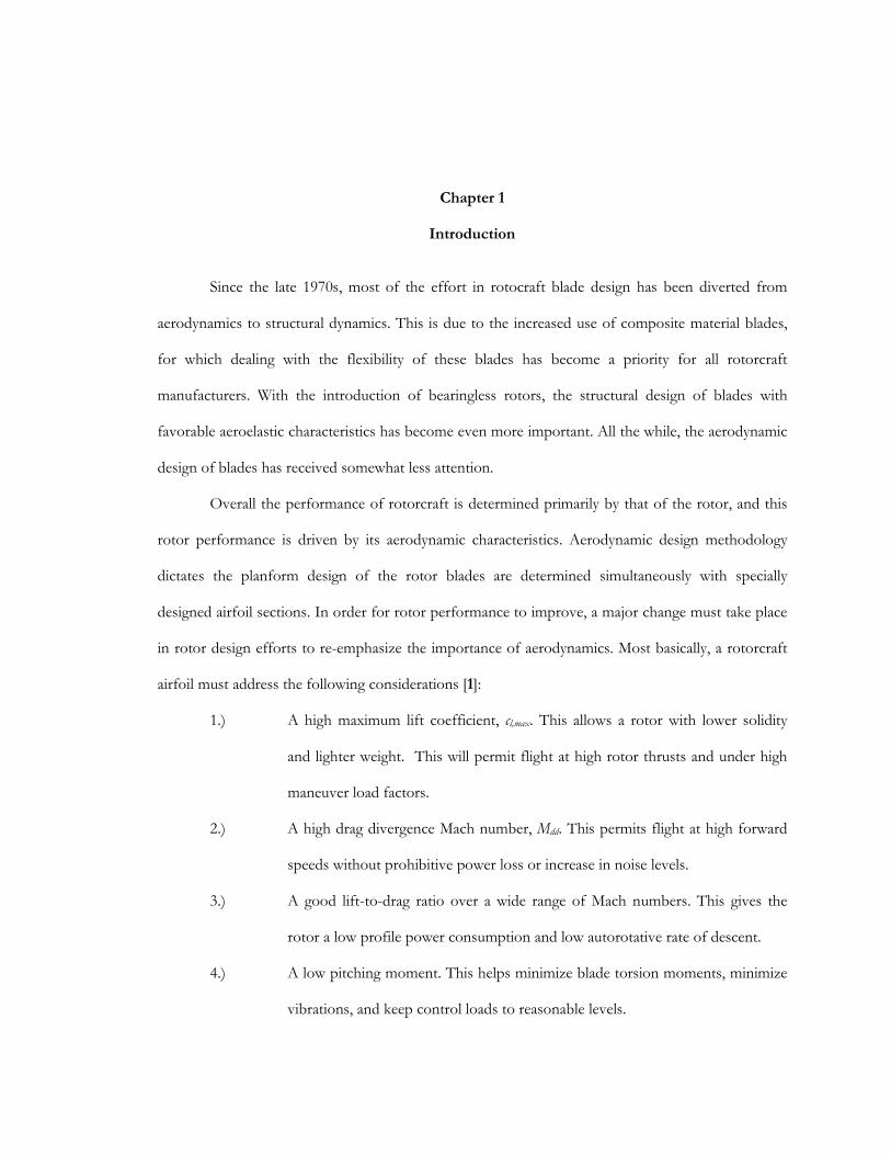
using cambered and thinner airfoils optimized along the length of the blade would meet the specific
local quasi-steady aerodynamic requirements as seen in Figure 1-3.
1.2.2 Modern Airfoils
Many modern airfoils stem from the classic NACA series. The second generation rotorcraft
airfoils showed significant changes from the baseline NACA airfoils. They were designed to meet the
requirements of the inboard and blade tips regions, and matched to the advancing and retreating
sides of the rotor disk.[9] The third and modern generation airfoils show modest improvements. It
seems that airfoil developments have essentially hit a plateau in terms of 2-D sectional performance.
This is because these airfoils are still designed for high lift, low drag, and low pitching moments at a
single Mach number, Reynolds number, and under steady flow conditions. Figure 1-4 shows the
geometric progression of airfoil design through the generations.
Figure 1-3: The weighted quasi-steady aerodynamic requirements for the blades are such that different airfoils must be employed at different radial stations.[8]

8
It is interesting to look at the historical trends of the blade loading coefficient, σTC , shown
in Figure 1-5. Also, the United States Army uses this metric as a way to measure the performance of
helicopters and set their Technology Development Approach (TDA).[10] The TDA goals are shown
on Figure 1-5, which show 16% and 24% improvements in σTC by 2005 and 2010, respectively.
The graph shows that the performance has not changed very much after 50 years of development. It
should be noted, the lower values for combat helicopters are attributed to the larger stall margin
needed for the maneuvering requirements.
Figure 1-4: A selection of rotorcraft airfoils through the generations.[8]

9
1.3 Flow Control
To increase the performance of the existing single element airfoils, the use of passive and
active flow control devices has been investigated by multiple agencies. Research has shown that
perhaps a 5-10% increase in the rotor’s figure of merit and an expansion of the flight envelope of the
helicopter.[8]
1.3.1 Boundary-Layer Control
One method of reducing profile drag that has been researched on various aircraft is
boundary layer control. Here, the growth of unstable disturbances in the laminar boundary layer that
induce a transistion to turbulent flow are suppressed. Over the past few decades, many concepts of
using suction and blowing (or combinations thereof) have been investigated to control the
development of the boundary layer on aerodynamic surfaces. This, however, has many challenges in
implementation on aircraft, not to mention helicopters due to the volume and structural restraints of
Figure 1-5: Historical trends in rotor blade loading.[8]

10
the rotor blades. Few of the concepts have been successful and even fewer have been used on
production aircraft.[11] No boundary layer control devices have been used on helicopters due to the
added weight, need of power and complexity of the required pumps and tubes to actuate the system.
There have been numerous problems also of the pores becoming clogged due to adverse
environmental conditions.
1.3.2 Zero-Mass Flow Synthetic Jets
The use of zero-mass synthetic jets (SJA) is concept of flow control that has been
investigated in recent years.[12] These devices have shown increases in airfoil cl,max and decreases in
profile drag. The synthetic jets are produced by a diaphragm inside the SJA that is vibrated to
energize the flow without adding any mass to the system. A schematic can be seen in Figure 1-6. The
interaction of the ejected flow with the external boundary layer energizes the flow and suppresses the
onset of separation. While the exact effects of SJAs on the flow are still unknown, initial
investigations have shown sizable increases in 2-D airfoil performance. SJAs also have an advantage
over traditional boundary layer control methods, as SJAs do not require a supply of compressed air
or the use of associated tubing, piping or values.
Figure 1-6: Schematic of a synthetic jet actuator (SJA).[8]

11
1.4 Miniature Trailing-Edge Effectors
Miniature Trailing-Edge Effectors, or MiTEs, are another flow control concept that have
been considered for use on lifting surfaces.[13] Aerodynamically, MiTEs, depicted in Figure 1-7, are
as effective as plain flaps, and high frequency deployments are achievable due to their small size.
Experments showed success with their use in flutter stabilization.[14] Seen in Figure 1-7, these
MiTEs remained effective at frequencies exceeding 125 Hz. Also, their use has been investigated for
rotor-blade control.[15,16] These studies positioned the MiTEs on the upper and lower surfaces of
the airfoil upstream from the trailing-edge. This provides aerodynamic control at the outboard
stations of the rotorblade, and reduces the high loading at the root of the blade.
1.4.1 Background
MiTEs are essentially an actively actuated Gurney flap. The Gurney flap was first used in
1971 by race car driver Dan Gurney as an experimental fix during the testing of a poorly performing
racecar. The device is beneficial for providing racecars with an efficient, alterable means to increase
the downward force on the wings.[17] This downward force is used to increase the traction of the
vehicle, thereby increasing cornering speeds.
Figure 1-7: Concept of MiTE[13]

12
To gain a better understanding of this new aerodynamic flap, Gurney brought the flap to the
attention of McDonnell Douglas aerodynamicist, Robert Liebeck. He investigated the aerodynamics
of the Gurney flap and introduced their application to the aircraft industry. In this investigation,
Liebeck hypothesized the flow structure around a Gurney flap as shown in Figure 1-8, where two
counter-rotating vortices form behind the flap and effectively increase the airfoil’s camber near the
trailing edge.[18]
Experiments were done to investigate the effects of Gurney flaps with respect to the
thickness of the boundary layer.[19] It was observed that Gurney flaps were effective when the
heights were at the same scale as the boundary layer. When the boundary layer was significantly
thicker than the flap, there was essentially no effect on the lift of the airfoil. The study postulated that
the attached counter-rotating vortices act as a means for the airfoil to attain an "off-the-surface
pressure recovery," allowing for a large discontinuity in the surface pressure at the trailing edge. This
effectively shifts the Kutta condition downstream and below the physical trailing edge.
In other experiments, laser Doppler anemometry (LDA) was used to obtain detailed flow
structures near Gurney flaps.[20-22] These results displayed the von Kármán vortex street that forms
downstream of the Gurney flap and when time averaged, resulted in Liebeck's hypothesized flow
Figure 1-8: Liebeck’s hypothesized flow structure around MiTE.[18]

13
structure. Also, the frequency of these oscillations was observed to depend on the height of the
Gurney flap and boundary layer thickness.
There has been some interest in using MiTEs for vibration control on rotorcraft. The major
concern is their ability to achieve increments in the lift and pitching moment at high frequencies. As
Gurney flaps are effective on both the upper and lower surfaces, MiTEs can achieve twice the
amplitude of the lift and pitching moments if used on both surfaces. After the flow separates
however, they become increasingly submerged into the boundary layer and have thus has no affect
on the aerodynamic loads. This behavior is also true for MiTEs. Also, Gurney flaps have been shown
to be effective if placed upstream of the trailing edge but the performance gains are not as great.[15]
Table 1-1 shows the effects of a 1 percent chord lower-surface Gurney flap on a variety of
airfoils. The max,lc∆ over the baseline airfoil remains fairly consistent amongst all the airfoils
displayed. Figure 1-9 plots max,lc∆ versus max,lc of the baseline airfoil. It is seen that the effects of the
Gurney flap decreases as the baseline max,lc increases. The effects of a static Gurney flap can be
roughly approximated by this trend.
Table 1-1: Summary of 1 percent chord height Gurney flap effect to max,lc .[19,23-25,35]

14
In rotorcraft applications, Gurney flaps have been used on the horizontal tail to increase its
authority for high-powered climbs. They have also been investigated for the improvement of rotor
performance for both helicopters and wind turbines. One study used a model helicopter with Gurney
flaps showed increases in the rotor performance at high thrusts and in forward flight. However, it
was also observed that at lower thrusts and hover, the Gurney flaps decrease the performance. It is
because of this decrease in performance that passive Gurney flaps are not practical for overall
performance gains.[27]
1.4.2 Rotor Applications
MiTEs have many potential applications on rotorcraft. The ability to actuate Gurney flaps
makes them a very capable aerodynamic device on rotorcraft.
Figure 1-9: Summary of 1 percent chord height Gurney flap effects to the maximum lift for several airfoils at varying flow conditions.[26]

15
1.4.2.1 Individual Blade Control
For helicopters, vibration reduction is a major area of research in effort to improve the ride
qualities over that of current vibration control systems. Methods of higher harmonic control (HHC)
and Individual Blade Control (IBC) have been investigated for these applications. The idea behind
these concepts is to create aerodynamics loads at frequencies corresponding to those that are felt in
the fuselage and therefore cancel the vibrations. The requirement for these loads is on the order of
4/rev or about 20 Hz. In particular for IBC, active flaps have been considered in numerous studies.
MiTEs could be used in place of these active flaps as they appear to be ideal in providing the
required changes in lift and moments required. An additional advantage of using MiTEs are that they
provide this potential with significantly lower actuator loads and are insensitive to compressibility
effects.[23,28]
1.4.2.2 Rotor Performance Enhancement
A major study was conducted recently by Michael Kinzel to investigate the use of MiTEs on
rotorcraft. The goals of the project were to first model the aerodynamic characteristics of MiTEs,
and then investigate the potential rotor performance improvements.[26] This includes increasing the
maximum flight speed, achievable rotor thrusts, thrusting performance, maneuver performance and
payload capabilities. These gains would indirectly increase the cruise performance. MiTEs show to be
most effective for transonic airfoils, as they provide a more efficient configuration for high-speed
flows, while still providing high lift when needed. These increases in the maximum lift indirectly
improve the cruise performance of the helicopter, by allowing the blade to be designed for transonic
flow, without losses in the maximum flight speed and high thrust performance. Deployment
schedules of MiTEs were also studied, showing that MiTEs are equally effective using on/off
actuation or gradual deployment. Finally, the performance gains that MiTEs provide at high speeds

16
and for high thrusts depend more on the capability to increase the lift and prevent stall. Figure 1-10
shows the increase in the maximum forward speed of a MiTE-equipped helicopter.
MiTEs provide lift and pitching moment increments that are comparable to those of plain
flaps. One advantage of a MiTE in this application is that the actuation loads required are much less.
The decreased actuation loads are due to the hinge moment being essentially zero compared to those
of a trailing-edge flap. A MiTE’s low inertia also allows for high frequency response.
All of the performance analysis done in this initial research was done on MiTEs placed at the
trailing-edge of the airfoil. The study that continues in the following chapters extends this research to
MiTEs placed upstream of the trailing-edge. Previous experiments showed a decreased in the
Figure 1-10: Comparison between baseline and MiTE rotor performance in level forward flight with variations in the gross weight calculated using the dynamic stall model and without an optimal MiTE deployment schedule.[26]
17
effectiveness of an upstream MiTE; however, this placement is advantageous in that it allows the
retracted MiTE to be buried within the airfoil.
1.4.2.3 Other Potential Applications of MiTEs
There are a wide range of other applications of MiTEs to rotorcraft. These devices can be
used for any function where IBC systems can provide benefits. IBC systems are often suggested for
their usage to alter the rotor wake for noise control, for which purpose a MiTE could deploy to
affect the tip vortices and their interactions with other rotor blades. The vortex miss distance from
the blade can be increased and, therefore, the noise generated by blade-vortex interactions reduced.
In another application, the vortices can influence and reduce the angle of attack on the retreating
blades to delay stall.

Chapter 2
Experimental and CFD Investigations
In order for an aerodynamic model to be formulated, a number of experimental studies were
utilized for understanding and validation. Likewise, due to the complex nature of a MiTE on a
rotorcraft, a single wind tunnel experiment was not feasible. Therefore, multiple experiments were
investigated and used in validating a Computational Fluid Dynamics (CFD) simulation that was then
used as a “virtual” wind tunnel.
2.1 Static Wind Tunnel Testing
The first experiment was that of an airfoil tested in a wind tunnel with and without Gurney
flaps attached at and near the trailing edge.[35] Surface pressure measurements were used to
determine the lift and pitching moment of the airfoil, while a wake-traverse probe was used to obtain
the drag. The airfoil was initially tested in its baseline state then with Gurney flaps of 0.005c, 0.01c
and 0.02c in height located at 0.9c, 0.95c and 1.0c. All of these configurations were tested with
natural and fixed transition, a chord Reynolds number of 1.0x10⁶, and a Mach number of less than
0.2. While previous tests of Gurney flaps used a force balance, this particular experiment’s surface
pressure integration showed how the flaps affected the pressure distributions to achieve higher lift
coefficients.
2.1.1 Wind Tunnel Description and Airfoil Model
The wind tunnel used for the static airfoil testing was the Penn State Low-Speed, Low-
Turbulence Wind Tunnel. This facility is a closed throat, single-return atmospheric wind tunnel that

19
has a maximum test section velocity of approximately 220 ft/s. The test section is rectangular
measuring 3.25 ft high and 4.75 ft wide with filleted corners, as seen in Figure 2-1.[29]
The surface pressure measurements on the model are reduced to pressure coefficients and then used
to determine the sectional force and moment (about the quarter-chord) coefficients. The sectional
profile drag coefficients are obtained through use of the wake traversing probe and total pressures
using momentum theory.[30,31]
The airfoil model used was the 12-percent thick S903 airfoil.[32] This airfoil was designed to
explore the effects of airfoil thickness and surface roughness on the maximum lift coefficient of wind
turbines. While this airfoil was designed for large amounts of laminar flow, it is similar to many
rotorcraft airfoils in terms of thickness ratio and camber distribution. Figure 2-2 compares the S903
airfoil with the Boeing-Vertol VR-12, a well-known rotorcraft airfoil.[33]
Figure 2-1: The 3.25' x 4.75' cross section of the S903 airfoil placed in the Penn State Low-Turbulence, Low-Speed Wind Tunnel.

20
2.1.2 Experimental Results
Figures 2-3 and 2-4 show the pressure distributions for the baseline airfoil, the airfoil with a
0.02c high lower-surface Gurney flap at 1.0c and at 0.9c. At a constant lift coefficient of 0.7, the three
configurations are compared in Figure 2-3, while in Figure 2-4, they are compared at their maximum
lift coefficients of 1.15, 1.35 and 1.5 respectively.
Figure 2-2: The S903 airfoil compared to the VR-12 airfoil
Figure 2-3: Pressure distributions at cl = 0.7 with and without Gurney flaps

21
From Figure 2-3, it is shown that the Gurney flap greatly increases the pressure on the lower
surface of the airfoil upstream of the flap. On the upper surface of the airfoil, by alleviating the
pressures on the trailing edge with the Gurney flaps, the leading-edge suction peak is reduced and the
start of pressure recovery is moved aft by approximately 20 percent chord. Along with the delay, the
pressure at which recovery begins is much lower than that of the original airfoil. This relaxing of the
pressure recovery allows the airfoil to have more favorable gradients over the forward part of the
airfoil.
As seen in Figure 2-4, large gains are made in terms of maximum lift coefficient between
that of the baseline airfoil and those of the flapped model. This is due to the large increases in lower-
surface pressure. At higher angles of attack, the Gurney flap becomes more effective due to the
thinning of the lower-surface boundary layer. The lowering of pressure levels in the pressure
recovery on the upper surface also aided in greater maximum lift coefficients attained and moved the
point of separation downstream by 15 percent chord. The cause of differing lift coefficients between
Figure 2-4: Pressure distributions at cl.max with and without Gurney flaps

22
the two Gurney flap locations is mostly due to the earlier pressure gain on the lower surface for the
upstream Gurney flap. This results in a loss of lift production from the location of the flap to the
trailing edge.
Figure 2-5 shows the influence of Gurney flap height on the aerodynamic characteristics of
the airfoil. A 0.02c Gurney flap placed at the trailing edge achieves a 29 percent increase in maximum
lift coefficient compared to the baseline airfoil. The shorter flaps also show gains in maximum lift
coefficient and were proportional to their size. As the boundary layer thins on the lower surface with
increasing angles of attack, the Gurney flap on that surface becomes more effective and causes the
lift-curve slope to increase. Conversely, as the angle of attack decreases, the effect of the Gurney flap
decreases. This results in the lift curves merging with that of the baseline airfoil as the negative
maximum lift value is approached. The moment curves behaved in a similar manner with increasingly
negative angles of attack. At angles of attack for which the Gurney flaps are effective, the increased
aft loading due to the flap results in increasing nose-down pitching moment coefficients compared
with the baseline airfoil. The change in the pitching moment is also proportional to the Gurney flap
height. Although the magnitude of pitching moment coefficients might be of concern, the actually
moments remain small for MiTEs deployed on the retreating blade side due to low dynamic pressure.
Within the low-drag region just as with the lift and pitching moments, the minimum drag rises
approximately proportional to the Gurney-flap height.

23
Due to the physical constraints of MiTE deployments normal to the surface, the flap must
be placed far enough upstream to be completely buried within the airfoil when not deployed.
Figure 2-6 shows the aerodynamic gains achieved with Gurney flaps are only moderately reduced by
upstream MiTEs. The maximum achievable lift coefficient is reduced by approximately 10 percent as
a 0.02c flap is moved to 0.90c from the trailing-edge location. Similar changes are seen with the
pitching moment coefficient. The changes in drag, however, seem to only change with the Gurney
flap height and not with its location.
Figure 2-5: Aerodynamic characteristics with varying Gurney flap heights, at the trailing edge

24
Although the S903 is similar to the VR-12 rotorcraft airfoil, the S903 was designed to make
use of natural laminar flow to achieve low drag. To explore how the airfoil aerodynamics would be
altered on an airfoil such as the VR-12, measurements were also made with transition fixed at 0.02c
on the upper surface and 0.05c on the lower surface of the airfoil. The primary interest is the
aerodynamic behavior near the maximum lift coefficient, the turbulator grit was sized to the critical
roughness height for angles of attack approaching stall.[34] Thus, at lower angles of attack, the grit is
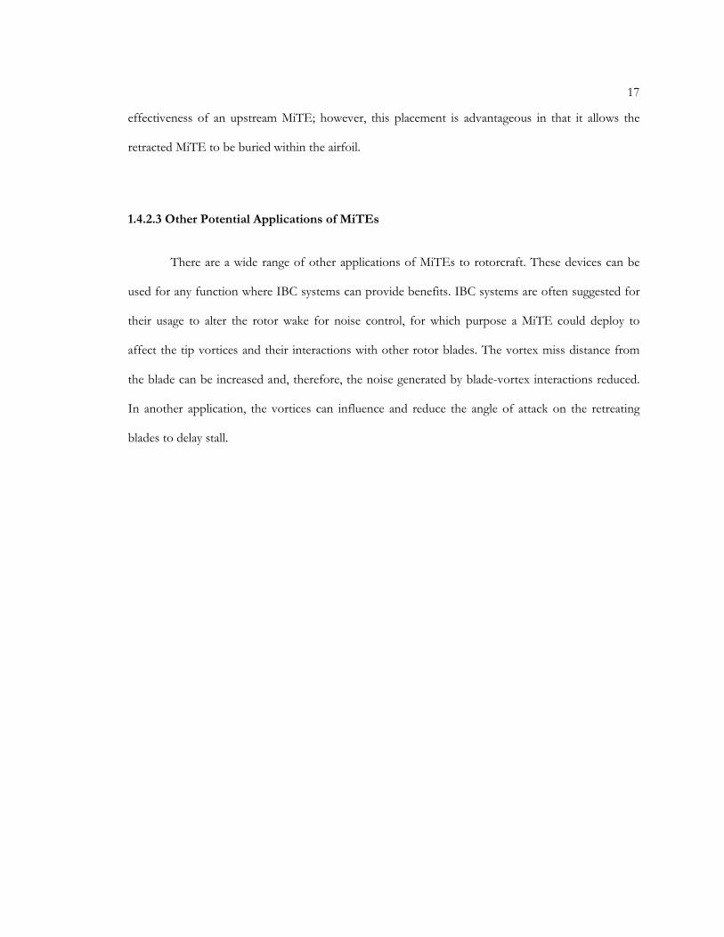
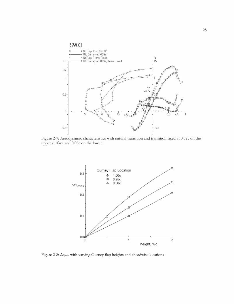
too small to force transition. Figure 2-7 shows this by the converging drag curves of the free and
forced transition configurations at lower angles of attack. Also, it is seen that the while the drag
increases with fixed transition, the lift and moment curves are essentially unaffected. With fixed
transition, the drag increases due to the Gurney flap is not nearly as large as it is with free transition,
especially in the case of the baseline airfoil that has significant amounts of laminar flow. Again, the
fixed transition results are more representative of an operational rotorcraft environment. The effect
of Gurney flaps in terms of height and location are summarized in Figure 2-8.
Figure 2-6: Aerodynamic characteristics with varying Gurney flap chord-wise locations
25
Figure 2-7: Aerodynamic characteristics with natural transition and transition fixed at 0.02c on the upper surface and 0.05c on the lower
Figure 2-8: ∆cl,max with varying Gurney flap heights and chordwise locations
26
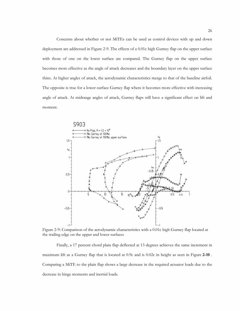
Concerns about whether or not MiTEs can be used as control devices with up and down
deployment are addressed in Figure 2-9. The effects of a 0.01c high Gurney flap on the upper surface
with those of one on the lower surface are compared. The Gurney flap on the upper surface
becomes more effective as the angle of attack decreases and the boundary layer on the upper surface
thins. At higher angles of attack, the aerodynamic characteristics merge to that of the baseline airfoil.
The opposite is true for a lower-surface Gurney flap where it becomes more effective with increasing
angle of attack. At midrange angles of attack, Gurney flaps still have a significant effect on lift and
moment.
Finally, a 17 percent chord plain flap deflected at 13 degrees achieves the same increment in
maximum lift as a Gurney flap that is located at 0.9c and is 0.02c in height as seen in Figure 2-10 .
Comparing a MiTE to the plain flap shows a large decrease in the required actuator loads due to the
decrease in hinge moments and inertial loads.
Figure 2-9: Comparison of the aerodynamic characteristics with a 0.01c high Gurney flap located at the trailing edge on the upper and lower surfaces

27
2.2 NASA Ames Dynamic Wind Tunnel Testing
Experiments investigating an oscillating airfoil with a Gurney flap were conducted at the
NASA Ames Research Center in the Compressible Dynamic Stall Facility (CDSF) using the VR-12
rotorcraft airfoil.[36-38] The point of these tests was to increase the understanding of Gurney flaps
in compressible dynamic stall. The test matrix consisted of an airfoil with a Gurney flap located at the
trailing edge oscillated at reduced frequencies, k, of 0.0, 0.05 and 0.1 where the reduced frequency is
defined as
Figure 2-10: Comparison of plain flap and MiTE
V
ck
2
ω= 2.1

28
The airfoil rotates about the quarter chord such that )sin(1010)( tt ωα °+°= . The Reynolds
number ranged from 0.7x10⁶ to 1.6x10⁶ with Mach numbers of 0.2, 0.3 and 0.4. The Gurney flap
heights investigated were 0.0085c, 0.0135c and 0.024c.
The lift, pressure drag and pitching moment calculations were done through the use of
surface pressure integrations. The surface pressure measurements were done using 20 Kulite
unsteady-pressure transducers that measured the absolute pressure. Typically the sampling rate was 4
kHz/channel, and totally 40,000 samples/channel were recorded and stored according to bins based
on the angle of attack, with increments ranging from 0.02 to 0.08 degrees. The data was stored in 800
bins and then averaged. A minimal standard deviation was observed giving confidence that
uncertainty is low. Using the geometry and instantaneous angle of attack, the lift, pressure drag and
pitching moment coefficients was calculated. The viscous drag is neglected, as this quantity is
relatively small at angles of attack corresponding to dynamic stall. The pressures on the faces of the
Gurney flap were not measured.
2.2.1 Wind Tunnel Description and Airfoil Model
The CDSF, shown in Figure 2-11, is an in-draft wind tunnel with a test section measuring 35
cm high, 25 cm wide and 100 cm long and designed to operate at Mach numbers up to 0.5.[37] The
mounting system has the capability to continuously vary the airfoil pitch angle at amplitudes varying
from 2 to 10 degrees, and using mean airfoil pitch angles of 5, 10 or 15 degrees. The mean pitch
angle can also be set to other angles by manually adjusting the angle of attack assembly.[37,38]

29
The chord length of the model is 15.2 cm and its span is 25 cm.[38] Baseline cases that have
zero droop are of interest for this study. These results are used in the validation the CFD modeling
of MiTEs. Fabrication requires that the trailing edge be constructed as shown in Figure 2-12, and the
leading edge surface of the model is relatively rough. Comparisons of static polars of the VR-12
airfoil as designed and that of the fabricated model for this experiment are shown in Figure 2-13.
These polars are generated using MSES,[39] at conditions similar to those of the wind tunnel, with
the transitions fixed near the leading edge.
Figure 2-11: Compressible Dynamic Stall Facility at NASA Ames

30
Figure 2-14 shows the predicted pressure distributions of the designed and fabricated
airfoils agrees well at an angle of attack of 10 degrees. This gives confidence that the fabricated
model will predict the correct characteristics of the VR-12 airfoil in dynamic stall. Minor
Figure 2-12: Comparison of the trailing edge profiles of the designed VR-12 airfoil to that fabricated for experiments
Figure 2-13: Comparison of the static polars of the designed VR-12 airfoil to that fabricated for experiments, as calculated by MSES at M=0.4, Re =1.4e6

31
discrepancies will occur because of the fabricated model having an increased stall angle of attack, and
a lower max,lc than the designed VR-12 airfoil.
2.2.2 Experimental Results
Quasi-steady results at M=0.3 are shown in Figure 2-15 for the airfoil in the positive-pitch
stroke. These results are useful since they display the static effects of the Gurney flap post stall. This
is of importance for rotor modeling purposes where these post-stall Gurney flap effects are used for
dynamic stall modeling. Recall that the experiments do not measure the Gurney flap pressures or the
viscous drag; thus, as observed in Figure 2-15, for lower angles of attack the Gurney flap shows a
decrease in the pressure drag. If these additional quantities are measured, the airfoil using a Gurney
flap would in fact increase the drag as observed in the static-airfoil wind-tunnel experiments. Finally
notice that the Gurney flap continues to be effective post stall.
Figure 2-14: Comparison of the pressure distribution the designed VR-12 airfoil to that fabricated for experiments

32
The results from the oscillating airfoil experiments are presented in Figures 2-15 to 2-18 for
a 0.0135c height Gurney flap at Mach numbers of 0.3 and 0.4 and a reduced frequency of 0.05. In
Figure 2-16, the lift coefficient is plotted against the angle of attack. It can be observed that in
dynamic stall, this Gurney flap increases maximum lift by 22 percent. Gurney flaps also have the
effect of decreasing the stall angle of attack with an increase in flap height.[38] This decreased stall
angle of attack is expected, as a similar behavior occur statically.
(a) (b) Figure 2-15: The quasi-steady experimental results comparing the VR-12 baseline and with a 0.0135c height Gurney flap through stall at M=0.3. (a) lift and drag (b) Gurney flap effects of lift and drag

33
The drag is compared in Figure 2-17, where nearly constant increases are observed at angles
less than stall. Post stall, the Gurney flap results in a much larger increase in drag. This is due to the
increased vortex effects and because the airfoil is in a deeper stall when compared to the baseline
airfoil.
(a) M=0.3 (b) M=0.4 Figure 2-16: Comparison of the lift for the VR-12 baseline airfoil and with a 0.0135c height Gurney flap in dynamic stall at a reduced frequency of 0.05
(a) M=0.3 (b) M=0.4
Figure 2-17: Comparison of the drag for the VR-12 baseline airfoil and with a 0.0135c height Gurney flap in dynamic stall at a reduced frequency of 0.05

34
A better comparison is made in the plot of cl versus cd in Figure 2-18 as it shows the increase
in aerodynamic efficiency at high lifts. These results are consistent with the static results, and if the
profile drag were measured, would show that the aerodynamic efficiency is increased at high lifts
using Gurney flaps.
The pitching-moment coefficient is compared in Figure 2-19. It can be seen that there is
nearly an offset in an increased nose-down pitching moment. With delaying stall to higher lifts results
in the nose-down pitching moments being decreased at high lifts.
(a) M=0.3 (b) M=0.4
Figure 2-18: Comparison of the drag polars for the VR-12 baseline airfoil and with a 0.0135c height Gurney flap in dynamic stall at a reduced frequency of 0.05

35
2.3 Wind Tunnel Experimental Conclusions
From these two experiments, the understanding of Gurney flaps behavior has been
improved. These results suggest that Gurney flaps can provide similar lift increases upstream of the
trailing edge, when compared to the traditional placement at the trailing edge of an airfoil. There is a
performance penalty associated with this upstream placement, but such a concept is essential for the
implementation of actuating MiTEs. Lift and moment changes are achievable in either the positive or
negative directions, depending on the surface which the Gurney flap is placed.
In considering the effects of a Gurney flaps to oscillating airfoils, the results resemble those
found statically. Furthermore, the increase in cl,max and the change in αstall for an oscillating airfoil are
similar to static airfoils. Finally, at higher lifts, the Gurney flap is observed to increase the
aerodynamic efficiency, while simultaneously lower pitching moment by delaying the effects of
dynamic stall to increased lifts.
(a) M=0.3 (b) M=0.4 Figure 2-19: Comparison of the pitching moment for the VR-12 baseline airfoil and with a 0.0135c height Gurney flap in dynamic stall at a reduced frequency of 0.05

36
2.4 CFD Investigations
Ideally, more experimental testing would be done to investigate the application of MiTEs.
These experiments, however, are not practical for initial investigations due to their cost and
complexity where the test would involve an oscillating airfoil, at various flow conditions and having
flaps that deploy at high frequencies. This being the situation, computational methods are the best
tool for this initial stage of research. CFD calculations are most valuable in investigating complex
problems such as these where one can gain a better understanding of the physical flow characteristics
present.
The NASA CFD code, OVERFLOW2, was validated and used for the analysis of Gurney
flaps and MiTEs.[26] OVERFLOW2 is a Reynolds averaged Navier-Stokes (RANS) solver that
utilizes structed Chimera overset grids that allow for relative motion between bodies.[40,41] These
simulations use the Spalart-Allmaras one-equation turbulence model, which is specified for all
boundary layers which are modeled as fully turbulent.[42] An inherent consequence of this method is
that the laminar regions are also modeled at turbulent. This simplification is because OVERFLOW2
does not incorporate a transition model. While this is not completely modeling the true
characteristics of the flow, helicopter airfoils are typically designed using a fully turbulent model and
thus the simplification is an acceptable approximation.[8]
2.4.1 Gurney Flapped Airfoils
Due to the environment of the helicopter rotor, the performance of MiTEs at a range of
Mach numbers needs to be investigated. Transonic experiments and CFD research have shown that
the effects of Gurney flaps are similar in transonic flows, as observed in low-speed experiments.
Unfortunately, data does not exist for Gurney flaps at varied Mach numbers on a consistent airfoil.
This data is needed to successfully model the effects of Gurney flaps and MiTEs in order to apply

37
them to rotorcraft. To do this, CFD was used to analyze the Gurney flaps at several Mach Numbers.
The airfoils used were the Boeing-Vertol high-lift VR-12 and transonic VR-15 airfoils which are two
heavily used rotorcraft airfoils.
2.4.1.1 VR-12: 0.01c Gurney Flap located at 1.0c
The VR-12 airfoil is representative of inboard regions on the rotor. The Gurney flap effects
at various Mach numbers for the VR-12 are seen in Figure 2-20.
(a) (b)
(c)
Figure 2-20: Gurney flap effects with Mach number variations for the VR-12 airfoil (a)lift increment (b) drag increment (c) moment increment
38
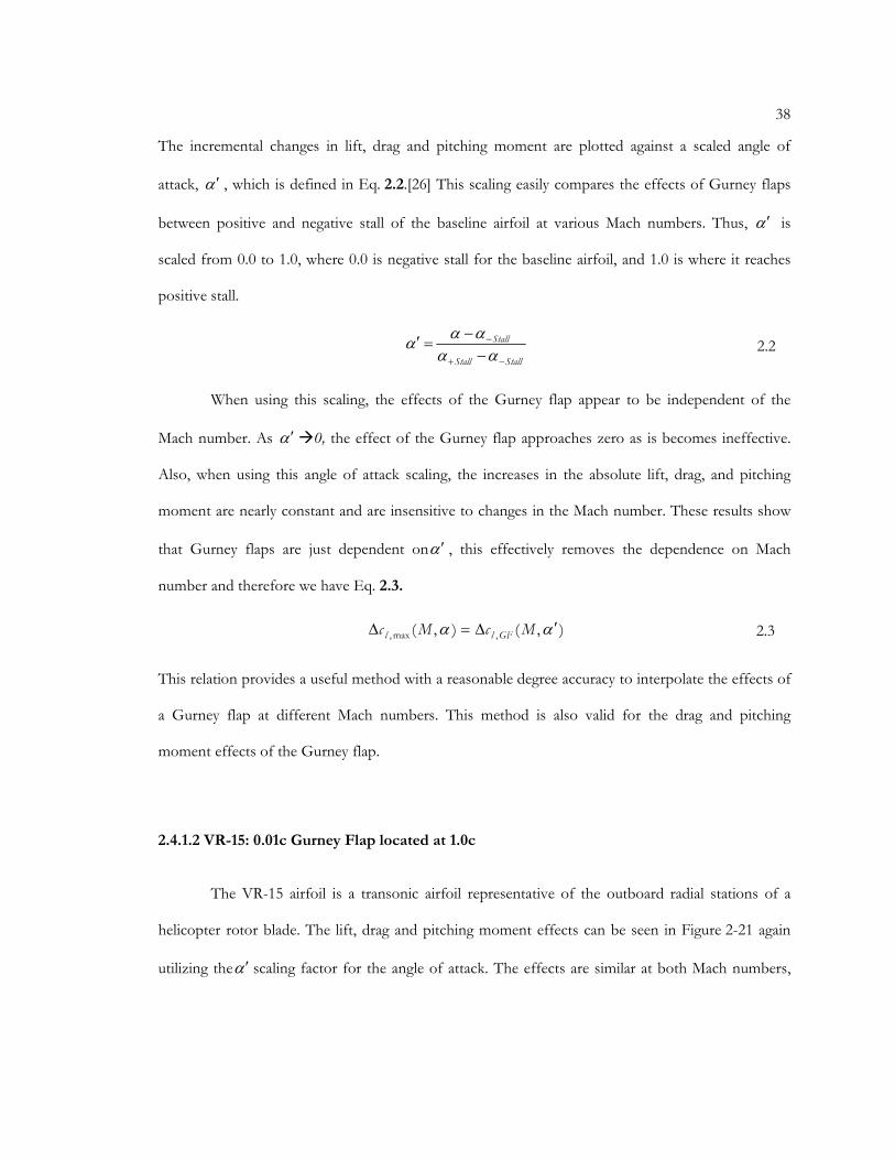
The incremental changes in lift, drag and pitching moment are plotted against a scaled angle of
attack, α ′ , which is defined in Eq. 2.2.[26] This scaling easily compares the effects of Gurney flaps
between positive and negative stall of the baseline airfoil at various Mach numbers. Thus, α ′ is
scaled from 0.0 to 1.0, where 0.0 is negative stall for the baseline airfoil, and 1.0 is where it reaches
positive stall.
When using this scaling, the effects of the Gurney flap appear to be independent of the
Mach number. As α ′�0, the effect of the Gurney flap approaches zero as is becomes ineffective.
Also, when using this angle of attack scaling, the increases in the absolute lift, drag, and pitching
moment are nearly constant and are insensitive to changes in the Mach number. These results show
that Gurney flaps are just dependent onα ′ , this effectively removes the dependence on Mach
number and therefore we have Eq. 2.3.
This relation provides a useful method with a reasonable degree accuracy to interpolate the effects of
a Gurney flap at different Mach numbers. This method is also valid for the drag and pitching
moment effects of the Gurney flap.
2.4.1.2 VR-15: 0.01c Gurney Flap located at 1.0c
The VR-15 airfoil is a transonic airfoil representative of the outboard radial stations of a
helicopter rotor blade. The lift, drag and pitching moment effects can be seen in Figure 2-21 again
utilizing theα ′ scaling factor for the angle of attack. The effects are similar at both Mach numbers,
StallStall
Stall
−+
−
−−
=′αα
ααα 2.2
),(),( ,max, αα ′∆=∆ McMc GFll 2.3

39
however, not at good at the VR-12 results. This is a result of using a small number of discrete angles
of attack and would cause Stall+α and Stall−α not to be fully resolved.
(a) (b)
(c)
2.4.2 Dynamic MiTE CFD Results
MiTEs are intended to perform two functions in their application to rotorcraft. The first is
that of fuselage vibration control which requires deployment to occur at or near 4/rev (20Hz). The
Figure 2-21: Gurney flap effects with Mach number variations for the VR-15 airfoil (a)lift increment (b) drag increment (c) moment increment
40
second application is to increase rotor performance which requires 1/rev deployments (5Hz). At this
frequency, the MiTEs increase the sectional cl,max to delay the onset of dynamic stall. CFD
calculations were conducted at both frequencies to study the aerodynamics at a constant angle of
attack.
2.4.2.1 VR-12 Airfoil: 0.01c height MiTE at 1.0c
The first case was that of a VR-12 airfoil with a MiTE height of 0.01c at the trailing edge
where deployments were done at numerous frequencies and flow conditions. The results can be seen
in Figure 2-22 through Figure 2-24. The normalized lift is compared to Theodorsen’s theory in
Figure 2-23(a).[43] The CFD shows excellent agreement in both amplitude and phase-lag trends.
One difference is that the normalized lift magnitude for the MiTE approaches 0.4 as ∞→k , while
Theodorsen’s function approaches 0.5. There is also a difference at high Mach numbers between the
CFD results and Theodorsen’s theory which is due to the incompressible assumptions made in it.
The CFD results also show that when the Mach number is increasing, as 0→k , the lift magnitude
and phase lags are increased which follows compressible-unsteady theory. The phase difference at
low Mach numbers is due to the Theodorsen function only accounting for circulatory loads where
the apparent mass effects would be a factor at this particular flow condition. These apparent mass
loads have a 90 degree phase lead that becomes more evident for high frequency flapping. The CFD
data also correlates very well with the lift data of a NACA 0012 at a Mach number of 0.1 seen in
Figure 2-23.[14]

41
(a) (b)
Figure 2-22: Force and moment for the sinusoidal deployment of a 0.01c MiTE located 1.0c, compared to static wind-tunnel data. (a) ω=5Hz (k=0.14) (b) ω=20Hz (k=0.54)

42
Figure 2-23: Effect of the lift with changes in deployment frequency for a MiTE located at 1.0c, at various free-stream conditions, and compared to incompressible theories
Figure 2-24: Effect of the drag and pitching moment with changes in deployment frequency of a MiTE located at 1.0c for various free-stream conditions

43
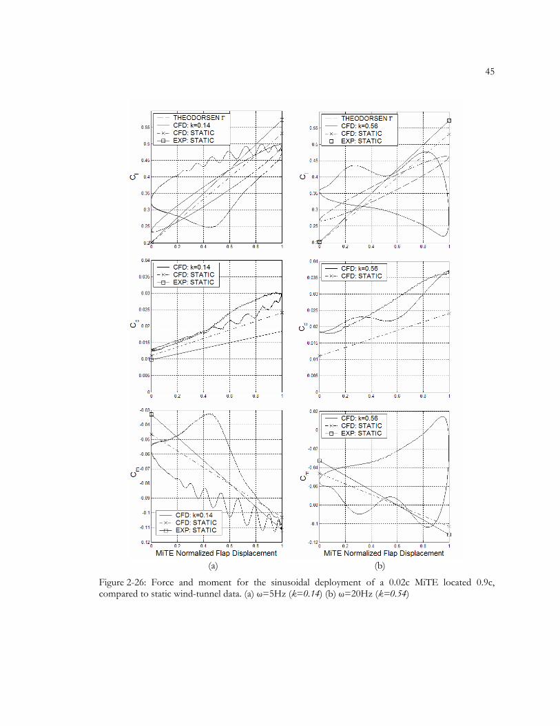
2.4.2.2 VR-12 Airfoil: 0.02c height MiTE at 0.9c
The case of a VR-12 model using a MiTE height of 0.02c positioned at 0.9c is investigated at
numerous frequencies and flow conditions. The results can be seen in Figure 2-26 through Figure 2-
28.
Figure 2-25 shows the instantaneous streamlines for the airfoil with a MiTE deploying at
5Hz.
At this lower deployment frequency, notice that in the retracted position, the flow near the MiTE is
stable. This is not the case when the deployment frequency is increased where visualizations show
that the flow is unattached downstream of flap. This is a result of subsequent deployments that occur
before the flow has time to reattach. As flap deploys, a strong vortex forms downstream of the MiTE
and convects to the trailing edge of the airfoil. The time required for this vortex convection is a
significant portion of the deployment cycle, especially for the 20Hz case.
This vortex has tremendous effects to the aerodynamics as shown in Figure 2-26, where the
two deployment frequencies are plotted and the lift can be compared to Theodorsen's function.
Observing the lift plots, notice that there are major deviations between the CFD results and theory.
Figure 2-25: Instantaneous streamlines calculated in OVERFLOW2 for a 0.02c height MiTE positioned at 0.9c, deploying at w=5Hz (k=0.14)

44
This does not discredit the CFD results, as the unsteady flow characteristics for this case clearly
violate assumptions made in Theodorsen's function. These assumptions are that the conditions are
an inviscid, incompressible, attached flow with only small disturbances. The flow around these
MiTEs show a large, unattached vortex that develops downstream of the MiTE, which suggests that
the solutions cannot be validated against analyses developed for conventional flaps and wings.
With further investigations of Figure 2-26, upon comparison of the lift amplitudes of CFD
and theory, the predicted amplitudes are comparable to the theory at both frequencies. There are
small positive offsets in the lift, suggesting that the MiTEs are shedding additional vortices into the
wake that induce upward velocities on the airfoil, and effectively increase the angle of attack. It is also
noticed that the MiTE does not achieve the maximum lift until the vortex reaches the trailing edge of
the airfoil. This is a result of the strong vortex that develops as the MiTE deploys, creating a low-
pressure region on the lower surface of the airfoil and counter produces lift. This is similar, but in the
opposing direction, to the vortex lift observed in dynamic stall.[1] Furthermore, flow visualizations
show that when the vortex reaches the trailing edge, the low-pressure core entrains air from the
suction surface and creates additional circulation over the entire airfoil. This entrained air also
balances the pressure and reduces the vortex strength, enabling the maximum lift to finally be
achieved. These combined effects attribute for these sharp increases in lift. The drag is noticed to
slightly increase for the low frequency case, where the flow has the time to reattach. For the high-
frequency case, where the time required for the vortex to reach the trailing edge approaches that of
the deployment cycle, the flow does not have time to reattach and the drag is significantly increased.
45
(a) (b)
Figure 2-26: Force and moment for the sinusoidal deployment of a 0.02c MiTE located 0.9c, compared to static wind-tunnel data. (a) ω=5Hz (k=0.14) (b) ω=20Hz (k=0.54)

46
Shown in Figure 2-27 is the normalized lift and phase angles compared to Theodorsen’s
function. Here the phase lags between the full deployment position and the maximum lift, and
between the fully retracted position and the minimum lift, are plotted separately as they vary
significantly. The lift amplitudes predicted by the CFD are larger than those of predicted by theory
and the phase lags also differ from those predicted by theory. Also, with increasing deployment
frequency, the phase lag increases which differs from what is predicted from theory. As a final note
in terms of the lift of the system, the phase lag at the minimum lift position is much larger than that
at the maximum lift. This is a result of a vortex system that develops behind the MiTE on the lower
surface of the airfoil.
Figures 2-28 and 2-29 summarize the drag and moment calculations in the reduced
frequency domain, with variations of the free-stream conditions. Notice that one case is simulated at
an angle of attack of 10 degrees, which unintentionally, falls in between the stall angles of attack of
the baseline airfoil and one with a Gurney flap. This is representative of a type of dynamic stall
occurring to a static airfoil, and would account for the large increases in the drag. The pitching
Figure 2-27: Effect of the lift with changes in deployment frequency of a MiTE located at 0.9c for various free-stream conditions compared to incompressible theories
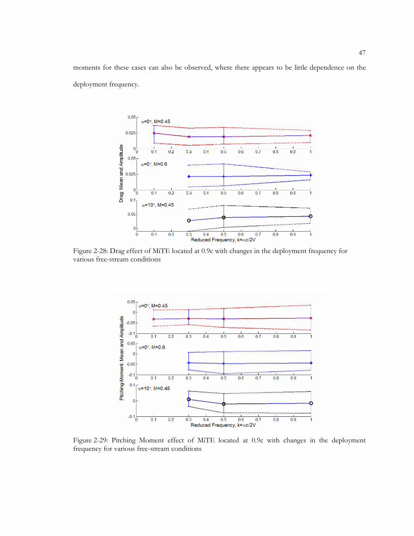
47
moments for these cases can also be observed, where there appears to be little dependence on the
deployment frequency.
Figure 2-28: Drag effect of MiTE located at 0.9c with changes in the deployment frequency for various free-stream conditions
Figure 2-29: Pitching Moment effect of MiTE located at 0.9c with changes in the deployment frequency for various free-stream conditions
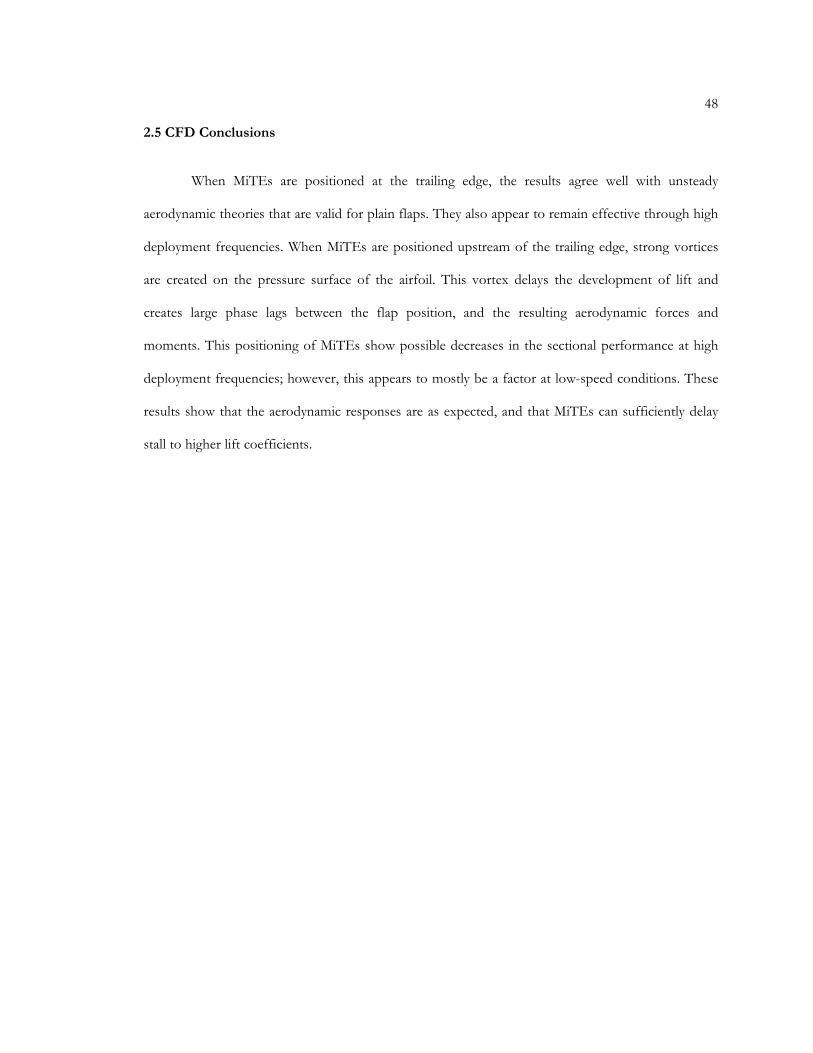
48
2.5 CFD Conclusions
When MiTEs are positioned at the trailing edge, the results agree well with unsteady
aerodynamic theories that are valid for plain flaps. They also appear to remain effective through high
deployment frequencies. When MiTEs are positioned upstream of the trailing edge, strong vortices
are created on the pressure surface of the airfoil. This vortex delays the development of lift and
creates large phase lags between the flap position, and the resulting aerodynamic forces and
moments. This positioning of MiTEs show possible decreases in the sectional performance at high
deployment frequencies; however, this appears to mostly be a factor at low-speed conditions. These
results show that the aerodynamic responses are as expected, and that MiTEs can sufficiently delay
stall to higher lift coefficients.
Chapter 3
Aerodynamic Modeling
To apply the results of the previous chapter to the design and application of MiTEs to
rotorcraft, an analytic aerodynamic model must be used to produce computationally fast results to be
used in a rotor performance program. The aerodynamic response of a MiTE depends on the
deployment frequency, free-stream velocity, Mach number, and angle of attack at which the MiTEs
are deployed.[26] Since the primary focus of this research is of MiTEs delaying the onset of stall and
extending the flight envelope, dynamic stall modeling must be included.
The well-validated unsteady aerodynamics and dynamic stall model, Leishman-Beddoes, is
used to account for the unsteady aerodynamics and dynamic stall of the oscillating airfoil to which
MiTEs are attached. Modeling is done through a wide range of angles of attack and freestream
conditions to first quantify the changes due to Gurney flaps when compared to the OVERFLOW
CFD results. These results are then used to modify the Hariharan-Leishman unsteady flapped airfoil
model to predict the unsteady aerodynamics during a MiTE deployment. This modified Hariharan-
Leishman model along with the Leishman-Beddoes unsteady aerodynamics and dynamic stall models
are used to predict the performance of a well-equipped rotor. Further modifications were made to
both the flap and dynamic stall models to account for the behavior of an upstream MiTE.
3.1 Gurney Flap Effects
The effects of a Gurney flap at various Mach numbers and angles or attack are initially
investigated to begin a base for the aerodynamic model of MiTEs. For simple plain flaps, thin-airfoil
theory is used. Unfortunately, due to the sizeable amount separated flow associated with Gurney

50
flaps and MiTEs, thin-airfoil theory cannot be used accurately. So, for Gurney flaps, experimental
data or CFD needs to be used to ascertain the effects and then used to produce a simplified method
of calculating the effects.
With the use of the scaled angle of attack, α’, seen in the previous chapter, Gurney flaps
seemed to have little dependence on Mach number. Therefore, all that is needed are the aerodynamic
characteristics of the Gurney flap at a few flow conditions and the characteristics of the baseline
airfoil to calculate the effect on lift, drag, and pitching moment at a range of Mach numbers. To
bound the effects at a Mach number of zero, the Gurney flap effects are assumed to be constant. At
higher Mach numbers, it is assumed that the drag increment remains constant and that the lift
increase from the Gurney flap approaches zero.
Outside of the region of positive and negative stall, the effects of the Gurney flap are also
defined. At or below negative stall, the Gurney flap has no effect on lift, drag or pitching moment
due to it being submerged in the boundary layer. For positive stall however, there is a continuing
influence. The lift gradually increases to a value of 0.7 of that seen in the range of 0.0 < α’ < 1.0. This
gain in lift uses an exponential function and then diminishes as the angle of attack approaches 90˚.
The drag of the Gurney flap differs slightly as there is an initial decrease after the baseline airfoil
stalls. At angles slightly higher than α’ = 1.0, the drag increment from the Gurney flap is 50 percent
of that at positive stall. Exponential functions are used to smooth the effect as drag diminishes to
zero as the angle of attack approaches 90˚. Sample results of this can be seen in Figure 3-1.

51
3.2 Dynamic Stall
A major concern of rotorcraft operation and factor that limits the flight envelope is dynamic
stall. This is caused by the large changes of angle of attack around the azimuth in a high speed
condition. Since MiTEs are used in alleviating blade stall, the modeling of their aerodynamic
characteristics in dynamic stall is of great interest.
Figure 3-2 shows the aerodynamic and flow characteristics of dynamics stall in stages. On
the left are the force and moment trends during dynamic stall while the corresponding flow stages
are shown on the right. A notable characteristic of dynamic stall is the large increase in cl,max. This is
caused by two mechanisms, the first being lags in the unsteady response of pressure and the
boundary layer which in turn cause a lag in separation as the angle attack increases. The second
Figure 3-1: Example airfoil data sets modified to predict the effects of a Gurney flap at various Mach numbers

52
mechanism is seen in stage 2-3 where the leading-edge vortex convects over the upper surface of the
airfoil and creates the additional lift. It should be noticed however there is a large increase in both
drag and pitching moment during this stage. After the vortex convects off the surface of the airfoil, a
hard stall occurs along with the flow being completely separated on the upper surface. To model this,
the Leishman-Beddoes dynamic stall model was used.
(a) (b)
Figure 3-2: Force, moment, and flow characteristics of dynamic stall. [1]

53
3.2.1 Leishman-Beddoes Dynamic Stall Model
The Leishman-Beddoes method is a semi-empirical model and was used for the dynamic
stall aerodynamic modeling of the baseline airfoils, and those fitted with Gurney flaps and
MiTEs.[44] For MiTEs, the Hariharan-Leishman unsteady flapped airfoil model will be coupled with
dynamic stall to describe the unsteady aerodynamics. Both of these models are based on indicial
functions that show the response to step changes in angle of attack and/or MiTE deployment. First,
the focus will be on an oscillating airfoil.
3.2.1.1 Oscillating Airfoil with Attached Flow
The response to an indicial step of the angle of attack is approximated as
The empirical constants are set to A1 = 0.3, A2 = 0.7, b1 = 0.14, and b2 = 0.53 as
recommend in Ref. [44]. The indicial response function seen in Eq. 3.1 is solved using the
convolution integral and then discretized to obtain the following deficiency functions that relate to
the pitch rate and time history.
These results account for the deficiency of the angle of attack and therefore, an effective
attack, αe, can be defined.
( ) )(2
)(1
22
210.1, sbsbC eAeAsM ββ
αφ−− −−= 3.1
)2/exp()exp( 211
211 sbAsbXX nnn ∆−∆+∆−= − βαβ 3.2
)2/exp()exp( 222
221 sbAsbYY nnn ∆−∆+∆−= − βαβ 3.3
nnne YX −−=αα 3.4

54
Using lookup tables produced from experiments and computer codes, the circulatory lift,
),(, eCnl Mc α , can be determined. The non-circulatory or apparent mass effects are calculated as
where the deficiency function, Dn, is calculated as
and the time constant, Tl, is defined
This time constant represents the non-dimensional time required for pressure disturbances to
propagate along the chord length of the airfoil. Finally, the factor Kα depends on the Mach number
and given by
3.2.1.2 Oscillating Airfoil In Dynamic Stall
To account for cases where the flow is separated and dynamic stall is occurring, the
Leishman-Beddoes’ method is used to model the unsteady, nonlinear aerodynamics. [1] The method
utilizes the Kirchhoff/Helmholtz model of the static stall of a flat plate to calculate the lift. The lift is
determined as a function of the angle of attack and the separation point, f
The separation point can be approximated by
−
∆
∆= n
nlInN D
tM
TKc
αα4, 3.5
∆−
∆
∆−∆+
∆= −
−l
nn
lnn
TK
s
tTK
tDD
αα
ααexpexp 1
1 3.6
a
cTl = 3.7
)()1(
75.0
221122 bAbAMM
K++−
=πβ
α 3.8
)(2
12
zlCl
fcc ααα −
+= 3.9

55
To calculate the values of α1, S1, and S2, known static data is required to determine their
values. To a first order approximation, the lag in the pressure response is calculated by
Where Dp,n is the leading-edge pressure deficiency function
The value Tp is a time constant that relates to the reaction time of the unsteady pressure
response on the airfoil surface. This is a function of Mach number and independent of the airfoil
characteristics. Tp is determined experimentally or with the use of unsteady calculations. A new
effective angle of attack is defined that incorporates this lag of the pressure response
Using this effective angle of attack, the first order separation point, f’, is calculated using
Eq. 3.10. The unsteady boundary layer response is modeled and used to determine the unsteady
separation point by
Where the deficiency function Df,n is calculated using
( )
( )
>
−−
≤
−−
=
12
1
11
1
for exp66.004.0
for exp3.00.1
αααα
αααα
S
Sf 3.10
( ) npzenll Dcc ,,' −−= ααα 3.11
( )
∆−+
∆= +
−+
−p
ICnl
ICnl
pnpnp
T
scc
T
sDD
2expexp 1,,1,, 3.12
znl
lf
c
cαα
α+=
.
'
3.13
nfDff ,'" −= 3.14
( )
∆−+
∆= −−
fnn
fnfnf
T
sff
T
sDD
2expexp '
1'
1,, 3.15

56
The time constant Tf is a time constant related to unsteady boundary layer responses. This is
a function of Mach number and is airfoil dependent. It is therefore recommended that Tf be deermined
experimentally or with an unsteady boundary layer code. The final unsteady circulatory lift is
calculated with using the Kirchhoff/Helmholtz model as
This result from the Kirchhoff/Helmholtz model can be mapped back to the airfoil data
tables [45]
The dynamic stall model also accounts for the leading-edge vortex effects. This vortex is
assumed to be fueled by the value cν, which is the difference between the linearized lift and the lift
achieved in dynamic stall. Using the Kirchhoff/Helmholtz
where, the factor KN is determined by
This difference drives the strength of the vortex and therefore, the forces normal to the airfoil
The vortex decay rate is defined by the time constant Tv, while Tvl, is a non-dimensional time
representative of the time required for the vortex to convect past the trailing-edge of the airfoil.
These constants are relatively airfoil independent and the values for the constants can be found in Ref.
46. Defining the term τv to be the non-dimensional time after which the vortex is formed
)(2
"12
,",, zenlC
nfl
fcc ααα −
+= 3.16
( )Mcff
ffc Estaticl
EE
Cnl ,
1
1,, α
++
+′′+′′= 3.17
)1(),())(( ,,, nNCnlflzfnl KcMcMcc −=−−= ααααν 3.18
( )4
"12
,
fK nN
+= 3.19
( )
∆−+
∆= −
ννν
ν
νν
T
scc
T
scc nnnNnN
2expexp 1,,,, 3.20

57
Where St is the Strouhal number for the formation of the leading-edge vortices, and is typically set at
0.19. Therefore, Eq. 3.20 is used while τv is less than Tvl and when τv becomes greater than Tvl, the
vortex is no longer gaining strength and Tv is empirically modified by a factor of 0.5.
These vortex effects are resolved into lift and drag components and the final lift is
determined by superimposing the models by
Where Cnlc , is defined by Eq. 3.17, the apparent mass, I
nlc , , by Eq. 3.5 and the vortex lift is
determined by Eq. 3.20.
The drag is calculated using
Where vndc , is the drag component of the leading vortex term and the remaining variables are
determined in the following equations.
The models were applied to a baseline VR-12 airfoil, and a VR-12 with a 0.01c height
Gurney flap placed at the trailing-edge. These results are shown below in Figure 3-3 along with the
results from the oscillating airfoil experiment in Section 2.2 and the CFD results from Section 2.4.
The static-airfoil data used were generated in MSES for the baseline airfoil, at comparable conditions
to the oscillating airfoil wind-tunnel experiment. The data is then used in the Leishman-Beddoes
model to predict the Gurney flap effects. Comparing the predictions of dynamic stall with the data
( )St
fT l
′′−+=
12νντ 3.21
vnl
Inl
Cnlnl cccc ,,,, ++= 3.22
cvnd
Ind
Pddnd cccccc ++++= ,,0, 3.23
( )Mccc estaticdPdd ,,0 α=+ 3.24
( )αsin,,InN
Ind cc = 3.25
( ) ( )ααη α cos2 fMcc elC ′′= 3.26

58
from experiment and the CFD shows good agreement. It should also be noted that the magnitude
lift and drag are predicted well by the model. These results show that the dynamic stall model can be
extended to Gurney flaps.
3.3 Unsteady Flapping Model
To model the unsteady aerodynamics of MiTEs, the Hariharan-Leishman (H-L) unsteady
flapped airfoil model is used.[47, 48] This model incorporates compressibility, variable deployment
schedules, and local freestream conditions. However, since the model was developed for plain flaps
and quasi-steady airfoil theory, it must be modified empirically using CFD results.[26] Furthermore,
for upstream MiTEs, the vortex formulation and advection on the lower surface of the airfoil seen in
Section 2.4.2.2 must be accounted for in the model. This is done by use of a vortex model similar to
that used in the dynamic stall model in the previous section.
(a) (b)
Figure 3-3: Results of Leishman-Beddoes dynamic stall model for the VR-12 airfoil with and without a Gurney flap compared with wind tunnel and CFD results. [26]

59
3.3.1 Indicial Response of MiTEs
Even though MiTEs differ from plain flaps aerodynamically, the H-L model can still be
applied. Figure 3-4 shows the indicial responses calculated from CFD as the MiTE is deflected at
various Mach numbers. The average of these responses resembles those of which the H-L unsteady
flapped airfoil model is based upon. Therefore, this model is indeed applicable to MiTEs.
In order to the apply the H-L model to MiTEs, the indicial responses must be approximated
in some manner. The technique of R.T. Jones to approximate the Wagner function was chosen to
accomplish this.[1] This technique uses the response at s→0 and s→∞ and then the mean of the
intermediate response is estimated by using a two-term exponential approximation. The response as
Figure 3-4: Indicial Responses at various Mach numbers calculated by CFD [26]

60
s→∞ is determined by the incremental effect of the Gurney flap found in Section 2.4.1.1 as a
function of Mach number and angle of attack.
The task of determining s→0 is not trivial since it depends on the immediate response of the
circulatory and non-circulatory loads. When s=0, apparent mass effects dominate the response of a
MiTE. In the original H-L flapped airfoil model, the apparent mass loads are created by the flap
moving a virtual mass of air and locally induced cambers on the flap. For MiTEs, the surrounding
flow is affected in a different manner by the accumulation of vortices and flow blockage. Therefore,
the H-L model is modified by using CFD to determine the effective plain flap size to approximate
the apparent mass effects.
3.3.2 Modified Hariharan-Leishman Unsteady Flapped Airfoil Model
3.3.2.1 Modified Hariharan-Leishman Model Normal Force
Using the H-L flapped airfoil model, the forces and moments of MiTEs can be predicted.
The normal force of MiTEs may be defined as
Where )(scCN is the circulatory load, )(, scIN δ and )(
,sc I
N δ& are the apparent mass effects associated
with the deployment of the MiTE, and )(sc lN is the load due to the vortex formulation and
advection on the lower surface on the airfoil. The first two components are given by
Where
)()()()()(,, scscscscsc l
NI
N
IN
CNN +++= δδ & 3.27
)()( , scsc effGFNCN δ∆= 3.28
)()1(2
)( '',
nN
nNN
effIN KKT
M
esc δδδδ −
−= 3.29

61
The geometric height of the MiTE at time n is defined as nδ and the variables ,,, 11nN
nn KYX δ and
nNK'δ are deficiency functions that account for the time history of the system.
Where the time constant used for the flap position, 'δNT , is
The effective plain-flap hinge location is defined as eeff and is defined is defined as the length in semi-
chords, from the mid-chord to the location of the effective flap hinge. This is adjusted to account for
an equivalent apparent mass produced by the MiTE. It also should be noted that the constant of A1,
A2, b1, and b2 are not the same constants as in the dynamic stall model. The constants “Fn” are
geometric constants and are determined by eeff.
The model also accounts for the flap rate of the MiTEs. This is apparent mass effect as the
surrounding flow is affected depending on the rate of deployment. Here, eeff is used to capture the
effects of the flap rate
Where the deficiency functions, n
NK δ& & n
NK
'δ& , and time constant, '
δ&NT , are defined as
nnneff YXs 11)( −−= δδ 3.30
δβ ∆+∆−= −1
21
111 )exp( AsbXX nn 3.31
δβ ∆+∆−= −2
22
111 )exp( AsbYY nn 3.32
sK nN ∆
∆=
δδ 3.33
( )1
'
1'' exp −− −−
∆−= n
NnN
N
nN
nN KK
T
sKK δδ
δδδ 3.34
( ))(2)1(
12
12212
10
'
bAbAMFM
eMT
effN
++−
−=
βδ 3.35
( ) ( )n
N
n
NN
effI
NKKT
M
esc ''
2
2
1)( δδδδ &&&& −
−= 3.36

62
3.3.2.2 Modified Hariharan-Leishman Model Pitching Moment
The pitching moment is also modeled using the H-L flapped airfoil method. The
components of the unsteady pitching moment are given by
Where the first two terms are
And )(, smeffδ , deficiency functions, and time constants are defined as
s
Vc
K nN ∆
∆
=δ
δ
&
& 3.37
( )1'
1'' exp −− −−
∆−= n
N
n
N
N
n
N
n
NKK
T
sKK δδ
δδδ &&
&
&& 3.38
( )[ ]( )( ) )(11
122
1
12212
11
2'
bAbAMFeM
eMT
eff
eff
N++−−
−=
βδ 3.39
)()()()()(,, scscscscsc l
mI
m
Im
Cmm +++= δδ & 3.40
)()( ,, scsc meffGFmCm δ∆= 3.41
( ))(
2
2)1()( ''
,nm
nmm
effeffIm KKT
M
eesc δδδδ −
+−−= 3.42
nnmeff Xs 3, )( −= δδ 3.43
δβ ∆+∆−= −3
23
133 )exp( AsbXX nn 3.44
sK nm ∆
∆=
δδ 3.45
( )1'
1'' exp −− −−
∆−= n
mnm
m
nm
nm KK
T
sKK δδ
δδδ 3.46
( )( )( ) ( ) )(213
21
332
104
'
bAMFFM
eeMT
effeffm βδ
++−
+−= 3.47

63
As in Eq. 3.36, the flap rate can be incorporated into the unsteady pitching moment calculations. Yet
again, this is an apparent mass effect depending on the surrounding flow and the rate of deployment
of the MiTE.
Where the deficiency functions, n
mK δ& & n
mK
'δ& , and time constant, '
δ&mT , are defined as
The final term is the additional pitching moment from an upstream MiTE and the lower
surface vortex that is produced. This will be discussed in a later section just as with the addition
normal force.
3.3.2.3 Modified Hariharan-Leishman Model Drag Force
The unsteady drag is given as
Where the pressure drag, pdc , , and the leading-edge suction force, sc , are defined as
( ) ( ) ( )n
m
n
mm
effeffeffI
NKKT
M
eeesc ''
23
24
)412(21312)( δδδδ &&&& −
−−−−−= 3.48
s
Vc
K nm ∆
∆
=δ
δ
&
& 3.49
( )1'
1'' exp −− −−
∆−= n
m
n
m
m
n
m
n
mKK
T
sKK δδ
δδδ &&
&
&& 3.50
( ) ( ) ( )[ ]( )( ) ( )[ ] 33
211481
23'
5.05.06119
41215.112
bAMFFeFFeM
eeeMT
effeff
effeffeffm
βδ
++−−+−−
−−−−+= 3.51
lnd
n
GFdspdd ccccc ,., +
∆++=
δδ
3.52
effpfefffNpd sccc ,., )( δα ∆+= 3.53
20
2Ac s β
π= 3.54

64
The third term is the additional pressure drag on the surface of the MiTE, which is scaled as a
portion of the Gurney flap drag. The final term in the equation is the additional drag from the vortex
produced from an upstream MiTE and will be defined in the next section.
The term efffc . in Eq. 3.53 the effective plain flap force and effpf ,δ is the effective plain flap
deflection angle. The Ao term in the leading-edge suction equation, Eq. 3.54, is the leading term from
quasi-steady thin-airfoil theory. There needs to be an addition to this term due to the MiTE and
added to the result of Eq. 3.54
And the effective plain flap angle is defined as
3.3.3 Additional Effects from Upstream MiTEs
To account for the effects of MiTEs located upstream of the trailing edge, a vortex model
similar to that used in the dynamic stall model is used (Eq. 3.20). This model accounts for the vortex
scrubbing witnessed on the lower surface of the airfoil in Section 2.4.2.2. The strength of this vortex
may be determined as
The time constant, Tv,l, accounts for the vortex decay and MiTE position, e
( )
=∆ −
π
δ effpf
effMiTEo eA,1
, sincos 3.55
nN
n
effpf cF10
,2
βδδ = 3.56
( )
∆−+
∆= −
lnn
l
lnN
lnN
T
scc
T
scc
,1,,
,
,,
,,
2expexp
ννν
ν
νν 3.57
( ) lvnNvdlv c
St
feTT ,
1,,
12−
′′−+= 3.58

65
The unknown term, Tvd, that are used to determine this time constant are varied to match CFD
results found in Section 2.4.2.2. There are also apparent mass effects associated with the vortex that
must be accounted for
Combining the circulatory and apparent mass effects gives the total force effect of the vortex on the
lower surface of the airfoil
The pitching moment will also be affected by this vortex. Based on methods used in Ref. 44, the
center of pressure was formulated as
Therefore, the pitching moment is
There is an additional modification to the Hariharan-Leishman Unsteady Flapped Airfoil
Model that must be made in order to adequately model the effects of an upstream MiTE. The
effective plain flap location, eeff, must be corrected depending of the location of the MiTE. Using the
CFD results, this term is modified empirically as
The formulation of this term should be investigated further in the future as it has a large impact on
the Modified H-L Model.
−∆
∆= n
lvlInN D
tM
TKc
δα ,,,
4 3.59
lInN
lvnN
vlN ccc
,,
,, += 3.60
−=
lv
vdvl
T
TCP
,
cos120.0π
3.61
vlNvl
vlm cCPc −= 3.62
39.0 eeeff = 3.63
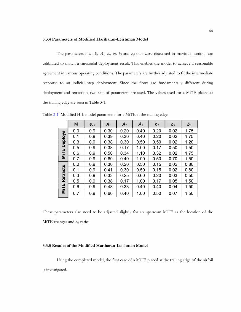
66
3.3.4 Parameters of Modified Hariharan-Leishman Model
The parameters A1, A2, A3, b1, b2, b3 and eeff that were discussed in previous sections are
calibrated to match a sinusoidal deployment result. This enables the model to achieve a reasonable
agreement in various operating conditions. The parameters are further adjusted to fit the intermediate
response to an indicial step deployment. Since the flows are fundamentally different during
deployment and retraction, two sets of parameters are used. The values used for a MiTE placed at
the trailing edge are seen in Table 3-1.
These parameters also need to be adjusted slightly for an upstream MiTE as the location of the
MiTE changes and eeff varies.
3.3.5 Results of the Modified Hariharan-Leishman Model
Using the completed model, the first case of a MiTE placed at the trailing edge of the airfoil
is investigated.
Table 3-1: Modified H-L model parameters for a MiTE at the trailing edge
M eeff A1 A2 A3 b1 b2 b3
0.0 0.9 0.30 0.20 0.40 0.20 0.02 1.75
0.1 0.9 0.39 0.30 0.40 0.20 0.02 1.75
0.3 0.9 0.38 0.30 0.50 0.50 0.02 1.20
0.5 0.9 0.38 0.17 1.00 0.17 0.50 1.50
0.6 0.9 0.50 0.34 1.10 0.32 0.02 1.75
MiTE Deploys
0.7 0.9 0.60 0.40 1.00 0.50 0.70 1.50
0.0 0.9 0.30 0.20 0.50 0.15 0.02 0.80
0.1 0.9 0.41 0.30 0.50 0.15 0.02 0.80
0.3 0.9 0.33 0.25 0.60 0.20 0.03 0.50
0.5 0.9 0.38 0.17 1.00 0.17 0.05 1.50
0.6 0.9 0.48 0.33 0.40 0.40 0.04 1.50
MiTE Retracts
0.7 0.9 0.60 0.40 1.00 0.50 0.07 1.50

67
3.3.5.1 Trailing Edge MiTE
The first case investigates the effects of trailing-edge MiTE at a low Mach number of 0.1 and
a reduced frequency of k = 0.14 (1/rev) seen in Figure 3-5.
These data show that the model agrees well with the CFD for the lift, drag, and pitching
moment at these conditions. Figure 3-6 shows results from when the reduced frequency is increased
to 0.56 (4/rev).
(a) (b)
(c)
Figure 3-5: Comparisons between CFD and modified H-L unsteady flapping model for M=0.1, α=0 deg, k=0.14 (a) lift (b) drag (c) moment [26]

68
This case again shows good agreement between the CFD and the H-L model. Next is to
compare the model with CFD when there are changes in angle of attack. To do this, the angle of
attack is set at an angle of attack of 10 degrees. The results are shown in Figure 3-7.
(a) (b)
(c)
Figure 3-6: Comparisons between CFD and modified H-L unsteady flapping model for M=0.1, α=0 deg, k=0.56 (a) lift (b) drag (c) moment [26]

69
In this case, there is good agreement between the CFD and the H-L model in terms of lift
and pitching moment. There are however slight discrepancies between the drags. This was to be
expected as it is hard to both model and experimentally measure drag especially with the cases at
hand. A high Mach number case is then investigated to see the compressibility effects. Here, the
freestream Mach number is increased to 0.6 and the results are seen in Figure 3-8.
(a) (b)
(c)
Figure 3-7: Comparisons between CFD and modified H-L unsteady flapping model for M=0.3, α=10 deg, k=0.2 (a) lift (b) drag (c) moment [26]

70
Again, the lift and pitching moment correlate well between the CFD and H-L model. The
discrepancy in drag is seen again.
Finally, the modified H-L model was used to calculate the lift amplitude while the Mach
number was varied. The results of the model, seen in Figure 3-9, show good agreement with those
predicted with CFD seen in Figure 2-23. This means that the model is capable of being used for
vibration control purposes as it captures the effects to lift from both changes in Mach number and
reduced frequency.
(a) (b)
(c)
Figure 3-8: Comparisons between CFD and modified H-L unsteady flapping model for M=0.6, α=0 deg, k=0.5 (a) lift (b) drag (c) moment [26]

71
3.3.5.2 Upstream MiTE
The model is now tested with a MiTE located upstream of the trailing edge of the airfoil.
The first case is that of a MiTE placed at 0.90c and a height of 0.02c at a Mach number of 0.45 and a
reduced frequency of k = 0.14 (1/rev).
Figure 3-9: Magnitude and phase lag vs. reduced frequency predicted using the modified H-L unsteady flapped airfoil model at various Mach numbers [26]

72
In this case, there is good agreement between the CFD and the H-L model in terms of lift
and pitching moment. There are however slight discrepancies between the drags as seen for the
trailing-edge MiTE. The reduced frequency of the MiTE deployment was increased to 0.56 (4/rev)
and the results are seen in Figure 3-11
(a) (b)
(c)
Figure 3-10: Comparisons between CFD and modified H-L unsteady flapping model of a 2% MiTE placed at 0.9c for M=0.45, α=0 deg, k=0.14 (a) lift (b) drag (c) moment

73
Again, there is good correlation between the CFD and the model for the lift and pitching
moment with some discrepancy in terms of drag. The location of the MiTE is now varied from 0.85c
to 1.00c at a freestream Mach number of 0.6 and a reduced frequency of 1.0.
(a) (b)
(c)
Figure 3-11: Comparisons between CFD and modified H-L unsteady flapping model of a 2% MiTE placed at 0.9c for M=0.45, α=0 deg, k=0.56 (a) lift (b) drag (c) moment
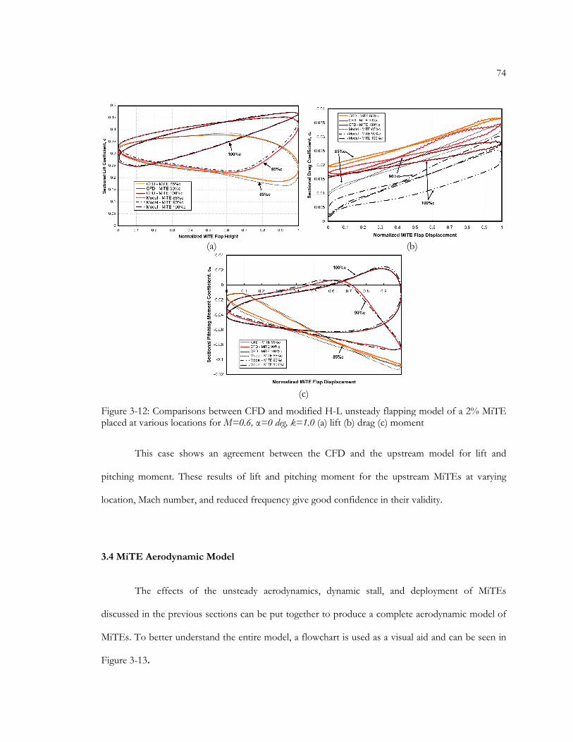
74
This case shows an agreement between the CFD and the upstream model for lift and
pitching moment. These results of lift and pitching moment for the upstream MiTEs at varying
location, Mach number, and reduced frequency give good confidence in their validity.
3.4 MiTE Aerodynamic Model
The effects of the unsteady aerodynamics, dynamic stall, and deployment of MiTEs
discussed in the previous sections can be put together to produce a complete aerodynamic model of
MiTEs. To better understand the entire model, a flowchart is used as a visual aid and can be seen in
Figure 3-13.
(a) (b)
(c)
Figure 3-12: Comparisons between CFD and modified H-L unsteady flapping model of a 2% MiTE placed at various locations for M=0.6, α=0 deg, k=1.0 (a) lift (b) drag (c) moment

75
Figure 3-13: Flowchart of MiTE Aerodynamic Model

76
Following this flowchart, the aerodynamic characteristics of a MiTE may be completely
modeled including the deployment and dynamic stall. Figure 3-14 shows the lift response of a MiTE
including the effects of dynamic stall.
The comparison of this lift response with that of the CFD results shows good correlation
and gives confidence in the MiTE model. It should be noted however that the drag results of the
CFD and that of the model do not match. This is due to the Modified Hariharan-Leishman model
failing to fully capture the initial drag rise due to the indicial step deployment of the MiTE.
Nevertheless, the overall results are satisfactory in providing a fairly accurate and efficient method in
calculating the aerodynamics of MiTEs.
Figure 3-14: Results of the MiTE Model

77
3.5 Summary
The Lesihman-Beddoes dynamic stall model was applied an airfoil with a Gurney flap to
capture the effects during dynamic stall. This model was compared with experimental results showing
the accuracy of the dynamic stall model for airfoils with and without Gurney flaps. Since the dynamic
stall models are based on static airfoil data, the baseline data sets are modified to obtain the airfoil
characteristics when using Gurney flaps throughout a full range of angles of attack and Mach
numbers by use of CFD results. Then, a modified Hariharan-Leishman unsteady flapped airfoil
model is used to calculate the unsteady aerodynamics of MiTEs. This model also includes a vortex
model to capture the effects of vortex formulation and advection of an upstream MiTE.
These models produce lift and pitching moment results that are valid for large angles of
attack, Mach numbers and varying location of the MiTE. The drag results, however, showed
discrepancies and require refinement.

Chapter 4
MiTE Rotor Performance
The application of Gurney flaps to helicopter rotors shows potential to increase the rotor
performance at high thrust levels and in forward flight. This is, however, accompanied by a reduction
in performance in low thrust and low-speed flight conditions. [48] These performance investigations
were then extended by the use of trailing-edge MiTEs. [25] These MiTEs were able to selectively
deploy along the blade span and around the azimuth of the rotor showing increases in rotor
performance throughout the flight envelope. This particular research also suggests an application to
vibration control. The current objective is to investigate the possible rotor performance
enhancements of upstream MiTEs.
4.1 ROTOR Program
The rotor performance enhancements due to MiTEs are investigated using a modified
version of ROTOR, a rotor performance analysis code based on blade-element theory.[3] This
program predicts the required power for hover and level forward flight with a trimmed rotor state.
The rotor is trimmed in the longitudinal and vertical directions as well as trimming the pitching and
rolling moments to zero. This program does not model a tail rotor, so the rotorcraft is not trimmed
in the lateral direction or yawing moment.
The inflow model used in the computer program is a non-uniform cosine downwash model.
Blade flapping with a hinge offset is also modeled although lead-lag dynamics are neglected. The
aerodynamic loads are calculated and then combined with the inertial forces. These combined forces
79
are then integrated along the span of the blade and around the azimuth to determine the rotor thrust,
torque, and power.
4.1.1 Generation of Airfoil Data Tables
In order for ROTOR to compute the aerodynamic loads, a table of airfoil force coefficients
spanning a range of angles of attack and Mach numbers is needed. For MiTE performance
calculations, two tables are needed for each airfoil. One table is needed for the baseline
characteristics and another for the airfoil equipped with a Gurney flap.
The baseline airfoil characteristics were determined through the use of MSES.[38] This
provided a consistent set of results over a range of operation of the rotor. It was used to predict cl, cd,
and cm for the baseline airfoil from positive to negative stall and at Mach numbers from 0.0 to 1.0.
The sectional characteristics are assumed to be independent of Reynolds number. This is supported
by the fact that MSES predicted transition forward of 20 percent chord over most of the operational
range. The wind tunnel tests in Chapter 2 also support these results by the small difference seen in
lift coefficients between natural and fixed transition. Therefore, transition was set to 2 percent chord
on the upper surface and 7 percent on the lower in MSES. With these characteristics of the flow, the
data generated in MSES at the Reynolds number 4.0x10⁶, which is the average value at blade mid
span around the azimuth. To generate the tables for the Gurney flapped airfoils, the ∆cl, ∆cd, and ∆cm
values from CFD were added to the baseline tables at various Mach numbers.
The ROTOR program requires airfoil data at angles of attack ranging from
oo 180180 <<− α . To obtain this needed data beyond positive and negative stall, the airfoil data
from MSES was blended into that of the NACA 0012 airfoil at high angles of attack. [49] In
situations where the airfoil is approaching stall and MSES was unable to converge, the
Kirchhoff/Helmholtz model is used to predict stall based on a combination of converged

80
predictions and the NACA 0012 data. This sort of situation usually occurs at Mach numbers greater
than the critical Mach number. In the analysis of the rotor, this data usually don’t have to be
implemented since it occurs at relatively high Mach numbers on the advancing side of the rotor
where stall is typically avoided.
4.1.2 Aerodynamic Models
4.1.2.1 Oscillating Airfoil Model
To model the aerodynamics during the rotor analyses, the models are separated into two
categories. The first category is the modeling of the baseline airfoil without a MiTE. There are three
different types of models that can be used: quasi-steady, unsteady, or dynamic stall. The quais-steady
model is based on the airfoil data and the angle of attack is based on the pitch rate, downwash, blade
flapping, and other motions. The unsteady aerodynamic model modifies the quasi-steady angle of
attack based on indicial methods as discussed in Section 3.2.1.1.
The Leishman-Beddoes dynamic stall model is used to determine additional unsteady effects
such as lags in the separation and pressure responses, and considers the effects of the leading –edge
vortices as discussed in Section 3.2.1.2. In the rotor performance code, the dynamic stall parameters
are based upon the experimental data of the NACA 0012 airfoil since data is available. This
approximation is due to the fact that the separation and pressure time constants, Tf and Tp, are
somewhat airfoil-independent parameters. For future projects where the rotor is being designed,
more appropriate constants should be selected that are more representative of the actual airfoil.
81
4.1.2.2 Oscillating MiTE Model
The second category of aerodynamic models is one that pertains to the modeling of MiTEs.
The program is set up to use a separate set of data that represents the same airfoil with the specific
Gurney flap being used attached to the airfoil. This provides the needed GFlc ,∆ and GFdc ,∆ as a
function of angle of attack and Mach number.
The user has the ability to select a steady linear model or unsteady flapped airfoil model. The
linear model assumes there are no lags and uses linear interpolations between the baseline and the
Gurney flap data sets. This is based on the instantaneous height of the MiTE.
The unsteady flapped airfoil model incorporates the model found in Section 3.3 into the
rotor performance code. The model adds the unsteady effects of the motion of the MiTE. This
determines the lead and lag of the system and its effects overall. The effects of the upstream MiTEs,
where there is the formulation and advection of vortices on the lower surface of the airfoil, are also
accounted for.
4.1.3 MiTE Deployment Scheme
The primary use of MiTEs in this research is stall alleviation as a means to increase rotor
performance. The objective is initially to have the MiTE retracted at lower angles of attack when
additional lift is not needed. When the lift requirements increase, MiTEs deploy to achieve higher lift
without a stall drag penalty. The MiTE remains deployed as need to provide additional lift and then
retracts when the lift-to-drag ratio drops below that of the baseline airfoil. The deployment schedule
the MiTE is shown in Figure 4-1.
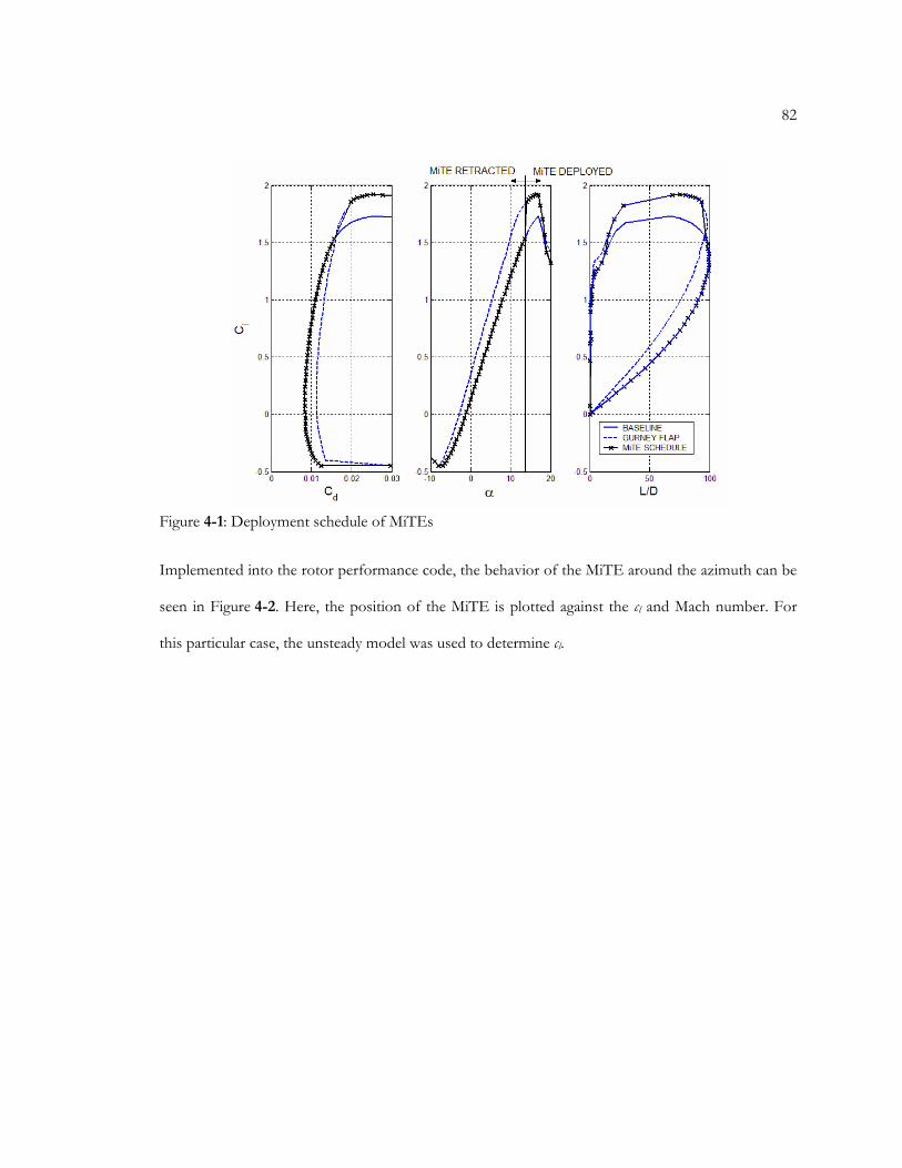
82
Implemented into the rotor performance code, the behavior of the MiTE around the azimuth can be
seen in Figure 4-2. Here, the position of the MiTE is plotted against the cl and Mach number. For
this particular case, the unsteady model was used to determine cl.
Figure 4-1: Deployment schedule of MiTEs

83
4.2 Rotor Performance Analysis
The rotor performance comparisons are based upon the Boeing/Sikorsky RAH-66
Comanche helicopter. The rotor blades utilize the VR-12 airfoil on the inboard sections and
transition to a SSC-A09 airfoil on the outboard sections. As the break point for the airfoil sections
was not published, it was assumed to be located at r/R=0.75. Table 4-1 shows the other parameters
of the RAH-66 Comanche used in the performance analysis.
Figure 4-2: MiTE height and cl variations around the rotor azimuth

84
The MiTE used in these studies is located at 0.90c and has a height of 0.02c. They are also
assumed to span the entire span of the blade. The dynamic stall model and the unsteady flapped
airfoil model is used in performance predictions. This is done to capture as much of the effects as
possible of the lower surface vortex associated with the upstream MiTE.
4.2.1 Importance of Unsteady Modeling
In previous research of trailing-edge MiTEs, the linear interpolation model was used to
determine the effects of MiTEs, since there is only a small difference between it and the unsteady
model. As shown in Figure 4-3, this is not the case with an upstream MiTE, for which the required
power of rotor over a range of advance ratios is influenced by the use of the unsteady MiTE model.
Table 4-1: RAH-66 Comanche Characteristics
Parameter Value
Number of Blades 5
Rotor Diameter 40 ft
Hub Radius 2.5 ft
Hinge Offset 1.5 ft
Blade Chord 1.1 ft
Linear Twist -8.5 deg
Tip Speed 700 ft/s
Blade Weight 2.9 lb/ft
Equiv. Flat Plate Drag 18 ft2
Base Weight 10600 lb

85
This dictates that the unsteady aerodynamic model should be modeled to capture the additional
power required by the rotor.
Another aspect of the rotor that is affected by the aerodynamic model chosen is that of the
MiTE deployment around the azimuth. Figure 4-4 shows a MiTE deployment comparison of a rotor
in high speed flight (µ = 0.4) using the quasi-steady model versus the dynamic stall with the unsteady
MiTE model. Here, MiTEs are fitted to the outboard airfoil only and deployed as indicated by the
MiTE is deployed in the shaded region. Again, sizable differences are seen between the two cases as
to where the MiTE deploys and retracts.
Figure 4-3: Power Required Comparison

86
4.2.2 Pitching Moment Concern
A major concern in the rotorcraft community concerning rotor blades is that of the pitching
moment. Due to the concern over pith-link loads in dynamic stall, the pitching moment needs to be
kept to a minimum. The pitching moment coefficient does increase as MiTEs are deployed, but
whether or not the moment actually increases depends on where on the rotor, in span and azimuth,
the MiTEs are located. If the load is beyond the limits of the blade, MiTEs will not be able to be
used. Figure 4-5 shows the maximum pitching moment on each side of the rotor over a range of
advance ratios. These are normalized by the maximum pitching moment on the advancing side of the
rotor, which is taken to be the limiting case. It is seen that even with the MiTEs fully deployed in
hover, the pitching moment is still lower than the limiting case.
(a) (b)
Figure 4-4: MiTE deployment on rotor disk at µ = 0.4 (a) quasi-steady (b) dynamic stall w/ unsteady MiTE

87
4.2.3 Forward Speed Performance
In previous research, it has been shown that MiTEs are capable of increasing the maximum
speed of the rotorcraft.[25] This is consequence of a MiTE’s ability to delay stall on the retreating
blade. This reduced drag and increased the lift-to-drag ratio allows greater speeds. It was also
demonstrated that the greatest effect is due to the increased its maximum lift on the transonic airfoil.
Hartwich also showed that changing the airfoil distribution across the blade had the possibility of
increasing the maximum speed of the rotorcraft.[3] It was therefore decided to explore changing the
airfoil distribution on the rotor of the Comanche and use MiTEs along the span of the blade to
produce a greater maximum speed. The results can be seen in Figure 4-6
Figure 4-5: Blade Maximum Pitching Moment

88
Starting at the initial radial transistion of r/R=0.75, the use of the SSC-A09 transonic airfoil
was increased by moving the breakpoint inboard. This reduced the compressibility drag on the
advancing blade by the increasing use of the transonic airfoil and alleviating stall on the retreating
blade with use of the MiTEs. The maximum speed gradually increased from 175 kts to 210 kts before
the speed decreasing again, a consequence of increased retreating blade stall. This increase shows a
possible increase of 20 percent in the maximum forward speed of the Comanche.
4.2.4 Maximum Altitude Performance
Another scenario involves increase use of the inboard airfoil, the VR-12, and MiTEs that
span the length of the rotor blade to increase the service ceiling of the Comanche helicopter. The
same method was used as in the maximum speed case, where the radial transition point is moved on
Figure 4-6: Maximum Speed Increase of the Comanche

89
the rotor blade. This time however, instead of moving the transition point inboard, its moved
outboard. The results are seen in Figure 4-7.
Here, the rotor benefits from the additional cl of both the rotor and the MiTE. As was
expected, the radial distribution moved outboard to the tip. The service ceiling increased from 14,980
ft to 16180 ft, an increase of 8 percent.
4.3 Advanced Designs
Although large gains in performance have been seen in these studies, there is potential for
even greater gains. The following are few areas that can room for improvement in order to optimize
the performance of MiTEs.
Figure 4-7: Service Ceiling Increase of Comanche

90
4.3.1 Rotors Designed with MiTEs
One area that has potential to produce large gains in performance through the use of MiTEs
is that of geometric configuration. All of the situations analyzed in this research used existing rotors.
Clearly, additional gains could be achieved if a rotor was designed utilizing MiTEs from the onset.
Sections 4.2.3 and 4.2.4 did preliminary investigations into this and showed the potential increases
possible through the use of MiTEs and by changing the existing airfoil distribution along the span of
the blade.
Another potential area of improvement is inthe design of airfoils used on the rotor blades.
Up until now, rotorcraft airfoils have been selected based upon their static characteristics. It was seen
in Chapter 2 that the unsteady characteristics of the airfoils did not necessarily correlate well with the
static characteristics. It would then be very beneficial to investigate the design of airfoils for an
unsteady environment and the use of MiTEs. This possibly has the potential of performance increase
above those seen here in this research.
4.3.2 Deployment Schemes
The MiTE deployment scheme used was that of deploying when more cl is needed to avoid
stall and retracting once the lift-to-drag ratio was less than that of the baseline airfoil. Initially, an
instantaneous deployment scheme was used. This deployment schedule was smoothed to produce a
model that accounts for realistic deployment time.
Currently, there are other research efforts underway that are tailoring the lift over the rotor
to produce an optimal distribution and reduce the induced power requirements. These require a
deployment scheme that is capable of a partial deployment of a MiTE, something that is not possible
with the current deployment scheme, but is easily attainable.

91
4.4 Summary
The use of upstream MiTE was investigated for the performance enhancement and
extension of the flight envelope for rotorcraft. Using the rotor performance code ROTOR, the
importance of unsteady aerodynamics modeling was shown by the difference in power requirements
between the models. Furthermore, the difference in MiTE deployment was shown with the unsteady
case having greater use of MiTEs over the azimuth of the rotor disk. The issue of increased pitching
moment on the blades due to MiTE deployment was shown not to be an issue. This was shown by
that the fact the pitching moment increase due to MiTEs is less than that of the baseline airfoil on
the advancing blade during high speed flight.
As for performance enhancements, the RAH-66 Comanche helicopter was used as the
model helicopter. It was shown that using MiTEs and altering the airfoil distribution on the rotor
yielded large increases in maximum speed. A large increase of 8 percent in service ceiling altitude was
achieved by again altering the airfoil distribution and the use of MiTEs. Further improvements are
possible by a number of methods such as the design of airfoils on the rotor and different deployment
schemes of the MiTEs.

Chapter 5
Conclusion
5.1 Summary of Results
MiTEs place at the trailing edge and upstream of the trailing edge have been shown to be an
effective rotor performance enhancement device. A series of experimental, numerical, and analytical
investigations of MiTEs support this and show the aerodynamic potential.
5.1.1 Wind Tunnel Experiments
Both of the experiments presented in Chapter 2 investigated the aerodynamic characteristics
of the passive form of MiTEs, the Gurney flap. The first wind tunnel experiment was a static wind
tunnel test at the Penn State Low-Speed, Low-Turbulence Wind Tunnel where the Gurney flap
varied in height and chord-wise locations. They were found to provide similar lift increases upstream
of the trailing edge of the airfoil. It was found, however, that performance penalties were incurred
when the Gurney flap was moved forward.
The second wind tunnel experiment took place at NASA Ames’ Compressible Dynamic Stall
Facility and analyzed an oscillating airfoil. This experiment had a Gurney flap on the model and
showed similar aerodynamic effects through dynamic stall as were shown in the static experiment. At
higher coefficients of lift, the Gurney flap increased the aerodynamic efficiency and demonstrated the
ability to decrease the pitching moments at which the baseline airfoil stalls.

93
5.1.2 CFD Investigations
MiTEs were investigated using the CFD program OVERFLOW2. These studies involved
MiTEs placed at the trailing edge and upstream of the trailing edge. The results showed that the
chordwise location of the MiTE greatly affected the unsteady aerodynamics. When MiTEs are place
at the trailing-edge, the results agree with unsteady aerodynamic theories that are valid for plain flaps.
As the MiTE was moved upstream, strong vortical flows were created on the lower surface of the
airfoil. This vortex caused delays in the development of lift and large phase lags between the resulting
aerodynamic forces and MiTE deployment position. This also showed possible decreases in the
airfoil’s sectional performance characteristics at high deployment frequencies and low speeds.
Nevertheless, CFD showed that MiTEs delay stall to significantly higher lift coefficients. These
qualities make these devices highly desirable on rotorcraft for performance enhancement and
vibration control.
5.1.3 Aerodynamic Modeling
The Leishman-Beddoes unsteady aerodynamics and dynamic stall models were used to
model the effects of dynamic stall of an airfoil with Gurney flaps. The model was compared with
experimental results from the NASA Ames test and showed good correlation between the two sets
of data. For the baseline airfoil characteristics, MSES was used and then the addition effects of the
Gurney flaps were determined from the CFD data all throughout a range of angles of attack and
Mach numbers.
For MiTEs placed at the trailing-edge, a modified version of the Hariharan-Leishman
unsteady flapped airfoil model was used to capture the unsteady aerodynamics of a MiTE
deployment. This model was further modified for MiTEs located upstream of the trailing edge by
modeling the lower surface vortex and associated phase lags. The results of this model are also in

94
agreement with those of the CFD data for both lift and pitching moment, although discrepancies in
drag show the need for more research. The unsteady aerodynamic model, dynamic stall model, and
unsteady flapped airfoil model were then coupled and showed good agreement with CFD to model
MiTEs in dynamic stall.
5.1.4 MiTE Rotor Performance
The aerodynamic models were implemented into a blade-element rotor performance code to
investigate the effects of MiTEs on rotorcraft. The model helicopter used was the Boeing/Sikorsky
RAH-66 Comanche and the rotor blades utilized MiTEs placed upstream of the trailing edge. First,
the importance of unsteady aerodynamic modeling was investigated. This showed differences in both
power required and MiTE deployment around the azimuth of the rotor confirming the need for
adequate unsteady modeling. The pitching moment of MiTEs was investigated and showed that
MiTEs did not exceed the pitching moment seen on baseline rotor blades during forward flight. It
was also shown that the maximum forward speed and service ceiling can be increased through the
use of MiTEs and varying the airfoil distribution along the span of the rotor blade.
5.2 Conclusions
With the results presented of MiTEs placed upstream of the trailing edge, there are
numerous applications to rotorcraft. Segmenting the devices along the span of the blade would
provide azimuthal control of the lift distribution for minimizing induced drag, vibration control and
increasing rotor performance. All of these benefits would be realized with a device that possess
actuation loads many orders of magnitude less than conventional individual blade control systems.

List of References
1. Leishman, J. G., Principles of Helicopter Aerodynamics, 2nd Edition, Cambridge University Press, New York, NY, 2006.
2. Dadone, L.. “Rotor Airfoil Optimization: An Understanding of the Physical Limits,” presented at the AHS 34th Annual Forum, Washington, D.C., May 1978.
3. Hartwich, R., “Parametric Study for the Design of Advanced Rotorcraft Airfoils,” M.S.Thesis, Dept. of Aerospace Engineering, Penn State University, University Park, PA, December 1999.
4. Sloof, J.W., Wortmann, F.X., Duhon, J.M., “The Development of Transonic Airfoils for Helicopter.” AHS 31st Annual Forum, Washington, D.C., May 1975.
5. Blackwell, J.A., Hinson, B.L., “The Aerodynamic Design of an Advanced Rotor Airfoil,” Advanced Technology Airfoil Research, Vol. 2, NASA Conference Publication 2046, March 1978.
6. De la Cierva, J., and Rose, D., Wings of Tomorrow: The Story of the Autogiro, Brewer, Warren & Putnam, New York, 1931.
7. Beavan, J.A., and Lock, C. N. H., “The Effect of Blade Twist on the Characteristics of the C-30 Autogyro,” Aeronautical Research Council R&M 1727, 1939.
8. Leishman, J. G., The Helicopter: Thinking Forward, Looking Back, College Park Press, College Park, MD, 2007.
9. Prouty, R. W., Helicopter Performance, Stability and Control. Krieger Publishing, Malabar, Florida, 1990.
10. Department of the Army, “1998 Army Science and Technology Master Plan, Rotary Wing Vehicle (RWV) Technology Development Approach (TDA),” 1998.
11. Joslin, R.D., “Aircraft Laminar Flow Control,” Annual Review of Fluid Mechanics, Vol. 30, No. 198, 1998.
12. Amitay, M., Smith, B.L., and Glezar, A., “Aerodynamic Flow Control Using Synthetic Jet Technology,” AIAA Paper 98-0208, 36th Aerospace Sciences Meeting and Exhibit, Reno, NV, January 12-15, 1998.
13. Replace with Bibliography Entry TextMaughmer, M., Lesieutre, G., Thepvongs, S., Anderson, W, Kinzel, M., “Miniature Trailing-Edge Effectors for Rotorcraft Applications”, AHS 59th Forum and Technology Display, Phoenix, AZ, May 2003.
14. Lee, H., Kroo, I.M., "Computational Investigation of Airfoils with Miniature Trailing Edge Control Surfaces ," AIAA Paper 2004-1051, January 2004.
96
15. Standish, K.J., Van Dam, C.P., “Computational Analysis of a Microtab-Based Aerodynamic Load Control System for Rotor Blades,” American Helicopter Society Aeromechanics Specialists' Conference, San Francisco, CA, January 2004.
16. Yen Nakafuji,D.T, van Dam , C.P., Smith, R.L., Collins, S.D., "Active Load Control for Airfoils using Microtabs," Journal of Solar Energy Engineering, November 2001 Volume 123, Issue 4, pp. 282-289.
17. Howard, K., "Gurney Flap," Motorsport Magazine, September 2000, U.K.
18. Liebeck, R.H., “Design of Subsonic Airfoils for High Lift,” Journal of Aircraft, Vol. 15, No. 9, September 1978, pp547-561.
19. Giguére, P., Lemay, J., Dumas, G., "Gurney Flap Effects and Scaling for Low-Speed Airfoils," AIAA Paper 95-1881, 13th AIAA Applied Aerodynamics Conference San Diego, June 1995.
20. Jeffery, D.R.M. and Hurst, D.W., “Aerodynamics of the Gurney Flap,” AIAA Applied Aerodynamic Conference, AIAA 96-2418-CP, 1996.
21. Jeffrey, D., Zhang, X., Hurst, D.W., “Aerodynamics of Gurney Flaps on a Single-Element High-Lift Wing,” Journal of Aircraft, Vol. 37, March-April 2000, pp. 295-301.
22. Zerihan, J. and Zhang, X., “Aerodynamics of Gurney flaps on a wing in ground effect,” AIAA J., Vol. 39, No. 5, July 2001, pp. 772-780.
23. Richter, K. and Rosemann, H., “Experimental investigation of trailing-edge devices at transonic speeds,” The Aeronautical Journal, April 2002, pp. 185-193.
24. Bechert, D.W., Meyer, R., Hage, W., “Drag Reduction of Airfoils with Miniflaps. Can We Learn From Dragonflies?” AIAA-2000-2315, June 19-22, 2000, Denver, CO.
25. Selig M., Lyon C., Giguére P., Ninham C., and Guglielmo J., Summary of Low-Speed Airfoil Data, Vol. 2, SoarTech Publ., Virginia Beach, VA, 1996.
26. Kinzel, M., Maughmer, M.D. and Lesieutre, G.A., "Miniature Trailing-Edge Effectors for Rotorcraft Performance Enhancements," Journal of the American Helicopter Society, Vol. 52,(2), April 2007, pp. 146-158.
27. Kentfield, J.A.C., “The Potential of Gurney Flaps for Improving the Aerodynamic Performance of Helicopter Rotors,” AIAA International Powered Lift Conference, pp. 283-292, AIAA Paper 93-4883, 1993.
28. Bieniawski, S. and Kroo, I.M., “Flutter Suppression Using Micro-Trailing Edge Effectors,” AIAA Paper 2003-1941, 2003.
29. Brophy, C.M., “Turbulence Management and Flow Qualification of The Pennsylvania State
University Low Turbulence, Low Speed, Closed Circuit Wind Tunnel,” M.S. Thesis, Department of Aerospace Engineering, Penn State University, University Park, PA, 1993.

97
30. Prankhurst, R.C. and Holder, D.W., Wind-Tunnel Technique, Sir Isaac Pitman & Sons, Ltd, London, 1965.
31. Allen, H.J., and Vincenti, W.G., “Wall Interference in a Two-Dimensional-Flow Wind Tunnel, With Consideration of the Effect of Compressibility,” NACA Report 782, 1944.
32. Somers, D.M., “Effects of Airfoil Thickness and Maximum Lift Coefficient on Roughness
Sensitivity,” Airfoils, Incorporated, October, 1998. 33. Dadone, L.U., “Future Directions in Helicopter Rotor Development,” American Helicopter
Society Aeroacoustics Specialists’ Meeting, Arlington, Texas, February 25-27, 1987.
34. Braslow, A.L. and Knox, E.C., “Simplified Method for Determination of Critical Height of Distributed Roughness Particles for Boundary-Layer Transition at Mach Numbers From 0 to 5,” NACA TN 4363, 1958.
35. Maughmer, M.D. and Bramesfeld, G., “An Experimental Investigation of Gurney Flaps.” Journal of Aircraft, (To Appear in 2008)
36. Martin, P.B., McAlister, K..W., Chandrasekhara, M.S., Geissler, W., "Dynamic Stall Measurements and Computations for a VR-12 Airfoil with a Variable Droop Leading Edge," AHS 59th Forum and Technology Display, Phoenix, AZ, May 2003.
37. Carr, L.W., Chandrasekhara, M.S., "Design and Development of a Compressible Dynamic Stall Facility," Journal of Aircraft, Vol. 29, No. 3, May 1992, pp314-318.
38. Chandrasekhara, M.S., Martin, P.B., Tung, C. "Compressible Dynamic Stall Performance of a Variable Droop Leading Edge Airfoil with a Gurney Flap," AIAA 2004-0041, January 2004.
39. Drela, M., “A User's Guide to MSES 3.04,” Cambridge, MA, Sept. 2002.
40. Buning, P. G., Jespersen, D. C., Pulliam, T. H., Chan, W. M., Slotnick, J. P., Krist, S. E., Renze, K. J., ``OVERFLOW User's Manual, Version 1.8,'' NASA Langley Research Center, Hampton, VA, 1998.
41. Meakin, B. and Potsdam, M., “Reference Guide for Scalable OVERLOW-D, v1.5e” NASA Ames Research Center, June 2002.
42. Spalart P.R., Allmaras S. R., "A One-Equation Turbulence Model for Aerodynamic Flows," AIAA 92-0439, AIAA 29th Aerospace Sciences Meeting, Reno, Nevada, Jan. 1992.
43. Theodorsen, T., “General Theory of Aerodynamic Instability and the Mechanism of Flutter,” NACA Report 496. 1935.
44. Leishman, J.G., Beddoes, T.S., "A Semi-Empirical Model for Dynamic Stall," Journal of the
American Helicopter Society, Vol. 34, No. 3, July 1989, pp. 3-17.
45. Johnson, W., “Rotorcraft Aerodynamic Models for Comprehensive Analysis,” presented at the AHS 54th Annual Forum, Washington, DC, May 1998.
98
46. Leishman, J. G., Beddoes, T. S., "A Generalized Model for Airfoil Unsteady Aerodynamic Behavior and Dynamic Stall using the Indicial," presented at the 42nd Annual Forum of the American Helicopter Society, Washington, D.C., June 1986.
47. Hariharan, N., and Leishman, J. G., “Unsteady Aerodynamics of a Flapped Airfoil in
Subsonic Flow by Indicial Concepts,” Journal of Aircraft, Vol. 33, No. 5, Sep.- Oct. 1996, pp. 855 868.
48. Leishman, J.G., "Unsteady Lift of a Flapped Airfoil by Indicial Concepts," Journal of Aircraft, Vol. 31, No. 2, March-April. 1994, pp. 288-297.
49. Kentfield, J.A.C., “The Potential of Gurney Flaps for Improving the Aerodynamic Performance of Helicopter Rotors,” AIAA International Powered Lift Conference, pp. 283-292, AIAA Paper 93-4883, 1993.
50. Critzos, C.C., Heyson, H.H., and Boswinkle, R.W., “Aerodynamic Characteristics of NACA 0012 Airfoil Section at Angles of Attack from 0° to 180°,” NACA TN 3361’ 1955.