the pennsylvania state university the graduate school college of

The Pennsylvania State University

The Graduate School

College of Engineering

ROBUST-ADAPTIVE ACTIVE VIBRATION CONTROL OF ALLOY AND

FLEXIBLE MATRIX COMPOSITE ROTORCRAFT DRIVELINES VIA

MAGNETIC BEARINGS: THEORY AND EXPERIMENT

A Thesis in

Mechanical Engineering

by

Hans A. DeSmidt

2005 Hans A. DeSmidt

Submitted in Partial Fulfillmentof the Requirements

for the Degree of

Doctor of Philosophy

May 2005

The thesis of Hans A. DeSmidt was reviewed and approved* by the following:

Kon-Well WangWilliam E. Diefenderfer Chaired Professor in Mechanical EngineeringThesis Co-AdvisorCo-Chair of Committee

Edward C. SmithProfessor of Aerospace EngineeringThesis Co-AdvisorCo-Chair of Committee

Charles E. BakisProfessor of Engineering Science and Mechanics

Christopher D. RahnProfessor of Mechanical Engineering

A. Scott LewisDual Research Associate of Applied Research Lab and Mechanical Engineering

Richard C. BensonProfessor of Mechanical EngineeringHead of the Department of Mechanical Engineering

* Signatures are on file in the Graduate School.

iii

ABSTRACT

This thesis explores the use of Active Magnetic Bearing (AMB) technology and

newly emerging Flexible Matrix Composite (FMC) materials to advance the state-of-the-

art of rotorcraft and other high performance driveline systems. Specifically, two actively

controlled tailrotor driveline configurations are explored. The first driveline configuration

(Configuration I) consists of a multi-segment alloy driveline connected by Non-Constant-

Velocity (NCV) flexible couplings and mounted on non-contact AMB devices. The

second configuration (Configuration II) consists of a single piece, rigidly coupled, FMC

shaft supported by AMBs. For each driveline configuration, a novel hybrid robust-

adaptive vibration control strategy is theoretically developed and experimentally

validated based on the specific driveline characteristics and uncertainties. In the case of

Configuration I, the control strategy is based on a hybrid design consisting of a PID

feedback controller augmented with a slowly adapting, Multi-Harmonic Adaptive

Vibration Control (MHAVC) input. Here, the control is developed to ensure robustness

with respect to the driveline operating conditions e.g. driveline misalignment, load-

torque, shaft speed and shaft imbalance. The analysis shows that the hybrid PID/MHAVC

control strategy achieves multi-harmonic suppression of the imbalance, misalignment and

load-torque induced driveline vibration over a range of operating conditions.

Furthermore, the control law developed for Configuration II is based on a hybrid robust

H∞ feedback/Synchronous Adaptive Vibration Control (SAVC) strategy. Here, the effects

of temperature dependent FMC material properties, rotating-frame damping and shaft

imbalance are considered in the control design. The analysis shows that the hybrid

H∞/SAVC control strategy guarantees stability, convergence and imbalance vibration

suppression under the conditions of bounded temperature deviations and unknown

imbalance. Finally, the robustness and vibration suppression performance of both new

AMB driveline configurations is experimentally confirmed using a frequency-scaled

AMB driveline testrig specifically developed for this research.

iv

TABLE OF CONTENTS

LIST OF FIGURES .....................................................................................................viii

LIST OF TABLES.......................................................................................................xv

ACKNOWLEDGMENTS ...........................................................................................xvii

Chapter 1 INTRODUCTION.....................................................................................1

1.1 Supercritical Rotorcraft Drivelines................................................................11.2 Non-Constant Velocity Couplings ................................................................61.3 Aerodynamic Loading ...................................................................................111.4 Composite Shafting .......................................................................................121.5 Active Magnetic Bearings .............................................................................141.6 Closed-Loop Active Vibration Control of Flexible Shafts............................171.7 Thesis Objectives...........................................................................................22

Chapter 2 DEVELOPMENT OF SEGMENTED SUPERCRITICALROTORCRAFT DRIVELINE-FUSELAGE MODEL.............................27

2.1 Introduction ...................................................................................................272.2 System Description........................................................................................272.3 Flexible Shaft/NCV Coupling Kinematics....................................................302.4 Misaligned Tailrotor Driveline Kinematics...................................................252.5 Energy and Dissipation Functions.................................................................392.6 Loading Conditions and Virtual Work Expressions......................................442.7 Finite Element Formulation and Equations-of-Motion .................................492.8 Modal Reduction ...........................................................................................542.9 Magnetic Bearings.........................................................................................55

Chapter 3 STABILITY ANALYSIS OF A SEGMENTED SUPERCRITICALDRIVELINE WITH NCV COUPLINGS SUBJECT TOMISALIGNMENT AND TORQUE.........................................................58

3.1 Introduction ...................................................................................................583.2 Driveline Non-Dimensional Equations-of-Motion........................................593.3 Stability Analysis...........................................................................................67

v

3.3.1 Nominal System Stability.....................................................................673.3.2 Full system stability..............................................................................693.3.3 Bending-Bending Parametric Instability ..............................................743.3.4 Torsion-Bending Parametric Instability ...............................................76

3.4 Stability Analysis Summary and Conclusions ..............................................78

Chapter 4 CONFIGURATION I: ROBUST ADAPTIVE VIBRATIONCONTROL OF MISALIGNED SUPERCRITICAL DRIVELINEWITH MAGNETIC BEARINGS .............................................................81

4.1 Introduction ...................................................................................................814.2 Segmented AMB-NCV Driveline System.....................................................834.3 Active Control Law Structure .......................................................................874.4 Robust PID-MHAVC Controller Design ......................................................95

4.4.1 Step I, Robust PID Feedback Design ...................................................964.4.2 Step II, Robust MHAVC Design..........................................................99

4.5 PID-MHAVC Performance Analysis ............................................................1034.5.1 Steady-State Performance ....................................................................1044.5.2 Time-Domain Simulation.....................................................................111

4.6 Configuration I Control Law Summary and Conclusions.............................117

Chapter 5 CONFIGURATION II: ROBUST ADAPTIVE VIBRATIONCONTROL OF FLEXIBLE MATRIX COMPOSITE DRIVELINESVIA MAGNETIC BEARINGS ................................................................120

5.1 Introduction ...................................................................................................1205.2 AMB-FMC Driveline System .......................................................................1225.3 Active Control Structure................................................................................1265.4 Control Synthesis...........................................................................................1315.5 Nominal System Closed-Loop Analysis .......................................................1345.6 Closed-Loop Analysis with Shaft Temperature Deviations..........................1375.7 Configuration II Active Control Summary and Conclusions ........................141

Chapter 6 AMB/SUPERCRITICAL TAILROTOR DRIVELINE-FUSELAGETESTRIG DESIGN AND EXPERIMENTAL SETUP............................143

6.1 Introduction ...................................................................................................1436.2 Driveline Testrig Overview...........................................................................1436.3 Active Magnetic Bearings .............................................................................1516.4 Flexible Matrix Composite Shaft ..................................................................1546.5 System Inputs and Outputs............................................................................154

Chapter 7 EXPERIMENTAL INVESTIGATION ....................................................156

7.1 Introduction ...................................................................................................1567.2 NCV-Driveline Model Validation.................................................................157

vi

7.3 Active Controller Experimental Implementation ..........................................1657.3.1 PID Feedback Control Implementation................................................1677.3.2 Harmonic Adaptive Control Implementation.......................................171

7.4 Experimental Results: Configuration I with PID-MHAVC Control .............1797.5 Experimental Results: Configuration II with PID-SAVC Control................1847.6 Experimental Investigation Summary and Conclusions................................190

Chapter 8 CONCLUSIONS AND RECOMMENDATIONS FOR FUTUREWORK ......................................................................................................193

8.1 Summary and Conclusions ............................................................................1938.2 Recommendations for Future Work ..............................................................196

BIBLIOGRAPHY........................................................................................................201

Appendix A FINITE ELEMENT MODEL ELEMENTAL MATRICES .................211

A.1 Shaft Elemental Matrices ..............................................................................211A.2 Fuselage-Beam Elemental Matrices ..............................................................212

Appendix B MISALIGNMENT-INDUCED INERTIA LOAD AND TORQUELOAD PERIODIC NCV COUPLING TERMS ...................................214

B.1 Load-Inertia NCV Terms ..............................................................................214B.2 Load-Torque NCV Terms .............................................................................226

Appendix C NON-DIMENSIONAL SYSTEM MATRICES FORCONVENTIONAL DRIVELINE .........................................................229

C.1 Non-Dimensional Nominal System Matrices................................................229C.2 Non-Dimensional Load-Inertia NCV Terms.................................................230C.3 Non-Dimensional Load-Torque NCV Terms................................................234

Appendix D LEAST-SQUARES FORMULATION OF ADAPTIVE CONTROLUPDATE LAW .....................................................................................236

Appendix E ADAPTIVE CONTROL CONVERGENCE CONDITION .................238

Appendix F FMC SHAFT LAYUP AND EQUIVALENT MATERIALPROPERTIES .......................................................................................240

Appendix G EXPERIMENTAL RESULTS .............................................................243

vii

G.1 Configuration I Experimental Results ...........................................................243G.1.1 Configuration I Time-Domain Results ................................................244G.1.2 Configuration I Frequency-Domain Results........................................252

G.2 Configuration II Experimental Results..........................................................257G.2.1 Configuration II Time-Domain Results...............................................257G.2.2 Configuration II Frequency-Domain Results ......................................261

viii

LIST OF FIGURES

Fig. 1.1: Conventional supercritical tailrotor driveline and fuselage...........................2

Fig. 1.2: Common NCV coupling, 4-bolt metal disk coupling....................................6

Fig. 1.3: Boeing AH-64 coupled tailrotor driveline-fuselage mode. ...........................12

Fig. 1.4: 8-Pole attractive radial magnetic bearing. .....................................................15

Fig. 1.5: AMB-shaft digital control system. ................................................................17

Fig. 1.6: AMB-Tailrotor driveline full state feedback optimal controller. ..................20

Fig. 1.7: Closed-loop hanger bearing loads and gap displacements in forward-flight. .............................................................................................................21

Fig. 1.8: Conventional and new actively controlled driveline configurations.............24

Fig. 2.1: Segmented, multi-coupling, driveline on flexible fuselage structure............28

Fig. 2.2: Fixed-frame and rotating frame elastic deflections of shaft cross-section. ...29

Fig. 2.3: Pth NCV coupling connecting statically misaligned, flexible shafts. ............31

Fig. 2.4: NCV Coupling: U-Joint with two Euler angles α and β. ..............................32

Fig. 2.5: b in terms of i-1th shaft kinematic variables and coupling Euler angles. ...33

Fig. 2.6: b in terms of ith shaft kinematics variables and static misalignments. .......34

Fig. 2.7: Driveline static misalignment due to aerodynamic load; side-view..............36

Fig. 2.8: Driveline static misalignment due to aerodynamic load; top-view. ..............37

Fig. 2.9: Aerodynamic loads on tailrotor driveline-fuselage structure. .......................45

Fig. 2.10: Cross-section of ith shaft with mass imbalance. ..........................................47

ix

Fig. 2.11: Shaft geometric imperfection: initially bent shaft. ......................................48

Fig. 2.12: jth beam-rod-torsion finite element of the ith structure...............................50

Fig. 2.13: 8-pole radial AMB with bias and control currents. .....................................55

Fig. 3.1: Segmented driveline connected by U-joint couplings...................................60

Fig. 3.2: Nominal system whirl stability behavior.......................................................68

Fig. 3.3: Misalignment-shaft speed instability region, τ = 0.0. ...................................71

Fig. 3.4: Misalignment-shaft speed instability region, τ = 0.5τmax. .............................73

Fig. 3.5: Effect of damping on misalignment induced.................................................75

Fig. 3.6: Effect of damping on torque induced bending-bending instability. .............75

Fig. 3.7: Effect of damping, torque and misalignment on 1st torsion-bendinginstability cd = 0.0, cd = 0.04 (a) τ = 0.0; (b) τ = 0.25τmax; (c) τ = 0.5τmax; (d) τ = τmax ...........................................................................................77

Fig. 3.8: Effect of damping, torque and misalignment on 2nd torsion-bendinginstability. cd = 0.01, cd = 0.2 (a) τ = 0.0; (b) τ = 0.25τmax; (c) τ = 0.5τmax; (d) τ = τmax ...........................................................................................77

Fig. 4.1: Configuration I: segmented driveline with AMBs and NCV couplings. ......84

Fig. 4.2: Driveline with hybrid PID/Multi-Harmonic Adaptive Vibration Control. ...88

Fig. 4.3: Robust stability index, SPID vs. kp and kd with kI. = 1000 Amp/m-sec. .......97

Fig. 4.4: MHAVC Convergence Metric vs. shaft speed for weff = 0 and weff =1000; (a) [TL = 0.5TLmax, θ = 4°]; (b) [TL = TLmax, θ = 4°]. ...........................101

Fig. 4.5: θ - Ω0 MHAVC convergence regions for various weff with max0 LL TT ≤≤ . ..102

Fig. 4.6: MHAVC Robust Convergence Metric vs. MHAVC control effortweighting. ......................................................................................................103

Fig. 4.7: PID-MHAVC/AMB-driveline converged response; worst-case vibration. ..105

Fig. 4.8: PID-MHAVC/AMB-driveline response; worst-case control current............105

Fig. 4.9: PID-MHAVC/AMB-driveline response; RMS shaft vibration.....................107

x

Fig. 4.10: PID-MHAVC/AMB-driveline response; RMS control current. .................107

Fig. 4.11: PID-MHAVC/AMB-driveline vibration harmonics at AMB1....................108

Fig. 4.12: PID-MHAVC/AMB-driveline control current harmonics at AMB1. .........109

Fig. 4.13: Peak vibration amplitude at the AH-64 shaft operating speed. ...................110

Fig. 4.14: Peak AMB control current at the AH-64 shaft operating speed..................111

Fig. 4.15: PID-MHAVC controlled AMB-driveline system. ......................................112

Fig. 4.16: Real-time Harmonic Fourier Coefficient calculator block..........................112

Fig. 4.17: Multi-Harmonic Adaptive Vibration Control synthesis block. ...................113

Fig. 4.18: PID-MHAVC controlled AMB-driveline shaft vibration response. ...........114

Fig. 4.19: PID-MHAVC controlled AMB-driveline control current. ..........................115

Fig. 4.20: Shaft vibration magnitude and phase at AMB1. .........................................116

Fig. 4.21: Control current magnitude and phase at AMB1..........................................116

Fig. 5.1: Configuration II: one-piece FMC driveline with AMBs and rigidcouplings........................................................................................................122

Fig. 5.2: Hybrid feedback/SAVC controlled AMB-FMC driveline system. ...............128

Fig. 5.3: LFT representation of feedback controlled AMB-FMC driveline. ...............132

Fig. 5.4: RMS vibration and control currents vs. shaft speed, system at Tn=85°. .......135

Fig. 5.5: Effect of AMB location on transmission-zero critical speeds.......................136

Fig. 5.6: Deviation temperature robustness margin vs. shaft speed for severalvalues of SAVC control effort penalty weighting, weff .................................137

Fig. 5.7: JFB and JFBAVC vs. shaft speed for two levels of temperature uncertainty;[δT = 0] and [0 ≤ δT ≤ 100°F], with weff 6.0x10-8.........................................139

Fig. 5.8: JFB and JFBAVC vs. shaft speed for two levels of temperature uncertainty;[δT = 0] and [0 ≤ δT ≤ 100°F],, with weff 2.6x10-7........................................139

Fig. 6.1: Photo of tailrotor driveline-fuselage testrig in ConventionalConfiguration.................................................................................................144

xi

Fig. 6.2: Photo of tailrotor driveline-fuselage testrig in Configuration I.....................145

Fig. 6.3: Testrig diagram in Conventional Configuration............................................145

Fig. 6.4: Viscous damper assembly for Conventional Configuration, 1 of 2. .............146

Fig. 6.5: Fiber-optic displacement probe sensor pair, 1 of 2. ......................................147

Fig. 6.6: End-load assembly.........................................................................................148

Fig. 6.7: Adjustable static driveline misalignment condition. .....................................150

Fig. 6.8: Shaker attached the to foundation-beam for external excitations. ................151

Fig. 6.9: Testrig 8-pole radial AMB, AMB-rotor and backup-bearing. ......................152

Fig. 6.10: Photo of testrig driveline in Configuration I. ..............................................153

Fig. 6.11: FMC shaft connected with rigid coupling (Configuration II). ....................154

Fig. 7.1: Testrig setup for experimental validation of driveline analytical model.......157

Fig. 7.2: Foundation input to shaft displacement FRF of non-rotating driveline. .......159

Fig. 7.3: U-Joint coupling “C” with 2° misalignment (for spinup Cases 3 & 4). ........160

Fig. 7.4: Load-torque and shaft speed vs. time (spinup experiment Cases 1 - 4). .......161

Fig. 7.5: Shaft displacement vs. time (spinup experiment Cases 1 & 4). ....................162

Fig. 7.6: Spectrogram of shaft response, spinup experiment Case 4. ..........................163

Fig. 7.7: Shaft displacement at frequency 2Ω for spinup Cases 1-4, FEM & Exp.....164

Fig. 7.8: Foundation acceleration at frequency 2Ω for spinup Cases 1-4, FEM &Exp.................................................................................................................164

Fig. 7.9: Experimentally implemented hybrid feedback/harmonic adaptivecontroller........................................................................................................166

Fig. 7.10: Open-Loop Testrig AMB/driveline system.................................................167

Fig. 7.11: Digital PID controller for Configuration I and II feedback control loop. ...167

Fig. 7.12: Testrig Configuration I closed-loop control-path transfer functions...........171

Fig. 7.13: Harmonic adaptive vibration control...........................................................172

xii

Fig. 7.14: Harmonic Fourier Coefficient calculator block...........................................172

Fig. 7.15: Harmonic AVC synthesis block. .................................................................174

Fig. 7.16: Schematic time-domain response of feedback/AVC controlled system. ....175

Fig. 7.17: HFC estimation error vs. AVC update time for several signal-to-noiseratios............................................................................................................177

Fig. 7.18: Testrig setup for Configuration I experiment. .............................................179

Fig. 7.19: RMS vibration metric for Configuration I experiment................................180

Fig. 7.20: RMS control current metric for Configuration I experiment. .....................181

Fig. 7.21: Shaft response, Configuration I experiment Case 6. ...................................182

Fig. 7.22: Control currents, Configuration I experiment Case 6. ................................182

Fig. 7.23: Shaft response spectra, Configuration I experiment Case 6........................183

Fig. 7.24: Testrig setup for Configuration II experiment.............................................184

Fig. 7.25: RMS vibration metric for Configuration II experiment. .............................187

Fig. 7.26: RMS control current metric for Configuration II experiment. ....................187

Fig. 7.27: Shaft response, Configuration II experiment Case 1...................................188

Fig. 7.28: Shaft response spectra, Configuration II experiment Case 1. .....................189

Fig. 7.29: Driveline load-torque in quasi-steady operating environment. ...................192

Fig. 8.1: Misaligned FMC driveline with conventional single actuation-planeAMB. .............................................................................................................197

Fig. 8.2: Misaligned FMC driveline with proposed dual actuation-plane AMB. ........198

Fig. F.1: FMC shaft with in-plane force resultants......................................................240

Fig. F.2: FMC laminate................................................................................................241

Fig. G.1: Configuration I shaft vibration response, Case 1. ........................................244

Fig. G.2: Configuration I control current, Case 1. .......................................................245

xiii








Fig. G.10: Configuration I control current, Case 5. .....................................................249

Fig. G.11: Configuration I shaft vibration response, Case 6. ......................................249






Fig. G.17: Configuration I shaft vibration spectrum, Case 1.......................................253








Fig. G.25: Configuration II shaft vibration response, Case 1. .....................................258

xiv

Fig. G.26: Configuration II control current, Case 1.....................................................258





Fig. G.31: Configuration II shaft vibration spectrum, Case 1. ....................................261



xv

LIST OF TABLES

Table 4.1: AH-64 Driveline Parameters ......................................................................85

Table 4.2: AMB Parameters ........................................................................................86

Table 4.3: AH-64 Misalignment Influence Coefficients .............................................87

Table 4.4: Operating Condition Uncertainty Bounds ..................................................96

Table 4.5: Robust PID Feedback Design.....................................................................98

Table 4.6: Nominal PID/AMB Driveline Closed-Loop Natural Frequencies .............99

Table 5.1: FMC Material Properties and Ply Configuration........................................124

Table 5.2: Equivalent Isotropic Properties...................................................................124

Table 5.3: FMC Driveline Parameters .........................................................................126

Table 5.4: AMB Parameters ........................................................................................126

Table 6.1: Motor and End-Load Assembly Characteristics.........................................149

Table 6.2: Testrig AMB and AMB Rotor Parameters .................................................153

Table 6.3: Driveline-Fuselage Testrig Sensors............................................................155

Table 6.4: AMB/Driveline-Fuselage Closed-Loop Control System I/O .....................155

Table 7.1: Testrig Setup for Conventional Configuration ...........................................158

Table 7.2: Conventional Configuration Spinup Test Cases.........................................160

Table 7.3: Configuration I and II Digital PID Controller Parameters .........................168

Table 7.4: AH-64 and Testrig Driveline Mass Properties ...........................................170

Table 7.5: Configuration I and II AVC Parameters.....................................................178

xvi

Table 7.6: Configuration I Testrig Setup .....................................................................179

Table 7.7: Configuration I Experiment Test Cases......................................................180

Table 7.8: Configuration II Testrig Setup....................................................................185

Table 7.9: Configuration II Experiment Test Cases ....................................................185

Table G.1: Configuration I Experiment Test Cases.....................................................243

Table G.2: Configuration II Experiment Test Cases ...................................................257

xvii

ACKNOWLEDGMENTS

I would like to thank Professors Kon-Well Wang and Edward C. Smith for their

excellent guidance in writing this thesis and for their encouragement throughout the

entire research project. Their knowledge and dedication have made this learning

experience an invaluable step in my career. Appreciation is also extended to the

members of my Ph.D. committee, Professors Charles Bakis, Christopher Rahn, and Scott

Lewis, for their helpful discussions and suggestions. I also want to thank NASA research

engineer, Andrew J. Provenza, from the NASA Glenn Research Center, for his technical

advice and assistance on the topic of Magnetic Bearings and associated control hardware

considerations. I also appreciate the assistance of fellow graduate student, Murat Ocalan,

in the assembly of the Active Magnetic Bearing/Driveline Testrig facility.

The financial support for this research was granted by the U.S. Army Research

Office (ARO) MURI Program, the NASA Graduate Student Research Program, and the

Penn State University Weiss Graduate Fellowship Program. Additionally, I want to thank

Dr. Robert Bill of the NASA Glenn Research Center for his advice on the project and Dr.

Gary Anderson of the U.S. Army Research Office for his assistance in obtaining an ARO

DURIP equipment grant for the experimental facility. Finally, I want to thank my wife,

Mary DeSmidt, for her infinite patience and support during my graduate studies.

1

Chapter 1

INTRODUCTION

1.1 Supercritica l Rotorcraft Drivelines

Rotorcraft drivelines, especially helicopter tailrotor drivelines, operate under a

variety of conditions where they are subject to multiple excitation sources. The vibration

levels experienced by the tailrotor driveline and associated components during routine

operation result in high maintenance requirements which are necessary to maintain safe,

reliable operation, Hartman (1973) and Dousis (1994). To increase the power-to-weight

ratio for a given driveshaft design, the current trend is toward supercritical drivelines,

where the shaft operating speed, Ω, is above one or more of the shaft lateral bending

natural frequencies, Kraus and Darlow (1987). Figure 1.1 shows the conventional, state-

of-the-art, supercritical tailrotor-driveline configuration that consists of two, relatively

lightweight, shaft segments connected by flexible couplings which accommodate

driveline angular misalignment. The driveshaft is mounted on a relatively flexible

tailboom-fuselage structure by contact hanger bearings and viscous, squeeze-film or

squirrel cage shaft dampers.

2

Supercritical shafts are advantageous since they operate at high speeds and thus

transmit a given amount of power with less torque than sub-critical designs. Lower

maximum torque requirements allow for lighter-weight shafting and driveline

components, which is desirable for rotorcraft applications. One main purpose of hanger

bearings is to make the driveline sub-critical by raising the lateral natural frequencies

above the operating speed, Ω. By removing the sub-critical design constraint,

supercritical designs reduce weight and complexity by allowing longer, unsupported shaft

lengths with fewer shaft segments and hanger bearings, Darlow, et al. (1990).

Despite these advantages, it is well known that supercritical shafts are prone to so-

called flutter or whirl instability due to shaft structural damping in the rotating frame.

Zorzi and Nelson (1977) derived dissipation functions that account for viscous and

hysteretic material damping of a rotating, flexible shaft. From a finite element

perspective, they showed that the rotating-frame damping results in both a regular

Tailboom

Flexible-Coupling

ContactBearing

ViscousDamper

HorizontalStabilizer

Tailrotor & Gearbox

TailrotorMast

Wheel Gear

MetalDriveshaft

Fig. 1.1: Conventional supercritical tailrotor driveline and fuselage.

3

damping matrix and a skew-symmetric stiffness matrix that is proportional to both the

material damping and the shaft speed, Ω. Furthermore, Chen and Ku (1991), used a

finite-element model to study the effect of shaft boundary conditions on the whirl

stability of a rotor-bearing system with rotating-frame damping. These investigations

concluded that whirl instability can be delayed to higher speeds by providing sufficient

auxiliary fixed-frame viscous damping of the lateral shaft motion. Typically, the critical

speed above which whirl instability occurs is proportional to the ratio of fixed-frame to

shaft material damping. Also, it is shown that the fixed-frame lateral damping required

for stability can be reduced by introducing bearing stiffness anisotropy. Because of whirl

instability, the potential weight savings offered by supercritical designs are somewhat

offset by the added weight of the auxiliary fixed-frame dampers needed for stability. In

addition to the added weight, dampers are maintenance intensive, and their performance

is difficult to predict since their characteristics vary with operating temperature and wear,

Vance (1988).

Since the function of a driveline is to transmit torque, the tailrotor driveline is

subjected to a range torque loads throughout the helicopter operation. Also, the tailrotor

driveline undergoes axial loading that is caused by the bending deformation of the

tailboom-fuselage structure on which the driveline is mounted. Many researchers have

determined that axial and torque loads can have destabilizing effects on flexible shaft and

rotor-bearing structures.

Bolotin (1963) derived the virtual work expression that accounts for the

transverse stiffness effect of the axial load. It was determined that static compressive

axial loads below the critical buckling load decrease the shaft bending natural

4

frequencies, and above the critical load divergence instability occurred. Eshleman and

Eubanks (1969) derived the partial differential equations of an elastic rotating shaft

subjected to constant axial torque. Here they showed that the load-torque generates

transverse bending moments that reduce the shaft bending natural frequencies. They

showed that this effect is more significant for shafts with smaller slenderness ratios. Zorzi

and Nelson (1979) derived a variational work expression for the axial load-torque effect

on the transverse bending. Using a finite element approach, they showed that the load-

torque results in an additional non-symmetric torque buckling stiffness matrix. Cohen and

Porat (1984) showed that, under certain conditions, load-torque caused flutter instability.

They also showed that this instability can be suppressed with sufficient lateral damping.

Furthermore, Yim, et al. (1986) showed that torque-induced instability of a

flexible shaft was highly dependent on shaft boundary conditions, rotation speed,

gyroscopic effects and torque to damping ratio. In general, over-hung rotors were more

prone to load-torque instabilities, and the stability of asymmetric shaft modes were much

more affected than symmetric modes. Also, Yim, et al. (1986) and Lee and Yun (1996)

found that load-torque destabilized backward whirl modes in positive work systems

(torque with same sense as Ω) and destabilized forward whirl modes in negative work

systems (torque with opposite sense as Ω). Finally, Chen and Chen (1995) studied the

effects of both conservative and non-conservative torque and axial loads on a

cantilevered rotor-disk structure. Here the interaction between the disk gyroscopic

moments, torque-load and axial load caused both flutter and divergence instability

depending on the shaft speed.

5

Still other researches investigated periodically time-varying axial and torque

loads. Chen and Ku (1990) studied a uniform elastic shaft subjected to a periodic axial

load. They found that bending instability occurred when the axial load variation

frequency was near twice a transverse bending natural frequency. Finally, Khader (1997)

used Floquet theory to study the parametric instability zones of a cantilever shaft-disk

assembly subjected to periodic follower torque and axial loads. It was discovered that the

shape of the parametric insatiably zones was affected by the non-dimensional axial load

to non-dimensional torque load ratio. They also determined that rotational damping was

more effective in suppressing instability than translational damping. Finally, like in the

constant torque case, positive and negative torque loads destabilized backward and

forward gyroscopic whirl modes, respectively.

In addition to instability, shaft imbalance, due to run-out, bent shafts and density

variation, is a major source of shaft vibration at the rotation speed, Ω. Since the

imbalance force increases with the square of rotation speed, high-speed supercritical

shafts are very sensitive to rotational imbalance. Therefore, precise and frequent shaft

balancing is required to reduce and keep the magnitude of the imbalance vibration within

acceptable levels, Kraus and Darlow (1987) and Darlow, et al. (1990). Typically this is

accomplished by attaching eccentric masses to the shaft in an attempt to cancel the

imbalance. However, in the case of flexible shafts with many modes, it is very difficult

to achieve perfect balancing since the imbalance distribution is inherently unknown.

6

1.2 Non-Constant Velocity Couplings

Another significant but less understood and sometimes overlooked source of

driveline vibration and instability are the flexible couplings, Kirk, et al. (1984). Many

types of flexible couplings such as U-Joints (Hooke’s Joints), metal disk, and gear-type

couplings, have non-constant velocity (NCV) kinematics, Xu and Marangoni (1990).

With these couplings, angular misalignment causes rotational speed variation between the

coupled shaft segments. A common NCV used coupling in rotorcraft drivelines is the so-

called 4-bolt disk coupling shown in Figure 1.2, Gibbons (1980).

This type of coupling accommodates angular misalignment by a flexible metal disk-pack

attached alternately with bolts to opposite flanges. Since each bolt pair on the flange acts

like a lateral pivot axis, the kinematics is a function of the number of bolt-pairs and their

relative orientation, Dewell and Mitchell (1984). In the 4-bolt case there are effectively

two 90° pivot axes, thus the 4-bolt disk coupling is kinematically equivalent to a standard

U-Joint coupling but with an additional rotational spring stiffness about the pivot axes,

Mancuso (1986). Equation 1.1 shows a functional representation of how the output shaft

speed, Ωi+1, varies periodically with the input shaft speed, Ωi, and misalignment angle,

Flexible Disk PackΩi

θ(t)

Ωi+1

Fig. 1.2: Common NCV coupling, 4-bolt metal disk coupling.

7

θ(t), Dewell and Mitchell (1984). Where, in general, θ(t), is some, nominal, static angle

plus a dynamic angle due to shaft lateral bending vibration.

)2sin(),,()2cos(),,(),,(01 tftff iisiiciii ΩΩ+ΩΩ+Ω+Ω=Ω + θθθθθθ &&& ( 1.1 )

Here f0, fc and fs are the scalar speed-misalignment variation functions which are

functions of the input speed, and the misalignment.

In addition to speed variation, when torque is transmitted through U-Joint or disk-

type couplings in the presence of misalignment, periodic lateral bending moments are

generated on the shaft coupling flanges with frequency 2Ω. Specifically, load-torque in

the presence of static misalignment produces periodic moment forcing terms, and load-

torque in the presence of dynamic misalignment produces periodic parametric terms,

which affect stability. Thus, from a modeling perspective, the stability and response of a

driveline system with NCV couplings can be described by a set of linear periodic time-

varying equations.

Many researchers have investigated the stability and response of rotor-shaft

systems that involve a single U-Joint coupling. Iwatsubo and Saigo (1984) studied the

effect of a constant follower load-torque on the lateral stability of a nominally aligned

rigid rotor-disk mounted on a compliant bearing and driven through a single U-Joint.

They derived the parametric and forcing terms which account for the transverse moments

induced by torque transmitted through the U-Joint. It was determined that constant load-

torque induced parametric instabilities for shaft speeds near the sum-type combinations

of the system transverse natural frequencies. Mazzei, et al. (1999) considered the effect

of lateral shaft flexibility on the stability of a misaligned shaft driven by a single U-Joint

and subjected to a constant follower load-torque. They found that constant load-torque

8

caused both flutter instability and parametric instability for shaft speeds near sum-type

combinations of the shaft bending natural frequencies.

Asokanthan and Hwang (1996) and Asokanthan and Wang (1996) studied the

stability of two torsionally flexible, misaligned shafts coupled by a U-Joint. In their

analyses the shafts were driving an inertia load and the lateral shaft orientations were

fixed, hence only torsional dynamics were considered. They concluded that shaft speed

variation due to angular misalignment caused parametric instabilities near principle and

sum-type combinations of the torsional natural frequencies. It was also found that the

addition of viscous torsional damping had a stabilizing effect for principle instability

zones, but destabilized the sum-type combination instability zones.

DeSmidt, et al. (2002) considered load-torque, load-inertia and misalignment

angle on the stability of a shaft-disk assembly supported on a compliant bearing/damper

and driven with a single U-Joint. In this analysis, both torsional and lateral shaft

flexibility were considered and it was discovered that load-inertia together with

misalignment caused periodic inertia coupling of the torsion and lateral modes. This

torsion-lateral interaction was described by periodic inertia coupling matrices, which

caused torsion-lateral parametric instability for shaft speeds near the torsion-lateral sum

combinations. It was also shown that misalignment had a stabilizing effect on the load-

torque induced-flutter instability near the torsional-lateral difference combination

frequencies. Furthermore, it was found that sign of the load-torque determined which

torsion-lateral combination frequencies were affected. Finally, they showed that the

torsion-lateral instabilities could be stabilized with sufficient lateral viscous damping.

9

Xu, et al., Part I (1994) and Xu, et al., Part II (1994) analytically and

experimentally studied the lateral vibration response of two unbalanced and misaligned

shafts connected by a single U-Joint and driving a torsional inertia. The misalignment

was modeled as purely static, hence the potentially destabilizing parametric terms were

neglected. The misalignment at the U-Joint caused speed variation of the inertia load

which generated a dynamic torque. When transmitted through the U-Joint, this dynamic

torque generated transverse moments on the shaft that were periodic with frequencies 2Ω

and 4Ω and proportional to both the misalignment and load-inertia. For certain shaft

speeds, Ω, it was determined that the 2Ω vibration response due to the U-Joint was as

significant as the imbalance vibration response.

Kato and Ota (1990) studied U-Joint frictional effects for a statically misaligned

shaft driven by a single U-Joint. They considered both viscous and Coulomb friction

between the U-Joint yokes and cross-piece. It was found that both viscous and coulomb

friction generated harmonic lateral moments at even multiples of the shaft speed, i.e. 2Ω,

4Ω, … etc. The magnitude of the viscous friction-induced moments were proportional to

the misalignment angle, while the Coulomb friction-induced moments were independent

of misalignment angle. Finally, they also showed that the viscous friction-induced

moments could be suppressed if the viscous friction coefficients of each yoke were equal.

Saigo, et al. (1997) studied the effect of U-Joint coulomb friction on a statically

misaligned U-Joint/shaft system mounted on a flexible bearing damper. Since the

torsional inertia load was small, shaft speed variation due to the U-Joint kinematics was

neglected. It was found that coulomb friction induced lateral shaft vibration and, under

10

certain conditions, instability. They determined that lateral fixed-frame damping and

bearing stiffness asymmetry were both effective in suppressing the instability and

reducing the vibration amplitude. Additionally, the static misalignment angle had a

stabilizing effect on the coulomb friction-induced instability.

Other researchers have investigated the vibration responses of various shaft

systems that incorporate two U-Joint couplings. Both Rosenberg and Ohio (1958) and

Sheu, et al. (1996) investigated the steady-state response of a misaligned, laterally

flexible, torsionally rigid, shaft between two U-Joints via the harmonic balance method.

Rosenberg and Ohio (1958) derived the transverse moment forcing terms for the double

U-Joint/shaft system for an arbitrary single plane misalignment configuration. However,

since the dynamic portion of the misalignment was neglected, parametric terms for the

double U-Joint/shaft system were not developed. It was discovered that the double U-

Joint moment forcing terms combined with shaft imbalance resulted in shaft vibration at

odd integer multiple harmonics of the shaft operating speed, i.e. Ω, 3Ω, … etc. Sheu, et

al. (1996) considered a more general misalignment configuration of the double U-

Joint/shaft system that accounts for misalignment in both orthogonal planes. Both static

and dynamic misalignment were considered and the transverse moment forcing and

parametric terms for the laterally flexible, torsionally rigid, shaft/double U-Joint system

were derived. It was shown that when the U-Joints were phased by 90° and the input and

output shafts had the same static misalignment angle, the moment forcing terms due to

static misalignment were identically zero. This is the so-called parallel offset

misalignment condition common in many driveline applications. However, it was also

11

shown that the parametric terms due to dynamic misalignment remain non-zero which

resulted in 2Ω harmonic lateral shaft vibration.

1.3 Aerodynamic Loading

Another loading and vibration source relevant to rotorcraft drivelines, which does

not originate from the driveline, is steady and unsteady aerodynamic loading. One main

steady aerodynamic load is the tail-rotor anti-torque force. This force is produced by the

tail-rotor to counteract the main-rotor torque. Both Leishman and Bi (1989) and Norman

and Yamauchi (1991) showed that in hover and forward-flight downwash from the main

rotor over the tailboom produced static loading and harmonic loading at the main rotor

blade-passage frequency, MRbBP N Ω=ω . Where ΩMR is the main rotor speed and Nb is the

number of blades. Furthermore, in addition to static lift forces and moments acting on the

horizontal stabilizer in forward flight, Gangwani (1981) showed that main rotor tip

vortices generated harmonic loads at multiples of the main rotor blade-passage frequency.

In the particular case of the Boeing AH-64 helicopter, Toossi and Callahan (1994)

showed that the several natural frequencies of the tailboom structure were near multiples

of the blade-passage frequency, and thus unsteady aerodynamic loads had the potential to

cause significant tailboom structural vibration. Furthermore, for the case of the AH-64

tailrotor driveline, DeSmidt, et al. (1998) showed that the multi-frequency unsteady

aerodynamic loads excited many coupled tailrotor driveline-fuselage modes, such as

Figure 1.3.

12

As seen above, theses modes involved both fuselage and shaft vibration. Since the natural

frequencies of several of theses modes were near multiples of the blade-passage

frequency, ( BPω ≈ 18 Hz), the unsteady aerodynamic loads caused significant, multi-

frequency driveshaft vibration and loading of the hanger bearings and flexible couplings.

1.4 Composite Shafting

Kraus and Darlow (1987) and Darlow, et al. (1990) explored the use of light-

weight Graphite/Epoxy (Gr/Ep) composite materials for supercritical helicopter power

transmission shafting. They concluded that for a given power requirement, composite

shafting offered significant weight savings over conventional aluminum alloy shafting.

However, they also concluded that the composite shafts were typically less well balanced

and inherently more sensitive to imbalance than alloy shafts. Recently, a novel approach

to the design of helicopter tailrotor drivelines based on newly emerging Flexible Matrix

AH-64 Coupled Fuselage-Drivetrain Mode 521.7 Hz

0

5

10

-2

0

20

1

2

3

fore <------> aft, m

botto

m <

------

> to

p, m

left <------> right, m

Mast

StabilizerShaft

Tailboom

Flex Coupling

Hanger Bearing

Fig. 1.3: Boeing AH-64 coupled tailrotor driveline-fuselage mode.

13

Composite (FMC) materials has been explored by Error! Not a valid link., Shin, et al.

(2003) and Ocalan (2002). FMC materials have both high strain and high strength

capabilities. Specifically, for a given torsional strength and stiffness, FMC shafts can be

tailored to have very low transverse bending stiffness compared to conventional alloy

shafts, Shan and Bakis (2002). This type of FMC shaft design was studied by Ocalan

(2002) and Shin, et al. (2003) in the context of helicopter tailrotor drivelines. It was found

that this low transverse stiffness allowed a single FMC shaft to accommodate the

fuselage deflection and driveline misalignment without the need for multiple segments or

flexible-couplings. Despite this benefit, it was found that the supercritical FMC designs

were more prone to whirl instability than conventional alloy supercritical designs. The

low bending stiffness resulted transverse bending natural frequencies that were lower

than in the conventional case. Thus, for a given operating speed, the FMC shaft had to

pass through more critical speeds and hence the design was “more” supercritical that the

conventional alloy design. Also, since the FMC material damping was much larger than

the aluminum alloy material damping, the FMC design required more fixed-frame

damping to suppress the whirl instability. Finally, another challenge posed by the use of

FMC materials in driveline applications is uncertainty and variation in the material

properties. Specifically, Shan and Bakis (2003) explored and characterized the

temperature and frequency dependence of the FMC material stiffness and damping

properties.

14

1.5 Active Magnetic Bearings

In an attempt to alleviate shaft vibration in addition to reducing vibratory loading

and frictional wear of driveline components, many researchers have investigated the use

of active vibration control implemented via Active Magnetic Bearings (AMB). An AMB

is a non-contact device that applies levitation and actuation forces to a shaft across an air-

gap via a magnetic field. In theory, due to their non-contact nature, AMBs do not suffer

from frictional wear or need lubrication and thus require little maintenance compared to

conventional contact roller bearings, Allaire, et al. (1986). However, the full benefit of

AMBs has only recently been practically and economically realizable as a result of

advances in high energy product permanent magnetic materials, development of high-

saturation flux ferromagnetic materials and innovations in miniaturized integrated circuit

and solid state electronics, Meeks and Spencer (1990).

Magnetic bearings fall into to main categories: radial and axial magnetic bearings.

As the names imply, radial magnetic bearings apply levitation and actuation forces to a

shaft in the radial or transverse direction, while axial magnetic bearings do so in the axial

direction. Furthermore, there are three basic magnetic bearing operating principles:

electromagnetic attraction, permanent magnet repulsion, and reluctance centering.

Because of their smaller size and weight along with their higher force capability, designs

based on electromagnetic attraction are preferred over other approaches, Lewis (1994).

In the case of an attractive radial magnetic bearing, electro-magnetic coils

surrounding the shaft generate a magnetic field that acts on a ferromagnetic rotor which

produces a net magnetic force on the shaft. Figure 1.4 shows an 8-coil (8-pole), attractive

15

radial magnetic bearing with the rotor and driveshaft suspended in the center. Finally, in

case of a power failure, each AMB has a set of backup roller bearings with a clearance

slightly smaller than the air-gap distance, Meeks and Spencer (1990).

The attractive magnetic force, Fcoil, generated by each coil is given by Equation 1.2

2

220

h

iNAF cwp

coilµ

= ( 1.2 )

Here µ0 is the free-space magnetic permeability, Ap is coil pole face area, Nw is the

number of coil windings, ic is the coil current, and h is air-gap distance between the rotor

and the coil face, Mease (1991). Due to the inverse square attractive nature of the

magnetic force, for constant coil currents the magnetic bearing acts like a negative

stiffness which results in an unstable system. To counteract this and maintain stable

levitation, the bearing forces on the shaft are adjusted in real-time via the coil currents

using shaft position feedback information. Sinha (1990), summarized the basic stability

issues related active magnetic suspension. Typically, each AMB has two collocated

position sensors that measure shaft displacement relative to the stator housing in two

Shaft Stator

Electro-MagneticCoil

Air-Gap

Cross-Section View

Shaft

Displacement Sensor

Backup-Bearing

Rotor

Cutaway Side View

Fig. 1.4: 8-Pole attractive radial magnetic bearing.

16

orthogonal directions. In addition to counteracting the negative stiffness, feedback and

sometimes disturbance feed-forward information is used to actively suppress shaft

vibration, so called active vibration control. One of the most basic and commonly used

control algorithms is the decentralized proportional-derivative (PD) feedback law, Mease

(1991). In this case, the control force of each bearing in is determined individually using

only the shaft displacement and velocity information from the collocated bearing sensors.

The proportional feedback acts like positive stiffness and the derivative feedback acts like

damping, thus each AMB behaves like a passive bearing/damper. In other, more

complex, centralized control algorithms, the bearing forces are coordinated based on all

of the sensor information combined with an analytical system model and some desired

performance objectives.

An AMB based active control system can be implemented using either an analog

or digital approach. Successful experimental applications of analog controllers have been

reported by Humphris, et al. (1986) and Nonami (1988). However, due to major advances

in digital computer technology, digital signal processing, and the flexibility of software

based design environments, digital controllers are now used almost exclusively. Many

researchers such as Sinha, et al. (1991), Mease (1991), Lewis (1994), Suzuki (1998) and

others have successfully implemented digital AMB control systems. The basic elements

of an AMB digital control system are shown in Figure 1.5, which is a schematic of the

closed-loop AMB-shaft system studied by Mease (1991) and Lewis (1994).

17

1.6 Closed-Loop Active Vibration Control of Flexible Shafts

Despite the advantages of AMBs, their application is not necessarily straight

forward since the stability and performance of the closed-loop AMB-flexible shaft

system is highly dependent on the control algorithm design. The synthesis of active

suspension and vibration control algorithms for AMB systems remains a very challenging

analytical problem which has been explored by many researchers. Without the feedback

control, the AMB-flexible shaft system is typically unstable, which complicates the

controller synthesis and restricts the set of feasible controller designs. In addition to the

stability requirements, to avoid contacting the backup-bearings there are strict

performance requirements on the relative shaft-AMB stator displacements, i.e. gap

displacements. Also, the multi-input multi-output (MIMO) nature of the system further

complicates the control synthesis. Typically there are two independent control inputs per

AMB, i.e. the magnetic bearing forces, and two sensor outputs per AMB, i.e. the

Rigid Foundation

Flexible-Shaft

Imbalance-Mass

DigitalControllerA/D D/AA-A

FilterAMB Power

Amplifier

AMB AMB

Fig. 1.5: AMB-shaft digital control system.

18

collocated shaft displacement measurements. Usually the number of sensor outputs is

much less than the number of system states, especially in the case of flexible shafts where

there are theoretically an infinite number of modes. Thus, any control algorithm must be

designed to use, so-called, output feedback.

Many researchers have explored proportional-integral-derivative (PID) feedback

and eigenvalue assignment in the context of shaft-AMB controller designs. Nikolajsen, et

al. (1979), experimented with magnetic dampers on a supercritical transmission shaft in

place of the traditional squeeze-film or squirrel-cage dampers. Here, decentralized analog

derivative feedback provided sufficient damping levels to pass through a critical speed.

Okada, et al. (1988) explored digital PID control on an AMB system. Stanway and

Burrows (1981) studied theoretical control algorithms for rotors with flexibly mounted

journal bearings. Here they discussed controllability, observability and eigenvalue

assignment. Salm and Schweitzer (1984) used direct output-feedback information to

control shaft vibration with collocated magnetic bearings and sensors. They also

discussed the use of Optimal Control theory. Nonami (1988) studied eigenvalue

assignment methods for a flexible shaft-AMB system accounting for both shaft

mechanical and the AMB electrical degrees-of-freedom. Here it was found that the

dynamics of the electrical degrees-of-freedom, i.e. the AMB coil currents, can be

considered quasi-static if the structural frequencies are well below the AMB coil-circuit

cutoff frequency.

Other researchers explored sliding-mode and robust control designs. Sinha, et al.

(1991) and Mease (1991) explored active vibration control of a rigid shaft mounted on

two AMBs that was subjected to a mid-span rotational imbalance. Taking advantage of

19

the, so-called, matching conditions, they developed a full-state feedback sliding mode

controller with guaranteed performance in the presence of imbalance magnitude

uncertainty. Similarly, Lewis (1994) developed a sliding-mode active vibration controller

for a flexible shaft-AMB system subjected to a mid-span rotational imbalance, Figure

1.5. Again, taking advantage of the matching conditions and using estimated state

feedback from an observer, they developed an output-feedback sliding-mode controller

with guaranteed performance in the presence of imbalance magnitude uncertainty. Here

the controller and observer were based on a modally truncated shaft model accounting for

the rigid body and first few flexible modes. Nonami and Takayuki (1996), explored a

robust control design for a flexible rotor-AMB system using µ synthesis techniques and a

modally truncated finite-element model. They compared the robust stability and

performance of the µ controller to a standard H∞ design with respect to structured rotor

mass uncertainty.

Other researchers investigated the effect of base motion on AMB systems. Suzuki

(1998) experimentally investigated a digital PID feedback controller used in conjunction

with base acceleration feedforward to suppress base-excited rotor motion. They found

that PID feedback with base acceleration feedforward was more effective than standard

PID control for both harmonic and random base motion. Cole, et al. (1998) explored

state-space vibration control algorithms for flexible rotor-AMB system subjected to both

imbalance and base-motion disturbances. Here they explored mixed objective functions

to minimize response to both disturbances. Kasarda, et al. (2000) experimentally studied

the effect of sinusoidal base motion on a non-rotating mass suspended on a single AMB

using PD feedback to simulate stiffness and damping. Here the AMB stator was mounted

20

on a shaker that provided single frequency harmonic base motion. For small displacement

values compared with the AMB air-gap clearance, they found that the displacement

transmissibility between the stator and suspended mass was amplitude independent.

However, when the displacements within the AMB were on the order of the air-gap

clearance, they suggested that usual linearization procedure about a nominal gap to

determine the coil control currents was inadequate.

DeSmidt, et al. (1998) explored active vibration control strategies for a tailrotor

driveline-fuselage structure using magnetic actuators. Here, misalignment, load-torque

and NCV coupling effects were not considered. A reduced-order finite element model of

a tailrotor driveline-fuselage structure was developed and augmented with AMBs that

were used as control actuators, Figure 1.6. The system was subject to multi-frequency

aerodynamic loading on the fuselage and imbalance loading on the driveline.

CV FlexibleCoupling

HangerBearing

Tailboom-Fuselage

Unsteady AerodynamicLoading

ImbalanceLoadingDriveshaft

Full-State FeedbackOptimal Controller

(LQR)

AMBAMB

x

Fig. 1.6: AMB-Tailrotor driveline full state feedback optimal controller.

21

Several full-state feedback controllers based on linear quadratic Optimal Control theory

were designed to minimize an object function, Jcost, of the form,

[ ]gapcoupbearcomp

actcomp

QQQQ

uRuxQx

gcb

ft

tTT

cost

www

dtJ

++=

+= ∫ 0 ( 1.3 )

Where Ract is control effort weighing matrix, and Qcomp is the composite state weighting

matrix composed of Qbear, Qcoup and Qgap which weight the hanger bearing loads, the

flexible-coupling loads and shaft displacements at the AMB locations. It was found that

hanger bearing and flexible-coupling loads could be dramatically reduced in the presence

of simultaneous fuselage and shaft disturbances, while maintaining shaft displacements

below the air-gap clearance constraint, Figure 1.7.

Max AMB Force, lbs0 50 100 150

0

20

40

60

80

100Max Hanger Bearing Loads in Forward Flight

Han

ger B

earin

g Lo

ad, l

bs

Standard LQRLQR with Disturbance Filter

Hanger Bearing 1

Hanger Bearing 2

Control Effort

Max AMB Force, lbs

0 50 100 1500

10

20

30

40

50

60Max AMB Air-Gap Displacement In Forward Flight

AMB

Air-

Gap

Dis

plac

emen

t, M

ils

Standard LQRLQR with Disturbance Filter

AMB 2

AMB 1

AMB Air-Gap Clearance, h

Control Effort

Fig. 1.7: Closed-loop hanger bearing loads and gap displacements in forward-flight.

22

Additionally, it was found that the control dramatically reduced the normally large

hanger bearing loads encountered during spin-up as the shaft speed passes through the

natural frequencies to the supercritical operating speed. Based on the desired vibration

reduction and corresponding control effort, it was found that the magnetic actuator size,

weight and power requirements were reasonable in the context of a rotorcraft setting.

In most real rotor-shaft and driveline systems, the exact location and distribution

of the rotational imbalance is unknown. Thus, in state-space terminology, the input

distribution matrix, Bd, associated with the imbalance is unknown and cannot be used in

control synthesis as is done in many theoretical control designs. To address this problem

Cole, et al. (2000) employed a standard linear quadratic Gaussian (LQG) approach

coupled with a performance enhancing, adaptive feed-forward loop. In this semi-adaptive

technique, developed by Tay and Moore (1991), an estimated state feedback controller,

such as LQG, stabilizes the open-loop unstable shaft-AMB system, while an adaptive

feedforward, designed not affect the stability, adapts to cancel the unknown disturbances.

1.7 Thesis Objec tives

As cited above, many researchers have shown that new materials such as FMC

and active control technology such as AMBs potentially offer many performance

enhancing and maintenance saving benefits to power transmission systems. This is

especially the case in rotorcraft drivelines where reducing weight, vibration and

maintenance intervals are all active research goals. To advance the state-of-the-art of

rotorcraft and other high-performance drivelines, this thesis explores two new actively

23

controlled supercritical tailrotor driveline configurations utilizing AMB and FMC

technologies. Figure 1.8 shows a conventional supercritical tailrotor driveline

configuration along with the two new actively configurations which will be explored in

this thesis.

In new Configuration I, the conventional contact hanger-bearings and viscous

shaft dampers are replaced with non-contact AMB devices. This configuration eliminates

both frictional wear and the high maintenance requirements of conventional hanger-

bearings and dampers. Also, with proper control law design, AMBs offer active vibration

suppression of driveshaft vibration due to such sources as; imbalance, NCV coupling

effects, and fuselage-aerodynamic loads. Active suppression of imbalance loads also

reduces the need for shaft balancing, which is maintenance intensive. Further, new

Configuration II, in addition to replacing the conventional hanger-bearings and viscous

dampers with AMBs, utilizes a single piece rigidly coupled FMC shaft to replace the

conventional segmented shaft and flexible-couplings. Since it has been demonstrated that

an FMC shaft with rigid couplings can safely accommodate driveline misalignments due

to fuselage-deflection, see Ocalan (2002) and Shin, et al. (2003), the need for the

segmented shafts and flexible-couplings can be eliminated. In addition to reducing

driveline complexity and maintenance requirements, removing the flexible-couplings

eliminates undesirable NCV coupling effects which are significant a source of vibration

and instability.

24

The overall objective of this thesis is to theoretically develop and experimentally

evaluate active vibration control algorithms for the two actively controlled AMB tailrotor

driveline-fuselage Configurations I and II. Despite the large body of previous research in

the areas of rotordynamics, AMBs, and active vibration control, several research issues

still need to be addressed in order to successfully develop closed-loop control algorithms

for Configurations I and II.

In Configuration I, to guarantee stability and performance, the Configuration I

active control algorithm must account for the effects of the NCV couplings, which have

ContactBearing

ViscousDamper

NCV FlexibleCoupling

Conventional Configuration

MetalShaft

NCV FlexibleCoupling

MetalShaft AMB

New Configuration I

New Configuration II

FMCShaft

AMBRigid

Coupling

Fig. 1.8: Conventional and new actively controlled driveline configurations.

25

not been considered in previous shaft/driveline active control investigations. Previous

research on non-actively controlled rotor-shaft systems has found that NCV couplings

caused both vibration and instability. However, since the previous stability investigations

only considered single NCV coupling/shaft configurations and neglected rotating-frame

damping effects, the previous research is not directly applicable to the multi-

segment/NCV coupling, supercritical, rotorcraft driveline considered in this research.

Thus, in order to gain insight into the design of the active control algorithm for the multi-

segment/NCV driveline in Configuration I, a detailed stability analysis of the

conventionally configured driveline (i.e. passive bearings and dampers and no AMB) is

conducted.

It has been shown that the tailboom and horizontal stabilizer are subjected to

relatively large static aerodynamic loads which cause tailboom deflection. Since the

driveline is mounted on the flexible tailboom structure, the driveline misalignment is

inherently a function of the aerodynamic loads which vary with the flight condition.

Furthermore, since the tailrotor anti-torque force varies with flight condition and pilot

input, the driveline load-torque also varies through the flight envelope. In this research,

the NCV forcing and parametric terms, which are functions of misalignment and load-

torque, are considered as a form of structured model uncertainty under which the

Configuration I control algorithm must be stable and have acceptable performance.

In Configuration II, the NCV terms are not an issue since only rigid couplings are

involved. However, other issues related to the FMC shaft material, such as stiffness and

damping temperature sensitivity and high internal damping must be considered in the

design of the Configuration II control algorithm.

26

Furthermore, in both Configurations I and II, unlike previous studies, a priori

knowledge of the shaft imbalance distribution cannot be utilized in the control design

since the exact nature of the imbalance distribution is typically unknown and difficult to

measure. Thus, the control must have robust vibration suppression performance

characteristics in order to maintain the shaft vibrations below the AMB airgap clearance

to prevent rotor/backup-bearing touchdown. Finally, the performance of both actively

controlled configurations will be investigated analytically and experimentally for a

variety of operating conditions utilizing a scaled AMB/supercritical tailrotor driveline-

fuselage testrig developed for this research.

27

Chapter 2

DEVELOPMENT OF SEGMENTED SUPERCRITICAL ROTORCRAFT

DRIVELINE-FUSELAGE MODEL

2.1 Introduction

To facilitate analysis of the dynamics and stability and to establish a baseline for

comparing the two actively controlled driveline configurations introduced in Chapter 1, a

comprehensive analytical model of a conventional supercritical rotorcraft driveline has

been developed. Specifically, a finite element model of the segmented driveline-fuselage

structure shown in Figure 1.1 is derived.

2.2 System Description

Equations-of-motion are derived for the segmented driveline-fuselage structure

given in Figure 2.1. The driveline consists of a fixed input-shaft, a fixed output-shaft,

and two flexible, intermediate shaft segments, nseg = 2. The shafts are connected with

non-constant velocity (NCV) flexible-couplings, A, B and C, which are relatively phased

28

about the shaft rotation axis by 90° as is typically the case, Mancuso (1986).

Specifically, the flexible-coupling phase angles are ψA = 0°, ψB = 90° and ψC = 0°. The

intermediate shafts are mounted on the fuselage by roller bearings and lateral viscous

dampers and the driveline rotation axis is offset from the fuselage centerline by a distance

hs. Furthermore, ibL and idL [i = 1,2…nseg] and icL [i = 1,2…nseg+1] denote the axial

locations of the bearings, dampers, and flexible couplings along driveline as measured

from the global origin O.

JL

kb2kb1 cd2cd1

Pa

TL mt , ImtT

n1

n2

O

hs

m11

m12

m21

m22

Lb1

Lc2

Ld1

Ld2

Lf

Lb2

Lc3

Lc1

φ1(x,t)

v1(x,t),w1(x,t)

v2(x,t),w2(x,t)

φ2(x,t)φ0=Ω0t

A B C

vf (x,t),wf (x,t)

t1

t2

ht2

ht1

Tailrotor Inertia &

Torque Load

Lumped TailInertia

φL(t),ΩL(t)

L1 L2

),(ˆ txfφuf (x,t)

e1

e2x

x1 x2

L0u1(x,t) u2(x,t)

Aψ Bψ Cψ

Input-Side Output-Side

E

Fig. 2.1: Segmented, multi-coupling, driveline on flexible fuselage structure.

The fuselage structure is modeled as a uniform, rectangular cross-section, cantilevered

beam, length Lf, with a rigidly attached, lumped tail inertia on the free-end. The lumped

tail inertia, with mass mt and rotational inertia matrix, Imt, accounts for the inertia

properties of the vertical mast, horizontal-stabilizer, intermediate gearbox, tailrotor

gearbox, and rear wheel-gear assembly. The fuselage elastic displacements are measured

from the inertia-fixed coordinate frame, n = [n1, n2, n3], located at the global origin, O,

29

where n1 is aligned with the fuselage-beam neutral axis. Specifically, on the domain [0

≤ x ≤ Lf], the transverse fuselage deflections in the n2 and n3 directions are vf (x,t) and wf

(x,t), the axial fuselage deflection in the n1 direction is uf (x,t), and the fuselage elastic

windup angle about the n1 axis is ),(ˆ txfφ .

The intermediate shafts, (i =1 and 2), are modeled as axially rotating beams with

lengths Li, and with uniform circular cross-section. Figure 2.2 shows the fixed-frame and

rotating-frame elastic deflections of the ith shaft at axial location, x.

Here, the two coordinate frames, mi = [mi1, mi

2, mi3] and ri = [ri

1, ri2, ri

3], have

directions mi1 and ri

1 aligned with the undeformed ith shaft neutral-axis and have origins

at x = 0 on the ith shaft. The mi frame is inertially-fixed and the ri frame follows the ith

shaft rigid body rotation, )(tiϕ , about the undeformed neutral axis. On the domain, 0 ≤ x

≤ Li, ),( txvi and ),( txwi measure the ith shaft transverse deflection and ),( txui is the ith

shaft axial deflection relative to the fixed-frame mi. Furthermore, relative to the

rotating-frame ri, ),( txv ir , ),( txw ir and ),( txu ir are the physical elastic deflections of the

i1 m

P

i2 m

i3 m

D´Deformed ShaftNeutral-Axis

),( txvi

),( txwi

),( txuiDx

iii φφφ ˆ+=

1d

2d

3d

Fixed-FrameCoordinates

P

i1

i1 rm ,

i2 m

i3 m

D´Deformed ShaftNeutral-Axis

),( txv ir

),( txu ir

),( txw ir

D

i3 r

i2 r

1d

2d

3d

iϕ

x

iφ

iϕ

Rotating-FrameCoordinates

PaTL

PaTL

Pa

TLPa

TL

Fig. 2.2: Fixed-frame and rotating frame elastic deflections of shaft cross-section.

30

shaft material in the transverse and axial directions. Over the domain 0 ≤ x ≤ Li, the

elastic windup of the ith shaft about the cross-section-fixed axis d1, is ),(ˆ txiφ . In the fixed-

frame coordinate case, both the ith shaft rigid-body rotation angle, )(tiφ and the elastic

windup angle, ),(ˆ txiφ , are measured about the d1 axis. Thus, the total rotation angle of the

ith shaft at cross-section location x is,

iiii Lxtxttx <<+= 0 ),(ˆ)(),( φφφ ( 2.1 )

In the case of small transverse deflections, the rigid-body rotation angles, )(tiφ and )(tiϕ ,

used in each rotation sequence are approximately equal, so it is assumed that )()( tt ii φϕ = .

In general, the ith shaft rigid-body rotation angle, )(tiφ , is a function of the input

shaft rotation angle, φ0, and the NCV coupling kinematics. The input-shaft is driven at a

constant speed, Ω0, thus φ0 = Ω0t. Furthermore, the output-shaft drives an inertia load, JL,

and a resistive torque load, TL, which are equivalent to the tailrotor inertia and torque

loads as seen through the intermediate gearbox. The output-shaft rotation angle, )(tLφ ,

and the corresponding output-shaft rotation speed, )(tLΩ , are functions of the input-shaft

speed, Ω0, and the NCV coupling kinematics derived in the next section.

2.3 Flexible Shaft/NCV Coupling Kinematics

As discussed in Section 1.2, many types of flexible-couplings used in driveline

applications have, so-called, non-constant velocity (NCV) kinematics. This means that

the rotational speeds of two shafts connected by an NCV coupling deviate from each

31

other as a function of the relative angular misalignment between the shafts. In this

section, the misalignment-shaft speed kinematic relations are derived for the nominally

misaligned, flexible, shaft segments, i and i-1, which are connected by the Pth NCV

coupling with phase angle ψP. See Figure 2.3.

The total effective misalignment is the sum of the nominal static misalignments, θv,P and

θw,P, plus the net dynamic misalignments of the shafts at the Pth coupling due to bending.

The net dynamic misalignments at the Pth coupling are defined in terms of the elastic

slopes as PiPiP vvv ,1, −′−′=′ and PiPiP www ,1, −′−′=′ where,

0,11,1

0,11,1),( ,),(

),( ,),(

=−=−−

=−=−−

′≡′′≡′

′≡′′≡′

xiPiiLxiPi

xiPiiLxiPitxwwtxww

txvvtxvv( 2.2 )

Here, the “ ′ ” the indicates differentiation with respect to the axial coordinate, x. The

goal of this kinematic analysis is to obtain an expression for the rigid rotation coordinate

of the ith shaft, )(tiφ , in terms of the i-1th shaft rigid an elastic rotation coordinates, )(1 ti−φ

and ),(ˆ1 txi−φ , the static and dynamic misalignments, and the coupling phase angle, ψP.

This analysis is carried out for Universal Joint (U-Joint) couplings, which are

kinematically equivalent to the 4-bolt disk couplings commonly used in many rotorcraft

n1-n2 Plane

vi (xi,t)vi-1 (xi-1,t)

φi-1 (xi-1,t)

φi (xi,t)

θv,P

Pth Couplingxi-1=Li-1xi-1=0

xi=0

P

Shaft i-1 Shaft i

Pψ

1i2m −

1i1 m −

i2m

i1 m

n1-n3 Plane

wi (xi,t)wi-1 (xi-1,t)

φi-1 (xi-1,t)

φi (xi,t)

θw,P

Pth Couplingxi-1=Li-1xi-1=0

xi=0

P

Shaft i-1 Shaft i

Pψ

1i3m −

1i1m −

i3 m

i1 m

Fig. 2.3: Pth NCV coupling connecting statically misaligned, flexible shafts.

32

driveline applications. Both types of couplings have two successive rotation axes from

the input-yoke to the output-yoke described by the Euler angles α and β. See Figure 2.4

The input-yoke of the Pth coupling, described by the frame a=[a1, a2, a3], is attached to

the i-1th shaft at location x = Li-1. The output-yoke of the Pth coupling, described by the

frame b=[b1, b2, b3], is attached to the ith shaft at location x = 0. The input-yoke

rotation angle, )(,1 tPi−φ , due to rigid-body rotation and elastic windup of the i-1th shaft is

111,1 ),(ˆ)()(

−=−−− +=iLxiiPi txtt φφφ ( 2.3 )

Similarly, the Pth coupling output-yoke rotation angle, )(, tPiφ , due to rigid-body rotation

and elastic windup of the ith shaft is

0, ),(ˆ)()(=

+=xiiPi txtt φφφ ( 2.4 )

Figure 2.5 shows the rotation sequence from the mi-1 frame to the b frame in terms of

the elastic slopes, Piv ,1−′ and Piw ,1−′ , the input-yoke rotation angle, )(,1 tPi−φ , and the Euler

angles, α and β.

b1

b2

b3

a′1

a′2

a′3

a2

a3a1

P

α

β

Connectedto Shaft i

Connected to shaft i-1

Fig. 2.4: NCV Coupling: U-Joint with two Euler angles α and β.

33

Assuming small elastic slopes, this transformation from mi-1 to b is written

( )

′′′′

′′′′

′′′+′

++++

=

−

−

−

−−−−

−−−−

−−−−

−−

−−

1i3

1i2

1i1

321

mmm

bbb

2,12

1,1,12

1,1

,1,1212

,121

,1

,1,12

,12

,1211

,1,1,1,1

-1--

-1-

-

)cos()(sin-0)sin()cos(0

001

cos0sinsinsincoscossin-cossin-sincoscos

PiPiPiPi

PiPiPiPi

PiPiPiPi

PPiPPiPPiPPi

wwvw

wvvv

wvwv

L

L

ψφψφψφψφ

αααββαββαββα

( 2.5 )

To eliminate α and β and find an expression for )(tiφ , a second coordinate rotation

sequence from mi-1 to b, shown in Figure 2.6, is written in terms of the static

misalignments, θv,P and θw,P, the elastic slopes, Piv ,′ and Piw ,′ , and the output-yoke

rotation angle, )(, tPiφ .

a3

Piw ,1−′

α

β

PPi ψφ +− ,1Piv ,1−′

a2, a′2a′1

a′3, b3

b1

b2

P

, a11i

1 m −′

1i3 m −′

1i2 m −′

1i1 m −

1i3 m −

1i2 m −

Rotation Sequence:

ba a′

1i3

1i2 mm −

−−

− ′′ , - ,1,1 PiPi vw

2a α 3a′ β

1-i1 m ,1 ′+− PPi ψφ

L

L

m 1i−′m 1i−

Fig. 2.5: b in terms of i-1th shaft kinematic variables and coupling Euler angles.

34

Assuming small misalignments, this second transformation from mi-1 to b is

( )

( )

+

′′′

′′′′

′′+′

++++=

−

−

−

′

′

1i3

1i2

1i1

321

mmm

bbb

2,2

1,,2

1,-

,,212

,21

,

,,2

,2,2

11

2,2

1,,2

1,-

,,212

,21

,

,,2,

2,2

11

,,,,

-1-

-1-

-

-1-

-1-

-

)cos()(sin-0)sin()cos(0

001

PwPwPvPw

PwPvPvPv

PwPvPwPv

PiPiPiPiw

PiPiPiPi

PiwPiPiPi

PPiPPiPPiPPi

wwv

wvvv

vwv

θθθθ

θθθθ

θθθθ

ψφψφψφψφ

K

L

( 2.6 )

By equating the two expressions for the output-yoke frame, b, in Equations (2.5) and

(2.6), the expression for the Euler angles, α and β, in (2.7), and the expression for the ith

shaft rigid-body rotation coordinate, )(tiφ , in (2.8), are obtained.

+′+′

++++

=

−−

−−

PwP

PvP

PPiPPi

PPiPPiwv

,

,

,1,1

,1,1)sin()cos()cos(-)sin(

θθ

ψφψφψφψφ

βα ( 2.7 )

[ ]))((

21))((

21))(])([2cos(

21

)()(])[2sin(41)()(

,1,,,,1,,,,,,1

2,

2,,11

PiPvPiPwPiPwPiPvPwPPvPPPi

PwPPvPPPiii

vwwvwv

wvtt

−−−

−−

′−′+−′−′+++′+′+−

+′−+′++=

θθθθθθψφ

θθψφφφ( 2.8 )

1i1 m −

b3

b2

P

Piw ,′

Piv ,′

PPi ψφ +,

, b1

Pv,θ

Pw,θ

i1 m

i2 m

i3 m

1i3 m −

1i2 m −

i1 m ′

i2 m ′

i3 m ′

Rotation Sequence:i3

i2 mm ,- ,, PiPi vw ′′

i1 m , ′+ PPi ψφ

b

1i3

1i2 mm −− , - ,Pvw,P θθ

m i′

mim 1i− L

L

Fig. 2.6: b in terms of ith shaft kinematics variables and static misalignments.

35

By applying Equations (2.1) - (2.4) and (2.7) successively, expressions for the shaft

rotation coordinates of a multi-coupling driveline with an arbitrary static misalignment

configuration can be obtained.

2.4 Misaligned Tailrotor Driveline Kinematics

Depending on the flight condition, the tailboom structure is subjected to multiple

sources of aerodynamic loading. Since the steady portion of the aerodynamic loading is

typically much larger than the unsteady part, Leishman and Bi (1989), the impinging

aerodynamic loads tend to cause a net static deflection and misalignment of the tailboom-

driveline structure. Therefore, a statically misaligned operating condition of the

tailboom-driveline structure is considered. See Figure 2.7 and Figure 2.8. Here, the

steady distributed rotor downwash load is )(xfDW , the steady horizontal-stabilizer lift and

drag forces are LiftF and DragF , the steady horizontal-stabilizer pitch and roll moments

are PitchM and RollM , and the steady tailrotor anti-torque force is TRF . These loads are

computed based on work done by Gangwani (1981), Leishman and Bi (1989) and

Norman and Yamauchi (1991). These steady loads produce static misalignments at the

flexible couplings δ3, ξ3, and γ3 in the n1-n2 plane and δ2, ξ2, and γ2 in the n1-n3 plane.

Furthermore, the overall driveline misalignment is characterized by the n1-n2 and n1-n3

plane angles, θv and θw, which are linearly related to the flexible coupling misalignments

via (2.9) .

36

, ,

, ,

C2B2A2

C3B3A3

wwwwww

vvvvvv

ccc

ccc

θγθξθδ

θγθξθδ

===

===( 2.9 )

Where the influence coefficients cAv, cAw, cBv, cBw, cCv, and cCw, computed from the

statically misaligned equilibrium condition, describe how the overall driveline

misalignment is distributed among the individual driveline flexible couplings A, B and C.

* Deflections Exaggerated

m12

A

B

C

3-δ

3-γ

3-ξ

)(tTRΩ

n1

n2

LiftF

DragF

PitchM)(xfDW

O

m22

CΨ

AΨ

v1(x,t)φ1(x,t)

φ2(x,t)

φ0=Ω0t

BΨ

m11

m21

φL(t), ΩL(t)

x

RollM

v2(x,t)

-θv

Fig. 2.7: Driveline static misalignment due to aerodynamic load; side-view.

37

Given the input-shaft rotation angle, tt 00 )( Ω=φ , the static misalignments, the n1-n2 plane

and δ2, ξ2, and γ2 in the n1-n3 plane, the n1-n2 plane and δ2, ξ2, and γ2 in the n1-n3 plane,

ξ2, ξ3, γ2, γ3, and the coupling phase angles ψA = 0°, ψB = 90°, ψC = 0°, expressions for

intermediate and output-shaft rotation angles, ),(1 txφ , ),(2 txφ and )(tLφ , are derived by

successive application of Equations (2.1) - (2.4) and (2.7) starting at coupling A and

proceeding through couplings B and C. See Equations (2.10) - (2.12).

)2cos()2sin()( with ),(),(ˆ),( 01010101111 ttttttxtx cs ΩΘ+ΩΘ+Θ+Ω=+= φφφφ

with

( ) ( )[ ]( ) ( )[ ]( )( )AA

c

AAs

AA

wv

wv

wv

,12,1321

1

2,12

2,134

11

3,122,13210

1

′+′+−=Θ

′+−′+=Θ

′+−′+=Θ

δδ

δδ

δδδδ (2.10)

* Deflections Exaggerated

2δ

2γ

2ξ

TRF

A

n3

n1

m23

m21

m13

m11O

C

B

w2(x,t)

w1(x,t)θw

Fig. 2.8: Driveline static misalignment due to aerodynamic load; top-view.

38

)2cos()2sin()( with ),(),(ˆ),( 02020202222 ttttttxtx cs ΩΘ+ΩΘ+Θ+Ω=+= φφφφ

with

( ) ( ) ( )( ) ( )( )[ ]( ) ( )[ ] ( )( )( )[ ]

( ) ( ) ( )( ) ( )[ ] ( )( )[ ]

( )( ) ( )( )( ) ( ) ( )[ ][ ]22

23,123

2,12,13,12

12

23,12

22

32

,12

2,12

3,141

2

232

22

32

22

32381

,13,22,12,233,122,13210

2

ˆˆ21

ˆ4ˆ21

ξξφξξφδδ

ξξφξξφδδ

ξξδδξξδδ

ξξξξδδδδ

+′−+′−+′+′−++′+′−=Θ

+′+′−+′−+′−−+′−+′=Θ

+′+′−−+′−+′+

′−′+−′−′++′+−′+=Θ

BBBBBBAAc

BBBBBBAAs

BBBB

BBBBAA

wvwvwv

wvwvwv

wvwv

vwwvwv

K (2.11)

)2cos()2sin(ˆ)( 000

0,2 tttt cL

sLLCL ΩΘ+ΩΘ+Θ+Ω+= φφ

with

( ) ( ) ( )( ) ( )( )[ ]( ) ( )[ ] ( ) ( )[ ] ( )( )[ ]

[ ]( )( ) [ ]( ) ( )[ ]

( ) ( ) ( ) ( )[ ] ( )( )[ ]( )( ) ( ) ( )[ ][ ]

( )( ) ( )( ) ( ) ( )[ ][ ]( ) ( )[ ] ( )( )[ ]CCCCCC

BBBBBBAAcL

CCCCCC

BBBBBBAAsL

CCCC

BBBBCC

BBBBAAL

wvwv

wvwvwv

wvwv

wvwvwv

wvwv

wvwvvw

vwwvwv

,22,232

,22

,222

,23,221

22

23,123

2,1,12,132

1

2,22

2,23

2,2,22,23,24

1

23,12

22

32

,12

,122

,1341

2,22

2,232323,22,23

22

23

22

238

1

232

22

32

22

32381

,232,22321

,13,22,12,233,122,13210

)ˆ21(ˆ

ˆ)ˆ21(

)ˆ21(ˆ4

ˆ4)ˆ21(

)(

′−′−−−′−−′−+

′+−′+−′+′+−+′+′+−=Θ

′−−′−−+′−′−+

′+′+−′+−′+−−′+−′+=Θ

′−−′−−+′−′−+−−+

′+′+−−′+−′++′−−′−+

′−′+−′−′++′+−′++=Θ

γγφγγφ

ξξφξξφδδ

γγφγγφ

ξξφξξφδδ

γγδδξξγγξξδδ

ξξδδξξδδγγγγ

ξξξξδδδδ

K

K

K

L

(2.12)

With the small dynamic misalignments due to the elastic slopes of the intermediate shafts

at the couplings defined as

22,22

2,2

02,202,2

11,111,1

01,101,1

),()( ,),()(

),()( ,),()(

),()( ,),()(

),()( ,),()(

LxCLxC

xBxB

LxBLxB

xAxA

txwtwtxvtv

txwtwtxvtv

txwtwtxvtv

txwtwtxvtv

==

==

==

==

′=′′=′

′=′′=′

′=′′=′

′=′′=′

and )()()(

)()()(

,1,2

,1,2

twtwtw

tvtvtv

BBB

BBB

′−′=′

′−′=′(2.13)

39

and the elastic windup angles at couplings B and C are

11,1 ),(ˆ)(ˆ

LxsBB txt=

+= φφφ and 2

2,2 ),(ˆ)(ˆLxsCC txt

=+= φφφ (2.14)

Where sBφ and sCφ are the static portions of the elastic windup angles induced by the

nominal static operating load torque, TL. The static misalignments and elastic twists are

assumed to be O(1e-1) = 10° and the elastic slopes are assumed to be O(1e-3) = 0.1°.

Noting that 0iΘ , s

iΘ and ciΘ (i = 1, 2, L), are implicit functions of time, differentiating the

expressions for the rotation angles with respect to time yields the intermediate and

output-shaft rotation speed speeds. ),(11 txφ&=Ω , ),(22 txφ&=Ω and )(tLL φ&=Ω . Where the

“ &” indicates time differentiation.

2.5 Energy and Dissipation Functions

The equations-of-motion of the segmented driveline-fuselage structure in Figure

2.1 are derived using energy methods. The kinetic energy of both intermediate shafts is

[ ][ ]∑∫=

′′−′′Ω+Ω+′+′+++=2

10

222222 )()()(21

i

iLiiiiiisiisiiiss dxwvvwJmwvImwvumT &&&&&&& (2.15)

Where ms is shaft mass per-unit-length, and Ims and Jms are shaft cross-sectional

transverse and polar mass moments of inertia. The kinetic energy of the equivalent tail-

rotor inertia load, JL, on the output-shaft is

22 LL

LJJT Ω= (2.16)

40

In this derivation it is assumed that JL >> JmsLi thus the NCV coupling-induced speed

variation kinematics of the intermediate shafts is neglected. Therefore,

)2 ,1(for )( & )( 00 =Ω≈ΩΩ≈ ittt iiφ (2.17)

is assumed. However, the kinematic expression for the output-shaft rotation angle, )(tLφ ,

in Equation (2.12), and the corresponding output-shaft speed, )(tLL φ&=Ω , are fully

utilized in the derivation. The fuselage-beam kinetic energy is

dxwImvImImwvumTf L

fffffffffff ˆ)(21

0

222

233

211

222∫

′+′++++= &&

&&&& φ (2.18)

Where, mf is fuselage mass per-unit-length and 22fIm , 22fIm and 11fIm are fuselage

transverse and polar cross-sectional mass moments of inertia. Finally, the kinetic energy

of the rigidly attached lumped tail inertia is

( ) ( ) ttt

tmT

21

2TNTNEN

E/ONEN

E/ON ωωωω tETET ImRvRv ⋅+×+⋅×+= (2.19)

with,

321

221ET

ttt

eeeR

nnnv

),(),(),(ˆ

),(),(),(

TNEN221

321E/ON

tLvtLwtL

hhh

tLwtLvtLu

ffffff

ttt

ffffff

&&&

&&&

′+′−==

++=

++=

φωω

(2.20)

and with,

=

′′=

332313

232212

131211TN

----

- and

),( ),(-),(ˆ

ttt

ttt

ttt

ff

ff

ff

tImImImImImImImImIm

tLvtLwtL

tIm&

&

&φω (2.21)

Here mt is the tail mass, NvE/O is the velocity vector of the attachment point, E, on the

fuselage-beam, ETR is the position vector from E to the mass-center, T, of the tail and

ENω is the angular velocity vector of the fuselage cross-section body-fixed frame, e =

41

[e1, e2, e3], at E. Furthermore, Imt, is the matrix of moments and products of inertia for

the tail about the tail body-fixed frame, t = [t1, t2, t3], at T and TNω is the angular

velocity vector of the t frame. Finally, since the tail is rigidly attached at E, TNω = ENω .

The shaft strain energy, Vs, and corresponding Rayleigh dissipation function, Ds, in terms

of shaft material displacements and velocities in the rotating-frame are

( )[ ]∑∫=

′+′′+′′+′=2

1 0

2222 ˆ21

i

i Lissirirssirsss dxJGwvIEuAEV φ (2.22)

and

∑∫=

′+

′′+′′+′=

2

1 0

2222 ˆ2

i

i Lissirirssirss

ss dxJGwvIEuAED φ

ξ &&&& (2.23)

where Es and Gs are shaft material elastic and shear moduli, As is shaft cross-sectional

area, Is and Js are shaft cross-sectional transverse and polar area moments of inertia, and

ξs is the shaft material viscous damping coefficient. Since rotating-frame deflections and

velocities are related to the fixed-frame deflections and velocities by

Ω+

=

=

ii

ii

iii

ii

ii

ii

irir

ii

ii

ii

irir

wv

wv

wv

wv

wv

φφφφ

φφφφ

φφφφ

sin-cos-cossin-

cossin-sincos and

cossin-sincos

&&

&

&(2.24)

where )(tii φ&=Ω , the shaft strain energy and dissipation function are rewritten as

( )[ ]∑∫=

′+′′+′′+′=2

1 0

2222 ˆ21

i

i Lissiississs dxJGwvIEuAEV φ (2.25)

and

∑∫=

′+

′′+′′Ω+′′′′−′′′′Ω+′′+′′+′=

2

1 0

2222222 ˆ][][22

i

i Lissiiiiiiiiiississ

ss dxJGwvvwwvwvIEuAED φ

ξ &&&&&& (2.26)

42

This expression for the rotating-frame dissipation function, Ds, is similar to the

expression derived in Zorzi and Nelson (1977). The roller bearings, which support the

shafts on the foundation-beam, are modeled as discrete springs in both transverse

directions. Thus, the bearing strain energy and dissipation function are written

[ ]∑=

+=2

1

22 )]([)]([21

i

relibib

relibibb twkwtvkvV (2.27)

and

[ ]∑=

+=2

1

22 )]([)]([2

i

relibib

relibib

bb twkwtvkvD &&

ξ(2.28)

Here, ibkv and ibkw are the ith bearing stiffness coefficients and relibv and rel

ibw are the

relative transverse displacements between the shaft and bearing the mounting point on the

fuselage, taking into account offset distance, hs, between shaft and fuselage neutral axes.

[ ] ),( ),(ˆ),()(

),(),()(

txwtLhtLwtw

txvtLvtv

ibiibfsibfrelib

ibiibfrelib

−+=

−=

φ(2.29)

Furthermore, the flexible coupling strain-energy and dissipation functions are

( )[ ]∑=

++=3

1

22]2 )]([)([ )]([21

i

relic

relicic

relicicc twtvkttukaV (2.30)

and

( )[ ]∑=

++=3

1

22]2 )]([)([ )]([2i

relic

relicic

relicic

cc twtvkttukaD &&&

ξ (2.31)

43

Where ickt and icka are the flexible-coupling transverse and axial stiffness values, ξs

is the coupling material viscous damping coefficient, and relicv , rel

icw and relicu are the

relative displacements between both sides of the ith coupling.

[ ][ ]

[ ][ ] ),(),(),()(

),(),(ˆ),()( ),,(),()(

),(),0()(

),(),0()( ),,(),0()(

),0(),(),()(

),0(),(ˆ),()( ,),0(),()(

22333

223332233

1122

11221122

1111

1111111

tLutLvhtLutu

tLwtLhtLwtwtLvtLvtv

tLututu

tLwtwtwtLvtvtv

tutLvhtLutu

twtLhtLwtwtvtLvtv

cfscfrelc

cfscfrelccf

relc

relc

relc

relc

cfscfrelc

cfscfrelccf

relc

−′−=

−+=−=

−=

−=−=

−′−=

−+=−=

φ

φ

(2.32)

The dissipation function of the lateral shaft dampers is

[ ]∑=

+=2

1

22 )]([)]([21

i

relidid

relididd twcwtvcvD && (2.33)

Where idcv and idcw are ith damper viscous damping coefficients, and relidv& and rel

idw& are

relative velocities between the shaft and the damper mounting point on the fuselage.

),(),(ˆ),()(

),(),()(

txwtLhtLwtw

txvtLvtv

idiidfsidfrelid

idiidfrelid

&&

&&

&&&

−

+=

−=

φ(2.34)

The strain energy and dissipation function of the fuselage-beam are written

[ ]∫ ′+′′+′′+′=f L

fcsffffffffffff dxJGwIEvIEuAEV0

2222

233

2 ˆ21 φ (2.35)

and

∫

′+′′+′′+′=

fLfcsfffffffffff

vf dxJGwIEvIEuAED

0

2222

233

2 ˆ2

φξ &

&&& (2.36)

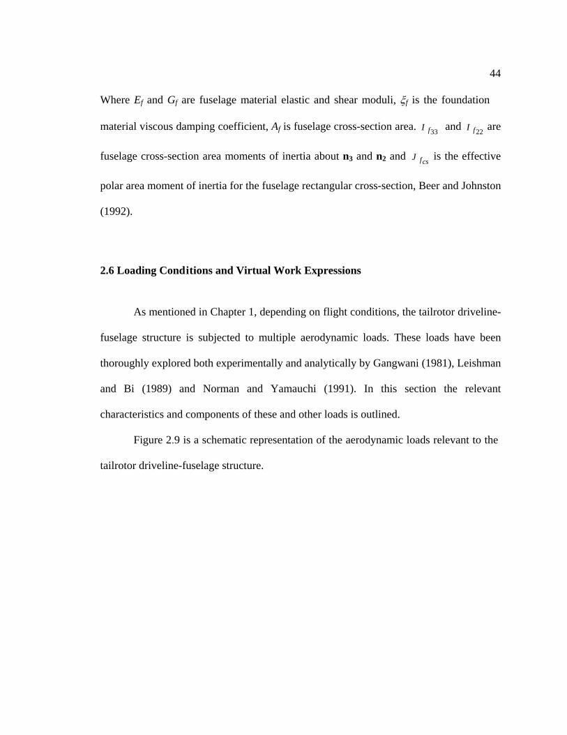
44

Where Ef and Gf are fuselage material elastic and shear moduli, ξf is the foundation

material viscous damping coefficient, Af is fuselage cross-section area. 33fI and 22fI are

fuselage cross-section area moments of inertia about n3 and n2 and csfJ is the effective

polar area moment of inertia for the fuselage rectangular cross-section, Beer and Johnston

(1992).

2.6 Loading Conditions and Virtual Work Expressions

As mentioned in Chapter 1, depending on flight conditions, the tailrotor driveline-

fuselage structure is subjected to multiple aerodynamic loads. These loads have been

thoroughly explored both experimentally and analytically by Gangwani (1981), Leishman

and Bi (1989) and Norman and Yamauchi (1991). In this section the relevant

characteristics and components of these and other loads is outlined.

Figure 2.9 is a schematic representation of the aerodynamic loads relevant to the

tailrotor driveline-fuselage structure.

45

The horizontal-stabilizer lift and drag forces are LiftF and DragF , and the horizontal-

stabilizer pitch and roll moments are PitchM and RollM . For a helicopter in forward flight,

the steady part of these forces and moments are due to standard airfoil lift and drag

effects. Following Gangwani (1981), these forces and moments are described by,

chsFairRRollchsFairPPitch

hsFairDDraghsFairLLift

LAVCtMLAVCtM

AVCtFAVCtF2

212

21

2212

21

)( ,)(

)( ,)(

ρρ

ρρ

==

==(2.37)

Where LC , DC , PC , and RC are the lift, drag, pitch and roll coefficients, ρair is air-

density, VF is helicopter forward speed, and Ahs and Lc are the horizontal stabilizer

surface area and chord length. According to Leishman and Bi (1989), in hover and in

forward flight, another major source of steady loading on the tailboom structure is main-

rotor downwash. The downwash loads, SWf and DWf , act in both the horizontal and

vertical directions and are distributed along the length of tailboom. These loads are

described as

E

Fuselage Beam

Tailrotor Hub

H

O

n1n3

n2

2TRd

1TRd

DragF

LiftF

RollMPitchM

TRF

SWf

DWf

Fig. 2.9: Aerodynamic loads on tailrotor driveline-fuselage structure.

46

sidetipairsidepSWtoptipairtoppDW WVCxfWVCxf 2212

21 )( ,-)( ρρ == (2.38)

Where )(xC topp and )(xC sidep are distributed pressure coefficients along the top and sides

of the tailboom beam, Wtop(x) and Wside(x) are the planform widths of the tailboom top

and side, and Vtip is main-rotor tip speed. Both Leishman and Bi (1989) and Norman and

Yamauchi (1991) measured these pressure coefficients on scaled helicopter models in

wind tunnel experiments where is was shown that the pressure coefficients, PtopC and

PsideC , mainly depend on axial location, x, blade-loading coefficient CT/δ, forward speed

advance ratio µ, and the main-rotor tilt angle, αs. Finally, another significant source of

steady aerodynamic loading is the tail-rotor anti-torque force, FTR , which counteracts the

main-rotor torque TMR.

HLMRT

TRF = (2.39)

Here, LH is the distance from the main-rotor hub to the tail-rotor hub. The virtual work

expressions for the above aerodynamic loads are written as

[ ]

TRTBHSaero

TRffTRffffTRTR

fLfSWfDWTB

ffPitchffRollffDragffLiftHS

WWWW

dtLdtLwtLwFW

dxtxwxftxvxfW

tLvMtLMtLuFtLvFW

δδδδ

φδδ

δδδ

δφδδδδ

++=

+′+=

+=

′+++=

∫]),(ˆ),(),([

)],([)()],([)(-

)],([)],(ˆ[)],([)],([

21

0 (2.40)

Another significant excitation source inherent to all drivelines is rotational

imbalance. Rotation imbalance occurs when the mass center of the shaft cross-section is

not coincident with the rotation axis. This is due to density variations and shaft geometric

47

imperfections that act like distributed mass imbalance, iimbm , at radial and angular

locations, iimbr and i

imbφ , on the shaft cross-section.

The distributed imbalance force, iimbfr

, is given as

20

20 )()()( and

)](sin[)(),(

)](cos[)(),(

with

),(),(),(

Ω=Ω=

+=

+=

+=

sicciimb

iimb

iimb

iimbi

iimb

iimbw

iimbi

iimb

iimbv

iimbw

iimbv

iimb

mxexrxmfxxftxf

xxftxf

txftxftxf

φφ

φφ

i3

i2 mm

v

(2.41)

For an initially bent shaft, with deformed shape )(xv roi and )(xw roi , the imbalance

parameters are given by

=+== −

)(

)(tan)( ,)()()( ,)( 122

xv

xwxxwxvxrmxm

iro

iroiimbiroiro

iimbs

iimb φ (2.42)

Since imbalance is typically specified by eccentricity, the following cross-sectional shaft

eccentricity, icce , is defined as (2.43).

i3m

i3r

i2r

i2m

iφ

iimbφ

iimbr

iimbm

iimbfv

Ds

ts

Fig. 2.10: Cross-section of ith shaft with mass imbalance.

48

+= i

imbs

iimbi

imbiccmm

mre

(2.43)

Which the measures cross-sectional mass center offset from the shaft geometric center.

The virtual work expression for the shaft rotational imbalance force is

∑∫=

+=

2

10

)],([),()],([),(i

iLi

iimbwi

iimbvimb dxtxwtxftxvtxfW δδδ (2.44)

To account for axial loading of the driveline, the virtual work expression for the

static axial load, Pa, is given as

[ ]22

2

10 Lxa

i

iLiiiiaaP uPdxwwvvPW =

=

−′′+′′= ∑∫ δδδδ (2.45)

Furthermore, to account for the tail-rotor torque-load, the virtual work expression for the

resistive torque-load, TL, is given by

[ ] LLi

iLiiiiLLT TdxvwwvTW δφδδδ −′′′−′′′= ∑∫

=

2

10

(2.46)

Here TL is the effective torque-load as seen through the intermediate gearbox. The first

term of this expression accounts for the so-called axial torque effect on the intermediate

roiv

xi3r i

1r

i2r

roiw

Fig. 2.11: Shaft geometric imperfection: initially bent shaft.

49

shafts, derived in Zorzi and Nelson (1979), and the second term accounts for the

torque load on the output-shaft.

Finally, to account for effects of gravity, g, in the n1-n2 plane, (2.47) gives the

virtual work expression for the gravity loading.

[ ]∑∫ ∫=

−−=

2

10 0

)],([ )],([i

iL fLffisgrav dxtxvgmdxtxvgmW δδδ (2.47)

2.7 Finite Elemen t Formulation and Equations-of-Motion

In this section, the finite-element-method together with Lagrange’s equations are

employed to obtain equations-of-motion for the tailrotor driveline-fuselage structure. The

two intermediate shafts, (i = 1, 2), and the fuselage beam, (i = f), are discreteized into ielN

two-node beam-rod-torsion elements each with element length ieli

iel NLL /= . Figure 2.12

shows the jth element of the ith structure with two 6-degree-of-freedom (DOF) nodes.

Equation (2.48) shows the corresponding nodal and elemental displacement vectors

==

+i

jnode

ijnodei

jelT

jijijijijijii

jnode q

qquwvq

1,

,,,1,,2,,3,, and ][ θθθ (2.48)

Finally, the number of nodes in the ith assembled structure is related to the number of

elements by

NN iel

inode 1 += (2.49)

50

The displacements on the domain of the ith structure at the jth element are related to the

elemental displacement vector, ijelq , by

)( ),(),(ˆ ),( ),(),(

)( ),(),( ),( ),(),(

)( ),(),( ),( ),(),(

tqLxNtxtqLxNtxu

tqLxNtxwtqLxNtxv

tqLxNtxwtqLxNtxv

ijel

ieleli

ijel

ielelui

ijel

ielelwi

ijel

ielelvi

ijel

ielelwi

ijel

ielelvi

φφ ==

′=′′=′

==

(2.50)

where ielel Ljxx )1( −−= , and with shape functions Nv, Nw, Nu and Nφ defined as

−=

−=

−−−+−+−=

−−+−+−=

elLelx

elLelx

elLelx

elLelx

u

elLelx

elLelx

elLelx

elLelx

elLelx

elLelx

elelLelx

elLelx

w

elLelx

elLelx

elLelx

elLelx

elLelx

elLelx

elelLelx

elLelx

v

NN

xN

xN

0, ,0 ,0 ,0 ,0 ,0,1 ,0 ,0 ,0 ,0 ,0 , ,0 ,0 ,0 ,0 ,1 ,0 ,0 ,0 ,0

0 ,0 ,,23 ,0 ,0 ,0 ,0 ,2 ,231 ,0 ,0

0 ,0 ,0 ,0 , ,23 ,0 ,0 ,0 ,0 ,2 ,231

2

32

3

3

2

2

2

32

3

3

2

2

2

2

3

3

3

2

2

2

32

3

3

2

2

φ

(2.51)

Here Nv, and Nw are based on cubic polynomial interpolation functions and Nu and Nφ are

based on linear interpolation functions, Meirovitch, (1980). After substituting the

displacements in Equation (2.50) into the previously derived energy, dissipation and

virtual work expressions and defining the global displacement vector, 1×ℜ∈ dofNq , as

j1+j

jiv ,

ji,3θ

jiw , ji,2θ

jiu ,

ji,1θ

1, +jiw 1,2 +jiθ1,1 +jiθ

1, +jiu

1,3 +jiθ

1, +jivielL

elx

NodeNode

Fig. 2.12: jth beam-rod-torsion finite element of the ith structure.

51

,1,

22,

21,

11,

11,

TTf

fnodeNnode

Tfnode

T

nodeNnode

Tnode

T

nodeNnode

Tnode qqqqqqq

= LLL (2.52)

the unconstrained equations-of-motions, are obtained using Lagrange’s Equations as

gravaeroimbLTaPdbcsf

bcsfLJstfLJstf

QQQQQq

DDDDD

qVVVV

qTTTT

qTTTT

dtd

++++=∂

++++∂+

∂

+++∂+

∂

+++∂−

∂

+++∂

&L

&

)(

)()()(

(2.53)

The undamped gyroscopic portion of the system with zero load-torque, zero axial-load,

zero static misalignment and no external loading or excitation is

qqqq

VVVVq

TTTq

TTTdtd bcsfstfstf KGM +Ω+≡

∂

+++∂+

∂

++∂−

∂

++∂&&&

&)(

)()()(0 (2.54)

Here M, G, and K are the nominal mass, gyroscopic, and elastic stiffness matrices. See

Appendix A for the elemental matrices. Since output-shaft speed, LΩ , is a function of the

input-shaft speed, 0Ω , the static misalignments, δ2, δ3, ξ2, ξ3, γ2, γ3, and the dynamic

misalignments, which are functions of q and q& , the inertia-load terms are,

)1()()()()( 6−∆∆∆∆ +−++≡

∂Ω∂

−

∂Ω∂

Ω+∂Ω∂

Ω=∂

∂−

∂

∂

eOtqtqtqt

qqdtdJ

qJ

qT

qT

dtd LL

LLL

LLLJLJ

FKCM &&&

&&&

& (2.55)

Here the linear inertia-load terms are composed of the periodic inertia, damping, stiffness

and forcing terms, corresponding to )()( pTtt += ∆∆ MM , )()( pTtt += ∆∆ CC , )()( pTtt += ∆∆ KK

and )()( pTtt += ∆∆ FF respectively with period 0Ω=π

pT . These periodic coupling matrices

and forcing terms are functions of the static misalignment angles, input shaft speed, and

inertia-load, JL. See Appendix B.

The dissipation terms of the system are

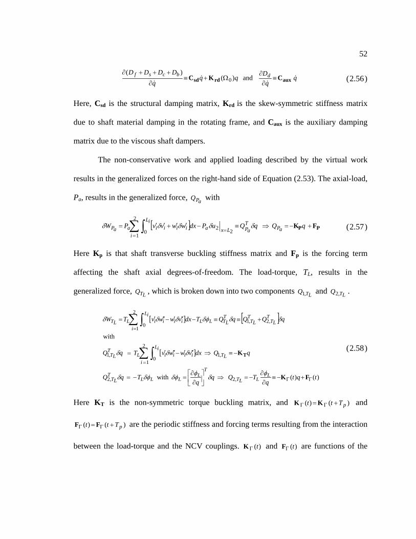
52

qq

Dqq

qDDDD dbcsf

&&

&&

and )()(

0 auxrdsd CKC ≡∂∂

Ω+≡∂

+++∂(2.56)

Here, Csd is the structural damping matrix, Krd is the skew-symmetric stiffness matrix

due to shaft material damping in the rotating frame, and Caux is the auxiliary damping

matrix due to the viscous shaft dampers.

The non-conservative work and applied loading described by the virtual work

results in the generalized forces on the right-hand side of Equation (2.53). The axial-load,

Pa, results in the generalized force, aPQ with

[ ] PP FK +−=⇒≡−′′+′′==

=∑∫ qQqQuPdxwwvvPW aP

TaPLxa

i

iLiiiiaaP

22

2

10

δδδδδ (2.57)

Here Kp is that shaft transverse buckling stiffness matrix and Fp is the forcing term

affecting the shaft axial degrees-of-freedom. The load-torque, TL, results in the

generalized force, LTQ , which is broken down into two components LTQ ,1 and LTQ ,2 .

[ ] [ ]

[ ]

)()( with

with

,2,2

,1

2

10

,1

,2,1

2

10

tqtq

TQqq

TqQ

qQdxvwwvTqQ

qQQqQTdxvwwvTW

LLLT

TL

LLLT

LT

LTi

iLiiiiL

TLT

TLT

TLT

TLTLL

i

iLiiiiLLT

ΓΓ

=

=

+−≡∂∂

−=⇒

∂∂

=−=

−≡⇒′′′−′′′=

+≡≡−′′′−′′′=

∑∫

∑∫

FK

KT

φδφδφδφδ

δδδ

δδδφδδδ

(2.58)

Here KT is the non-symmetric torque buckling matrix, and )()( pTtt += ΓΓ KK and

)()( pTtt += ΓΓ FF are the periodic stiffness and forcing terms resulting from the interaction

between the load-torque and the NCV couplings. )(tΓK and )(tΓF are functions of the

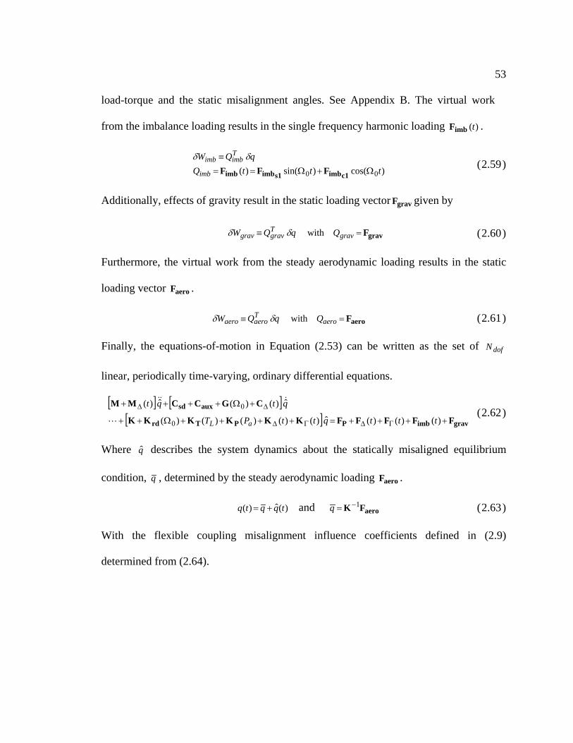
53

load-torque and the static misalignment angles. See Appendix B. The virtual work

from the imbalance loading results in the single frequency harmonic loading )(timbF .

)cos()sin()(

00 tttQqQW

imb

Timbimb

Ω+Ω==≡

c1imbs1imbimb FFFδδ

(2.59)

Additionally, effects of gravity result in the static loading vector gravF given by

gravF=≡ gravTgravgrav QqQW with δδ (2.60)

Furthermore, the virtual work from the steady aerodynamic loading results in the static

loading vector aeroF .

aeroF=≡ aeroTaeroaero QqQW with δδ (2.61)

Finally, the equations-of-motion in Equation (2.53) can be written as the set of dofN

linear, periodically time-varying, ordinary differential equations.

[ ] [ ][ ] gravimbPPTrd

auxsd

FFFFFKKKKKK

CGCCMM

++++=++++Ω++

+Ω++++

Γ∆Γ∆

∆∆

)()()(ˆ )()()()()(

ˆ )()(ˆ )(

0

0

tttqttPT

qtqt

aLL

&&&

(2.62)

Where q describes the system dynamics about the statically misaligned equilibrium

condition, q , determined by the steady aerodynamic loading aeroF .

)(ˆ)( tqqtq += and aeroFK 1 −=q (2.63)

With the flexible coupling misalignment influence coefficients defined in (2.9)

determined from (2.64).

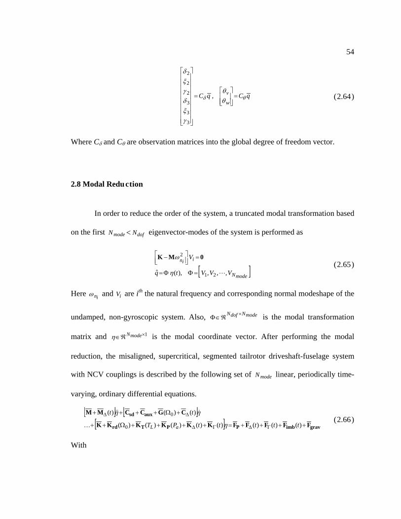
54

qCqCw

vθδ θ

θ

γξδγξδ

=

=

,

3

3

3

2

2

2

(2.64)

Where Cδ and Cθ are observation matrices into the global degree of freedom vector.

2.8 Modal Reduction

In order to reduce the order of the system, a truncated modal transformation based

on the first modeN < dofN eigenvector-modes of the system is performed as

[ ]modeN

iin

VVVtq

V

, , , ),( ˆ

21

2

L=ΦΦ=

=

−

η

ω 0MK(2.65)

Here inω and iV are ith the natural frequency and corresponding normal modeshape of the

undamped, non-gyroscopic system. Also, modeNdofN ×ℜ∈Φ is the modal transformation

matrix and 1 ×ℜ∈ modeNη is the modal coordinate vector. After performing the modal

reduction, the misaligned, supercritical, segmented tailrotor driveshaft-fuselage system

with NCV couplings is described by the following set of modeN linear, periodically time-

varying, ordinary differential equations.

[ ] [ ][ ] gravimbPPTrd

auxsd

FFFFFKKKKKK

CGCCMM

++++=++++Ω++

+Ω++++

Γ∆Γ∆

∆∆

)()()()()()()()(

)()()(

0

0

tttttPT

tt

aL η

ηη

K

&&&(2.66)

With

55

gravgravimbimbPP

PP

TTrdrd

auxauxsdsd

FFFFFFFFFF

KKKKKK

KKKKKK

CCGG

CCCC

MMMIM

TTTTT

TTT

TTT

TT

TT

TT

tttttt

tttt

tt

tt

Φ=Φ=Φ=Φ=Φ=

ΦΦ=ΦΦ=ΦΦ=

ΦΦ=ΦΦ=ΦΦ=

ΦΦ=ΦΦ=

ΦΦ=ΦΦ=

ΦΦ=ΦΦ==

ΓΓ∆∆

ΓΓ∆∆

∆∆

∆∆

),()( ),()( ),()( ,

)()( ,)()( ,

, ,

)()( ,

, ,

)()( ,

(2.67)

2.9 Magnetic Bearings

In this section, the force-current-displacement relations are derived for the

magnetic bearings discussed in Section 1.5. Figure 2.13 is a cross-section of an 8-pole

radial Active Magnetic Bearing (AMB). Here, the coils in each quadrant I, II, III, and IV

are wired in series and have currents Icoili , IIcoili , IIIcoili and IVcoili .

IcoiliS S

N

N N

SS

N

gaphi3m

bv ,2b

i2m

bθ

C

bw ,3b

I

II III

IV

IIcoili

IIIcoili

IVcoili

3bF

2bF

Fig. 2.13: 8-pole radial AMB with bias and control currents.

56

To produce the net actuation force, 2bF , in the b2 direction, quadrants I and III are

operated together and, likewise, quadrants II and IV operate together to generate the

actuation force 3bF , in the b3 direction. In particular, the coil currents are operated about

a bias current level, ibias, and the coil currents are given as

3IV3II

2III2I

,

,

iiiiii

iiiiii

biascoilbiascoil

biascoilbiascoil

−=+=

−=+=(2.68)

Here i2 and i3 are the AMB control currents. Based on the force-current-displacement

relation for an individual coil, (1.2), the net actuation forces are

+−

−−+

= 2

22

2

22

2 )()(

)()(

bgap

bias

bgap

biasbb vh

iivhiiGF and

+−

−−+

= 2

23

2

23

3 )()(

)()(

bgap

bias

bgap

biasbb wh

iiwhiiGF (2.69)

Where vb and wb are the shaft displacements relative to the AMB stator and hgap is the

nominal rotor-stator airgap distance. Also, the AMB force constant Gb is

( ) 208cos wpb NAG µπ≡ (2.70)

Where µ0 is the magnetic permeability of free-space, Ap is the pole face area and Nw is the

number of coil windings. After linearizing about the bias current and the nominal airgap,

the linearized force-current-displacement relations for the kth AMB become

+

=

k

k

i

i

kb

kb

x

x

kb

kbii

kk

wv

kk

FF

,3

,2

,

,

,3

,20

00

0(2.71)

with the AMB force-position and force-current gains, kx and ki given as

3

24

gap

biasbx

h

iGk = and 2

4

gap

biasbi

hiG

k = (2.72)

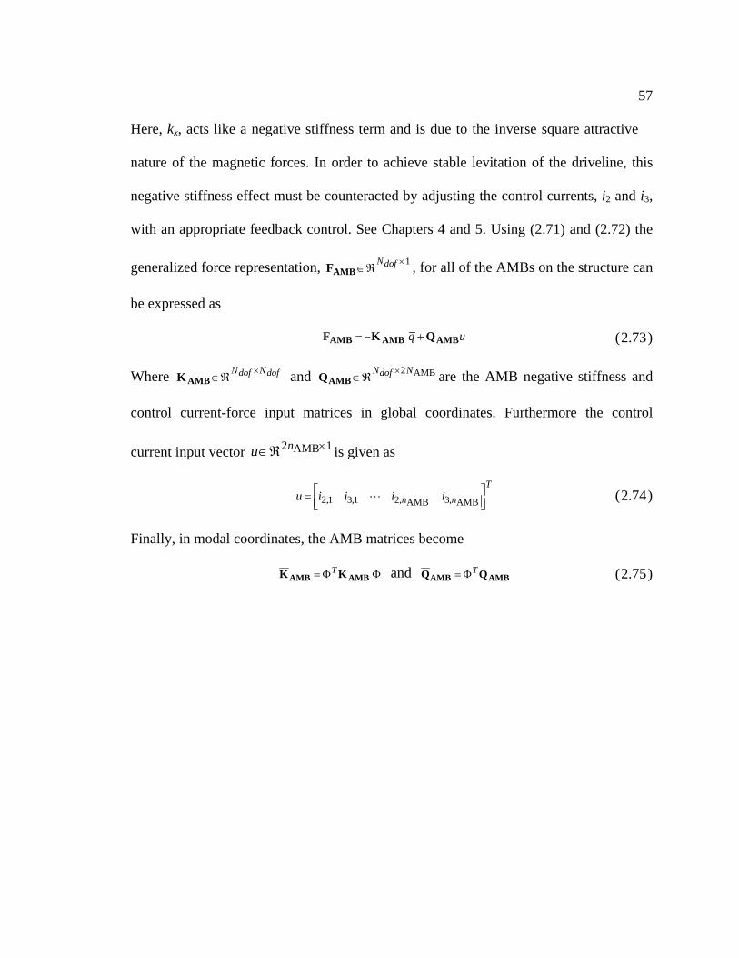
57

Here, kx, acts like a negative stiffness term and is due to the inverse square attractive

nature of the magnetic forces. In order to achieve stable levitation of the driveline, this

negative stiffness effect must be counteracted by adjusting the control currents, i2 and i3,

with an appropriate feedback control. See Chapters 4 and 5. Using (2.71) and (2.72) the

generalized force representation, 1 ×ℜ∈ dofN

AMBF , for all of the AMBs on the structure can

be expressed as

uq AMBAMBAMB QKF +−= (2.73)

Where dofNdofN ×ℜ∈AMBK and AMB2NdofN ×

ℜ∈AMBQ are the AMB negative stiffness and

control current-force input matrices in global coordinates. Furthermore the control

current input vector 1 AMB2 ×ℜ∈ nu is given as

Tnn iiiiu

= AMB,3AMB,21,31,2 L (2.74)

Finally, in modal coordinates, the AMB matrices become

ΦΦ= AMBAMB KK T and AMBAMB QQ TΦ= (2.75)

58

Chapter 3

STABILITY ANALYSIS OF A SEGMENTED SUPERCRITICAL DRIVELINE

WITH NCV COUPLINGS SUBJECT TO MISALIGNMENT AND TORQUE

3.1 Introduction

To gain insight and develop design guidelines for the Configuration I active

vibration control, a non-dimensional stability analysis of a conventional segmented

driveline is performed. As discussed in Chapter 1, many researchers have studied the

stability of shafts operating at supercritical speeds, where it has been shown that internal

(rotating-frame) damping tends to cause whirl instability depending on the amount of

external (fixed-frame) damping present. However, the effect of non-constant velocity

(NCV) couplings has not been included in these analyses. Some researchers explored the

stability of single U-joint/shaft-disk systems, where it has been shown that misalignment

and load-torque generate periodic parametric terms that cause instability near certain

shaft speeds. While the results were interesting, the single U-joint system does not really

resemble a typical driveline. Furthermore, previous analyses of double U-joint/shaft

systems only considered the periodic moment forcing terms, but neglected the potentially

59

destabilizing periodic parametric terms. Hence, the stability behavior of a segmented

driveline involving multiple NCV couplings has not been studied. Since most drivelines

consist of two or more flexible couplings, depending on the number of segments, it is

important to understand the effect of misalignment and load-torque on the stability of

such multi-coupling/shaft systems. Furthermore, with the trend toward supercritical

drivelines, the interaction between different instability regions due to misalignment, load-

torque and the rotating-frame damping-induced whirl instability must be assessed.

3.2 Driveline Non-Dimensional Equations-of-Motion

Equations of motion are derived for the segmented driveline system shown in

Figure 3.1. This is very similar to the conventional tailrotor driveline system discussed in

Chapter 2; however, to reduce complexity and obtain a non-dimensional formulation, the

driveline is assumed to be mounted on a rigid foundation with a rigid hanger-bearing.

Neglecting fuselage flexibility is a mild assumption since the fuselage structure is

typically much larger and stiffer than the driveline. Also, the couplings are assumed to be

rigid in the transverse direction, thus giving the intermediate shafts pinned-pinned

boundary conditions in transverse directions. Furthermore, the static misalignment

configuration considered in this chapter is less general in Chapter 2. The system consists

of a fixed input-shaft, a fixed output-shaft, and two flexible intermediate shafts with

lengths L. The shafts are connected by U-joint couplings A, B and C that are nominally

phased by 90°, as is typically the case, Mancuso (1986). Specifically, the U-joint phase

angles are, ψA = 0°, ψB = 90° and ψC = 0°. The intermediate shafts are flexible in bending

60

and torsion and are supported on a rigid bearing. The two mid-span dampers, with

damping coefficient Cd, provide auxiliary viscous lateral damping to counteract

destabilizing effects of shaft internal damping.

Here m=[m1, m2, m3], a fixed-frame aligned with intermediate shafts with m3 normal

to the page. The transverse displacements measured from the m frame are defined as

≤≤−≤≤=

≤≤−≤≤= LxLtLxw

LxtxwtxwLxLtLxvLxtxvtxv 2 ),(

0 ),(),( , 2 ),(0 ),(),(

21

21 ( 3.1 )

Where ),( txv and ),( txw measure deflection in the m2 and m3 directions. The total shaft

rotation angle, ),( txφ , and elastic windup angle, ),( txφ , are defined as

≤≤−≤≤=

≤≤−+=−≤≤+==

LxLtLxLxtxtx

LxLtLxttLxLxtxttxtx

2 ),(0 ),(

),( , 2 ),( )( ),(

0 ),( )( ),(),(2

1

222

111φφφ

φφφφφφφ ( 3.2 )

where )(tiφ are rigid body rotations and ),( txiφ are elastic twist deformations of the

intermediate shafts. It is assumed that input-shaft is driven at a constant speed, 0Ω , and

the output-shaft drives both a torsional inertial-load, JL, and a resistive torque-load, TL,

with rotational speed )(tLΩ . Furthermore, the driveline is subjected to the static

Inertia-Load, JL

Torque-Load, TL

δ

γ

B

C

Damper

RigidBearing

U-Joint

L

L

Cd

Cd

A

ψA

ψC

ψB OutputShaft

InputShaft

),(),(

22

22

txwtxv

),(),(

11

11

txwtxv

),( 11 txφ

),( 22 txφ

)( ),( tt LL Ωφ

tt 00 )( Ω=φ

Damper11 m

12 m

22 m

21 m

0=x

m2

m1

m3

Fig. 3.1: Segmented driveline connected by U-joint couplings.

61

misalignments, δ and γ, at the input-shaft and output-shafts in the m1-m2 plane. In terms

of the driveline static misalignments defined in Chapter 2, the misalignment angles for

this configuration are [δ2 = δ, δ3 = 0, ξ2 = 0, ξ3 = 0, γ2 = γ, γ3 = 0]. Substituting these

misalignments into Equation (2.11) gives the output-shaft rotation angle, )(tLφ , as

( ) ( )

′−−′+′−′−+

′−′+′′−−′′+−

′−−′−−′−′−

′−′−−′′−′+−′+

′′+′−′+′+′′−′′+′++=

))(()()21()2cos(

)()21()()2cos(

))()(21()(4)2sin(

))(21(4)()2sin(

) ( )(

2,2

2,2,2,2,2

2,202

1

22,1

2,1,1,102

1

2,2

2,2

2,2,2,2,204

1

222,1,1

2,1

2,104

1

,2,282

,2,1,2,2,1,121

0,2

CCCCCC

BBBBBBAA

CCCCCC

BBBBBBAA

BBCCCBBBBACL

wvwv

wvwvvw

wvwv

wvwvwv

wvwvvwvwvvt

γφγφφ

φφδφ

γφγφφ

φφδφ

γγδφφφ δ

L

L

L

L

( 3.3 )

With the small dynamic misalignments due to the elastic slopes of the intermediate shafts

at the couplings defined as

LxCLxC

xBxB

LxBLxB

xAxA

txwtwtxvtv

txwtwtxvtv

txwtwtxvtv

txwtwtxvtv

==

==

==

==

′=′′=′

′=′′=′

′=′′=′

′=′′=′

),()( ,),()(

),()( ,),()(

),()( ,),()(

),()( ,),()(

2,22,2

02,202,2

1,11,1

01,101,1

and )()()(

)()()(

,1,2

,1,2

twtwtw

tvtvtv

BBB

BBB

′−′=′

′−′=′( 3.4 )

and the shaft elastic windup angles at the couplings B and C defined as

LxsCC

LxsBB txttxt

==+=+= ),()( and ),()(

2,21,1 φφφφφφ ( 3.5 )

Where sBφ and sCφ are the static portions of the elastic windup due to the load torque,

TL, which are

ss

LsBsC

ss

LsB JG

LTJGLT

+== φφφ and ( 3.6 )

Furthermore, the time derivative of (3.3) yields the output-shaft speed, )()( tt LL φ&=Ω .

The total kinetic energy of the driveline is

62

22

022222

2 ])[ (

2)(

2)(

2 LL

Lsss Jdxwvvw

Jmwv

Imwv

mT Ω+

′′−′′Ω+Ω+′+′++= ∫ &&&&&& ( 3.7 )

Since it is assumed that Ls JLJm << , the effect of the intermediate shaft speed variation

on the equations-of-motion is negligible compared to the effect of the output-shaft speed

variation. Hence the full expressions for Lφ and LΩ are used in the derivation but φ and

Ω are approximated as

),(),( and ),(),( 00 txtxtxttx φφφ &+Ω≈Ω+Ω≈ ( 3.8 )

The total driveline strain energy is

dxJG

wvIE

VL

ssss 2

)(2

2

0222∫

′+′′+′′= φ ( 3.9 )

The total driveline Rayleigh dissipation function is 3.10

2

22

2

22

2

02222

0022

22

2

][][22

LLx

dLx

d

Lssss

s

wvC

wvC

dxJG

wvvwwvwvIE

D

+==

++

++

′+

′′+′′Ω+′′′′−′′′′Ω+′′+′′= ∫

&&&&L

&&&&& φξ

(3.10)

Here D accounts for both the rotating-frame shaft viscous material damping and the

fixed-frame auxiliary dampers with damping coefficient Cd.

To obtain equations-of-motion, the shaft transverse deflections, ),( txv and

),( txw , and the shaft elastic twist angle, ),( txφ , are written in terms of the following

modal expansion,

)()(),( ),()(),( ),()( ),( txtxtxtxwtxtxv wv ηφηη φΦ=Φ=Φ= (3.11)

Where )(tη is the n ×1 column vector of modal coordinates and xv )(Φ , xw )(Φ and

x)(Φφ are the corresponding row vectors of assumed mode shapes.

63

LxLxx

LxLLLx

LxLLxx

LxLLLx

LxLLxx

LLx

LLx

w

Lx

Lx

ww

LLx

LLx

v

Lx

Lx

vv

20 2

00000000)(

2 ]0sin000sin000[)(

0 ]000sin000sin0[)()(

2 ]00sin000sin00[)(

0 ]0000sin000sin[)()(

)(2)(2

21

)(2)(2

21

≤≤

=Φ

≤≤=Φ

≤≤=Φ=Φ

≤≤=Φ

≤≤=Φ=Φ

−−

−−

φ

ππ

ππ

ππ

ππ

(3.12)

Here xv )(Φ and xw )(Φ contain the first two pinned-pinned bending mode shapes for

both intermediate shafts, and x)(Φφ is composed of the first fixed-free twisting mode

shape. After substitution of the modal expansions (3.11) and (3.12), the functional

representation of the output-shaft speed and rotation angle becomes

),,,,( 0 ηγδφφ Ω= tLL and ),,,,,( 0 ηηγδ &ΩΩ=Ω tLL (3.13)

The virtual work, W LTδ , and corresponding generalized force vector, Q LT , due to the

output-shaft resistive torque load, TL, are

ηφ

δηη

φδφδηδφδ

∂∂

−=

∂

∂=≡−= L

LLT

TL

LTLTLLLT TQQTW thus with , (3.14)

After substituting the modal expansions into the energy and dissipation expressions in

(3.7), (3.9) and (3.10), the equations-of-motion obtained via Lagranges equations are

[ ] [ ] 0 =∂

∂+

∂Ω∂

−

∂Ω∂

Ω+∂Ω∂

Ω++++++

=−∂∂

+∂∂

+∂∂

−

∂∂

ηφ

ηηηηηη

ηηηη

LL

LLLL

LLL

LT

TdtdJJ

QDVTTdtd

&&&&&&

&&

rdauxsd KKCCGM

Nominal System Misalignment & Torque NCV Terms

(3.15)

Where the nominal system matrices are

64

∫∫

∫∫

∫

Φ ′′Φ ′′−Φ ′′Φ ′′Ω=

Φ′Φ′+

Φ ′′Φ ′′+Φ ′′Φ ′′=

ΦΦ+ΦΦ+

ΦΦ+ΦΦ=

Φ′Φ′+

Φ ′′Φ ′′+Φ ′′Φ ′′=

Φ′Φ′−Φ′Φ′Ω=

ΦΦ+

Φ′Φ′+Φ′Φ′+

ΦΦ+ΦΦ=

==

Lv

Tww

Tvsss

L Tssw

Twv

Tvss

Lxw

Twv

TvLx

wTwv

Tvd

L Tssw

Twv

Tvsss

Lv

Tww

Tvs

L Tsw

Twv

Tvsw

Twv

Tvs

dxIE

dxJGIE

c

dxJGIE

dxJm

dxJmImm

2

00

2

0

23

2

2

0

2

00

2

0

ξ

ξ

φφ

φφ

φφ

rd

aux

sd

K

K

C

C

G

M

(3.16)

M, G, and K are shaft inertia, gyroscopic and elastic stiffness matrices, Csd and Caux are

the shaft structural and auxiliary damping matrices, and Krd is the skew-symmetric

stiffness matrix due to the rotating-frame damping. The NCV terms due to misalignment

and load-torque are obtained by substituting the expressions for Lφ and LΩ into (3.15)

and taking the necessary partial and time derivatives. After this procedure it becomes

apparent that

0=∂Ω∂

−

∂Ω∂

ηηLL

dtd

&(3.17)

After dropping higher-order non-linear terms, the terms due to misalignment become

[ ]

[ ][ ][ ])2cos()2sin(

)2cos()2sin(

)2cos()2sin(

)2cos()2sin(

02020

02020

02020

02020

tt

tt

tt

ttJ

cs

cs

cs

csL

LL

Ω+Ω+−

Ω+Ω++

Ω+Ω++

Ω+Ω+=∂Ω∂

Ω

∆∆∆

∆∆∆

∆∆∆

∆∆∆

FFF

KKK

CCC

MMM

L

L

&L

&&&

&

η

η

ηη

(3.18)

and the terms due to load-torque become

65

[ ]

[ ])2cos()2sin(

)2cos()2sin(

02020

02020

tt

ttT

cs

csL

L

Ω+Ω+−

Ω+Ω+=∂

∂

ΓΓΓ

ΓΓΓ

FFF

KKK

L

ηη

φ

(3.19)

After substituting (3.17), (3.18) and (3.19) into (3.15), the equations-of-motion become a

set of n second-order linear periodically time-varying equations, see Equation (3.20).

[ ][ ]

( ) ( )[ ]( ) ( ) )2sin()2cos(

)2sin()2cos(

)2sin()2cos(

)2sin()2cos(

02202200

02202200

*02020

* *02020

tftf

tftf

tftf

tftf

sscc

sscc

sc

sc

Γ∆Γ∆Γ∆

Γ∆Γ∆Γ∆

∆∆∆

∆∆∆

+++++=

++++++++

++++++

+++

FFFFFF

KKKKKKKK

CCCCCG

MMMM

rd

auxsd

L

L

L

η

η

η

(3.20)

and the nominal equations-of-motion are

[ ] [ ] 0KKCCGM rdauxsd =+++++ ηηη ** * (3.21)

Here the equations have been non-dimensionalized with respect to the first pinned-pinned

bending natural frequency, NDΩ , and the intermediate shaft segment length, L. The *

operator indicates differentiation with respect to non-dimensional (N.D.) time, t . The

relevant N.D. parameters for a solid circular cross-section shaft are shown in Equations

(3.22) (3.25).

Ld

Lww

Lvv

Lxxtt

LmIE

NDs

ssND ====Ω==Ω ε

π , , , , ,4

4(3.22)

Where the N.D. shaft displacements are v , w and the N.D. axial coordinates is x . Also,

the shaft slenderness ratio based on shaft diameter, d, is ε.

φφ

τφφυπυεπ

εττµ

kk

LmT

LmJ

sCsshear

NDs

L

s

L −==+

=+

=Ω

== ,)1(2

1 ,)1(

2 , , 44max233 (3.23)

Also, µ and τ are the N.D. load-inertia and load-torque parameters and τmax is the

maximum load-torque parameter based on the material shear yield strain, εshear, and

66

Poissons ratio, υ. The N.D. torsion stiffness is, kφ, and the static windup angle of the

driveline at coupling C due to τ, is φs.

µεµ

φφφ

πεπε

kkffff

ND≈

+

=≈+

=≈+

=ΩΩ

=

)12

( ,4

1

14 ,11

1 , 24

222

16221

00 (3.24)

The N.D. input-shaft speed is f0, the first two N.D. bending natural frequencies are f1 and

f2, and the first N.D. torsion natural frequency is fφ.

NDs

dd

NDsNDsNDsLmC

cfff Ω

=Ω

=Ω

=Ω

= ,2

,2

,2 2

21

1φ

φξ

ζξ

ζξ

ζ (3.25)

Furthermore, ζ1, ζ2 and ζφ are the modal damping ratios and cd is the N.D. auxiliary

damping coefficient. Finally, the driveline equations-of-motion in (3.20) are valid under

the parameter constraints shown in (3.26).

max2 , )1(5

32 ,1 ττυεπ

ε φ <+

<<⇒<<<< fJLJm Ls (3.26)

The N.D. nominal system matrices are KCCGM auxsd , , , , and sdK , and the remaining

matrices and forcing terms are the NCV terms due to misalignment and load-torque. The

inertia matrices, 220 and , cs ∆∆∆ MMM , the damping matrices, 220 and , cs ∆∆∆ CCC , the

stiffness matrices, 220 and , cs ∆∆∆ KKK , and forcing terms, 220 and , cs ∆∆∆ FFF , are

functions of the static misalignment angles, δ and γ, the inertia-load parameter, µ, and the

static windup angle φs. Furthermore, the stiffness matrices, 220 and , cs ΓΓΓ KKK , and

forcing terms, 220 and , cs ΓΓΓ FFF , are functions of the load-torque parameter, τ, and the

static windup angle φs.

67

3.3 Stability Analysis

In the following sub-sections, the stability behavior of Equations (3.20) and (3.21)

is analyzed. To establish a baseline for studying the stability of the full system, (3.20), the

effect of shaft internal and external damping on the stability of the nominal system,

(3.21), is first examined. Next, the stability of the full system is explored including the

effects of internal and external damping, driveline misalignment, and load-torque.

As a basis for analysis, the parameters for a typical rotorcraft supercritical

driveline are used in the equations. The shaft slenderness ratio is ε = 0.012, the modal

damping ratios are ζ1 = ζ2 = ζφ = ζ = 0.002, the shaft material shear yield strain is ε shear =

2.7x10-3, and Poissons ratio, υ, is 0.3. Finally, the inertia load parameter is, µ = 0.253,

which corresponds to a N.D. torsional natural frequency of fφ = 0.125. All the above

parameters satisfy the constraints given in Equation (3.26). The remaining N.D.

parameters, e.g. misalignment angles, δ and γ, load-torque, τ, external damping

coefficient, cd, and shaft operating speed, f0, will be varied to explore the stability

behavior.

3.3.1 Nominal System Stability

With no misalignment and no load-torque, (δ = 0, γ = 0 and τ = 0), the driveline

dynamics are described by the linear time-invariant nominal system in equation (3.21). In

this case, like in Zorzi and Nelson (1977) and Chen and Ku (1991), the primary

destabilizing mechanism is the rotating-frame shaft damping, ζ, which gives rise to both

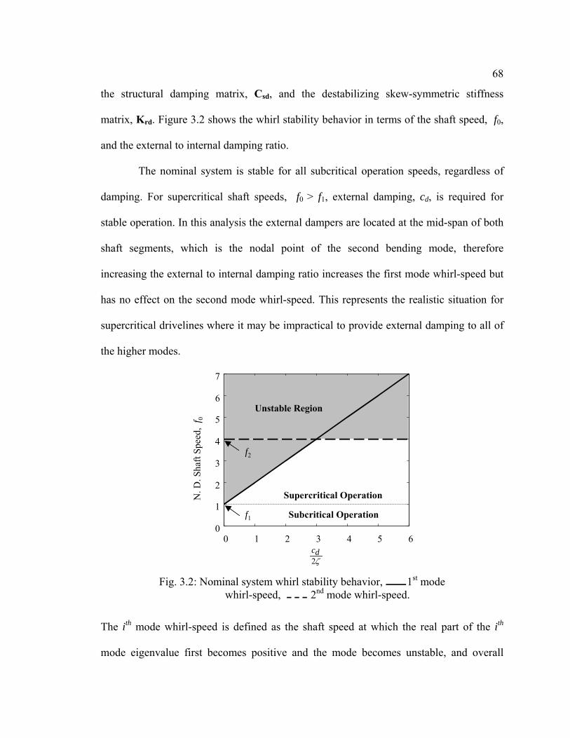
68

the structural damping matrix, Csd, and the destabilizing skew-symmetric stiffness

matrix, Krd. Figure 3.2 shows the whirl stability behavior in terms of the shaft speed, f0,

and the external to internal damping ratio.

The nominal system is stable for all subcritical operation speeds, regardless of

damping. For supercritical shaft speeds, f0 > f1, external damping, cd, is required for

stable operation. In this analysis the external dampers are located at the mid-span of both

shaft segments, which is the nodal point of the second bending mode, therefore

increasing the external to internal damping ratio increases the first mode whirl-speed but

has no effect on the second mode whirl-speed. This represents the realistic situation for

supercritical drivelines where it may be impractical to provide external damping to all of

the higher modes.

The ith mode whirl-speed is defined as the shaft speed at which the real part of the ith

mode eigenvalue first becomes positive and the mode becomes unstable, and overall

ζ2dc

0 1 2 3 4 5 60

1

2

3

4

5

6

7

Unstable Region

N. D

. Sha

ft Sp

eed,

f0

Supercritical Operation

f1

f2

Subcritical Operation

Fig. 3.2: Nominal system whirl stability behavior, 1st mode whirl-speed, 2nd mode whirl-speed.

69

whirl-speed is the slowest shaft at which whirl instability occurs. Equation (3.27) shows

the nominal system first and second mode whirl speeds, 1wf and 2wf , and the nominal

system overall whirl-speed, wf .

),min( , ,2 212211 wwww

dw ffffff

cf ==+=

ζ (3.27)

Since, in this case, external damping does not increase the second mode whirl-speed, the

largest achievable stable shaft speed range for the nominal system is 0 ≤ | f0 | < f2.

3.3.2 Full system stability

When misalignment and load-torque are present, the driveline dynamics are

described by the linear, periodic time-varying system given by (3.20). In this analysis, the

stability is determined numerically via Floquet theory by examining the eigenvalues of

the Floquet Transition Matrix (FTM), see Bolotin (1963). This technique is numerically

intensive, but deemed necessary to capture all the instability behavior of the system.

With Equation (3.20) recast in first order form and the forcing terms set to zero,

the system is written as

)()( and ][ with ,)( T**ttTt AAXXAX =+== ηη (3.28)

Where )(tA is the 2n x 2n periodic system matrix and X is the state vector. T is the N.D.

period, which is 0/ fT π= . Next, the FTM matrix, denoted by )( TΦ , is generated, where

])(....., ),( ),([)( 221 TTTT nxxx Φ = (3.29)

and ])(....., ),( ),([ 221 TTT nxxx are the 2n linearly independent solutions obtained by

numerically integrating Equation (3.28) from 0 to T with the following initial conditions

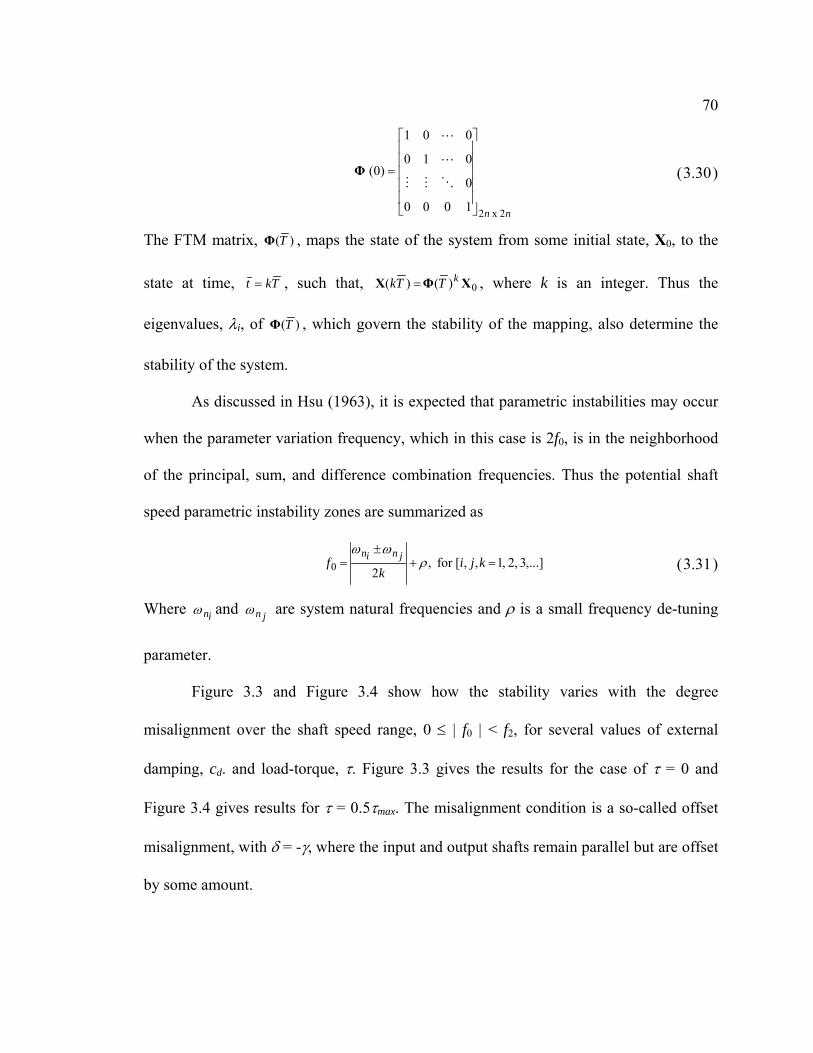
70

nn 2 x 21000

0

010

001

)0(

=OMM

L

L

Φ (3.30)

The FTM matrix, )( TΦ , maps the state of the system from some initial state, X0, to the

state at time, Tkt = , such that, 0)( )( XΦX kTTk = , where k is an integer. Thus the

eigenvalues, λi, of )( TΦ , which govern the stability of the mapping, also determine the

stability of the system.

As discussed in Hsu (1963), it is expected that parametric instabilities may occur

when the parameter variation frequency, which in this case is 2f0, is in the neighborhood

of the principal, sum, and difference combination frequencies. Thus the potential shaft

speed parametric instability zones are summarized as

,...]3 ,2 ,1,,[for ,20 =+±

= kji k

f jninρ

ωω(3.31)

Where inω and jnω are system natural frequencies and ρ is a small frequency de-tuning

parameter.

Figure 3.3 and Figure 3.4 show how the stability varies with the degree

misalignment over the shaft speed range, 0 ≤ | f0 | < f2, for several values of external

damping, cd. and load-torque, τ. Figure 3.3 gives the results for the case of τ = 0 and

Figure 3.4 gives results for τ = 0.5τmax. The misalignment condition is a so-called offset

misalignment, with δ = -γ, where the input and output shafts remain parallel but are offset

by some amount.

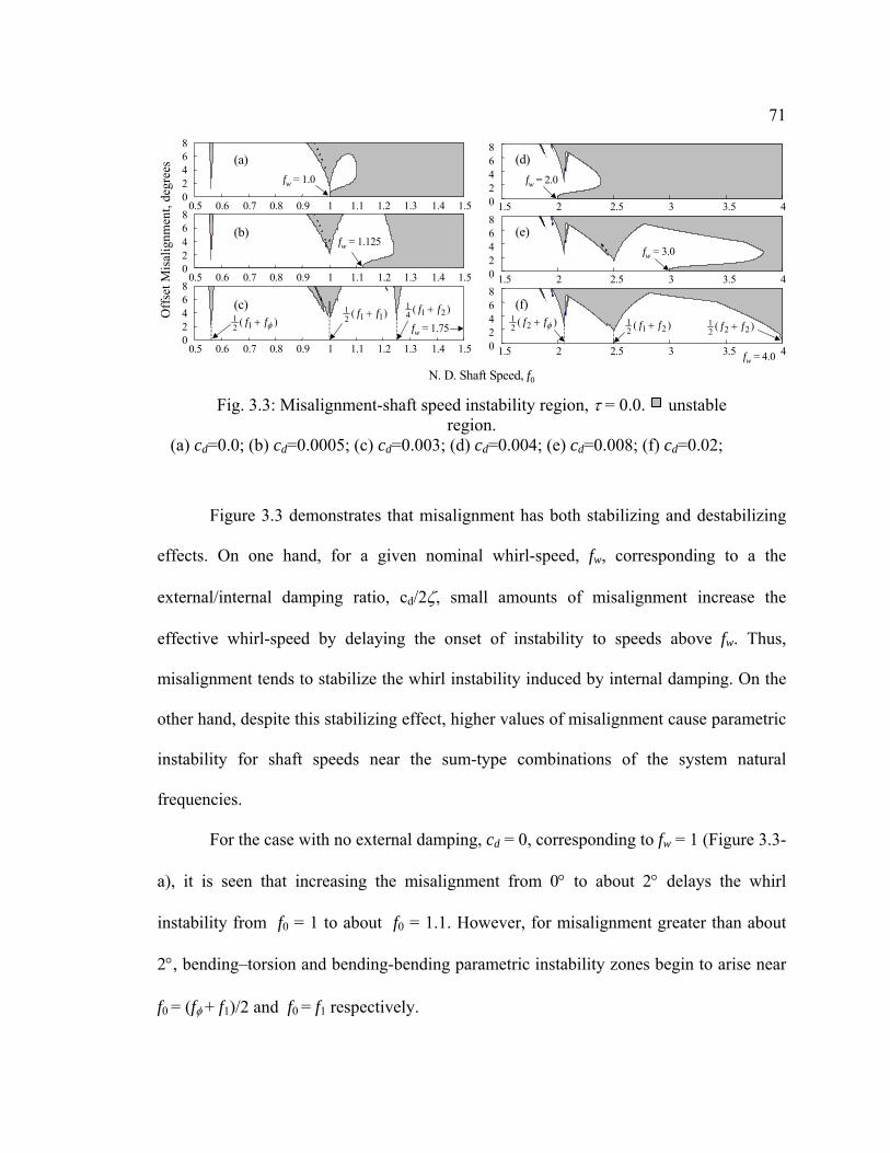
71

Figure 3.3 demonstrates that misalignment has both stabilizing and destabilizing

effects. On one hand, for a given nominal whirl-speed, fw, corresponding to a the

external/internal damping ratio, cd/2ζ, small amounts of misalignment increase the

effective whirl-speed by delaying the onset of instability to speeds above fw. Thus,

misalignment tends to stabilize the whirl instability induced by internal damping. On the

other hand, despite this stabilizing effect, higher values of misalignment cause parametric

instability for shaft speeds near the sum-type combinations of the system natural

frequencies.

For the case with no external damping, cd = 0, corresponding to fw = 1 (Figure 3.3-

a), it is seen that increasing the misalignment from 0° to about 2° delays the whirl

instability from f0 = 1 to about f0 = 1.1. However, for misalignment greater than about

2°, bendingtorsion and bending-bending parametric instability zones begin to arise near

f0 = (fφ + f1)/2 and f0 = f1 respectively.

N. D. Shaft Speed, f0

Off

set M

isal

ignm

ent,

degr

ees

02468

02468

02468

0.5 0.6 0.7 0.8 0.9 1 1.1 1.2 1.3 1.4 1.5

0.5 0.6 0.7 0.8 0.9 1 1.1 1.2 1.3 1.4 1.5

0.5 0.6 0.7 0.8 0.9 1 1.1 1.2 1.3 1.4 1.5

(a)

(b)

(c))( 12

1φff +

)( 1121 ff + )( 214

1 ff +

fw = 1.0

fw = 1.125

fw = 1.75

1.5 2 2.5 3 3.5 4

1.5 2 2.5 3 3.5 4

1.5 2 2.5 3 3.5 4

02468

02468

02468

(d)

(e)

(f))( 212

1 ff + )( 2221 ff +)( 22

1φff +

fw = 2.0

fw = 3.0

fw = 4.0

Fig. 3.3: Misalignment-shaft speed instability region, τ = 0.0. unstableregion.

(a) cd=0.0; (b) cd=0.0005; (c) cd=0.003; (d) cd=0.004; (e) cd=0.008; (f) cd=0.02;

72

For cases with non-zero external damping, cd > 0, small amounts of misalignment

continue to provide additional stabilization of the whirl boundary beyond the amount

provided by the external damping (Figure 3.3-b, d, e and f). Note, this phenomena would

also be seen in Figure 3.3-c, but in this plot cd is such that fw = 1.75, hence the whirl

boundary is outside the plot range for this graph. As the internal damping-induced whirl

instability boundary is shifted to higher shaft speeds with increasing cd, more

misalignment induced sum-type bending-bending and torsion-bending parametric

instability zones are revealed.

Bending-Bending Parametric Instability Zones:

ρρρρ +=++=++=+= 202121

02141

010 and )( and )( , ffffffffff(3.32)

Torsion-Bending Parametric Instability Zones:

ρρ φφ ++=++= )( and )( 221

0121

0 ffffff(3.33)

As seen in Equations (3.32) and (3.33), the bending-bending combination frequencies are

always supercritical, however the torsion-bending combination frequencies can be sub or

supercritical depending on the torsional natural frequency fφ. In this case, since fφ = 0.125,

the first torque-bending instability is subcritical, f0 = (fφ + f1)/2 = 0.5625 and the second

torque-bending instability is supercritical, f0 = (fφ + f2)/2 = 2.0625. Finally, it is also

apparent from Figure 3.3 that the parametric instability regions occurring at higher shaft

speeds have a wider frequency width for a given misalignment.

73

Figure 3.4, shows the effect of non-zero load-torque, τ, on the misalignment-shaft

speed instability regions. Here it is seen that, similar to misalignment, load-torque has

both stabilizing and destabilizing effects. On one hand, load-torque is stabilizing since it

tends to enhance the misalignment induced stabilization of the whirl instability. This can

be seen by comparing Figure 3.3 with Figure 3.4. This stabilization is most likely related

to the asymmetric stiffness coupling matrix, K0, which is a function of misalignment,

load-inertia, load-torque and shaft speed. This is consistent with the results from Zorzi

and Nelson (1977), where it was shown that bearing stiffness anisotropy delayed the

whirl instability to higher speeds. In this case it is not bearing stiffness anisotropy, rather,

it is an effective stiffness anisotropy created by misalignment and load-torque acting

through K0.

On the other hand, load-torque is destabilizing since it increases the size of the

misalignment induced torsion-bending instability. Furthermore load-torque causes


0.5 0.6 0.7 0.8 0.9 1 1.1 1.2 1.3 1.4 1.5

0.5 0.6 0.7 0.8 0.9 1 1.1 1.2 1.3 1.4 1.5

0.5 0.6 0.7 0.8 0.9 1 1.1 1.2 1.3 1.4 1.5

02468

02468

02468

(a)

(b)

(c))( 12

1φff +

)( 1121 ff + )( 214

1 ff +Off

set M

isal

ignm

ent,

degr

ees

fw = 1.0

fw = 1.75

fw = 1.125

1.5 2 2.5 3 3.5 4

1.5 2 2.5 3 3.5 4

1.5 2 2.5 3 3.5 4

02468

02468

02468

(d)

(e)

(f)

)( 2121 ff + )( 222

1 ff +)( 22

1φff +

fw = 2.0

fw = 3.0

fw = 4.0

Fig. 3.4: Misalignment-shaft speed instability region, τ = 0.5τmax unstable region. (a) cd=0.0; (b) cd=0.0005; (c) cd=0.003; (d) cd=0.004;

(e) cd=0.008; (f) cd=0.02;

74

instability at the bending-bending instability zones independent of the misalignment. This

is illustrated in Figure 3.4 where the bending-bending instability zones have a finite

frequency width even at zero misalignment.

3.3.3 Bending-Bending Parametric Instability

In this sub-section, since misalignment and load-torque independently cause

instability at shaft speeds near the sum-type bending-bending combination frequencies,

both kinds of instability are examined. Figure 3.5 and Figure 3.6 show the effect of

external damping on the load-torque and misalignment induced bending-bending

instability regions.

Figure 3.5 shows the misalignment induced bending-bending instability regions

with τ = 0 for several values of cd. The size of the misalignment instability regions near f0

= f1 and f0 = (f1 + f2)/4 are reduced by increasing the damping coefficient cd (Figure 3.5-

a). However, damping is not purely stabilizing for the instability region near f0 = (f1 +

f2)/2. In this case, damping increases the threshold of destabilizing misalignment, but also

increases the frequency width of the unstable region (Figure 3.5-b).

75

Figure 3.6 shows the load-torque induced bending-bending instability regions with δ = γ

= 0° for several values of cd. Here, again external damping tends to shrink the instability

region near f0 = f1 but causes spreading of the instability region near f0 = (f1 + f2)/2.


Off

set M

isal

ignm

ent,

degr

ees

0.9 1 1.1 1.2 1.3

0

2

4

6

8

12

11 =+ ff

25.14

21 =+ ff

1.8 2 2.2 2.4 2.6 2.8 3 3.20

2

4

6

0625.22

2=

+ φff

5.22

21 =+ ff

(a) (b)

Fig. 3.5: Effect of damping on misalignment induced bending-bending instability, τ = 0.0.

(a) cd = 0.002, cd = 0.02; (b) cd = 0.01, cd = 0.5;


2 2.2 2.4 2.6 2.8 30

0.2

0.4

0.6

0.8

1.0

maxτ

τ

5.22

21 =+ ff

0.8 0.9 1 1.1 1.20

0.2

0.4

0.6

0.8

1.0

12

11 =+ ff

(a) (b)

Fig. 3.6: Effect of damping on torque induced bending-bending instability,δ = γ = 0°. (a) cd = 0.002, cd = 0.01, cd = 0.02;

(b) cd = 0.01, cd = 0.2, cd = 0.5;

76

The spreading of the misalignment and load-torque instability regions near f0 = (f1 + f2)/2

could be related to the location of the external dampers. Since the dampers are at the mid-

span of the shafts, external damping is provided to the first bending modes only.

3.3.4 Torsion-Bending Parametric Instability

In this sub-section the behavior of the misalignment induced torsion-bending

instability zones is studied. Figure 3.7 and Figure 3.8 show the 1st and 2nd torque-bending

instability zones near f0 = (fφ + f1)/2 and f0 = (fφ + f2)/2 for several values of external

damping, cd, and load-torque, τ. As seen from the plots and as noted in sub-section 3.3.2,

the frequency width of both torsion-bending instability zones increases with load-torque.

However, load-torque alone, without misalignment, is not sufficient to cause torsion-

bending instability. Figure 3.7 shows that external damping, cd, causes spreading of the

1st torsion-bending instability region.

77

Off

set M

isal

ignm

ent,

degr

ees

21 φff +


0.5 0.54 0.58 0.620

2

4

6

8

(d)

0.5 0.54 0.58 0.620

2

4

6

8

(c)

0.5 0.54 0.58 0.620

2

4

6

8(b)

0.5 0.54 0.58 0.620

2

4

6

8(a)

Fig. 3.7: Effect of damping, torque and misalignment on 1st torsion-bending instability. cd = 0.0, cd = 0.04 (a) τ = 0.0; (b) τ = 0.25τmax;

(c) τ = 0. 5τmax; (d) τ =τmax


1.9 2 2.1 2.2 1.9 2 2.1 2.2

1.9 2 2.1 2.2 1.9 2 2.1 2.2

0

2

4

6

0

2

4

6

0

2

4

6

0

2

4

6

Off

set M

isal

ignm

ent,

degr

ees

22 φff +

(a)

(c)

(b)

(d)

Fig. 3.8: Effect of damping, torque and misalignment on 2nd torsion-bending instability. cd = 0.01, cd = 0.2 (a) τ = 0.0; (b) τ = 0.25τmax;

(c) τ = 0. 5τmax; (d) τ = τmax

78

Finally, since the external damper does not supply damping to either the torsion mode or

the 2nd bending mode, increasing cd has no effect on the 2nd torsion-bending instability,

see Figure 3.8.

3.4 Stability Analysis Summary and Conclusions

The previous sections show the effects of internal damping, external damping,

misalignment, load-inertia and load-torque on the stability of a segmented shaft

connected with U-Joint couplings operating at sub and supercritical speeds. The non-

dimensionalized driveline model includes both shaft bending and torsion flexibility along

with the kinematic effects of misalignment, coupling phase angles, and torque windup

angle between the U-Joint couplings. In the equation-of-motion, internal damping results

in both a damping matrix and a skew symmetric stiffness matrix, while the misalignment,

load-inertia and load-torque results in constant and periodic inertia, damping, and

stiffness coupling matrices, as well as forcing terms.

In the case with zero misalignment and zero load-torque, classic whirl instability

occurs for shaft speeds above some supercritical operating speed that depends on the ratio

of internal to external damping. Thus increasing external damping delays the onset of

whirl instability to higher shaft speeds. In the case studied in this analysis, external

damping can only delay whirl instability to the second critical speed, fw = f2, since the

mid-span dampers do not provide damping for the second bending mode. Thus, the range

shaft speed invested in the analysis is 0 ≤ | f0 | < f2.

79

When misalignment and load-torque are present, it is discovered that they both

have stabilizing and destabilizing effects. For a given level of external damping, cd, small

amounts of misalignment, δ and γ, and load-torque, τ, tend to delay the onset of whirl

instability beyond the nominal critical speed fcrit. This whirl stabilization is most likely a

consequence of the stiffness anisotropy created by the K0 coupling matrix.

Despite the whirl stabilization, misalignment and load-torque could create shaft

speed zones of parametric instability in the sum-type combination frequency regions.

Specifically, misalignment causes instability in both the bending-bending and torsion-

bending regions while load-torque only causes instability in the bending-bending regions.

Furthermore, even though load-torque by itself does not cause instability in the torsion-

bending regions, it tends to increases the frequency width of the torsion-bending

instability for a given level of misalignment.

The stability results for single U-Joint systems predict both torque induced

bending-bending instability and misalignment induced torsion-bending instability,

however misalignment induced bending-bending instability has not been identified in

previous research. This phenomena can be explained by the presence of misalignment

terms in the coupling matrices that allow periodic cross-coupling between bending modes

giving rise to instability in these modes.

In addition to stabilizing whirl instability, the effectiveness of using the external

mid-span dampers to stabilize the parametric instability is investigated. It is shown that

increasing the external damping, cd, causes some parametric instability regions to shrink

and others to spread. However, in both cases, increasing cd is beneficial since it increases

the destabilizing torque and misalignment threshold of the parametric instability zones.

80

Although the stability results are for a conventionally configured driveline with

no active control, the results give important insight into potential Configuration I control

algorithm designs, which must be stable in the presence of the misalignment and torque

induced NCV terms. In particular, since misalignment and torque NCV terms tend to

cause instability when shaft speed is near bending-bending or torsion-bending sum-type

combinations, a design constraint of the active control is that it should place the system

natural frequencies to avoid this condition. For a given supercritical operating speed,

assuming this constraint is satisfied together with the fact that misalignment and torque

both tend to stabilize whirl instability, the maximum amount of fixed-frame damping

needed for stability is the amount needed to stabilize the nominal system whirl. Thus, if

the combination frequencies are avoided, the control system can be designed based on the

nominal system, i.e. without the NCV terms. If the operating speed cannot be guaranteed

to be outside a given combination instability zone, the control system can maintain

stability by supplying sufficient damping to the particular modes involved. The damping

level can be designed off-line based on given misalignment and torque bounds.

81

Chapter 4

CONFIGURATION I: ROBUST ADAPTIVE VIBRATION CONTROL OF

MISALIGNED SUPERCRITICAL DRIVELINE WITH MAGNETIC BEARINGS

4.1 Introduction

As discussed in Chapter 1 and derived in Chapter 2, driveline misalignment and

load-torque together with NCV couplings introduce linear periodic parametric terms and

multiple harmonic forcing terms at integer multiples of shaft speed, NΩ0, N = [1,2,…nh].

Furthermore, as found in Chapter 3, misalignment and load-torque NCV effects are a

significant source of instability in segmented supercritical driveline systems. Due to the

significance of NCV effects on the stability and vibration response, it is clear that these

effects should be accounted for in the control law design for any AMB controlled,

segmented driveline system. However, NCV effects have not been considered in previous

AMB-rotor vibration control investigations. To advance the state-of-the-art, the main

objective of this chapter is to develop a robust active control law that can effectively

suppress both the synchronous imbalance response and the multi-harmonic vibration

induced by misalignment and torque NCV effects in misaligned AMB-driveline systems.

82

Many researchers have investigated active suppression of imbalance vibration

in various AMB-rotor systems. One very successful approach for suppressing imbalance

vibration is the open-loop synchronous adaptive vibration control (SAVC), Knospe, et al.

(1993). In this approach, given an AMB-rotor system with a feedback controller,

synchronous perturbation control inputs are generated and added to the feedback inputs.

These single frequency sinusoidal control inputs are synchronized with the shaft rotation

while the magnitude and phase are adjusted to minimize the imbalance response. This

adjustment is performed slowly relative to the decay of the rotor’s transient response, so

the process can be considered as the adaptation of a set of open-loop signals. Thus, the

system is stable as long as the original closed-loop system is stable and the perturbation

control inputs converge. The adaptation of the open-loop input is based on an estimate of

the Fourier influence coefficient mapping, yuT , from the control input to the response

output at frequency Ω. Since errors between the actual and estimated yuT matrix can

cause the open-loop adaptation process not to converge, both the convergence and

performance robustness with respect to several types of structured uncertainties in the yuT

matrix were explored. In particular, both operating speed and static rotor stiffness

uncertainty have been studied Knospe, et al. (1997).

Given the success of the SAVC approach in suppressing synchronous vibration of

linear time-invariant (LTIV) plants, one focus of this chapter is to extend this control

methodology to the more general case of periodically time varying (LPTV) plants with

multiple harmonic excitation, e.g. the AMB-NCV-driveline system. Specifically, in this

research, to ensure both stability and effective vibration suppression, a hybrid control

83

strategy is developed based on a decentralized PID feedback control which is

augmented with a slowly updating multi-harmonic adaptive vibration control (MHAVC).

The function of the PID feedback is to levitate the driveline and maintain closed-loop

stability, while the MHAVC input adapts to suppress the multi-harmonic response at the

shaft speed multiples, NΩ0, due to imbalance, misalignment and load-torque.

In this investigation, since misalignment and load-torque typically vary within

some operating range, the NCV terms are treated as periodic time-varying model

uncertainty. Thus, another focus of this chapter is to design the hybrid PID-MHAVC

control system in order to ensure stability and performance robustness with respect to

misalignment, load-torque and shaft imbalance uncertainties. The resulting robust PID-

MHAVC controlled AMB-NCV-driveline system stability and vibration performance is

investigated over a range of driveline operating conditions.

4.2 Segmented AMB-NCV Driveline System

Figure 4.1 is a schematic of the AMB controlled, segmented tailrotor driveline

with NCV couplings. Here, the fuselage structure is assumed to be subjected to a static

aerodynamic loading which produces a vertical-plane driveline misalignment, θv, and the

corresponding vertical-plane flexible coupling misalignments δ3, ξ3, and γ3. Refer to

Chapter 2 for details.

84

From the derivation in Chapter 2, the linear periodic time-varying equations-of-motion

for the AMB-NCV-driveline system in modal coordinates, 1mode ×ℜ∈ Nη (Nmode = 20),

about the statically misaligned equilibrium condition is given by (4.1).

[ ] [ ][ ] )()()( )(

)( )(

tuttt

tt

AMBIMBNCVGRAVNCVAMBTrd

NCVNCV

QFFFKKKKK

CGCMM

+++=+++++

++++

η

ηη L&&&( 4.1 )

Where the periodic parametric and forcing NCV terms and the synchronous shaft

imbalance are given by (4.2).

)cos()sin()()2cos()2sin()(

)2cos()2sin()()2cos()2sin()(

)2cos()2sin()(

0101

02020

02020

02020

02020

tttttt

tttttt

ttt

cs

cs

cs

cs

cs

Ω+Ω=Ω+Ω+=

Ω+Ω+=

Ω+Ω+=Ω+Ω+=

FFFFFFF

KKKKCCCC

MMMM

IMB

NCV

NCV

NCV

NCV

( 4.2 )

A

Lamb3

Lamb2

AMB2AMB3

AMB1

Lamb1 3-γ

3-δ

3-ξ vθ-

B

C

n2

n1

Fig. 4.1: Configuration I: segmented driveline with AMBs and NCV couplings.

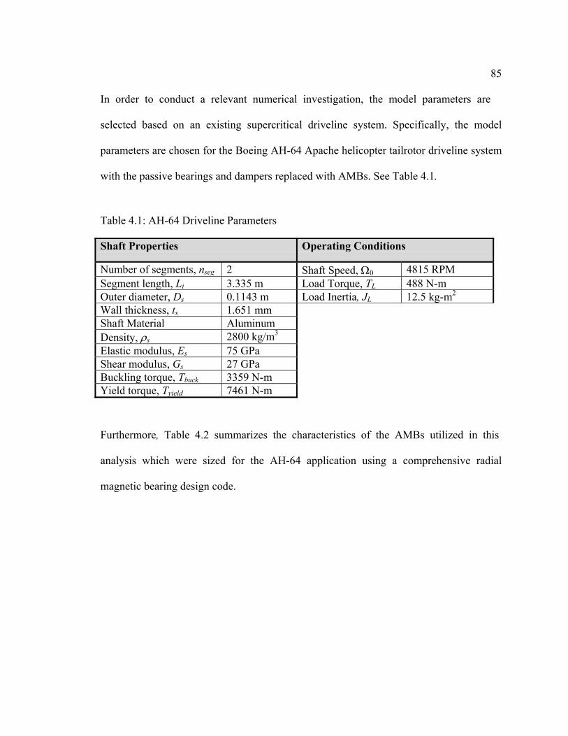
85

In order to conduct a relevant numerical investigation, the model parameters are

selected based on an existing supercritical driveline system. Specifically, the model

parameters are chosen for the Boeing AH-64 Apache helicopter tailrotor driveline system

with the passive bearings and dampers replaced with AMBs. See Table 4.1.

Furthermore, Table 4.2 summarizes the characteristics of the AMBs utilized in this

analysis which were sized for the AH-64 application using a comprehensive radial

magnetic bearing design code.

Table 4.1: AH-64 Driveline Parameters

Shaft Properties Operating Conditions

Number of segments, nseg 2 Shaft Speed, Ω0 4815 RPMSegment length, Li 3.335 m Load Torque, TL 488 N-mOuter diameter, Ds 0.1143 m Load Inertia, JL 12.5 kg-m2

Wall thickness, ts 1.651 mmShaft Material AluminumDensity, ρs 2800 kg/m3

Elastic modulus, Es 75 GPaShear modulus, Gs 27 GPaBuckling torque, Tbuck 3359 N-mYield torque, Tyield 7461 N-m

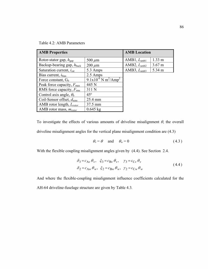
86

To investigate the effects of various amounts of driveline misalignment θ, the overall

driveline misalignment angles for the vertical plane misalignment condition are (4.3)

θv = θ and θw = 0 ( 4.3 )

With the flexible coupling misalignment angles given by (4.4). See Section 2.4.

, ,

, ,

C2B2A2

C3B3A3

wwwwww

vvvvvv

ccc

ccc

θγθξθδ

θγθξθδ

===

===( 4.4 )

And where the flexible-coupling misalignment influence coefficients calculated for the

AH-64 driveline-fuselage structure are given by Table 4.3.

Table 4.2: AMB Parameters

AMB Properties AMB Location

Rotor-stator gap, hgap 500 µm AMB1, Lamb1 1.33 mBackup-bearing gap, hback 200 µm AMB2, Lamb2 3.67 mSaturation current, isat 5.3 Amps AMB3, Lamb3 5.34 mBias current, ibias 2.5 AmpsForce constant, Gb 9.1x10-6 N m2/Amp2

Peak force capacity, Fmax 445 NRMS force capacity, Frms 311 NControl axis angle, θb 45°Coil-Sensor offset, dsens 25.4 mmAMB rotor length, Lrotor 37.5 mmAMB rotor mass, mrotor 0.645 kg

87

Finally, the imbalance loading is assumed to be due to a first-order sinusoidal bend or

run-out distribution along each shaft segment. The resulting shaft segment imbalance

load magnitude distribution is (4.5)

)/sin()( 20 iccsimb Lxemxf Ω= ( 4.5 )

where ecc is the eccentricity at the mid-span of each shaft segment. In this analysis ecc is

taken to be ecc = 2x10-4 m, which is a typical value for aluminum helicopter driveshafts,

Darlow, et al. (1990). Refer to Chapter 2 for further formulation details.

4.3 Active Control Law Structure

Figure 4.2 is block diagram of the closed-loop AMB-driveline system developed

in this investigation. 1 ×ℜ∈ dnd and 1 ×ℜ∈ znz are disturbance input and performance output

vectors. 1 ×ℜ∈ yny is a vector of transverse shaft displacements measured by the AMB

sensors, and 1 ×ℜ∈ unu is the AMB control input vector. Since each AMB has two

orthogonal axes of control and there are a total of 3 AMBs, ny = nu = 6.

Table 4.3: AH-64 Misalignment Influence Coefficients

Flex Coupling Vertical PlaneInfluence Coefficients

Horizontal PlaneInfluence Coefficients

A cvA = 0.748 cwA = 0.735B cvB = 0.498 cwB = 0.458C cvC = 0.249 cwC = 0.231

88

In this hybrid control strategy, the control input, u, consists of two components given by

),()()( tiututu MHAVCPID += ( 4.6 )

Here 1 ×ℜ∈ unPIDu is the input generated from an analog Proportional-Derivative-Integral

(PID) feedback control given by

IPID yyyu Idp KKK −−−= & with ∫= dtyyI ( 4.7 )

Where Kp = kpI, Kd = kdI and KI = kII are constant diagonal matrices with the

proportional, derivative and integral feedback gains kp, kd and kI. Furthermore,

1 ×ℜ∈ unMHAVCu is the multi-harmonic input generated by the Multi-Harmonic-Adaptive-

Vibration-Control (MHAVC) portion of the control law.

[ ]∑=

Ω+Ω+=hn

ncnsnMHAVC tnitniitiu

1000 )cos()()sin()()(),( uuu ( 4.8 )

Analog PIDController

+

PID Controlled System

AMB/NCVDriveline

Plant

Multi-Harmonic AdaptiveVibration Control

A/DD/A

z

yu

uPID

d

uMHAVC

Fig. 4.2: Driveline with hybrid PID/Multi-Harmonic Adaptive Vibration Control.

89

Here nh is the number of harmonics and )(0 iu , )(isnu and 1 )( ×ℜ∈ uncn iu for

n∈[1,2,…nh] are the ith updated Fourier coefficient vectors which are adapted to suppress

steady-state vibration.

Next, since the PID feedback gains are constant, the PID controlled AMB-

driveline sub-system in Figure 4.2 can be written as the LPTV state-space descriptor

system (4.9).

xCz

xCytuBtdBxtAxtE

z

y

MHAVCud

=

=

++= )()()()( &

( 4.9 )

Here 1][ ×ℜ∈= xnTI

TT yx ηη & is the closed-loop state vector, dnxndB ×ℜ∈ and

unxnuB ×ℜ∈ are the disturbance and control input distribution matrices and xnzn

zC ×ℜ∈

and xnynyC ×

ℜ∈ are performance and measured output state-space observation matrices.

Furthermore, the periodic system and derivative matrices, xnxnp tATtA ×ℜ∈=+ )()( and

xnxnp tETtE ×ℜ∈=+ )()( , each with period 0Ω=πpT , are written as (4.10).

)2cos()2sin()( 02020 tEtEEItE cs Ω+Ω++=

)2cos()2sin()( 02020 tAtAAAtA csn Ω+Ω++=(4.10)

In terms of Equations (4.1), (4.2) and (4.7), the matrices in (4.9) and (4.10) are

90

( ) ( )

=

=

=

−−=

−−=

+−++−=

−+−++−=

00000000

,00000000

,00000000

0000000

,0000000

,0000)()(000

00

00

2200

220

c2s2

c2c2s2s200rdT

AMB

IAMBAMBdAMBAMBpAMBAMB

MMM

CKCKCGKKK

PKQPKQCPKQKK

I

cs

cs

n

EEE

AAA

A

(4.11)

Where An represents the nominal PID controlled AMB-driveline system i.e. for the

operating conditions [Ω0 = 0, TL = 0, θ = 0]. With mode Nyn ×ℜ∈AMBP defined as the AMB

sensor observation matrix in modal coordinates, i.e. η AMBP=y . Finally, the control and

disturbance matrices in (4.9) are

=

AMBQ0

uB and

=

c2s2c1s10 FFFFF0

dB (4.12)

with corresponding disturbance input vector

[ ]Ttttttd )2cos()2sin()cos()sin(1)( 0000 ΩΩΩΩ= (4.13)

which is expanded in terms of the Fourier coefficient vectors 0d , snd and 1 ×ℜ∈ dncnd (nd

= 5) for n∈[1,2,…nh] as

[ ]∑=

Ω+Ω+=hn

ncnsn tntntd

1000 )cos()sin()( ddd (4.14)

In order to develop the MHAVC portion of the controller for the PID controlled AMB-

driveline system in (4.9), a Fourier influence coefficient mapping from the control input

to the system output must be obtained. However, since the equations in (4.9) are time-

varying, the Fourier influence coefficient mapping does not have a convenient closed-

91

form representation. Therefore an approximate version is obtained via a truncated

harmonic balance approach.

Assuming the PID controlled AMB-driveline system in (4.9) is Bounded-Input-

Bounded-Output (BIBO) stable (guaranteed through PID robust design in Section 4.4.1)

and given the multi-harmonic control and disturbance inputs uMHAVC(t) and d(t) in (4.8)

and (4.14), the steady-state x and x& are approximated as

[ ]∑=

Ω+Ω+=hn

ncnsn tntntx

1000 )cos()sin()( xxx

[ ]∑=

Ω−ΩΩ=hn

ncnsn tnntnntx

1000 )sin()cos()( xx&

(4.15)

and the steady-state outputs y and z are

[ ]∑=

Ω+Ω+=hn

ncnsn tntnty

1000 )cos()sin()( yyy

[ ]∑=

Ω+Ω+=hn

ncnsn tntntz

1000 )cos()sin()( zzz

(4.16)

After substituting (4.8) and (4.14)-(4.16) into (4.9) and equating like harmonics with nh =

4, the following truncated Fourier influence coefficient representation is obtained

=

DU

TTTT

ZY

zdzu

ydyu (4.17)

where, 1 ×ℜ∈ dnfnD , 1 ×

ℜ∈ unfnU , 1 ×ℜ∈ ynfnY and 1 ×

ℜ∈ znfnZ , with 12 += hf nn , are the combined

Fourier coefficient vectors

92

TTc

Ts

Tc

Ts

Tc

Ts

Tc

Ts

T

TTc

Ts

Tc

Ts

Tc

Ts

Tc

Ts

T

TTc

Ts

Tc

Ts

Tc

Ts

Tc

Ts

T

TTc

Ts

Tc

Ts

Tc

Ts

Tc

Ts

T

Z

Y

U

D

=

=

=

=

443322110

443322110

443322110

443322110

zzzzzzzzz

yyyyyyyyy

uuuuuuuuu

ddddddddd

(4.18)

With the influence coefficient matrices in (4.17) unfnynfnyuT ×

ℜ∈ , dnfnynfnydT ×

ℜ∈ ,

unfnznfnzuT ×

ℜ∈ , dnfnznfnzdT ×

ℜ∈ given by

[ ] [ ]

[ ] [ ]

Ψ

=

Ψ

=

Ψ

=

Ψ

=

−−

−−

d

d

z

z

zd

u

u

z

z

zu

d

d

y

y

yd

u

u

y

y

yu

B

B

C

CT

B

B

C

CT

B

B

C

CT

B

B

C

CT

OOOO

OOOO

11

11

,

,

(4.19)

Where the matrix xnfnxnfnLIdpn Tkkk ×

ℜ∈Ω∆Ψ+Ψ=Ψ ),,(),,( 0 θ in terms of the system

matrices in (4.9) and (4.10) is

−ΩΩ−−

−ΩΩ−−

−ΩΩ−−

−ΩΩ−−

−

=Ψ

n

n

n

n

n

n

n

n

n

n

AIIA

AIIA

AIIA

AIIA

A

0

0

0

0

0

0

0

0

4000000040000000

003000000030000000002000000020000000000000000000000000

(4.20)

and

93

Ω+

Ω+−

Ω+−Ω+

Ω−−Ω+−

Ω−−−

Ω−−−+Ω+−

−Ω−−Ω++−

Ω+−−

=∆Ψ L

202

202

20

220

2

20

220

2002

02

20

20

200

2

200

220

20

202

0

2000

2000

02222

0

02222

0

20000

022

)2

(2

0

0)2

(222

02

00

cs

sc

sccs

csscc

s

sccs

cssc

cs

EA

EA

EAEA

EAEAEA

AA

EAA

EE

A

EE

AEAA

EA

A

−ΩΩ+−

Ω−−Ω−−

−ΩΩ−−

Ω−−Ω+−−

Ω−Ω−−Ω−

Ω−−Ω+−

Ω−Ω−−

Ω−−

000202

000202

000

000

202

202

0

202

202

00

20

220

2

20

220

2

202

4002

4002

00300030

22

22

00

22

22

002

002

322

32

0

002

322

32

0

00002

AEEA

EAEAAE

EA

EAEAA

EAEAE

EAEA

EAEA

EA

sc

cs

sc

cs

cs

sc

sccs

cssc

sc

(4.21)

Here nΨ is the nominal system contribution and ∆Ψ is due to Ω0 , TL , and θ dependent

terms. From the Fourier influence coefficient representation in (4.17), define the baseline

response as DTY ydPID = and DTZ zdPID = which is just the steady-state response of the

PID controlled AMB-driveline system without any MHAVC input, (i.e. U = 0). In this

control strategy, the MHAVC input, U, will be updated slowly to allow the system to

reach a steady-state after each update. The steady-state response after the ith MHAVC

update is

PIDiyui YUTY += and PIDizui ZUTZ += (4.22)

94

In order for the MHAVC to suppress driveline vibration, the MHAVC update law is

obtained through least-squares minimization of the following objective function Ji. Refer

to Appendix D for derivation details.

iT

iiT

ii RUUWYYJ += with fnunperf IwW = and fnuneff IwR = (4.23)

Here fyfy nnnnW ×ℜ∈ are fufu nnnnR ×ℜ∈ vibration performance and control effort weighing

matrices. Where wperf and weff (m2/Amp) are scalar design variables which penalize shaft

vibration and MHAVC control effort respectively. Based on least-squares minimization

of Ji the MHAVC update law is

][][ 11 iiyu

Tyuyu

Tyui YUTWTRWTTU −+= −

+ (4.24)

In order to implement the MHAVC update law, the multi-harmonic transfer matrix, Tyu,

must be known. However, the exact Tyu cannot be utilized since, as shown in (4.19)-

(4.21), it depends on uncertain operating conditions, [Ω0, TL, θ]. Therefore, some

approximate version, yuT , must be utilized and the implemented MHAVC update law

becomes.

]ˆ[ˆ]ˆˆ[ 11 iiyu

Tyuyu

Tyui YUTWTRTWTU −+= −

+ (4.25)

Since errors between the actual yuT and the estimate, yuT , can cause (4.25) not to

converge, MHAVC convergence robustness must be considered in the control design.

95

4.4 Robust PID-MHAVC Controller Design

Conceptually, in the hybrid PID-MHAVC control system, the function of the PID

feedback is to ensure stable levitation of the AMB-driveline while the MHAVC adapts

and converges to suppress the steady-state vibration. Since the MHAVC input is confined

to slow adaptation rates relative to the transients of the PID controlled AMB-driveline

system in (4.9), the MHAVC is essentially an adapted open-loop input which does not

affect BIBO stability. Therefore, the PID and MHAVC portions of the hybrid PID-

MHAVC law can be designed sequentially in two design steps. In step I, Sub-Section

4.4.1, the PID gains, kp, kd and kI, are selected to ensure robustly stable levitation of the

AMB-driveline system. In second step, Sub-Section 4.4.2, the MHAVC objective

function weightings, wperf and weff, are designed based on convergence requirements.

From a control design point-of-view, the driveline operating conditions, [Ω0, TL,

θ] are assumed to be uncertain within some range. Thus, the operating condition

uncertainty space, Vu, is defined as

[ ]maxminmaxminmax0min ,, θθθ ≤≤≤≤Ω≤Ω≤Ω= LLLu TTTV (4.26)

and the PID-MHAVC law must be designed so that the overall system is robust with

respect to these uncertainties. In particular, Table 4.4 gives the operating condition

uncertainty bounds considered in this analysis.

96

4.4.1 Step I, Robust PID Feedback Design

In this sub-section, the PID feedback controller gains which guarantee BIBO

stability of the AMB-driveline system with respect to driveline operating conditions is

designed. At a given operating condition, [Ω0, TL, θ ], and for a given PID control design,

[kp, kd, kI], the PID controlled AMB-driveline system (4.9) is LPTV, hence, its BIBO

stability is characterized by Floquet theory. Specifically, stability is determined by

evaluating the eigenvalues of the Floquet Transition Matrix of (4.9) which is

])(....., ),( ),([)( 21 pxnppp TxTxTxT =Φ (4.27)

Where ])(....., ),( ),([ 21 pxnpp TxTxTx are the nx linearly independent solutions at t =

Tp obtained by integrating xtAtEx )()(1−=& from 0 to Tp with initial conditions I=Φ(0) .

Using this, the BIBO stability state, s, for a given PID controller design and operating

condition is defined as

<Φ

≥Φ=Ω

(stable) 1 )]([ if 1

(unstable) 1)]([ if 0 ),,,,,( 0

p

pIdpL

T

TkkkTs

ρ

ρθ (4.28)

Table 4.4: Operating Condition Uncertainty Bounds

Operating Condition Minimum Value Maximum Value

Operating speed, Ω0 Ωmin = 0 RPM Ωmax = 5000 RPMLoad torque, TL TLmin = 0 N-m TLmax = 2500 N-mMisalignment, θ θmin = 0° θmax = 8°

97

where ] [ρ is the spectral radius. Next, as a metric for PID control design, the robust

stability index, [0≤ SPID ≤1], is defined in terms of the stability state, s, over the operating

parameter space Vu.

∫∫∫ ΩΩ−−Ω−Ω

≡

uVLIdpL

LLIdpPID ddTdkkkTs

TTkkkS θθ

θθ 00minmaxminmaxminmax

),,,,,())()((

1),,( (4.29)

For a given PID control design, SPID quantifies the BIBO stability robustness of (4.9) over

the operating condition parameter space Vu . Where SPID = 1 indicates stability over the

entire Vu space i.e. robust stability. Figure 4.3 shows how SPID varies with the active

stiffness and damping gains, kp and kd, for a given integrator gain kI = 1000 Amp/m-sec.

0 200 400 600 800 10003

3.5

4

4.5

5

5.5

6

6.5 1.0

0.9

0.8

0.7

0.6

0.5

0.4

0.3

0.1

0.1

0.0

Robust BIBOStability Region

Log10[kp](P Gain),Amp/m

kd (D Gain), Amp-sec/m

[ ]°≤≤≤≤≤Ω≤= 800RPM 50000 max0 θLLu TTV

SPID

*pk

*dk

SPID=1

Fig. 4.3: Robust stability index, SPID vs. kp and kd with kI. = 1000 Amp/m-sec.

98

This analysis shows that there is a single range of stiffness and damping gains, [2982 ≤

kp ≤ 32320, 12 ≤ kd ≤ 238] with kI = 1000 Amp/m-sec, which guarantee robust BIBO

stability of the AMB-NCV driveline system over the operating condition space, Vu.

Furthermore, the results show that, for kp < 2982 Amp/m, SPID = 0, which indicates that

the closed-loop system is unstable over the entire operating parameter space. This is a

result of the negative magnetic levitation stiffness, KAMB, which must be counter-acted

by a sufficiently large active stiffness gain, kp, for stability. To proceed with the analysis,

the final robust PID controller design [kp = kp*, kd = kd* and kI = kI*], is selected by

choosing the gains from the mid-point of the robust design region. See Table 4.5.

Additionally, Table 4.6 shows the first few closed-loop natural frequencies of the

nominal PID controlled AMB driveline system using the robust PID gains, [kp = kp*, kd =

kd*, kI = kI*], in the control law.

Table 4.5: Robust PID Feedback Design

Final Design Gains Allowable Operating Condition Range

Stiffness Gain, kp* 15000 Amp/m Ωmin = 0 RPM Ωmax = 5000 RPMDamping Gain, kd* 175 Amp-sec/m TLmin = 0 N-m TLmax = 2500 N-mIntegrator Gain, kI* 1000 Amp/m-sec θmin = 0° θmax = 8°

99

4.4.2 Step II, Robust MHAVC Design

In this sub-section, the MHAVC control effort weighting parameter, weff, in the

objective function (4.23), is designed to guarantee robust convergence of the open-loop

MHAVC input with respect to the driveline operating condition uncertainty space, Vu. To

implement the MHAVC portion of the control, the transfer matrix estimate, yuT , used to

compute the MHAVC update law in (4.25) is based on the nominal PID controlled AMB-

driveline system, i.e. with PID gains [kp = kp*, kd = kd*, kI = kI*] and operating

conditions [Ω0 = 0, TL = 0, θ= 0].

Ψ

=≡−

===

===Ωu

u

Idpn

y

y

IkIkdkdkpkpkLTyuyu

B

Bkkk

C

CTT OO

1***

* ,* ,*0 ,0 ,00

),,( ˆθ (4.30)

Thus, the error between yuT and yuT only depends on the uncertain operating condition

parameters [Ω0 , TL, θ].

Table 4.6: Nominal PID/AMB Driveline Closed-Loop Natural Frequencies

Shaft Bending Modes (Pairs) Shaft Torsion Modes

1st Mode 86.5 Hz 1st Shaft Torsion 4.1 Hz

2nd Mode 133.4 Hz 2nd Shaft Torsion 176.8 Hz

3rd Mode 212.1 Hz

4th Mode 243.7 Hz

100

Since the PID controlled AMB-driveline system (4.9) is guaranteed BIBO

stable by use of [kp = kp*, kd = kd*, kI = kI*], the convergence of the open-loop MHAVC

input is governed by the following condition.

[ ][ ] eConvergenc 1

Divergence 1

<Λ

≥Λ

ρ

ρ with ]ˆ[ˆ]ˆˆ[ 1

yuyuT

yuyuT

yu TTWTRTWT −+=Λ − (4.31)

Where the MHAVC Convergence Metric, [ ]Λρ , is defined as the maximum eigenvalue of

the matrix Λ. Also, the converged MHAVC input and response ci UU → and ci YY → with

∞→i are given by

PIDT

yuyuT

yuc WYTRWTTU ˆ]ˆ[ 1−+−= and PIDcyuc YUTY += (4.32)

Refer to Appendix E for details.

To asses the MHAVC convergence robustness with respect to the operating

condition uncertainty space, Vu, the MHAVC Robust Convergence Metric is defined as

Λ= ),(sup),( effperf

uVeffperf wwww ρσ (4.33)

According to this definition, σ < 1 indicates robust convergence, i.e. the MHAVC input

converges at all operating conditions in Vu.

To proceed with the design, the performance weighting parameter, wperf, is chosen

as wperf = 1 and the MHAVC control effort weighting parameter, weff, is selected to ensure

robustness. Figure 4.4 shows the MHAVC Convergence Metric, [ ]Λρ , versus shaft speed

at two different misalignment and load torque operating conditions [TL, θ ] for two

amounts of MHAVC control effort penalty weighting weff.

101

This figure shows that TL and θ tend to cause divergence of the MHAVC adaptation

process, (4.25), at certain shaft operating speeds. Misalignment and torque tend to affect

the convergence at different speeds. Comparing Figure 4.4 (a) and (b) shows the effect

of two different load-torque levels (TL = TLmax and TL = 0.5TLmax) with θ = 4°. In this case,

misalignment, θ, tends to cause divergence near Ω0 = 1500 and Ω0 = 1900 RPM while the

load-torque, TL, tends to cause divergence at higher speeds, Ω0 > 3000 RPM. This figure

also shows that increasing the MHAVC control effort penalty weighing, weff, tends to

reduce [ ]Λρ at all operating speeds Ω0, thus improving the MHAVC convergence

characteristics.

To further explore the MHAVC convergence behavior, Figure 4.5 shows the

effect of driveline misalignment, θ, and shaft speed, Ω0, for max0 LL TT ≤≤ on the

Controller Parameters:PID-MHAVC withweff = 0 µm2/Amp

PID-MHAVC withweff = 1000 µm2/Amp

0

0.5

1

1.5

2

[ ]Λρ DivergenceConvergence

(a)

0

0.5

1

1.5

2

Shaft Speed Ω0 , RPM

[ ]Λρ DivergenceConvergence

(b)PID Gains[kp=kp

*, kd=kd* , kI=kI

*]

1000 2000 3000 4000 50000

1000 2000 3000 4000 50000

Fig. 4.4: MHAVC Convergence Metric vs. shaft speed for weff = 0 and weff = 1000; (a)

[TL = 0.5TLmax, θ = 4°]; (b) [TL = TLmax, θ = 4°].

102

MHAVC convergence for several values of weff. Here the non-shaded regions are

regions where [ ]Λρ < 1.

Misalignment causes the MHAVC update law to diverge near various shaft speeds

similar to the parametric instability regions in Chapter 3, where the system natural

frequencies are now the closed-loop eigenvalues of the nominal PID controlled AMB-

driveline system. By comparing the convergence regions for the three different values of

weff in Figure 4.5, it is clear that weff has a significant impact on the convergence. This is

further illustrated in Figure 4.6, which is a plot of the convergence robustness metric, σ

versus weff for two different levels of operating condition uncertainty.

1000 2000 3000 4000 5000

02468

02468

02468

0

0

0

Shaft Speed Ω0 , RPMMHAVCDivergence

Mis

alig

nmen

t θ ,

degr

ees

1000 2000 3000 4000 5000

1000 2000 3000 4000 5000

PID-MHAVC withkp=kp

*, kd=kd* , kI=kI

*

weff = 0 µm2/Amp

PID-MHAVC withkp=kp

*, kd=kd* , kI=kI

*

weff = 100 µm2/Amp

PID-MHAVC withkp=kp

*, kd=kd* , kI=kI

*

weff = 1000 µm2/Amp

Fig. 4.5: θ - Ω0 MHAVC convergence regions for various weff with max0 LL TT ≤≤ .

103

For a given level of operating condition uncertainty, convergence robustness (σ < 1) is

guaranteed by selecting a sufficiently large value of weff, i.e. criteffeff ww > . However, since

weff penalizes the MHAVC control effort, and thus limits the magnitude of the MHAVC

inputs, the vibration performance with respect to weff also needs to be considered.

4.5 PID-MHAVC Performance Analysis

In this section, the vibration performance and required control currents for the

hybrid PID-MHAVC controlled AMB-driveline system are analyzed over a range of

driveline operating conditions. In particular, Sub-Section 4.5.1 investigates the effect of

RobustConvergence

Metric

MHAVC Control Effort Penalty, weff µm2/Amp

DivergenceConvergence

0

1

2

3

1x102 1x103 1x104 1x105 1x106 1x107 1x108 1x109 1x1010 1x1011

criteffw

Operating Condition Range:

)( effwσ

°≤≤≤≤≤Ω≤= 80,0 RPM, 50000 max0 θLLu TTV

°≤≤≤≤≤Ω≤= 40,0 RPM, 50000 max0 θLLu TTV

Fig. 4.6: MHAVC Robust Convergence Metric vs. MHAVC control effort weighting.

104

weff on the converged steady-state response, while Sub-Section 4.5.2 focuses on signal

processing implementation of the MHAVC and the transient time-domain response.

4.5.1 Steady-State Performance

To evaluate the PID-MHAVC performance, (4.32) in conjunction with (4.16) is

used to compute the converged, steady-state, shaft vibration and control current response

vectors y(t) and u(t). Furthermore, to asses the overall steady-state vibration and control

currents, the following scalar RMS and peak vibration and control current performance

metrics are defined as

∑ ∫∑ ∫==

==un

i

Ti

u

yn

i

Ti

ydttu

Tnidtty

Tny

1 0

2rms

1 0

2rms )(11 and )(11 (4.34)

and

=

=

<<<<<<<<)]([supsup and )]([supsup

10max

10max tuityy i

uniTti

yniTt(4.35)

where T = 2π/Ω0 is the fundamental period of the response.

Using the expressions in (4.35), Figures 4.7 and 4.8 show the worst-case shaft

vibration response and worst-case AMB control currents over several operating condition

ranges, Vu, versus the MHAVC control effort weighting design parameter weff.

105

For lower values of weff, near the minimum value required for convergence, criteffw ,

Figure 4.7 shows that the MHAVC input is very effective at suppressing shaft vibration


0

50

100

150

200

250

1x102 1x103 1x104 1x105 1x106 1x107 1x108 1x109 1x1010 1x1011

Backup-BearingGap Clearance

µ m

criteffw

°≤≤≤≤

≤Ω≤=

200

RPM 50000

max

0

θLLu TTV


MHAVCDivergence

°==≤Ω≤

=0

m-N 0RPM 50000 0

θLu TV

°≤≤≤≤

≤Ω≤=

400

RPM 50000

max

0

θLLu TTV

PID Baseline

PID Baseline

maxsup yuV

PID-MHAVC with [kp=kp*, kd=kd

* , kI=kI*]

m 200 y,EccenticitShaft µ=cce

PID Baseline

Fig. 4.7: PID-MHAVC/AMB-driveline converged response; worst-case vibration.

0

0.5

1

1.5

2

2.5

3


1x102 1x103 1x104 1x105 1x106 1x107 1x108 1x109 1x1010 1x1011

criteffw

Amps

°≤≤≤≤

≤Ω≤=

200

RPM 50000

max

0

θLLu TTV


m 200 y,EccenticitShaft µ=cce

MHAVCDivergence

°==≤Ω≤

=0

m-N 0RPM 50000 0

θLu TV

°≤≤≤≤

≤Ω≤=

400

RPM 50000

max

0

θLLu TTV

PID Baseline

PID Baseline

maxsup iuV

PID-MHAVC with [kp=kp*, kd=kd

* , kI=kI*]

Bias Current

PID Baseline

Fig. 4.8: PID-MHAVC/AMB-driveline response; worst-case control current.

106

over the entire range of operating conditions, Vu. In particular, the shaft vibration is

maintained well below the backup-bearing air-gap clearance threshold. Since no

knowledge of the imbalance, misalignment or load-torque is utilized in the

implementation of the control, the hybrid PID-MHAVC control strategy developed here

achieves robust performance. Furthermore, Figure 4.8 shows that the required control

currents are near or below the bias current level, and thus the control is feasible with the

magnetic bearings considered in this analysis. Finally, as expected, when weff is increased,

Figures 4.7 and 4.8 show that the vibration and current responses approach the PID

baseline values.

Figures 4.9 and 4.10 show the RMS shaft vibration and current, yrms and irms, at

three different operating conditions and three different control settings versus the shaft

speed. For the case with just synchronous imbalance excitation at frequency Ω0 and no

misalignment or load-torque, i.e. [ecc > 0, TL=0 N-m, θ=0°], there are no resonance peaks

in the response. This is because the closed-loop natural frequencies, ωn, of the nominal

PID controlled AMB-driveline system with [kp = kp*, kd = kd*, kI = kI*], are placed

above the maximum shaft speed i.e. ωn > Ω0. However, for cases with TL > 0 and θ > 0,

resonances are excited by the 2Ω0 and 4Ω0 super-synchronous NCV excitations. In this

case, the peak vibration amplitudes occur for shaft speeds near ¼ and ½ multiples of the

closed-loop natural frequencies, i.e. for Ω0 = ωn/4 and Ω0 = ωn/2. Despite this, Figure 4.9

shows that the PID-MHAVC achieves significant vibrations suppression across the shaft

speed range.

107

01000

20003000

40005000

0

20

40

60

80

100

yrms, µ m

ecc = 200 µ mTL = TL max

θ = 2.5° ecc = 200 µ mTL = 0.5TL max

θ = 2.5° ecc = 200 µ mTL = 0 N-mθ = 0°

Shaft Speed Ω0 , RPM

Controller Parameters:

PID-MHAVC withweff = 1x105 µm2/Amp

PID


PID Gains [kp=kp*, kd=kd

* , kI=kI*]

Fig. 4.9: PID-MHAVC/AMB-driveline response; RMS shaft vibration.

irms, Amps

Shaft Speed Ω0 , RPM01000

20003000

40005000

0

0.2

0.6

1

1.4

1.8

ecc = 200 µ mTL = TL maxθ = 2.5° ecc = 200 µ m

TL = 0.5TL maxθ = 2.5° ecc = 200 µ m

TL = 0 N-mθ = 0°

Controller Parameters:


PID


PID Gains [kp=kp*, kd=kd

* , kI=kI*]

Fig. 4.10: PID-MHAVC/AMB-driveline response; RMS control current.

108

Figure 4.10 shows that the control current magnitudes required by the PID-MHAVC

only exceed the PID baseline values near resonance. Thus, for shaft speeds operating

away from resonance, PID-MHAVC achieves significant vibration suppression with

negligible increases in control current magnitude.

To examine the contributions of the individual vibration and control current

response harmonics at frequencies Ω0, 2Ω0, 3Ω0 and 4Ω0, Figures 4.11 and 4.12 give the

baseline PID and PID-MHAVC controlled steady-state shaft vibration and control current

response harmonic amplitudes versus shaft speed, Ω0, for a particular ecc and [TL , θ ]

operating condition at AMB1.

Operating Conditions:


θ = 6.0°

Controller Parameters:PID


PID Gains [kp=kp

*, kd=kd* , kI=kI

*]

0 1000 2000 3000 4000 5000

0 1000 2000 3000 4000 5000

0 1000 2000 3000 4000 5000

0 1000 2000 3000 4000 5000

020406080

0

100

200

300

0

0.5

1

0

10

20

Shaft Speed Ω0, RPM

Vib

ratio

n A

mpl

itude

, µm

Ω0 Harmonic(Synchronous)

2Ω0 Harmonic

3Ω0 Harmonic

4Ω0 Harmonic

Fig. 4.11: PID-MHAVC/AMB-driveline vibration harmonics at AMB1.

109

Here, the synchronous portion of the response at Ω0 is due to the shaft imbalance and

the super-synchronous response at 2Ω0, 3Ω0 and 4Ω0 is due to the misalignment and load-

torque NCV effects. This figure also demonstrates that the PID-MHAVC effectively

suppresses the vibration at each of the harmonics.

Figure 4.12 shows that the PID-MHAVC only requires more control current than the

baseline PID controlled system near certain critical speeds.

Finally, Figures 4.13 and 4.14 show the peak vibration amplitude, ymax, and peak

control current, imax, versus misalignment at Ω0=4815 RPM, which is the actual shaft

operating speed of the AH-64 Apache tailrotor driveline. Since Ω0=4815 RPM is not at

0 1000 2000 3000 4000 5000

0 1000 2000 3000 4000 5000

0 1000 2000 3000 4000 50000

0.02

0.04

0 1000 2000 3000 4000 5000

0

0.2

0.4

0

2

4

0

0.2

0.4

Shaft Speed Ω0, RPM

Con

trol

Cur

rent

, Am

ps


2Ω0 Harmonic

3Ω0 Harmonic

4Ω0 Harmonic

Operating Conditions:


θ = 6.0°

Controller Parameters:PID


PID Gains [kp=kp

*, kd=kd* , kI=kI

*]

Fig. 4.12: PID-MHAVC/AMB-driveline control current harmonics at AMB1.

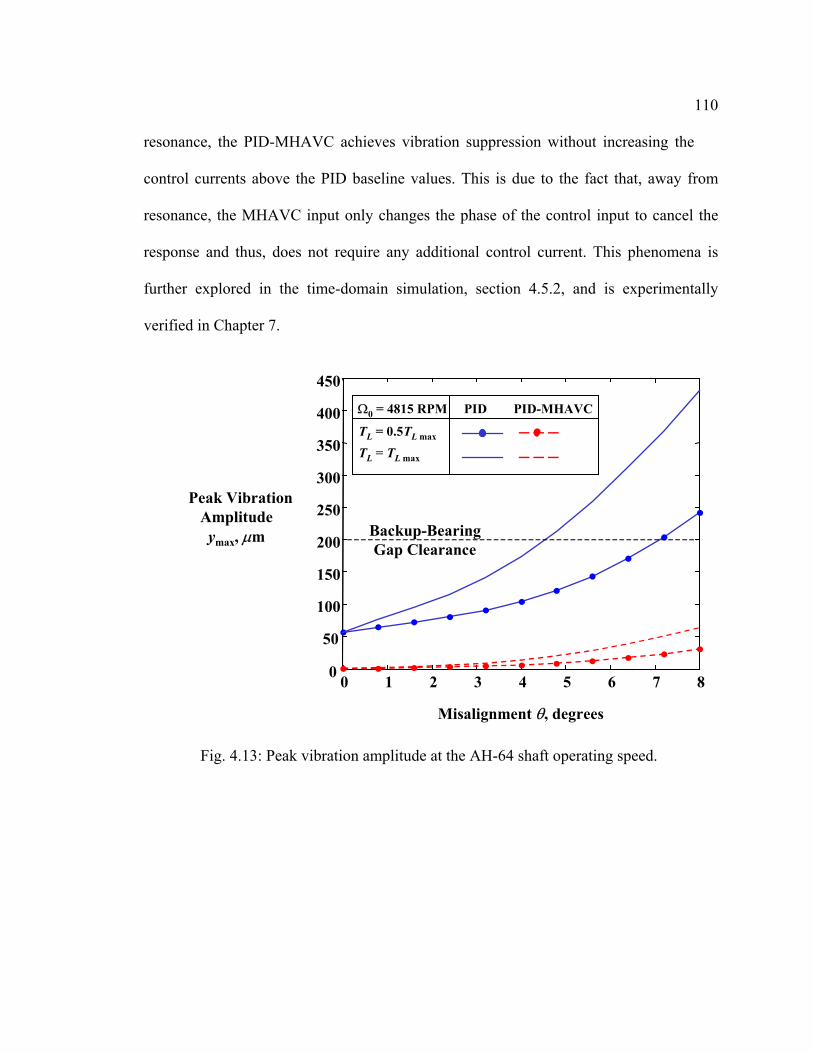
110

resonance, the PID-MHAVC achieves vibration suppression without increasing the

control currents above the PID baseline values. This is due to the fact that, away from

resonance, the MHAVC input only changes the phase of the control input to cancel the

response and thus, does not require any additional control current. This phenomena is

further explored in the time-domain simulation, section 4.5.2, and is experimentally

verified in Chapter 7.

0 1 2 3 4 5 6 7 80

50

100

150

200

250

300

350

400

450


Misalignment θ, degrees

TL = 0.5TL max

TL = TL max

Ω0 = 4815 RPM PID PID-MHAVC

Peak VibrationAmplitudeymax, µm

Fig. 4.13: Peak vibration amplitude at the AH-64 shaft operating speed.

111

4.5.2 Time-Domain Simulation

This section describes the signal-processing required to implement the PID-

MHAVC control law and investigates the time-domain response of the PID-MHAVC

controlled AMB-NCV-driveline system. The closed-loop system is implemented and

simulated under Matlab Simulink. The block diagram of the overall system is given by

Figure 4.15.

TL = 0.5TL max

TL = TL max

Ω0 = 4815 RPM PID PID-MHAVC

0 1 2 3 4 5 6 7 80

0.5

1

1.5

2

2.5

3

3.5

4

Misalignment θ, degrees

Bias Current Peak ControlCurrent

imax, Amps

Fig. 4.14: Peak AMB control current at the AH-64 shaft operating speed.

112

The MHAVC is implemented with 3 sub-blocks. The first sub-block, is the de-

convolving Harmonic Fourier Coefficient (HFC) calculator, shown in Figure 4.16.

MHAVCSynthesis

iY

Multi-Harmonic AdaptiveVibration Control

1+iU

PID Controlled AMB-Driveline

0Ω

z

y

d

LT θ

uMHAVC

xCz

xCytuBtdBxtAxtE

z

y

MHAVCud

=

=++= )()()()( &

0Ω]ˆ[ˆ]ˆˆ[ 1

1 iiyuT

yuyuT

yui YUTWTTWTU −= −+

HFCCalculator

Fig. 4.15: PID-MHAVC controlled AMB-driveline system.

iY )(ty2

Multi-ChannelMoving AverageLow-Pass Filter

M

)sin( 0 skTΩ

)cos( 0 skTΩ

)sin( 0 sh kTn Ω

)cos( 0 sh kTn Ω

MU

X

Tupdate Ts

HFC Calculator

Fig. 4.16: Real-time Harmonic Fourier Coefficient calculator block.

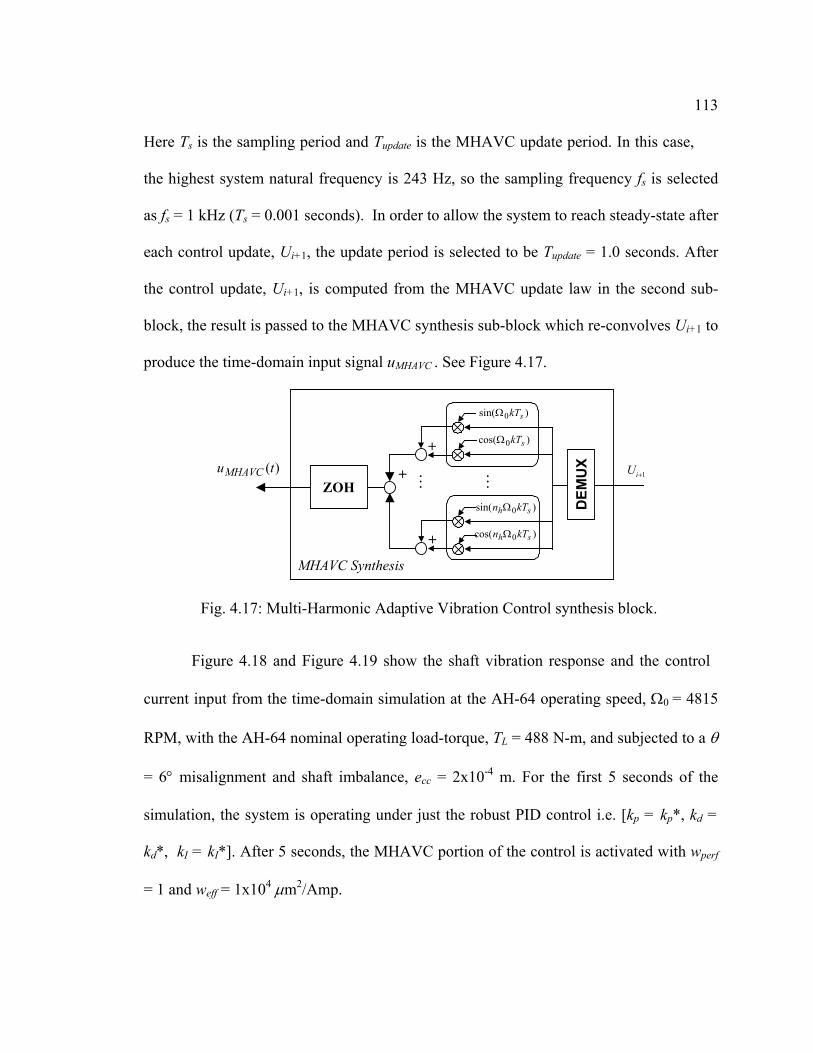
113

Here Ts is the sampling period and Tupdate is the MHAVC update period. In this case,

the highest system natural frequency is 243 Hz, so the sampling frequency fs is selected

as fs = 1 kHz (Ts = 0.001 seconds). In order to allow the system to reach steady-state after

each control update, Ui+1, the update period is selected to be Tupdate = 1.0 seconds. After

the control update, Ui+1, is computed from the MHAVC update law in the second sub-

block, the result is passed to the MHAVC synthesis sub-block which re-convolves Ui+1 to

produce the time-domain input signal uMHAVC . See Figure 4.17.

Figure 4.18 and Figure 4.19 show the shaft vibration response and the control

current input from the time-domain simulation at the AH-64 operating speed, Ω0 = 4815

RPM, with the AH-64 nominal operating load-torque, TL = 488 N-m, and subjected to a θ

= 6° misalignment and shaft imbalance, ecc = 2x10-4 m. For the first 5 seconds of the

simulation, the system is operating under just the robust PID control i.e. [kp = kp*, kd =

kd*, kI = kI*]. After 5 seconds, the MHAVC portion of the control is activated with wperf

= 1 and weff = 1x104 µm2/Amp.

1+iUM

+

+

+

M

DEM

UX

)sin( 0 skTΩ

)cos( 0 skTΩ

)sin( 0 sh kTn Ω

)cos( 0 sh kTn Ω

ZOH)(tuMHAVC

MHAVC Synthesis

Fig. 4.17: Multi-Harmonic Adaptive Vibration Control synthesis block.

114

The time domain simulations confirm the stability and convergence

robustness of the design and also validates the design methodology. In particular, it

confirms the validity of using of the truncated harmonic balance method to approximate

the multi-harmonic transfer matrix Tyu (4.19) of the LPTV driveline system in the

convergence analysis (4.31).

Also, the simulation shows the performance robustness of the PID-MHAVC

controlled system with respect to the misalignment and load torque NCV effect as well as

imbalance. This is the case, since, the control is able to suppress the multi-frequency

driveline vibration without knowledge of the imbalance, misalignment or load torque

operating conditions.

0 5 10 15 20 25 30-100-50

050

100

0 5 10 15 20 25 30-100-50

050

100

0 5 10 15 20 25 30-100-50

050

100

0 5 10 15 20 25 30-100-50

050

100

0 5 10 15 20 25 30-100-50

050

100

0 5 10 15 20 25 30-100-50

050

100

time, sec

v-di

r di

sp.

AM

B3,

µm

v-di

r di

sp.

AM

B2,

µm

v-di

r di

sp.

AM

B1,

µm

w-d

ir d

isp.

AM

B3,

µm

w-d

ir d

isp.

AM

B2,

µm

w-d

ir d

isp.

AM

B1,

µm

PID-MHAVC

Activate MHAVC

PID

Fig. 4.18: PID-MHAVC controlled AMB-driveline shaft vibration response.

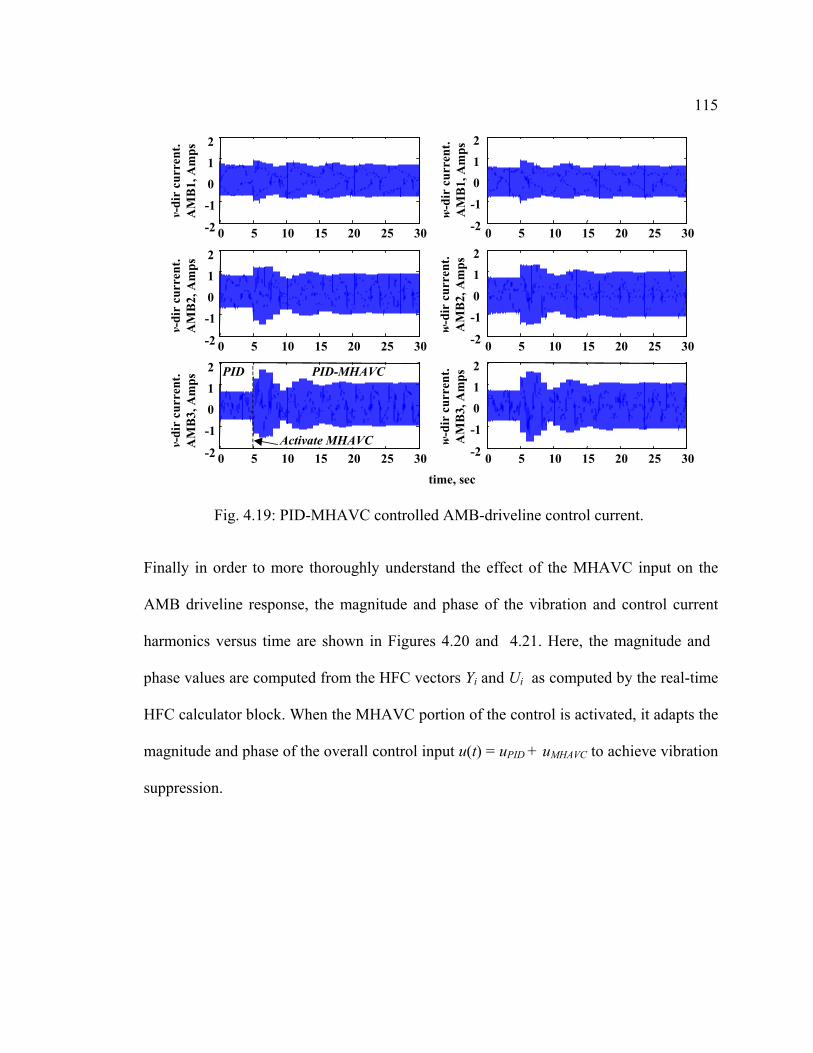
115

Finally in order to more thoroughly understand the effect of the MHAVC input on the

AMB driveline response, the magnitude and phase of the vibration and control current

harmonics versus time are shown in Figures 4.20 and 4.21. Here, the magnitude and

phase values are computed from the HFC vectors Yi and Ui as computed by the real-time

HFC calculator block. When the MHAVC portion of the control is activated, it adapts the

magnitude and phase of the overall control input u(t) = uPID + uMHAVC to achieve vibration

suppression.

time, sec

0 5 10 15 20 25 30-2

-1

0

1

2

0 5 10 15 20 25 30-2

-1

0

1

2

0 5 10 15 20 25 30-2

-1

0

1

2

w-d

ir c

urre

nt.

AM

B3,

Am

psw

-dir

cur

rent

.A

MB

2, A

mps

w-d

ir c

urre

nt.

AM

B1,

Am

ps

0 5 10 15 20 25 30

0 5 10 15 20 25 30

0 5 10 15 20 25 30

-2

-1

0

1

2

-2

-1

0

1

2

-2

-1

0

1

2

v-di

r cu

rren

t.A

MB

3, A

mps

v-di

r cu

rren

t.A

MB

2, A

mps

v-di

r cu

rren

t.A

MB

1, A

mps

PID-MHAVC

Activate MHAVC

PID

Fig. 4.19: PID-MHAVC controlled AMB-driveline control current.

116

0 10 20 300

50

100

0 10 20 300

10

20

0 10 20 300

1

2

0 10 20 300

5

10

0 10 20 30-200

0

200

0 10 20 30-200

0

200

0 10 20 30-200

0

200

0 10 20 30-200

0

200

time, sec


4Ω0 Harmonic

3Ω0 Harmonic

2Ω0 Harmonic

Vib

ratio

n M

agni

tude

, µm

Vib

ratio

n Ph

ase

Ang

le, D

egre

esActivate MHAVC

Fig. 4.20: Shaft vibration magnitude and phase at AMB1.

0 10 20 30

0 10 20 30

0 10 20 30

0 10 20 30

0.4

0.6

0.8

0.1

0.15

0.2

0

0.05

0.1

0

0.2

0.4

0 10 20 30

0 10 20 30

0 10 20 30

0 10 20 30

-200

-150

-100

0

100

200

0

100

200

-200

0

200

time, sec

Con

trol

Cur

rent

Mag

nitu

de, A

mps

Con

trol

Cur

rent

Pha

se A

ngle

, Am

ps


4Ω0 Harmonic

3Ω0 Harmonic

2Ω0 Harmonic

Activate MHAVC

Fig. 4.21: Control current magnitude and phase at AMB1.

117

4.6 Configuration I Control Law Summary and Conclusions

While previous research, together with the new findings in Chapter 3, have found

that NCV couplings greatly impact driveline stability and cause significant multi-

harmonic excitation, this issue has yet to be addressed in the context of active magnetic

bearing control of driveshafts. Due to the nature of the NCV terms, traditional robust

control strategies, such as H∞, µ-synthesis, and Sliding Mode control, are not adequate to

guarantee both robust stability and robust vibration suppression performance.

Specifically, the H∞ control approach, Zhou, et al. (1996), is inadequate because it does

not account for the structure of the uncertain NCV terms in the control synthesis. Since

the NCV driveline system has multiple uncertain parameters, not accounting for the

uncertainty structure could lead to unnecessary conservatism in the control design

resulting in poor closed-loop vibration performance. Furthermore, since the uncertainty is

time-varying, µ-synthesis techniques, Nonami and Takayuki (1996), cannot be utilized.

Finally, robust Sliding Mode control techniques, Utkin (1977) and Sinha and Miller

(1995), cannot be effectively utilized since the NCV terms do not satisfy a matching

condition.

To overcome these challenges, this chapter develops a robust-adaptive active

control law based on a hybrid PID feedback/Multi-Harmonic Adaptive Vibration Control

(PID-MHAVC) approach. This control strategy effectively suppresses both the

synchronous imbalance vibration and the super-synchronous vibrations induced by

misalignment and load-torque NCV effects in AMB-driveline systems.

118

Advancing from the open-loop SAVC developed for LTIV systems in

Knospe, et al. (1993), a multi-harmonic version (MHAVC) is developed for an AMB-

NCV driveline (an LPTV system). By utilizing a harmonic balance approach, a multi-

harmonic Fourier coefficient transfer matrix representation, Tyu, is determined for the

AMB-NCV driveline system. This representation enables the MHAVC update law to be

formulated based on least-squares minimization of an objective function and allows a

convergence robustness analysis to be developed.

Using these results, the robust PID-MHAVC controller was designed for an

AMB-NCV driveline based on an AH-64 helicopter tailrotor driveline system. In the

control design, the shaft imbalance, ecc, and the operating conditions, Ω0, TL and θ, were

considered to be uncertain within a given range and thus the periodic NCV terms were

treated as modeling uncertainty. Robust BIBO stability was ensured by designing the PID

feedback control gains and robust convergence of the MHAVC input was ensured by

adjusting a control effort weighting parameter in the MHAVC objective function.

Finally, the performance of the PID-MHAVC controlled AMB driveline system is

analyzed over a range of operating conditions. The results of the performance analysis

show that the PID-MHAVC control effectively suppresses the multi-harmonic vibration

due to shaft imbalance and the NCV effects. Since good attenuation is achieved without

using explicit knowledge of the misalignment, load-torque or imbalance, the control is

deemed to have robust performance. Additionally, since the required control currents are

on the order of the AMB bias currents, the PID-MHAVC law developed in this chapter is

119

feasible for the AH-64 tailrotor driveline application with the current magnetic

bearings considered in this investigation.

120

Chapter 5

CONFIGURATION II: ROBUST ADAPTIVE VIBRATION CONTROL OF

FLEXIBLE MATRIX COMPOSITE DRIVELINES VIA MAGNETIC BEARINGS

5.1 Introduction

Recently, a novel approach to the design of helicopter tailrotor drivelines based

on newly emerging Flexible Matrix Composite (FMC) materials has been explored by,

Shan and Bakis (2002), Shan and Bakis (2003), Ocalan (2002) and Shin, et al. (2003). It

has been found that shafts constructed of such FMC materials can provide many benefits

over conventional segmented metal alloy driveshafts. In particular, Shin, et al. (2003)

found that, by proper tailoring of the FMC ply thickness and fiber orientations, FMC

tailrotor driveshaft designs with high torsion stiffness and low lateral-bending stiffness

can be achieved with less-weight than conventional alloy shaft designs. Due to the high

strain capability of FMC materials, see Shan and Bakis (2002), it was demonstrated by

Ocalan (2002) and Shin, et al. (2003) that such FMC shaft designs can safely

accommodate tailrotor driveline angular misalignments and eliminate the need for

121

flexible couplings, which are a significant source of driveline vibration and

maintenance requirements.

Despite these benefits, FMC shafts have been found to have significantly more

structural damping compared with conventional alloy or rigid matrix composite shafts,

Shan and Bakis (2002). Consequently, FMC shafts are more prone to both self-heating,

and rotating-frame damping induced whirl instability, Shin, et al. (2003). Furthermore,

another challenge posed by FMC shafts is the temperature sensitivity of the FMC

material properties. In Shan and Bakis (2003), it was demonstrated that the FMC ply

elastic moduli and damping loss-factors were temperature dependent. The temperature

sensitivity poses several challenges for the design of stable, low vibration FMC tailrotor

driveline systems. In particular, the stiffness and damping temperature sensitivity

together with the stiffness and damping dependent self-heating, could allow for coupled

temperature/vibration dynamics which has the potential to cause limit-cycle oscillations

or instability. Furthermore, the stiffness variation due to ambient temperature fluctuations

could also lead to instability or high vibration levels by shifting the system natural

frequencies close to or below the driveline operating speed.

To address these issues and advance the state-of-the-art, the objective of this

chapter is to explore the use of non-contact Active Magnetic Bearings (AMB) technology

together with active vibration control techniques in order to guarantee stable, low

vibration operation of a single piece FMC tailrotor driveline. In this chapter, a robust-

adaptive vibration control strategy based on a hybrid H∞/SAVC approach is developed

122

which accounts for the main source of vibration (shaft imbalance) and uncertainty

(temperature dependent stiffness and damping) in FMC driveline systems.

5.2 AMB-FMC Driveline System

Figure 5.1 depicts the AMB-FMC flexible driveline system investigated in this

research. The system consists of a single piece FMC shaft, length Ls, which is driven at

constant rotational speed, Ω. The shaft is coupled to a fixed input-shaft and fixed output-

shaft via rigid couplings and is supported by three radial AMBs at locations Lamb1, Lamb2

and Lamb3. Here, v(x,t) and w(x,t) are the transverse shaft deflections.

FMC DriveshaftRigid

Coupling Ω

Lamb2

RigidCoupling

AMB1 AMB2

Lamb1

Lamb3

AMB3

Ls

Shaft Temperature. T

),( & ),( txwtxv

Fig. 5.1: Configuration II: one-piece FMC driveline with AMBs and rigid couplings.

123

Unlike the driveline configurations explored in the previous chapters, which have

flexible couplings with NCV kinematics, the current FMC driveline system has rigid

couplings with constant velocity kinematics. Thus, misalignment and load-torque do not

explicitly affect the driveline dynamics or stability since the NCV terms are zero.

The FMC shaft considered in this investigation is composed of 4 ply layers which

are assembled in symmetric layup configuration. The ply orientations are described as

[+θ1/-θ1/-θ2/+θ2], where θ1 and θ2 are the fiber-orientation angles relative the shaft axis.

Based on the layup angles and the ply material properties, the equivalent isotropic elastic

and shear moduli, E and G, of the assembled FMC shaft are obtained using Classical

Lamination Theory, Jones (1975). See Appendix F. Since the FMC material properties

are temperature dependent, the equivalent isotropic shaft material parameters are

E = E(T), G = G(T) and ξ = ξ(T) ( 5.1 )

Where E and G are elastic and shear moduli, ξ is an equivalent viscous damping

parameter and T is the shaft temperature. Also, the nominal shaft material properties are

defined as

En = E(Tn), Gn = G(Tn) and ξn = ξ(Tn) ( 5.2 )

with nominal temperature, Tn = 85°F. Finally, the shaft material property temperature

dependence is linearly approximated about the nominal values as

( ) ( )( ) 1)()(

1)( , 1)(

nncT

nTnkT

ETETGTGETE

ξδδξδδδδ τ

+≈+≈+≈

( 5.3 )

Where δk, δτ, and δc, are bending stiffness, torsion stiffness and damping temperature

sensitivities and δT = T - Tn is the driveline deviation temperature about Tn due to the

124

ambient temperature operating conditions. See Tables 5.1 and 5.2 for the FMC shaft

material properties considered in this investigation.

The AMBs are modeled based on the linearized force-current-displacement relations

about some bias current level, ibias. The AMB-FMC driveline equations-of-motion are

obtained via Finite Element Method (FEM) and the model order is reduced by

Table 5.1: FMC Material Properties and Ply Configuration

FMC Ply Material Properties a

Density, ρs 1650 kg/m3

Longitudinal modulus, El 115 GPaTransverse modulus, Et 0.275 GPaShear modulus, Glt 0.250 GPaLongitudinal loss-factor, ηl 0.0011Transverse loss-factor, ηt 0.080Shear loss-factor, ηtl 0.085Poisson’s Ratio, νtl 0.38FMC Shaft Ply ConfigurationNumber of ply layers, nl 4Ply layer thickness, tl 0.772 mmFiber orientations, θi [+45°/-45°/-90°/+90°]

a All values at nominal temperature, Tn = 85°F, Shan and Bakis (2003)

Table 5.2: Equivalent Isotropic Properties

FMC Shaft Equivalent Isotropic PropertiesDensity, ρs 1650 kg/m3

Elastic modulus (nominal), En 11.84 GPaShear modulus (nominal), Gn 14.51 GPaEquivalent viscous damping a, ξn 5.85 x10-5

Temperature Sensitivity ParametersBending stiffness sensitivity, δk -0.0625 % / °FTorsion stiffness sensitivity, δτ -2.0x10-3 % / °FDamping sensitivity, δc 0.125 % / °F

a Viscous damping based on loss-factor at 10 Hz

125

performing a truncated modal transformation retaining the first ten (Nmode = 10)

undamped, non-gyroscopic, mass-normalized modes. The resulting equations-of-motion

in terms of the truncated modal coordinate vector 1mode)( ×ℜ∈ Ntη is

[ ] [ ]

[ ] )(cossin

)()1()1( )()1(

tutt T

cTkTcT

AMBIMB

AMBrd

QQ

KKKGCM

+ΩΩ=

+Ω++++Ω+++

L

&&& ηδδδδηδδη( 5.4 )

Where “ . ” indicates time differentiation and the matrices M, C, G and K are the

nominal inertia, structural damping, gyroscopic and elastic stiffness matrices with M = I

(identity matrix). Krd is the skew-symmetric rotating-frame damping-stiffness matrix,

Zorzi and Nelson (1977), and KAMB, is the negative AMB stiffness matrix for the bias

current level ibias. Finally, 2mode×ℜ∈ NIMBQ describes the synchronous shaft imbalance

excitation and unN ×ℜ∈ modeAMBQ is the AMB force-current input distribution matrix, with

control current input vector 1 )( ×ℜ∈ untu .

In this investigation, the AMB-FMC driveline is sized to replace the conventional

segmented tailrotor driveline of the Boeing AH-64 Apache helicopter. In particular, the

overall driveline length, Ls, and the shaft outer diameter, Ds, is kept the same as the

original AH-64 driveline. Furthermore, the FMC shaft wall thickness, ts, is selected such

that the torsion stiffness of FMC driveline also matches that of the original AH-64

driveline. Tables 5.3 and 5.4 summarize the driveline and AMB parameters considered

in this analysis. Here, the AMBs are the same design as the ones utilized in Configuration

I (Chapter 4). However, due to the lower bending stiffness of the FMC shaft, a lower bias

current setting, ibias = 1.5 Amps, is selected compared with , ibias = 2.5 Amps, in the alloy

shaft case.

126

5.3 Active Control Structure

To proceed with development of the active control, the AMB-FMC driveline

system (5.4) is first recast into state-space form

Table 5.3: FMC Driveline Parameters

Shaft DimensionsOuter Diameter, DsWall thickness, tsLength, LsNumber of segments, nseg

0.1143 m3.089 mm6.667 m1

Magnetic Bearing LocationsLocation of AMB1, Lamb1Location of AMB2, Lamb2Location of AMB3, Lamb3

0.2 Ls =1.33 m0.5 Ls =3.66 m0.8 Ls =5.34 m

Operating ConditionsOperating Speed, Ω 4815 RPMShaft eccentricity, ecc 5.0x10-5 mImbalance location, Limb 0.3 Ls = 2.0 m

Table 5.4: AMB Parameters

AMB Properties

Rotor-stator gap, hgap 500 µmBackup-bearing gap, hback 200 µmSaturation current, isat 5.3 AmpsBias current, ibias 1.5 AmpsForce constant, Gb 9.1x10-6 N m2/Amp2

Peak force capacity, Fmax 445 NRMS force capacity, Frms 311 NControl axis angle, θb 45°Coil-Sensor offset, dsens 25.4 mmAMB rotor length, Lrotor 37.5 mmAMB rotor mass, mrotor 0.645 kg

127

[ ]

xCyxCz

tuBtdBxAAx

y

z

udTTn

==

+++= )()(δ&

( 5.5 )

With state vector 1][ ×ℜ∈= xnTTx ηη & , the nominal system matrix, An, and deviation

temperature-induced perturbation matrix, AT, are written as

( ) ( )

−+−

=

+−++−

=CKKGCKKK

I

rdAMBrd cckTn AA

δδδ )(00

0

( 5.6 )

Also, Ttttd ]cossin[)( ΩΩ= is the synchronous disturbance input due to imbalance and

1 ×ℜ∈ unu is the AMB control input with corresponding input distribution matrices

dnxndB ×ℜ∈ and unxn

uB ×ℜ∈ written as

=

IMBQ0

dB and

=

AMBQ0

uB ( 5.7 )

Additionally 1 ×ℜ∈ yny is the output vector of shaft displacements measured by the AMB

sensors and 1 ×ℜ∈ znz is the performance output vector. Each of the three AMBs has two

independent control axes and two corresponding displacement sensors, thus nu = ny = 6.

Figure 5.2 is a block diagram of the closed-loop AMB-FMC driveline system.

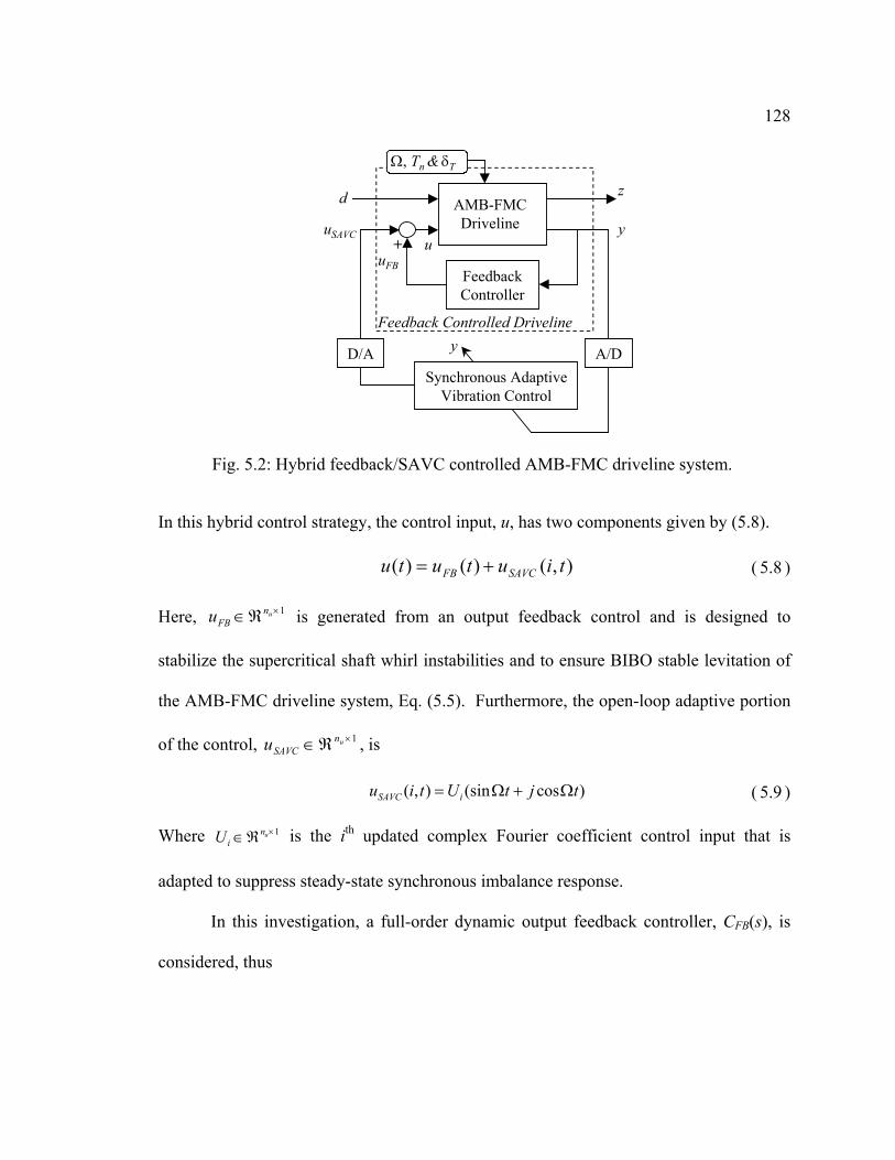
128

In this hybrid control strategy, the control input, u, has two components given by (5.8).

),()()( tiututu SAVCFB += ( 5.8 )

Here, 1 ×ℜ∈ unFBu is generated from an output feedback control and is designed to

stabilize the supercritical shaft whirl instabilities and to ensure BIBO stable levitation of

the AMB-FMC driveline system, Eq. (5.5). Furthermore, the open-loop adaptive portion

of the control, 1 ×ℜ∈ unSAVCu , is

)cos(sin),( tjtUtiu iSAVC Ω+Ω= ( 5.9 )

Where 1 ×ℜ∈ uniU is the ith updated complex Fourier coefficient control input that is

adapted to suppress steady-state synchronous imbalance response.

In this investigation, a full-order dynamic output feedback controller, CFB(s), is

considered, thus

FeedbackController

+

Feedback Controlled Driveline

AMB-FMCDriveline

Synchronous AdaptiveVibration Control

A/DD/A

z

yu

uFB

d

uSAVC

Ω, Tn & δT

y

Fig. 5.2: Hybrid feedback/SAVC controlled AMB-FMC driveline system.

129

+=+=

=yDxCu

yBxAxsC

cccFB

ccccFB

&:)( (5.10)

Where 1 ×ℜ∈ cncx is the controller state and nc = nx is the controller order. In this case,

since the first 10 modes are considered, nx = 20. From (5.5) and (5.10), the feedback

controlled driveline system is

clycl

clzcl

SAVCucldclclclcl

xCyxCz

tuBtdBxAx

==

++= )()(&

(5.11)

with augmented state vector TTc

Tcl xxx ][= and

0

,0

]0[

]0[

000

,

=

=

=

=

=

+=

+=

uucl

ddcl

zzcl

yycl

TclT

cyc

cuycunncl

clTTnclcl

BB

BB

CC

CC

AA

ACBCBCDBA

A

AAA δ

(5.12)

Assuming the feedback controlled AMB-FMC driveline system in (5.11) is BIBO stable,

the steady-state response after the ith SAVC control input, Ui, is

FBiyui YUTY += (5.13)

Where Tyu is the synchronous transfer matrix from the control input to the measured

output 5.14

[ ] uclclyclyu BAIjCT 1−−Ω= (5.14)

and DTY ydFB = is the steady-state imbalance response of the feedback controlled driveline

system without SAVC input.

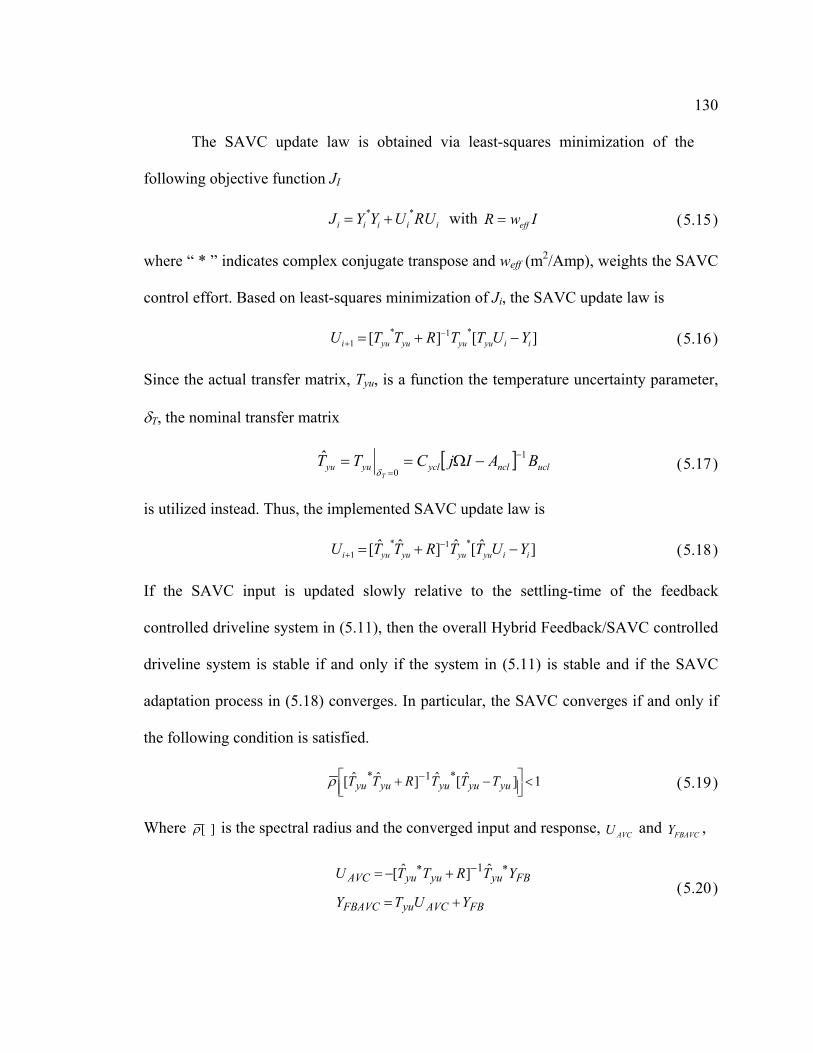
130

The SAVC update law is obtained via least-squares minimization of the

following objective function JI

iiiii RUUYYJ ** += with IwR eff= (5.15)

where “ * ” indicates complex conjugate transpose and weff (m2/Amp), weights the SAVC

control effort. Based on least-squares minimization of Ji, the SAVC update law is

][][ *1*1 iiyuyuyuyui YUTTRTTU −+= −+ (5.16)

Since the actual transfer matrix, Tyu, is a function the temperature uncertainty parameter,

δT, the nominal transfer matrix

[ ] uclnclyclyuyu BAIjCTTT

1

0ˆ −

=−Ω==

δ(5.17)

is utilized instead. Thus, the implemented SAVC update law is

]ˆ[ˆ]ˆˆ[ *1*1 iiyuyuyuyui YUTTRTTU −+= −+ (5.18)

If the SAVC input is updated slowly relative to the settling-time of the feedback

controlled driveline system in (5.11), then the overall Hybrid Feedback/SAVC controlled

driveline system is stable if and only if the system in (5.11) is stable and if the SAVC

adaptation process in (5.18) converges. In particular, the SAVC converges if and only if

the following condition is satisfied.

1]ˆ[ˆ]ˆˆ[ *1* <

−+ −

yuyuyuyuyu TTTRTTρ (5.19)

Where ] [ρ is the spectral radius and the converged input and response, AVCU and FBAVCY ,

FBAVCyuFBAVC

FByuyuyuAVC

YUTY

YTRTTU

+=

+−= ∗−∗ ˆ]ˆ[ 1

(5.20)

131

Since errors between the actual transfer matrix, yuT , and the nominal transfer matrix,

yuT , could cause the SAVC input not to converge, the convergence robustness must be

considered in the control design.

5.4 Control Synthesis

Conceptually, in the hybrid Feedback-SAVC control system, the function of the

feedback control in (5.10) is to ensure BIBO stable levitation of the AMB-FMC-driveline

while the SAVC adapts and converges to suppress the steady-state imbalance vibration.

Since the slowly adapted SAVC input does not affect BIBO stability, the feedback

controller and the SAVC design and analyses can be conducted sequentially.

Since the control system must be robust with respect to temperature deviations,

δT, about the nominal temperature, δT is considered as a bounded uncertainty parameter in

the control design. Thus, the feedback controlled AMB-FMC driveline system is

rewritten as a linear fractional transformation (LFT) about the nominal feedback

controlled system, G(s), with deviation temperature uncertainty block ∆ = δTI.

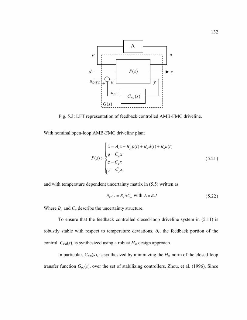
132

With nominal open-loop AMB-FMC driveline plant

==

=

+++=

=

xCyxCz

xCqtuBtdBtpBxAx

sP

y

z

q

udpn )()()(

:)(

&

(5.21)

and with temperature dependent uncertainty matrix in (5.5) written as

qpTT CBA ∆=δ with ITδ=∆ (5.22)

Where Bp and Cq describe the uncertainty structure.

To ensure that the feedback controlled closed-loop driveline system in (5.11) is

robustly stable with respect to temperature deviations, δT, the feedback portion of the

control, CFB(s), is synthesized using a robust H∞ design approach.

In particular, CFB(s), is synthesized by minimizing the H∞ norm of the closed-loop

transfer function Gpq(s), over the set of stabilizing controllers, Zhou, et al. (1996). Since

uSAVC

)(sP

p

d

uFB

y

z

q

)(sCFB

u+

)(sG

∆

Fig. 5.3: LFT representation of feedback controlled AMB-FMC driveline.

133

Tδ=∆∞

, when γ<∞

)(sGqp , BIBO stability of the feedback controlled driveline

system is guaranteed for all bounded temperatures deviations satisfying

γδδ /1stab =≤ TT (5.23)

where δTstab is the deviation temperature robust stability margin.

In this investigation, the H∞ feedback controller is computed using the

MATLAB LMI Control Toolbox software package. For the AMB-FMC driveline

system studied in this research, a feedback controller, CFB(s), which achieves γ = 0.0034

(δTstab = 294°F) is synthesized. Since δTstab = 294°F is well above the expected shaft

temperature deviations, this is considered a robust design and is utilized for the feedback

portion of the hybrid feedback/SAVC law in the subsequent analysis.

To analyze the convergence robustness of the SAVC portion of the control, the

convergence criteria in (5.19) is iteratively solved using a bisection algorithm to

determine the deviation temperature robust convergence margin, δTconv, for a range of

shaft speeds. Finally, the overall deviation temperature robustness margin δTmax for a

given shaft speed, Ω, is defined and computed as

δTmax = min[δTstab , δTconv] (5.24)

To asses the vibration performance, the following worst-case steady-state vibration

indices are defined for a given deviation temperature bound, ∆T

=

∆≤≤FBFB

yTTFB YY

nJ *

0

1supδ

,

=

∆≤≤FBAVCFBAVC

yTTFBAVC YY

nJ *

0

1sup δ

(5.25)

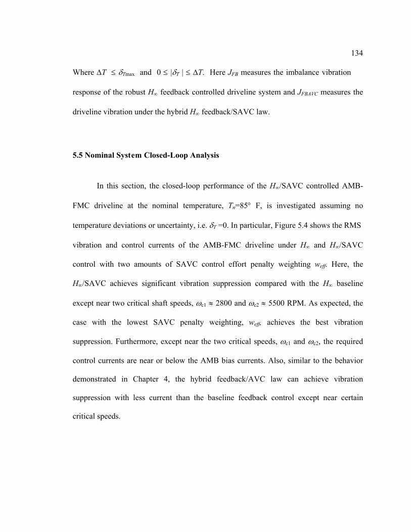
134

Where ∆T ≤ δTmax and 0 ≤ |δT | ≤ ∆T. Here JFB measures the imbalance vibration

response of the robust H∞ feedback controlled driveline system and JFBAVC measures the

driveline vibration under the hybrid H∞ feedback/SAVC law.

5.5 Nominal System Closed-Loop Analysis

In this section, the closed-loop performance of the H∞/SAVC controlled AMB-

FMC driveline at the nominal temperature, Tn=85° F, is investigated assuming no

temperature deviations or uncertainty, i.e. δT =0. In particular, Figure 5.4 shows the RMS

vibration and control currents of the AMB-FMC driveline under H∞ and H∞/SAVC

control with two amounts of SAVC control effort penalty weighting weff. Here, the

H∞/SAVC achieves significant vibration suppression compared with the H∞ baseline

except near two critical shaft speeds, ωc1 ≈ 2800 and ωc2 ≈ 5500 RPM. As expected, the

case with the lowest SAVC penalty weighting, weff, achieves the best vibration

suppression. Furthermore, except near the two critical speeds, ωc1 and ωc2, the required

control currents are near or below the AMB bias currents. Also, similar to the behavior

demonstrated in Chapter 4, the hybrid feedback/AVC law can achieve vibration

suppression with less current than the baseline feedback control except near certain

critical speeds.

135

Near the operating speeds, ωc1 and ωc2, the SAVC requires excessive currents to

suppress the vibration and thus, due to AMB current saturation limitations, the imbalance

vibration cannot as effectively be reduced at these speeds. Physically, this phenomena is

due to transmission zeros in the control path which are introduced by the H∞ feedback

controller CFB(s). See Figure 5.3. The control path zeros attenuate the effectiveness of

the SAVC portion of the control at frequencies corresponding to the imaginary part of the

transmission zeros. This phenomena was not encountered with the PID-MHAVC law

developed in Chapter 4 since the PID feedback does not introduce any transmission zeros

or any internal model dynamics.

0 1000 2000 3000 4000 5000 60000

50

100

150

200

250R

MS

Shaf

t Vib

ratio

n, µ

mBackup-BearingGap Clearance

Shaft Speed Ω, RPM

RM

S C

ontr

ol C

urre

nt, A

mps

0 1000 2000 3000 4000 5000 60000

1

2

3

4

Bias Current

H∞

H∞ / SAVC, weff = 5.0x10-7

Controller Settings

H∞ / SAVC, weff = 1.0x10-9

1cω

2cω

1cω

2cω

Fig. 5.4: RMS vibration and control currents vs. shaft speed, system at Tn=85°.

136

The effect of the transmission-zero critical speeds is not necessarily a serous

issue, since most drivelines, such as helicopter drivelines, typically operate at a single

speed Ω. Thus, unless Ω corresponds with one of the transmission-zero speeds, the

hybrid H∞/SAVC law can be used to achieve effective vibration suppression. However,

one way to address this issue is through proper selection of the AMB locations along the

driveline. It is found that the transmission zeros are very sensitive to the AMB locations,

and thus the transmission-zero critical speeds can be shifted away from a given operating

speed by proper AMB placement. This is demonstrated in Figure 5.5, where the

H∞/SAVC controlled AMB-FMC driveline RMS vibration and control currents for two

sets of AMB locations are shown.

AMB Locations[Lamb1=0.2Ls, Lamb2=0.5Ls, Lamb3=0.8Ls]

[Lamb1=0.3Ls, Lamb2=0.5Ls, Lamb3=0.7Ls]

0 1000 2000 3000 4000 5000 60000

50

100

150

200

250

RM

S Sh

aft V

ibra

tion,

µm


Shaft Speed Ω, RPM

0 1000 2000 3000 4000 5000 60000

1

2

3

4

RM

S C

ontr

ol C

urre

nt, A

mps

Bias Current

1cω

2cω

2cω′1cω′

1cω2cω

2cω′1cω′

Controller SettingH∞ / SAVC, weff = 1.0x10-9

Fig. 5.5: Effect of AMB location on transmission-zero critical speeds.

137

5.6 Closed-Loop Analysis with Shaft Temperature Deviations

In this section the effect of temperature uncertainty, δT, is considered. Using

(5.24) and (5.25), the system robustness and imbalance vibration performance is analyzed

over a range of shaft speeds, Ω = [0 - 6000] RPM. This speed range includes both sub

and supercritical operation.

Figure 5.6 shows how δTmax varies with Ω for several values of the SAVC control

effort weighting parameter, weff.

With no SAVC effort penalty (i.e. weff = 0), stability and convergence is

guaranteed for temperature deviations of approximately 100°F about the nominal

temperature, Tn = 85°F, over most of the RPM range. However, for operation speeds near

0 1000 2000 3000 4000 5000 60000

50

100

150

200

250

Shaft Speed, RPM

Rob

ustn

ess M

argi

n δ T

max

, de

gree

s F weff = 0.0weff = 8.0x10-9

weff = 5.5x10-8

weff = 2.0x10-6

ωc1 ωc2

Fig. 5.6: Deviation temperature robustness margin vs. shaft speed for several values of

SAVC control effort penalty weighting, weff .

138

the transmission-zero critical speeds (ωc1 ≈ 2800 and ωc2 ≈ 5500 RPM), the

temperature robustness becomes significantly less. By penalizing the SAVC input (i.e.

selecting weff > 0) the robustness margin near, ωc1 and ωc2, can be increased. In particular,

as seen in Figure 5.6, if weff is chosen to be weff ≥ weff* = 5.5x10-8 m2/Amp, the system

can tolerate temperature deviations up to 100°F and still remain stable and converge

across the examined RPM range. That is, weff = weff

* = 5.5x10-8 m2/Amp guarantees δTmax

> 100°F over the speed range Ω = [0 - 6000] RPM.

Considering weff = weff* = 5.5x10-8 m2/Amp to be the lowest acceptable value for

the design, the vibration performance for two values of weff ≥ weff* is examined in Figures

5.7 and 5.8. Note that no knowledge of the shaft imbalance is utilized in the control

synthesis and vibration is suppression is achieved in the presence of the uncertainty δT.

In each plot, the worst-case vibration performance indices, JFB and JFBAVC, are shown for

the nominal system and for a 100°F deviation temperature uncertainty bound. By

comparing the two performance indices, JFB and JFBAVC, and by considering JFB as the

baseline performance, the effectiveness of the SAVC can be assessed.

139

0 1000 2000 3000 4000 5000 60000

50

100

150

200

250

300

Shaft Speed, RPM

Vib

ratio

n In

dice

s, µm

δT = 0[0 ≤ |δT | ≤ 100° F]

JFBAVCJFB

ωc1 ωc2

a

b

c

d

Fig. 5.7: JFB and JFBAVC vs. shaft speed for two levels of temperature uncertainty; [δT

= 0] and [0 ≤ δT ≤ 100°F], with weff 6.0x10-8.

0 1000 2000 3000 4000 5000 60000

50

100

150

200

250

300

Shaft Speed, RPM

Vib

ratio

n In

dice

s, µm

ωc1 ωc2

δT = 0[0 ≤ |δT | ≤ 100° F]

JFBAVCJFB

Fig. 5.8: JFB and JFBAVC vs. shaft speed for two levels of temperature uncertainty; [δT =

0] and [0 ≤ δT ≤ 100°F],, with weff 2.6x10-7.

140

Figure 5.7 demonstrates that, for lower values of control penalty, i.e. for weff near

weff*, the SAVC input adapts and converges to achieve significant imbalance vibration

suppression for operating speeds away from the transmission-zeros critical speeds ωc1

and ωc2. Thus, the hybrid H∞ feedback/SAVC law achieves robust performance for Ω

away from ωc1 and ωc2. However, for speeds near ωc1 and ωc2, the SAVC input is less

effective. In fact, the presence of the uncertainty, δT, causes the SAVC to increase the

vibration above the feedback controlled baseline imbalance response, (see “a” and “b” in

Figure 5.7). Since δ T alters the FMC shaft stiffness and damping, δT shifts the

transmission-zeros critical frequencies, ωc1 and ωc2 about their nominal values. This

frequency shifting is reflected in the plots of the worst-case case performance indices by

the presence of the peaks “a” and “b” about ωc1 and “d” and “c” about ωc2 in Figure 5.7.

The separation bandwidth between “a” and “b” and between “c” and “d” increases with

the deviation temperature uncertainty δT.

Finally, comparing Figures 5.7 and 5.8 demonstrates the effect of increasing weff

on the SAVC vibration suppression performance and robustness. Increasing weff improves

performance robustness for shaft speeds near the critical speeds, ωc1 and ωc2, However,

since increasing weff limits the SAVC control input magnitudes, it reduces the maximum

achievable vibration suppression. Therefore, larger values of weff are only beneficial for

shaft speeds near the transmission-zero critical speeds.

141

5.7 Configuration II Active Control Summary and Conclusions

In this chapter a hybrid H∞ feedback/SAVC control law is developed for the

AMB-FMC tailrotor driveline system (Configuration II) considering effects of

temperature dependent FMC material properties, rotating-frame damping and shaft

imbalance. The hybrid H∞ feedback/SAVC control strategy is conceptually similar to the

hybrid PID-feedback/MHAVC law developed for the AMB-NCV driveline system

(Configuration I) in Chapter 4. In each configuration, the feedback control ensures BIBO

stable levitation of the driveline throughout a range of operating conditions (robust

stability), while the open-loop control inputs (SAVC or MHAVC) are adapted to

suppress the vibrations.

Since the high strain capability of FMC shafting enables driveline misalignment

to be accommodated without flexible couplings, the AMB-FMC driveline configuration

explored in this chapter has several advantages over both the Conventional Configuration

and Configuration I drivelines. Compared with the previous configurations,

Configuration II reduces the number of driveline components by replacing the multi-

segment driveshaft and associated flexible couplings with a single-piece, rigidly coupled,

FMC shaft. By reducing the number of driveline components, the overall driveline

maintenance “turn-around” times could be improved. Furthermore, since rigid couplings

have constant velocity shaft-speed kinematics as opposed to NCV kinematics, replacing

the flexible couplings with rigid couplings has the advantage of directly eliminating the

misalignment and load-torque induced super-synchronous driveline vibrations. As a

result, the primary source of vibration in the AMB-FMC driveline system is only due to

142

the synchronous imbalance excitation. To suppress this vibration, the adaptive portion

of the AMB-FMC driveline control law utilizes a synchronous adaptive vibration control

(SAVC) approach instead of the multi-harmonic adaptive vibration control (MHAVC)

approach required for the Configuration I AMB-NCV driveline in Chapter 4.

Furthermore, unlike Configuration I, the absence of the NCV effects in Configuration II

enables robust H∞ control theory to be utilized in the synthesis of the feedback portion of

the control law. Therefore, the control strategy developed for the AMB-FMC driveline is

a hybrid H∞ feedback/SAVC control.

The results of the investigation and analysis show that the H∞ feedback/SAVC

hybrid control strategy can guarantee stability, convergence and imbalance vibration

suppression of the AMB-FMC driveline under the conditions of bounded shaft

temperature deviations and unknown shaft imbalance. Furthermore, the controller is

effective at both sub and supercritical operating speeds. Specifically, if the weighting on

SAVC effort is low, the control is very effective and robust for suppressing imbalance

vibration at shaft speeds away from closed-loop system transmission-zeros. Additionally,

for shaft speeds operating near the closed-loop system zeros, the temperature robustness

and imbalance vibration suppression performance can be greatly improved by moderately

increasing the SAVC control effort penalty weighting. Finally, by adjusting the AMB

locations, the transmission-zero critical speeds can be effectively shifted to allow low

vibration operation at a particular desired shaft operating speed.

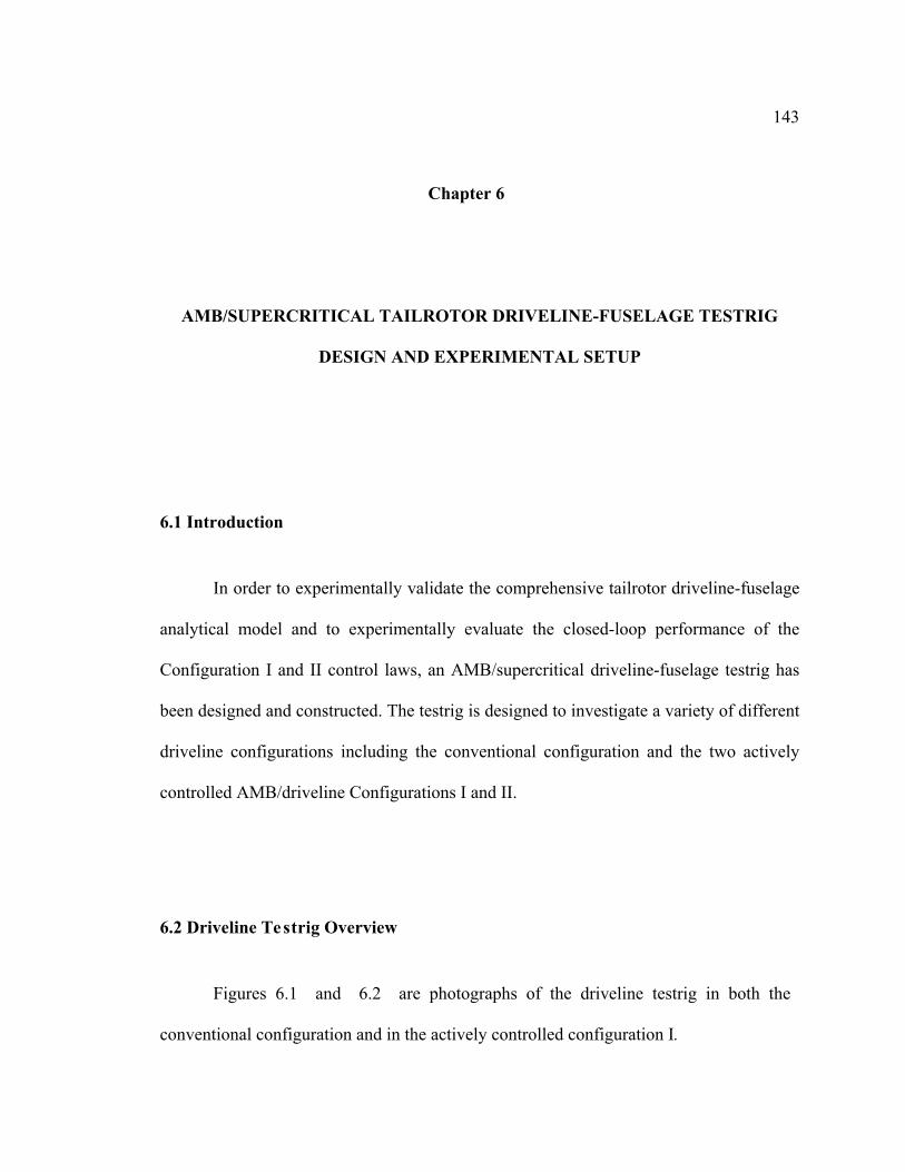
143

Chapter 6

AMB/SUPERCRITICAL TAILROTOR DRIVELINE-FUSELAGE TESTRIG

DESIGN AND EXPERIMENTAL SETUP

6.1 Introduction

In order to experimentally validate the comprehensive tailrotor driveline-fuselage

analytical model and to experimentally evaluate the closed-loop performance of the

Configuration I and II control laws, an AMB/supercritical driveline-fuselage testrig has

been designed and constructed. The testrig is designed to investigate a variety of different

driveline configurations including the conventional configuration and the two actively

controlled AMB/driveline Configurations I and II.

6.2 Driveline Testrig Overview

Figures 6.1 and 6.2 are photographs of the driveline testrig in both the

conventional configuration and in the actively controlled configuration I.

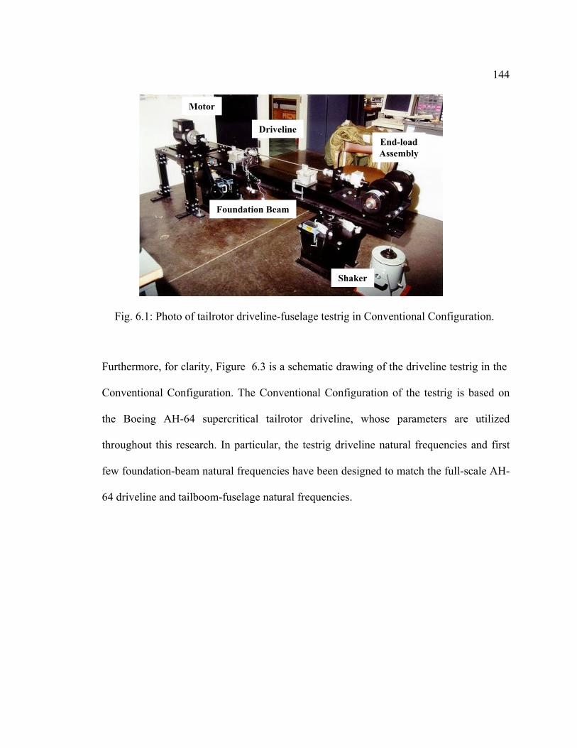
144

Furthermore, for clarity, Figure 6.3 is a schematic drawing of the driveline testrig in the

Conventional Configuration. The Conventional Configuration of the testrig is based on

the Boeing AH-64 supercritical tailrotor driveline, whose parameters are utilized

throughout this research. In particular, the testrig driveline natural frequencies and first

few foundation-beam natural frequencies have been designed to match the full-scale AH-

64 driveline and tailboom-fuselage natural frequencies.

Motor

Shaker

Foundation Beam

DrivelineEnd-loadAssembly

Fig. 6.1: Photo of tailrotor driveline-fuselage testrig in Conventional Configuration.

145

AMB1

AMB2

AMB3

Motor

Load-End

Digital PID Controller(for stabilizingfeedback control)

PC with dSPACE(for adaptive vibrationsuppression)

Fig. 6.2: Photo of tailrotor driveline-fuselage testrig in Configuration I.

1.6 m

Shaker + Imp. headFoundation Beam

Pin Joint

Spring

HangerBearing

Load-EndAssemblyElectric Motor

ViscousDamper

Side-View

Floor

Tri-axis Accelerometer

Fiber-Optic Displacement Probe

Foundation Beam

Top-View

DriveshaftU-joint

CouplingInput-Side Output-Side

A B C

Fig. 6.3: Testrig diagram in Conventional Configuration.

146

The testrig is designed to investigate the driveline vibration and loads under various

foundation excitations, misalignment conditions and torque loads relevant to the real

helicopter tailrotor driveline system.

In the conventional configuration, the testrig main driveshaft (or intermediate

shafts according to Chapter 2) consists of two 32” long shaft segments connected with U-

joint couplings and supported on a flexible foundation beam by a contact roller bearing

and two viscous dampers. The shafts are stainless-steel and have a 3/8” diameter with a

solid circular cross-section.

Figure 6.4 shows the design of the viscous lateral shaft dampers. Here, the lateral

shaft motion is transferred into the two piston-dampers via the grooved non-rotating

bearing-damper ring assembly.

Groove& Slide

Clamp toFoundation

Viscous PistonDampers

Damper-Bearing Ring

Fig. 6.4: Viscous damper assembly for Conventional Configuration, 1 of 2.

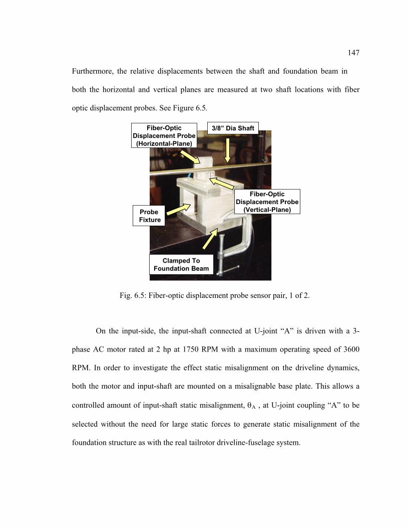
147

Furthermore, the relative displacements between the shaft and foundation beam in

both the horizontal and vertical planes are measured at two shaft locations with fiber

optic displacement probes. See Figure 6.5.

On the input-side, the input-shaft connected at U-joint “A” is driven with a 3-

phase AC motor rated at 2 hp at 1750 RPM with a maximum operating speed of 3600

RPM. In order to investigate the effect static misalignment on the driveline dynamics,

both the motor and input-shaft are mounted on a misalignable base plate. This allows a

controlled amount of input-shaft static misalignment, θA , at U-joint coupling “A” to be

selected without the need for large static forces to generate static misalignment of the

foundation structure as with the real tailrotor driveline-fuselage system.

Clamped ToFoundation Beam

3/8” Dia Shaft

Probe Fixture

Fiber-OpticDisplacement Probe

(Vertical-Plane)

Fiber-OpticDisplacement Probe(Horizontal-Plane)

Fig. 6.5: Fiber-optic displacement probe sensor pair, 1 of 2.

148

On the output-side, connected at U-joint “C”, the driveline drives the end-load

assembly, shown in Figure 6.6, whose main function is to simulate the effect of the

tailrotor torsional inertia and torque loads. The torsional load-inertia is scaled based on

matching the first driveline torsional natural frequency of the AH-64 and load-torque is

scaled based on matching the torsional yield stress factor-of-safety. The inertia load is

generated, in part, by two flywheels and the resistive torque load is selected by adjusting

the two friction-based magnetically actuated brakes. Additionally, the total driveline

load-torque and output-shaft speed are measured by the combined torque and RPM

sensor mounted in the end-load assembly, protected by a torque-overload clutch

coupling. Finally, like on the input-side, the end-load assembly is mounted on a

misalignable base plate which allows a set amount of static output-shaft misalignment,

θC, at U-joint “C” to be selected without the need for large static forces.

TorqueSensor

To Driveline

MisalignableBase Plate

Gearbox Torque OverloadClutch-Coupling

Inertia-LoadFlywheel

Torque-Load Magnetic Brake

Fig. 6.6: End-load assembly.

149

The driveline static misalignment angles θA and θC can be selected independently to

allow a variety static misalignment conditions to be studied. Figure 6.7 shows the testrig

with static misalignment at both the input and the output sides.

Table 6.1: Motor and End-Load Assembly Characteristics

Motor End-Load Assembly

Torque Load

Type Two adjustabledisk-frictionbrakes

Type 3 Phase AC withdigital speedcontroller

EffectiveTorque Range

0 to 10 N-m

Speed Range 0 to 3600 RPM Inertia LoadMax Power 2 Hp Type Two flywheels

coupled through1:1.5 ratio gearbox

Max Torque 12 N-m EffectivePolar Inertia

0.078 kg-sec2

150

The foundation structure, which is analogous to the tailboom-fuselage, is a steel I-beam

(W5x19 cross-section) pinned at one end and mounted on a coil-spring on the free end.

Additionally, the end-load assembly is bolted to the free-end of the foundation beam.

This is analogous to the effect of the lumped empennage mass and inertia on the

helicopter tailboom. The spring stiffness was selected based on matching the first

tailboom-fuselage vertical bending natural frequency of the AH-64. The tailboom-

fuselage aerodynamic loading and other disturbances originating from the fuselage, are

represented by the 50 Lbf capacity shaker at the tip of the foundation beam. The shaker

input force and corresponding structural response at the shaker attachment point is

measured via an impedance head mounted between the foundation beam and the shaker.

Finally, 4 tri-axis accelerometers measure the vibration response of the foundation beam.

See Figure 6.8.

Top-View

Top-View Misaligned Condition

A

B C

θA

θC

Misalignable End-Load Assembly

Misalignable Motor Plate

Fig. 6.7: Adjustable static driveline misalignment condition.

151

6.3 Active Magne tic Bearings

The magnetic bearings selected for implementing the actively controlled

AMB/driveline Configurations I and II on the testrig are 8-pole radial magnetic bearings

manufactured by Revolve Inc. See Figure 6.9 for a photograph of the AMB and rotor in

disassembled form.

End-LoadAssembly

Shaker

Impedancehead

Fig. 6.8: Shaker attached the to foundation-beam for external excitations.

152

Each AMB is equipped with a pair of inductive displacement sensors which measure

shaft position within the AMB. Furthermore, to prevent rotor-stator contacts, each AMB

is equipped with a radially clearanced backup-bearing. There are a total of 4 AMBs along

with the necessary power amplifiers and control hardware available in the laboratory. See

Table 6.2 for a summary of the relevant testrig AMB parameters.

Shaft

AMB Housing

AMB Rotor

Shaft

Backup-Bearing(250 µm Radial

Clearance)

Fig. 6.9: Testrig 8-pole radial AMB, AMB-rotor and backup-bearing.

153

Table 6.2: Testrig AMB and AMB Rotor Parameters

AMB Parameters AMB Rotor Parameters

Magnetic gap 525 µm Outer Diameter 34.29 mm

Backup-bearing gap 225 µm Lamination ID 19.53 mm

Max force 76 N Mass 0.281 kg

Bandwidth 550 Hz Length 41.22 mm

Saturation current 3.0 Amp

Force constant 2.104x106 N-µm2/ Amp2

Transverse moment

of Inertia 6.5 x10-5 kg-m2

Number of coils 8

AMB axis angle 45°

Polar moment of

Inertia 4.3 x10-5 kg-m2

Stator-sensor offset 21.5 mm

AMB 2

U-Joint “B”

SteelShaft

Fig. 6.10: Photo of testrig driveline in Configuration I.

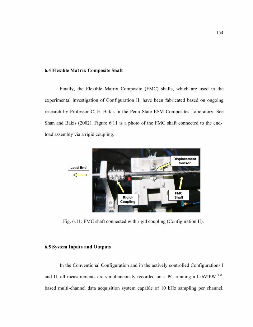
154

6.4 Flexible Matrix Composite Shaft

Finally, the Flexible Matrix Composite (FMC) shafts, which are used in the

experimental investigation of Configuration II, have been fabricated based on ongoing

research by Professor C. E. Bakis in the Penn State ESM Composites Laboratory. See

Shan and Bakis (2002). Figure 6.11 is a photo of the FMC shaft connected to the end-

load assembly via a rigid coupling.

6.5 System Inputs and Outputs

In the Conventional Configuration and in the actively controlled Configurations I

and II, all measurements are simultaneously recorded on a PC running a LabVIEW TM,

based multi-channel data acquisition system capable of 10 kHz sampling per channel.

FMCShaft

Load-End

Rigid-Coupling

DisplacementSensor

Fig. 6.11: FMC shaft connected with rigid coupling (Configuration II).

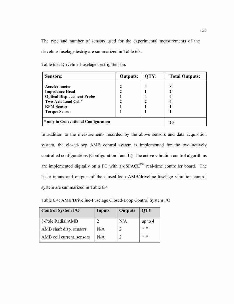
155

The type and number of sensors used for the experimental measurements of the

driveline-fuselage testrig are summarized in Table 6.3.

In addition to the measurements recorded by the above sensors and data acquisition

system, the closed-loop AMB control system is implemented for the two actively

controlled configurations (Configuration I and II). The active vibration control algorithms

are implemented digitally on a PC with a dSPACETM real-time controller board. The

basic inputs and outputs of the closed-loop AMB/driveline-fuselage vibration control

system are summarized in Table 6.4.

Table 6.3: Driveline-Fuselage Testrig Sensors

Sensors: Outputs: QTY: Total Outputs:

Accelerometer 2 4 8Impedance Head 2 1 2Optical Displacement Probe 1 4 4Two-Axis Load Cell* 2 2 4RPM Sensor 1 1 1Torque Sensor 1 1 1

20* only in Conventional Configuration

Table 6.4: AMB/Driveline-Fuselage Closed-Loop Control System I/O

Control System I/O Inputs Outputs QTY

8-Pole Radial AMB

AMB shaft disp. sensors

AMB coil current. sensors

2

N/A

N/A

N/A

2

2

up to 4

“ ”

“ “

156

Chapter 7

EXPERIMENTAL INVESTIGATION

7.1 Introduction

The first objective of the experimental investigation is to validate the

comprehensive tailrotor driveline-fuselage analytical model developed in Chapter 2. The

investigation will compare analytical predictions with experimental measurements of the

conventionally configured driveline-fuselage structure under various operating conditions

and shaft speeds. In particular, the experimental investigation will focus on validation of

the misalignment and torque-induced periodic parametric and forcing terms due to NCV

couplings. The second objective is to implement and evaluate the stability, performance,

and robustness of the closed-loop vibration control laws developed in this research for the

actively controlled Configurations I and II.

157

7.2 NCV-Drivel ine Model Validation

The driveline model evaluation and validation is performed on the driveline in the

Conventional Configuration and is conducted in two main phases. Figure 7.1 shows the

schematic of the experimental setup used for driveline model validation. Furthermore the

Testrig driveline setup details are summarized in Table 7.1.

In the first phase, the driveline-foundation structural model is validated without any

rotor-dynamic effects i.e. for Ω = 0 RPM. In the second phase, effects of misalignment

and load-torque on the Testrig driveline dynamics are experimentally investigated over a

range of shaft speeds and then compares with analytical predictions.

Data Acquisition

PC #132 Channel DAQ10 kHz Sampling

Rate/Channel

Multi-channelAA Filter +

Signal Conditioner

Fig. 7.1: Testrig setup for experimental validation of driveline analytical model.

Shaker

A B C

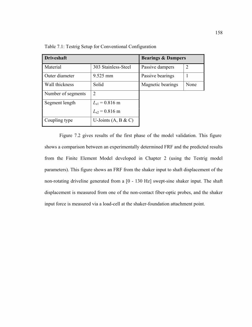
158

Figure 7.2 gives results of the first phase of the model validation. This figure

shows a comparison between an experimentally determined FRF and the predicted results

from the Finite Element Model developed in Chapter 2 (using the Testrig model

parameters). This figure shows an FRF from the shaker input to shaft displacement of the

non-rotating driveline generated from a [0 - 130 Hz] swept-sine shaker input. The shaft

displacement is measured from one of the non-contact fiber-optic probes, and the shaker

input force is measured via a load-cell at the shaker-foundation attachment point.

Table 7.1: Testrig Setup for Conventional Configuration

Driveshaft Bearings & Dampers

Material 303 Stainless-Steel Passive dampers 2

Outer diameter 9.525 mm Passive bearings 1

Wall thickness Solid Magnetic bearings None

Number of segments 2

Segment length Ls1 = 0.816 m

Ls2 = 0.816 m

Coupling type U-Joints (A, B & C)

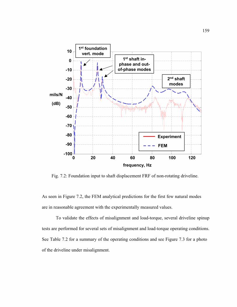
159

As seen in Figure 7.2, the FEM analytical predictions for the first few natural modes

are in reasonable agreement with the experimentally measured values.

To validate the effects of misalignment and load-torque, several driveline spinup

tests are performed for several sets of misalignment and load-torque operating conditions.

See Table 7.2 for a summary of the operating conditions and see Figure 7.3 for a photo

of the driveline under misalignment.

0 20 40 60 80 100 120-100

-90

-80

-70

-60

-50

-40

-30

-20

-10

0

10

mils/N

(dB)

frequency, Hz

FEM

Experiment

1st shaft in-phase and out-of-phase modes

1st foundationvert. mode

2nd shaftmodes

Fig. 7.2: Foundation input to shaft displacement FRF of non-rotating driveline.

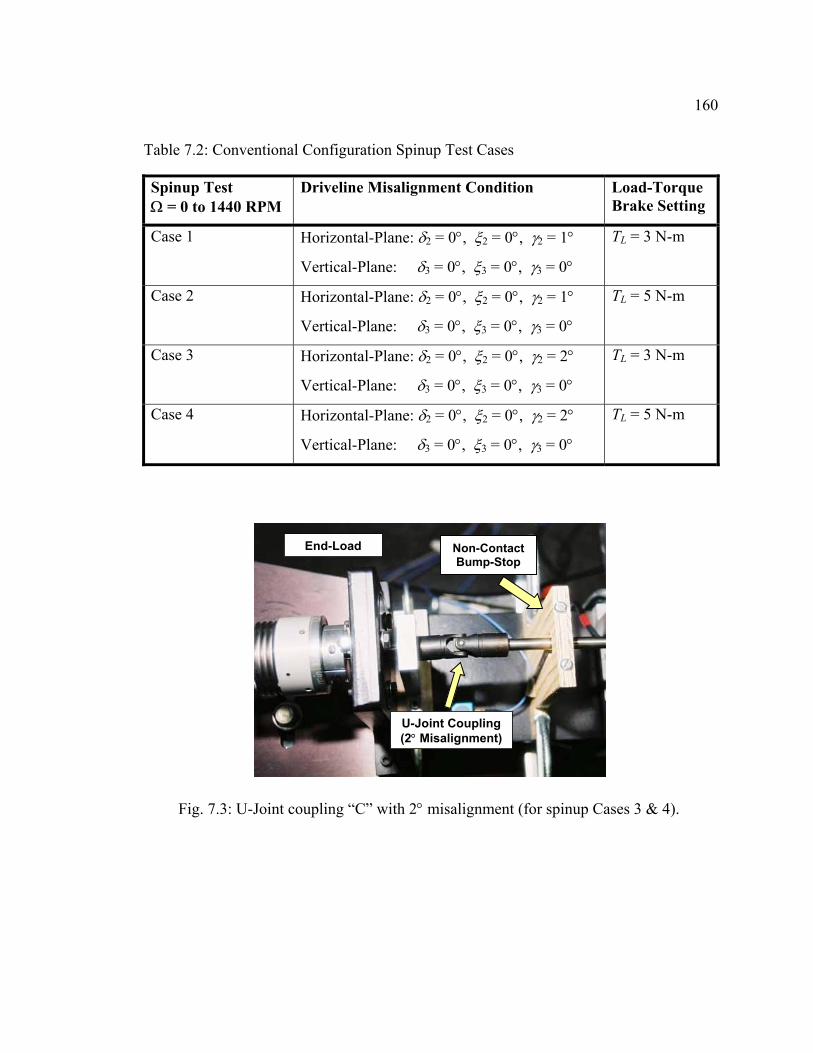
160

Table 7.2: Conventional Configuration Spinup Test Cases

Spinup TestΩ = 0 to 1440 RPM

Driveline Misalignment Condition Load-TorqueBrake Setting

Case 1 Horizontal-Plane: δ2 = 0°, ξ2 = 0°, γ2 = 1°

Vertical-Plane: δ3 = 0°, ξ3 = 0°, γ3 = 0°

TL = 3 N-m



TL = 5 N-m



TL = 3 N-m



TL = 5 N-m

End-Load

U-Joint Coupling(2° Misalignment)

Fig. 7.3: U-Joint coupling “C” with 2° misalignment (for spinup Cases 3 & 4).

Non-ContactBump-Stop

161

Figure 7.4 shows the load-torque and the shaft speed time histories for the

conventional configuration spinup test cases. Here, the load-torque has both static and

shaft speed dependent portions. The static portion of the load-torque is due to the brake

torque setting, and, it is hypothesized that, the speed dependent portion is due to gearbox

oil viscosity effects. In order to ensure a more accurate model validation, this measured

load-torque with the shaft speed dependence is incorporated into the time-domain spinup

simulations.

Figure 7.5 shows the shaft vibration response for two different spinup test cases as

measured by one of the fiber-optic displacement probes. Further, Figure 7.6 shows a

time-frequency spectrogram of the shaft response for spinup Case 4.

Time, sec

Time, sec

0 20 40 60 80 100 120 140 160 180 200 2200

2

4

6

Load

-Tor

que,

N-m Cases 1 & 3

Cases 2 & 4

0 20 40 60 80 100 120 140 160 180 200 2200

5

10

15

20

25

Shaf

t Spe

ed, H

z

Cases 1, 2, 3 & 4

Fig. 7.4: Load-torque and shaft speed vs. time (spinup experiment Cases 1 - 4).

162

As expected, due to the LPTV nature of the equations-of-motion derived in Chapter 2 and

from the harmonic balance analysis conducted in Chapter 4, the response spectrum is

concentrated at integer multiples of the shaft speed, NΩ. In particular, the shaft imbalance

contributes to the synchronous portion of the response at the shaft speed Ω, while the

misalignment and load-torque cause super-synchronous vibration at the 2Ω, 3Ω and 4Ω

harmonics. The remaining response bands at non-integer multiples of Ω are due to

gearbox meshing excitations originating from the end-load assembly.

0 20 40 60 80 100 120 140 160 180 200-50

0

50

Time, sec

0 20 40 60 80 100 120 140 160 180 200-50

0

50

Shaf

t Dis

plac

emen

t, m

ils

Case 4

Case 1

Time, Sec

Fig. 7.5: Shaft displacement vs. time (spinup experiment Cases 1 & 4).

163

To investigate the accuracy of the NCV-driveline analytical model with respect to

misalignment and load-torque effects, time-domain simulations for spinup Cases 1-4 are

performed using the model and compared with experimental results. The results of this

comparison are shown in Figures 7.7 and 7.8. Figure 7.7 shows the 2Ω displacement

response amplitudes for spinup Cases 1-4 for a point on the shaft, and Figure 7.7 shows

the 2Ω acceleration response amplitudes for a point on the foundation beam.

4Ω 2Ω

Ω

Fig. 7.6: Spectrogram of shaft response, spinup experiment Case 4.

3Ω

164

0 5 10 15 2025

12

340

10

20

30

40

05

1015

2025

12

340

10

20

30

40

Mils

Mils

Case #

Case #

Shaft Speed, Hz

Shaft Speed, Hz

Case #1) Mis. = 1°, TLmax = 3.0 N-m2) Mis. = 1°, TLmax = 5.0 N-m3) Mis. = 2°, TLmax = 3.0 N-m4) Mis. = 2°, TLmax = 5.0 N-m

2/rev Shaft Disp.(Experiment)

2/rev Shaft Disp.(FEM)

Fig. 7.7: Shaft displacement at frequency 2Ω for spinup Cases 1-4, FEM & Exp.

05

1015

2025

12

34

0

0.005

0.01

0.015Case #1) Mis. = 1°, TLmax = 3.0 N-m2) Mis. = 1°, TLmax = 5.0 N-m3) Mis. = 2°, TLmax = 3.0 N-m4) Mis. = 2°, TLmax = 5.0 N-m

Shaft Speed, Hz

05 10 15 20

25

12

34

0

0.005

0.01

0.015

Shaft Speed, Hz

Case #

Case #

g

g

2/rev FoundationAccel. (Experiment)

2/rev FoundationAccel. (FEM)

Fig. 7.8: Foundation acceleration at frequency 2Ω for spinup Cases 1-4, FEM & Exp.

165

These comparisons indicate that the comprehensive driveline analytical model

developed in Chapter 2 reasonably predicts effects of imbalance, misalignment and load-

torque on the driveline dynamics. This validation of the analytical model reinforces both

the novel misalignment induced stability/instability behavior discovered in Chapter 3 and

the Configurations I and II closed-loop results and conclusion presented in Chapters 4

and 5.

7.3 Active Controller Experimental Implementation

To experimentally implement the actively controlled driveline Configurations I

and II on the Testrig, a combination of digital active controller hardware is utilized. Both

the Configuration I and II hybrid control strategies are combinations of a real-time

feedback control loop and a slowly updating harmonic adaptive vibration control (AVC).

Since the feedback and the adaptive control loops have different sampling rate

requirements, they are implemented on separate hardware and then combined and

injected into the AMB-driveline system as the hybrid control law, u = uFB + uAVC. The

feedback portion of the Configuration I and II controllers are implemented on a

Revolve multi-channel MB350T digital PID controller, while the harmonic adaptive

control (MHAVC for Config. I and SAVC for Config. II) is implemented on a dSPACE

model 1103 digital controller in conjunction with MATLAB Simulink and Real-Time

Workshop. See Figure 7.9 for a block diagram of the overall closed-loop AMB-

driveline Testrig system. Since the feedback portion of the control is a digital PID

166

controller with low-pass filtering and lead-lag compensation, the feedback portions of

the Configurations I and II controllers are not identical to the ones developed in Chapters

4 and 5. Despite these hardware limitations, as long as the digital feedback controlled

AMB-Driveline subsystem is BIBO stable, the performance and convergence robustness

of harmonic adaptive vibration control strategies (SAVC and MHAVC) can be evaluated

and assessed experimentally.

Figure 7.10 shows the basic elements of the open-loop Testrig AMB/driveline system.

AMB/Driveline System

Digital PID FeedbackController

Adaptive Vibration Controller(SAVC or MHAVC)

uAVC

Ts

+

uFB

Ts

u

d z

y

y

Ω

ibias

Fig. 7.9: Experimentally implemented hybrid feedback/harmonic adaptive controller.

167

7.3.1 PID Feedbac k Control Implementation

Figure 7.11 gives the overall structure of the digital PID feedback controller

utilized in the experimental implementation.

To determine the PID feedback control parameters for the Configurations I and II Testrig

drivelines that achieve robustly stable levitation, the stability for a range of controller

parameters is calculated using the driveline analytical model. Using the stability analysis

Power Amplifier famb

“negative stiffness” feedbackloop due to magnetic levitationAMB/Driveline System

AMB

y

y

d

ibias

u

DrivelineSystem

z

icoil

Fig. 7.10: Open-Loop Testrig AMB/driveline system.

Lead-Lag Filter

Low-Pass Filter

PD Filter

Integrator

+

uFB

Digital PID Feedback Controller

y

Fig. 7.11: Digital PID controller for Configuration I and II feedback control loop.

168

results as a guide, various sets of PID controller parameters from the predicted sub-set

of stabilizing control parameters are tested experimentally. The results of this

analysis/trial-and-error process are summarized in Table 7.3, which shows the sets of

digital PID controller parameters that experimentally achieve stable closed-loop

levitation of the Configuration I and II Testrig drivelines. These values are utilized in the

subsequent experimental investigation of Configuration I and II.

In Configuration I, it is found that three AMBs (namb = 3) are sufficient to achieve stable

levitation, while in Configuration II, four AMBs (namb = 4) are required due to the

increased lateral flexibility of the FMC shafting.

Both the Testrig stability analysis and experimental results show that the

levitation stability of Configuration II (AMB-FMC driveline) is much more sensitive to

the PID controller parameters compared with Configuration I (AMB-NCV alloy

Table 7.3: Configuration I and II Digital PID Controller Parameters

Digital PID Controller Parameters Configuration I Configuration II

Sampling Period, Ts

Bias current, ibias

Active Stiffness Gain, kp

Active Damping Gain kd

Integrator Gain, ki

Lead-lag filter pole, pLL

Lead-lag filter zero, zLL

Low-pass filter cutoff, ωLP

Low-pass filter damping ratio, ζLP

1/10000 sec

1.0 Amps

5000 Amps/m

4.0 Amps-sec/m

1000 Amps/m-sec

200 Hz

100 Hz

800 Hz

0.707

1/10000 sec

0.55 Amps

4000 Amps/m

2.5 Amps-sec/m

1000 Amps/m-sec

280 Hz

170 Hz

800 Hz

0.707

169

driveline). Consequently, for the same bias current level, ibias, the region of

stabilizing PID control gains is much larger for Testrig Configuration I compared with

Testrig Configuration II. For Configuration I, an acceptable PID controller design was

achieved with ibias=1.0 Amp. However, an acceptable PID controller design for

Configuration II could only be achieved for a reduced bias current level, ibias=0.55 Amp.

According to (2.69) – (2.72), the maximum AMB actuation force, Fmax, is

2

2

max 4gap

biasb

h

iGF = ( 7.1 )

and the negative stiffness due to magnetic levitation is

3

24

gap

biasbx

h

iGk = ( 7.2 )

Thus, the reduced bias current level in Configuration II translates into less negative

stiffness but also means less available actuation authority.

Through analytical investigation, it is concluded that the difficulties encountered

in achieving stable levitation of the AMB-FMC Testrig driveline at higher bias current

levels (ibias > 0.6 Amp) is a result of the relatively large AMB rotor-to-shaft mass ratio, µr

= Mrotor /Mshaft, of the Configuration II Testrig driveline. See Table 7.4.

170

The relatively large AMB rotor mass ratio, µr = 0.89, of Testrig Configuration II

represents an extreme case and is not true in general of AMB-FMC drivelines. In

particular, as the driveline scale increases, µr tends to decrease (e.g. µr = 0.054 for the full

scale AH-64 Configuration II driveline). Thus, the Configuration II Testrig driveline

levitation difficulties encountered at higher bias current levels are an artifact of the

particular testrig scaling and not a general problem inherent to AMB-FMC driveline

systems.

Prior to driveline operation, the closed-loop transfer functions of the non-rotating

(Ω = 0 RPM) magnetically levitated Configrtaion I and II driveline systems are

characterized. Specifically, by injecting white noise disturbances into the AMB control

inputs, the control-path transfer functions, Gnm(jω), from the AMB control inputs, u, to

the measured shaft displacements, y, are characterized.

)()(

)(ωω

ωjUjY

jGm

nnm = ( 7.3 )

Table 7.4: AH-64 and Testrig Driveline Mass Properties

AH-64 Driveline Testrig Driveline

Config. I Config. II Config. I Config. II

Mass of shafting, Mshaft 10.91 kg 11.88 kg 1.222 kg 0.316 kg

Mass of AMB rotor, Mrotor 0.645 kg 0.645 kg 0.28 kg 0.28 kg

AMB rotor mass ratio, µr 0.06 0.054 0.23 0.89

171

Where indices n and m range from [1, …, 2namb]. Figure 7.12 shows a comparison

between the analytically and experimentally determined control-path transfer functions

for the Configuration I Testrig driveline.

7.3.2 Harmonic Adaptive Control Implementation

The adaptive portions of the control in Configuration I and II are implemented on

a dSPACE digital controller board which has 20 analog input channels and 8 analog

output channels. Specifically, Figure 7.13 is a block diagram of the harmonic adaptive

vibration control (AVC), which is composed of three main sub-blocks.

Experiment

FEM

0 20 40 60 80 100 120 140 160 180 2000

250

500

750

10000 20 40 60 80 100 120 140 160 180 2000

500

1000

1500

20000 20 40 60 80 100 120 140 160 180 2000

500

1000

1500

2000

Frequency, Hz

|G11( jω )|(µ m/Amps)



Operating Conditions:Ω = 0 RPMTL = 0 Nmθ = 0 °

Control Law:PID Feedback

AMB1

AMB2

AMB3

Fig. 7.12: Testrig Configura tion I closed-loop control-path transfer functions.

172

The first sub-block, shown in Figure 7.14, is the Harmonic Fourier Coefficient (HFC)

calculator.

This block computes the steady-state response HFC vector, Yi, after each AVC update.

Here, Yi, is

TThnc

Thns

Tc

TsiY ][ 11 yyyy K= ( 7.4 )

which corresponds to the steady-state shaft vibration response, y(t).

[ ]∑=

Ω+Ω+=hn

nncns tntnty

100 )cos()sin()( yyy0 ( 7.5 )

Due to the presence of measurement noise, e(t), the measured shaft response is

AVCSynthesis

iY

1+iU]ˆˆ[ˆ]ˆˆ[ 1

1 iiyuT

yuyuT

yui YUTTTTU += −+

HFCCalculator

)(tuAVC

Ω Ω

)(ty+

)(te

Fig. 7.13: Harmonic adaptive vibration control.

iY2

Multi-ChannelMoving AverageLow-Pass Filter

M

)sin( skTΩ

)cos( skTΩ

)sin( sh kTn Ω

)cos( sh kTn Ω

MU

X

Tconv

Tupdate Ts

)(ty+

)(te

Fig. 7.14: Harmonic Fourier Coefficient calculator block.

173

)()()(ˆ tetyty += ( 7.6 )

Based on the measurements )(ˆ ty , the estimate of the response HFC vector,

TThnc

Thns

Tc

TsiY ]ˆˆˆˆ[ˆ

11 yyyy K= ( 7.7 )

is computed in real-time at each desired shaft speed harmonic, mΩ, via a moving average

convolution scheme given by

],...,1[

)cos()(ˆ 2ˆ

)sin()(ˆ 2ˆ

conv

0conv

conv

0conv

hT

mc

T

ms

nm

dttmtyT

dttmtyT

=

Ω=

Ω=

∫

∫

y

y

( 7.8 )

Where Tconv is the convolution window history length, see Figure 7.16. By selecting Tconv

= Np Tp, where Tp = 2π/Ω is the shaft rotation period and Np is some integer number of

revolutions, the resulting estimated sin and cosine Fourier coefficient vectors, msy and

mcy , of the mth response harmonic are

],...,1[

)cos()(2 1ˆ

)sin()(2 1ˆ

0

0h

pTpN

ppmcmc

pTpN

ppmsms

nm

dttmteTN

dttmteTN

=

Ω+=

Ω+=

∫

∫

yy

yy

( 7.9 )

Assuming the measurement noise, e(t), is stationary with

2)](var[ ,0)]([ eteteE σ== (7.10)

where E[ ] is the expectation operator and var[ ] is the variance, the resulting estimated

Fourier coefficient vectors have a Gaussian distribution with the following statistics.

174

] ..., 1, [

2

][ var,]ˆ[

2

][ var,]ˆ[

2

2

h

pp

emcmcmc

pp

emsmsms

nm

TNyyyE

TNyyyE

=

==

==

σ

σ

(7.11)

Using the estimated response HFC vector, iY , together with the AVC update law

(defined in Chapter 4), the second sub-block updates the AVC control input HFC vector,

Ui+1. Finally, the AVC control input, Ui+1, is transformed into the time-domain via the

convolutions in the Harmonic AVC Synthesis block. See Figure 7.15,

Refer to Appendix G for complete Simulink block diagrams of the controller.

Figure 7.16 is a schematic representation of the time-domain response of a

system with slowly updating harmonic AVC inputs. Here Ts is the real-time sampling

period, which is selected to satisfy the Nyquist sampling criteria i.e. 1/ Ts >> 2 fbw where

fbw is the shaft response bandwidth in Hz. Furthermore, the AVC update period, Tupdate, is

chosen such that Tupdate = Tdecay +Tconv where Tdecay is the transient setting-time of the PID

controlled AMB-driveline sub-system. This ensures that system reaches a new steady-

1+iUM

+

+

+

M

DEM

UX

)sin( skTΩ

)cos( skTΩ

)sin( sh kTn Ω

)cos( sh kTn Ω

ZOH)(tuAVC

Fig. 7.15: Harmonic AVC synthesis block.

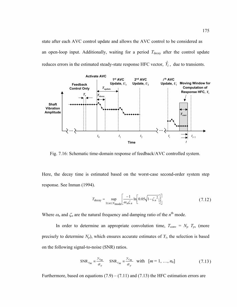
175

state after each AVC control update and allows the AVC control to be considered as

an open-loop input. Additionally, waiting for a period Tdecay after the control update

reduces errors in the estimated steady-state response HFC vector, iY , due to transients.

Here, the decay time is estimated based on the worst-case second-order system step

response. See Inman (1994).

−

−=

≤≤

2

mode1decay 105.0ln1sup n

nnNnT ζ

ζω (7.12)

Where ωn and ζn are the natural frequency and damping ratio of the nth mode.

In order to determine an appropriate convolution time, Tconv = Np Tp, (more

precisely to determine Np), which ensures accurate estimates of Yi, the selection is based

on the following signal-to-noise (SNR) ratios.

e

mcmc

e

msms

yy

σσ≡≡ SNR SNR with [m = 1, …, nh] (7.13)

Furthermore, based on equations (7.9) – (7.11) and (7.13) the HFC estimation errors are

ShaftVibration

Amplitude

t0

Tupdate

… …

Activate AVC

Time

Ts Tdecay

1st AVCUpdate, U1

Tconv

t1 t2

tti+1

Moving Window forComputation of

Response HFC, Yi

ti

2nd AVCUpdate, U2

i th AVCUpdate, UiFeedback

Control Only

Fig. 7.16: Schematic time-domain response of feedback/AVC controlled system.

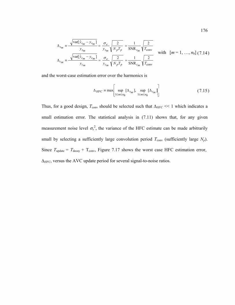
176

conv

conv

2SNR

1 2 ]ˆ[var

2SNR

1 2 ]ˆ[var

TTNyy

yy

TTNyy

yy

mcppmc

e

mc

mcmcmc

msppms

e

ms

msmsms

==−

≡∆

==−

≡∆

σ

σ

with [m = 1, …, nh] (7.14)

and the worst-case estimation error over the harmonics is

∆∆≡∆

≤≤≤≤][sup ],[supmax

11mc

hnmms

hnmHFC (7.15)

Thus, for a good design, Tconv should be selected such that ∆HFC << 1 which indicates a

small estimation error. The statistical analysis in (7.11) shows that, for any given

measurement noise level σe2, the variance of the HFC estimate can be made arbitrarily

small by selecting a sufficiently large convolution period Tconv (sufficiently large Np).

Since Tupdate = Tdecay + Tconv, Figure 7.17 shows the worst case HFC estimation error,

∆HFC, versus the AVC update period for several signal-to-noise ratios.

177

In Configuration I, the adaptive control attempts to suppress both the synchronous

imbalance response and the super-synchronous harmonic NCV effects (MHAVC). In

Configuration II, since the NCV effects are eliminated by the use of rigid couplings, only

the synchronous response will be suppressed (SAVC). Table 7.5 summarizes the

parameters utilized in the experimental implementation of the AVC control in each

configuration.

0 1 2 3 4 50

0.1

0.2

0.3

0.4

0.5

Tdecay Tupdate , sec

SNR=100

SNR=25

SNR=10

SNR=5

Signal-to-Noise Ratio:SNR = SNRsm or SNRcm

HFC∆

Fig. 7.17: HFC estimation error vs. AVC update time for several signal-to-noise ratios.

178

Furthermore, the update law dependents on the HFC mapping from Ui, to Yi. The actual

HFC mapping, yuT , depends on the driveline operating conditions. However, as shown

with the robust convergence and performance analyses in Chapters 4 and 5, the AVC

update law can be successfully approximated by using the HFC map of the levitated non-

rotating system yuT . To implement Configurations I and II, yuT is estimated offline with

batch least-squares system identification of the non-rotating, levitated, PID feedback

controlled driveline. Specifically, a set of p >> 2nunh randomly generated HFC input

vectors, Ui, is injected into the system and the corresponding response HFC vector, Yi. is

stored. Finally, the estimate, yuT , is obtained via (7.16).

11111 ]][[]][[ˆ

−

= T

ppT

ppyu UUUUUUYYT LLLL ( 7.16 )

To gauge the vibration performance and the control effort, the following root mean

square (RMS) metrics, yrms and irms, are defined for the entire system.

∑ ∫=

=yn

i

pTpNi

ppyrms dty

TNny

1 0

211 and ∑ ∫=

=un

i

pTpNi

ppurms dtu

TNni

1 0

211 ( 7.17 )

Table 7.5: Configuration I and II AVC Parameters

Harmonic Adaptive Vibration

Controller Parameters

Configuration I

(MHAVC)

Configuration II

(SAVC)

Number of Harmonics, nh 4 1

Harmonics to be suppressed Ω, 2Ω, 3Ω, 4Ω Ω

Update Period, Tupdate 3 sec 3 sec

Convolution Period, Tconv 1 sec 1 sec

179

7.4 Experimental Results: Configuration I with PID-MHAVC Control

Figure 7.18 and Table 7.6 show the experimental setup used for the

Configuration I experimental investigation.

Table 7.7 shows the different test cases which were conducted in Configuration I.

AMB1

U-Joint B

AMB2 AMB3

U-Joint A U-Joint C

Lamb1

Lamb2

Lamb3

Steel Shaft

Fig. 7.18: Testrig setup for Configuration I experiment.

Table 7.6: Configuration I Testrig Setup


Material 303 Stainless-Steel Passive dampers none

Outer diameter 9.525 mm Passive bearings none

Wall thickness Solid Magnetic bearings 3 AMB

Number of segments 2

Segment length Ls1 = 0.816 m

Ls2 = 0.816 m

AMB location Lamb1 = 0.2 Ls1

Lamb2 = Ls1 + 0.1 Ls2

Lamb3 = Ls1 + 0.8 Ls2

Couplings 3 U-Joints

180

The resulting RMS vibration and control current metrics for the Configuration I test cases

under PID and PID-MHAVC control are summarized in Figures 7.19 and 7.20 .

Table 7.7: Configuration I Experiment Test Cases

Case Number Shaft Speed Load-Torque Misalignment (All Cases)

Case 1 Ω = 10.3 Hz TL = 1.76 N-m

Case 2 Ω = 16.3 Hz TL = 2.09 N-m

Case 3 Ω = 22.2 Hz TL = 2.64 N-m

Low

Torque

Cases

Case 4 Ω = 30.1 Hz TL = 3.04 N-m

Horizontal-Plane:

δ2 = 0°, ξ2 = 0°, γ2 = 3°

Vertical-Plane:

δ3 = 0°, ξ3 = 0°, γ3 = 0°

Case 5 Ω = 10.0 Hz TL = 5.03 N-m

Case 6 Ω = 16.0.Hz TL = 5.16 N-m

Case 7 Ω = 22.5 Hz TL = 5.21 N-m

High

Torque

Cases

Case 8 Ω = 30.3 Hz TL = 5.27 N-m

RM

S V

ibra

tion,

µm

1 2 3 4 5 6 7 80

10

20

30

40

50

60

70PIDPID-MHAVC

Case Number

Fig. 7.19: RMS vibration metric for Configuration I experiment.

181

The time-domain response for each of the experiment test cases is given in Appendix G.

In particular, Figures 7.21 and 7.22 give the vibration and control current responses for

Case 6, where the results are similar to the remain test cases.

RM

S C

ontr

ol C

urre

nt, A

mp

1 2 3 4 5 6 7 80

0.05

0.1

0.15

0.2

0.25

0.3

PIDPID-MHAVC

Case Number

Fig. 7.20: RMS control current metric for Configuration I experiment.

182

0 50 100 150 200-225

0

225

0 50 100 150 200-225

0

225

0 50 100 150 200-225

0

225

0 50 100 150 200-225

0

225

0 50 100 150 200-225

0

225

0 50 100 150 200-225

0

225

v-di

r di

sp.

AM

B3,

µm

PID PID-MHAVC

v-di

r di

sp.

AM

B2,

µm

v-di

r di

sp.

AM

B1,

µm

Activate MHAVC w-d

ir d

isp.

AM

B3,

µm

w-d

ir d

isp.

AM

B2,

µm

w-d

ir d

isp.

AM

B1,

µm

time, sec

Fig. 7.21: Shaft response, Configuration I experiment Case 6.

0 50 100 150 200

-0.2

0

0.2

0.4

0 50 100 150 200

0

0.2

0.4

0.6

0 50 100 150 200

-0.1

0

0.1

0 50 100 150 200

-0.1

0

0.1

0.2

0 50 100 150 200

-0.8

-0.6

-0.4

-0.2

0 50 100 150 200-0.4-0.2

00.20.4

Activate MHAVC

time, sec

v-di

r cu

rren

t.A

MB

3, A

mps

v-di

r cu

rren

t.A

MB

2, A

mps

v-di

r cu

rren

t.A

MB

1, A

mps

w-d

ir c

urre

nt.

AM

B3,

Am

psw

-dir

cur

rent

.A

MB

2, A

mps

w-d

ir c

urre

nt.

AM

B1,

Am

ps

Fig. 7.22: Control currents, Configuration I experiment Case 6.

183

Finally, Figure 7.23 shows the spectrum of a typical Configuration II response.

The experimental results for Configuration I demonstrate that PID-MHAVC control

strategy achieves significant vibration suppression of imbalance, misalignment and load-

torque induced vibrations. Since vibration suppression was achieved for all test cases

without knowledge of misalignment, load-torque or imbalance utilized in the control law,

the robustness claims made in Chapter 4 are experimentally confirmed. Additionally, by

examining the control currents in Figures 7.20 and 7.22, the experiment results show

that the PID-MHAVC control requires less control current than the PID baseline control.

0 20 40 60 80 100 120 1400

1020304050

0 20 40 60 80 100 120 1400

1020304050

0 20 40 60 80 100 120 1400

1020304050

0 20 40 60 80 100 120 1400

1020304050

0 20 40 60 80 100 120 1400

1020304050

0 20 40 60 80 100 120 1400

1020304050

Frequency, Hz

Shaf

t Vib

ratio

n A

mpl

itude

, µm

(PI

D)

w-dir response at AMB1PID Control



w-dir response at AMB1PID-MHAVC Control



Shaf

t Vib

ratio

n A

mpl

itude

, µm

(PI

D-M

HA

VC

)

Ω2Ω

3Ω4Ω

128.2 µm“peak”

79.3 µm“peak”

Fig. 7.23: Shaft response spectra, Configuration I experiment Case 6.

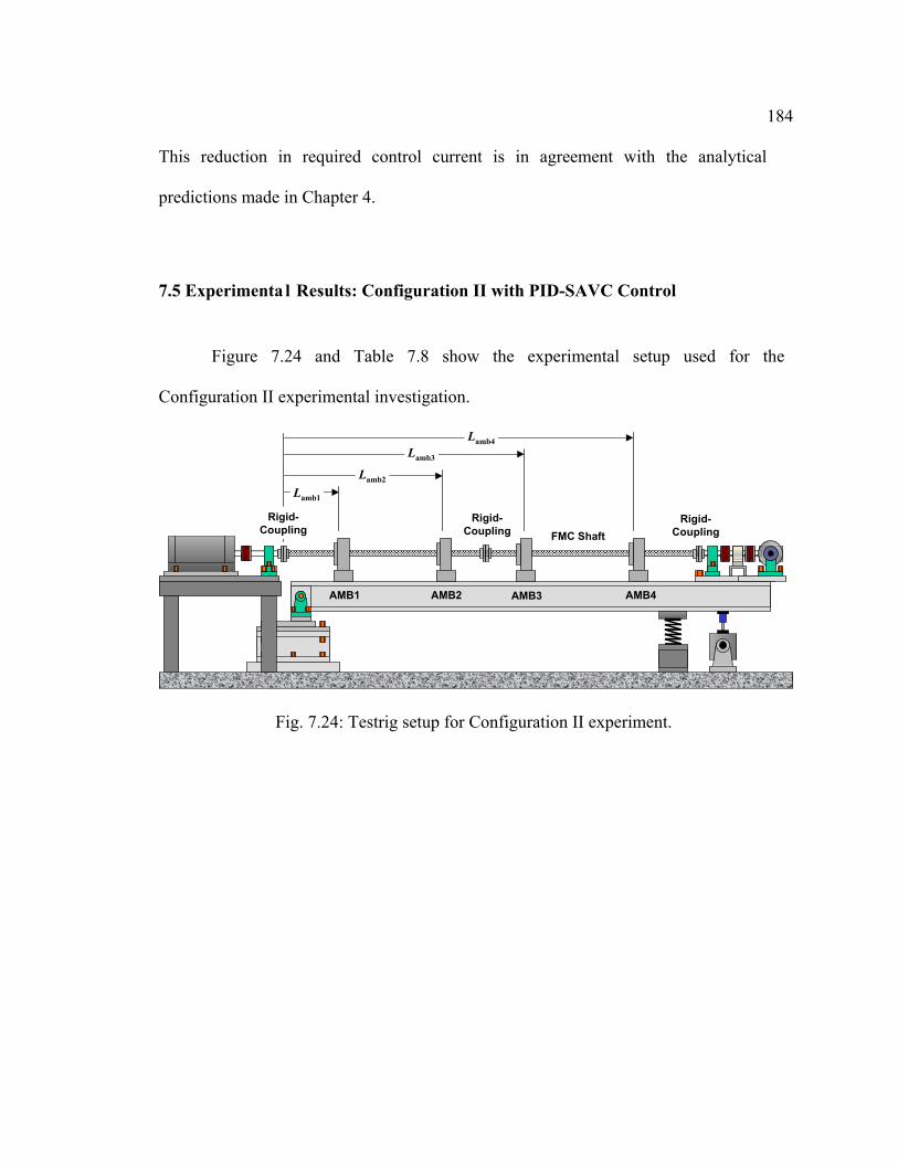
184

This reduction in required control current is in agreement with the analytical

predictions made in Chapter 4.

7.5 Experimenta l Results: Configuration II with PID-SAVC Control

Figure 7.24 and Table 7.8 show the experimental setup used for the

Configuration II experimental investigation.

Rigid-Coupling

Rigid-Coupling

AMB1 AMB2 AMB4

Rigid-Coupling

Lamb1

Lamb2

Lamb3

AMB3

FMC Shaft

Lamb4

Fig. 7.24: Testrig setup for Configuration II experiment.

185

Table 7.9 gives the different test cases which were conducted in the Configuration II

experimental investigation.

Here, the Configuration II experiment is conducted at three different operating speeds i.e.

Cases 1–3. However, due to several limitations of the testrig hardware in Configuration

II, no driveline misalignment (δ2 =ξ2 = γ2 = δ3 =ξ3 = γ3 = 0°) and no load-torque (TL = 0

Table 7.8: Configuration II Testrig Setup


Passive dampers nonematerial FMCa with Ply layer

angles [45°/-45°/-90°/90°] Passive bearings none

outer diameter 9.525 mm Magnetic bearings 4 AMB

wall thickness 0.75 mm

Number of

segments

2

AMB Location Lamb1 = 0.2 Ls1

Lamb2 = Ls1 + 0.1 Ls2

Lamb3 = Ls1 + 0.8 Ls2

Lamb3 = Ls1 + 0.8 Ls2Segment length Ls1 = 0.819 m

Ls2 = 0.851 m

Couplings 3 Rigid (Clamp-Type)

Table 7.9: Configuration II Experiment Test Cases


Case 1 Ω = 10.0 Hz TL = 0 N-m

Case 2 Ω = 15.0 Hz TL = 0 N-m

Case 3 Ω = 25.0 Hz TL = 0 N-m

Horizontal-Plane:

δ2 = 0°, ξ2 = 0°, γ2 = 0°

Vertical-Plane:

δ3 = 0°, ξ3 = 0°, γ3 = 0°

186

N-m) is applied during the tests. Unlike Configuration I with flexible-couplings to

accommodate the misalignments, in Configuration II misalignments produce shaft

curvature. Due to the relatively large AMB length - shaft length ratio that occurs at the

testrig scale, shaft curvature within the AMB causes internal AMB rotor/stator clearance

problems. of this issue. Therefore, only the aligned FMC driveline is explored in the

Configuration II experiment test cases. Furthermore, due to the low stiffness of the FMC

shaft material, the clamp-type rigid couplings used in the Configuration II Testrig

driveling did not achieve sufficient clamping force to allow transmission of the load-

torque without slippage. Therefore, the Configuration II experiment was conduced

without any applied load torque. Refer to Chapter 8 for more discussion and possible

future research related to these issues.

As shown from the analysis in Chapter 5, since there are no NCV effects in the

rigidly coupled FMC driveline system, the misalignment and load-torque do not

explicitly affect the Configuration II driveline dynamics (unlike Configuration I).

Therefore, the Configuration II experiment test Cases 1-3 are adequate to validate and

explore the converge behavior and the imbalance vibration suppression performance of

the feedback/SAVC controlled AMB-FMC driveline system. Specifically, the resulting

RMS vibration and control current metrics for the Configuration II test cases under PID

and PID-SAVC control are summarized in Figures 7.25 and 7.26.

187

1 2 30

10

20

30

40

50

60

70

80

90

100

Case Number

RM

S V

ibra

tion,

µm

PIDPID-SAVC

Backup-BearingContact

*

Fig. 7.25: RMS vibration metric for Configuration II experiment.

1 2 30

0.05

0.1

0.15

0.2

0.25

Case Number

RM

S C

ontr

ol C

urre

nt, A

mp

PIDPID-SAVC

Fig. 7.26: RMS control current metric for Configuration II experiment.

188

See Appendix G for the time-domain response data from each test case. In particular,

Figure 7.27 and Figure 7.28 give the vibration response and the corresponding response

spectrum for a particular case.

0 50 100 150 200 250 0 50 100 150 200 250

0 50 100 150 200 250 0 50 100 150 200 250

0 50 100 150 200 250 0 50 100 150 200 250

0 50 100 150 200 250 0 50 100 150 200 250

-225

0

225

-225

0

225

-225

0

225

-225

0

225

-225

0

225

-225

0

225

-225

0

225

-225

0

225

w-d

ir d

isp.

AM

B1,

µm

w-d

ir d

isp.

AM

B2,

µm

w-d

ir d

isp.

AM

B3,

µm

w-d

ir d

isp.

AM

B4,

µm

v-di

r di

sp.

AM

B1,

µm

v-di

r di

sp.

AM

B2,

µm

v-di

r di

sp.

AM

B3,

µm

v-di

r di

sp.

AM

B4,

µm PID PID-SAVC

Activate SAVC

time, sec

Fig. 7.27: Shaft response, Configuration II experiment Case 1.

189

The Configuration II experimental results shows that the response is concentrated at the

operating speed Ω. This is as expected since the are no NVC effects due to the use of

rigid couplings. Thus, only synchronous imbalance excitation is present in the system.

The experimental results for Configuration II also demonstrate that PID-SAVC control

achieves significant vibration suppression of imbalance vibration. Since this vibration

suppression is achieved for all test cases without knowledge of the imbalance, the PID-

SAVC successfully adapts and has robust performance characteristics. Also, similar to

Configuration I, and as predicted by the analysis in Chapter 5, the Configuration II

0 20 40 60 80 100 120 140

0 20 40 60 80 100 120 140

0 20 40 60 80 100 120 140

0 20 40 60 80 100 120 140

020406080

020406080

020406080

020406080

0 20 40 60 80 100 120 140

0 20 40 60 80 100 120 140

0 20 40 60 80 100 120 140

0 20 40 60 80 100 120 140

020406080

020406080

020406080

020406080

Frequency, Hz

Shaf

t Vib

ratio

n A

mpl

itude

, µm

(PI

D)

Shaf

t Vib

ratio

n A

mpl

itude

, µm

(PI

D-M

HA

VC

)





w-dir response at AMB1PID-SAVC Control




Ω

Fig. 7.28: Shaft response spectra, Configuration II experiment Case 1.

190

experimental results show that the feedback/SAVC control achieves vibration

suppression with less control current than the baseline feedback controlled system.

7.6 Experimental Investigation Summary and Conclusions

Utilizing the frequency-scaled driveline Testrig developed in this research, the

stability and performance of the conventionally configured driveline and the actively

controlled driveline configurations I and II are experimentally investigated over a range

of driveline operating conditions.

In the first phase of the investigation, the experimentally measured driveline

vibration is compared with analytical predictions under various misalignment, load-

torque and shaft speed operating conditions. The results of this comparison show that the

comprehensive driveline analytical model developed in Chapter 2 accurately predicts the

multi-harmonic driveline vibration response due NCV coupling kinematics, driveline

misalignment, and load-torque.

In the second phase of the investigation, the two actively controlled driveline

configurations I and II are experimentally implemented and evaluated using the driveline

Testrig and the AMB hardware. In Configuration I, the experimental results demonstrate

that the hybrid PID-MHAVC strategy developed in this thesis successfully adapts and

converges to suppress the multi-harmonic driveline vibration induced by misalignment,

load-torque and imbalance. Since no knowledge of the misalignment, load-torque or

imbalance is utilized in the control implementation, the experiment demonstrates the

robustness of the PID-MHAVC control strategy. Furthermore, the Configuration II

191

experiment demonstrates the successful operation of the AMB-FMC driveline system

and validates the robustness and the imbalance vibration suppression capabilities of the

PID-SAVC control strategy. Additionally, the experimental results from Configurations I

and II confirm the control current trends predicted by the analyses in Chapters 4 and 5.

Specifically, the experiments show that the PID-MHAVC and PID-SAVC strategies (in

Configurations I and II respectively) achieved vibration suppression without increasing

the overall RMS control current relative to the PID feedback controlled baseline.

Finally, the experimental results (see Appendix G) and the time-domain analysis

in Chapter 4 demonstrate that PID-MHAVC (and PID-SAVC) achieves approximately

95% convergence after two AVC update steps. Thus Tconvergence ≅ 2Tupdate. In the case of

the experiment, since Tupdate = 3 sec, the convergence time is Tconvergence = 6 sec. The AVC

convergence time is an important aspect of the control performance especially in a quasi-

steady environment where the driveline misalignment and load-torque operating

conditions are changing frequently. Figure 7.29 is a schematic plot of driveline load-

torque in a quasi-steady operating environment.

192

In the case of rotorcraft drivelines, such a quasi-steady operating environment occurs

during maneuvering flight. In particular, Horn, et al. (2002), showed that driveline load-

torque varied in a quasi-steady manner during various pull-up and pitch-over maneuvers.

In order for the adaptive driveline vibration control (MHAVC and SAVC) to be

beneficial during such maneuvers, the convergence time should less than the quasi-steady

operation periods. Horn, et al. (2002) showed that the quasi-steady operation periods can

be on the order of 10 to 15 seconds during aggressive pull-up and pitch-over maneuvers

and larger for less aggressive maneuvering. Therefore, PID-MHAVC and PID-SAVC

control with Tupdate = 3 sec (Tconvergence = 6 sec) would be adequate to suppress the

rotorcraft driveline vibration during maneuvering flight. Finally, based on the relation

between the SNR and Tupdate in (7.14) and in Figure 7.17, the AVC update and

convergence times could be further reduced by ensuring a sufficient SNR is present in the

control system.

100

50

0

Loa

d-T

orqu

e (%

)

time, sec

Quasi-SteadyOperation

Quasi-SteadyOperation

TransientOperation

Fig. 7.29: Driveline load-torque in quasi-steady operating environment.

193

Chapter 8

CONCLUSIONS AND RECOMMENDATIONS FOR FUTURE WORK

8.1 Summary and Conclusions

To advance the state-of-the-art of rotorcraft and other high-performance

drivelines, this thesis explores two novel actively controlled tailrotor driveline

configurations utilizing both AMB and FMC technologies. In the first configuration,

Configuration I, the conventional contact hanger-bearings and viscous shaft dampers are

replaced with non-contact AMB devices. In Configuration II, the conventional hanger-

bearings and viscous dampers are replaced with AMBs, and the conventional segmented

shaft and flexible-couplings are replaced with a rigidly coupled single-piece FMC shaft.

This research theoretically develops and experimentally validates novel hybrid robust-

adaptive vibration control strategies for both of the new actively controlled driveline

configurations based on their specific characteristics and uncertainties.

To facilitate analysis and development of the active control laws, a

comprehensive analytical model of the driveline system was developed for both driveline

194

configurations. The Configuration I model consists of a multi-segment flexible

driveshaft supported by magnetic bearings, and includes effects of rotating-frame

damping, magnetic field negative stiffness, imbalance, non-constant velocity flexible-

coupling kinematics, misalignment, load-torque and foundation flexibility. The

Configuration II model is similar but with the non-constant velocity flexible-coupling

kinematics removed and the FMC shaft modeled with classical lamination theory.

To experimentally validate the comprehensive tailrotor driveline-fuselage

analytical model and evaluate the closed-loop performance of the control algorithms

developed for Configurations I and II, a comprehensive, frequency-scaled, active

magnetic bearing controlled, multi-segment driveline-foundation testrig is designed and

constructed. The testrig driveline features adjustable misalignments, load-torque and

load-inertia, and is mounted on a flexible foundation beam structure coupled with

electromagnetic shaker. The testrig is fully instrumented with accelerometers, optical

encoder, eddy current probes, torque sensor, and three digitally controlled magnetic

bearings. Comparisons between analytical predictions and experimental results indicate

that the comprehensive driveline analytical model developed in this research successfully

predicts effects of imbalance, misalignment and load-torque on driveline dynamics.

The control strategy developed for Configuration I is based on a hybrid design

consisting of a PID feedback controller augmented with a slowly adapting, Multi-

Harmonic Adaptive Vibration Control (MHAVC). The MHAVC is based on a novel,

multi-harmonic Fourier coefficient transfer matrix representation of the linear periodic

time-varying driveline system obtained via a harmonic balance approach. From this, the

195

convergence condition and the relations for the converged response of the adaptive

control law was formulated.

Both the analytical and experimental results for Configuration I demonstrate that

the PID-MHAVC control strategy achieves significant multi-harmonic vibration

suppression of the synchronous imbalance, and the super-synchronous misalignment and

load-torque induced vibrations. Furthermore, since this vibration suppression was

achieved without knowledge of misalignment, load-torque or shaft imbalance condition,

the control strategy developed for the segmented AMB supercritical driveline system is

robust. Finally, both analysis and experiment demonstrate that, except near the closed-

loop natural frequencies, the PID-MHAVC achieved vibration suppression without

increasing the overall control current relative to the PID controlled baseline.

The control strategy developed for the AMB-FMC tailrotor driveline system

(Configuration II) is based on a hybrid H∞ feedback/Synchronous Adaptive Vibration

Control (SAVC) strategy. This control considers the effects of temperature dependent

FMC material properties, rotating-frame damping and shaft imbalance. The analysis

shows that this hybrid control strategy can guarantee stability, convergence and

imbalance vibration suppression under the conditions of bounded temperature deviations

and unknown imbalance. Furthermore, the controller is effective and robust at both sub

and supercritical operating speeds except at speeds near the closed-loop transmission

zeros. The experimental investigation confirms the synchronous suppression abilities of

the control.

196

The robustness and performance characteristics of the hybrid

feedback/harmonic adaptive vibration control strategies developed in this research

demonstrate the feasibility and benefits of employing AMB and FMC shaft technology in

future rotorcraft driveline systems.

8.2 Recommendations for Future Work

One important topic for future investigations is to explore new AMB designs

which expand the operating envelope of AMB-FMC drivelines and allow the high strain

capabilities of FMC shaft technology to be more fully utilized. Current AMB designs are

optimized for use with more conventional segmented alloy driveshafts and do not

effectively tolerate large shaft curvatures. In the conventional segmented driveline case,

since driveline misalignments are accommodated by flexible couplings, the shaft segment

curvatures are relatively small and thus the shaft curvature tolerance of the AMB is not

an issue. However, in the case of rigidly coupled FMC driveshafts, where misalignments

are accommodated by shaft bending, the curvature limitations imposed by the AMBs may

reduce the maximum misalignment that the AMB-FMC driveline system can tolerate. See

Figure 8.1.

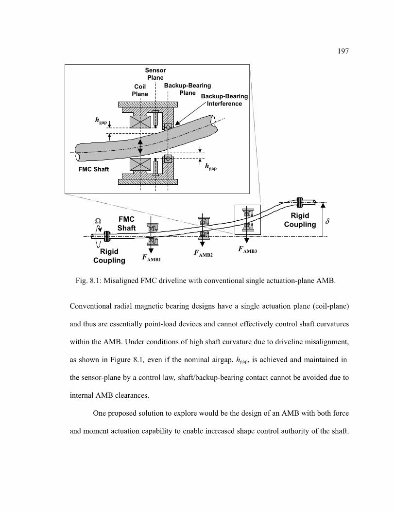
197

Conventional radial magnetic bearing designs have a single actuation plane (coil-plane)

and thus are essentially point-load devices and cannot effectively control shaft curvatures

within the AMB. Under conditions of high shaft curvature due to driveline misalignment,

as shown in Figure 8.1, even if the nominal airgap, hgap, is achieved and maintained in

the sensor-plane by a control law, shaft/backup-bearing contact cannot be avoided due to

internal AMB clearances.

One proposed solution to explore would be the design of an AMB with both force

and moment actuation capability to enable increased shape control authority of the shaft.

Backup-BearingPlane

Ω δRigid

Coupling

RigidCoupling

hgap

Backup-BearingInterference

Shaft

SensorPlane

hgapFMC Shaft

CoilPlane

FMCShaft

FAMB1FAMB2

FAMB3

Fig. 8.1: Misaligned FMC driveline with conventional single actuation-plane AMB.

198

This could be achieved with an additional coil-plane and sensor-plane within the

AMBs. See Figure 8.2.

This dual actuation plane AMB could reduce shaft curvature within the AMB and allow

the AMB-FMC driveline system to operate under more severe misalignment conditions

than with conventional single plane AMBs. In addition to shape control, the added

moment control authority could also increase the effectiveness of any vibration control

and potentially allow for fewer AMBs to be utilized in the overall control system. One

obvious design challenge would be to design the dual-plane AMB with minimal weight

and size increases over the single plane AMB design. Since the coils share the loading,

Backup-BearingPlane

hgap

FMC Shaft

BackPlane

FrontPlane

hgap

Ω

FAMB1

MAMB2

FAMB2

FAMB3

MAMB3

MAMB1 δRigid

Coupling

RigidCoupling

FMCShaft

Fig. 8.2: Misaligned FMC driveline with proposed dual actuation-plane AMB.

199

the size of coils in the dual-plane AMB device could be smaller than the coils of the

single plane AMB. Thus, with proper coil sizing, the size and mass of the dual plane

AMB could be close to the single plane AMB design. Furthermore, if the increased

modal control authority of the dual plane AMB enables fewer AMBs to be utilized, this is

also a potential weight saving benefit to be explored.

Another important issue raised by the Configuration II experimental investigation

is related to the rigid-coupling/FMC shaft attachment method and the coupling design.

Due to the low stiffness of the FMC shaft material, the conventional clamp-type rigid

couplings were not able to achieve sufficient clamping force to allow transmission of the

load-torque without slippage. Future investigations could explore new rigid-coupling

designs and FMC/coupling attachment methods to address this issue. In particular, future

investigations should focus on reversible (i.e. non-adhesive based) designs which would

allow repeated assembly and disassembly of FMC driveline system.

Finally, another important aspect of AMB-FMC drivelines which should be

investigated is in the area of system design. Previous researchers have conducted various

design studies for passive-bearing based, FMC and rigid matrix composite drivelines

based on tailoring the ply orientation angles and ply thickness, see Darlow, et al. (1990)

and Shin, et al. (2003). In these studies, significant weight savings over conventional

alloy shaft designs were achieved. Furthermore, in part, this thesis explores the use of

AMB technology with FMC driveshafts and develops a robust-adaptive vibration control

strategy for a given FMC shaft design. In order to take full advantage of the benefits

offered by an AMB-FMC driveline configuration, a simultaneous FMC structural

200

tailoring and active control law design needs to be performed. By combining the

adaptive control strategy and the corresponding robust design methodologies developed

in this thesis with a comprehensive FMC shaft design, an overall optimum AMB-FMC

design can be achieved. In the case of rotorcraft driveline systems, the minimum weight

AMB-FMC driveline design should be explored considering driveline torsional stiffness,

torsional bucking, maximum allowable misalignment, closed-loop robustness with

respect to FMC temperature sensitivity and required control power.

201

BIBLIOGRAPHY

Allaire, P. E., Humphris, R. R. and Barrett, L. E., 1986, "Critical Speeds and

Unbalance Response of a Flexible Rotor in Magnetic Bearings," Proceedings of the First

European Turbomachinery Symposium, London, Oct. 27-28, pp. 111-120.

Asokanthan, S. F. and Hwang, M. C., 1996, “Torsional Instabilities in a System

Incorporating a Hooke’s Joint,” Journal of Vibration Acoustics, Vol. 118, pp. 386-374.

Asokanthan, S. F. and Wang, X. H., 1996, “Characterization of Torsional

Instabilities in a Hooke’s Joint Driven System via Maximal Lyapunov Exponents,”

Journal of Sound and Vibration, Vol. 194, pp. 83-91.

Beer, F. P. and Johnston, E. R., Jr., 1992, Mechanics of Materials, 2nd Edition,

McGraw-Hill, Inc, New York.

Bolotin, V. V., 1963, Nonconservative Problems of the Theory of Elastic

Stability, Pergamon Press, New York.

Chen, L. W. and Chen, H. K., 1995, “Whirl Speed and Stability of Rotating Shaft

Subjected to End Loads,” AIAA Journal, Vol. 33, No. 9.

Chen, L. W. and Ku, D. M., 1990, “Dynamic Stability Analysis of A Rotating

Shaft By the Finite Element Method,” Journal of Sound and Vibration, Vol. 143, No. 1,

pp. 143-151.

Chen, L. W. and Ku, D. M., 1991, “Analysis of Whirl Speeds of Rotor-Bearing

Systems with Internal Damping by C0 Finite Elements,” Finite Elements in Analysis and

Design, Vol. 9, pp. 169-176.

202

Cohen, R. and Porat, I., 1984, “Influence of Load Torque on Stability of Rotor

Driven by Flexible Shaft,” Journal of Sound and Vibration, Vol. 95, pp. 151-160.

Cole, M. O. T., Keogh, P. S., and Burrows, C. R., 1998, “Vibration control of a

flexible rotor/magnetic bearing system subject to direct forcing and base motion

disturbances,” ImechE, Proceedings Journal (Part C), Vol. 212, pp. 535-546.

Cole, M. O. T., Keogh, P. S., and Burrows, C. R., 2000, “Adaptive-Q Control of

Vibration Due to Unknown Disturbances In Rotor/Magnetic Bearing Systems,” Proc. of

the 2000 IEEE International Conf. on Control Appls., Anchorage, Alaska, USA, Sept. 25-

27., pp. 965-970.

Darlow, M. S., Kraus, R. F. and Hetherington, P. L., 1990, “Demonstration of a

Supercritical Composite Helicopter Power Transmission Shaft,” Journal of the American

Helicopter Society, Vol. 35, No. 1, pp. 23-28.

DeSmidt, H. A., Wang, K. W. and Smith, E. C., 1998, “Active Vibration Control

of Rotorcraft Driveshaft-Airframe Dynamics,” Proceedings of the 54th American

Helicopter Society Annual Forum, Washington, D. C., May 20-22.

DeSmidt, H. A., Wang, K. W. and Smith, E. C., 2002, “Coupled Torsion-Lateral

Stability of A Shaft-Disk System Driven Through A Universal Joint,” ASME Journal of

Applied Mechanics, Vol. 69, No. 3, pp. 261-273.

Dewell, D. L. and Mitchell, L. D., 1984, “Detection of a Misaligned Disk

Coupling Using Spectrum Analysis,” Journal of Vibration, Acoustics, Stress, and

Reliability in Design, Vol. 106, pp. 9-16.

Dousis A. D., 1994, “Development and Integration of Onboard Drivetrain

Vibration Monitoring Systems,” Proceedings of the 50th American Helicopter Society

Annual Forum, Washington, D. C., May 11-13.

203

Dugundji, J. and Wendell, J. H., 1982, “Some Analysis Methods for Rotating

Systems with Periodic Coefficients,” AIAA Journal, Vol. 21, No. 6, pp. 890-897.

Eshleman, R. L. and Eubanks, R. A., 1969, “On the Critical Speeds of a

Continuous Rotor,” Transactions of the ASME, Journal of Engineering for Industry, pp.

1180-1188.

Friedmann, P. P., 1986, “Numerical Methods for Determining The Stability and

Response of Periodic Systems with Applications to Helicopter Rotor Dynamics and

Aeroelasticity,” Comp. and Maths. with Appls., Vol. 12A, No. 1, pp. 131-148.

Gangwani, S. T., 1981, “Calculation of Rotor Wake Induced Empennage

Airloads,” Presented at the American Helicopter Society National Specialists’ Meeting

on Helicopter Vibration, Technology for the Jet Smooth Ride, Hartford, Conn., Nov. 2-4.

Gibbons, C. B., 1980, “The Use of Diaphragm Couplings Turbomachinery,” Proc.

Mach. Vib. Monit. Ann. Sem., pp. 99-116.

Hartman. R. M., 1973, “A Dynamics Approach to Helicopter Transmission Noise

Reduction and Improved Reliability,” Proceedings of the 29th American Helicopter

Society Annual Forum.

Horn, J., Calise, A. J. and Prasad J. V. R., 2002, “Flight Envelope Limit Detection

and Avoidance for Rotorcraft,” Journal of the American Helicopter Society, Vol. 47, No.

4, pp. 253-262.

Hsu, C. S., 1963, “On the Parametric Excitation of a Dynamic System Having

Multiple Degrees of Freedom,” ASME Journal of Applied Mechanics, Vol. 30, pp. 367-

372.

Hsu, C. S., 1965, “Further Results on Parametric Excitation of a Dynamic

System,” ASME Journal of Applied Mechanics, Vol. 32, pp. 373-377.

204

Humphris, R. R., Kelm, R. D., Lewis, D. W. and Allaire, P. E., 1986, “Effect

of Control Algorithms on Magnetic Journal Bearing Properties,” ASME Paper No. 86-

GT-54.

Inman, D. J., 1994, Engineering Vibration, Prentice Hall, New Jersey.

Iwatsubo, T. and Saigo, M., 1984, “Transverse Vibration of a Rotor System

Driven by a Cardan Joint,” Journal of Sound and Vibration, Vol. 95, pp. 9-18.

Jones, R.M., 1975, Mechanics of Composite Materials, McGraw-Hill, New York.

Kasarda, M. E., Clements, J., Wicks, A. L., Hall, C. D., and Kirk, R. G., 2000,

“Effect of Sinusoidal Base Motion on a Magnetic Bearing,” Proc. of the 2000 IEEE

International Conf. on Control Appls., Anchorage, Alaska, USA, Sept. 25-27., pp. 144-

149.

Kato, M. and Ota, H., 1990, “Lateral Excitation of a Rotating Shaft Driven by a

Universal Joint with Friction,” Journal of Vibration and Acoustics, Vol. 112, pp. 298-

303.

Khader, N., 1997, “Stability Analysis for the Dynamic Design of Rotors,” Journal

of Sound and Vibration, Vol. 207, pp. 287-299.

Kirk, R. G., Mondy, R. E. and Murphy, R. C., 1984, “Theory and Guidelines to

Proper Coupling Design for Rotor Dynamics Considerations,” Journal of Vibration,

Acoustics, Stress, and Reliability in Design, Vol. 106, pp. 129-138.

Knospe, C.R., Hope, R.W., Fedigan, S.J. and Williams, R.D., 1993, “Adaptive

On-Line Balancing Using Digitial Control,” Proc. Mag ‘93: Magnetic Bearings,

Magnetic Drives and Dry Gas Seals Conference and Exhibition, pp. 153-164.

Knospe, C.R., Hope, R.W., Fedigan, S.J. and Williams, R.D., 1995, “Experiments

in the Control of Unbalance Response using Magnetic Bearings,” Mechatronics, pp. 385-

400

205

Knospe, C.R., Tamer, S.M. and Fedigan, S.J., 1997, “Robustness of Adaptive

Rotor Vibration Control to Structured Uncertainty,” Journal of Dynamic Systems

Measurement and Control, pp. 243-250.

Kraus, R. F. and Darlow, M. S., 1987, “Design and Experimental Studies of

Composite Power Transmission Shafting," Proceedings of the 43rd American Helicopter

Society Annual Forum, St. Louis, Mo.

Lee, C. W. and Yun, J. S., 1996, “Dynamic Analysis of Flexible Rotors Subjected

to Torque and Force,” Journal of Sound and Vibration, Vol. 192, pp. 439-452.

Lee, H. P., Tan, T. H. and Leng, G. S. B., 1997, “Dynamic Stability of Spinning

Timoshenko Shafts With A Time-Dependent Spin Rate,” Journal of Sound and Vibration,

Vol. 199, pp. 401-415.

Leishman, J. G. and Bi, N., 1989, “Aerodynamic Interactions Between a Rotor

and a Fuselage in Forward Flight,” Proceedings of the 45th American Helicopter Society

Annual Forum, Boston, Mass., May 22-24.

Lewis, S. A., 1994, Sliding Mode Control of a Flexible Rotor via Magnetic

Bearings: Theory and Experiments, Ph.D. Thesis, The Pennsylvania State University.

Lin, C., Wang, J., and Yang, G. H., 1999, “H∞ Control for a Class of Descriptor

Systems with Uncertainties in the Derivative Matrix,” Proceedings of the American

Control Conference, San Diego, California, pp. 3382-3386.

Mancuso, J. R., 1986, “Disc vs. Diaphragm Couplings,” Machine Design, Vol.

58, No. 17, pp. 95-98.

Mancuso, J. R., 1986, Coupling and Joints: Design, Selection, and Application,

Marcel Dekker, Inc., New York, ISBN 0-8247-7400-0.

206

Mazzei, A. J., Jr., Argento, A. and Scott, R. A., 1999, “Dynamic Stability of a

Rotating Shaft Driven through a Universal Joint,” Journal of Sound and Vibration, Vol.

222, pp. 19-47.

Mease, K., 1991, Sliding Mode Control of a Rigid Rotor: Theory and

Experiments, Master’s Thesis, The Pennsylvania State University.

Meeks, C. D. and Spencer, V., 1990, "Development of a Compact, Light Weight

Magnetic Bearing,"ASME Paper No. 90-GT-240.

Meirovitch, L., 1980, Computational methods in structural dynamics, Sijthoff &

Noordhoff, The Netherlands.

Nikolajsen, J. L., Holmes, R., and Gondhalekar, V., “Investigation of an

Electromagnetic Damper for Vibration Control of a Flexible Transmission Shaft,”

ImechE, Vol. 193, No. 31, 1979, pp. 331-336.

Nonami, K., 1988, "Vibration and Control of Flexible Rotor Supported by

Magnetic Bearings," Magnetic Bearings, (G. Schweitzer, Editor), Springer-Verlag, pp.

177-186.

Nonami, K. and Takayuki, I., 1996, “µ Synthesis of Flexible Rotor-Magnetic

Bearing Systems,” IEEE Transactions on Control Systems Technology, Vol. 4, No. 5, pp.

503-512.

Norman, R. T. and Yamauchi, G. K., 1991, “Full-Scale Investigation of

Aerodynamic Interactions Between A Rotor and Fuselage,” Proceedings of the 47th

American Helicopter Society Annual Forum, Phoenix, Arizona, May.

Ocalan, M., 2002, High Flexibility Rotorcraft Driveshafts Using Flexible Matrix

Composites and Active Bearing Control, Master’s Thesis, The Pennsylvania State

University.

207

Okada, Y. Nagai, B., and Shimane, T., 1988, “Digital Control of Magnetic

Bearing with Rotationally Synchronized Interruption,” Magnetic Bearings (G Schweitzer,

Editor), Springer-Verlag, New York, pp. 357-364.

Oppenheim, A. V. and Schafer, R. W., 1989, Discrete-Time Signal Processing,

Prentice-Hall, Inc., Englewood Cliffs, NJ.

Rosenberg, R. M. and Ohio, T., 1958, “On the Dynamical Behavior of Rotating

Shafts Driven by Universal (Hooke) Coupling,” ASME Journal of Applied Mechanics,

Vol. 25, pp. 47-51.

Ryu, J. H., Kwon, D. S. and Park, Y., 1999, “A Robust Controller Design Method

for a Flexible Manipulator with a Time Varying Payload and Parameter Uncertainties,”

Proceedings of the IEEE International Conference on Robotics and Automation, Detroit,

Michigan, May, pp. 413-418.

Saigo, M., Okada, Y. and Ono, K., 1997, “Self-excited Vibration Caused by

Internal Friction in Universal Joints and Its Stabilizing Method,” Journal of Vibration and

Acoustics Vol. 119, pp. 221-229.

Salm, J. R. and Schweitzer, G., 1984, "Modeling and Control of Flexible Rotor

with Magnetic Bearings," ImechE, pp. 553-559.

Shan, Y. and Bakis, C. E., 2002, “Static and Dynamic Characterization of a

Flexible Matrix Composite Material,” Proceedings of the 58th American Helicopter

Society Annual Forum, Montreal, Quebec, June 11-13.

Shan, Y. and Bakis, C. E., 2003, “Frequency and Temperature Dependent

Damping Behavior of Flexible Matrix Composite Tubes,” 35th International SAMPE

Technical Conference, September 28 -October 2, Dayton, OH.

208

Sheu, P. P., Chieng, W. H. and Lee, A. C., 1996, “Modeling and Analysis of

the Intermediate Shaft Between two Universal Joints,” Journal of Vibration and

Acoustics, Vol. 118, pp. 88-99.

Sinha, A., 1990, “On the Design of Magnetic Suspension Systems,” ASME Paper

No. 90-GT-239.

Shin, E., Wang, K. W., and Smith, E., 2003, “Characterization of Flexible Matrix

Composite Rotorcraft Driveshafts,” Proc. 59th Forum, American Helicopter Society,

Mesa, AZ.

Sinha, A. and Miller, D. W., 1995, “Optimal Sliding Mode Control of A Flexible

Spacecraft Under Stochastic Disturbances,” AIAA Journal of Guidance, Dynamics and

Control, Vol. 18, No. 3, pp. 486-492.

Sinha, A., Wang, K. W. and Mease, K. L., 1991, “Robust and Real-Time Rotor

Control with Magnetic Bearings,” Proceedings of the AIAA/NASA/OAI conference on

advanced SEI Technology, Columbus, Ohio, Sept. 4-6.

Sivrioglu, S. and Nonami, K., 1996, “LMI Approach to Gain Scheduled H∞

Control beyond PID Control for Gyroscopic Rotor-Magnetic bearing System,” Proc. of

the 35th Conf. on Decision and Control, Kobe, Japan, Dec., pp. 3694-3699.

Stanway, R. and Burrows, C. R. 1981, “Active Vibration Control of a Flexible

Rotor on Flexibly-Mounted Journal Bearings,” ASME Journal of Dynamic Systems,

Measurement and Control, Vol. 103, pp. 383-388.

Suzuki, Y., 1998, “Acceleration feed-forward control for active magnetic bearing

systems excited by ground motion,” IEE Proc.-Control Theory Appl., Vol. 145, No. 2,

pp. 113-118.

Tay, T. T. and Moore, J. B., 1991, “Enhancement of fixed controllers via

adaptive-Q disturbance estimate feedback,” Automatica, Vol. 27, pp. 39-53.

209

Toossi, M. and Callahan, C. B., 1994, “Determination of AH-64 Airframe In-

Flight Modal Frequencies Using Rotor Control-Induced Excitations,” Proceedings of the

50th American Helicopter Society Annual Forum, Washington, D. C., May 11-13.

Toossi, M., Callahan, C. B. and Santee, J. E., 1994, “Using Resilient Connections

for Helicopter Airframe Modal Frequency Placement,” Proceedings of the 50th American

Helicopter Society Annual Forum, Washington, D. C., May 11-13.

Utkin, V., 1977, “Variable Structure Systems with Sliding Modes,” IEEE

Transactions on Automatic Control, Vol. AC-22, pp. 212-222.

Vance, J. M., 1988, Rotordynamics of Turbomachinery, John Wiley and Sons,

New York.

Wereley, N.M. and Hall, S.R., 1990, “Frequency Response of Linear Time

Periodic Systems,” Proceedings of 29th IEEE Conference on Decision and Control,

Honolulu, Hawaii, pp. 3650-3655.

Wu, W. T., Griffin, J. H. and Wickert, J. A., 1995, “Perturbation Method For the

Floquet Eigenvalues and Stability Boundary of Periodic Linear Systems,” Journal of

Sound and Vibration, Vol. 182, pp. 245-257.

Xu, M. and Marangoni, R. D., 1990, “Flexible Couplings: Study and

Application,” Shock and Vibration Digest, Vol. 22, pp. 3-11.

Xu, M. and Marangoni, R. D., 1994, ”Vibration Analysis of a Motor-Flexible

Coupling-Rotor System Subjected to Misalignment and Unbalance. Part I: Theoretical

Model and Analysis,” Journal of Sound and Vibration, Vol. 176, pp. 663-679.

Xu, M. and Marangoni, R. D., 1994, ”Vibration Analysis of a Motor-Flexible

Coupling-Rotor System Subjected to Misalignment and Unbalance. Part II: Experimental

Validation,” Journal of Sound and Vibration, Vol. 176, pp. 681-691.

210

Yim, K. B., Noah, S. T. and Vance, J. M., 1986, “Effect of Tangential Torque

on the Dynamics of Flexible Rotors,” ASME Trans., Journal of Applied Mechanics, Vol.

53, pp. 711-718.

Zhou, K., Doyle, J., and Glover, K., 1996, Robust and Optimal Control, Prentice-

Hall, New York.

Zorzi, E. S. and Nelson, H. D., 1977, “Finite Element Simulation of Rotor-

Bearing Systems With Internal Damping,” ASME Trans., Journal of Engineering for

Power, Vol. 99, pp. 71-76.

Zorzi, E. S. and Nelson, H. D., 1979, “The Dynamics of Rotor-Bearing Systems

With Axial Torque-A Finite Element Approach,” ASME Paper No. 79-DET-68.

211

Appendix A

FINITE ELEMENT MODEL ELEMENTAL MATRICES

A.1 Shaft Elemental Matrices

The ith shaft inertia matrix of the jth element for ]2 ,1[=i and ], , 2, 1[ ielNj L= is

[ ]∫ +′′+′′+++=ielL T

swT

wvT

vswTwv

Tvu

Tus

ijel dxNNJmNNNNImNNNNNNm

0, )()( φφM ( A.1 )

The ith shaft gyroscopic matrix of the jth element for ]2 ,1[=i and ], , 2, 1[ ielNj L= is

dxNNNNJmielL

vT

wwT

visi

jel ∫ ′′−′′Ω=0

, )(G ( A.2 )

The ith shaft damping matrix of the jth element for ]2 ,1[=i and ], , 2, 1[ ielNj L= is

[ ]∫ ′′+′′′′+′′′′+′′=ielL T

sswT

wvT

vssuT

usssi

jel dxNNJGNNNNIENNAE0

, )( φφξC ( A.3 )

The ith shaft elastic stiffness matrix of the jth element for ]2 ,1[=i and ], , 2, 1[ ielNj L= is

212

( )[ ]∫ ′′+′′′′+′′′′+′′=ielL T

sswT

wvT

vssuT

ussi

jel dxNNJGNNNNIENNAE0

, φφK ( A.4 )

The ith shaft rotational-damping stiffness matrix of the jth element for ]2 ,1[=i and

], , 2, 1[ ielNj L= is

∫ ′′′′−′′′′Ω=ielL

vT

wwT

visssi

jel dxNNNNIE0, )(ξrdK ( A.5 )

The ith shaft axial-buckling stiffness matrix of the jth element for ]2 ,1[=i and

], , 2, 1[ ielNj L= is

∫ ′′+′′−=ielL

wT

wvT

vai

jel dxNNNNP0, )(PK ( A.6 )

The ith shaft torque-buckling stiffness matrix of the jth element for ]2 ,1[=i and

], , 2, 1[ ielNj L= is

∫ ′′′−′′′=ielL

vT

wwT

vLi

jel dxNNNNT0, )(TK ( A.7 )

A.2 Fuselage-Beam Elemental Matrices

The fuselage-beam inertia matrix of the jth element for ], , 2, 1[ felNj L= is

213

[ ] )(0 112233, ∫ +′′+′′+++=

felL T

fwT

wfvT

vfwTwv

Tvu

Tuf

fjel dxNNImNNImNNImNNNNNNm φφM ( A.8 )

The fuselage-beam damping matrix of the jth element for ], , 2, 1[ felNj L= is

[ ]∫ ′′+′′′′+′′′′+′′=f

elL Tcsffw

Twffv

Tvffu

Tufff

fjel dxNNJGNNIENNIENNAE

0 2233, φφξC ( A.9 )

The fuselage-beam elastic stiffness matrix of the jth element for ], , 2, 1[ felNj L= is

[ ]∫ ′′+′′′′+′′′′+′′=felL T

csffwT

wffvT

vffuT

ufff

jel dxNNJGNNIENNIENNAE0 2233, φφK ( A.10 )

214

Appendix B

MISALIGNMENT-INDUCED INERTIA LOAD AND TORQUE LOAD

PERIODIC NCV COUPLING TERMS

B.1 Load-Inertia NCV Terms

The kinetic energy of the torsional inertia load, JL , is

221

LLLJ JT Ω= ( B.1 )

Time differentiation of (2.12), gives the load rotation speed, dtd L

Lφ

=Ω , which is a

function of the static misalignments and twists, [ ]sCsBABC φφγγξξδδθ 323232= , and

shaft elastic slopes and twists, [ ] TCCCBBBBBAAABC wvwvwvwvq ,2,2,2,2,2,1,1,1,1,1ˆ--ˆ-- φφ ′′′′′′′′= ,

at couplings A, B and C. Functionally, LΩ is written as

),,,,( 0 tqq ABCABCABCLL &θΩΩ=Ω ( B.2 )

where ABCq is related to the global unconstrained generalized coordinate vector, q, via

the transformation qqABC abcT= . According to Lagrange’s Equations, the contribution of

the torsional load-inertia kinetic energy to the equations-of-motion is

215

∂Ω∂

Ω+

∂Ω∂

−

∂Ω∂

Ω=

∂Ω∂

−

∂Ω∂

Ω+∂Ω∂

Ω=∂

∂−

∂

∂

ABC

LLL

ABC

L

ABC

LLL

T

LLLL

LLL

LJLJ

qJ

qqdtdJ

qqdtdJ

qJ

qT

qT

dtd

&&

&L

&&&

&

abcT ( B.3 )

with

0=∂Ω∂

−

∂Ω∂

ABC

L

ABC

Lqqdt

d&

( B.4 )

and

[ ][ ]

[ ][ ])2cos()2sin(

)2cos()2sin(

)2cos()2sin(

)2cos()2sin(

00

00

00

00

tt

qtt

qtt

qttq

J

ABC

ABC

ABCABC

LLL

Ω+Ω+−

Ω+Ω++

Ω+Ω++

Ω+Ω+≡∂Ω∂

Ω

∆∆∆

∆∆∆

∆∆∆

∆∆∆

c2s20

c2s20

c2s20

c2s20

fff

kkk

ccc

mmm

L

L

&L

&&&

&

( B.5 )

Where the inertia coupling matrices are given by (B.6) – (B.8).

216

...( B.6 )

...

217

( B.7 )

...

218

( B.8 )

The damping coupling matrices are given by (B.9) – (B.11).

219

... ( B.9 )

...

220

( B.10 )

...

221

( B.11 )

The stiffness coupling matrices are given by (B.12) – (B.14).

222

... ...

( B.12 )

223

( B.13 )

224

( B.14 )

The forcing terms are given by (B.15) – (B.17).

225

+++

+++++++

++++

+++

Ω=

Σ∆∆

Σ∆∆

∆Σ∆

∆Σ∆

∆Σ∆

∆Σ∆

∆∆Σ

∆∆Σ

∆

0) - (2 ) -() - -( ) - (2-) (2 ) - () ( )(2-

0) (2 - )-(- ) - - (- ) (2 ) - (2 - ) - (-) - ( ) - (2

4

32323222

2

222332322

32323222

2

222332322

32323222

2

222332322

32323222

2

222332322

20

0

ξξδδγγξδγγξδγξξδδγγγδδξγξδξγξδξγγδδξ

γγδδξγξδξγξδξγγδδξξξγγδγξδδγξδδξξγγδ

LJf ( B.15 )

+

+

+

+

+

+

+

+

+

Ω=

∆∆∆

∆∆∆

∆∆∆

∆∆∆

∆∆∆

∆∆∆

∆∆∆

∆∆∆

∆∆∆

∆

) - 4(- - -

) - (-

) - (-

) - (-

) - (-0

) - (-

) - (-

) - (-

) - (-

3232222

22232

1

22222

1

22232

1

22222

1

22232

1

22222

1

22232

1

22222

1

202

γγφξξφγξδ

γξδγ

γξδγ

γξδξ

γξδξ

γξδξ

γξδξ

γξδδ

γξδδ

sCsB

LJsf ( B.16 )

++++++

++++

Ω=

∆∆

∆

) - - 2(-) - (-) - (-) - (-) - (-

0) - (-) - (-) - (-) - (-

22323232

3232323323232232323233232322

3232323323232232323233232322

20

γφξφγγξξδδγγξξδδγγγξξδδγγγξξδδξγγξξδδξ

γγξξδδξγγξξδδξγγξξδδδγγξξδδδ

sCsB

LJc2f ( B.17 )

With the definitions

226

23

22

223

22

2

23

22

223

22

2

23

22

223

22

2

,

,

,

γγγγγγ

ξξξξξξ

δδδδδδ

−=+=

−=+=

−=+=

∆Σ

∆Σ

∆Σ

( B.18 )

Finally, the load-inertia NCV coupling matrices and forcing terms in global

unconstrained coordinates are

[ ][ ][ ][ ])2cos()2sin()(

)2cos()2sin()(

)2cos()2sin()(

)2cos()2sin()(

00

00

00

00

ttt

ttt

ttt

ttt

T

T

T

T

Ω+Ω+=

Ω+Ω+=

Ω+Ω+=

Ω+Ω+=

∆∆∆∆

∆∆∆∆

∆∆∆∆

∆∆∆∆

c2s20abc

abcc2s20abc

abcc2s20abc

abcc2s20abc

fffTF

TkkkTK

TcccTC

TmmmTM

( B.19 )

B.2 Load-Torque NCV Terms

In (2.58), the load-torque NCV terms are given as the generalized force vector LTQ ,2 ,

which is

qTQ LLLT ∂∂

−=φ

,2 ( B.20 )

Since the load rotation angle, Lφ , is functional represented as

),,,( 0 tqABCABCLL θφφφ = ( B.21 )

LTQ ,2 becomes

∂∂

−=∂∂

−=∂∂

−=ABC

LL

T

ABC

LTL

LLLT q

Tq

Tq

TQ φφφabcabc TT,2 ( B.22 )

with (B.23)

227

Ω+Ω+−

Ω+Ω+≡

∂∂

ΓΓΓ

ΓΓΓ

)2cos()2sin(

)2cos()2sin(

00

00

tt

qttq

T ABCABC

LL

c2s20

c2s20

fff

kkk

L

φ

( B.23 )

Where the stiffness coupling matrices are given by (B.24) – ( B.26).

=Γ

0000000000000000000000000000000000000-000000000000000000000000000000000-00000000000000000000000000

21

21

21

21

LT0k ( B.24 )

−=Γ

0-0000000--0000000

--0000000000--00000--00000-0-00000---00000--0000000000-0000000000

32

321

221

21

321

21

221

323221

321

21

221

21

21

γγγφγφ

φξφφξφξξξξ

φξφφξφ

sC

sC

sBsB

sBsB

sBsB

sBsB

LTs2k ( B.25 )

228

=Γ

0--0000000--0000000-0000000000---00000---00000--000000--00000--00000000000000000000

23

221

321

21

221

21

321

232321

221

21

321

21

21

γγγφγφ

φξφφξφ

ξξξξφξφ

φξφ

sC

sC

sBsB

sBsB

sBsB

sBsB

LTc2k ( B.26)

And the forcing terms are given by (B.27).

=Γ

0

02

-

3232

3232

γγξξ

ξξδδ

LT0f ,

+

+

+

=Γ

3232233223

323223

23

2-2-22-2

22-2--

--

2

γγγφγγφγξφξξφξ

ξξξφξξφξ

δδ

sCsCsBsB

sBsB

LTs2f , and

+++++=Γ

23

22

2332

2332

23

22

2332

32

-22-22-

-2--2--

2

γγγφγγφγξφξξφξ

ξξξφξξφξ

δδ

sCsCsBsB

sBsB

LTc2f ( B.27 )

Finally, the load-torque NCV coupling matrices and forcing terms in global

unconstrained coordinates are

[ ][ ])2cos()2sin()(

)2cos()2sin()(

00

00

ttt

tttT

T

Ω+Ω+=

Ω+Ω+=

ΓΓΓΓ

ΓΓΓΓ

c2s20abc

abcc2s20abc

fffTF

TkkkTK( B.28 )

229

Appendix C

NON-DIMENSIONAL SYSTEM MATRICES FOR CONVENTIONAL

DRIVELINE

C.1 Non-Dimensional Nominal System Matrices

The non-dimensional (N.D.) nominal mass and gyroscopic matrices, M and G , are

=

100000000010000000001000000000100000000010000000001000000000100000000010000000001

M and

−

−

−

−

=

0000000000000000000000000000000000000000000000000000000000000000000000000

8

22

22

11

11

22

0

ff

ff

ff

ff

f πεG (C.1)

The N.D. structural and auxiliary damping matrix, sdC and auxC , are

=

φφ ζζ

ζζ

ζζ

ζζ

ζ

ff

ff

ff

ff

f

000000000000000000000000000000000000000000000000000000000000000000000000

2

2222

2222

1111

1111

sdC (C.2)

and

230

=

000000000

000000000

000000000

000000000

000000000

00000000

00000000

00000000

00000000

d

d

d

d

c

c

c

c

auxC (C.3)

Finally, the N.D. elastic and rotating-frame-damping stiffness matrices, K and rdK , are

=

2

22

22

22

22

21

21

21

21

000000000000000000000000000000000000000000000000000000000000000000000000

φff

ff

ff

ff

f

K (C.4)

and

−

−

−

−

=

0000000000000000000000000000000000000000000000000000000000000000000000000

2

2222

2222

1111

1111

0

ζζ

ζζ

ζζ

ζζ

ff

ff

ff

ff

frdK (C.5)

C.2 Non-Dimensional Load-Inertia NCV Terms

The N.D. inertia coupling matrices are given by (C.6) – (C.8).

231

=∆

0000-0

00-0-0-0

0300-0

0-0000

0030-0

0-0000

-0-0-00-

0-0000

000-0

2 2

22

2

2

22

232

22

22

22

223

2

2

2

4

2 4

2

2

232

4

234

2

22

4

42

2

2

223

4

423

2

µπγ

µπδ

µπγ

µπδ

γγδπγγγδ

γδδπδγδδ

γγδγγδπγγγδγγδ

γδδγδδπδγδδγδδ

γδγ

γδγ

δγδ

δγδµπ0M (C.6)

=∆

0--0--0

02020-0

-202-0-0-0

-02-02-00-0202-0-0-0

-0-0-00-

-0000

-0-0-00-

00-0-0-0

2422

22

222

22

222

22

2

2

22

2

2

22

222

222

2

2

µπγ

µπγφ

µπδ

µπγ

µπγφ

µπδ

πγπγφπδ

πγγδγπγφγδγπδδγδ

δγδ

γδγγδγ

γδγγδγ

δγδδγδδγδδγδ

γδγ

γδγ

δγδ

δγδ

µπ

ss

s

s

s2M (C.7)

=∆

2

24222

2

22

22

222

222

2

-0---0-

00000000

040002-00000000000

-0004-0002-

-00000000

-02-00000000000000

-0002-000-

µπ

γµπγφ

µπγ

µπδ

µπγφ

µπγ

µπδ

πγφπγ

πδπγφπγ

πδ

γγ

δδ

γγ

δδ

µπ

ss

s

s

c2M (C.8)

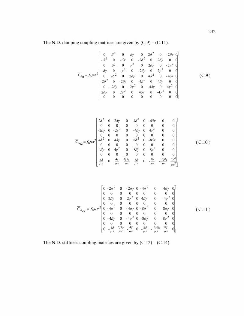
232

The N.D. damping coupling matrices are given by (C.9) – (C.11).

=∆

000000000004-0402020404-02-02-000404-02-02-04-040202000202-0-0-02-0200000202-0-0-02-02000

22

22

22

22

22

22

22

22

20

γδγγδγγδγγδγ


γδγγδγγδγγδγ


µπf0C (C.9)

=∆

2

221688844

22

22

22

22

20

--00

000000000008-080404000000000008-08040400000000000404-02-02-000000000004-040202

µπ

γµπγφ

µπγ

µπδ

µπγφ

µπγ

µπδ

γδγγδγ

δγδδγδ

γδγγδγ

δγδδγδ

µπ

ss

fs2C ( C.10 )

=∆

0--0--00000000000808-04-04-00000000000808-04-04-000000000004-04020200000000000404-02-02-0

8s168484

22

22

22

22

20

µπγ

µπγφ

µπδ

µπγ

µπγφ

µπδ

γδγγδγ

δγδδγδ

γδγγδγ

δγδδγδ

µπ

s

fc2C ( C.11 )

The N.D. stiffness coupling matrices are given by (C.12) – (C.14).

233

( )( )

( )( )

( )( )

( )( )

++−

+−

−

+

−

+

=∆

00004200

02-0--02-4-0

002

-00

0-0-

0-0

0-0-

222

22

222

22

2221

2221

2212

2212

220

γδγδδγδ

γδγδγδγ

γγδ

γγδ

γδδ

γδδ

µπf0K ...

( )( )

( )( )

( )( )

( )( )

−+

−+

++−

+−

0000004-02-0004-0202-04-000204-0420-0002-0002-4-000-02

22

22

22

22

222

22

222

22

γγδγγδ

γδδγδδ

γδγδδγδ

γδγδγδγ

( C.12 )

( )

( )

( )

( )

++

++

+−

+−

=∆

µπγ

µπγφ

µπδ

γδγγδ

γδγδδ

γδγγδ

γδγδδ

µπ

484

22

22

22

22

22

22

22

22

220

-0000)(2-

40200)(2-00

2040000)(-

2-00000

-020

s

fs2K ...

( )

( )

( )

( )

+−

+−

++

++

0-00000)(408-04-000)(4-00040800000)(20402-000)(20002-040

8168

22

22

22

22

22

22

22

22

µπγ

µπγφ

µπδ

γδγγδ

γδγδδ

γδγγδ

γδγδδ

s

( C.13 )

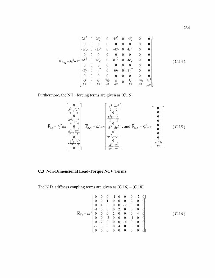
234

=∆

2

22s1688844

22

22

22

22

220

--00

000000000008-080404000000000008-08040400000000000404-02-02-000000000004-040202

µπ

γµπγφ

µπγ

µπδ

µπγφ

µπγ

µπδ

γδγγδγ

δγδδγδ

γδγγδγ

δγδδγδ

µπ

s

fc2K ( C.14 )

Furthermore, the N.D. forcing terms are given as (C.15)

+

+

+

=∆

0--

0

0

0

0

2

3

2

2

2

2

23

4

3

4

2

4

2

43

20

γγδ

δγδ

γγδ

δγδ

µπf0F ,

+

=∆

µπγ

µπδ

γγδ

δγδ

γγδ

δγδµπ

22

32

23

2

3

2

2

2

2

23

20

--

0--

0--0

0--

fs2F , and

=∆

µπφγ

µπ

s

f

22

20

-

00000000

c2F ( C.15 )

C.3 Non-Dimensional Load-Torque NCV Terms

The N.D. stiffness coupling terms are given as (C.16) – (C.18).

=Γ

000000000000040002-0004-00020004-0002-00040002000000020001-0002-000100020001000-2000-1000

2τπ0K ( C.16 )

235

=Γ

00-000000044-446-22-

-40446-4-2-2-04-404-2-24-20444-02224046-2-201-

6-4-220-1-022-4-21-0-02-2-24-1--0

42

2

2

µπγ

µπγ

πγ

πγ

φφφφφφφφ

φφφφφφφφ

φφφφφφφφ

φφφφφφφφ

τπ

ssss

ssss

ssssssss

ssss

ssss

ssssssss

s2K ( C.17 )

=Γ

0000-000

4-04-4-64220044-446-22-04-4-402-2-2-4-04-404-2-24-2

-642-2--01046-2-201-0222-4-1002-2-421-0-

42

2

2

µπγ

µπγ

πγ

πγ

φφφφφφφφ

φφφφφφφφ

φφφφφφφφ

φφφφφφφφ

τπ

ssss

ssssssss

ssss

ssss

ssssssss

ssss

c2K ( C.18 )

Finally, the N.D. forcing terms are given as (C.19)

+

=Γ

00-0--

0--

0-

22

22

γδ

γδτπ

γδ

γδ

0F ,

+

+

+

+

=Γ

µπφγ

γδ

γδ

γφγδγφγφγδ

γφγφ

γφγφ

γφ

τπ

s

s

ss

s

s

s

s

2

2

2

222

222

s

-

2--2

2-2

-

--

s2F and

+

+

+

+

=Γ

µπγ

γδ

γδ

γφγφγδ

γφγφγδ

γφγφ

γφγφ

τπ

2

2s

2s

s

2s

s

2s22

s

2s22

2-2--

2-2-

--

-

c2F ( C.19 )

236

Appendix D

LEAST-SQUARES FORMULATION OF ADAPTIVE CONTROL UPDATE LAW

Given the transfer matrix nnyuT

×ℜ∈ from the control input to the response output

Fourier coefficient vectors, 1 ×ℜ∈ nU and 1 ×ℜ∈ nY , and given the baseline system response

1 ×ℜ∈ nbY , the system steady-state response is given by

byu YUTY += ( D.1 )

If the control input U is updated at each time interval i, the steady state relation is written

biyui YUTY += ( D.2 )

Where Yi is the steady-state response to the ith control update Ui. The update law for Ui

can be obtained through minimization of the quadratic objective function Ji given as

iTii

Tii RUUWYYJ += ( D.3 )

Where TWW = and TRR = are symmetric, positive definite, weighting matrices. By using

the fact that

biyui YUTY += −− 11 ( D.4 )

iY can be written in terms iU , 1−iU and 1−iY as

1−+∆= iiyui YUTY with 1−−=∆ iii UUU ( D.5 )

Substituting (D.5) into (D.3 ), the objective function is expressed as

237

iTiiiyu

T

iiyui RUUYUTWYUTJ +

+∆

+∆= −− 11 ( D.6 )

Since Ji is quadratic with Ji ≥ 0, the control input Ui that minimizes Ji satisfies

iT

iiTT

yuiT

yuiyuTT

yuiyuT

yui

i URRUYWTWYTUTWTUWTTUJ

++++∆+∆==∂∂

−− 110 ( D.7 )

Since TWW = and TRR = and 1−−=∆ iii UUU (D.7) becomes

iiT

yuiiyuT

yu RUWYTUUWTT ++−= −− 11)(0 ( D.8 )

Solving for Ui the control update law becomes

−

+= −−

−

11

1

iiyuT

yuyuT

yui YUTWTRWTTU ( D.9 )

Or, in terms of the indices i and i+1 the control update law is

−

+=

−

+ iiyuT

yuyuT

yui YUTWTRWTTU1

1 ( D.10 )

238

Appendix E

ADAPTIVE CONTROL CONVERGENCE CONDITION

Given the Fourier coefficient transfer matrix nnyuT ×ℜ∈ and the baseline system

response vector 1 ×ℜ∈ nbY , the steady-state response 1 ×ℜ∈ n

iY to the ith updated control input

1 ×ℜ∈ niU is

biyui YUTY += (E.1)

Also, given the control update law based on an estimate of the Fourier coefficient transfer

matrix nnyuT ˆ ×ℜ∈ , the control update law is

−

+=

−

+ iiyuT

yuyuT

yui YUTWTRTWTU ˆˆˆˆ1

1 (E.2)

Substituting the expression for iY in (E.1) into the update law in (E.2), the recursion

relation of the control input iU is expressed as

bii QYPUU +=+1 (E.3)

With matrices P and Q defined as

WTRTWTQ

TTWTRTWTP

Tyuyu

Tyu

yuyuT

yuyuT

yu

ˆˆˆ

ˆˆˆˆ

1

1

−

−

+−=

−

+=

(E.4)

239

Since Yb is a constant vector, the stability of the above discrete-time system only

depends on the eigenvalues of the mapping matrix, P, from Ui to Ui+1. Specifically, the

stability condition of (E.3) is

able Unst1][

Stable 1][

≥

<

P

P

ρ

ρ(E.5)

Where ] [ρ is the spectral radius. If (E.3) is stable then update law in (E.2) is said to

converge, otherwise the update law it is said to diverge.

Assuming the update law (E.2) converges, then cii UUU →→ +1 as ∞→i where Uc

is the converged control input vector. Substituting Uc for Ui and Ui+1 into (E.3) and

solving for Uc

bc QYPIU 1)( −−= (E.6)

Furthermore substituting Uc for Ui in the expression for Yi in (E.1), the converged output

response cii YYY →→ +1 with ∞→i is expressed as

bbyuc YQYPITY +−= −1)( (E.7)

Finally, substituting the expressions for matrices P and Q defined in (E.4) into (E.6) and

(E.7), the converged control input and response vectors become

bbT

yuyuT

yuyuc

bT

yuyuT

yuc

YWYTRWTTTY

WYTRWTTU

++−=

+−=

−

−

ˆ]ˆ[

ˆ]ˆ[

1

1

(E.8)

240

Appendix F

FMC SHAFT LAYUP AND EQUIVALENT MATERIAL PROPERTIES

The FMC shaft considered in this investigation is based on a symmetric ply layup

configuration where the fiber orientations are wound in +θi and –θ i directions for each

specified ply orientation angle θi. Here θi is the fiber angle relative to the shaft axis.

Figure F.1 is a schematic of the FMC composite shaft and Figure F.2 gives the layer

locations, zk, through the shaft wall thickness relative the laminate mid-plane.

θi

Fig. F.1: FMC shaft with in-plane force resultants.

241

Classical Lamination Theory is used for calculating the laminate stiffness matrices from

the orthotropic lamina, as given by Jones (1975). Due to the symmetry of the composite

layup considered in this investigation, coupling between the bending and twist terms in

the constitutive relations is neglected. Thus, the in-plane force resultants, Nx Ny and Nxy,

on the composite laminate can be related to the mid-plane strains, εx εy and εxy, through

the matrix [A].

=

xy

y

x

xy

y

xA

NNN

εεε

( F.1 )

Where

1 1

dzNNN

n

k

z

zxy

y

x

xy

y

x k

k

∑ ∫= −

=

σσσ

( F.2 )

and

[ ] [ ] [ ] [ ] )-(TQT 1-1

1Tkk

n

kkkk zzA ∑

=

−−= ( F.3 )

ts

Fig. F.2: FMC laminate.

242

Here, [A] is a function of the lamina stiffness matrices, [Q]k, and their respective

transformations, [T]k, due to the winding angle, θk, given by

[ ]

−−−=

kkkkkk

kkkk

kkkk

k

θθθθθθθθθθθθθθ

22

22

22

sincossincossincossincos2cossin

sincos2sincosT (F.4 )

Finally, using these expressions, the laminate stiffness matrix is computed as

[ ] 1

*

*

100

01

01

−=

−

−

At

G

EE

EE

syy

xy

y

xy

ν

ν

(F.5 )

where ts is the shaft wall thickness and E* and G* are the equivalent Young’s modulus

and shear modulus of the assembled FMC shaft.

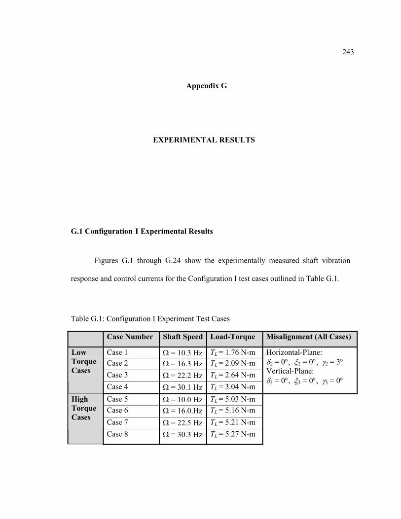
243

Appendix G

EXPERIMENTAL RESULTS

G.1 Configuration I Experimental Results

Figures G.1 through G.24 show the experimentally measured shaft vibration

response and control currents for the Configuration I test cases outlined in Table G.1.

Table G.1: Configuration I Experiment Test Cases


Case 1 Ω = 10.3 Hz TL = 1.76 N-mCase 2 Ω = 16.3 Hz TL = 2.09 N-mCase 3 Ω = 22.2 Hz TL = 2.64 N-m

LowTorqueCases

Case 4 Ω = 30.1 Hz TL = 3.04 N-m

Horizontal-Plane:δ2 = 0°, ξ2 = 0°, γ2 = 3°Vertical-Plane:δ3 = 0°, ξ3 = 0°, γ3 = 0°

Case 5 Ω = 10.0 Hz TL = 5.03 N-mCase 6 Ω = 16.0.Hz TL = 5.16 N-mCase 7 Ω = 22.5 Hz TL = 5.21 N-m

HighTorqueCases

Case 8 Ω = 30.3 Hz TL = 5.27 N-m

244

G.1.1 Configuration I Time-Domain Results

The figures in this sub-section give the time-domain shaft vibration

response and control currents for the Configuration I test cases.

0 50 100 150 200-225

0

225

0 50 100 150 200-225

0

225

0 50 100 150 200-225

0

225

0 50 100 150 200-225

0

225

0 50 100 150 200-225

0

225

0 50 100 150 200-225

0

225

time, sec

v-di

r di

sp.

AM

B3,

µm PID PID-MHAVC

v-di

r di

sp.

AM

B2,

µm

v-di

r di

sp.

AM

B1,

µm

Activate MHAVC w-di

r di

sp.

AM

B3,

µm

w-di

r di

sp.

AM

B2,

µm

w-d

ir d

isp.

AM

B1,

µm

Fig. G.1: Configuration I shaft vibration response, Case 1.

245

0 50 100 150 200-0.1

00.10.20.3

0 50 100 150 2000

0.2

0.4

0 50 100 150 200

-0.1

0

0.1

0 50 100 150 200-0.1

0

0.1

0.2

0 50 100 150 200

-0.4

-0.2

0

0 50 100 150 200

-0.2

0

0.2

v-di

r cu

rren

t.A

MB

3, A

mps

PIDPID-MHAVC

v-di

r cu

rren

t.A

MB

2, A

mps

v-di

r cu

rren

t.A

MB

1, A

mps

w-di

r cu

rren

t.A

MB

3, A

mps

w-di

r cu

rren

t.A

MB

2, A

mps

w-di

r cu

rren

t.A

MB

1, A

mps

time, sec

Activate MHAVC

Fig. G.2: Configuration I control current, Case 1.

0 50 100 150 200-225

0

225

0 50 100 150 200-225

0

225

0 50 100 150 200-225

0

225

0 50 100 150 200-225

0

225

0 50 100 150 200-225

0

225

0 50 100 150 200-225

0

225

v-di

r di

sp.

AM

B3,

µm PID PID-MHAVC

v-di

r di

sp.

AM

B2,

µm

v-di

r di

sp.

AM

B1,

µm

Activate MHAVC w-di

r di

sp.

AM

B3,

µm

w-di

r di

sp.

AM

B2,

µm

w-di

r di

sp.

AM

B1,

µm

time, sec


246

0 50 100 150 200

0

0.2

0.4

0 50 100 150 2000

0.2

0.4

0 50 100 150 200

-0.1

0

0.1

0 50 100 150 200

-0.1

0

0.1

0.2

0 50 100 150 200

-0.4

-0.3

-0.2

-0.1

0 50 100 150 200

-0.2

0

0.2

Activate MHAVCv-di

r cu

rren

t.A

MB

3, A

mps

v-di

r cu

rren

t.A

MB

2, A

mps

v-di

r cu

rren

t.A

MB

1, A

mps

w-di

r cu

rren

t.A

MB

3, A

mps

w-di

r cu

rren

t.A

MB

2, A

mps

w-di

r cu

rren

t.A

MB

1, A

mps

time, sec


0 50 100 150 200-225

0

225

0 50 100 150 200-225

0

225

0 50 100 150 200-225

0

225

0 50 100 150 200-225

0

225

0 50 100 150 200-225

0

225

0 50 100 150 200-225

0

225

v-di

r di

sp.

AM

B3,

µm PID PID-MHAVC

v-di

r di

sp.

AM

B2,

µm

v-di

r di

sp.

AM

B1,

µm

Activate MHAVC w-di

r di

sp.

AM

B3,

µm

w-d

ir d

isp.

AM

B2,

µm

w-d

ir d

isp.

AM

B1,

µm

time, sec


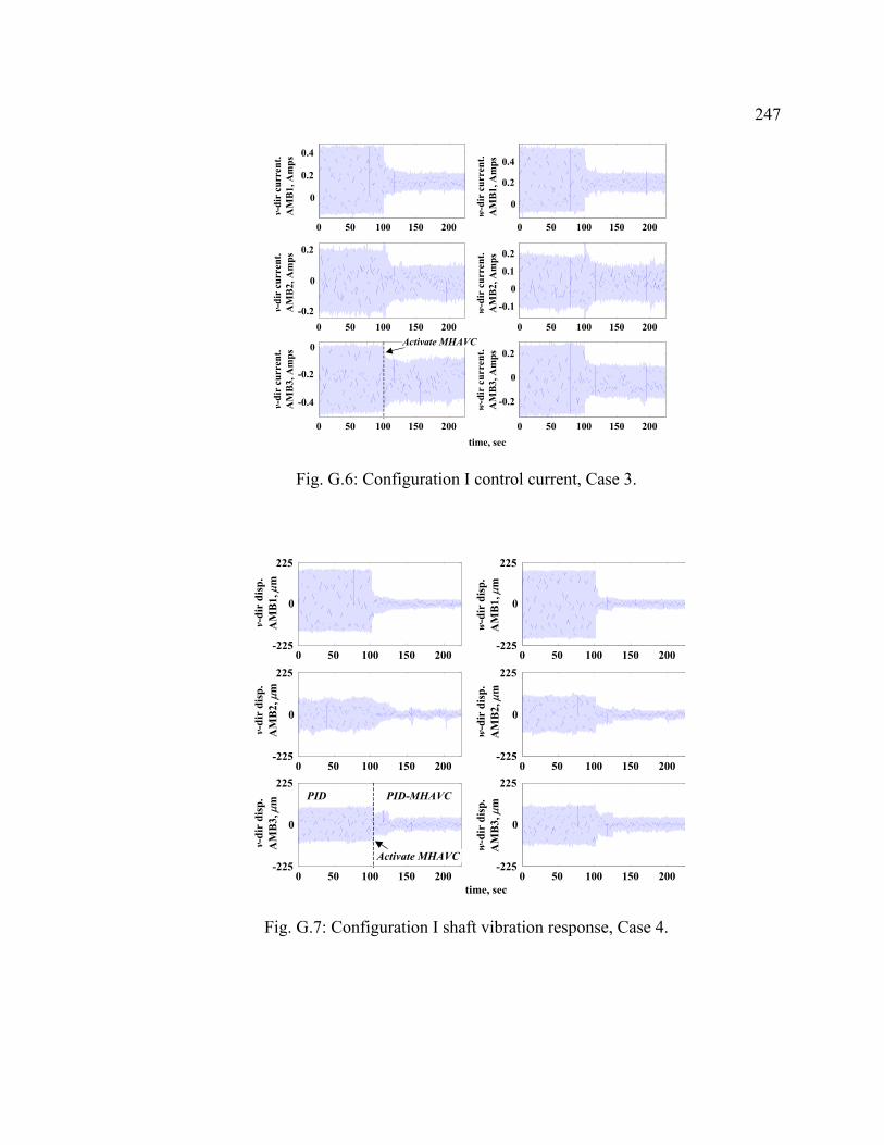
247

0 50 100 150 200

0

0.2

0.4

0 50 100 150 200

0

0.2

0.4

0 50 100 150 200-0.2

0

0.2

0 50 100 150 200

-0.1

0

0.1

0.2

0 50 100 150 200

-0.4

-0.2

0

0 50 100 150 200

-0.2

0

0.2Activate MHAVC

v-di

r cu

rren

t.A

MB

3, A

mps

v-di

r cu

rren

t.A

MB

2, A

mps

v-di

r cu

rren

t.A

MB

1, A

mps

w-di

r cu

rren

t.A

MB

3, A

mps

w-di

r cu

rren

t.A

MB

2, A

mps

w-di

r cu

rren

t.A

MB

1, A

mps

time, sec


0 50 100 150 200-225

0

225

0 50 100 150 200-225

0

225

0 50 100 150 200-225

0

225

0 50 100 150 200-225

0

225

0 50 100 150 200-225

0

225

0 50 100 150 200-225

0

225PID PID-MHAVC

Activate MHAVC

time, sec

v-di

r di

sp.

AM

B3,

µm

v-di

r di

sp.

AM

B2,

µm

v-di

r di

sp.

AM

B1,

µm

w-di

r di

sp.

AM

B3,

µm

w-di

r di

sp.

AM

B2,

µm

w-di

r di

sp.

AM

B1,

µm


248

0 50 100 150 200

-0.20

0.20.40.6

0 50 100 150 200-0.2

00.20.40.6

0 50 100 150 200

-0.2

0

0.2

0 50 100 150 200

-0.2

0

0.2

0.4

0 50 100 150 200-0.8-0.6-0.4-0.2

0

0 50 100 150 200

-0.4-0.2

00.20.4

ActivateMHAVC

time, sec

v-di

r cu

rren

t.A

MB

3, A

mps

v-di

r cu

rren

t.A

MB

2, A

mps

v-di

r cu

rren

t.A

MB

1, A

mps

w-di

r cu

rren

t.A

MB

3, A

mps

w-d

ir c

urre

nt.

AM

B2,

Am

psw-

dir

curr

ent.

AM

B1,

Am

psFig. G.8: Configuration I control current, Case 4.

0 50 100 150 200-225

0

225

0 50 100 150 200-225

0

225

0 50 100 150 200-225

0

225

0 50 100 150 200-225

0

225

0 50 100 150 200-225

0

225

0 50 100 150 200-225

0

225

v-di

r di

sp.

AM

B3,

µm PID PID-MHAVC

v-di

r di

sp.

AM

B2,

µm

v-di

r di

sp.

AM

B1,

µm

Activate MHAVC

w-d

ir d

isp.

AM

B3,

µm

w-d

ir d

isp.

AM

B2,

µm

w-d

ir d

isp.

AM

B1,

µm

time, sec


249

0 50 100 150 200-0.2

0

0.2

0.4

0 50 100 150 200

0

0.2

0.4

0.6

0 50 100 150 200-0.1

0

0.1

0.2

0 50 100 150 200

-0.1

0

0.1

0 50 100 150 200

-0.6

-0.4

-0.2

0 50 100 150 200

-0.2

0

0.2

Activate MHAVC

time, sec

v-di

r cu

rren

t.A

MB

3, A

mps

v-di

r cu

rren

t.A

MB

2, A

mps

v-di

r cu

rren

t.A

MB

1, A

mps

w-d

ir c

urre

nt.

AM

B3,

Am

psw-

dir

curr

ent.

AM

B2,

Am

psw-

dir

curr

ent.

AM

B1,

Am


0 50 100 150 200-225

0

225

0 50 100 150 200-225

0

225

0 50 100 150 200-225

0

225

0 50 100 150 200-225

0

225

0 50 100 150 200-225

0

225

0 50 100 150 200-225

0

225

v-di

r di

sp.

AM

B3,

µm

PID PID-MHAVC

v-di

r di

sp.

AM

B2,

µm

v-di

r di

sp.

AM

B1,

µm

Activate MHAVC w-di

r di

sp.

AM

B3,

µm

w-di

r di

sp.

AM

B2,

µm

w-di

r di

sp.

AM

B1,

µm

time, sec


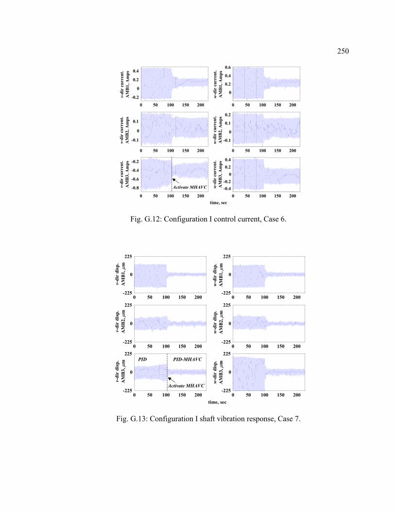
250

0 50 100 150 200

-0.2

0

0.2

0.4

0 50 100 150 200

0

0.2

0.4

0.6

0 50 100 150 200

-0.1

0

0.1

0 50 100 150 200

-0.1

0

0.1

0.2

0 50 100 150 200

-0.8

-0.6

-0.4

-0.2

0 50 100 150 200-0.4-0.2

00.20.4

Activate MHAVC

time, sec

v-di

r cu

rren

t.A

MB

3, A

mps

v-di

r cu

rren

t.A

MB

2, A

mps

v-di

r cu

rren

t.A

MB

1, A

mps

w-di

r cu

rren

t.A

MB

3, A

mps

w-di

r cu

rren

t.A

MB

2, A

mps

w-di

r cu

rren

t.A

MB

1, A

mps


0 50 100 150 200-225

0

225

0 50 100 150 200-225

0

225

0 50 100 150 200-225

0

225

0 50 100 150 200-225

0

225

0 50 100 150 200-225

0

225

0 50 100 150 200-225

0

225

v-di

r di

sp.

AM

B3,

µm PID PID-MHAVC

v-di

r di

sp.

AM

B2,

µm

v-di

r di

sp.

AM

B1,

µm

Activate MHAVC

w-di

r di

sp.

AM

B3,

µm

w-di

r di

sp.

AM

B2,

µm

w-di

r di

sp.

AM

B1,

µm

time, sec


251

0 50 100 150 200

0

0.2

0.4

0 50 100 150 200

0

0.2

0.4

0.6

0 50 100 150 200-0.2

0

0.2

0 50 100 150 200-0.2

0

0.2

0 50 100 150 200

-0.8

-0.6

-0.4

0 50 100 150 200-0.5

0

0.5

Activate MHAVC

time, sec

v-di

r cu

rren

t.A

MB

3, A

mps

v-di

r cu

rren

t.A

MB

2, A

mps

v-di

r cu

rren

t.A

MB

1, A

mps

w-d

ir c

urre

nt.

AM

B3,

Am

psw-

dir

curr

ent.

AM

B2,

Am

psw-

dir

curr

ent.

AM

B1,

Am


0 50 100 150 200-225

0

225

0 50 100 150 200-25

0

225

0 50 100 150 200-225

0

225

0 50 100 150 200-225

0

225

0 50 100 150 200-225

0

225

0 50 100 150 200-225

0

225

v-di

r di

sp.

AM

B3,

µm PID PID-MHAVC

v-di

r di

sp.

AM

B2,

µm

v-di

r di

sp.

AM

B1,

µm

Activate MHAVC

w-di

r di

sp.

AM

B3,

µm

w-di

r di

sp.

AM

B2,

µm

w-di

r di

sp.

AM

B1,

µm

time, sec


252

G.1.2 Configuration I Frequency-Domain Results

The figures in this sub-section give the spectrum of the steady-state shaft

vibration response for each of the Configuration I experimental test cases. Here, the

response spectrum at each operating condition is computed via an FFT analysis.

0 50 100 150 200

-0.20

0.20.40.6

0 50 100 150 200-0.2

00.20.4

0.6

0 50 100 150 200

-0.2

0

0.2

0 50 100 150 200

-0.2

0

0.2

0 50 100 150 200

-0.8

-0.6

-0.4

-0.2

0 50 100 150 200-0.4

-0.2

0

0.2

0.4ActivateMHAVC

time, sec

v-di

r cu

rren

t.A

MB

3, A

mps

v-di

r cu

rren

t.A

MB

2, A

mps

v-di

r cu

rren

t.A

MB

1, A

mps

w-d

ir c

urre

nt.

AM

B3,

Am

psw

-dir

cur

rent

.A

MB

2, A

mps

w-di

r cu

rren

t.A

MB

1, A

mps


253

0 20 40 60 80 100 120 1400

1020

304050

0 20 40 60 80 100 120 1400

1020

304050

0 20 40 60 80 100 120 1400

10

20

30

4050

0 20 40 60 80 100 120 1400

10

20

30

4050

0 20 40 60 80 100 120 1400

10

203040

50

0 20 40 60 80 100 120 1400

10

203040

50

Frequency, Hz

Shaf

t Vib

ratio

n A

mpl

itude

, µm

(PI

D)







Shaf

t Vib

ratio

n A

mpl

itude

, µm

(PI

D-M

HA

VC

)

Ω

2Ω

3Ω

4Ω

72.4 µm“peak”

Fig. G.17: Configuration I shaft vibration spectrum, Case 1.

0 20 40 60 80 100 120 1400

1020

3040

50

0 20 40 60 80 100 120 1400

1020

30

40

50

0 20 40 60 80 100 120 1400

102030

4050

0 20 40 60 80 100 120 1400

102030

4050

0 20 40 60 80 100 120 1400

10

20

30

4050

0 20 40 60 80 100 120 1400

10

2030

4050

Frequency, Hz

Shaf

t Vib

ratio

n A

mpl

itude

, µm

(PI

D)







Shaf

t Vib

ratio

n A

mpl

itude

, µm

(PI

D-M

HA

VC

)

2Ω

4Ω

83.9 µm“peak”

Ω

3Ω


254

0 20 40 60 80 100 120 1400

1020

3040

50

0 20 40 60 80 100 120 1400

1020

3040

50

0 20 40 60 80 100 120 1400

102030

4050

0 20 40 60 80 100 120 1400

102030

4050

0 20 40 60 80 100 120 1400

10

2030

40

50

0 20 40 60 80 100 120 1400

10

2030

40

50

Frequency, Hz

Shaf

t Vib

ratio

n A

mpl

itude

, µm

(PI

D)







Shaf

t Vib

ratio

n A

mpl

itude

, µm

(PI

D-M

HA

VC

)

Ω 2Ω

3Ω 4Ω

98.4 µm“peak”


0 20 40 60 80 100 120 1400

1020

3040

50

0 20 40 60 80 100 120 1400

1020

3040

50

0 20 40 60 80 100 120 1400

102030

4050

0 20 40 60 80 100 120 1400

102030

4050

0 20 40 60 80 100 120 1400

10

2030

4050

0 20 40 60 80 100 120 1400

10

2030

4050

Frequency, Hz

Shaf

t Vib

ratio

n A

mpl

itude

, µm

(PI

D)







Shaf

t Vib

ratio

n A

mpl

itude

, µm

(PI

D-M

HA

VC

)

Ω

2Ω3Ω 4Ω

142.2 µm“peak”

67.3 µm“peak”

56.8 µm“peak”


255

0 20 40 60 80 100 120 1400

1020

3040

50

0 20 40 60 80 100 120 1400

1020

3040

50

0 20 40 60 80 100 120 1400

102030

4050

0 20 40 60 80 100 120 1400

102030

4050

0 20 40 60 80 100 120 1400

10

2030

4050

0 20 40 60 80 100 120 1400

10

2030

4050

Frequency, Hz

Shaf

t Vib

ratio

n A

mpl

itude

, µm

(PI

D)







Shaf

t Vib

ratio

n A

mpl

itude

, µm

(PI

D-M

HA

VC

)

Ω

2Ω

3Ω

4Ω

110.6 µm“peak”


0 20 40 60 80 100 120 1400

1020304050

0 20 40 60 80 100 120 1400

1020304050

0 20 40 60 80 100 120 1400

1020304050

0 20 40 60 80 100 120 1400

1020304050

0 20 40 60 80 100 120 1400

1020304050

0 20 40 60 80 100 120 1400

1020304050

Frequency, Hz

Shaf

t Vib

ratio

n A

mpl

itude

, µm

(PI

D)







Shaf

t Vib

ratio

n A

mpl

itude

, µm

(PI

D-M

HA

VC

)

Ω2Ω

3Ω4Ω

128.2 µm“peak”

79.3 µm


256

0 20 40 60 80 100 120 1400

1020304050

0 20 40 60 80 100 120 1400

1020304050

0 20 40 60 80 100 120 1400

1020304050

0 20 40 60 80 100 120 1400

1020304050

0 20 40 60 80 100 120 1400

1020304050

0 20 40 60 80 100 120 1400

1020304050

Frequency, Hz

Shaf

t Vib

ratio

n A

mpl

itude

, µm

(PI

D)







Shaf

t Vib

ratio

n A

mpl

itude

, µm

(PI

D-M

HA

VC

)

Ω 2Ω

3Ω 4Ω

105.1 µm“peak”

113.8 µm“peak”


0 20 40 60 80 100 120 1400

1020304050

0 20 40 60 80 100 120 1400

1020304050

0 20 40 60 80 100 120 1400

1020304050

0 20 40 60 80 100 120 1400

1020304050

0 20 40 60 80 100 120 1400

1020304050

0 20 40 60 80 100 120 1400

1020304050

Frequency, Hz

Shaf

t Vib

ratio

n A

mpl

itude

, µm

(PI

D)







Shaf

t Vib

ratio

n A

mpl

itude

, µm

(PI

D-M

HA

VC

)

Ω2Ω

3Ω 4Ω

118.9 µm“peak”

68.7 µm“peak”


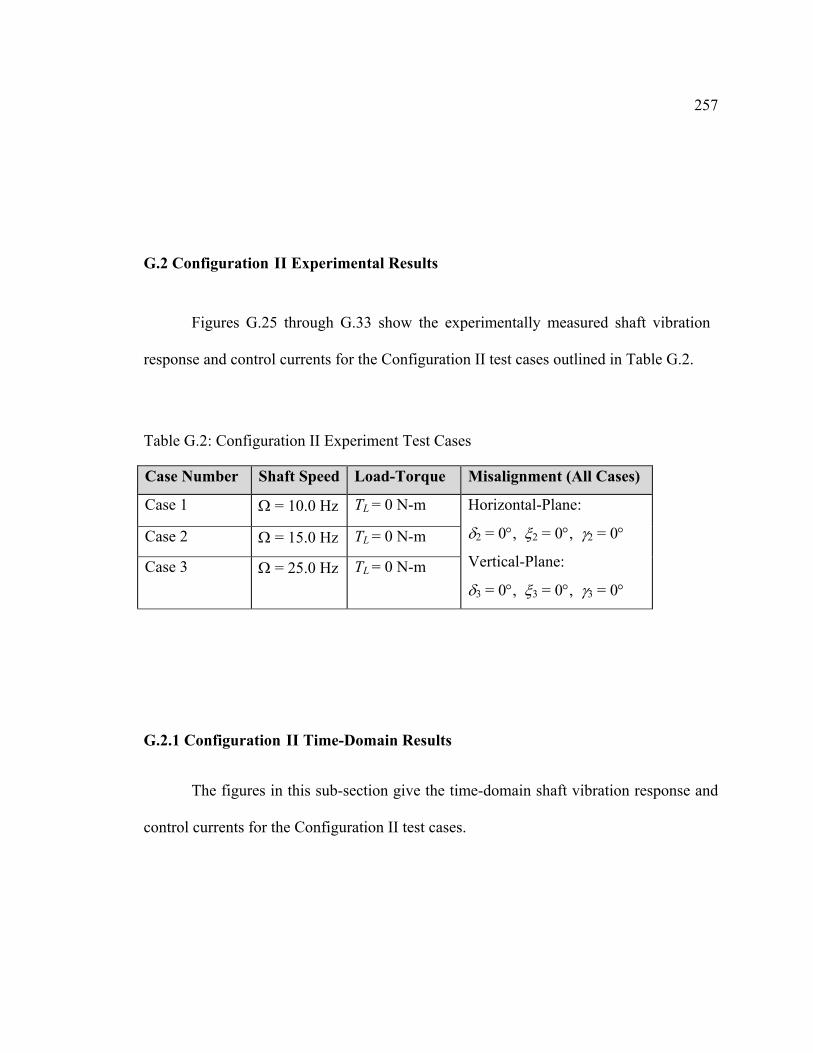
257

G.2 Configuration II Experimental Results

Figures G.25 through G.33 show the experimentally measured shaft vibration

response and control currents for the Configuration II test cases outlined in Table G.2.

G.2.1 Configuration II Time-Domain Results

The figures in this sub-section give the time-domain shaft vibration response and

control currents for the Configuration II test cases.

Table G.2: Configuration II Experiment Test Cases


Case 1 Ω = 10.0 Hz TL = 0 N-m

Case 2 Ω = 15.0 Hz TL = 0 N-m

Case 3 Ω = 25.0 Hz TL = 0 N-m

Horizontal-Plane:

δ2 = 0°, ξ2 = 0°, γ2 = 0°

Vertical-Plane:

δ3 = 0°, ξ3 = 0°, γ3 = 0°

258

0 50 100 150 200 250 0 50 100 150 200 250

0 50 100 150 200 250 0 50 100 150 200 250

0 50 100 150 200 250 0 50 100 150 200 250

0 50 100 150 200 250 0 50 100 150 200 250

-225

0

225

-225

0

225

-225

0

225

-225

0

225

-225

0

225

-225

0

225

-225

0

225

-225

0

225

w-di

r di

sp.

AM

B1,

µm

w-di

r di

sp.

AM

B2,

µm

w-di

r di

sp.

AM

B3,

µm

w-di

r di

sp.

AM

B4,

µm

v-di

r di

sp.

AM

B1,

µm

v-di

r di

sp.

AM

B2,

µm

v-di

r di

sp.

AM

B3,

µm

v-di

r di

sp.

AM

B4,

µm PID PID-SAVC

Activate SAVC

time, sec

Fig. G.25: Configuration II shaft vibration response, Case 1.

0 50 100 150 200 250

0.2

0.4

0 50 100 150 200 250

-0.10

0.10.2

0 50 100 150 200 250

0

0.1

0.2

0 50 100 150 200 2500.1

0.2

0.3

0 50 100 150 200 2500

0.10.20.3

0 50 100 150 200 250

00.10.20.3

0 50 100 150 200 2500

0.10.20.3

0 50 100 150 200 250

00.10.20.3

v-di

r cu

rren

tA

MB

1, A

mps

v-di

r cu

rren

tA

MB

2, A

mps

v-di

r cu

rren

tA

MB

3, A

mps

v-di

r cu

rren

tA

MB

4, A

mps

w-di

r cu

rren

tA

MB

1, A

mps

w-di

r cu

rren

tA

MB

2, A

mps

w-di

r cu

rren

tA

MB

3, A

mps

w-di

r cu

rren

tA

MB

4, A

mps

time, secActivate SAVC

Fig. G.26: Configuration II control current, Case 1.

259

0 50 100 150 200 250 0 50 100 150 200 250

0 50 100 150 200 250 0 50 100 150 200 250

0 50 100 150 200 250 0 50 100 150 200 250

0 50 100 150 200 250 0 50 100 150 200 250

-225

0

225

-225

0

225

-225

0

225

-225

0

225

-225

0

225

-225

0

225

-225

0

225

-225

0

225

w-d

ir d

isp.

AM

B1,

µm

w-d

ir d

isp.

AM

B2,

µm

w-d

ir d

isp.

AM

B3,

µm

w-d

ir d

isp.

AM

B4,

µm

v-di

r di

sp.

AM

B1,

µm

v-di

r di

sp.

AM

B2,

µm

v-di

r di

sp.

AM

B3,

µm

v-di

r di

sp.

AM

B4,

µm

time, sec


0 50 100 150 200 250

0.2

0.4

0 50 100 150 200 250

-0.10

0.10.2

0 50 100 150 200 250

0

0.1

0.2

0 50 100 150 200 2500.1

0.2

0.3

0 50 100 150 200 2500

0.10.20.3

0 50 100 150 200 250

00.10.20.3

0 50 100 150 200 2500

0.10.20.3

0 50 100 150 200 250

00.10.20.3

v-di

r cu

rren

tA

MB

1, A

mps

v-di

r cu

rren

tA

MB

2, A

mps

v-di

r cu

rren

tA

MB

3, A

mps

v-di

r cu

rren

tA

MB

4, A

mps

w-d

ir c

urre

ntA

MB

1, A

mps

w-di

r cu

rren

tA

MB

2, A

mps

w-d

ir c

urre

ntA

MB

3, A

mps

w-di

r cu

rren

tA

MB

4, A

mps



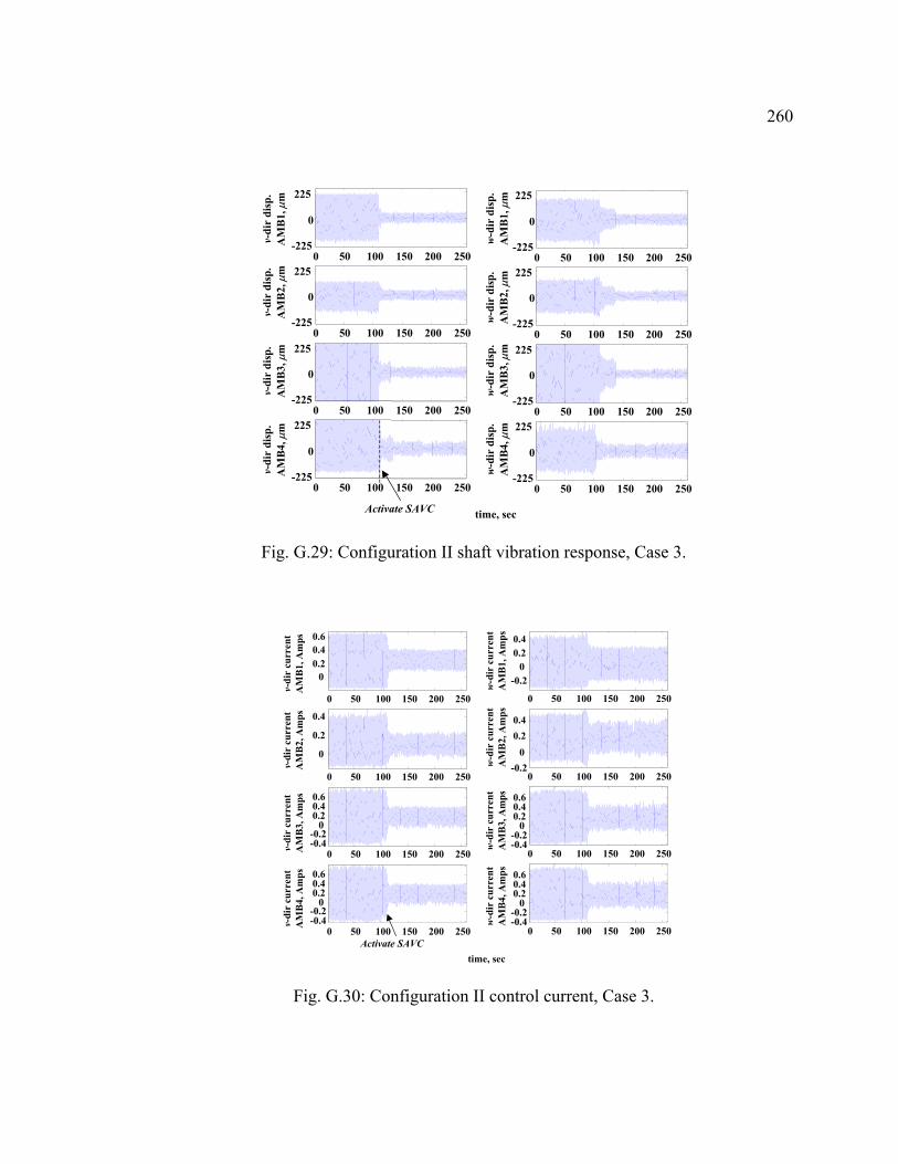
260

0 50 100 150 200 250-225

0

225

0 50 100 150 200 250-225

0

225

0 50 100 150 200 250-225

0

225

0 50 100 150 200 250-225

0

225

0 50 100 150 200 250-225

0

225

0 50 100 150 200 250-225

0

225

0 50 100 150 200 250-225

0

225

0 50 100 150 200 250-225

0

225

w-di

r di

sp.

AM

B1,

µm

w-di

r di

sp.

AM

B2,

µm

w-di

r di

sp.

AM

B3,

µm

w-di

r di

sp.

AM

B4,

µm

v-di

r di

sp.

AM

B1,

µm

v-di

r di

sp.

AM

B2,

µm

v-di

r di

sp.

AM

B3,

µm

v-di

r di

sp.

AM

B4,

µm



0 50 100 150 200 250 0 50 100 150 200 250

0 50 100 150 200 250 0 50 100 150 200 250

0 50 100 150 200 250 0 50 100 150 200 250

0 50 100 150 200 250

-0.2

0.6

0

0

00.20.40.6

0

0.2

0.4

-0.4

0.20.4

-0.4-0.2

0.20.40.6

0 50 100 150 200 250

-0.2

0.2

0.6

-0.2

0.2

0.6

-0.20

0.20.4

-0.20

0.20.4

-0.4

0

0.4

-0.4

0

0.4

v-di

r cu

rren

tA

MB

1, A

mps

v-di

r cu

rren

tA

MB

2, A

mps

v-di

r cu

rren

tA

MB

3, A

mps

v-di

r cu

rren

tA

MB

4, A

mps

w-di

r cu

rren

tA

MB

1, A

mps

w-di

r cu

rren

tA

MB

2, A

mps

w-d

ir c

urre

ntA

MB

3, A

mps

w-di

r cu

rren

tA

MB

4, A

mps



261

G.2.2 Configuration II Frequency-Domain Results

The figures in this sub-section give the spectrum of the steady-state shaft

vibration response for each of the Configuration II experimental test cases. Here, the

response spectrum at each operating condition is computed via an FFT analysis.

0 20 40 60 80 100 120 140

0 20 40 60 80 100 120 140

0 20 40 60 80 100 120 140

0 20 40 60 80 100 120 140

020406080

020406080

020406080

020406080

0 20 40 60 80 100 120 140

0 20 40 60 80 100 120 140

0 20 40 60 80 100 120 140

0 20 40 60 80 100 120 140

020406080

020406080

020406080

020406080

Frequency, Hz

Shaf

t Vib

ratio

n A

mpl

itude

, µm

(PI

D)

Shaf

t Vib

ratio

n A

mpl

itude

, µm

(PI

D-M

HA

VC

)









Ω

Fig. G.31: Configuration II shaft vibration spectrum, Case 1.

262

0 20 40 60 80 100 120 140 0 20 40 60 80 100 120 140

0 20 40 60 80 100 120 140 0 20 40 60 80 100 120 140

0 20 40 60 80 100 120 140 0 20 40 60 80 100 120 140

0 20 40 60 80 100 120 140

020406080

020406080

020406080

020406080

0 20 40 60 80 100 120 140

020406080

020406080

020406080

020406080

Frequency, Hz

Shaf

t Vib

ratio

n A

mpl

itude

, µm

(PI

D)

Shaf

t Vib

ratio

n A

mpl

itude

, µm

(PI

D-M

HA

VC

)









Ω


263

Note, in Case 3 of Configuration II, the PID controlled shaft imbalance vibration

response amplitudes exceeds the AMB backup-bearing clearances resulting periodic

shaft/backup-bearing impacts, see Figure G.29. This non-linear impact phenomena

results in a multi-harmonic response which is observed in Figure G.33 for the system

under PID control. However, once the Synchronous Adaptive Vibration Control (SAVC)

is activated, the synchronous portion of the response is suppressed and the contact is

prevented.

0 20 40 60 80 100 120 140

0 20 40 60 80 100 120 140

0 20 40 60 80 100 120 140

0 20 40 60 80 100 120 140

020406080

020406080

020406080

020406080

0 20 40 60 80 100 120 140

0 20 40 60 80 100 120 140

0 20 40 60 80 100 120 140

0 20 40 60 80 100 120 140

020406080

020406080

020406080

020406080









Frequency, Hz

Shaf

t Vib

ratio

n A

mpl

itude

, µm

(PI

D)

Shaf

t Vib

ratio

n A

mpl

itude

, µm

(PI

D-M

HA

VC

)Ω


VITA

Hans A. DeSmidt was born November 27, 1973 in Richmond Virginia, USA. He

graduated May 1992 from Hermitage High School in Henrico County, VA, where he

participated in the Virginia Junior Academy of Science and was a member of the

National Honor Society. In 1996, he graduated Summa Cum Laude with a B.S. degree in

Engineering Science and Mechanics from the Virginia Polytechnic Institute and State

University (Virginia Tech) in Blacksburg, VA. While attending Virginia Tech, he was a

member of Tau Beta Pi and Phi Eta Sigma engineering honor societies. Additionally, in

1994 and 1995, he was awarded to participate in the National Science Foundation

Summer Undergraduate Research Program (NSF-SURP), where he published two

undergraduate research papers on the topic composite materials. In 1996, he began is

graduate studies in the Mechanical Engineering Department at The Pennsylvania State

University, in University Park, PA, where he was both a NASA Graduate Student

Research Program (GSRP) fellow and a Weiss Graduate Research Fellow. His research

and course work was in the areas of Structural Dynamics, Vibrations, Rotordynamics,

Active Control Theory, and Magnetic Bearing technology. While conducting his Ph.D.

thesis investigation, he published seven conference papers and three academic journal

papers on topics concerning various aspects of his research. Finally, he is both a member

of the American Society of Mechanical Engineers (ASME) and the American Helicopter

Society (AHS).

the pennsylvania state university the graduate school college of

Documents