the performance of hedge fund strategies in emerging...
TRANSCRIPT

The Performance of Hedge Fund Strategies in Emerging Markets
Authors: Oliwer Berglund & Henrik Fahlström Jönköping May 2017
i
Bachelor Thesis in Economics Title: The performance of hedge fund strategies in emerging markets Authors: Oliwer Berglund and Henrik Fahlström Tutor: Johan P. Larsson Amedeus Malisa Date: 2017-05-22 Key terms: Hedge fund, Hedge Fund Performance, Alpha, Hedge Fund Strategies, Emerging Markets Abstract In the past decades, emerging market hedge funds have been subject to significant capital inflow
and today they constitute a $200 billion market. Previous research suggests that future investment
opportunities exist in these regions. The objective of this study is to examine if emerging market
hedge funds produce higher risk-adjusted returns than global hedge funds, focusing on how
different hedge fund investment strategies perform. The research is based on the single factor
Capital Asset Pricing Model (CAPM) to determine the strategies performance (alpha) net of fees.
The study ranges from January 2002 to December 2016 and scrutinizes the strategies performance
in seven different sub-periods. The research provides evidence that the magnitude of performance
for hedge funds differ not only regarding the location of which fund managers choose to allocate
the assets, but also on what kind of strategy they practice to generate return. On a risk-adjusted
premise, the study finds that not all strategies in emerging markets manage to perform better than
the global hedge fund market consistently over a longer period. These findings stress the
importance of considering fund strategies rather than location, when comparing financial
instruments. The conclusions provide helpful knowledge to both future research and financial
authorities.

ii
Table of Contents 1 Introduction .............................................................................. 1 1.1 Background .................................................................................................................... 1 1.2 Problem statement ........................................................................................................ 2 1.3 Purpose .......................................................................................................................... 2
2 Hedge funds ............................................................................. 3 2.1 Hedging .......................................................................................................................... 3 2.2 Emerging markets ......................................................................................................... 3 2.3 What are hedge funds ................................................................................................... 3 2.4 Hedge funds vs. mutual funds...................................................................................... 4 2.5 Hedge fund strategies .................................................................................................... 4 2.6 Classification of hedge fund strategies ........................................................................ 5 2.6.1 Arbitrage ........................................................................................................................ 5 2.6.2 Managed futures ............................................................................................................ 5 2.6.3 Event driven .................................................................................................................. 6 2.6.4 Long and short positions .............................................................................................. 6 2.6.5 Fixed income ................................................................................................................. 6 2.7 Related literature ............................................................................................................ 6
3 Theoretical framework .............................................................. 9 3.1 Efficient market hypothesis .......................................................................................... 9 3.2 Modern Portfolio Theory ............................................................................................. 9 3.3 Capital asset pricing model and the efficient market portfolio................................ 10
4 Empirical measurements ......................................................... 11 4.1 Beta ............................................................................................................................... 11 4.2 Jensen’s alpha ............................................................................................................... 11 4.3 Skewness and kurtosis ................................................................................................. 12
5 Method and data ...................................................................... 14 5.1 Method ......................................................................................................................... 14 5.2 Sample selection and data collection ......................................................................... 14 5.3 Variables ....................................................................................................................... 15 5.4 Performance measurement ......................................................................................... 15 5.5 Data analysis ................................................................................................................ 15 5.6 Quality of method ....................................................................................................... 16 5.7 Potential biases ............................................................................................................ 16
6 Empirical results ...................................................................... 18 6.1 Descriptive statistics .................................................................................................... 18 6.2 Correlation ................................................................................................................... 20 6.3 Performance measurement results ............................................................................. 21 6.4 Performance in different market environments ....................................................... 26
7 Conclusion .............................................................................. 29 7.1 Future research ............................................................................................................ 30
References ............................................................................................ 31
Appendices .......................................................................................... 36

iii
Figures Figure 1: The Security Market Line, SML ............................................................................ 12 Figure 2: Skewness and kurtosis distributions ..................................................................... 13 Figure 3: Combinations of risk and return for hedge funds .............................................. 20 Figure 4: The change in estimated alpha ............................................................................. 25 Figure 5: The change in estimated beta................................................................................ 25 Figure 6: Strategy returns in different environments .......................................................... 26
Tables
Table 1: Comparison of Hedge funds and mutual funds ..................................................... 4 Table 2: Descriptive statistics: monthly excess returns....................................................... 18 Table 3: Descriptive statistic: monthly returns .................................................................... 18 Table 4: Correlation table ...................................................................................................... 21 Table 5: Regression result of the CAPM ............................................................................. 23
Equations Equation 1: Capital Asset Pricing Model, CAPM ............................................................... 10 Equation 2: Estimation of Beta ............................................................................................ 11 Equation 3: Estimation of Alpha ......................................................................................... 11

1
1 Introduction
1.1 Background
On several occasions during the past decades, the world has experienced economic distress,
such as the Asia Crisis, the IT-bubble and the recent Financial crisis (Ackermann, Richard,
& Ravenscraft, 1999; Amenc, Martellini, & Vaissié, 2002; Capocci & Hübner, 2004; Fung &
Hsieh, 2001). These crises have motivated investors to seek alternative investments options,
as a result, hedge funds have increased significantly in popularity and large amounts of wealth
are placed in this industry (Dichev & Yu, 2011; Liang, 1999). In contrast to other more
classical investments like stocks and bonds, the purpose of hedge funds is to generate
absolute returns, which means generating positive returns regardless of the market
movement (Ackermann et al., 1999; Agarwal & Naik, 2000). The opportunity to gain positive
returns in both growth and decreasing market environments are partly the reason for the
increased interest in hedge funds. Further, hedge funds are complex to define but are
characterized by their flexible strategies, lack of investment restrictions, limited licensing
requirements, strong managerial incentives and unrestricted allocation rules (Agarwal &
Naik, 2000; Brown, Goetzmann, & Ibbotson, 1999; Fung & Hsieh, 2004).
Despite indications of high risk and uncertainty, emerging markets are considered among the
most attractive investment regions in terms of growth opportunities (Amenc et al., 2002). A
substantial shift in asset allocation has taken place during the last decades, where the
aggregate market size of emerging markets has increased nearly 40 times, from $85 billion in
1990 to $3.8 trillion in 20141 (Lazard Asset Management, 2014). The growth opportunities
in emerging market regions have attracted the hedge fund industry as well. Even though
hedge funds have historically performed poorly in emerging markets, there is an upward
trend showing the opposite (Naik, Ramadorai, & Strömqvist, 2007; Strömqvist, 2008). At the
end of year 2016, $3.22 trillion worth of assets were held in hedge funds all over the world.
Out of these, $200 billion were allocated in the region of emerging markets2 (Datastream,
2017; Preqin, 2017).
1 Data is collected from MSCI. The MSCI Emerging Markets Index captures large and mid-cap representation across 23 Emerging Markets (EM) countries*. With 829 constituents, the index covers approximately 85% of the free float-adjusted market capitalization in each country. 2 In accordance with Eurekahedge (2017) we define “emerging markets” in this paper as developing Europe (Central and Eastern), Latin America, Russia, Asia (except Japan, Australia and New Zealand), Africa, Middle East and the Caribbean.

2
1.2 Problem statement
With barely any restrictions, hedge fund managers are handling large amounts of wealth using
complex investment strategies to chase absolute returns in uncertain markets (Ackermann et
al., 1999; Amenc et al., 2002; Naik et al., 2007). As the emerging markets are volatile, hedge
funds and emerging markets seem like a perfect fit and the combination of the two should,
in theory, be able to generate attractive returns (Eling & Faust, 2010; Strömqvist, 2007). The
problem is that there is yet little information about how they really perform.
Research within the field of hedge funds has increased together with its popularity. However,
the existing studies mainly conduct comparisons between hedge funds and passive
benchmarks (Ackermann et al.,1999; Agarwal & Naik, 2004; Amin & Kat, 2003; Liang,
1999), or study differences among hedge funds and mutual funds’ risk-adjusted performance
(Ackermann et al., 1999; Brown et al., 1999; Capocci and Hübner; 2004; Eling & Faust, 2010;
Liang 1999). Although hedge funds have received increased academic attention, research
regarding hedge funds’ behavior in emerging markets is limited. Existing studies in this field
often include and consider emerging markets as a strategy (Capocci & Hübner, 2004; Eling
& Faust, 2010). In turn, there are few studies on how different hedge fund strategies perform
in the region of emerging markets. Hence, there is an evident knowledge gap. Additionally,
due to the large amounts of assets that hedge fund managers are handling in these regions,
the performance is interesting to analyze.
1.3 Purpose
Because of the increased capital inflow in both hedge funds and the emerging market regions,
together with the existing knowledge gap, the purpose of this study is to examine how
different hedge fund investment strategies perform in emerging markets. The study will
attempt to answer the two following research questions:
1. Do emerging market hedge funds produce higher risk-adjusted returns than global hedge funds?
2. Is there a significant difference in performance depending on what strategy the hedge fund managers practice?

3
2 Hedge funds
2.1 Hedging
The word “hedging” describes a way to reduce risk exposure in an asset by adverse price
movements in a security. This is accomplished by the hedge taking a counter-position of the
related security (Connor & Woo, 2004). There is a trade-off between risk and reward, and
some reward must be paid to reduce the potential risk (Mossin, 1966). A hedge that manages
to eliminate all the systematic risk in a portfolio is considered a perfect hedge3. That is, the
hedge is completely inversely correlated with the exposed security (Capocci, 2013).
2.2 Emerging markets
Emerging market definitions usually vary, but can broadly be described as countries that
experience rapid growth and progressing into developed economies (Basu & Huang-Jones,
2015). The characteristics of emerging markets does come with a potential higher risk than
the developed markets and thereby also a chance of higher returns. Political instability, high
volatility, liquidity risk, exchange risks and poor corporate governance systems are some of
the factors that make emerging markers not as efficient as developed economies (Bekaert &
Harvey, 2002). Despite the uncertainties, emerging markets attract investors that seek high
returns and wants to benefit from diversification (Basu & Huang-Jones, 2015; Ratner & Leal,
2005).
2.3 What are hedge funds
Hedge funds are pooled investments that are managed actively as private partnerships. The
funds are directed towards a small group of investors; thus, the fund manager can be
described as the general partner and the fund’s investors as limited partners (Connor & Woo,
2004; Eling & Faust, 2010). As previously mentioned, one main objective of hedge funds is
to generate absolute return regardless of the market condition. Therefore, a low correlation
with the market is important regardless of what strategy the fund uses (Fung & Hsieh, 1997;
Liang, 1999). The fund management is intensely skill-based, as most hedge funds focus on
identifying speculations which can result in out-performing the market (Edwards &
Caglayan, 2001). Further, hedge funds are strongly driven by the fund managers’ incentives
and the managers are in general rewarded based on two fees: a performance based fee and a
3 Enough diversification eliminates unsystematic risk, more about the relationship in appendix 2.

4
management fee (Agarwal & Naik, 2000; Liang, 1999). In addition, the fund managers usually
invest a great amount of their own capital into the funds, which increases the performance
incentive substantially (Liang, 1999; Connor & Woo, 2004).
2.4 Hedge funds vs. mutual funds
Table 1 below presents the main features, and thereby the differences, of hedge funds and
mutual funds. Mutual funds are diversified as well as easy to buy and sell for the public;
almost any investor can access these funds and invest in publicly traded assets. In
comparison, hedge funds are private investment companies that have sophisticated investors
with a great net worth (Ackermann et al., 1999). Unlike mutual funds, hedge funds have lock-
up periods, which limit the ability to withdraw an investment. Although, the lock-up periods
also enable greater risk-taking for hedge funds as the fund manager knows when money can,
and will be, removed from the fund (Liang, 1999). Mutual fund managers are compelled to
report their performance, but there are no equivalent requirements for hedge fund managers.
Consequently, there is less accurate data for hedge funds as poor performing hedge funds
are often not reported (Strömqvist, 2009). Conclusively, there is also a difference regarding
the incentives of the two fund types. As stated above, the fee structures in hedge funds are
performance based, often with a bonus incentive. In contrast, the fee structures for mutual
funds are generally based on the fund size (Ackermann et al., 1999; Agarwal & Naik, 2000;
Liang, 1999).
Table 1: Comparison of Hedge funds and mutual funds Hedge fund Mutual fund Placement rules Free Limited Return target Absolute Relative Owners Few Thousands Investor type Pension funds, endowment
funds, high net worth individuals
Retail investors
Transparency Information for investors only Annual reports are published Fees Fixed and performance based Fixed
Note: Table 1illustrate how hedge funds and mutual funds differ in placement rules, returns target, owner style, investor types, information transparency and fee structure.
2.5 Hedge fund strategies
The investment strategy of a hedge fund determines how the fund is managed; hence, it
indicates how the manger will use investment techniques to generate the desired returns. The

5
strategies’ approach is crucial for the funds development and consequently, it is important
for the investors (Connor & Woo, 2004).
There are different opinions regarding how to categorize hedge fund strategies. In order to
display this debated categorization, three alternative approaches will be presented here. The
first categorization divides strategies by “location” and “style”. These two parameters
correspond to what position the investment takes; long or short, and what asset classes the
funds invest in; e.g. currencies, commodities etc. (Fung & Hsieh, 1997). The second
alternative categorizes strategies as “return enhancers” or “risk reducers”. Return enhancing
strategies target high returns with a generally higher portfolio risk. Risk reducing strategies
on the other hand, seek positive excess returns with a relatively lower risk in the portfolio
(Amenc et al., 2002). The third approach divides funds into market neutral or directional
funds. The neutral funds are characterized by low correlation with the market while
directional funds have higher correlation with the market since they speculate in market
fluctuations (Connor & Woo, 2004).
2.6 Classification of hedge fund strategies
Much like the situation regarding categorization of hedge fund strategies, there are several
different definitions of hedge fund strategies. Eurekahedge is one of the world’s largest
independent data providers of hedge fund information, and the five hedge fund strategies
presented below are in accordance with Eurekahedge’s classifications (2017).
2.6.1 Arbitrage
Arbitrage strategies are risk reducers. By purchasing and immediately reselling assets,
arbitrage strategies can take advantage of price inefficiencies in a variety of different or similar
market situations. Arbitrage strategies often have relatively low risk. These sorts of
transactions are almost independent of fluctuations in the market, which should make them
an efficient investment when there is a negative growth in the market (Eurekahedge, 2017).
2.6.2 Managed futures
Managed futures are investments in future contracts, completed through professional fund
managers both directly and through a Commodity Trading Advisor4, CTA. In general, CTAs
4 In the US, Commodity Trading Advisors, CTAs, need a license from the Commodity Futures Trading Commission.

6
use proprietary trading, which means that the investor invests primarily for his own sake
rather than for his clients. This is often done with help of complex computer programs where
they take long or short positions in future contracts including metals, grains, equity indexes,
commodities and foreign currencies. Managed futures decrease the risk of portfolios by
diversifying in different asset classes and investments types. Portfolios that use futures reduce
their risk due to the negative correlation among the securities in the portfolio (Eurekahedge,
2017).
2.6.3 Event driven
Event driven strategies are greatly speculative and depend heavily on the manager’s
information. They rely on information of events that will affect the market for a short period
of time: restrictions in corporations, stock buybacks, bond upgrades. They are not limited to
any specific investments style or class of assets (Eurekahedge, 2017).
2.6.4 Long and short positions
Long/short strategies are one of the most frequently used strategies. To hedge market risk,
investors take long- as well as short positions in the market. Doing so, managers can
speculate in price falls. By taking long and short positions, market risk is reduced through
risk in the individual stock (Eurekahedge, 2017).
2.6.5 Fixed income
The Fixed income strategy is a type of investment that relies on relatively predictable returns
at regular intervals. Fixed income strategies depend on mathematical programs that can
detect mispricing and manage positions. The focus is on interest rate swaps5 and mortgage-
backed securities (Eurekahedge, 2017).
2.7 Related literature
As stated above, the amount of literature on hedge fund strategies in emerging markets is
limited. There is however, research considering hedge funds in emerging markets and
strategies separately. The limited literature could be partly due to the narrow access to
individual funds data (Capocci & Hübner, 2004; Strömqvist, 2007).
5 The exchange of one set of cash flows for another at a given time

7
Fung and Hsieh (2011) and Eling and Faust (2010) studied long/short strategies and the
value-added they generate. In Fung and Hsieh (2011) sample of 3000 hedge funds using the
strategy, less than 20% of the funds produce positive alphas, which means they perform
better than the market. Furthermore, they found indications that alpha declines over time,
something that Fung, Hsieh and Ramadorai (2008) agree upon. In contrast, Strömqvist
(2007) argue that there is an upward trend for alphas and that they might be found in
emerging markets in the future. Eling and Faust (2010) also find evidence supporting positive
alphas in emerging markets. Furthermore, Eling and Faust (2010) find that hedge funds are
more efficient than mutual funds in allocating their assets, mainly due to the lack of
restrictions.
Ackermann et al. (1999), Brown et al. (1999), Capocci and Hübner (2004) and Liang (1999)
study differences among hedge funds and mutual funds’ risk-adjusted performance and their
persistence to generate return. Their findings are the same, and conclude that hedge funds
beat mutual funds on a regular basis, mostly due to the combination of incentive
arrangements and the investment flexibilities that hedge funds allow for (Ackermann et
al.,1999; Capocci & Hübner, 2004; Eling & Faust, 2010; Liang, 1999). In addition, hedge
funds have a higher volatility than mutual funds and the incentive fees can explain hedge
funds’ performance, but not the total risk in the portfolio (Ackermann et al.,1999). Brown et
al. (1999) find that the positive risk-adjusted return of offshore hedge funds6 are outcomes
of investment style rather than skills of fund managers. These findings are vital for the hedge
funds industry, since hedge funds tend to have higher attrition rate compared to mutual
funds (Agarwal & Naik, 2000; Brown, et al., 1999; Liang, 2000).
In existing research hedge funds often perform better than mutual funds, but not always the
compared benchmark (Ackermann et al., 1999; Brown et al. 1999; Capocci & Hübner, 2004;
Eling & Faust, 2010; Liang, 1999). Studies that examine hedge funds persistence performance
with passive index benchmarks, such as gold and the S&P 500 show mixed results (Agarwal
& Naik, 2004; Brown et al., 1999; Liang, 1999). Findings by Brown et al. (1999) and Liang
(1999) imply that hedge funds perform better than traditional benchmarks, while the results
by Agarwal and Naik (2004) vary significantly more.
6 Funds that are organized under foreign regulations. Outside the U.S. in the case of Brown et al. (1999)

8
Amin and Kat (2001) suggest that a greater risk-return profile cannot be offered by investing
in hedge funds alone due to inefficiency. Instead, hedge funds become efficient in
combination with passive benchmarks. This conclusion is in line with other studies, where
hedge funds appear to increase the return of a portfolio by having a weak correlation to other
securities in the market (Agarwal & Naik, 2000; Fung & Hsieh, 1997; Liang, 1999). Fung and
Hsieh (1997) find evidence that the risk-return profile improves in a portfolio when adding
hedge funds, mainly because of the low correlation with the market. Further, Amenc and
Martellini (2002) demonstrate that hedge funds that are included in a portfolio should result
in a decrease of risk without any change in return. Contrary, Strömqvist (2007) finds that
hedge fund performance has been weak historically, and suggests that hedge funds do not
provide any diversification benefit when combining it in a portfolio with other assets.
(Amenc & Martellini, 2002)

9
3 Theoretical framework
3.1 Efficient market hypothesis
The efficient market hypothesis has since its origin been the leading theory explaining how
price adjustments occur in markets. Financial markets are efficient and investors use
information provided by companies, often in the form of quarterly- and annual reports, but
also daily news and other analysis provided by different investors. Further, financial markets
are also competitive and quick to respond to information. Therefore, in a situation with
perfect information available, the market price would always represent the true price of a
security (Fama , 1970).
The efficient market hypothesis also implies that the market does not have any memory.
Hence, as new information becomes available, the security’s value can move up or down
towards its fundamental value. A stock that reacts on daily information does not have a
correlation with yesterday’s price level, which indicates a random walk7 and thereby a lack of
memory in the market (Clarke, Jandik, & Mandelker, 2001). There are however, certain
conditions that need to be fulfilled for the efficient market hypothesis to be valid8. Further,
the theory assumes that arbitrary gains are random and that the efficient market would be
impossible to out-perform without purchasing riskier assets (Fama & French, 2012).
3.2 Modern Portfolio Theory
Harry Markowitz was awarded with the Nobel Prize in Economics in 1990 for his theory
called The Modern Portfolio Theory (1952) that has become one of the most central
economic theories in the field of finance and investment (Elton & Gruber, 1997).
Markowitz’s theory assumes that investors are risk-averse and that they can build their
portfolio to maximize expected return at any given level of risk in the market. Furthermore,
the theory explains that it is inadequate to focus on the expected return and risk of one
specific security. Investors should rather invest in more than one security to reap the benefits
from diversification and reduce risk in the portfolio (Elton & Gruber, 1997; Markowitz,
1952).
7 Price changes have the same distribution and are independent of each other. 8 There cannot be any costs, such as brokerage fees, when you buy and sell securities. There cannot be any information asymmetries between the different operators on the market and there must be perfect information.
10
3.3 Capital asset pricing model and the efficient market portfolio
The Capital asset pricing model (CAPM) was founded and developed by William Sharpe
(1964) and is based on Harry Markowitz portfolio selection theory (1952). Still today, the
CAPM is used for various purposes such as evaluation of performance among managed
portfolios and to calculate the cost of capital (Fama & French, 2004).
The CAPM is a single factor model that describes the relationship between an assets
systematic risk and its expected return (Lintner, 1965; Perold, 2004). Within the scope of the
model, a market proxy9 is an estimation of the true market portfolio where the true market
portfolio is explained as a measurement for comparing different funds to the overall market
or industry (Roll, 1977). The return of the market and such a portfolio is almost impossible
to accomplish. Additionally, Richard Roll (1977) showed that the true market portfolio
should consist of everything in the world that has a value. Based on this, you can only make
qualified attempts to create the true market portfolio (Ferson & Harvey, 1991). The market
proxy generally serves as a benchmark for systematic risk (Perold, 2004).
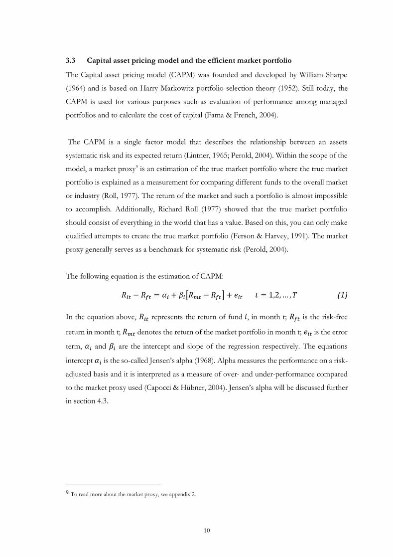
The following equation is the estimation of CAPM:
𝑅𝑖𝑡 − 𝑅𝑓𝑡 = 𝛼𝑖 + 𝛽𝑖[𝑅𝑚𝑡 − 𝑅𝑓𝑡] + 𝑒𝑖𝑡 𝑡 = 1,2,… , 𝑇 (1) In the equation above, 𝑅𝑖𝑡 represents the return of fund 𝑖, in month t; 𝑅𝑓𝑡 is the risk-free
return in month t; 𝑅𝑚𝑡 denotes the return of the market portfolio in month t; 𝑒𝑖𝑡 is the error
term, 𝛼𝑖 and 𝛽𝑖 are the intercept and slope of the regression respectively. The equations
intercept 𝛼𝑖 is the so-called Jensen’s alpha (1968). Alpha measures the performance on a risk-
adjusted basis and it is interpreted as a measure of over- and under-performance compared
to the market proxy used (Capocci & Hübner, 2004). Jensen’s alpha will be discussed further
in section 4.3.
9 To read more about the market proxy, see appendix 2.

11
4 Empirical measurements
4.1 Beta
Beta is a measure of a portfolios systematic risk or volatility in comparison to the market.
The coefficient is calculated with a regression analysis and is based on historical data. A
security’s beta measures how sensitive the security’s return is in comparison to the market.
In the efficient portfolio, the value of beta is assumed to be one (Berk & DeMarzo, 2014).
Therefore, the average asset return moves 1% for each 1% movement in the market. To
clarify, the beta of a security is the expected percentage return change in its return, given a
one-percentage change in the return of the market portfolio (Capocci, 2013).
To calculate an asset’s beta, divide the covariance of the assets return and the benchmark’s
return by the volatility (variance) of the benchmarks return.
𝛽𝑖 =𝑆𝐷(𝑅𝑖) 𝑥 𝐶𝑜𝑟𝑟(𝑅𝑖,𝑅𝑀)
𝑆𝐷(𝑅𝑀) = 𝐶𝑜𝑣(𝑅𝑖,𝑅𝑀)𝑉𝑎𝑟(𝑅𝑀) (2)
Beta, 𝛽𝑖, determines the systematic risk for an investment and [𝑅𝑚 − 𝑅𝑓], which is the risk
premium in the market. By doing so, CAPM can help investors combine a portfolio to
generate the desired expected return (Hamberg, 2001).
4.2 Jensen’s alpha
Jensen’s alpha (1968) is one of the most frequently used measurements when evaluating
hedge fund performance (Jensen, 1968). It is calculated by running equation 1, where Jensen’s
alpha is calculated as:
𝛼𝑖 = 𝑅𝑖𝑡 − (𝑅𝑓𝑡 + 𝛽𝑖(𝑅𝑚𝑡 − 𝑅𝑓𝑡)) (3)
When measuring performance of a hedge fund, or other asset classes, one needs to consider
how much risk a fund contains (Ghysels, Santa-Clara, & Valkanov, 2005). A risk-adjusted
measure is the excess return, calculated as the funds return subtracted with a risk-free
investment, 𝑅𝑓𝑡, of a fund in relation to a selected benchmark. Here, the benchmark is
simply what the fund is supposed to perform under the assumptions of the CAPM (Jensen,
1968; Alexander & Dimitriu, 2005; Sharpe, 1964). The expected alpha of the efficient market
12
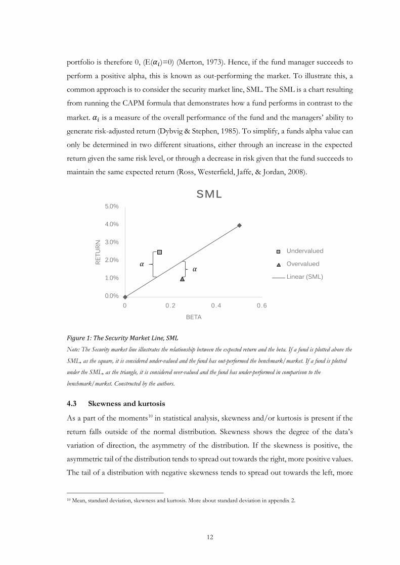
portfolio is therefore 0, (E(𝛼𝑖)=0) (Merton, 1973). Hence, if the fund manager succeeds to
perform a positive alpha, this is known as out-performing the market. To illustrate this, a
common approach is to consider the security market line, SML. The SML is a chart resulting
from running the CAPM formula that demonstrates how a fund performs in contrast to the
market. 𝛼𝑖 is a measure of the overall performance of the fund and the managers’ ability to
generate risk-adjusted return (Dybvig & Stephen, 1985). To simplify, a funds alpha value can
only be determined in two different situations, either through an increase in the expected
return given the same risk level, or through a decrease in risk given that the fund succeeds to
maintain the same expected return (Ross, Westerfield, Jaffe, & Jordan, 2008).
Figure 1: The Security Market Line, SML Note: The Security market line illustrates the relationship between the expected return and the beta. If a fund is plotted above the
SML, as the square, it is considered under-valued and the fund has out-performed the benchmark/market. If a fund is plotted
under the SML, as the triangle, it is considered over-valued and the fund has under-performed in comparison to the
benchmark/market. Constructed by the authors.
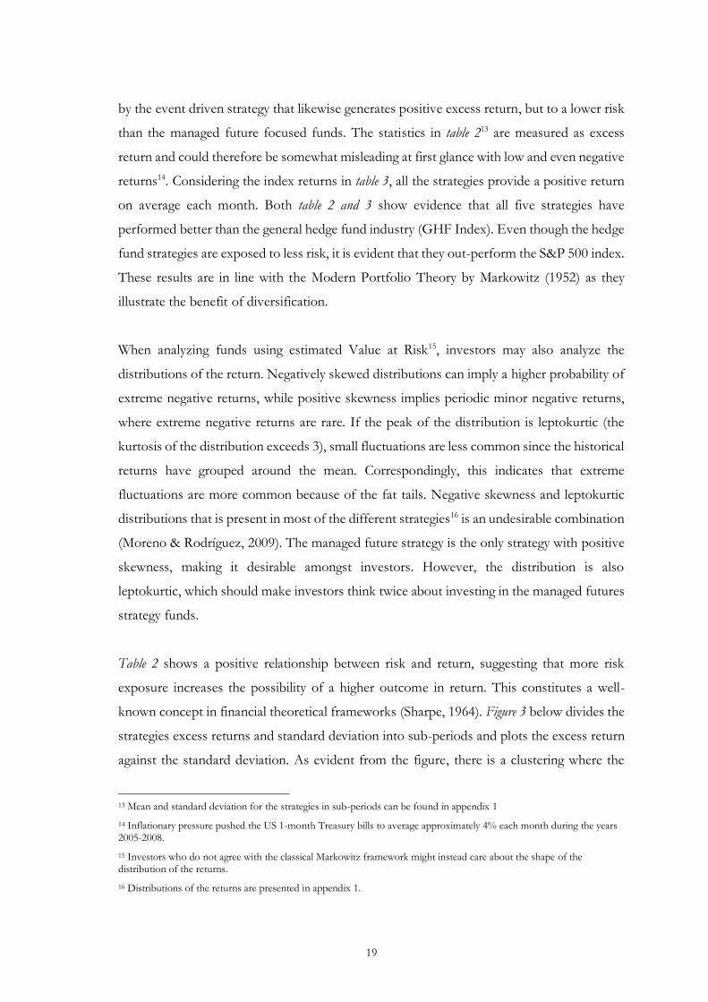
4.3 Skewness and kurtosis
As a part of the moments10 in statistical analysis, skewness and/or kurtosis is present if the
return falls outside of the normal distribution. Skewness shows the degree of the data’s
variation of direction, the asymmetry of the distribution. If the skewness is positive, the
asymmetric tail of the distribution tends to spread out towards the right, more positive values.
The tail of a distribution with negative skewness tends to spread out towards the left, more
10 Mean, standard deviation, skewness and kurtosis. More about standard deviation in appendix 2.
0.0%
1.0%
2.0%
3.0%
4.0%
5.0%
0 0 . 2 0 . 4 0 . 6
RETU
RN
BETA
SML
Undervalued
Overvalued
Linear (SML)𝛼𝛼

13
negative values (left) (Scott & Horvath, 1980). Kurtosis portrays the degree of how peaked
the distribution is. Distributions with a positive kurtosis indicate a peaked distribution, while
negative kurtosis tends to have a flatter distribution (Greene, 2003).
In a normal distribution, the kurtosis equals three. An investment with a high kurtosis will
have a distribution with “fat tails”, both in the negative and positive ends. In addition, high
kurtosis tends to overestimate the likelihood of realizing the mean returns (Connoly &
Hutchinson, 2012).
In investment situations, few returns have normal distributions. Expected returns are often
predicted based on volatility, which are assumed to be normally distributed. By using the
measures of skewness and kurtosis in investment decisions, investors may find more efficient
indicators of the reliability of the investments volatility (Groenveld & Meeden, 1984; Sheikh
& Qiao, 2009) Negative skew Positive skew Positive kurtosis
Figure 2: Skewness and kurtosis distributions Note: figure 2 illustrate three different distributions. Negative skewness (left), have a longer tail to the left and tend to have more n
values that are negative. Positive skewness (middle), have a longer tail to the right and tend to have more values that are positive.
Moreover, the positive kurtosis (right), show the degree of the peak in a distribution. A distribution with greater peak than normal
tend to have higher risk of extreme outcomes. A normal distribution has a skewness value of 0 and kurtosis value of 3.

14
5 Method and data
5.1 Method
The research follows a time-series and comparative research design, that is in accordance
with previous studies (Amenc et al., 2002; Capocci & Hübner, 2004; Eling & Faust, 2010;
Naik et al., 2007). In order to compare hedge fund strategies with a selected benchmark,
which is the measure of what the strategies try to out-perform, the paper uses a quantitative
method. Hedge fund returns are collected as secondary data and statistically analyzed. The
selected time interval is January 2002 to December 2016, which offers a large sample of
returns over a long timespan.
5.2 Sample selection and data collection
The objective of this paper is to examine returns of hedge funds that operate in emerging
markets. All hedge fund data is collected from the Eurekahedge database11, which comprises
a large sample. To be considered an emerging market fund, at least 90% of the funds’ assets
must be allocated in the region. In this research, emerging markets is defined in accordance
with Eurekahedge as the regions: developing Europe (Central and Eastern), Latin America,
Russia, Asia (excluding Japan, Australia and New Zealand), the Middle East, Africa and the
Caribbean (Eurekahedge, 2017).
The hedge fund data regarding emerging markets on Eurekahegde consists of 349 equally
weighted funds, categorized into different strategies. This study includes five strategies and
the selection is described in section 5.3.1 below. Further, the selected benchmark is the
Eurekahedge Hedge Fund index, from now on called the GHF index, which comprises 2797
global hedge funds.
All fund results included in this study are assembled monthly by Eurekahedge and measured
in terms of profit/loss of the whole portfolio worth and are net of fees. There are no “twin”
funds in the benchmark index, e.g. no onshore and offshore type of the same fund. New
funds, with at least a three-month history, are rebalanced into the index while closed funds
historical performance remains permanently.
11 As of March 2017.

15
To calculate the hedge funds risk-adjusted returns, data was collected for the one-month US
Treasury Bill from the Federal Reserve’s database (Federal Reserve, 2017). Lastly, to enable
a comparison between the hedge fund findings and more traditional investment alternatives,
data was collected for the S&P 500 index from Yahoo Finance (Yahoo Finance, 2017).
5.3 Variables
This study includes five different hedge fund strategies to represent the strategy variable. The
five strategies; arbitrage, managed futures, event driven, long/short and fixed income are
selected for their variation in terms of investment characteristics. Some of which are based
on reducing risk and others enhance return by taking higher risks. Arbitrage, long/short and
fixed income are categorized as risk-reducing strategies while managed futures and event
driven enhance risk more frequently (Connor & Woo, 2004). Further, long/short have a style
of taking different positions in the market whereas fixed income locates their investments
into various asset classes, such as currencies and equity (Fung & Hsieh, 1997). The event
driven strategy is based on the managers’ speculation of events that will affect the market.
Lastly, managed futures use sophisticated computer-programs to beat the market (Connor
& Lasarte, 2004).
The benchmark variable is included as a measure to out-perform. As mentioned above it is
the GHF index, which is useful since it provides performance of all underlying funds in the
database, irrespective of region (Eurekahedge, 2017).
5.4 Performance measurement
Together with excess returns, this study will observe the strategies alpha, which measures the
strategies risk-adjusted (systematic risk) performance (Jensen, 1968). Jensen’s alpha is
frequently used in previous research and can illustrate how well a fund performs in
comparison to the benchmark (Capocci & Hübner, 2004; Dichev & Yu, 2011; Eling, 2009;
Eling & Faust, 2010; Fung & Hsieh, 2004; Liang, 1999)
5.5 Data analysis
To evaluate the strategies performance, several regressions were run using the CAPM. All
regressions were treated with a heteroscedasticity and autocorrelation consistent covariance
matrix, which accounts for potential autocorrelation and heteroscedasticity in the data

16
(Newey & West, 1986; Greene, 2003). In addition, an augmented Dickey Fuller test was
conducted to determine if non-stationarity was present.
Besides running regressions on the dataset for each strategy, the time period was divided into
sub-periods, which enabled rolling regressions and thereby increased number of results to
analyze. The complete dataset for each strategy contains 180 months and every sub-period
48 months, with a 24-month overlap for each period. The last sub-period contains 36
observations. The null hypothesis, H0, for all regressions is expressed as alpha equals zero.
In accordance with previous studies, the regressions are performed with significance levels
of 1%, 5% and 10% (Capocci & Hübner, 2004; Eling, 2009; Eling & Faust, 2010).
5.6 Quality of method
The entire dataset in this study is secondary and collected through publicly accessible
databases. Therefore, there is limited control over the quality. Since hedge funds are not
required to report historical performance, the collected data might not be unbiased and this
is a disadvantage of this type of information that one should be aware of when analyzing the
results (Fung & Hsieh , 2000). Further, the data is hand collected by the authors and thereby
carries the risk of human error.
The strategies were selected because of their diversity. However, there are more strategies in
emerging markets and arguments could be made to suggest another combination of strategies
based on different selection criteria. The data available for hedge funds is efficient to interpret
using the CAPM, which generates desired estimations. The model has however been
criticized for being simplistic and academic studies regarding hedge funds often add other
performance measurement models to further analyze the variety in fund returns (Agarwal &
Naik, 2000; Capocci & Hübner, 2004; Eling & Faust, 2010; Fama & French, 2004; Liang,
1999). Since alpha is determined in proportion to a benchmark assessed as suitable for the
fund, it is important that the chosen benchmark is representative, otherwise one can draw
misleading conclusions (CFA Institute, 2013).
5.7 Potential biases
Eurekahedge is a well-established database that covers numerous hedge funds (Capocci,
2013). The data might suffer from three potential biases, namely; backfilling bias,
survivorship bias and selection bias (Fung & Hsieh , 2000). Backfilling bias occurs when a

17
new hedge fund is added to the database and is asked to provide historical performance.
Hedge fund managers could for instance refuse to provide performance history if the result
is poor. In contrast, managers also have strong incentives to overestimate their performance
since this could bring more clients. This line of reasoning suggests that only managers with
a good track record has the incentive to backfill their past performance which could lead to
a bias (Eling & Faust, 2010). However, this problem could be solved by simply subtracting
the past 12-24 monthly returns of the recently added funds (see Fung & Hsieh , 2000;
Capocci & Hübner, 2004). Eling (2009) concluded that this technique would decrease the
monthly return by 0.18 % on average while Fung and Hsieh (2000) reported that the monthly
return would decrease by 0.12 % on average.
Funds are considered dead or closed when they stop reporting their performance to various
databases (Eurekahedge, 2017). There are various reasons for this, but the most likely one is
poor performance. Survivorship bias is when a fund’s assets only contain those investments
that have been successful in previous periods. Several failing and closed funds are merged
into other funds to cover weak performance (Fung & Hsieh , 2000). The Eurekahedge
database attempt to solve this problem by letting the past performance of the closed funds
be a part of the indices. In this way, the impact of the survivorship bias in this study should
not be of great concern (Eling & Faust, 2010).
Hedge funds are included in the category of special funds and reporting data is voluntary for
the managers. This could lead to selection bias. Given the choice to present your past
performance or not, it makes sense that with a good track record one would be more willing
to do so. In the same way, it makes sense to not present past performance if a manager
constantly under-performs (Eling & Faust, 2010). Further, Fung and Hsieh (1997) state that
the selection bias should be of minor concern since a significant number of well performing
funds are uninterested in new investors and additional capital because new capital make the
funds returns decrease to a certain level12.
12 Additional financing to the fund result in less opportunities to find lucrative investments. Hence, more capital inflow will make returns decline until they are no longer profitable (Berk & Green, 2004).

18
6 Empirical results
6.1 Descriptive statistics
The descriptive statistics presented table 2 represent the moments, mean, standard deviation,
skewness and kurtosis of the distribution for the five strategies, the benchmark and the S&P
500. The table also contains information on the minimum and maximum values of each
variable.
Table 2: Descriptive statistics: monthly excess returns for strategies, GHF index and the S&P 500
Note: All statistics are analyzed as monthly excess returns. Descriptive statistics for each strategy, the GHF index and the S&P 500 are calculated as average values from January 2002 to December 2016. The four moments mean, standard deviation, skewness and kurtosis together with minimum and maximum values are presented.
Table 3: Descriptive statistic: monthly returns for strategies, GHF index and the S&P 500
Note: All statistics are analyzed as monthly returns. Descriptive statistics for each strategy, the GHF index and the S&P 500 are calculated as average values from January 2002 to December 2016. The four moments mean, standard deviation, skewness and kurtosis together with minimum and maximum values are also presented. To achieve an unbiased comparison, all the measures are calculated with an equally weighted
average (Capocci & Hübner, 2004). The strategies vary in return and this suggest that
managed futures are the strategy that generates the highest returns on average each month,
as well as the highest maximum value (19.84 %). Further, managed futures are the strategy
that takes the most risk and is the most volatile among the different strategies. It is followed
Mean (%) Std. Dev. (%) Skewness Kurtosis Min (%) Max (%)GHF index -0,51 1,94 -0,58 0,20 -5,98 4,90Arbitrage -0,37 1,60 -0,73 -0,07 -4,39 2,95Managed futures 0,18 4,33 0,57 4,67 -14,60 19,84Event driven 0,05 3,57 -0,02 2,23 -11,73 14,78Long/Short -0,19 3,36 -0,42 1,16 -11,42 10,78Fixed Income -0,48 2,05 -0,75 1,21 -9,33 4,36S&P 500 -0,72 4,48 -0,33 0,65 -17,20 10,76
Mean (%) Std. Dev. (%) Skewness Kurtosis Min (%) Max (%)GHF index 0,67 1,38 -0,49 1,53 -4,48 5,04Arbitrage 0,81 0,83 -0,43 1,63 -2,32 2,95Managed futures 1,36 3,82 1,56 6,86 -9,49 21,49Event driven 1,23 3,44 -0,04 3,23 -11,47 16,43Long/Short 0,99 3,25 -0,53 1,23 -11,16 10,92Fixed income 0,70 1,50 -2,03 10,44 -9,07 4,50S&P500 0,46 4,14 -0,69 1,68 -16,94 10,77
19
by the event driven strategy that likewise generates positive excess return, but to a lower risk
than the managed future focused funds. The statistics in table 213 are measured as excess
return and could therefore be somewhat misleading at first glance with low and even negative
returns14. Considering the index returns in table 3, all the strategies provide a positive return
on average each month. Both table 2 and 3 show evidence that all five strategies have
performed better than the general hedge fund industry (GHF Index). Even though the hedge
fund strategies are exposed to less risk, it is evident that they out-perform the S&P 500 index.
These results are in line with the Modern Portfolio Theory by Markowitz (1952) as they
illustrate the benefit of diversification.
When analyzing funds using estimated Value at Risk15, investors may also analyze the
distributions of the return. Negatively skewed distributions can imply a higher probability of
extreme negative returns, while positive skewness implies periodic minor negative returns,
where extreme negative returns are rare. If the peak of the distribution is leptokurtic (the
kurtosis of the distribution exceeds 3), small fluctuations are less common since the historical
returns have grouped around the mean. Correspondingly, this indicates that extreme
fluctuations are more common because of the fat tails. Negative skewness and leptokurtic
distributions that is present in most of the different strategies16 is an undesirable combination
(Moreno & Rodríguez, 2009). The managed future strategy is the only strategy with positive
skewness, making it desirable amongst investors. However, the distribution is also
leptokurtic, which should make investors think twice about investing in the managed futures
strategy funds.
Table 2 shows a positive relationship between risk and return, suggesting that more risk
exposure increases the possibility of a higher outcome in return. This constitutes a well-
known concept in financial theoretical frameworks (Sharpe, 1964). Figure 3 below divides the
strategies excess returns and standard deviation into sub-periods and plots the excess return
against the standard deviation. As evident from the figure, there is a clustering where the
13 Mean and standard deviation for the strategies in sub-periods can be found in appendix 1 14 Inflationary pressure pushed the US 1-month Treasury bills to average approximately 4% each month during the years 2005-2008. 15 Investors who do not agree with the classical Markowitz framework might instead care about the shape of the distribution of the returns. 16 Distributions of the returns are presented in appendix 1.

20
standard deviation is low. When there is a systematic increase in the standard deviation, the
returns are more “spread” and vary significantly more17.
Figure 3: Combinations of risk and return for hedge funds
Note: Illustration of the combination between risk and return for hedge funds. The figure show that hedge funds with lower standard
deviation have more concentrated low returns. Returns are more “spread out” as standard deviation increase. Hence, by taking
more risk higher returns may be possible, but may also lead to bigger losses.
6.2 Correlation
Research regarding hedge funds suggests that hedge funds improve the trade-off between
risk and return in a portfolio due to their weak correlation with other securities (Fung &
Hsieh, 1997; Liang, 1999). However, Eling and Faust (2010) found that hedge funds and
mutual funds had a correlation coefficient of 0.91, but hedge funds generated higher alpha
values than the mutual funds. One of the main arguments when advocating for investments
in hedge funds is that their correlation with traditional investments is somewhat low, which
makes hedge funds favorable for diversification purposes (Capocci & Hübner, 2004; Eling
& Faust, 2010).
17 The relationship between risk and return can be somewhat clearer when the graph is plotted with absolute values instead of excess returns which is shown in appendix 1.
-8
-6
-4
-2
0
2
4
0 1 2 3 4 5 6 7 8
Exce
ss re
turn
(%)
Standard deviation (%)

21
Table 4: Correlation between the GHF index, hedge fund strategies and the S&P 500
*** Correlation is significant at 1% Note: table 4 illustrate the correlation coefficients between the GHF index, the five strategies and the S&P 500 index, measured from January 2002 to December 2016. Correlation coefficients values fall between -1 and 1. Positive correlation coefficients indicate that securities move in same directions and negative correlation coefficient indicate that securities move in opposite directions.
In table 4 the correlation of this study’s benchmark: GHF index, the five strategies and the
S&P 500 index, from January 2002 to December 2016 is presented. As evident from the
table, the variability between the different strategies is high, ranging from 0.847 (between
long/short and event driven) – to 0.044 (between managed futures and event driven).
Regarding the managed futures, the results show that this strategy has a lower correlation
coefficient with the other strategies and both indices. In addition, the managed futures’
correlation coefficient is insignificant in three of the cases (with event driven, long/short and
the S&P 500). The GHF index has a high correlation (over 0.70) with four out of five
strategies and the S&P 500. Ranging in variability from 0.882 (with fixed income) – to 0.349
(with managed futures). The GHF index and S&P 500 correlation coefficient equals 0.748.
Although there is relatively high correlation amongst the GHF index and S&P 500, all five
strategies are more correlated with the GHF index.
6.3 Performance measurement results
The data provided in table 518 comprises the alphas obtained from the CAPM-regression for
the five strategies together with a 95% confidence interval. They are presented over the entire
observation period as well as in sub-periods in order to interpret how they have performed
18 The regressions where made using a heteroscedasticity and autocorrelation consistent
Covariance matrix (Newey & West, 1986; Greene, 2003).
GHF index ArbitrageManaged
futuresEvent driven
Long/shortFixed
incomeS&P 500
GHF index 1Arbitrage ,794** 1Managed futures
,349** ,451** 1
Event driven ,701** ,449** ,044 1Long/short ,814** ,476** ,143 ,847** 1
Fixed income ,882** ,773** ,287** ,705** ,764** 1
S&P 500 ,748** ,492** ,109 ,622** ,724** ,690** 1

22
and changed during the time interval. Additionally, table 5 presents both the beta and
adjusted 𝑅2 values19.
When running the regression in sub-periods, approximately 60% of the significant hedge
fund strategies produce positive alphas and therefore succeeds to out-perform the
benchmark. This finding implies that hedge fund managers who allocate their assets in
emerging markets on average perform better than managers who place their assets in
developed economies. The managed futures, event driven and long/short strategies succeed
to generate positive alphas during the whole period from January 2002 until December 2016,
meaning that these strategies significantly out-perform the main hedge fund index. The
obtained adjusted R-square values that lies around 0.5-0.6 are in line with other research
(Eling & Faust, 2010), with the managed futures as an exception.
The results in table 5 indicate that the arbitrage strategy appears to be affected by the general
market environment, as it generates negative and insignificant alphas during periods of
uncertainty, meaning that they performed in a way statistically indistinguishable from the
benchmark. In times of growth, the arbitrary strategies manage to create positive alphas.
From January 2008 to December 2013, it generates insignificant positive alphas, however,
these alphas lower confidence intervals are close to zero. Figure 4 below clarifies how the
different alphas have moved during the period of study and from this it is clear that the
arbitrage strategy has experienced a substantial increase in performance during the past years.
The arbitrary strategies beta values shown in figure 5, are also subject to a decrease throughout
the same period and could constitute a possible explanation. The efficient market hypothesis
alludes that with perfect information in the financial markets, the market will be efficient and
out-performing the market will be impossible. Those strategies that generate return on
market inefficiencies, like the arbitrary strategies, are able to out-perform the benchmark
extensively. They thereby prove that financial emerging markets are inefficient and react
slowly to information.
19 In the context of evaluating the CAPM, an adjusted R-square of 0.7 states that 70% of the funds’ performance is described
by its risk exposure, its beta. And the other 30% can be seen as the manager’s skill or pure luck. Hence, in the CAPM, the
only term that is adjusted for is the market variable,[𝑅𝑚 − 𝑅𝑓] (Eun, Resnick, & Sabherwal, 2012)

23
Table 5: Regression result of the CAPM showing alpha, beta and adjusted R-square
Strategy α Lower 95% Upper 95% β
Arbitrage
January 2002-December 2016 -0,04 -0,22 0,14 0,65 *** 0,63January 2002-December 2005 -0,17 -0,55 0,22 0,56 ***January 2004-December 2007 -0,69 *** -1,28 -0,10 0,68 ***January 2006-December 2009 -0,47 *** -0,86 -0,09 0,64 ***January 2008-December 2011 0,17 -0,05 0,38 0,42 ***January 2010-December 2013 0,13 -0,09 0,34 0,48 ***January 2012-December 2015 0,52 *** 0,14 0,89 0,13January 2014-December 2016 0,67 *** 0,34 0,99 -0,11
Managed futures
January 2002-December 2016 0,58 * -0,05 1,22 0,78 *** 0,12January 2002-December 2005 0,45 -0,45 1,35 0,40January 2004-December 2007 -0,82 -2,51 0,87 0,97 ***January 2006-December 2009 0,87 -1,27 3,00 1,04 ***January 2008-December 2011 2,23 *** 0,80 3,66 0,21January 2010-December 2013 0,98 *** 0,29 1,68 0,12January 2012-December 2015 0,73 ** 0,12 1,35 0,02January 2014-December 2016 0,66 * -0,07 1,39 0,26
Event driven
January 2002-December 2016 0,71 *** 0,24 1,18 1,29 *** 0,49January 2002-December 2005 2,21 *** 1,10 3,32 1,85 ***January 2004-December 2007 1,79 *** 0,74 2,84 1,29 ***January 2006-December 2009 0,75 *** 0,24 1,26 1,21 ***January 2008-December 2011 -0,25 -0,62 0,11 1,61 ***January 2010-December 2013 -0,42 * -0,94 0,10 1,82 ***January 2012-December 2015 -0,29 -0,81 0,23 1,99 ***January 2014-December 2016 0,10 -0,33 0,53 1,67 ***
Long/Short
January 2002-December 2016 0,53 *** 0,16 0,90 1,41 *** 0,66January 2002-December 2005 1,35 *** 0,79 1,91 1,67 ***January 2004-December 2007 1,71 *** 0,89 2,53 1,32 ***January 2006-December 2009 1,29 *** 0,41 2,17 1,46 ***January 2008-December 2011 -0,42 *** -0,79 -0,05 2,01 ***January 2010-December 2013 -0,59 *** -0,95 -0,23 1,97 ***January 2012-December 2015 -0,33 -0,78 0,11 2,03 ***January 2014-December 2016 -0,20 -0,76 0,35 2,13 ***
Fixed income
January 2002-December 2016 0,00 -0,17 0,16 0,93 *** 0,78January 2002-December 2005 -0,03 -0,28 0,22 0,73 ***January 2004-December 2007 -0,51 *** -0,98 -0,04 0,80 ***January 2006-December 2009 -0,09 -0,43 0,25 0,96 ***January 2008-December 2011 0,17 -0,15 0,50 0,97 ***January 2010-December 2013 -0,01 -0,39 0,38 0,95 ***January 2012-December 2015 -0,25 * -0,63 0,13 1,03 ***January 2014-December 2016 0,05 -0,31 0,41 0,86 ***
𝑅𝑎 2
Note: Table 5 present the five strategies alpha and beta values from January 2002 to December 2016 together with seven sub-periods. Also included the alphas confidence intervals at 95% and each strategies Adjusted R-squared.
* Indicates significance at 10% level ** Indicates significance at 5% level *** Indicates significance at 1% level

24
Managed futures succeed to generate positive alpha values in most sub-periods except for
the period between 2004 and 2007. Even though the first three sub-periods are insignificant
and have a wide confidence interval, it could be argued that the managed futures perform
well when the other strategies do not. This is confirmed in figure 4. As illustrated in table 4,
managed futures is the strategy that is the least correlated with both the S&P 500 and the
GHF index. The vague relationship between the methods practiced by the managed futures
managers’ and the financial market allows this type of strategy to generate positive alphas in
both falling and rising markets. The alphas of the managed futures strategy funds have
declined systematically over the past years, leaving the question if this strategy’s performance
measurement will continue to decline.
Given a correlation coefficient of 0.847 and as figure 4 illustrates, the event driven and
long/short funds tend to move in the same direction. The event driven and the long/short
strategies both have significant positive alphas in the beginning of the studied period. In
addition, the event driven strategy generates the highest significant alpha during the full study
period. According to the efficient market hypothesis, the only way of achieving greater
returns than the market is by acquiring more risky assets. Both strategies are subject to high
beta values, as can be seen in figure 5; they are also the two strategies that are exposed to the
most systematic risk. In the later periods however, none of the alphas are significantly
different from zero.
Event driven strategies and long/short strategy funds creates positive alphas in periods of
uncertainty and fluctuating markets20. A bold explanation for this might be that these
strategies try to benefit from mispriced market events, such as profit warnings and takeovers,
which occur frequently during volatile stages. On the other hand, it can help describe why
the two strategies fail to continue generating positive alphas during market neutral
conditions. The fixed income strategy funds generate alphas of around 0, and only produces
two significant values that are negative, occurring during the periods January 2004 to
December 2007 and January 2012 to December 2015. These findings suggest that the fixed
income strategy fails to perform better than the global hedge fund market. Fixed income
20 Fluctuating and market neutral markets are in this context referred to periods when the standard deviation of the main hedge fund index and the S&P 500 have a high and low standard deviation respectively. See tables for standard deviation in appendix 2.

25
focuses mostly on relatively reliable returns, given that they take on almost the same risk,
beta, as the global hedge fund market, it is no surprise that they perform approximately the
same as GHF index.
Figure 4: The change in estimated alpha from January 2002 to December 2016
Note: Figure 4 illustrate the movement of the estimated alpha values for the arbitrage, managed futures, event driven, long/short and fixed income strategies from January 2002 to December 2016. Alpha values above zero indicate that the strategy have performed better than the benchmark/market, and alpha values below zero indicate that the strategy have performed worse than the benchmark/market.
Figure 5: The change in estimated beta from January 2002 to December 2016
Note: Figure 5 illustrate the movement of the estimated beta values for the arbitrage, managed futures, event driven, long/short and fixed income strategies from January 2002 to December 2016. Beta measure the strategies systematic risk, their sensitivity to changes in the market.
-1
-0.5
0
0.5
1
1.5
2
2.5
Estim
ated
Alp
ha
Arbitrage Managed futures Event driven Longshort Fixed income
-0.5
0
0.5
1
1.5
2
2.5
Estim
ated
Bet
a
Arbitrage Managed futures Event driven Longshort Fixed income
2002 2016
2002 2016

26
Fung and Hsieh (2011) and Fung et al. (2008) found a downward trend in the generated
alphas in emerging markets at the end of their investigation period. Strömqvist (2007)
however suggest that emerging market hedge funds should generate positive alphas in the
future. This statement is neither confirmed nor rejected based on the results of this study.
According to results in table 5 and figure 4 this seems to be true regarding the strategy managed
futures, which produces positive significant alphas over the four last periods, indicating an
out-performance of the benchmark. This also seems to be true for arbitrage funds that
succeed to generate positive significant alphas the last two periods. The other strategies either
under-perform or have insignificant alphas throughout the same periods. Contradictory to
the research by Strömqvist (2007), Abugri and Dutta (2009) and Eling, and Faust (2010)
declares that managers of emerging market hedge funds have changed their investment
behavior after 2006, and from that period onwards show a similar pattern as the one recorded
for advanced market hedge funds. Abugri and Dutta’s (2009) study is based on the entire
emerging market hedge fund industry and argues that this industry does not out-perform the
benchmarks on a regular basis after 2006. This argument is consistent with the results in this
study, with the exception that this study suggest that this situation starts in 2008, at least
regarding the event driven, long/short and fixed income strategy who all produce close to
benchmark and even negative alphas constantly after that period.
6.4 Performance in different market environments
According to table 5 the arbitrage strategy is affected by the general market environment and
tends to produce positive alphas when the market is in a positive trend, whilst it tends to
perform negative alphas when the economy is in a negative trend. In comparison, the
managed futures strategy seems to be somewhat unaffected by both the GHF index and the
S&P 500 and manages to perform positive alphas regardless of the economic environment.

27
Figure 6: Strategy returns in different environments Note: Figure 6 illustrate the five observed strategies, GHF main index, and S&P 500’s performance in four different market
environments. Environment 1 represents each observation 45 worst months on average returns and environment 4 represents the
observations 45 best months on average returns.
To further investigate the question, figure 6 contains a graph that presents the different
strategies, the benchmark and the S&P 500 and their excess returns in different market
environments. The excess returns are divided into four different market environments to
sort out the peaks and troughs for each individual strategy. The market situations are ranked
from 1 to 4, where 1 is the average excess returns of the 45 lowest performing months and
4 is the average excess return of the 45 highest performing months for each strategy. Due to
high correlation, it is no surprise that the fixed income strategy achieves the most similar
returns to the GHF index in the different environments. As for the event driven strategy,
long/short strategy and the S&P 500, the returns look similar in three out of the four periods.
According to Eling and Faust (2010), hedge fund managers shift their allocations and adapt
to changing market environments earlier than the regular investor. This result is found also
in this study and is evident from figure 6, where all the hedge funds and the benchmark
succeeds already in market environment 2 to generate a positive return, whilst the S&P 500
still suffers from negative average excess returns.
-6
-4
-2
0
2
4
6
1 2 3 4
Aver
age
retu
rn
Arbitrage
Fixed income
Global main index
Long/Short
Event driven
S&P 500
Managed futures

28
Table 5 presents the betas of the different strategies in comparison to their benchmark, the
GHF index. The strategies long/short and event driven have significant betas of over 1
during the entire period. Asserting that they should perform better than their benchmark
during their best environments and perform worse during their worst environment,
something that is confirmed in figure 6. Regarding the managed futures, there are a lot of
betas that are not significant; hence it is difficult to explain why the managed futures perform
so well during the good periods and bad during the bad periods. Another interesting finding
is that the arbitrage strategy seems to succeed in fulfilling its purpose of being a risk-reducing
strategy. It generates the least negative return during market environment 1 and offers, at
least to some degree, downside security in harmful market environments. Hence, in figure 6,
it is possible to identify a connection between risk and return as the strategies (managed
futures, event driven and long/short) who take on most risk seems to perform worst during
bad periods and best during good periods.

29
7 Conclusion
This paper investigates whether emerging market hedge funds perform better than the global
hedge fund market and questions previous research that does not distinguish between
different strategies when studying emerging market hedge funds (Abugri & Dutta, 2009;
Eling & Faust, 2010; Fung & Hsieh, 2006). In terms of risk-adjusted return, it is evident from
the results that all emerging market hedge fund strategies out-perform the GHF index during
the whole investigation period. Ackermann et al. (1999), Liang (1999), Capocci and Hübner
(2004) amongst others, state that hedge funds serve as an excellent investment for
diversification purposes. In this study, returns of the emerging market hedge funds are higher
than the alternative investment S&P 500, even though they are subject to less risk. This result
is in line with the Modern Portfolio Theory by Markowitz (1952) that emphasizes the
importance of diversification in a portfolio. The results from the regression of the CAPM
are a bit contradicting, as they conclude that the obtained positive alphas of the regressions
indicate that 60% of the strategies in the emerging market hedge funds perform better than
the GHF index.
Additionally, this paper examines if there is a difference in performance depending on what
strategy the fund managers’ practice. One key finding of the research is the difference in
performance that each strategy delivers, and displays the importance of dividing funds into
strategies rather than focusing on the degree of development in that market. This paper
concludes that arbitrage strategy funds offer, at least to some degree, downside security in
harmful market environments and is therefore superior for hedging purposes. Strategies with
a focus on arbitrary gains have performed better than the benchmark during January 2008 to
December 2016, which would not be possible under the efficient market hypothesis if
financial markets were efficient. The reason for emerging markets being less efficient is
usually denoted as a main reason for why they should generate higher returns than developed
markets. This paper finds evidence supporting this during the last periods.
For performance purposes, there are two possible ways to determine what strategy that is
superior. Based on the findings from the full investigation period, it seems that the event
driven strategy is the superior as it generates the highest performance. This way of
determining the overall performance might be misleading since in the first half of the

30
investigation period, it is evident that two strategies event driven and long/short strategies
shared this position, whereas managed futures is superior from January 2008 and onwards.
An augmented Dickey Fuller test showed a problem with stationarity in the arbitrage strategy
in the CAPM regression conducted. This could have been triggered by a structural break and
makes the conclusion of that strategy less precise. Contradictory, the other strategies
displayed no problems with stationarity. Hedge fund performance could be investigated in
several ways. The correlation with the GHF index and the Adjusted R-squared regarding the
managed futures strategy are low, implying that there are other elements that determine the
return for this strategy. Agarwal and Naik (2004), Capocci and Hübner (2004) and Eling and
Faust (2010) showed that multifactor models increase the Adjusted R-squared values and the
use of these models might explain the variation in risk-adjusted return for the managed
futures strategy better. However, one cannot reject that the generated return for hedge funds
could depend on managerial skill as well.
7.1 Future research
A compelling application of further research would be to examine more strategies and what
additional factors that determine performance of emerging market hedge fund strategies,
rather than just a risk factor derived from a benchmark. This could be done using the
multifactor models previously mentioned. Eling and Faust (2010) conclude in their study
that multifactor models help explain the variation in return for emerging market hedge funds
better than the CAPM. Analysis of what factors determine the shift in investor behavior
during the last decade could provide further insight regarding what creates return in both
times of economic contraction and expansion. (Ratner & Leal, 2005)

31
References
Abugri, B. A., & Dutta, S. (2009). Emering market hedge funds: Do they perform like regular
hedge funds? Journal of International Financial Markets, Institutions and Money, 19(5), 834-
849.
Ackermann, C., Richard, M., & Ravenscraft, D. (1999, June). The Performance of Hedge
Funds: Risk, Return, and Incentives. The Journal of Finance, 54(3), pp. 833-874.
Agarwal, V., & Naik, N. Y. (2000). On Taking the ‘Alternative' Route: Risks, Rewards and
PerformancePersistence of Hedge Funds. The Journal of Alternative Investments, 2(4), 6-
23.
Agarwal, V., & Naik, N. Y. (2004). Risk and Portfolio Decision Involving Hedge Funds. The
Review of Financial Studies, 17(1), 63-98.
Alexander, C., & Dimitriu, A. (2005). Rank alpha funds of hedge funds. The Journal of
Alternative Investments, 8(2), 48-61.
Amenc, N., & Martellini, L. (2002). Portfolio optimization and hedge fund style allocation
decisions. The Journal of Alternative Investments, 5(2), pp. 7-20.
Amenc, N., Martellini, L., & Vaissié, M. (2002). Benefits and Risks of Alternative Investment
Strategies. Journal of Asset Management, 4(2), 96-118.
Amin, G. S., & Kat, H. M. (2001). Welcome to the dark side: Hedge fund attrition and
survivorship bias over the period 1994–2001. The Journal of Alternative Investments, 6(1),
57-73.
Amin, G. S., & Kat, H. M. (2003). Stocks, bonds, and hedge funds. The journal of portfolio
Management, 29(4), 113-120.
Basu, A. K., & Huang-Jones, J. (2015). The performance of diversified emerging market
equity funds. Journal of International Financial Markets, Institutions & Money, 35, pp. 116-
131.
Bekaert, G., & Harvey, C. R. (2002). Research in emerging markets finance: looking to the
future. Emerging Markets Review, 3, pp. 429–448.
Berk, J. B., & Green, R. C. (2004). Mutul Fund Flows in Rational Markets. Journal of Political
Economy, 1269-1295.
Berk, J., & DeMarzo, P. (2014). Corporate Finance. Harlow, England: Pearson Education Ltd.

32
Brown, S. J., Goetzmann, W. N., & Ibbotson, R. G. (1999). Offshore Hedge Funds: Survival
& Performance 1989 - 1995. The Journal of Business, 72(1), 91-117.
Capocci, D. (2013). The Complete Guide to Hedge Funds and Hedge Fund Strategies. London :
Palgrave Macmillan.
Capocci, D., & Hübner, G. (2004). Analysis of hedge fund performance. Journal of Empirical
Finance, 11, pp. 55-89.
CFA Institute. (2013). Portfolio Management. In Corporate Finance, Potfolio Management, and
Equity Investments (pp. 125-197). Kaplan Inc.
Clarke, J., Jandik, T., & Mandelker, G. (2001). The efficient markets hypothesis. In Expert
financial planning: Advice from industry leaders (pp. 126-141).
Connoly, C., & Hutchinson, M. C. (2012). Dedicated Short Bias Hedge Funds:
Diversification and Alpha during Financial Crises. The Journal of Alternative Investments,
14(3), 28-41.
Connor, G., & Lasarte, T. (2004). An Introduction to Hedge Fund Strategies. In Introducutory
Guide. London: International Asset Management, London School of Economics and
Political Science.
Connor, G., & Woo, M. (2004). An Introduction to hedge funds. Financial Markets Group,
London School of Economics and Political Science.
Datastream. (2017, May 10). Thomson Reuters Datastream. Retrieved from Thomson Reuters
Datastream: Subscription Service
Dichev, I. D., & Yu, G. (2011). Higherrisk,lowerreturns:Whathedgefundinvestorsreallyearn.
JournalofFinancialEconomics, 100, 248-263.
Dybvig, P. H., & Stephen, R. A. (1985). Differential information and performance
measurement using a security market line. The Journal of finance, 40(2), 383-399.
Edwards, F. R., & Caglayan, M. O. (2001). Hedge fund performance and manager skill.
Journal of Futures Markets, 21(11), 1003-1028.
Eling, M. (2009, August). Does Hedge Fund Performance Persist? Overview and New
Empirical Evidence. European Financial Management.
Eling, M., & Faust, R. (2010). The performance of hedge funds and mutual funds in emerging
markets. Journal of Banking & Finance, 34, pp. 1993-2009.
Elton, E. J., & Gruber, M. J. (1997). Modern portfolio theory, 1950 to date. Journal of Banking
& Finance, 21, pp. 1743-1759.

33
Eun, C. S., Resnick, B. G., & Sabherwal, S. (2012). International Finance. New York: McGraw-
Hill/Irwin.
Eurekahedge. (2017). Eurekahedge. Retrieved from Indices - Eurekahedge Equal Weighted
Hedge Fund Index: http://www.eurekahedge.com/Indices/hedge-fund-index-
methodology
Fama , E. F. (1970, May). Efficient Capital Markets: A Review of Theory and Empirical
Work . The Journal of Finance, 25(2), pp. 383-417.
Fama, E. F., & French, K. R. (2004, Summer). The Capital Asset Pricing Model: Theory and
Evidence. Journal of Economic Perspectives, 18(3), pp. 25-46.
Fama, E. F., & French, K. R. (2012). Size, value, and momentum in international stock
returns. Journal of financial economics, 105(3), 457-472.
Federal Reserve. (2017). Board of Governors of the Federal Reserve System. Retrieved from Board
of Governors of the Federal Reserve System: https://www.federalreserve.gov/
Ferson, W. E., & Harvey, C. R. (1991). The Variation of Economic Risk Premiums. Journal
of Political Economy, 99(2), 385-415.
Fung, W., & Hsieh , D. A. (2000, September). Performance Characteristics of Hedge Funds
and Commodity Funds: Natural vs. Spurious Biases. Journal of Financial and Quantitative
Analysis, 35(3), pp. 291-307.
Fung, W., & Hsieh, D. A. (1997). Empirical Characteristics of Dynamic Trading Strategies:
The Case of Hedge Funds. The Review of Financial Studies, 10(2), pp. 275–302.
Fung, W., & Hsieh, D. A. (2001). The Risk in Hedge Fund Strategies: Theory and Evidence
from Trend Followers. Review of Financial Studies, 14(2), pp. 313-341.
Fung, W., & Hsieh, D. A. (2004). Hedge Fund Benchmarks: A Risk-Based Approach.
Financial Analysts Journal, 60(5), 65-80.
Fung, W., & Hsieh, D. A. (2006). Hedge funds: an industry in its adolescence. Economic Review-
Federal Reserve Bank Of Atlanta, 91(4), 1-33.
Fung, W., & Hsieh, D. A. (2011). The risk in hedge fund strategies: Theory and evidence
from long/short. Journal of Empirical Finance, 18, 547-569.
Fung, W., Hsieh, D. A., & Tsatsaronis, K. (2000). Do Hedge Funds Disrupt Emerging
Markets? Brooking-Wharton Papers on Financial Services, 377-401.
Fung, W., Hsieh, D. A., Naik , N. Y., & Ramadorai, T. (2008). Hedge funds:
Performance,risk, and capital formation. Journal of Finance, 63(4), 1777–1803.

34
Ghysels, E., Santa-Clara, P., & Valkanov, R. (2005). There is a risk-return trade-off after all.
Journal of Financial Economics, 76(3), 509-548.
Greene, W. H. (2003). Econometric analysis. Pearson Education.
Groenveld, R. A., & Meeden, G. (1984). Measuring Skewness and Kurtosis. The Statistician,
391-399.
Hamberg, M. (2001). Strategic Financial Decisions. Sweden: Liber AB.
Jensen, M. C. (1968). The Performance of Mutual Funds in the Period 1945-1964. Journal of
Finance, 389-416.
Law, J. (2009). Dictionary of business and management. Oxford: Oxford University Press.
Lazard Asset Management. (2014). Emerging Markets Hedge Funds: Capturing Alpha in an
Inefficient Asset Class. Lazard Asset Management.
Liang, B. (1999). On the Performance of Hedge Funds. Financial Analysts Journal, pp. 72–85.
Liang, B. (2000). Hedge funds: The living and the dead. Journal of Financial and Quantitative
analysis, 35(3), pp. 309-326.
Lintner, J. (1965). The Valuation of Risk Assets and the Selection of Risky Investments in
Stock Portfolios and Capital Budgets. The Review of Economics and Statistics, 47(1), 13-
37.
Lo, A. W., Repin, D. V., & Steenbarger, B. N. (2005). Fear and greed in financial markets: A
clinical study of day-traders. National Bureau of Economic Research.
Markowitz, H. (1952, March). Portfolio Selection. The Journal of Finance, 7(1), pp. 77-91.
Merton, R. C. (1973). An Intertemporal Capital Asset Pricing Model. Econometrica: Journal of
the Econometric Society, 867-887.
Moreno, D., & Rodríguez, R. (2009). The value of coskewness in mutual fund performance
evaluation. Journal of Banking & Finance, 33(9), 1664-1676.
Mossin, J. (1966). Equilibrium in a Capital Asset Market. Econometrica, 34(4), 768-783.
Naik, N. Y., Ramadorai , T., & Strömqvist, M. (2007). Capacity Constraints and Hedge
FundStrategy Returns. European Financial Management, 13(2), pp. 239-256.
Newey, W. K., & West, K. D. (1986). A simple, positive semi-definite, heteroskedasticity and
autocorrelationconsistent covariance matrix.
Perold, A. F. (2004, Summer). The Capital Asset Pricing Model. Journal of Economic Perspectives,
18(3), pp. 3-24.
Preqin. (2017). 2017 Preqin Global Hedge Fund Report - Sample pages. New York: Preqin Ltd.

35
Ratner, M., & Leal, R. P. (2005). Sector Integration and the Benefits of Global
Diversification. Multinational Finance Journal, 9, pp. 235–267.
Roll, R. (1977). A Critique of the Pricing Theory's test. Part 1: On past and potential
testability of the theory. Journal of Economic Finance 4, pp. 129-176.
Ross, S. A., Westerfield, R. W., Jaffe, J., & Jordan, B. D. (2008). Modern Financial Management,
Eight Edition. New York: McGraw Hill.
Scott, R. C., & Horvath, P. A. (1980). On the direction of preference for moments of higher
order than the variance. The Journal of Finance, 35(4), 915-919.
Sharpe, W. F. (1964). Capital asset prices: A theory of market equilibrium under conditions
of risk. The journal of finance, 19(3), 425-442.
Sheikh, A. Z., & Qiao, H. (2009). Non-normality of Market Returns: A framework for asset allocation
decision-making. New York: J.P. Morgan Asset Management.
Strömqvist, M. (2007). Should You Invest in Emerging Market Hedge Funds? Working Paper.
Stockholm School of Economics.
Strömqvist, M. (2008). Hedge funds and international capital flows. Economic Research Institute,
Stockholm School of Economics.
Strömqvist, M. (2009). Hedgefonder och finansiella kriser. Stockholm: Riksbanken.
Upton, G. (2011). A dictionary of statistics. Oxford: Oxford Univ. Press.
Yahoo Finance. (2017, March). Yahoo. Retrieved from Yahoo Finance:
https://finance.yahoo.com/quote/%5EGSPC/history?period1=1009839600&peri
od2=1483138800&interval=1mo&filter=history&frequency=1mo
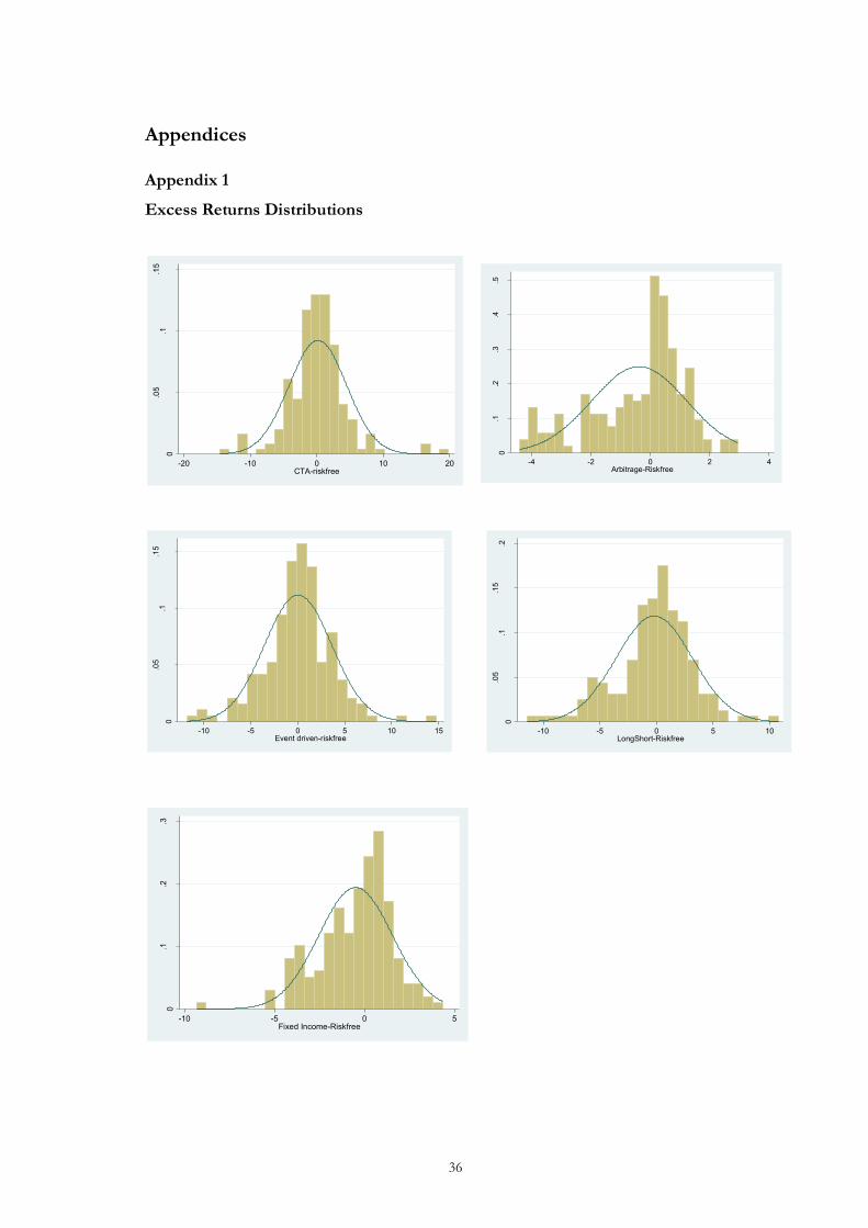
36
Appendices
Appendix 1
Excess Returns Distributions
0
.05
.1.1
5
Den
sity
-20 -10 0 10 20CTA-riskfree
0.1
.2.3
.4.5
Den
sity
-4 -2 0 2 4Arbitrage-Riskfree
0
.05
.1.1
5.2
Den
sity
-10 -5 0 5 10LongShort-Riskfree
0
.05
.1.1
5
Den
sity
-10 -5 0 5 10 15Event driven-riskfree
0.1
.2.3
Den
sity
-10 -5 0 5Fixed Income-Riskfree

37
Returns – Absolute values

38
Jan
2002
-Dec
200
5Ja
n 20
04-D
ec 2
007
Jan
2006
-Dec
200
9Ja
n 20
08-D
ec 2
011
Jan
2010
-Dec
201
3Ja
n 20
12-D
ec 2
015
Jan
2014
-Dec
201
6A
rbitr
age
Mea
n ex
cess
ret
urn
-0,5
7-2
,26
-1,6
50,
180,
350,
570,
64
Stan
dard
dev
iatio
n1,
201,
422,
001,
150,
800,
820,
88
Man
aged
fut
ures
Mea
n ex
cess
ret
urn
0,16
-3,0
6-1
,05
2,24
1,04
0,74
0,71
Stan
dard
dev
iatio
n4,
184,
386,
484,
302,
371,
882,
23
Eve
nt d
riven
Mea
n ex
cess
ret
urn
0,90
-1,2
0-1
,47
-0,2
20,
430,
580,
45
Stan
dard
dev
iatio
n4,
572,
843,
673,
712,
732,
502,
13
Lon
g/sh
ort
Mea
n ex
cess
ret
urn
0,17
-1,3
4-1
,39
-0,3
80,
330,
540,
25
Stan
dard
dev
iatio
n2,
942,
754,
454,
532,
742,
452,
58
Fixe
d In
com
eM
ean
exce
ss r
etur
n -0
,55
-2,3
7-1
,86
0,19
0,44
0,19
0,23
Stan
dard
dev
iatio
n1,
321,
612,
772,
391,
531,
331,
22
Mai
n he
dge
fund
inde
xJa
n 20
02-D
ec 2
016
Jan
2002
-Dec
200
5Ja
n 20
04-D
ec 2
007
Jan
2006
-Dec
200
9Ja
n 20
08-D
ec 2
011
Jan
2010
-Dec
201
3Ja
n 20
12-D
ec 2
015
Jan
2014
-Dec
201
6M
ean
(%)
-0,5
134
-0,7
104
-2,3
156
-1,8
399
0,02
050,
4666
0,43
390,
2111
Stan
dard
Err
or (%
)0,
1449
0,20
560,
2564
0,37
990,
3117
0,18
470,
1367
0,14
58St
anda
rd D
evia
tion
(%)
1,94
341,
4241
1,77
612,
6323
2,15
971,
2799
0,94
700,
8749
Min
imum
(%)
-5,9
827
-4,4
420
-5,9
827
-5,9
827
-5,2
985
-2,5
395
-1,9
336
-1,9
686
Max
imum
(%)
4,89
862,
7151
1,10
264,
8986
4,89
863,
0204
2,24
931,
6413
S&P
500
Jan
2002
-Dec
201
6Ja
n 20
02-D
ec 2
005
Jan
2004
-Dec
200
7Ja
n 20
06-D
ec 2
009
Jan
2008
-Dec
201
1Ja
n 20
10-D
ec 2
013
Jan
2012
-Dec
201
5Ja
n 20
14-D
ec 2
016
Mea
n (%
)-0
,721
1-1
,446
2-2
,682
9-2
,686
5-0
,522
21,
0715
1,01
680,
4760
Stan
dard
Err
or (%
)0,
3337
0,58
200,
3606
0,76
050,
8849
0,58
450,
4368
0,51
28St
anda
rd D
evia
tion
(%)
4,47
684,
0319
2,49
855,
2692
6,13
094,
0493
3,02
603,
0768
Min
imum
(%)
-17,
2025
-12,
6524
-8,0
343
-17,
2025
-17,
2025
-8,3
476
-6,3
351
-6,2
881
Max
imum
(%)
10,7
623
7,04
491,
9795
9,30
2510
,762
310
,762
38,
2883
8,28
83
Risk
-adj
uste
d re
turn
for s
ub-p
erio
ds

39
Appendix 2 Further explanations
Standard deviation
Standard deviation, or volatility is a measure of risk of a probability distribution. Or in other
words, a measure of how much an asset's return varies from its mean return. The standard
deviation is calculated by taking the square root of the variance, the assets expected squared
deviation from its mean.
𝑆𝐷 = 𝑉𝑎𝑟(𝑅𝑖𝑡) It's a positive relationship between return and volatility, so there is a tradeoff between risk
and return, the underlying assumption is that higher expected return results in higher risk,
or volatility (Berk & DeMarzo, 2014).
Moving average
To get a more relevant and reliable measures we have chosen to use the method of “Moving
Average” (sometimes called Moving Windows). The purpose of the method is to track
trends, by smoothing out the fluctuations. One of the most used type of moving averages
and the one method that we are using in this paper is, the Simple Moving Average (SMA).
The SMA is calculated by computing the average returns (or average prices if you want to
calculate a stock price) over a set of days, week or months. As the term implies, moving
averages is averages that moves on the timeline. Along our timeline of 180 months, from
January 2002 to December 2016, we use moving averages of 48 months (observations) that
overlap 24 months each time to get a total of seven “sub-averages” with the last containing
36 months. In that way, instead of getting one alpha-value for the whole observation period,
we can see how the alpha have moved during different stages of the observation period, such
as the last financial crisis (Law, 2009; Upton, 2011).
Risk - Systematic risk and unsystematic risk
Risk in the financial market are usually divided into systematic risk and asymmetric risk,
where they sum up to the total risk. Systematic risk (undiversifiable risk), is due to market-
wide news that result in fluctuations of a security's return. Risk that affect the overall market
and not only a specific security or stock. Systematic risk cannot be eliminated through
diversification. Systematic risk is impossible to avoid and hard to predict. Unsystematic risk

40
on the other hand, is inherited in different industries and companies and can therefore be
diversified by investing in stock from different industries (Hamberg, 2001; Berk & DeMarzo,
2014).
According to Markowitz (1952), a portion of volatility in the portfolio can be reduced by
combining different assets that don’t correlate with each other, by diversification. Hedge
funds (and mutual funds) reduce their unsystematic risk by investing in assets from various
industries. Hence, since diversification eliminates the unsystematic risk, investors are more
interested in how to measure and understand the systematic risk (Ross, Westerfield, Jaffe, &
Jordan, 2008).
Market proxy
The market proxy, can be explained as a measurement for comparing different funds to the
overall market or industry. In other words, a benchmark is selected so that one can compare
different funds’ performance in relation to a set of related various assets. A good benchmark
needs to fulfil some requirements; the securities in the benchmark needs to be clearly defined
where one should be able to see its weight. It also needs to be accessible, that is, a security
can be purchased on the market and the return should be able to be calculated often, and it
needs to have available past data. The CAPM suggest that the market proxy should be the
market portfolio. However, a market portfolio for all the risky securities in the world is hard
to find, whereas the S&P 500 is a commonly used and accepted market proxy since it explains
the overall health of the US economy. Since hedge funds are a special case and are placed
under the category of special funds and place its assets using different strategies in different
countries and industries it is hard to find an appropriate benchmark that can be applied to
all hedge funds. There is really no “one size fits all” benchmark. Based on the above
assumptions, the Eurekahedge main index consisting of 2797 funds is a representative hedge
fund performance market proxy because of its ability to explain the hedge fund industries
current state of mind (Fung & Hsieh, 2004; Berk & DeMarzo, 2014).