the phantom decoy effect in perceptual decision · pdf filethe phantom decoy effect in...

The Phantom Decoy Effect in Perceptual Decision-making

1

RUNNING HEAD: The Phantom Decoy Effect in Perceptual Decision-making


Jennifer S. Trueblood

Vanderbilt University and University of California, Irvine

Jonathan C. Pettibone

Southern Illinois University Edwardsville

Jennifer Trueblood Department of Psychology Vanderbilt University PMB 407817 2301 Vanderbilt Place Nashville, TN 37240-7817 phone: 615-343-7554 email: [email protected]


2

Abstract

A phantom decoy is an alternative that is superior to another “target” option, but is

unavailable at the time of choice. In value-based decisions involving phantom decoys (e.g.,

consumer choices), individuals often show increased preference for the similar, inferior target

option over a non-dominated competitor alternative. Unlike value-based decisions that are driven

by subjective goals, perceptual decisions typically have an outside criterion that defines the goal

of the task (e.g., target is present or absent). Despite their obvious differences, past research has

documented a number of commonalities between both types of decisions. In a set of three

experiments, we examine the influence of phantom options on simple perceptual decisions and

point out a critical difference between perceptual and value-based decisions. Our results show

that in perceptual choice, participants prefer competitor options to target options, the opposite of

the pattern typically found in consumer choice. We use the results of the experiments to examine

the predictions of four different models of context effects including loss aversion and dynamic,

preference accumulation models. We find that accumulation models provide the best explanation

for our results as well as being able to generalize to other context effects.

Keywords: phantom decoy, context effects, multi-alternative choice, perceptual decision-making

Word count: 8,944


3

THE PHANTOM DECOY EFFECT IN PERCEPTUAL DECISION-MAKING

When presented with multiple alternatives, preference has been shown to depend both

upon the values of the attributes of the alternatives themselves and upon the comparisons made

between them. These comparisons make up the context of a particular choice set, and a large

volume of previous research has shown that changes in the context of a choice set can influence

preference. For example, consider a situation were you are deciding among three dishes at a

conference dinner. Your options are lobster, tilapia, or vegetable lasagna. You immediately

decide that the lobster sounds the best. However, when the waiter comes to take your order, he

announces that the lobster is sold out for the night. You then decide to go with the tilapia over

the vegetable lasagna. Now consider a slightly different version of the same problem. In this

scenario, your dinner options are tilapia, vegetable lasagna, and spaghetti with meatballs. You

immediately prefer the spaghetti with meatballs, but find out later that it is unavailable. In this

situation, you choose the vegetable lasagna over the tilapia. This simple example illustrates that

preferences between two options (tilapia and vegetable lasagna) are dependent on a third

unavailable option. This phenomenon is known as the phantom decoy effect (Pratkanis &

Farquhar, 1992; Pettibone & Wedell, 2000; Pettibone & Wedell, 2007).

Beside the phantom decoy, other types of decoys have been studied including the

asymmetrically dominated (AD) decoy (Huber, Payne, & Puto, 1982) and the compromise

(COM) decoy (Simonson, 1989), both of which differ upon the type of contextual comparisons

they provide as well as upon their availability to be chosen. In most cases, these decoys have

been shown to increase preference for a “target” alternative that has similar attributes to the

decoy (e.g., spaghetti with meatballs increases preference for vegetable lasagna). These effects

have largely been shown to be robust (see Frederick, Lee, and Baskin (2014) for some


4

exceptions) and have been useful in generating multiple models for explaining the contextual

sensitivity of preference. In an experiment using typical consumer products as alternatives,

Pettibone & Wedell (2000) demonstrated that participants preferred the alternative that was

targeted by phantom decoy 57% of the time, compared to only 43% of the time when it was not

targeted. Both COM and AD decoys have shown similar effect sizes in consumer choice, with

the exception that participants tend to choose an available compromise decoy more often than

other types of available decoys.

Decoy effects have typically been studied in value-based decision-making (i.e., choices

made on the basis of a decision-maker’s subjective goals), using stimuli such as consumer

products (Wedell & Pettibone, 1996) and job candidates (Highhouse, 1996). In contrast to value-

based decisions, perceptual decisions require individuals to determine an unknown state of the

world (e.g., target present or absent) using noisy sensory information (Gold & Shadlen, 2007).

Like value-based decisions, people make perceptual decisions everyday. These decisions are

typically made quickly without much deliberation, for example, deciding if a traffic light is red

or green. Even though there is a clear difference between perceptual and value-based decisions,

the two types of decisions both require individuals to process uncertain information before a

choice can be made. Some researchers (Busemeyer, Jessup, Johnson, & Townsend, 2006;

Shadlen, Kiani, Hanks, & Churchland, 2008; Summerfield & Tsetsos, 2012; Symmonds &

Dolan, 2012) have even suggested that both types of decisions involve the same underlying

mechanisms.

Recently, researchers have shown that asymmetric dominance and compromise effects

occur in perceptual choice tasks as well as value-based decisions (Choplin & Hummel, 2005;

Trueblood, Brown, Heathcote, & Busemeyer, 2013), suggesting that the processes that lead to


5

decoy effects may involve fundamental processes (at a low cognitive level) rather than higher-

level heuristics. Phantom decoy effects, however, have not been demonstrated in perceptual

choice. The phantom decoy, unlike other decoys (i.e., AD and COM decoys), is a superior but

unavailable option that typically results in increased preference for a similar target alternative

that it dominates (Pettibone & Wedell, 2007). This paper examines the influence of phantom

decoys in perceptual decisions and points out a crucial difference between these decisions and

value-based ones. We also use the results of our experiments to test the predictions of four

different models of phantom decoy effects.

Overview of Decoy Effects

In order to understand the phantom decoy, we first explain decoy effects in general and

the asymmetric dominance and compromise effects in specific. Decoy effects typically

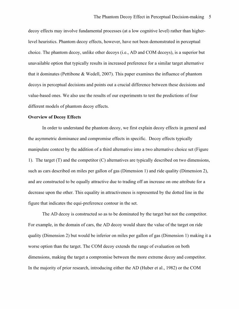
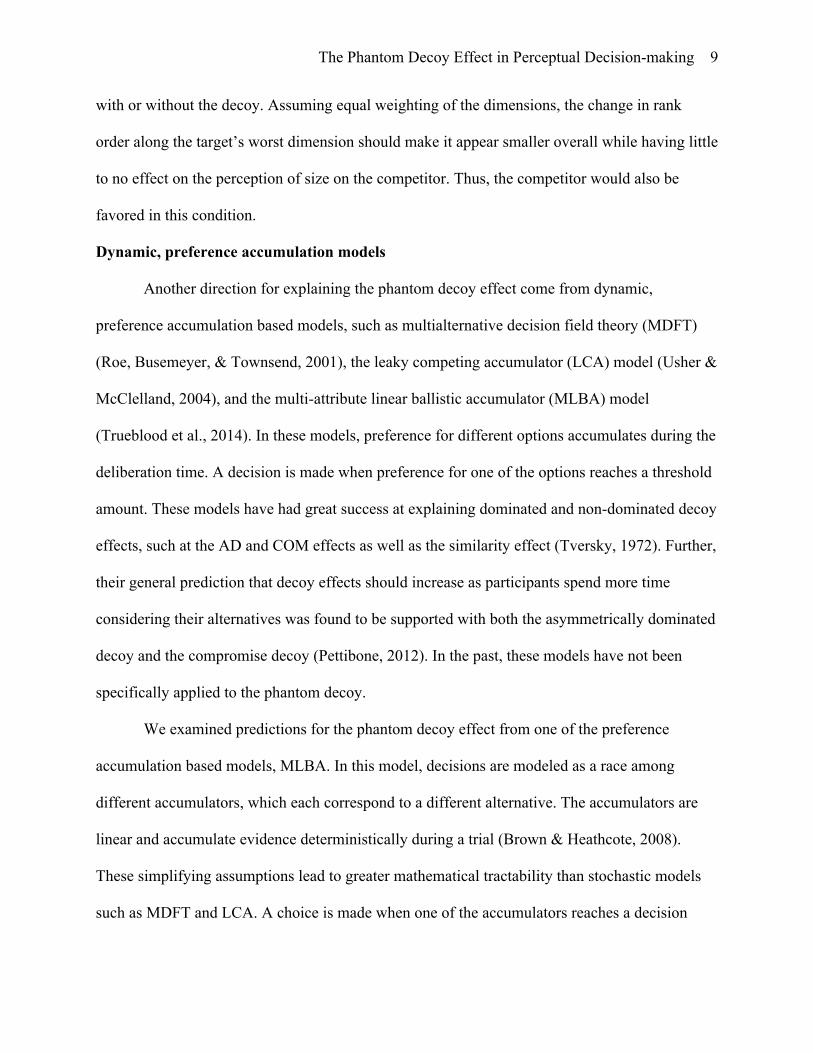
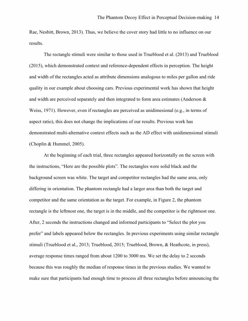
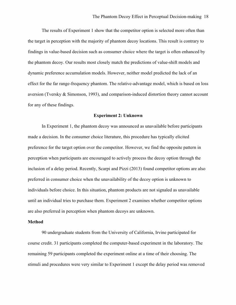
manipulate context by the addition of a third alternative into a two alternative choice set (Figure

1). The target (T) and the competitor (C) alternatives are typically described on two dimensions,

such as cars described on miles per gallon of gas (Dimension 1) and ride quality (Dimension 2),

and are constructed to be equally attractive due to trading off an increase on one attribute for a

decrease upon the other. This equality in attractiveness is represented by the dotted line in the

figure that indicates the equi-preference contour in the set.

The AD decoy is constructed so as to be dominated by the target but not the competitor.

For example, in the domain of cars, the AD decoy would share the value of the target on ride

quality (Dimension 2) but would be inferior on miles per gallon of gas (Dimension 1) making it a

worse option than the target. The COM decoy extends the range of evaluation on both

dimensions, making the target a compromise between the more extreme decoy and competitor.

In the majority of prior research, introducing either the AD (Huber et al., 1982) or the COM


6

(Simonson, 1989) decoys into the choice set increases preference for the target and decreases

preference for the competitor, violating rational choice theory and creating the potential for

preference reversals by flipping the locations of the decoys to favor the competitor.

Phantom Decoy

In comparison, phantom decoys are constructed to dominate the target, but are presented

to participants as unavailable. In the case of the car example, a range phantom decoy (PR) would

have the same value on miles per gallon of gas as the target (Dimension 1) but would be superior

on ride quality (Dimension 2). In comparison to the competitor, this phantom would be superior

overall but would have a lower value on miles per gallon of gas. The phantom decoy, then,

simulates a situation where a highly attractive but unavailable alternative is present in the

marketplace. In these cases, participants also prefer the target (Pratkinis & Farquar, 1992;

Highhouse, 1996; Pettibone & Wedell, 2000, 2007) despite the fact that the decoy dominates it.

Across a number of studies, the types of phantoms that have previously been tested vary

depending upon two factors: location relative to the target and awareness of its unavailability.

Past studies (Pettibone & Wedell, 2007; Scarpi & Pizzi, 2013), have used phantom decoys at

different locations to examine how decoy placement influences the strength of the effect. In our

experiments, we include five different decoy locations as shown in Figure 1.

For the phantom decoy to have an influence on preference, participants must compare it

to the available alternatives in the set. Most prior research with consumer stimuli has attempted

to hide the unavailability of the phantom in some way to make sure that participants consider it.

The exact method of making participants aware of the unavailability of the phantom, however,

may have an impact on the effect seen. In the majority of studies on phantom decoys,

participants are presented the three alternatives in the set simultaneously without being aware


7

that the decoy is unavailable. After a brief delay, 3 seconds in studies by Pettibone & Wedell

(2000, 2007), but before a choice is made, participants are told that the phantom is unavailable

and that they need to make their choice from the remaining items (we call this a known delay

presentation). A second method, which we call unknown presentation, hides the unavailability of

the phantom until after participants make a choice. If a participant chooses the phantom, only

then are they told of its unavailability and are required to make a different choice. Scarpi and

Pizzi (2013) found that this type of presentation resulted in preference for the competitor over

the target for certain decoy locations. They argued that not knowing the phantom was

unavailable in advance triggered a negative affective reaction due to the unexpected loss of

choice freedom, decreasing the overall attractiveness of the target. Specifically, they showed

that judgments of justice, decision satisfaction, and intent to repatronize after a decision all

declined when compared to choice sets containing a known phantom. A third approach is to

simply mark the phantom as unavailable from stimulus onset.

Models of the Phantom Decoy Effect

Finding a theoretical explanation of the phantom decoy effect, especially one that can

simultaneously explain other types of decoys, has been difficult. Typically, models used to

explain AD and COM effects have struggled to explain why participants choose the dominated

target with the phantom decoy. In this section, we briefly review four different models of AD

and COM effects and discuss their predictions regarding the phantom decoy.

Value-shift models

Value-shift models (Wedell & Pettibone, 1999) rely upon changes in the subjective

valuation of attributes due to context, such as predicted by range-frequency theory (Parducci,

1974). In the case of the AD decoy, the extension of range on the target’s worst attribute


8

increases its subjective valuation, causing it to increase in overall value. The same extension of

range does little to help the competitor, since it is already superior on that attribute. This model,

however, does not predict COM. In this case, range is extended on both attributes, which should

result in no increase in preference for the target since both extensions should cancel each other

out (Pettibone & Wedell, 2000).

In the case of phantom decoys, other than the frequency phantom (PF in Figure 1), the

extension of range on the target’s best attribute should actually make the target appear less

attractive, and would favor the selection of the competitor. For example, in a two-item choice

set, the target is the best on one attribute. Adding the range or the extended range phantom decoy

(PR and PER in Figure 1) extends the range on the best attribute of the target, pushing the target

into the middle of the pack. In comparison, the competitor suffers relatively little loss of value

because it already had the lowest value on that attribute. Indeed, this is what Pettibone and

Wedell (2000) found when they looked at attribute value ratings individually for each alternative

with the phantom decoy. Despite this shift, participants still preferred the target in choice,

suggesting that while these processes still operate, they do not govern preference with the

phantom decoy in consumer choice. However, in perceptual choice, these processes may still

operate. If this is true, participants should choose the competitor as the largest shape in all

awareness of unavailability conditions except for the known condition.

As for the frequency phantom, while there is no extension of range due to its

presentation, the rankings of the three alternatives do change along the target’s worst dimension.

This makes the target move from being the second smallest on that dimension to the third. The

presentation of the frequency phantom does not change the rank order along the target’s best

dimension as it shares that value with the target, leaving the competitor as the second smallest


9

with or without the decoy. Assuming equal weighting of the dimensions, the change in rank

order along the target’s worst dimension should make it appear smaller overall while having little

to no effect on the perception of size on the competitor. Thus, the competitor would also be

favored in this condition.

Dynamic, preference accumulation models

Another direction for explaining the phantom decoy effect come from dynamic,

preference accumulation based models, such as multialternative decision field theory (MDFT)

(Roe, Busemeyer, & Townsend, 2001), the leaky competing accumulator (LCA) model (Usher &

McClelland, 2004), and the multi-attribute linear ballistic accumulator (MLBA) model

(Trueblood et al., 2014). In these models, preference for different options accumulates during the

deliberation time. A decision is made when preference for one of the options reaches a threshold

amount. These models have had great success at explaining dominated and non-dominated decoy

effects, such at the AD and COM effects as well as the similarity effect (Tversky, 1972). Further,

their general prediction that decoy effects should increase as participants spend more time

considering their alternatives was found to be supported with both the asymmetrically dominated

decoy and the compromise decoy (Pettibone, 2012). In the past, these models have not been

specifically applied to the phantom decoy.

We examined predictions for the phantom decoy effect from one of the preference

accumulation based models, MLBA. In this model, decisions are modeled as a race among

different accumulators, which each correspond to a different alternative. The accumulators are

linear and accumulate evidence deterministically during a trial (Brown & Heathcote, 2008).

These simplifying assumptions lead to greater mathematical tractability than stochastic models

such as MDFT and LCA. A choice is made when one of the accumulators reaches a decision


10

threshold. The rate of evidence accumulation for a particular alternative is determined by

comparing the alternative to each of the other items in the choice set. Specifically, comparisons

are performed along each attribute where favorable comparisons (those where the alternative has

a better attribute value) result in positive evaluations and unfavorable comparisons result in

negative evaluations. All of the evaluations for a particular alternative are combined into a single

value (the drift rate) that specifics how quickly the accumulator for that alternative will race. For

more details, please see Appendix B.

MLBA predicts that individuals will prefer the competitor to the target for all phantom

decoy locations as illustrated in Figure 1. In the model, there are more favorable comparisons

between the competitor and phantom than the target and phantom because the competitor is

superior to the phantom on one dimension. Essentially, the model is capturing the fact that the

target and phantom are easy to compare (i.e., the options have similar attribute values) whereas

the competitor and phantom are more difficult to compare (i.e., the options have dissimilar

attribute values). This ultimately leads to a larger drift rate for the competitor as compared to the

target. The shades in the figure show the relative choice share of the target (RST), which is the

number of times the target was selected divided by the number of times the target plus

competitor was selected (Berkowitsch, Scheibehenne, & Rieskamp, 2014; Trueblood, 2015).

RST values with light shades indicate values greater than .5 (i.e., preference for the target) and

dark shades indicate values less than .5 (i.e., preference for the competitor) Simulation details are

also provided in Appendix B. Similar to value shift models, MLBA predicts the competitor as

the largest shape in all awareness of unavailability conditions except for the known condition.

Loss Aversion


11

Another proposed explanation for decoy effects, including the phantom decoy effect, is

based on the relative-advantage model which works on the principle of loss-aversion (Tversky &

Simonson, 1993). In multi-alternative, multi-attribute choice, loss aversion is characterized by

the asymmetric weighting of positive and negative differences between the attributes of options.

The relative-advantage model predicts that after setting the phantom as the reference point,

participants are motivated to select the alternative (i.e. the target) that represents the least loss

from it.

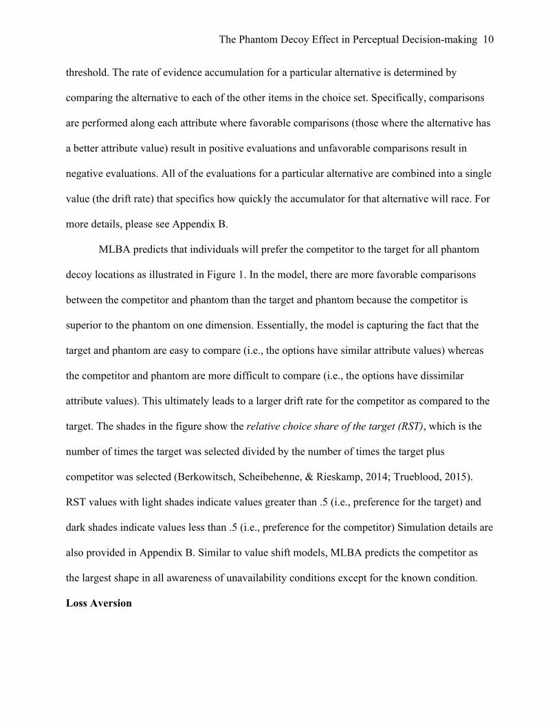
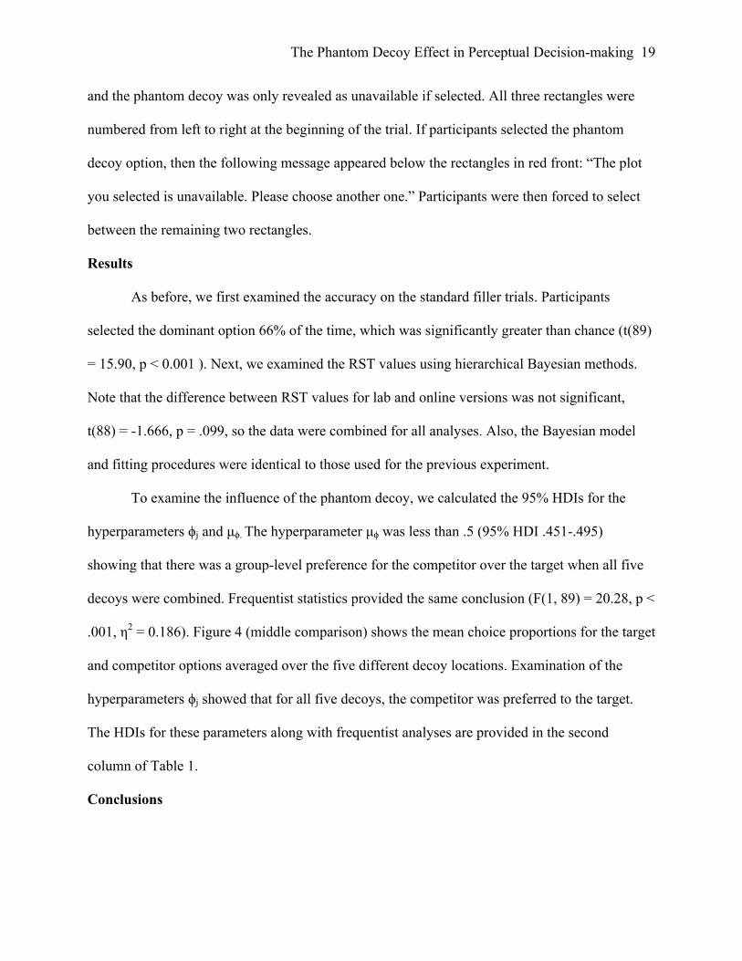
Perceptual choice tasks provide an opportunity to test the loss aversion hypothesis. In our

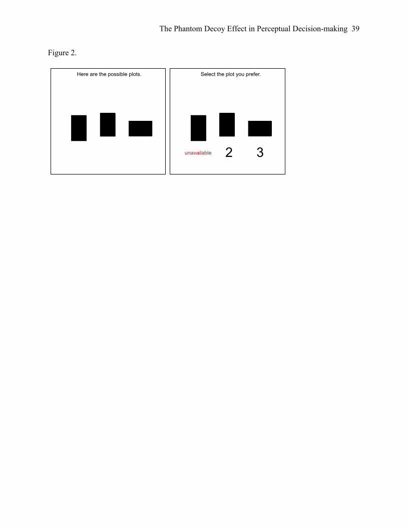
task, participants are shown sets of three rectangles and are told to choose the largest one (see

Figure 2 for an example). Loss aversion would imply that people weight a “loss” in height

(width) between two rectangles more than an equivalent “gain” in width (height) between the

same two rectangles. We argue that such an asymmetrical weighting does not make sense in our

task. Thus, it is difficult to imagine a loss-aversion based process operating in a simple size

judgment task, as participants have no potential loss other than the possibility of being wrong.

Note that loss aversion is different from error aversion where people experience greater neural

feedback from errors than correct responses. If phantom decoy effects were truly due to loss

aversion, then one would expect to find no context effects in perceptual choice where loss

aversion does not operate. More specifically, the relative-advantage model, which is based on

loss-aversion, predicts no context effects if the loss aversion parameter is equal to one (i.e., no

loss aversion).

Comparison-induced distortion theory

Another model that may account for AD, COM, and Phantom decoy effects, but has not

been tested with all three, is Choplin and Hummel’s Comparison-Induced distortion Theory


12

(2002). They argue that the type of comparison that is made between alternatives depends upon

the goal of the decision maker. If they are trying to find the best option, as is the case with the

AD and COM decoys, participants will make comparisons that emphasize differences between

the options, leading to distortions in perception that favor the target. In the case of the phantom,

however, the decoy is the best option, which changes the goal of the task from finding

differences with the decoy to finding similarity to the decoy. Searching for the option that is

most similar to the decoy would lead to the choice of the target.

Experiment Overview

In our experiments we test the qualitative predictions of the four models described above.

Both value-shift models and dynamic preference accumulation models predict that the phantom

decoy will increase preference for the competitor over the target. The relative-advantage model

(when the loss aversion parameter is greater than one) and comparison-induced distortion theory

predict the opposite pattern – increased preference for the target over the competitor, In our task,

we present participants with a series of choice sets containing three rectangles of varying sizes.

Participants are asked to choose the shape that they feel is the largest (see Figure 2 for an

example). The rectangles vary based on their height and width, with these dimensions serving the

role of attributes in consumer choice. The target and competitor rectangles have the exact same

area, but differ in their lengths along the two dimensions (i.e., they have different orientations).

The phantom decoy (left rectangle in Figure 2) has a larger area than both the target and

competitor rectangles and the same orientation as the target. Across all experiments, we tested

the five phantom decoy locations as shown in Figure 1: range, extended range, frequency, near

range-frequency, and far range-frequency. In Experiment 1, we tested them when informing

participants of the unavailability of the phantom after a short delay (known with delay). In


13

Experiment 2, we only told participants of the unavailability of the decoy after they made their

initial choice (unknown). Finally, in Experiment 3, we told participants of the unavailability of

the decoy from stimulus onset (known without delay).

Experiment 1: Known with delay

In the first experiment, the phantom is known prior to choice; however, there is a delay

between the initial presentation of the alternatives and announcement of the unavailable

phantom. On each trial, participants view three rectangles and are instructed to choose the one

with the largest area. Phantom options are clearly larger than the remaining two rectangles.

Method

84 undergraduate students from the University of California, Irvine participated for

course credit. 31 participants completed the computer-based experiment in the laboratory. The

remaining 53 participants completed the experiment online at a time of their choosing.

Participants read the following cover story and instructions: “In this task you will imagine that

you are a farmer who leases plots of land for growing crops. The plots of land will be shown to

you as black rectangles. Your job is to choose the plot of land (i.e., rectangle) that you think as

the largest area in order to maximize your growing space. At the beginning of each trial, you will

be shown tree possible plots of land. Then, you will be asked to select the one you prefer.”

Participants were also told that on some trials one of the rectangles might be labeled as

unavailable. In this situation, they were instructed to choose between the two remaining

rectangles. In previous experiments using similar rectangle stimuli, no differences were found

between experiments using the farmland cover story and those without a cover story (Trueblood,

2015). Further, researchers have shown that incorporating gamelike features into standard

experimental tasks, while leaving the basic task unchanged, does not alter behavior (Hawkins,


14

Rae, Nesbitt, Brown, 2013). Thus, we believe the cover story had little to no influence on our

results.

The rectangle stimuli were similar to those used in Trueblood et al. (2013) and Trueblood

(2015), which demonstrated context and reference-dependent effects in perception. The height

and width of the rectangles acted as attribute dimensions analogous to miles per gallon and ride

quality in our example about choosing cars. Previous experimental work has shown that height

and width are perceived separately and then integrated to form area estimates (Anderson &

Weiss, 1971). However, even if rectangles are perceived as unidimesional (e.g., in terms of

aspect ratio), this does not change the implications of our results. Previous work has

demonstrated multi-alternative context effects such as the AD effect with unidimensional stimuli

(Choplin & Hummel, 2005).

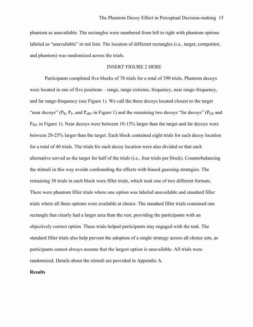
At the beginning of each trial, three rectangles appeared horizontally on the screen with

the instructions, “Here are the possible plots”. The rectangles were solid black and the

background screen was white. The target and competitor rectangles had the same area, only

differing in orientation. The phantom rectangle had a larger area than both the target and

competitor and the same orientation as the target. For example, in Figure 2, the phantom

rectangle is the leftmost one, the target is in the middle, and the competitor is the rightmost one.

After, 2 seconds the instructions changed and informed participants to “Select the plot you

prefer” and labels appeared below the rectangles. In previous experiments using similar rectangle

stimuli (Trueblood et al., 2013; Trueblood, 2015; Trueblood, Brown, & Heathcote, in press),

average response times ranged from about 1200 to 3000 ms. We set the delay to 2 seconds

because this was roughly the median of response times in the previous studies. We wanted to

make sure that participants had enough time to process all three rectangles before announcing the


15

phantom as unavailable. The rectangles were numbered from left to right with phantom options

labeled as “unavailable” in red font. The location of different rectangles (i.e., target, competitor,

and phantom) was randomized across the trials.

INSERT FIGURE 2 HERE

Participants completed five blocks of 78 trials for a total of 390 trials. Phantom decoys

were located in one of five positions – range, range extreme, frequency, near range-frequency,

and far range-frequency (see Figure 1). We call the three decoys located closest to the target

“near decoys” (PR, PF, and PnRF in Figure 1) and the remaining two decoys “far decoys” (PER and

PfRF in Figure 1). Near decoys were between 10-15% larger than the target and far decoys were

between 20-25% larger than the target. Each block contained eight trials for each decoy location

for a total of 40 trials. The trials for each decoy location were also divided so that each

alternative served as the target for half of the trials (i.e., four trials per block). Counterbalancing

the stimuli in this way avoids confounding the effects with biased guessing strategies. The

remaining 38 trials in each block were filler trials, which took one of two different formats.

There were phantom filler trials where one option was labeled unavailable and standard filler

trials where all three options were available at choice. The standard filler trials contained one

rectangle that clearly had a larger area than the rest, providing the participants with an

objectively correct option. These trials helped participants stay engaged with the task. The

standard filler trials also help prevent the adoption of a single strategy across all choice sets, as

participants cannot always assume that the largest option is unavailable. All trials were

randomized. Details about the stimuli are provided in Appendix A.

Results


16

We first examined the accuracy on the standard filler trials. Participants selected the

dominant option 80% of the time, which was significantly greater than the guessing rate of 33%

(t(83) = 26.50, p < 0.001). Because participants preferred the dominant option on the filler trials,

we have good reason to believe that they also preferred the phantom on test trials. Next, we

evaluated the influence of the phantom decoys using the RST value. If the RST is greater than .5,

then the target is selected more often than the competitor. If the RST value is less than .5, then

the competitor is preferred to the target. RST values equal to .5 imply the target and competitor

are selected equally often showing an absence of any influence of the phantom decoy. The

difference between RST values for lab and online versions of the experiment was not significant,

t(82) = -0.034, p = .973, so the data were combined for all analyses. Following recent methods

for analyzing context effects (Berkowitsch, Scheibehenne, & Rieskamp, 2014; Trueblood, 2015;

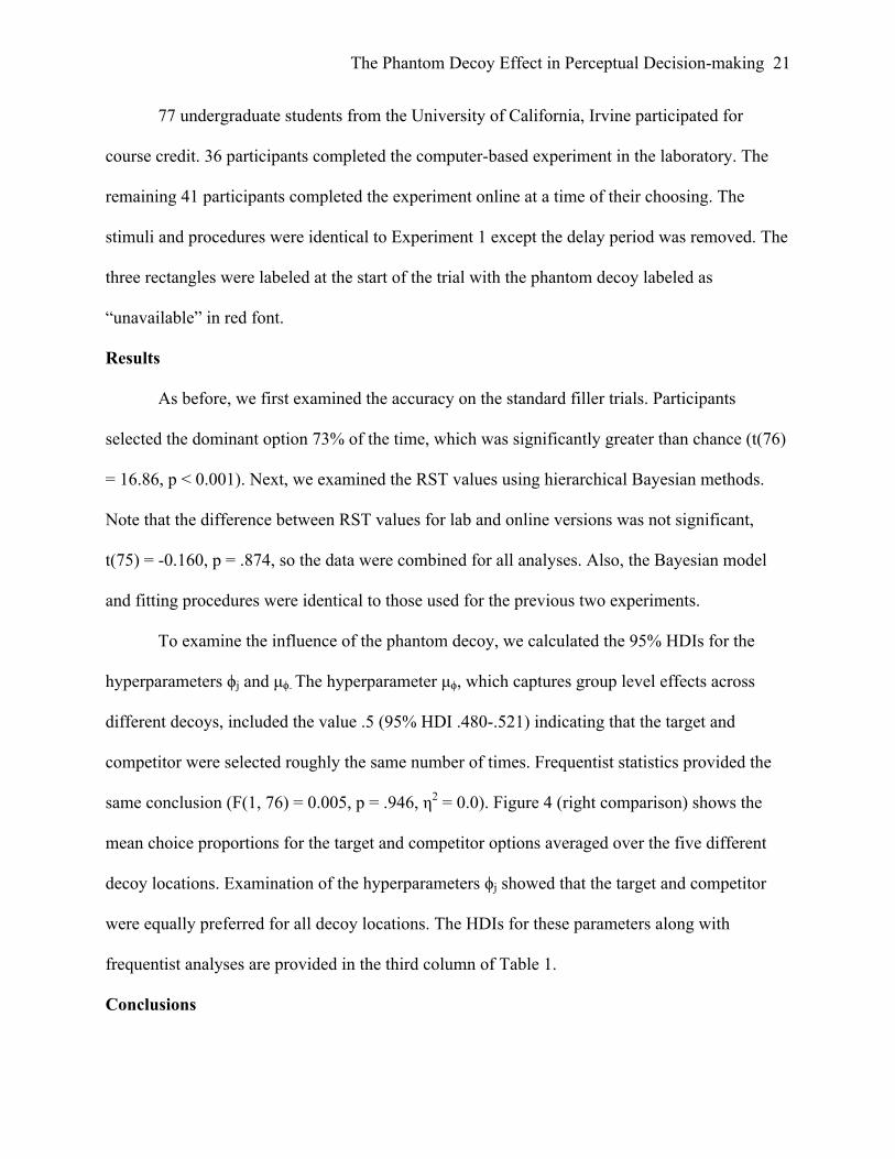
Trueblood, Brown, & Heathcote, in press), we used a hierarchical Bayesian model to test

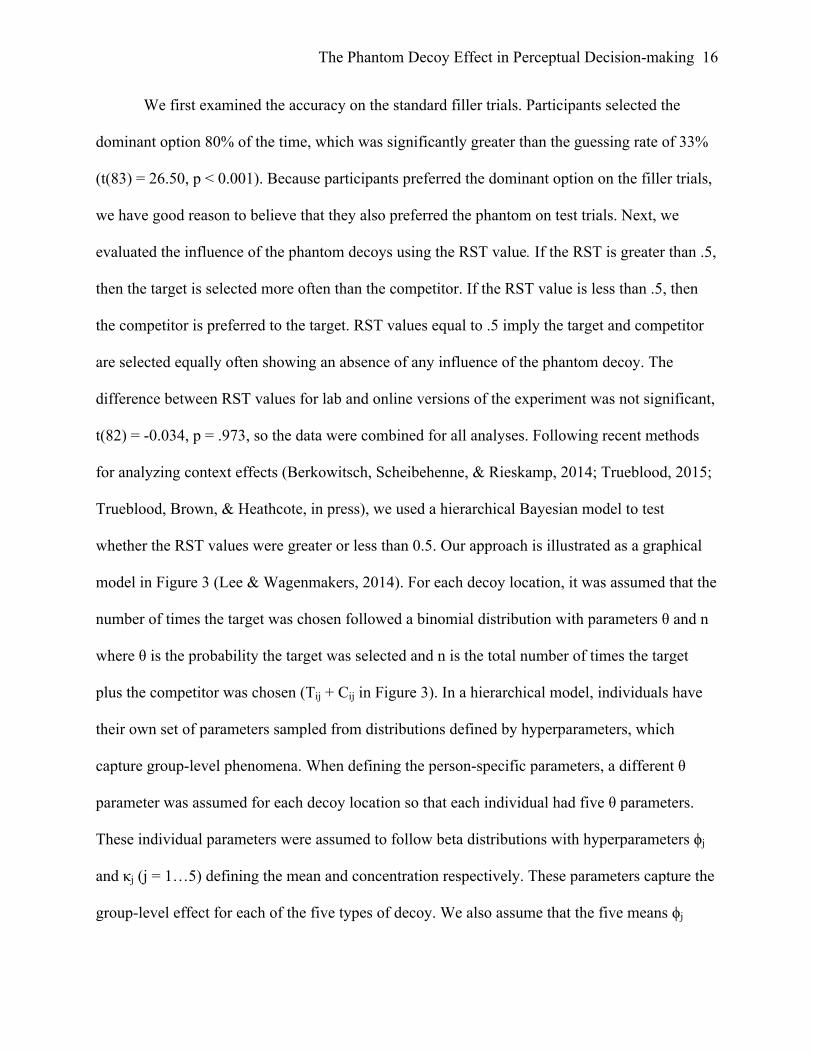
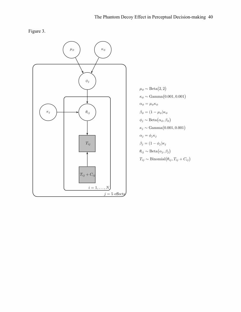
whether the RST values were greater or less than 0.5. Our approach is illustrated as a graphical

model in Figure 3 (Lee & Wagenmakers, 2014). For each decoy location, it was assumed that the

number of times the target was chosen followed a binomial distribution with parameters θ and n

where θ is the probability the target was selected and n is the total number of times the target

plus the competitor was chosen (Tij + Cij in Figure 3). In a hierarchical model, individuals have

their own set of parameters sampled from distributions defined by hyperparameters, which

capture group-level phenomena. When defining the person-specific parameters, a different θ

parameter was assumed for each decoy location so that each individual had five θ parameters.

These individual parameters were assumed to follow beta distributions with hyperparameters ϕj

and κj (j = 1…5) defining the mean and concentration respectively. These parameters capture the

group-level effect for each of the five types of decoy. We also assume that the five means ϕj


17

follow a beta distribution with parameters µϕ and κϕ, which capture the group-level effect across

all five decoys combined.1 Three MCMC chains were used to estimate the posterior distributions

for the parameters (both person-specific and hierarchal) using JAGS.2


The 95% highest posterior density intervals (HDIs) for the hyperparameters ϕj and µϕ

represent the most credible posterior RST values from the Bayesian analysis for individual

decoys and combined decoys, respectively (Kruschke, 2010). If this region lies above .5, then

one can infer that the target was preferred to the competitor. Likewise, if this region lies below

.5, then the competitor was preferred to the target. The hyperparameter µϕ was less than .5 (95%

HDI .453-.499) showing that there was a group-level preference for the competitor over the

target when all five decoys were combined. Frequentist statistics provided the same conclusion

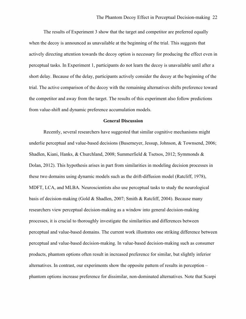
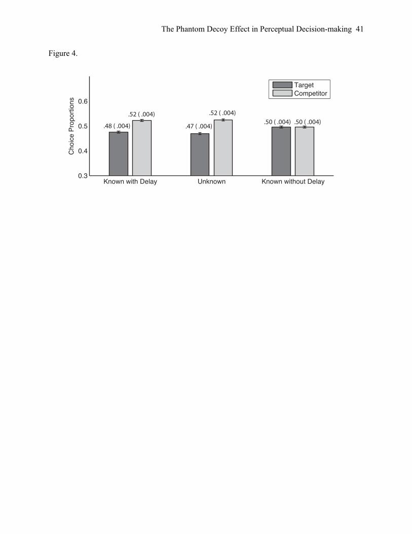
(F(1,83) = 25.10, p < .001, η2 = 0.232). Figure 4 (left comparison) shows the mean choice

proportions for the target and competitor options averaged over the five different decoy

locations. Examination of the hyperparameters ϕj showed that for four out of five decoys (all but

the far range-frequency decoy), the competitor was preferred to the target. The HDI values for

these parameters along with frequentist analyses are provided in the first column of Table 1.


INSERT TABLE 1 HERE

Conclusions

1 The prior for µϕ was a beta distribution with both shape parameters equal to 2. This prior is considered vague and provides low certainty about the value of µϕ. It also slightly favors the null hypothesis that the RST across all decoys is equal to 0.5. The priors for κj and κϕ were gamma distributions with shape and rate parameters equal to 0.001. This is also a vague prior and is commonly used on precision parameters because it is invariant to changes in measurement scale (Lee & Wagenmakers, 2014). 2 Chain convergence was assessed by using the statistic, which is similar to the F statistic. Specifically, if is large, then the between-chain variance is larger than the within-chain variance. A value close to 1 is ideal and

values lower than 1.1 are considered satisfactory. All parameters had less than 1.1.

R̂ R̂R̂

R̂


18

The results of Experiment 1 show that the competitor option is selected more often than

the target in perception with the majority of phantom decoy locations. This result is contrary to

findings in value-based decision such as consumer choice where the target is often enhanced by

the phantom decoy. Our results most closely match the predictions of value-shift models and

dynamic preference accumulation models. However, neither model predicted the lack of an

effect for the far range-frequency phantom. The relative-advantage model, which is based on loss

aversion (Tversky & Simonson, 1993), and comparison-induced distortion theory cannot account

for any of these findings.

Experiment 2: Unknown

In Experiment 1, the phantom decoy was announced as unavailable before participants

made a decision. In the consumer choice literature, this procedure has typically elicited

preference for the target option over the competitor. However, we find the opposite pattern in

perception when participants are encouraged to actively process the decoy option through the

inclusion of a delay period. Recently, Scarpi and Pizzi (2013) found competitor options are also

preferred in consumer choice when the unavailability of the decoy option is unknown to

individuals before choice. In this situation, phantom products are not signaled as unavailable

until an individual tries to purchase them. Experiment 2 examines whether competitor options

are also preferred in perception when phantom decoys are unknown.

Method



remaining 59 participants completed the experiment online at a time of their choosing. The

stimuli and procedures were very similar to Experiment 1 except the delay period was removed


19

and the phantom decoy was only revealed as unavailable if selected. All three rectangles were

numbered from left to right at the beginning of the trial. If participants selected the phantom

decoy option, then the following message appeared below the rectangles in red front: “The plot

you selected is unavailable. Please choose another one.” Participants were then forced to select

between the remaining two rectangles.

Results

As before, we first examined the accuracy on the standard filler trials. Participants

selected the dominant option 66% of the time, which was significantly greater than chance (t(89)

= 15.90, p < 0.001 ). Next, we examined the RST values using hierarchical Bayesian methods.

Note that the difference between RST values for lab and online versions was not significant,

t(88) = -1.666, p = .099, so the data were combined for all analyses. Also, the Bayesian model

and fitting procedures were identical to those used for the previous experiment.

To examine the influence of the phantom decoy, we calculated the 95% HDIs for the

hyperparameters ϕj and µϕ. The hyperparameter µϕ was less than .5 (95% HDI .451-.495)

showing that there was a group-level preference for the competitor over the target when all five

decoys were combined. Frequentist statistics provided the same conclusion (F(1, 89) = 20.28, p <

.001, η2 = 0.186). Figure 4 (middle comparison) shows the mean choice proportions for the target

and competitor options averaged over the five different decoy locations. Examination of the

hyperparameters ϕj showed that for all five decoys, the competitor was preferred to the target.

The HDIs for these parameters along with frequentist analyses are provided in the second

column of Table 1.

Conclusions


20

The results of Experiment 2 show that the competitor option is selected more often than

the target when the phantom decoy is unknown. This finding is in agreement with the results of

Experiment 1 and results in consumer choice (Scarpi & Pizzi, 2013). In general, competitor

options are favored over target options in perception regardless of whether the phantom is known

(with a delay) or unknown to individuals. Further, all decoy locations increased preference for

the competitor. Similar to experiment 1, our results most closely match the predictions of both

dynamic preference accumulation and value-shift models.

Experiment 3: Known without Delay

In Experiment 1, the phantom decoy was announced as unavailable after a 2 second

delay. In the third experiment, we examined the necessity of this delay period by announcing the

decoy as unavailable at the beginning of the trial. In this way, the decoy is irrelevant to the task.

However, in many perceptual tasks, irrelevant information can have a substantial influence on

behavior. For example, in the Eriksen Flanker Task (Eriksen & Eriksen, 1974), participants make

decisions about targets, which are flanked by either congruent or incongruent noise stimuli.

Results show that participants cannot prevent processing the irrelevant information. In our task,

unintentional processing of the decoy option could influence behavior similarly to Experiment 1.

Alternatively, the decoy might only be effective if it is actively compared to the other options

during the trial. Recently, Noguchi and Stewart (2014) used eye tracking to show that visual

attention plays an important role in decoy effects in consumer choice. If active comparisons

between the decoy and other options are necessary for the effect, then we anticipate that the

decoy will have little to no effect when announced as unavailable at the beginning of the trial.

Method


21



remaining 41 participants completed the experiment online at a time of their choosing. The

stimuli and procedures were identical to Experiment 1 except the delay period was removed. The

three rectangles were labeled at the start of the trial with the phantom decoy labeled as

“unavailable” in red font.

Results

As before, we first examined the accuracy on the standard filler trials. Participants

selected the dominant option 73% of the time, which was significantly greater than chance (t(76)

= 16.86, p < 0.001). Next, we examined the RST values using hierarchical Bayesian methods.

Note that the difference between RST values for lab and online versions was not significant,

t(75) = -0.160, p = .874, so the data were combined for all analyses. Also, the Bayesian model

and fitting procedures were identical to those used for the previous two experiments.

To examine the influence of the phantom decoy, we calculated the 95% HDIs for the

hyperparameters ϕj and µϕ. The hyperparameter µϕ, which captures group level effects across

different decoys, included the value .5 (95% HDI .480-.521) indicating that the target and

competitor were selected roughly the same number of times. Frequentist statistics provided the

same conclusion (F(1, 76) = 0.005, p = .946, η2 = 0.0). Figure 4 (right comparison) shows the

mean choice proportions for the target and competitor options averaged over the five different

decoy locations. Examination of the hyperparameters ϕj showed that the target and competitor

were equally preferred for all decoy locations. The HDIs for these parameters along with

frequentist analyses are provided in the third column of Table 1.

Conclusions


22

The results of Experiment 3 show that the target and competitor are preferred equally

when the decoy is announced as unavailable at the beginning of the trial. This suggests that

actively directing attention towards the decoy option is necessary for producing the effect even in

perceptual tasks. In Experiment 1, participants do not learn the decoy is unavailable until after a

short delay. Because of the delay, participants actively consider the decoy at the beginning of the

trial. The active comparison of the decoy with the remaining alternatives shifts preference toward

the competitor and away from the target. The results of this experiment also follow predictions

from value-shift and dynamic preference accumulation models.

General Discussion

Recently, several researchers have suggested that similar cognitive mechanisms might

underlie perceptual and value-based decisions (Busemeyer, Jessup, Johnson, & Townsend, 2006;

Shadlen, Kiani, Hanks, & Churchland, 2008; Summerfield & Tsetsos, 2012; Symmonds &

Dolan, 2012). This hypothesis arises in part from similarities in modeling decision processes in

these two domains using dynamic models such as the drift-diffusion model (Ratcliff, 1978),

MDFT, LCA, and MLBA. Neuroscientists also use perceptual tasks to study the neurological

basis of decision-making (Gold & Shadlen, 2007; Smith & Ratcliff, 2004). Because many

researchers view perceptual decision-making as a window into general decision-making

processes, it is crucial to thoroughly investigate the similarities and differences between

perceptual and value-based domains. The current work illustrates one striking difference between

perceptual and value-based decision-making. In value-based decision-making such as consumer

products, phantom options often result in increased preference for similar, but slightly inferior

alternatives. In contrast, our experiments show the opposite pattern of results in perception –

phantom options increase preference for dissimilar, non-dominated alternatives. Note that Scarpi


23

and Pizzi (2013) also showed that phantom options increase preference for competitor

alternatives in consumer choice for both the range decoy (60.7% chose the competitor) and for

the extended range decoy (72% chose the competitor) in the unknown presentation mode.

Previous experiments using perceptual (Choplin & Hummel, 2005; Trueblood et al.,

2013; Trueblood, 2015) and psychophysical (Tsetsos, Chater, & Usher, 2012; Tsetsos, Usher, &

McClelland, 2011) stimuli have revealed similarities in choice behavior between low-level and

value-based decision tasks involving available decoys (e.g., AD and COM effects). These

experiments suggest that decoy effects are not solely the result of value-based phenomena such

as loss aversion (Tversky & Simonson, 1993). In perceptual tasks (e.g., decisions about the size

of rectangles), there is no notion of gains and losses. Rather, these experiments support the

hypothesis that decoy effects can also arise from fundamental processes.

In the present work, we illustrate a crucial difference between perceptual and value-based

decisions. This naturally leads to the question of what causes this difference. One possibility is

the influence of loss aversion in value-based decisions, which could reverse the direction of the

effect found in perceptual choice. Recently, Yechiam and Hochman (2013) found that losses can

enhance on-task attention, which might result in increased sensitivity to decoy effects in

consumer choice. In consumer choice tasks, loss aversion could override lower-order processes

resulting in preference for target alternatives when phantom decoys are present.

While loss aversion could modulate decoy effects in consumer choice, an important

question is determining the basic cognitive processes that produce these effects when losses are

not present. Based on the results of our experiments, range-frequency based value-shift processes

(Pettibone & Wedell, 2000) and dynamic preference accumulation models provide possible

explanations. However, value-shift models have limited explanatory power to capture a wide


24

range of context effects. They can only account for asymmetrically dominated decoy effects, but

not compromise effects and similarity effects as can dynamic preference accumulation models.

Accumulation models such as MLBA (Trueblood et al., 2014) can account for all three standard

context effects including the influence of time pressure on these effects. MLBA has also been

shown to provide good quantitative fits to choice data from several different tasks. It is one of

many dynamic models of multi-alternative, multi-attribute choice. Alternative dynamic models

include MDFT, LCA, the associative accumulation model (Bhatia, 2013), and the 2N-ary choice

tree (Wollschläger & Diederich, 2012). All of these models have been very successful in

accounting for available decoy effects. Based the experimental results reported here, we believe

dynamic models also hold a lot of promise for the phantom decoy effect.

Lastly, across the multiple successive trials that participants experienced, it is possible

that participants may have developed an ad hoc heuristic that led to the preference for the

competitor that may not happen in consumer studies where fewer trials are required (usually

between 1 and 10). We believe this interpretation is unlikely for several reasons. First, the

presence of two types of filler trials where either the largest alternative was available or an

alternative equal in size to the others was unavailable should help to reduce the development of a

heuristic based approach as it would not be needed or useful in approximately half of the trials.

Second, presenting the trials in a random order within blocks should also help prevent this as Ps

would be unable to predict which trials the heuristic would be useful in. Third, if a heuristic had

been used, one would have expected a significant increase in preference for the competitor in the

“known without delay” condition as well. If a useful heuristic was developed, there would be

little reason not to use it in this condition simply because Ps did not need to wait to discover

which rectangle was unavailable. Overall, while we cannot completely rule out an ad-hoc


25

explanation for this data, we believe it is unlikely based upon our methods and pattern of results

across experiments.

In sum, we have shown that perceptual decisions involving phantom options differ from

those found in many value-based tasks. We have also argued that dynamic preference

accumulation models have the potential to explain both perceptual phantom decoy effects as well

as other context effects. Future work could examine these models in more detail and compare

their predictions for phantom decoys.


26

Appendix A: Stimuli for Perceptual Experiments

Let X and Y denote the two rectangles in the choice set with equal area, but different

orientations. Rectangle X was associated with a bivariate normal distribution with dimensions

representing height and width in pixels. The distribution had mean (50, 80) and variance 2 on

each dimension with no correlation. The height of option Y was determined from X by adding a

random number from the interval [-2, 2] to the width of X. The width of option Y was selected

so that X and Y had equal area.

Phantom range decoys were calculated by first randomly selecting an area, which was 10-

15% larger than the target option. When X was the target, the decoy had the same height and the

width was calculated using this value and the randomly selected area. When Y was the target, the

decoy had the same width and the height was calculated using this value and the randomly

selected area. Phantom extreme range decoys were calculated in similar manner. However, the

area of the decoy was 20-25% larger than the target option.

Likewise, phantom frequency decoys were calculated by first randomly selecting an area,

which was 10-15% larger than the target option. When X was the target, the decoy had the same

width and the height was calculated using this value and the randomly selected area. When Y

was the target, the decoy had the same height and the width was calculated using this value and

the randomly selected area.

Phantom near range-frequency decoys were calculated by first randomly selecting an

area, which was 10-15% larger than the target option. The height and width of the decoy were

calculated so that the aspect ratio was the same as the target option. The same procedure was

used for far range-frequency decoys. However, the area of the decoy was 20-25% larger than the

target option.


27

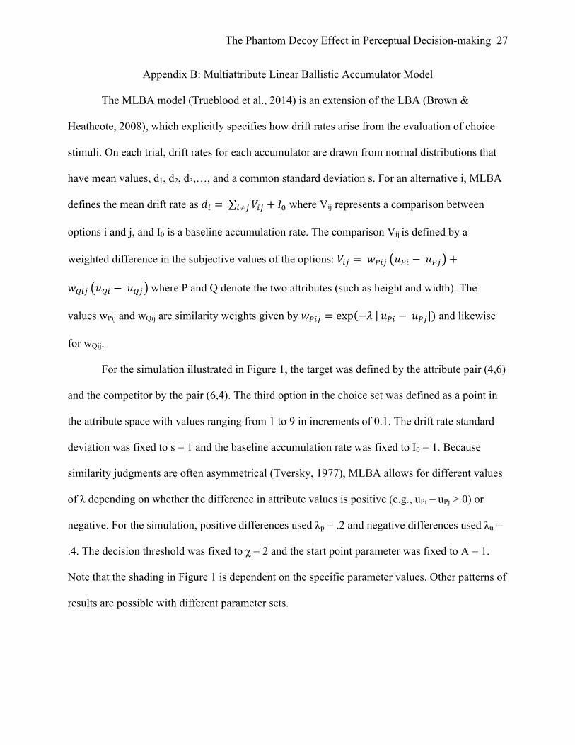
Appendix B: Multiattribute Linear Ballistic Accumulator Model

The MLBA model (Trueblood et al., 2014) is an extension of the LBA (Brown &

Heathcote, 2008), which explicitly specifies how drift rates arise from the evaluation of choice

stimuli. On each trial, drift rates for each accumulator are drawn from normal distributions that

have mean values, d1, d2, d3,…, and a common standard deviation s. For an alternative i, MLBA

defines the mean drift rate as 𝑑! = 𝑉!"!!! + 𝐼! where Vij represents a comparison between

options i and j, and I0 is a baseline accumulation rate. The comparison Vij is defined by a

weighted difference in the subjective values of the options: 𝑉!" = 𝑤!"# 𝑢!" − 𝑢!" +

𝑤!"# 𝑢!" − 𝑢!" where P and Q denote the two attributes (such as height and width). The

values wPij and wQij are similarity weights given by 𝑤!"# = exp −𝜆 𝑢!" − 𝑢!"|) and likewise

for wQij.

For the simulation illustrated in Figure 1, the target was defined by the attribute pair (4,6)

and the competitor by the pair (6,4). The third option in the choice set was defined as a point in

the attribute space with values ranging from 1 to 9 in increments of 0.1. The drift rate standard

deviation was fixed to s = 1 and the baseline accumulation rate was fixed to I0 = 1. Because

similarity judgments are often asymmetrical (Tversky, 1977), MLBA allows for different values

of λ depending on whether the difference in attribute values is positive (e.g., uPi – uPj > 0) or

negative. For the simulation, positive differences used λp = .2 and negative differences used λn =

.4. The decision threshold was fixed to χ = 2 and the start point parameter was fixed to A = 1.

Note that the shading in Figure 1 is dependent on the specific parameter values. Other patterns of

results are possible with different parameter sets.


28

Author’s note

JST was supported by NSF grants SES-1556325 and SES-1556415. The opinions expressed in

this publication are those of the authors and do not necessarily reflect the views of the funding

agencies.


29

References

Anderson, N. H., & Weiss, D. J. (1971). Test of a multiplying model for estimated area of

rectangles. The American Journal of Psychology, 84(4), 543–8.

Berkowitsch, N. A. J., Scheibehenne, B., & Rieskamp, J. (2014). Rigorously testing

multialternative decision field theory against random utility models. Journal of

Experimental Psychology. General, 143, 1331–48. doi:10.1037/a0035159

Bhatia, S. (2013). Associations and the accumulation of preference. Psychological Review,

120(3), 522–543. doi:10.1037/a0032457

Brown, S. D., & Heathcote, A. (2008). The simplest complete model of choice response time:

Linear ballistic accumulation. Cognitive Psychology, 57, 153–178.

doi:10.1016/j.cogpsych.2007.12.002

Busemeyer, J. R., Jessup, R. K., Johnson, J. G., & Townsend, J. T. (2006). Building bridges

between neural models and complex decision making behaviour. Neural Networks  : The

Official Journal of the International Neural Network Society, 19, 1047–58.

doi:10.1016/j.neunet.2006.05.043

Choplin, J. M., & Hummel, J. E. (2002). Magnitude comparisons distort mental representations

of magnitude. Journal of Experimental Psychology: General, 131(2), 270.

Choplin, J. M., & Hummel, J. E. (2005). Comparison-induced decoy effects. Memory &

Cognition, 33, 332–343. doi:10.3758/BF03195321


30

Eriksen, B. A., & Eriksen, C. W. (1974). Effects of noise letters upon the identification of a

target letter in a nonsearch task. Perception & Psychophysics, 16(1), 143–149.

doi:10.3758/BF03203267

Frederick, S., Lee, L., & Baskin, E. (2014). The limits of attraction. Journal of Marketing

Research, 51(4), 487-507.

Gold, J. I., & Shadlen, M. N. (2007). The neural basis of decision making. Annual Review of

Neuroscience, 30, 535–574. doi:10.1146/annurev.neuro.29.051605.113038

Hawkins, G. E., Rae, B., Nesbitt, K. V., Brown, S. D. (2013). Gamelike features may not

improve data. Behavior Research Methods, 45, 301-318. Doi 10.3758/s13428-012-0264-3

Highhouse, S. (1996). Context-dependent selection: The effects of decoy and phantom job

candidates. Organizational Behavior and Human Decision Processes, 65(1), 68-76.

Huber, J., Payne, J. W., & Puto, C. (1982). Adding Asymmetrically Dominated Alternatives:

Violations of Regularity and the Similarity Hypothesis, 9, 90-98. Journal of Consumer

Research. doi:10.1086/208899

Kruschke, J. (2010). Doing Bayesian Data Analysis: A Tutorial Introduction with R. Burlington,

MA: Academic Press.

Lee, M. D., & Wagenmakers, E.-J. (2014). Bayesian Cognitive Modeling: A Practical Course.

Cambridge, UK: Cambridge University Press.


31

Noguchi, T., & Stewart, N. (2014). In the attraction, compromise, and similarity effects,

alternatives are repeatedly compared in pairs on single dimensions. Cognition, 132(1), 44–

56. doi:10.1016/j.cognition.2014.03.006

Parducci, A. (1974). Contextual effects: A range-frequency analysis. Handbook of perception, 2,

127-141.

Pettibone, J. C. (2012). Testing the effect of time pressure on asymmetric dominance and

compromise decoys in choice. Judgment and Decision Making, 7, 513–521.

Pettibone, J. C., & Wedell, D. (2007). Testing Alternative Explanations of Phantom Decoy

Effects. Journal of Behavioral Decision Making, 341, 323–341.

Pettibone, J. C., & Wedell, D. H. (2000). Examining Models of Nondominated Decoy Effects

across Judgment and Choice. Organizational Behavior and Human Decision Processes,

81(2), 300–328. doi:10.1006/obhd.1999.2880

Pratkanis, A. R., & Farquhar, P. H. (1992). A Brief History of Research on Phantom

Alternatives: Evidence for Seven Empirical Generalizations About Phantoms. Basic and

Applied Social Psychology, 13(1), 103–122. doi:10.1207/s15324834basp1301_9

Ratcliff, R. (1978). A theory of memory retrieval. Psychological Review, 85(2), 59-108

doi:10.1037/0033-295X.85.2.59

Roe, R., Busemeyer, J. R., & Townsend, J. T. (2001). Multialternative decision field theory: A

dynamic connectionist model of decision making. Psychological Review, 108(2), 370–392.


32

Scarpi, D., & Pizzi, G. (2013). The Impact of Phantom Decoys on Choices and Perceptions.

Journal of Behavioral Decision Making, 461, 451–461.

Shadlen, M. N., Kiani, R., Hanks, T. D., & Churchland, A. K. (2008). Neurobiology of Decision

Making An Intentional Framework. In Better Than Conscious? Decision Making, the

Human Mind, and Implications For Institutions (pp. 71–101).

Simonson, I. (1989). Choice Based on Reasons: The Case of Attraction and Compromise Effects.

Journal of Consumer Research, 16, 158-174. doi:10.1086/209205

Smith, P. L., & Ratcliff, R. (2004). Psychology and neurobiology of simple decisions. Trends in

Neurosciences, 27(3), 161-168. doi:10.1016/j.tins.2004.01.006

Summerfield, C., & Tsetsos, K. (2012). Building Bridges between Perceptual and Economic

Decision-Making: Neural and Computational Mechanisms. Frontiers in Neuroscience, 6, 1-

20. doi:10.3389/fnins.2012.00070

Symmonds, M., & Dolan, R. J. (2012). The Neurobiology of Preferences. In Neuroscience of

Preference and Choice (pp. 3–31). doi:10.1016/B978-0-12-381431-9.00001-2

Trueblood, J. S. (2015). Reference Point Effects in Riskless Choice Without Loss Aversion.

Decision, 2(1), 13-26. doi:10.1037/dec0000015

Trueblood, J. S., Brown, S. D., & Heathcote, A. (in press). The fragile nature of contextual

preference reversals: Relpy to Tsetsos, Chater, and Usher. Psychological Review.


33

Trueblood, J. S., Brown, S. D., & Heathcote, A. (2014). The multiattribute linear ballistic

accumulator model of context effects in multialternative choice. Psychological Review,

121(2), 179–205. doi:10.1037/a0036137

Trueblood, J. S., Brown, S. D., Heathcote, A., & Busemeyer, J. R. (2013). Not just for

consumers: context effects are fundamental to decision making. Psychological Science, 24,

901–908. doi:10.1177/0956797612464241

Tsetsos, K., Chater, N., & Usher, M. (2012). Salience driven value integration explains decision

biases and preference reversal. Proceedings of the National Academy of Sciences, 109(24),

9659-9664. doi:10.1073/pnas.1119569109

Tsetsos, K., Usher, M., & McClelland, J. L. (2011). Testing multi-alternative decision models

with non-stationary evidence. Frontiers in Neuroscience, 5. doi:10.3389/fnins.2011.00063

Tversky, A. (1972). Elimination by aspects: A theory of choice. Psychological review, 79(4),

281-299.

Tversky, A. (1977). Features of similarity. Psychological Review, 84(4), 327-352.

doi:10.1037/0033-295X.84.4.327

Tversky, A., & Simonson, I. (1993). Context-Dependent Preferences. Management Science,

39(10), 1179-1189. doi:10.1287/mnsc.39.10.1179

Usher, M., & McClelland, J. L. (2004). Loss aversion and inhibition in dynamical models of

multialternative choice. Psychological Review, 111, 757–769. doi:10.1037/0033-

295X.111.3.757


34

Wedell, D. H., & Pettibone, J. C. (1996). Using Judgments to Understand Decoy Effects in

Choice. Organizational Behavior and Human Decision Processes, 67, 326–344.

doi:10.1006/obhd.1996.0083

Wedell, D. H., & Pettibone, J. C. (1999). Preference and the contextual basis of ideals in

judgment and choice. Journal of Experimental Psychology: General, 128(3), 346-361.

Wollschläger, L. M., & Diederich, A. (2012). The 2N-ary Choice Tree Model for N-Alternative

Preferential Choice. Frontiers in Psychology, 3. doi:10.3389/fpsyg.2012.00189

Yechiam, E., & Hochman, G. (2013). Loss-aversion or loss-attention: The impact of losses on

cognitive performance. Cognitive Psychology, 66, 212–231.

doi:10.1016/j.cogpsych.2012.12.001


35

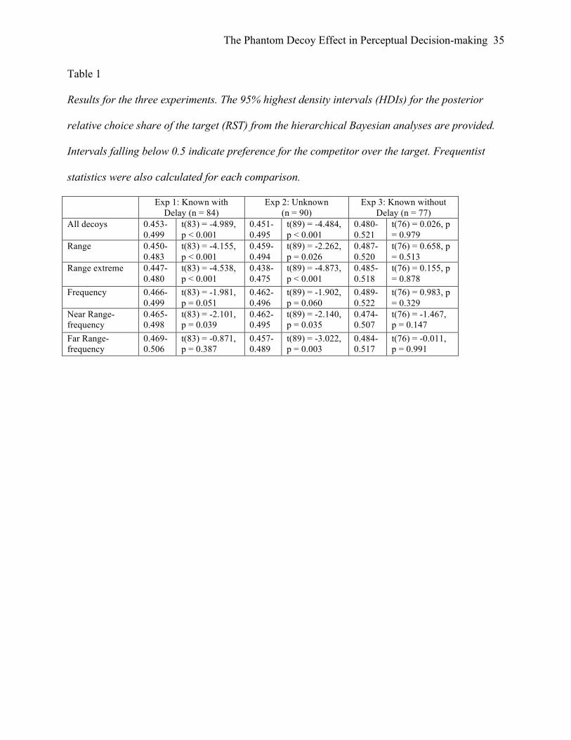
Table 1

Results for the three experiments. The 95% highest density intervals (HDIs) for the posterior

relative choice share of the target (RST) from the hierarchical Bayesian analyses are provided.

Intervals falling below 0.5 indicate preference for the competitor over the target. Frequentist

statistics were also calculated for each comparison.

Exp 1: Known with Delay (n = 84)

Exp 2: Unknown (n = 90)

Exp 3: Known without Delay (n = 77)

All decoys 0.453-0.499

t(83) = -4.989, p < 0.001

0.451-0.495

t(89) = -4.484, p < 0.001

0.480-0.521

t(76) = 0.026, p = 0.979

Range 0.450-0.483

t(83) = -4.155, p < 0.001

0.459-0.494

t(89) = -2.262, p = 0.026

0.487-0.520

t(76) = 0.658, p = 0.513

Range extreme 0.447-0.480

t(83) = -4.538, p < 0.001

0.438-0.475

t(89) = -4.873, p < 0.001

0.485-0.518

t(76) = 0.155, p = 0.878

Frequency 0.466-0.499

t(83) = -1.981, p = 0.051

0.462-0.496

t(89) = -1.902, p = 0.060

0.489-0.522

t(76) = 0.983, p = 0.329

Near Range-frequency

0.465-0.498

t(83) = -2.101, p = 0.039

0.462-0.495

t(89) = -2.140, p = 0.035

0.474-0.507

t(76) = -1.467, p = 0.147

Far Range-frequency

0.469-0.506

t(83) = -0.871, p = 0.387

0.457-0.489

t(89) = -3.022, p = 0.003

0.484-0.517

t(76) = -0.011, p = 0.991


36

Figure Captions

Figure 1. Placements of the standard asymmetrically dominated range decoy (ADR),

compromise decoy (COM), phantom range decoy (PR), phantom extreme range decoy (PER),

phantom frequency decoy (PF), phantom near range-frequency decoy (PnRF), and phantom far

range-frequency decoy (PfRF). The range phantom (PR) serves to increase the range of

evaluation along the best dimension of the target while sharing its value on the worst dimension.

The extended range phantom (PER) is similar to the range phantom but extends the range of

evaluation on the target’s best dimension further. The frequency phantom (PF) is placed between

the target and the competitor on the worst attribute of the target while sharing its best attribute.

The range-frequency phantom, shown here in near to the target (PnRF) and far from the target

(PfRF) versions, combines both the range and frequency manipulations. All decoys target

alternative T = (4,6) over alternative C = (6,4). The dotted lines represent the equi-

preference/size contours given equal weighting of the dimensions. The shade at each point

reflects the RST when the decoy at that location is included in the choice set as calculated using

the MLBA model (see Appendix B). Darker shades indicate increased preference for the

competitor over the target.

Figure 2. An example of a trial from Experiment 1. Participants first viewed the information

shown in the panel on the left for 2 seconds. Then, the screen was updated to show the

information presented in the right panel. Participants could make their decision anytime after the

update in information.

Figure 3. Hierarchical Bayesian model used to test whether the RST values were larger or

smaller than 0.5 for the phantom decoy effect. Circular nodes indicate continuous values, square

nodes indicate discrete values, shaded nodes correspond to known values, and unshaded nodes


37

represent unknown values. The bounding rectangles are called plates and are used to enclose

independent replications of a graphical structure. There are two plates in the figure representing

replications for the five different types of decoys (outer plate) and replications for different

individuals (inner plate). The nodes labeled ϕj and κj (j = 1…5) are the hyperparameters for each

decoy type. Each individual has five θ parameters, which are drawn from beta distributions

determined by the hyperparameters. The ϕj parameters also follow a beta distribution with

parameters µϕ and κϕ, which captures the group-level effect across all five decoys combined.

Figure 4. Mean choice proportions for the target and competitor options averaged over five

decoy locations for three different experiments, which manipulate the time when the phantom

decoy is announced as unavailable. The mean and the standard error of the mean are shown

above each bar.


38

Figure 1.

Dimension 1

Dim

ensi

on 2

1 2 3 4 5 6 7 8 9

9

8

7

6

5

4

3

2

10.1

0.2

0.3

0.4

0.5

0.6

0.7

0.8

0.9

T

PR

PER

PF

PnRF

PfRF

C

ADR

COM


39

Figure 2.

Here are the possible plots. Select the plot you prefer.

2 3 unavailable


40

Figure 3.

µφ κφ

φj

κj θij

Tij

Tij + Cij

j = 5 effects

i = 1, . . . , N

µφ ∼ Beta!

2, 2"

κφ ∼ Gamma!

0.001, 0.001"

αφ = µφκφ

βφ = (1− µφ)κφ

φj ∼ Beta!

αφ,βφ

"

κj ∼ Gamma!

0.001, 0.001"

αj = φjκj

βj = (1− φj)κj

θij ∼ Beta!

αj ,βj

"

Tij ∼ Binomial!

θij , Tij + Cij

"


41

Figure 4.

Known with Delay Unknown Known without Delay0.3

0.4

0.5

0.6

Choic

e Pr

opor

tions

TargetCompetitor

.52 ( .004)

.48 ( .004)

.52 ( .004)

.47 ( .004).50 ( .004) .50 ( .004)

the phantom decoy effect in perceptual decision · pdf filethe phantom decoy effect in...

Documents