The Political Economy of Financial Repression

in Transition Economies

Cevdet DenizerThe World Bank

Raj M. DesaiGeorgetown University

Nikolay GueorguievInternational Monetary Fund

September 1988

2

THE POLITICAL ECONOMY OF FINANCIAL REPRESSIONIN TRANSITION ECONOMIES

Cevdet Denizer, Raj M. Desai, and Nikolay Gueorguiev1

I. INTRODUCTION

Why do governments distort financial markets and impose impediments to capital mobilitydespite the inefficiencies that accompany such policies? It is well known that financial systems indeveloping countries tend to be “restricted” or “repressed” through burdensome reserverequirements, through interest-rate ceilings, through foreign-exchange regulations, through rulesgoverning the composition of bank balance sheets, or through forms of heavy taxation of thefinancial sector. Less understood is why governments are drawn to regulate financial markets to thepoint of financial repression.

Before the 1970's, financial restrictions were often favored in capital-scarce countries on thegrounds that usury could be better prevented, money supply better controlled, and higherinvestment-savings targets met than if financial markets were liberalized. In later years this claimwas frequently supported with evidence from high-growth economies in East Asia, wheregovernments supposedly manipulated financial systems in order to promote targeted industrialexpansion. In most of the settings where repressive financial controls have been applied, however,the typical outcome has been economic contraction, not sustained growth. This realization has ledto the emergence of something of a consensus in development macroeconomics: that financialrepression is adopted in developing countries in order for governments to obtain resources tofinance their deficits.

1. Contact: Raj M. Desai, at Desair@gunet.georgetown.edu A previous version of this paper was prepared for

delivery at the annual meeting of the American Political Science Association, Washington, D.C., 1997. We thank OyaCelasun for invaluable research assistance. The electoral data used in this paper were provided by Joel Hellman andprepared by Joshua Tucker, whom we thank for making this resource available to us. The findings, interpretations, andconclusions presented in this paper are the authors’ own and should not be attributed to The World Bank and IMF, theirExecutive Boards of Directors, their member countries or affiliated institutions.

In this paper we explore some preliminary evidence from a region of the world wherefinancial regulations have rarely been examined in any systematic manner, namely, the post-Communist economies of Eastern Europe and the former Soviet Union. We show that the public-finance framework has limited cache in explaining financial repression in the transition economies,given the peculiar financial lineages of the socialist state. Specifically, the weak distinction betweenthe "public" and "private" spheres of finance in transition economies means that the deficit oftenconveys little information about the real fiscal activities of governments. We find that a more

3

fruitful approach lies in examining how political institutions, by shaping the incentives politiciansface, can determine the choice of financial policy. Our findings suggest that post-Communistgovernments inhibit the development of financial institutions to ensure adequate flows of externalcapital to the enterprise sectors, rather than to finance deficits.

The discussion is organized as follows. Section II defines financial repression, its historicaldebates and rationales. Section III examines the role of financial repression in the unique case oftransition economies. The fourth section presents the empirical results of our estimations offinancial repression in transition economies. The final section summarizes and offers someconcluding remarks.

II. FINANCIAL REPRESSION AND FINANCIAL DEVELOPMENT

Financial Policies and Some Key Issues

For the past 25 years, the main analytical basis for studies of the role of the financial sectorin development has been the McKinnon-Shaw framework of the “repressed” economy. In thisview financial repression refers to a set of policies, laws, formal regulations, and informal controls,imposed by governments on the financial sector, that distort financial prices— interest rates andforeign exchange rates— and inhibit the operation of financial intermediaries at their full potential. The main instruments of financial repression are high reserve requirements and interest-rateceilings, that is, a combination of (forced) low rates of return on assets and (forced) high portionsof “set-aside” or reserve money. Successful financial repression increases the demand for credit,and at the same time, creates disincentives to save.

These conditions permit governments to intervene in financial markets in three ways. First,the imposition of large reserve or liquidity requirements on commercial banks creates an artificialdemand for a government’s own securities (Agénor and Montiel, 1996: 152). Second, because ofthe excess demand for credit, the government invariably begins to ration credit among competingusers. Third, because of the disincentive to save, savers begin to switch from holding claims on thebanking sector to holding claims in foreign markets. Thus selective and sectoral credit schemes, aswell as capital controls on foreign exchange, are typical components of financial repression.

In the neo-classical perspective, the main justification for financial repression derives froman assumption of perfect substitutability of money and “productive” capital. In Tobin’s monetary-growth model, if the return on capital rises relative to the return on money, it encourages a shiftfrom money to capital in household portfolios, higher capital-to-labor ratios, and increased laborproductivity (Tobin, 1965). The central implication of this reasoning is that reducing the rate ofreturn on money— through interest-rate ceilings, but also through an optimal level of inflation, bothof which serve as a tax on real money balances— can increase the rate of economic growth.

McKinnon (1973) and Shaw (1973), however, questioned the applicability of the neo-classical approach to developing countries, and instead argued that the distortions from financialrepression crowd out high-yielding investments, create a preference for capital-intensive projects,discourage future saving, and thereby reduce both the quality and quantity of investment in an

4

economy. In this framework, money and capital are compliments rather than substitutes: the moreattractive it is to hold real money balances, the greater the incentive to invest. Productiveinvestment, and therefore capital accumulation, occurs because a large real money stock makesgreater amounts of loanable funds available to borrowers (McKinnon, 1973: 59-61; Shaw, 1973: 81). Expanded financial intermediation between savers and investors, in this view, increases theincentives to save and invest, and improves the efficiency of investment (Fry, 1982: 734). In afinancially repressed economy a low real deposit rate of interest shrinks the liabilities of the bankingsystem (as savers move away from claims on banks), as it does the supply of investment finance. Extensions of the McKinnon-Shaw framework have generally suggested that raising interest rates toequilibrium levels will increase the rate of economic growth.

Financial Repression and Market Failure

In the 1980s, critics of the McKinnon-Shaw framework argued that raising institutionalinterest rates might have strong negative effects on savings, investment, output, and growth. Usingmodels incorporating informal credit or “curb” markets, critics of financial liberalization argued thatthe lack of effective institutions in developing countries required some degree of governmentcontrol to be maintained over the financial sector (Taylor, 1983; Van Wijnbergen, 1983a, 1983b;Buffie, 1984). The experience of the newly industrializing East Asian economies played a large partin challenging the wisdom of the McKinnon-Shaw framework, suggesting that governmentintervention in financial markets could be welfare-enhancing (Van Wijnbergen, 1985; Amsden,1989; Wade, 1990). A complimentary finding from analyses of financial liberalization in LatinAmerica was that lifting government controls, in the absence of adequate regulation, could make afragile economic situation worse (Edwards, 1984; Díaz-Alejandro, 1985; Hastings, 1993).

Proponents of “optimal” financial repression have argued that financial controls can correctmarket failures in financial markets, lower the cost of capital for companies, and improve the qualityof loan applicants by selecting out high-risk projects. In addition, if used in conjunction withexport-promotion schemes, or preferential credit schemes, financial repression could encourage theflow of capital to sectors with beneficial technological spillovers (Stiglitz, 1989, 1994). Of course,there are worlds of difference between the claims that financial repression can be efficient and that itwill be. Although research on credit controls in Japan, South Korea, and Taiwan indicated thatfinancial repression contributed to the high performance of those economies, this evidence remainssomewhat controversial. Moreover, the balance of more systematic, cross-national empiricalevidence suggests that there are negative correlations between low real interest rates, high reserverequirements, and low degrees of financial intermediation on one hand, and investment and growthon the other.2

The Public-Finance Approach

Most scholars of finance and development have rejected the claim that financial repressionis adopted on welfare-maximizing grounds alone. Rather, development macro economists have,

2. Studies establishing this relationship are: Lanyi and Saraco_lu, 1983; World Bank, 1989; Roubini and Sala-i-Martin 1992; Easterly, 1993; Levine, 1993; King and Levine, 1993a, 1993b. See Levine, 1996 for a review.

5

generally speaking, reached a strong consensus regarding the reasons for financial repression: fluctuations in government revenue. A financial sector under administratively-imposed restrictionsis a potential source of “easy money” for the public budget. In the classic cases of financialrepression, the proliferation of financial instruments from which governments can extractseignorage is encouraged, mainly a relatively oligopolistic banking system, since obligatory holdingsof government bonds can be imposed on commercial banks. Private securities markets aresuppressed through a variety of taxes and duties, since seignorage cannot be so easily extractedfrom these markets (Fry, 1995: 20-22). In short, financial repression has the overall effect oftransferring funds from the financial system to public borrowers.

The “fiscal” choice that governments make in choosing the degree of financial repression,in the public-finance approach, depends on the revenue losses due to the failure of more direct taxinstruments. It has been argued, for example, that economies subject to large amounts of income-tax evasion are likely to turn to implicit taxes in the form of the inflation tax, indirect taxes on thefinancial sector through interest-rate ceilings or high reserve requirements, or some combination ofboth (Roubini and Sala-i-Martin, 1995). In developing countries facing sustained deficits, it isargued, porous or weak systems of revenue collection force governments to rely on inflation taxes. But when governments allow financial systems to develop fully, the need for people to carry moneyis reduced, eroding the inflation tax base, along with the opportunities for seignorage. By enforcingrestrictions on the activities, services, and products of financial institutions, on the other hand,governments can maintain a ready base for the inflation tax.

The implications of the public-finance approach are simple. First, efficient use of theinflation tax requires certain repressive measures to increase the demand for money (Giovanniniand de Melo, 1993; Bencivenga and Smith, 1992; Brock, 1989). Second, everything else being equal,governments that are forced to monetize larger deficits over a longer period of time are more likelyto choose some form of financial repression to augment money demand, but also to allow thedeficit to be financed at a lower interest rate. The question for this paper is: is the public-financeapproach to understanding financial repression justified on theoretical or empirical grounds in thepost-Communist transition economies? We briefly explore both in the next section.

III. FINANCIAL REGULATION IN THEORY AND PRACTICE

Our main conceptual objection to the “easy-money” thesis is that it presents an incompletepicture of the financial-policy choice at the heart of the matter. In assuming that governmentsrespond to potential revenue shortfalls in uniform ways, this approach falls short in explaining whydifferent governments facing similar budgetary constraints might choose to regulate their financialsystems differently. This, more or less, axiomatic depiction of policy-making processes ashomogenous is sharply disputed by research on both the domestic and international aspects offinancial policy-making. Institutional differences among political systems have economic effects;this is a central insight from a quarter-century of research on comparative political economy, as wellas from more recent empirical studies of financial regulation (Quinn and Inclán, 1997), monetarypolicy (Hall and Franzese, 1996; Iversen, 1996), and fiscal policy (Alesina and Rosenthal, 1995). Atbase, financial repression represents a concrete policy choice, and is thus governed by theconstraints and incentives facing policy makers.

6

A more serious objection is that the public-finance explanation for financial repressionrelegates preferential credit policies to a secondary role. In the public-finance view, preferentialcredit schemes are an unintended result of interest rate controls, not their cause. In the standard,hypothetical sequence of events: governments facing a large public sector deficit introduce a varietyof financial restrictions, including interest-rate ceilings, which allow deficit financing at a lowerinterest rate. Since interest-rate controls cause the demand for credit to surge, the government isunwittingly drawn into the process of allocating credit among competing users. A significant bodyof case-study evidence, however, suggests that selective credit schemes are themselves the primaryreasons governments repress their financial systems in the first place (Haggard, Lee, and Maxfield,1993; Lukauskas, 1994; Haggard and Lee, 1996). These are precisely the subjects which are, to us,worth investigating in the context of the post-Communist economies.

Fiscal and Monetary Policy in Post-Communist Economies

The implication that inter-temporal revenue losses may predict the level of financialrepression assumes that the fiscal responsibilities of the state are well-defined and enforceable, andthat any financial flows from the public to the private sector are controlled and appear inconsolidated governmental balance sheets. In other words, "fiscal" property rights are assumed to be exclusive.3 For this reason, the public-finance framework carries little explanatorypower with respect to the formerly state-socialist economies of Central and Eastern Europe and ofthe Former Soviet Union.

In practice, of course, all governments can engage in a variety of activities that render"deficits" meaningless numbers. Unbudgeted expenditures, outside the supervision of budgetoffices, are typical culprits in developing countries (Pradhan, 1996; Campos and Pradhan, 1996). Other quasi-fiscal expenditures include: implicit subsidies with foreign-exchange guaranteeschemes, and implicit subsidies from the provision of credit to banks and firms at negative interestrates. In the post-Communist transition economies, moreover, financial repression may be usedless as a source of cheap money for public deficits, than as a means of maintaining a soft bankingsystem which essentially absorbs enterprise losses in the short run.

Certain legacies of the socialist financial system suggest this possibility. First, bankingsectors remain among the more state-controlled parts of these economies, with few governmentshaving taken steps towards their full commercialization. Thus the line between "public" and"private" finance often remains blurry, with governments prompting banks to act as quasi-fiscalagents of the state through interest-rate controls or, more directly, through directed creditprograms. Second, even in the few cases where banks have been fully or partially commercialized,the lending portfolios that formerly state-owned commercial banks have inherited are heavilyconcentrated among a few firms or industrial sectors. In addition, all formerly state-owned banksinherited bad loans from their public enterprise clients— loans that continue to list on the asset sideof their balance sheets. Under such circumstances, foreclosing on the biggest borrowers oftenthreatens the banks themselves (Desai and Pistor, 1997). Finally, the enforcement of debt

3. On the concept of "fiscal" property rights, see Tanzi, 1993a, 1993b.

7

contracts, in most cases, is impaired due to the incapacity of courts, ambiguities in bankruptcylegislation, and ad hoc government interventions on behalf of certain companies.4

4. Over the long run, of course, the inability of insolvent enterprises to make payments on loans should lead

commercial banks to cut them off as clients. But in the short term, these factors peculiar to the transition economies mayactually encourage banks to lend more, rather than less, to loss-making firms.

While it is difficult to estimate the size of directed credits from the banking systems intransition economies in a reliable way, the experience of Russia is indicative as to how large they canbe. Easterly and Vieira da Cunha Cunha (1994), for example, show rapid inflation in Russia erodedthe financial savings of households and it was this group that paid the inflation tax. Their estimatessuggest that the losses of households becasue of highly negative interest rates, about -78 percent, in1992 were about 12 percent of Russian GDP. Enterprises, like anybody who had bank deposits,also lost and their losses were about 18 percent of GDP in 1992. However, as the RussianGovernment issued credit to enterprises this sector was a beneficiary of inflationary financing.Easterly and Vieira da Cunha's estimates suggest that the amount they received in 1992 was about16 percent of GDP with their net inflaton tax being only 2 percent as opposed to 12 percent by thehouseholds. Hence, the costs of financial repression has been large, at least in Russia and there werelarge income transfers from one group to another.

8

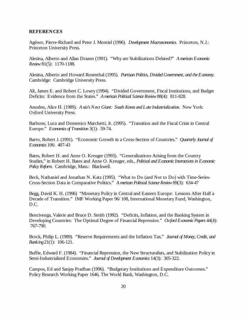
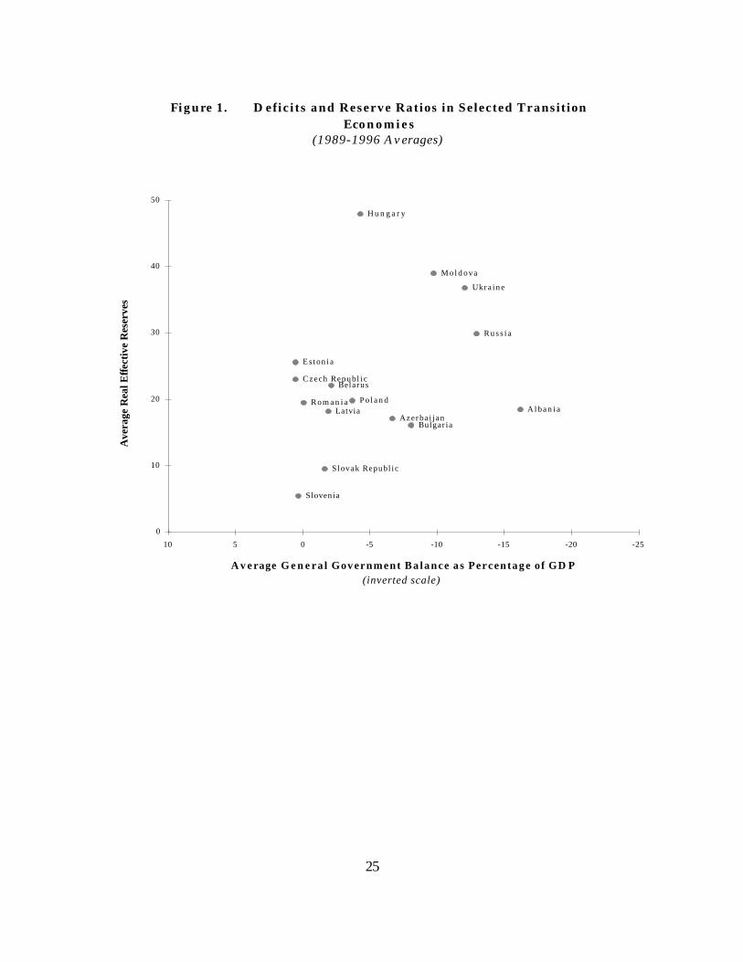
One might expect deficits and revenue losses to be an overriding concern of post-Communist governments, most of which have witnessed tax-evasion epidemics following thedismantling of the socialist revenue-collection apparatus, the multiplication of taxpayers followingprivatization, and the fall in information available to tax authorities (Barbone and Marchetti, 1995;IMF, 1995).5 Meanwhile, just as public finances were being restructured, governments in thisregion faced their most severe budgetary pressures in decades, as they were forced to assumespending responsibilities that previously were fulfilled by enterprises— pensions, medical care, andwelfare. If these revenue concerns were the primary reason for adopting restrictive controls on theactivities of financial intermediaries, then the inflation tax should have been used in conjunctionwith these restrictions in the transition countries, as the public-finance approach hypothesizes. Agraphic illustration of the relationship between reserves in the banking system (an indicator offinancial repression) and deficits between 1989 and 1996 reveals no clear-cut answer. The scatter-plot (Figure 1) shows two "clusters" of countries, the first in the lower left-hand portion of thechart, the second farther to the upper-right. But within each of these clusters, one might also see anegative relationship between size of the deficit and reserve ratios. The lack of data impair a moresystematic evaluation of this kind.

5. Revenue collection in the classic socialist system was facilitated to a great extent by the unitary organization of

the Party-state, and the relatively small number of tax instruments— namely, turnover, profit, and payroll taxes securedfrom a small number of large state-owned enterprises under the supervision of branch directorates. For a description, seeKornai, 1992; Garvy, 1977.

We examine some hypothesized relationships between financial restrictions and certainfiscal indicators as a second test of the general public-finance framework. The resultingcorrelations, based on annual data from 25 transition economies, are presented in table 1. Tworesults seem to confirm the public finance thesis: (i) that tax losses are associated with higher realreserve ratios in deposit-taking banks; and (ii) positive fiscal balances are associated with higher realdiscount rates. These correlations, however— based on ccountry-year observations--hide what is, tous, both counterintuitive and worth explaining, namely, cross-country differences. In table 2,therefore, we replicate a methodology used by Brock (1989) for some transition economies. Thefirst four columns show means and standard deviations, respectively, for inflation and real effectivereserve ratios, both of which are calculated monthly for as many months as are available in theIMF's International Financial Statistics monthly tables in order to maximize the number ofobservations. Only thirteen of twenty-five transition economies report both inflation and thedifferent monetary values needed for the real effective reserve ratio calculation. The fifth and sixthcolumns show simple correlations and their corresponding level of significance for each country. Of the thirteen values, we find seven which are significant at or above 95% confidence— foursuggesting a positive relationship between inflation and real reserves, and three showing a negativerelationship. In Brock's original table, the results (calculated from annual, rather than monthlyfigures) for selected countries in both the developing world and in industrialized nations suggested agenerally robust positive, significant correlation between inflation and bank reserves. Evidencefrom the transition economies, on the other hand, is at best inconclusive on the relationshipbetween the inflation tax and financial repression.

9

Finally, for the same thirteen countries, we list maximum and minimum annual real centralbank discount rates for the period 1990-1996 in table 3. This table also lists the rank correlationsbetween real discount rates and net government credit on the basis of quarterly IMF figures. Incomparison to table 2 above, the correlations generated here are weaker; none of them aresignificant above the 99% confidence level. More importantly, of the five correlations significant ator above the 90% level only one (Estonia) supports the public-finance hypothesis that lower realdiscount rates encourage greater government borrowing.

We propose an alternative approach to understanding financial regulation. Our aim here isto provide, as much as possible, a systematic analysis of the political economy of financialliberalization in the post-Communist region, explaining how different policy decisions are reachedin different political settings.

Modeling the Politics of Financial Policy

Recent studies of how political institutions shape economic policy are of two views. In thefirst view, two features of political systems matter: stability and polarization. Unstablegovernments are claimed to behave more "myopically", that is, discount the future at a greater ratethan more cohesive systems, while polarized governments exacerbate the coordination problemsinherent in adopting economic reforms and lead to protracted stalemates (Rodrik, 1993).

Governments that are more likely to be thrown out in future elections, and governmentsthat are characterized by divisive and sharp disagreements between alternative policy makers,therefore, are more likely to delay the adoption of stabilization programs (Alesina and Drazen,1991), and especially more likely to run higher deficits (Roubini and Sachs, 1989; Alt and Lowry,1994; Grilli, Masciandaro, and Tabellini, 1995). It has been suggested that such explanations ofeconomic policy do not show much affection for the procedural or structural features ofdemocratic government, namely, decentralization, electoral competition, and divided government. Fragmented governments also fall prey to anti-reform forces and vested interests, which canmobilize to block reform programs more easily than if power were consolidated in highlyautonomous governmental institutions. Comparative cases studies of reform episodes suggest thatcentralized authority, unified party systems, and strong executives are what typically characterize thepolitical basis for economic adjustment (Nelson, 1990; Haggard and Webb, 1993; Williamson, 1994;Haggard and Kaufman, 1995).

A more recent, second view has challenged the argument that strong, centralizedgovernments are needed for liberalization. This alternative view suggests that economic reforms area by-product of struggles for political authority, and thus the major obstacle to economicliberalization is not the stalemate among groups fighting over the distribution of costs and benefitsof reforms, but the internal opposition to such reforms within governments. Thus reforms are morelikely to occur when political outsiders challenge the authority of incumbents (Bates and Kreuger,1993; Geddes, 1994; Hellman, forthcoming). Accordingly, the structure of political institutions,which determines how internal governmental struggles will be borne out, and how competinginterests will be articulated, play a critical role in shaping policy outcomes.

This second approach has been used to explain stabilization delays in the case of thetransition economies. Hellman (forthcoming) examines the effects of party fragmentation,coalition structure, and executive power on the "survival" rates of inflationary periods, and finds

10

that those countries whose political institutions are characterized by fragmented parliaments, multi-party coalition governments, and weak executives, stabilize faster than those countries with unifiedparty structures, majority or single-party governments, and authoritarian executives. In the sectionthat follows, we analyze the impact of different political structures on financial policy and financialliberalization, focusing on three main institutional features of legislatures in twenty-five transitioncountries: the share of seats held by the Communist Party or its direct descendants, the degree ofparty fragmentation, and the degree of parliamentary support for the government in power.

The first measure we consider to be an approximation of anti-reform incumbent power, thesecond to be a measure of polarization, the third a measure of expected stability. FollowingHellman, we consider the effect of each institutional feature on financial repression separately, inorder to test specific, broader hypotheses about the relationship between the characteristics ofpolitical institutions and economic policies. The financial policies of transition countries havedisplayed a great deal of variation between 1989 and 1996 (World Bank, 1996; Begg, 1996); thecauses of this variation, and particularly the links between political-institutional variables and policyoutcomes have yet to be analyzed in a comprehensive way.

IV. DATA, MODELS, AND RESULTS

Measuring Financial Repression

Financial repression is a reference to a specific set of policies involving a variety of controlson the activities of the main financial institutions in an economy. The analysis of such policies,however, does not easily lend itself to systematic study. First, financial restrictions may be implicit,imbedded in intricate tax codes or financial regulations. Second, there are also problems of codingsuch policies across countries in a way that is standard and comparable, especially when thecountries in question lack precedents or conventions needed for “benchmarks” against whichvariation in such policies could be measured. Finally, a financially “repressed” economy may exhibitcertain effects— low interest rates for financial transactions, distortions in savings and investment,and low levels of financial intermediation— that may or may not be attributable to those policies. In table 1 above, for example, there are several countries that maintain extremely high reserves inthe banking system even if the legal reserve requirements are modest. In Hungary, Estonia, and theCzech Republic, real reserve ratios are 48%, 27%, and 20% respectively despite a common 10%required-reserve ratio in each these countries.6 It is therefore desirable to consider a range ofdifferent indicators of financial repression.

Our solution is to examine three different “proxies” for financial repression and financialliberalization, two of which are policies, one of which measures a hypothesized effect of thesepolicies. The first measure is directed credit, which we code as a binary variable. Following earlierstudies, countries in which directed credits constitute more that 25% of the total credit volume inthe economy are assigned a value of one; all others are coded zero (IMF, 1996; de Melo and

6. In several countries, banks often kept reserves in excess of what they were required to hold by law as hedge

against poorly-enforced creditor rights— a consequence of, among other things, deficiencies in bankruptcy laws,lengthiness of court-adjudicated proceedings, and the limited variety of financial instruments that could yield reasonablerisk-adjusted returns.

11

Denizer, 1997). Directed credit programs, used by former socialist governments to maintainemployment levels in certain industries, represent a fairly severe restriction on the portfoliocomposition of banks’ balance sheets. Under the typical directed-credit scheme, banks areinstructed to lend to certain sectors or enterprises a specified portion of their total assets or totallending in a certain time period. These quantitative restrictions, coupled with the interest-ratecontrols often attached to these loans, tend to segment financial markets in these countries, andconstitutes a significant obstacle to their development.

The second dependent variable is the real discount rate used by central banks for theirrefinance operations. Since the discount or refinance rate is a policy measure used at the discretionof the central banks, however, and since it becomes the base rate for other rates, this is likely to bea better indicator of policy stance than deposit or lending rates. We calculate the real central bankdiscount rate as the nominal discount rate deflated by the price level (annualized).

Finally, we choose a third variable to measure the effect of financial repression on the level offinancial intermediation. The most accurate way to gauge these effects would be to estimate a money-demand curve at different periods in time in order to measure shifts in the curve, along withchanges in cost and income elasticity (Fry, 1995: 21). Such an estimation is difficult in the contextof the transition economies due to lack of observations and shortness of time-horizon. We use,instead, the ratio of money supply (defined to include currency in circulation, sight and timedeposits, or M2) to GDP— a standard measure of financial “depth” that is consistently found to behigher in market economies (indicating that most transactions are intermediated within a formalfinancial system) and lower in financially repressed economies (Barro, 1991; King and Levine,1993b).

Explanatory Variables and Estimation

We estimate these four variables using cross-sectional, time-series analysis with country-years as units of observation. Such a pooling of data, in addition to increasing the degrees offreedom, is also more sensitive to the inter-temporal properties of the sample than would be periodaverages for each country. Ours is not, however, a standard panel as only observations for the yearfollowing parliamentary elections are selected, and our electoral variables are lagged once withrespect to the dependent variables. Such matching is preferred to a standard panel given that thedata exhibit limited variation between elections. In a standard panel this would create problemswith standard errors, as one would be trying to approximate a continuous line with a crude stepwisefunction involving fairly long steps. The units of the time series in our panels, therefore, representelectoral periods rather than calendar years. Although we lose data in between elections for thedependent variables (and some independent variables), we maintain all the inter-temporal variationin the sample and eliminate most of the flat segments. (For an explanation of certain estimationproblems and how they were dealt with, see appendix.)

Using the electoral database compiled in Hellman (forthcoming), we calculate threeindicators of parliamentary structure.7 Our first variable is the share of seats in parliament held by

7. A complete set of political-institutional indicators should also, naturally, include some measure of executivepowers. In fact, Hellman (forthcoming) codes the transition countries according to degree of presidential and prime-

12

members of the Communist Party, or its direct descendant or set of descendants (COMMP). Ahigh percentage for COMMP can be interpreted, ceteris paribus, as an indicator of several things,including “insider” control of the legislature, low development of a party system, lack of politicalsuccession in parliament, and so on. In general, then, we consider COMMP to measure the degreeof “persistence” of pre-reform elites in legislatures. To measure the degree of polarization inparliaments, we use the Rae fractionalization index (FRACTION), which measures the likelihoodthat two legislators chosen at random belong to different political parties.8 Inevitably, theFRACTION panel suffers from two defects: it does not control for the sometimes large number ofindependent members of parliament, nor does it include “extra-electoral” changes in partyaffiliation or party unity. Where parties splintered between elections, the increased Rae index isreflected in the next electoral period.9 Finally, we calculate level of parliamentary support for thegovernment by simply adding up all seats that the government coalition can claim, divided by thetotal number of seats in parliament (GOVSTR). This measure may be interpreted as a proxy forgovernment stability, as low values indicate a higher probability, ceteris paribus, that the governmentin power may be removed at some future date.

We hypothesize that the influence of electoral changes should be the strongest within afinite period following an election. Given that elections take part in different months of the year,and that there is a necessary “transition” period of a few months, during which changes in thecomposition of parliaments and government produced by elections occurs, the year of electionwould not be the best choice for the independent variables. After a first full year, moreover, future

ministerial strength, using the methodology in Shugart and Carey (1992). We included these variables in our estimations,but in no specifications did they turn out to be significant, either independently, or in conjunction with the parliamentary-structural variables.

8. The Rae index is defined as:

Install Equation Editor and double-click here to view equation.

where pi is the fractional share of seats of the i-th party (Rae, 1967).9. As Hellman (forthcoming) notes, this is most commonly the case in countries where broad anti-Communist

reform movements won certain critical elections (held in 1990 in Czechoslovakia, Estonia, Latvia, Lithuania Macedonia,Moldova, Romania, Slovenia, 1991 in Russia), but splintered shortly thereafter. In most of these countries, the Rae indexrises following the next electoral period, which occurs within two years in all cases except Latvia (three years) andMacedonia (four years). Only in Lithuania (between 1990 and 1992) and Macedonia (between 1990 and 1994) does thefractionalization number fall. Certainly this may hide— or even worse, reverse— some of the inter-temporal variation thatoccurs, but there is simply no reliable way of accounting for these changes. Part of this problem, however, is solvedthrough our use of “matched” observation panels.

13

electoral considerations may change politicians’ behavior. For these reasons, all of our relevantpolitical variables are lagged once with respect to the dependent variable.

Several conditioning variables have been included to control for certain factors in theregressions (see appendix for data sources): the logarithm of per-capita GNP (based on the WorldBank Atlas method), on the premise that richer nations repress their financial systems less; the ratioof fiscal balance to GDP, to test the public-finance claim that countries with larger deficits willrepress their financial systems more; and the familiar dummy variable, Post-Soviet (coded 1 if thecountry was a constituent of the U.S.S.R., 0 otherwise) to control for political, economic, social, andstructural similarities that former Soviet republics may share.10 In the regressions for financialdepth and the real discount rate, we include the logarithm of the growth in base money to controlfor currency substitution and portfolio switching that is expected during periods of rapid moneygrowth. and attendant inflation. In the directed credit regression, we include Freedom House’sFreedom Index, which ranks countries according to their protection of civil and political liberties, inorder to test the effect of general regime “openness” on state-enterprise relations.11 With theexception of per-capital income (which is lagged once), all conditioning variables arecontemporaneous to the dependent variable.

In sum, our regressions take the following basic formats:

where _i,t is any relevant measure of, alternatively, financial repression or liberalization, Ci,t is avector of contemporaneous conditioning variables, POLi,t-1 is any relevant lagged measure ofparliamentary structure, ß0 is a constant, ß K for K>0 is a coefficient (or vector of coefficients) oneach variable (or vector), ei,t is a random disturbance term, and where i=1,...,N, t=1,...,T for Ncountries and T time periods. To gauge differences in the effects of the political variables betweenthose countries of the former Soviet Union and those countries in Eastern Europe, we test asecond model which disaggregates POLi,t-1 into two interactive terms, one with an East-Europedummy variable (EE) another with the Post-Soviet dummy (FSU). All regressions— with theexception of the directed credit estimation— were performed using ordinary least squares (OLS).

Results

Tables 4, 6, and 7 present our regression results for each of the dependent variables. Intable 4 we report the results for directed credit— generated using the probit method, by which we

10. Following convention, we did not code the Baltic states as “Post Soviet,” on the grounds that this might be anartificial way of inducing intra-Soviet variation into the results. Coding them 1, however, does not alter our resultssignificantly.

11. In this sense the Freedom Index is a proxy for “access” to decision making authority, and its inclusioncontrols for differences across countries.

Install Equation Editor and double-click here to view equation.

Install Equation Editor and double-click here to view equation.

14

estimate the probability a given country will implement a directed credit program. In our firstmodel, both the Freedom Index12 and Communist share of seats are significant. Note that, by itself,COMMP is significant and has the expected (positive) sign. When we split this variable betweenformer Soviet and East European countries we see that only the Post-Soviet, interactive coefficientis significant. This is so even with the inclusion of the Post-Soviet dummy, suggesting a robustresult. In the next step we analyze fractionalization, which carries a significant, negative sign,indicating that fractionalized parliaments are less likely to implement directed credit programs. Fractionalization also has a differential impact between Soviet and non-Soviet states, as it appearsthat party fragmentation does not increase the probability of having a directed program in EastEuropean countries while it does in the former Soviet Union. When we performed similar stepswith the government strength variable we found that this variable did not have explanatory power.

12. Note that in the Freedom Index, freedom is measured on an inverted scale, with lower values implying greater

political freedom.

For the remaining two regressions, therefore, we examine “real” measures— the ratio ofmoney supply to GDP and the central bank real discount rate. We begin with some averages intable 5. For each parliamentary measure we took averages for each country over the entire availabletime period. Next we split the sample into “high” or “low” explanatory categories depending uponwhether the country fell above or below the median. Finally we calculated the correspondingM2/GDP ratio and real discount rate averages for the appropriate sample of countries over thesame time period. These values are listed in table 5, along with the individual countries in theirrespective groups. From this rough picture, we see that a high percentage of seats held by theCommunist Party, a high level of party unity (low fractionalization) in parliament, and a high degreeof government support, all correspond to lower real discount rates, but moderately higher levels offinancial depth; differences in the real discount rates, are far more pronounced than differences inM2/GDP.

To test these relationships more systematically, we focus first on the M2/GDP ratio, andperform the same series of tests as we did for directed credit and liberalization. We first specify,however, an equation that may be considered a test of an “economic” model, and thus include onlythe conditioning variables and the Post-Soviet dummy. As shown in table 5, only Sovietmembership turns out to be significant (with the expected negative sign), while per-capita income,fiscal balance, and base money growth are not. Following the same steps as in the first tworegressions, we individually add variables for Communist Party share of seats, fractionalization, andgovernment strength, decomposing each measure between East-European and Post-Soviet regions.

With the exception of government strength, the coefficient on each measure is significantindividually. Note that the statistically significant coefficients for FRACTION and COMMP carrythe signs we expect from table 5. Indeed, according to our results, countries with legislatureshaving a greater percentage of Communists tend to have higher M2/GDP ratios than countries thatdo not. Upon splitting this variable, it remains significant for the FSU only, although the positiveresult is still surprising, especially when the Post Soviet dummy remains significantly negative. Thiswould suggest that former Soviet countries as a whole tend to have lower M2/GDP ratios, but that

15

within this region, having a larger group of Communists in parliament has a positive effect on theratio. The same is not true of the East European countries, where Communist share of seats hasno significant effect. Hence, using a dummy variable for the former Soviet Union, as isconventionally done, may not be a useful device; our results suggest that there is a significantamount of variation within the Post-Soviet bloc that belies their grouping into a single category. Similarly, parliaments with greater levels of party fragmentation are also associated with lower levelsof financial depth. Note, finally, that per capita income and base money growth are nowheresignificant, and that positive budget balances seem to lead to lower levels of financial intermediation(equations 6 and 7)— again, in contradiction tot he public-finance framework.

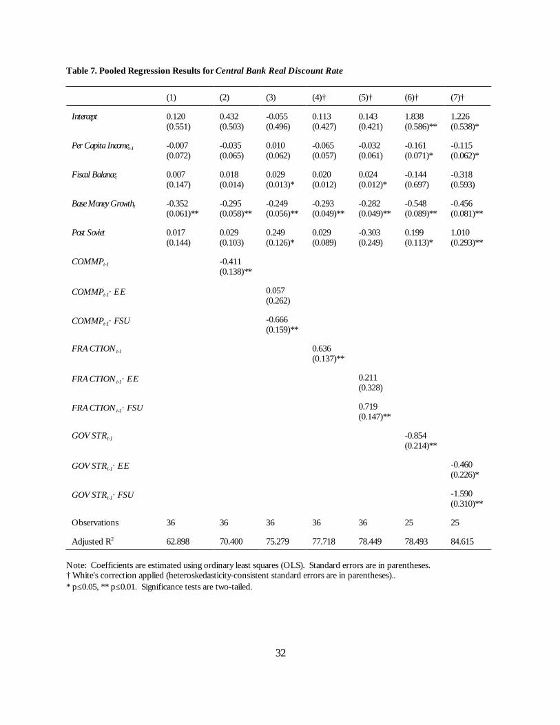
Finally, we turn to the central bank’s real discount rate, presented in table 6. Our baseline“economic” model includes the identical conditioning variables used in the previous set ofregressions: logarithms of per capita income and base money growth, fiscal balance as a proportionof GDP, and a dummy for the former Soviet countries. In this specification, only base moneygrowth is significant. Base money growth, moreover remains strongly negative for all ourspecifications, indicating that an increase in this term— that is, an increase in the rate of base moneygrowth— is correlated with a lower real discount rate, as should be expected. Adding, individually,COMMP, FRACTION, and GOVSTR reveals a common pattern. By themselves, each variablecarries significant coefficients with the signs we expect from table 4. That is, higher shares of seatsheld by Communists and former Communists, greater unity of parties, and greater governmentstrength, all lead to lower real discount rates.

When split between East Europe and the former Soviet Union, these effects are significantfor the latter (the exception is government strength, which is significant in interaction with bothregional dummies). Note again two surprising findings about the former Soviet Union. First, thePost-Soviet dummy, in each specification where it is significant, carries a positive sign. Surprisingly,therefore, this suggests that former Soviet countries have managed to raise their real discount ratesabove that which has been set in non-Soviet countries. Second, in two of the three equationswhere the Post-Soviet dummy is significant (equations 3 and 7) the interactive coefficient carries theopposite sign to the Post-Soviet coefficient. While former Soviet countries may set higher discountrates, within these countries party greater party unity and government strength lead to lower rates. Again, this result suggests that there is a substantial amount of variation in monetary policy withinthe former Soviet Union that is not captured by a single grouping. Ironically, this last set ofregressions leaves the fewest degrees of freedom, but produces the best overall fit.

These results do not lend much support to the thesis that financial liberalization will be lessin politically unstable or polarized systems. The regressions shown here, in fact, suggest that overallfinancial repression is greater in countries with higher percentages of Communists in parliament,less party fractionalization, and greater government support. We see that COMMP andFRACTION are significant for all three dependent variables, GOVSTR for two of them. Moreover, with the exception of our estimation of financial depth, higher COMMP values, lowerFRACTION values, and higher GOVSTR values are correlated with a higher degree of financialrepression.

The role of deficit financing is less conclusive. Certainly, in some specifications, fiscalbalances are significant; in two estimations for M2/GDP and in two estimations for then

16

liberalization index, fiscal balances were correlated with the dependent variable. But in all fourequations, the sign of the coefficient is the opposite of what is expected: larger positive fiscalbalances are correlated with lower levels of financial depth, and with lower degrees of overallliberalization. Moreover it is interesting to note that, in these four equations, only after theGOVSTR variable is added does the government’s fiscal balance generate a significant negativecorrelation, suggesting that the effect of deficits on liberalization and financial liberalization is, to acertain extent, conditioned by the strength of the government. One must allow for the possibilitythat, when one controls for the strength of the government (measured by its parliamentarysupport), deficit-spending governments are more likely to liberalize, and more likely to develop theirfinancial systems. When we control for the other political variables, deficits have no effect. Indeed,we find only two estimations which support the public-finance thesis. In two regression equationsfor the real discount rate, positive fiscal balances were correlated with higher real discount rates. But again, when we control for the strength of the government, the significance of the fiscalbalance coefficient disappears.

V. CONCLUSION: GOVERNMENTS AND FINANCIAL MARKETS

This paper has presented an exploratory analysis of the political correlates of financialrepression in the transition economies. We examined some preliminary evidence for the thesis that,in the face of excessive costs for certain forms of taxation, governments will levy an implicit tax ondomestic financial markets. Such claims were not borne out fully in the data. We suggested thatthe unique lineages of the socialist financial system leave this public-finance framework with limitedapplicability to post-Communist economies.

As an alternative, we outline a rudimentary approach that examines the effects of thedispersion and concentration of political power in governments on financial policy. We find that,for four separate proxies of financial repression, legislatures with larger proportional numbers ofCommunists, with less party competition, and with less governmental opposition, tend to extractrents from financial markets in the form of repressive controls. The most reliable predictors ofwhether governments in transition economies will liberalize financial markets are degree ofCommunist party control and degree of parliamentary polarization, both of which we found to besignificant in most of our specifications. As expected, Communists and their descendants are themost opposed to financial liberalization. But the surprising finding is that polarized, fragmentedparliaments are more likely to liberalize and develop financial systems than those that are moreunified. Finally, government stability, where it was significant, was found to inhibit the liberalizationof financial markets. Our evidence seems to support the view of policy reform predicting thatreform periods will occur as politicians struggle to enhance their authority and snatch the levers offiscal and monetary control away from pre-reform elites.

These findings suggest that repressive financial controls may be adopted not to financedeficits more cheaply than would be the case under financial liberalization, but to maintain theauthority and ensure the survival of those in power. In those countries where pre-reform elites areplentiful in legislative bodies, where inter-party competition is low, and where governing parties arewell-represented in parliaments, elites have been able to perpetuate a system of implicit subsidies by“softening up” the financial sector— particularly the commercial banks— in order to assure the

17

continued flow of cheap credit to specific borrowers. The main beneficiaries of these policies—large formerly state-owned industries with tight financial links to the largest commercial banks— arethus able to convert their well-established claims on public resources into preferential access tocredit lines..

If this is the case, then financial repression serves a special role in transition economies,namely, a mechanism for solidifying main-bank, main-firm relations. Through a combination ofpartial state ownership of financial institutions and interest-rate controls, governments assure thatcommercial banks will maintain the largest enterprises as their chief clients, even once the cashflows of those enterprises have been privatized. In general our results lend some support to thecommon claim of smaller, cash-starved Eastern European entrepreneurs that the commercial bankshave "taken over the role of the old planning ministries."

Our results, finally, revealed a wide degree of variation in the financial policies of the post-Soviet republics, and cast some doubt on the usefulness of generalizations about the former SovietUnion. In addition, one of our more surprising findings was that, in the post-Soviet republics,governments in which Communists are well-represented tend to have "deeper", more developedfinancial systems than the former Soviet countries in which Communists are scarce; this was not,however, the case in the East European countries. This result may belie a non-linear condition inwhat we have attempted to analyze: that there is an optimal degree of former-elite participationneeded for financial reforms, given certain other factors.

If this is true, it suggests a possible explanation for the cross-regional differences betweenthe formerly socialist countries and, for example, Latin America or other developing countries inwhich financial reforms took place after the consolidation of political power, not before— if thoseaccounts are true. It is likely that the conflicts reformers face in setting financial policy— andeconomic policy in general— are conditioned by the peculiar political settings inside which theyoperate, in particular, the relationships between anti-reform elites and existing financial institutions. In the transition economies, the heavy concentration of pre-reform elites in the Communist Party-state apparatus, including the planning bureaucracy and the public-enterprise sector, consisted ofextremely tight relationships between these institutions and a few commercial banks. In such asetting, those forces leading to a general dispersion of political authority— away from a single party,away from the central government, and so on— would more likely lead to successfully implementedfinancial reforms.

By contrast, in countries were the power of anti-reform elites was more decentralized—fragmented along regional, ethnic, or linguistic lines, or where the sources of elite authority weremore closely connected to property ownership— and were financial institutions were regionally-based or specially linked to local industries or landholdings, there it may have been necessary for theopposite to occur, that is, for political authority to be centralized before financial reforms could beimplemented. We can only suggest this possibility here, to mention it briefly, leaving a moresystematic exploration to future research.

18

APPENDIX

Variables, Definitions, Measurement, and Sources(Dependent variables in bold)

Variable Mean (Std. Dev.) Definition Units and Measurement Sources

Directed Credit 0.479 (0.503)

Dummy variable fordirected credit programs

1 if value of directedcredit≥25% of total creditflows, otherwise 0.

1989-1994: de Melo andDenizer (1997); 1995-1996figures calculated on thebasis of central; bankbulletins and IMF staffcountry reports

Financial Depth 0.326 (0.225)

Proportion of financialtransactions in aneconomy intermediatedby formal financialinstitutions

Ratio of broad money (M2) toGDP, in percent.

IMF, International FinancialStatistics (various issues),central bank bulletins, andIMF staff country reports

Real Discount Rate -0.350 (0.412)

Base rate charged tofinancial institution, setat the discretion of thecentral bank

Discount rate n deflated byannualized change in price levelp, in percent:(1+n/1+p)-1

Same as above

COMMP 0.383 (0.311)

Communist Partycontrol in legislature

Share of seats in parliamentheld by members of theCommunist Party or itsdescendant(s), in percent.(lagged)

Calculated on the basis ofdata and in Hellman(forthcoming), updated bythe authors

FRACTION 0.601 (0.271)

Index of partyfractionalization

Herfindahl index of shares ofseats held by all parties inparliament, subtracted fromunity.(lagged)

Same as above

GOVSTR 0.649 (0.192)

Government strength Share of parliamentary seatsheld by party or partiesrepresented in governingcoalition, in percent.(lagged)

Same as above

Post Soviet (FSU-EE) 0.464 (0.502)

Post Soviet and EasternEurope dummies

1 if country was a constituentrepublic of the USSR (with theexception of the Baltic states),otherwise 0 (EE coded in thereverse).

Authors’ coding

Freedom Index 7.466 (3.211)

Index of politicalfreedom(contemporaneous)

Ranks countries from 1(most free) to 14 (least free)

Freedom House, Freedom inthe World (various issues)

19

Variable Mean (Std. Dev.) Definition Units and Measurement SourcesPer Capita Income 2124.6 (1202.9)

Gross national productdivided by population

Log (GNP/Capita), whereGNP is in US$, based on WorldBank Atlas method.(lagged)

World Bank, WorldDevelopment Indicators

Base Money Growth 3.033 (6.909)

Change in moneybalances held bymonetary authorities

Log (1+? M/M),where M is base money.(contemporaneous)

IMF, International FinancialStatistics (various issues),IMF staff country reports

Fiscal Balance -0.320 (2.242)

General governmentconsolidated budgetarybalance

Annual surplus/deficit aspercent of GDP.(contemporaneous)

IMF, Government FinancialStatistics (various issues),IMF staff country reports

Pooled Estimation with “Matched" ObservationsOur technique of matching of independent and dependent variables limits the time-series,

and thus places certain limits on robustness tests. First, we are forced to ignore any possiblecontemporaneous correlation between the same variables for different countries. This would be aproblem in a standard N×T panel for these countries, because N (the number of units) is 25, whileT (the number of time periods) varies between 4 and 6, making it difficult to estimatecontemporaneous correlations. Second, it becomes difficult to test for serial correlation in limitedT panels. We experimented estimating a single first-order autocorrelation coefficient by amaximum likelihood method, but it did not turn out to be significant in any specification. Third, itis also difficult to test for so-called ‘panel heteroskedasticity’, where observations for the same unitare assumed to be homoskedastic, but different units may have different variances (Beck and Katz,1995). As an admittedly imperfect substitute, we applied the White and the Breusch-Pagan tests forheteroskedasticity. Note that these tests are more general, because their alternative hypothesis isthat every observation will have different variances; clearly, “panel heteroskedasticity” would not berejected by this test. With only one exception at 10% confidence level, these tests could not rejectthe null of homoskedasticity, so estimation is performed by standard OLS. In the one case wherethere was suspicion of heteroskedasticity, White’s correction is applied, modified for small samples.

20

REFERENCES

Agénor, Pierre-Richard and Peter J. Montiel (1996). Development Macroeconomics. Princeton, N.J.: Princeton University Press.

Alesina, Alberto and Allan Drazen (1991). “Why are Stabilizations Delated?” American EconomicReview 81(5): 1170-1188.

Alesina, Alberto and Howard Rosenthal (1995). Partisan Politics, Divided Government, and the Economy. Cambridge: Cambridge University Press.

Alt, James E. and Robert C. Lowry (1994). “Divided Government, Fiscal Institutions, and BudgetDeficits: Evidence from the States.” American Political Science Review 88(4): 811-828.

Amsden, Alice H. (1989). Asia’s Next Giant: South Korea and Late Industrialization. New York: Oxford University Press.

Barbone, Luca and Domenico Marchetti, Jr. (1995). “Transition and the Fiscal Crisis in CentralEurope.” Economics of Transition 3(1): 59-74.

Barro, Robert J. (1991). “Economic Growth in a Cross-Section of Countries.” Quarterly Journal ofEconomics 106: 407-43

Bates, Robert H. and Anne O. Kreuger (1993). “Generalizations Arising from the CountryStudies,” in Robert H. Bates and Anne O. Kreuger, eds., Political and Economic Interactions in EconomicPolicy Reform. Cambridge, Mass.: Blackwell.

Beck, Nathaniel and Jonathan N. Katz (1995). “What to Do (and Not to Do) with Time-Series-Cross-Section Data in Comparative Politics.” American Political Science Review 89(3): 634-47

Begg, David K. H. (1996) “Monetary Policy in Central and Eastern Europe: Lessons After Half aDecade of Transition.” IMF Working Paper 96/108, International Monetary Fund, Washington,D.C.

Bencivenga, Valerie and Bruce D. Smith (1992). “Deficits, Inflation, and the Banking System inDeveloping Countries: The Optimal Degree of Financial Repression.” Oxford Economic Papers 44(4): 767-790.

Brock, Philip L. (1989). “Reserve Requirements and the Inflation Tax.” Journal of Money, Credit, andBanking 21(1): 106-121.

Buffie, Edward F. (1984). “Financial Repression, the New Structuralists, and Stabilization Policy inSemi-Industrialized Economies.” Journal of Development Economics 14(3): 305-322.

Campos, Ed and Sanjay Pradhan (1996). “Budgetary Institutions and Expenditure Outcomes.” Policy Research Working Paper 1646, The World Bank, Washington, D.C.

21

de Melo, Martha, Cevdet Denizer, and Alan Gelb (1996). “From Plan to Market: Patterns ofTransition.” World Bank Economic Review 10(3): 397-424.

de Melo, Martha and Alan Gelb (1997). “A Comparative Analysis of Twenty-Eight TransitionEconomies in Europe and Asia.” Post-Soviet Geography and Economics 37(5): 265-285.

de Melo, Martha and Cevdet Denizer (1997). “Monetary Policy during Transition: An Overview.” Policy Research Working Paper 1706, The World Bank, Washington, D.C.

Desai, Raj M. and Katharina Pistor (1997). “Financial Institutions and Corporate Governance,” inIra W. Lieberman, Stilpon S. Nestor, and Raj M. Desai, eds., Between State and Market: MassPrivatization in Transition Economies. Washington, D.C.: The World Bank.

Díaz-Alejandro, Carlos (1985). “Goodbye Financial Repression, Hello Financial Crash.” Journal ofDevelopment Economics 19(1-2): 1-24.

Easterly, William (1993). “How Much do Distortions Affect Growth?” Journal of Monetary Economics32(4): 187-212.

Edwards, Sebastián (1984). “The Order of Liberalization of the External Sector in DevelopingCountries.” Princeton Essays in International Finance 156, Princeton University, Princeton, N.J.

Fry, Maxwell J.(1995). Money, Interest, and Banking in Economic Development, 2nd Ed. Baltimore: JohnsHopkins University Press.

— — — (1982). “Models of Financially Repressed Developing Economies.” World Development10(9): 731-750.

Garvy, George (1977). Money, Financial Flows, and Credit in the Soviet Union. Cambridge, Mass.: Ballinger.

Geddes, Barbara (1994). “Challenging the Conventional Wisdom.” Journal of Democracy 5(October): 104-118.

Giovannini, Alberto and Martha de Melo (1993). “Government Revenue from FinancialRepression.” American Economic Review 83, (4): 953-963.

Grilli, Vittorio, Donato Masciandro, and Guido Tabellini (1995). “Political and MonetaryInstitutions and Public Financial Policies in the Industrial Countries,” in Torsten Persson andGuido Tabellini, eds., Monetary and Fiscal Policy, Vol. 2. Cambridge, Mass.: MIT Press.

Haggard, Stephan, Chung H. Lee, and Sylvia Maxfield, eds. (1993). The Politics of Finance in DevelopingCountries. Ithaca, N.Y.: Cornell University Press.

22

Haggard, Stephan and Steven B. Webb (1993). “What Do We Know About the Political Economyof Economic Policy Reform?” World Bank Research Observer 8(2): 143-168.

Haggard, Stephan and Robert R. Kaufman (1995). The Political Economy of Democratic Transitions. Princeton, N.J.: Princeton University Press.

Hall, Peter A. and Robert J. Franzese, Jr. (1996). “Mixed Signals: Central Bank Independence,Coordinated Wage-Bargaining, and European Monetary Union.” Unpublished.

Hastings, Laura (1993). “Regulatory Revenge: The Politics of Free-Market Financial Reforms inChile,” in Stephan Haggard, Chung H. Lee, and Sylvia Maxfield, eds., The Politics of Finance inDeveloping Countries. Ithaca, N.Y.: Cornell University Press.

Hellman, Joel S. (forthcoming). “Competitive Advantage: Political Competition and EconomicReform in Post-Communist Transitions.” British Journal of Political Science.

International Monetary Fund (1995). “Weakening Performance of Tax Revenues.” Economic Systems19(2): 101-124

Iversen, Torbin (1996). “The Real Effects of Money.” Paper presented to the Political Economyof Integration Study Group, University of California, Berkeley.

King, Robert G. and Ross Levine (1993a). “Finance and Growth: Schumpeter Might Be Right.” Quarterly Journal of Economics 108(3): 717-738.

— — — (1993b). “Finance, Entrepreneurship, and Growth: Theory and Evidence,” Journal ofMonetary Economics 32(3): 513-542.

Kornai, János (1992). The Socialist System: The Political Economy of Communism. Princeton, N.J.: Princeton University Press.

Lanyi, Anthony and Rü_dü Saraco_lu (1983). “Interest Rate Policies in Developing Countries.” Occasional Paper 22, International Monetary Fund, Washington, D.C.

Levine, Ross (1996). “Financial Development and Economic Growth.” Policy Research WorkingPaper 1678, The World Bank, Washington, D.C.

— — — (1993). “Financial Structures and Economic Development.” Revista de Análisis Economico8(1): 113-129.

Lukauskas, Arvid J. (1994). “The Political Economy of Financial Restriction: The Case of Spain.” Comparative Politics 27(1): 67-89.

McKinnon, Ronald I.(1973). Money and Capital in Economic Development. Washington, D.C.: Brookings Institution.

23

Nelson, Joan M. (1990). “The Politics of Adjustment in Developing Nations,” in Joan M. Nelson,ed., Economic Crisis and Policy Choice. Princeton, N.J.: Princeton University Press.

Pradhan, Sanjay (1996). “Evaluating Public Spending: A Framework for Public ExpenditureReviews.” Discussion Paper 323, The World Bank, Washington, D.C.

Quinn, Dennis P. and Carla Inclán (1997). “The Origins of Financial Openness: A Study ofCurrent and Capital Account Liberalization.” American Journal of Political Science 41(3): 771-813.

Rae, Douglas (1967). The Political Consequences of Electoral Laws. New Haven, Conn.: Yale UniversityPress.

Rodrik, Dani (1993). “The Positive Economics of Policy Reform.” American Economic Review 83(2): 356-361.

Roubini, Nouriel and Jeffrey D. Sachs (1989). “Political and Economic Determinants of BudgetDeficits in the Industrial Democracies.” European Economic Review 33(x): 903-933.

Roubini, Nouriel and Xavier Sala-i-Martin (1995). “A Growth Model of Inflation, Tax Evasion, andFinancial Repression.” Journal of Monetary Economics 35(2): 275-301.

— — — (1992). “Financial Repression and Economic Growth.” Journal of Development Economics39(1): 5-30.

Shaw, Edward S. (1973). Financial Deepening in Economic Development. New York: Oxford UniversityPress.

Shugart, Matthew S. and John M. Carey (1992). Presidents and Assemblies: Constitutional Design andElectoral Dynamics. New York: Cambridge University Press.

Stiglitz, Joseph (1994). “The Role of the State in Financial Markets.” Proceedings of the Annual WorldBank Conference on Development Economics. Washington, D.C.: The World Bank.

— — — (1989). “Financial Markets and Development.” Oxford Review of Economic Policy 5 (October): 55-68.

Tanzi, Vito (1993a). “Fiscal Policy and the Economic Restructuring of Economies in Transition.” IMF Working Paper 93/22, International Monetary Fund, Washington, D.C.

— — — (1993b). “Financial Markets and Public Finance in the Transformation Process,” in VitoTanzi, ed., Transition to Market: Studies in Fiscal Reform. Washington, D.C.: International MonetaryFund.

Taylor, Lance (1983). Structuralist Macroeconomics: Applicable Models for the Third World. New York: Basic Books.

24

Tobin, James (1965). “Money and Economic Growth,” Econometrica 33(4): 671-684.

Van Wijnbergen, Sweder (1985). “Macroeconomic Effects of Changes in Bank Rates: SimulationResults for South Korea.” Journal of Development Economics 18(2-3): 541-554.

— — — (1983a). “Credit Policy, Inflation, and Growth in a Financially Repressed Economy.” Journal of Development Economics 13(1-2): 45-65.

— — — (1983b). “Interest Rate Management in LDCs.” Journal of Monetary Economics 12(3): 433-452.

Wade, Robert (1990). Governing the Market: Economic Theory and the Role of Government in East AsianIndustrialization. Princeton, N.J.: Princeton University Press.

Williamson, John, ed. (1994). The Political Economy of Policy Reform. Washington, D.C.: Institute forInternational Economics.

World Bank (1996). World Development Report: From Plan to Market. Washington, D.C.

— — — (1989). World Development Report: Financial Systems in Developing Countries. Washington, D.C.

25

Fi g u re 1. D e f i c i t s and Reserve Rat ios in Se lected Transi t ion Eco n o m i e s

(1989-1996 A v erages)

Slovenia

Slovak Republ ic

BulgariaAzerba i jan

LatviaP o l a n dR o m a n i a

BelarusCzech Repub l i c

Es ton ia

A l b a n i a

R u s s i a

Ukra ine

M o l d o v a

H u n g a r y

0

10

20

30

40

50

-25-20-15-10-50510

A v e rage G e n e ra l Government Ba lance as Percentage o f GD P(inverted scale)

Ave

rage

Rea

l Effe

ctiv

e R

eser

ves

26

Table 1. Correlations between Selected Fiscal Aggregates and Monetary Policy Instruments

Real effective reserve ratio Reserve ratio--unweightedaverage

Real central bank discountrate

Total tax revenues/GDP -0.195*(0.041)

-0.332**(0.000)

0.071(0.420)

Fiscal balance/GDP -0.195*(0.037)

-0.151(0.101)

0.251**(0.003)

Ratio of government creditto total domestic credit

0.139(0.279)

0.065(0.639)

0.149(0.219)

Source: International Monetary Fund, International Financial Startistics [IFS] database.

Notes: Correlations are based on annual data for 25 transition economies, 1990 to 1996. Significance tests are two-tailed. Real effective reserve ratios are calculated as follows [IFS line numbers in brackets]:

reserve money[14] — currency outside banks [14a] money[34] + quasi-money[35] — currency outside banks [14a]

Real central bank discount rates (R) are calculated as follows, where n is the nominal rate of interest, pis inflation: Install Equation E

click here to view

27

Table 2. Inflation and Reserve Ratios in Selected Transition Countries, 1989-1997

AverageInflation

Average Real EffectiveReserve Ratio

Mean Std. Dev. Mean Std. Dev. Correlation (Prob.)

Albania 0.0407 0.0678 0.0930 0.0606 -0.0149 (0.9400)

Azerbaijan 0.1862 0.2095 0.2808 0.1713 -0.6744** (0.0000)

Belarus 0.1833 0.2199 0.2124 0.0355 -0.4778* (0.0101)

Czech Rep. 0.0071 0.0044 0.2057 0.0583 -0.0393 (0.7907)

Estonia 0.0501 0.1038 0.2735 0.1118 -0.1189 (0.3782)

Hungary 0.0189 0.0169 0.4883 0.0868 0.1446 (0.4376)

Latvia 0.0484 0.0855 0.1709 0.0499 0.1768 (0.2626)

Poland 0.0574 0.1082 0.1873 0.0880 0.4397** (0.0000)

Romania 0.0789 0.0672 0.2614 0.1996 0.3302** (0.0094)

Russia 0.1140 0.0910 0.2690 0.0447 0.7252** (0.0000)

Slovakia 0.0079 0.0057 0.1009 0.0438 -0.3686** (0.0100)

Slovenia 0.0194 0.0260 0.0528 0.0076 -0.1297 (0.3192)

Ukraine 0.1821 0.2184 0.4150 0.2127 0.4019** (0.0042)

Source: IMF, International Financial Statistics [IFS].

Note: Inflation is monthly CPI change, averaged over January 1989 to March 1997 using all available figures. Average realeffective reserve ratio is calculated as in table 1, averaged from monthly data. Correlations are derived from monthlyfigures for both inflation and real effective reserve ratios. Significance tests are two-tailed: * p≤0.05, ** p≤0.01.

28

Table 3. Real Discount Rates and Net Government Borrowing in Selected Transition Countries, 1990-1996

Annual Real Discount Rate

Max. Min.

Mean GovernmentBorrowing

Correlation (Prob.)

Albania 0.1201 -0.3376 0.8676 -0.3889 (0.3408)

Azerbaijan 0.3267 -0.6577 -0.0313 -0.2287 (0.3922)

Belarus 0.1210 -0.7740 0.1860 0.5639 (0.1672)

Czech Rep. 0.0136 -0.2362 0.0115 -0.1668 (0.3950)

Estonia 0.0034 -0.7257 -0.2625 -0.4521* (0.0907)

Hungary 0.0374 -0.0958 0.5376 0.3259 (0.1103)

Latvia 0.0930 -0.6202 0.2363 0.2152 (0.4755)

Poland 0.0368 -0.4587 0.3023 0.3712* (0.0584)

Romania 0.4645 -0.3043 -0.0419 -0.4287 (0.1551)

Russia 0.2590 -0.8305 0.3904 0.5491* (0.0825)

Slovakia 0.0192 -0.2362 0.1279 0.2815 (0.1512)

Slovenia 0.0147 -0.3616 0.1768 0.4509* (0.0558)

Ukraine 0.3810 -0.7902 0.3322 0.6471** (0.0155)

Source: IMF, International Financial Statistics [IFS].

Note: Real discount rates are calculated as in table 1 from quarterly figures, averaged yearly. Government borrowing iscalculated from quarterly net government credit divided by total domestic credit, averaged over the year. Correlations aregenerated from quarterly figures for 1990 to 1996, using all available figures. Significance tests are two-tailed. * p ≤ 0.10;** p ≤ 0.05.

29

Table 4. Pooled Probit Estimation for Directed Credit

(1) (2) (3) (4) (5) (6)

Intercept -2.921(0.709)**

-2.726(0.794)**

-0.625(0.902)

-2.488(1.462)*

-4.013(1.169)**

-3.717(1.651)*

Post Soviet 0.733(0.500)

0.441(0.762)

0.809(0.486)

3.270(1.617)*

0.125(0.813)

-0.411(2.327)

Freedom Indext 0.213(0.099)*

0.214(0.100)*

0.193(0.096)*

0.220(0.101)*

0.242(0.150)

0.245(0.151)

COMMPt-1 2.210(0.774)**

COMMPt-1×EE 1.682(1.295)

COMMPt-1×FSU 2.501(1.012)**

FRACTIONt-1 -2.113(0.908)*

FRACTIONt-1×EE 0.483(1.794)

FRACTIONt-1×FSU -3.256(1.390)*

GOVSTRt-1 2.689(1.643)

GOVSTRt-1×EE 2.206(2.545)

GOVSTRt-1×FSU 2.997(2.093)

Observations 70 70 70 70 43 43

Log Likelihood -26.826 -26.701 -28.506 -27.060 -15.204 -15.174

R2 48.472 49.006 45.859 48.563 47.957 48.630

Fraction of CorrectPredictions

78.571 80.000 80.000 77.143 81.395 86.047

Note: Coefficients are generated using probit estimation. Standard errors are in parentheses. *p≤0.05, **p≤0.01. Significance tests are two-tailed.

30

Table 5. Average Financial Depth and Central Bank Real Discount Rates under Alternative Features ofParliaments in the Transition Countries, 1989-1996.

Parliamentary Features(Median)Countries

AverageM2/GDP

Average RealDiscount Rate

Communist-PartyShare of Seats (COMMP) (0.383)

High COMMP

Armenia, Azerbaijan, Belarus, Bulgaria,Kyrgyz Rep., Lithuania, Macedonia,Moldova, Romania, Tajikistan,Turkmenistan, Ukraine, Uzbekistan

0.348 -0.382

Low COMMPAlbania, Croatia, Czech Rep., Estonia,Georgia, Hungary, Kazakstan, Latvia,Poland, Russia, Slovakia, Slovenia

0.304 -0.119

Party Fractionalization(FRACTION) (0.601)

High FRACTIONCzech Rep., Estonia, Georgia, Hungary,Kazakstan, Latvia, Lithuania, Moldova,Poland, Romania, Russia, Slovakia,Slovenia

0.299 -0.104

Low FRACTIONAlbania, Armenia, Azerbaijan, Belarus,Bulgaria, Croatia, Kyrgyz Rep.,Macedonia, Tajikistan, Turkmenistan,Ukraine, Uzbekistan

0.363 -0.424

Government Strength (GOVSTR)(0.649)

High GOVSTRAlbania, Bulgaria, Hungary, Kazakstan,Kyrgyz Rep., Romania, Tajikistan,Turkmenistan, Ukraine, Uzbekistan

0.313 -0.295

Low GOVSTRCzech Rep., Estonia, Latvia, Lithuania,Moldova, Poland Slovakia, Slovenia

0.344 -0.152

Note: Low values are x: 0≤x<median(x); high values are x: x≥median(x). Average values for M2/GDP and real discountrates are generated from annual figures for each country. Countries are classified according to annual values averaged over1989-1996 using all available figures for all available countries. Corresponding dependent variables are averages over 1989-1996 using all available figures.

31

Table 6. Pooled Regression Results for Financial Depth (M2/GDP)

(1) (2) (3) (4) (5) (6) (7)

Intercept 0.058(0.364)

-0.038(0.356)

0.155(0.382)

0.117(0.344)

0.116(0.350)

-0.796(0.296)

-0.812(0.661)

Per Capita Incomet-1 0.040(0.048)

0.047(0.046)

0.029(0.048)

0.058(0.046)

0.057(0.050)

0.124(0.072)

0.125(0.075)

Fiscal Balancet -0.001(0.010)

-0.007(0.011)

-0.011(0.011)

-0.007(0.010)

-0.008(0.011)

-2.077(0.726)**

-2.080(0.743)**

Base Money Growtht -0.006(0.040)

-0.032(0.040)

-0.044(0.041)

-0.036(0.039)

-0.036(0.040)

-0.097(0.090)

-0.094(0.100)

Post Soviet -0.175(0.071)**

-0.188(0.069)**

-0.284(0.100)**

-0.180(0.067)**

-0.171(0.212)

-0.165(0.119)

-0.142(0.380)

COMMPt-1 0.180(0.097)*

COMMPt-1×EE 0.003(0.165)

COMMPt-1×FSU 0.274(0.120)*

FRACTIONt-1 -0.263(0.110)*

FRACTIONt-1×EE -0.251(0.288)

FRACTIONt-1×FSU -0.265(0.121)*

GOVSTRt-1 0.323(0.222)

GOVSTRt-1×EE 0.334(0.289)

GOVSTRt-1×FSU 0.302(0.389)

Observations 43 43 43 43 43 30 30

Adjusted R2 19.104 24.005 25.454 28.048 26.053 31.169 28.189

Note: Coefficients are estimated using ordinary least squares (OLS). Standard errors are in parentheses.* p≤0.05, ** p≤0.01. Significance tests are two-tailed.

32

Table 7. Pooled Regression Results for Central Bank Real Discount Rate

(1) (2) (3) (4)† (5)† (6)† (7)†

Intercept 0.120(0.551)

0.432(0.503)

-0.055(0.496)

0.113(0.427)

0.143(0.421)

1.838(0.586)**

1.226(0.538)*

Per Capita Incomet-1 -0.007(0.072)

-0.035(0.065)

0.010(0.062)

-0.065(0.057)

-0.032(0.061)

-0.161(0.071)*

-0.115(0.062)*

Fiscal Balancet 0.007(0.147)

0.018(0.014)

0.029(0.013)*

0.020(0.012)

0.024(0.012)*

-0.144(0.697)

-0.318(0.593)

Base Money Growtht -0.352(0.061)**

-0.295(0.058)**

-0.249(0.056)**

-0.293(0.049)**

-0.282(0.049)**

-0.548(0.089)**

-0.456(0.081)**

Post Soviet 0.017(0.144)

0.029(0.103)

0.249(0.126)*

0.029(0.089)

-0.303(0.249)

0.199(0.113)*

1.010(0.293)**

COMMPt-1 -0.411(0.138)**

COMMPt-1×EE 0.057(0.262)

COMMPt-1×FSU -0.666(0.159)**

FRACTIONt-1 0.636(0.137)**

FRACTIONt-1×EE 0.211(0.328)

FRACTIONt-1×FSU 0.719(0.147)**

GOVSTRt-1 -0.854(0.214)**

GOVSTRt-1×EE -0.460(0.226)*

GOVSTRt-1×FSU -1.590(0.310)**

Observations 36 36 36 36 36 25 25

Adjusted R2 62.898 70.400 75.279 77.718 78.449 78.493 84.615

Note: Coefficients are estimated using ordinary least squares (OLS). Standard errors are in parentheses.† White's correction applied (heteroskedasticity-consistent standard errors are in parentheses)..* p≤0.05, ** p≤0.01. Significance tests are two-tailed.