the prediction properties of inverse and reverse ... · the prediction properties of inverse and...

The Prediction Properties of Inverse and ReverseRegression for the Simple Linear Calibration Problem

Peter A. ParkerNASA Langley Research Center

Hampton, Virginia

G. Geoffrey ViningSara R. Wilson

John L. Szarka IIINels G. JohnsonVirginia Tech

Blacksburg, Virginia 24061

Abstract

The calibration of measurement systems is a fundamental but under-studied problemwithin industrial statistics. The origins of this problem go back to basic chemicalanalysis based on NIST standards. In today’s world these issues extend to mechanical,electrical, and materials engineering. Often, these new scenarios do not provide ”goldstandards” such as the standard weights provided by NIST.

This paper considers the classic ”forward regression followed by inverse regression”approach. In this approach the initial experiment treats the ”standards” as theregressor and the observed values as the response to calibrate the instrument. Theanalyst then must invert the resulting regression model in order to use the instrumentto make actual measurements in practice. This paper compares this classical approachto ”reverse regression,” which treats the standards as the response and the observedmeasurements as the regressor in the calibration experiment. Such an approach isintuitively appealing because it avoids the need for the inverse regression. However,it also violates some of the basic regression assumptions.

1

https://ntrs.nasa.gov/search.jsp?R=20110016499 2018-09-05T11:20:12+00:00Z

Problem Context

Flight research aircraft at NASA require the calibration and characterization of mul-tiple instruments. For example, the NASA Airborne Subscale Transport AircraftResearch (AirSTAR) program seeks to develop a research testbed for a dynamicallyscaled vehicle under upset conditions for commercial aircraft. The purpose of thistestbed is to allow NASA to evaluate the aircraft response under severe upset condi-tions without risking full scale aircraft and personal.

The test vehicle contains a comprehensive suite of instrumentation to measure thevehicle’s performance under these conditions. For example, each control has an angu-lar measurement that detects its deployment. These instruments transduce angulardisplacement to an electrical signal, which was calibrated in the laboratory to de-velop the relationship. In flight, the electrical signals are measured and the actualangle is inferred through the calibration relationship. In the calibration the anglesare precisely set, and the electrical signal is measured.

The classical calibration approach develops a forward regression model for signal asa function of angle. The analyst then inverts this model to estimate the actual anglefrom the electrical signal transmitted in the flight. An alternative method commonlyconsidered directly models the angle as a function of signal in the calibration experi-ment, thereby reversing the roles of the explanatory variable and the response. Suchan approach is attractive because it avoids the need to invert the forward regressionmodel and the necessity of the Delta Method to estimate prediction intervals. How-ever, while this reverse approach is simple and easy to implement in any software,this approach violates certain assumptions, such as the explanatory variables are mea-sured without error while the response is measured with error, and could result inundesirable consequences.

Situations such as the NASA AirSTAR program are not examples of the classicallaboratory standards calibration problem. In classical laboratory standards experi-ments, the precision of the instruments is of the order of 0.01 to 0.1% of the full scalemeasurement range, which means that the standard deviation of the measurementerror of the instrument is 0.01 to 0.1% of the full load measurement. Transducerclass instruments, such as the one outlined above, typically have precisions in therange of 0.5 to 5%. However, some applications that should lend themselves to acalibration approach may have much lower precision, on the order of 50% of full-scaleinstrument range. In these cases, we expect severe problems with the inverse ap-proach required by the classical calibration approach due to having an approximatelynormally distributed random variable in the denominator.

2

Background

Consider the problem of calibrating an instrument where we know that we can modelthe response y as a simple linear function of the factor x. In practice, we collectthe data from the instrument at known values of x. We use the resulting data set(x1, y1), (x2, y2), . . . , (xn, yn) to model the relationship between x and y. We then usethis model to estimate the corresponding unknown value of x for future observationsof y from the instrument.

Two commonly used methods for modeling the relationship between x and y areinverse regression and reverse regression. Inverse regression fits a regression line of yon x. We then estimate future unknown x values by applying the inverse solution tothe observed y′s. Reverse regression treats x as the response and y as the regressor(even though the x’s are measured with negligible error) and fits a regression line ofx on y. These two methods can lead to very different estimates of the unknown xvalues, as well as different prediction intervals.

The statistical literature in this area seems somewhat underdeveloped. This calibra-tion problem is common in many engineering and science applications. The structureof the experiment suggests that the inverse regression approach should be most appro-priate; however, the statistical properties of this approach are not readily apparent,not very accessible to engineers and scientists, and not generally addressed in muchdetail in the standard linear regression texts. Our experience, particularly withinNASA, indicates that many practitioners naively use the reverse regression approachinstead. A natural question then becomes what are the resulting consequences.

Krutchkoff (1967, 1969) compared inverse and reverse regression using Monte Carlosimulation and recommended reverse regression based on the mean squared error.Berkson (1969) Halpern (1970) present significant criticisms to Krutchkoff’s work.

From a statistical perspective, the basic problem with inverse regression is that if therandom errors follow a normal distribution, then the estimated slope of the regressionline is also normally distributed. Inverse regression must use this estimated slope inthe denominator for making predictions. Williams (1969) stated that the reciprocalof the slope has infinite variance, which means that the inverse estimator has infinitevariance, and hence infinite mean squared error. Williams notes that the reverseestimator has finite variance and mean squared error, and so minimum variance andmean squared error are not suitable criterion on which to base the comparison of theinverse and reverse estimators.

It is important to note that Williams in making this claim is assuming Cauchy-likebehavior for the reciprocal of the slope. A Cauchy random variable is the inverse of astandard normal random variable, which has a mean of zero. In practical applications,this issue is not a concern. In every calibration experiment, we can rescale the data

3

such that the slope has a mean of one. Typically, the standard deviation of the randomerror is extremely small. We note that the slope of the regression line is not actuallynormally distributed, but instead follows a truncated normal distribution since it isnot possible for extreme values to occur. Assuming a normal distribution with σ= 0.01, as is reasonable in the calibration problem, zero is one hundred standarddeviations away from the mean. Thus, in practice, a slope of zero will not occur, andso the reciprocal of the slope will have finite variance and mean squared error. Berkson(1969) and Halperin (1970) showed that for large samples, the reverse estimator hassmaller mean squared error only when x lies within a small interval around x.

Graybill (1976) and Seber (1977) developed a (1 − α)100% confidence region for anunknown value of x using the inverse regression approach. In some cases, this methodmay result in two semi-infinite intervals or the entire real line, rather than a finiteinterval. Scheffe (1973) proposed a general method for calibration intervals basedon inverting simultaneous tolerance intervals. Eberhardt and Mee (1994) developedconstant width calibration intervals, which are simple to compute and narrower thanthe maximum width of the intervals found using Scheffe’s (1973) method. Srivastavaand Shalabh (1997) examined the asymptotic properties of the inverse and reverseestimators when the errors are not assumed to be normally distributed. Shalabh(2001) compared the inverse and reverse estimators using the balanced loss function.

This paper presents prediction intervals for x using inverse regression based on theDelta Method, as well as prediction intervals using reverse regression. It then derivesapproximations of the bias for both the inverse and reverse estimators. A simulationstudy is presented to compare the two estimators. The prediction intervals foundusing the Delta Method and reverse regression are also compared to the intervalsbased on Scheffe’s (1973) method and the constant width intervals of Eberhardt andMee (1994). The final section provides some conclusions and additional discussion.

Methods

Assume that a simple linear regression model is appropriate, so the true model is

yi = β0 + β1xi + εi, (1)

where β0 is the y-intercept, β1 is the slope, and the εi’s are random errors assumed tobe independent and identically distributed as normal with a mean of 0 and a varianceof σ2. Note an important assumption of this model is that the xi’s are measured withnegligible error. Let

x =1

n

n∑

i=1

xi

and

4

y =1

n

n∑

i=1

yi.

For convenience, we use the centered simple linear model

y∗i = yi − y = β∗0 + β1xi + εi, (2)

where β∗0 = β0 − y. The ordinary least squares estimates of β∗0 and β1 are

β1 =

∑ni=1(xi − x)(y∗i − y∗)∑n

i=1(xi − x)2=

∑ni=1(xi − x)(yi − y)∑n

i=1(xi − x)2=

Sxy

Sxx

,

β∗0 = y∗ − β1x

However, one can establish that y∗ = 0; thus,

β∗0 = −β1x.

As a result,

y∗i = −β1(xi − x).

The corresponding estimate of σ2 is

s2I =

1

n− 2

n∑

i=1

(y∗i − y∗i )2 =

1

n− 2

n∑

i=1

(yi − yi)2

It is useful to see the relationship between β0 for the uncentered model and β∗0 forthe centered model:

β0 = y − β1x = y + β∗0 .

Let y0 be a future observed value of the response after calibration. The estimatedvalue of x0 corresponding to y0 is

xI0 =y0 − y − β∗0

β1

=y0 − β0

β1

. (3)

Next, we want to find a prediction interval for x0. From equation (2), we know that

x0 =y0 − y − β∗0 − ε0

β1

=y0 − β0 − ε0

β1

.

Then, the predicted value is

5

xI0,pred =y0 − β0 − ε0

β1

.

Since xI0,pred is the ratio of two dependent normal random variables, its properties aredifficult to determine. However, we can use the Delta Method to obtain an asymptoticapproximation for the variance. Let U and V be two random variables. From Casellaand Berger (2002), we note

Var(

U

V

)≈ Var(U)

E(V )2+

E(U)2

E(V )4Var(V )− 2

E(U)

E(V )3Cov(U, V ).

In this case, U = y0 − β0 − ε0 and V = β1, which gives

E(U) = β1x0,

E(V ) = β1,

Var (U) = σ2

(1 +

1

n+

x2

Sxx

),

Var (V ) =σ2

Sxx

, and

Cov (U, V ) =σ2x

Sxx

.

Thus,

Var (xI0,pred) ≈ σ2

β21

(1 +

1

n+

(x0 − x)2

Sxx

),

and so a (1− α)100% prediction interval for x0 based on the Delta Method is

xI0 ± t1−α2

,n−2sI

β1

√1 +

1

n+

(xI0 − x)2

Sxx

. (4)

In reverse regression, we treat x as the response and y as the regressor. In this case,we express our estimated model by

xi = γ0 + γ1(yi − y), (5)

6

where

γ0 = x,

γ1 =

∑ni=1(xi − x)(yi − y)∑n

i=1(yi − y)2=

Sxy

Syy

, and

s2R =

1

n− 2

n∑

i=1

(xi − xi)2.

Note this method violates the simple linear regression assumption that the regressoris measured with negligible error. For a future observed value y0, the estimate of x0

using reverse regression is

xR0 = γ0 + γ1(y0 − y). (6)

A (1− α)100% prediction interval for x0 based on reverse regression is

xR0 ± t1−α2

,n−2sR

√√√√1 +1

n+

(y0 − y)2

Syy

. (7)

It is important to note that y0, y, and Syy are all random, unlike the usual regressioncase where they are fixed effects. Consequently, there is more variability to theprediction interval for reverse regression than the naive user realizes. Typically, oneruns a single calibration experiment and then uses the results for several, if not many,predictions. The user has no basis for evaluating the full impact of the additionalrandomness upon the quality of the resulting prediction interval.

Bias in Prediction

Both the inverse and reverse estimators involve the ratio of two dependent normalrandom variables, which makes the derivation of the expected values difficult. How-ever, the Delta Method allows us to obtain an asymptotic approximation. FromPham-Gia, Turkkan, and Marchand (2006), we note that for two random variables Uand V ,

E(

U

V

)≈ E(U)

E(V )+

E(U)

E(V )3var(V )− cov(U, V )

E(V )2.

In the case of the inverse estimator in equation (3), U = y − β0 and V = β1, whichgives

E(U) = β1x,

7

E(V ) = β1,

Var (V ) =σ2

Sxx

, and

Cov (U, V ) =σ2x

Sxx

.

Thus, an approximation of the expected value of the inverse estimator using the DeltaMethod is

E (xI) ≈ x +(x− x)σ2

β21Sxx

.

The bias is E (xI)− x; thus,

bias(xI) ≈ x +(x− x)σ2

β21Sxx

− x =(x− x)σ2

β21Sxx

(8)

This relationship suggests that there should be no bias at x. It also suggests that thebias is negative for x < x and is positive for x > x. Finally, the rate of change in thebias as x increases is

(x− x)σ2

β21Sxx

.

For the reverse estimator in equation (6), it is trivial to show that

E(γ0) = x.

We observe that γ1 and y are independent. We also note that γ1 and y are independentsince y was not used to estimate γ1. As a result, one can show that

E(xR) = x + (x− x)β1E(γ1). (9)

Since γ1 is the ratio of two random variables, the Delta Method allows us to ap-proximate the expected value. In this case, U = Sxy, and V = Syy. One can showthat

E(U) = β1Sxx,

E(V ) = (n− 1)σ2 + β21Sxx,

8

var(V ) = 2(n− 1)σ4 + 4σ2β21Sxx and

cov(U, V ) = 2β1σ2Sxx.

Thus,

E(γ1) ≈ β1Sxx

(n− 1)σ2 + β21Sxx

− 2β1σ2Sxx

[(n− 1)σ2 + β21Sxx]2

+[β1Sxx][2(n− 1)σ4 + 4σ2β2

1Sxx]

[(n− 1)σ2 + β21Sxx]3

We note then

E(γ1) ≈ β1Sxx

(n− 1)σ2 + β21Sxx

+ o(

1

n

).

As a result, a reasonable approximation for moderate sample size is

E(γ1) ≈ β1Sxx

(n− 1)σ2 + β21Sxx

,

which we may rewrite as

E(γ1) ≈ 1(n−1)σ2

β1Sxx+ β1

. (10)

Substituting (10) into (9), we obtain

E(xR) ≈ x +(x− x)β1

(n−1)σ2

β1Sxx+ β1

. (11)

With some algebra, one can show that the resulting bias is

bias(xR) ≈ x +(x− x)β1

(n−1)σ2

β1Sxx+ β1

− x =−(x− x)

1 +β21Sxx

(n−1)σ2

. (12)

This relationship suggests that the bias is zero for x = x. It also suggests that the biasis positive for x < x and that the bias is negative for x > x. Finally, this relationshipsuggests that the rate of change for the bias as x increases is

−1

1 +β21Sxx

(n−1)σ2

If we scale the x’s used in the calibration experiment to be in the range [−1, 1], thenthe maximum size for Sxx is n. However, this maximum occurs when half the pointsare at -1, and half are at 1. One immediate consequence is that x = 0. Putting runs

9

into the calibration experiment to test for lack-of-fit reduces Sxx, which increases thebias in xI and xR. Finally, assume that β1 = 1 and that n is moderately large. If wechoose the x’s in the calibration experiment to maximize Sxx, then

bias(xI) ≈ x · σ2

n,

and

bias(xR) ≈ − x

1 + 1σ2

,

which gives the basis for the lower bounds on the bias. These relationships helpexplain the bias behavior observed in the simulation study. The bias for inverseregression is lower than the bias for reverse regression whenever n > σ2 + 1, which istrue for all realistic calibration experiments. Replicates improve the bias for inverseregression, but surprisingly, they do not help reverse regression. Of course, replicateshelp both inverse and reverse regression in terms of the width of their intervals.

It is no surprise that the inverse regression approach produces slightly biased esti-mates. However, many analysts do not realize that the forward regression approachalso produces biased estimates. This bias is the direct result of reversing the rolesof the regressor and the response. Most analysts who uses the reverse regressionapproach naively assume that one can arbitrarily reverse the roles, since the mathe-matics appear to allow it. As our results point out, the reality is much more subtle.

These bias results suggest that one can create bias correction factors. However, itis important to consider the size of this bias for most calibration experiments. Anadequate instrument typically has a σ on the order of 0.01 (a 1% instrument). Anextremely marginal instrument has a σ on the order of .1. For an adequate instrument,the bias for inverse regression is approximately

.0001 · xn

< .0001,

and the bias for reverse regression is

1

1 + 1/.0001=

1

10001.

Both biases are practically zero. For a marginal instrument, the bias for inverseregression is

.01 · xn

< .01,

and the bias for reverse regression is

10

1

1 + 1/.01=

1

101.

In light of the reliability of the measurement from a marginal instrument, these biasesare minor. One could attempt to correct for these biases; however, the variabilityintroduced from estimating σ2, which bias corrections would require, would certainlyrender any improvement negligible.

Simulation Study

The analytic results presented in this paper are all asymptotic. As a result, weconducted a simulation study to compare the prediction intervals based on the DeltaMethod and the reverse regression approach for small sample sizes. The calibrationexperiment used n known values of x and obtained the corresponding values of yusing equation (1) under the assumption that β0 = 0 and β1 = 1. Essentially, thisstudy assumed an appropriate centering and scaling, which is always an option inthese kinds of experiments. The study used these n pairs of observations to computeβ0, β1, s2

I , γ0, γ1, and s2R. Next, the study observed a value of y for each of x = -1,

-0.5, 0, 0.5, and 1, again using equation (1). The values of x corresponding to thesefive values of y were then estimated using both the inverse estimator in equation (3)and the reverse estimator in (5), and the biases were computed. Finally, the studyfound 95% prediction intervals using the Delta Method in equation (4) and reverseregression (7). The study also computed intervals based on the methods of Scheffe(1973) and Eberhardt and Mee (1994). For a given set of coefficients, these estimatesand intervals were computed M times, and the mean bias, mean interval widths, andcapture probabilities were examined. This entire process was then repeated N times.

The simulation study considered five different designs for the calibration experiment:x = {−1, 1} with 3, 5, and 10 replicates at each point, x = {−1,−1, 0, 0, 1, 1},and x = {−1, 0, 0, 0, 0, 1}. The true standard deviations σ used were 0.01, whichrepresents a ”1%” or reasonably precise device, 0.1, which represents a ”10%” orat best a borderline precision device, and 0.5, where one should expect the inverseregression to break down. Simulations were run with N = 100, 000 and M = 1,so that the least squares estimates of the coefficients were recalculated each timethe intervals were computed. However, in practical applications, the same estimatedmodel would be used many times, so simulations were also run with N = 1, 000 andM = 100. Results for some of the simulations are shown in Tables 1 - 6.

For σ = 0.01 or 0.1, the intervals based on the Delta Method and reverse regressionhad approximately the same mean widths and capture probabilities of 95%. BothScheffe’s (1973) and Eberhardt and Mee’s (1994) methods are very conservative andresulted in intervals with capture probabilities of more than 99%, and mean widths

11

much wider than those of the intervals found using the Delta Method and reverseregression. In fact, intervals computed using Scheffe’s (1973) were usually more thantwice as wide. In the case of high variability, i.e. σ = 0.5, Scheffe’s (1973) methoddid not work for most designs, and prediction intervals found using the Delta Methodwere much wider than those using reverse regression. The simulation results alsoshow that both the inverse and reverse estimators are biased and that these biasesincrease as σ increases.

12

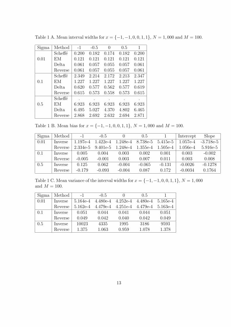
Table 1 A. Mean interval widths for x = {−1,−1, 0, 0, 1, 1}, N = 1, 000 and M = 100.

Sigma Method -1 -0.5 0 0.5 1Scheffe 0.200 0.182 0.174 0.182 0.200

0.01 EM 0.121 0.121 0.121 0.121 0.121Delta 0.061 0.057 0.055 0.057 0.061Reverse 0.061 0.057 0.055 0.057 0.061Scheffe 2.349 2.214 2.172 2.213 2.347

0.1 EM 1.227 1.227 1.227 1.227 1.227Delta 0.620 0.577 0.562 0.577 0.619Reverse 0.615 0.573 0.558 0.573 0.615Scheffe . . . . .

0.5 EM 6.923 6.923 6.923 6.923 6.923Delta 6.495 5.027 4.370 4.802 6.465Reverse 2.868 2.692 2.632 2.694 2.871

Table 1 B. Mean bias for x = {−1,−1, 0, 0, 1, 1}, N = 1, 000 and M = 100.

Sigma Method -1 -0.5 0 0.5 1 Intercept Slope0.01 Inverse 1.197e-4 1.422e-4 1.248e-4 8.738e-5 5.415e-5 1.057e-4 -3.718e-5

Reverse 2.334e-5 9.401e-5 1.248e-4 1.355e-4 1.505e-4 1.056e-4 5.916e-50.1 Inverse 0.005 0.004 0.003 0.002 0.001 0.003 -0.002

Reverse -0.005 -0.001 0.003 0.007 0.011 0.003 0.0080.5 Inverse 0.125 0.062 -0.004 -0.065 -0.131 -0.0026 -0.1278

Reverse -0.179 -0.093 -0.004 0.087 0.172 -0.0034 0.1764

Table 1 C. Mean variance of the interval widths for x = {−1,−1, 0, 0, 1, 1}, N = 1, 000and M = 100.

Sigma Method -1 -0.5 0 0.5 10.01 Inverse 5.164e-4 4.480e-4 4.252e-4 4.480e-4 5.165e-4

Reverse 5.162e-4 4.479e-4 4.251e-4 4.479e-4 5.163e-40.1 Inverse 0.051 0.044 0.041 0.044 0.051

Reverse 0.049 0.042 0.040 0.042 0.0490.5 Inverse 10023 4335 1995 3186 9593

Reverse 1.375 1.063 0.959 1.078 1.378

13

Table 1 D. Capture probabilities for x = {−1,−1, 0, 0, 1, 1}, N = 1, 000 and M = 100.




0.5 EM 0.993 0.995 0.996 0.995 0.994Delta 0.952 0.961 0.966 0.963 0.956Reverse 0.954 0.959 0.962 0.962 0.958

Table 2 A. Mean interval widths for x = {−1, 0, 0, 0, 0, 1}, N = 1, 000 and M = 100.




0.5 EM 7.658 7.658 7.658 7.658 7.658Delta 16.926 11.057 9.572 13.165 20.347Reverse 2.782 2.526 2.434 2.522 2.772

Table 2 B. Mean bias for x = {−1, 0, 0, 0, 0, 1}, N = 1, 000 and M = 100.

Sigma Method -1 -0.5 0 0.5 1 Intercept Slope0.01 Inverse 3.697e-4 1.244e-4 -6.728e-5 -3.166e-4 -5.785e-4 -9.366e-5 -4.675e-4

Reverse 1.689e-4 2.401e-5 -6.730e-5 -2.163e-4 -3.777e-4 -9.368e-5 -2.667e-40.1 Inverse 0.009 0.003 0.001 -0.003 -0.008 4.000e-4 -0.008

Reverse -0.012 -0.007 0.001 0.007 0.013 4.000e-4 0.01280.5 Inverse 0.223 0.112 -0.008 -0.116 -0.228 -0.0034 -0.226

Reverse -0.316 -0.156 0.004 0.166 0.327 0.005 0.3216

14

Table 2 C. Mean variance of the interval widths for x = {−1, 0, 0, 0, 0, 1}, N = 1, 000and M = 100.



Reverse 0.063 0.048 0.043 0.048 0.0630.5 Inverse 1.703e5 6.515e4 4.697e4 1.100e5 2.590e5

Reverse 1.314 0.898 0.752 0.904 1.325

Table 3 A. Mean interval widths for x = {−1,−1,−1, 1, 1, 1}, N = 1, 000, and M =100.




0.5 EM 6.385 6.385 6.385 6.385 6.385Delta 3.240 3.060 2.994 3.053 3.228Reverse 2.841 2.715 2.670 2.710 2.831

Table 3 B. Mean bias for x = {−1,−1,−1, 1, 1, 1}, N = 1, 000 and M = 100.

Sigma Method -1 -0.5 0 0.5 1 Intercept Slope0.01 Inverse 2.988e-4 1.640e-4 -1.020e-6 -1.070e-4 -2.281e-4 2.534e-5 -2.650e-4

Reverse 2.330e-4 1.311e-4 -1.018e-6 -7.414e-5 -1.623e-4 2.533e-5 -1.992e-40.1 Inverse 6.408e-4 -4.455e-4 -8.823e-4 -0.003 -0.004 -1.537e-3 -2.367e-3

Reverse -0.006 -0.004 -8.814e-4 7.777e-4 0.003 -1.421e-3 4.556e-30.5 Inverse 0.048 0.029 -0.012 -0.006 -0.024 0.007 -0.036

Reverse -0.118 -0.054 -0.010 0.074 0.138 0.006 0.128

15

Table 3 C. Mean variance of the interval widths for x = {−1,−1,−1, 1, 1, 1}, N =1, 000 and M = 100.



Reverse 0.051 0.046 0.045 0.046 0.0510.5 Inverse 2.784 2.175 1.960 2.163 2.781

Reverse 1.224 1.047 0.981 1.033 1.196

Table 4 A. Mean interval widths for x = {−1, 1} with 5 replicates at each point,N = 1, 000, and M = 100.




0.5 EM 4.269 4.269 4.269 4.269 4.269Delta 2.489 2.407 2.379 2.409 2.494Reverse 2.220 2.160 2.140 2.161 2.223

Table 4 B. Mean bias for x = {−1, 1} with 5 replicates at each point, N = 1, 000 andM = 100.

Sigma Method -1 -0.5 0 0.5 1 Intercept Slope0.01 Inverse -6.943e-5 -1.050e-4 -1.211e-4 -3.010e-5 1.145e-5 -6.284e-5 4.733e-5

Reverse -1.509e-4 -1.457e-4 -1.210e-4 1.063e-5 9.292e-5 -6.281e-5 1.288e-40.1 Inverse 0.001 2.540e-4 4.547e-4 -7.550e-4 -8.652e-5 1.734 -6.364e-4

Reverse -0.007 -0.004 4.410e-4 0.003 0.007 -1.118e-4 0.0070.5 Inverse 0.012 0.004 -0.007 -0.019 -0.030 -0.008 0.021

Reverse -0.157 -0.080 -0.005 0.069 0.144 -0.006 0.150

16

Table 4 C. Mean variance of the interval widths for x = {−1, 1} with 5 replicates ateach point, N = 1, 000 and M = 100.

Sigma Method -1 -0.5 0 0.5 10.01 Inverse 0.313 0.282 0.272 0.284 0.318

Reverse 0.205 0.189 0.184 0.190 0.2080.1 Inverse 0.015 0.014 0.013 0.014 0.014

Reverse 0.014 0.013 0.013 0.013 0.0140.5 Inverse 0.594 0.524 0.503 0.530 0.608

Reverse 0.303 0.278 0.270 0.280 0.308

Table 5 A. Mean interval widths for x = {−1, 1} with 10 replicates at each point,N = 1, 000, and M = 100.




0.5 EM 3.281 3.281 3.281 3.281 3.281Delta 2.235 2.195 2.181 2.194 2.235Reverse 1.983 1.955 1.945 1.955 1.983

Table 5 B. Mean bias for x = {−1, 1} with 10 replicates at each point, N = 1, 000and M = 100.

Sigma Method -1 -0.5 0 0.5 1 Intercept Slope0.01 Inverse 1.365e-4 9.139e-5 1.051e-4 4.927e-5 4.111e-5 8.467e-5 -4.658e-5

Reverse 4.480e-5 4.555e-5 1.051e-4 9.511e-5 1.328e-4 8.467e-5 1.080e-50.1 Inverse 0.001 9.699e-4 8.257e-4 3.806e-4 3.063e-5 6.414e-4 -5.056e-4

Reverse -0.008 -0.004 8.200e-4 0.005 0.009 5.640e-4 0.0090.5 Inverse 0.015 0.011 -3.283e-4 -0.004 -0.013 0.002 -0.014

Reverse -0.180 -0.087 -4.835e-4 0.092 0.181 0.001 0.180

17

Table 5 C. Mean variance of the interval widths for x = {−1, 1} with 10 replicates ateach point, N = 1, 000 and M = 100.


Reverse 5.579e-5 5.389e-5 5.326e-5 5.389e-5 5.580e-50.1 Inverse 5.365e-3 5.176e-3 5.114e-3 5.179e-3 5.369e-3


Reverse 0.118 0.112 0.110 0.112 0.117

Table 6 A. Mean interval widths for x = {−1,−1, 0, 0, 1, 1}, N = 100, 000 and M = 1.




0.5 EM 6.741 6.741 6.741 6.741 6.741Delta 9.029 12.018 10.734 16.613 22.927Reverse 2.881 2.706 2.644 2.705 2.880

Table 6 B. Mean bias for x = {−1,−1, 0, 0, 1, 1}, N = 100, 000 and M = 1.

Sigma Method -1 -0.5 0 0.5 1 Intercept Slope0.01 Inverse 6.767e-5 6.382e-5 6.398e-6 3.003e-5 -4.129e-5 2.533e-5 -5.034e-5

Reverse -3.270e-5 1.363e-5 6.392e-6 8.020e-5 5.906e-5 2.446e-5 5.174e-50.1 Inverse 0.002 5.279e-4 -2.070e-4 -0.001 -0.003 -3.358e-4 -2.306e-4

Reverse -0.008 -0.004 -2.007e-4 0.004 0.007 -2.401e-4 0.0080.5 Inverse 0.088 0.038 -1.064e-4 -0.051 -0.095 -0.004 -0.091

Reverse -0.173 -0.085 0.004 0.087 0.176 0.002 0.174

18

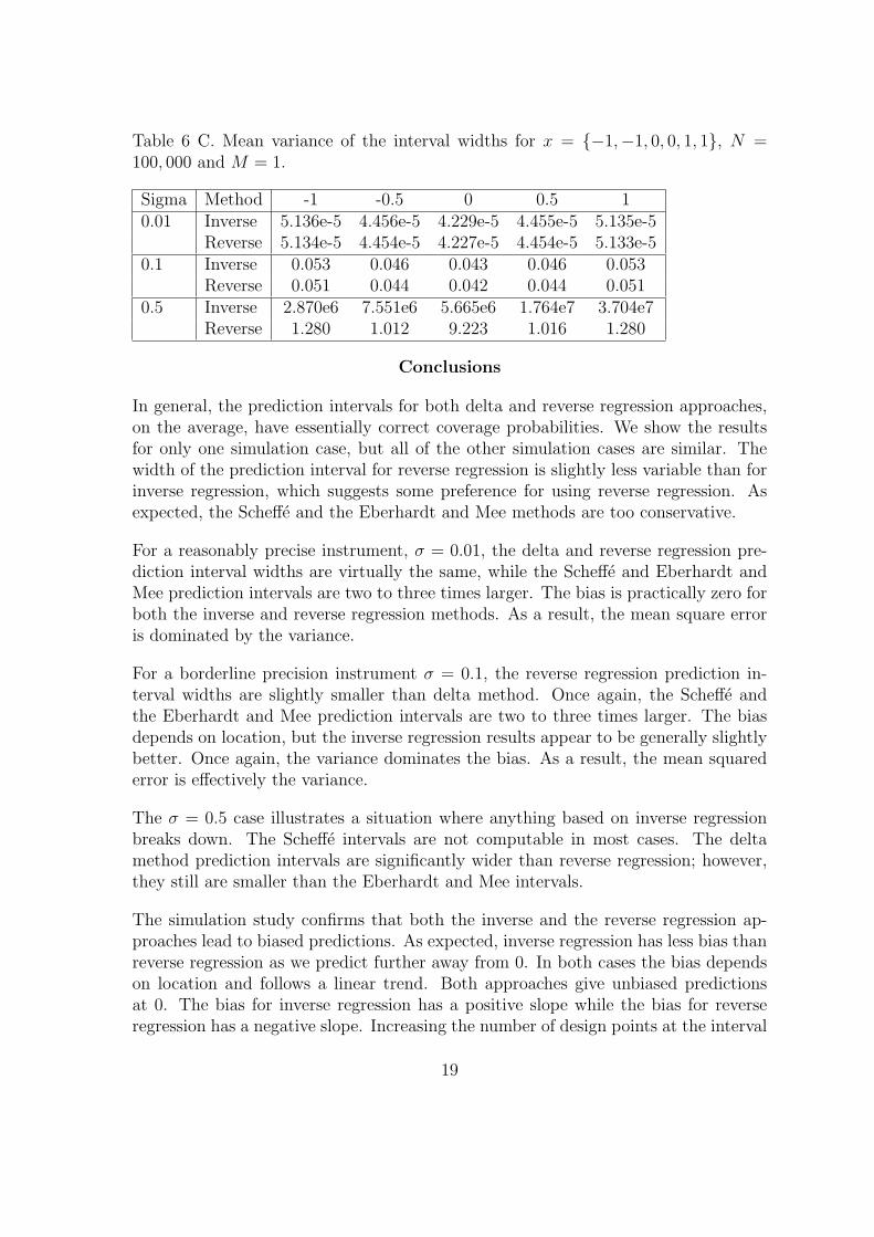
Table 6 C. Mean variance of the interval widths for x = {−1,−1, 0, 0, 1, 1}, N =100, 000 and M = 1.



Reverse 0.051 0.044 0.042 0.044 0.0510.5 Inverse 2.870e6 7.551e6 5.665e6 1.764e7 3.704e7

Reverse 1.280 1.012 9.223 1.016 1.280

Conclusions

In general, the prediction intervals for both delta and reverse regression approaches,on the average, have essentially correct coverage probabilities. We show the resultsfor only one simulation case, but all of the other simulation cases are similar. Thewidth of the prediction interval for reverse regression is slightly less variable than forinverse regression, which suggests some preference for using reverse regression. Asexpected, the Scheffe and the Eberhardt and Mee methods are too conservative.

For a reasonably precise instrument, σ = 0.01, the delta and reverse regression pre-diction interval widths are virtually the same, while the Scheffe and Eberhardt andMee prediction intervals are two to three times larger. The bias is practically zero forboth the inverse and reverse regression methods. As a result, the mean square erroris dominated by the variance.

For a borderline precision instrument σ = 0.1, the reverse regression prediction in-terval widths are slightly smaller than delta method. Once again, the Scheffe andthe Eberhardt and Mee prediction intervals are two to three times larger. The biasdepends on location, but the inverse regression results appear to be generally slightlybetter. Once again, the variance dominates the bias. As a result, the mean squarederror is effectively the variance.

The σ = 0.5 case illustrates a situation where anything based on inverse regressionbreaks down. The Scheffe intervals are not computable in most cases. The deltamethod prediction intervals are significantly wider than reverse regression; however,they still are smaller than the Eberhardt and Mee intervals.

The simulation study confirms that both the inverse and the reverse regression ap-proaches lead to biased predictions. As expected, inverse regression has less bias thanreverse regression as we predict further away from 0. In both cases the bias dependson location and follows a linear trend. Both approaches give unbiased predictionsat 0. The bias for inverse regression has a positive slope while the bias for reverseregression has a negative slope. Increasing the number of design points at the interval

19

boundaries decreases the bias for inverse regression; however, it has no effect on thebias for reverse regression. In general, inverse regression tends to be less biased thanreverse regression. The one case where forward regression appears to have less bias isthe rather unrealistic situation with only two points on the interval boundaries andmany points at the interval center. Such a situation does provide good ability to testfor lack-of-fit, but it fails to estimate the basic relationship well.

The bottom-line conclusions are somewhat mixed. Reverse regression appears tohave a slight edge in terms of the width of the prediction intervals for reasonableand borderline instruments. On the other hand, inverse regression appears to have adefinite edge in terms of bias for calibration experiments that replicate the intervalboundaries.

It is important to note that this study only considers a simple linear relationship.Future research intends to study more complicated calibration relationships includingmore than one calibration factor and higher-order models.

References

Berkson, J. (1969). ”Estimation of a Linear Function for a Calibration Line; Consid-eration of a Recent Proposal,” Technometrics, 11, 649-660.

Casella, G. and Berger, R.L. (2002). Statistical Inference, 2nd ed., Duxbury, CA.

Eberhardt, K.R., and Mee, R.W. (1994). ”Constant-Width Calibration Intervals forLinear Regression,” Journal of Quality Technology, 26, 21-29.

Graybill, F. (1976). Theory and Application of the Linear Model, Duxbury, NorthScituate, MA.

Halperin, M. (1970). ”On Inverse Estimation in Linear Regression,” Technometrics,12, 727-736.

Krutchkoff, R.G. (1967). ”Classical and Inverse Regression Methods of Calibration,”Technometrics, 9, 425-439.

Krutchkoff, R.G. (1969). ”Classical and Inverse Regression Methods of Calibrationin Extrapolation,” Technometrics, 11, 605-608.

Pham-Gia, T., Turkkan, N., and Marchand, E. (2006). ”Density of the Ratio of TwoNormal Random Variables and Applications,” Communications in Statistics - Theoryand Methods, 35, 1569-1591.

Scheffe, H. (1973). ”A Statistical Theory of Calibration,” The Annals of Statistics,1, 1-37.

20

Seber, G.A.F. (1977). Linear Regression Analysis, Wiley, NY.

Shalabh. (2001). ”Least Squares Estimators in Measurement Error Models underthe Balanced Loss Function,” Sociedad de Estadistica e Investigacion Operativa, 10,301-308.

Srivastava, A.K., and Shalabh. (1997). ”Asymptotic Efficiency Properties of Leastsquares in an Ultrastructural Model,” Sociedad de Estadistica e Investigacion Oper-ativa, 6, 419-431.

Williams, E.J. (1969). ”A Note on Regression Methods in Calibration,” Technomet-rics, 11, 189-192.

21

the prediction properties of inverse and reverse ... · the prediction properties of inverse and...

Documents