the problem of normalization and a normalized …...transactions on case-based reasoning vol. 4, no...

Transactions on Case-Based Reasoning Vol. 4, No 1 (2011) 3-17 ©2011, ibai-publishing, ISSN: 1867-366X , ISBN: 978-3-942952-09-5,

The Problem of Normalization and a Normalized Similarity Measure by Online Data

Anja Attig and Petra Perner

Institute of Computer Vision and Applied Computer Sciences, IBaI Kohlenstr. 2, 04107 Leipzig, Germany

[email protected], www.ibai-institut.de

Abstract. Case-based reasoning, image or data retrieval is based on similarity determination between the actual case and the cases in a database. It is preferable to normalize the similarity values between 0 and 1 in order to be able to compare different similarity values based on a scale. Similarity is thus imparted with a semantic meaning. The main problem arises when the case base is not yet complete and contains only a small number of cases while the other cases are collected incrementally as soon as they arrive in the system. In this case the upper and lower bounds of the feature values cannot be estimated close to the real values. This paper concerns possible methods for predicting the upper and lower bounds of a feature value and the problems that arise when these values are not correctly estimated due to a limited number of samples or a parameter distribution that is not available a-priori. The aim is to develop a method for learning the upper and the lower bounds of a feature value and to develop a methodology for dealing with change in semantic meaning of the similarity.

1 Introduction

Case-based reasoning, image or data retrieval is based on similarity determination between the actual case and the cases in a database. It is preferable to normalize the similarity values between 0 and 1 in order to be able to compare different similarity values based on a scale. A scale between 0 and 1 gives us a symbolic understanding of the meaning of the similarity value. The value of 0 indicates identity of the two cases while the value of 1 indicates the cases are unequal. On the scale of 0 and 1

4 Anja Attig and Petra Perner

the value of 0.5 means neutral and values between 0.5 and 0 mean more similarity and values between 0.5 and 1 mean more dissimilarity

Different normalization procedures are known. The most popular one is the normalization to the upper and lower bounds of a feature value.

The main problem arises when the case base is not yet completely filled and contains only a small number of cases while the other cases are collected incrementally as soon as they arrive in the system. In this case the upper and lower bounds of a feature value min, , max, ,,i k i kx x� �� can only be judged based on this limited

set of cases at the point in time kt and must not meet the true values of ixmin, and

ixmax, of feature i. Then the scale of similarity might change over time periods ktwhich will lead to different decisions for two cases at the points in time kt and lkt � .

This paper describes the problem of normalization in an incremental case-based learning system.

This paper deals with possible methods for predicting the upper and lower bounds of a feature value and the problems that arise when these values are not correctly estimated due to a limited number of samples or information that is not available a-priori .

The aim is to develop a method for learning ixmin, and ixmax, of a feature i and a methodology for dealing with change in the semantic meaning of Sim .

In Section 2, we describe related work while in Section 3 we describe the normalization problem based on an upper and a lower value for the feature. The experimental set-up is described in Section 4 and the results are presented in Section 5. The results are discussed in Section 6 and finally conclusions are set forth in Section 7.

2 Related Work

The determination of similarity between cases is one of the key concepts in CBR [1]. Several studies on similarity have been done for this purposes. Learning of similarity measures has been introduced by Richter [2] as an outcome of the PATDEX project, where the weights and the features are updated based on the feedback of the user. Xiong and Funk studied the building of similarity by using learning strategies such as relevance feedback [3] and memetic algorithm [4]. Strategies for feature weighting to learn the similarity have been introducted by Wettschereck and Aha [5], Little et. al [6], Ahn et. al [7] and Bichindaritz [8][9]. Jarmulak et. al [8] used genetic algorithm to update the feature weights. Lerning similarity function by qualitative feedback has been studied by Cheng and Hullermeier [9]. Transforming similarity into a linear space of feature combination has been studied by L. Bobrowski, M. Topczewska [12]. Graph similarity and learning of graph similarity has been studied by Perner [13]. In all these studies plays normalization not a central role. The parameters for normalization and the kind of normalization are just given a-priori.

A First Note on the Problem of Normalization 5

However, studies in data mining show that normalization has a big impact on the final results [14, 15].Normalization allows comparing different experiments based on the same application independent from the scale of the features. Normalization is a necessary step in many applications. Well known normalization procedures are the min/max normalization, the z-transformation, the log transformation, and the rank transformation [15, 16].

For the min/max normalization we need to know the upper and lower bounds of the feature value. In case of a technical system the values might be judged by looking at the systems characteristic [16, 17] or by calculating the system transfer function. Other applications rely on the perceptual observation for the application [18]. However, in most of today’s applications this is not applicable, in particular when the data arrive in temporal sequence.

The other transformations require knowledge of the probability distribution of the application. If a large enough set of data is available, the probability distribution can be estimated from the data. This is the parametric method.

The situation is tricky if we are dealing with online applications where we want to start with a small set of data that increases over time and we need to develop incremental methods for normalization.

In our study we investigated what the problem with normalization is in CBR. A study in that direction has not been done before in CBR although the method of normalization and the method of parameter setting has a big impact on the performance of the CBR system. With our study we like to direct the intention of the researchers to this problem and give a first idea how to deal with it.

3 The Problem of Normalization and Similarity

Suppose we have a data set of n-features. Each feature of the data set obeys a distribution (see Fig.1), this can be any distribution. In case of Fig. 1 we chose the normal distribution.

Fig. 1. Distribution of one feature and parameters of the distribution


We can define a tolerance range iT for each feature i that gives us an upper bound

ixmax, and a lower bound ixmin, for the values of the feature i . The tolerance range should be determined in such a way that the number of samples that are outside the tolerance range is low. The error rate ixp , is the number of non-classified case inonN ,

to all cases N :

NN

p inonix

,, � (1)

The error rate of the feature i is equal to the marked area under the probability density function in Figure 1:

, ( )x i i ip P x T� � (2)

, min, max,x i i i i ip P x T x T� �� (3)

which is

, min, max,( )x i i i i ip P x T P x T� � � (4)

The error rate should decrease the larger iT becomes (see Figure 2). However, iTshould not be chosen too large. Feature values that do not appear frequently should not be taken into account and should be considered an outlier.

px,i

Ti

Fig. 2. Error rate ,x ip in relation to tolerance range iT

We can observe the error rate and adjust iT when the error rate exceeds a predefined threshold as the classifier has evaluated k samples.

Another important parameter that has to be observed is the similarity value. The similarity between two cases x and y is calculated as follows:

� ��i

jjii yx

nyxSim

1

))((1),( (5)


with 1j � the city-block-metric, x� and y� the normalized feature of x and y.

Let y be cases that are not classified and lx the classified cases. The classification rule based on all features for a similarity-based classification can be:

),(min l

xxySimSim

l�� (6)

in case of the nearest-neighbor rule and

( , )lSim y x K� (7)

in case of the semantic similarity rule with K the threshold for similarity. The error rate of the classifier is cp that is defined as the number of misclassified

case misN to the number of all cases N

misc

Np

N� (8)

If the similarity value is not between 0 and 1 (see Figure 3), we normalize the similarity measure by the upper and the lower bounds of the feature value.

0 0.5 1similar neutral dissimilar

more or less less or moresimilar dissimilar

Fig. 3. Similarity values, scale and semantic meaning

This gives us a semantic understanding of similarity. Identity of two cases results in the similarity value of 0 and dissimilarity of two cases results in the similarity value of 1. Between the values 0 and 0.5 the cases are more or less similar; between 0.5 and 1 the cases are more or less dissimilar (see Fig. 3).

The difference in similarity

, ,x y x zSim Sim Sim� � � (9)

allows us to judge the similarity relation between different cases x, y and z, andshould reflect the real distance between the cases and, as such, provide us with a semantic understanding of the similarity.

The difference between two cases x and y can be observed over time. The change of the similarity between times kt and lt can be calculated:

),(),(),,( , yxSimyxSimttyxSimlk ttlk �� (10)


For the points in time kt and lt , we can calculate the mean change of similarity and the maximum change of similarity for the cases of a data set. Depending on the outcome, further actions have to be taken.

If the values of min.ix and max,ix are chosen too low or too large and do not come close to the real values, then the scale behind Sim may not be correct and misclassification may occur. In the worst case, two cases that are similar may be judged dissimilar since the value of Sim is over 0.5.

If we know the probability density distribution of a feature i; we can judge the parameters min,ix and max,ix according to Dreyer and Sauer [19].

If we do not know a-priori the distribution and if the data are collected incrementally, then we cannot judge these parameters in advance. The normalization and the scale for similarity will become a problem. We will set forth in the following Section the problems that arise when we normalize to min,ix and max,ix and how we can deal with the problems in case of an incremental case-based learning system.

4 Experiment

In the following we want to demonstrate how the classifier behaves if we do not know the right values for the upper and lower bounds at different points in time. The experiment is done based on the iris data set. The data set has four features and 150 data. The data are grouped in to three classes.

We observe the development of the error rate for each feature depending on 5 different data sets 1N … 5N .

The following tests have been carried out:

1. Development of the error rate ,x ipFor the data set 1N we choose randomly five data from each class from the iris data set. For data set 2N we choose again five data from each class and add this data to data set 1N . Analogously, we choose for 3N ten data from each class and for

4N and 5N fifteen data from each class. Note that the same data can be used in two or more data sets.

For each data set kN and for each feature i, we calculate min, ,i kx and max, ,i kx .

Then we compute , max, , min, ,i k i k i kT x x� � for each feature i.

Furthermore, let kT� be the set },,,,{~,,,1 knkikk TTTT �� .

For the data sets kN and 1 \k kx N N�� we check for each feature i if

min, , max, ,i k i i kx x x� � or not. Then we can calculate , ,x i kp


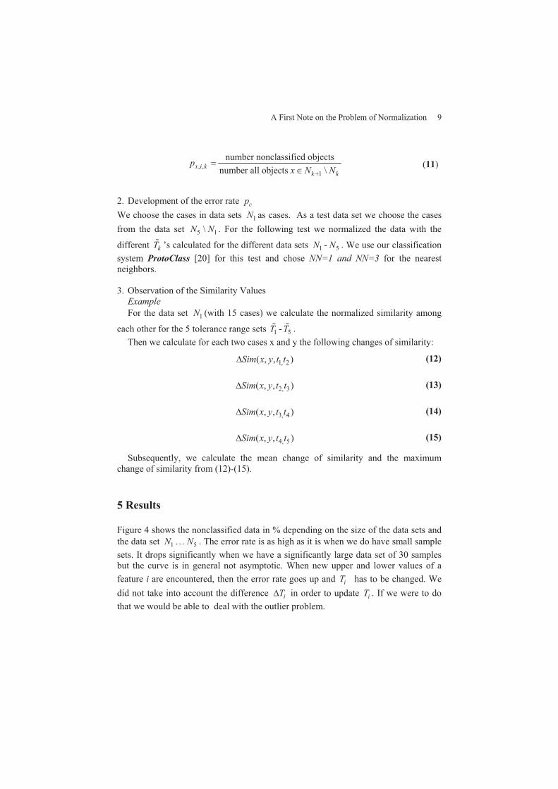
, ,1

number nonclassified objectsnumber all objects \x i k

k kp

x N N��

�(11)

2. Development of the error rate cpWe choose the cases in data sets 1N as cases. As a test data set we choose the cases from the data set 5 1\N N . For the following test we normalized the data with the

different kT� ’s calculated for the different data sets 1N - 5N . We use our classification system ProtoClass [20] for this test and chose NN=1 and NN=3 for the nearest neighbors.

3. Observation of the Similarity Values ExampleFor the data set 1N (with 15 cases) we calculate the normalized similarity among

each other for the 5 tolerance range sets 1T� - 5T� .Then we calculate for each two cases x and y the following changes of similarity:

1, 2( , , )Sim x y t t� (12)

2, 3( , , )Sim x y t t� (13)

3, 4( , , )Sim x y t t� (14)

4, 5( , , )Sim x y t t� (15)

Subsequently, we calculate the mean change of similarity and the maximum change of similarity from (12)-(15).

5 Results

Figure 4 shows the nonclassified data in % depending on the size of the data sets and the data set 1N … 5N . The error rate is as high as it is when we do have small sample sets. It drops significantly when we have a significantly large data set of 30 samples but the curve is in general not asymptotic. When new upper and lower values of a feature i are encountered, then the error rate goes up and iT has to be changed. We did not take into account the difference iT� in order to update iT . If we were to do that we would be able to deal with the outlier problem.


Fig. 4. Error rate ,x ip versus sample number Fig. 5. Error rate ,x ip versus sample sets 1 4...N N

Fig. 6. Tolerance range ,i kT versus sample number

Fig. 7. Tolerance range ,i kT versus sample

sets 1 5...N N

Fig. 8. Error rate ,x ip versus ,i kT for all four different features


Figure 6 shows that ,i kT increase as more data are arriving and that, after some time, it goes into saturation. Figure 8 shows the nonclassified data in % depending on

,i kT . Small changes of ,i kT causes large changes of the error rate.

05

101520253035404550

withoutnormalisation

correct

not classified

wronglyclassified

Fig. 9. Error rate cp versus tolerance range 1T� … 5T� for 1NN �

05

101520253035404550

withoutnormalisation

correct

not classified

wronglyclassified

Fig. 10. Error rate cp versus tolerance range 1T� … 5T� for 3NN �

The nonclassified data decreases the more ,i kT converges toward the correct iT(see Figure 9 for NN=1 and Figure 10 for NN=3). In this example the wrongly classified data are always the same. This might be different in other experiments but at least it shows that the wrong classification is not the main problem. The problem is that some samples cannot be classified and case-based maintenance [21] has to be started. The classification is done based on the nearest neighbor principle. The semantic scale does not play a significant role in this situation. If we look for the changes in the similarity value, it is apparent that the similarity value changes


significantly. Figure 11 shows for some samples the pair-wise similarity value for different kT� . The samples become more similar as ,i kT becomes larges and as ,i kTconverges more toward the real iT .

The mean in similarity range is from 0.07 to 0.0 (see Figure 12). The max similarity value range is from 0.2 to 0.0. This means that the semantic of the similarity changes drastically. Samples that are more dissimilar become more similar after ,i kT converges toward the real iT s.

Fig. 11. Pair-wise similarity for three cases depending on several cases

Fig. 12. Mean and maximal similarity difference for four different points in time


6 Discussion

Normalization of the similarity measure by the lower and upper bounds of the features i allow us to compare different samples on a scale between 0 and 1. The similarity is thus imparted with a semantic meaning and allows a human to better grasp the similarity.

This semantic is only true if the values used for normalization are true. If we normalize to a lower and an upper bound of the features i, then ixmin, and

ixmax, must be true values. If we only use the nearest neighbor rule then classification is done based on the nearest distance. The semantic scale plays no role. We are then only faced with the problem that samples cannot be classified because of wrong lower and upper bounds. Depending on how large an error rate we allow for each feature, we have to change the lower and upper bounds after some time.

A case-based reasoning system has to monitor the lower and upper bounds for the feature value of each feature and start case-based maintenance when the error rate

,x ip exceeds a threshold. The system should keep the frequency histogram for each feature in memory and update this histogram incrementally until a probability density distribution can be estimated from the histogram.

If we rely on the semantics of the similarity helping a human to judge the similarity between two samples, we are faced with the problem of wrong classification and with the problem of wrong semantic. Two cases that might have been more dissimilar might become more similar after some time. If these two cases are judged based on the semantic rule, they might be wrongly classified in the end.

This means that, as long as iT has not reached the true values, the semantic similarity rule should not be used for classification or the semantic similarity should not be shown for comparison purposes. It is better to rely on the nearest neighbor principle.

7 Conclusion

Normalization allows us to compare different cases on a scale from 0 to 1 andprovides us with a semantic understanding of similarity. The value of 0 means identity and the value of 1 means dissimilar. In between, the value of 0.5 means neutral while the values on a scale from 0.5 to 0 mean more similar and the values from 1 to 0.5 mean more dissimilar.

The problem of normalization has not been studied in CBR yet under the aspect of different normalization methods and the methods for parameter setting. The situation is tricky if we are dealing with online applications where we want to start with a small set of data that increases over time and we need to develop incremental methods for normalization.

In our study we investigated what the problem with normalization is in CBR. A study in that direction has not been done before in CBR although the method of


normalization and the method of parameter setting has a big impact on the performance of the CBR system. With our study we like to direct the intention of the researchers to this problem and give a first idea how to deal with it.

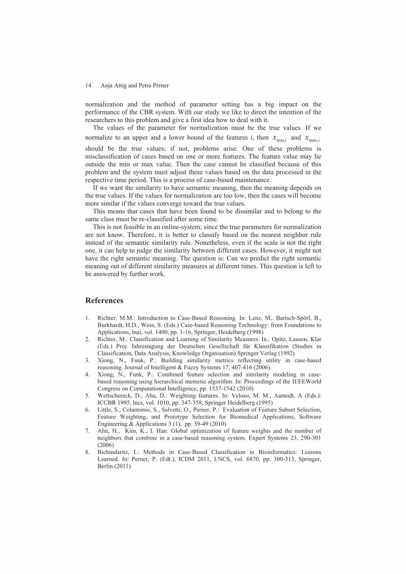
The values of the parameter for normalization must be the true values. If we normalize to an upper and a lower bound of the features i, then ixmin, and ixmax,

should be the true values; if not, problems arise. One of these problems is misclassification of cases based on one or more features. The feature value may lie outside the min or max value. Then the case cannot be classified because of this problem and the system must adjust these values based on the data processed in the respective time period. This is a process of case-based maintenance.

If we want the similarity to have semantic meaning, then the meaning depends on the true values. If the values for normalization are too low, then the cases will become more similar if the values converge toward the true values.

This means that cases that have been found to be dissimilar and to belong to the same class must be re-classified after some time.

This is not feasible in an online-system; since the true parameters for normalization are not know. Therefore, it is better to classify based on the nearest neighbor rule instead of the semantic similarity rule. Nonetheless, even if the scale is not the right one, it can help to judge the similarity between different cases. However, it might not have the right semantic meaning. The question is: Can we predict the right semantic meaning out of different similarity measures at different times. This question is left to be answered by further work.

References

1. Richter, M.M.: Introduction to Case-Based Reasoning. In: Lenz, M,. Bartsch-Spörl, B., Burkhardt, H.D., Wess, S. (Eds.) Case-based Reasoning Technology: from Foundations to Applications, lnai, vol. 1400, pp. 1-16, Springer, Heidelberg (1998)

2. Richter, M.: Classification and Learning of Similarity Measures. In.: Opitz, Lausen, Klar (Eds.) Proc Jahrestagung der Deutschen Gesellschaft für Klassifikation (Studies in Classification, Data Analysis, Knowledge Organisation) Springer Verlag (1992)

3. Xiong, N., Funk, P.: Building similarity metrics reflecting utility in case-based reasoning. Journal of Intelligent & Fuzzy Systems 17, 407-416 (2006).

4. Xiong, N., Funk, P.: Combined feature selection and similarity modeling in case- based reasoning using hierarchical memetic algorithm. In: Proceedings of the IEEEWorld Congress on Computational Intelligence, pp. 1537-1542 (2010)

5. Wettschereck, D., Aha, D.: Weighting features. In: Veloso, M. M., Aamodt, A (Eds.): ICCBR 1995, lncs, vol. 1010, pp. 347-358, Springer Heidelberg (1995)

6. Little, S., Colantonio, S., Salvetti, O., Perner, P.: Evaluation of Feature Subset Selection, Feature Weighting, and Prototype Selection for Biomedical Applications, Software Engineering & Applications 3 (1), pp. 39-49 (2010)

7. Ahn, H., Kim, K., I. Han: Global optimization of feature weights and the number of neighbors that combine in a case-based reasoning system. Expert Systems 23, 290-301 (2006)

8. Bichindaritz, I.: Methods in Case-Based Classification in Bioinformatics: Lessons Learned. In: Perner, P. (Edt.), ICDM 2011, LNCS, vol. 6870, pp. 300-313, Springer, Berlin (2011)


9. Bichindaritz I.: Comparison of Reuse Strategies for Case-Based Classification in Bioinformatics. In: Wiratunga, N., Ram, A. (Eds.) ICCBR 2011, lncs, vol. 6880, pp. 393-407, Springer, Berlin (2011)

10. Jarmulak, J., Craw, S., Rowe, R.: Genetic algorithms to optimize CBR retrieval. In: Blanzieri, E., Portinale, L (Eds.) EWCBR 2000, lncs, vol. 1898, pp. 136-147, Springer, Heidelberg (2000)

11. Cheng, W., Hüllermeier, E.: Learning similarity functions from qualitative feedback In: Althoff, K.D., Bergmann, R., Minor, M., Hanft, A. (Eds.): ECCBR 2008. lncs, vol. 5239 pp. 120-134, Springer, Heildelberg (2008)

12. Bobrowski, L., Topczewska, M.: Improving the K-NN Classification with the Euclidean Distance Through Linear Data Transformations. In: Perner, P. (Ed.): ICDM 2004, lncs, vol. 3275, pp. 23-32, Springer, Heidelberg (2004)

13. Perner P.: Case-Based Reasoning for Image Analysis and Interpretation, In: Chen, C., Wang, P.S.P.: Handbook on Pattern Recognition and Computer Vision, 3rd Edition, pp. 95-114, World Scientific Publisher (2005)

14. Fayyad, U.M., Piatesky-Shapiro G., Smyth P, Utuhrusamy, R.: Advance in Knowledge Discovery and Data Mining, AAAI Press (1996)

15. Perner, J.: Characterizing Cell Types through Differentially Expressed Gene Clusters Using a Model-based Approach, ibai-publishing, Fockendorf, ISBN 978-3-942952-01-9 (2011)

16. Stolcke A., Kajarekar S., Ferrer L.: Nonparametric feature normalization for SVM-based speaker verification. In: IEEE International Conference on Acoustics, Speech and Signal Processing, ICASSP 2008, pp. 1577 – 1580 (2008)

17. Molau S., Pitz M., Ney, H.: Histogram based normalization in the acoustic feature space, 2. IEEE Workshop on Automatic Speech Recognition and Understanding, pp. 21-24 (2001)

18. Pisoni, D.B.: Long-term memory in speech perception: Some new findings on talker variability, speaking rate and perceptual learning. Speech Communication 13 (1-2) October, 109-125 (1993)

19. Dreyer, H., Sauer, W.: Prozeßanalyse, Verlag Technik, Berlin (1982) 20. Perner, P.: Prototype-Based Classification. Applied Intelligence 28(3), 238-246 (2008) 21. Perner, P.: Case-base maintenance by conceptual clustering of graphs. Engineering

Applications of Artificial Intelligence. 19 (4), 381-295 (2006)


Appendix

SEPALLEN Iris 1N 2N 3N 4N 5N

kN 150 15 30 60 105 150

min, ,i kx 4,3 4,6 4,3 4,3 4,3 4,3

max, ,i kx 7,9 6,9 7,7 7,7 7,7 7,7

,i kT 3,6 2,3 3,4 3,4 3,4 3,4

,i k� 5,84335,8467

(Median:5,8000)

5,7333 5,7617 5,8429 5,8287

,i k� 0,8281 0,72198563 0,8401 0,8491 0,8866 0,8647

Number of nonclassified data

1 /k kx N N��-

4Setosa_14,Setosa_42,Setosa_43,Virginica_24

0 0 0 -

, ,x i kp - 4/15=0,27 0 0 0 -

SEPALWI Iris 1N 2N 3N 4N 5N

kN 150 15 30 60 105 150

min, ,i kx 2 2,7 2,2 2,2 2 2

max, ,i kx 4,4 4,4 4,4 4,4 4,4 4,4

,i kT 2,4 1,7 2,2 2,2 2,4 2,4

,i k� 3,0573 3,2600 (Median: 3,2000) 3,0233 3,0383 3,0410 3,0407

,i k� 0,4359 0,50448827 0,4967 0,4357 0,4415 0,4313


1 /k kx N N��-

6Setosa_42

Versicolor_04Versicolor_41Virginica_07Virginica_19Virginica_20

0 1Versicolor_11 0 -

, ,x i kp - 6/15=0,4 0 1/45=0,022 0 -


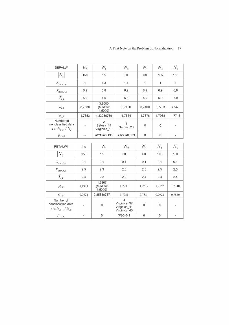
SEPALWI Iris 1N 2N 3N 4N 5N

kN 150 15 30 60 105 150

min, ,i kx 1 1,3 1,1 1 1 1

max, ,i kx 6,9 5,8 6,9 6,9 6,9 6,9

,i kT 5,9 4,5 5,8 5,9 5,9 5,9

,i k� 3,75803,8000

(Median:4,5000)

3,7400 3,7400 3,7733 3,7473

,i k� 1,7653 1,83056769 1,7884 1,7676 1,7968 1,7716 Number of

nonclassified data

1 /k kx N N��-

2Setosa_14

Virginica_19

1Setosa_23 0 0 -

, ,x i kp - =2/15=0,133 =1/30=0,033 0 0 -

PETALWI Iris 1N 2N 3N 4N 5N

kN 150 15 30 60 105 150

min, ,i kx 0,1 0,1 0,1 0,1 0,1 0,1

max, ,i kx 2,5 2,3 2,3 2,5 2,5 2,5

,i kT 2,4 2,2 2,2 2,4 2,4 2,4

,i k� 1,1993 1,2867

(Median:1,5000)

1,2233 1,2317 1,2152 1,2140

,i k� 0,7622 0,85880787 0,7981 0,7884 0,7922 0,7830


1 /k kx N N��- 0

3Virginica_37Virginica_41Virginica_45

0 0 -

, ,x i kp - 0 3/30=0,1 0 0 -

the problem of normalization and a normalized …...transactions on case-based reasoning vol. 4, no...

Documents