the pyrosetta interactive platform for protein structure...

The PyRosetta Interactive Platform for Protein Structure Prediction and Design

A Set of Educational Modules

Jeffrey J. Gray Sidhartha Chaudhury

Sergey Lyskov

Chemical & Biomolecular Engineering Program in Molecular Biophysics

Johns Hopkins University Baltimore, Maryland

i

Table of Contents Preface .......................................................................................................................................................... 1 Workshop #1: PyMol ..................................................................................................................................... 3 Suggested Readings .................................................................................................................................. 3 Basic Operations ....................................................................................................................................... 3 Structural Analysis ..................................................................................................................................... 4 Comparing Molecules ............................................................................................................................... 6 High‐Quality Visualization and Scripting ................................................................................................... 7

Workshop #2: PyRosetta ............................................................................................................................... 8 Basic Elements .......................................................................................................................................... 8 Basic Python .............................................................................................................................................. 8 Basic PyRosetta ......................................................................................................................................... 9 Protein geometry .................................................................................................................................... 10 Manipulating protein geometry .............................................................................................................. 11 Programming ........................................................................................................................................... 11 Programming exercises ........................................................................................................................... 12 References .............................................................................................................................................. 13

Workshop #3: PyRosetta Scoring ................................................................................................................ 14 Scoring Poses .......................................................................................................................................... 14 Programming exercises ........................................................................................................................... 16 References .............................................................................................................................................. 16

Workshop #4: PyRosetta Folding ................................................................................................................ 17 Suggested Readings ................................................................................................................................ 17 A simple de novo folding algorithm ........................................................................................................ 17 Low‐resolution (centroid) scoring ........................................................................................................... 18 Protein fragments ................................................................................................................................... 19 Programming exercises ........................................................................................................................... 20 Thought questions .................................................................................................................................. 20

Workshop #5: PyRosetta Refinement ......................................................................................................... 21 Suggested Reading .................................................................................................................................. 21 Small and shear moves ........................................................................................................................... 21 Minimization moves ................................................................................................................................ 22 Monte Carlo object ................................................................................................................................. 23 Trial Mover .............................................................................................................................................. 24 Sequence and Repeat Movers ................................................................................................................ 24 Refinement Protocol ............................................................................................................................... 25 Programming exercises ........................................................................................................................... 26 Thought questions .................................................................................................................................. 26

Workshop #6: Packing & Design ................................................................................................................. 27 Suggested readings ................................................................................................................................. 27 Side‐chain conformations, the rotamer library, and Dunbrack energies ............................................... 27 Monte Carlo side‐chain packing .............................................................................................................. 28 Packing for refinement ........................................................................................................................... 28 Design ...................................................................................................................................................... 29 Programming exercises ........................................................................................................................... 30 Thought questions .................................................................................................................................. 32

ii

References .............................................................................................................................................. 32 Workshop #7: Docking ................................................................................................................................ 33 Suggested Readings ................................................................................................................................ 33 Fast‐Fourier transform based docking via ZDOCK .................................................................................. 33 Docking moves in Rosetta ....................................................................................................................... 33 Low‐resolution docking via RosettaDock ................................................................................................ 35 Job distributor ......................................................................................................................................... 36 High‐resolution docking .......................................................................................................................... 37 Docking Funnel ........................................................................................................................................ 38 Conformer Selection for Ensemble Docking ........................................................................................... 38 Induced‐Fit Docking ................................................................................................................................ 39 Programming assignments ...................................................................................................................... 39

Workshop #8: Loop Modeling ..................................................................................................................... 40 Suggested Readings ................................................................................................................................ 40 Fold Tree ................................................................................................................................................. 40 Cyclic coordinate descent (CCD) loop closure ........................................................................................ 42 Multiple loops ......................................................................................................................................... 42 Loop building ........................................................................................................................................... 43 High‐resolution loop protocol ................................................................................................................. 43 Simultaneous loop modeling and docking .............................................................................................. 44

Coda ............................................................................................................................................................ 45 Appendix A: Command Reference .............................................................................................................. 46 Python Commands and Syntax ............................................................................................................... 46 Python Math ........................................................................................................................................... 46 Rosetta: Vector ....................................................................................................................................... 46 Rosetta: Pose Object ............................................................................................................................... 47 Rosetta: Scoring ...................................................................................................................................... 48 Rosetta Full‐atom Scoring Functions ...................................................................................................... 48 Residue Type Set Mover ......................................................................................................................... 49 MoveMap ................................................................................................................................................ 49 Fragment Movers .................................................................................................................................... 49 Small and Shear Movers.......................................................................................................................... 49 Minimize Mover ...................................................................................................................................... 50 MonteCarlo ............................................................................................................................................. 50 TrialMover ............................................................................................................................................... 50 SequenceMover and RepeatMover ........................................................................................................ 50 Side Chain Packing Movers ..................................................................................................................... 51 Fold Tree ................................................................................................................................................. 51 Rigid Body Movers .................................................................................................................................. 52 Docking Movers ...................................................................................................................................... 52 Loops ....................................................................................................................................................... 53 Job Distributor ......................................................................................................................................... 53

Appendix B: Residue Parameter Files ......................................................................................................... 54

1

Preface Structures of proteins and protein complexes help explain biomolecular function, and computational methods provide an inexpensive way to predict unknown structures, manipulate behavior, or design new proteins or functions. The protein structure prediction program Rosetta, developed by a consortium of laboratories in the Rosetta Commons, has an unmatched variety of functionalities and is one of the most accurate protein structure prediction and design approaches (Das & Baker, Ann Rev Biochem 2008; Gray, Curr Op Struct Biol 2006). To make the Rosetta approaches broadly accessible to biologists and biomolecular engineers with varied backgrounds, we developed PyRosetta, a Python-based interactive platform for accessing the objects and algorithms within the Rosetta protein structure prediction suite. In PyRosetta, users can measure and manipulate protein conformations, calculate energies in low- and high-resolution representations, fold proteins from sequence, model variable regions of proteins (loops), dock proteins or small molecules, and design protein sequences. Furthermore, with access to the primary Rosetta optimization objects, users can build custom protocols for operations tailored to particular biomolecular applications. Since the Python-based program can be run within the visualization software PyMol, search algorithms can be viewed on-screen in real time. In this book, we have compiled a set of workshops to teach both the fundamentals and the practical application of protein structure prediction and design. Workshops assume basic knowledge of protein structure and familiarity with computers, and readings and references are provided in each chapter for more in-depth study. Each workshop covers a single topic in the field and walks the reader through the basic operations in a one- to two-hour session. Interactive exercises are incorporated so that the reader gains hands-on experience using the variety of commands available in the toolkit. The text is arranged progressively, beginning with an introduction of the PyMol visualization package, proceeding through the fundamentals of protein structure and energetics, and then progressing through the applications of protein folding, refinement, packing, design, docking, and loop modeling. A set of tables is provided at the end of the book as a reference of the available commands. Additional resources on the Rosetta program are available online. The PyRosetta web site, pyrosetta.org, includes additional example and application scripts. A web-based user forum is in development and we hope that the PyRosetta community will share their experiences as well as useful scripts so that we build a repository of useful functions. For the expert, documentation on the underlying C++ code is available at www.rosettacommons.org under the TikiWiki application (www.rosettacommons.org/tiki/tiki-index.php). PyRosetta is built upon the Rosetta 3 platform, so objects available in PyRosetta will have the same underlying data structures and functionality. These modules were created at the Homewood campus of Johns Hopkins University over the course of two semesters, Spring 2008 and Spring 2009, for the Chemical & Biomolecular Engineering class “Computational Protein Structure Prediction and Design.” We acknowledge the contributions of the many developers of the Rosetta community (see www.rosettacommons.org) for their creation of the Rosetta protein structure prediction suite, upon which PyRosetta is built. Julian Rosenberg and J. D. Bagert, former students of the class before PyRosetta, pioneered early drafts of the workshops in 2008 through a Technology

2

Fellowship from the JHU Center for Educational Resources. We thank Richard Shingles of the Center for Educational Resources for assistance in the workshop conception and in the formal assessment. The National Institutes of Health supported J.J.G., S.C., and S.L. through grant numbers GM-078221 and GM-073151, and the National Science Foundation supported J.J.G. through CAREER award number 0846324. Finally, we thank the wonderful JHU students in both semesters for their help, feedback, patience, and fun times writing code in the lab.

To complete these modules, you will need:

1. PyMol – www.pymol.org 2. Python – www.python.org 3. iPython – ipython.scipy.org 4. PyRosetta – www.pyrosetta.org

All packages are free and available for Mac and Linux platforms. PyRosetta is for PC is under development and expected in December 2009.

3

Workshop #1: PyMol PyMol is a molecular visualization tool. There are many such tools available, both commercial and publicly available (SwissPDB, rasmol, VMD, MolSim, Insight II, etc.). PyMol is particularly attractive for us since it has excellent features for viewing, it is fast and the display quality is superb, it can handle multiple molecules at once and it is easy to define custom objects such as complexes or sets of atoms. It is also open-source and extensible, so the expert user can create new functions such as colors and measurements related to protein design specifications. The goals of this workshop are to have you become familiar with (1) the basic operation of the software, (2) the tools for analyzing protein structures and for creating high-quality pictures, and (3) the ability to create and save scripts for repeated use. Suggested Readings

1. Introductory: Chapters 1 and 2 of Brandon and Tooze, Introduction to Protein Structure, Garland Publishing (1999).

2. Advanced: J. S. Richardson, “The Anatomy and Taxonomy of Protein Structure,” 1981 (updated 2000-2007), available at http://kinemage.biochem.duke.edu/teaching/anatax.

Basic Operations

1. Download PDB file 1YY8.pdb from www.rcsb.org.

2. Open PyMol (if asked, use the PyMol + Tcl/Tk mode) and load the 1YY8 (from the menu bar at the top of the upper window, “File→Open→(select your file)”.

3. Use the mouse and mouse buttons to rotate, translate, and zoom the molecule.

On Linux or PC: Left button=rotate, middle button=translate, right button=zoom. On a Mac: click=rotate, alt/option+click=translate, control+click=zoom

4. The buttons at the top right can set the viewing parameters. A=Actions, H=Hide, S=Show, L=Label, C=Color. In the line for 1YY8, select “Hide→Everything”, then “Show→Cartoon”, then “Color→By Chain→By Chain (e,c)”, then “Label→Chains.”

5. You should see two copies of the antibody fragment, since there were two copies of the 6. antibody in the unit cell of the crystal which was measured to determine the structure.

You should be able to see two separate chains in each antibody fragment. If you click on any atom, the console window will display information identifying that atom. Confirm that the four chains are identified as chains A, B, C, and D. Let’s focus in on one fragment. In the command-line window (Windows labels this “Tcl/Tk GUI”), type the following commands:

select AB, chain A+B hide all

4

show cartoon, AB orient AB

Note that in the panel at the top right, you now can operate on the subset “AB” using the buttons. You can use the mouse or the “select” command with other protein descriptors (e.g., try name ca+cb+cg+cd, symbol o+n, resn lys, resi 100-150, ss h+s+l, hydro, or hetatm) to create objects for various subsets of the molecule, and there are a variety of operations you can perform on those subsets. You can also combine descriptors (chain A and hydro) as in the following:

select linkerA, chain A and resi 107-112 color red, linkerA select linkerB, chain B and resi 117-122 color orange, linkerB

Type “help select” and “help selections” for full details (hit the Esc key to exit help screen). Test out the mouse operations and various colorings and display options to get a feel for the general operation of the molecular visualization.

7. Note that you can use “File→Save Session” at any time. This will store all your objects, selections and views.

Structural Analysis The structure you have downloaded is Cetuximab, a therapeutic antibody in development for cancer treatment. Antibodies are composed of two heavy chains and two light chains; this particular construct is known as a Fab fragment and contains one full light chain (chain A) and the N-terminal half of one heavy chain (chain B). At one end of the antibody are six loops known as the “complementarity determining regions” which bind a particular antigen.

1. Sketch a Brandon & Tooze style topology diagram (not a 3-D sketch!) showing the β-sheet strand arrangement for the C-terminal domain of chain A (the light chain). To make this easier, do ‘select L, chain A and resi 1-107’, then from the right panel controls hide everything but selection L, and click “Color→Spectrum→Rainbow.”

2. Looking down the direction of a strand, which way does the strand twist? Do all strands twist the same direction?

5

3. Next, let’s analyze a couple strands in the N-terminal domain. Zoom in on strands 3 and 8 (which should be adjacent). What are the residue number ranges for these two strands (click on the strand ends and look in the console window for the residue numbers)? Create a new object with ‘select’ and hide the rest of the molecule. By looking at the side chains, identify the amino-acid sequence of these two strands: (“Show→Sticks” and “Color→ByElement” recommended). What is the pattern in these sequences and why does it occur?

4. Let’s analyze some geometry. From the main menu, select “Wizard→Measurement.”

You should see a panel on the right in which you can select distances, angles, dihedrals, and neighbors, and PyMol will prompt you to select atoms for measurement. “Label→Residues” from the right-side panel might also be helpful. What is the distance between the N of L73 and the O of F21 (i.e., the hydrogen bonding distance across the β chain)? Measure all of the backbone hydrogen bonding distances between these two strands. What is the range of distances you observe? On residue F21, what is the bond angle around the Cβ? On residue F21, measure φ, ψ, and χ1: Confirm that these values are within the β-sheet region of the Ramachandran plot. Type “h_add chain A and resi 73” to place the hydrogen atoms in residue 73 (hydrogens are usually too small to see by crystallography so PyMol must calculate the theoretical positions). What is the H-O-C bond angle for the backbone hydrogen bond between residues L73 and F21?

6

Comparing Molecules From www.rcsb.org, find a second PDB file of Cetuximab, this time bound to its antigen.

5. What is the antigen?

Clear your current PyMol session (“All→Actions→Delete everything”) and load your new PDB file. Use the cartoon view and color and label by chain to see an overview of the structures. You should see the antibody Fab fragment and the antigen. The antigen also has several post-translational glycosylation modifications. Load 1YY8 into the same session. As you did before, create an object for chains A and B and hide chains C and D (you will now need to specify the molecule: “select unboundFab, 1YY8 and chain A+B”). Similarly, create an object (call it “boundFab”) for the Fab fragment of the bound complex (be careful to specify the correct chain identifiers, they are arbitrary and can vary between PDB files). Now, superimpose the two structures using “align unboundFab, boundFab”. The structural match between the two molecules is measured by root-mean-squared (rms) distance of the aligned atoms:

21i i

i

rmsn

= −∑ x y

where xi and yi are the vector coordinates of the atoms in the two structures and the sum is over all n atoms. The “align” command automatically generated a sequence alignment to pick the right atoms to compare, and then solves for and executes the coordinate transformation which yields the minimal rms deviation between the structures.

6. In the command window, there should be a few lines describing the alignment process. What is the rms error calculated for this structural alignment (include units)? Over how many atoms?

7. Is there much difference between the bound and unbound forms of the antibody? In particular, are there differences in the six complementarity-determining loops at the far end of the N-terminal domains?

7

High-Quality Visualization and Scripting Your commands can be saved to a file or read in from a file. Use the “File→Log” option to record your steps and create a script. You can edit this script using a text editor such as Notepad, Wordpad, jEdit, vi or emacs. You can then read in the script using “File→Run” or simply with a command “run myfile.pml”. The script will record all of your settings, but not necessarily the transformations you make by reorienting the molecule with the mouse; to record the screen orientation matrices in your script, type “get_view”. The command “ray” will use a ray-tracing algorithm to compute the lighting on the molecule (“ray 800,800” will set the image size to 800x800 pixels). Use this before saving an image using “File→Save Image” to create publication-quality results. Since the natural background color on a piece of paper is white, use the command “bg white” to change the background color (and use less ink!). Other options are under the “Display” menu; some options that may help include “Display→Color Space→CMYK”, “Display→Depth Cue→On”. The menu command “Setting→Transparency” can also help show depth and occluded molecules, but it is most important to orient the molecule carefully to show features and to hide all but the most relevant parts of the molecule. Finally, you might also try some of the preset settings from the right-side menu under “Actions→Preset”.

8. For your last task, choose an interesting feature of Cetuximab (β-sheet structure, the antibody complementarity-determining regions, a comparison of bound and unbound antibody loops or the CDR H3 loop in detail, the glycosylation on one of the EGFR side chains, etc.) and create a beautiful, ray-traced, white-background, publication-quality figure. Color and label protein features and measurements as you feel appropriate. Use the script feature to gather the list of commands that you find optimal for viewing your object. Edit the script to eliminate the non-essential pieces and make the script clean, concise and comprehensible. If you are doing this exercise for a class, submit the figure printed in color, the script which can re-create the figure, and a brief statement of which structural feature your figure is designed to show. If you work in a research lab, you are encouraged to create a new figure for a protein relevant to your research.

8

Workshop #2: PyRosetta Rosetta is a suite of algorithms for biomolecular structure prediction and design. Rosetta is written in C++ and is available from www.rosettacommons.org. PyRosetta is a toolkit in the programming language Python which encapsulates the Rosetta functionality by using the compiled C++ libraries. Python is an easy language to learn and also includes modern programming approaches such as objects. It can be used via scripts and also interactively as a command-line program, similar to Matlab. The goals of this first workshop are (1) to have you learn to use PyRosetta both interactively and by writing programs and (2) to have you learn the PyRosetta functions to access and manipulate properties of protein structure. Basic Elements You will need a few basic tools to work on PyRosetta.

1. You need a text editor to edit scripts. A good editor will “markup” your code in color and make sure your code is indented properly, and it can offer search tools across multiple files, and sometimes support for running and debugging your program. One current favorite editor is jEdit (www.jedit.org). A popular editor on the mac is Aquamacs, based on the program Emacs. A text-only (no mouse) program is vi or vim (www.vim.org), popular among *nix hackers. jEdit, emacs, and vi are available for Windows and Linux platforms. There is a built in mac editor called TextEdit, similar to notepad or Wordpad on a PC. These will not have the color markup and other tools, but they will allow you to edit your files. Choose one of these programs and learn to access it on your computer.

2. You need a command-line terminal. On the mac, you can find this in the menu on the bottom of the screen or by searching for xterm. This terminal will support standard unix/Linux shell commands: ls, cd, less, cp, mkdir, rm. See the Google if you are not familiar with Linux shell commands.

3. You can access Python using the command ipython from the terminal. We use iPython (rather than python) since it supports tab-completion which will help us find PyRosetta functions.

Basic Python Basic Python programming will be useful but is beyond the scope of this workshop. Excellent introductory and reference material on the Python language is available at docs.python.org.

9

Basic PyRosetta

1. Open a terminal and start iPython. To load the PyRosetta library, type

from rosetta import * rosetta.init()

The first line loads the Rosetta commands for use in the Python shell, and the second command loads the Rosetta database files. The first line may require a few seconds to load.

2. Load a protein from a PDB file. Download an x-ray crystal structure of HIV-1 protease from entry 1D4L in the Protein Data Bank (http://www.rcsb.org). Put the file in your working directory. Load the file as follows:

protease = Pose() pose_from_pdb(protease,"1d4l.pdb")

Many PDB files have extraneous information and often do not conform to file standards. You may have to ‘clean’ your pdb file before loading it into PyRosetta. You can do this through the command line with: grep "ATOM" 1d41.pdb > 1d41.clean.pdb. Then load 1d41.clean.pdb into the pose. If the load function still gives errors, you might use your text editor to open the PDB file and edit or remove the offending data lines.

3. Examine the protein using a variety of query functions:

print protease print protease.sequence() print "Protein has ",protease.total_residue(),"residues" print protease.residue(5).name()

What type of residue is residue 5? _____ Note that this is the 5th residue in the PDB file, but not necessary “residue number 5” in the protein. Sometimes the residue numbering follows a convention from a family of homologous proteins, and often several residues of the N-terminus do not show up in a crystal structure. Find out the chain and PDB residue number of residue 5: ________

print protease.pdb_info().chain(5) print protease.pdb_info().number(5)

This protease has two chains, A and B. Lookup the Rosetta internal number for residue 5 of chain B:

print protease.pdb_info().pdb2pose("B",5) print protease.pdb_info().pose2pdb(25)

10

To demonstrate iPython’s tab-completion feature, type in “print protease.seq” and hit the tab key. iPython should complete the keyword “sequence” for you. Type “protease.” and hit the tab key, and you should see a list of functions available for pose objects. Protein geometry

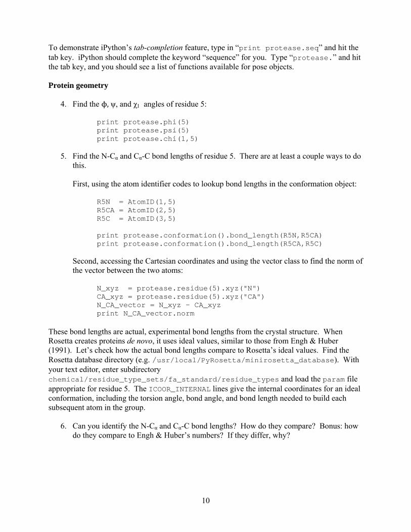
4. Find the , ψ, and χ1 angles of residue 5:

print protease.phi(5) print protease.psi(5) print protease.chi(1,5)

5. Find the N-Cα and Cα-C bond lengths of residue 5. There are at least a couple ways to do this. First, using the atom identifier codes to lookup bond lengths in the conformation object:

R5N = AtomID(1,5) R5CA = AtomID(2,5) R5C = AtomID(3,5) print protease.conformation().bond_length(R5N,R5CA) print protease.conformation().bond_length(R5CA,R5C)

Second, accessing the Cartesian coordinates and using the vector class to find the norm of the vector between the two atoms:

N_xyz = protease.residue(5).xyz("N") CA_xyz = protease.residue(5).xyz("CA") N_CA_vector = N_xyz – CA_xyz print N_CA_vector.norm

These bond lengths are actual, experimental bond lengths from the crystal structure. When Rosetta creates proteins de novo, it uses ideal values, similar to those from Engh & Huber (1991). Let’s check how the actual bond lengths compare to Rosetta’s ideal values. Find the Rosetta database directory (e.g. /usr/local/PyRosetta/minirosetta_database). With your text editor, enter subdirectory chemical/residue_type_sets/fa_standard/residue_types and load the param file appropriate for residue 5. The ICOOR_INTERNAL lines give the internal coordinates for an ideal conformation, including the torsion angle, bond angle, and bond length needed to build each subsequent atom in the group.

6. Can you identify the N-Cα and Cα-C bond lengths? How do they compare? Bonus: how do they compare to Engh & Huber’s numbers? If they differ, why?

11

7. Find the N-Cα-C bond angle:

print protease.conformation().bond_angle(R5N,R5CA,R5C)

Again, compare with the Rosetta database ideal value. What is the hybridization of the Cα atom? What is the standard bond angle for such a hybridization? Be aware that not all bond lengths and angles are accessible through the conformation object. The conformation object only contains a minimal subset of bond lengths and angles used in generating Cartesian coordinates. The vector objects provide a general way to measure angles, distances, and torsions between arbitrary atoms.

8. How could you also find the N-Cα-C bond angle using the vector dot product function,

v3 = v1.dot(v2)?

Manipulating protein geometry

9. We can also alter the geometry of the protein. Perform each of the following manipulations, and give the coordinates of the N atom of residue 6 afterward.

protease.set_phi(5,-60) protease.set_psi(5,-43) protease.set_chi(1,5,180) protease.conformation().set_bond_length(R5N,R5CA,1.5) protease.conformation().set_bond_angle(R5N,R5CA,R5C,110)

Remember that only some bond lengths and angles are available through the conformation object.

Programming

10. We can write programs in Python to accomplish more complicated tasks. Using your text editor, open a new file with extension “.py” (e.g., rama.py). You can write your entire program here, and then run it either from the command line by typing

[linux]> python rama.py

or from inside a Python shell by typing

In [1]: import rama.py

12

Here is a sample program:

from rosetta import * rosetta.init() p = Pose() pose_from_pdb(p,"1abc.pdb") for i in range(1, p.total_residue()+1): print i, " phi = ", p.phi(i), "psi = ", p.psi(i)

Note that we must first initialize Rosetta with the import command, and load the pose. Test that you can write and run a simple program from a file.

Programming exercises Submit your script file and your output.

1. Use the vector objects to write a script to calculate torsion angles between four arbitrary atoms.

2. Ideal helix. Write a program to create a 20-residue ideal helix by setting the and ψ angles to the typical values for an α helix. To start, use make_pose_from_sequence(pose,"AAA","fa_standard"), except use 20 “A”s in the argument to create a 20-residue poly-alanine. Output your structure using helix.dump_pdb("helix.pdb"). View your new file in PyMol to check your work. How can you be sure your structure is a proper α-helix? List three distinct structural characteristics that you can check.

3. Ideal strand. Write a program to create a 20-residue ideal β strand by setting the and ψ angles to values in the middle of the β region of the Ramachandran plot. View your new file in PyMol to check your work. How can you be sure your structure is a proper β-sheet? List three distinct structural characteristics that you can check.

4. Secondary structure propensities. Write a program to calculate the propensity of each residue type to appear in a helix. Loop through all residues in a protein, and count each alanine which is helical, sheet, or loop according to some /ψ based criteria. The propensity can then be calculated as , , and , where Nα, Nβ, NL, and NT are the counts of helical, sheet, loop, and total alanine residues, respectively. Bonus level 1: Find propensities for all 20 amino acid types. This will be easier if you use a data structure like a list or array to store the counts of the 20 types. Do the residues with the highest helical propensity match that given by Brandon & Tooze?

13

Bonus level 2: To get better statistics, collect your data by looping over a set of 10 PDB files. Better yet, use a set of files such as the PDBSelect set of representative chains (http://bioinfo.tg.fh-giessen.de/pdbselect; this may require considerable download and compute time).

5. Idealize a protein. Write a program which sets all bond lengths and angles to their Engh & Huber ideal values. Test your program using a structure from the PDB. What happens to the resulting protein? Why?

References

1. R. A. Engh & R. Huber, “Accurate Bond and Angle Parameters for X-ray Protein Structure Refinement,” Acta. Cryst. A47, 392-400 (1991).

2. J. Parsons et al., “Practical conversion from Torsion Space to Cartesian Space for In Silico Protein Synthesis,” J. Comp. Chem. 26, 1063-1068 (2005).

3. Python help available at http://python.org/doc.

14

Workshop #3: PyRosetta Scoring Scoring Poses A basic function of Rosetta is calculating the energy or score of a biomolecule. Rosetta has a standard energy function for all-atom calculations as well as several scoring functions for low-resolution protein representations. In addition, you can tailor an energy function by including scoring terms of your choice with custom weights. For these exercises, use the protein ras (PDB ID 6Q21) and load it into a pose called ras. Be sure to clean the PDB file and use only one chain.

1. To score a protein, you must first define a scoring function:

scorefxn = create_score_function('standard')

The option for standard tells Rosetta to load the standard all-atom energy terms. To see these terms, you can print the score function:

print scorefxn

What terms are in the score function, and what are their relative weights?

2. Set up your own custom score function which includes just van der Waals, solvation, and hydrogen bonding terms, all with weights of 1.0. Use the following:

scorefxn2=ScoreFunction() scorefxn2.set_weight(fa_atr,1.0) scorefxn2.set_weight(fa_rep,1.0)

Confirm that the weights are set correctly.

3. Evaluate the energy of ras with the standard score function:

scorefxn(ras)

What is the total energy of ras?

15

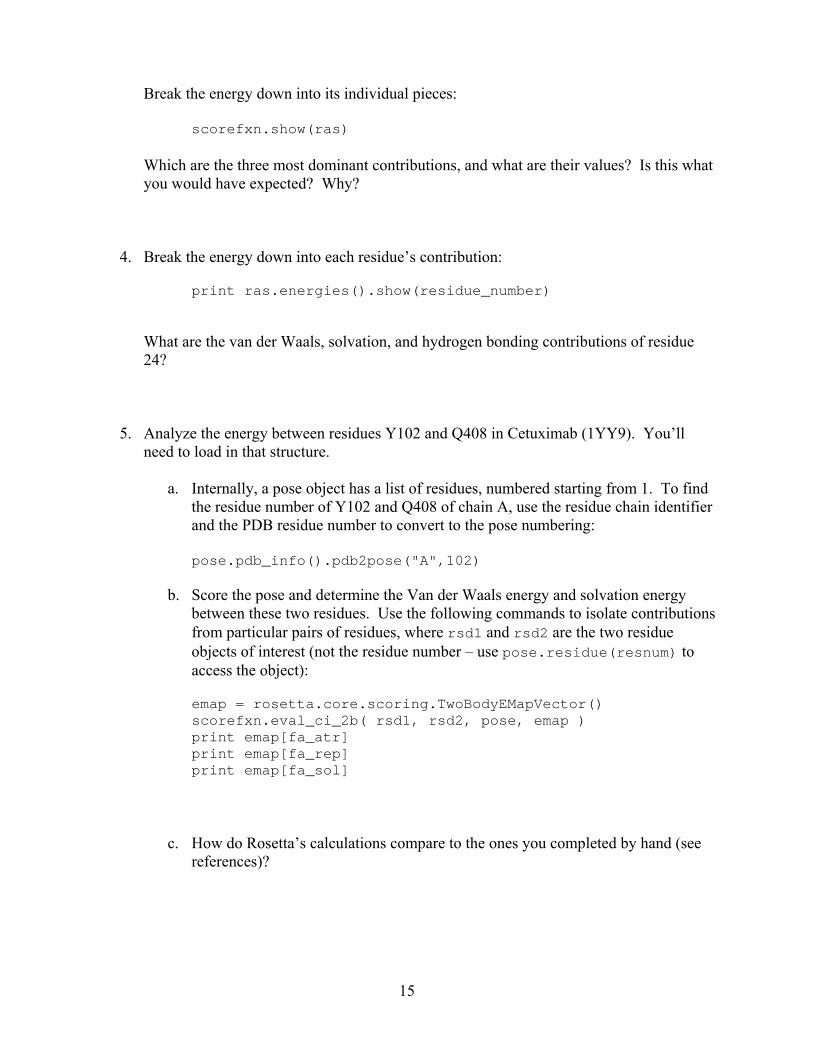
Break the energy down into its individual pieces:

scorefxn.show(ras)

Which are the three most dominant contributions, and what are their values? Is this what you would have expected? Why?

4. Break the energy down into each residue’s contribution:

print ras.energies().show(residue_number)

What are the van der Waals, solvation, and hydrogen bonding contributions of residue 24?

5. Analyze the energy between residues Y102 and Q408 in Cetuximab (1YY9). You’ll

need to load in that structure.

a. Internally, a pose object has a list of residues, numbered starting from 1. To find the residue number of Y102 and Q408 of chain A, use the residue chain identifier and the PDB residue number to convert to the pose numbering: pose.pdb_info().pdb2pose("A",102)

b. Score the pose and determine the Van der Waals energy and solvation energy

between these two residues. Use the following commands to isolate contributions from particular pairs of residues, where rsd1 and rsd2 are the two residue objects of interest (not the residue number – use pose.residue(resnum) to access the object): emap = rosetta.core.scoring.TwoBodyEMapVector() scorefxn.eval_ci_2b( rsd1, rsd2, pose, emap ) print emap[fa_atr] print emap[fa_rep] print emap[fa_sol]

c. How do Rosetta’s calculations compare to the ones you completed by hand (see references)?

16

d. Create a new PDB file containing coordinates for just the two residues Y102 and Q408. Repeat the above calculations. Which energies change? Why?

Programming exercises

1. Interface energy. Write a program that can calculate the binding energy of EGFR to Cetuximab. You will need to make separate PDB files for the antigen, antibody, and complex. In PyMOL, select one of these peptides, then use File→Save Molecule. Use the following formula for binding energy:

Ebinding = Ecomplex – Eantibody – Eantigen

Submit your script along with output values for the total binding energy, Van der Waals, hydrogen bonding and solvation energies. What does your result suggest about these two proteins in vitro? What are some inaccuracies in the way you’ve calculated the binding energy?

2. Statistical energy functions. Write a program to create a histogram of the C-N bond

lengths observed in a set of ten high-resolution x-ray protein structures. (One source of curated structures is the WHATIF sets at http://swift.cmbi.kun.nl/swift/whatif/select).

a. Plot the data as a histogram of probability versus bond length, and also as a statistical free energy versus bond length. Try a bin size of 0.5 Å.

b. Look up the CHARMm potential for this bond stretch, and plot a curve over each of your figures to show the CHARMm model for this motion.

c. Do the statistics match that which would be produced by a harmonic oscillator under the CHARMm potential? Specifically, is the average bond length and the CHARMm spring constant K correct? If not, what should it be? You may need to fit a parabola to your data to find the average bond length and the spring constant K.

References

1. E. Neria, S. Fischer & M. Karplus, “Simulation of activation free energies in molecular systems,” J. Chem. Phys. 105, 1902-1921 (1996).

2. T. Kortemme, A. V. Morozov & D. Baker, “An orientation-dependent hydrogen bonding potential improves prediction of specificity and structure for proteins and protein-protein complexes,” J. Mol. Biol. 326, 1239-1259 (2003).

3. D. Eisenberg & A. D. McLachlan, “Solvation energy in protein folding and binding,” Nature 319, 199-203 (1986).

4. T. Lazaridis & M. Karplus, “Effective energy function for proteins in solution,” Proteins 35, 133-152 (1999).

17

Workshop #4: PyRosetta Folding In this workshop you will write your own Monte Carlo protein folding algorithm from scratch, and we will explore a couple of the tricks used by Simons et al. (1997,1999) to speed up the folding search. Suggested Readings

1. K. T. Simons et al., “Assembly of Protein Structures from Fragments,” J. Mol. Biol. 268, 209-225 (1997).

2. K. T. Simons et al., “Improved recognition of protein structures,” Proteins 34, 82-95 (1999).

3. Chapter 4 (Monte Carlo methods) of M. P. Allen & D. J. Tildesley, Computer Simulation of Liquids, Oxford University Press, 1989.

A simple de novo folding algorithm First, we would like to create a simple folding algorithm. Begin with a new pose, and then create a starting structure using:

pose=Pose() make_pose_from_sequence(pose,"AAAAAAAAAA","fa_standard")

Dump these coordinates and examine briefly in PyMol. You should see ideal bond lengths and angles, although the set of /ψ angles will not be useful. Write a program which implements a Monte Carlo algorithm to optimize the protein conformation. In the main program, create a loop with 100 iterations. Each iteration should call a subroutine to make a random trial move, and then score the protein, and then accept or reject the new conformation based on the Metropolis criteria. Use kT = 1. For the random trial move, write a subroutine to choose one residue at random and then randomly perturb either the φ or ψ angles by a random number chosen from a Gaussian distribution with a standard deviation of 25°. Use the Python built-in random.gauss() from the random library. For the energy function, use the standard full-atom scoring approach with only the van der Waals and hydrogen bonding terms. With this scoring function, what kind of structures do you expect to be most stable? At each iteration of the search, output the current pose energy and the lowest energy ever observed. The final output of this program should be the lowest energy conformation that is achieved at any point during the simulation. Be sure to use low_pose.assign(pose) rather than low_pose = pose, since the latter will only copy a pointer to the original pose.

18

1. Output the last pose and the lowest-scoring pose observed, and view them in PyMol. Plot the energy and lowest-energy observed vs. cycle number. What are the energies of the initial, last, and lowest-scoring pose? Is your program working? Has it converged to a good solution?

2. Using the program you wrote for workshop 2, force the A10 sequence into an α-helix. Does this structure have a lower score than that produced by your algorithm? What does this mean about your sampling or discrimination?

3. Since your program is a stochastic search algorithm, it may not produce an ideal structure consistently, so try running the simulation multiple times or with a different number of cycles (if necessary). Using a kT of 1, your program may need to make up to 500,000 iterations.

Low-resolution (centroid) scoring Following the treatment of Simons et al. (1999), Rosetta can score a protein conformation using a low-resolution representation. This will make the energy calculation faster.

4. Load a protein with which you are familiar (e.g. ras or Cetuximab). Calculate the full-atom energy and note the coordinates of residue 5 using print pose.residue(5).

5. Convert the pose to the centroid form by using the SwitchResidueTypeSetMover:

switch = SwitchResidueTypeSetMover('centroid') switch.apply(pose) print pose.residue(5)

How many atoms are now in residue 5? How is this different than before?

6. Score the new, centroid-based pose using the standard score function score3. What is the new total score? What scoring terms are included in score3? Do these match Simons?

19

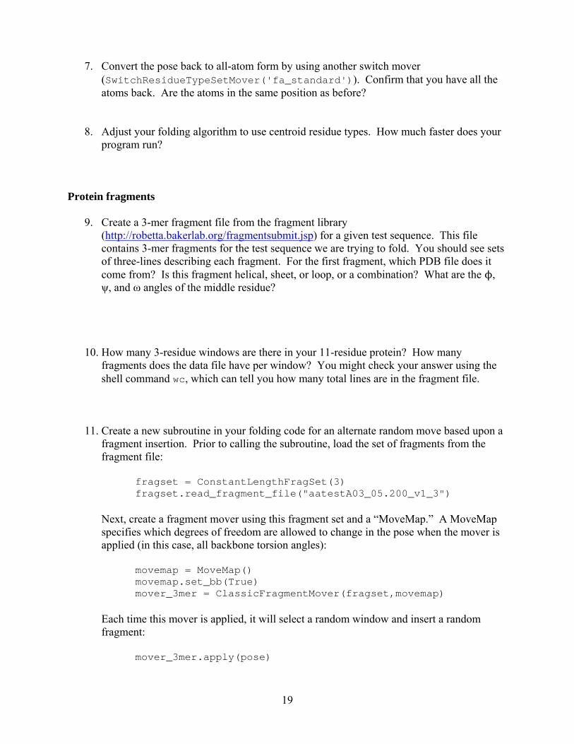
7. Convert the pose back to all-atom form by using another switch mover (SwitchResidueTypeSetMover('fa_standard')). Confirm that you have all the atoms back. Are the atoms in the same position as before?

8. Adjust your folding algorithm to use centroid residue types. How much faster does your program run?

Protein fragments

9. Create a 3-mer fragment file from the fragment library (http://robetta.bakerlab.org/fragmentsubmit.jsp) for a given test sequence. This file contains 3-mer fragments for the test sequence we are trying to fold. You should see sets of three-lines describing each fragment. For the first fragment, which PDB file does it come from? Is this fragment helical, sheet, or loop, or a combination? What are the , ψ, and ω angles of the middle residue?

10. How many 3-residue windows are there in your 11-residue protein? How many fragments does the data file have per window? You might check your answer using the shell command wc, which can tell you how many total lines are in the fragment file.

11. Create a new subroutine in your folding code for an alternate random move based upon a fragment insertion. Prior to calling the subroutine, load the set of fragments from the fragment file:

fragset = ConstantLengthFragSet(3) fragset.read_fragment_file("aatestA03_05.200_v1_3")

Next, create a fragment mover using this fragment set and a “MoveMap.” A MoveMap specifies which degrees of freedom are allowed to change in the pose when the mover is applied (in this case, all backbone torsion angles):

movemap = MoveMap() movemap.set_bb(True) mover_3mer = ClassicFragmentMover(fragset,movemap)

Each time this mover is applied, it will select a random window and insert a random fragment:

mover_3mer.apply(pose)

20

When you change your random move to a fragment insertion, how much faster is your folding code? Does it converge to a protein-like conformation more quickly?


1. Fold a 10-mer poly-alanine using 100 independent trajectories (use any variant of the folding algorithm that you like). Create a Ramachandran plot using the lowest-scoring conformations from all 100 independent trajectories. Repeat this for an 10-mer poly-glycine. How do the plots differ? Compare with the plots in Richardson’s article.

2. Test your folding program’s ability to predict a real fold from scratch. Choose a small

protein to keep the computation time down, such as Hox-B1 homeobox protein (1b72) or RecA (2reb). How many iterations and how many independent trajectories do you need to run to find a good structure?

3. Modify your folding program to include a simulated annealing temperature schedule, decaying exponentially from kT = 100 to kT = 0.1 over the course of the search. Again, fold a test protein. Does this approach work better?

4. Modify your folding program to remove the Metropolis criterion and instead accept trial moves only when the energy decreases. Plot energy vs. iteration, and examine the final output structures from multiple runs. How is the convergence and performance affected? Why?

Thought questions

1. [advanced] How might you design an intermediate-resolution representation of side chains that has more detail than the centroid approach yet is faster than the full atom approach? Which types of residues would most benefit from this type of representation?

2. [introductory] What are the limitations of these types of folding algorithms?

21

Workshop #5: PyRosetta Refinement Suggested Reading

1. P. Bradley, K. M. S. Misura & D. Baker, “Toward high-resolution de novo structure prediction for small proteins,” Science 309, 1868-1871 (2005), including Supplementary Material.

2. Z. Li & H. A. Scheraga, “Monte Carlo-minimization approach to the multiple-minima problem in protein folding,” Proc. Natl. Acad. Sci. USA 84, 6611-6615 (1987).

One of the most basic operations in protein structure and design algorithms is manipulation of the protein conformation. In Rosetta, these manipulations are organized into Movers. A Mover object simply changes the conformation of a given pose. It can be simple like a single or ψ angle change, or complex like an entire refinement protocol. In the last workshop, you encountered the ClassicFragmentMover, which inserts a short sequence of backbone torsion angles, and the SwitchResidueTypeSetMover, which doesn’t actually change the conformation of the pose but instead swaps out the residue types used. In this workshop, we will introduce a variety of other movers, particularly those used in high-resolution refinement (e.g., in Bradley’s 2005 paper). Before you start, load a test protein and make a copy of the pose so we can compare:

start = Pose() pose_from_pdb(start, "test_in.pdb") test = Pose() test.assign(start)

Small and shear moves The simplest move types are small moves, which perturb or ψ of a random residue by a random small angle, and shear moves, which perturb of a random residue by a small angle and ψ of the same residue by the same small angle of opposite sign. For convenience, the small and shear movers can do multiple rounds of perturbation. They also check that the new /ψ combinations are within an allowable region of the Ramachandran plot by using a Metropolis acceptance criterion based on the rama score change. (The rama score is a statistical score from Simons et al. 1999, parametrized by bins of /ψ space.) Finally, like most movers, these require a MoveMap to specify which degrees of freedom are fixed and which are free to change. Thus, we can create our movers like this:

kT = 1.0 n_moves = 1 movemap = MoveMap() movemap.set_bb(True) smallmover = SmallMover(movemap,kT,n_moves)

22

shearmover = ShearMover(movemap,kT,n_moves) We can also adjust the maximum magnitude of the perturbations as follows:

smallmover.angle_max('H',25) smallmover.angle_max('E',25) smallmover.angle_max('L',45)

Here, H, E, and L refer to helical, sheet, and loop residues, and the magnitude is in degrees. Set all the maximum angles to 25° to make the changes easy to visualize.

1. Test your mover by applying it to your pose:

smallmover.apply(test)

Confirm that the change has occurred by one of two methods: (1) use your old program for printing the /ψ angles of the start and test poses to find the change or (2) use dump_pdb to output the poses to files, and compare the structures in PyMol. Alternately, you could write a quick program to compare the poses. Which torsion angles changed? By how much?

2. Comparing small and shear movers. Reset the test pose by re-assigning it a

conformation from the start position, and create a second test pose in the same manner. Reset the existing MoveMap object to only allows backbone angles of residue 50 to move (Hint: set all residues to False, then set just residues 50 and 51 to True using movemap.set_bb(50,True) and movemap.set_bb(51,True). Note that the SmallMover is connected to your MoveMap and it will automatically know you have made these changes and use the modified MoveMap in future moves. Make one small move on one of your test poses, and one shear move on the other test pose. Output all the poses to files and view them in PyMol (show only backbone atoms and view as lines or sticks). Identify the torsion angle changes that occurred. What was the magnitude of the change in sheared pose? How does the displacement of residue 60 compare between the small- and shear-perturbed poses?

Minimization moves The MinMover carries out a gradient-based minimization to find the nearest local minimum in the energy function, such as that used in one step of the Monte-Carlo-plus-Minimization algorithm of Li & Scheraga.

minmover = MinMover()

23

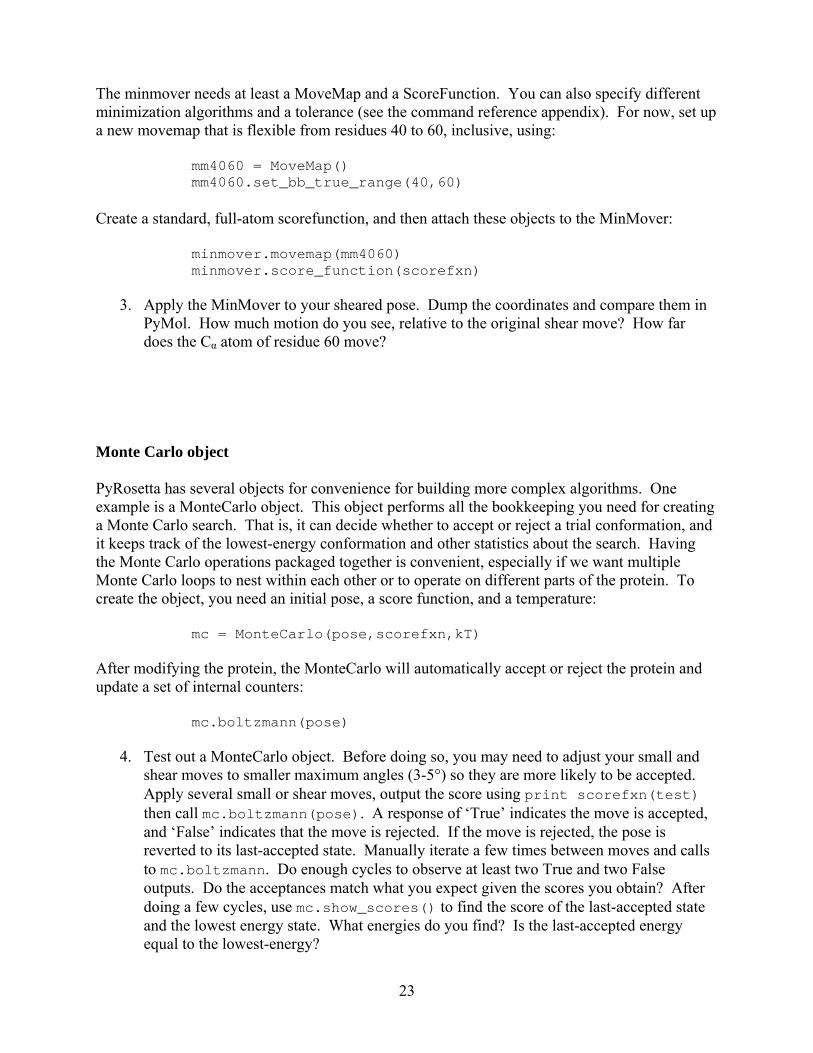
The minmover needs at least a MoveMap and a ScoreFunction. You can also specify different minimization algorithms and a tolerance (see the command reference appendix). For now, set up a new movemap that is flexible from residues 40 to 60, inclusive, using:

mm4060 = MoveMap() mm4060.set_bb_true_range(40,60)

Create a standard, full-atom scorefunction, and then attach these objects to the MinMover:

minmover.movemap(mm4060) minmover.score_function(scorefxn)

3. Apply the MinMover to your sheared pose. Dump the coordinates and compare them in PyMol. How much motion do you see, relative to the original shear move? How far does the Cα atom of residue 60 move?

Monte Carlo object PyRosetta has several objects for convenience for building more complex algorithms. One example is a MonteCarlo object. This object performs all the bookkeeping you need for creating a Monte Carlo search. That is, it can decide whether to accept or reject a trial conformation, and it keeps track of the lowest-energy conformation and other statistics about the search. Having the Monte Carlo operations packaged together is convenient, especially if we want multiple Monte Carlo loops to nest within each other or to operate on different parts of the protein. To create the object, you need an initial pose, a score function, and a temperature:

mc = MonteCarlo(pose,scorefxn,kT)

After modifying the protein, the MonteCarlo will automatically accept or reject the protein and update a set of internal counters:

mc.boltzmann(pose)

4. Test out a MonteCarlo object. Before doing so, you may need to adjust your small and shear moves to smaller maximum angles (3-5°) so they are more likely to be accepted. Apply several small or shear moves, output the score using print scorefxn(test) then call mc.boltzmann(pose). A response of ‘True’ indicates the move is accepted, and ‘False’ indicates that the move is rejected. If the move is rejected, the pose is reverted to its last-accepted state. Manually iterate a few times between moves and calls to mc.boltzmann. Do enough cycles to observe at least two True and two False outputs. Do the acceptances match what you expect given the scores you obtain? After doing a few cycles, use mc.show_scores() to find the score of the last-accepted state and the lowest energy state. What energies do you find? Is the last-accepted energy equal to the lowest-energy?

24

5. See what information is stored in the Monte Carlo object using:

mc.show_scores() mc.show_counters() mc.show_state()

What information do you get from each of these?

Trial Mover A TrialMover combines a mover with a Monte Carlo object. Each time a TrialMover called, it performs a trial move and tests that move’s acceptance with the MonteCarlo object. You can create a TrialMover from any other type of mover. You might imagine as we start nesting these together, we can build some complex algorithms!

trialmover = TrialMover(smallmover, mc) trialmover.apply(pose)

6. Apply the TrialMover above ten times. Using trialmover.num_accepts() and trailmover.acceptance_rate(), what do you find?

7. The TrialMover also communicates information to the MonteCarlo object about the type of moves being tried. Create a second TrialMover using a ShearMover and the same MonteCarlo object, and apply this second TrialMover ten times. Look at the MonteCarlo object state (mc.show_state()). What are the acceptance rates of each mover? Which mover is accepted most often, and which has the largest energy drop per trial? What are the average energy drops?

Sequence and Repeat Movers A SequenceMover applies several movers in succession and is useful for building up complex routines.

seqmover = SequenceMover() seqmover.add_mover(smallmover) seqmover.add_mover(shearmover) seqmover.add_mover(minmover)

25

This mover will apply first the small, then the shear mover, and finally the minmover.

8. Create a TrialMover using the sequence mover above, and apply it five times to the pose. How is the sequence mover shown by mc.show_state()?

A RepeatMover will apply its input mover multiple times each time it is applied:

repeatmover = RepeatMover(trialmover,10)

9. Use these tools to build up your own ab-initio protocol. Create TrialMovers for 9-mer and 3-mer fragment insertion. Create RepeatMovers for each, and then create TrialMovers for each using the same MonteCarlo object. Create a SequenceMover to do the 9-mer trials and then the 3-mer trials, and iterate the sequence 10 times. Write out a flowchart of your algorithm here:

10. Hierarchical search. Write a TrialMover which tries to insert a 9-mer fragment, and then refines the protein with 100 alternating small and shear trials before the next 9-mer fragment trial. The interesting part is this: you will use one MonteCarlo object for the small and shear trials, inside the whole 9-mer combination mover. But use a separate MonteCarlo object for the 9-mer trials. In this way, if a 9-mer fragment insertion is evaluated after the optimization by small and shear moves, and if it is rejected, the pose goes all the way back to before the 9-mer fragment insertion.

Refinement Protocol The standard Rosetta refinement protocol, similar to that presented in Bradley, Misura & Baker 2005 is available as a mover. Note that the protocol can require ~40 minutes for a 100-residue protein.

relax = ClassicRelax() relax.apply(pose)

26


1. Use the mover constructs to create a complex folding algorithm. Create a simple program to do the following:

a. Five small moves b. Minimize c. Five shear moves d. Minimize e. Monte Carlo Boltzmann step f. Repeat a-e 100 times g. Repeat a-f five times, each time decreasing the magnitude of the small and shear

moves from 25° to 5° in 5° increments.

Sketch a flowchart, and submit both the flowchart and your code.

2. Ab initio folding algorithm. Using the Monte Carlo energy optimization algorithm from Workshop 4, write a complete program that will fold a protein. A suggested algorithm involves preliminary low-resolution modifications by fragment insertion (first 9-mers, then 3-mers), followed by high-resolution refinement using small, shear, and minimization movers, as well as side-chain packing. Test your code by attempting to fold a zinc finger. How do your results compare with the crystal structure? If your lowest-energy conformation is different than the native structure, explain why this is so in terms of the limitations of the computational approach. Bonus: Dump the pose coordinates as you go and use PyMol to create an animation.

3. AraC N-terminal arm. The AraC transcription factor is believed to be activated by the conformational change which occurs in the N-terminus when arabinose binds. Let’s test whether PyRosetta can capture this change. Specifically, we will start with the arabinose-bound form, and see if PyRosetta can refold it to the apo form. Download the arabinose-bound form of the AraC transcription factor. Edit the PDB file so it contains only the arabinose-binding domain, and also remove any non-protein atoms (especially the arabinose). Set up a move map to include only 15 N-terminal residues. Perform an ab-initio search to find the lowest conformation state. How does it compare to the apo crystal form?

Thought questions

1. With kT = 1, what is the change in propensity of the rama score that has a 50% chance of being accepted as a small move?

2. How would you test whether an algorithm is effective? That is, what kind of measures can you use? What can you vary within an algorithm to make it more effective?

27

Workshop #6: Packing & Design Suggested readings

1. J. Desmet et al., “The dead-end elimination theorem and its use in protein side-chain positioning,” Nature 356, 539-543 (1992).

2. B. Kuhlman & D. Baker, “Native protein structures are close to optimal for their structures,” PNAS 97, 10383, 2000.

Rosetta uses a Monte Carlo optimization routine to pack side chains using a library of conformations, or rotamers. This operation can be used for side-chain packing for operations like refinement or for designing optimal sequences. This workshop will examine both capabilities. Side-chain conformations, the rotamer library, and Dunbrack energies Begin by loading cetuximab from PDB 1YY8.

1. What are the , ψ, and χ angles of residue K49?

2. Open the file lys.*.bbdep.regular.lib from the minirosetta_database/dun?? directory. Find the /ψ bin for the K49 position and find the nearest rotamer. What are the χ angles and standard deviations of this rotamer? What is its probability?

3. Score your pose with the standard full-atom score function. What is the energy of K49? Note the Dunbrack energy component (fa_dun), which represents the side-chain conformational probability. Does it match that which you found in the table (you will need to convert probability to energy; use kT = 1)? If not, why not?

4. Use pose.set_chi(i,j,chi) to set the side chain of residue 49 to the all-trans conformation (here, i is the χ index, j is the residue number, and chi is the new torsion angle in degrees). Re-score the pose and note the Dunbrack energy. Does it match the probabiltity in the table? Is this conformation valid for Cetuximab (i.e., is the total score of this residue acceptable)?

28

Monte Carlo side-chain packing Side-chain packing can be done in a Monte Carlo search routine which iteratively swaps rotamers of a random residue and tests each move using the Metropolis criterion. Rosetta has such a routine pre-packaged as a mover which carries out a simulated annealing search each time it is applied. The specific scope of the packing is specified in a PackerTask object, which we can specify via commands or from an input file. Create a PackerTask as follows. This will set the task to allow packing only of residue 49:

task_pack = standard_packer_task(pose) task_pack.restrict_to_repacking() task_pack.fix_everything() task_pack.set_pack_residue(49,True)

Confirm your settings using

print task_pack We now can create a PackRotamersMover:

packmover = PackRotamersMover(scorefxn,task_pack)

5. Apply the packmover to your pose with packmover.apply(pose). Now what are the χ angles of K49? Which rotamer is this? What is the Dunbrack energy?

6. What is the new total energy of K49? Why did Rosetta pick this rotamer? Answer this in terms of the components of the score function and in terms of the residues with which K49 interacts.

Packing for refinement Side-chain packing can be used when converting a pose from centroid to full-atom mode, and it is used extensively in full-atom refinement calculations. Let’s examine how packing improves scores. Use your code from last week to create a centroid-representation model for a zinc-finger sequence (or use one of your structures from the last workshop). Save that centroid “decoy” so that we can compare several basic refinement steps.

29

7. Load the centroid decoy and convert it to full-atom representation using the SwitchResidueTypeSetMover. Save this starting configuration for future use. Score the pose. Why is the score so high?

8. Create a default PackRotamersMover with a PackerTask that allows all residues to vary χ angles. Create a test pose from your start pose and pack the side chains. What is the new pose score?

9. Reset the test pose to the start configuration. Create a MinMover using the ‘dfpmin’ minimization scheme. Create a MoveMap that allows χ angles but not /ψ/ω angles to vary. Apply the MinMover and rescore the pose. How does this energy compare?

10. Again reset the test pose. This time convert the pose to full-atom representation, apply the packer, and then minimize on the χ angles. Now what is the final score?

For fun, you might examine the individual residue energies to find the residues most responsible for the score changes. Typically, a small number of residues may make clashes which can be resolved using the χ angle minimization, which allows off-rotamer side-chain conformations. Design Design calculations can be accomplished simply by packing side chains with a rotamer set that includes all amino acid types. That is, when the Monte Carlo routine swaps rotamers, it could replace the exiting side chain with another conformation of the same residue, or some conformation of a different residue type. Trial mutations are accepted with the Metropolis criterion, and the standard full-atom energy function is supplemented by a reference energy term which represents the relative energies of each residue type in an unfolded peptide. Design operations are easiest to specify through a data file called a “resfile.” You can create a resfile for a given pdb file or pose using:

generate_resfile_from_pdb("1YY8.pdb","1YY8.resfile") generate_resfile_from_pose(pose,"1YY8.resfile")

Inside the resfile you will see a list of all residues and NATRO next to it, indicating that it is set to use the native rotamer. NATRO can be changed to the following:

30

NATRO use native amino acid and native rotamer (does not repack) NATAA use native amino acid, but allow repacking to other rotamers PIKAA ILV use only the following amino acids and allow repacking between them ALLAA use all amino acids and all repacking Edit the resfile to allow force residue 49 to be glutamic acid (“49 A PIKAA E”) and save the file as 1YY8-K49E.resfile. Create a new task for design from the resfile:

task_design = TaskFactory.standard_packer_task(pose) task_design.read_resfile("1YY8-K49E.resfile")

11. Score the original conformation from the pdb for reference. Create a new

PackResiduesMover with the design task and use it to mutate residue 49 to glutamic acid. What is the predicted ΔG of the mutation? Is this a stabilizing mutation?

12. Note the residue reference energy term (“ref”) in the scoring function. What is this value before and after you mutated the residue? What does this energy represent?

13. Create a new PackerTask and PackRotamersMover using a new resfile which allows residue 49 to be designed freely (“49 A ALLAA”), and apply the mover. What residue does Rosetta choose? Why?

14. Create your own resfile which will restrict residue 49 to only negatively charged residues

using the resfile line “49 A PIKAA DE” and re-apply the design mover. Now what residue is chosen? What is the new residue energy, and why (physically) is it less favorable than the last design?

15. Let’s try to make this design more favorable. Select several surrounding residues for design, and set them also to enable mutations to any residue. Call the design mover again. Now what do you find?


1. Refinement and discrimination. Download the “single misfold” decoy set from the Decoys ‘R Us repository at dd.compbio.washington.edu/ddownload.cgi?misfold.

31

(Documentation for this project is at dd.compbio.washington.edu.) This repository has a single “correct” and “incorrect” predicted structure for several proteins. For this exercise, analyze pdbs 2ci2 and 2cro; each has two “incorrect” structures offered. (Technical note: These decoys have an empty Occupancy field in the PDB ATOM records; a value of 1 needs to be added before Rosetta will load these structures.) Write a program which will calculate and output the score for each decoy (i) as is from the PDB file (ii) after packing only (iii) after minimization only (iv) after packing and minimizing. For each of the four cases, compare the scores of the “correct” structure with those of the “incorrect” structure. Which schemes successfully discriminate the correct structures?

2. Write a refinement protocol which will iterate between side-chain packing, small and

shear moves, and minimization. Where is the best place to position the Monte Carlo acceptance test? Test your protocol by making 10 independently-refined structures for the correct and incorrect decoys of 2cro from the Decoys ‘R Us single misfold set. Is this protocol able to discriminate the correct decoy? Submit your code.

3. HIV-1 protease is a major drug target for antiretroviral therapies. Protease inhibitors are

designed from substrate peptide mimics. We will attempt to take a natural substrate peptide of HIV-1 protease and design it for improved binding—potentially to serve as a good template for drug design. Use PDB file 1kjg for the following analysis.

a. Turn on side-chain packing for the protease active site (residues 8, 23, 25, 29, 30, 32, 45, 47, 50, 53, 82 and 84 of both chain A and B) and for the peptide (residues 2-9 on chain P; all of these numbers follow the PDB numbering).

b. Repack the above side chains and then energy minimize those same side chains with the backbone fixed. Generate 10 decoys and record the energies for each decoy. This will represent the reference state: the wild-type peptide bound to the protease.

c. For residue 2 of the peptide (chain p) allow repacking to any of the 20 amino acids, while leaving the packing and side-chain minimization the same as in step 3. Generate 10 decoys and record the energies. These will represent single mutants at that residue position.

d. Repeat step c for each of the other 8 residues in the substrate peptide. e. Take the lowest energy for each mutation position and compare it the lowest

energy for the wild type. Do single mutants at any of these positions improve the energy over the wild type? Which ones? By how much? Which energy components are mostly responsible?

f. What peptide residue positions are easiest to improve on? Which positions are the hardest?

g. Are there any other trends? Hydrophobic vs. polar, bulky residues vs. small residues, etc.

h. Altman et al. (Proteins 2008) found, using their own computational design algorithm, that the most favorable sequences were a triple mutant E3D/T4I/V6L, a single mutant T4V, and a single mutant D3Q. How do their results compare with yours?

32

i. Natural substrates are often sub-optimal binders. Why would this be advantageous?

4. Effect of backbone conformation on design. HIV-1 protease is promiscuous, meaning it

can cleave a wide range of peptides beyond the ten natural substrates of the virus. Let’s examine the preferences of the enzyme through Rosetta design calculations.

a. Download the complex of HIV-1 protease in complex with CA-P2 peptide (1f7a). Select the eight peptide residues for unrestricted design and let Rosetta redesign the substrate sequence. What is the new sequence and how does it compare to the original? What percent of the original sequence was optimal for its structure?

b. Download the complex of HIV-1 protease in complex with RT-RH peptide (1kjg). Note that the enzyme is the same here, but it is crystallized with a different substrate. Again, design the eight substrate residues with Rosetta. What percent of this substrate sequence is optimal for this crystal structure?

c. How do the designed sequences of (a) and (b) compare? Why should they be the same? Why would they not be the same? What are the implications for the field of computational protein design?

5. Write a program which iterates between design of all residues of a protein and

refinement via small, shear, and minimization moves. Thought questions

1. Amino acid reference energy a. What is the thermodynamic meaning of the ref energy term, and what does it

correspond to physically? b. During evolution, the genome sequence may mutate to cause protein sequence

changes. Alternately, one could consider the difference in evolutionary propensities for each residue type. How could you derive reference energies from sequence data, and what would that mean?

c. How do Kuhlman & Baker fit the reference energies in their 2000 PNAS paper? References

1. S. C. Lovell et al., “The penultimate rotamer library,” Proteins 40, 389-408 (2000). 2. R. L. Dunbrack & F. E. Cohen, “Bayesian statistical analysis of protein side-chain

rotamer preferences,” Protein Sci. 6, 1661-1681 (1997).

33

Workshop #7: Docking Protein-protein docking is the prediction of a complex structure starting from its monomer components. The search space can be extremely large, so large amounts of computational resources are typically required. In this workshop, we will explore several of the techniques briefly; keep in mind that for real applications, many more decoys will need to be tested.

Suggested Readings

1. J. J. Gray et al., “Protein-protein docking with simultaneous optimization of rigid-body displacement and side-chain conformations,” J. Mol. Biol. 331, 281-299 (2003).

2. S. Chaudhury & J. J. Gray, “Conformer selection and induced fit in flexible backbone protein-protein docking using computational and NMR ensembles,” J. Mol. Biol. 381, 1068-1087 (2008).

Fast-Fourier transform based docking via ZDOCK There are several servers available based on fast Fourier transforms. These servers are able to quickly carryout a global, grid-based matching search.

1. Go to the ZDOCK server (http://zdock.bu.edu) and upload α-chymotrypsin (5CHA chain A) and eglin C (1CSE chain I) for docking. If completing this workshop for a class, do this in groups in order to not overload the server. When the jobs have finished (typically under an hour), download the top five models. Are these models similar or diverse? How so?

2. Are any of the models similar to the crystal structure of the bound complex (1ACB)? Other servers include SmoothDock (http://structure.pitt.edu/servers/smoothdock), ClusPro (http://nrc.bu.edu/cluster), Haddock (http://haddock.chem.uu.nl), and GRAMM-X (http://vakser.bioinformatics.ku.edu/resources/gramm/grammx). Any of these provide global docking services to create models which might be useful for refinement by RosettaDock. Docking moves in Rosetta For the following exercises, you may use either the bound complex of α-chymotrypsin or the unbound components. To use the unbound components, you will first need to make a pdb file which has coordinates of both chains (e.g., use the Linux command cat or use a text editor). The fundamental docking move is a rigid-body transformation consisting of a translation and rotation. Any rigid body move also needs to know which part moves and which part is fixed. In

34

Rosetta, this division is known as a “jump” and the set of protein segments and jumps are stored in an object called a “fold tree.” These objects are set up for you by the DockingProtocol object:

DockingProtocol().setup_foldtree(pose) DockingProtocol().setup_foldtree(pose, “E_I”) print pose.fold_tree()

3. In the fold tree printout, each three number sequence is the beginning and ending residue number, then a code. The codes are “-1” for stretches of protein and “1” for a jump. How many jumps are there in your pose?

You can see the type of information in the jump by printing it from the pose:

jump_num = 1 print pose.jump(jump_num)

4. Write out the rotation matrix and the translation vector defined by the jump.

The two basic manipulations are translations and rotations. For translation, the change in x, y, and z coordinates are needed as well as the jump number. A rotation requires a center and an axis about which to rotate. The rigid-body displacement can be altered directly with the RigidBodyTransMover for translations or the RigidBodySpinMover for rotations. For structure prediction calculations, we have a Mover which is preconfigured to make random movements of set magnitudes (in this case, 8° rotation and 3 Å translation):

pert_mover = RigidBodyPerturbMover(jump_num, 3,8 )

5. Apply the RigidBodyPerturbMover to a pose and output the structure to a file. Load the structure into PyMol to confirm the motions are what you expect. What are the new rotation matrix and translation vector in the jump? How many Ångstroms did the downstream protein move?

Global perturbations are useful for making completely randomized starting structures. The following mover will rotate a protein about its geometric center. The final orientation is equally distributed over the ‘globe’.

randomize1 = RigidBodyRandomizeMover(pose, jump_num, partner_upstream)

randomize2 = RigidBodyRandomizeMover(pose, jump_num, partner_downstream)

35

6. Apply both movers to the starting structure, and view the structure in PyMol (you might view it along with the original pose). Does the new conformation look like a candidate docked structure yet?

Since proteins are not spherical, sometimes the random orientation creates severe clashes between the docking partners, and other times it places the partners so they are not longer touching. The DockingSlideIntoContactMover will translate the downstream protein along the line of protein centers until the proteins are in contact.

slide = DockingSlideIntoContact(jump_num) slide.apply(pose)

The MinMover, which we have previously used to change torsion angles to find the nearest minimum in the score function, can also operate on the jump translation and rotation. It suffices to set the jump variable as moveable in the MoveMap:

movemap = MoveMap() movemap.set_jump(jump_num, True) minmover = MinMover() minmover.movemap(movemap) minmover.score_function(scorefxn) # use any scorefxn minmover.apply(pose)

7. Apply the MinMover. How much does the score change? What are the new rotation

matrix and translation vector in the jump? How many Ångstroms did the downstream protein move?

Low-resolution docking via RosettaDock RosettaDock can also perform global docking runs, but it can require significant time. Typically, 105 to 106 decoys are needed in a global run. For this workshop, we will create a much smaller number and learn the tools needed to handle large runs. Docking is available as a Mover which completely encompasses the protocol. To use the mover, you will need a starting pose with both chains and a jump defined. The structure must be in low-resolution (centroid) mode (use the SwitchResidueTypeSetMover), and you will need a low-resolution score function:

scorefxn_low = create_score_function('interchain_cen') Create low-resolution structures as follows:

dock_lowres = DockingLowRes(scorefxn_low,jump_num) dock_lowres.apply(pose)

36

8. You can compare structures by calculating the root-mean-squared deviation of all the Cα

atoms, using CA_rmsd(pose1,pose2). In docking, a more useful measure is the ligand RMSD, which is the deviation of the backbone Cα atoms of the ligand after superposition of the receptor protein backbones. You can calculate ligand RMSD with DockingProtocol().calc_Lrmsd(pose1, pose2). Using both measures, how far did your pose move from the low-resolution search?

9. Examine the decoy created in PyMol. Does it look like a reasonable structure for a protein-protein complex? Explain.

Job distributor For exhaustive searches with Rosetta (docking, refinement, or folding), it is necessary to create a large number of candidate structures, termed decoys. This is often accomplished by spreading out the work over a large number of computers. Additionally, each decoy created needs to be individually labeled. The object which is responsible for managing the output is called a Job Distributor. Here, we will use a simple job distributor to create multiple structures. The following constructor sets the job distributor to create 10 decoys, with filenames like output1.pdb, output2.pdb, etc. The pdb files will also include scores according to the ScoreFunction provided.

jd = PyJobDistributor("output",10,scorefxn_low)

It is also useful to compare each decoy to the native structure (if it is known, otherwise any reference structure can be used). The job distributor will do the rmsd calculation and final scoring upon output. Set the native pose:

Pose native_pose("1aaa.pdb") jd.native_pose = native_pose

Now, run the low-resolution docking protocol to create a structure, and output a decoy:

dock_lowres.apply(pose) jd.output_decoy(pose)

Do this twice and confirm that you have two output files. We can finish the set by using the JobDistributor to set up a loop:

while (jd.job_complete == False): pose.assign(starting_pose) dock_lowres.apply(pose) jd.output_decoy(pose)

37

Note the jd.job_complete Boolean that indicates whether all 10 decoys have been created.

10. Run the loop to create 10 structures. The job distributor also creates a score file, output.sc, which summarizes the energies and rmsds of all structures created. Examine that file. What is the lowest score? What is the lowest energy?

11. Reset the JobDistributor to create 100 decoys (or more or less, as the speed of your processor allows) by reconstructing it. Rerun the loop above to make 100 decoys. Use your score file to plot score versus rmsd. Two easy ways to do this are to import the score file into Excel, or to use the linux command gnuplot. Do you see a funnel?

High-resolution docking The high-resolution stage of RosettaDock is also available as a Mover. This mover encompases random rigid-body moves, side-chain packing, and gradient-based minimization in the rigid-body coordinates. High-resolution docking needs an all-atom score function. The optimized docking weights are available as a patch to the standard all-atom energy function. scorefxn_high = create_score_function_ws_patch('standard','docking') dock_hires = DockingHighRes(scorefxn_high,jump_num)

A high-resolution decoy needs side chains. One way to place the side chains is to call the PackMover, which will generate a conformation from rotamers. A second way is to copy the side chains from the original monomer structures. This is often helpful for docking calculations since the monomer crystal structures have good side chain positions.

recover_sidechains = ReturnSidechainMover(starting_pose) recover_sidechains.apply(pose)

12. Load one of your low-resolution decoys, add the side chains from the starting pose, and

refine the decoy using high-resolution docking. How far did the structure move during refinement? How much did the score improve?

Starting from your lowest-scoring low-resolution decoy, create three high-resolution decoys (you might use the JobDistributor). Do the same starting from the native structure.

13. How do the refined-native scores compare to the refined-decoy scores?

38

14. What is the rmsd of the refined native? Why is it not zero?

15. How much variation do you see in the refined native scores? In the refined decoy scores? Is the difference between the refined natives and the refined decoys significant?

Docking Funnel

16. Using a job distributor, create 10 decoys starting with a randomize2 perturbation, 10 decoys starting from different local random perturbations (8°, 3 Å), 10 decoys starting from low-resolution decoys, and 10 starting from the native structure. Plot all of these points on a funnel plot. How is the sampling from each method? Does the scoring function discriminate good complexes?

Conformer Selection for Ensemble Docking Ensemble docking can use multiple backbones for one or both docking partners. One application is the use of NMR structures for docking. NMR pdb files include multiple models (typically 30-50), all of which are reasonable solutions to the spectroscopy constraints.

17. Load the NMR file of 1EGL. How many models are in this structure? During docking, conformers can be changed using the ConformerSwitchMover. Construct the mover with the ensemble of backbones:

conformerswitch = ConformerSwitchMover(239,301,jump_num, scorefxn_low,"1EGL.pdb")

18. Apply the conformer selection mover and confirm that the backbone changed by

inspecting the and ψ angles. Write down a pair of old and new ( ,ψ) values and the residue number.

19. Write a conformer selection docking procedure which alternates between RigidBodyPerturbMoves and ConformerSwitchMoves. Loop through both moves 50 times. Run this code starting from the native structure. Is the final backbone selected close to the native bound structure?

39

Induced-Fit Docking In induced-fit binding, a protein changes conformation due to interactions with the partner. We can emulate this simply by allowing gradient-based minimization along the backbone torsion angles. You can use the following syntax to use your own MoveMap in the DockingHighRes mover:

dock_hires = DockingHighRes(scorefxn_high, jump_num) movemap = MoveMap() dock_hires.movemap(movemap) dock_hires.apply(pose)

How would you configure a MinMover to vary both backbone torsions and the docking rigid-body displacement? Programming assignments

1. Output a structure with a 10 Å translation, and another with a 30° rotation (both starting from the same starting structure), and load them into PyMol to confirm the motions are what you expect.

2. Diffusion. Make a series of random rigid body perturbations, and record the rmsd after

each. Plot rmsd versus the number of moves. Does this process emulate diffusion? If it did, how would you know? (Hint: there is a way to plot these data to make them linear.)

3. Create 10 structures using the ClassicRelax protocol and use those structures for docking.

Do you get better results using an ensemble of relaxed crystal structures, or using an ensemble from NMR?

4. Starting from a low-resolution decoy, refine the structure in three separate ways:

a. side-chain packing b. gradient-based minimization in the rigid-body coordinates c. gradient-based minimization in the torsional coordinates d. the docking high-resolution protocol

For each, note the change in rmsd and the change in score. Which operations move the protein the most? Which make the most difference in the score?

5. Using the MonteCarlo object, the RigidBodyMover, PackRotamers, and the MinMover,

create your own high-resolution docking protocol. Bonus: Can you tune it to beat the standard protocol? “Beating” the standard protocol could mean achieving lower energies, running in faster time, and/or being able to better predict complexes.

40

Workshop #8: Loop Modeling Loop modeling is an important step in building homology models, designing enzymes, or docking with flexible loops.

Suggested Readings

1. A. A. Cantescu & R. L. Dunbrack, “Cyclic coordinate descent: A robotics algorithm for protein loop closure,” Protein Sci. 12, 963-972 (2003).

2. C. Wang, P. Bradley & D. Baker, “Protein-protein docking with backbone flexibility,” J. Mol. Biol. 373, 503-519 (2007).

Fold Tree Because we typically want to isolate the conformational changes to the loop region, we need a framework to hold the rest of the protein together. This is accomplished with a fold tree, which is a graph that dictates the propagation of conformational changes throughout the Pose. For the following exercises, you can download the loop modeling package from the PyRosetta website (http://www.pyrosetta.org/scripts.html). In it you will find test_in.pdb and a 3mer fragment file, test_in.frag3. Load the test_in.pdb structure (116 residues). We want to operate on the first loop, residues 15-24. For the fold tree, we place the jump anchors two residues outside of the loop range, i.e., residues 13-26. In loop modeling, the jump points are set at i-2 and j+2, where i and j are the beginning and end residues of the loop. The relevant fold tree looks like this:

That is, we want a cut between residues 20 and 21, to allow motions in the loop that do not propagate through the rest of the protein. To tie the pieces together, we use a jump between residue 13 and 26. These residues will stay connected to each other. To make such a tree in PyRosetta, first create a fold tree:

ft = FoldTree() Then we add the edges and the jump. Both edges and jumps are entered using the FoldTree’s add_edge(start,end,code) command, with peptide edges coded with a “-1” and jumps enumerated with the positive integers (the first jump is coded “1”, the second “2”, etc.). The first edge is from residues 1 to 13:

ft.add_edge(1,13,-1)

1 13 20 21 26 116

41

Then the second is from 13 to 20. An edge must always start from a residue which has already been defined in another edge, thus we use 13 here and not 14. (The one exception is the first edge, which starts from the graph’s “root”).

ft.add_edge(13,20,-1) Next, the jump, which is specified with the integer code 1 which tells Rosetta that this is a rigid-body connection, not a peptide edge:

ft.add_edge(13,26,1)

Finally, add the last two edges, both starting from 26, which is the residue that has been previously defined in the tree:

ft.add_edge(26,21,-1) ft.add_edge(26,116,-1)

Print the fold tree and check that this tree is valid:

print ft ft.check_fold_tree()

This command will return False if there are any invalid connections, disconnected parts, or undefined residues. Attach this fold tree to the pose:

pose.fold_tree(ft)

1. Test out your fold tree. Do pose.set_phi(res) for res values of 10, 13, 16, 23, 26 and 30. Output each pose and view in PyMol. What do you observe in these structures?

2. Sketch a fold tree that you could use for modeling a loop from residues 78-83. Remember that a loop from residues i to j uses a fold tree with a jump from residues i-2 to j+2.

3. What edges would you use to generate the above fold tree?

42

To save some time and help avoid mistakes, there are a couple functions which will assist in the creation of fold trees:

4. Try each of the following and print the fold tree. What does each of the following do?

ft.clear() ft.simple_tree(116) ft.new_jump(76,85,80)

5. Use these to check your answer to question 3.

6. Use the above commands to make a fold tree to model both loops (15-24 and 78-83) simultaneously.

Cyclic coordinate descent (CCD) loop closure Canutescu & Dunbrack’s CCD routine is implemented as a Mover. It first requires that the loop is defined using the loop class. You will also need to create a MoveMap with the loop residues marked as flexible.

loop1 = Loop(15,24,20) ccd = CcdLoopClosureMover(loop1, movemap)

7. Open the loop using set_phi, and run the CCD Mover. Does it close the loop? Is the bond across the cut point protein-like?

Note also that if you have a loop defined in a Loop object, you can set your fold tree with the command:

set_single_loop_fold_tree(pose, loop) Multiple loops Multiple loops can be stored in a Loops object. Create a loop2 object for the 78-83 loop and create a loops object.

loops = Loops() loops.add_loop(loop1) loops.add_loop(loop2)

To use CCD on all loops, you will have to iterate over each one.

43

Loop building The MoveMap and the FoldTree work together. By using a MoveMap, you can ensure that a Mover will only operate inside the loop region. At this point, you can write your own loop protocol that will build the loop at low-resolution using fragments. Some tips:

• Create a MoveMap which will allow motions only in the two loop regions defined in our MoveMap.

• Create a ClassicFragmentMover using your MoveMap and the 3-residue fragment file provided, test_in.frag3.

• Use the centroid score function, but add the chainbreak score with weight of 1. • Do 100 fragment insertions. • After each fragment insertion, close the loop with CCD, then use a MonteCarlo object to

accept or reject the combination move. • Bonus: use SequenceMover and TrialMover to tighten up your code. • More bonus: use the JobDistributor to allow your program to make multiple structures

Loop rmsd is typically measured in a fixed reference frame of the whole protein, and can be computed on Cα atoms or all backbone atoms. PyRosetta has a built-in function for calculating deviation of all the loops, and its output can be added as additional info in the JobDistributor:

Lrms = loop_rmsd(pose, reference_pose, loops, True) jd.additional_decoy_info = " Lrmsd: " + str(Lrms)

8. If you first perturb the loop residues by setting all the residues to extended conformations

( =ψ=180°), can your code close the two loops and find reasonable conformations? What is the loop rms? Submit your code.

High-resolution loop protocol In high-resolution, loop optimization needs smaller perturbations such as that from small and shear moves. The classic Rosetta protocol is available as a Mover:

loop_refine = LoopMover_Refine_CCD(loops) The mover uses its own default, high-resolution score function, and it will generate its own MoveMap based on the definition of the loops.

9. Apply this mover to a few of your low-resolution loop models. How far does refinement move the loops? Do the loops remain closed?

44

Simultaneous loop modeling and docking Antibodies have two chains, light (L) and heavy (H) which can move relative to each other. They also have a long, hypervariable H3 loop, typically residues 95-102. Antibodies are common protein drugs, and they are often created by exploiting the immune system of a mouse. There is a need for high-quality homology models of antibodies.

10. Sketch a fold tree that you could use to model an antibody with a flexible H3 loop and H and L chains that can move relative to each other.

11. Write a low-resolution protocol to alternate docking and loop modeling steps. Use your code to model Cetuximab. Use the job distributor to track your decoys. What is the lowest rmsd you can create in 100 decoys?

45

Coda We hope these short tutorials have given you a broad set of basic abilities in protein structure prediction and design. PyRosetta’s power is in its flexibility. You are now able to interactively combine folding, docking, and design operations and to use fold trees, move maps, and movers to tailor each operation to operate on the portion of the protein that is appropriate for the particular biological problem at hand. There are many more features available in Rosetta and PyRosetta which you may find useful. Several particular useful features that are beyond the scope of this manual but currently implemented in PyRosetta include:

• Ligands composed of non-protein atoms or heteroatoms • Nucleic acids, DNA and RNA • Post-translationally modified and non-canonical amino acids

Each of these can be loaded into poses, measured, scored, manipulated, designed or designed around, and docked. Ligands and modified amino acids require manipulation of the params files in the PyRosetta database. Example params files are provided in Appendix B. Fuller details can be found in the PyRosetta User’s Manual available on http://pyrosetta.org. PyRosetta is being continually expanded, particularly with the expansion of the underlying Rosetta code. Please watch the website for future updates.

46

Appendix A: Command Reference

Python Commands and Syntax i = 1 j = "Bob"

Variable assignments

print j, " thinks ", i, " = 0." Prints Bob thinks 1 = 0. for i in range(1,10): print i

The newly defined variable i ranges from 1 up to,(but not including) 10 and the command print i is executed for each value.

if x < 0: x = 0 print elif x==0: print "zero" else: print "positive"

Conditional statement that executes lines only if Boolean statements are true. Use indenting to indicate blocks of code executed together under the conditional

def myfunc(a, b) # code here return c,d,e

Defines a function. Also acceptable, return(c, d, e), but not return[c, d, e]

returned_values = myfunc(a, b)value_of_c = returned_values[0] value_of_d = returned_values[1] value_of_e = returned_values[2]

Syntax for using multiple values returned by a function called with variables a and b.

outfile = open('out.txt','w')print >>outfile "hello" outfile.close()

Prints hello to a new file named out.txt

outfile.write( str(i)+";"+str(score) +"\n")

Alternate way to write to a (previously opened) file

Python Math import math Imports math functions from Python math.exp(5) Returns the value of e5

import random Imports random number functions from Python random.random() Returns a random float between 0 and 1 random.randint(5,10) Returns a random integer between 5 and 10 (inclusive) random.gauss(5,10) Returns a random number from a Gaussian distribution with

a median of 5 and a standard deviation of 10

Rosetta: Vector v = numeric.xyzVector(x,y,z) Creates an xyz vector used for Cartesian coordinates print v print v.x, v.y, v.z

Prints v and its elements

v.norm L2 vector norm of v v.dot(v2) Dot product of v and v2 v.cross(v2) Cross product of v and v2

47

Rosetta: Pose Object pose = Pose() Creates a an empty pose object. pose_from_pdb(pose,"/path/to/

input_file.pdb") Creates new object called pose from the pdb file.

make_pose_from_sequence(pose, "AAAAAA","fa_standard")

Creates a pose from the given sequence string using standard all-atom residue type templates

print pose Displays PDB filename, sequence, and fold treepose.assign(otherpose) Copies otherpose onto pose. You cannot

simply write pose = otherpose, as that will only point pose to otherpose and not actually copy it.

dump_pdb(pose, "/path/to/output_file.pdb")

Creates pdb file named output_file.pdb using information from pose object.

pose.total_residue() Returns number of residues in pose pose.phi(5) pose.psi(5) pose.chi(2,5)

Returns the or ψ angle of the 5th residue in the pose; returns 2nd χ of the 5th residue

pose.set_phi(5,60.0) pose.set_psi(5,60.0) pose.set_chi(2,5,60.0)

Sets the or ψ angle of the 5th residue in pose to 60°; sets the 2nd χ of the 5th residue to 60°

print pose.residue(5) Prints the amino acid details of residue 5 print pose.residue(5).xyz("CA")print pose.residue(5).xyz(2)

Prints the numeric.xyzVector for the second atom (CA) of residue 5

pose.conformation().set_bond_length(atom1,atom2,length)

Sets the bond length between objects atom1 and atom2 to a value of length.

pose.conformation().set_bond_angle(atom1,atom2,atom3,bond_angle)

Sets the bond angle of objects atom1, atom2 and atom3 to a value of bond _angle.

atomN = pose.residue(5).atom('N') Creates a pointer to the N atom object of residue 5

coord = atomN.xyz() print coord print coord.x, coord.y, coord.z

Prints the Cartesian coordinates of atomN

NCbond = atomN.xyz() – atomC.xyz()print NCbond.norm()

Calculates and prints the distance between atomN and atomC

for i in range (1,pose.total_residue()+1):

<command> # on pose.residue(i)

Loops through all residues in pose and runs <command> on each one

pose.pdb_info().name() Gives the name of the PDB file input to pose pose.pdb_info().number(i) Gives the PDB number of residue i pose.pdb_info().chain(i) Gives the PDB chain of residue i pose.pdb_info().icode(i) Gives the PDB insert code of residue i pose.pdb_info().pdb2pose("A",100) Gives the pose’s internal residue index pose.pdb_info().pose2pdb(25) Gives the PDB chain/number/insert code from

pose’s internal residue index print CA_rmsd(pose1, pose2) Calculates and prints the root-mean-squared

deviation of the location of Cα atoms between the two poses

48

Rosetta: Scoring scorefxn =

create_score_function('standard') Defines a score function with standard full-atom energy terms and weights

scorefxn2=core.scoring.ScoreFunction()scorefxn2.set_weight(core.scoring.fa_atr, 1.0)

Copies the score function and alers the weight of the fa_atr term.

print scorefxn Shows score function weights and details scorefxn(pose)

Returns the score of pose with the defined function scorefxn.

scorefxn.show(pose)

Returns the weights, raw scores, and weighted scores of the pose broken down by scoring term

pose.energies().show() pose.energies().show(resnum)

Shows the breakdown of the energies by residue

emap = rosetta.core.scoring.TwoBodyEMapVector()

Creates an energy map object to store a vector of scores

scorefxn.eval_ci_2b(rsd1,rsd2,pose,emap)

Evaluates context-independent two-body energies between residues rsd1 and rsd2 and stores the energies in the energy map

print emap[rosetta.core.scoring.fa_atr] Print fa_atr term from the energy map hbond_set =

rosetta.core.scoring.hbonds.HBondSet() Creates an HBond set object for storing hydrogen bonding information

pose.update_residue_neighbors();rosetta.core.scoring.hbonds.

fill_hbond_set(pose,False,hbond_set)

Stores H-bond info from pose in the Hbond_set object.

hbond_set.show(pose) Prints H-bond info from the hbond_set calc_total_sasa(pose, 1.5) Calculates the total solvent-accessible surface

area using a 1.5 Å probe

Rosetta Full-atom Scoring Functions fa_atr FA Van der Waals net attractive energy fa_rep FA Van der Waals net repulsive energy hbond_sr_bb, hbond_lr_bb FA/CEN Hydrogen bonds, short and long-range

(backbone-backbone) hbond_bb_sc, hbond_sc FA Hydrogen bonds

(backbone-side chain and side chain-side chain) fa_sol FA Solvation (Lazaridis-Karplus) fa_dun FA Dunbrack rotamer probability fa_pair FA Statistical residue-residue pair potential fa_intra_rep FA Intraresidue repulsive Van der Waals hack_elec FA Distance-dependent dielectric electrostatics pro_close FA Proline ring closing energy dslf_ss_dst, dslf_cs_ang, dslf_ss_dih, dslf_ca_dih

FA Disulfide statistical energies (S-S distance, etc.)

ref FA/CEN Amino acid reference energy of unfolded state p_aa_pp FA/CEN Propensity of amino acid in ( ,ψ) bin, P(aa| ,ψ) rama FA/CEN Ramachandran propensities vdw CEN Van der Waals “bumps” (repulsive only) env CEN Residue environment score (statistical) pair CEN Residue-residue pair score (statistical) cbeta CEN β-carbon score

49

Residue Type Set Mover switch = SwitchResidueTypeSetMover('centroid')

Creates a mover which will change poses to the centroid residue type set (fa_standard also available)

switch.apply(pose) Changes pose to the centroid residue types

MoveMap movemap = MoveMap() Creates a MoveMap movemap.show(Nres) Prints the MoveMap contents for residues 1 to Nres movemap.set_bb(True) Allows all backbone torsion angles to vary when

movemap is applied movemap.set_chi(True) Allows all side chain torsion angles (χ) to vary

when movemap is applied movemap.set_bb(10,False) movemap.set_chi(10,False)

Forbid residue 10’s backbone and side chain torsion angles from varying

movemap.set_bb_true_range(10,20) Allows backbone torsion angles to vary in residues 10 to 20, inclusive; sets all other residues to False.

movemap.set_jump(1, True) Allows jump #1 to be flexible

Fragment Movers fragset = ConstantLengthFragSet(3,

"aatestA03_05.200_v1_3") Creates a fragment set and loads the fragments from the data file

mover_3mer = ClassicFragmentMover(fragset,movemap)

Creates a fragment mover using the fragset and the movemap

mover_3mer.apply(pose) Inserts a random 3-mer fragment from the fragset into the pose, only in positions allowed by the movemap

smoothmover = SmoothFragmentMover(fragset, movemap)

Fragment insertions are followed by a second, downstream fragment insertion chosen to minimize global disruption

Small and Shear Movers kT = 1.0 n_moves = 1 smallmover = SmallMover(movemap,kT,n_moves) shearmover = ShearMover(movemap,kT,n_moves)

Creates a small or shear mover with a movemap, a temperature, and the number of moves

smallmover = SmallMover() shearmover = ShearMover()

Default settings are all backbone moves allowed, kT = 0.5, and n_moves = 1

smallmover.apply(pose) shearmover.apply(pose)

Applies the movers

50

Minimize Mover minmover = MinMover() Creates a minimize mover with default arguments minmover = MinMover(movemap, scorefxn,

min_type, tolerance, True) Creates a minimize mover with a particular MoveMap,ScoreFunction, minimization type, or score tolerance

minmover.movemap(movemap) Set a movemap minmover.score_function(scorefxn) Set a scorefunction minmover.min_type('linmin') Set a the minimization type to a line minimization

(one direction in the space) minmover.min_type('dfpmin') Set a the minimization type to a David-Fletcher-

Powell minimization (multiple iterations of linmin in conjugate directions)

minmover.tolerance(0.5) Set the mover to iterate until within 0.5 score points of the minimum

minmover.apply(pose) Apply the minmover to a pose

MonteCarlo mc = MonteCarlo(pose,scorefxn,kT) Creates a MonteCarlo object mc.set_temperature(1.0) Sets the temperature in the MonteCarlo object mc.boltzmann(pose) Accepts or rejects the pose object, compared to the

pose last time the mc object was called, according to the standard Metropolis criterion.

mc.show_scores() mc.show_counters() mc.show_state()

Shows stored scores, counts of moves accepted/rejected, or both.

mc.recover_low(pose) Sets the pose to the lowest-energy configuration ever seen during the search

mc.reset(pose) Resets all counters and sets the low- and last-pose to the current pose state.

TrialMover smalltrial = TrialMover(smallmover,mc) Creates a mover which will apply the small

mover, then call the MonteCarlo object mc. This mover will also give more explicit tags for the mc.show_state() output.

smalltrial.num_accepts() Number of times the move was accepted smalltrial.acceptance_rate() Acceptance rate of the moves

SequenceMover and RepeatMover seqmover = SequenceMover() seqmover.addmover(smallmover) seqmover.addmover(shearmover) seqmover.addmover(minmover)

Creates a mover which will call a series of other movers in sequence.

repeatmover = RepeatMover(fragmover,10) Creates a mover that will call the fragmover 10 times

randommover = RandomMover() randmover.addmover(smallmover) randmover.addmover(shearmover) randmover.addmover(minmover)

Creates a mover which will randomly apply one of a set of movers each time it is applied.

51

Side Chain Packing Movers pack_mover =

PackRotamersMover(scorefxn, task) pack_mover.apply(pose)

Creates a mover that will use instructions from the task to do packing to optimize side chain conformations in the pose

rot_trial = RotamerTrials(scorefxn, task)

rot_trial.apply(pose)

Creates a mover that will use instructions from the task to do Rotamer Trials to optimize side chain conformations in the pose

task = standard_packer_task(pose) Configures a packer task to pack all residue using default rotamer library options for extra χ angles from the command-line initialization, and not repacking disulfide bonds

task = TaskFactory.create_packer_task(pose)

Creates a vanilla packer task based on a pose, without any extra rotamer options

task.or_include_current(True) Includes current rotamers in pose to packer task.restrict_to_repacking() Restricts all residues to repacking (no design) task.fix_everything() Sets all residues to no repacking task.set_pack_residue(i) Sets residue i to allow repacking task.read_resfile("resfile") Sets task based on instructions in resfile generate_resfile_from_pdb(test.pdb,

"resfile") generate_resfile_from_pose(pose,

"resfile")

Generates a resfile from a pdb file or a pose, respectively

Fold Tree ft = FoldTree() ft = pose.fold_tree()

Extracts the current fold tree from the pose

pose.fold_tree(ft) Attaches the fold tree ft into the pose. ft.add_edge(1,30,-1) Creates a peptide edge (code -1) from residues 1 to

30. This edge will build N-to-C. ft.add_edge(100,31,-1) Creates a peptide edge from residues 100 to 31.

This edge will build C-to-N. ft.add_edge(30,100,1) Creates a jump (rigid-body connection) between

residues 30 and 100. ft.add_edge(100,101,2) Creates a second jump between residues 100 and

101. The jump number is 2. Each jump needs a unique, sequential jump number.

ft.check_fold_tree() Returns True only for valid trees. print ft Prints the fold tree ft.simple_tree(100) Creates a single-peptide-edge tree for a 100-residue

protein ft.new_jump(40,60,50) Creates a jump from residues 40 to 60, a cutpoint

between 50 and 51, and splits up the original edges as needed to finish the tree.

ft.clear() Deletes all edges in the fold tree.

52

Rigid Body Movers pert_mover =

RigidBodyPerturbMover(jump_num,3,8) pert_mover.apply(pose)

Makes a random rigid body move of the downstream partner. Random rotation chosen from a Gaussian of standard deviation of 8°, and translation chosen from a Gaussian of standard deviation 3 Å

transmover = RigidBodyTransMover(pose, jump_num)

transmover.trans_axis(a) transmover.step_size(5) transmover.apply(pose)

Creates a mover that will translate two partners, defined by jump_num, along an axis defined by numeric.xyzVector a, by 5 Å.

spinmover = RigidBodySpinMover(jump_num)

spinmover.spin_axis(axis) spinmover.rot_center(center) spinmover.angle_size(45)

Creates a mover that will spin the residues downstream of jump_num around a spin axis and rotation center (of type numeric.xyzVector)by 45°. No specified angle_size randomizes the spin.

Docking Movers DockingProtocol() Protocol for a full, multiscale docking run DockingProtocol().setup_foldtree(pose)DockingProtocol().setup_foldtree(pose,’HL_A’)

Sets up a fold tree for docking chains H and L relative to chain A

movemap = MoveMap() movempa.set_jump(jump_num,True) minmover = MinMover() minmover.movemap(movemap)

Sets up a mover to minimize over the rigid-body coordinates

dock_lowres = DockingLowRes(scorefxn_low, jump_num)

dock_lowres.apply(pose)

Low-resolution, centroid based MC search (50 RigidBodyPerturbMoves with adaptable step sizes)

dock_hires = DockingHighRes(scorefxn_high, jump_num)

dock_hires.apply(pose)

High-resolution, all-atom based MCM search with rigid-body moves, side-chain packing, and minimization

cs = ConformerSwitchMover(start,end, jump_num,scorefxn,"1aaa.pdb")

cs.apply(pose)

Picks a new backbone conformation from the ensemble (conformer selection docking). start and end indicate residue number range for backbone swapping.

randomize1 = RigidBodyRandomizeMover(pose, jump_num, partner_upstream)

When applied, globally randomizes the rotation of the upstream partner.

randomize2 = RigidBodyRandomizeMover(pose, jump_num, partner_downstream)

When applied, globally randomizes the rotation of the downstream partner.

DockingProtocol().calc_Lrmsd(pose1, pose2) Calculates RMSD of smaller partner after superposition of larger partner

53

Loops loop1 = Loop(15,24,20) Defines a loop with stems at residues 15 and 24,

and a cut point at residue 20 loops = Loops() loops.add_loop(loop1)

Creates an object to contain a set of loops

set_single_loop_fold_tree(pose, loop) Sets the pose’s fold tree for single-loop optimization ccd =

CcdLoopClosureMover(loop1,movemap) Creates a mover which performs Canutescu & Dunbrack’s cyclic coordinate descent loop closure algorithm

loop_refine = LoopMover_Refine_CCD(loops)

Creates a high-resolution refinement protocol consisting of cycles of small and shear moves, side-chain packing, CCD loop closure, and minimization.

Lrms = loop_rmsd(pose,reference_pose, loops, True)

Calculates the rmsd of all loops in the reference frame of the fixed protein structure

Job Distributor jd = PyJobDistributor("output", 1000,

scorefxn_high) Creates a job distributor which will create 1000 model structures named output_1.pdb to output1000.pdb. Files include scorefxn_high energies.

Pose native_pose("1aaa.pdb") jd.native_pose = native_pose

Sets the native pose (loaded from 1aaa.pdb) for rmsd comparisons

jd.job_complete Boolean indicating whether all decoys have been output.

jd.output_decoy(pose) Outputs the pose to a file and increments the decoy number.

while (jd.job_complete == False): #[create the decoy called pose] jd.output_decoy(pose)

Loop to create decoys until all have been output

jd.additional_info = "Created by Andy" Sets a string to be output to the pdb file

54

Appendix B: Residue Parameter Files Parameter files describing the chemical and structural properties of each residue is found in the PyRosetta package in the minirosetta_database/chemical/residue_type_sets directory. The full-atom residue parameters are stored in the /fa_standard/residue_types directory. As an example, the parameter file for threonine is shown below. NAME THR IO_STRING THR T TYPE POLYMER #residue type AA THR ATOM N Nbb NH1 -0.47 ATOM CA CAbb CT1 0.07 ATOM C CObb C 0.51 ATOM O OCbb O -0.51 ATOM CB CH1 CT1 0.14 ATOM OG1 OH OH1 -0.66 ATOM CG2 CH3 CT3 -0.27 ATOM H HNbb H 0.31 ATOM HG1 Hpol H 0.43 ATOM HA Hapo HB 0.09 ATOM HB Hapo HA 0.09 ATOM 1HG2 Hapo HA 0.09 ATOM 2HG2 Hapo HA 0.09 ATOM 3HG2 Hapo HA 0.09 LOWER_CONNECT N UPPER_CONNECT C BOND N CA BOND N H BOND CA C BOND CA CB BOND CA HA BOND C O BOND CB OG1 BOND CB CG2 BOND CB HB BOND OG1 HG1 BOND CG2 1HG2 BOND CG2 2HG2 BOND CG2 3HG2 CHI 1 N CA CB OG1 CHI 2 CA CB OG1 HG1 PROTON_CHI 2 SAMPLES 3 60 -60 180 EXTRA 1 20

Residue identification information

PDB atom names, Rosetta atom types, and partial charges

Polymer connectivity information

Bond connectivity information

Defining side-chain torsion angles

Defining proton side-chain torsion angle sampling

55

PROPERTIES PROTEIN POLAR NBR_ATOM CB NBR_RADIUS 3.4473 FIRST_SIDECHAIN_ATOM CB ACT_COORD_ATOMS OG1 END ICOOR_INTERNAL N 0.000000 0.000000 0.000000 N CA C ICOOR_INTERNAL CA 0.000000 180.000000 1.458001 N CA C ICOOR_INTERNAL C 0.000000 68.800049 1.523257 CA N C ICOOR_INTERNAL UPPER 149.999954 63.800026 1.328685 C CA N ICOOR_INTERNAL O 180.000000 59.199905 1.231016 C CA UPPER ICOOR_INTERNAL CB -121.983574 68.467087 1.539922 CA N C ICOOR_INTERNAL OG1 -0.000077 70.419235 1.433545 CB CA N ICOOR_INTERNAL HG1 0.000034 70.573135 0.960297 OG1 CB CA ICOOR_INTERNAL CG2 -120.544136 69.469185 1.520992 CB CA OG1 ICOOR_INTERNAL 1HG2 -179.978256 70.557961 1.089826 CG2 CB CA ICOOR_INTERNAL 2HG2 120.032188 70.525108 1.089862 CG2 CB 1HG2 ICOOR_INTERNAL 3HG2 119.987984 70.541740 1.089241 CG2 CB 2HG2 ICOOR_INTERNAL HB -120.292923 71.020676 1.089822 CB CA CG2 ICOOR_INTERNAL HA -120.513664 70.221680 1.090258 CA N CB ICOOR_INTERNAL LOWER -149.999969 58.300030 1.328684 N CA C ICOOR_INTERNAL H 180.000000 60.849979 1.010000 N CA LOWER

Residue properties Defining parameters for neighbor calculations

Residue structure defined in internal coordinates

56

The centroid residue parameters can be found in the /centroid/residue_types directory. The centroid parameter file for Threonine is shown below. NAME THR IO_STRING THR T TYPE POLYMER #residue type AA THR ATOM N Nbb NH1 -0.47 ATOM CA CAbb CT1 0.07 ATOM C CObb C 0.51 ATOM O OCbb O -0.51 ATOM CB CB CT1 0.14 ATOM H HNbb H 0.31 LOWER_CONNECT N UPPER_CONNECT C BOND N CA BOND N H BOND CA C BOND CA CB BOND C O PROPERTIES PROTEIN POLAR NBR_ATOM CEN NBR_RADIUS 3.025 FIRST_SIDECHAIN_ATOM CB ICOOR_INTERNAL N 0.000000 0.000000 0.000000 N CA C ICOOR_INTERNAL CA 0.000000 180.000000 1.458001 N CA C ICOOR_INTERNAL C 0.000000 68.800049 1.523257 CA N C ICOOR_INTERNAL UPPER 149.999954 63.800026 1.328685 C CA N ICOOR_INTERNAL O 180.000000 59.199905 1.231016 C CA UPPER ICOOR_INTERNAL CB -121.983574 68.467087 1.539922 CA N C ICOOR_INTERNAL LOWER -149.999969 58.300030 1.328684 N CA C ICOOR_INTERNAL H 180.000000 60.849979 1.010000 N CA LOWER ##centroid-specific ATOM CEN CEN_THR H 0.0 BOND CA CEN ICOOR_INTERNAL CEN -128.951279 72.516479 2.072556 CA N C

Residue identification information

PDB atom names, Rosetta atom types, and partial charges

Polymer connectivity information

Bond connectivity information

Residue structure defined in internal coordinates

Residue properties Defining parameters for neighbor calculations

Centroid-specific information

the pyrosetta interactive platform for protein structure...

Documents