the r-central factorial numbers with even indices

Shiha Advances in Difference Equations (2020) 2020:298 https://doi.org/10.1186/s13662-020-02763-1

R E S E A R C H Open Access

The r-central factorial numbers with evenindicesF.A. Shiha1*

*Correspondence:[email protected];[email protected] of Mathematics,Faculty of Science, MansouraUniversity, Mansoura, Egypt

AbstractIn this paper, we introduce the r-central factorial numbers with even indices of thefirst and second kind as extended versions of the central factorial numbers with evenindices of both kinds. We obtain several fundamental properties and identities relatedto these numbers. The connections between the new numbers and the Stirlingnumbers are presented. In addition, we give the probability distribution of theunsigned r-central factorial numbers with even indices. Finally, we consider ther-central factorial matrices and study some of their properties.

MSC: 05A15; 11B75; 11B83; 60C05

Keywords: r-central factorial numbers with even indices; Pascal matrix; Stirlingnumbers

1 IntroductionThe Stirling numbers of the first kind s(n, k) and of the second kind S(n, k), which arethe coefficients of the expansions of factorials into powers and of powers into factorials,respectively, were introduced by J. Stirling [29]:

(x)n =n∑

k=0

s(n, k)xk , n = 0, 1, . . . , (1)

xn =n∑

k=0

S(n, k)(x)k , n = 0, 1, . . . , (2)

where (x)n is the falling factorial, i.e., (x)n =∏n–1

i=0 (x – i) and (x)0 = 1. The central factorialx[n] is defined by

x[n] = x(

x +n2

– 1)

n–1, n ≥ 1, with x[0] = 1.

Riordan [26, pp. 213–217] introduced the central factorial numbers of the first kind t(n, k)and of the second kind T(n, k) as transition coefficients between monomials xn and central

© The Author(s) 2020. This article is licensed under a Creative Commons Attribution 4.0 International License, which permits use,sharing, adaptation, distribution and reproduction in any medium or format, as long as you give appropriate credit to the originalauthor(s) and the source, provide a link to the Creative Commons licence, and indicate if changes were made. The images or otherthird party material in this article are included in the article’s Creative Commons licence, unless indicated otherwise in a credit lineto the material. If material is not included in the article’s Creative Commons licence and your intended use is not permitted bystatutory regulation or exceeds the permitted use, you will need to obtain permission directly from the copyright holder. To view acopy of this licence, visit http://creativecommons.org/licenses/by/4.0/.

https://doi.org/10.1186/s13662-020-02763-1

http://crossmark.crossref.org/dialog/?doi=10.1186/s13662-020-02763-1&domain=pdf

http://orcid.org/0000-0001-9539-9488

mailto:[email protected]

mailto:[email protected]

Shiha Advances in Difference Equations (2020) 2020:298 of 16

factorials x[n]:

x[n] =n∑

k=0

t(n, k)xk , (3)

xn =n∑

k=0

T(n, k)x[k], (4)

with t(n, 0) = T(n, 0) = δn,0, where δn,k is the Kronecker delta: δn,n = 1, δn,k = 0 for n �= k.Note that if n and k have opposite parity (one is odd, the other is even), then t(n, k) =T(n, k) = 0; and if n and k are both odd, then t(n, k) and T(n, k) are not integers.

Kim and Kim [16] considered the central Bell polynomials B(c)n (x) and the central Bell

numbers B(c)n associated with the central factorial numbers of the second kind:

B(c)n (x) =

n∑

k=o

xkT(n, k) (n ≥ 0),

B(c)n = B(c)

n (1) =n∑

k=o

T(n, k) (n ≥ 0).

The central Bell polynomials and the central factorial numbers of the second kind wereextended to the central complete and incomplete Bell polynomials. For more details, see[19].

In recent years, many mathematicians introduced and studied various degenerate andextended versions of a lot of old and new special numbers and polynomials, namelyBernoulli numbers and polynomials, Eulerian numbers and polynomials, Daehee num-bers, Bell polynomials, and type 2 Bernoulli polynomials of the second kind, to name afew (see [1, 2, 11, 15, 17, 28] and the references therein). Here, we are interested in ex-tended versions of the central factorial numbers.

For any nonnegative integer r, Kim et al. [20] defined the extended central factorial num-bers of the second kind T (r)(n, k):

1k!

(e

t2 – e

–t2 + rt

)k =∞∑

n=k

T (r)(n, k)tn

n!.

Kim et al. [12] introduced the extended r-central factorial numbers of the second kindTr(n + r, k + r) and the extended r-central Bell polynomials B(c,r)

n (x) as extended versionsof T(n, k) and B(c)

n (x), respectively. The numbers Tr(n + r, k + r) are either given by

1k!

ert(et2 – e

–t2)k =

∞∑

n=k

Tr(n + r, k + r)tn

n!,

or given by

(x + r)n =n∑

k=0

Tr(n + r, k + r)x[k]


and

B(c,r)n (x) =

n∑

k=0

xkTr(n + r, k + r).

For more details and further properties and identities related to these numbers and poly-nomials using umbral calculus techniques, see [10].

Degenerate versions, incomplete and complete versions, and degenerate complete andincomplete versions of Tr(n + r, k + r) and B(c,r)

n (x) were introduced and studied in [13, 14,18], and [21], respectively.

Recall that the central factorial numbers with even indices of the first and second kind,respectively, are denoted by

u(n, k) = t(2n, 2k) and U(n, k) = T(2n, 2k) (see [8]). (5)

They satisfy the recurrence relations

u(n, k) = u(n – 1, k – 1) – (n – 1)2u(n – 1, k), n ≥ k ≥ 1, (6)

U(n, k) = U(n – 1, k – 1) + k2U(n – 1, k), n ≥ k ≥ 1. (7)

The explicit formula of U(n, k) is given by

U(n, k) =2

(2k)!

k∑

j=1

(–1)k+j(

2kk – j

)j2n (see [4]). (8)

The combinatorial interpretations of u(n, k) and U(n, k) can be found in [8]. See [24] forthe connections between these numbers and Bernoulli polynomials.

In this paper, we consider the r-central factorial numbers with even indices of the firstand second kind, which we will denote by ur(n, k) and Ur(n, k), respectively. We study var-ious properties and identities related to these numbers. In addition, we give some explicitformulas for these numbers. Finally, we represent ur(n, k) and Ur(n, k) in terms of s(n, k)and S(n, k), respectively.

2 The r-central factorial numbers with even indicesDefinition 1 The arrays ur(n, k) and Ur(n, k) for nonnegative integers r, n, and k withn ≥ k ≥ 0 are determined by the recurrences

ur(n, k) = ur(n – 1, k – 1) –((n – 1)2 + r

)ur(n – 1, k), n, k ≥ 1, (9)

Ur(n, k) = Ur(n – 1, k – 1) +(k2 + r

)Ur(n – 1, k), n, k ≥ 1, (10)

with initial values ur(n, 0) = (–1)n ∏n–1i=0 (i2 + r), Ur(n, 0) = rn, and ur(0, k) = Ur(0, k) = δk,0

for all n, k ≥ 0.

Note that at r = 0, these numbers are reduced to the central factorial numbers with evenindices, i.e., u0(n, k) = u(n, k) and U0(n, k) = U(n, k). From (9) and (10), it is easy to observe


that

ur(n, 1) = (–1)n–1n–1∏

�=0

(�2 + r

) n–1∑

i=0

1r + i2 , Ur(n, 1) = (r + 1)n – rn,

ur(n, n – 1) = –n–1∑

�=0

(r + �2), Ur(n, n – 1) =

n–1∑

�=0

(r + �2),

ur(n, n) = 1, Ur(n, n) = 1.

We next show that ur(n, k) and Ur(n, k) can be defined as connection coefficients betweensome special polynomials.

Theorem 1 For n ≥ 0, then

n–1∏

i=0

(x – i2) =

n∑

k=0

ur(n, k)(x + r)k , (11)

(x + r)n =n∑

k=0

Ur(n, k)k–1∏

i=0

(x – i2). (12)

Proof We prove (11) by induction on n and (12) is proven similarly, the initial case ofn = 0, 1 being obvious. Suppose that the statement is true for n, we prove it for n + 1:

n+1∑

k=0

ur(n + 1, k)(x + r)k

=n∑

k=0

ur(n + 1, k)(x + r)k + (x + r)n+1

=n∑

k=0

ur(n, k – 1)(x + r)k –(n2 + r

) n∑

k=0

ur(n, k)(x + r)k + (x + r)n+1

=n–1∑

k=0

ur(n, k)(x + r)k+1 –(n2 + r

) n–1∏

i=0

(x – i2) + (x + r)n+1

=n∑

k=0

ur(n, k)(x + r)k+1 – (x + r)n+1 –(n2 + r

) n–1∏

i=0

(x – i2) + (x + r)n+1

= (x + r)n–1∏

i=0

(x – i2) –

(n2 + r

) n–1∏

i=0

(x – i2)

=n–1∏

i=0

(x – i2)(x – n2) =

n∏

i=0

(x – i2),

which completes the induction. �

Remark 1 From (11) and (12), we get the following orthogonal relation:

n∑

k=i

ur(n, k)Ur(k, i) =n∑

k=i

Ur(n, k)ur(k, i) = δn,i. (13)


In the following theorem, we derive an explicit formula for the array Ur(n, k) from theNewton interpolation formula.

Theorem 2 For any integer 0 ≤ k ≤ n,

Ur(n, k) =2

(2k)!

k∑

j=0

(–1)k+j(

2kk – j

)(j2 + r

)n. (14)

Proof Using the Newton interpolation formula, we have

xn =n∑

k=0

( k∑

j=0

xnj

∏ki=0,i�=j(xj – xi)

) k–1∏

i=0

(x – xi). (15)

Then replacing x by x + r and xi by i2 + r, we get

(x + r)n =n∑

k=0

( k∑

j=0

(j2 + r)n

∏ki=0,i�=j(j2 – i2)

) k–1∏

i=0

(x – i2). (16)

Then

Ur(n, k) =k∑

j=0

∏n–1i=0 (j2 + r)

∏ki=0,i�=j(j2 – i2)

=k∑

j=0

2(–1)k+j(j2 + r)n

(k – j)!(k + j)!

=2

(2k)!

k∑

j=0

(–1)k+j(

2kk – j

)(j2 + r

)n.�

Multiplying both sides of (14) by tn

n! and summing over n ≥ k gives the exponential gen-erating function of Ur(n, k):

∞∑

n=k

Ur(n, k)tn

n!=

2(2k)!

k∑

j=0

(–1)k+j(

2kk – j

)e(j2+r)t . (17)

In particular, at r = 0, we get the exponential generating function of U(n, k):

∞∑

n=k

U(n, k)tn

n!=

2(2k)!

k∑

j=0

(–1)k+j(

2kk – j

)ej2t . (18)

3 Log-concavity and distribution of |ur(n, k)|A sequence {ai}n

i=0 of real numbers is said to be log-concave (strict log-concave) if (ak)2 ≥ak–1ak+1 ((ak)2 > ak–1ak+1) for any k ≥ 1; it is said to be unimodal if there exists an index0 ≤ j ≤ n such that ci ≤ ci+1 for i = 0, . . . , j – 1 and ci ≥ ci+1 for i = j, . . . , n – 1. Clearly, alog-concave sequence of positive terms is unimodal (see [3]).

Proposition 1 (Wilf [30]) Let∑n

i=0 aixi be a polynomial with positive coefficients and withonly real and negative zeros. Then the sequence {ai}n

i=0 is strictly log-concave and it is alsounimodal.


The unsigned r-central factorial numbers of even indices of the first kind are defined by

ur(n, k) = (–1)n–kur(n, k) =∣∣ur(n, k)

∣∣.

Theorem 3 For any fixed positive integer n, the sequence {ur(n, k)}nk=0 is strictly log-concave

(and thus unimodal).

Proof Replacing x by –x – r in (11), we get the polynomial

n∑

k=0

ur(n, k)xk =n–1∏

j=0

(x + r + j2) = (x + r)

(x + r + 12) · · · (x + r + (n – 1)2),

whose zeros are real and negative. Proposition 1 implies that the sequence {ur(n, k)}nk=0 is

strictly log-concave. �

As consequences of Theorem 3, the sequence {ur(n, k)}nk=0 satisfies the inequalities

(ur(n, k)

)2 > ur(n, k – 1)ur(n, k + 1), k = 1, . . . , n – 1. (19)

Theorem 4 The array ur(n, k) is Poisson-binomially distributed.

Proof Let us define random variables Yn, n = 1, 2, . . . , such that

P(Yn = k) =ur(n, k)∑nk=0 ur(n, k)

=ur(n, k)

∏n–1i=0 (1 + r + i2)

, k = 0, 1, . . . n. (20)

The probability generating function of Yn is given by

E(sYn

)=

n∑

k=0

skP(Yn = k) =n–1∏

i=0

s + r + i2

1 + r + i2

=n–1∏

i=0

(1 –

11 + r + i2 +

s1 + r + i2

). (21)

Then Yn can be represented as a sum of independent zero-one Bernoulli random variablesX0, X1, . . . , Xn–1 with probabilities pi of success on the ith trial:

pi = P(Xi = 1) = 1 – P(Xi = 0) =1

1 + r + i2 , (22)

and then the random variable Yn =∑n–1

i=0 Xi has a Poisson-binomial distribution (which isa generalization of the binomial distribution) with mean and variance given by

E(Yn) =n–1∑

i=0

pi =n–1∑

i=0

11 + r + i2 , (23)

Var(Yn) =n–1∑

i=0

pi(1 – pi) =n–1∑

i=0

r + i2

(1 + r + i2)2 . (24)


Note from (20) that P(Yn = k) differs from the array ur(n, k) only by a normalizing constant,and thus completely characterizes the distribution of ur(n, k). �

Using the same previous assumption, one can get an alternative proof of Theorem 3 asfollows:

Let fn(k) = P(Yn = k) be the probability distribution function of Yn defined in (20), equa-tion (21) can be rewritten in the form

n∑

k=0

fn(k)sk =n–1∏

i=0

(1 – pi + pis).

An inequality of Newton found in [9, p. 104] and [27] states that if {ai}n–1i=0 are any nonzero

real numbers (positive or negative) and if {bi}ni=0 are defined by

n∑

k=0

(nk

)bksk =

n–1∏

i=0

(1 + ais),

then

b2k > bk–1bk+1 for k = 1, 2, . . . , n. (25)

Setting bk = fn(k)(n

k), we obtain

(fn(k)(n

k)

)2

>(

fn(k – 1)( nk–1

))(

fn(k + 1)( nk+1

))

. (26)

So, we have the inequality

(fn(k)

)2 > fn(k – 1)fn(k + 1),

that is, fn(k) is strictly long-concave. Since fn(k) = ur(n, k)∏n–1

i=0 pi, and∏n–1

i=0 pi is clearlystrict log-concave, then ur(n, k) also.

4 Identities of the r-central factorial numbers with even indicesTheorem 5 For fixed n ≥ 0, the generating functions of the arrays ur(n, k) and Ur(n, k) aregiven, respectively, by

n∑

k=0

ur(n, n – k)xk =n–1∏

k=0

(1 –

(k2 + r

)x), (27)

∞∑

n=k

Ur(n, k)tn =tk

∏kj=0(1 – (j2 + r)t)

, k ≥ 0. (28)


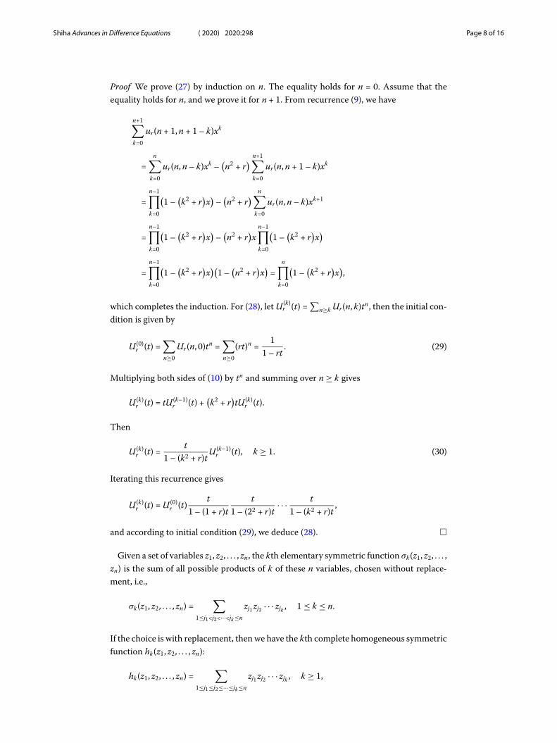
Proof We prove (27) by induction on n. The equality holds for n = 0. Assume that theequality holds for n, and we prove it for n + 1. From recurrence (9), we have

n+1∑

k=0

ur(n + 1, n + 1 – k)xk

=n∑

k=0

ur(n, n – k)xk –(n2 + r

) n+1∑

k=0

ur(n, n + 1 – k)xk

=n–1∏

k=0

(1 –

(k2 + r

)x)

–(n2 + r

) n∑

k=0

ur(n, n – k)xk+1

=n–1∏

k=0

(1 –

(k2 + r

)x)

–(n2 + r

)x

n–1∏

k=0

(1 –

(k2 + r

)x)

=n–1∏

k=0

(1 –

(k2 + r

)x)(

1 –(n2 + r

)x)

=n∏

k=0

(1 –

(k2 + r

)x),

which completes the induction. For (28), let U (k)r (t) =

∑n≥k Ur(n, k)tn, then the initial con-

dition is given by

U (0)r (t) =

∑

n≥0

Ur(n, 0)tn =∑

n≥0

(rt)n =1

1 – rt. (29)

Multiplying both sides of (10) by tn and summing over n ≥ k gives

U (k)r (t) = tU (k–1)

r (t) +(k2 + r

)tU (k)

r (t).

Then

U (k)r (t) =

t1 – (k2 + r)t

U (k–1)r (t), k ≥ 1. (30)

Iterating this recurrence gives

U (k)r (t) = U (0)

r (t)t

1 – (1 + r)tt

1 – (22 + r)t· · · t

1 – (k2 + r)t,

and according to initial condition (29), we deduce (28). �

Given a set of variables z1, z2, . . . , zn, the kth elementary symmetric function σk(z1, z2, . . . ,zn) is the sum of all possible products of k of these n variables, chosen without replace-ment, i.e.,

σk(z1, z2, . . . , zn) =∑

1≤j1<j2<···<jk≤n

zj1 zj2 · · · zjk , 1 ≤ k ≤ n.

If the choice is with replacement, then we have the kth complete homogeneous symmetricfunction hk(z1, z2, . . . , zn):

hk(z1, z2, . . . , zn) =∑

1≤j1≤j2≤···≤jk≤n

zj1 zj2 · · · zjk , k ≥ 1,


with initial conditions σ0(z1, z2, . . . , zn) = h0(z1, z2, . . . , zn) = 1. Note that σk(z1, z2, . . . , zn) = 0for k > n and hk(z1, z2, . . . , zn) �= 0 for k > n, for example h3(z1, z2) = z3

1 + z21z2 + z1z2

2 + z32. The

generating functions for σk and hk are given by

n∑

k=0

σk(z1, z2, . . . , zn)tk =n∏

i=1

(1 + zit), (31)

∑

k≥0

hk(z1, z2, . . . , zn)tk =n∏

i=1

(1 – zit)–1. (32)

From (27) and (28), we deduce that the numbers ur(n, k) and Ur(n, k) are the specializationsof the elementary and complete symmetric functions given by

ur(n, n – k) = (–1)kσk(r, 12 + r, 22 + r, . . . , (n – 1)2 + r

), (33)

Ur(n + k, n) = hk(r, 12 + r, 22 + r, . . . , n2 + r

). (34)

Recall that the central factorial numbers with even indices of both kinds satisfy

u(n, n – k) = (–1)kσk(12, 22, . . . , (n – 1)2), (35)

U(n + k, n) = hk(12, 22, . . . , n2). (36)

And the Stirling numbers of both kinds satisfy

s(n, n – k) = (–1)kσk(1, 2, . . . , n – 1), (37)

S(n + k, n) = hk(1, 2, . . . , n). (38)

Proposition 2 (Merca [23]) Let k and n be two positive integers, then

gk(z1 + t, z2 + t, . . . , zn + t) =k∑

i=0

(n – ci

k – i

)gi(z1, z2, . . . , zn)tk–i, (39)

where t, z1, z2, . . . , zn are variables, gi is any of these complete or elementary symmetric func-tions and

ci =

⎧⎨

⎩i, if gi = σi,

1 – k, if gi = hi.

In the next theorem, we show that the array ur(n, k) (Ur(n, k)) can be expressed in termsof u(n, k) (U(n, k)) and vice versa.

Theorem 6 If n, k, r ≥ 0, then

ur(n, k) =n∑

i=k

(ik

)u(n, i)(–r)i–k , (40)

u(n, k) =n∑

i=k

(ik

)ur(n, i)ri–k , (41)


Ur(n, k) =n∑

i=k

(ni

)U(i, k)rn–i, (42)

U(n, k) =n∑

i=k

(ni

)Ur(i, k)(–r)n–i. (43)

Proof To show (40), note that

ur(n, n – k) = (–1)kσk(r, 12 + r, 22 + r, . . . , (n – 1)2 + r

)

= (–1)kk∑

i=0

(n – ik – i

)σi

(0, 12, . . . , (n – 1)2)rk–i

=k∑

i=0

(n – ik – i

)(–1)iσi

(0, 12, . . . , (n – 1)2)(–r)k–i

=k∑

i=0

(n – ik – i

)u(n, n – i)(–r)k–i.

Then

ur(n, k) =n–k∑

i=0

(n – i

n – k – i

)u(n, n – i)(–r)n–k–i

=n∑

i=k

(i

i – k

)u(n, i)(–r)i–k .

For (42), note that

Ur(n + k, n) = hk(r, 12 + r, . . . , n2 + r

)

=k∑

i=0

(n + kk – i

)hi

(02, 12, . . . , n2)rk–i

=k∑

i=0

(n + kk – i

)U(n + i, n)rk–i.

Thus

Ur(n, n – k) =k∑

i=0

(n

k – i

)U(n – k + i, n – k)rk–i,

then we obtain

Ur(n, k) =n–k∑

i=0

(n

n – k – i

)U(k + i, k)rn–k–i =

n∑

i=k

(n

n – i

)U(i, k)rn–i.

The proofs of (41) and (43) are similar. �


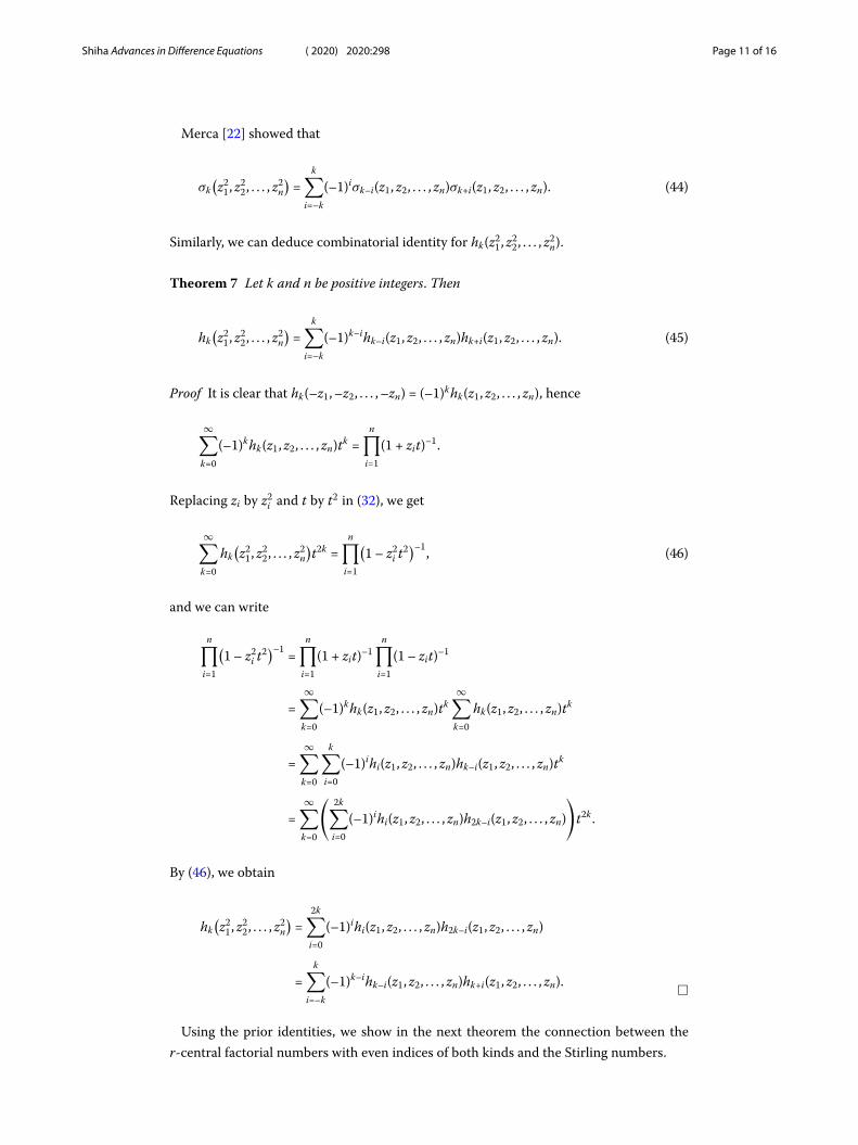
Merca [22] showed that

σk(z2

1, z22, . . . , z2

n)

=k∑

i=–k

(–1)iσk–i(z1, z2, . . . , zn)σk+i(z1, z2, . . . , zn). (44)

Similarly, we can deduce combinatorial identity for hk(z21, z2

2, . . . , z2n).

Theorem 7 Let k and n be positive integers. Then

hk(z2

1, z22, . . . , z2

n)

=k∑

i=–k

(–1)k–ihk–i(z1, z2, . . . , zn)hk+i(z1, z2, . . . , zn). (45)

Proof It is clear that hk(–z1, –z2, . . . , –zn) = (–1)khk(z1, z2, . . . , zn), hence

∞∑

k=0

(–1)khk(z1, z2, . . . , zn)tk =n∏

i=1

(1 + zit)–1.

Replacing zi by z2i and t by t2 in (32), we get

∞∑

k=0

hk(z2

1, z22, . . . , z2

n)t2k =

n∏

i=1

(1 – z2

i t2)–1, (46)

and we can write

n∏

i=1

(1 – z2

i t2)–1 =n∏

i=1

(1 + zit)–1n∏

i=1

(1 – zit)–1

=∞∑

k=0

(–1)khk(z1, z2, . . . , zn)tk∞∑

k=0

hk(z1, z2, . . . , zn)tk

=∞∑

k=0

k∑

i=0

(–1)ihi(z1, z2, . . . , zn)hk–i(z1, z2, . . . , zn)tk

=∞∑

k=0

( 2k∑

i=0

(–1)ihi(z1, z2, . . . , zn)h2k–i(z1, z2, . . . , zn)

)t2k .

By (46), we obtain

hk(z2

1, z22, . . . , z2

n)

=2k∑

i=0

(–1)ihi(z1, z2, . . . , zn)h2k–i(z1, z2, . . . , zn)

=k∑

i=–k

(–1)k–ihk–i(z1, z2, . . . , zn)hk+i(z1, z2, . . . , zn). �

Using the prior identities, we show in the next theorem the connection between ther-central factorial numbers with even indices of both kinds and the Stirling numbers.


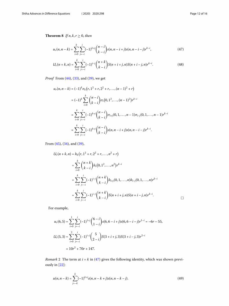
Theorem 8 If n, k, r ≥ 0, then

ur(n, n – k) =k∑

i=0

i∑

j=–i

(–1)k+j(

n – ik – i

)s(n, n – i + j)s(n, n – i – j)rk–i, (47)

Ur(n + k, n) =k∑

i=0

i∑

j=–i

(–1)i–j(

n + kk – i

)S(n + i + j, n)S(n + i – j, n)rk–i. (48)

Proof From (44), (33), and (39), we get

ur(n, n – k) = (–1)kσk(r, 12 + r, 22 + r, . . . , (n – 1)2 + r

)

= (–1)kk∑

i=0

(n – ik – i

)σi

(0, 12, . . . , (n – 1)2)rk–i

=k∑

i=0

i∑

j=–i

(–1)k+j(

n – ik – i

)σi+j(0, 1, . . . , n – 1)σi–j(0, 1, . . . , n – 1)rk–i

=k∑

i=0

i∑

j=–i

(–1)k+j(

n – ik – i

)s(n, n – i + j)s(n, n – i – j)rk–i.

From (45), (34), and (39),

Ur(n + k, n) = hk(r, 12 + r, 22 + r, . . . , n2 + r

)

=k∑

i=0

(n + kk – i

)hi

(0, 12, . . . , n2)rk–i

=k∑

i=0

i∑

j=–i

(–1)i–j(

n + kk – i

)hi+j(0, 1, . . . , n)hi–j(0, 1, . . . , n)rk–i

=k∑

i=0

i∑

j=–i

(–1)i–j(

n + kk – i

)S(n + i + j, n)S(n + i – j, n)rk–i.

�

For example,

ur(6, 5) =1∑

i=0

i∑

j=–i

(–1)1+j(

6 – i1 – i

)s(6, 6 – i + j)s(6, 6 – i – j)r1–i = –6r – 55,

Ur(5, 3) =2∑

i=0

i∑

j=–i

(–1)i–j(

52 – i

)S(3 + i + j, 3)S(3 + i – j, 3)r2–i

= 10r2 + 70r + 147.

Remark 2 The term at i = k in (47) gives the following identity, which was shown previ-ously in [22]:

u(n, n – k) =k∑

j=–k

(–1)k+js(n, n – k + j)s(n, n – k – j). (49)


And the term at i = k in (48) shows a new connection between U(n, k) and S(n, k):

U(n + k, n) =k∑

j=–k

(–1)k–jS(n + k + j, n)S(n + k – j, n). (50)

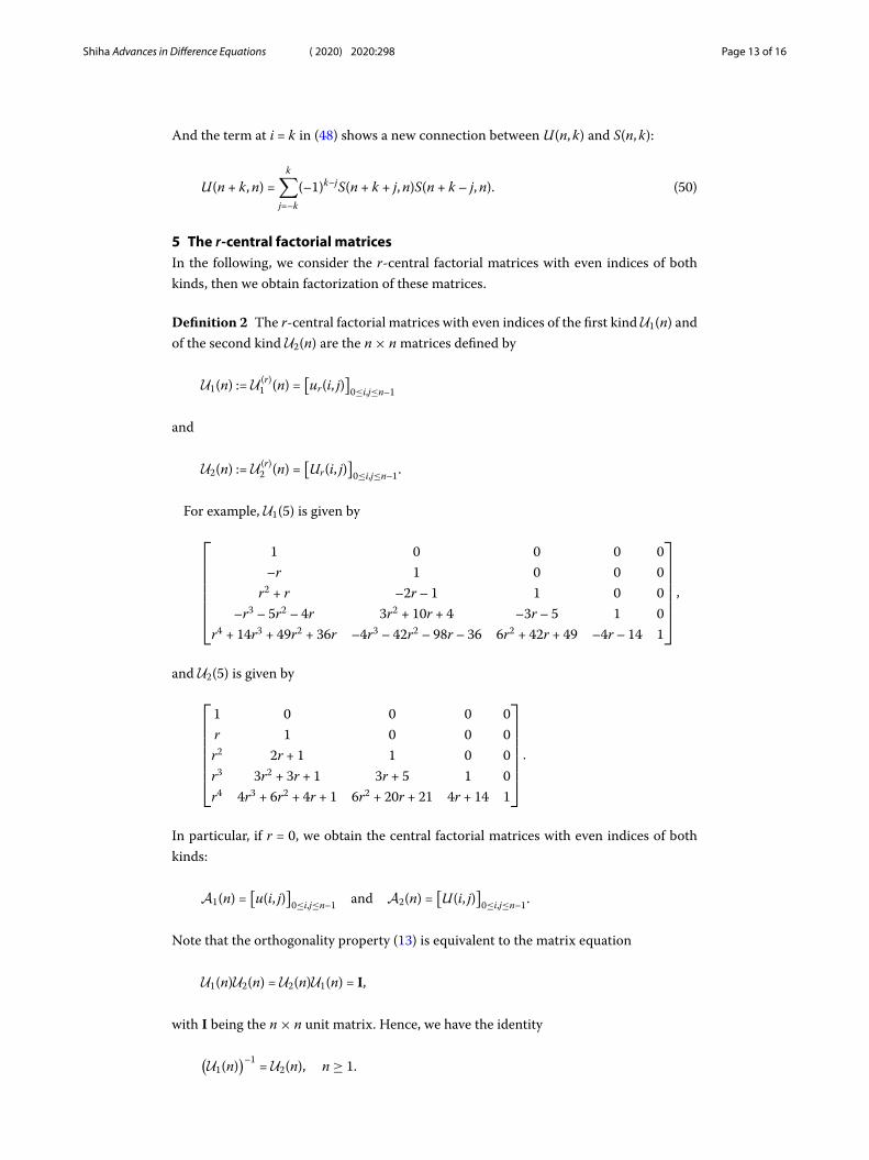
5 The r-central factorial matricesIn the following, we consider the r-central factorial matrices with even indices of bothkinds, then we obtain factorization of these matrices.

Definition 2 The r-central factorial matrices with even indices of the first kind U1(n) andof the second kind U2(n) are the n × n matrices defined by

U1(n) := U (r)1 (n) =

[ur(i, j)

]0≤i,j≤n–1

and

U2(n) := U (r)2 (n) =

[Ur(i, j)

]0≤i,j≤n–1.

For example, U1(5) is given by

⎡

⎢⎢⎢⎢⎢⎢⎣

1 0 0 0 0–r 1 0 0 0

r2 + r –2r – 1 1 0 0–r3 – 5r2 – 4r 3r2 + 10r + 4 –3r – 5 1 0

r4 + 14r3 + 49r2 + 36r –4r3 – 42r2 – 98r – 36 6r2 + 42r + 49 –4r – 14 1

⎤

⎥⎥⎥⎥⎥⎥⎦,

and U2(5) is given by

⎡

⎢⎢⎢⎢⎢⎢⎣

1 0 0 0 0r 1 0 0 0r2 2r + 1 1 0 0r3 3r2 + 3r + 1 3r + 5 1 0r4 4r3 + 6r2 + 4r + 1 6r2 + 20r + 21 4r + 14 1

⎤

⎥⎥⎥⎥⎥⎥⎦.

In particular, if r = 0, we obtain the central factorial matrices with even indices of bothkinds:

A1(n) =[u(i, j)

]0≤i,j≤n–1 and A2(n) =

[U(i, j)

]0≤i,j≤n–1.

Note that the orthogonality property (13) is equivalent to the matrix equation

U1(n)U2(n) = U2(n)U1(n) = I,

with I being the n × n unit matrix. Hence, we have the identity

(U1(n)

)–1 = U2(n), n ≥ 1.


In fact, inverse relations are known for practically all special numbers, such as Whitneynumbers and Stirling numbers (see [6, 7, 25, 26]).

Recall that the generalized n × n Pascal matrix Pn[z] is defined as follows (see [5]):

Pn[z] =[(

ij

)zi–j

]

0≤i,j≤n–1, (51)

with Pn = Pn[1], the Pascal matrix of order n. For example,

P5[z] =

⎡

⎢⎢⎢⎢⎢⎢⎣

1 0 0 0 0z 1 0 0 0z2 2z 1 0 0z3 3z2 3z 1 0z4 4z3 6z2 4z 1

⎤

⎥⎥⎥⎥⎥⎥⎦.

Moreover,

P–1n [z] = Pn[–z] =

[(–1)i–j

(ij

)zi–j

]

0≤i,j≤n–1.

From (40) and (42), we have the following factorization:

U1(n) = A1(n)Pn[–r], n ≥ 1, (52)

and

U2(n) = Pn[r]A2(n), n ≥ 1. (53)

For example,

U1(5) =

⎡

⎢⎢⎢⎢⎢⎢⎣

1 0 0 0 00 1 0 0 00 –1 1 0 00 4 –5 1 00 –36 49 –14 1

⎤

⎥⎥⎥⎥⎥⎥⎦×

⎡

⎢⎢⎢⎢⎢⎢⎣

1 0 0 0 0–r 1 0 0 0r2 –2r 1 0 0

–r3 3r2 –3r 1 0r4 –4r3 6r2 –4r 1

⎤

⎥⎥⎥⎥⎥⎥⎦

= A1(5)P5[–r]

and

U2(5) =

⎡

⎢⎢⎢⎢⎢⎢⎣

1 0 0 0 0r 1 0 0 0r2 2r 1 0 0r3 3r2 3r 1 0r4 4r3 6r2 4r 1

⎤

⎥⎥⎥⎥⎥⎥⎦×

⎡

⎢⎢⎢⎢⎢⎢⎣

1 0 0 0 00 1 0 0 00 1 1 0 00 1 5 1 00 1 21 14 1

⎤

⎥⎥⎥⎥⎥⎥⎦

= P5[r]A2(5).


6 ConclusionsIn this paper, we introduced the r-central factorial numbers with even indices of bothkinds as extended versions of the central factorial numbers with even indices of bothkinds. We derived the generating functions, some explicit expressions, and orthogonal-ity relations for such special numbers. In addition, we showed the relations between suchnumbers and the central factorial numbers with even indices which were also interpretedin matrix forms involving Pascal matrices. Also, we showed the relations between suchnumbers and the Stirling numbers. Finally, as an application to probability, we gave theprobability distribution of the unsigned r-central factorial numbers with even indices ofthe first kind.

AcknowledgementsThe author is deeply grateful to the editor and referees for their helpful comments in improving the presentation andquality of the paper.

FundingThere is no funding for this article.

Availability of data and materialsData sharing not applicable to this article as no data sets were generated or analysed during the current study.

Competing interestsThe author declares that she has no competing interests.

Authors’ contributionsThe author wrote the first version of the manuscript and approved the final manuscript by herself.

Publisher’s NoteSpringer Nature remains neutral with regard to jurisdictional claims in published maps and institutional affiliations.

Received: 26 February 2020 Accepted: 10 June 2020

References1. Acikgoz, M., Araci, S., Duran, U.: Some (p;q)-analogues of Apostol type numbers and polynomials. Acta Comment.

Univ. Tartu Math. 23(1), 37–50 (2019)2. Araci, S., Duran, U., Acikgoz, M.: On weighted q-Daehee polynomials with their applications. Indag. Math. 30, 365–374

(2019)3. Bóna, M.: Combinatorics of Permutations. Chapman & Hall/CRC, London (2004)4. Butzer, P.L., Schmidt, K., Stark, E.L., Vogt, L.: Central factorial numbers; their main properties and some applications.

Numer. Funct. Anal. Optim. 10(5&6), 419–488 (1989)5. Call, G.S., Velleman, D.J.: Pascal’s matrices. Am. Math. Mon. 100, 372–376 (1993)6. El-Desouky, B.S., Shiha, F.A.: A q-analogue of α-Whitney numbers. Appl. Anal. Discrete Math. 12, 178–191 (2018)7. El-Desouky, B.S., Shiha, F.A., Shokr, E.M.: The multiparameter r-Whitney numbers. Filomat 33(3), 931–943 (2019)8. Gelineau, Y., Zeng, J.: Combinatorial interpretations of the Jacobi–Stirling numbers. Electron. J. Comb. 17, R70 (2010)9. Hardy, G.H., Littlewood, J.E., Pólya, G.: Inequalities. Cambridge University Press, Cambridge (1959)10. Jang, L.-C., Kim, T., Kim, D.S., Kim, H.Y.: Extended r-central Bell polynomials with umbral calculus viewpoint. Adv. Differ.

Equ. 2019, 202 (2019)11. Khan, N., Usman, T., Choi, J.: A new class of generalized polynomials associated with Laguerre and Bernoulli

polynomials. Turk. J. Math. 43, 486–497 (2019)12. Kim, D.S., Dolgy, D.V., Kim, D., Kim, T.: Some identities on r-central factorial numbers and r-central Bell polynomials.

Adv. Differ. Equ. 2019, 245 (2019)13. Kim, D.S., Dolgy, D.V., Kim, T., Kim, D.: Extended degenerate r-central factorial numbers of the second kind and

extended degenerate r-central Bell polynomials. Symmetry 11(4), Article ID 595 (2019)14. Kim, D.S., Kim, H.Y., Kim, D., Kim, T.: On r-central incomplete and complete Bell polynomials. Symmetry 11(5), Article ID

724 (2019)15. Kim, T., Jang, L.-C., Kim, D.S., Kim, H.Y.: Some identities on type 2 degenerate Bernoulli polynomials of the second kind.

Symmetry 12(4), Article ID 510 (2020)16. Kim, T., Kim, D.S.: A note on central Bell numbers and polynomials. Russ. J. Math. Phys. 27(1), 76–81 (2020)17. Kim, T., Kim, D.S.: Degenerate polyexponential functions and degenerate Bell polynomials. J. Math. Anal. Appl. 487(2),

124017 (2020)18. Kim, T., Kim, D.S.: Some identities of extended degenerate r-central Bell polynomials arising from umbral calculus.

Rev. R. Acad. Cienc. Exactas Fís. Nat., Ser. A Mat. 114(1), Paper No. 1, 19 pp. (2020)19. Kim, T., Kim, D.S., Jang, G.-W.: On central complete and incomplete Bell polynomials I. Symmetry 11(2), Article ID 288

(2019)


20. Kim, T., Kim, D.S., Jang, G.-W., Kwon, J.: Extended central factorial polynomials of the second kind. Adv. Differ. Equ.2019, 24 (2019)

21. Kwon, J., Kim, T., Kim, D.S., Kim, H.Y.: Some identities for degenerate complete and incomplete r-Bell polynomials.J. Inequal. Appl. 2020, 23 (2020)

22. Merca, M.: A special case of the generalized Girard–Waring formula. J. Integer Seq. 15, Article 12.5.7 (2012)23. Merca, M.: A note on the r-Whitney numbers of Dowling lattices. C. R. Acad. Sci. Paris, Ser. I 351, 649–655 (2013)24. Merca, M.: Connections between central factorial numbers and Bernoulli polynomials. Period. Math. Hung. 73(2),

259–264 (2016)25. Mezö, I., Ramírez, J.L.: The linear algebra of the r-Whitney matrices. Integral Transforms Spec. Funct. 26(3), 213–225

(2015)26. Riordan, J.: Combinatorial Identities. Wiley, New York (1968)27. Samuels, S.M.: On the number of successes in independent trials. Ann. Math. Stat. 36(4), 1272–1278 (1965)28. Shattuck, M.: Generalizations of Bell number formulas of Spivey and Mezö. Filomat 30(10), 2683–2694 (2016)29. Stirling, J.: Methodus differentialis: sive Tractatus de Summatione et Interpolatione Serierum Inifinitarum. London

(1730)30. Wilf, H.S.: Generating Functionology. Academic Press/Harcourt Brace Jovanovich (1994)

the r-central factorial numbers with even indices

Documents