The Ramses Code for Numerical Astrophysics: Toward Full GPU Enabling

Claudio Gheller (ETH Zurich - CSCS)

Giacomo Rosilho de Souza (EPF Lausanne)

Marco Sutti (EPF Lausanne)

Romain Teyssier (University of Zurich)

•  Numerical simulations represent an extraordinary tool to study and solve astrophysical problems

•  They are actual virtual laboratories, where numerical experiments can run

•  Sophisticated codes are used to run the simulations on the

most powerful HPC systems

Simulations in astrophyisics

2

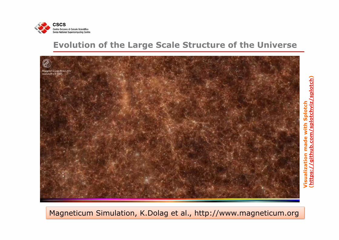
Evolution of the Large Scale Structure of the Universe

Vis

ual

izat

ion

mad

e w

ith

Sp

lotc

h

(htt

ps:

//

git

hu

b.c

om/

splo

tch

viz/

splo

tch

)

Magneticum Simulation, K.Dolag et al., http://www.magneticum.org

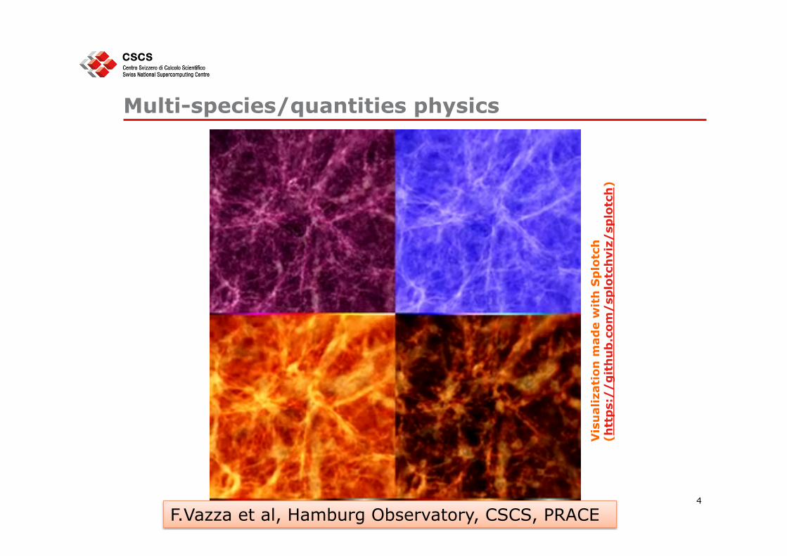
Multi-species/quantities physics

4

Vis

ual

izat

ion

mad

e w

ith

Sp

lotc

h

(htt

ps:

//

git

hu

b.c

om/

splo

tch

viz/

splo

tch

)

F.Vazza et al, Hamburg Observatory, CSCS, PRACE

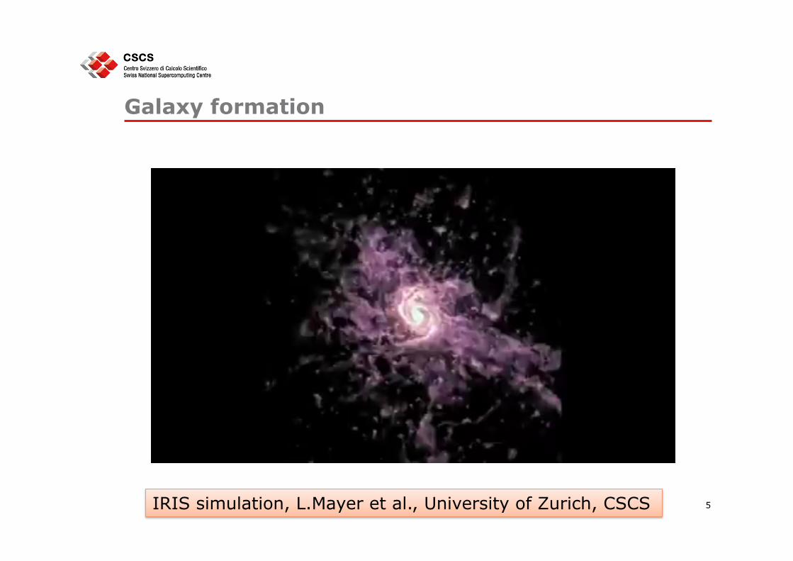
Galaxy formation

5 IRIS simulation, L.Mayer et al., University of Zurich, CSCS

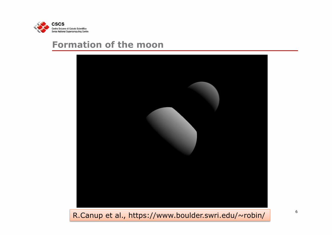
Formation of the moon

6 R.Canup et al., https://www.boulder.swri.edu/~robin/

Codes: RAMSES

•  RAMSES (R.Teyssier, A&A, 385, 2002): code to study of astrophysical problems

•  various components (dark energy, dark matter, baryonic matter, photons) treated

•  Includes a variety of physical processes (gravity, magnetohydrodynamics, chemical reactions, star formation, supernova and AGN feedback, etc.)

•  Adaptive Mesh Refinement adopted to provide high spatial resolution ONLY where this is strictly necessary

•  Open Source •  Fortran 90 •  Code size: about 70000 lines •  MPI parallel (public version) •  OpenMP support (restricted access) •  OpenACC under development

HPC power: Piz Daint

8

“Piz Daint” CRAY XC30 system @ CSCS (N.6 in Top500) Nodes: 5272 CPUs 8-core Intel SandyBridge equipped with: •  32 GB DDR3 memory •  One NVIDIA Tesla K20X GPU with 6 GB of GDDR5 memory

Overall system •  42176 cores and 5272 GPUs •  170+32 TB •  Interconnect: Aries routing and communications ASIC, and

dragonfly network topology •  Peak performance: 7.787 Petaflops

Scope

Overall goal: Enable the RAMSES code to exploit hybrid, accelerated architectures

9

Adopted programming model: OpenACC (http://www.openacc-standard.org/) Development follows an incremental “bottom-up” approach

RAMSES: modular physics

AMR build Load Balance Gravity

Hydro

N-Body

Tim

e lo

op

MHD

Cooling RT More Physics

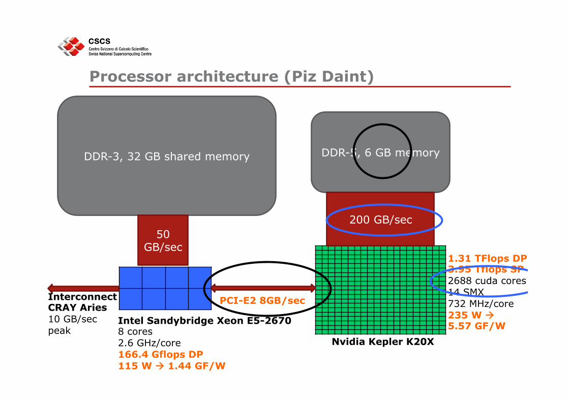
DDR-3, 32 GB shared memory DDR-5, 6 GB memory

PCI-E2 8GB/sec

Nvidia Kepler K20X

200 GB/sec 50

GB/sec 1.31 TFlops DP 3.95 Tflops SP 2688 cuda cores 14 SMX 732 MHz/core 235 W à 5.57 GF/W

Interconnect CRAY Aries 10 GB/sec peak

Intel Sandybridge Xeon E5-2670 8 cores 2.6 GHz/core 166.4 Gflops DP 115 W à 1.44 GF/W

Processor architecture (Piz Daint)

RAMSES: Modular, incremental GPU implementation

AMR build Load Balance Gravity

Hydro

N-Body

MPI

Tim

e lo

op MHD

MPI

Cooling RT More Physics

MPI

Low GF

Mid GF

Hi GF

Mid GF Hi GF

GF = “GPU FRIENDLY” Computational intensity + Data independency

First steps toward the GPU

AMR build Load Balance Gravity

Hydro

N-Body

MPI

Tim

e lo

op MHD

MPI

Cooling RT More Physics

MPI

Low GF

Mid GF

Hi GF

Mid GF Hi GF

GF = “GPU FRIENDLY” Computational intensity + Data independency

Step 1: solving fluid dynamics

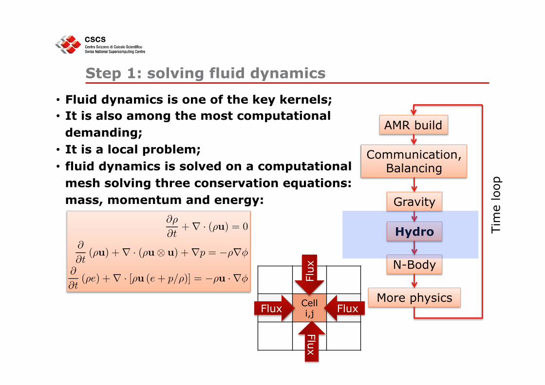
•  Fluid dynamics is one of the key kernels; •  It is also among the most computational

demanding; •  It is a local problem; •  fluid dynamics is solved on a computational

mesh solving three conservation equations: mass, momentum and energy:

Cell i,j Flux Flux

Flux

Flux

AMR build

Communication, Balancing

Gravity

Hydro

N-Body

More physics

Tim

e lo

op

6 R. Teyssier: Cosmological Hydrodynamics with Adaptive Mesh Refinement

whose cloud is entirely included within the level bound-ary are concerned. For particles belonging to level ℓ, butwhose cloud lies partially outside the level volume, the ac-celeration is interpolated from the mesh of level ℓ−1. Thisis the same for the ART code: “In this way, particles aredriven by the coarse force until they move sufficiently farinto the finer mesh” (Kravtsov et al. 1997).

2.2.5. Time integration

One requirement in a coupled N-body and hydrodynami-cal code is the possibility to deal with variable time steps.The stability conditions for the time step is indeed givenby the Courant Friedrich Levy (CFL) condition, whichcan vary in time. The standard leapfrog scheme (Hockney& Eastwood 1981), though accurate, does not offer thispossibility. In RAMSES, a second-order midpoint schemehas been implemented, which reduces exactly to the sec-ond order leapfrog scheme for constant time steps. Sincethe acceleration −∇φn is known at time tn from particlepositions xn

p , positions and velocities are updated first bya predictor step

vn+1/2p = vn

p −∇φn∆tn/2 (5)

xn+1p = xn

p + vn+1/2p ∆tn (6)

and then by a corrector step

vn+1p = vn+1/2

p −∇φn+1∆tn/2 (7)

In this last equation, the acceleration at time tn+1 isneeded. In order to avoid an extra call to the Poissonsolver, this last operation is postponed to the next timestep. The new velocity is computed as soon as the newpotential is obtained. In RAMSES, it is possible to haveeither a single time step for all particles, or individual timesteps for each level. In the latter case, when a particle exitslevel ℓ with time step ∆tℓ, the corrector step is applied atlevel ℓ−1, using ∆tℓ in place of ∆tℓ−1. Therefore, the “pasthistory” of all particles has to be known in order to applycorrectly the corrector step. This is done in RAMSES byintroducing one extra integer per particle indicating itscurrent level. This particle “color” is eventually modifiedat the end of the corrector step.

Usually, the time step evolution is smooth, making ourintegration scheme second-order in time. However, if oneuses the adaptive time step scheme instead of the more ac-curate (but time consuming) single time step scheme, thetime step changes abruptly by a factor of two for particlescrossing a refinement boundary. Only first order accuracyis retained along those particle trajectories. This loss ofaccuracy has been analyzed in realistic cosmological con-ditions (Kravtsov & Klypin 1999; Yahagi & Yoshii 2001)and turns out to have a small effect on the particle distri-bution, when compared to the single time step case.

2.3. Hydrodynamical Solver

In RAMSES, the Euler equations are solved in their con-servative form:

∂ρ

∂t+ ∇ · (ρu) = 0 (8)

∂

∂t(ρu) + ∇ · (ρu⊗ u) + ∇p = −ρ∇φ (9)

∂

∂t(ρe) + ∇ · [ρu (e + p/ρ)] = −ρu ·∇φ (10)

where ρ is the mass density, u is the fluid velocity, e is thespecific total energy, and p is the thermal pressure, with

p = (γ − 1)ρ(e −1

2u2) (11)

Note that the energy equation (Eq. 10) is conservativefor the total fluid energy, if one ignores the source termsdue to gravity. This property is one of the main advan-tages of solving the Euler equations in conservative form:no energy sink due to numerical errors can alter the flowdynamics. Gravity is included in the system of equationas a non stiff source term. In this case, the system is notexplicitly conservative and the total energy (potential +kinetic) is conserved at the percent level (see section 4.3).

Let Uni denote a numerical approximation to the cell-

averaged value of (ρ, ρu, ρe) at time tn and for cell i. Thenumerical discretization of the Euler equations with grav-itational source terms writes:

Un+1i − Un

i

∆t+

Fn+1/2i+1/2 − Fn+1/2

i−1/2

∆x= Sn+1/2

i (12)

The time centered fluxes Fn+1/2i+1/2 across cell interfaces are

computed using a second-order Godunov method (alsoknown as Pieceweise Linear Method), with or without di-rectional splitting (according to the user’s choice), whilegravitational source terms are included using a time cen-tered, fractional step approach:

Sn+1/2i =

!

0,ρn

i ∇φni + ρn+1

i ∇φn+1i

2,(ρu)n

i ∇φni + (ρu)n+1

i ∇φn+1i

2

"

(13)

A general description of Godunov and fractional stepmethods can be found in Toro (1997). The present im-plementation is based on the work of Collela (1990) andSaltzman (1994). For sake of brevity, only its basic fea-tures are recalled here.

2.3.1. Single grid Godunov solver

In this section, I describe the basic hydrodynamicalscheme used in RAMSES to solve equations (8-10) at agiven level. It is assumed that proper boundary conditionshave been provided: the hydrodynamical scheme requires2 ghost zones in each side and in each direction, even inthe diagonal directions. Since in RAMSES the Euler equa-tions are solved on octs of 2dim cells each, 3dim− 1 similarneighboring octs are required to define proper boundaryconditions. The basic stencil of the PLM scheme therefore

The challenge: RAMSES AMR Mesh

Fully Threaded Tree with Cartesian mesh •  CELL BY CELL refinement •  COMPLEX data structure •  IRREGULAR memory distribution

GPU implementation of the Hydro kernel 1.   Memory Bandwidth:

1.  reorganization of memory in spatially (and memory) contiguous large patches, so that work can be easily split in blocks with efficient memory access

2.  Further grouping of patches to increase data locality 2.   Parallelism:

1.  patches to blocks assignment, 2.  one cell per thread integration

3.   Data transfer: 1.  Offload data only when and where necessary

4.   GPU memory size: 1.  Still an open issue…

Some Results: hydro only

17

Fraction of time saved using the GPU

Scalability of the CPU and GPU versions (Total time)

Scalability of the CPU and GPU versions (Hydro time)

•  Data movement is still 30-40% overhead: can be worse with more complex AMR hierarchies

•  A large fraction of the code is still on the CPU

•  No overlap of GPU and CPU computation

We need to extend the fraction of the code enabled to the GPU, reducing data transfers and overlapping as much as possible to the remaining CPU part

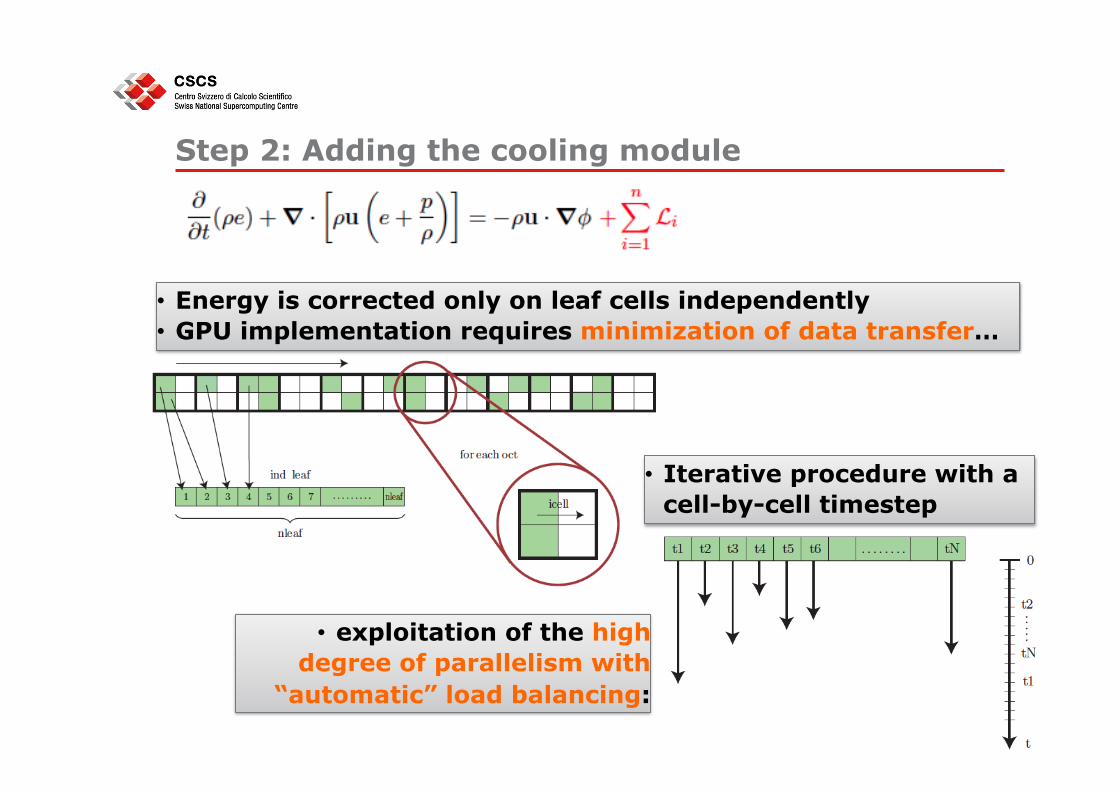
Step 2: Adding the cooling module

•  Energy is corrected only on leaf cells independently •  GPU implementation requires minimization of data transfer…

•  exploitation of the high degree of parallelism with

“automatic” load balancing:

•  Iterative procedure with a cell-by-cell timestep

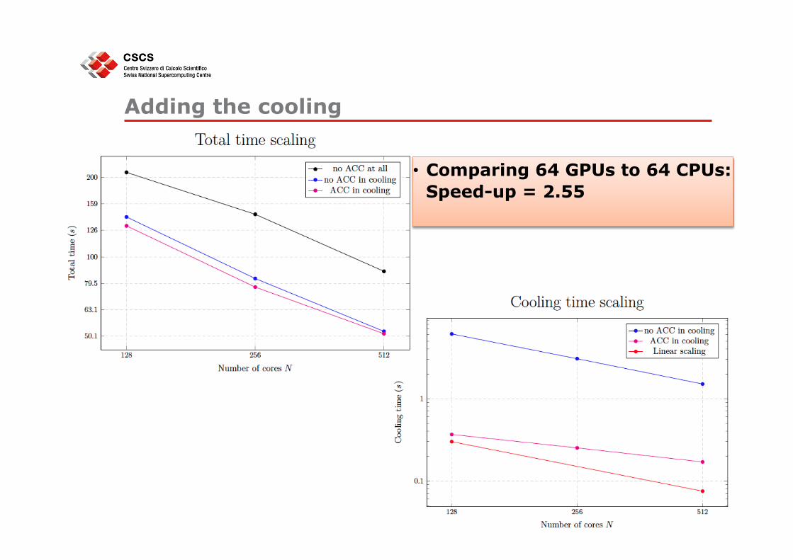
Adding the cooling

19

•  Comparing 64 GPUs to 64 CPUs: Speed-up = 2.55

Toward a full GPU enabling

20

•  Gravity is being moved to the GPU

•  ALL MPI communication is being moved to the GPU using the GPUDirect MPI implementation

•  N-body will stay on the CPU •  Low computational intensity •  Can easily overlap to the GPU •  No need of transferring all particle data, saving time but

especially GPU memory

Summary Objective: Enable the RAMSES code to the GPU Methodology Incremental approach exploiting RAMSES’modular architecture and OpenACC programming mode Current achievement: Hydro and Cooling kernels ported on GPU; MHD kernel almost done On-going work: •  Move all MPI stuff to the GPU •  Enable gravity to the GPU •  Data transfer minimization

21

Thanks for your attention

22