The rank of a product of two matrices X and Y is equal to the smallest of the rank of X and Y:

Rank (X Y) =min (rank (X) , rank (Y))

0

0.05

0.1

0.15

0.2

0.25

0.3

0.35

0.4

400 450 500 550 600Wavelength (nm)

Ab

so

rba

nc

e

0

0.5

1

1.5

2

2.5

0 2 4 6 8 10 12

Time (s)

Co

nc

en

tra

tio

n

A = CS

Eigenvectors and EigenvaluesFor a symmetric, real matrix, R, an eigenvector v is obtained from:

Rv = v is an unknown scalar-the eigenvalue

Rv – v= 0 (R – Iv= 0The vector v is orthogonal to all of the row

vector of matrix (R-I)

R v = v

0v- R I =

0.1 0.2 0.3

0.2 0.4 0.6A= R=ATA =

0.14 0.28

0.28 0.56

Rv = v(R – Iv= 00.14 0.28

0.28 0.56

1 0

0 1-

v1

v2

0

0=

=0.14 - 0.28

0.28 0.56 - =0

0

v1

v2

0

0

0.14 0.28

0.28 0.56-

v1

v2

(0.14 – ) (0.56 – ) – (0.28) (0.28) = 0

= 0

= 0

&

0.14 - 0.28

0.28 0.56 - = 0

For

=0

0

0.14 – 0.28

0.28 0.56 –

v11

v21

-0.56 0.28

0.28 -0.14=

v11

v21

-0.56 v11 + 0.28v21 = 0

0.28 v11 - 0.14 v21 = 0

v21 = 2 v11

Normalized vector v1 =0.4472

0.8944

If v11 = 1 v21 = 2

0.14 0.28

0.28 0.56=

0

0

v12

v22

0.14 v12 + 0.28 v22 = 0

0.28 v12 +0.56 v22 = 0

v12 = -2 v22

If v22 = 1 v12 = -2

Normalized vector v1 =-0.8944

0.4472

For

0.1 0.2 0.3

0.2 0.4 0.6A=

Rv = vRV = V

V =-0.8944

0.4472

0.4472

0.8944

0.7 0

0 0v1v2 =0

R=ATA =0.14 0.28

0.28 0.56

More generally, if R (p x p) is symmetric of rank r≤p then R posses r positive eigenvalues and (p-r) zero eigenvalues

tr(R) = i= 0.7 + 0.0 =0.7∑

Example

Consider 15 sample each contain 3 absorbing components

?

Show that in the presence of random noise the number of non-zero eigenvalues is larger than numbers of components

Variance-Covariance Matrix

x11 – mx1

…

x21 – mx1

(xn1 – mx1)

x12 – mx2

x22 – mx2

xn2 – mx2

…

…

…

…

…

x1p – mxp

x1p – mxp

xnp – mxp

…X =

Column mean centered matrix

XTX =

var(x1)

… ……

…

…

… …

var(x2)

var(xp)

covar(x1x2) covar(x1xp)

covar(x2x1) covar(x2xp)

covar(xpx1) covar(xpx2)

mmcn.m file for mean centering a matrix

?

Use anal.m file and mmcn.m file and verify that each eigenvalue of an absorbance data matrix is correlated with variance of data

Singular Value DecompositionSVD of a rectangular matrix X is a method which yield at the same time a diagnal matrix of singular values S and the two matrices of singular vectors U and V such that :

X = U S VT UTU = VTV =Ir

The singular vectors in U and V are identical to eigenvectors of XXT AND XTX, respectively and the singular values are equal to the positive square roots of the corresponding eigenvalues

X = U S VT XT = V S UT

X XT= U S VT VSUT= US2UT

(X XT) U = US2

=

X = U S VT = s1u1v1T + … + srurvr

T

X

m

n

U

m

n

S

n

n

VT

n

n

If the rank of matrix X=r then;

X

m

n

= U

m

r

Sr

r

VT

r

n

Singular value decomposition with MATLAB

Consider 15 sample containing 2 component with strong spectral overlapping and construct their absorbance data matrix accompany with random noise

Ideal data

A

Noised data

nd

Reconstructed data

rd

residual

R1

Ideal data

Aresidual

R2

- =

- =

It can be shown that the reconstructed data matrix is closer to ideal data matrix

Anal.m file for constructing the data matrix

Spectral overlapping of two absorbing species

Ideal data matrix A

Noised data matrix, nd, with 0.005 normal distributed random noise

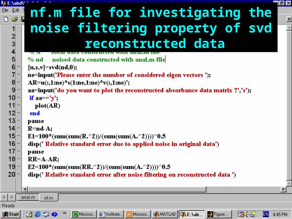
nf.m file for investigating the noise filtering property of svd reconstructed data

?

Plot the %relative standard error as a function of number of eigenvectors

x11 x12 x114

x21 x21 x214…

…

Principal Component Analysis (PCA)

• • • • • • • • • • • • • •

x1

x2

PCA

• • • • • • • • • • • • • •

u 1

u 2

u11

u12

u114

…

•

• ••

••

• •• •

•• ••

x1

x2

x11 x12 x114

x21 x21 x214…

…

•

• ••

••

• •• •

•• •• u 1u 2 u11

u12

u114

…

u21

u22

u214

…

Principal Components in two Dimensions

u1 = ax1 + bx2

u2 = cx1 + dx2

0.10.2

0.20.4

0.30.6

1 2 s1

s2

s3

In principal components model new variables are found which give a clear picture of the variability of the data. This is best achieved by giving the first new variable maximum variance, the second new variable is then selected so as to be uncorrelated with the first one, and so on

The new variables can be uncorrelated if:

ac + bd =0a=1 b=2 c=-1 d=0.5

0.1

0.2

0.3

x1 =

0.2

0.4

0.6

x2 =

0.5

1.0

1.5

u1 = var(u1)=0.25

a=2 b=4 c=-2 d=1

1.0

2.0

3.0

u1 = var(u1)=1.0

Orthogonality constraint

Normalizing constraint a2 + b2 = 1c2 + d2 = 1

a=1 b=2

c=-1 d=0.5

a=0.4472 b=0.8944

c=-0.8944 d=0.4472

Normalizing

a=2 b=4

c=-2 d=1Normalizing a=0.4472 b=0.8944

c=-0.8944 d=0.4472

Maximum variance constraint

u1 = ax1 + bx2

2u1 = a2 2

x1 + b2 2x2 + 2ab x1-x2

2u1 = [ a b ]

2x1 x1-x2

x1-x2 2x2

a

b

= 2u1

2x1 x1-x2

x1-x2 2x2

a

b

a

b

Principal Components in m Dimensionsx11 x12 … x1m

x21 x22 … x2m

xn1 xn2 … xnm

…

…

… X=

u1 = v11x1 + v12x2 + … + v1mxm

u2 = v21x1 + v22x2 + … + v2mxm

um = vm1x1 + vm2x2 + … + vmmxm

…

…

…

…

var(x1)… …

…

…

…

… …

var(x2)

var(xm)

covar(x1x2) covar(x1xm)

covar(x2x1) covar(x2xm)

covar(xmx1) covar(xmx2)

v11

v21

vm1

…

var(u1)=

v11

v21

vm1

…

C V V=

Xn

m m

m

V Un

m

=

X V =U

Xn

m m

m

V Un

m

=

Loading vectors Score vectors

X VTV = UVT

VT V = I X = UVT = S LT

Xn

m

sn

mm

m

LT=

X = USVT S = US

More generally, when one analyzes a data matrix consisting of n objects for which m variables have been determined, m principal components can then be extracted (as long as m<n.

PC1 represents the direction in the data containing the largest variation. PC2 is orthogonal to PC1 and represents the direction of the largest residual variation around PC1. PC3 is orthogonal to the first two and represents the direction of the highest residual variation around the plane formed by PC1 and PC2.

PCA.m file

10 mixtures of two componentsanal.m file

?

Perform PCA on data matrix obtained from an evolutionary process, such as kinetic data (kin.m file) and interpret the score vectors.

Classification with PCA

The most informative view of a data set, in terms of variance at least, will be given by consideration of the first two PCs. Since the scores matrix contains a value for each sample corresponding to each PC, it is possible to plot these values against one another to produce a low dimensional picture of a high-dimensional data set.

Suppose there are 20 sample from two different class

0

0.05

0.1

0.15

0.2

0.25

0.3

400 450 500 550 600

Wavelength (nm)

Ab

so

rba

nc

e Class I Class II

0

0.04

0.08

0.12

0.16

400 450 500 550 600

Wavelength (nm)

Ab

so

rba

nc

e

0

0.02

0.04

0.06

0.08

0.1

0.12

0 0.05 0.1 0.15

Abs. (1)

Ab

s. (

2)

0

0.025

0.05

0.075

0.1

0.125

0.15

400 450 500 550 600Wavelength (nm)

Ab

so

rba

nc

e

00.02

0.040.06

0.080.1

0.120.14

0.16

0 0.05 0.1 0.15Abs. ( 1)

Ab

s. (

2)

0

0.05

0.1

0.15

0.2

0.25

0.3

400 450 500 550 600Wavelength (nm)

Ab

so

rba

nc

e Class I Class II

-0.12-0.1

-0.08-0.06-0.04-0.02

00.020.040.060.080.1

-0.8 -0.6 -0.4 -0.2 0

PC1

PC

2

Multiple Linear Regression (MLR)

y = b1 x1 + b2 x2 + … + bp xp

x11 …

x21

xn1

x12

x22

xn2

…

……

……

x1p

x2p

xnp…

b1

b2

bp

…

y1

y2

yn

… =y = X b

= y

n

1

X

n

p

b1

p

If p>n

a1 = 1 c11 + 2 c12 + 3 c13

a2 = 1 c21 + 2 c22 + 3 c23

There is an infinite number of solution for , which all fit the equation

If p=n

a1 = 1 c11 + 2 c12 + 3 c13

a2 = 1 c21 + 2 c22 + 3 c23

a3 = 1 c31 + 2 c32 + 3 c33

It gives a unique solution for provided that the X matrix has ful rank

If p<n

y1 = 1 c11 + 2 c12 + 3 c13

a2 = 1 c21 + 2 c22 + 3 c23

a3 = 1 c31 + 2 c32 + 3 c33

a4= 1 c41 + 2 c42 + 3 c43

This does not allow an exact solution for , but one can get a solution by minimizing the length of the residual vector eThe least squares solution is

= (CTC)-1 CT a

Least Squares in Matrix Equations

= y

n

1

X

n

p

y = X b

y

n

1

= x1

n

1

x2

n

1

xp

n

1

b111

bp11

b211

+ + … +

For solving this system the Xb-y must be perpendicular to the column space of X

1

pb

Suppose vector Xc is a linear combination of the columns of X :

(Xc)T [Xb – y]=0

c [XTXb –XT y]=0XTXb = XT y

b = (XTX)-1 XT yThe projection of y onto the column space of X is therefore

p=Xb = (X (XTX)-1 XT )y

Least Squares Solution

Projection the y vector in column space of X

The error vector

The error vector is perpendicular to all columns of X matrix

MLR with more than one dependent variable

= y1

n

1

X

n

p 1

pb1y3

n

1

y2

n

1 1

pb2

1

pb3

=Y

n

m

X

n

p

Bp

m

Y= X B B= (XTX) -1 Y

Classical Least Squares (CLS)A= C K

=A

n

m

C

n

p

Kp

m

Calibration step K = (CTC)-1 CT AThe number of calibration standards should at least be as large as the number of analytesThe rank of C must be equal to p

Prediction step aTun= cT

un K cun= (KKT)-1 K aun

Number of wavelengths mustbe equal or larger than number of components

Advantages of CLSFull spectral domain is used for estimating each constituent. Using redundant information has an effect equivalent to replicated measurement and signal averaging, hence it improves the precision of the concentration estimates.

Disadvantages of CLSThe concentration of all the constituents in the calibration set have to be known

Simultaneous determination of two

components with CLS

Random design of concentration matrix

Pure component spectra

Absorbance data matrix

Data matrices for mlr.m file

mlr.m file for multiple linear regression

Predicted concentrations

Real concentrations

?

Use CLS method for determination of one component in binary mixture samples

Inverse Least Squares (ILS)c= A b

Calibration step b = (ATA)-1 AT c1

The number of calibration samples should at least be as large as the number of wavelengthsThe rank of A must be equal to p

Prediction step cTun= aT

un b

= c1

n

1

A

n

p 1

pb

Advantages of ILSIt is not necessary to know all the information on possible constituents, analyte of interest and interferents

Disadvantages of ILS

The number of calibration samples should at least be as large as the number of wavelengths

The method can work in principal when unknown chemical interferents are present. It is important that such interferents are present in calibration samples

Determination of x in the presence of y by ILS

method

15 x 9 absorbance data matrix

ILS.m file

ILS calibration

Predicted concentrationsReal concentrations

?

Does in ILS method the accuracy of final results is dependent to number of wavelength?

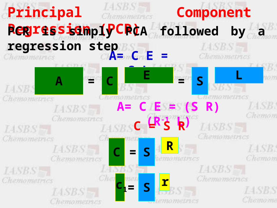
Principal Component Regression (PCR)PCR is simply PCA followed by a regression step

A= C E = S L

A C E= S L=

A= C E = (S R) (R-1 L)

C = S R

C S R=

S r=c1

A data matrix can be represented by its score matrixA regression of score matrix against one or several dependent variables is possible, provided that scores corresponding to small eigenvalues are omittedThis regression gives no matrix inversion problemPCR has the full-spectrum advantages of the CLS methodPCR has the ILS advantage of being able to perform the analysis one chemical components at a time while avoiding the ILS wavelength selection problem

ValidationHow many meaningful principal components should be retained?

*Percentage of explained variance

If all possible PCs are used in the model 100% of the variance is explained

sd2 =

∑ ii=1

d

∑ ii=1

p x 100

Percentage of explained variance for determination of number of PCs

Spectra of 20 samples of various amount of 2 components

Pev.m file for

percentage of explained variance method

Performing pev.m file on nd absorbance data matrix

?

Show the validity of results of Percentage Explained Variance method is dependent to spectral overlapping of individual components

A

n

p

loading

n

p

n

n

score

PCA

A

n

p

A’

n-1

p

cp

1 a

Cross-Validation

Creating absorbance data for performing cross-validation

method

Spectra of 15 samples of various amount of 3 components

cross.m file for

PCR cross-validation

PCR cross-validation

01234567

0 5 10 15

no of factors

PR

ES

Scross-validation plot

c = S b

Calibration and Prediction Steps in PCR

=c1

n

1

Sn

r

br

1

b = ( STS)-1 ST c

Calibration Step

Axm

p

L

p

rr

mSx =

Prediction StepSx = Ax L

cx = Sx b

Pcr.m file for calibration and prediction by PCR method

Spectra of 20 samples of various amount of 3 components

Input data for pcr.m file

pcr.m function

Predicted and real values for first component

Predicted and real values for first component

Predicted and real values for first component

?

Compare the CLS, ILS and PCR methods for prediction in a two components system with strong spectral overlapping