The RaPId Toolbox for Parameter Identification and Model ValidationHow Modelica and FMI helped to create something nearly impossible in the electrical power systems field!

Prof.Dr.-Ing. Luigi Vanfretti

luigiv@kth.se Associate Professor, Docent

School of Electrical EngineeringKTH

Stockholm, Sweden

Luigi.Vanfretti@statnett.noSpecial Advisor in Strategy and

International CollaborationResearch and Development Division

Statnett SFOslo, Norway

E-mail: luigiv@kth.se, luigi.vanfretti@statnett.no Web: http://www.vanfretti.com

FMI Tech Day – Volvo Cars TorslandaMarch 11, 2015 - Gothenburg, Sweden

Outline• Background:

– Modeling and simulation of large scale power systems– What is iTesla and where is Modelica used?

• Why Model Validation in Power Systems?– Motivation– Overview of WP3 tasks in iTesla

• Unambiguous power system modeling and simulation using Modelica-Driven Tools– Limitations of current modeling approaches used in power systems– iTesla Power Systems Modelica Library

• Mock-up SW prototype for model validation:– Model validation software architecture based using Modelica tools and FMI

Technologies– Prototype proof-of-concept implementation: the Rapid Parameter Identification

Toolbox (RaPId) – Sample applications

• Conclussions

Acknowledgment

• The work presented here is a result of the collaboration between RTE (France), AIA (Spain) and KTH (Sweden) within the EU funded FP7 iTesla project: http://www.itesla-project.eu/

• The following people have contributed to this work:

– RTE: Patrick Panciatici, Jean-Baptiste Hyberger, Angela Chieh– AIA: Gladys De Leon, Milenko Halat, Marc Sabate– KTH: Wei Li, Tetiana Bogodorova, Maxime Baudette, Jan Lavenius, Francisco Gomez

Lopez, Achour Amazouz, Joan Russiñol, Mengjia Zhang, Janelle (Le) Qi … and others!

• Special thanks for ‘special training’ and support from– Prof. Fritzson and his team at Linköping University– Prof. Berhard Bachmann and Lennart Ochel, FH Bielefeld

UNAMBIGUOUS POWER SYSTEM MODELING AND SIMULATION USING MODELICA TOOLS

Modeling and Simulation

5

• They are those who help bring power for you to charge your iPhone, ;-)• … and they are hard to operate – when things fail, its expensive: e.g. European “blackout”

ocurred on 4/11/2006• The frequency drops to 49 Hz, which causes automatic load schedding.• Real power surplus of 6000 MW

Electrical Power Systems? What are those?

Large Scale Power SystemsTo operate large power networks, planners and operators need to analyze variety of operating conditions – both off-line and in near real-time (power system security assessment).

Different SW systems have been designed for this purpose.

But, the dimension and complexity of the problems are increasing due to growth in electricity demand, lack of investments in transmission, and penetration of intermittent resources.

New tools are needed!

Current/new tools will need to perform simulations:• Of complex hybrid model components and networks with

very large number of continuous and discrete states.• Models need to be shared, and simulation results need

to be consistent across different tools and simulation platforms…

• If models could be “systematically shared at the equation level”, and simulations are “consistent across different SW platforms” – we would still need to validate each new model (new components) and calibrate the model to match reality.

Power system dynamics

10-7 10-6 10-5 10-4 10-3 10-2 10-1 1 10 102 103 104

Lightning

Line switching

SubSynchronous Resonances, transformer energizations…

Transient stability

Long term dynamics

Daily load following

seconds

Electromechanical Transients

Electromagnetic Transients

Quasi-Steady State Dynamics

Phasor Time-Domain Simulation

Power System Dynamics in Europe February 19th 2011

49.85

49.9

49.95

50

50.05

50.1

50.15

08:08:00 08:08:10 08:08:20 08:08:30 08:08:40 08:08:50 08:09:00 08:09:10 08:09:20 08:09:30 08:09:40 08:09:50 08:10:00

f [H

z]

20110219_0755-0825

Freq. Mettlen Freq. Brindisi Freq. Wien Freq. Kassoe

Synchornized Phasor Measurement Data

Power System Phasor-Time Domain Modeling and Simulation Status Quo

10-7 10-6 10-5 10-4 10-3 10-2 10-1 1 10 102 103 104

Lightning

Line switching

SubSynchronous Resonances, transformer energizations…

Transient stability

Long term dynamics

Daily load following

seconds

Phasor Time-Domain Simulation

PSS/EStatus Quo:Multiple simulation tools, with their own interpretation of different model features and data “format”.Implications of the Status Quo:- Dynamic models can rarely be shared in a

straightforward manner without loss of information on power system dynamics (parameter not equal to equations, block diagrams not equal to equations)!

- Simulations are inconsistent without drastic and specialized human intervention.

Beyond general descriptions and parameter values, a common and unified modeling language would require a formal mathematical description of the models – but this is not the practice to date.

These are key drawbacks of today’s tools for tackling pan-European problems.

Common Architecture of « most » Available Power System Security Assessment Tools

Online

Data acquisition and storage

Merging module

Contingency screening (static power flow)

Synthesis of recommendations for the operator

External data (forecasts and

snapshots)

“Static power flow model”

That means no (dynamic) time-domain simulation is performed.

The idea is to predict the future behavior under a given ‘contingency’ or set of contingencies.

BUT, the model has no dynamics – only nonlinear algebraic equations.

Computations made on the power system model are based on a “power flow” formulation.

Result : difficult to predict the impact of a contingency without considering system dynamics!

iTesla Toolbox ArchitectureOnline Offline

Sampling of stochastic variables

Elaboration of starting network

states

Impact Analysis (time domain simulations)

Data mining on the results of

simulation

Data acquisition and storage

Merging module

Contingency screening (several stages)

Time domain simulations

Computation of security rules

Synthesis of recommendations for the operator

External data (forecasts and

snapshots)

Improvements of defence and

restoration plans

Offline validation of dynamic models

Focus of this presentation

Where are Models used?

Sampling of stochastic variables

Elaboration of starting network

states

Impact Analysis (time domain simulations)

Data mining on the results of

simulation

Data acquisition and storage

Merging module

Contingency screening (several stages)

Time domain simulations

Computation of security rules

Synthesis of recommendations for the operator

External data (forecasts and

snapshots)

Improvements of defence and

restoration plans

Offline validation of dynamic models

Data management

Data mining services

Dynamic simulation Optimizers Graphical

interfaces

Modelica use planned for time-domain simulation:

Developing a builder/translator using the iTesla Internal Data Model (IIDM)

WHY POWER SYSTEM MODEL VALIDATION?

Motivation

Why “Model Validation”?• iTesla tools aim to perform

“security assessment”• The quality of the models

used by off-line and on-line tools will affect the result of any SA computations

– Good model: approximates the simulated response as “close” to the “measured response” as possible

• Validating models helps in having a model with “good sanity” and “reasonable accuracy”:

– Increasing the capability of reproducing actual power system behavior (better predictions)

2 3 4 5 6 7 8 9-2

-1.5

-1

-0.5

0

0.5

1

P

(pu

)

Time (sec)

Measured Response

Model Response

US WECC Break-up in 1996

BAD Model for Dynamic Security Assessment!!!

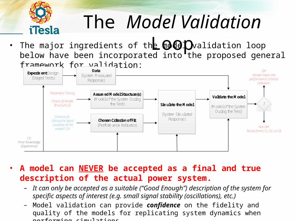
The Model Validation Loop• The major ingredients of the model validation loop below have been

incorporated into the proposed general framework for validation:

• A model can NEVER be accepted as a final and true description of the actual power system.

– It can only be accepted as a suitable (“Good Enough”) description of the system for specific aspects of interest (e.g. small signal stability (oscillations), etc.)

– Model validation can provide confidence on the fidelity and quality of the models for replicating system dynamics when performing simulations.

– Calibrated models will be needed for systems with more and more dynamic interactions

(1)Prior Knowledge

(Experience)

Parameter Tuning

Choice of Model Structure (2)

Criterion fit:- fitting the data?- purpose of the

model? (3)

OK!Model meets the

performance criteria/indicator.

Not OK!Revise from (1), (2), or (3)

Experiment Design(Staged Tests)

Data(System Measured

Response)

Assumed Model Structure(s)(Model of the System During

the Test) Simulate the Model

(System Simulated Response)Chosen Criterion of Fit

(Performance Indicator)

Validate the Model

(Model of the System During the Test)

?

Different Validation Levels

• Component level– e.g. generator such as wind

turbine or PV panel

• Cluster level– e.g. gen. cluster such as wind

or PV farm

• System level– e.g. power system small-signal

dynamics (oscillations)

G1

G2

G3

G4

G5

G7

G6

G8

G9

Overview of Model Validation work in iTesla

Parameter Estimation using

measurements and high bandwidth

simulated responses

Validated Device Models

Methods for the Assessment of large-

power network simulation responses

against measurements

Methods to Generate Aggregate

Models of PV and Wind Farms

Validated Aggregate Models

Tasks on Device Model Validation and Parameter

Estimation

Tasks on Methods to Obtain Aggregate Models

and their Validation

Tasks on Large-Power System Model Dynamic Performance

Assessment

WP3Off-line validation of dyanmic models

Dynamic performance

discrepancy indexes

Synchronized Phasor Measurements and high bandwidth model simulated responses

Requ

irem

ents

fo

r Val

idati

on Limitations of com

mon m

odeling practices

Task on Validation

Requirements

Task on Identification of modeling limitations

of current practices

Validated Models and Model Parameters,

Updated Models, and Discrepancy Indexes

Unvalidated Models, Models that need updates, Etc.

WP2Data Needs, Collection and Management

Func

tiona

l Sp

ecifi

catio

n of

W

P6 T

ools

Task 3.1

Task 3.2

Task 3.3

Task 3.4

Task 3.5

UNAMBIGUOUS POWER SYSTEM MODELING AND SIMULATION USING MODELICA-DRIVEN TOOLS

Modeling and Simulation

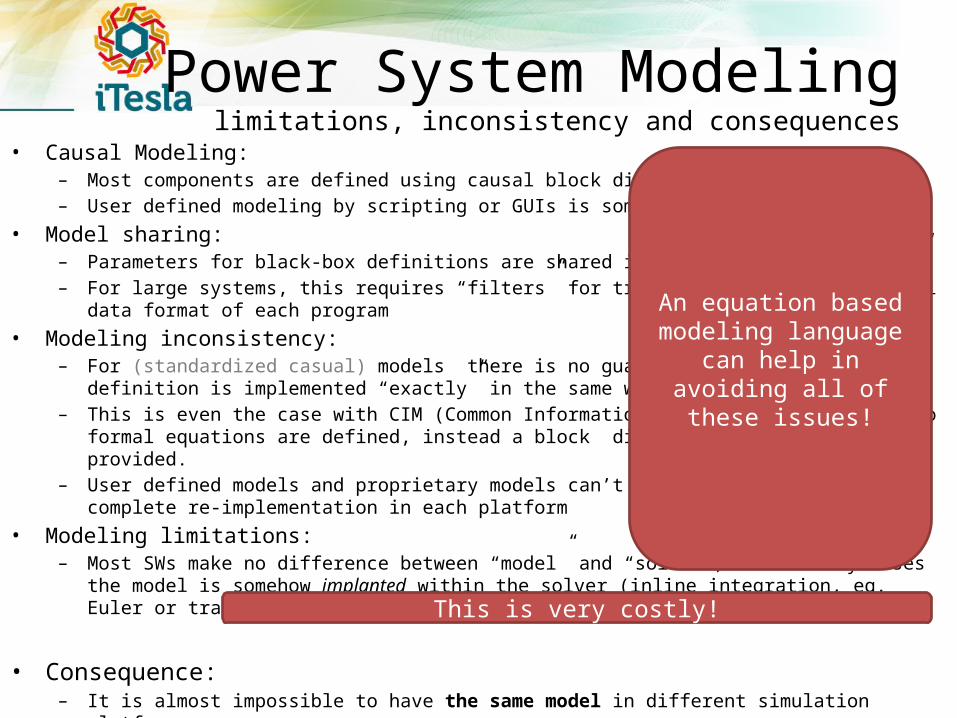
Power System Modelinglimitations, inconsistency and consequences

• Causal Modeling:– Most components are defined using causal block diagram definitions.– User defined modeling by scripting or GUIs is sometimes available (casual)

• Model sharing:– Parameters for black-box definitions are shared in a specific “data format”– For large systems, this requires “filters” for translation into the internal data format of each program

• Modeling inconsistency:– For (standardized casual) models there is no guarantee that the model definition is implemented “exactly” in the

same way in different SW– This is even the case with CIM (Common Information Model) dynamics, where no formal equations are defined,

instead a block diagram definition is provided.– User defined models and proprietary models can’t be represented without complete re-implementation in each

platform• Modeling limitations:

– Most SWs make no difference between “model” and “solver”, and in many cases the model is somehow implanted within the solver (inline integration, eg. Euler or trapezoidal solution in transient stability simulation)

• Consequence: – It is almost impossible to have the same model in different simulation platforms.– This requires usually to re-implement the whole model from scratch (or parts of it) or to spend a lot of time “re-

tuning” parameters.

This is very costly!

An equation based modeling language can help in avoiding all of

these issues!

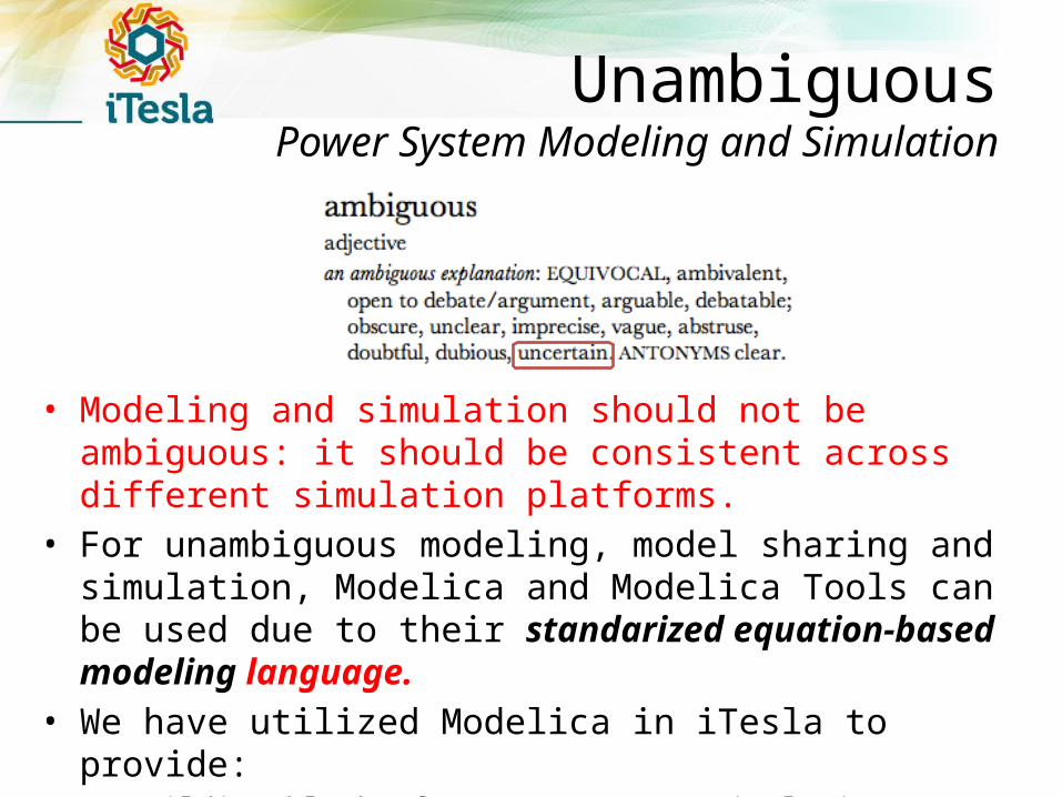
• Modeling and simulation should not be ambiguous: it should be consistent across different simulation platforms.

• For unambiguous modeling, model sharing and simulation, Modelica and Modelica Tools can be used due to their standarized equation-based modeling language.

• We have utilized Modelica in iTesla to provide:– Building blocks for power system simulation: iTelsa PS Modelica Library– The possibility to use FMUs for model sharing in general purpose tools

and exploiting generic solvers

UnambiguousPower System Modeling and Simulation

iTesla Power Systems Modelica Library

• Power Systems Library:– The Power Systems library developed using as reference domain specific software tools

(e.g. PSS/E, Eurostag, PSAT and others)• PSS/E and Eurostag (proprietary) , PSAT (OSS) power system specific simulation tools.

– The library has been tested in several Modelica supporting software: OpenModelica, Dymola, SystemModeler and Jmodelica.org.

– Components and systems are validated against the proprietary tools and OSS tool

• New components and time-driven events are being added to this library in order to simulate new systems.

– PSS/E (proprietary tool) equivalents of different components are now available and being validated.

– Automatic translator from domain specific tools to Modelica will use this library’s classes to build specific power system network models is being developed.

iTesla Power Systems Modelica Library in OpenModelica

SW-to-SW Validation ofModels used by TSOs

• Derive the equations– Eletrocmagnetic dynamics– Motion– Saturation– Stator voltage equations

• Boundary equations – Change coordinate

• Provide initial (guess) values for the initialization problem

Validation of a PSS/E Model: Genrou

Typical SW-to-SW Validation Tests

• Basic grid

• Perturbation scenarios

• Set-up a model in each tool with the simulation scenario configured

• In the case of Modelica, the simulation configuration can be done within the model

• In the case of PSS/E, a Python script is created to perform the same test.

• Sample Test:1. Running under steady state for 2s.2. Vary the system load with constant P/Q ratio.3. After 0.1s later, the load was restored to its original value .4. Run simulation to 10s.5. Apply three phase to ground fault.6. 0.15s later clear fault by tripping the line.7. Run simulation until 20s.

Model Set-Up of SW-to-SWValidation Tests

Modelica

PSS/E

Python

Results from Validation Testfor GENROU

ITESLA MODEL VALIDATION MOCK-UP SOFTWARE PROTOTYPE

RaPId: a proof of concept implementation using Modelica and FMI Technologies

What is required from a SW architecture for model validation?

Models

Static Model

Standard Models

Custom Models

Manufacturer Models

System LevelModel Validation

Measurements

Static Measurements

Dynamic Measurements

PMU Measurements

DFR Measurements

Other

Measurement, Model and Scenario

Harmonization

Dynamic Model

SCADA MeasurementsOther EMS Measurements

Static Values:- Time Stamp- Average Measurement Values of P, Q and V- Sampled every 5-10 sec

Time Series:- GPS Time Stamped Measurements- Time-stamped voltage and current phasor meas.

Time Series with single time stamp:- Time-stamp in the initial sample, use of sampling frequency to determine the time-stamp of other points- Three phase (ABC), voltage and current measurements- Other measurements available: frequency, harmonics, THD, etc.

Time Series from other devices (FNET FDRs or Similar):- GPS Time Stamped Measurements- Single phase voltage phasor measurement, frequency, etc.

Scenario

Initialization

State Estimator Snap-shop

DynamicSimulation

Limited visibility of custom or manufacturer models will by itself put a limitation on the methodologies used for model validation

• Support “harmonized” dynamic models

• Process measurements using different DSP techniques

• Perform simulation of the model

• Provide optimization facilities for estimating and calibrating model parameters

• Provide user interaction

User Target(server/pc)

Model Validation Software

iTesla WP2 Inputs to WP3: Measurements & Models

Mockup SW ArchitectureProof of concept of using MATLAB+FMI

EMTP-RV and/or other HB model simulation traces and simulation configuration

PMU and other available HB measurements

SCADA/EMS Snapshots + Operator Actions

MAT

LAB

MATLAB/Simulink (used for simulation of the Modelica Model in FMU format)

FMI Toolbox for MATLAB(with Modelica model)

Model Validation Tasks:

Parameter tuning, model optimization, etc.

User Interaction

.mat and

.xml files

HARMONIZED MODELICA MODEL:Modelica Dynamic Model Definition for Phasor Time Domain Simulation

Data Conditioning

iTesla Cloud or Local Toolbox

Installation

Internet or LAN.mo files

.mat and

.xml files

FMU compiled by another tool

FMU

Proof-of-Concept Implementation of the iTesla Model Validation SW Mock-Up Prototype

• RaPId is our proof of concept implementation • RaPId is meant for use in WP3.3 and WP3.4 used

for Component Parameter Estimation and Aggregate Model Parameter Estimation and Validation

• RaPId is a toolbox providing a framework for parameter identification.

• Based on Modelica and FMI – applicable to other systems, not only power systems!

• A Modelica model, made available through a Flexible Mock-Unit (i.e. FMU) in the Simulink environment, is characterized by a certain number of parameters whose values can be independently chosen.

• The model is simulated and its outputs are compared against measurements.

• RaPId attempts to tune the parameters of the model in so as to satisfy a fitness criterion (e.g. minimize the error between the simulation and measurement traces) between the outputs of the Simulation and the experimental measurements of the same outputs provided by the user.

RaPId Interface

Options and

Settings

Algorithm Choice

Results and Plots

Simulink Containerl

Output measurement data

Input measurement data

• RAPID has been developed in MATLAB, where the MATLAB code acts as wrapper to provide interaction with several other programs.

• Advanced users can simply use MATLAB scripts instead of the interface.

• Plug-in Architecture:– Completely extensible and open

architecture allows advanced users to add:

• Identification methods• Optimization methods• Specific objective functions• Solvers (integration

routines)

What does RaPId do?

1 Output (and optionally input) measurements are provided to RaPId by the user.

2 At initialization, a set of parameter is generated randomly or preconfigured in RaPId.

3 The model is simulated with the parameter values given by RaPId.

4 The outputs of the model are recorded and compared to the user-provided measurements.

5 A fitness function is computed to judge how close the measured data and simulated data are to each other

Based on the fitness computed in (5) a new set of parameters is computed by RaPId 2’

1

2

3

4

5

2’

The simulations continue until a minimal fitness or a maximum number of iterations (simulation runs) are reached.

File Structure

RaPId gui

core

GUI - Contains the configuration menus, and the main window.

algos

functions algoFunctions

rapidFunctions

Functions adapting the calls to the optimization method to the parameter optimization of RaPId

Functions used by the algorithm implemented with the toolbox (pso, ga, naive method)

Base functions of the toolbox

Data files use to transfer data from the GUI to rRaPId. Can be read by the user after computation.

Modelica, Examples, Experiments

Directories containing Modelica and FMU models, Examples, Experiments, other…

Implementationrapid.m

Called from the GUI or the command line, needs to be fed the settings struct and the measured data

Reads in settings the name of the method to be used, call the appropriate method

xxx_algo.m

func.m

Rapid_simuSystem.m

Rapid_objectiveFunction.m

Generates iteratively parameter vectors to test taking into account past values of the parameters and corresponding fitness (example of methods: PSO, GA, Gradient) stop after a number of iterations or when a condition on fitness is reached Provide a vector of parameter,

expect the fitness as return value

Simulate the simulink model with the vector of parameters fed by the method and return the output of the model

Evaluate the fitness of the vector of parameters based on the output from the simulation and the output measuredSeveral criterions can be used

Return the fitness

Functions from : \core\functions\rapidFunctions

Plugins: Obj. Functions

function fitness = rapid_objectiveFunction( realRes, simuRes,settings) %OBJECTIVEFUNCTION compute the fitness criterion % Default - quadratic criterion % realRes is data used for matching, from measurments % simuRes is the data we want to have matching realRes % the two of them are under the shape [[x[1];y[1]] [x[2];y[2]] ... [x[nStep];y[nStep]]] % % settings has to contain the fields % cost: integer, for quadratic cost the value is 2 % objective: struct adapted to the method chose % if cost = 2, objective contains the field: % Q: nb_parameters*nb_parameters weight matrix, % should take into account the respective outputs scaling switch settings.cost case 2 nStep = size(realRes,2); nx = size(settings.objective.Q,1); Q_ = repmat({settings.objective.Q},1,nStep); Q_ = blkdiag(Q_{:}); fitness = (realRes(:)-simuRes(:))'*Q_*(realRes(:)-simuRes(:)); otherwise errorWrongCost end end

rapid_objectiveFunction, choose a keyword: eg. case 2.

To plugin a new optimization function: add a case to the switch, in the body of the case, compute the fitness of the vector of parameters based on realRes and simuRes, (measured and simulated output signals).

realRes is an interpolation of the result of the simulation at the time instants given by the measurement data. Allows to compare measured and simulated data point to point.

A new method can be added for fitness computation if the appropriate keyword is given in settings.cost

You can define as many elements as needed inside settings.objective, in the example here a weight matrix is provided in settings.objective

Here the fitness is characterised by one unique matrix Q :

Plugins:Optim. Methods (1)

function [ sol, historic ] = rapid( settings, systemDescription ) %RAPID main function of the rapid toolbox RaPId global nbIterations nbIterations = 0; % Set-up the simulink model to run between 0 and tf with a step of Ts and % with the solver given by settings.methodName, the function % rapid_simuSystem call the simulation in the workspace of rapid.m after % changing the parameters value through fmuSetValueSimulink addpath(settings.rapidFolder); settings.realData = rapid_interpolate(systemDescription,settings); % choose and launch the desired method for parameter estimation switch settings.methodName case 'pso' [ sol, historic, settings ] = pso_algo(settings); case 'ga' [ sol, historic, settings ] = ga_algo(settings); case 'naive' sol = naive_algo(settings); historic = []; case 'cg' [ sol, historic, settings ] = cg_algo(settings); case 'nm' [ sol, historic, settings ] = nm_algo(settings); case 'combi' settings2 = settings; settings2.methodName = settings2.combiOptions.firstMethod; [sol1,historic1, settings2] = rapid(settings2,systemDescription); settings2.methodName = settings2.combiOptions.secondMethod; settings2.p0 = sol1; [sol,historic2, settings] = rapid(settings2,systemDescription); historic.sol1 = sol1; historic.historic1 = historic1; historic.historic2 = historic2; case 'psoExt' [ sol, historic, settings ] = psoExt_algo(settings); case 'gaExt' [ sol, historic, settings ] = gaExt_algo(settings); otherwise errorWrongMethodName end end

A case with a new keyword in the function rapid.m can be added.

Call your method methodName_algo.

It takes the struct settings as argument and return the vector solution.

A new method can only call the function func(v) func takes a vector of parameter and returns the fitness associated to this vector.

This assumes that the good settings.cost and settings.objective were declared to use the objective function you desire to evaluate.

func takes care of simulating the model, saving its output, interpolating the output data and computing the fitness.

All fields of the settings struct must however be filled correctly. (Not presented here)

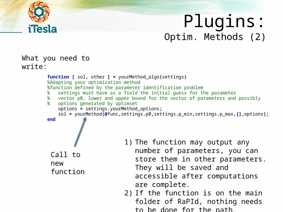
function [ sol, other ] = yourMethod_algo(settings) %Adapting your optimization method %function defined by the parameter identification problem % settings must have as a field the initial guess for the parameter % vector p0, lower and upper bound for the vector of parameters and possibly % options generated by optimset options = settings.yourMethod_options; sol = yourMethod(@func,settings.p0,settings.p_min,settings.p_max,[],options); end

What you need to write:

Call to new function

1) The function may output any number of parameters, you can store them in other parameters. They will be saved and accessible after computations are complete.

2) If the function is on the main folder of RaPId, nothing needs to be done for the path management.

Plugins:Optim. Methods (2)

Using RaPId forfor parameter estimation

• The objective is to determine which vector of parameters gives the best fit on the output

• The parameterized model of this system is written in Modelica and imported into the MATLAB/Simulink environment using the FMI Toolbox for Matlab

• RaPId is excecuted times (simulation/excecution runs) until the performance indicator is acceptable.

𝑦 (𝑡)𝑢(𝑡 )System studied

System to be identified

S(θ)

𝑢(𝑡 ) 𝑦 (𝑡)

θ𝑖

A Textbook Example: Measurement-based parameter identification of an “unknown” component

Assume we have the measured response of a system, subject to a change in the input where is a vector of unknown parameters to be identified.

We now hypothesize that the model of the unknown component can be posed as a transfer function of the form

The Modelica model for can be easily built.

The parameters , and are calibrated be minimizing the error between measured and simulated response with the fitness function:

Measurement

• We use an initial guess of the parameters of the model (un-calibrated parameters): = [0.4, 4.15, 1.75 ,1.15]

• After the optimization process, the parameters obtained by RaPId, which satisfy the performance indicator are:

= [0.3413, 4.5488, 1.7956, 1.1374]• Observe that the true model is given indeed by a transfer function with

parameters: = [0.3, 4.00, 1.6 ,1.00]

• To obtain the exact parameters, the performance indicator needs to be stricter – leading to more executions of the calibration process.

Measurements

Model response with initial guess

Demo!

simout

To Workspace

Scope

datameasured

FromWorkspace

y1

FMUrafael

FMU of the Modelica Model in the Simulink Container

Measurements from tests are imported into MATLAB:

Δοκιμή 1/ 60% MCR/-200 mHz/ 900sec.

220

230

240

250

260

270

280

19

:58

:11

19

:58

:58

19

:59

:45

20

:00

:32

20

:01

:19

20

:02

:06

20

:02

:53

20

:03

:40

20

:04

:27

20

:05

:14

20

:06

:01

20

:06

:48

20

:07

:35

20

:08

:22

20

:09

:09

20

:09

:56

20

:10

:43

20

:11

:30

20

:12

:17

20

:13

:04

20

:13

:51

20

:14

:38

20

:15

:25

20

:16

:12

20

:16

:59

Ώρα

Ισχύ

ς

99.5

99.6

99.7

99.8

99.9

100

100.1

Συχ

νότη

τα (%

) ως

πο

σο

τό τ

ων

50H

z

Pow er output(MW)

InjectedSignal (%)

*Rescaling to p.u. was performed after data extraction.

Application ExampleModel Parameter Identification for a Greek Generating Plant

iGrGen ModelFMU in Simulink

for RaPId

Algorithms: PF vs. PSOParticle Filter PSO

Assumption: The Particle Filter approach will reduce the solution space to samples that will result in a lower values of the fitness function (lower error).In contrast, PSO will have slower convergence as it will evaluate the fitness function over the whole solution space, for each iteration.

Results of identification

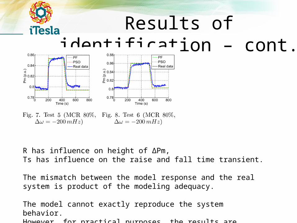
Results of identification – cont.

R has influence on height of ΔPm,Ts has influence on the raise and fall time transient.

The mismatch between the model response and the real system is product of the modeling adequacy. The model cannot exactly reproduce the system behavior.However, for practical purposes, the results are satisfactory.

Results using PF and PSO

The assumption on faster convergence of the Particle Filter over PSO appears to be valid from the results above.

Conclusions andLooking Forward

• Modeling power system components with Modelica (as compared with domain specific tools) is very attractive:– Formal mathematical description of the model (equations)– Allows model exchange between Modelica tools, with consistent

(unambiguous) simulation results• The FMI Standard allows to take advantage of Modelica models for:

– Using Modelica models in different simulation environments– Coupling general purpose tools to the model/simulation (case of RaPId)

• There are several challenges for modeling and validated “large scale” power systems:– A well populated library of typical components (and for different time-scales)– Model builder from domain-specific tools “data files/base” (in development)– Support/linkage with industry specific data exchange paradigm (Common

Information Model - CIM)• Developing a Modelica-driven model validation for large scale power systems will

prove more complex challenge than the case of RaPId.

Questions?

luigiv@kth.se luigi.vanfretti@statnett.no

Thank you!

50