the rasch rating model and -...

Educational and PsychologicalMeasurement

72(4) 547–573� The Author(s) 2012

Reprints and permission:sagepub.com/journalsPermissions.nav

DOI: 10.1177/0013164411432166http://epm.sagepub.com

The Rasch Rating Model andthe Disordered ThresholdControversy

Raymond J. Adams1, Margaret L. Wu2, and Mark Wilson3

Abstract

The Rasch rating (or partial credit) model is a widely applied item response modelthat is used to model ordinal observed variables that are assumed to collectivelyreflect a common latent variable. In the application of the model there is consider-able controversy surrounding the assessment of fit. This controversy is most notablewhen the set of parameters that are associated with the categories of an item haveestimates that are not ordered in value in the same order as the categories. Someconsider this disordering to be inconsistent with the intended order of the responsecategories in a variable and often term it reversed deltas. This article examines a vari-ety of derivations of the model to illuminate the controversy. The examination of thederivations shows that the so-called parameter disorder and order of the responsecategories are separate phenomena. When the data fit the Rasch rating model theresponse categories are ordered regardless of the (order of the) values of the para-meter estimates. In summary, reversed deltas are not necessarily evidence of a prob-lem. In fact the reversed deltas phenomenon is indicative of specific patterns in therelative numbers of respondents in each category. When there are preferences aboutsuch relative numbers in categories, the patterns of deltas may be a useful diagnostic.

Keywords

partial credit model, Rasch model, Rasch rating model

1Australian Council for Educational Research, Melbourne, and University of Melbourne, Parkville, Victoria,

Australia2Victoria University, Melbourne, Victoria, Australia3University of California, Berkeley, Berkeley, CA, USA

Corresponding Author:

Raymond J. Adams, University of Melbourne, 234 Queensberry St. Parkville 3054, Victoria, Australia

Email: [email protected]

The Rasch rating (or partial credit) model (Andrich, 1978; Masters, 1982) is a widely

applied item response model that is used to model ordinal variables that are assumed

to collectively reflect a common latent variable.

In the application of the model there is considerable controversy in relation to the

practical implications of situations where the set of parameters that are associated

with the categories of an item have estimates that are not ordered in value. Some con-

sider this phenomenon to be inconsistent with the intended order of the response cate-

gories in a variable and often term it either disordered thresholds or reversed deltas.

The view that estimated parameter disorder represents an incompatibility of the

data with the underlying measurement intentions of Rasch measurement has been

strongly advocated by Andrich (1978, 2005) and is embodied in Andrich’s computer

program, RUMM2020 (Andrich, Sheridan, & Luo, 2003), which routinely alerts users

to this as a problem. Furthermore, in a number of applied settings disorder of esti-

mated parameters has been used as evidence of a problem with the intended ordering

of the response categories (e.g., Nijsten, Sampogna, Chren, & Abeni, 2006; Nilsson,

Sunnerhagen, & Grimby, 2007; Zhu, Timm, & Ainsworth, 2001).

Other model and software developers, however, do not see disorder of estimated

parameter as a violation of the intended order of the response categories in items

(e.g., Linacre, 1991; Masters, 1982). They argue that while there are certainly cir-

cumstances under which disorder of estimated parameter may be reflective of a flaw

in the measurement instrument, they neither see disorder of estimated parameter

necessarily as an indicator of misfit of data to the model nor as an indicator of under-

lying category disorder.

In this article, we review presentations and derivations of the model that have been

provided by Andersen (1973), Fischer (1995), Andrich (1978, 2005), and Masters

(1980) and discuss the relationship between the model parameters and the ordering of

Rasch rating model categories. In the next section, we present alternative formula-

tions of the model and discuss the relationships among their parameters. Then we dis-

cuss derivations of the model, particularly that of Andrich (1978, 2005), and in doing

so review the relationship between category order and the order of the model para-

meters. We then provide two formal definitions of order and show that the Rasch rat-

ing model satisfies these definitions regardless of the values of the parameters. Then

we examine parameter estimation and show that for any given set of abilities the rela-

tive frequency of the number of responses in each category of an item is the only

determinant of whether the estimated parameters are ordered in value or not. We then

consider some alternative models to the Rasch rating model and finally we discuss

the application of the Rasch rating model to sets of binary items that conform to the

simple logistic model.

The Rasch Rating Model

The Rasch model for polytomous items has been presented in the literature in a vari-

ety of different forms. The first presentation of the model was most likely that of

548 Educational and Psychological Measurement 72(4)

Rasch (1961), whereas those of Andersen (1977), Andrich (1978), and Masters

(1982) are now commonly used.

If we let Xni be the response of individual n on item i, then, following Andersen

(1977), the probability of a response k, k = 0, . . . , m, is

P Xni ¼ kð Þ ¼ exp jkun � bikð ÞPmt¼0

exp jtun � bitð Þ: ð1Þ

In (1), jk are scoring functions for the categories, un is the person parameter, and

bik is a parameter that describes the relative attractiveness of category k of item i.

Throughout this discussion we will consider the case where the scoring functions are

given by jk = k so that (1) becomes

P Xni = kð Þ= exp kun � bikð ÞPmt = 0

exp tun � bitð Þ: ð2Þ

Andrich (1978) expressed the same model in the following form1:

P Xni = kð Þ= 1

gni

expXk

t = 0

tit + k un � dið Þ !

: ð3Þ

In (3), ti0 [ 0,Pm

t = 0 tit = 0, and gni is a normalizing factor. Andrich refers to the d

(delta) parameter as the item location parameter and the t (tau) parameters as thresh-

olds. The reasoning behind this is discussed in the derivation below. Throughout this

article, we shall refer to them as the tau parameters.

Masters (1982) expressed the same model in the following form:

P Xni = kð Þ=exp

Pkt = 0

un � ditð Þ� �

Pmh = 0

expPht = 0

un � ditð Þ� � , ð4Þ

where, for notational convenience,

X0

k = 0

uj � dik

� �[ 0 and

Xh

k = 0

uj � dik

� �[Xh

k = 1

uj � dik

� �:

The equivalence of models given by (2), (3), and (4) is quite easy to show mathe-

matically. The relationships between the parameters of the Andrich and Masters for-

mulation are best illustrated graphically.

Figure 1 shows, for a hypothetical five-category item, the probabilities of a

response in each of the categories as a function of the ability of person n, un:

Adams et al. 549

Under the Masters formulation of the model the item parameters, dik , k = 1, 2, 3, 4

are the points at which P Xni = k � 1ð Þ= P Xni = kð Þ: That is, they are the intersection

points of the successive pairs of category probability curves.

Under the Andrich formulation, the item difficulty parameter, di, is the point at

which P Xni = 0ð Þ= P Xni = 4ð Þ: That is, the intersection point of the highest and lowest

categories, and tik k = 1, 2, 3, 4ð Þ, are the distances between di and each of the inter-

section points of the successive pairs of category probability curves, respectively.

Furthermore, it can be shown that the Andrich item difficulty parameter, di, is the

average of the set of Masters item parameters.

In this particular case:

di =1

4di1 + di2 + di3 + di4ð Þ

and

ti1 = di1 � di,

ti2 = di2 � di,

ti3 = di3 � di,

ti4 = di4 � di:

Under the Andersen formulation the parameters do not have such a simple graphi-

cal interpretation. The parameter for each category is the sum of Masters’s item para-

meters up to that category. That is,

bik =Xk

t = 0

dit:

Figure 1. Category characteristics curves for a five-category item


Derivations of the Model

The three formulations described in the first section were derived somewhat differ-

ently. In this section, we discuss each of those derivations, paying particular attention

to the Andrich approach.

Andersen (1973) derives a general multidimensional polytomous Rasch model

from the assumption that minimal sufficient statistics exist for the person parameters

that are independent of the item parameters (see Fischer, 1995). The model he derives

is as follows.

Consider an item with m + 1 response categories. Let bi = bi0, . . . , bimð Þ be a

vector of item parameters for item i that describe the relative attractiveness of each

response category independent of the individual. Similarly, let uvi = uvi0, . . . , uvimð Þbe a vector of parameters that describe individual v’s predilection for choosing each

response category. The multidimensional polytomous Rasch model is then defined

by

Pr Xvik = 1; uvi, bið Þ= exp uvik � bikð ÞPml = 0

exp uvil � bilð Þ, ð5Þ

where Xvik are independent random variables with realizations xvik = 1 if subject v

chooses category k of item i, and xvik = 0 otherwise.

Model (5) is more general than the Rasch rating model as given by (2), (3) and

(4). The more general nature of (5) can be seen from recognizing that if the attractive-

ness parameter is constrained as follows: uvi = 0, uv, 2uv, . . . , muvð Þ, then (5) becomes

(2). It follows that the Rasch rating model is a unidimensional polytomous model that

has minimal sufficient statistics for the person parameters that are independent of the

item parameters (Fischer, 1995).

Under the assumption that items have m + 1 categorical response categories,

k = 0, . . . , m, Fischer (1995) derives the rating form of the polytomous Rasch model

from the requirement that (a) the response probability function, p(k; u); is a continu-

ous function, (b) that p(k + 1; u)=p(k; u) is strictly increasing in u, and (c) that

p(k1, k2jk1 + k2 = K) is independent of u: Requirement (b) is an order condition that

ensures that as u increases, the odds of observing k + 1 rather than k increases.

Requirement (c) is a condition that ensures the possibility of conditional inference,

this being the key requirement of Rasch models.

The Masters (1980) derivation is somewhat more heuristic. It has as its basic ele-

ment an implicit specification of the order requirement in the observed responses.

Masters shows that if one assumes that

p(k + 1; u)

p(k + 1; u) + p(k; u)=

exp u� dikð Þ1 + exp u� dikð Þ , ð6Þ

then the Partial Credit Model as parameterized in (4) follows.

Adams et al. 551

The derivations of Andersen, Fischer, and Masters all result in a particular func-

tional form for the model, but the authors make no comment on the ordering of the

actual values of the parameters.

A fourth derivation, that of Andrich (1978, 2005), will now be discussed in more

detail. Andrich argues that his derivation leads to an order requirement on the item

parameters.

In what follows, the Andrich derivation of the model is described, but for reasons

of simplicity this version of the derivation is restricted to the case of three response

categories, and unnecessary indexing of items and students is avoided. The derivation

for the general case can be found in Andrich (2005).

In the case of three response categories, Andrich posits an instantaneous latent

response process operating at two thresholds. Letting Yk denote the random variable

that describes the outcome of the kth thresholding process, and then assuming that

the probability of passing the threshold is described by the simple Rasch model, we

can write

Pr Yk = yð Þ= exp y un � tkð Þ½ �1 + exp un � tkð Þ , y 2 0, 1f g, for k = 1, 2: ð7Þ

Assuming this response process, the tk parameters are the locations of the thresh-

olds on the underlying scale. That is, there is a sense in which they are difficulty

parameters for each of the latent response processes. This is illustrated in Figure 2,

where the distributions shown are logistic distributions centered at un so that the area

00.050.10.150.20.250.3

00.050.10.150.20.250.3

τ1

τ2

Probability ofexceedingthreshold two

Probability ofexceedingthreshold one

Figure 2. Illustration of two independent logistic thresholds


to the right of the thresholds indicates the probability of exceeding that threshold. As

plotted, the second of the two thresholds is at a higher point on the latent continuum

and as such it is the more difficult of the two latent thresholds to pass. Note, however,

that there is nothing in the specification of the kth thresholding process that indicates

what these events, the probability of which are given by (7), are. Furthermore, there

is nothing in the specification that constrains the order of the values of the tk para-

meters; they could have been reversed.

Figure 3 is an extract from Andrich (1978) showing how the two latent pro-

cesses were presented and labeled by Andrich, based on an item having three

response categories: agree, neutral, and disagree. The presentation clearly shows

that Andrich regarded the first tau parameter as a threshold between disagree and

neutral or agree, whereas the second tau parameter is represented as a threshold

between disagree or neutral and agree. This is not, however, what is described

and depicted above, where the events are seen as independent and there is no indi-

cation of their actual meaning.

If the two latent dichotomous processes were independent, four possible outcomes

could occur. The probability of each of these outcomes is as follows:

p000 = Pr Y0, Y1f g= 0, 0f gð Þ= Pr Y0 = 0ð Þ Pr Y1 = 0ð Þ

=1

1 + exp u� t1ð Þ½ � 1 + exp u� t2ð Þ½ � ,ð8Þ


=exp u� t2ð Þ


Figure 3. Threshold process as illustrated by Andrich (1978)

Adams et al. 553


=exp u� t2ð Þ



=exp 2u� t1 � t2ð Þ

1 + exp u� t1ð Þ½ � 1 + exp u� t2ð Þ½ � :ð11Þ

Furthermore, if it were possible to observe these four outcomes, then the model

given by (8) to (11) is a special case of the ordered partition model of Wilson (1992)

and Wilson and Adams (1993). It can be shown that this model is a special case of

Andersen’s model as given in (5). This model can be estimated with the ConQuest

software (Wu, Adams, & Wilson, 1997), and Wilson and Adams (1995) demonstrate

its application to item bundles (sets of items). Furthermore, under this model the para-

meters t1 and t2 are thresholds on the latent continuum. The events for which they

are thresholds, however, are unspecified.

To develop the Rasch rating model, Andrich argues that there is a requirement at

the level of the item for the categories to be ordered. The latent response processes

must therefore be dependent so that an outcome of being successful on the second

latent process and failing the first latent process cannot occur. His definition of order,

therefore, is that a (latent) threshold cannot be passed unless all prior thresholds have

been passed. Andrich imposes this order requirement through what he calls a

Guttman structure, which says that the observation Y0, Y1ð Þ = 0, 1ð Þ cannot occur. To

impose this constraint, he proposes that the sample space be reduced to

0, 0ð Þ, 1, 0ð Þ, 1, 1ð Þf g, and he computes the conditional probabilities

p00 = Pr Y0, Y1f g = 0, 0f gj Y0, Y1f g= 0, 0ð Þ, 1, 0ð Þ, 1, 1ð Þf g½ �

=1

1 + exp u� t1ð Þ+ exp 2u� t1 � t2ð Þ ,ð12Þ


=exp u� t1ð Þ

1 + exp u� t1ð Þ+ exp 2u� t1 � t2ð Þ :ð13Þ



1 + exp u� t1ð Þ+ exp 2u� t1 � t2ð Þ :ð14Þ

It is these modeled conditional probabilities that are then used to fit the observed

possible outcomes of ‘‘0’’ = (0, 0), ‘‘1’’ = (1, 0), and ‘‘2’’ = (1, 1).


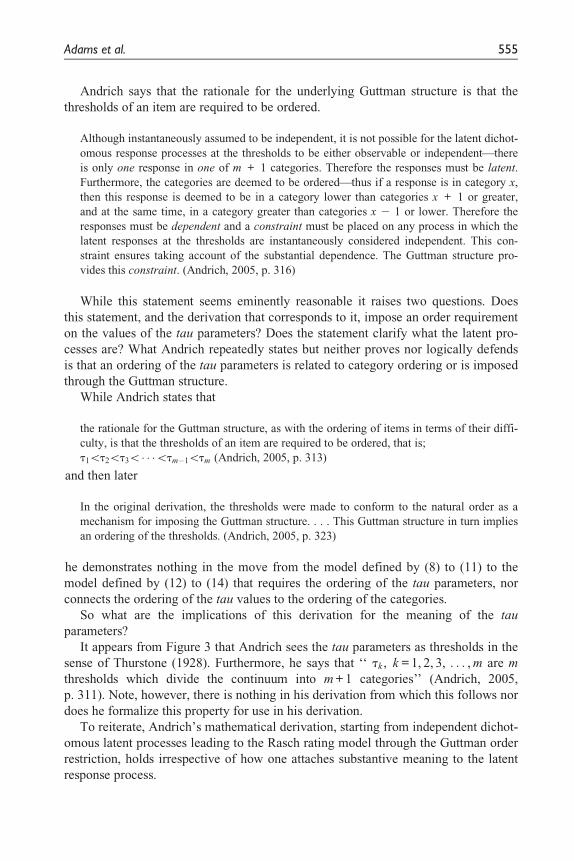
Andrich says that the rationale for the underlying Guttman structure is that the

thresholds of an item are required to be ordered.

Although instantaneously assumed to be independent, it is not possible for the latent dichot-

omous response processes at the thresholds to be either observable or independent—there

is only one response in one of m + 1 categories. Therefore the responses must be latent.

Furthermore, the categories are deemed to be ordered—thus if a response is in category x,

then this response is deemed to be in a category lower than categories x + 1 or greater,

and at the same time, in a category greater than categories x 2 1 or lower. Therefore the

responses must be dependent and a constraint must be placed on any process in which the

latent responses at the thresholds are instantaneously considered independent. This con-

straint ensures taking account of the substantial dependence. The Guttman structure pro-

vides this constraint. (Andrich, 2005, p. 316)

While this statement seems eminently reasonable it raises two questions. Does

this statement, and the derivation that corresponds to it, impose an order requirement

on the values of the tau parameters? Does the statement clarify what the latent pro-

cesses are? What Andrich repeatedly states but neither proves nor logically defends

is that an ordering of the tau parameters is related to category ordering or is imposed

through the Guttman structure.

While Andrich states that

the rationale for the Guttman structure, as with the ordering of items in terms of their diffi-

culty, is that the thresholds of an item are required to be ordered, that is;

t1\t2\t3\� � �\tm�1\tm (Andrich, 2005, p. 313)

and then later

In the original derivation, the thresholds were made to conform to the natural order as a

mechanism for imposing the Guttman structure. . . . This Guttman structure in turn implies

an ordering of the thresholds. (Andrich, 2005, p. 323)

he demonstrates nothing in the move from the model defined by (8) to (11) to the

model defined by (12) to (14) that requires the ordering of the tau parameters, nor

connects the ordering of the tau values to the ordering of the categories.

So what are the implications of this derivation for the meaning of the tau

parameters?

It appears from Figure 3 that Andrich sees the tau parameters as thresholds in the

sense of Thurstone (1928). Furthermore, he says that ‘‘ tk , k = 1, 2, 3, . . . , m are m

thresholds which divide the continuum into m + 1 categories’’ (Andrich, 2005,

p. 311). Note, however, there is nothing in his derivation from which this follows nor

does he formalize this property for use in his derivation.

To reiterate, Andrich’s mathematical derivation, starting from independent dichot-

omous latent processes leading to the Rasch rating model through the Guttman order

restriction, holds irrespective of how one attaches substantive meaning to the latent

response process.

Adams et al. 555

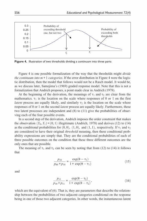
Figure 4 is one possible formalization of the way that the thresholds might divide

the continuum into m + 1 categories. If the error distribution in Figure 4 were the logis-

tic distribution, then the model that follows would not be a Rasch model. It would be,

as we discuss later, Samejima’s (1969) graded response model. Note that this is not a

formalization that Andrich proposes, a point made clear in Andrich (1978).

At the beginning of the derivation, the meanings of t1 and t2 are clear from the

mathematics. t1 is the location on the scale where responses of 0 or 1 on the first

latent process are equally likely, and similarly t2 is the location on the scale where

responses of 0 or 1 on the second latent process are equally likely. Furthermore, these

two latent processes are independent and (8) to (11) give the probabilities of obser-

ving each of the four possible events.

In a second step of the derivation, Andrich imposes the order constraint that makes

the observation Y0, Y1ð Þ = 0, 1ð Þ illegitimate (Andrich, 1978) and derives (12) to (14)

as the conditional probabilities for 0, 0ð Þ, 1, 0ð Þ, and 1, 1ð Þ, respectively. If t1 and t2

are considered to have their original threshold meaning, then these conditional prob-

ability expressions are simply that. They are the conditional probabilities of each of

three possible outcomes on the condition that these three different outcomes are the

only ones that are possible.

The meaning of t1 and t2 can be seen by noting that from (12) to (14) it follows

that

p10

p00 + p10

=exp u� t1ð Þ

1 + exp u� t1ð Þ ð15Þ

and

p11

p10 + p11

=exp u� t2ð Þ

1 + exp u� t2ð Þ , ð16Þ

which are the equivalent of (6). That is, they are parameters that describe the relation-

ship between the probabilities of two adjacent categories conditional on the response

being in one of those two adjacent categories. In other words, the instantaneous latent

00.050.10.150.20.250.3

τ0 τ1

Probability ofexceeding thresholdone, but not two

Probability ofexceeding boththresholds

Figure 4. Illustration of two thresholds dividing a continuum into three parts


events, the probabilities of which are given in (7), are the events of being in the upper

category given that the response is in one of two adjacent categories. The latent pro-

cesses are not therefore those illustrated in Figure 3, which as we have pointed out

would lead to the graded response model, not the Rasch model.

An equivalent, but informative interpretation can be illustrated if (12) to (14) are

laid out in a contingency table as in Table 1.

From this contingency table we immediately see that under the Rasch rating

model:

Pr Y1 = 1ð Þ= exp u� t1ð Þ+ exp 2u� t1 � t2ð Þ1 + exp u� t1ð Þ + exp 2u� t1 � t2ð Þ , ð17Þ

Pr Y2 = 1ð Þ= exp 2u� t1 � t2ð Þ1 + exp u� t1ð Þ + exp 2u� t1 � t2ð Þ , ð18Þ

Pr Y1 = 1jY2 = 0ð Þ= exp u� t1ð Þ1 + exp u� t1ð Þ

=p10

p00 + p10

,

ð19Þ

and

Pr Y2 = 1jY1 = 1ð Þ= exp u� t2ð Þ1 + exp u� t2ð Þ

=p11

p10 + p11

:

ð20Þ

As shown by (17) and (18), the imposed dependence has resulted in both t1 and t2

being involved in describing the difficulties of both of the, now evidently dependent,

latent processes. Furthermore, both t1 and t2 are involved in describing the difficul-

ties of each of the three possible outcomes. The consequence is that the thresholds

should not be interpreted as category difficulties as Andrich attempted to do in Figure

3. Furthermore, if the tau parameters are interpreted as thresholds of an underlying

process, then that process is associated with the conditional probabilities as given in

(19) and (20).

Table 1. The Three Probabilities in Andrich’s Derivation

Pr Y1 = 0ð Þ Pr Y1 = 1ð Þ

Pr Y2 = 0ð Þ p00 = 11 + exp u�t1ð Þ+ exp 2u�t1�t2ð Þ p10 =

exp u�t1ð Þ1 + exp u�t1ð Þ+ exp 2u�t1�t2ð Þ

Pr Y2 = 1ð Þ p01 = 0 p11 =exp 2u�t1�t2ð Þ

1 + exp u�t1ð Þ+ exp 2u�t1�t2ð Þ

Adams et al. 557

In summary, we see two misinterpretations in the language and argument that

Andrich uses when deriving the Rasch rating model. First, the Guttman requirement

does not impose an order requirement on the values of the tau parameters. That is,

the order requirement, that Y0, Y1ð Þ= 0, 1ð Þ is illegitimate, is not a requirement that

t2 must be greater than t1, it just makes certain pairs of events illegitimate. Second,

t1 and t2 cannot be interpreted as the difficulties of thresholds that divide up the

continuum where each person is located.

These misunderstandings about the tau parameters also underpin the oft put argu-

ment that it is illogical to have disordered tau parameters. That is, it is often sug-

gested that there is a problem if the intersection point of scores one and two is at a

lower point on the scale than the intersection point of scores zero and one.

Generically, the argument is put as follows: Suppose we have a three-category

item the scoring of which is as follows: ‘‘0’’ = fail, ‘‘1’’ = pass, and ‘‘2’’ = distinc-

tion. If data are observed for such an item and the estimated parameters are disor-

dered, then the point on the continuum at which a student has an equal probability of

a pass and distinction is at a lower level than the point on the continuum at which a

student has an equal probability of being a fail or a pass. This is seen as illogical.

How can it be that the point at which you are ‘‘tossing up’’ whether a student is a

pass or a distinction is lower than the point at which you are ‘‘tossing up’’ whether a

student is a fail or a pass?

Indeed this does sound odd, but in fact it is a misrepresentation of the situation and

in particular misrepresents the meaning of the conditional probabilities involved. At

the point of equal probability for pass and distinction we are not tossing up if a stu-

dent should be a pass or distinction: In fact we are more confident that they are a fail

(see Figure 5). Similarly at the higher level where fail and pass are equally likely, we

are not tossing up if they should be assigned fail or pass, we are more confident that

they are a distinction.

Definitions of Order

Having questioned the connection between the ordering of the Andrich tau para-

meters and the ordering of the categories, it seems prudent to consider some possible

formal definitions of order.

Order Definition 1

One possible definition of order is the key underpinning of the Masters derivation of

the model. Suppose we consider any two response categories, c1 and c2, of an item.

If c2 is the higher of the two categories, then the probability of a response in category

c2 relative to the probability of a response in category c1 must increase with the latent

variable u: This order requirement can be formalized as follows.

Definition 1. The response categories, c1, c2, . . . , cm, of an item response model

will be considered ordered if


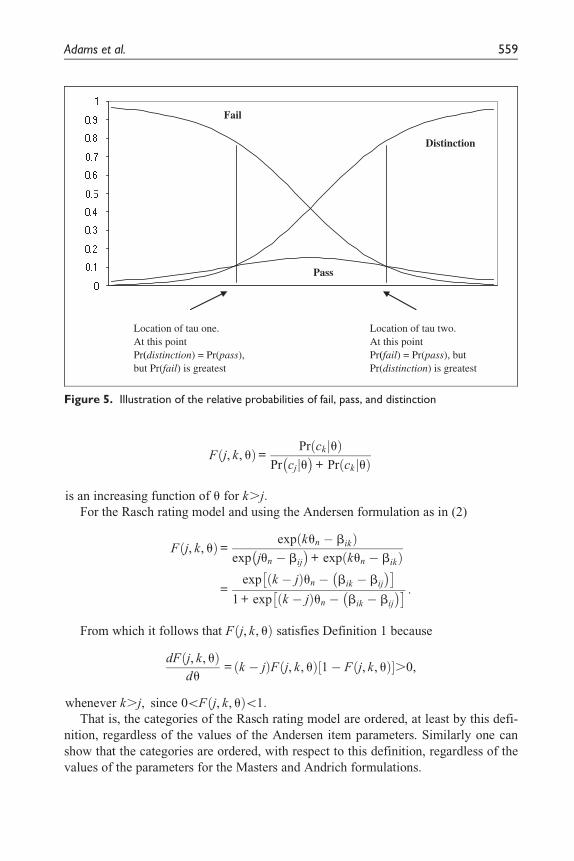
F j, k, uð Þ= Pr ck juð ÞPr cjju� �

+ Pr ck juð Þ

is an increasing function of u for k.j:For the Rasch rating model and using the Andersen formulation as in (2)

F j, k, uð Þ= exp kun � bikð Þexp jun � bij

� �+ exp kun � bikð Þ

=exp k � jð Þun � bik � bij

� �� 1 + exp k � jð Þun � bik � bij

� �� :From which it follows that F j, k, uð Þ satisfies Definition 1 because

dF j, k, uð Þdu

= k � jð ÞF j, k, uð Þ 1� F j, k, uð Þ½ �.0,

whenever k.j, since 0\F j, k, uð Þ\1:That is, the categories of the Rasch rating model are ordered, at least by this defi-

nition, regardless of the values of the Andersen item parameters. Similarly one can

show that the categories are ordered, with respect to this definition, regardless of the

values of the parameters for the Masters and Andrich formulations.

Pass�

��

��

��

��

��

��

��

��

��

�Fail

Distinction

Location of tau one.At this pointPr(distinction) = Pr(pass),but Pr(fail) is greatest

Location of tau two.At this pointPr(fail) = Pr(pass), butPr(distinction) is greatest

Figure 5. Illustration of the relative probabilities of fail, pass, and distinction

Adams et al. 559

Order Definition 2

A second possible definition is one that requires that the expected score on an item be

an increasing function of u. In simple terms, if one respondent has a higher value of u

than another respondent, then, on average, the respondent with the higher u will score

more.

Definition 2. Suppose the scoring function for the categories of item i are given by

jck= k, then the response categories, c1, c2, . . . , cm of an item response model will

be considered ordered if E Xnijuð Þ is an increasing function of u.

For the Rasch rating model and using the Andersen formulation as in (2)

E Xnijuð Þ=Xm

k = 0

kP Xni = kð Þ:

From which it follows that E Xnijuð Þ satisfies Definition 2 because

dE Xnijuð Þdu

=Xm

k = 0

k2P Xni = kð Þ �Xm

k = 0

kP Xni = kð Þ" #2

= var Xnijuð Þ.0

for all u and regardless of the values of the item parameters.

So, as for Definition 1, the categories of the Rasch rating model are ordered,

according to Definition 2, regardless of the values of the item parameters.

Parameter Estimation for the Rasch Rating Model

In the second section, we argued that in the derivation of the Rasch rating model there

is no necessary connection between the ordering of the tau parameters and ordering

of the categories. Then in the third section we proposed two explicit definitions of

order and showed that according to these definitions the categories of the Rasch rat-

ing model are ordered regardless of the values of the tau parameters. In this section,

we review the estimation of the tau parameters and in doing so note two things. First,

if the estimated parameters are ordered it does not necessarily follow that the cate-

gories are ordered according to the order definitions given in the third. Second, for

any given set of abilities the relative frequency of the number of responses in each

category of an item is the only determinant of whether the estimated parameters are

ordered or not.

Let us consider the use of maximum likelihood estimation applied to a set of

L three-category items and a sample of N students for whom ability values are known.

Using the Andrich formulation, as in (3), we have, for n = 1, . . . , N and i = 1, . . . , L

P Xni = knið Þ= 1

gni

expXkni

t = 0

tit + kni un � dið Þ !

, ð21Þ


where ti0 [ 0: Note that for simplicity of the presentation we ignore the additional

required constraint thatPm

t = 0 tit = 0.

As the person parameters are known we can consider the likelihood for the para-

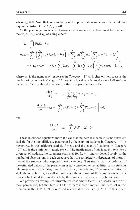
meters, di, ti1, and ti2 of a single item.

Li =YNn = 1

P Xni = knið Þ

log Li =XN

n = 1

Xkni

t = 0

tit + kni un � dið Þ !

�XN

n = 1

logX2

t = 0

expXt

j = 0

tij + j un � dið Þ !

= si1ti1 + si2ti2 � ridi +XN

n = 1

kniun �XN

n = 1

logX2

t = 0

expXt

j = 0

tij + j un � dið Þ !

,

where si1 is the number of responses in Category ‘‘1’’ or higher on item i, si2 is the

number of responses in Category ‘‘2’’ on item i, and ri is the total score of all students

on item i. The likelihood equations for the three parameters are then

∂ log L

∂di

= � ri +XN

n = 1

X2

t = 0

tP Xni = tð Þ= 0,

∂ log L

∂ti1

= si1 �XN

n = 1

P Xni = 1ð Þ+XN

n = 1

P Xni = 2ð Þ" #

= 0,

and

∂ log L

∂ti2

= si2 �XN

n = 1

P Xni = 2ð Þ= 0:

These likelihood equations make it clear that the item raw score ri is the sufficient

statistic for the item difficulty parameter di, the count of students in Category ‘‘1’’ or

higher, si1, is the sufficient statistic for ti1, and the count of students in Category

‘‘2,’’ si2, is the sufficient statistic for ti2. The implication of this is as follows. For a

given set of students, the parameter estimates for di, ti1, and ti2 depend solely on the

number of observations in each category; they are completely independent of the abil-

ities of the students who respond in each category. This means that the ordering of

the estimated values of the parameters is not connected to the abilities of the students

who responded in the categories. In particular, the ordering of the mean abilities for

students in each category will not influence the ordering of the item parameter esti-

mates, which are determined solely by the numbers of students in each category.

We provide an example to illustrate the case where there is a disorder in the esti-

mate parameters, but the item still fits the partial credit model. The item set in this

example is the TIMSS 2003 released mathematics item set (TIMSS, 2003). There

Adams et al. 561

are 99 items in all. The student responses are from the United States data set. A par-

tial credit model is used to fit the item responses. Six of the items are partial credit

items with scores 0, 1, and 2. The remaining items are all dichotomous. All six par-

tial credit items in this data set have disordered thresholds. As an example, we only

show the results for item M032764. The item and the scoring guides are shown in

Figure 6. The item statistics are shown in Figure 7. The item characteristic curves

and the expected scores curve are shown in Figure 8 and Figure 9, respectively.

Figure 6. TIMSS 2003 released mathematics item (M032764)


The item statistics shown in Figure 7 indicate that this item is difficult for the stu-

dents, with 89% of the students obtaining a 0 score. Only 3% obtained a score of 1,

and 8% obtained a score of 2. The item characteristic curves in Figure 8 show a low

curve for score Category 1, reflecting the low frequency of responses for this score

category and resulting in disordered thresholds (3.75 and 0.07).

Despite the disordered thresholds, we first note that the item weighted fit statistic

is 1.00, indicating the item fit the item response model. This is further confirmed by

Figure 8. Item characteristic curves for Item M032764

Cases for this item 1498 Discrimination 0.35Item Threshold(s): 1.83 1.99 Weighted MNSQ 1.00Item Delta(s): 3.75 0.07-------------------------------------------------------------------Label Score Count % of tot Pt Bis Mean Ability------------------------------------------------------------------- 0 0.00 1342 89.59 -0.33 -0.11 1 1.00 42 2.80 0.06 0.67 2 2.00 114 7.61 0.34 1.41===================================================================

Figure 7. Item statistics for Item M032764

Adams et al. 563

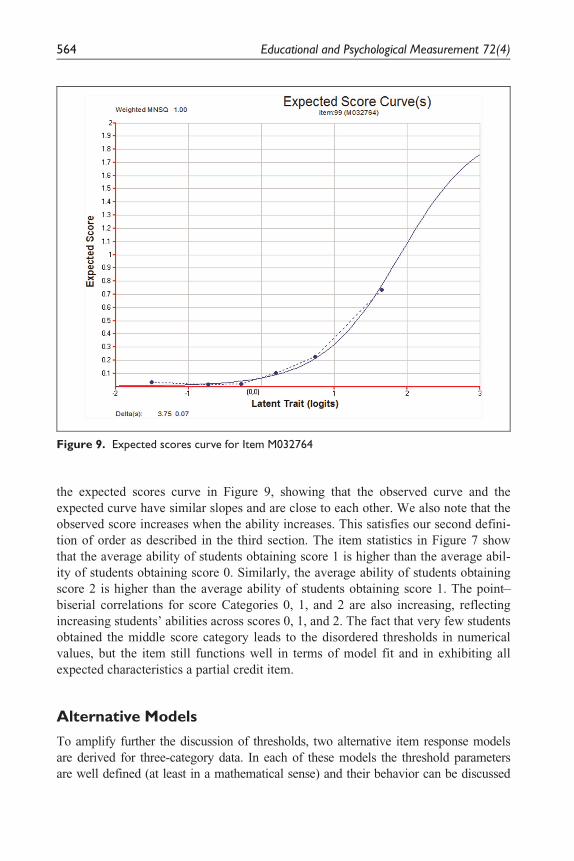
the expected scores curve in Figure 9, showing that the observed curve and the

expected curve have similar slopes and are close to each other. We also note that the

observed score increases when the ability increases. This satisfies our second defini-

tion of order as described in the third section. The item statistics in Figure 7 show

that the average ability of students obtaining score 1 is higher than the average abil-

ity of students obtaining score 0. Similarly, the average ability of students obtaining

score 2 is higher than the average ability of students obtaining score 1. The point–

biserial correlations for score Categories 0, 1, and 2 are also increasing, reflecting

increasing students’ abilities across scores 0, 1, and 2. The fact that very few students

obtained the middle score category leads to the disordered thresholds in numerical

values, but the item still functions well in terms of model fit and in exhibiting all

expected characteristics a partial credit item.

Alternative Models

To amplify further the discussion of thresholds, two alternative item response models

are derived for three-category data. In each of these models the threshold parameters

are well defined (at least in a mathematical sense) and their behavior can be discussed

Figure 9. Expected scores curve for Item M032764


in relation to the parameters of the Rasch rating model. What we shall see at the end of

this section is that even when order of the categories is clearly built into the models, the

equivalent of the Rasch rating model tau parameters will in many cases be disordered.

A Sequential Model

Under the sequential model (Molenaar, 1983) for three response categories we again

hypothesize two latent dichotomous items with response probabilities governed by (7),

but we explicitly make the outcome of the second latent item dependent on the first. In

particular, if the event Y1ð Þ = 0ð Þ occurs, then the probability Pr Y2 = 1ð Þ = 0: Under this

assumption a model for three response categories can be derived as follows:

p00 = Pr Y0, Y1f g = 0, 0f g½ �= Pr Y0f g = 0f g½ � Pr Y1f g = 0f gj Y0f g= 0f g½ �

=1

1 + exp u� t1ð Þ31

=1 + exp u� t2ð Þ

1 + exp u� t1ð Þ½ � 1 + exp u� t2ð Þ½ � ,

ð22Þ


=exp u� t1ð Þ

1 + exp u� t1ð Þ31

1 + exp u� t2ð Þ

=exp u� t1ð Þ

1 + exp u� t1ð Þ½ � 1 + exp u� t2ð Þ½ � ,

ð23Þ


=1

1 + exp u� t1ð Þ30

= 0,

ð24Þ


=exp u� t1ð Þ

1 + exp u� t1ð Þ3exp u� t2ð Þ



1 + exp u� t1ð Þ½ � 1 + exp u� t2ð Þ½ � :

ð25Þ

Under this model the parameters t1 and t2 are the thresholds for the two latent

events with an explicit dependency imposed between the two latent responses. For a

Adams et al. 565

complete discussion of this model, see Verhelst, Glas, and De Vries (1997). Note that

while this model uses the simple logistic model at the level of the latent process, the

combined model for the single three-category item is not a Rasch model in the sense

of Fischer (1995).

A Cumulative Logit Model (Graded Response Model)

Under the cumulative logit model (Agresti, 1990) for three response categories, a

single response mechanism is assumed, but this response process has two thresholds,

t1 and t2: A latent response above t2 yields a ‘‘2’’ response, a latent response

between t1 and t2 yields a ‘‘1’’ response, and a latent response below t1 yields a

‘‘0’’ response. This response process is illustrated in Figure 10. The distribution

shown in Figure 10 is the logistic distribution.

This model is the same model as the graded response model of Samejima (1969)

and is the model that is most commonly used as the measurement model in structural

equation models that permit ordinal responses to items; for example, it is standard in

MPlus (Muthen & Muthen, 2006).

Under this model the probabilities for three response categories are as follows:

p0 =1

1 + exp u� t1ð Þ =1 + exp u� t2ð Þ

1 + exp u� t1ð Þ½ � 1 + exp u� t2ð Þ½ � , ð26Þ

p1 =1

1 + exp u� t2ð Þ �1


=exp u� t1ð Þ � exp u� t2ð Þ


p2 =exp u� t2ð Þ


=exp u� t2ð Þ+ exp 2u� t1 � t2ð Þ1 + exp u� t1ð Þ½ � 1 + exp u� t2ð Þ½ � ,

ð28Þ

00.050.10.150.20.250.3

τ1 τ2

Probability ofscoring one

Probability ofscoring two

Probability ofscoring zero

Figure 10. Illustration of a cumulative logit model


and the parameters t1 and t2 are explicitly defined as the boundaries between the

response categories. In the general case there would be m thresholds that would

divide the continuum into m + 1 categories. Note that the construction of the prob-

abilities is such that t1 and t2 can never be disordered. If they were, expression (27)

would result in a negative probability.

Ordered Partition

We have already introduced the ordered partition model of Wilson (1992); it was

given by (8) to (11). This model is applicable when there are multiple categories of

response but the same score is applied to two or more of the categories. In the form

given by (8) to (11), t1 and t2 are the difficulties of two independent items—for

which, of course, there is no order requirement or expectation.

Graphical Display for the Four Models

In Figure 11, the response probabilities of each of the outcomes for each of the four

models we have discussed so far are plotted for the case where

t1 = � 0:5 and t2 = 0:5 (i.e., the taus are ordered). Recall that under the sequential

model these two parameters describe the difficulty of the first and second items,

respectively, and an attempt at the second item is not permitted if the first item is

failed. Clearly, in each of these cases the categories are ordered.

For the sequential model and the ordered partition model the two parameters are

the difficulties of the two items. For the cumulative model the two parameters are

Sequential Model

0

0.2

0.4

0.6

0.8

1

-4 -3 -2 -1 0 1 2 3 4

Cumulative Logit

0

0.2

0.4

0.6

0.8

1

-4 -3 -2 -1 0 1 2 3 4

Ordered Partition

0

0.2

0.4

0.6

0.8

1

-4 -3 -2 -1 0 1 2 3 4

Rasch Rating Model

0

0.2

0.4

0.6

0.8

1

-4 -3 -2 -1 0 1 2 3 4

0

1

2

0

1

2

0

1

2(0,0)

(1,0)

(1,1)

(0,1)

Figure 11. Response probabilities for the four models

Adams et al. 567

cut points on an underlying continuum. For the Rasch rating model the parameters

describe the intersection points of ‘‘0’’ and ‘‘1’’ and ‘‘1’’ and ‘‘2,’’ respectively.

Each of the graphs in Figure 11 was constructed with the same ordered pair of

parameters. Note, however, that the cumulative logit model, even with ordered

thresholds on the underlying continuum, results in a ‘‘1’’ category that is never most

probable, and the intersection point of ‘‘1’’ and ‘‘2’’ is below the intersection point

of ‘‘0’’ and ‘‘1.’’ If this data pattern were modeled with the Rasch rating model, then

parameter estimates would be disordered and the ordering of the categories would be

refuted. That is, under the cumulative model where the categories are ordered by

construction, it is possible for the intersection point of ‘‘1’’ and ‘‘2’’ to be below the

intersection point of ‘‘0’’ and ‘‘1.’’

In fact, under the cumulative model the intersection points will be reversed when-

ever the difference between the thresholds (the actual category boundaries) is less

than approximately 1.4 logits.

The sequential model too will produce a pattern of reversed intersection points

whenever the difference between the item difficulties is less than about 0.6 logits. So

that even if the tau parameters are ordered and the Guttman process is required (i.e.,

Y0, Y1ð Þ= 0, 1ð Þ is illegitimate), reversed intersection points can occur under the

sequential model.

Modeling Sets of Items With the Rasch Rating Model

A number of authors (Hunyh, 1994, 1996; Verhelst & Verstralen, 1997) have

explored the application of the Rasch rating model to sum scores for sets of items

that conform to the simple logistic model. Their work has shown that if individual

items conform to the simple logistic model, then a Rasch rating model will hold for

the sum scores. Furthermore, under these circumstances the threshold parameters for

the Rasch rating model must be ordered. The interesting consequence of this is that

if a Rasch rating model is applied to a set of sum scores and the parameter estimates

are not ordered, then the individual items cannot be modeled with a simple logistic

model that assumes item (local) independence. Verhelst and Verstralen (1997), in

particular, show that when modeling sum scores the Rasch rating model permits a

wide variety of dependencies among the underlying items. Furthermore, exploration

of this issue would seem to be a fruitful path to follow in terms of testing for item

dependency with the Rasch model.

Here, we illustrate the findings of the work of Hunyh and Verhelst and Verstralen

for the very simple case of two dichotomous items.

If we have two independent items, Y1 and Y2, that conform to the simple logistic

model with item difficulty parameters a1 and a2, then the probabilities of the sum

scores are as follows:

Pr Y1 + Y2 = 0ð Þ= 1

1 + exp u� a1ð Þ½ � 1 + exp u� a2ð Þ½ � , ð29Þ


Pr Y1 + Y2 = 1ð Þ= exp u� a1ð Þ+ exp u� a2ð Þ1 + exp u� a1ð Þ½ � 1 + exp u� a2ð Þ½ � , ð30Þ

and

Pr Y1 + Y2 = 2ð Þ= exp 2u� a1 � a2ð Þ1 + exp u� a1ð Þ½ � 1 + exp u� a2ð Þ½ � : ð31Þ

Applying the Rasch rating model to the sum scores, the probabilities of the sum

scores are, using the Masters parameterization, as follows:

Pr Y1 + Y2 = 0ð Þ = 1

1 + exp u� d1ð Þ + exp 2u� d1 � d2ð Þ , ð32Þ

Pr Y1 + Y2 = 1ð Þ = exp u� d1ð Þ1 + exp u� d1ð Þ + exp 2u� d1 � d2ð Þ , ð33Þ

and

Pr Y1 + Y2 = 2ð Þ= exp 2u� d1 � d2ð Þ1 + exp u� d1ð Þ+ exp 2u� d1 � d2ð Þ : ð34Þ

The Rasch rating model ((32) to (34)) is equivalent to the simple logistic model

((29) to (31)) since the following functional relationships between the parameters can

be established:

e�a1 = e�d1 + e�d2 and e�a2 =e�d1 e�d2

e�d1 + e�d2ð35Þ

e�d1 = e�a1 + e�a1 and e�d2 =e�a1 e�a1

e�a1 + e�a1: ð36Þ

Having established this relationship, it is also possible to show that if the Rasch

rating model is applied to sum scores on items that conform to the simple logistic

model, then the parameters of the Rasch rating model must be ordered. In this simple

case a proof using reductio ad-absurdum is as follows.

If d1.d2, then

� d1\� d2

) exp �d1ð Þ\exp �d2ð Þ

) exp �a1ð Þ+ exp �a2ð Þ\ exp �a1ð Þ exp �a2ð Þexp �a1ð Þ+ exp �a2ð Þ

) exp �a1ð Þ+ exp �a2ð Þð Þ2\exp �a1ð Þ exp �a2ð Þ) exp �2a1ð Þ+ 2 exp �a1ð Þ exp �a2ð Þ+ exp �2a2ð Þ\exp �a1ð Þ exp �a2ð Þ) exp �2a1ð Þ+ exp �a1ð Þ exp �a2ð Þ+ exp �2a2ð Þ\0,

Adams et al. 569

which cannot be true, so we conclude that if the two sets of equations (29) to (31)

and (32) to (34) are equivalent for all values of theta, then it must be the case that

d1 � d2:

Discussion

We have argued that the ordering of the Rasch rating model thresholds is not con-

nected to the ordering of the item response categories and that they cannot be inter-

preted as thresholds on an underlying continuum. In making this observation we do

not dismiss the possibility that disordered estimated parameters may well be an indi-

cator of a problem with an item. First, our discussion above, for example, has shown

that if the Rasch rating model is applied to sum scores, then estimated parameter dis-

order is an indicator of dependence among the underlying items. Second, Andrich has

shown that variations in the discrimination between adjacent categories can result in

disordered estimated parameters. Third, disordered parameter estimates are indicative

of low frequencies in a response category. There are a number of reasons why this

may be an issue of concern, and whenever it occurs, it should be carefully reviewed

by scale constructors.

While we have shown that the Andrich derivation does not depend on the nature

of the latent processes and fails to demonstrate that the Guttman requirement for the

latent processes imposes a numerical ordering on the tau parameters, we do not dis-

miss the observation that if certain psychological processes are assumed, then a

numerical ordering of the tau parameters would be a substantive requirement.

If we accept the scenario of judges making independent dichotomous judgments,

as illustrated in Figure 3, and then bringing them together and only accepting pat-

terns that confirm to the Guttman requirement, then the tau parameters are estimates

of the thresholds displayed in Figure 3 and disorder is a concern. The problems are,

however, that we do not know the process that judges have used to produce their rat-

ings, the model’s derivation is silent on the nature of the process, and the meaning of

the parameters as thresholds requires unverifiable assumptions concerning the nature

of the latent processes. The only thing that can be verified is that the tau parameters

describe the events given by (15) and (16), the events of being in the upper category

given that the response is in one of two adjacent categories.

What we are concerned about, however, is proliferation of the view that disordered

parameters are indicative of a set of items that are not working because the categories

are not ordered. As we have argued above, this is not the case; parameter disorder

does not imply category disorder, unless a particular latent process is assumed; a pro-

cess that can only hold when judges are involved in some judgment processes and

even then the process is merely conjecture.

In perhaps the majority of applications of the Rasch rating model, no judges are

involved. For example, an item may have four possible (exact) answers that are

deemed appropriate to be scored as ‘‘0,’’ ‘‘1,’’ ‘‘2,’’ and ‘‘3,’’ respectively. In this

case, the stochastic nature of the response resides with the student, and not with any


judges, as the judgments are completely objective (because the possible answers are

unambiguous). It is difficult to conceive this situation in terms of students making

decisions between adjacent categories when responding. A student may provide an

answer without even being aware what other possible answers there may be. In this

case, under the model, students with a particular ability will have certain probabil-

ities of providing particular answers.

The occasionally observed practice of categories being recoded to change the

order on the basis of disordered parameter estimates is of particular concern as is the

practice of routinely collapsing categories if the parameter estimates are not ordered

(Zhu 2002; Zhu, Updyke, & Lewandowski, 2001). All these practices, when carried

out solely on the basis of disordered thresholds, should be avoided.

Furthermore, we also note that the review of parameter disorder often takes place

without due consideration being given to the standard errors of the parameter esti-

mates and the covariance between them. If parameter order is of interest, then an

appropriate asymptotic test of disorder, for a pair of threshold estimates, would take

the form

d =t2 � t1ffiffiffiffiffiffiffiffiffiffiffiffiffiffiffiffiffiffiffiffiffiffiffiffiffiffiffiffiffiffiffiffiffiffiffiffiffiffiffiffiffiffiffiffiffiffiffiffiffiffiffiffiffiffiffiffiffiffiffiffi

var t1ð Þ+ var t2ð Þ+ 2cov t1, t2ð Þp , ð37Þ

where d was asymptotically distributed as a standard normal deviate. Adams (1989)

has shown that the covariance term in (37) can be quite large relative to the other

terms in the denominator and should not be ignored.

As a final point we acknowledge that it is important to recognize that disordered

parameter estimates may well be an indicator of an item that is not functioning as

intended. It may, for example, indicate that some middle categories are not useful

because very few respondents are using them. Furthermore, it may well indicate

issues with the discrimination of the item; recall that the Rasch rating model requires

equal discrimination for each of the latent processes. Items with disordered para-

meter estimates need to be reviewed with regard to these issues.

Declaration of Conflicting Interests

The author(s) declared no potential conflicts of interest with respect to the research, authorship,

and/or publication of this article.

Funding

The author(s) received no financial support for the research, authorship, and/or publication of

this article.

Note

1. Actually we are following the notation of Andrich (2005, Equation 5), which uses integer

scoring functions and allows the threshold parameters, tik , to vary across items.

Adams et al. 571

References

Adams, R. J. (1989). Estimating measurement error (Unpublished doctoral dissertation).

University of Chicago.

Agresti, A. (1990). Categorical data analysis. New York, NY: John Wiley.

Andersen, E. B. (1973). Conditional inference for multiple choice questionnaires. British

Journal of Mathematical and Statistical Psychology, 26, 31-44.

Andersen, E. B. (1977). Sufficient statistics and latent trait models. Psychometrika, 42, 69-78.

Andrich, D. (1978). A rating formulation for ordered response categories. Psychometrika, 43,

561-573.

Andrich, D. (2005). The Rasch model explained. In S. Alagumalai, D. D. Durtis, & N. Hungi

(Eds.), Applied Rasch measurement: A book of exemplars (pp. 308-328). Berlin, Germany:

Springer-Kluwer.

Andrich, D., Sheridan, B., & Luo, G. (2003). RUMM2020: A Windows program for the Rasch

unidimensional measurement model. Perth, Australia: RUMM Laboratory.

Fischer, G. H. (1995). The derivation of polytomous Rasch models. In G. H. Fischer & I. W.

Molenaar (Eds.), Rasch models: Foundations, recent developments and applications (pp.

292-305). New York, NY: Springer Verlag.

Hunyh, H. (1994). On equivalence between a partial credit items and a set of independent

Rasch binary items. Psychometrika, 59, 111-119.

Hunyh, H. (1996). Decomposition of Rasch partial credit item into independent binary and

indecomposable trinary items. Psychometrika, 61, 31-39.

Linacre, J. M. (1991). Step disordering and Thurstone thresholds. Rasch Measurement

Transactions, 5, 171.

Masters, G. N. (1980). A Rasch model for rating scales (Unpublished doctoral dissertation).

University of Chicago.

Masters, G. N. (1982). A Rasch model for partial credit scoring. Psychometrika, 47, 149-174.

Molenaar, I. W. (1983). Item steps (Heymans Bulletin HB-83-630-EX). Groningen, Germany:

University of Groningen.

Muthen, L. K., & Muthen, B. O. (2006). Mplus user’s guide [Computer software and manual]

(4th ed.). Los Angeles, CA: Muthen & Muthen.

Nijsten, T., Sampogna, F., Chren, M., & Abeni, D. (2006). Testing and reducing Skindex-29

using Rasch analysis: Skindex-17. Journal of Investigative Dermatology, 126, 1244-1250.

Nilsson, A. L., Sunnerhagen, K. S., & Grimby, G. (2007). Scoring alternatives for FIM in

neurological disorders applying Rasch analysis. Acta Neurologica Scandinavica, 111, 264-

273.

Rasch, G. (1961). On general laws and the meaning of measurement models in psychology. In

Proceedings of the IV Berkeley Symposium on Mathematical Statistics and Probability (pp.

321-333). Berkeley: University of California Press.

Samejima, F. (1969). Estimation of latent ability using a response pattern of graded scores.

Psychometrika Monographs, 34(Suppl. 17), 386-415.

Thurstone, L. L. (1928). Attitudes can be measured. American Journal of Sociology, 33, 529-

554.

TIMSS. (2003). TIMSS 2003 Released items. Retrieved from http://timss.bc.edu/timss2003i/

released.html

Verhelst, N. D., Glas, C. A. W., & De Vries, H. H. (1997). A steps model to analyze partial

credit. In W. J. Van der Linden & R. K. Hambleton (Eds.), Handbook of modern item

response theory (pp. 123-138). New York, NY: Springer-Verlag.


Verhelst, N. D., & Verstralen, H. H. F. M. (1997). Modeling sums of binary items by the partial

credit model (Measurement and Research Department Research Report 97-7). Arnhem,

Netherlands: Cito.

Wilson, M. (1992). The ordered partition model: An extension of the partial credit model.

Applied Psychological Measurement, 16, 309-325.

Wilson, M. R., & Adams, R. J. (1993). Marginal maximum likelihood estimation for the

ordered partition model. Journal of Educational Statistics, 18, 69-90.

Wilson, M. R., & Adams, R. J. (1995). Rasch models for item bundles. Psychometrika, 60,

181-198.

Wu, M. L., Adams, R. J., & Wilson, M. R. (1997). ConQuest: Multi-Aspect Test Software

[Computer program]. Camberwell, Australia: Australian Council for Educational Research.

Zhu, W. (2002). A confirmatory study of Rasch-based optimal categorization of a rating scale.

Journal of Applied Measurement, 3, 1-15.

Zhu, W., Timm, G., & Ainsworth, B. A. (2001). Rasch calibration and optimal categorization

of an instrument measuring women’s exercise perseverance and barriers. Research

Quarterly for Exercise and Sport, 72, 104-116.

Zhu, W., Updyke, W. F., & Lewandowski, C. (1997). Post-hoc Rasch analysis of optimal

categorization of an ordered-response scale. Journal of Outcome Measurement, 1, 286-304.

Adams et al. 573

the rasch rating model and -...

Documents