the recipe for high health spending - lund...
TRANSCRIPT

Lund University WPMM 40
Department of Political Science Tutor: Moira Nelson
The Recipe for
High Health Spending:
A Qualitative Comparative Analysis of Indonesian Districts
Erric Fadhli

Acknowledgements
First, I would like to thank to Allah SWT who always gives me strength and
guidance. Second, I want to give my sincere thanks for all my family back home
in Indonesia, especially for both of my parents in two cities who always saying
my name in their prayers days and nights. Third, I would like to give my biggest
thank to my wife Dhina Fibrianti who always beside me and give me her hands
when I was facing some hardest time in writing this thesis. Fourth, I would like to
thank to my supervisor Moira Nelson for always giving me advices and great
support for my thesis. To my knowledge, she is the most dedicated teacher in
Political Science Department Lund University. Therefore, I was very lucky to
have her as my supervisor. I pray for her more successful career in the future.
Fifth, I would like to give my gratitude to my examiner Ylva Stubbergaard for her
constructive critiques and comments. Those are really useful for my work now
and in the future. Lastly, I thank to all Indonesian students in Lund whom I cheer
together in facing the cold and dark Northern European winter and for Antony Lee
for giving his precious time in preparing the final presentation. Thanks bro!

Abstract
This study investigates the path to high health spending among local governments
in Indonesia under the setting where administrative, fiscal, and political
decentralization are already in place. The motivation behind this study is that
Indonesia still has low level of health outcomes. Small amount of health spending
is one prominent reason for this lack of achievement. However, the effort in
improving health outcomes and its spending today in Indonesia is not solely in the
hand of central government. After decentralization, local governments play a
decisive part in executing the health policy. In practice, the level of health
spending among local governments in Indonesia is contrast. Therefore, conducting
comparison is one promising strategy to observe this phenomenon. By utilizing
fsQCA, this study compares several conditions in one model that seems likely to
improve health spending among 295 local governments in Indonesia. This study
proposes, local direct election, high central transfer, good leadership, and high
social pressure is the combination that likely leads to high local health spending.
Based on the evidence presented in this study, the combination of high central
transfer and high social pressure is the path to the high health spending.
Keywords: Decentralization, Direct Election, Health Spending, Indonesia, fsQCA.
Words: 18.676

Contents
1. Introduction ............................................. ........................................................ 1
1.1 Health Condition in Indonesia .................................................................. 1
1.2 Research Problem and Question .............................................................. 3
1.3 Outline ...................................................................................................... 4
2. The Background: Decentralization ................................................................ 6
2.1 Concept of Decentralization ..................................................................... 6
2.1.1 Decentralization ............................................................................ 6
2.1.2 Forms of Decentralization ............................................................ 6
2.1.3 Dimensions of Decentralization ................................................... 8
2.2 Decentralization in Indonesia ................................................................... 9
2.2.1 New Order Era .............................................................................. 9
2.2.2 “Big Bang” ................................................................................... 10
2.2.3 Post New Order ............................................................................ 12
3. Determinants of Health Spending .................................................................. 14
3.1 Local Direct Election ............................................................................... 14
3.1.1 Theory of Electoral Institutions .................................................... 14
3.1.2 Literature Review on Local Direct Election ................................. 16
3.2 Central Transfer ........................................................................................ 18
3.2.1 Concept of Intergovernmental Transfers ...................................... 18
3.2.2 Literature Review on Central Transfer ......................................... 18
3.3 Leadership ................................................................................................ 20
3.3.1 Theory of Transformational Leadership ....................................... 20
3.3.2 Literature Review on Local Leadership ....................................... 21
3.4 Social Pressure ......................................................................................... 22
3.4.1 Theory of Public Control .............................................................. 22
3.4.2 Literature Review on Social Pressure ........................................... 23
3.5 Where this study goes from here? ............................................................ 24
4. Methodology ..................................................................................................... 26
4.1 A Configurational Comparative Method .................................................. 26
4.2 Qualitative Comparative Analysis (QCA) ............................................... 27

4.2.1 Case Selection .............................................................................. 29
4.2.2 Variables ....................................................................................... 30
4.2.2.1 Outcome ......................................................................... 31
4.2.2.2 Conditions ...................................................................... 32
4.2.3 Data ............................................................................................... 34
5. Analysis ............................................................................................................. 37
5.1 Calibration Procedure ............................................................................... 37
5.2 Necessity Conditions ................................................................................ 43
5.3 Truth Table Analysis ................................................................................ 46
6. Result and Interpretation ................................................................................ 52
6.1 Result ........................................................................................................ 52
6.2 Interpretation ............................................................................................ 54
7. Conclusion ........................................................................................................ 57
7.1 Limitation and Future Studies .................................................................. 57
8. References ......................................................................................................... 58
Appendix 1.1
Appendix 1.2

List of Abbreviations
ASEAN Association of Southeast Asian Nations
BPS Badan Pusat Statistik/Statistics Indonesia
CETRO Center for Electoral Reform
csQCA Crisp Set Qualitative Comparative Analysis
DAK Dana Alokasi Khusus/Specific Allocation Grant
DAU Dana Alokasi Umum/General Allocation Grant
DPRDs Local Representatives
fsQCA Fuzzy Set Qualitative Comparative Analysis
GDP Growth Domestic Product
IDR Indonesian Rupiah
INDO-DAPOER Indonesia Database for Policy and Economic Research
KPPOD Regional Autonomy Watch
KPUDs Regional Election Commissions
MK Mahkamah Konstitusi/Constitutional Court
MMR Maternal Mortality Rate
MoF Ministry of Finance
MoHA Ministry of Home Affairs
NDI National Democratic Institute
NGOs Non-governmental Organizations
UHC Universal Health Coverage
U5MR Under-five Mortality Rate
QCA Qualitative Comparative Analysis
WDI World Development Indicators
WHO World Health Organization

List of Graph, Tables, and Appendixes
Graph
Graph 1.1 Trend of Central Government Spending Based on Functions, 2005–
2011
Tables
Table 1.1 Health Outcomes among ASEAN Developing Countries in 2011
Table 4.1 Descriptive Statistics
Table 5.1 Local Direct Election in Indonesia, 2005 – 2011
Table 5.2 Four-value Fuzzy Set
Table 5.3 Direct Calibration Thresholds
Table 5.4 Set Relation of Outcome as the Subset of Conditions (Necessity)
Table 5.5 Example of Fuzzy Operations
Table 5.6 Truth Table Analysis
Table 5.7 Truth Table Consistency Thresholds
Table 6.1 Solutions
Appendixes
Appendix 1.1 Raw Dataset
Appendix 1.2 Fuzzy Sets Scores

1
1 Introduction
1.1 Health Condition in Indonesia
Health is an essential sector in Indonesia. For example, health is among sectors
that have an explicit purpose to pursue Millennium Development Goals (MDGs)
by 2015.1 Moreover, Indonesia is also aiming to achieve universal health coverage
(UHC) for all Indonesian by 2019 (Harimurti et al. 2013 p v). However, despite
its importance, Indonesia still relatively has low level of health funding.
In Indonesia, the combination between public-private provisions funds health
services. However, the leading role and the majority source of funding are still in
the hand of the public sector (Ibid p 5).
Graph 1.1: Trend of Central Government Spending Based on Functions,
2005 - 2011 (In Million IDR)
Source: Author’s compilation based on the data from the Ministry of Finance (MoF).
Notes: 2005 & 2006 are realization and 2007 – 2011 are allocation data.
As displayed by Graph 1.1, the trend of government health spending in
Indonesia has slightly improved after 2005. However, from 2007 to 2009, it
1 Health sector is intended to pursue specifically goals number four, five, and six (UN 2015). The information is
available here: http://www.un.org/millenniumgoals/
IDR 0
IDR 20.000
IDR 40.000
IDR 60.000
IDR 80.000
IDR 100.000
IDR 120.000
2005 2006 2007 2008 2009 2010 2011
Education
Economy
Housing
Security
Health

2
leveled out and then decreased in 2010. Moreover, the comparison between health
spending and several development sectors’ expenditures also portrays a rather
contrasting figure. The spending on health compared with these sectors is
substantially small, particularly with education and economy sector.
Consequently, Indonesia has low scores on several health outcomes. In 2011,
Indonesians had a slightly lower level of life expectancy at 70 years compared
with the average of ASEAN developing countries’ score at 71 years. Moreover,
Indonesia also had inferior results in measles vaccination rate and maternal
mortality rate (MMR) compared with its ASEAN neighbors, most notably with
Malaysia and Thailand (see Table 1.1).
Table 1.1: Health Outcomes among ASEAN Developing Countries in 2011
Country
GDP
Per
Capita
(US$)
Total Life
Expectancy
at Birth
(years)
U5MR
(per 1,000
live
births)*
Measles
Rate
(%)
MMR
(per
100,000 live
births)**
Cambodia 810 71 42 93 200
Indonesia 2,920 70 32 80 210
Lao DPR 1,090 67 77 69 270
Malaysia 8,840 75 9 95 31
Myanmar - 65 54 88 220
Philippines 2,620 68 31 79 120
Thailand 4,620 74 14 98 28
Vietnam 1,390 75 25 96 51
Average 3,184*** 71 35 87 141 Source: Author’s compilation based on the data from World Development Indicators (2015).
Notes: * = Under-five Mortality Rate (U5MR) the score is the lower, the better, ** = Maternal
Mortality Rate (MMR) data from 2010 and the score is the lower, the better, and *** = without
Myanmar.
Given these facts, resources become one prominent concern for Indonesia in
order to increase its health outcomes. Accordingly, in order to improve its health
outcomes, first critical requirement for Indonesia is to invest more in its health
sector (Kristiansen & Santoso 2006 p 258; Simatupang 2009 p 89).
However, it is worth to note that the effort in improving health spending in
Indonesia is not solely in the hand of central government. Indonesia has been
practicing decentralization since the end of the twentieth century or right after the
demise of the authoritarian New Order regime in 1999. Decentralization has
devolved the responsibility of public sector to provide public services including

3
health to the local level. Decentralization gives a strong message that the local
governments have become decisive players in improving the health sector
especially after the implementation of fiscal decentralization where the majority
of health budget is transferred to district level (Simatupang 2009 p 20; Harimurti
et al. 2013 p 7). Moreover, the implementation of the local direct election in 2005
has also brought the opportunity to strengthen the execution of fiscal
decentralization. Directly elected local leaders are expected to accelerate the
improvement of health outcomes by spending more in social sectors including
health sector (Skoufias et al. 2011 p 11 & 2014 p 16).
1.2 Research Problem and Question
Examining the data disaggregated by districts, local health spending among
Indonesian districts varies considerably. Some districts, indeed, still have a low
level of health spending (e.g., Lampung Tengah regency only has IDR 9,318 per
capita in 2012).2 However, some of them already have a significant high level of
health spending (e.g., Kaimana regency has IDR 2,061,491 per capita in 2012).3
Looking at these contrasting numbers, these distinctive results leave a question on
why those differences happened among those districts.
Several studies have been conducted to observe the impacts of
decentralization especially through local direct election on local health spending
in Indonesia. However, the results are relatively inconclusive and rather
conflicting. For example, a study by Skoufias et al. (2014) concluded that the
implementation of the local direct election had only a weak impact on domestic
health spending. On the other hand, Kis-Katos & Sjahrir (2014 p 5) concluded
that the local direct election had no effect on local health expenditure.
Therefore, this study argues that several other factors may also play a
prominent role to affect local health spending besides local direct election such as
local financial resources, leadership characteristics, as well as local social
pressure. Furthermore, observing these factors and their combinations in order to
find the similarities and differences within those districts is one favorable strategy
2 This amount is based on the data from the World Bank’s INDO-DAPOER (please see Appendix 1.1). 3 This amount is based on the data from the World Bank’s INDO-DAPOER (please see Appendix 1.1).

4
in order to unravel the paths that lead to high local health spending as well as
provide preliminary answer to solving the problem of health outcomes in
Indonesia.
Equipped with the motivation. Therefore, this study raises the question:
“What are the paths to high health spending among local governments in
Indonesia after the implementation of local direct election?”
One promising approach to answering the research question is by conducting
a configurational comparison. Moreover, one particular technique in a
configurational comparative approach is Qualitative Comparative Analysis
(QCA). This particular method, through examining various factors as well as their
combinations, is capable to reveal the path without ignoring the notion of causal
complexity (Ragin 2008 & 2014; Kenworthy & Hicks 2008; Rihoux & Ragin
2009; Schneider & Wagemann 2012).
Accordingly, the aim of this study is to find the paths that lead to high health
spending among local governments in Indonesia. Moreover, this paper adds to the
stock of growing empirical evidence on the advantages and disadvantages of the
decentralization especially in developing countries under the setting where
administrative, fiscal, and political decentralization are already in place. This
research also complements previous studies on health policy by employing a
relatively new model as well as new approach in investigating the problem of
health sector.
1.3 Outline
The remainder of this study is organized as follows. Chapter 2 is dedicated to
explaining the decentralization concept in general as well as the decentralization
reforms in Indonesia and explains how the decentralization system empowers
local governments to have more power and authority to manage their own
jurisdictions. The decentralization system and reforms in Indonesia are explained
in order to show the background setting of this study. Chapter 3 discusses the
determinants of local health spending where the implementation of the local direct

5
election, the central transfer, the local leadership, and the social pressure are taken
into consideration. Chapter 4 explains the methodology and the data that
employed. In chapter 5, the main analysis of the study is described with utilizing
QCA particular tool namely the truth table. In chapter 6, the findings are
interpreted. Finally, chapter 7 wraps up this study.

6
2 The Background: Decentralization
2.1 Concept of Decentralization
This part explains the concept of decentralization in general as well as clarifies its
various forms and dimensions. This section aims to give the reader some initial
insights on decentralization concept which is useful for reading this study further.
2.1.1 Decentralization
Is not easy to define decentralization in simplest meaning as possible since it
covers many forms and works across dimensions. Nevertheless, this study uses
the relatively comprehensive definition of decentralization by Rondinelli (1981)
since it not only captures the core definition of decentralization but also depicts
decentralization fairly.
According to Rondinelli (1981 p 137), decentralization defined as the transfer
of power and authority in planning, decision-making, implementing, managing
public roles as well as responsibilities for public tasks from the central
government and its representatives to their field agencies and to other various
institutions from lower units of government or semi-autonomous public
companies or autonomous local governments or non-governmental organizations
(NGOs) or voluntary organizations or private sectors.
2.1.2 Forms of Decentralization
Decentralization has various forms. Rondinelli (1981 p 137) differentiates the
form of decentralization into two types. The first is functional and areal
decentralization. The functional decentralization refers to the transfer of authority
to execute the particular task to particular institutions that work at national level or
among local governments, for example, field agencies from central ministries that

7
handling health or education missions. The areal decentralization refers to the
transfer of authority to accomplish public tasks to institutions within well-defined
political boundaries such as regency, city, and province.
The second form involves the three degrees of decentralization namely
deconcentration, delegation, and devolution. Deconcentration refers to the shift of
obligation from central governments to staff located at local representative offices
without authority to perform the jobs freely, in other words central government
commands on how to perform the tasks (Rondinelli 1981 p 137; Rondinelli 1983
p 14-15). Therefore, deconcentration considered as the lowest form of
decentralization, and some argue that this form of decentralization is unlikely to
bring advantages, but only disadvantages of decentralization (Litvack et al. 1998 p
4). Moreover, this kind of decentralization is usually happened in unitary
countries without independent local governments where central field agencies are
only to execute public services delivery in more effective and efficient manner
(Ibid p 4).
The second degree of decentralization is called delegation, it refers to the
transfer of authority and responsibility for policy-making and management of
specific public tasks from central government to local governments or other
institutions that not under direct control of central government, but completely
accountable for those tasks (Ibid p 6). Therefore, this form of decentralization
represents a more extensive form of deconcentration, and it also perceived as a
strategy to remove some functions from inefficient government bureaucracies as
well as the strategy of central government to keep highly profitable resources
(Rondinelli 1983 pp 19-20).
The last form of decentralization is devolution. Devolution refers to the
transfer of authority for decision-making, finance, and management to
autonomous local governments that outside the control of central government
(Litvack et al. 1998 p 6). As Rondinelli (1981 p 138 & 1983 p 25) also stated that
this is the most extreme form of decentralization where local governments should
be given full authority to exercise their public tasks within clear geographical
boundaries and without under direct control from central government.

8
2.1.3 Dimensions of Decentralization
Observing several dimensions of decentralization from political, administrative,
and fiscal dimension is beneficial to the fruitful understanding of decentralization.
Yet, there is sometimes overlap and fuzzy definition in describing any of these
dimensions. Moreover, all these dimensions can transform within dimensions and
even into multi-dimensions at once across governments and sectors. Therefore,
exposing some preliminary boundaries of these dimensions is essential when
observing decentralization in general.
The first dimension is the political dimension of decentralization. This
dimension denotes that the process of selection and competition of local
representatives and local leaders through instrument of election or appointment
lets citizens to choose better their representatives and leaders as well as to make
those elected officials deliver better the needs of their citizens or, in other words,
accountable (Ivanyna & Shah 2012 p 5). An example of this dimension is the
implementation of the election at the local level to elect local representatives and
local leaders by local citizens (Ahmad et al. 2008 p 4).
The second dimension is the administrative dimension of decentralization.
This dimension suggests that the transfer of responsibility for the planning,
financing, executing, and management of some public tasks from the central
government and its agencies to field representatives of government agencies or
local governments or public companies or NGOs or voluntary organizations or
private sectors. This dimension in its practical application involves the three
degrees of decentralization namely deconcentration, delegation, and devolution. In
other words, this dimension denotes the application of power transfer into
regulatory actions (Litvack et al. 1998 p 6; Ivanyna & Shah 2012 p 5).
The third is the fiscal dimension of decentralization. This dimension centers
on the financial arrangement and responsibility as a fundamental element of
decentralization (Ahmad et al. 2008 p 4). This dimension sets the financial
arrangements including collecting local taxes or receiving intergovernmental
transfer as well as the decisions about spending (Litvack et al. 1998 p 6).
Moreover, fiscal decentralization comes in various forms including own revenue
from taxes or charges, intergovernmental transfers, and borrowing (Litvack et al.

9
1998 pp 11–12; Ahmad et al. 2008 p 4). However, in many developing countries,
the major source of fiscal decentralization is intergovernmental transfers. In these
countries, usually local governments still rely heavily on central transfer even
though some of them already had the authority to levy taxes.
In addition, some governments also shift responsibility for functions from the
public to the private sector, the practice that called as privatization. Privatization
lets tasks that had been mainly or exclusively the responsibility of government to
be carried out by private sectors such as businesses enterprises or community
groups or NGOs (Rondinelli et al. 1983 p 28).
2.2 Decentralization in Indonesia
In Indonesia, decentralization reforms happened in staggered manner within three
distinctive phases. It is important to observe the changes that occurred in these
stages through the three dimensions of decentralization since it constructs the
form and the practice of current decentralization in Indonesia.
2.2.1 New Order Era
In New Order era, Indonesia was under a highly centralized and autocratic
government. However, despite practicing a high-centralized form of government,
the central government has started giving some “half-heartedly” decentralization
practice to local governments through Law 5/1974. This law introduces lower
degree practices of decentralization including exclusive election only to the
second tier of local government namely regencies and cities. Moreover, provinces
as the first tier of local government were excluded from the practices because
some experiences with separatism movement that happened in 1950s (Simatupang
2009 p 6). In this era, the Ministry of Home Affairs played a prominent role in
organizing all political selection and appointing local representatives from an
exclusive list of nominees (Skoufias et al. 2011 p 5). Administratively, according
to Law 5/74, local governments in Indonesia consist of a local leaders, executive
field agencies, and local representatives (DPRDs) (Ibid p 5). Fiscally, local

10
governments in Indonesia were highly reliant on central government transfers as
well as had limited own source incomes (Ibid p 5).
Nevertheless, in practice, this law was never fully executed as the regime
under New Order was focused more to enhance political stability and regional
unity in response to the communist revolution in 1965 (Simatupang 2009 p 6).
2.2.2 “Big Bang.”
Asian Financial Crisis in 1997 played a decisive role in the fall of New Order
regime as well as in the implementation of “real” decentralization. Besides, the
central government was also in urgent need to implement decentralization reform
to suppress the growing demands of independence from provinces that had
dissatisfaction with the central government and had long history of armed conflict
such as Aceh (Simatupang 2009 p 6; Kis-Katos & Sjahrir 2014 p 6). Therefore, in
1999, two historic laws emerged under the new state administration led by
President Habibie. These two laws namely Law 22/1999 regarding Local
Administration and Law 25/1999 regarding Financial Balance between Central
and Regions provide guidance for the implementation and execution of higher
decentralization practices that set to be enacted no later than 1 January 2001. This
famous event was called as “Big Bang” decentralization reform in Indonesia
(Simatupang 2009 p 7).
Fiscally, the local leaders, mayors in urban areas or cities and regents in rural
areas or regencies, have major controls to set the priorities of their jurisdictions,
including the priorities to allocate the budget as well as its spending (Skoufias et
al. p 6).
Administratively, this reform made the local governments has more
decentralized features although still under a unitary system. Under this reform, the
central government empowered more authority in delivering various public tasks
to the two tiers of local governments; to provinces as the first tier of local
government as well as to regencies and cities as the second tier of local
government. Moreover, the central government made the provinces as their
representation in the local region, but the two tiers of local government legally
have no hierarchic relationship. Furthermore, provinces also have given more

11
responsibility to synchronize regencies and cities under their jurisdictions in
executing public tasks, especially if more than one local government performs
those tasks. However, six particular functions namely defense, security, justice,
foreign affairs, fiscal affairs, and religion still directly under central government
responsibility (Kis-Katos & Sjahrir 2014 p 7). In addition to Law no. 22/1999, the
central government also issued Government Regulation (PP) 129/2000 regarding
the Formation, Merging, and Liquidation of Local Governments. This regulation
introduces a wider administrative decentralization. Prior to 2000, the
establishments of new local governments (or the event which is called as
proliferation) were mostly the result of central initiatives. However, this new
regulation encourages the local initiatives for establishments of new local
governments. With this law in practice, the number of local government has
grown significantly in Indonesia (Simatupang 2009 p 7).
Politically, the directly elected local representatives (DPRDs) have more
power and authority under this new arrangement. Law 22/1999 has given the right
to the local representatives to elect the local leaders (Kis-Katos & Sjahrir 2014 p
7). Moreover, the local representatives also had the power to impeach local heads
through their unsatisfactory judgment on local heads’ annual accountability
reports (Skoufias et al. 2011 p 6). Local representatives and local leaders serve for
the period of five years and for a maximum of two terms (10 years in total) in the
office. However, there is also the possibility to end before the term of five years
finishes, for example because of death, illness, impeachment, as well as the
establishment of new jurisdictions or proliferation.
Nevertheless, according to Skoufias et al. (2011 p 6), although the practice of
political decentralization has been at a higher level, two concerns have showed up
regarding the transfer of political power to the local representatives to select,
control, and even dismiss local leaders. First, the local representatives seemed to
abuse their power by intimidating the local leaders through impeachment and
disrupting the balance of power between legislatives and executives. Second, the
local representatives also appeared becoming more and more susceptible to
money politics as their power and authority increased especially when the local
leaders are running for re-election or when delivering annual accountability
reports.

12
2.2.3 Post New Order
In 2004, the two previous laws on decentralization were amended. The two new
decentralization laws namely the Law 32/2004 concerning Regional Autonomy
and the Law 33/2004 concerning Inter-governmental Fiscal Relations revised
those “Big Bang’s” laws.
Administratively, prior to 2004, there was no clear hierarchical line on the
relationship between provincial and district governments. This unclear
hierarchical relationship made the coordination between provinces as the first and
districts as the second tier of local government difficult since districts were not
obligatory to respond to provincial government. However, the new law resolved
this issue. Law 32/2004 has stated clearly the role of provincial governments as
the arm-length representation of the central government in the regions, thus giving
them the power to coordinate districts within their jurisdictions (Simatupang 2009
pp 8-9). Moreover, the PP 129/2000 regarding the Formation, Merging, and
Liquidation of Local Governments have been replaced with the PP 78/2007 which
made the provinces more effective in filtering the creation of new local
government (proliferation) under their jurisdictions (Ibid p 9).
Politically, as the previous arrangement brought some concerns regarding the
abuse of power by the local representatives, some significant changes has been
made. The new law made the local leaders more directly accountable to the citizen
by implementing local direct election as opposed from the previous law where
governors appointed by the President as well as regents and mayors elected by
local representatives (Ibid p 9). This law entails several new obligations for the
local leaders such as to control the jurisdiction along with the local parliaments, to
implement local laws; including budget, to deliver accountability reports to the
local representatives and central government, and to provide information to
citizens on the government‘s performance (Skoufias et al. 2011 p 7).
Fiscally, the central government plays a prominent role in administering the
budget as they still manage the major proportion of financial matter. In this
period, the central government plays its role by collecting and transferring the
budget to the local governments in order for them to perform the provision of
essential public tasks. Moreover, the central government also manages the

13
majority of tax arrangements. However, there are some significant changes in the
type of budget where in the pre-decentralization period the majority of budgets
were earmarked. In this era, the majority of the budgets is not earmarked and can
be utilized by the local governments freely. For an example of these budgets are
shared tax, natural resource revenues, and central transfer from the General
Allocation Grant (DAU). Additionally, local governments also receive earmarked
budgets in the form of the Specific Allocation Grant (DAK) (Kis-Katos & Sjahrir
2014 p 8).
This latest decentralization reform encourages the improvement of
accountability and transparency between the local leaders, local representatives,
and their citizens through the implementation of the local direct election. On the
other hand, there is still no significant improvement in the fiscal arrangement. As
a result, local governments still rely heavily on central transfer in fulfilling their
public tasks.

14
3 Determinants of Health Spending
This chapter determines several factors that may affect the level of health
spending among local governments in Indonesia. This study proposes the
implementation of local direct election, the high degree of central transfer, the
presence of good local leaders, and high social pressure are factors that likely to
bring high domestic health spending.
3.1 Local Direct Election
The decentralization reform in 2004 has changed the political constellation in
Indonesia. As a result, local citizens have given the right to elect directly their
leaders where previously local representatives elect the local leaders. This new
electoral arrangement offers the notion of improving accountability and
responsiveness from directly elected local leaders because it deals with direct
procedure for local citizen to be able to “reward” and “punish” their leaders
through election and re-election, thus this arrangement is expected to bring more
incentives for a better performance (Person & Tabellini 2004 p 80).
3.1.1 Theory of Electoral Institutions
The correlation between local direct election as a part of electoral institutions and
local governments’ expenditure has become the primary focus of decentralization
literature (e.g. Skoufias et al. 2011 & 2014; Kis-Katos & Sjahrir 2013 & 2014).
As Oates (2008 p 321) stated, political incentives and electoral processes matter in
understanding the decentralization outcomes. In general, electoral institution
comes in two main forms; parliamentarism and presidentialism (Person &
Tabellini 2004 p 79). Parliamentarism can be defined as where elected
representatives appoint the executive leaders or indirect election. On other hand,

15
presidentialism can be understood as where citizen elect the executive leaders or
direct election (Ibid p 79).
Moreover, these electoral forms have high correlation and tradeoff with fiscal
policy (Person & Tabellini 2004 p 94; Persson & Tabellini 2004 p 42), including
spending policy. Both forms have different advantages and disadvantages in their
relation to spending. However, according to Skoufias et al. (2011 p 11 & 2014 p
16), presidentialism is widely believed to have greater benefits on spending policy
than parliamentarism for several reasons. First, the local direct election has a
strong concept to improve accountability as well as makes the local leaders more
responsive to the citizen needs. Second, directly elected local leaders are expected
to allocate more on spending, either by decreasing savings or increasing
borrowing. Third, the local direct election offers more incentives for local leaders
on re-election, for example by increasing spending that is focused on better or
more public services. Additionally, presidentialism also has a simpler chain of
delegation compared with parliamentarism (Person & Tabellini 2004 p 84). From
these arguments, they suggest that local direct election gives opportunity for a
local citizen to choose their leader that would deliver their best expectation of
public services. As for leaders, the local direct election would provide them with
more incentives for good behavior and better performance.
However, some scholars argue that those ideal promises would only happen
in well-functioning democracy (Ibid p 84), such in developed countries where in
developing countries the story is different. There are two main reasons behind this
argument. First, the low level of transparency and constrained informational
transfer in developing countries bring the advantage only in the hand of local
politicians where they use for the benefits of themselves or the practice so-called
“local capture” (Bardhan & Mokherjee 2000; Khaleghian 2004; Reinikka &
Svensson 2004; Hutchinson et al. 2006). Second, low level of education in many
developing countries tends to be associated with low level of public participation
in policy-making as well as low level of expectation from the citizen to the public
services (Lewis 2010 p 654; Machado 2013 p 5). Moreover, the previous theories
of decentralization that become the foundation of those ideas are also based on the
experience and condition of developed countries, primarily United States.
Accordingly, when this method applied in developing countries, the same
outcomes cannot expected to materialize.

16
3.1.2 Literature Review on Local Direct Election
The prominent shift of electoral arrangement has attracted interest among scholars
to observe its impacts on public services including health. One prominent strategy
to observe the effects of local direct election is through observing local spending.
As previous studies have argued, spending is the initial impact to investigate from
the shift where the actual outcomes would show up for a relatively longer period
(Skoufias et al. 2011 p 3). Moreover, spending can act as proxy to perceive if the
local governments have become more responsible and more responsive to their
citizens (Skoufias et al. 2014 p 14). Furthermore, spending also can be a signal for
a better performance especially after the implementation of fiscal decentralization
where the budget in the hand of local governments increased significantly (Shah
et al. 2012 p 4). Several studies have been conducted to observe the impacts of the
local direct election on local spending including health in Indonesia. As in line
with the theoretical debates, the results are mixed and relatively inconclusive.
Some of the studies have found that local direct election to be positively
affected local health spending. For example, Skoufias et al. (2011 pp 17-18) found
that the implementation of local direct election has significant impact on total
local spending per capita in districts with direct election compared with districts
without direct election in 2005. However, by looking at spending disaggregated
by functions, they found that local direct election had different impact on two key
public sectors namely education and health where the impact on education sector
is significant while the impact on health sector is weak.
Moreover, in the recent update of their study, Skoufias et al. (2014 p 22)
found the beneficial proof of decentralization where political decentralization after
the implementation of fiscal decentralization has made local governments more
accountable and more responsive to their citizen. They found that the local direct
election have increased local health spending among Indonesian districts. One
particular reason they argued for the increase is that the local leaders using their
authority have provided local health insurance for poor and near poor citizen.
Interestingly, they also found the increase in domestic health spending is also
accompanied by a decrease in “other” category of spending as this finding
suggests that the local governments financed those increases without adding the

17
district budget deficit (Ibid p 20), as well as without burdening the tax load to
local citizens (Ibid p 15).
On the other hand, some of the studies have found that local direct election
have negatively affected local health spending and even concluded that local
direct election had no impact on local health expenditures. For example, a study
by Kis-Katos & Sjahrir (2014 p 5) stated that political decentralization, either
through legislature representation as well as local direct election on local leaders,
had no conclusive impacts on development spending.4 Furthermore, they found a
setback of decentralization under local direct election where directly elected local
leaders spent less in the health sector in the district with relatively lower public
health coverage rates.
Furthermore, it is important to notice that the composition of districts
spending on discretionary category also changed considerably during the year of
local election as well as one year before local election in Indonesia as revealed by
Skoufias et al. (2014 p 22). Their finding suggests two probabilities. First,
incumbents who have the desire to be re-elected were using the local budget for
buying votes for re-election by increasing discretionary type of spending. Second,
there is a sign of local capture practice through corruption. As shown by
Delavallade (2006 p 235), corruption tends to shift the budget from social sectors
such as health, education, and social protection to non-social sectors such as
defense, fuel and energy, culture, and public services and order. This study also
explains the reason for the shift because those non-social sectors involve bigger
amount of money as well as have more discretion.
Given these facts, those studies have shown that local direct election solely is
not enough to ensure the increase of domestic health spending since there are
many other factors that might affect the impacts of local direct election on local
health spending such as local capture and corruption (Delavallade 2006; Skoufias
et al. 2014). Therefore, in order to local direct election to come about with its
ideal notion, it needs to be combined with other factors such as good leadership to
minimize local capture practice, high social pressure to ensure the local
governments perform at their best. Hence, the local direct election is likely to be
4 According to Kis-Katos & Sjahrir (2013) local development spending are spending on education, health, and
physical infrastructure.

18
part of causal combinations that leads to high health spending among Indonesian
local governments.
3.2 Central Transfer
Central transfer plays a prominent role in filling the budget of the local
governments in Indonesia especially after the implementation of fiscal
decentralization in 2004, where the majority of local budget for performing public
tasks including health is coming from the central government.
3.2.1 Concept of Intergovernmental Transfer
In general, according to Shah (2007 pp 2-3), there are two kinds of grant in
intergovernmental finance. First is general-purpose transfer. This grant is usually
arranged by law and aimed to maintain local autonomy and enhance
interjurisdictional equity. Second is specific-purpose transfer or conditional
transfer. This transfer is designed to offer incentives for local governments to
carry out specific programs or priorities.
Moreover, there are several roles of these grants. First is as a fiscal
equalization instrument between central and local governments. Second is to
pursue national goals such as preserving national standards of public services in
health or education as well as synchronizing policy between central and local
governments (Boadway 2007 pp 59–63).
3.2.2 Literature Review on Central Transfer
Several studies have confirmed revenue is correlated positively with the
improvement of domestic health spending. The study by Kruse et al. (2012 p 150)
found that local health spending in Indonesia is associated with the overall amount
of local government revenues. In line with that finding, the report by the World
Bank (2007 p 59) stated that the increase of local health spending among local
governments in Indonesia is positively correlated with the rise of districts
revenues; the higher the district revenue, the higher the domestic health

19
expenditure. However, this report also warned that the improvement in local
health spending in Indonesia is not based on local needs.
In Indonesia, the local governments are still relying heavily on central
transfer as their source of revenue to perform health tasks. As the study by
Heywood & Harahap (2009 p 13) confirmed that local governments in Indonesia
are reliant on the central government for the majority of their revenue as well as
their health spending. In similar fashion, Kruse et al. (2012 p 150) found that
central transfers mostly determined the improvement of local health spending in
Indonesia. Moreover, Kis-Katos & Sjahrir (2013 p 14 & 2014 p 5) found that
fiscal decentralization in the form of central transfer has improved the
responsiveness of Indonesian local governments in the development sectors
including health. They argued, informational advantages or inter-governmental
competition may have led the increase in the local development spending after the
implementation of fiscal and administrative decentralization (Kis-Katos & Sjahrir
2014 p 19).
One prominent form of central transfer in Indonesia is General Allocation
Grant (DAU). This grant is the most prominent type of central transfer in
Indonesia as well as funds the majority of local governments spending including
health. Moreover, this grant gives full discretion to local governments to spend the
funds according to their programs (Brodjonegoro & Martinez-Vazques 2004 p
165).
From this line of studies, it suggests that central transfer in the form of DAU
as the primary source of districts’ revenue among local governments in Indonesia
plays an important role to increase local health spending. Therefore, it alone
seems likely to increase the level of local health spending. However, since this
study uses DAU to represent central transfer where central government gives full
discretion to local governments in utilizing DAU, this discretion practice seems
also to encourage local capture as warned by the World Bank (2007). Therefore,
this factor needs to be combined with other factors such as good local leadership
to ensure that the (part of) DAU is utilized for local health sector and high social
pressure to enhance transparency in its practical application. Hence, this condition
is likely to be part of causal combinations that leads to high local health spending.
20
3.3 Leadership
Several reasons for why leadership factor is important to consider in improving
the local health spending among Indonesian districts. First, after the
implementation of local direct election in Indonesia, local leaders are under direct
spotlight from local and national mass media (Luebke 2009 p 224) as well as
under heavy attention from local citizen as they are center of policy where their
actions would deeply expose as well as heavily commented. Consequently, their
words would also bring more magnitude and impact on local political
constellation compared with other local political actors such as local
representatives. Second, since the local leaders are directly elected, they have
more incentives for doing good behavior in the form of re-election by local citizen
(Person & Tabellini 2004 p 80) as well as getting national acknowledgement and
political promotion by political parties (Enikolopov & Zhuravskaya 2007 p 2282).
Lastly, as Luebke (2009 p 224) argued, local leaders have bigger window of
opportunity to push policy reform that based on local citizen interests than local
representatives in Indonesia, since local representatives are often too busy to keep
their position in the “game” by maintaining their relationship with political parties
and “sponsors” that in the end would put less priority on local citizen interests.
3.3.1 Theory of Transformational Leadership
There are several theories on leadership. One prominent theory of leadership is
transformational leadership or relationship theory which is first introduced by
James MacGregor Burns in 1978 (Ciulla 1995 p 15). This theory centers on the
nature of morally good leadership (Palanski & Yammarino 2009 p 407; Brown &
Trevino 2006 p 598). This theory suggests that having good integrity is part of
good leadership.
Several studies have observed the connection between leadership and
integrity based on this theory (Martin et al. 2013) or ethics (Ciulla 1995).
Moreover, several studies also concluded that good leaders are correlated
positively with high integrity (Kirkpatrick & Locke 1991; Parry & Proctor-
Thomson 2002). In their study, Parry & Proctor-Thomson (2002 p 92) found that

21
transformational leadership and the perceived integrity of leaders are significantly
and positively related.
Furthermore, Kirkpatrick & Locke (1991 p 49) in their study emphasized the
importance of honesty and integrity for leaders. In their study, integrity refers to
consistency between word and action where honesty refers to being truthful or
non-deceitful. Moreover, these two traits are also the foundation of a good
relationship between leaders and followers (Ibid p 53).
3.3.2 Literature Review on Local Leadership
Leadership is one promising factor that affects policy reform (Mahbubani 2007;
Luebke 2009). As have been stated by Mahbubani (2007 p 189), the leadership is
one prominent factor to manage successful governments. However, as have been
emphasized by Luebke (2009), leadership approach is often under-estimated
although is not entirely new in political reform literature.
Leadership is among factor that capable to form policy outcomes by
introducing reforms and directing bureaucratic practices (Luebke 2009 p 202;
Skoufias et al. 2014 p 22). As Luebke (2009 p 225) added, local leaders in
Indonesia recognize policy reforms as necessary device to gain incentives under
direct election setting such as to attract voter, increase acknowledgment, and
acquire donor funding. For example, Skoufias et al. (2014 p 22) found that the
improvement of local health spending in Indonesia is because of the local leaders
using their authority to provide local health insurance for their citizen. Moreover,
the expansion of health spending can be seen as a policy reform where the
expenditure on this particular sector is still relatively small in Indonesia compared
with other development sectors.5
However, aside from the positive notions of leadership, there are also
drawbacks of the leadership factor. As have been warned by Heywood & Choi
(2010 p 11), they found that the increase of local health spending in Indonesia had
no relationship with local health system outputs. In their finding, they have
revealed the local capture practice in local health sector where local politicians
regularly made good promises on health sector inter alia to implement free health
5 Graph 1.1 in Chapter 1 has shown this spending comparison.

22
care for all citizen. However, those good promises are only as far as strategy to
attract votes from local citizen in upcoming local election, where actually there
are no real commitment and concrete action to improve the performance of local
health system and outcomes.
By looking at these facts, it is important to acknowledge the importance of
good leadership factor in improving the local health spending and outcomes in
Indonesia. In this study, good leadership is represented as having good integrity.
Therefore, local leaders with high integrity are likely to be part of combinations
that leads to the high domestic health spending.
3.4 Social Pressure
Social pressure is one prominent factor that could bring impact to how the
government would perform (Adsera et al. 2003; Eckardt 2008). As Adsera et al.
(2003 p 445) has stated, the performance of governments rely on how good
citizens to hold them accountable.
3.4.1 Theory of Public Control
According to this theory, there are two key determinants in order to guarantee the
social pressure may bring impact to the performance of governments. First, there
is should be direct election mechanism that allows citizen to punish and reward
local leaders as well as to ensure good behavior from them. Second, the degree of
information that the local citizen can access is also a factor to improve how the
local government performs (Adsera et al. 2003). Since the mechanism of direct
election is already part of the determinant in this study, hence this study focuses
on the latter key factor namely the degree of information access.
This theory also added that the level of information local citizens have, either
through mass media, personal networks or their own direct experiences, limits the
chances for politicians to commit in political corruption and mismanagement (Ibid
p 448). Moreover, as citizens have more clear information about the policies
implemented by politicians and the setting in which they are executed, politicians
have less opportunity to absorb resources for their benefits (Ibid p 448) or the

23
famous practice so-called local capture (Bardhan & Mokherjee 2000).
Furthermore, Eckardt (2008 p 14) concluded that the higher access of information
is correlated positively with higher government performance. As Ferraz & Finan
(2011 p 1307) also added, one key factor to improve the performance of
government is by improving the access for local citizen on information.
3.4.2 Literature Review on Social Pressure
Mass media is one form of a prominent intermediary which capable to create
pressure and incentives to local governments’ performance (Besley & Burgess
2001) and spending (Bruns & Himmler 2010). According to Omoera (2010),
media have five important roles in ensuring good governance practices. First is the
role of media as information carriers. Second is the role in shaping the policy-
making agenda. Third is the role to watch over bad governance practices. Fourth
is the electioneering role that delivering information on political campaign agenda
to voters. Last is whistleblower role to report bad governance practices. With
these roles, media is capable to enhance transparency and information delivery to
local citizen on how the government performed.
Moreover, mass media is also capable to collaborate side by side with another
group that has a similar interest in ensuring good governance practices such as
NGOs. The study by Triwibowo (2012) confirmed that the collaboration between
NGO and local media in Makassar Indonesia has led to the increase of
government responsiveness in health services for the poor. The study also
confirmed that local citizen in Makassar is delighted by the collaboration that
provides the local citizen with effective control on the performance of their local
government.
Furthermore, the role of mass media may also support the increase of local
government health spending by giving incentives to politicians that react
according to broad citizens’ need thorugh publications (Lewis 2010 p 654).
The role of media in enlightening the local citizens and enhancing
transparency is well-acknowledged by this line of studies. This practice, in the
end, is also capable to affect the local governments’ performance on health
spending as shown by Triwibowo (2012). Given these facts, therefore, local media

24
can be a part of a combination that leads to high health spending among local
governments in Indonesia.
3.5 Where this study goes from here?
First, it is widely believed that the local direct election would bring more
incentives for local leaders as well as more advantages for local citizen (Oates
2008). However, several studies found that local direct election did not bring
significant improvements in the local development sector especially in the health
sector (Kis-Katos & Sjahrir 2014). This happens because various reasons. First,
informational transfer and transparency practice are constrained. Thus, this
constraint leads to local capture practice by local leaders (Bardhan & Mokherjee
2000; Khaleghian 2004 p 180; Reinikka & Svensson 2004; Hutchinson et al.
2006). Second, the low level of education in developing countries has made
citizen less aware of their rights and needs including health (Lewis 2010;
Machado 2013).
Second, resources play a significant role in every aspect of policy execution
including health. Therefore, the presence of revenue through central transfer is
playing an important part in improving the local health spending. Several studies
have confirmed this argument (Heywood & Harahap 2009; Kruse et al. 2012; Kis-
Katos & Sjahrir 2013 & 2014). This study uses General Allocation Grant (DAU)
as a proxy of central transfer where this grant puts discretion in the hand of local
governments. Therefore, this study proposes, this factor needs to be combined
with good leadership and social pressure as well as mechanism of punishing local
leaders through direct election in order to ensure the government to utilize this
particular grant for health sector.
Third, good local leadership would bring differences in how the local
governments perform in Indonesia especially in health sector where this sector is
still left behind compared with other development sectors particularly with
education sector. Accordingly, the improvement in this sector needs higher
commitment and reformist agenda (Luebke 2009). This study argues this factor is
the key to eliminating local capture practice that diverts the resources for public
25
use. Therefore, this factor is likely to be part of a combination that leads to high
local health spending among Indonesian districts.
Lastly, public control through mass media is also likely to be part of a
combination that leads to high local health spending. Mass media enhances the
information transfer for local citizen in order to inform their needs on health and
the policy of their leaders on health sector. Therefore, this factor is also likely
leads to high local health spending.
To sum up, in order for local health spending to improve among Indonesian
districts, several factors are have to be in place; from the local direct election, the
high central transfer, the good leadership, and the high social pressure. These
factors would likely to eliminate the constraints that hamper the performance of
local health sector in Indonesia such as, local capture, lack of resource, low health
expectation, as well as low incentives for politicians. Therefore, the presence of
this combination of factors is likely leads to high domestic health spending among
local governments in Indonesia.

26
4 Methodology
This methodology chapter has two sections. The first section explains the general
information on the grand method. The second section explains the particular
methodology that employed in this study namely QCA. Moreover, the second
section also explains respectively the process of case selection, the variables in
this study including the outcome and the conditions, as well as the data that used.
4.1 A Configurational Comparative Method
The comparative strategy has rooted deeply in any efforts of human reasoning and
observation. “Thinking without comparison is unthinkable. And, in the absence of
comparison, so is all scientific thought and scientific research” (Swanson 1971 in
Ragin 2014 p 1). Moreover, a phenomenon can be identified as something only if
it is known as different from other phenomena (Rihoux & Ragin 2009 p xvii).
The comparative method has many practices such as single case studies that
capable to unravel deeply complex cases with a thick explanation. However, the
result of this study is difficult to generalize. On the other hand, the configurational
comparative method is not only allows observing the causal complexity behind
the cases, but at the same time is capable to handle cross-case comparisons.
Moreover, configurational in this approach is defined as specific combination of
factors (e.g. causal variables, ingredients, determinants) that might produce the
intended outcome.
Since the aim of this study is to reveal the paths to high health spending
among Indonesian districts after the implementation of direct election where in
practice the level of health spending among Indonesian local governments differ
considerably. Thus, one promising strategy in order to answer this problem is by
conducting a comparison among those local governments by observing several
combinations of factors that may lead to high health spending. Therefore, this
strategy is chosen since this method is suitable for observing the causal
complexity behind the process as well as allows conducting cross-case studies.

27
4.2 Qualitative Comparative Analysis (QCA)
One particular configurational comparative method in political science research is
Qualitative Comparative Analysis (QCA). This methodology is first introduced by
the American social scientist Charles C. Ragin (1987) (Schneider & Wagemann
2012 p 9).
The logical foundations of this method are going back to the study by Hume
(1758) and in particular J. S. Mill’s “canons” (1967) (Rihoux & Ragin 2009 p 2).
Mill’s “method of agreement” and “method of difference” are the most prominent
in a comparative study. The “method of agreement” refers to removing all
similarities but one and the “method of difference” refers to creating the absence
of a common cause, even if all other conditions are similar. Both methods focused
on the organized matching and contrasting of cases in order to find a shared causal
link by removing all other possibilities.
This methodology proposes to connect the gap between qualitative and
quantitative methods by requiring in-depth knowledge of the cases, the area of
qualitative approach, as well as detecting cross-case patterns, the area of
quantitative approach (Ragin 2008). In general, this particular methodology
centers on set theory for observing explicit connections as well as useful for
observing causal complexity where this can be understood as situation where an
outcome may be produced from several different combinations of causal factors
(Ragin 2008 p 23; Schneider & Wagemann 2012 p 12).
According to Rihoux & Ragin (2009 p 3), at first, QCA has been perceived as
a “macro-comparative” method. However, QCA today can be applied in the
“small-N” study and the “large-N” study as well (Ibid 2009 p 4). By using QCA,
the goal is not to find a model that best fits the data, but to define the number and
character of the different models that exist between observed cases (Rihoux &
Ragin 2009 p 8) as well as to achieve some form of “short” (parsimonious)
explanation of a certain phenomenon while still providing room for causal
complexity (Ibid p 10).
QCA has several specific assumptions in its method. First, QCA permits
“conjunctural causation” across observed cases in causality. This means that
different combinations of factors may lead to the same result. Moreover, QCA

28
also permits a concept of “multiple conjunctural causation” which means that
different paths may lead to the same result or equifinality (Ibid p 8). Thus, QCA
rejects any form of permanent causality. Second, QCA does not assume
“additivity” which means that the notion that each single cause has its
independent impact on the outcome is rejected. Third, a causal combination may
not be the only path to a particular result, other combinations are also possible.
Fourth, the uniformity of causal effects is not assumed. Lastly, causality is
symmetry which means that the presence and the absence of the outcome may
involve different explanations (Ragin 2008 p 17; Rihoux & Ragin 2009 p 9).
In its practical application, QCA encourages two best practices. First, QCA
provides the tool that are formalized and replicable. Formalized means that the
application based on particular language that is well-defined and using the rules of
logic. Since these formal rules is well-defined and standardized, it allows
replicability. It means another study using the same dataset and choosing the same
steps will get the same results (Rihoux & Ragin 2009 p 14). Second, QCA
techniques encourage transparency in its practical application. This technique
demands the study to be transparent in doing the observation such as when
selecting variables, selecting thresholds for calibration, and presenting the truth
table (Rihoux & Ragin 2009 p 14).
According to Rihoux & Ragin (2009 pp 15-16), QCA techniques can be
utilized for assessing any assumption formulated by the researcher without testing
a pre-existing theory or model. Therefore, this study aims to reveal the path to
high local health spending by combining several factors that seem to be decisive
to one model. This study also seeks to test if this study particular model is
sufficient to improve the local health spending in Indonesia. This study argues
that in order to improve the health spending among local governments in
Indonesia, several factors have to be in place; the implementation of the local
direct election, the high central transfer, the good leadership, and the high social
pressure are likely to ensure the improvement of domestic health spending in
Indonesia.
Furthermore, in observing the model that proposed in this study, this study
uses one variant of QCA namely Fuzzy Set QCA (fsQCA). In general, there are
two main variants in QCA namely Crisp Set QCA (csQCA) and Fuzzy Set QCA
(fsQCA) (Schneider & Wagemann 2012 p 13). The prominent distinction between

29
these two variants of QCA is how they treat and operate the conditions. In
csQCA, the condition is simply divided into two binary data based on Boolean
algebra which first developed by George Boole (Rihoux & Ragin 2009 p 34). The
condition in csQCA is treated either as present or true signaling by “1” or as
absent or false signaling by “0” (Ragin 2014 p 86). On the other hand, fsQCA
offers a more comprehensive approach to labeling and observing the conditions.
This approach does not force the cases to fit into two dichotomy conditions as
does the csQCA and rather designed to label each case with unique degree of
membership in the interval between 0 to 1 (Rihoux & Ragin 2009 p 89).
Therefore, fsQCA has several advantages compare to csQCA. First, fsQCA offers
a more precise and demanding assessment of set-theoretic consistency than
csQCA (Ibid p 119). Second, the assessment in fsQCA is more encompassing than
the assessment in csQCA where the assessment in fsQCA is based on the pattern
observed in all cases and not on a small subset of cases like in csQCA (Ibid p
119).
As any other techniques in QCA, the application of fsQCA demands the study
to define first the cases and then the outcome that will become the goal of
observation as well as the conditions. Accordingly, the next following sections of
this chapter explain respectively the cases, the outcome of the study, the
conditions, as well as the data that will be used in this study.
4.2.1 Case Selection
The case selection is the part where its process would be based on the aim of the
study (Rihoux & Ragin 2009 p 21).
This study seeks to observe health spending in Indonesia under the setting
where administrative, fiscal, and political decentralization is already in place. The
implementation of fiscal decentralization has shifted the majority of health budget
to local governments. Moreover, the application of political decentralization
through direct election has devolved the power and authority of policy-making to
local level. Given these setting, thus, in order to observe the problem of health
spending in Indonesia, the most appropriate strategy is by observing the local

30
governments as the main recipients of budget as well as main executor of health
policy.
Therefore, the cases of this study are all the autonomous second-tier local
governments in Indonesia. Per December 2012, Indonesia has 501 local
governments that consist of 403 regencies and 98 cities. However, this study
excludes several local governments because several reasons. First, this study
excludes one regency and five cities from the capital Jakarta as these local
governments are non-autonomous. Second, this study eliminates the local
governments that affected by district splits (proliferation) as these splits affect
local governments spending pattern (Skoufias et al. 2011 p 8) as well as the new
districts will have no data on fiscal transfer since the central governments start to
transfer to those newly districts after a certain period of time (Fitriani et al. 2005 p
62). Given these suggestions, hence, this study focuses only on districts that
unaffected by splits. From 2005 to 2012, there are 110 local governments which is
consist of 103 regencies and 7 cities that affected by province or district splits.6
Lastly, this study excludes the local governments that had no data on the
variables. This unavailability of data happened for various reasons and for the
most prominent reason is the districts did not submit the financial report to the
Ministry of Finance. This final category consists of 71 regencies and 19 cities. In
the end, this study has cases of 295 local governments. These cases represent
167,840,705 Indonesians or 68.55 percent of the total population in 2012.
4.2.2 Variables
QCA has different terms regarding its variables compared with other
methodologies. Therefore, in order to avoid confusion, this study needs to explain
first the basic terms for variables in QCA.
For example, in quantitative approach, the dependent variable can be defined
as a variable that caused the phenomenon of a causal theory or hypothesis (Van
Evera 1997 p 11). However, in QCA this is defined as an “outcome of interest.”
(Schneider & Wagemann 2010 p 404) Moreover, in quantitative approach, an
independent variable can be defined as a variable of the causal phenomenon or
6 This calculation is based on the data from the Ministry of Home Affairs.

31
hypothesis (Van Evera 1997 p 10). On the other hand, this variable is defined as
condition or causal condition in QCA (Schneider & Wagemann 2010 p 404).
Moreover, it is also worth to note that, since QCA has several different
assumptions regarding causality, the term of condition is not independent variable
such in a statistical sense (Rihoux & Ragin 2009 p 182).
Thus, after having explained the terms of variables in this particular method,
this study will stick to use these terms for consistency and avoiding further
confusion that may arise.
4.2.2.1 Outcome of Interest
The main task of this study is to unravel the path that leads to high health
spending among Indonesian local governments after the implementation of direct
election. Much of the previous scholarly literature and debates concerned that
direct election has brought unintended outcome or weak impact on local health
spending among districts in Indonesia (e.g. Skoufias et al. 2011 & 2014; Kis-
Katos & Sjahrir 2013 & 2014). Therefore, it is quite challenging and will be much
fruitful to focus on the positive “direction” of local health spending by looking at
the districts with high health expenditure in order to observe why they have
achieved that level of spending through investigating and comparing the
conditions that they have with the districts that have low health spending. Given
the discussion, hence, this study focuses its observation on the high level of health
spending among Indonesian local governments as an outcome of interest. The
local health expenditure in this study is defined as spending allocated for local
health function per capita term in 2012.
Moreover, as have been briefly stated in the first chapter, there are several
reasons for why high local health spending is essential. First, local health
spending has a direct impact on local citizen as well as allocated for increasing
human development outcomes (Skoufias et al. 2011 p. 12; Boulding & Brown p
204). Second, health spending aims for the improvement of the very fundamental
health outcomes where in Indonesia those outcomes are still lacking.7 Third,
health spending also has a particular task to pursue Millennium Development
7 Table 1.1 in the first chapter has shown some of these outcomes.

32
Goals (MDGs). Lastly, given the common strategy of local governments in
Indonesia to raise local revenue by changing spending allocation across sectors
and not by increasing taxation (Skoufias et al. 2011 p 12), thus, the increase in
health spending can be regarded as a good sign from a more responsive and more
accountable local governments.
4.2.2.2 Conditions
After having mentioned the cases and the outcome of interest, the next step is to
define the conditions that will be observed in the cases.
There are several ways of choosing the conditions in QCA (Amenta &
Poulsen 1994 p 25). This study uses the perspective approach by combining
several conditions based on several theories and studies particularly the study by
Luebke (2009), Skoufias et al. (2011 & 2014), and Kis-Katos & Sjahrir (2013 &
2014). The reason for this choice is that this study tries to offer a new model and
approach to observing the path that leads to high health spending among
Indonesian second tier local governments by including and combining more
conditions that seem to be decisive into one model.
As have been discussed in the third chapter, there are four conditions that will
be observed in this study’s model; the implementation of local direct election as
shown by its duration, the central transfer, the leadership, and the social pressure.
The following paragraphs explain all these conditions respectively.
The first condition is the duration of the local direct election. This condition
is included in the model in order to observe the impact of the local direct election
in affecting the domestic health spending. As have been discussed, directly elected
local leaders are expected to be more responsive to the citizen since the local
direct election deals with direct procedure for local citizen to be able to “reward”
and “punish” their leaders through election and re-election, where this
arrangement is expected to bring more incentives for a better performance (Person
& Tabellini 2004 p 80). Therefore, hypothetically, the longer the local direct
election in place, the higher the local health spending. However, this ideal notion
is not taken for granted since there are many studies have found the negative
impact of local direct election (e.g., Kis-Katos & Sjahrir 2014). In other words,

33
the local direct election seems unlikely to increase the local health spending alone,
but should be combined with the other conditions.
The second condition is the share of central transfer. It is important to
remember, especially after the implementation of fiscal decentralization, the
resources for the local governments in order to perform their public tasks is
mostly coming from the central government transfer (Simatupang 2009 p 20;
Skoufias et al. 2011 p 12; Harimurti et al. 2013 p 7). Therefore, it is important to
include the element of fiscal decentralization when observing the local health
spending. This study uses General Allocation Grant (DAU) as a proxy for the
central transfer for one particular reason. DAU constitutes a major share of local
budget and sets the decision to use the grant in the hand of local governments
(Brodjonegoro & Martinez-Vazques 2004 p 165). Therefore, this condition is
likely to improve the local health spending, however, since the use of this
particular grant is fully in the hand of local governments, this condition should be
combined with the other conditions in order to improve domestic health spending.
The third condition in this study is the leadership. After the implementation of
local direct election, local leaders play more prominent role in regional political
constellation since they are directly elected, they have more incentives for doing
good behavior in the form of re-election by local citizen (Person & Tabellini 2004
p 80) as well as getting national acknowledgement and political promotion by
political parties (Enikolopov & Zhuravskaya 2007 p 2282). This condition is often
under-estimated by previous studies when observing the local government
performances including spending. So far, only Luebke (2009) has employed the
leadership factor in his study of Indonesian local governments. Therefore, as
shown by previous literature, the leadership factor is included in this study since
good leadership may bring differences on the local governments’ performance.
This study uses integrity index in order to show the good leadership. As shown by
previous studies, good integrity is correlated positively with good leadership
(Kirkpatrick & Locke 1991; Parry & Proctor-Thomson 2002).
The last condition is the social pressure. As previous studies suggested, social
pressure are coming from a group of society, mass media, and NGOs as well as a
local citizen (Adsera et al. 2003; Omoera 2010; Triwibowo 2012). These groups
and individuals could affect the decision-making process of the local
governments. This study uses literacy rate as a proxy for depicting social

34
pressure.8 Ideally, this study prefers to use the local media penetration data to
represent this condition. However, such data is still unavailable at the local level
in Indonesia. Nevertheless, the literacy rate is employed. Literacy rates provide a
relatively sufficient representation for mass media as it makes people understand
their rights and needs (for the most part) through reading activities. Moreover,
literacy today is not merely interpreted as the ability to read and write only, but it
also seen as the continuum of skills that empower people to achieve their needs
and to participate fully in society (Ahmed 2011 p 185).
4.2.3 Data
This thesis uses secondary data from a variety of sources such as official statistics
from Statistics Indonesia (BPS), ministries database and reports, and the World
Bank database as well as direct internet search. The next paragraphs explain all
the data on the outcome and all conditions respectively.
The data for the outcome of interest namely the local health spending is taken
from the World Bank’s database on Indonesian districts which is called as
Indonesia Database for Policy and Economic Research (INDO-DAPOER). This
database provides high quality, consistent, comparable, and timely data on health
spending across all tiers local governments in Indonesia. Moreover, this database
also offers more validity and accuracy since the World Bank’s staffs have also
verified this database (Skoufias et al. 2014 p 10). In this study, the local health
spending is depicted in Indonesian Rupiah (IDR) and in per capita term. This
study sets the local health spending in 2012 only as the year of the outcome. The
reason for this choice is this study aims to observe the local health spending
among local governments in Indonesia at the latest condition as possible after the
implementation of direct election in 2005. Accordingly, the most recent data
available in 2012 is used.
The information on the duration of direct election is taken from various
sources such as Ministry of Home Affairs (MoHA), National Democratic Institute
(NDI), Regional Election Commissions (KPUDs), Center for Electoral Reform
8 Machado (2013) used adult literacy rate in order to capture accountability and the level of demand from citizen.
Moreover, Sjahrir et al. (2014) also used literacy rate as proxy to represent pressure from educated people in
affecting the incumbent’s behavior and accountability in Indonesia.

35
(CETRO), as well as direct internet search. The collection process of this dataset
is very challenging since the complete dataset on the local direct election from
2005 to 2011 is not available. However, for the purpose of this study, the author
has painstakingly constructed the dataset. This dataset shows the duration of local
direct election since the election being held for the very first time in June 2005 or
since the disputed local election’s results were resolved by the Constitutional
Court (MK) until December 2011. The data of duration is shown in the monthly
term.
The data on central transfer is the General Allocation Grant (DAU). The
source of data is the World Bank’s INDO-DAPOER. In this study, the data is
average from 2006 – 2011 and shown per capita term in Indonesian Rupiah (IDR).
The reason for this choice is to display the distribution of the DAU from one year
after the direct election implemented and one year before the year of the outcome.
The data on leadership is derived from the survey of independent institution
namely the Regional Autonomy Watch (KPPOD).9 KPPOD has been conducting
several investigations and publications regarding local economic performance
among local government in Indonesia. Their survey is among the very first of its
kind in Indonesia (KPPOD 2007 p 6). Their latest survey in 2007 and 2011
provides an index of the integrity of local leaders on several Indonesian districts.
Accordingly, this study employs the survey as the proxy for good leadership. This
index may not reflect directly the index of good leadership. However, several
studies have argued that having good integrity is part of good leadership
(Kirkpatrick & Locke 1991; Parry & Proctor-Thomson 2002). Therefore, it seems
adequate to use this index to depict the level of good leadership among Indonesian
districts. One thing to clarify is that the surveys are not conducted annually. So
far, the surveys have been carried out twice, in 2007 and 2011. Therefore, if there
is no data for the intended districts in 2011, the data from 2007 is also used. Since
both surveys are still in study’s time range.
The proxy for social pressure namely literacy is also taken from the World
Bank’s INDO-DAPOER. Literacy in this study is defined as the percentage of the
population aged 15 years and over who are able to read and write Latin, Arabic, or
9 For further information on KPPOD’s publication is available here:
http://www.kppod.org/index.php/en/publikasi/hasil-penelitian (the publications are in Indonesian as well as in
English)

36
other scripts (Statistics Indonesia 2015). Moreover, this study uses the data from
2011 only, as the latest condition of literacy before 2012 or year of the outcome.
Table 4.2 shows the compilation of the statistical information on the outcome
and all conditions. Moreover, the complete “raw” dataset are shown in Appendix
1.1.
Table 4.1: Descriptive Statistics
Group Set Mean Median Std. Dev. Min. Max.
Health Spending 302,581 227,412 261,684 9,318 2,061,491
Duration 62 71 16 24 77
Central Transfer 1,358,531 1,051,980 1,372,679 217,220 11,349,167
Leadership 53.7 53.4 12.3 14.9 89.8
Literacy 92.89 94.54 6.02 49.64 99.74
Notes: Number of observation is 295 local governments (N=295).
In the next step, all the “raw” data will be transformed into the fuzzy
membership. However, before doing the conversion procedure or QCA calls it
“calibration,” it demands the study to define first the thresholds for the calibration
procedure. This procedure will be elaborated further in the next chapter.

37
5 Analysis
In conducting the analysis, this study has three respective parts. The first part
explains the calibration including the brief introduction of the procedure, the
thresholds placement, as well as the rationale behind the placement. The second
part observes the necessity conditions in order to observe if the outcome is a
subset of the conditions. The third part is analyzing the conditions by using the so-
called truth table in order to investigate all the empirically causal configurations.
5.1 Calibration Procedure
Calibration practice in social sciences is still relatively new. However, it is a
routine practice in other field of sciences inter alia natural sciences (Ragin 2008 p
72). According to Ragin (2008), calibrated measures are superior to un-calibrated
measures as calibrated measures not only capable to show position of some cases
that being different from each other, but it also possible to show their “degree” of
position as it is more “in” or “out” from the set. For example, calibrated measures
are not only capable to distinct countries as democratic or not, but it also capable
to show their degree of membership in the set as to be closer with democratic or
autocracy.
Moreover, calibration procedure is also intended to bridge two type of
research methodologies namely quantitative and qualitative approach by
achieving precision which is essential to quantitative researchers as well as to use
substantive knowledge which is dominant to qualitative researches (Ragin 2008 p
82). In the calibration procedure, the precision comes in the form of quantitative
assessment of degree of membership which is ranging from score of 0 (full
exclusion from the set) to score of 1 (full inclusion of the set). Substantive
knowledge provides the external criteria for conducting the calibration where this
knowledge defines what represents full membership (closer to 1), full non-
membership (closer to 0), and crossover point (0.5) (Schneider & Wagemann
2012 p 277). These external criteria for putting the thresholds are mainly based on

38
social knowledge, collective social scientific knowledge, and the researcher’s own
knowledge. Moreover, these external criteria should be specified clearly and must
be used systematically and transparently (Ragin 2008 p 82; Schneider &
Wagemann 2012 p 35).
There are two methods of conducting the calibration (Ragin 2008 p 85). First
is the direct method where the researcher defines the values of an interval scale
that represent the three qualitative cutoff points: full membership, full non-
membership, and the crossover point. Second is the indirect method where the
researcher uses the external standard for defining the degree of the case. In the
second method, the researcher manually assigns each case into one of the six
categories. The output of both calibration procedures is, as Ragin (2008 p 85)
stated, a fine-grained calibration of the degree of membership of cases in sets,
with scores ranging from 0.0 to 1.0. In addition, it is important to note that the
scores from the calibration procedure are not probabilities but simply the
transformation from interval scales into degree of membership in the set (Ragin
2008 p 88; Schneider & Wagemann 2012 p 31).
This study utilizes the direct method of calibration by utilizing the FSQCA
software (Ragin & Davey 2014) as well as the four-value calibration method
(Rihoux & Ragin 2009). In its practical application, as have been stated before,
QCA suggests that the ideal thresholds selection for the calibration procedure is
based on theoretical and substantive knowledge (Ragin 2008 p 86; Schneider &
Wagemann 2012 p 36). However, since there are still rare “agreeable standards”
of calibration relating to several conditions in this study. Thus, for some
conditions, a mechanical technique that based on the mean is also used in order to
define the thresholds (Rihoux & Ragin 2009 p 42).
Moreover, in deciding thresholds for fuzzy set membership, it is critical to
define and label clearly the name of the intended set (Ragin 2008 p 89 & 208;
Rihoux & Ragin 2009 p 93). For example, the thresholds for the set of “countries
with higher GDP” and the set of “countries with moderate GDP” have to be
differentiated where the thresholds for the set of “countries with higher GDP”
should be greater than the set of “countries with moderate GPD.” Furthermore, it
is also important to define carefully the direction of the intended set where “in”
from the set is heading to value of 1 and “out” from the set is heading to value of
0 (Schneider & Wagemann 2012 p 32). For example, when constructing the set of

39
“districts with good leadership,” the higher score from the good leadership index
should be closer to 1. On the other hand, the lowest score on the index should be
closer to 1 when constructing the set of “districts with bad leadership”.
Based on that information, in the following paragraphs, this study defines
clearly all the name of each intended sets of outcome and all four conditions
respectively. Then, this study selects the thresholds as well as explains the
rationale behind those cutoffs.
First, the name of the set for the outcome of interest is the set of “districts
with high health spending.” The thresholds setting for this set is based on
substantive knowledge. This information is derived from the BPJS Kesehatan’s
annual health insurance contributions. More precisely, the annual contributions for
non-wage earners and non-workers categories as stated in the Presidential Decree
111/2013 regarding Health Insurance. This annual contribution is a compulsory
national program by the central government and provides a comprehensive health
benefit.10 The annual contributions for these categories are divided into three
class-based services where the third or the bottom class pay IDR 306,000
annually, and the second, and the first class pay annually of IDR 510,000, and
IDR 714,000 respectively.
Since the aim of the set is “districts with high health spending,” therefore the
threshold for the full membership is set at IDR 714.000 which is equal to the first
class annual contributions. Moreover, the annual contribution for the third class
which is equal to IDR 306.000 is set as the crossover point, as this amount
represents the lowest amount to get adequate health care service. Finally, the
threshold for the full non-membership in the set is simply set at IDR 153.000 or
half value from the crossover point as this value clearly represents the inadequate
health care amount. The rationale behind this selection is that these annual
contributions draw a relatively direct connection between the costs that the
citizens have to pay to get adequate health care with the public investment that
local governments spend on the health sector.
Second, the thresholds for the duration are established for the set of “districts
with the longer direct election.” The thresholds for this set are based on the
information from the Ministry of Home Affairs (MoHA) as well as by looking at
10 The list of benefits is available here: http://bpjs-kesehatan.go.id/bpjs/index.php/pages/detail/2014/12 (in
English).

40
the local direct election’s cycle. The implementations of local direct election
among local governments in Indonesia occurred annually, starting from 2005 for
the very first time among 206 local governments and until 2011 for 82 local
governments (see Table 5.1). This set calculates the duration from 2005 as the
year of first implementation of local direct election until 2011 as one year before
the year of interest. However, since the study only focuses on the duration of
direct election, it means this set is only taking into account the duration from the
very first time local direct election implemented for each observed cases.
Moreover, in Indonesia, the local election’s cycle is for the period of five years.
Therefore, it means that the districts that had elections in 2005 will have elections
again in 2010. Given this information, this study focuses on the districts that had
local direct elections in the period between 2005 until 2009 only.
Table 5.1: Local Direct Election in Indonesia, 2005 - 2011
No Year Regency City Total
1 2005 174 32 206
2 2006 60 11 71
3 2007 23 12 35
4 2008 & 2009 107 35 142
5 2010 182 35 217
6 2011 71 11 82 Source: Author’s compilation based on the data from the Ministry of Home Affairs.
Based on that knowledge, the set divides the districts into four categories
based on the year of local direct election implementation for defining the
thresholds. Therefore, based on the distribution year of local direct election, this
set employs four-value fuzzy set to create the degree of membership (Rihoux &
Ragin 2009 p 90). Moreover, since in 2009 is only one district that had a direct
election, this district is included with the districts that had local direct election in
2008. Furthermore, four-value fuzzy set divides the cases into four categories;
fully in (score of 1), more in than out (score of 0.67), more out than in (score of
0.33), and fully out (score of 0). Therefore, the four categories of districts based
on the year of local direct election from 2005, 2006, 2007, and 2008 are given the
score of 1, 0.67, 0.33, and 0 respectively (see Table 5.2). The reason for this
selection is to divide the districts that had a longer direct election and the districts
that had a shorter direct election.

41
Table 5.2: Four-value Fuzzy Set
No Year Districts Four-value
Fuzzy Set
Four-value
Fuzzy Label
1 2005 148 1.00 Fully in
2 2006 34 0.67 More in than out
3 2007 24 0.33 More out than in
4 2008 88 0.00 Fully out
5 2009 1 0.00 Fully out
TOTAL 295 Source: Author’s compilation based on the data from the Ministry of Home Affairs.
Third, the thresholds for the second condition or the central transfer are
established for the set of “districts with the high central transfer.” The thresholds
selection for this set is based on mechanical cutoff; the mean. The reason for this
particular choice is simply to split between the districts who received relatively
high central transfer compared with the districts who received low amount of
central transfer from the observed cases. Therefore, the selection of the crossover
point is set to the mean value; IDR 1.358.531.11 Then, the threshold for the full
membership is set at the double of the average; IDR 2,717,062. Lastly, the
threshold for full non-membership is set at half value from the average; IDR
679,265.
Fourth, the thresholds for the third condition or the leadership are established
for the set of “districts with good leadership.” The thresholds for this set are
grounded on the KPPOD’s information and the data distribution. The KPPOD’s
index is ranging from 100 as the maximum score and 0 as the minimum score
(KPPOD 2007 p 12; 2011 p 8). Since the goal of the calibration in this set is to
construct the set district with good leadership. Thus, the first step is to define the
crossover point that divides the index and makes clear boundary between good
and bad score on the index. From the index, it is clear that score of 50 represents
the mid-value and it also represents the most ambiguity score from the index.
Thus, this score is set as the crossover point. Then, thresholds for full membership
is set at 90 and the threshold for full non-membership is set at 10 as these scores
constitute almost highest and lowest score on the index.
Fifth, the threshold cutoffs for the fourth condition are constructed for the set
of “districts with high literacy.” The threshold for this set is based on the
substantive information namely the total national literacy percentage as well as the
11 See the Table 4.2 on the descriptive data.

42
data distribution. Nationally, the literacy rate covers 92.8 percent of the
population in 2011 (UNESCO 2012 p 26). Therefore, the value of 92.8 is set as
the crossover point since this value represents the average literacy in all
Indonesian districts. Moreover, the aggregate of literacy improvement in 32 LIFE
countries,12 which Indonesia is also included, between 1994–2004 and 2005–2009
is 3.1 per cent (Ibid 2012 p 25). Therefore, since the aim of this set is the set of
higher literacy districts, for the threshold of full membership this study adds the
aggregate value with the crossover point. This gives the value of 95.9 as the
threshold of full membership. Lastly, the threshold for the full non-membership is
set at 89.7 per cent as this value represents the crossover value minus the
aggregate.
The summary of the threshold cutoffs for the outcome and three conditions
namely central transfer, leadership, and literacy are shown in Table 5.3 below.
Table 5.3: Direct Calibration Thresholds
No Set Thresholds
1 Districts with high
health spending
Full Membership : 714,000
Crossover Point : 306,000
Full Non-Membership : 153,000
2 Districts with high
central transfer
Full Membership : 2,717,062
Crossover Point : 1,358,531
Full Non-Membership : 679,265
3 Districts with good
leadership
Full Membership : 90
Crossover Point : 50
Full Non-Membership : 10
4 Districts with high
literacy
Full Membership : 95.9
Crossover Point : 92.8
Full Non-Membership : 89.7 Notes: For the outcome and the central transfer value are in Indonesian Rupiah (IDR), for the
literacy, value is in percentage (%), and the leadership is in original value.
After having specified all the thresholds for the outcome and the four
conditions, the next step is conducting the calibration. The calibration process in
this study uses the FSQCA software 2.5 (Ragin & Davey 2014).13 The practical
application of this calibration procedure is based on the information provided by
Ragin (2008 pp 104–105). The complete calibration results are shown in
Appendix 1.2 in this study.
12 UNESCO Program in improving literacy rate for 32 countries, which Indonesia is one of the members. 13 This software is available to download at this site: http://www.socsci.uci.edu/~cragin/fsQCA/software.shtml,
and this particular freeware is created by Charles Ragin & Sean Davey (2014).
43
5.2 Necessity Conditions
QCA based its analysis on the set relations. Set relations can be defined as social
phenomena that are connected causally or in some other integral manner and not
merely definitional (Ragin 2008 p 14). For example, the hypothetical statement
saying those literate countries is democratic countries. This statement implies that
literacy is the subset of the set of democracy. However, this part of “connections”
needs arguments and should be based on theory and knowledge (Ibid p 14) or set-
theoretical relations.
One strategy in analyzing set-theoretical relations is by assessing
commonalities. Moreover, there are two strategies for analyzing commonalities
through cases. First, examining cases that had a similar outcome and to identify
their common conditions. Second, examining cases sharing specific causal
condition or combination of conditions and identify if they have a similar
outcome. These two strategies are methods for establishing explicit connections
(Ibid p 18). The first is suitable for analyzing necessary conditions where the
second is appropriate for analyzing sufficient condition or combination of
conditions (Ibid p 20).
Therefore, when using fsQCA to assess set relations, it is important to
understand the notion of necessity and sufficiency of the conditions as this method
centers on the explicit connection. A condition is regarded necessary if it is
always present when the outcome happens. In other words, the outcome cannot
happen in the absence of the condition. Moreover, a condition is regarded
sufficient if the outcome always occurs when the condition is present. However, it
is worth to remember that the outcome could also result from other conditions or
the notion of equifinality (Rihoux & Ragin 2009 p xix).
Furthermore, it is also important to understand the notion consistency and
coverage in assessing set-theoretic connections. Consistency signals the degree to
which the cases sharing a given combination of conditions agree in displaying the
outcome in question. In other words, consistency indicates how closely a perfect
subset relation is estimated. On the other hand, coverage signals the degree to
which a cause or causal combination “accounts for” instances of an outcome.

44
As Ragin (2008 p 45) stated, consistency is like significance, signals whether
an empirical connection merits the close attention of the investigator. If a
hypothesized subset relation is not consistent, then the researcher’s theory or
conjecture is not supported. On the other hand, coverage is like strength, it signals
the empirical relevance or importance of a set-theoretic connection.
In fsQCA, a fuzzy subset relation exists when the membership scores in one
set are consistently less than or equal to their corresponding membership scores in
another (Ragin 2008 p 47). The fuzzy subset relation has a triangular form when
depicted as a plot of two fuzzy sets (Ibid p 47).
An argument of causal necessity is supported when it can be demonstrated
that instances of an outcome constitute a subset of cases of a causal condition.
With fuzzy sets, the consistency of the necessary condition relationship depends
on the degree to which it can be shown that membership in the outcome is
consistently less than or equal to membership in the cause, Y ≤ Y (Ragin 2008 p
53).
According to Ragin (2008), the outcome (Y) is a subset of the causal
condition (X); thus, all Y values are less than or equal to their corresponding X
values. Therefore, a simple measure of the consistency of the subset relationship
for a necessity condition is:
Consistency: (Yi ≤ Xi) = ∑ [min(Xi, Yi)]/∑(Yi)
where min indicates the selection of the lower of the two scores. When all Y
scores are less than or equal to their corresponding X scores, this formula gives a
score of 1.0. When many Y exceed their corresponding X scores by wide margins,
the calculation gives a score less than 0.5.
On the other hand, the notion of coverage is different from consistency, and
the two sometimes work against each other because high consistency may produce
low coverage (Ragin 2008 p 55). A simple measure of the importance or
relevance of X as a necessary condition for Y is given by the degree of coverage
of X by Y (Ragin 2008 p 61):
Coverage: (Yi ≤ Xi) = ∑ [min(Xi, Yi)]/∑(Xi)

45
Table 5.4: Set Relation of Outcome as the Subset of Conditions (Necessity)
No Condition Consistency Coverage
1 Duration 0.665 0.357
~ Duration 0.435 0.359
2 Transfer 0.782 0.772
~ Transfer 0.568 0.275
3 Leadership 0.800 0.465
~ Leadership 0.630 0.465
4 Literacy 0.781 0.415
~ Literacy 0.372 0.312 Notes: These scores generated by FSQCA 2.5 software (Ragin & Davey 2014), and tilde sign (~)
signals the absence of the conditions.
The consistency threshold for the necessity assessment in Table 5.4 is set at
0.900 or as close to 1.00 (perfect consistency) as possible (Schneider &
Wagemann 2012 p 278), because when observing consistency scores below 0.750
is difficult to show that a set relation exists (Ragin 2008 p 46). However, when
conducting consistency assessments, it is also important to take the number of
cases into account as well, for example hundreds of cases. In this condition,
perfect consistency does not guarantee automatically that there is set-theoretic
connection exists (Ibid p 45) as well as there is rare occurrence of perfect
consistency especially involved large number of cases.
As shown by Table 5.4, there is no single condition proposed in this study,
from its presence and absence, is necessary for the outcome. Recall that, a
condition is regarded necessary if it is always present when the outcome happens.
In other words, the outcome cannot happen in the absence of the condition. The
highest score of consistency in this assessment of necessary conditions based on
the conditions proposed in this study is shown by the presence of good leadership
where it has consistency score of 0.800. Moreover, the presences of high central
transfer and high social pressure in the form of literacy have shown consistency
score of 0.782 and 0.781 respectively. However, all these consistency scores are
still below the expected threshold; 0.900.
Nevertheless, this study’s model proposes that these four conditions as a
single condition are not expected to lead to the outcome namely the high health
spending. This study argues that the combination of all these conditions is likely
to result in high health spending among Indonesian districts. Therefore, the next
step is conducting the analysis with the help of the truth table to test if the
combination of the conditions proposed in this study is sufficient to the outcome.

46
5.3 Truth Table Analysis
Truth table can be defined as an analytic device that displays all logically possible
combinations of causal conditions and shows the distribution of cases across those
combinations (Kenworthy & Hicks 2008 p 74; Ragin 2014 p 87). Moreover, the
primary aim of the truth table is to guide the study in determining standards for
the consistency of causal relationships (Kenworthy & Hicks 2008 p 76), as well as
identifying explicit connections between the combination of causal conditions and
the outcome (Ragin 2008 p 125). In this truth table analysis, this study proposes
the combination of four conditions from longer local direct election, higher central
transfer, good leadership, and high social pressure is likely leads to the outcome or
high health spending. Therefore, in this section of study, this conjecture is put into
the test.
With fuzzy sets, the degree to which a case exhibits a combination of
conditions is determined by the condition that has the lowest score. As stated by
Ragin (2008 p 114), this “weakest link” notion has argument that the degree to
which a case shows a combination of conditions is only as strong as its level of
expression of its weakest component. For example, if hypothetical conditions
combined such as good leadership that has score 0.67 with high central transfer
that has score 0.45 therefore the combination of good leadership and high central
transfer has score 0.45 or the weakest score between the two.
Moreover, the bridge from fuzzy set analysis to truth tables has three main
pillars (Ragin 2008 p 128; Rihoux & Ragin 2009 pp 104 - 104). First is the direct
correspondence between the rows of a truth table and the corners of the vector
space defined by fuzzy set conditions. Second is the assessment of the distribution
of cases across the logically possible combinations of conditions. Third is the
evaluation of the consistency of the evidence for each causal combination with the
argument that it is a subset of the outcome. Therefore, this study centers on these
three pillars in doing the truth table analysis.
Before that, some technical languages in fsQCA have to understand first
when analyzing the truth table. There are three common language operations on
fuzzy set; set negation, set intersection, and set union (Ragin 2008 p 36). First is
negation. Negation is written with tilde signs (~). It changes membership values

47
from 1.0 to 0.0 or from 0.0 to 1.0. As shown by Table 5.5, the negation of good
leadership score for Agam Regency is 0.47 or the opposite direction of the score
in good leadership at 0.53. This score can be translated like this; score for good
leadership for Agam Regency is 0.53 and score for bad leadership for Agam
Regency is 0.47.
Second is set intersection. This is understood as logical AND (*) or when two
or more sets are combined. In fuzzy sets, logical AND is achieved by taking the
minimum membership score of each case in the sets that are combined or the
“weakest link” argument. For example, the membership for Alor Regency in the
set of districts with good leadership AND high literacy is 0.26 or the weakest
score between two membership scores; 0.74 and 0.26 (see Table 5.5).
Table 5.5: Example of Fuzzy Operations
No Districts Leadership Literacy
Negation
of
Leadership
Leadership
AND
Literacy
Leadership
OR
Literacy
1 Agam Reg. 0.53 0.94 0.47 0.53 0.94
2 Alor Reg. 0.74 0.26 0.26 0.26 0.74
3 Asmat Reg. 0.34 0.00 0.66 0.00 0.34
Notes: The values are taken from the actual fuzzy membership score for each respective district.
Lastly is set union. This is understood as logical OR (+) or when two or more
sets joined through. In fuzzy sets, logical OR is achieved by taking the maximum
membership score of each case in the sets that joined through. For example, the
membership score for Asmat Regency in the set of districts with high leadership
OR high literacy is 0.34 or the maximum score from two scores; 0.34 and 0.00
(see Table 5.5).
Having mentioned all the three main operations in fsQCA, this study
advances with its first step analysis using the truth table. First, the study begins
with analyzing the direct correspondence that exists between the rows of truth
table and the corners of the vector space defined by fuzzy set causal conditions.
As Ragin (2008 p 129) emphasized, this step is aiming to summarize the
characteristics of the causal combination represented by each corner based on the
available conditions.

48
In the fuzzy set, a multidimensional vector space constructed based on 2ᵏ
corners, where ᵏ is the number of conditions (Rihoux & Ragin 2009 p 100;
Schneider & Wagemann p 2013 p 92). As Table 5.6 shows, with 24 or four causal
conditions, there are 16 logically possible combinations of causal conditions.
Moreover, the sixteen intersections (*) of combinations of the four causal
conditions are depicted by the combination of 1 or 0 for each configuration where
1 signals the presence of condition and 0 signals the negation or absence of
condition. For example, the first configuration consists of D (1), T (0), L (1), and
R (1). It means that the first configuration row is the combination of districts that
exhibit longer duration of direct election, low central transfer, good leadership,
and high social pressure. Having revealed all the possible causal configurations,
the study advances to the second pillar of analysis.
Table 5.6: Truth Table Analysis
No Duration
(D)
Transfer
(T)
Leader
(L)
Literacy
(R)
Number of
Cases
Raw.
Consist
1 1 0 1 1 37 0.53
2 1 0 1 0 35 0.36
3 1 0 0 1 33 0.51
4 0 0 1 1 28 0.49
5 1 1 1 1 27 0.83
6 0 0 1 0 25 0.35
7 0 1 1 1 19 0.86
8 0 0 0 1 18 0.45
9 1 0 0 0 17 0.39
10 1 1 0 1 12 0.80
11 1 1 1 0 11 0.83
12 1 1 0 0 9 0.84
13 0 1 0 1 8 0.83
14 0 0 0 0 8 0.40
15 0 1 1 0 3 0.85
16 0 1 0 0 1 0.87
Total Number of Cases 291 Notes: This truth table produced by FSQCA 2.5 software (Ragin & Davey 2014).
The second step is observing the distribution of cases across causal
configurations. It this step, it is essential to observe the allocation of cases’
membership scores across causal combinations in fuzzy set analysis because some
causal combinations may be empirically insignificant. In other words, if most
49
cases have very low or even zero memberships in a combination, then it is
pointless to assess that combination’s link to the outcome (Ragin 2008 p 130).
The Table 5.6 also demonstrates intersections (*) of fuzzy sets where each
case can have a maximum of a single membership score greater than 0.5 in the
combinations of the causal configurations. This gives information on how many
cases are close to each corner of the vector space based on their degree of
membership that above 0.5 (Ibid p 131). For example, the first configuration has
37 cases as shown by the number of cases’ column. This means that in the first
causal configurations (D * ~T * L * R), there are 37 cases that have membership
above 0.50 in this particular configurations. Moreover, it is also worth to note that
no matter how many fuzzy sets are combined, each case will have membership of
higher than 0.5 in one and just one of the 2k logically possible combinations
(Schneider & Wagemann 2012 p 100).
However, there is also an exception to this “just” one rule. As Schneider &
Wagemann (2012 pp 100-101) stated, whenever a case has a membership of
exactly 0.5 in one or more of the conditions, then its membership will not exceed
0.5 in any of the truth table causal configuration rows. It shows the fact those
cases’ empirical elements are such that it cannot agree whether the case is a
member of the set being observed or ambiguous. As the Table 5.6 has shown,
there are only 291 cases available in all the configurations from 295 initial cases.
It means that in all the causal configurations possible there are four cases that
have maximum of 0.5 membership score in all the causal configurations
presented. Therefore, this study ignores those four cases as they have no clear
response between “in” or “out” from the set being observed.
Moreover, another task in this second step is to define the threshold of
number of cases in order to classifying the causal combinations as relevant or
remainders where remainders defined as the rows that have no empirical cases
(Ibid p 131). From Table 5.6, from sixteen causal configurations, there are no
remainders as all the configurations have empirical case. As the table shown, there
are always cases present in all those sixteen configurations ranging from 37 cases
and 1 case in a single configuration. However, it is important to note several
conditions when placing the threshold for the number of cases taken into the
considerations such as the total number of cases and the number of conditions as
there will be measurement or coding errors (Ibid p 133). When the total number of

50
cases is large, the prominent issue is not which configurations have cases, but
which configurations have enough cases to warrant assessing the subset relation
with the outcome (Ibid p 133). In other words, it has to cautious in the large-N
analysis to treat low frequency of cases causal configurations in the same way as
those missing empirical cases altogether (Ragin & Rihoux 2009 p 107).
Accordingly, since the number of cases in the causal configurations is large (291
cases), thus higher frequency of cases is used. In order to the causal configuration
proceeds to next step of analysis, it has to consist of at minimum five cases. As
Table 5.6 has shown, there are two causal configurations that exhibit only 3 and 1
case. Therefore, these causal configurations are deleted for the last procedure.
Therefore, this study has two logical remainders or rows that do not have
empirical cases. However, this study ignores these remainders as these remainders
have an only small proportion of cases (N=4) from the total of cases that have
passed the number of cases threshold.
The last step in analyzing the truth table is measuring the consistency of the
causal combinations. Consistency scores range from 0 to 1, with 0 indicating
perfectly no subset relationship and 1 denoting a perfect subset relationship
(Kenworthy & Hicks 2008 p 76). Ideally, the consistency scores should be near
one as possible or perfect consistency. However, there is rare occurrence of
perfect consistency in fuzzy set, especially if involving large-N study (Ragin 2008
p 135). Looking at the number of cases in this study, for the causal combination
consistency threshold, this study uses the threshold of 0.80 for assessing the
consistency of the causal combinations. The formula for measuring consistency is:
Consistency: (X ≤ Y) = ∑ [min(Xi, Yi)]/∑(X)
where min indicates the selection of the lower of the two values; Xi is degree of
membership in a causal combination, and Yi is degree of membership in the
outcome (Ragin 2008 p 134).
From Table 5.7, six causal configurations have met the minimum threshold as
they have consistency score above 0.80. Moreover, there is also substantial
consistency gap between the sixth and the seventh causal configurations; from
0.80 to 0.53. This gap also provides practical information in placing the threshold.
After having specified the consistency score, the next step is filling the outcome’s

51
column where causal configurations that met the threshold are given with 1 and 0
if they below the threshold (Ragin 2008 p 135). As the Table 5.7 shown, this
procedure has been done.
Table 5.7: Truth Table Consistency Thresholds
No Duration
(D)
Transfer
(T)
Leader
(L)
Literacy
(R)
Number of
Cases Outcome
Raw.
Consist
1 0 1 1 1 19 1 0.86
2 1 1 0 0 9 1 0.84
3 0 1 0 1 8 1 0.83
4 1 1 1 0 11 1 0.83
5 1 1 1 1 27 1 0.83
6 1 1 0 1 12 1 0.80
7 1 0 1 1 37 0 0.53
8 1 0 0 1 33 0 0.51
9 0 0 1 1 28 0 0.49
10 0 0 0 1 18 0 0.45
11 0 0 0 0 8 0 0.40
12 1 0 0 0 17 0 0.39
13 1 0 1 0 35 0 0.36
14 0 0 1 0 25 0 0.35 Notes: This truth table produced by FSQCA 2.5 software (Ragin & Davey 2014).
Consistency threshold: 0.80.
The next procedure is generating the solutions by using the FSQCA software
(Ragin & Davey 2014). The results of the analysis are presented in the next
chapter.

52
6 Result and Interpretation
This chapter has three parts. The first part shows the process on how this study
selects the result based on the solutions produced by the analysis in the previous
chapter. The second part interprets how the chosen solution contributed to the
high local health spending among observed cases. The last part discusses its
implication on the policy on improving the local health spending in among local
governments in Indonesia.
6.1 Result
As shown by Table 6.1, the result from the truth table analysis in fsQCA is three
set of solutions; complex, parsimonious, and intermediate solution.
The complex solution is the solution with no logical remainders used. On the
other hand, the parsimonious solution is the solution with all logical remainders
used without any evaluation of their plausibility. Lastly, the intermediate solution
where only the logical remainders that “make sense” from the substantive and
theoretical knowledge are used in the solution (Ragin 2008 p 163 - 164). In
generating the solutions, this study has chosen the presence of all four conditions
is likely leads to high health spending.
From the Table 6.1, the complex solution suggests two paths to high local
health spending based on the evidence presented in this study. First, the
combination of high transfer and high social pressure leads to high health
expenditure. This solution has low consistency level at 0.77 and has quite
moderate coverage at 0.59. Second, the combination of high social pressure and
direct election produces the path to high health spending. This second solution has
slightly lower consistency and coverage level at 0.76 and 0.51 than the first.
The parsimonious solution suggests there is only one path to high health
spending among Indonesian districts observed in this study. The high central
transfer is the only path that leads to the high health expenditure. This solution has
a quite significant combination between consistency and coverage level at 0.77

53
and 0.78 respectively. However, this solution used all the logical remainders and
even without assessing their plausibility. Therefore, the study chooses to avoid
this solution.
Table 6.1: Solutions
No Solutions Raw
Coverage
Unique
Coverage Consistency
1
Complex Solution:
T * R
T * D
Solution Coverage: 0.73
Solution Consistency: 0.77
0.59
0.51
0.22
0.14
0.77
0.76
2
Parsimonious Solution:
T
Solution Coverage: 0.78
Solution Consistency: 0.77
0.78
0.78
0.77
3
Intermediate Solution:
T * R
T * D
Solution Coverage: 0.73
Solution Consistency: 0.77
0.59
0.51
0.22
0.14
0.77
0.76
Notes: These solutions generated by FSQCA 2.5 software (Ragin & Davey 2014).
The last solution namely the intermediate solution offers two paths to high
local health spending among local governments in Indonesia. In general, the
solutions produced in this solution are identical to the solutions produced from the
complex solution.
As Ragin (2008 p 175) has argued, the intermediate solution is preferred and
suggested for two reasons. First, this solution is the most interpretable solution.
Second, this solution has a balance between parsimony and complexity based on
the substantive and theoretical knowledge of the researcher (Ragin 2008 p 175).
To sum up, from the analysis, there are three paths to high local health
spending among Indonesian districts based on the evidence presented in this
study. This study opts for the intermediate solution since this solution is generated
based on the selection of this study when generating the solution. In generating
the solution, the study chooses the presence of all conditions from direct election,

54
high central transfer, good leadership, and high social pressure is likely to
contribute to the high local health spending.
From the intermediate solution, two paths lead to high local health spending
among local governments observed in this study. This study chooses the path that
has higher consistency and coverage level from those two paths (see Table 6.1).
Accordingly, the path is:
Transfer * Literacy → High Local Health Spending
(Coverage: 0.59 and Consistency: 0.77)
Based on the evidence presented in this study, the path to high local health
spending among local governments in Indonesia is the combination of high
central transfer and high social pressure. The next section will elaborate further
this finding. In addition, for further information on the practical application of this
truth table procedure see Ragin (2008 pp 143–144).
6.2 Interpretation
Interpretation is one last crucial step in conducting research with QCA. Through
interpretation process, the result of the study is presented and the reasons are
argued. Therefore, this section is dedicated to interpreting the chosen path in this
study.
Based on the analysis and evidence presented in this study, the path to high
health spending among local governments in Indonesia is the combination of high
central transfer and high social pressure. Therefore, this study interprets this result
with the discussion for each condition proposed in this study.
First, the high central transfer is on the path that leads to high local health in
Indonesia. This finding is not surprising. The impact of central transfer to improve
the local health spending is well known by the previous studies (Kruse et al. 2012;
Heywood & Harahap 2009; Kis-Katos & Sjahrir 2013 & 2014). However, what
makes this finding is different from the previous studies is that the finding in this
study is a combination of central transfer and high social pressure. High social
pressure as represented by literacy rate in this study has also the part of a

55
combination that leads to high health spending in Indonesia. This finding suggests
that the higher the level of social control the higher the health spending. As the
theory of public control has suggested, how the governments performed is also
depends on how the public control their politicians through mechanism of direct
election as well as by the access of information they have (Adsera et al. 2003).
This finding suggests that the available resource from central government transfer
and the control from society is one way to ensure the improvement in local health
spending.
Second, based on the evidence presented in this study, it is surprising that
good leadership factor does not lead to high health spending among local
governments in Indonesia. One possible reason for this phenomenon is strong
political competition as suggested by Boulding & Brown (2014). Their study on
Brazilian municipalities found that municipalities with more competitive elections
spend less on social spending including health. In some districts in Indonesia,
strong local political competition is existence.
Third, local direct election also seems to improve the local health spending
based on the solutions presented in this study. As shown by Table 6.1, local direct
election combined with high central transfer also leads to high health spending
among local Indonesian districts. However, this solution has just slightly lower
consistency and coverage scores from the path that this study has chosen.
Nevertheless, local direct election seems to be part of the improvement in local
health spending along with the high central transfer. This suggests that directly
elected leaders are allocating more to social sectors including health as argued by
Skoufias et al. (2011 & 2014).

56
7 Conclusion
After the implementation of decentralization, the effort on improving the health
sector in Indonesia is not solely in the hand of central government. In the presence
of decentralization, the local governments have become important players in
improving the health sector where the majority of health budget is transferred to
district level (Simatupang 2009 p 20; Harimurti et al. 2013 p 7). Moreover, the
implementation of local direct election in 2005 has also brought the opportunity to
strengthen the execution of fiscal decentralization.
However, twelve years after the implementation of fiscal decentralization and
six years after the implementation of direct election, the level of local health
spending is still far from ideal. The reason for this is partly because the local
capture practice by local elites as well as low education that makes the control
over the government is missing.
Therefore, this study argues that several conditions have to be present in order
to ensure the improvement on local health spending as well as to solve those
constraints on the low level of health outcomes in Indonesia. This study proposes
that the local direct election, and high central transfer, good leadership and high
social pressure is likely to lead to high health spending among Indonesian local
governments.
After conducting the analysis with fsQCA, this study finds that combination
of high central transfer and high social pressure that leads to high local health
spending in Indonesia. The finding of this study complements the long list of
decentralization studies that have observed the impact of decentralization on
development sector. In addition, the finding in this study is not to be generalized.
In QCA, the problem with causal complexity is also makes the issue of
generalization is rather modest.

57
7.1 Limitation and Future Studies
This study also suffers from some limitations. First, this study ignores one
prominent condition that could affect local social spending namely corruption. As
previous literature suggested, corruption tends to divert the resource for health
sector into non-social sector (Delavallade 2006). However, there is still no reliable
data on corruption at the local level in Indonesia. Second, the calibration
thresholds also suffer from some weaknesses. This is partly because there is still
nonstandard agreement for defining the thresholds for calibration from some
conditions in this study. For example, in defining the literacy rate there is still no
guidance on what level is the literacy level defined as high literacy. Third, using
QCA with large number of cases (N=295) has some disadvantages. The most
apparent disadvantage is the study has less intimacy with each observed case.
This study has two suggestions for future research. First, it is interesting to
observe the impacts of corruption in affecting the local health in Indonesia.
Therefore, this is promising study to conduct if the data on local corruption is
available. Second, this study suggests for future studies when observing
decentralization in Indonesia to separate between regencies and cities as they have
several different characteristics although this is often neglected.

58
8 References
Adsera, A. et al., 2003. “Are You Being Served? Political Accountability and
Quality of Government.” Journal of Law, Economic & Organization. 19 (2).
pp. 445-490.
Ahmad, E. et al., 2008. Local Service Provision in Selected OECD Countries: Do
Decentralized Operations Work Better?. IMF Working Paper WP/08/67.
Ahmed, M., 2011. “Defining Literacy: Facing the Reality.” International Review
of Education. 57. pp. 179-195.
Amenta E. & Jane D. Poulsen, 1994. “Where to Begin: A Survey of Five
Approaches to Selecting Independent Variables for Qualitative Comparative
Analysis.” Sociological Methods & Research. 23 (1). pp. 22-53.
Bardhan, P. & Dilip Mookherjee, 2000. “Capture and Governance at Local and
National Levels.” The American Economic Review. 90 (2). pp. 135-139.
Besley, T. & Robin Burgess, 2001. “Political Agency, Government
Responsiveness and the Role of the Media.” European Economic Review.
45. pp. 629-640.
Boadway, R. 2007. “Grants in a Federal Economy: A Conceptual Perspective.” in
Intergovernmental Fiscal Transfers: Principles and Practice. eds.
Boadway, R. & Anwar Shah. Washington D.C.: World Bank.
Boulding C. & David S. Brown, 2014. “Political Competition and Local Social
Spending: Evidence from Brazil.” St Comp Int Dev. 49. pp. 197-216.
Brodjonegoro, B. & Jorge Martinez-Vazquez. “An Analysis of Indonesia’s
Transfer System: Recent Performance and Future Prospects”, in Reforming
Intergovernmental Fiscal Relations and the Rebuilding of Indonesia. eds.
Alm J., et al. Edward Elgar Publishing Limited.
Brown, Michael E. & Linda K. Trevino, 2006. “Ethical Leadership: A Review and
Future Directions.” The Leadership Quarterly. 17. pp. 595-616.
Bruns, C. & Oliver Himmler, 2010. “Media Activity and Public Spending.” Econ
Gov. 11. pp. 309-332.

59
Ciulla, Joanne B., 2005. “Leadership Ethics: Mapping The Territory.” Business
Ethics Quarterly. 5 (1). pp. 5-28.
Delavallade, C., 2006. “Corruption and Distribution of Public Spending in
Developing Countries.” Journal of Economic and Finance. 30 (2). pp. 222-
239.
Eckardt, S. 2008. “Political Accountability, Fiscal Conditions and Local
Government Performance: Cross Sectional Evidence from Indonesia.”
Public Administration and Development. 28. pp. 1-17.
Enikolopov, Z. & Ekaterina Z., 2007. “Decentralization and Political Institutions.”
Journal of Public Economics. 91. pp. 2261-2290.
Ferraz, C. & Frederico F., 2011. “Electoral Accountability and Corruption:
Evidence from the Audits of Local Governments.” American Economic
Review. 101. pp. 1274-1311.
Fitriani, F. et al., 2005. “Unity in Diversity? The Creation of New Local
Governments in A Decentralising Indonesia.” Bulletin of Indonesia
Economic Studies. 41 (1). pp. 57-79.
Harimurti, P. et al., 2013. The Nuts & Bolts of Jamkesmas: Indonesia’s
Government-Financed Health Coverage Program. The World Bank No.
74996.
Heywood, P. & Nida P. Harahap, 2009. “Public Funding of Health at the District
Level in Indonesia after Decentralization – Sources, Flows, and
Contradictions.” Health Research Policy and Systems. 7 (5). pp. 1-14.
Heywood, P. & Yoonjoung Choi, 2010. “Health System Performance at the
District Level in Indonesia after Decentralization.” BMC International
Health and Human Rights. 10 (3). pp. 1-12.
Hutchinson, P. et al., 2006. “The Impacts of Decentralization on Health Care
Seeking Behaviors in Uganda.” International Journal of Health Planning
and Management. 21. pp. 239-270.
Ivanyna M. & Anwar Shah, 2012. How Close Is Your Government to Its People?.
The World Bank Policy Research Working Paper No. 6138.
Kenworthy, Lane, & Alexander Hicks (eds.) 2008. Method and Substance in
Macrocomparative Analysis. New York: Palgrave Macmillan.
Khaleghian, P., 2004. “Decentralization and Public Service: The Case of
Immunization.” Social Science & Medicine. 59. pp. 163-183.

60
Kirkpatrick, Shelley A. & Edwin A. Locke, 1991. Leadership: Do Traits Matter?.”
Academy of Management Executive. 5 (2). pp. 48-60.
Kis-Katos, K. & B. S. Sjahrir. 2014. “The Impact of Fiscal and Political
Decentralization on Local Public Investments in Indonesia.” IZA Discussion
Paper Series.
KPPOD, 2007. Local Economic Governance in Indonesia: A Survey of
Businesses in 243 Regencies/Cities in Indonesia. KPPOD & The Asia
Foundation.
KPPOD, 2011. Local Economic Governance in Indonesia: A Survey of
Businesses in 245 Regencies/Cities in Indonesia. KPPOD & The Asia
Foundation.
Kristiansen, S. & Purwo Santoso, 2006. “Surviving Decentralization? Impacts of
Regional Autonomy on Health Service Provision in Indonesia.” Health
Policy. 77. pp. 247-259.
Kruse, I. et al., 2012. “Marginal Benefit Incidence of Public Health Spending:
Evidence from Indonesian Sub-National Data.” Journal of Helath
Economics. 31. pp. 147-157.
Lewis, Blane D., 2010. “Indonesia Decentralization: Accountability Deferred.”
International Journal of Public Administration. 33:12-12. pp. 648-657.
Litvack, J. et al. 1998. Rethinking Decentralization in Developing Countries.
Washington D.C.: The World Bank.
Luebke, Christian v., 2009. “The Political Economy of Local Governance:
Findings from an Indonesian Field Study.” Bulletin of Indonesian Economic
Studies. 45 (2). pp 201-230.
Machado, Fabiana V. P., 2013. Decentralization and Accountability: The Curse of
Local Underdevelopment. IDB Working Paper Series No. IDB-WP-397.
Mahbubani, K., 2007. ‘From Confucius to Kennedy: principles of East Asian
governance’, in East Asian Visions: Perspectives on Economic
Development, eds. I. Gill, Y. Huang and H. Kharas, The World Bank,
Washington DC: 188–203.
Martin, Gillian S., et al., 2013. “The Meaning of Leader Integrity: A Comparative
Study across Anglo, Asian, and Germanic Cultures.” The Leadership
Quarterly. 24. pp. 445-461.

61
Oates, W. 2008. “On The Evolution of Fiscal Federalism: Theory and
Institutions.” National Tax Journal, 61 (2). pp 313-334.
Omoera, O. S., 2010. “The Import of the Media in an Emerging Democracy: An
Evaluation of the Nigerian Situation.” J Soc Sci. 22 (1). pp. 33-38.
Palanski, Michael, E., & Francis J. Yammarino, 2009. “Integrity and Leadership:
A Multi-level Conceptual Framework.” The Leadership Quarterly. 20. pp.
405-420.
Parry, Ken W. & Sarah B. Proctor-Thomson, 2002. “Perceived Integrity of
Transformational Leaders in Organizational Settings.” Journal of Business
Ethics. 35. pp. 75-96.
Person, T. & Guido T., 2004. “Constitutions and Economic Policy.” The Journal
of Economic Perspectives. 18 (1). pp. 75-98.
Persson, T. & Guido T., 2004. “Constitutional Rules and Fiscal Policy
Outcomes.” The American Economic Review. 94 (1). pp. 25-45.
Ragin, Charles C. 2008. Redesigning Social Inquiry: Fuzzy Sets and Beyond.
University of Chicago Press.
Ragin, Charles C. 2014. The Comparative Method: Moving Beyond Qualitative
and Quantitative Strategies. Berkeley: University of California Press.
Ragin, Charles, and Sean Davey. 2014. fs/QCA [Computer Programme], Version
2.5. Irvine, CA: University of California.
Reinikka R. & Jakob Svensson, 2004. “Local Capture: Evidence from a Central
Government Transfer Program in Uganda.” The Quarterly Journal of
Economics. 119 (2). pp. 679-705.
Rihoux, Benoît, & Ragin, Charles C. (eds.) 2009. Configurational Comparative
Methods. Qualitative Comparative Analysis (QCA) and Related Techniques.
Thousand Oaks, CA and London: Sage.
Rondinelli, Dennis., 1981. “Government Decentralization in Comparative
Perspective: Theory and Practice in Developing Countries.” International
Review of Administrative Science. 47 (2): 133–45.
Rondinelli, D. et al. 1983. Decentralization in Developing Countries: A Review of
Recent Experience. The World Bank Staff Working Papers No. 581.
Schneider, Carsten Q. & Claudius Wagemann, 2010. “Standards of Good Practice
in Qualitative Comparative Analysis (QCA) and Fuzzy-Sets.” Comparative
Sociology. 9. pp. 397-418.

62
Schneider, Carsten Q. & Claudius Wagemann, 2012. Set-Theoretic Methods for
the Social Sciences: A Guide to Qualitative Comparative Analysis.
Cambridge: Cambridge University Press.
Shah, A. 2007. “A Practitioner’s Guide to Intergovernmental Fiscal Transfers.” in
Intergovernmental Fiscal Transfers: Principles and Practice. eds.
Boadway, R. & Anwar Shah. Washington D.C.: World Bank.
Shah et al. 2012. General Purpose Central-provincial-local Transfers (DAU) in
Indonesia. The World Bank Policy Research Working Paper No. 6075.
Simatupang, R. 2009. “Evaluation of Decentralization Outcomes in Indonesia:
Analysis of Health and Education Sectors.” Atlanta: Department of
Economics, Georgia State University.
Skoufias, E. et al. 2011. Electoral Accountability, Fiscal Decentralization and
Service Delivery in Indonesia. The World Bank Policy Research Working
Paper No. 5614.
Skoufias, E. et al. 2014. Electoral Accountability, Fiscal Decentralization and
Service Delivery in Indonesia. The World Bank Policy Research Working
Paper No. 6782.
Swanson, Guy. 1971. Frameworks for Comparative Research: Structural
Anthropology and the Theory of Action. In Comparative Methods in
Sociology: Essays on Trends Applications, eds. Ivan Vallier, 141-202.
Berkeley: University of California Press.
Triwibowo, D., 2012. “The Role of Strategic Alliances between NGOs and the
Local Media in making Health Services Responsive to the Poor in Makassar
City, South Sulawesi Province, Indonesia.” IDEA Publication.
UNESCO, 2012. Looking Forward with LIFE. UNESCO Publishing.
Van Evera, S., 1997. Guide to Methods for Students of Political Science. Cornell
University Press.
World Bank, 2007. Spending for Development: Making the Most of Indonesia’s
New Opportunities. The World Bank: Jakarta.

1
Appendix 1.1: Raw Dataset
No. District Outcome Duration Leadership Literacy Central Transfer
1 Agam Reg. 165,590 77 51.8 95.70 938,670
2 Alor Reg. 318,413 37 64.1 91.70 1,562,182
3 Asmat Reg. 1,004,879 77 40.9 49.64 6,483,391
4 Balangan Reg. 430,171 77 57.8 95.65 1,655,417
5 Balikpapan City 271,584 68 71.2 97.97 319,937
6 Bandung City 90,669 40 56.0 99.09 370,608
7 Banggai Kepulauan Reg. 235,052 64 42.4 94.67 1,597,295
8 Banggai Reg. 242,186 67 69.4 93.92 1,409,992
9 Bangka Barat Reg. 414,242 77 57.9 93.59 1,321,393
10 Bangka Tengah Reg. 359,240 77 70.3 95.80 1,276,881
11 Bangka Reg. 306,108 41 64.7 96.65 973,691
12 Bangkalan Reg. 157,221 46 56.5 77.87 504,678
13 Bangli Reg. 337,086 77 56.3 85.65 1,233,160
14 Banjar Baru City 338,127 77 52.4 98.95 1,163,691
15 Banjar Reg. 259,579 77 48.3 94.48 739,832
16 Banjar City 536,121 36 56.3 96.91 1,268,140
17 Banjarmasin City 129,640 77 52.9 97.63 654,076
18 Banjarnegara Reg. 131,859 62 64.9 88.24 563,133
19 Bantaeng Reg. 286,968 38 67.4 78.28 1,320,171
20 Bantul Reg. 191,383 77 64.4 91.23 613,556
21 Banyumas Reg. 153,536 45 27.1 94.06 465,181
22 Banyuwangi Reg. 90,979 77 35.2 87.36 480,503
23 Barito Kuala Reg. 227,954 50 53.8 94.15 1,084,135
24 Barito Selatan Reg. 489,329 67 41.9 98.71 2,547,055
25 Barito Timur Reg. 416,176 42 51.1 97.89 2,876,933
26 Barito Utara Reg. 543,848 38 53.8 96.63 2,562,181
27 Barru Reg. 385,827 77 84.7 86.71 1,536,454
28 Batam City 175,057 70 49.8 98.93 287,057

2
No. District Outcome Duration Leadership Literacy Central Transfer
29 Batang Reg. 149,866 59 52.3 90.36 578,288
30 Batanghari Reg. 280,117 71 44.3 93.95 1,181,624
31 Batu City 80,535 48 42.9 95.46 1,150,049
32 Bau-bau City 321,282 48 60.7 92.47 1,968,023
33 Bekasi Reg. 77,574 56 51.6 94.14 217,220
34 Bekasi City 117,151 46 38.7 98.01 261,171
35 Belitung Timur Reg. 487,190 77 64.0 96.06 2,199,969
36 Belitung Reg. 474,382 36 60.7 96.23 1,620,672
37 Bengkayang Reg. 233,556 77 45.3 88.41 1,369,483
38 Bengkulu Selatan Reg. 470,233 39 67.6 94.51 1,906,533
39 Bengkulu City 130,368 50 55.4 99.22 1,169,328
40 Berau Reg. 761,072 75 59.8 96.71 1,573,099
41 Bima City 180,065 42 40.0 93.23 1,697,084
42 Binjai City 1,696,463 77 39.9 98.58 1,114,502
43 Bintan Reg. 433,079 77 57.0 96.14 1,032,743
44 Bitung City 229,534 76 62.4 99.03 1,458,829
45 Blitar Reg. 92,915 72 50.9 91.62 571,311
46 Blitar City 584,863 76 71.1 96.96 1,615,870
47 Blora Reg. 149,191 77 65.1 85.06 571,670
48 Boalemo Reg. 371,263 63 65.0 93.22 1,575,902
49 Bogor Reg. 106,043 40 50.7 94.42 247,739
50 Bogor City 82,005 36 53.9 97.89 409,161
51 Bojonegoro Reg. 139,491 47 61.2 84.73 466,296
52 Bone Bolango Reg. 388,092 77 62.1 96.84 1,710,060
53 Bone Reg. 159,503 45 61.4 86.41 743,447
54 Boven Digoel Reg. 823,815 77 45.3 92.30 11,349,167
55 Boyolali Reg. 184,102 77 59.6 88.59 609,499
56 Brebes Reg. 86,723 48 52.8 84.72 399,776
57 Bukittinggi City 186,816 77 45.2 99.38 2,134,280
58 Bulukumba Reg. 184,779 77 66.2 85.25 906,407

3
No. District Outcome Duration Leadership Literacy Central Transfer
59 Bungo Reg. 310,874 66 37.0 96.33 1,141,193
60 Buol Reg. 319,600 55 50.1 96.94 2,111,996
61 Buton Reg. 201,038 64 89.8 85.38 1,218,379
62 Cianjur Reg. 112,920 70 45.0 97.54 380,747
63 Cilacap Reg. 96,691 50 56.8 91.48 472,340
64 Cilegon City 291,756 77 53.2 97.53 720,117
65 Cimahi City 294,215 50 55.4 99.74 519,181
66 Cirebon Reg. 155,994 38 50.7 90.63 385,956
67 Dairi Reg. 241,826 35 47.9 98.70 1,194,115
68 Deli Serdang Reg. 100,073 37 48.1 97.91 437,111
69 Dharmas Raya Reg. 271,149 77 49.4 97.27 1,339,913
70 Dumai City 504,181 77 48.5 97.93 520,846
71 Ende Reg. 267,281 36 49.2 93.96 1,263,519
72 Enrekang Reg. 312,270 38 44.8 87.87 1,345,361
73 Fak-Fak Reg. 957,276 75 64.0 98.13 5,318,156
74 Gorontalo City 513,898 42 61.9 99.03 1,481,038
75 Gowa Reg. 105,910 77 73.4 82.32 665,792
76 Gresik Reg. 168,169 77 57.5 94.56 416,796
77 Grobogan Reg. 109,469 70 65.4 89.57 451,800
78 Gunung Kidul Reg. 151,622 77 56.8 84.94 730,722
79 Halmahera Barat Reg. 290,106 77 34.8 94.78 2,194,972
80 Halmahera Selatan Reg. 426,094 77 62.3 95.37 1,550,663
81 Hulu Sungai Selatan Reg. 481,470 43 52.1 95.22 1,367,019
82 Hulu Sungai Tengah Reg. 247,223 77 46.3 96.65 1,163,356
83 Hulu Sungai Utara Reg. 311,371 51 57.8 95.53 1,128,945
84 Humbang Hasundutan Reg. 280,129 77 57.4 97.26 1,586,536
85 Indragiri Hilir Reg. 150,268 36 30.8 97.66 592,199
86 Indragiri Hulu Reg. 232,553 77 48.8 96.87 777,463
87 Indramayu Reg. 128,498 74 68.5 84.32 405,422
88 Jambi City 177,132 40 38.4 98.55 748,188

4
No. District Outcome Duration Leadership Literacy Central Transfer
89 Jayapura Reg. 516,520 62 60.8 92.29 3,959,762
90 Jayapura City 162,484 77 65.5 98.28 1,468,645
91 Jember Reg. 111,307 77 44.6 81.19 395,990
92 Jeneponto Reg. 187,436 38 61.9 74.60 889,346
93 Jepara Reg. 129,347 57 53.4 92.46 481,098
94 Jombang Reg. 166,721 40 65.0 92.87 461,493
95 Kaimana Reg. 1,537,702 75 64.0 96.92 7,993,905
96 Kapuas Hulu Reg. 302,762 77 51.6 90.21 2,336,364
97 Kapuas Reg. 287,549 46 49.5 95.29 1,405,910
98 Karang Asem Reg. 227,282 77 61.1 76.14 894,265
99 Karawang Reg. 138,006 73 61.9 92.52 332,165
100 Karimun Reg. 404,717 69 56.4 96.35 723,206
101 Katingan Reg. 281,411 42 18.9 98.57 2,746,017
102 Kaur Reg. 305,830 77 50.5 97.34 1,792,898
103 Kebumen Reg. 113,142 77 51.6 91.53 523,656
104 Kediri Reg. 84,775 77 47.1 91.93 458,716
105 Kediri City 738,314 36 51.7 97.19 1,446,125
106 Keerom Reg. 1,122,294 77 22.8 77.14 6,329,650
107 Kendal Reg. 136,534 77 52.9 89.31 529,445
108 Kendari City 213,026 53 56.5 96.39 1,212,429
109 Kepahiang Reg. 296,328 77 38.5 94.56 1,779,127
110 Kepulauan Talaud Reg. 530,782 36 63.4 98.20 8,227,636
111 Klaten Reg. 72,156 74 57.0 87.68 635,991
112 Klungkung Reg. 436,557 37 72.7 82.39 1,613,946
113 Kolaka Reg. 257,774 37 44.9 92.90 1,247,925
114 Konawe Selatan Reg. 129,623 77 58.7 90.81 1,253,494
115 Kota Baru Reg. 256,089 77 59.0 93.15 1,220,295
116 Kotawaringin Barat Reg. 323,910 77 61.0 94.16 1,603,031
117 Kuantan Singingi Reg. 225,421 67 50.9 96.97 1,022,290
118 Kudus Reg. 185,189 44 57.4 92.77 567,806

5
No. District Outcome Duration Leadership Literacy Central Transfer
119 Kulon Progo Reg. 273,738 65 54.5 92.00 1,048,724
120 Kuningan Reg. 158,099 38 52.1 96.99 577,453
121 Kutai Barat Reg. 697,864 69 51.4 96.60 2,048,405
122 Lamandau Reg. 533,043 42 58.0 97.18 4,127,254
123 Lamongan Reg. 133,720 77 58.9 88.71 492,151
124 Lampung Tengah Reg. 9,318 73 40.4 93.73 564,936
125 Landak Reg. 159,468 63 43.6 92.51 1,060,772
126 Langkat Reg. 119,801 38 39.4 97.27 595,873
127 Lebak Reg. 129,398 36 54.4 94.82 476,653
128 Lebong Reg. 275,423 77 46.7 95.54 2,206,544
129 Lembata Reg. 405,790 66 41.8 91.18 1,947,442
130 Limapuluh City Reg. 169,977 77 34.4 97.22 1,138,630
131 Lingga Reg. 738,143 77 40.1 89.99 1,873,676
132 Lombok Tengah Reg. 130,453 77 35.1 75.33 594,222
133 Lubuk Linggau City 266,654 46 79.9 97.93 1,103,001
134 Lumajang Reg. 116,805 39 46.0 86.56 516,009
135 Luwu Timur Reg. 400,954 77 71.0 92.75 1,000,722
136 Luwu Utara Reg. 343,900 77 66.5 92.86 1,025,623
137 Luwu Reg. 212,322 38 67.6 90.31 1,006,045
138 Madiun Reg. 155,477 41 57.3 86.24 701,983
139 Madiun City 375,668 36 61.5 97.11 1,484,031
140 Magelang Reg. 104,482 37 59.1 93.29 497,791
141 Magelang City 933,903 77 55.4 96.96 1,981,262
142 Magetan Reg. 207,143 41 62.4 89.94 774,022
143 Majalengka Reg. 143,058 38 43.5 95.08 540,871
144 Malang Reg. 78,604 74 37.7 89.34 385,942
145 Malang City 91,184 40 45.6 97.06 561,675
146 Mamuju Utara Reg. 229,100 75 56.3 88.82 1,818,804
147 Manado City 127,079 76 44.8 99.56 971,417
148 Mandailing Natal Reg. 156,523 77 64.9 98.60 909,156

6
No. District Outcome Duration Leadership Literacy Central Transfer
149 Manggarai Barat Reg. 169,022 77 57.5 93.52 1,117,672
150 Mappi Reg. 825,334 77 31.0 85.08 5,548,746
151 Maros Reg. 222,935 77 52.9 86.02 1,018,850
152 Medan City 197,234 77 40.8 98.71 391,191
153 Melawi Reg. 249,807 77 54.7 85.42 1,631,360
154 Merangin Reg. 177,622 43 14.9 94.97 1,128,543
155 Merauke Reg. 500,322 77 43.9 94.48 3,652,605
156 Metro City 511,784 77 57.1 98.38 1,621,848
157 Mimika Reg. 794,726 44 48.3 93.45 1,558,438
158 Minahasa Utara Reg. 202,254 77 51.4 99.24 1,436,580
159 Minahasa Reg. 147,923 47 62.4 99.34 1,180,821
160 Mojokerto Reg. 86,083 75 63.0 93.39 490,348
161 Mojokerto City 1,105,527 36 50.4 96.80 1,987,051
162 Morowali Reg. 352,929 48 52.9 94.74 1,975,125
163 Muara Enim Reg. 313,066 42 67.9 96.69 552,139
164 Muaro Jambi Reg. 209,976 65 46.5 96.71 874,781
165 Mukomuko Reg. 418,689 77 41.8 93.30 1,552,382
166 Murung Raya Reg. 519,440 42 48.9 98.51 4,108,156
167 Musi Banyuasin Reg. 357,963 63 82.2 97.70 308,688
168 Musi Rawas Reg. 200,076 77 80.7 95.88 792,034
169 Nganjuk Reg. 181,122 44 45.2 91.07 574,542
170 Ngawi Reg. 126,638 77 66.5 85.54 658,325
171 Ogan Ilir Reg. 141,913 77 63.3 97.24 756,440
172 Ogan Komering Ilir Reg. 156,751 35 65.8 95.45 734,622
173 OKU Selatan Reg. 145,669 77 59.1 97.10 787,690
174 OKU Timur Reg. 151,635 77 68.6 94.85 616,955
175 Ogan Komering Ulu Reg. 238,875 77 63.7 95.92 1,088,017
176 Pacitan Reg. 185,788 71 30.0 89.35 744,862
177 Padang Panjang City 1,042,218 40 52.5 97.45 3,811,011
178 Padang Pariaman Reg. 161,605 77 40.5 93.53 1,020,281

7
No. District Outcome Duration Leadership Literacy Central Transfer
179 Padang Sidempuan City 282,951 48 58.1 98.64 1,334,540
180 Padang City 109,672 37 44.3 98.35 721,785
181 Pagar Alam City 298,590 45 79.9 97.60 1,486,324
182 Palangkaraya City 162,973 38 54.2 98.62 1,636,912
183 Palembang City 110,091 41 69.5 97.34 477,575
184 Palopo City 470,553 43 64.1 94.91 1,648,480
185 Palu City 318,433 76 58.6 97.83 1,105,426
186 Pamekasan Reg. 148,388 44 55.3 81.82 545,782
187 Pandeglang Reg. 89,705 74 40.4 94.52 543,659
188 Pangkajene Kepulauan Reg. 282,520 77 44.5 86.35 1,072,460
189 Pariaman City 379,847 40 42.1 97.58 2,974,161
190 Parigi Moutong Reg. 181,826 44 67.3 91.56 934,134
191 Pasaman Barat Reg. 172,449 77 53.3 94.38 929,945
192 Pasaman Reg. 243,526 77 45.8 97.98 1,171,685
193 Pasir Reg. 1,097,275 77 66.5 96.70 714,295
194 Pasuruan Reg. 103,095 42 21.9 89.65 402,286
195 Pasuruan City 350,141 74 32.7 95.32 1,248,549
196 Pati Reg. 154,698 64 57.5 87.59 509,646
197 Payakumbuh City 508,369 51 46.6 97.51 2,071,728
198 Pekalongan Reg. 196,548 66 49.4 90.08 545,907
199 Pekalongan City 252,570 77 58.5 95.93 921,919
200 Pekan Baru City 67,163 65 48.9 99.27 404,514
201 Pelalawan Reg. 123,788 69 33.9 95.56 718,912
202 Pematang Siantar City 327,353 77 55.5 99.30 1,275,548
203 Pesisir Selatan Reg. 185,215 76 41.0 94.80 979,519
204 Pinrang Reg. 207,371 24 59.8 92.02 996,330
205 Pohuwato Reg. 359,463 77 61.5 92.86 1,896,359
206 Polewali Mandar Reg. 184,603 38 60.8 83.71 897,044
207 Ponorogo Reg. 180,694 77 36.3 88.67 609,880
208 Pontianak City 210,640 37 46.0 94.33 742,116

8
No. District Outcome Duration Leadership Literacy Central Transfer
209 Poso Reg. 307,324 77 51.9 96.98 2,107,718
210 Prabumulih City 424,042 43 83.4 96.76 1,262,593
211 Probolinggo Reg. 118,339 46 65.3 81.84 503,025
212 Probolinggo City 395,169 36 81.3 88.58 1,135,731
213 Pulang Pisau Reg. 303,687 42 67.3 97.83 2,420,865
214 Purbalingga Reg. 159,811 77 78.9 92.63 539,723
215 Purwakarta Reg. 133,513 46 38.7 96.07 517,142
216 Purworejo Reg. 179,584 74 44.6 91.74 716,594
217 Rejang Lebong Reg. 261,871 77 47.4 94.54 1,254,670
218 Rembang Reg. 223,773 77 69.4 91.36 685,604
219 Rokan Hulu Reg. 192,694 68 61.1 96.72 524,554
220 Salatiga City 631,295 66 63.6 95.03 1,296,001
221 Samarinda City 159,273 74 45.1 97.61 420,569
222 Sambas Reg. 190,231 67 48.4 91.55 883,294
223 Sampang Reg. 104,518 47 48.5 69.78 497,284
224 Sanggau Reg. 191,335 37 34.4 89.31 1,079,466
225 Sarolangun Reg. 211,194 64 52.9 94.97 1,224,079
226 Sawahlunto Sijunjung Reg. 222,886 76 36.2 92.84 1,348,802
227 Sawahlunto City 834,480 42 49.2 97.11 3,379,073
228 Sekadau Reg. 204,486 77 38.8 90.15 1,353,075
229 Selayar Reg. 334,814 77 78.9 92.24 2,014,536
230 Seluma Reg. 204,015 77 45.3 93.96 1,426,736
231 Semarang City 102,169 77 44.8 96.00 414,722
232 Serdang Bedagai Reg. 133,944 77 36.8 97.40 625,094
233 Seruyan Reg. 286,825 42 63.1 96.33 2,787,275
234 Sidenreng Rappang Reg. 265,543 37 52.4 87.21 1,200,113
235 Sidoarjo Reg. 112,538 74 51.6 97.76 348,662
236 Sikka Reg. 271,075 43 65.1 88.43 1,051,980
237 Simalungun Reg. 125,800 74 50.9 96.85 741,524
238 Singkawang City 372,859 48 28.4 88.83 1,436,774
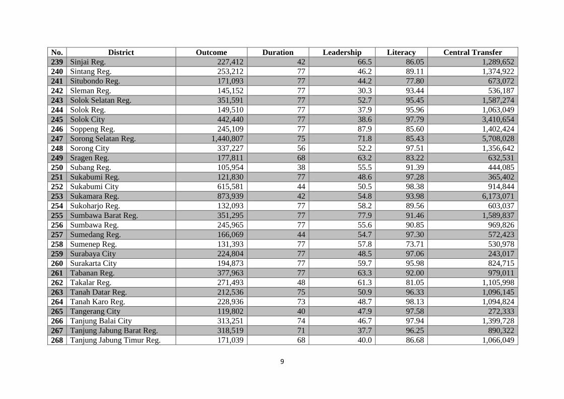
9
No. District Outcome Duration Leadership Literacy Central Transfer
239 Sinjai Reg. 227,412 42 66.5 86.05 1,289,652
240 Sintang Reg. 253,212 77 46.2 89.11 1,374,922
241 Situbondo Reg. 171,093 77 44.2 77.80 673,072
242 Sleman Reg. 145,152 77 30.3 93.44 536,187
243 Solok Selatan Reg. 351,591 77 52.7 95.45 1,587,274
244 Solok Reg. 149,510 77 37.9 95.96 1,063,049
245 Solok City 442,440 77 38.6 97.79 3,410,654
246 Soppeng Reg. 245,109 77 87.9 85.60 1,402,424
247 Sorong Selatan Reg. 1,440,807 75 71.8 85.43 5,708,028
248 Sorong City 337,227 56 52.2 97.51 1,356,642
249 Sragen Reg. 177,811 68 63.2 83.22 632,531
250 Subang Reg. 105,954 38 55.5 91.39 444,085
251 Sukabumi Reg. 121,830 77 48.6 97.28 365,402
252 Sukabumi City 615,581 44 50.5 98.38 914,844
253 Sukamara Reg. 873,939 42 54.8 93.98 6,173,071
254 Sukoharjo Reg. 132,093 77 58.2 89.56 603,037
255 Sumbawa Barat Reg. 351,295 77 77.9 91.46 1,589,837
256 Sumbawa Reg. 245,965 77 55.6 90.85 969,826
257 Sumedang Reg. 166,069 44 54.7 97.30 572,423
258 Sumenep Reg. 131,393 77 57.8 73.71 530,978
259 Surabaya City 224,804 77 48.5 97.06 243,017
260 Surakarta City 194,873 77 59.7 95.98 824,715
261 Tabanan Reg. 377,963 77 63.3 92.00 979,011
262 Takalar Reg. 271,493 48 61.3 81.05 1,105,998
263 Tanah Datar Reg. 212,536 75 50.9 96.33 1,096,145
264 Tanah Karo Reg. 228,936 73 48.7 98.13 1,094,824
265 Tangerang City 119,802 40 47.9 97.58 272,333
266 Tanjung Balai City 313,251 74 46.7 97.94 1,399,728
267 Tanjung Jabung Barat Reg. 318,519 71 37.7 96.25 890,322
268 Tanjung Jabung Timur Reg. 171,039 68 40.0 86.68 1,066,049

10
No. District Outcome Duration Leadership Literacy Central Transfer
269 Tanjung Pinang City 404,494 47 65.7 98.70 1,115,172
270 Tapanuli Tengah Reg. 280,281 71 57.3 93.85 919,724
271 Tapanuli Utara Reg. 266,626 36 52.3 97.60 1,278,088
272 Tapin Reg. 394,264 47 53.9 95.36 1,563,488
273 Tasikmalaya City 289,732 50 49.1 99.48 669,824
274 Tebo Reg. 147,293 67 28.0 96.48 1,042,657
275 Tegal Reg. 113,503 37 52.6 89.47 430,412
276 Teluk Bintuni Reg. 1,312,338 75 53.4 89.19 6,086,633
277 Teluk Wondama Reg. 2,061,491 75 67.9 79.65 8,837,747
278 Temanggung Reg. 137,895 41 57.8 94.48 593,268
279 Tidore Kepulauan City 429,259 77 55.4 97.30 2,723,163
280 Timor Tengah Selatan Reg. 136,255 36 29.6 79.47 910,651
281 Timor Tengah Utara Reg. 221,876 74 31.1 85.79 1,298,939
282 Toba Samosir Reg. 407,352 77 45.5 98.28 1,521,654
283 Tojo Una-Una Reg. 385,683 77 64.9 96.03 1,573,835
284 Toli-Toli Reg. 276,325 76 69.8 93.22 1,482,323
285 Tomohon City 321,433 77 54.0 99.24 2,360,989
286 Trenggalek Reg. 181,906 75 48.2 91.44 679,739
287 Tuban Reg. 130,384 67 64.5 85.00 468,446
288 Tulungagung Reg. 203,200 44 52.3 93.53 623,701
289 Wajo Reg. 257,647 38 48.7 86.95 896,516
290 Wakatobi Reg. 420,768 75 82.1 93.53 2,066,919
291 Way Kanan Reg. 105,360 77 62.9 94.89 796,314
292 Wonogiri Reg. 132,697 74 57.5 83.50 621,922
293 Wonosobo Reg. 176,068 74 65.3 91.16 558,699
294 Yapen Waropen Reg. 771,001 77 24.9 92.43 3,301,392
295 Yogyakarta City 342,936 60 63.6 97.16 907,514

11
Appendix 1.2: Fuzzy Set Scores
No. District Outcome Duration Leadership Literacy Central Transfer
1 Agam Reg. 0.06 1.00 0.53 0.94 0.14
2 Alor Reg. 0.52 0.00 0.74 0.26 0.61
3 Asmat Reg. 0.99 1.00 0.34 0.00 1.00
4 Balangan Reg. 0.71 1.00 0.64 0.94 0.66
5 Balikpapan City 0.34 0.67 0.83 0.99 0.01
6 Bandung City 0.01 0.00 0.61 1.00 0.01
7 Banggai Kepulauan Reg. 0.20 0.67 0.36 0.86 0.63
8 Banggai Reg. 0.22 0.67 0.81 0.75 0.53
9 Bangka Barat Reg. 0.69 1.00 0.64 0.68 0.46
10 Bangka Tengah Reg. 0.60 1.00 0.82 0.95 0.41
11 Bangka Reg. 0.50 0.00 0.75 0.98 0.15
12 Bangkalan Reg. 0.05 0.00 0.62 0.00 0.02
13 Bangli Reg. 0.56 1.00 0.62 0.00 0.37
14 Banjar Baru City 0.56 1.00 0.54 1.00 0.30
15 Banjar Reg. 0.29 1.00 0.47 0.84 0.06
16 Banjar City 0.84 0.00 0.62 0.98 0.40
17 Banjarmasin City 0.03 1.00 0.55 0.99 0.04
18 Banjarnegara Reg. 0.03 0.67 0.75 0.01 0.03
19 Bantaeng Reg. 0.41 0.00 0.79 0.00 0.46
20 Bantul Reg. 0.10 1.00 0.75 0.18 0.04
21 Banyumas Reg. 0.05 0.00 0.15 0.77 0.02
22 Banyuwangi Reg. 0.01 1.00 0.25 0.01 0.02
23 Barito Kuala Reg. 0.18 0.33 0.57 0.79 0.23
24 Barito Selatan Reg. 0.79 0.67 0.35 1.00 0.93
25 Barito Timur Reg. 0.69 0.00 0.52 0.99 0.97
26 Barito Utara Reg. 0.85 0.00 0.57 0.98 0.93
27 Barru Reg. 0.64 1.00 0.93 0.00 0.60
28 Batam City 0.07 0.67 0.50 1.00 0.01
29 Batang Reg. 0.04 0.67 0.54 0.09 0.03

12
No. District Outcome Duration Leadership Literacy Central Transfer
30 Batanghari Reg. 0.38 1.00 0.39 0.75 0.31
31 Batu City 0.01 0.33 0.37 0.93 0.28
32 Bau-bau City 0.53 0.33 0.69 0.42 0.79
33 Bekasi Reg. 0.01 0.33 0.53 0.79 0.01
34 Bekasi City 0.02 0.00 0.30 0.99 0.01
35 Belitung Timur Reg. 0.79 1.00 0.74 0.96 0.87
36 Belitung Reg. 0.78 0.00 0.69 0.97 0.64
37 Bengkayang Reg. 0.19 1.00 0.41 0.01 0.51
38 Bengkulu Selatan Reg. 0.77 0.00 0.79 0.84 0.77
39 Bengkulu City 0.03 0.33 0.60 1.00 0.30
40 Berau Reg. 0.97 1.00 0.68 0.98 0.62
41 Bima City 0.08 0.00 0.32 0.60 0.68
42 Binjai City 1.00 1.00 0.32 1.00 0.25
43 Bintan Reg. 0.72 1.00 0.63 0.96 0.19
44 Bitung City 0.18 1.00 0.72 1.00 0.56
45 Blitar Reg. 0.02 1.00 0.52 0.24 0.03
46 Blitar City 0.89 1.00 0.83 0.98 0.64
47 Blora Reg. 0.04 1.00 0.76 0.00 0.03
48 Boalemo Reg. 0.62 0.67 0.75 0.60 0.62
49 Bogor Reg. 0.02 0.00 0.51 0.83 0.01
50 Bogor City 0.01 0.00 0.57 0.99 0.01
51 Bojonegoro Reg. 0.04 0.33 0.70 0.00 0.02
52 Bone Bolango Reg. 0.65 1.00 0.71 0.98 0.68
53 Bone Reg. 0.05 0.00 0.70 0.00 0.06
54 Boven Digoel Reg. 0.98 1.00 0.41 0.38 1.00
55 Boyolali Reg. 0.08 1.00 0.67 0.02 0.04
56 Brebes Reg. 0.01 0.33 0.55 0.00 0.01
57 Bukittinggi City 0.09 1.00 0.41 1.00 0.85
58 Bulukumba Reg. 0.08 1.00 0.77 0.00 0.12
59 Bungo Reg. 0.51 0.67 0.27 0.97 0.28

13
No. District Outcome Duration Leadership Literacy Central Transfer
60 Buol Reg. 0.52 0.33 0.50 0.98 0.84
61 Buton Reg. 0.11 0.67 0.95 0.00 0.35
62 Cianjur Reg. 0.02 0.67 0.41 0.99 0.01
63 Cilacap Reg. 0.02 0.33 0.62 0.22 0.02
64 Cilegon City 0.43 1.00 0.56 0.99 0.06
65 Cimahi City 0.44 0.33 0.60 1.00 0.02
66 Cirebon Reg. 0.05 0.00 0.51 0.11 0.01
67 Dairi Reg. 0.22 0.00 0.46 1.00 0.33
68 Deli Serdang Reg. 0.02 0.00 0.46 0.99 0.02
69 Dharmas Raya Reg. 0.34 1.00 0.49 0.99 0.48
70 Dumai City 0.81 1.00 0.47 0.99 0.02
71 Ende Reg. 0.32 0.00 0.49 0.75 0.40
72 Enrekang Reg. 0.51 0.00 0.40 0.01 0.49
73 Fak-Fak Reg. 0.99 1.00 0.74 0.99 1.00
74 Gorontalo City 0.82 0.00 0.71 1.00 0.57
75 Gowa Reg. 0.02 1.00 0.85 0.00 0.04
76 Gresik Reg. 0.06 1.00 0.64 0.85 0.02
77 Grobogan Reg. 0.02 0.67 0.76 0.04 0.02
78 Gunung Kidul Reg. 0.05 1.00 0.62 0.00 0.06
79 Halmahera Barat Reg. 0.42 1.00 0.24 0.87 0.86
80 Halmahera Selatan Reg. 0.71 1.00 0.72 0.92 0.60
81 Hulu Sungai Selatan Reg. 0.78 0.00 0.54 0.91 0.50
82 Hulu Sungai Tengah Reg. 0.24 1.00 0.43 0.98 0.30
83 Hulu Sungai Utara Reg. 0.51 0.33 0.64 0.93 0.27
84 Humbang Hasundutan Reg. 0.38 1.00 0.64 0.99 0.62
85 Indragiri Hilir Reg. 0.05 0.00 0.19 0.99 0.03
86 Indragiri Hulu Reg. 0.19 1.00 0.48 0.98 0.07
87 Indramayu Reg. 0.03 1.00 0.80 0.00 0.01
88 Jambi City 0.07 0.00 0.30 1.00 0.06
89 Jayapura Reg. 0.82 0.67 0.69 0.38 1.00
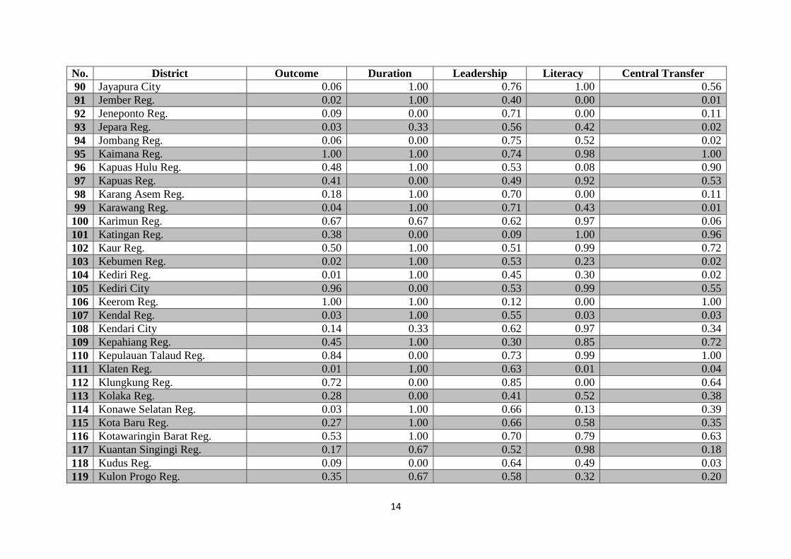
14
No. District Outcome Duration Leadership Literacy Central Transfer
90 Jayapura City 0.06 1.00 0.76 1.00 0.56
91 Jember Reg. 0.02 1.00 0.40 0.00 0.01
92 Jeneponto Reg. 0.09 0.00 0.71 0.00 0.11
93 Jepara Reg. 0.03 0.33 0.56 0.42 0.02
94 Jombang Reg. 0.06 0.00 0.75 0.52 0.02
95 Kaimana Reg. 1.00 1.00 0.74 0.98 1.00
96 Kapuas Hulu Reg. 0.48 1.00 0.53 0.08 0.90
97 Kapuas Reg. 0.41 0.00 0.49 0.92 0.53
98 Karang Asem Reg. 0.18 1.00 0.70 0.00 0.11
99 Karawang Reg. 0.04 1.00 0.71 0.43 0.01
100 Karimun Reg. 0.67 0.67 0.62 0.97 0.06
101 Katingan Reg. 0.38 0.00 0.09 1.00 0.96
102 Kaur Reg. 0.50 1.00 0.51 0.99 0.72
103 Kebumen Reg. 0.02 1.00 0.53 0.23 0.02
104 Kediri Reg. 0.01 1.00 0.45 0.30 0.02
105 Kediri City 0.96 0.00 0.53 0.99 0.55
106 Keerom Reg. 1.00 1.00 0.12 0.00 1.00
107 Kendal Reg. 0.03 1.00 0.55 0.03 0.03
108 Kendari City 0.14 0.33 0.62 0.97 0.34
109 Kepahiang Reg. 0.45 1.00 0.30 0.85 0.72
110 Kepulauan Talaud Reg. 0.84 0.00 0.73 0.99 1.00
111 Klaten Reg. 0.01 1.00 0.63 0.01 0.04
112 Klungkung Reg. 0.72 0.00 0.85 0.00 0.64
113 Kolaka Reg. 0.28 0.00 0.41 0.52 0.38
114 Konawe Selatan Reg. 0.03 1.00 0.66 0.13 0.39
115 Kota Baru Reg. 0.27 1.00 0.66 0.58 0.35
116 Kotawaringin Barat Reg. 0.53 1.00 0.70 0.79 0.63
117 Kuantan Singingi Reg. 0.17 0.67 0.52 0.98 0.18
118 Kudus Reg. 0.09 0.00 0.64 0.49 0.03
119 Kulon Progo Reg. 0.35 0.67 0.58 0.32 0.20

15
No. District Outcome Duration Leadership Literacy Central Transfer
120 Kuningan Reg. 0.05 0.00 0.54 0.98 0.03
121 Kutai Barat Reg. 0.95 0.67 0.53 0.98 0.82
122 Lamandau Reg. 0.84 0.00 0.65 0.99 1.00
123 Lamongan Reg. 0.03 1.00 0.66 0.02 0.02
124 Lampung Tengah Reg. 0.00 1.00 0.33 0.71 0.03
125 Landak Reg. 0.05 0.67 0.38 0.43 0.21
126 Langkat Reg. 0.03 0.00 0.31 0.99 0.03
127 Lebak Reg. 0.03 0.00 0.58 0.88 0.02
128 Lebong Reg. 0.35 1.00 0.44 0.93 0.87
129 Lembata Reg. 0.68 0.67 0.35 0.17 0.79
130 Limapuluh City Reg. 0.06 1.00 0.24 0.99 0.27
131 Lingga Reg. 0.96 1.00 0.32 0.06 0.76
132 Lombok Tengah Reg. 0.03 1.00 0.25 0.00 0.03
133 Lubuk Linggau City 0.32 0.00 0.90 0.99 0.24
134 Lumajang Reg. 0.02 0.00 0.43 0.00 0.02
135 Luwu Timur Reg. 0.67 1.00 0.83 0.49 0.17
136 Luwu Utara Reg. 0.57 1.00 0.78 0.51 0.19
137 Luwu Reg. 0.14 0.00 0.79 0.08 0.17
138 Madiun Reg. 0.05 0.00 0.63 0.00 0.05
139 Madiun City 0.63 0.00 0.70 0.98 0.57
140 Magelang Reg. 0.02 0.00 0.66 0.62 0.02
141 Magelang City 0.99 1.00 0.60 0.98 0.80
142 Magetan Reg. 0.13 0.00 0.72 0.06 0.07
143 Majalengka Reg. 0.04 0.00 0.38 0.90 0.03
144 Malang Reg. 0.01 1.00 0.28 0.03 0.01
145 Malang City 0.01 0.00 0.42 0.98 0.03
146 Mamuju Utara Reg. 0.18 1.00 0.62 0.02 0.73
147 Manado City 0.03 1.00 0.40 1.00 0.15
148 Mandailing Natal Reg. 0.05 1.00 0.75 1.00 0.12
149 Manggarai Barat Reg. 0.06 1.00 0.64 0.67 0.26

16
No. District Outcome Duration Leadership Literacy Central Transfer
150 Mappi Reg. 0.98 1.00 0.19 0.00 1.00
151 Maros Reg. 0.16 1.00 0.55 0.00 0.18
152 Medan City 0.11 1.00 0.33 1.00 0.01
153 Melawi Reg. 0.25 1.00 0.59 0.00 0.65
154 Merangin Reg. 0.07 0.00 0.07 0.89 0.27
155 Merauke Reg. 0.81 1.00 0.39 0.84 0.99
156 Metro City 0.82 1.00 0.63 1.00 0.64
157 Mimika Reg. 0.97 0.00 0.47 0.65 0.61
158 Minahasa Utara Reg. 0.12 1.00 0.53 1.00 0.54
159 Minahasa Reg. 0.04 0.33 0.72 1.00 0.31
160 Mojokerto Reg. 0.01 1.00 0.73 0.64 0.02
161 Mojokerto City 1.00 0.00 0.51 0.98 0.80
162 Morowali Reg. 0.59 0.33 0.55 0.87 0.80
163 Muara Enim Reg. 0.51 0.00 0.79 0.98 0.03
164 Muaro Jambi Reg. 0.13 0.67 0.43 0.98 0.11
165 Mukomuko Reg. 0.70 1.00 0.35 0.62 0.61
166 Murung Raya Reg. 0.83 0.00 0.48 1.00 1.00
167 Musi Banyuasin Reg. 0.59 0.67 0.92 0.99 0.01
168 Musi Rawas Reg. 0.11 1.00 0.91 0.95 0.08
169 Nganjuk Reg. 0.08 0.00 0.41 0.16 0.03
170 Ngawi Reg. 0.03 1.00 0.78 0.00 0.04
171 Ogan Ilir Reg. 0.04 1.00 0.73 0.99 0.07
172 Ogan Komering Ilir Reg. 0.05 0.00 0.77 0.93 0.06
173 OKU Selatan Reg. 0.04 1.00 0.66 0.98 0.07
174 OKU Timur Reg. 0.05 1.00 0.80 0.88 0.04
175 Ogan Komering Ulu Reg. 0.21 1.00 0.74 0.95 0.23
176 Pacitan Reg. 0.09 1.00 0.18 0.03 0.06
177 Padang Panjang City 1.00 0.00 0.55 0.99 1.00
178 Padang Pariaman Reg. 0.06 1.00 0.33 0.67 0.18
179 Padang Sidempuan City 0.39 0.33 0.65 1.00 0.47

17
No. District Outcome Duration Leadership Literacy Central Transfer
180 Padang City 0.02 0.00 0.39 1.00 0.06
181 Pagar Alam City 0.46 0.00 0.90 0.99 0.57
182 Palangkaraya City 0.06 0.00 0.58 1.00 0.65
183 Palembang City 0.02 0.00 0.81 0.99 0.02
184 Palopo City 0.77 0.00 0.74 0.89 0.65
185 Palu City 0.52 1.00 0.66 0.99 0.25
186 Pamekasan Reg. 0.04 0.00 0.60 0.00 0.03
187 Pandeglang Reg. 0.01 1.00 0.33 0.84 0.03
188 Pangkajene Kepulauan Reg. 0.39 1.00 0.40 0.00 0.22
189 Pariaman City 0.63 0.00 0.36 0.99 0.97
190 Parigi Moutong Reg. 0.08 0.00 0.79 0.23 0.13
191 Pasaman Barat Reg. 0.07 1.00 0.56 0.82 0.13
192 Pasaman Reg. 0.23 1.00 0.42 0.99 0.30
193 Pasir Reg. 1.00 1.00 0.78 0.98 0.05
194 Pasuruan Reg. 0.02 0.00 0.11 0.05 0.01
195 Pasuruan City 0.58 1.00 0.21 0.92 0.38
196 Pati Reg. 0.05 0.67 0.64 0.01 0.02
197 Payakumbuh City 0.82 0.33 0.44 0.99 0.83
198 Pekalongan Reg. 0.10 0.67 0.49 0.07 0.03
199 Pekalongan City 0.26 1.00 0.65 0.95 0.13
200 Pekan Baru City 0.01 0.67 0.48 1.00 0.01
201 Pelalawan Reg. 0.03 0.67 0.23 0.94 0.06
202 Pematang Siantar City 0.54 1.00 0.60 1.00 0.41
203 Pesisir Selatan Reg. 0.09 1.00 0.34 0.87 0.16
204 Pinrang Reg. 0.13 0.00 0.68 0.32 0.17
205 Pohuwato Reg. 0.60 1.00 0.70 0.51 0.77
206 Polewali Mandar Reg. 0.08 0.00 0.69 0.00 0.12
207 Ponorogo Reg. 0.08 1.00 0.26 0.02 0.04
208 Pontianak City 0.13 0.00 0.43 0.81 0.06
209 Poso Reg. 0.50 1.00 0.54 0.98 0.84

18
No. District Outcome Duration Leadership Literacy Central Transfer
210 Prabumulih City 0.70 0.00 0.92 0.98 0.40
211 Probolinggo Reg. 0.02 0.00 0.76 0.00 0.02
212 Probolinggo City 0.66 0.00 0.91 0.02 0.27
213 Pulang Pisau Reg. 0.49 0.00 0.79 0.99 0.91
214 Purbalingga Reg. 0.05 1.00 0.90 0.46 0.03
215 Purwakarta Reg. 0.03 0.00 0.30 0.96 0.02
216 Purworejo Reg. 0.08 1.00 0.40 0.26 0.06
217 Rejang Lebong Reg. 0.30 1.00 0.45 0.84 0.39
218 Rembang Reg. 0.17 1.00 0.81 0.20 0.05
219 Rokan Hulu Reg. 0.10 0.67 0.70 0.98 0.02
220 Salatiga City 0.92 0.67 0.73 0.90 0.43
221 Samarinda City 0.05 1.00 0.41 0.99 0.02
222 Sambas Reg. 0.09 0.67 0.47 0.23 0.11
223 Sampang Reg. 0.02 0.33 0.47 0.00 0.02
224 Sanggau Reg. 0.10 0.00 0.24 0.03 0.23
225 Sarolangun Reg. 0.13 0.67 0.55 0.89 0.36
226 Sawahlunto Sijunjung Reg. 0.16 1.00 0.26 0.51 0.49
227 Sawahlunto City 0.98 0.00 0.49 0.98 0.99
228 Sekadau Reg. 0.12 1.00 0.30 0.07 0.49
229 Selayar Reg. 0.55 1.00 0.90 0.37 0.81
230 Seluma Reg. 0.12 1.00 0.41 0.75 0.54
231 Semarang City 0.02 1.00 0.40 0.96 0.02
232 Serdang Bedagai Reg. 0.03 1.00 0.27 0.99 0.04
233 Seruyan Reg. 0.41 0.00 0.73 0.97 0.96
234 Sidenreng Rappang Reg. 0.31 0.00 0.54 0.00 0.33
235 Sidoarjo Reg. 0.02 1.00 0.53 0.99 0.01
236 Sikka Reg. 0.34 0.00 0.76 0.01 0.21
237 Simalungun Reg. 0.03 1.00 0.52 0.98 0.06
238 Singkawang City 0.62 0.33 0.17 0.02 0.54
239 Sinjai Reg. 0.18 0.00 0.78 0.00 0.42

19
No. District Outcome Duration Leadership Literacy Central Transfer
240 Sintang Reg. 0.26 1.00 0.43 0.03 0.51
241 Situbondo Reg. 0.07 1.00 0.39 0.00 0.05
242 Sleman Reg. 0.04 1.00 0.19 0.65 0.03
243 Solok Selatan Reg. 0.58 1.00 0.55 0.93 0.62
244 Solok Reg. 0.04 1.00 0.29 0.96 0.21
245 Solok City 0.73 1.00 0.30 0.99 0.99
246 Soppeng Reg. 0.23 1.00 0.94 0.00 0.52
247 Sorong Selatan Reg. 1.00 1.00 0.84 0.00 1.00
248 Sorong City 0.56 0.33 0.54 0.99 0.50
249 Sragen Reg. 0.07 0.67 0.73 0.00 0.04
250 Subang Reg. 0.02 0.00 0.60 0.20 0.02
251 Sukabumi Reg. 0.03 1.00 0.47 0.99 0.01
252 Sukabumi City 0.91 0.00 0.51 1.00 0.12
253 Sukamara Reg. 0.98 0.00 0.59 0.76 1.00
254 Sukoharjo Reg. 0.03 1.00 0.65 0.04 0.03
255 Sumbawa Barat Reg. 0.58 1.00 0.89 0.21 0.62
256 Sumbawa Reg. 0.24 1.00 0.60 0.13 0.15
257 Sumedang Reg. 0.06 0.00 0.59 0.99 0.03
258 Sumenep Reg. 0.03 1.00 0.64 0.00 0.03
259 Surabaya City 0.17 1.00 0.47 0.98 0.01
260 Surakarta City 0.10 1.00 0.67 0.96 0.09
261 Tabanan Reg. 0.63 1.00 0.73 0.32 0.16
262 Takalar Reg. 0.34 0.33 0.70 0.00 0.25
263 Tanah Datar Reg. 0.14 1.00 0.52 0.97 0.24
264 Tanah Karo Reg. 0.18 1.00 0.48 0.99 0.24
265 Tangerang City 0.03 0.00 0.46 0.99 0.01
266 Tanjung Balai City 0.51 1.00 0.44 0.99 0.52
267 Tanjung Jabung Barat Reg. 0.52 1.00 0.28 0.97 0.11
268 Tanjung Jabung Timur Reg. 0.07 0.67 0.32 0.00 0.22
269 Tanjung Pinang City 0.67 0.33 0.76 1.00 0.25

20
No. District Outcome Duration Leadership Literacy Central Transfer
270 Tapanuli Tengah Reg. 0.38 1.00 0.63 0.73 0.13
271 Tapanuli Utara Reg. 0.32 0.00 0.54 0.99 0.41
272 Tapin Reg. 0.66 0.33 0.57 0.92 0.61
273 Tasikmalaya City 0.42 0.33 0.48 1.00 0.05
274 Tebo Reg. 0.04 0.67 0.16 0.97 0.20
275 Tegal Reg. 0.02 0.00 0.55 0.04 0.02
276 Teluk Bintuni Reg. 1.00 1.00 0.56 0.03 1.00
277 Teluk Wondama Reg. 1.00 1.00 0.79 0.00 1.00
278 Temanggung Reg. 0.04 0.00 0.64 0.84 0.03
279 Tidore Kepulauan City 0.71 1.00 0.60 0.99 0.95
280 Timor Tengah Selatan Reg. 0.03 0.00 0.18 0.00 0.12
281 Timor Tengah Utara Reg. 0.16 1.00 0.20 0.00 0.43
282 Toba Samosir Reg. 0.68 1.00 0.42 1.00 0.59
283 Tojo Una-Una Reg. 0.64 1.00 0.75 0.96 0.62
284 Toli-Toli Reg. 0.36 1.00 0.82 0.60 0.57
285 Tomohon City 0.53 1.00 0.57 1.00 0.90
286 Trenggalek Reg. 0.08 1.00 0.47 0.21 0.05
287 Tuban Reg. 0.03 0.67 0.75 0.00 0.02
288 Tulungagung Reg. 0.12 0.00 0.54 0.67 0.04
289 Wajo Reg. 0.28 0.00 0.48 0.00 0.12
290 Wakatobi Reg. 0.70 1.00 0.92 0.67 0.83
291 Way Kanan Reg. 0.02 1.00 0.72 0.88 0.08
292 Wonogiri Reg. 0.03 1.00 0.64 0.00 0.04
293 Wonosobo Reg. 0.07 1.00 0.76 0.17 0.03
294 Yapen Waropen Reg. 0.97 1.00 0.13 0.41 0.99
295 Yogyakarta City 0.57 0.67 0.73 0.99 0.12