the relationship between nominal wage and ... - bank of mexico
TRANSCRIPT
Banco de México
Documentos de Investigación
Banco de México
Working Papers
N° 2020-20
The Relat ionship Between Nominal Wage and PriceFlexibil i ty: New Evidence
December 2020
La serie de Documentos de Investigación del Banco de México divulga resultados preliminares detrabajos de investigación económica realizados en el Banco de México con la finalidad de propiciar elintercambio y debate de ideas. El contenido de los Documentos de Investigación, así como lasconclusiones que de ellos se derivan, son responsabilidad exclusiva de los autores y no reflejannecesariamente las del Banco de México.
The Working Papers series of Banco de México disseminates preliminary results of economicresearch conducted at Banco de México in order to promote the exchange and debate of ideas. Theviews and conclusions presented in the Working Papers are exclusively the responsibility of the authorsand do not necessarily reflect those of Banco de México.
Diego SolórzanoBanco de México
Huw DixonCardiff University

The Relat ionship Between Nominal Wage and PriceFlexibi l i ty: New Evidence*
Abstract: The frequencies at which prices and wages are adjusted, interpreted as price and wageflexibility, are key elements in workhorse models used for policy analysis. Yet, there is little evidenceregarding the relationship between these two sources of nominal rigidities. Using two large and highlydisaggregated price and wage microdata sets, this paper provides evidence that the industries changingmore frequently wages reset prices more often. Once the frequency of wage adjustments is accountedfor, the share of labor costs becomes less relevant in explaining the frequency of price changes, callingfor a reinterpretation on previous findings that the labor share is a robust determinant of the frequency ofprice adjustments. The results in this study have implications for New Keynesian models'microfoundations, as their predictions have proven to be sensitive to the nominal rigidities assumptions.Keywords: Nominal Stickiness; Micro Price Data; Micro Wage Data; Frequency of AdjustmentsJEL Classification: E31, J31, C26
Resumen: La frecuencia en la que los precios y salarios se ajustan, interpretada como la flexibilidadde precios y salarios, es un elemento central en modelos comúnmente utilizados para el análisis depolíticas económicas. Sin embargo, existe poca evidencia sobre la relación entre estas fuentes derigideces nominales. Utilizando bases de microdatos de precios y salarios desagregadas, el presentedocumento provee evidencia de que las industrias que ajustan más frecuentemente salarios son aquellasque cambian sus precios más a menudo. Asimismo, una vez que se controla por la frecuencia de cambiode salarios, la proporción de costos de mano de obra se vuelve menos relevante en explicar la frecuenciade ajustes de precios, haciendo importante reinterpretar los resultados de estudios previos queencuentran que el costo de mano de obra es un determinante robusto de la frecuencia de cambio deprecios. Los resultados de este estudio tienen implicaciones para los microfundamentos de los modelosNeo-Keynesianos, pues sus predicciones han mostrado ser sensibles a los supuestos sobre rigidecesnominales.Palabras Clave: Rigideces Nominales; Microdatos Precios; Microdatos Salarios; Frecuencia de Cambios
Documento de Investigación2020-20
Working Paper2020-20
Diego So lórzano †
Banco de MéxicoHuw Dixon ‡
Cardiff University
*We would like to thank Alejandrina Salcedo, Josué Cortés, Erwan Gautier, Engin Kara, Patrick Minford, aswell as seminar participants at the University of Warwick, Cardiff-Business School, National Bank of Belgium,Lietuvos Bank and Banco de México for their useful comments. This paper has benefited from Banco de México'sEconLab initiative. All errors remain ours. † Dirección General de Investigación Económica. Email: [email protected]. ‡ Cardiff Business School. Cardiff University. Email: [email protected].

1 Introduction
Does wage flexibility drive price flexibility? Do industries resetting wages more fre-
quently change prices more often? Based on two separate and highly disaggregated worker
and product-level datasets from Mexico, we look at the fraction of wage and price adjust-
ments at industry-level and study them under a panel structure. To the authors’ knowledge,
this is the first paper to use such extensive quantitative datasets to link together wage changes
and price adjustments. Our panel of industries includes information from prices and wages
in Mexico from 2011 to 2018 and allows addressing unobserved heterogeneity at the indus-
try level. We interpret the flexibility of wage and price adjustment in terms of the observed
proportion of goods and workers that receive a price or wage change.1
Our findings suggest that price flexibility is indeed affected by wage flexibility. There is
a positive effect of the frequency of wage adjustments on the frequency of price changes. On
average, an increase of 1 p.p. in the fraction of workers receiving a wage adjustment in the
year is translated into a 1.2 p.p. raise in the frequency of price changes. We alleviate po-
tential endogeneity issues by using an instrumental variable approach. The instrument is the
share of minimum wage workers in a given industry. Intuitively, as minimum wage workers
normally receive only one wage adjustment in the year, the share of minimum wage workers
affects wage flexibility and price flexibility only through the proportion of wage adjustments.
Using this as an instrument we are able to avoid attributing causal status to wage frequency
that might derive from a third factor influencing both price and wage frequencies.
The majority of small to medium scale New Keynesian DSGE models use the Calvo
(1983) framework. The Calvo framework assumes price- and wage-setters face a constant
probability of adjustment. As there is a continuum of price- and wage-setters, the probability
of adjustment is mapped as the fraction of price- and wage-setters adjusting their prices and
wages, respectively, period by period.2 However, there is no theoretical mechanism for the1The literature review by Klenow et al. (2010) highlights numerous studies using the frequency of price
adjustments as a measure of price flexibility. This is the norm throughout this paper.2The Calvo framework assumes price- and wage-setters adjust their prices and wages to its optimal level.
Hence, it does not account for the size of adjustment. We follow this approach in the paper and focus on the
1

frequency of wage changes to influence price-setting in these models. Following Erceg et al.
(2000), most models assume that there is a continuum of labor types which are combined by
aggregation to be a single labor input to firms in all sectors/industries, in the same way the
intermediate monopolistically competitive goods are combined into a single output.3 Hence,
there is no industry-specific link between wages and prices. Whilst this may be a convent
theoretical simplification, in practice wages and much of the labor input are industry specific.
We link wages and prices in our two datasets.
We are able to explore the extent to which downward nominal rigidities in wages might
be greater than for prices. On the one side, employees dislike receiving wage cuts which
prevents employers from decreasing wages.4 On the other side, it is easier for price-setters
to engage in sales strategies which would lead to roughly the same number of price increases
and decreases. Hence, concerns arise in whether the positive relationship is driven by in-
dustries with more frequent wage increases but with prices jumping around reference prices.
Therefore, we estimate our model focusing on the frequency of wage and price increases
only. The main qualitative results are confirmed for this case. Furthermore, since our dataset
reports whether a price is considered a sale/end-of-sale price, we are able to filter out sales-
related price changes. We also find evidence that the frequency of wage changes increases
the frequency of price changes when sales are excluded.
Peneva (2011), Vermeulen et al. (2012) and Alvarez et al. (2006) document an inverse
relationship between the frequency of price adjustments and the share of labor costs for the
US and some EU economies. As Klenow et al. (2010) summarises, labor-intensive sectors
adjust prices less frequently, potentially because wages adjust less frequently than prices.
When we do not control for the frequency of wage changes, our data supports this result.
However, once the frequency of wage adjustment is included in the econometric framework,
labor share becomes statistically insignificant. In contrast, the effects of frequency of wage
fraction of price and wage changes only.3Smets and Wouters (2003) or Galı (2015) provide a detailed description of models featuring monopolistic
competition in both the goods and labor markets using a-la-Calvo price- and wage-setting.4See, for instance, Le Bihan et al. (2012), Barattieri et al. (2014) and Sigurdsson and Sigurdardottir (2016).
Employers might also be impeded to incur in wage cuts by local regulations. That is the case for Mexicanemployers.
2

adjustment are statistically significant in our different specifications. Therefore, our results
might call for a reinterpretation of previous findings in the literature.
Our IV estimation using the share of minimum wage workers as instrument relies on the
fact that minimum wage workers normally receive only one wage adjustment in the year,
while non-minimum wage employees generally receive more than one wage revision in the
year. Our instrument would fail to generate exogenous variation on the frequency of wage
changes when, for instance, both minimum wage and non-minimum wage workers receive
roughly the same number of adjustments on the same year. In fact, that was the case for
minimum wage workers in certain areas in Mexico in 2012, 2015 and 2017.5 Hence, our
benchmark specification does not consider these years.
The literature on price and wage setting using microdata has been growing rapidly in the
last decade. On the one hand, the price literature has reached a consensus about the great
degree of heterogeneity on price flexibility across different sectors/industries in the economy.
See, among others, Bils and Klenow (2004), Alvarez et al. (2006), Dixon and Tian (2017).
Likely determinants of such sectoral heterogeneity have been studied by the Inflation Persis-
tent Network (IPN). One of the conclusions of IPN’s research was that wages were among the
most important factors determining the timing to reset prices.6 In the same line, and impor-
tantly for this research, Peneva (2011) and Vermeulen et al. (2012) find that industries with
a higher share of labor costs in total costs make less frequent price adjustments, potentially
resulting from the fact that wages adjust less frequently than prices.7 Our analysis empiri-
cally assesses whether wage flexibility contributes to price flexibility. To our knowledge, no
previous study has systematically investigated this relationship. The analysis that is closest5Prior 2012, there were three different minimum wage rates in the Mexican economy. In 2012 and 2015,
there were extemporaneous minimum wage adjustments (in addition to the annual increase) affecting welldefined geographical areas catching up with the highest minimum wage rate. By late 2015 there was a singleminimum wage rate nation-wide. Moreover, the 2018 minimum wage increase was brought forward to late2017. Thus, 2017 also saw two minimum wage adjustments.
6These conclusions lead to IPN’s follow up project: Wage Dynamic Network.7This is “Fact 10: Price changes are linked to wage changes” in the Handbook of Monetary Economics by
Klenow et al. (2010). Citing work by Peneva (2011) and Vermeulen et al. (2012), this stylised fact is reachedby looking at the (indirect) relationship between price changes and wage changes via the share of labor costs.Our paper uncovers quantitatively if price changes are driven by wage changes for the first time to the best ofour knowledge.
3

to our approach, and makes the most progress in studying jointly price and wage setting, is
Druant et al. (2012) from the Wage Dynamic Network (WDN). The authors find firms tend
to concentrate wage changes in a specific month, mostly January in a majority of European
countries, and that prices change when wages change in general. The main weakness, how-
ever, in Druant et al. (2012) is the descriptive approach they follow due to the qualitative data
from categorial questionnaires they have at hand. In contrast, we use nearly ten years of quan-
titative product- and worker-level data, which is then analysed using a panel IV estimation at
industry level.
On the other hand, studies by Sigurdsson and Sigurdardottir (2016) and Le Bihan et al.
(2012) are important references analysing wage-setting determinants. Importantly for this
study, Gautier et al. (2016) documents that high-wage workers tend to receive more frequent
wage adjustments than low-wage workers in France. We find a similar pattern in Mexico’s
labor market and exploit this critical labor market characteristic in our IV strategy.
The contribution of our results to the nominal rigidities literature is twofold. First, we
assess the role of wage flexibility driving price flexibility. Despite the fact wages greatly con-
tribute to the encompassed value added in final prices, wage flexibility is yet to be analysed
as a determinant of price flexibility in a formal econometric setting.8 Second, it provides evi-
dence that enriches the design and calibration of microfounded New Keynesian DSGE mod-
els with nominal rigidities. Research by Carvalho (2006), Kara (2015), Dixon and Le Bihan
(2012) and Solorzano and Dixon (2019) highlight that properly modelling the heterogeneity
on the frequency of price and wage adjustments (as observed in microdata) alters aggregates’
dynamics in DSGE models. Indeed, Solorzano and Dixon (2019) poses the idea that a positive
relationship between the two nominal frictions (price and wage rigidities) would not be trivial
for aggregate dynamics. They show that a multi-sector economy, calibrated under a positive
relationship between prices and wages, exacerbates the real side effects of nominal shocks.9
8As mentioned above, Druant et al. (2012) use a narrative approach to highlight that managers in EU firmsconsider the timing of wage revisions, among other factors, for the timing of price adjustments.
9Solorzano and Dixon (2019) devote greater effort on presenting the multi-sector DSGE and the implicationsof the likely positive relationship of prices and wages. They show, as motivation for their work, some descriptiveevidence of this relationship by fitting a cross-section of industries using a standard OLS estimation. Instead,this paper assesses the causal relationship of wage flexibility on price flexibility using a panel IV framework.
4

This paper is organised as follows. Section 2 discusses the empirical strategy followed in
the paper and describes the data. Section 3 reports results. Finally, Section 4 concludes.
2 Econometric Framework
The section below describes the empirical strategy, as well as the data we rely on as-
sessing whether wage flexibility results in price flexibility. We start by presenting the panel
specification. Then, we explain why endogeneity issues might arise and the instrumentation
behind, and we finish detailing some descriptive statistics from our datasets.
2.1 Empirical Strategy
In line with papers exploiting the industry-level heterogeneity to study potential determi-
nants of the frequency of price adjustments, we regress the frequency of price adjustments on
the frequency of wage adjustments and further industry characteristics.10 Our framework is
FreqPriceAdjk,t = ↵ + �1FreqWagesAdjk,t + �2Xk,t + �k + �t + "k,t (1)
where subscripts k and t represent industry and year respectively. FreqPriceAdjk,t is the
frequency of price adjustments and FreqWagesAdjk,t is the frequency of wage adjustments.
Described in greater detailed below, FreqPriceAdjk,t (FreqWagesAdjk,t) is calculated as
the average in year t of the fraction of monthly price (wage) changes in industry k. Xk,t are
a set of time-varying industry characteristics. These industry characteristics are the share of
labor costs, a proxy aiming at controlling on how easy it is for certain sectors to adjust their10See, among others, Alvarez et al. (2006), Alvarez et al. (2010), Cornille and Dossche (2006) for similar
econometric approaches regressing frequency of price changes on industry characteristics. The literatureusually calculates industry characteristics using statistics drawn from Input-Output tables. The closest theliterature gets is to include the share of labor costs. No previous study has investigated the role of wagerigidities on price rigidities, mainly due to data limitations, and we are able to uncover this relationship byanalysing two independent price and wage datasets at industry level.
5

labor costs and energy intensity.11 �k is a set of industry fixed effects controlling for the size
of price adjustment and unobserved heterogeneity at industry level; and �t is a set of time
fixed effects addressing common shocks to all industries at different points in time.
As presented in great detail in the data subsection, the frequency of wage adjustments is
calculated using information from formal workers only. Hence, our benchmark results should
be seen as the effect of formal workers’ wage changes on price adjustments.12
Estimating the econometric framework specified in Equation 1 using OLS would produce
biased results due to two main reasons likely to be present in our context. First, our specifi-
cation might suffer from reverse causality. For instance, suppose households set their wages
only after price-setters have decided the fraction of new prices in the economy. Second, there
is an omitted variable bias concern. Failing to address this issue might attribute causal status
to the wage adjustment frequency that might derive from a third factor influencing both price
and wage frequencies. For instance, one can think of a productivity shock affecting both
price and wage frequencies of adjustments.13 As long as the omitted variable is temporal
over our sample and affecting all industries, time fixed effects in our specification should
ameliorate this problem to a great extent. Alternatively, industry fixed effects accounts for
industry-specific shocks if they prevail throughout our panel.
We address both sources of endogeneity by instrumenting the frequency of wage adjust-
ment with the share of Minimum Wage (MW) workers by industry in a year. The intuition
on the instrument and tests regarding its relevance is as follows. On the relevance aspect, the
share of MW workers is likely to have a predictive power over the frequency of wage adjust-
ment because, historically, these workers have received only one wage increase per year.14
11The proxy on how easy it is for certain sectors to adjust their labor costs is defined as the standard deviationof the detrended and seasonally adjusted labor force in industry k over year t. See Subsection 2.2 for more onthe calculation of this covariate.
12Note that informality, along with other input shares in the production function, is unlikely to vary substan-tially over our sample years. Therefore, industry fixed effects might ameliorate the bias stemming from the lackof informal workers in our sample. Nonetheless, in one of the robustness checks, we go to the data and include acovariate controlling for the degree of informal workers. The qualitative conclusions do not change whatsoever.
13Imagine a natural disaster or a fiscal stimulus generating greater demand for some or all industries’ output,which in turn boost resetting prices and wage revisions.
14Notable exceptions are 2012, 2015 and 2017 when minimum wage rates were adjusted more than oncewithin a single year.
6

Such sole increase implies a frequency of wage adjustment of 8.3% or 112 for minimum wage
workers, where the 12 in the denominator reflects the fact that the panel is formed of yearly
averages calculated using monthly observations. As the share of minimum wage workers
increases in industry k, FreqWagesAdjk,t would converge to 8.3%. On the contrary, as min-
imum wage workers decreases in industry k, FreqWagesAdjk,t would rise from 8.3%. The
stylised fact that minimum wage workers tend to receive less frequent wage adjustments than
non-minimum wage workers is supported by our data and discussed in great detail below.
This intuition can be summarised in an analytical expression where FreqWagesAdjk,t
is seen as the weighted average of the frequency of wage adjustment of those earning the
minimum wage and those earning above the minimum wage, FreqWagesAdjMWk,t and
FreqWagesAdjNoMWk,t , respectively. That is,
FreqWagesAdjk,t = ↵MWk,t FreqWagesAdjMW
k,t +�1� ↵MW
k,t
�FreqWagesAdjNoMW
k,t
= ↵MWk,t
�FreqWagesAdjMW
k,t � FreqWagesAdjNoMWk,t
�...
...+ FreqWagesAdjNoMWk,t
where ↵MWk,t , the share of minimum wage workers at industry k in year t, is our proposed
instrument. Thus, the relationship between the instrument ↵MWk,t and the endogenous vari-
able FreqWagesAdjk,t reveals the gap between non-minimum wage and minimum wage
frequencies of adjustments,
@FreqWagesAdjk,t@↵MW
k,t
= FreqWagesAdjMWk,t � FreqWagesAdjNoMW
k,t (2)
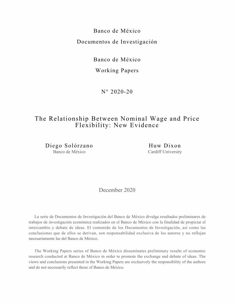
We are able to shed further light in the relevance of our instrument on FreqWagesAdjk,t
by looking at the data. First, if FreqWagesAdjMWk,t ⇡ 1
12 < FreqWagesAdjNoMWk,t , we
might expect @FreqWagesAdjk,t@↵MW
k,tto have a negative sign. Indeed, Figure 1a illustrates a down-
ward slopping relation between FreqWagesAdjk,t and ↵MWk,t using all k-t observations in our
panel.15 Moreover, Figure 1b shows that FreqWagesAdjMWk,t (depicted as red diamonds) are,
15These statistics are described and computed in Subsection 2.2 in great detail.
7

Figure 1: Frequency of Wage Adjustments and Share of MW Workers.0
1020
30Fr
eque
ncy
of W
age
Adju
stm
ents
(%)
0 20 40 60 80 100Share of MW Workers (%)
(a) Industry-Year observations
010
2030
Freq
uenc
y of
Wag
e Ad
just
men
ts (%
)
0 20 40 60 80 100Share of MW Workers (%)
FWANoMWk,t
FWAMWk,t
Fitted FWAk,t
(b) Industry-Year observations by income.
Note: The two panels plot the frequency of wage adjustment (vertical axis) and the share of minimum wageworkers (horizontal axis) per industry per year. Panel 1a, left, depicts the pool of observations in our panel ofindustries. Each diamond represents one industry in one year. The height for each diamond is the frequency ofwage adjustment, whereas the width is the share of minimum wage workers. Panel 1b, right, disaggregates thefrequency of wage adjustments into the frequency of wage adjustments for non-minimum wage workers (bluediamonds) and minimum wage workers (red diamonds). Thus, each industry is represented by two diamondssharing the same width, the share of minimum wage worker, which is a within industry characteristic.
in general, below FreqWagesAdjNoMWk,t (depicted as blue diamonds). Furthermore, Table
1 reports aggregates arising from Figure 1b. Importantly, the difference between the first
and second rows of column one shows that FreqWagesAdjMWk,t is roughly 6 p.p. less than
FreqWagesAdjNoMWk,t . The fact that workers in higher income deciles receive more frequent
wage adjustments than workers in the lower deciles is not something unique to the Mexican
economy. Gautier et al. (2016) have documented similar patterns for French workers. In sum,
our data supports the idea of a negative sign in Equation 2.
Second, if FreqWagesAdjMWk,t ⇡ FreqWagesAdjNoMW
k,t , Equation 2 implies that our
instrument would no longer be relevant. Table 1 highlights that FreqWagesAdjNoMWk,t , on
average, is about 50% greater than FreqWagesAdjMWk,t , where the latter is normally dictated
by the annual (single) MW update. Figure 1b also makes this case, FreqWagesAdjNoMWk,t
is nearly half FreqWagesAdjMWk,t . Thus, years in which MW workers receive more than
one wage adjustment might lead to FreqWagesAdjMWk,t ⇡ FreqWagesAdjNoMW
k,t , there-
fore, both terms on the right hand side in Equation 2 would cancel out, leading to a potential
weak instrument estimation. There are three years in our sample when that might be the case:
2012, 2015 and 2017.
8

Table 1: Average Frequency of Wage Adjustment by Income and Share of MW WorkersFrequency of Frequency of Share ofAdjustments Increases Workers
Mean Std. Dev Mean Std. Dev Mean(1) (2) (3) (4) (5)
Less than 1.5 MW 10.96 5.10 9.45 4.30 36.63More or equal than 1.5 MW 17.04 4.60 13.57 3.58 63.37Overall 15.05 4.97 12.23 3.79 100.00Note: This table shows the frequency of wage adjustment by income level. Each entry in the table iscalculated, first, at industry level and then as unweighted averages across industries. More specifically,workers in a given industry are split into two bins: bin one contains those earning less than 1.5minimum wages, while bin two considers those earning more than 1.5 minimum wages. Then, thefraction of wage changes is calculated for each bin for all industries. Finally, in order to calculate theaverage frequency of wage adjustment of those earning less than 1.5 minimum wages, for instance,we compute the unweighted average of bins one across industries. Similarly, the standard deviation ofthose earning less than 1.5 minimum wages is calculated as the unweighted standard deviation of thefrequency of wage adjustments of bins one across industries. The last row follows the same steps justdescribed but without splitting workers by income level. Note that the minimum wage level changesover time and had different rates per region. Special care is taken in order to classify who was aboveand below the 1.5 minimum wage threshold depending the worker’s location (e.g. there were three MWregions in early 2011 but only one MW region by late 2018) and year of observation (e.g. the MW didnot remain flat over our sample period). The dataset reports wages from 2011 to 2018. For more detailson the wage dataset, see Subsection 2.2.
The first two of them, 2012 and 2015, are related to a policy intervention unifying the
minimum wage rate nation-wide.16 As the first episode in 2012 affected only a handful of
locations (about 2% of Mexican municipalities), FreqWagesAdjk,t did not exhibit any dra-
matic change relative to previous years. See Figure 2 and the lack of any abrupt variation
in 2012. The second episode in 2015 affected more than 95% of Mexican municipalities.
A humped shape in 2015 can be seen in Figure 2 as a result of the unification policy. The
two minimum wage adjustments in 2015 would lead to weak instrumentation as Equation 2
shows. Thus, we discard 2015 from our benchmark panel IV specification.
The third year where there are two MW adjustment on the same year and special attention
is required is 2017. In 2017, the annual minimum wage increase corresponding to 2018 was
brought forward to November 2017. Again, due to the double minimum wage increase in
2017, @FreqWagesAdjk,t@↵MW
k,tmight be close to zero. As the second MW revision was fairly late
16Before 2012, there were three different minimum wage zones in Mexico. A new policy unifying MWrates in Mexico took place in two independent episodes (2012 and 2015) affecting two independent geographicregions.
9

in the year and prices are not adjusted promptly, it is likely that wage changes are reflected
onto prices in 2018. Thus, instead of simply dropping out 2017 (as with 2015), we address
this issue by imputing the late 2017 minimum wage increase as if it would have happened in
2018. Observed and imputed values are shown in Figure 2.17 Nonetheless, we report results
using both observed and imputed data in Section 3.
Regarding the contemporaneous price flexibility resulting from wage flexibility assumed
in Model 1, and not allowing any lasting effect i.e. lags, two main reasons arise. On the one
hand, dealing with serial correlation arising from lagged covariates would further shortened
the panel. On the other hand, wage adjustments tend to happen early in the year and goods’
prices tend to accommodate shocks fairly quickly, while service prices are also adjusted early
in the calendar year.18 Thus, we believe the contemporaneous relationship asserted in the
panel reflects well the wage effects on prices.
With respect to the nature of "k,t in Equation 1, we assume the error terms are correlated
within broad industry categories. This assumption comes from the fact that industries either
have overlapping production lines and/or some products act as substitutes between industries
(e.g. food-related industries). Described in greater detail in the following subsection, the (70)
industries in our final sample are clustered into six broad categories. However, inference from
the cluster-robust variance matrix estimator can be misleading when there are only six clus-
ters and when they are not homogeneous enough in size.19 As inference using cluster-robust
variance estimators can lead to over-rejection when the number of clusters is small, we con-17The imputation was made by recoding the last two months of 2017 as the first two months of 2018
by industry. In order to rebalance the number of observations in 2017 industries’ averages, the average offrequency of wage adjustments for the last two months from 2011 to 2016 was calculated by industry andimputed as the last two months in 2017. Notice that, while the imputation strategy addresses the issue in theidentification strategy regarding double minimum wage adjustments in 2017, it creates a problem for the 2018data: substituting the observed first two months in 2018 with the last two months of 2017, wage adjustmentsreceived by workers in, say, January 2018 are neglected (more likely from non-minimum wage workers). Thus,the observed and imputed values of 2018 lack from the wage adjustments of minimum and non-minimum wageworkers, respectively. That is reflected in the similar values solid and dashed lines exhibit in 2018 in Figure 2.These statistics are described at great detail in Subsection 2.2.
18See Sigurdsson and Sigurdardottir (2016) for wages and Nakamura and Steinsson (2008) for prices.19The six broad categories are (i) food-related goods, (ii) non-food goods, (iii) household-related services,
(iv) education services, (v) healthcare and recreational services, and (vi) other services. The cluster offood-related goods encompasses nearly a quarter of industries.
10

duct inference in our benchmark model using clustered wild bootstrap-t procedure.20 Wild
bootstrap testing tends to be more conservative yielding improvements in the performance of
cluster-robust methods in small samples. Following Cameron et al. (2008) and Djogbenou
et al. (2019) recommendation with less than 10 clusters, we use Webb weights. The number
of bootstrap replications is 999 in all regressions.
Figure 2: Frequency of Wage Adjustment.Unweighted yearly average across industries.
1314
1516
1718
Freq
uenc
y of
Wag
e Ad
just
men
t (%
)
2010 2012 2014 2016 2018Sample Years
Data Imputed
Note: This figure shows the aggregate frequency of wage adjustments using data from the 70 industries inour final sample. For more on the industries in our sample, see Subsection 2.2. The aggregate yearly figuresare calculated as the unweighted average of frequency of wage adjustments across industries. Industries’frequencies of wage adjustments in a given year are defined as the fraction of monthly wage changes withinan industry. The solid line plots the frequency of wage adjustments as observed directly from the data; whilethe dashed line shows the resulting frequency once 2017 and 2018 were imputed. The imputation was madeby recoding the last two months of 2017 as the first two months of 2018 by industry. In order to rebalance thenumber of observations in the 2017 averages, the average of frequency of wage adjustments for the last twomonths from 2011 to 2016 was calculated by industry and imputed as the last two months in 2017.
2.2 Data
For this paper we use highly disaggregated data for both prices and wages, as well as
some aggregate data from national account statistics. In this section we first describe the
price and wage datasets, we then address the measures of price and wage flexibility and its20Particularly, we use the wild restricted efficient residual bootstrap developed by Davidson and MacKinnon
(2010) and Roodman et al. (2019) for panel IV specifications. The clustered wild bootstrap is implemented bymultiplying the residuals from the original linear model by random weights in order to construct bootstrap sam-ples with dependent variables that are related to the independent variables by the same linear model. Inferenceusing wild bootstrap is not new in economics. See, for instance, Busso et al. (2013) and Zimmerman (2014).
11

merge at industry level, finally we present the industry characteristics used as controls in our
econometric framework.
Regarding prices, we use CPI microdata at product level. That is, we observe individual
prices, as well as some product characteristics. Importantly, the dataset reports whether the
price is categorised as sale or not.
This dataset comes from Instituto Nacional de Estadıstica y Geografıa (INEGI), Mex-
ico’s National Statistical Agency, and contains the universe of prices considered in the CPI
survey. A number of considerations are needed in the dataset before we can use it in our
econometric framework.
First, the CPI survey takes place in Mexico twice a month (fortnightly). In order to have
the same frequency of observation as our wage data, which is monthly, we opt to use the
second fortnight observation of the month. Taking monthly price averages could have seen
as alternative option. However, as Campbell and Eden (2014) suggest, time averages make a
single price change look like two consecutive smaller changes. Thus, and without loss of gen-
erality, the second fortnight price of the month is taken as our primarily unit of observation
for prices.
Second, the price dataset includes a variable classifying each individual price observation
into a single product category.21 Product categories are then grouped into 4-digit industries
using the North American Industry Classification System (NAICS). It is worth mentioning
that the cross-walk from product category to 4-digit industry is made publicly available by
INEGI.22 Thus, our panel’s unit of observation is at industry level. The use of industry-
level data has been extensively used by the nominal rigidities literature. For instance, see
Dhyne et al. (2006) for a review on this literature analysing determinants of price rigidities
at industry level. The analysis across industries allows us to merge the large price and wage
micro-datasets in a transparent and neat way. Each dataset serves different purposes, contains
different variables and the data is gathered and reported by different institutions. Although
one can think of carrying out the analysis at retail and/or brand level, the variables in our21Product categories are known by INEGI (in Spanish) as Genericos.22See INEGI (2018) for more.
12

datasets do not provide enough information for merging the large number of individual eco-
nomic agents across datasets. Nonetheless, working at industry level is in line with much of
the literature on nominal rigidities as highlighted above.
Third, few industries are dropped out from our analysis. These are industries in the non-
core component of the Mexican CPI. We opt to neglect them because of three main reasons
stemming from the design of the price survey. First, some prices are reported as composite
prices and, thus, we are unable to disentangle what price component actually changed (e.g.
holiday expenses are reported as the sum of transportation plus accommodation). Second,
some prices are regulated and do not obey market conditions, particularly labor market dy-
namics (e.g. toll road fees). Third, the quality of some goods is not constant over time and
might be reflected into prices (e.g. fresh fruit and vegetables near the end of their season).
If we have had accurate price statistics for these industries (neither composite, nor regulated,
nor quality driven), our identification strategy would have carried forward. As of them may
be labor intensive, they would have added value to our analysis. In total, 70 out of the 283
original price categories, which translates into 16 out of the 86 industries, are neglected from
the analysis.
Forth, prices in some industries are more likely to enter into sales strategies i.e. prices
jumping around a reference price. Sales strategies would lead to a disproportionally high fre-
quency of adjustment, without necessarily reflecting prices’ ability to mirror their new (wage-
induced) marginal cost. Fortunately, our dataset classifies prices as normal, sale, exiting sale.
Thus, we are able to calculate metrics of price flexibility using all price observations, which
we call “posted prices”, and using sales-free prices only, which we call “normal prices”.
Regarding wages, we use microdata at worker level from Instituto Mexicano del Seguro
Social (IMSS), Mexico’s Social Security Institute. That is, we observe individual workers’
wages, as well as some job characteristics and demographics. Importantly for our analysis,
we are able to observe the industry where the worker is employed.
This dataset contains the census of IMSS affiliated workers. A number of considerations
are needed in the dataset before it is ready for our econometric framework.
13

First, the dataset contains the last daily wage in a given month for each worker as reported
by her employer. We compare this observation month to month for calculating the frequen-
cies of wage adjustments. A strength of our data relative to other social security or income
surveys datasets is that IMSS’s wages are reported as standardised base salaries. The base
salary includes not only the monthly wage but pro-rata bonuses stipulated in the worker’s
labor contract. For instance, Mexican workers receive an end-of-year bonus in December
by law. Thus, seasonal bonuses would not lead to temporal wage adjustments biasing our
measures of wage flexibility.
Second, IMSS reports the industry at which the worker is employed. Importantly, IMSS
uses its own industry classification system which share broad similarities to NAICS. We ad-
dress the NAICS and IMSS merge in great detail below. In terms of the industry composition,
the price data reports fewer industries than the wage data as it only reports final goods, while
the wage data offers observations from intermediate goods (e.g. mining industry). Hence, we
only consider workers in industries included in both price and wage datasets.
Third, we focus on the wages of workers who remain in the same job (job-stayers). Al-
though few studies have considered job-switching wage changes, we opt to keep our wage
rigidity measures as comparable as possible to our price analysis. That is, comparing the
wage level of the same worker (item) at the same firm (retailer) relative to its wage (price)
in the previous period, with presumably the same job (item) characteristics. If an individual
worker has two or more jobs, he or she appears more than once in the dataset. We consider
such cases as different wages as each wage (earned by the same worker) contributes to the
wage flexibility of its own industry.
Forth, workers are categorised as permanent or temporal according to IMSS regulation.
Our analysis only considers permanent workers. The decision not to include temporal work-
ers is based on the fact that they are normally seasonal hires and/or upon completion of a
special task (e.g. extra chores over the Christmas season). Also, wage adjustments to perma-
nent workers is the one that matters for price determination presumably as temporal workers
14

do not develop a job history in the firm.23
Having presented the features in the price and wage datasets, we move on to discuss the
differences between prices’ NAICS and wages’ IMSS classification system.24 Both classifi-
cation systems are 4-digits and a great number of them share the same names. We identify
three different cardinalities when merging industries: (i) one NAICS to one IMSS, (ii) more
than one NAICS to one IMSS, and (iii) one NAICS to more than one IMSS. For the second
case, price observations in multiples NAICS were pooled (unweighted) in order to calculate
a single industry figure. For the last case, efforts were made to break down one NAICS code
into more disaggregated codes in order to maximise the number of 1-to-1 industry relation-
ships between NAICS and IMSS. Breaking down NAICS is possible since the price data
includes product descriptions. One example are NAICS’s “Beverages” and IMSS’s “Beer”,
“Other alcoholic beverages”, “Soft drinks”. Using the product category variable in the price
data, we disaggregate NAICS into three industries. The benefit is twofold. First, it provides a
more accurate relationship between producers’ wages and final prices. Second, it allows us to
maximise the number of industries in our sample. As we discuss into great detail in Section 3,
much of our results are explained by industry heterogeneity and not by time variation, hence
the importance of disaggregating as much as possible the number of industries in our sample.
All in all, our panel of 70 industries encompasses data from 11 million of price quotes
(around 60% of the CPI’s expenditure weights) and 1,150 million wage observations. These
industries constitute 40% of Mexico’s GDP.
In order to calculate the key variables in this study, the frequencies of price and wage ad-
justments, we follow standard procedures in the literature (e.g. Bils and Klenow (2004);
Nakamura and Steinsson (2010); Dixon and Tian (2017) for prices; and Le Bihan et al.
(2012); Sigurdsson and Sigurdardottir (2016) for wages). We compute these variables in
two steps. In the first step, we define a dummy variable at product (worker) level that takes
the value of one if the product’s price (worker’s wage) changed in a given month, and zero23Future work should look into whether temporal workers’ wages remain flat over the contract or not; or
study whether the duration of wage/employment spells is drastically different between permanent and temporalworkers. This is out of the scope of the present analysis.
24We use the NAICS published in 2013.
15

otherwise. We consider the product’s price (worker’s wage) changed if and only if a good
(worker) was observed in the current and immediate previous month and the price (wage) was
not the same relative to its value in the previous month. In order to control for measurement
errors, only log variation above 0.1 p.p. were taken as an actual change. Bear in mind these
dummy variables are defined at product and worker level and observed at monthly frequen-
cies. In the second step, we calculate the fraction of dummy variables reporting price and
wage changes by industry per year. Equivalently, the second step can be seen as taking the
yearly average by industry of the product and worker dummy variables.
Specifically, we have the following expressions for calculating our measures of flexibility:
FreqPriceAdjk,t =
Pi2k,m2t 1 if pi,m 6=pi,m�1P
i2k,m2t 1 if pi,m & pi,m�1 observed and not sales
FreqPostedAdjk,t =
Pi2k,m2t 1 if pi,m 6=pi,m�1P
i2k,m2t 1 if pi,m & pi,m�1 observed
FreqWageAdjk,t =
Pi2k,m2t 1 if wi,m 6=wi,m�1P
i2k,m2t 1 if wi,m & wi,m�1 observed
where the subscript i stand for an individual product or worker, k for industries, m and t for
month and year, respectively.
Hence, FreqPriceAdjk,t, FreqPostedAdjk,t and FreqWageAdjk,t are the yearly aver-
ages of monthly frequencies of normal price, posted price and wage adjustments, respectively,
for industry k in year t. The decision to have t, years, as the benchmark observation frequency
in our panel is taken as some prices (e.g. services) and wages do not change every month.
Little monthly variation from wages, sluggish and heterogeneous labor costs pass-through
across industries, in addition to the small number of industries would lead to little power in
our statistical inference.
Moreover, wages are known to be more downward rigid than prices and, while prices in
16

some industries are also downward rigid (e.g. services’ prices), price drops are more often
observed in some industries (e.g. goods’ prices). Negative demand shocks are a good exam-
ple when this scenario might arise. Wage-setters are unable to negatively adjust their wage
level, while price-setters are able to decrease their price level. In such case, we would observe
an apparent disconnection between price and wage flexibility. By contrast, both wages and
prices can be positively adjusted in the presence of positive demand shocks. In such case, we
would observe a strong link between price and wage flexibility. Hence, in order to limit the
effects on the downward asymmetries between wages and prices, a set of results studying the
frequency of price and wage hikes is also analysed. Thus, we calculate:
FreqPriceAdj+k,t =
Pi2k,m2t 1 if pi,m>pi,m�1P
i2k,m2t 1 if pi,m & pi,m�1 observed and not sales
FreqPostedAdj+k,t =
Pi2k,m2t 1 if pi,m>pi,m�1P
i2k,m2t 1 if pi,m & pi,m�1 observed
FreqWageAdj+k,t =
Pi2k,m2t 1 if wi,m>wi,m�1P
i2k,m2t 1 if wi,m & wi,m�1 observed
2.3 Stylized Facts
Table 2 reports descriptive statistics by industry. More particularly, each column reports
industries’ averages across years for the frequency of adjustments. This is known as the
within-variation in the panel data literature. For instance, column 1 is calculated as:
FreqPriceAdjk =
PTt=1 FreqPriceAdjk,t
T
and column 2 shows FreqPostedAdjk. Columns 3 and 4 report industry averages using nor-
mal and posted price increases. Columns 5 and 6 provides the frequency of wage adjustments
and the frequency of wage hikes only, respectively.
17

The frequency of price adjustment vis-a-vis the frequency of wage adjustment at industry
level presented in Table 2 is noteworthy as there is no other study making this comparison in
the nominal rigidities literature. Table 2 lists the complete set of industries in the panel under
study. In line with the price literature (e.g. Nakamura and Steinsson (2008)) but less so with
the wage literature (e.g. Sigurdsson and Sigurdardottir (2016)), there is substantial amount
of heterogeneity across industries in both the frequency of price change and in the frequency
of wage adjustments. On the one hand, the frequency of price changes for normal prices goes
from 36% (Motor Vehicle Manufacturing) to 2% (Parking Services). The between industries’
standard deviation regarding the frequency of price changes is 9.78%. On the other hand, the
frequency of wage adjustment bounce between 25% (Other Household Appliances Manufac-
turing) and 4% (Private Households Services). The between industries’ standard deviation
regarding the frequency of wage adjustments is 4.62%.
Table 3 reports descriptive statistics by years. That is, it presents the yearly average across
unweighted industry observations. For instance, the first row of statistics is calculated as:
FreqPriceAdjt =
PKk=1 FreqPriceAdjk,t
K
Hence, the first two rows of statistics in Table 3 provide the bloc corresponding to normal
(sales-free) prices. The second set of two rows are calculated using posted prices, whereas
the last two rows report yearly statistics from the wage data.
Compared to the between industry variation illustrated in Table 2, the variation across
years reports considerably less variation. In fact, the standard deviation of the frequency of
price adjustments and the frequency of wage changes are 1.06% and 1.12%, respectively.
Thus, our results are mainly explained by industry variation and not by time variation.
It is also worth comparing the frequency of price changes and the frequency of wage
adjustments in Mexico relative to other economies. Regarding posted prices, the mean is
20.43% in Mexico, while in the US is 19.3% according to Bils and Klenow (2004) and in
France 19% as reported by Dixon and Le Bihan (2012). The average frequency of adjustment
18

for normal prices in Mexico is 15.02%, nearly doubles that of the US 8.9% as calculated by
Nakamura and Steinsson (2008) but similar to the UK 14% according to Dixon and Tian
(2017). With respect to wages, Mexico’s frequency of wage changes is 15.05%, while for the
US and France is 9.9% and 14.7%, respectively, as reported by Barattieri et al. (2014) and
Le Bihan et al. (2012). Thus, the Mexican economy is fairly similar to the US, France and
the UK in terms of price rigidities. For wages, on the other hand, Mexico seems closer to
France than to the US.
Having presented the panel’s within- and between-variation, Figure 3 plots the pool of
observations in our panel for the different measures of price and wage flexibility. For in-
stance, Panel 3a depicts all k-t observations, where each diamond represents one industry in
a given year, the height indicates its frequency of price adjustment and its wide reflects its
frequency of wage adjustment. Panel 3b illustrates the relationship between the frequency of
posted price adjustments (vertical axis) and the frequency of wage changes (horizontal axis).
The second row of panels in Figure 3 follows the same idea but illustrating all observations
when considering only price and wage hikes.
Few interesting stylised facts arise from Figure 3. First, in all four panels, there is a
non-negligible number of observations below the 45% degree line. It implies that it is not
uncommon observing years in which industries reset more frequently their wages than their
prices. This stylised fact serves as evidence debunking the idea that wages are, in general,
more rigid than prices. This is specially true for Panel 3c, which takes into account sales on
the price data and the asymmetric downward rigidity between prices and wages. Our scatters
plots show otherwise. As this study is the first merging price and wage rigidities, we could
not find any reference point for other economies or if this is an idiosyncratic stylised fact for
the Mexican economy.
Second, there is greater heterogeneity on the price flexibility side than in the wage flexibil-
ity as discussed when presenting Table 2. The dispersion in the vertical axis for the different
panels is greater than the dispersion over the horizontal axes. Barattieri et al. (2014) hints at
less dispersion on the wage flexibility side relative to the dispersion of price flexibility for the
19

US. However, the authors reach this conclusion by comparing the dispersion of frequencies
of price changes across industries as reported in Bils and Klenow (2004) and their disper-
sion of the frequency of wage adjustments across different types of jobs (and not industries).
We are the first to provide quantitative evidence using a consistent dimension of comparison,
industries.
2.4 Industry Characteristics
For computing the industry characteristics labor costs, energy intensity and ease to adjust
labor force, represented as Xk,t in Equation 1, we use data from the KLEMS framework,
provided by INEGI, and the IMSS dataset.25 Published every year using national account
statistics, KLEMS is an informative tool on the productivity of factor inputs. Due to the
methodology employed in KLEMS, INEGI is able to provide an approximation on the indus-
tries’ costs structures. For consistency, we use the costs structures reported at 4-digit NAICS
and take them to the industry classification discussed above. Since the share of service inputs
is highly labor intensive (e.g. distribution costs), we compute our proxy for the share of labor
costs as the sum of labor and services shares. The industries reporting the largest and lowest
share of labor costs are Private Household Services (100%) and Real State Related Activities
(7%), respectively. Energy intensity is drawn directly from KLEMS’ energy (E) component.
The industry reporting the largest share of energy usage is Petroleum Products Manufactur-
ing (80%). Private Household Services (0%) is the least energy intensive industry. Lastly,
the ease to adjust labor force comes from the IMSS dataset. It is calculated as the standard
deviation of the (log) number of workers (detrended and seasonally adjusted) by industry per
year. On the one hand, Apparel Knitting Products is, on average, the industry with the most
volatile labor force (1.4). On the other hand, Grain Mill Products is the one exhibiting less
variation in their labor force (0.002) in our industry sample.
Finally, the share of minimum wage workers, which serves as our instrument for Equa-
tion 1, comes from the IMSS dataset. It is defined as the proportion of permanent workers25KLEMS stands for capital (K), labor (L), energy (E), materials (M) and services (S).
20

that receive less than 1.5 times the minimum wage prevailing at the time and region for a
given industry. There are two main reasons why we decide not to use the fraction of workers
earning the binding minimum wage. First, only a very small fraction of workers receive the
existing minimum wage. Presumably, since employers cannot report smaller wages than the
existing minimum wage by law, the reservation wage across industries is above the mini-
mum wage. Hence, the fraction of workers earning exactly one minimum wage is small and
with little heterogeneity across industries. Second, workers’ characteristics of those earning
the minimum wage and those earning just above the minimum wage might be very simi-
lar, including the wage-setting behaviour. Adding workers earning just above the minimum
wage in FreqWageAdjNoMWk,t would weaken the relationship between the endogenous vari-
able, FreqWageAdjk,t, and the instrument, ↵MWk,t , as shown in Equation 2. In other words,
FreqWageAdjNoMWk,t would get closer to FreqWageAdjMW
k,t if workers earning just above
the minimum wage were included to the former. Because of the above, the 1.5 threshold
gives a clear cut between the wage dynamics exhibited by minimum wage earners and non-
minimum wage earners. Robustness checks (not reported) using a 1.1 threshold do not change
the qualitative results whatsoever.
21

Table 2: Frequencies of Price and Wage Adjustments by IndustryPrices Wages
All Hikes All HikesIndustries Normal Posted Normal Posted
(1) (2) (3) (4) (5) (6)Median 13.80 17.41 9.77 11.34 15.14 12.26Mean 15.62 20.43 10.91 12.77 15.05 12.23Std. Dev. 9.78 13.05 6.10 7.19 4.62 3.32Accounting, Tax Prep and Payroll Services 3.10 3.48 3.00 3.30 11.46 9.86Activities Related to Real Estate 3.69 3.86 3.37 3.45 11.62 10.61Alcoholic Beverage Mfg 22.05 30.75 14.30 17.91 14.65 12.09Animal Food Mfg 32.41 40.83 21.03 24.45 15.27 12.77Animal Slaughtering and Processing 34.69 43.62 23.51 26.83 14.95 12.31Apparel Knitting Mills 8.93 13.26 6.17 8.11 16.81 13.70Automotive Repair and Maintenance 5.11 5.85 4.27 4.53 8.89 7.91Bakeries and Tortilla Mfg 16.48 23.04 11.86 14.58 11.41 9.69Batteries and Other Electrical Equipment Mfg 18.01 23.21 12.03 13.81 19.13 14.25Beer Mfg 18.55 23.38 13.55 15.33 19.58 13.52Child Day Care Services 3.62 3.62 3.54 3.54 9.24 8.49Coffee Product Mfg 25.87 35.49 16.89 20.63 11.79 9.89Commercial and Service Ind Machinery Mfg 7.81 14.21 5.18 7.41 20.42 16.49Confectionery Product Mfg 26.56 36.07 17.26 20.98 18.04 14.70Converted Paper Product Mfg 29.96 38.59 18.96 22.03 16.58 13.03Cutlery Product Mfg 13.60 18.81 10.04 12.26 17.03 13.25Dairy Product Mfg 31.07 41.45 20.04 24.15 16.51 13.27Death Care Services 4.80 5.52 4.20 4.41 8.91 7.96Dry-cleaning and Laundry Services 4.93 5.39 4.43 4.60 12.01 10.82Electric Lighting Equipment Mfg 14.01 18.33 8.81 10.88 20.00 15.69Footwear Mfg 8.99 12.16 6.71 7.98 8.25 6.88Fruit and Vegetable Preserving Food Mfg 29.25 39.94 18.64 22.74 16.72 13.41Full and Limited-Service Restaurants 10.79 11.78 9.39 9.77 11.28 10.01General Medical and Surgical Services 3.96 4.07 3.54 3.57 7.19 6.69Glass and Glass Product Mfg 12.07 16.91 8.90 11.09 19.89 15.22Grain Milling 34.55 43.80 21.04 24.64 14.59 12.84Grain Processed Food 35.59 49.90 22.43 27.48 16.03 13.97Ground Passenger Transportation 9.38 9.86 8.40 8.62 10.24 9.39Hand tool Product Mfg 21.98 28.82 14.58 17.10 14.54 12.12Household Appliances Mfg 20.74 33.08 14.37 19.25 22.59 17.20Household Furniture and Kitchen Cabinet Mfg 21.35 34.02 14.78 19.69 12.11 10.29Magnetic and Optical Media Reprod and Mfg 6.32 9.85 4.14 5.53 22.63 17.53Medical Equipment and Supplies Mfg 10.70 13.34 7.65 8.63 22.50 17.96Medical and Diagnostic Laboratories 4.98 6.21 4.23 4.66 11.89 9.48Misc Musical Instruments, Toys and Sport Eq Mfg 11.81 15.97 7.99 9.63 18.24 14.69Miscellaneous Candles and Others Mfg 13.31 17.46 9.17 11.10 11.63 8.94Miscellaneous Jewelry and Others Mfg 9.64 13.70 6.98 8.69 10.54 8.47Miscellaneous Stationary Mfg 13.60 16.41 9.59 10.48 23.56 17.85Miscellaneous Wood Products Mfg 15.51 21.36 10.20 12.48 10.60 9.14Motion Picture and Video Industries 9.86 10.69 8.71 9.04 13.03 10.76Motor Vehicle Mfg 35.91 38.67 26.32 26.76 23.97 18.56Motor Vehicle Parts Mfg 12.86 14.22 9.74 10.06 23.49 17.91Newspaper, Periodical and Book Publishers 5.63 5.90 4.60 4.67 11.08 9.21Nightclubs, Pubs and Canteens 4.15 4.34 3.59 3.66 13.91 11.29Non-alcoholic Beverage Mfg 17.51 24.14 12.64 15.47 16.98 13.98Offices of Dentists 4.09 4.54 3.56 3.75 10.35 8.34Oilseed Milling 35.25 45.66 21.44 25.38 19.00 14.49Other Amusement and Recreation Industries 4.46 4.89 3.72 3.86 15.01 11.93Other Chemical Product and Preparation Mfg 11.04 12.75 7.77 8.31 19.95 16.86Other Electrical Equipment Mfg 17.46 19.98 13.57 14.43 18.68 15.42Other Food Mfg 21.30 30.49 14.45 18.17 10.88 9.05Other Furniture Related Product Mfg 19.01 30.38 13.26 17.65 20.21 15.92Other Household Appliances Mfg 14.12 22.85 9.82 13.64 24.54 18.98Other Leather and Allied Product Mfg 9.66 14.72 6.59 8.82 15.33 12.11Other Transportation Equipment Mfg 14.41 20.10 10.48 12.41 15.34 11.87Parking Related Services 1.88 1.87 1.71 1.70 10.45 8.92Perfumes and Cosmetics Mfg 17.96 25.69 11.66 14.93 15.54 12.70Personal Care Services 3.22 3.66 2.91 3.07 6.02 5.87Personal and Household Goods Repair 9.58 13.45 6.72 8.25 8.54 7.26Pesticide and Fertilizer Mfg 30.84 38.86 19.19 21.91 12.48 10.11Petroleum Products Mfg 14.42 17.38 10.58 11.60 14.47 12.22Pharmaceutical and Medicine Mfg 26.49 29.81 18.52 19.34 19.00 15.23Plastics Product Mfg 10.47 14.19 7.41 8.94 16.95 13.41Private Households Services 2.97 2.98 2.72 2.72 4.22 4.08Rubber Product Mfg 19.38 26.20 13.58 15.71 14.59 11.44Seafood Product Preparation and Packaging 28.02 38.24 17.58 21.56 13.22 10.75Soap and Cleaning Compound Mfg 29.39 39.01 18.23 21.65 16.81 14.19Textile Furnishings Mills 9.72 14.51 6.88 9.03 15.53 12.53Tobacco Mfg 15.06 15.08 14.45 14.45 19.49 15.92Water Supply Services 17.65 17.66 16.80 16.81 15.39 12.65Note: This table lists the complete set of industries in our panel (70). Columns report industries’ frequencies of adjustment averagedacross time. Averages are calculated using data from 2011 to 2018. Column 1 to column 6 present the frequency of normal priceadjustments, posted price changes, normal price hikes, posted price increases, wage adjustments and wage increases, respectively.Median, mean and standard deviation are unweighted moments across industries.
22

Table 3: Frequencies of Price and Wage Adjustments by Year
Frequency of Adjustments 2011 2012 2013 2014 2015 2016 2017 2018 Median Mean Std. Dev.
Normal PricesAll Changes 16.29 15.01 14.01 15.27 14.62 15.84 16.96 16.93 15.56 15.62 1.076Hikes Only 11.33 10.72 9.395 10.64 10.11 11.16 12.42 11.55 10.94 10.91 0.926
Posted PricesAll Changes 20.79 19.78 19.19 20.63 19.78 20.82 21.75 20.67 20.65 20.43 0.801Hikes Only 12.95 12.55 11.52 12.74 12.20 12.99 14.11 13.08 12.85 12.77 0.748
WagesAll Changes 14.16 14.25 14.54 14.68 15.93 15.21 17.40 14.23 14.61 15.05 1.122Hikes Only 11.35 11.43 11.87 11.84 13.09 12.29 14.63 11.33 11.86 12.23 1.133
Note: This table reports descriptive statistics on the frequencies of adjustments by years. It presents years’ averages across unweighted industryobservations. That is, for a given year t, the average value of the frequency of adjustment across industries in year t is calculated. There are70 industries in our sample. The first two rows of statistics provide the bloc corresponding to normal prices. The second set of two rows arecalculated using posted prices, whereas the last two rows report wage statistics. Median, mean and standard deviation are unweighted momentsacross years.
3 Results
Table 4 reports estimates of regressing the frequency of normal price adjustments on the
frequency of wage changes plus industry and year fixed effects. The first three columns
present standard OLS estimates, whereas the latter three offer the results when the frequency
of wage adjustment is instrumented with the share of minimum wage workers. Bear in mind
the frequency of normal price adjustments is calculated filtering out sales prices.
Within each of the OLS and IV set of results, Table 4 shows the coefficients using three
different time samples following the arguments presented in Subsection 2.1.26 The coeffi-
cient in column 1 is calculated using years when only one minimum wage adjustment was
observed. Historically, in Mexico there is normally only one minimum wage adjustment in
the year. Consequently, the time restriction used in column 1 is under the title “Standard”.
The coefficient in column 2, titled “Data”, is obtained using observations from 2013 until26Using years with more than one minimum wage adjustment might lead both terms on the right hand side
of Equation 2 to cancel out and resulting in a non-relevant instrument. See Subsection 2.1 for more.
23

Figure 3: Frequencies of Adjustments.One observation per industry per year.
010
2030
4050
60Fr
eq N
orm
al P
rice
Adju
stm
ents
(%)
0 10 20 30 40 50 60Freq Wage Adjustments (%)
SectorsMedianMean45º
(a) Normal Prices and Wages. All Changes.
010
2030
4050
60Fr
eq P
oste
d Pr
ice
Adju
stm
ents
(%)
0 10 20 30 40 50 60Freq Wage Adjustments (%)
SectorsMedianMean45º
(b) Posted Prices and Wages. All Changes.
010
2030
4050
60Fr
eq N
orm
al P
rice
Incr
ease
s (%
)
0 10 20 30 40 50 60Freq Wage Increases (%)
SectorsMedianMean45º
(c) Normal Prices and Wages. Hikes Only.
010
2030
4050
60Fr
eq P
oste
d Pr
ice
Incr
ease
s (%
)
0 10 20 30 40 50 60Freq Wage Increases (%)
SectorsMedianMean45º
(d) Posted Prices and Wages. Hikes Only.
Note: The four panels plot the pool of observations in our panel for the different measures of price and wageflexibility. In all panels, each diamond represents one observation per industry per year. The height indicatesthe frequency of price adjustment and the width reflects the frequency of wage adjustment per industry peryear. Panel 3a depicts the relationship between the frequency of price adjustments (vertical axis) and thefrequency of wage changes (horizontal axis). Panel 3b illustrates the frequency of posted price adjustments andthe frequency of wage changes. Panel 3c compares the frequency of price increases and the frequency of wagehikes. Panel 3d presents the frequency of posted price increases and the frequency of wage hikes.
24

2018. Bear in mind that by using the full time span, the years with more than one minimum
wage adjustment (2015 and 2017) or no adjustment (2018) are included in the sample. As
discussed in great detail in Section 2, attempts were made to impute the 2018 observations
using data from late 2017. Column 3, under the title “Imputed”, reports the calculated coef-
ficient using the 2017 and 2018 imputed data. The same time specifications are repeated in
columns 4 to 6 but calculated via IV estimation.
Using standard years with one minimum wage adjustment, OLS estimates in Table 4
show a positive point estimate of 0.359. This result suggests a positive relationship between
price and wage flexibility. Note, however, point estimates are statistically insignificant. OLS
estimates including the whole time span as observed from the data are considerable lower
and even with a negative sign, -0.011. This coefficient is not only statistically insignificant
but also less precise than the coefficient using only standard years as shown by their p-value.
The third column in Table 4 tells a similar story than column 2 with a coefficient closer to
zero, -0.007. Hence, imputing seems to have little payoff in order to use more recent data.
In order to address any potential bias in our OLS estimates arising from endogeneity, we
look into the panel IV approach for critically studying whether wage flexibility causes price
flexibility. Columns 4 to 6 reporting the panel IV results assert the story told in columns 1
to 3 using an OLS framework. The different order of magnitudes confirm our endogeneity
concerns presented in Section 2. We come back to this issue after discussing the IV results.
Firstly, the coefficient of our variable of interest, the frequency of wage adjustment, is
positive and statistically significant when years with multiple minimum wage revisions are
excluded from the model (column 4). This is a key result in our research. The coefficient can
be interpreted as, for a 1 p.p. increase in the frequency of wage adjustments, it increases price
flexibility, in the form of the frequency of price adjustments, by 1.223 p.p. The first stage in
this specification also exhibits a statistically significant and negative sign as expected from
Equation 2. The F-statistic, around 30, provides some support that we do not have a problem
of weak identification between the instrument and the endogenous regressor. Moving into
estimates without imputations in 2017 and 2018, column 5, the point estimate of 0.812 is
25

smaller and less precise than employing standard years only. Nonetheless, it contrasts with
its OLS counterpart from column 2 by remaining above zero. Regarding column 6, imputing
2017 and 2018 observations, the coefficient close to unity, 1.071, but statistically insignifi-
cant. Also, note that the first stage coefficients in column 5 and column 6 are smaller than
in column 4, and thus, less precise second stages. We attribute this effect to the years with
atypical minimum wage adjustment policies in such years which dampens our instrument’s
identification strategy.
The differences between OLS and IV estimates in Table 4 are indicative of the poten-
tial endogeneity problems discussed in Section 2. However, the downward bias is somewhat
counterintuitive to the obvious omitted variable candidate for which our regression cannot
control for: a productivity shock. After a productivity shock, more frequent wage revisions
are expected as the wage level rises. Likewise for prices due to the greater demand for goods
and services. Thus, a productivity shock would affect both price and wage frequencies of
adjustments resulting in an upward biased OLS estimation.
One way to reconcile the downward bias found in Table 4 is to think on industries that,
on the one hand, exhibit great price flexibility; and, on the other hand, wage-setters abstract-
ing from such fluctuations by setting up labor contracts avoiding frequent wage fluctuations.
Importantly, due to labor market regulations, unions/households would be particularly averse
to wage decreases. Thus, reverse causality might be particularly acute in sectors with little
downward price rigidity but great downward wage rigidity (e.g. prices in the goods market).
In other words, greater price flexibility resulting in greater wage rigidities. Reverse causality
in this case would downward bias standard OLS results.
Secondly, Table 5 contrasts the results using price and wage increases only and consid-
ering normal prices (i.e. including sales). As highlighted in Section 2, comparing different
specifications on how the frequencies of price adjustments are calculated, particularly when
taking a stand on the presence of sales and sign of price changes, limits the possibility of a
spurious price and wage relationship. This relation can arise due to industries often engaged
in sales strategies and/or the asymmetries in downward adjustment that prices and wages
26

exhibit.27
The first four columns in Table 5 report estimates using standard OLS, while the latter
four show the coefficients when the frequency of wage adjustment is instrumented using our
proposed instrument. It is important to highlight that estimates reported in Table 5 use the
years with only one minimum wage adjustment. These are the same years used under the
header “Standard” in Table 4. The estimates in Table 5 remain robust to the change on the
way the frequencies of adjustments are calculated. All OLS estimates stay close to the 0.3
p.p value but statistically insignificant. Column 1 and column 2 show the coefficients when
considering all prices changes (regardless their sign of adjustment) for normal and posted
prices, respectively. These are 0.359 p.p. and 0.358 p.p. Column 3 and column 4 report
the results using only price and wage increases for normal and posted prices, 0.311 p.p. and
0.330 p.p., respectively.
IV estimates in Table 5 are all positive and statistically significant. Column 6 shows that
the frequency of posted price adjustments increases by 1.219 p.p. after a 1 p.p. increase
in the frequency of wage changes. The same goes when centering the attention on positive
adjustments. An increase of 1 p.p. in the frequency of wage hikes results in a 1.2 p.p. rise in
the frequency of price increases as reported in column 7 and column 8.
In the Appendix, we provide numerous robustness checks with different specifications.
First, Table 9 and Table 10 consider all years available in the datasets back to 2011. The
results from these Tables align with those in Table 4 and Table 5, respectively, despite the
methodological changes in the price survey prior 2013.28 Second, we complement our ex-
ternal instrument with an internal instrument drawn from lagged values of the frequency of
the wage adjustments. The short panel at hand was in important determinant for pursuing an27Nakamura and Steinsson (2010) documents that statistics on the frequency of price adjustments are
sensitive to the sales treatment assumptions taken by the researcher. Different assumptions can lead to verydifferent conclusions. Regarding the asymmetries in downward adjustment, wages exhibit great downwardrigidities (see, among others, Le Bihan et al. (2012)); whereas downward rigidity for prices is heterogeneousdepending on the type of good or service (Alvarez et al. (2006) document that price decreases are not rare,except in service prices).
28The 2011-2012 considers the same industries but few price categories within industries and sample sizesare not entirely the same relative to the 2013-2018 dataset.
27

external instrument approach. Nonetheless, Table 11 and Table 12 in the Appendix report our
results hold when two instruments are used with data from 2011 and 2013 onwards, respec-
tively. The positive impact of wages on prices is positive and statistically significant when all
changes are considered.29
Moving into the role of industry characteristics explaining price flexibility, studies like
Peneva (2011) and Alvarez et al. (2006) have found and inverse relationship between labor
intensity in the cost function and the frequency of price adjustment. The intuition is based
on the fact that, as wages are more rigid than prices, the more prices depend on labor costs,
the more rigid prices are. Moreover, Alvarez and Hernando (2005) document that the share
of energy-related inputs is positively related to the degree of price flexibility. Our framework
allows us to test these findings for the Mexican economy.
Other margin in which prices and labor costs might be related is through the employment
level. In other words, the number of workers and how easy it is for certain industries to adjust
their labor force. If such case, a more muted frequency of wage adjustment might be ob-
served and therefore no reflection onto prices. Industries might experience different degrees
of easiness to adjust their labor costs due to, for instance, degree of unionised workers (pre-
sumably increasing the cost of laying off workers) or depending how much industries rely on
their human capital (substitution of low skill workers might decrease the costs of adjusting
the labor force). This margin of adjustment is yet to be explored in the context of price flex-
ibility to the best of our knowledge. As described in the data section, we first detrend and
seasonally adjust the monthly series of number of workers by industry. Then, the standard
deviation of monthly observations is calculated per year by industry. We end up with the
same frequency of observation as in our panel: one observation per industry per year. This
variable is interpreted as the ability industries have to adjust their labor force. Intuitively,
the greater volatility an industry exhibits in its employment level, the less related prices are
to wages as labor costs might not necessarily increase at times of wage revisions. Thus, we
expect a negative relationship between this covariate and the frequency of price adjustment.29For completeness, we provide evidence when the lagged frequency of wage adjustment acts as the only in-
strument. Although positive, estimates are less precise and statistically insignificant. See Table 13 and Table 14.
28

Table 6 reports our estimates from Equation 1, the regression adding as exogenous re-
gressors labor share, energy intensity and our proxy for the ability industries have to adjust
their labor force. Note, however, costs’ structures across industries are unlikely to exhibit a
lot of variation in a short period of time as our panel encompasses. Nonetheless, our analysis
allows assessing if previous results in the literature using these regressors hold when the fre-
quency of wage adjustment is included in the regression. As mentioned in the Introduction,
one of the main conclusions from the Inflation Persistent Network was that wages are key
determinants of price adjustments.
Findings from Table 6 confirm the important role wage flexibility plays explaining price
flexibility. When controlling for endogeneity using an IV, the frequency of wage adjustment
has a positive effect on price flexibility. See column 5 to column 8 in Table 6. The magni-
tudes of these coefficients are around 1.4 and statistically significant. They are only slightly
greater than those reported in Table 4 and Table 5.
One interesting result arises from Table 6. Focusing on the OLS estimates, column 1 to
column 4, labor share exhibits a negative relationship with respect to price flexibility. This
result is consistent with studies like Peneva (2011), Vermeulen et al. (2012) and Alvarez et al.
(2006) who documented the inverse relationship between the frequency of price adjustment
and labor share for the US and some EU economies. The authors intuition is that, as wages
are more rigid than prices, the greater dependence of prices on wages (greater labor share)
the more rigid prices are. The aforementioned authors claim a strong and robust negative
relationship between labor share and the frequency of price adjustments. However, when the
frequency of wage adjustments is included in an OLS specification, as we did from column
1 to column 4 in Table 6, the labor share coefficient remains negative but it is not statistically
significant. In order verify if our datasets support Peneva (2011), Vermeulen et al. (2012) and
Alvarez et al. (2006) findings, specially when the frequency of wage adjustment is omitted
from the regression, we run again an OLS regression without this regressor. Table 7 reports
the results from this regression. Strikingly, when the frequency of wage adjustment is omit-
ted in the OLS regression, labor share is negative and statistically significant, in line with
29

the literature. Thus, our findings suggest that omitting a measure of wage flexibility can lead
to different conclusions when assessing the determinants of price flexibility.30 Coming back
to Table 6, labor share in the IV specification, column 5 to column 8, becomes positive but
remains statistically insignificant. The sign flip is not at odds with the intuition posed by
Peneva (2011), Vermeulen et al. (2012) and Alvarez et al. (2006): the more prices depend on
wages (greater labor share), the more wage flexibility affects price flexibly.
The link between the frequency of price and wage adjustment has been previously men-
tioned in the literature. Indeed, Klenow et al. (2010) acknowledges this relationship as one of
the ten stylised facts in micro-price research. However, the evidence has been so far shown
indirectly via labor share. Our study is the first to shed light between the link of the fre-
quencies of price and wage adjustments. Thus, one can interpret our results as labor share
influencing price flexibility only through wage adjustments.
With respect to energy intensity, Table 6 shows a negative and statistically insignificant
coefficient. That is the case regardless using posted or normal prices, all changes or only
positive ones, or OLS or IV estimation. The negative coefficient for this covariate contrasts
with Alvarez and Hernando (2005) finding a positive relationship between the frequency of
price adjustment and how intensive the industry is in terms of energy (fuel) consumption. We
interpret the opposite sign as idiosyncratic of the Mexican economy: throughout the years in
our panel, most energy-related input prices were regulated by the government and not market
driven (as in most advance economies where these inputs exhibit greater volatility).31
Finally, our proxy capturing how easy it is for certain industries to adjust their labor force
reports a positive coefficient. The positive relationship is at odds with our hypothesis that the
more volatile their labor force is, the less price flexibility would be a reflection of wage flexi-30In the Appendix, Table 15 reports results from a more parsimonious specification than Table 6. That is,
using the frequency of wage adjustments and the share of labor costs as the only explanatory variables.31A number of different price setting rules for gasoline, gas and electricity prevailed over our sample years.
Most of these rules aimed at smoothing price variations while providing forward guidance on prices (e.g.releasing price schedules nearly a year in advance). Price setting rules were set by monopolistic state-ownedcompanies on oil, gas and electricity, along with the fiscal authority. Hence, price flexibility on energy pricesdid not reflect market conditions as it does in most developed economies where a number of firms competesetting prices. In fact, because of this reason energy related industries were neglected from the analysis, ashighlighted in Subsection 2.2.
30

bility. The positive sign implies that, industries exhibiting more volatile labor force are those
changing more frequently their prices. This result might be explained by some industries
which, in the presence of a negative shock for instance, they adjust both prices and labor force
(to adjust production). Firm level data is required in order to shed further light on whether la-
bor force adjustment uncovers the disconnection between workers’ wages and goods’ prices.
Table 4: Frequency of normal price adjustments on the frequency of wage adjustmentsOLS IV
Sample Standard Data Imputed Standard Data Imputedyears 13,14,16 2013-2018 2013-2018 13,14,16 2013-2018 2013-2018
(1) (2) (3) (4) (5) (6)Second StageFreq of Wage Adj 0.359 -0.011 -0.007 1.223* 0.812 1.071
[0.112] [0.825] [0.891] [0.069] [0.643] [0.639]
First StageMW Share -0.141** -0.099* -0.081
[0.034] [0.093] [0.124]
Observations 210 420 420 210 420 420Number of Industries 70 70 70 70 70 70Number of Clusters 6 6 6 6 6 6Year FE Yes Yes Yes Yes Yes YesIndustry FE Yes Yes Yes Yes Yes YesPartial R2 0.076 0.031 0.026Robust F 31.013 30.637 12.422Note: This table reports estimates from a regression of the frequency of normal price adjustments on the frequency of wagechanges plus industry and year fixed effects. Normal prices’ metrics are those where sales were filtered out. The first setof three columns adjust an OLS model for three different sample years. Column 1, titled “Standard”, uses years when therewas only one minimum wage adjustment. Column 2, titled “Data”, uses all observations as directly observed from the data.Column 3, titled “Imputed”, uses all observations but the 2017 and 2018 observations for all industries were adjusted. Thisadjustment came in the form of imputing 2018 with data from the second minimum wage adjustment in 2017; and the 2017data only reflects wage adjustments from the first minimum wage change in that year. Column 4 to column 6 follow thesame restrictions in terms of sample years but using a panel IV framework. Our variable of interest, the frequency of wageadjustment, is instrumented with the share of minimum wage workers. Figures in squared brackets are p-values calculatedwith wild bootstrapped standard errors clustered at 6 broad industry categories.
31

Table 5: Different frequencies of price adjustments on the frequency of wage adjustmentsOLS IV
All Changes Positive Changes All Changes Positive ChangesNormal Posted Normal Posted Normal Posted Normal Posted
(1) (2) (3) (4) (5) (6) (7) (8)Second StageFreq of Wage Change 0.359 0.358 0.311 0.330 1.223* 1.219* 1.205* 1.205*
[0.112] [0.121] [0.144] [0.180] [0.069] [0.090] [0.069] [0.077]
First StageMW Share -0.141** -0.141** -0.130* -0.130*
[0.034] [0.034] [0.057] [0.057]
Observations 210 210 210 210 210 210 210 210Number of Industries 70 70 70 70 70 70 70 70Number of Clusters 6 6 6 6 6 6 6 6Year FE Yes Yes Yes Yes Yes Yes Yes YesIndustry FE Yes Yes Yes Yes Yes Yes Yes YesPartial R2 0.076 0.076 0.070 0.070Robust F 31.013 31.013 73.415 73.415Note: This table reports the regression results of the frequency of adjustment of different price specifications on the frequency of wage changesplus industry and year fixed effects. The price specifications are normal prices (sales are filtered out), posted prices (include sales) and pricehikes (considering only positive price changes). When the dependent variable is the frequency of price increases, the frequency of wageincreases is used in the right hand side of the equation. All columns use data from 2013, 2014, 2016. In these years there was only oneminimum wage adjustment. The first set of four columns adjust an OLS model. The latter set of four columns use a panel IV framework.The frequency of wage adjustment or the frequency of wage increases, depending the case, are instrumented with the share of minimum wageworkers. Figures in squared brackets are p-values calculated with wild bootstrapped standard errors clustered at 6 broad industry categories.
32

Table 6: Frequencies of price adjustments on the frequency of wage adjustments and industrycharacteristics
OLS IVAll Changes Positive Changes All Changes Positive Changes
Normal Posted Normal Posted Normal Posted Normal Posted(1) (2) (3) (4) (5) (6) (7) (8)
Second StageFreq of Wage Change 0.357 0.319 0.317 0.305 1.427* 1.387* 1.414* 1.346*
[0.121] [0.155] [0.156] [0.216] [0.077] [0.091] [0.080] [0.080]
Share of Labor Costs -0.087 -0.220 -0.020 -0.113 0.348 0.215 0.327 0.217[0.586] [0.213] [0.883] [0.614] [0.139] [0.147] [0.151] [0.173]
Energy Intensity -0.074* -0.055 -0.019 0.025 -0.193 -0.174 -0.116 -0.066[0.074] [0.342] [0.584] [0.918] [0.165] [0.269] [0.287] [0.230]
Lab Force Adj Ease 0.385 0.471 0.536 0.259 0.893 0.978 1.090 0.785[0.748] [0.706] [0.800] [0.765] [0.574] [0.509] [0.138] [0.297]
First StageMW Share -0.119** -0.119** -0.112* -0.112*
[0.042] [0.042] [0.066] [0.066]
Share of Labor Costs -0.373*** -0.373*** -0.285** -0.285**[0.002] [0.002] [0.027] [0.027]
Energy Intensity 0.104 0.104 0.081 0.081[0.605] [0.605] [0.684] [0.684]
Lab Force Adj Ease -0.348 -0.348 -0.385 -0.385[0.335] [0.335] [0.232] [0.232]
Observations 210 210 210 210 210 210 210 210Industries 70 70 70 70 70 70 70 70Clusters 6 6 6 6 6 6 6 6Year FE Yes Yes Yes Yes Yes Yes Yes YesIndustry FE Yes Yes Yes Yes Yes Yes Yes YesPartial R2 0.061 0.061 0.056 0.056Robust F 34.304 34.304 76.754 76.754Note: This table reports the regression results of the frequency of adjustment of different price specifications on the frequency of wage changesplus industry of characteristics and industry and year fixed effects. The price specifications are normal prices (sales are filtered out), posted prices(include sales) and price hikes (considering only positive price changes). When the dependent variable is the frequency of price increases, thefrequency of wage increases is used in the right hand side of the equation. All columns use data from 2013, 2014, 2016. In these years there wasonly one minimum wage adjustment. The first set of four columns adjust an OLS model. The latter set of four columns use a panel IV framework.The frequency of wage adjustment or the frequency of wage increases, depending the case, are instrumented with the share of minimum wageworkers. Figures in squared brackets are p-values calculated with wild bootstrapped standard errors clustered at 6 broad industry categories.
33

Table 7: Omitting the frequency of wage adjustmentOLS
All Changes Positive ChangesNormal Posted Normal Posted
(1) (2) (3) (4)Share of Labor Costs -0.232** -0.350 -0.121** -0.210**
[0.049] [0.158] [0.028] [0.037]
Energy Intensity -0.034 -0.019 0.009 0.052[0.519] [0.621] [0.835] [0.768]
Lab Force Adj Ease 0.215 0.319 0.375 0.105[0.845] [0.784] [0.822] [0.860]
Observations 210 210 210 210Industries 70 70 70 70Clusters 6 6 6 6Year FE Yes Yes Yes YesIndustry FE Yes Yes Yes YesNote: This table reports the regression results of the frequency of adjustment ofdifferent price specifications on industry of characteristics plus industry and yearfixed effects. It omits the main variable of interest, the frequency of wage changes.The idea is to analyse whether our data supports Peneva (2011) and Alvarez et al.(2006) findings regarding the inverse relationship between price flexibility and theshare of labor costs. To that end, we use an OLS framework consistent with theirwork. Please refer to Table 6 for results including the frequency of wage adjustmentin the regression. Figures in squared brackets are p-values calculated with wildbootstrapped standard errors clustered at 6 broad industry categories.
Table 8 provides estimates from a cross-sectional framework. The cross-section of indus-
tries comes from averaging out their time dimension. Importantly, the average per industry
is calculated using only the years with one minimum wage increase in our sample. That is,
2013, 2014 and 2016. Thus, Table 8 is the cross-section equivalent of Table 5 but only using
the between variation. As mentioned in Section 2, the cross sectional estimates offers a con-
sistent comparison of this study to a strand on the price rigidities literature. Furthermore, it
allows assessing industry characteristics which, unfortunately, are time-invariant.
Coefficients reported in Table 8 offer the same qualitative results as our panel frame-
work, despite adding more exogenous variables. First, the frequency of wage adjustments is
a positive driver of price flexibility. Industries that tend to adjust their wages more often, are
those resetting their prices more frequently. Second, labor costs is inversely related to the
frequency of price changes but becomes statistically insignificant when we move to the IV
34

framework controlling for potential two-way bias. Third, not accounting for the degree of
informality might bias the effects of wage flexibility on price flexibility. Although industry
fixed effects control for this feature in the panel, the results in Table 8 suggest it plays very
little role in explaining the frequency of price flexibility. Forth, energy intensity is positive
but statistically insignificant as in the previous econometric model. Energy prices were reg-
ulated by the government over the years of observation, exhibiting little volatility. Finally,
we add two covariates which reflect the openness to imports of some Mexican industries.
These are import shares and the exchange rate pass-through.32 Despite the fact that they are
related, the former controls on how little prices might depend on domestic (labor) costs as
the import share increases; the latter is seen as the ability or inability to pass-through costs
(e.g. due to competition). Both covariates, imports intensity and exchange rate pass-through,
exhibit moderate effects on the frequency of price adjustment- negatively and positively, re-
spectively. In the Appendix, we provide cross-sectional estimates where the averages by
industry are calculated all years in our sample. The results remain robust to this variation in
our sample. Importantly, an increase in the frequency of wage adjustment causes an increase
in the frequency of price changes.33
The cross-sectional exercise sheds further light on the importance of the frequency of
wage adjustments explaining the frequency of price changes. Instead of using industry fixed
effects, the cross-section confirms that industry heterogeneity drives much of the results, con-
sistent with the literature studying price rigidities.32Exchange-rate pass-through estimates are borrowed from Kochen and Samano (2016).33See Appendix, Table 16
35

Table 8: Estimates from a Cross-Section of IndustriesOLS IV
All Changes Positive Changes All Changes Positive ChangesNormal Posted Normal Posted Normal Posted Normal Posted
(1) (2) (3) (4) (5) (6) (7) (8)Freq of Wage Change 0.371 0.431 0.398** 0.419* 1.329* 1.628* 1.297* 1.461*
[0.253] [0.290] [0.012] [0.080] [0.073] [0.075] [0.061] [0.076]
Labor Costs -0.264* -0.368* -0.158* -0.199* -0.171 -0.251 -0.093 -0.124[0.075] [0.085] [0.075] [0.068] [0.227] [0.191] [0.329] [0.294]
Labor Force Adj Ease -0.044 -0.049 -0.029 -0.029 -0.075 -0.088 -0.049 -0.053[0.370] [0.476] [0.316] [0.391] [0.314] [0.305] [0.277] [0.284]
Informality Share 0.027 0.056 -0.000 0.012 0.093 0.139 0.041 0.059[0.788] [0.713] [0.998] [0.878] [0.425] [0.355] [0.464] [0.415]
Energy Intensity 0.031 0.006 0.018 0.006 0.089 0.078 0.047 0.040[0.613] [0.940] [0.646] [0.881] [0.291] [0.355] [0.290] [0.392]
Imports Share -0.030 0.025 -0.060 -0.039 -0.103 -0.067 -0.116* -0.103*[0.697] [0.807] [0.325] [0.517] [0.377] [0.567] [0.057] [0.083]
FX Pass-through 0.392** 0.620** 0.204** 0.300** 0.293 0.496* 0.133 0.218[0.024] [0.021] [0.041] [0.022] [0.193] [0.060] [0.350] [0.138]
Industries 70 70 70 70 70 70 70 70Clusters 6 6 6 6 6 6 6 6Partial R2 0.328 0.351 0.322 0.349 0.556 0.556 0.475 0.475Robust F 10.134 9.417 12.277 10.146 29.320 29.320 20.180 20.180Note: This table reports the regression results from a cross-section of industries. Industry observations come from averaging out their timedimension. The average per industry is calculated using only the years with one minimum wage increase in our sample. That is, 2013, 2014and 2016. The cross sectional estimates allow us assessing time-invariant industry characteristics. Figures in squared brackets are p-valuescalculated with wild bootstrapped standard errors clustered at 6 broad industry categories.
36

4 Conclusions
This paper analyses whether the frequency of price changes is affected by the frequency
of wage adjustments. We study the connexion using an instrumental variable panel data ap-
proach at the industry level. The results from this paper indicate that industries adjusting their
wages more often are those resetting their prices more frequently. Hence, there is a positive
effect of wage flexibility on price flexibility. Such finding is true not only when sales prices
are filtered out, but when we analyse posted prices including sales. Also, since wages are
known to be more downward rigid than prices, our quantitative and qualitative results hold
when analysing the effects of frequency of wage increases on the frequency of price hikes
only. When our variable of interest, the frequency of wage adjustments, is included in the
econometric framework to analyze the determinants of the frequency of price adjustments,
the share of labor costs becomes less relevant in explaining the heterogeneous price flexibility
across industries.
Price and wage rigidities are key determinants in the predictions drawn from New Keyne-
sian models. Yet, the evidence regarding the relationship between these two sources of nomi-
nal rigidities is limited, despite their obvious relationship via marginal costs. Thus, our study
contributes to fill this gap in the literature by showing that more frequent wage revisions result
in more frequent price adjustments. Consequently, our findings contribute to the price rigidi-
ties’ literature by adding into the debate the non-negligible role wage flexibility plays in price-
setting. The interaction between these two frictions is non-trivial. As the literature on DSGE
modelling suggests, taking seriously the heterogeneous degrees of price and wage flexibility
as observed in the microdata alters the predictions generated by macroeconomic models.
Future work with firm-level data could shed light on the mechanisms price-setters care
about when determining how frequently they adjust their prices in response to firm-specific
wage-setting policies.
37

ReferencesALVAREZ, L. J., P. BURRIEL, AND I. HERNANDO (2010): “Price-setting behaviour in
Spain: evidence from micro PPI data,” Managerial and Decision Economics, 31, 105–121.
ALVAREZ, L. J., E. DHYNE, M. HOEBERICHTS, C. KWAPIL, H. BIHAN, P. LUNNEMANN,F. MARTINS, R. SABBATINI, H. STAHL, P. VERMEULEN, AND J. VILMUNEN (2006):“Sticky Prices in the Euro Area: A Summary of New Micro-Evidence,” Journal of theEuropean Economic Association, 4, 575–584.
ALVAREZ, L. J. AND I. HERNANDO (2005): “The price setting behaviour of Spanish firms:evidence from survey data,” Working Paper Series 538, European Central Bank.
BARATTIERI, A., S. BASU, AND P. GOTTSCHALK (2014): “Some evidence on theimportance of sticky wages,” American Economic Journal: Macroeconomics, 6, 70–101.
BILS, M. AND P. J. KLENOW (2004): “Some Evidence on the Importance of Sticky Prices,”Journal of Political Economy, 112, 947–985.
BUSSO, M., J. GREGORY, AND P. KLINE (2013): “Assessing the incidence and efficiencyof a prominent place based policy,” American Economic Review, 103, 897–947.
CALVO, G. A. (1983): “Staggered prices in a utility-maximizing framework,” Journal ofmonetary Economics, 12, 383–398.
CAMERON, A. C., J. B. GELBACH, AND D. L. MILLER (2008): “Bootstrap-based im-provements for inference with clustered errors,” The Review of Economics and Statistics,90, 414–427.
CAMPBELL, J. R. AND B. EDEN (2014): “Rigid Prices: Evidence from U.S. Scanner Data,”International Economic Review, 55, 423–442.
CARVALHO, C. (2006): “Heterogeneity in price stickiness and the real effects of monetaryshocks,” Frontiers in Macroeconomics, 6.
CORNILLE, D. AND M. DOSSCHE (2006): “The patterns and determinants of price settingin the Belgian industry,” National Bank of Belgium Working Paper.
DAVIDSON, R. AND J. G. MACKINNON (2010): “Wild bootstrap tests for IV regression,”Journal of Business & Economic Statistics, 28, 128–144.
DHYNE, E., L. J. ALVAREZ, H. L. BIHAN, G. VERONESE, D. DIAS, J. HOFFMANN,N. JONKER, P. LUNNEMANN, F. RUMLER, AND J. VILMUNEN (2006): “Price Changesin the Euro Area and the United States: Some Facts from Individual Consumer PriceData,” Journal of Economic Perspectives, 20, 171–192.
38

DIXON, H. AND H. LE BIHAN (2012): “Generalised Taylor and Generalised Calvo Priceand Wage Setting: Micro-evidence with Macro Implications,” The Economic Journal,122, 532–554.
DIXON, H. D. AND K. TIAN (2017): “What We can Learn About the Behaviour of Firmsfrom the Average Monthly Frequency of Price-Changes: An Application to the UK CPIData,” Oxford Bulletin of Economics and Statistics.
DJOGBENOU, A. A., J. G. MACKINNON, AND M. Ø. NIELSEN (2019): “Asymptotictheory and wild bootstrap inference with clustered errors,” Journal of Econometrics.
DRUANT, M., S. FABIANI, G. KEZDI, A. LAMO, F. MARTINS, AND R. SABBATINI(2012): “Firms’ price and wage adjustment in Europe: Survey evidence on nominalstickiness,” Labour Economics, 19, 772–782.
ERCEG, C. J., D. W. HENDERSON, AND A. T. LEVIN (2000): “Optimal monetary policywith staggered wage and price contracts,” Journal of Monetary Economics, 46, 281–313.
GALI, J. (2015): Monetary policy, inflation, and the business cycle: an introduction to thenew Keynesian framework and its applications, Princeton University Press.
GAUTIER, E., D. FOUGERE, AND S. ROUX (2016): “The Impact of the National MinimumWage on Industry-Level Wage Bargaining in France,” Tech. rep., Banque de France.
INEGI (2018): “Indice Nacional de Precios al Consumidor. Documento metodologico. Basesegunda quincena de julio de 2018,” .
KARA, E. (2015): “The reset inflation puzzle and the heterogeneity in price stickiness,”Journal of Monetary Economics, 76, 29 – 37.
KLENOW, P. J., B. A. MALIN, ET AL. (2010): “Microeconomic Evidence on Price-Setting,”Handbook of Monetary Economics, 3, 231–284.
KOCHEN, F. AND D. SAMANO (2016): “Price-setting and exchange rate pass-through inthe Mexican economy: Evidence from CPI micro data,” Tech. rep., Banco de Mexico.Working Papers Series.
LE BIHAN, H., J. MONTORNES, AND T. HECKEL (2012): “Sticky wages: evidence fromquarterly microeconomic data,” American Economic Journal: Macroeconomics, 1–32.
NAKAMURA, E. AND J. STEINSSON (2008): “Five facts about prices: A reevaluation ofmenu cost models,” The Quarterly Journal of Economics, 1415–1464.
——— (2010): “Monetary Non-Neutrality in a Multisector Menu Cost Model,” TheQuarterly Journal of Economics, 125, 961–1013.
PENEVA, E. (2011): “Some evidence on factor intensity and price rigidity,” Journal ofEconomic Dynamics and Control, 35, 1652–1658.
39

ROODMAN, D., M. Ø. NIELSEN, J. G. MACKINNON, AND M. D. WEBB (2019): “Fastand wild: Bootstrap inference in Stata using boottest,” The Stata Journal, 19, 4–60.
SIGURDSSON, J. AND R. SIGURDARDOTTIR (2016): “Time-dependent or state-dependentwage-setting? Evidence from periods of macroeconomic instability,” Journal of MonetaryEconomics, 78, 50–66.
SMETS, F. AND R. WOUTERS (2003): “An estimated dynamic stochastic general equilibriummodel of the Euro area,” Journal of the European Economic Association, 1, 1123–1175.
SOLORZANO, D. AND H. DIXON (2019): “Implications of the relationship between nominalwage and price flexibility for monetary policy models,” Working paper.
VERMEULEN, P., D. A. DIAS, M. DOSSCHE, E. GAUTIER, I. HERNANDO, R. SABBA-TINI, AND H. STAHL (2012): “Price setting in the Euro area: Some stylized facts fromindividual producer price data,” Journal of Money, Credit and Banking, 44, 1631–1650.
ZIMMERMAN, S. D. (2014): “The returns to college admission for academically marginalstudents,” Journal of Labor Economics, 32, 711–754.
40

Appendix
Panel IV: Additional Regressions
Table 9: Estimates by OLS and Panel IV with Extended PanelOLS IV
Sample Standard Data Imputed Standard Data Imputedyears 11-14,16 2011-2018 2011-2018 11-14,16 2011-2018 2011-2018
(1) (2) (3) (4) (5) (6)Second StageFreq of Wage Adj 0.217** -0.003 0.002 0.388* 0.308 0.386
[0.040] [0.955] [0.958] [0.068] [0.685] [0.649]
First StageMW Share -0.086* -0.093** -0.083**
[0.056] [0.037] [0.043]
Observations 350 560 560 350 560 560Number of Industries 70 70 70 70 70 70Number of Clusters 6 6 6 6 6 6Year FE Yes Yes Yes Yes Yes YesIndustry FE Yes Yes Yes Yes Yes YesPartial R2 0.035 0.034 0.032Robust F 14.297 29.181 17.005Note: This table reports estimates from a regression of the frequency of normal price adjustments on the frequency of wagechanges plus industry and year fixed effects. Normal prices’ metrics are those where sales were filtered out. The first setof three columns adjust an OLS model for three different sample years. Column 1, titled “Standard”, uses years when therewas only one minimum wage adjustment. That is, 2011-2014 and 2016. Column 2, titled “Data”, uses all observations asdirectly observed from the data. Column 3, titled “Imputed”, uses all observations but the 2017 and 2018 observations forall industries were adjusted. This adjustment came in the form of imputing 2018 with data from the second minimum wageadjustment in 2017; and the 2017 data only reflects wage adjustments from the first minimum wage change in that year.Column 4 to column 6 follow the same restrictions in terms of sample years but using a panel IV framework. Our variableof interest, the frequency of wage adjustment, is instrumented with the share of minimum wage workers. Figures in squaredbrackets are p-values calculated with wild bootstrapped standard errors clustered at 6 broad industry categories.
41

Table 10: Different Measures of Freq of Price Adj. Extended PanelOLS IV
All Changes Positive Changes All Changes Positive ChangesNormal Posted Normal Posted Normal Posted Normal Posted
(1) (2) (3) (4) (5) (6) (7) (8)Second StageFreq of Wage Change 0.217** 0.279 0.131 0.152 0.388* 0.435* 0.568 0.629
[0.040] [0.139] [0.194] [0.201] [0.068] [0.099] [0.417] [0.257]
First StageMW Share -0.086* -0.086* -0.052* -0.052*
[0.056] [0.056] [0.097] [0.097]
Observations 350 350 350 350 350 350 350 350Number of Industries 70 70 70 70 70 70 70 70Number of Clusters 6 6 6 6 6 6 6 6Year FE Yes Yes Yes Yes Yes Yes Yes YesIndustry FE Yes Yes Yes Yes Yes Yes Yes YesPartial R2 0.035 0.035 0.016 0.016Robust F 14.297 14.297 9.057 9.057Note: This table reports the regression results of the frequency of adjustment of different price specifications on the frequency of wagechanges plus industry and year fixed effects. The price specifications are normal prices (sales are filtered out), posted prices (includesales) and price hikes (considering only positive price changes). When the dependent variable is the frequency of price increases, thefrequency of wage increases is used in the right hand side of the equation. All columns use data from 2011 to 2014 and 2016. In theseyears there was only one minimum wage adjustment. The first set of four columns adjust an OLS model. The latter set of four columnsuse a panel IV framework. The frequency of wage adjustment or the frequency of wage increases, depending the case, are instrumentedwith the share of minimum wage workers. Figures in squared brackets are p-values calculated with wild bootstrapped standard errorsclustered at 6 broad industry categories.
42

Table 11: Different of frequencies of price adjustments on the frequency of wage adjustments.Using MW share and Lagged FWA as IVs.Sample 2011-2014 & 2016.
OLS IVAll Changes Positive Changes All Changes Positive Changes
Normal Posted Normal Posted Normal Posted Normal Posted(1) (2) (3) (4) (5) (6) (7) (8)
Second StageFreq of Wage Ch 0.217** 0.279 0.131 0.152 0.274* 0.480* 0.138 0.325
[0.040] [0.139] [0.194] [0.201] [0.097] [0.096] [0.436] [0.480]
First StageMW Share -0.057 -0.057 -0.014 -0.014
[0.112] [0.112] [0.655] [0.655]
Lagged Fq Wage Ch 0.155** 0.155** 0.201** 0.201**[0.030] [0.030] [0.012] [0.012]
Observations 350 350 350 350 350 350 350 350Number of Industries 70 70 70 70 70 70 70 70Number of Clusters 6 6 6 6 6 6 6 6Year FE Yes Yes Yes Yes Yes Yes Yes YesIndustry FE Yes Yes Yes Yes Yes Yes Yes YesPartial R2 0.065 0.065 0.079 0.079Robust F 22.995 22.995 16.936 16.936Note: This table reports the regression results of the frequency of adjustment of different price specifications on the frequency of wagechanges plus industry and year fixed effects. The price specifications are normal prices (sales are filtered out), posted prices (includesales) and price hikes (considering only positive price changes). When the dependent variable is the frequency of price increases, thefrequency of wage increases is used in the right hand side of the equation. All columns use data from 2011 to 2014 and 2016. In theseyears there was only one minimum wage adjustment. The first set of four columns adjust an OLS model. The latter set of four columnsuse a panel IV framework. The frequency of wage adjustments (increases) is instrumented with the share of minimum wage workers andlagged frequency of wage adjustments (increases). Figures in squared brackets are p-values calculated with wild bootstrapped standarderrors clustered at 6 broad industry categories.
43

Table 12: Different of frequencies of price adjustments on the frequency of wage adjustments.Using MW share and Lagged FWA as IVs.Sample 2013, 2014 & 2016.
OLS IVAll Changes Positive Changes All Changes Positive Changes
Normal Posted Normal Posted Normal Posted Normal Posted(1) (2) (3) (4) (5) (6) (7) (8)
Second StageFreq of Wage Ch 0.359 0.358 0.311 0.330 0.468* 0.544 0.234 0.374*
[0.112] [0.121] [0.144] [0.180] [0.097] [0.102] [0.127] [0.091]
First StageMW Share -0.104* -0.104* -0.081 -0.081
[0.069] [0.069] [0.132] [0.132]
Lagged Fq Wage Ch 0.150** 0.150** 0.194** 0.194**[0.036] [0.036] [0.015] [0.015]
Observations 210 210 210 210 210 210 210 210Number of Industries 70 70 70 70 70 70 70 70Number of Clusters 6 6 6 6 6 6 6 6Year FE Yes Yes Yes Yes Yes Yes Yes YesIndustry FE Yes Yes Yes Yes Yes Yes Yes YesPartial R2 0.109 0.109 0.132 0.132Robust F 15.612 15.612 45.886 45.886Note: This table reports the regression results of the frequency of adjustment of different price specifications on the frequency of wagechanges plus industry and year fixed effects. The price specifications are normal prices (sales are filtered out), posted prices (includesales) and price hikes (considering only positive price changes). When the dependent variable is the frequency of price increases, thefrequency of wage increases is used in the right hand side of the equation. All columns use data from 2013, 2014 and 2016. In theseyears there was only one minimum wage adjustment. The first set of four columns adjust an OLS model. The latter set of four columnsuse a panel IV framework. The frequency of wage adjustments (increases) is instrumented with the share of minimum wage workers andlagged frequency of wage adjustments (increases). Figures in squared brackets are p-values calculated with wild bootstrapped standarderrors clustered at 6 broad industry categories.
44

Table 13: Different of frequencies of price adjustments on the frequency of wage adjustments.Using Lagged FWA as IV.Sample 2011-2014 & 2016.
OLS IVAll Changes Positive Changes All Changes Positive Changes
Normal Posted Normal Posted Normal Posted Normal Posted(1) (2) (3) (4) (5) (6) (7) (8)
Second StageFreq of Wage Inc 0.217** 0.279 0.131 0.152 0.208 0.505 0.114 0.308
[0.040] [0.139] [0.194] [0.201] [0.347] [0.358] [0.437] [0.477]
First StageLagged Fq Wage Adj 0.192** 0.192** 0.218*** 0.218***
[0.019] [0.019] [0.004] [0.004]
Observations 350 350 350 350 350 350 350 350Number of Industries 70 70 70 70 70 70 70 70Number of Clusters 6 6 6 6 6 6 6 6Year FE Yes Yes Yes Yes Yes Yes Yes YesIndustry FE Yes Yes Yes Yes Yes Yes Yes YesPartial R2 0.051 0.051 0.078 0.078Robust F 28.330 28.330 29.684 29.684Note: This table reports the regression results of the frequency of adjustment of different price specifications on the frequency of wage changesplus industry and year fixed effects. The price specifications are normal prices (sales are filtered out), posted prices (include sales) and pricehikes (considering only positive price changes). When the dependent variable is the frequency of price increases, the frequency of wageincreases is used in the right hand side of the equation. All columns use data from 2011-2014 and 2016. In these years there was only oneminimum wage adjustment. The first set of four columns adjust an OLS model. The latter set of four columns use a panel IV framework.The frequency of wage adjustments (increases) is instrumented with the lagged frequency of wage adjustments (increases). Figures in squaredbrackets are p-values calculated with wild bootstrapped standard errors clustered at 6 broad industry categories.
45

Table 14: Different of frequencies of price adjustments on the frequency of wage adjustments.Using Lagged FWA as IV.Sample 2013, 2014 & 2016.
OLS IVAll Changes Positive Changes All Changes Positive Changes
Normal Posted Normal Posted Normal Posted Normal Posted(1) (2) (3) (4) (5) (6) (7) (8)
Second StageFreq of Wage Inc 0.359 0.358 0.311 0.330 -0.317 -0.158 -0.253 -0.043
[0.112] [0.121] [0.144] [0.180] [0.458] [0.547] [0.144] [0.687]
First StageLagged Fq Wage Adj 0.207** 0.207** 0.240*** 0.240***
[0.012] [0.012] [0.004] [0.004]
Observations 210 210 210 210 210 210 210 210Number of Industries 70 70 70 70 70 70 70 70Number of Clusters 6 6 6 6 6 6 6 6Year FE Yes Yes Yes Yes Yes Yes Yes YesIndustry FE Yes Yes Yes Yes Yes Yes Yes YesPartial R2 0.074 0.074 0.108 0.108Robust F 37.049 37.049 83.392 83.392Note: This table reports the regression results of the frequency of adjustment of different price specifications on the frequency of wage changesplus industry and year fixed effects. The price specifications are normal prices (sales are filtered out), posted prices (include sales) and pricehikes (considering only positive price changes). When the dependent variable is the frequency of price increases, the frequency of wageincreases is used in the right hand side of the equation. All columns use data from 2013, 2014 and 2016. In these years there was only oneminimum wage adjustment. The first set of four columns adjust an OLS model. The latter set of four columns use a panel IV framework.The frequency of wage adjustments (increases) is instrumented with the lagged frequency of wage adjustments (increases). Figures in squaredbrackets are p-values calculated with wild bootstrapped standard errors clustered at 6 broad industry categories.
46

Table 15: Frequencies of price adjustments on the frequency of wage adjustments andindustry characteristics
OLS IVAll Changes Positive Changes All Changes Positive Changes
Normal Posted Normal Posted Normal Posted Normal Posted(1) (2) (3) (4) (5) (6) (7) (8)
Second StageFreq of Wage Change 0.332 0.297 0.301 0.303 1.299* 1.256* 1.278* 1.253*
[0.164] [0.219] [0.219] [0.248] [0.054] [0.080] [0.067] [0.067]
Labor Costs -0.107* -0.245 -0.049 -0.129 0.276 0.135 0.247 0.158[0.099] [0.117] [0.553] [0.488] [0.139] [0.183] [0.168] [0.204]
First StageMW Share -0.126** -0.126** -0.119* -0.119*
[0.027] [0.027] [0.052] [0.052]
Labor Costs -0.367*** -0.367*** -0.274** -0.274**[0.003] [0.003] [0.028] [0.028]
Observations 210 210 210 210 210 210 210 210Industries 70 70 70 70 70 70 70 70Clusters 6 6 6 6 6 6 6 6Year FE Yes Yes Yes Yes Yes Yes Yes YesIndustry FE Yes Yes Yes Yes Yes Yes Yes YesPartial R2 0.067 0.067 0.062 0.062Robust F 35.678 35.678 97.878 97.878Note: This table reports the regression results of the frequency of adjustment of different price specifications on thefrequency of wage changes plus the share of labor costs and industry and year fixed effects. The price specificationsare normal prices (sales are filtered out), posted prices (include sales) and price hikes (considering only positive pricechanges). When the dependent variable is the frequency of price increases, the frequency of wage increases is used inthe right hand side of the equation. All columns use data from 2013, 2014, 2016. In these years there was only oneminimum wage adjustment. The first set of four columns adjust an OLS model. The latter set of four columns use apanel IV framework. The frequency of wage adjustment or the frequency of wage increases, depending the case, areinstrumented with the share of minimum wage workers. Figures in squared brackets are p-values calculated with wildbootstrapped standard errors clustered at 6 broad industry categories.
47

Table 16: Cross-Section of IndustriesOLS IV
All Changes Positive Changes All Changes Positive ChangesNormal Posted Normal Posted Normal Posted Normal Posted
(1) (2) (3) (4) (5) (6) (7) (8)Freq of Wage Adj 0.439* 0.476 0.436** 0.436** 1.341* 1.613* 1.309* 1.443*
[0.057] [0.269] [0.044] [0.015] [0.074] [0.074] [0.075] [0.077]
Labor Costs -0.265 -0.369 -0.165 -0.206 -0.176 -0.256 -0.101 -0.132[0.149] [0.177] [0.139] [0.160] [0.236] [0.211] [0.346] [0.305]
Labor Force Adj Ease -0.047 -0.051 -0.032 -0.031 -0.078 -0.090 -0.052 -0.054[0.386] [0.487] [0.331] [0.427] [0.315] [0.304] [0.295] [0.301]
Informality Share 0.043 0.068 0.015 0.025 0.112 0.156 0.061 0.078[0.695] [0.651] [0.808] [0.754] [0.397] [0.335] [0.404] [0.349]
Energy Intensity 0.054 0.035 0.034 0.025 0.101 0.095 0.060 0.055[0.413] [0.683] [0.412] [0.614] [0.318] [0.361] [0.405] [0.385]
Imports Share -0.020 0.029 -0.046 -0.027 -0.077 -0.043 -0.087 -0.074[0.826] [0.800] [0.522] [0.584] [0.521] [0.680] [0.121] [0.222]
FX Pass-through 0.395** 0.625** 0.209* 0.307** 0.284 0.485* 0.127 0.213[0.029] [0.022] [0.065] [0.025] [0.343] [0.078] [0.454] [0.266]
Industries 70 70 70 70 70 70 70 70Clusters 6 6 6 6 6 6 6 6Partial R2 0.333 0.353 0.328 0.351 0.573 0.573 0.504 0.504Robust F 9.461 9.335 10.967 9.870 23.960 23.960 17.212 17.212Note: This table reports regression results from a cross-section of industries. Averages by industries are calculated using data from 2013 to 2018.i.e. including years in our sample with none, one or more than one minimum wage adjustment. We regress the frequency of adjustment of dif-ferent price specifications on the frequency of wage changes and a number of industry characteristics. The price specifications are normal prices(sales are filtered out), posted prices (include sales) and price hikes (considering only positive price changes). When the dependent variable is thefrequency of price increases, the frequency of wage increases is used in the right hand side of the equation. The first set of four columns adjustan OLS model. The latter four columns use an IV framework. The frequency of wage adjustment or the frequency of wage increases, dependingthe case, is instrumented with the share of minimum wage workers. The share of minimum wage workers is also the average across years byindustry. Figures in squared brackets are p-values calculated with wild bootstrapped standard errors clustered at 6 broad industry categories.
48