the relative valuation of caps and swaptions: theory and...

The Relative Valuation of Caps and Swaptions:Theory and Empirical Evidence

FRANCIS A. LONGSTAFF, PEDRO SANTA-CLARA,and EDUARDO S. SCHWARTZ*

ABSTRACT

Although traded as distinct products, caps and swaptions are linked by no-arbitrage relations through the correlation structure of interest rates. Using a stringmarket model, we solve for the correlation matrix implied by swaptions and ex-amine the relative valuation of caps and swaptions. We find that swaption pricesare generated by four factors and that implied correlations are lower than histor-ical correlations. Long-dated swaptions appear mispriced and there were majorpricing distortions during the 1998 hedge-fund crisis. Cap prices periodically de-viate significantly from the no-arbitrage values implied by the swaptions market.

THE GROWTH IN INTEREST-RATE SWAPS during the past decade has led to the cre-ation and rapid expansion of markets for two important types of swap-relatedderivatives: interest-rate caps and swaptions. These over-the-counter deriv-atives are widely used by many firms to manage their interest-rate risk ex-posure and collectively represent the largest class of fixed-income options inthe financial markets. The International Swaps and Derivatives Association~ISDA! estimates that the total notional amount of caps and swaptions out-standing at the end of 1997 was over $4.9 trillion, which was more than 300times the $15 billion notional of all Chicago Board of Trade Treasury note andbond futures options combined.

Caps and swaptions are generally traded as separate products in the fi-nancial markets, and the models used to value caps are typically differentfrom those used to value swaptions. Furthermore, most Wall Street firmsuse a piecemeal approach in calibrating their models for caps and swaptions,making it difficult to evaluate whether these derivatives are fairly priced

* All authors are from the Anderson School at UCLA. We acknowledge the capable researchassistance of Martin Dierker and Bing Han. We are grateful for the comments of seminarparticipants at the University of British Columbia, the University of California at Riverside,Capital Management Sciences, Chase Manhattan Bank, Countrywide, Credit Suisse First Bos-ton, Daiwa Securities, M.I.T, the Nippon Finance Association, the Norinchukin Bank, the Por-tuguese Finance Network meetings, Risk Magazine Conferences in Boston, London, and NewYork, Salomon Smith Barney in London and New York, Simplex Capital, Sumitomo Bank, theUniversity of Texas at Austin, and the University of Washington. We are particularly gratefulfor the comments and suggestions of Alan Brace, Qiang Dai, Yoshihiro Mikami, João PedroNunes, Soetojo Tanudjaja, Toshiki Yotsuzuka, an anonymous referee, and the editor, René Stulz.All errors are our responsibility.

THE JOURNAL OF FINANCE • VOL. LVI, NO. 6 • DEC. 2001

2067

relative to each other. Financial theory, however, implies no-arbitrage rela-tions that must be satisfied by cap and swaption prices. Specifically, a capcan be represented as a portfolio of options on individual forward rates. Incontrast, a swaption can be viewed as an option on a portfolio of individualforward rates. Because of this, standard option pricing theory such as Mer-ton ~1973! implies that the relation between cap and swaption prices, orbetween different swaption prices, is driven primarily by the correlation struc-ture of the forward rates. Given a unified valuation framework capturingthese correlations, the no-arbitrage relations among cap and swaption pricescan be tested directly.

This paper conducts an empirical analysis of the relative valuation of capsand swaptions using an extensive data set of interest-rate option prices. Forthe valuation framework, we use a string market model of the term struc-ture of interest rates which blends the market-model framework of Brace,Gatarek, and Musiela ~1997! and Jamshidian ~1997! with the string-shockframework of Santa-Clara and Sornette ~2001!, Goldstein ~2000!, and Long-staff and Schwartz ~2001!. This approach has the important advantages ofincorporating correlations directly into the model in a simple way and pro-viding a unified framework for valuing fixed-income derivatives. The em-pirical approach taken in the paper consists of first solving for the covariancematrix implied by the market prices of all traded swaptions. This is thematrix equivalent of the familiar technique of solving for the implied vola-tility of an option. Once the implied covariance matrix has been identified,we can directly examine the implications for the relative values of caps andswaptions.

The empirical results provide a number of interesting insights into thefixed-income derivatives market. We find evidence of four statistically sig-nificant factors in the covariance matrix implied from market swaption prices.This contrasts with results based on historical covariance matrices whichtypically find only two to three factors, but is consistent with more recentevidence by Knez, Litterman, and Scheinkman ~1994!. Our results indicatethat the market considers factors that contribute little to the unconditionalvolatility of term-structure movements, but represent a major source of con-ditional volatility during periods of market stress. Our results also indicatethat the correlations among forward rates implied from swaption prices tendto be lower than those observed historically.

We then examine the relative valuation of swaptions and find that mostswaptions tend to be valued fairly relative to each other. The major excep-tion is during the 12-week period immediately following the announcementin September 1998 of massive trading losses at Long Term Capital Manage-ment. During this turbulent period, there is strong evidence of significantdistortions in the quoted prices of many swaptions, a finding independentlycorroborated by interviews with many fixed-income derivatives traders. Wealso find that long-dated swaptions generally tend to be undervalued rela-tive to other swaptions throughout the sample period.

Turning to the relative valuation of caps and swaptions, we find that themedian differences between model and market cap prices are close to zero.

2068 The Journal of Finance

The distribution of differences, however, is skewed towards the right and allof the mean differences are positive and significant. This suggests that capsare typically valued fairly relative to swaptions, but that there are periodi-cally large discrepancies between the two markets. This is particularly trueduring the hedge-fund crisis during late 1998. Alternatively, these resultsmay imply that a more general model, such as one that allows a time-varying covariance structure, might be needed to capture fully the relativepricing of caps and swaptions.1

Finally, we contrast the hedging performance of the string market modelwith that of the standard Black model often used in practice. Despite usingonly four hedging portfolios to hedge all of the swaptions in the sample, thestring market model performs slightly better than the Black model, whichuses a different hedge portfolio for each of the 34 swaptions in our sample.

The remainder of this paper is organized as follows. Section II provides abrief introduction to cap and swaption markets. Section III describes thestring market model framework used to value interest-rate derivatives. Sec-tion IV discusses the data. Section V presents the empirical results. Sec-tion VI compares the implications of the string model for fixed-incomederivatives with those of the Black model. Section VII summarizes the re-sults and makes concluding remarks.

I. The Caps and Swaptions Markets

This section provides a brief introduction to the caps and swaptions mar-kets. We first describe the characteristics of caps and explain how they areused in the financial markets. We then discuss the features of swaptionsand their uses.

A. The Caps Market

Many financial market participants enter into financial contracts in whichthey pay or receive cash f lows tied to some f loating rate such as Libor. Tohedge the risk created by the variability of the f loating rate, firms oftenenter into derivative contracts that are essentially calls or puts on the levelof the Libor rate. These types of derivatives are known as interest-rate capsand f loors.

Specifically, a cap gives its holder a series of European call options orcaplets on the Libor rate, where each caplet has the same strike price asthe others, but a different expiration date.2 Typically, the expiration datesfor the caplets are on the same cycle as the frequency of the underlyingLibor rate. For example, a five-year cap on three-month Libor struck at sixpercent represents a portfolio of 19 separately exercisable caplets with quar-

1 One example of this type of model is Collin-Dufresne and Goldstein ~2000!. We are gratefulto the referee for this insight.

2 For many currencies, the market convention is for the cap to be on the three-month Liborrate. In some markets, however, caps may be on the six-month Libor rate. For example, Yencaps with maturities greater than one year are usually on the six-month Libor rate.

The Relative Valuation of Caps and Swaptions 2069

terly maturities ranging from one-half to five years, where each caplet hasa strike price of 0.06.3 The cash f low associated with a caplet expiring attime T is ~a0360!max~0, L~t,T ! � K ! where a is the actual number of daysduring the period from t to T, L~t,T ! is the value at time t of the Liborrate applicable from time t to T, and K is the strike price. Note that whilethe cash f low on this caplet is received at time T, the Libor rate is deter-mined at time t, which means that there is no uncertainty about the cashf low from the caplet after Libor is set at time t. The series of cash f lowsfrom the cap provides a hedge for an investor who is paying Libor on aquarterly or semiannual f loating-rate note, where each quarterly or semi-annual caplet hedges an individual f loating coupon payment. In additionto caps, market participants often use interest-rate f loors. These are sim-ilar to caps, except that the cash f low from an individual f loorlet withexpiration date T is ~a0360!max~0, K � L~t,T !!. Thus, f loors are essentiallya series of European put options on the Libor rate. The market for interest-rate caps and f loors is generically termed the caps market.

Market prices for caps and f loors are universally quoted relative to theBlack ~1976! model. Specifically, let D~t,T ! denote the value at time t of adiscount bond maturing at time T, and let F~t,t,T ! denote the value attime t for the Libor forward rate applicable to the period from time t to T.Since L~t,T ! � F~t,t,T !, a caplet can be viewed as an option on an individ-ual Libor forward rate. Applying the Black model to this forward rate re-sults in the following closed-form expression for the time-zero value of acaplet with expiration date T :

D~0,T !a

360@F~0,t,T !N~d!� K N~d �!s2t02!# , ~1!

where

d �ln~F~0,t,T !0K !�!s2t02

!s2t

and

F~0,t,T ! �360

a � D~0,t!

D~0,T !� 1�

and where s is the volatility of changes in the logarithm of the forward rate.With this closed-form solution, the price of a cap is given by summing thevalues of the constituent caplets. Thus, a cap is simply a portfolio of indi-

3 The standard market convention is to omit the first caplet since the cash f low from thiscaplet is set at time t � 0 and is not stochastic.


vidual options, each on a different forward Libor rate. The market conven-tion is to quote cap prices in terms of the implied value of s, which sets theBlack model price equal to the market price. Note that the convention ofquoting cap prices in terms of the implied volatility from the Black modeldoes not necessarily mean that market participants view the Black model asthe most appropriate model for caps. Rather, implied volatilities from theBlack model are simply a more convenient way of quoting prices, becauseimplied volatilities tend to be more stable over time than the actual dollarprice at which a cap would be traded.

B. The Swaptions Market

The underlying instrument for a swaption is an interest rate swap. In astandard swap, two counterparties agree to exchange a stream of cash f lowsover some specified period of time. One counterparty receives a fixed annu-ity and pays the other a stream of f loating cash f lows tied to the three-month Libor rate. Counterparties are identified as either receiving fixed orpaying fixed in the swap. Although principal is not exchanged at the end ofa swap, it is often more intuitive to think of a swap as involving a mutualexchange of $1 at the end of the swap. From this perspective, the cash f lowsfrom the fixed leg are identical to those from a bond with coupon rate equalto the swap rate, whereas the cash f lows from the f loating leg are identicalto those from a f loating rate note. Thus, a swap can be viewed as exchang-ing a fixed rate coupon bond for a f loating rate note.4

At the time a swap is initiated, the coupon rate on the fixed leg of theswap is specified. Intuitively, this rate is chosen to make the present valueof the fixed leg equal to the present value of the f loating leg. To illustratehow the fixed rate is determined, designate the current date as time zeroand the final maturity date of the swap as time T. The fixed rate at whicha new swap with maturity T can be executed is known as the constant ma-turity swap rate and we denote it by FSR~0,0,T !, where the first argumentrefers to time zero, the second argument denotes the start date of the swapwhich is time zero for a standard swap, and T is the final maturity date ofthe swap. Once a swap is executed, then fixed payments of FSR~0,0,T !02are made semiannually at times 0.50,1.00,1.50, . . . ,T � 0.50, and T. Floatingpayments are made quarterly at times 0.25,0.50,0.75, . . . ,T � 0.25, and Tand are equal to a0360 times the three-month Libor rate at the beginning ofthe quarter, where a is the actual number of days during the quarter. Thisfeature is termed setting in advance and paying in arrears. Abstracting fromcredit issues, a f loating rate note paying three-month Libor quarterly mustbe worth par at each quarterly Libor reset date. Because the initial value of

4 For discussions about the economic role that interest-rate swaps play in financial markets,see Bicksler and Chen ~1986!, Turnbull ~1987!, Smith, Smithson, and Wakeman ~1988!, Walland Pringle ~1989!, Macfarlane, Ross, and Showers ~1991!, Sundaresan ~1991!, Litzenberger~1992!, Sun, Sundaresan, and Wang ~1993!, and Gupta and Subrahmanyam ~2000!.


a swap is zero, the initial value of the fixed leg must also be worth par.Setting the time-zero values of the two legs equal to each other and solvingfor the swap rate gives

FSR~0,0,T ! � 2� 1 � D~0,T !

A~0,0,T ! �, ~2!

where A~0,0,T ! � (i�12T D~0, i02! is the present value of an annuity with first

payment six months after the start date and final payment at time T. Swaprates are continuously available from a wide variety of sources for standardswap maturities such as 2, 3, 4, 5, 7, 10, 12, 15, 20, 25, and 30 years.

For many swaptions, the underlying swap has a forward start date. In aforward swap with a start date of t, fixed payments are made at time t �0.50, t � 1.00, t � 1.50, . . . ,T � 0.50, and T and f loating rate payments aremade at times t � 0.25, t � 0.50, t � 0.75, . . . ,T � 0.25, and T. At the startdate t, the value of the f loating leg equals par. Discounting this time-t valueback to time zero implies that the time-zero value of the f loating cash f lowsis D~0,t!. Because the forward swap has a time-zero value of zero, the time-zero value of the fixed leg must also equal D~0,t!. This implies that theforward swap rate FSR~0,t,T ! must satisfy

FSR~0,t,T ! � 2� D~0,t!� D~0,T !

A~0,t,T ! �. ~3!

After a swap is executed, the coupon rate on the fixed leg may no longerequal the current market swap rate and the value of the swap can deviatefrom zero. Let V~t,t,T, c! be the value at time t to the counterparty receivingfixed in a swap with forward start date t � t and final maturity date T,where the coupon rate on the fixed leg is c. The value of this forward swapis given by

V~t,t,T, c! �c

2 (i�1

2~T�t!

D~t,t� i02!� D~t,T !� D~t,t!, ~4!

where the first two terms in this expression represent the value of the fixedleg of the swap, and the third term is the present value of the f loating leg,which will be worth par at time t. For t � t, the swap no longer has aforward start date and the value of the swap on semiannual fixed couponpayment dates is given by the expression

V~t,t,T, c! �c

2 (i�1

2~T�t!

D~t,t� i02!� D~t,T !� 1. ~5!


Note that in either case, the value of the swap is just a linear combinationof zero-coupon bond prices.

Swaptions or swap options allow their holder to enter into a swap with aprespecified fixed coupon rate, or to cancel an existing swap. Intuitively,swaptions can also be viewed as calls or puts on coupon bonds. Natural endusers of swaptions are government agencies and firms coming to the capitalmarkets to borrow funds. These entities use swaptions for the same reasonsmany firms issue callable or puttable debt—to cancel a swap with an above-market coupon rate or to enter into a new swap at a below-market couponrate.

There are two basic types of European swaptions.5 The first is the optionto enter a swap and receive fixed payments. For example, let t be theexpiration date of the swaption, c be the coupon rate on the swap, and Tbe the final maturity date on the swap. The holder of this option has theright at time t to enter into a swap with a remaining term of T � t, andreceive the fixed annuity of c. Because the value of the f loating leg will bepar at time t, this option is equivalent to a call option on a bond with acoupon rate of c and a remaining maturity of T � t where the strike priceof the call is $1. This option is generally called a t into T � t receiversswaption, where t is the maturity of the option and T � t is the tenor ofthe underlying swap. This swaption is also known as a t by T receiversswaption. Note that if the option holder is paying fixed at rate c in a swapwith a final maturity date of T, then exercising this option has the effectof canceling the original swap at time t since the two fixed and two f loat-ing legs cancel each other out. Observe, however, that when the option isused to cancel the swap at time t, the current fixed for f loating couponexchange is made first.

The second type of swaption is the option to enter a swap and pay a fixedrate, and the cash f lows associated with this option parallel those describedabove. An option that gives the option holder the right to enter into a swapat time t with final maturity date at time T and pay fixed is generallytermed a t into T � t or a t by T payers swaption. Again, this option isequivalent to a put option on a coupon bond where the strike price is thevalue of the f loating leg at time t of $1. A t by T payers swaption can be usedto cancel an existing swap with final maturity date at time T where theoption holder is receiving fixed at rate c.

From the symmetry of the European payoff functions, it is easily shownthat a long position in a t by T receivers swaption and a short position in at by T payers swaption with the same coupon has the same payoff as re-ceiving fixed in a forward swap with start date t and coupon rate c. A stan-dard no-arbitrage argument gives the receivers0payers parity result that attime t, 0 � t � t, the value of the forward swap must equal the value of the

5 For a discussion of the characteristics of American-style swaptions, see Longstaff, Santa-Clara, and Schwartz ~2001!. Callable bonds are also very similar to swaptions. For a discussionof callable bonds, see Bliss and Ronn ~1998!.


receivers swaption minus the value of the payers swaption. When the cou-pon rate c equals the forward swap rate FSR~t,t,T !, the forward swap isworth zero and the receivers and payers swaptions have identical values. Inthis case, the swaptions are said to be at the money forward.

As in the caps markets, the convention in the swaptions market is to quoteprices in terms of their implied volatility relative to a standard pricing model.In swaption markets, prices are quoted as implied volatilities relative to theBlack ~1976! model as applied to the forward swap rate. Again, this does notmean that the market views this model as the most accurate model for swap-tions. To illustrate how prices are quoted in the swaptions market, considera t by T European payers swaption where the fixed coupon rate equals c.Under the assumption that the forward swap rate follows a lognormal pro-cess under the annuity measure ~the measure where the value of the annu-ity A~t,t,T ! is used as the numeraire!, the Black model implies that thevalue of this swaption at time zero is

1

2A~0,t,T !@FSR~0,t,T !N~d!� cN~d � s!t!# , ~6!

where

d �ln~FSR~0,t,T !0c!� s2t02

s!t,

where N~{! is again the cumulative standard normal distribution functionand s is the volatility of the logarithm of the forward swap rate. The valueof the corresponding receivers swaption is given from the receivers0payersparity result. In the special case where the swaption is at-the-money for-ward, c � FSR~0,t,T ! and equation ~6! reduces to

~D~0,t!� D~0,T !!@2N~s!t02!� 1# . ~7!

Because this receivers swaption is at the money forward, the value of thecorresponding payers swaption is identical. When an at-the-money-forwardswaption is quoted at an implied volatility of s, the actual price that ispaid by the purchaser of the swaption is given by substituting s into equa-tion ~7!.6

In the previous section, we showed that caps are simple portfolios of op-tions on individual forward rates. In contrast, swaptions can be viewed as

6 Smith ~1991! describes the application of the Black ~1976! model to European swaptions.Brace et al. ~1997!, Jamshidian ~1997!, and others demonstrate that the Black model for swap-tions can be derived within an internally consistent no-arbitrage model of the term structure inwhich the numeraire is the value of an annuity.


options on portfolios of forward rates. To see this, recall that a swaption isan option on the forward swap rate in the Black ~1976! model. Furthermore,forward swap rates can be expressed as nearly linear functions of individualforward rates, where the weights are related to the durations of the cashf lows from the fixed leg of the swap.7 From this, it follows that the swaptioncan be thought of as an option on a linear combination or portfolio of forwardrates. Merton ~1973! presents a number of no-arbitrage propositions includ-ing the well-known result that the value of an option on a portfolio must beless than or equal to that of a corresponding portfolio of options. This in-equality is strict if the assets underlying the individual options are not per-fectly correlated. Although the forward swap rate is only approximately linearin the individual forward rates, the key implication of the Merton result,namely that the relative value of a portfolio of options and an option on aportfolio is determined by the correlations between the underlying assets, isdirectly applicable to caps and swaptions. This key implication motivatesmany of the empirical tests later in the paper. In particular, we solve for thecorrelation matrix among forwards implied by a set of swaption prices, andthen examine the extent to which other fixed-income options satisfy the no-arbitrage restrictions imposed by the correlation structure of forwards.

Finally, while both caps and swaptions are quoted in terms of the Black~1976! model, it should be recognized that the Black model is being actuallyused in different ways in these markets. In particular, the caps market usesthe forward short-term Libor rate as the underlying state variable in theBlack model, whereas the swaptions market uses longer-term forward swaprates. Because forward swap rates are nearly linear in individual forwardrates, the lognormality assumption implicit in the Black model cannot holdsimultaneously for both individual forward rates and forward swap rates,since a linear combination of lognormal variates is not lognormal. This isthe sense in which the two markets use different models; the inputs used inthe Black model differ across the two markets. In addition, since the vola-tilities used in the Black model are for fundamentally different rates, directcomparisons between the quoted implied volatilities of caps and swaptionsare invalid. This has important implications for the risk management ofportfolios of caps and swaptions.

II. The Valuation Framework

In this section, we develop a general string market model for valuing fixed-income derivatives such as caps and swaptions. We then describe how toinvert the model to solve for the implied covariance matrix that best fitsobserved market prices.

7 This well-known rule of thumb or approximation can be obtained by differentiating theexpression for the forward swap rate in equation ~3! with respect to either spot or forwardrates. For example, see Fabozzi ~1997, Chapter 5!.


A. The String Market Model

In a series of recent papers, Brace et al. ~1997!, Jamshidian ~1997!, andothers develop term-structure models in which either Libor forward rates orforward swap rates are taken to be fundamental and their dynamics mod-eled directly using a Heath, Jarrow, and Morton ~1992! framework. Thisclass of models is often referred to as market models since they are based onthe forwards of observable term rates in the market rather than on instan-taneous forward rates. This approach has the advantage of solving sometechnical problems associated with continuously compounded lognormal ratesas well as paralleling the standard practitioner approach of basing modelson term rates. Libor-based and swap-based market models have been ap-plied to a variety of interest-rate derivative valuation problems. Because thestructure of these models is closely related to that of the Heath et al. frame-work, they share many of the same calibration issues and have typicallyonly been implemented with a small number of factors.

In another recent literature, Kennedy ~1994, 1997!, Goldstein ~2000!, Long-staff and Schwartz ~2001!, and Santa-Clara and Sornette ~2001! model theevolution of the term structure as a stochastic string. In this approach, eachpoint along the term structure is a distinct random variable with its owndynamics, but which may be correlated with the other points along the termstructure. Thus, string models are inherently high-dimensional models. Sur-prisingly, however, string models can actually be much easier to calibratethan models with fewer factors. The reason for this is that string models aredirectly parameterized by the correlation function for the points along thestring. This direct approach is generally much more parsimonious than thestandard approach of parameterizing the elements of a matrix of diffusioncoefficients. The advantages of the string model approach to parameteriza-tion become increasingly important as the number of factors driving theterm structure increases. Santa-Clara and Sornette show that the stringmodel approach generalizes the Heath et al. ~1992! framework for instanta-neous forward rates while preserving its intuitive structure and appeal.

In this paper, we blend the market model setup with the string modelapproach of calibration to develop a valuation framework for fixed-incomederivatives. This approach has the advantage of allowing us to develop themodel in terms of the forward Libor rates that underlie the prices of capsand swaptions. At the same time, this approach makes it possible to directlymodel the correlation structure among Libor forwards in a simple way evenwhen there are a large number of factors. Capturing the correlation struc-ture is particularly important in this study; recall from earlier discussionthat the correlation structure among forwards plays a central role in deter-mining the relative valuation of caps and swaptions. We designate this val-uation framework the string market model ~SMM!.

In this model, we take the Libor forward rates out to 10 years Fi [F~t,Ti ,Ti � 102!, Ti � i02, i � 1,2, . . . ,19, to be the fundamental variables


driving the term structure. Similarly to Black ~1976!, we assume that therisk-neutral dynamics for each forward rate are given by

dFi � ai Fi dt � si Fi dZi , ~8!

where ai is an unspecified drift function, si is a deterministic volatility func-tion, dZi is a standard Brownian motion specific to this particular forward rate,and t � Ti .8 Note that although each forward rate has its own dZi term, thesedZi terms are correlated across forwards. The correlation of the Brownian mo-tions together with the volatility functions determine the covariance matrix offorwards, �. This is different from traditional implementations of multifactormodels that use several uncorrelated Brownian motions to shock each forwardrate. This seemingly minor distinction actually has a number of important im-plications for the estimation of model parameters from market data.

To model the covariance structure among forwards in a parsimonious buteconomically sensible way, we make the assumption that the covariance be-tween dFi 0Fi and dFj 0Fj is time homogeneous in the sense that it dependsonly on Ti � t and Tj � t.9 Furthermore, since our objective is to apply themodel to swaps that make fixed payments semiannually, we make the sim-plifying assumption that these covariances are constant over six-month in-tervals. With these assumptions, the problem of capturing the covariancestructure among forwards reduces to specifying a 19 by 19 time-homogenouscovariance matrix �.

One of the key differences between this string market model and tradi-tional multifactor models is that our approach allows the parameters of themodel to be uniquely identified from market data. For example, if there areN forward rates, the covariance matrix � has only N~N � 1!02 distinct pa-rameters. Thus, market prices of fixed-income derivatives contain informa-tion on at most N~N � 1!02 covariances, and no more than N~N � 1!02parameters can be uniquely identified from the market data. Since the stringmarket model is parameterized by �, the parameters of the model are econo-metrically identified. In contrast, a typical implementation with constantcoefficients of a traditional N-factor model of the form

dFi � ai Fi dt � si1Fi dZ1 � si2 Fi dZ2 � . . . � siN Fi dZN , ~9!

8 We assume that the initial value of Fi is positive and that the unspecified ai terms are suchthat standard conditions guaranteeing the existence and uniqueness of a strong solution toequation ~8! are satisfied. These conditions are described in Karatzas and Shreve ~1988, Chap-ter 5!. In addition, we assume that ai is such that Fi is nonnegative for all t � Ti .

9 Although the assumption of time homogeneity imposes additional structure on the model,it has the advantage of being more consistent with traditional dynamic term-structure modelsin which interest rates are determined by the fundamental state of the economy. In addition,time homogeneity facilitates econometric estimation because of the stationarity of the model’sspecification. For discussions of the advantages of time-homogeneous models, see Andersen andAndreasen ~2000! and Longstaff et al. ~2001!.


would require N parameters for each of the N forwards, resulting in a totalof N 2 parameters. Given that there are only N~N � 1!02 � N 2 separatecovariances among the forwards, the general specification in equation ~9!cannot be identified using market information unless additional structure isplaced on the model. Similar problems also occur when there are fewer fac-tors than forwards. By specifying the covariance or correlation matrix amongforwards directly, the string market model avoids these identification prob-lems. String models also have the advantage of being more parsimonious.For example, up to N � K parameters would be needed to specify a tradi-tional K-factor model. In contrast, only K~K � 1!02 parameters would beneeded to specify a string market model with rank K.10

Although the string is specified in terms of the forward Libor rates, it ismuch more efficient to implement the model using discount bond prices. Bydefinition,

Fi �360

a � D~t,Ti !

D~t,Ti � 102!� 1�. ~10!

Thus, the forward rates Fi can all be expressed as functions of the vector ofdiscount bond prices with maturities 0.50,1, . . . ,10. Conversely, these dis-count bond prices can be expressed as functions of the string of forwardrates, assuming that standard invertibility conditions are satisfied.11 Apply-ing Itô’s Lemma to the vector D of discount bond prices gives

dD � r D dt � J �1 s F dZ, ~11!

where r is the spot rate, s F dZ is the vector formed by stacking the indi-vidual terms si~t,Ti! Fi dZi in the forward rate dynamics in equation ~8!,and J �1 is the inverse of the Jacobian matrix for the mapping from discountbond prices to forward rates. Since each forward depends only on two dis-count bond prices, this Jacobian matrix has the following simple bandeddiagonal form.12

10 These types of identification problems parallel those which occur in general affine term-structure models. The specification and identification issues associated with affine term-structure models are discussed in an important recent paper by Dai and Singleton ~2000!.

11 The primary condition is that the determinant of the Jacobian matrix for the mappingfrom discount bond prices to forward swap rates be nonzero. If this condition is satisfied, localinvertibility is implied by the Inverse Function Theorem.

12 For notational simplicity, discount bonds are expressed as functions of their maturity datein the Jacobian matrix. The Jacobian matrix represents the derivative of the 19 forwards F0.50,F1.00, F1.50, . . . ,F9.50 with respect to the discount bond prices D~1.00!, D~1.50!, D~2.00!, . . . , D~10.00!.Since s~Ti � t!� 0 for Ti � 0.50, D~0.50! is not stochastic and does not affect the diffusion termin equation ~11!.


J �

�D~0.50!

D2~1.00!0 0 J 0 0 0

1

D~1.50!�

D~1.00!

D2~1.50!0 J 0 0 0

01

D~2.00!�

D~1.50!

D2~2.00!J 0 0 0

I I I L I I I

0 0 0 J1

D~9.50!�

D~9.00!

D2~9.50!0

0 0 0 J 01

D~10.00!�

D~9.50!

D2~10.00!

It is important to observe that the drift term rD in equation ~11! does notdepend on the drift term ai in equation ~8!. The reason for this is that dis-count bonds are traded assets in this complete markets setting and theirinstantaneous expected return is equal to the spot rate under the risk-neutral measure.13 Thus, this string market model formulation has the ad-vantage of allowing us to avoid specifying the complicated drift term ai ,making the model numerically easier to work with than formulations basedentirely on forward rates. Again, since our objective is a discrete-time im-plementation of this model, we make the simplifying assumption that r equalsthe yield on the shortest maturity bond at each time period.14

The dynamics for D in equation ~11! provide a complete specification ofthe evolution of the term structure. This string market model is arbitragefree in the sense that it fits the initial term structure exactly and the ex-pected rate of return on all discount bonds equals the spot rate under the

13 The bond market is complete in the sense that there are as many traded bonds as thereare sources of risk. Thus, although no discount bond is a redundant asset, the market is com-plete and all fixed income derivatives can be priced under a risk-neutral measure in which theexpected returns on all bonds equals the riskless rate. For a discussion of this point, see Santa-Clara and Sornette ~2001!.

14 Extensive numerical tests indicate that this discretization assumption has little effect onthe results; we find that this approach gives values for European swaptions that are virtuallyidentical to those implied by their closed-form solutions.


risk-neutral pricing measure. Furthermore, the model allows each point alongthe curve to be a separate factor, but also allows for a general correlationstructure through �. To complete the parameterization of the model, we needonly specify � in a way that matches the market or the historical behaviorof forward rates.

B. Implied Covariance Matrices

Rather than specifying the covariance matrix � exogenously, our approachis to solve for the implied matrix � that best fits the observed market pricesof some set of market data. Specifically, we imply the covariance matrixfrom the set of all observed European swaption prices.

In solving for the implied covariance matrix, it is important to note that acovariance matrix must be positive definite ~or at least positive semidefi-nite! to be well defined. This means that care must be taken in designingthe algorithm by which the covariance matrix is implied from the data toinsure than this condition is satisfied. Standard results in linear algebraimply that a matrix is positive definite if, and only if, the eigenvalues of thematrix are all positive.15

Motivated by this necessary and sufficient condition, we use the followingprocedure to specify the implied covariance matrix. First, we estimate thehistorical correlation matrix of percentage changes in forward rates H froma time series of forward rates taken from a five-year period prior to thebeginning of the sample period used in our study.16 We then decompose thehistorical correlation matrix into its spectral representation H � U�U ', whereU is the matrix of eigenvectors and � is a diagonal matrix of eigenvalues.Finally, we make the identifying assumption that the implied covariancematrix is of the form � � UU ', where is a diagonal matrix with non-negative elements. This assumption places an intuitive structure on the spaceof admissible implied covariance matrices.17 Specifically, if the eigenvectorsare viewed as factors, then this assumption is equivalent to assuming thatthe factors that generate the historical correlation matrix also generate theimplied covariance matrix, but that the implied variances of these factorsmay differ from their historical values. Viewed this way, the identificationassumption is simply the economically intuitive requirement that the mar-ket prices swaptions based on the factors that drive term-structure move-

15 For example, see Noble and Daniel ~1977!.16 We implement this procedure using the historical correlation matrix rather than the co-

variance matrix to simplify the scaling of implied eigenvalues. We have also implemented thisprocedure using the historical covariance matrix. Not surprisingly, the eigenvectors from thehistorical covariance matrix are very similar to those obtained from the historical correlationmatrix.

17 This assumption is equivalent to requiring that the historical correlation matrix H andthe implied covariance matrix � commute, that is, H� � �H. We are grateful to Bing Han forthis observation.


ments. Extensive numerical tests suggest that virtually any realistic im-plied correlation matrix can be closely approximated by this representation.18

Given this specification, the problem of finding the implied covariancematrix reduces to solving for the implied eigenvalues along the main diag-onal of that best fit the market data. Since there are typically far moreswaptions than eigenvalues, we solve for the implied eigenvalues by stan-dard numerical optimization where the objective function is the root meansquared error ~RMSE! of the percentage differences between the market priceand the model price, taken over all swaptions. Specifically, for a given choiceof the elements of the diagonal matrix , we form the estimated covariancematrix UU ' and then simulate 2,000 paths of the vector of discount bondprices using the string market model dynamics in equation ~11!. In simulat-ing correlated Brownian motions, we use antithetic variates to reduce sim-ulation noise. The time homogeneity of the model is implemented in thefollowing way. During the first six-month simulation interval, the full 19 by19 versions of the matrices � and J are used to simulate the dynamics of the19 forward rates. After six months, however, the first forward becomes thespot rate, leaving only 18 forward rates to simulate during the second six-month period. Because of the time homogeneity of the model, the relevant 18by 18 covariance matrix is given by taking the first 18 rows and columns of�; the last row and column is dropped from the covariance matrix �. Simi-larly, the first row and column are dropped from the Jacobian since theyinvolve derivatives with respect to the first forward, which has now becomethe spot rate. This process is repeated until the last six-month period, whenonly the final forward rate remains to be simulated.

Using the paths generated, we then value the individual at-the-money-forward European swaptions by simulation and evaluate the RMSE. In sim-ulating the prices of swaptions, we use the following procedure. First, recallthat since we simulate the evolution of the full vector of discount bond pricesof all maturities ranging up to 10 years, these bond values are available atthe expiration date t of the swaption for each of the simulated paths of theterm structure. From these discount bond prices at time t, we can calculatethe value of the underlying swap for each path. Specifically, the value of theswap V~t,t,T, c! at time t is given by the expression

V~t,t,T, c! �c

2 (i�1

2~T�t!

D~t,t� i02!� D~t,T !� 1, ~12!

18 We note that there are alternative ways of specifying the correlation matrix. For example,Rebonato ~1999! independently offers a method to construct correlation matrices among forwardrates. In our framework, however, Rebonato’s approach requires optimizing over a large set of pa-rameters and is computationally infeasible. Additionally, we examined a variety of specificationswhere the covariance between the ith and jth forwards is of the form ea�bTi ea�bTj e c 6Ti�Tj 6 , wherea, b, and c are calibrated to fit swaption prices based on the RMSE criterion. These types of spec-ifications generally performed poorly relative to the specification used in this paper.


where c is the fixed coupon rate of the swap which is equal to the forward swaprate FSR~0,t,T ! defined by equation ~3!. Thus, the value of the underlying swapat the expiration date t of the swaption is easily calculated using the vector ofdiscount bond prices. Once the value of the underlying swap at time t is de-termined, the cash flow from the swaption at time t is simply max~0,V~t,t,T, c!!for a receivers swaption and max~0,�V~t,t,T, c!! for a payers swaption. Foreach path, we then discount the cash f low from the option by multiplying bythe compounded money-market factor )i�0

2t�1 D~i, i � 102!. Finally, we averagethe discounted cash f lows over all paths. Since at-the-money-forward receiv-ers and payers swaptions have the same value, we use the average of the sim-ulated receivers and payers swaptions as the simulated value of the swaption.

We iterate this entire process over different choices of the eigenvaluesuntil convergence is obtained, using the same seed for the random numbergenerator at each iteration to preserve the differentiability of the objectivefunction with respect to the eigenvalue. Although 19 implied eigenvalues arerequired for the covariance matrix � to be of full rank, implied covariancematrices of lower rank can easily be nested in this specification by solvingfor the first N eigenvalues and then setting the remaining 19 � N equal tozero.19

III. The Data

In conducting this study, we use three types of data: Libor and swap datadefining the term structure of interest rates, market-implied volatilities forEuropean swaptions, and market-implied volatilities for Libor interest-ratecaps. Together with the term-structure data, these implied volatilities definethe market prices of swaptions and caps. The source of all data is theBloomberg system, which collects and aggregates market quotations from anumber of brokers and dealers in the OTC swap and fixed-income deriva-tives market.

The term-structure data consists of weekly observations ~Friday closing!for the 6-month and 1-year Libor rates as well as midmarket 2-year, 3-year,4-year, 5-year, 7-year, and 10-year par swap rates for the period from Jan-uary 17, 1992, to July 2, 1999. These maturities are the standard maturities

19 Although the numerical optimization is conceptually straightforward, there are a numberof ways in which the search algorithm can be accelerated. For example, a least squares algo-rithm similar to Longstaff and Schwartz ~2001! can be used to approximate forward swap ratesas linear functions of the individual forward rates. Given a covariance matrix, this linear ap-proximation then implies closed-form expressions for the variance of individual forward swaprates at the expiration dates of the swaptions, which can then be used to provide a closed-formapproximation to the value of the swaption. This closed-form approximation can then be cor-rected for bias by an iterative process of comparing the simulated values given by the stringmarket model to those implied by this approximation, and then adjusting the approximation.The implied eigenvalues can then be determined by optimizing the closed-form approximationrather than having to resimulate paths of the term structure at each iteration. With this typeof algorithm, solving for the implied eigenvalues typically takes less than 10 seconds using a750 MHz Pentium III processor.


for which swap rates are quoted in the market. From these rates, we solvefor the term structure of six-month Libor forward rates out to 10 years inthe following way. We first use the 6-month and 1-year Libor rates to solvefor the 6-month and 1-year par rates. We then use a standard cubic splinealgorithm to interpolate the par curve at semiannual intervals. Finally, wesolve for 6-month forward rates by bootstrapping the interpolated par curve.20

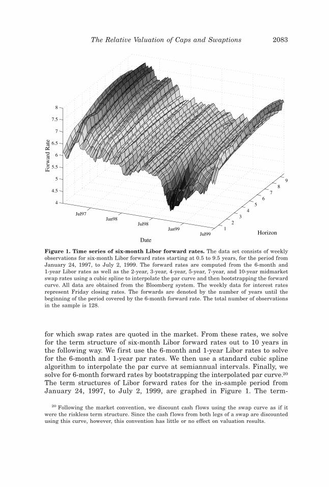
The term structures of Libor forward rates for the in-sample period fromJanuary 24, 1997, to July 2, 1999, are graphed in Figure 1. The term-

20 Following the market convention, we discount cash f lows using the swap curve as if itwere the riskless term structure. Since the cash f lows from both legs of a swap are discountedusing this curve, however, this convention has little or no effect on valuation results.

Figure 1. Time series of six-month Libor forward rates. The data set consists of weeklyobservations for six-month Libor forward rates starting at 0.5 to 9.5 years, for the period fromJanuary 24, 1997, to July 2, 1999. The forward rates are computed from the 6-month and1-year Libor rates as well as the 2-year, 3-year, 4-year, 5-year, 7-year, and 10-year midmarketswap rates using a cubic spline to interpolate the par curve and then bootstrapping the forwardcurve. All data are obtained from the Bloomberg system. The weekly data for interest ratesrepresent Friday closing rates. The forwards are denoted by the number of years until thebeginning of the period covered by the 6-month forward rate. The total number of observationsin the sample is 128.


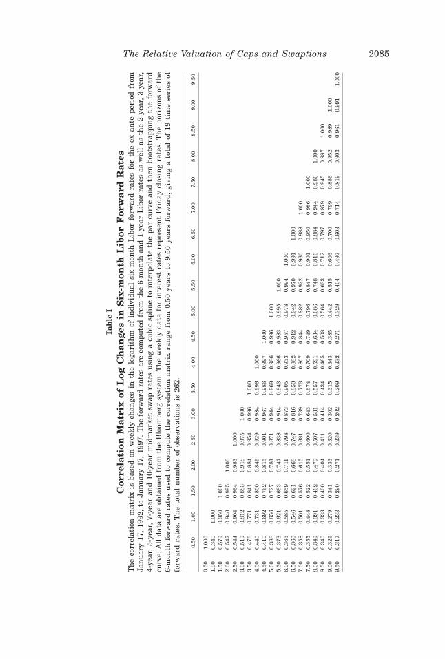
structure data for the 5-year ex ante period from January 17, 1992, to Jan-uary 17, 1997, is used to estimate the historical correlation matrix H fromwhich the eigenvectors used in solving for the implied covariance matricesare determined. This ex ante correlation matrix is shown in Table I; all ofthe in-sample results are based on this ex ante correlation matrix. Note thatthe correlations are generally smooth monotonically decreasing functionsof the distance between forward rates. One interesting exception is the cor-relation between the first and second forwards; the first two forwards dis-play a significant amount of independent variation, hinting at money-market factors not present in longer-term forward rates.

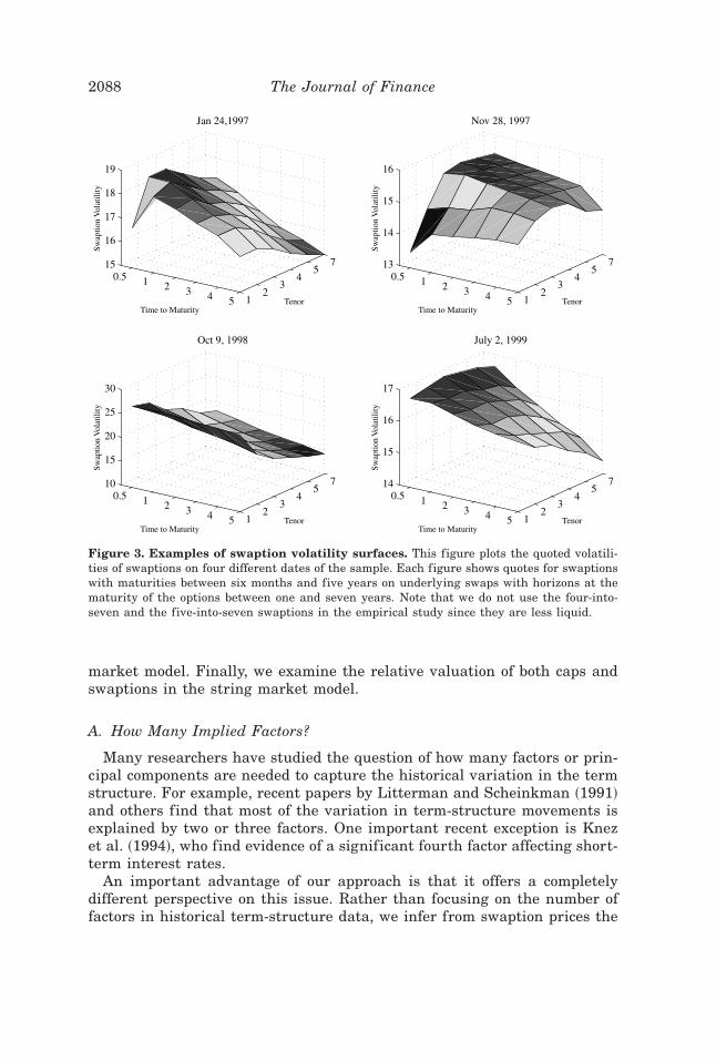
The swaption data consists of weekly midmarket implied volatilities for 34at-the-money-forward European swaptions for the in-sample period from Jan-uary 24, 1997, to July 2, 1999. These 34 swaptions represent all of the stan-dard quoted t by T European swaption structures where the final maturitydate of the underlying swap is less than or equal to 10 years, T � 10. Asdescribed earlier, the market convention is to quote swaption prices in termsof their implied volatility relative to the Black ~1976! model for at-the-money-forward European swaptions given in equation ~7!; the market prices of theseswaptions are given by substituting the implied volatilities into the Blackmodel. Table II provides summary statistics for the implied volatilities. Fig-ure 2 graphs the implied volatilities over time; Figure 3 shows a number ofexamples of the shape of the swaption implied volatility surface at differentpoints in time during the sample period.

Observe that there is a significant spike in these implied volatilities dur-ing the fall of 1998. This spike coincides with the hedge-fund crisis precip-itated by the announcement in early September 1998 of massive tradinglosses by Long Term Capital Management ~LTCM!. The sudden threat to thesolvency of LTCM, which had been widely viewed as a premier client bymany Wall Street firms, created a near panic in the financial markets. Inthe subsequent weeks, a number of other highly leveraged hedge funds alsoannounced that they had experienced large trading losses on positions sim-ilar to those held by LTCM. Examples of these funds included ConvergenceCapital Management, Ellington Capital Management, D. E. Shaw & Co.,and MKP Capital Management. In an effort to stabilize the market, theFederal Reserve Bank of New York persuaded a consortium of 16 investmentand commercial banks to inject $3.6 billion into LTCM in exchange for vir-tually all of the remaining equity in the fund. The prompt action by theFederal Reserve, announced to the markets on September 24, 1998, allowedLTCM to avoid insolvency and reduced the pressure on the fund to unwindtrading positions at illiquid fire-sale prices, which would have exacerbatedthe problems at other hedge funds to which the consortium members hadconsiderable risk exposure.

The interest-rate cap data consists of weekly midmarket implied volatili-ties for 2-year, 3-year, 4-year, 5-year, 7-year, and 10-year caps for the sameperiod as for the swaptions data, January 24, 1997, to July 2, 1999. Bymarket convention, the strike price of a T-year cap is simply the T-year


Ta

ble

I

Cor

rela

tion

Mat

rix

ofL

ogC

han

ges

inS

ix-m

onth

Lib

orF

orw

ard

Rat

esT

he

corr

elat

ion

mat

rix

isba

sed

onw

eekl

ych

ange

sin

the

loga

rith

mof

indi

vidu

alsi

x-m

onth

Lib

orfo

rwar

dra

tes

for

the

exan

tepe

riod

from

Jan

uar

y17

,19

92,

toJa

nu

ary

17,

1997

.T

he

forw

ard

rate

sar

eco

mpu

ted

from

the

6-m

onth

and

1-ye

arL

ibor

rate

sas

wel

las

the

2-ye

ar,

3-ye

ar,

4-ye

ar,

5-ye

ar,

7-ye

aran

d10

-yea

rm

idm

arke

tsw

apra

tes

usi

ng

acu

bic

spli

ne

toin

terp

olat

eth

epa

rcu

rve

and

then

boot

stra

ppin

gth

efo

rwar

dcu

rve.

All

data

are

obta

ined

from

the

Blo

ombe

rgsy

stem

.T

he

wee

kly

data

for

inte

rest

rate

sre

pres

ent

Fri

day

clos

ing

rate

s.T

he

hor

izon

sof

the

6-m

onth

forw

ard

rate

su

sed

toco

mpu

teth

eco

rrel

atio

nm

atri

xra

nge

from

0.50

year

sto

9.50

year

sfo

rwar

d,gi

vin

ga

tota

lof

19ti

me

seri

esof

forw

ard

rate

s.T

he

tota

ln

um

ber

ofob

serv

atio

ns

is26

2.

0.50

1.00

1.50

2.00

2.50

3.00

3.50

4.00

4.50

5.00

5.50

6.00

6.50

7.00

7.50

8.00

8.50

9.00

9.50

0.50

1.00

01.

000.

340

1.00

01.

500.

579

0.95

01.

000

2.00

0.54

70.

946

0.99

51.

000

2.50

0.54

40.

904

0.96

40.

983

1.00

03.

000.

519

0.81

20.

883

0.91

80.

975

1.00

03.

500.

476

0.77

10.

841

0.88

40.

954

0.99

61.

000

4.00

0.44

00.

731

0.80

00.

849

0.92

90.

984

0.99

61.

000

4.50

0.41

00.

692

0.76

20.

815

0.90

10.

967

0.98

60.

997

1.00

05.

000.

388

0.65

60.

727

0.78

10.

871

0.94

40.

969

0.98

60.

996

1.00

05.

500.

373

0.62

10.

693

0.74

70.

838

0.91

40.

943

0.96

60.

983

0.99

51.

000

6.00

0.36

50.

585

0.65

90.

711

0.79

80.

873

0.90

50.

933

0.95

70.

978

0.99

41.

000

6.50

0.36

00.

546

0.62

10.

668

0.74

70.

816

0.85

00.

882

0.91

20.

942

0.97

00.

991

1.00

07.

000.

358

0.50

10.

576

0.61

50.

681

0.73

90.

773

0.80

70.

844

0.88

20.

922

0.96

00.

988

1.00

07.

500.

355

0.44

80.

522

0.55

10.

600

0.64

30.

674

0.70

90.

749

0.79

60.

847

0.90

10.

950

0.98

61.

000

8.00

0.34

90.

391

0.46

20.

479

0.50

70.

531

0.55

70.

591

0.63

40.

686

0.74

80.

816

0.88

40.

944

0.98

61.

000

8.50

0.34

00.

333

0.40

00.

404

0.41

10.

414

0.43

40.

465

0.50

80.

564

0.63

30.

712

0.79

70.

879

0.94

50.

987

1.00

09.

000.

329

0.27

90.

341

0.33

30.

320

0.30

20.

315

0.34

30.

385

0.44

20.

515

0.60

30.

700

0.79

90.

886

0.95

20.

989

1.00

09.

500.

317

0.23

30.

290

0.27

10.

239

0.20

20.

209

0.23

20.

271

0.32

90.

404

0.49

70.

603

0.71

40.

819

0.90

30.

961

0.99

11.

000


swap rate. To parallel the features of swaptions and to simplify the analysis,we assume that caps are on the 6-month Libor rate rather than the 3-monthrate.21 The market prices of caps are then given by substituting the impliedvolatility into the Black model ~1976! given in equation ~1!, where T � t �102. Table III presents summary statistics for the market cap volatilities

Table II

Summary Statistics for OTC Market At-the-Money-ForwardEuropean Swaption Volatilities

The data set consists of 128 weekly observations from January 24, 1997, to July 2, 1999, ofmidmarket implied Black-model volatilities for the indicated N into M at-the-money-forwardEuropean swaption structure, where N denotes years until option expiration and M denotes thelength of the underlying swap in years.

N M MeanStandardDeviation Minimum Median Maximum

SerialCorrelation

0.50 1.00 14.60 3.37 9.70 13.50 27.00 0.9261.00 1.00 16.10 2.98 11.80 15.35 11.80 0.9452.00 1.00 16.66 2.27 13.10 16.20 13.10 0.9403.00 1.00 16.42 1.99 13.00 16.10 13.00 0.9324.00 1.00 16.08 1.72 13.00 15.95 13.00 0.9415.00 1.00 15.73 1.48 12.90 15.70 12.90 0.9330.50 2.00 15.35 3.10 10.40 14.45 10.40 0.9191.00 2.00 16.08 2.59 12.20 15.50 12.20 0.9432.00 2.00 16.31 2.05 13.00 16.00 13.00 0.9363.00 2.00 16.02 1.74 12.90 15.85 12.90 0.9394.00 2.00 15.70 1.51 12.80 15.70 12.80 0.9315.00 2.00 15.38 1.34 12.70 15.50 12.70 0.9250.50 3.00 15.34 2.93 10.60 14.65 10.60 0.9131.00 3.00 15.89 2.35 12.20 15.30 12.20 0.9372.00 3.00 16.00 1.84 12.90 15.70 12.90 0.9333.00 3.00 15.72 1.57 12.80 15.65 12.80 0.9274.00 3.00 15.42 1.37 12.70 15.50 12.70 0.9295.00 3.00 15.09 1.23 12.60 15.20 12.60 0.9200.50 4.00 15.32 2.73 10.80 14.70 10.80 0.9061.00 4.00 15.67 2.14 12.10 15.30 12.10 0.9302.00 4.00 15.72 1.64 12.80 15.65 12.80 0.9333.00 4.00 15.45 1.42 12.70 15.50 12.70 0.9304.00 4.00 15.14 1.27 12.60 15.20 12.60 0.9185.00 4.00 14.80 1.14 12.50 15.00 12.50 0.9170.50 5.00 15.30 2.57 11.00 14.70 11.00 0.8971.00 5.00 15.42 1.93 12.00 15.20 12.00 0.9262.00 5.00 15.45 1.49 12.70 15.40 12.70 0.9243.00 5.00 15.18 1.32 12.60 15.25 12.60 0.9324.00 5.00 14.85 1.18 12.50 15.00 12.50 0.9195.00 5.00 14.48 1.04 12.50 14.70 12.50 0.9090.50 7.00 15.09 2.41 11.00 14.60 11.00 0.8871.00 7.00 15.10 1.71 12.00 15.00 12.00 0.9142.00 7.00 15.03 1.38 12.40 15.05 12.40 0.9213.00 7.00 14.77 1.24 12.30 14.90 12.30 0.913


during the sample period. The implied volatilities display a time-series pat-tern similar to those observed for swaptions. Figure 4 also graphs the timeseries of cap volatilities.

IV. The Empirical Results

In this section, we report the empirical results from the study. First, weexamine how many implied factors are required to explain the market pricesof swaptions. We then study the relative valuation of swaptions in the string

21 This assumption is relatively innocuous. We have spoken with several caps dealers whoindicated that the implied volatilities for caps on six-month Libor would typically be equal to oran eighth to a quarter below the implied volatility for a cap on three-month Libor. Diagnostictests presented later in the paper indicate that this assumption has virtually no effect on theempirical results.

Figure 2. Time series of swaption volatilities. The data set consists of 128 weekly obser-vations from January 24, 1997, to July 2, 1999, of midmarket implied Black-model volatilitiesfor the indicated N into M at-the-money-forward European swaption structure, where N de-notes years until option expiration ~time to maturity! and M denotes the length of the under-lying swap in years ~the tenor!. The subplots show, for each tenor, the implied volatilities ofoptions with different times to maturity.


market model. Finally, we examine the relative valuation of both caps andswaptions in the string market model.

A. How Many Implied Factors?

Many researchers have studied the question of how many factors or prin-cipal components are needed to capture the historical variation in the termstructure. For example, recent papers by Litterman and Scheinkman ~1991!and others find that most of the variation in term-structure movements isexplained by two or three factors. One important recent exception is Knezet al. ~1994!, who find evidence of a significant fourth factor affecting short-term interest rates.

An important advantage of our approach is that it offers a completelydifferent perspective on this issue. Rather than focusing on the number offactors in historical term-structure data, we infer from swaption prices the

Figure 3. Examples of swaption volatility surfaces. This figure plots the quoted volatili-ties of swaptions on four different dates of the sample. Each figure shows quotes for swaptionswith maturities between six months and five years on underlying swaps with horizons at thematurity of the options between one and seven years. Note that we do not use the four-into-seven and the five-into-seven swaptions in the empirical study since they are less liquid.


actual number of factors that market participants view as important inf lu-ences on the term structure. Since the implied factor structure is forwardlooking, the number of implied factors need not be the same as those ob-tained historically. Intuitively, this approach is analogous to the familiartechnique of solving for the implied volatility in option prices; implied vol-atilities typically do not equal estimates of volatility based on historical data,and often provide more accurate forecasts of future volatility.22

We estimate the implied number of factors using an incremental likeli-hood ratio test based on all 128 weekly observations for each of the 34 Eu-ropean swaptions in the data set. Recall that when all but the first Neigenvalues in the diagonal matrix are equal to zero, the implied covari-ance matrix is of rank N, or equivalently, the implied covariance matrix isgenerated by N factors. For a given value of N, and for the ith week i �1,2, . . . ,128, we use the procedure described in Section III.B to solve for theN-implied eigenvalues that minimize the sum of squared percentage swap-tion pricing errors, where the percentage errors are defined as the differ-ences between the simulated and market values of each swaption, expressedas a percentage of the market value of the swaption. Note that these pricingerrors arise because we are trying to fit 34 swaption prices with only N � 34parameters. Thus, these errors have an interpretation very similar to that ofthe residuals from a nonlinear least squares regression. We repeat the pro-cess of solving for the N eigenvalues that minimize the sum of squared per-

22 We note that other researchers have also used the approach of backing out factors fromasset prices such as bonds. Important recent examples of this approach include Longstaff andSchwartz ~1992!, Chen and Scott ~1993!, Pearson and Sun ~1994!, Duffie and Singleton ~1997!,de Jong and Santa-Clara ~1999!, Dai and Singleton ~2000!, Duffee ~2000!, and many others. Ourapproach differs in that we use the information in swaption prices to address the question ofthe number of factors. Intuitively, it is clear that since swaptions have nonlinear payoffs, theirprices may contain more information about market estimates of the conditional volatility offactors than can be recovered from bond prices alone.

Table III

Summary Statistics for OTC Market LiborInterest-rate Cap Volatilities

The data set consists of 128 weekly observations from January 24, 1997, to July 2, 1999, ofmidmarket implied Black-model volatilities for the indicated cap maturities. All data are ob-tained from Bloomberg.

CapMaturity Mean

StandardDeviation Minimum Median Maximum

SerialCorrelation

2 Year 15.34 3.19 10.60 14.25 28.00 0.9453 Year 16.43 2.75 12.10 15.60 25.20 0.9404 Year 16.75 2.41 12.50 16.10 23.50 0.9325 Year 16.84 2.21 12.90 16.30 22.75 0.9417 Year 16.46 1.86 12.75 16.15 20.87 0.933

10 Year 15.97 1.55 12.60 15.90 19.75 0.919


centage pricing errors for each of the 128 weeks in the sample period. Addingthe sum of squared errors over all 128 weeks gives the total sum of squarederrors. We then repeat this entire procedure for the case of N � 1 eigen-values, where the same seed for the random number generator is used for allvalues of N to insure comparability in the results. Under the null hypothesisof equality, 128 � 34 � 4,352 times the difference between the logarithms ofthe sum of squared errors for N and N � 1 factors is asymptotically distrib-uted as a chi-square variate with 128 degrees of freedom.

Table IV reports the results from the incremental pairwise comparisons asN ranges from one to seven. As shown, the pairwise comparisons are statis-tically significant for two versus one, three versus two, and four versus threefactors, and are insignificant for all of the other comparisons. These resultsimply that there are four significant factors underlying the covariance ma-trix of forwards used by the market in the pricing of European swaptions.These results contrast with the earlier empirical work mentioned above, whichfinds only two to three factors in historical term-structure movements. It isimportant to mention, however, that most of these earlier studies focus onTreasury bonds whereas our results apply to the swap curve. Thus, it is

Figure 4. Time series of cap volatilities. The data set consists of 128 weekly observationsfrom January 24, 1997, to July 2, 1999, of midmarket implied Black-model volatilities for theindicated cap maturities.


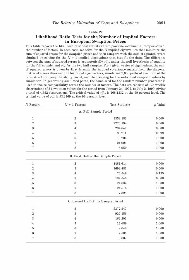
Table IV

Likelihood Ratio Tests for the Number of Implied Factorsin European Swaption Prices

This table reports the likelihood ratio test statistics from pairwise incremental comparisons ofthe number of factors. In each case, we solve for the N-implied eigenvalues that minimize thesum of squared errors for the swaption prices and then compare with the sum of squared errorsobtained by solving for the N � 1 implied eigenvalues that best fit the data. The differencebetween the sum of squared errors is asymptotically x128

2 under the null hypothesis of equalityfor the full sample, and x64

2 for the two half samples. For a given vector of eigenvalues, the sumof squared errors is given by first forming the implied covariance matrix from the diagonalmatrix of eigenvalues and the historical eigenvectors, simulating 2,000 paths of evolution of theterm structure using the string model, and then solving for the individual swaption values bysimulation. In generating simulated paths, the same seed for the random number generator isused to insure comparability across the number of factors. The data set consists of 128 weeklyobservations of 34 swaption values for the period from January 24, 1997, to July 2, 1999, givinga total of 4,352 observations. The critical value of x128

2 is 168.1332 at the 99 percent level. Thecritical value of x64

2 is 93.2169 at the 99 percent level.

N Factors N � 1 Factors Test Statistic p-Value

A. Full Sample Period

1 2 3352.183 0.000

2 3 2220.194 0.000

3 4 284.847 0.000

4 5 86.211 0.998

5 6 13.204 1.000

6 7 21.991 1.000

7 8 3.959 1.000

B. First Half of the Sample Period

1 2 4481.614 0.000

2 3 1699.481 0.000

3 4 76.549 0.135

4 5 137.540 0.000

5 6 24.084 1.000

6 7 24.516 1.000

7 8 7.324 1.000

C. Second Half of the Sample Period

1 2 2377.247 0.000

2 3 922.156 0.000

3 4 162.201 0.000

4 5 17.689 1.000

5 6 2.048 1.000

6 7 7.505 1.000

7 8 0.607 1.000


possible that the existence of a credit factor inf luencing swap rates but notTreasury rates could reconcile our results with those obtained by earlierresearchers. Because of these results, all of our subsequent analysis is basedon implied covariance matrices generated by four eigenvalues, resulting infour-factor or rank-four implied covariance matrices.

As a robustness check, we also conduct the incremental likelihood ratiotests using only the first half of the sample period ~64 weeks! and also usingonly the second half of the sample period ~64 weeks!. Since the hedge-fundcrisis of fall 1998 occurred entirely during the second half of the sampleperiod, this diagnostic addresses whether the results about the number offactors are specific to this volatile period. As shown, however, the subperiodresults are similar to those for the entire period. In both the first and secondsubperiods, the likelihood ratio tests find evidence of four statistically sig-nificant factors. Thus, the results about the number of factors are not arti-facts of the hedge-fund crisis of fall 1998.23

To provide some insight into the four implied factors that market partici-pants view as driving the term structure, Figure 5 graphs the first foureigenvectors, which define the weights of the first four factors, from thehistorical correlation matrix in Table I. As illustrated, these factors closelyresemble those found in earlier papers. The first factor essentially generatesparallel shifts in the term structure. The second factor generates shifts inthe slope of the term structure. The third factor is a curvature factor thatgenerates movements in the term structure where short-term and long-termrates move in opposite directions from the midterm rates. Finally, the fourthfactor primarily affects the shape of the very short end of the term structure,possibly ref lecting the inf luence of the Federal Reserve or other monetaryauthorities. Thus, this fourth factor has an interpretation very similar to thefourth factor found by Knez et al. ~1994! in their study of short-term rates.

Since the eigenvectors used in solving for the implied covariance matrixhave the interpretation of term-structure factors, the fitted eigenvalues canbe viewed as the implied variances of the factors. To illustrate this, Figure 6graphs the time series of fitted values for each of the four eigenvalues usedto define the implied covariance matrix. The first eigenvalue shows the rel-ative volatility over time of the parallel shift factor. The volatility of thisfactor was very stable during much of 1997, decreased somewhat during theearly part of 1998, and then increased significantly during the fall of 1998when the financial stability of a number of highly visible hedge funds wasthreatened by severe trading losses. The volatility of the term-structure slopefactor decreased significantly during 1997, and was quite low during most of

23 It is interesting to note that the four significant factors during the first half of the sampleare the first, second, third, and fifth, while the four significant factors during the entire sampleperiod and during the second half of the sample period are the first, second, third, and fourth.Thus, one could argue that as many as five factors could occasionally be needed to describeswaption prices. We take the more parsimonious view that there are only four significant fac-tors based on the results for the full sample period.


1998. In the fall of 1998, however, the volatility of this factor suddenly in-creased by a factor of nearly 10, but then quickly returned to levels nearthose at the beginning of the sample period. The volatility of the curvaturefactor shows a pattern similar to that of the slope factor; the volatility de-creases significantly during 1997, is generally low during most of 1998, andthen spikes dramatically during the fall of 1998. The behavior of the vola-tility of the short-term or fourth factor suggests one possible way of recon-ciling these results with the historical evidence on the number of factors.The implied volatility of this fourth factor is often quite small and can ac-tually be zero. During periods of market stress such as the fall of 1998,

Figure 5. Eigenvector weights. The four subplots show the weights of the first four eigen-vectors of the historical correlation matrix. The correlation matrix is based on weekly changesin the logarithm of individual six-month Libor forward rates for the ex ante period from Jan-uary 17, 1992, to January 17, 1997. The forward rates are computed from the six-month andone-year Libor rates as well as the two-year, three-year, four-year, five-year, seven-year and10-year midmarket swap rates using a cubic spline to interpolate the par curve and then boot-strapping the forward curve. The weekly data for interest rates represents Friday closing rates.The horizons of the six-month forward rates used to compute the correlation matrix range from0.50 years to 9.50 years forward, giving a total of 19 time series of forward rates. The totalnumber of observations is 262.


however, the volatility of this factor can suddenly increase and become amajor source of term-structure movements. Thus, the time-series pattern ofthe volatility of the fourth factor suggests that this may be more of an event-related factor that only becomes important in periods of extreme marketstress. Since historical analysis of the number of factors is typically based onunconditional tests, factors that have time-varying volatilities that are usu-ally small or zero may not show up in these types of standard tests. Despitethis, these factors could represent a serious source of conditional volatilityrisk to market participants who would appropriately incorporate their ef-fects into the market prices of swaptions. Recent papers by Hull and White~1999! and Jagannathan and Sun ~1999! independently confirm that threefactors are not sufficient to fully capture the pricing of interest rate capsand swaptions. Peterson, Stapleton, and Subrahmanyam ~2000! find thatgoing from one to two term-structure factors has a significant effect on thevaluation of swaptions.

Figure 6. Time series of eigenvalues. The four subplots show the eigenvalues computedfrom the 128 weekly implied correlation matrices from January 24, 1997, to July 2, 1999,obtained by fitting the model to the swaption data, keeping fixed the eigenvectors of the his-torical correlation matrix.


B. The Implied Correlation Matrix

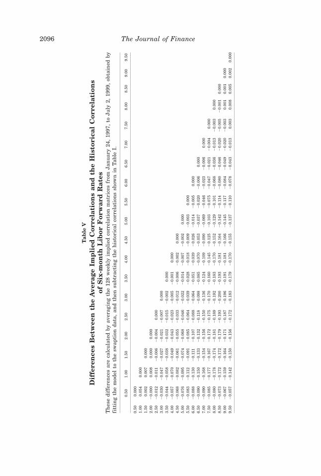
As discussed, the implied eigenvalues uniquely determine the impliedcovariance matrix. In this sense, our approach is simply the matrix ver-sion of the familiar technique of inverting option prices to solve forthe implied volatility of the underlying asset. One natural question thatarises is how closely the implied correlation matrix matches the histori-cal correlation matrix. To compare the two, we do the following. Basedon the results of the likelihood ratio tests in the previous section, weset N � 4 and use the corresponding four implied eigenvalues for eachweek to define a diagonal matrix for each week. This diagonal matrix has the four implied eigenvalues as the first four elements along thediagonal, and zeros as the remaining diagonal elements. From and thehistorical matrix of eigenvectors U, the implied covariance matrix for thatweek is defined by � � UU '. Standardizing the covariance matrix givesthe implied correlation matrix for that week. We repeat this process for all128 weeks in the sample, resulting in a series of 128 implied correlationmatrices.

To obtain summary measures of implied correlations, we then compute thematrix of average implied correlations by simply taking the time series av-erage of each element in the implied correlation matrix over all 128 weeks.We then take the difference between the matrix of average implied correla-tions and the historical correlation matrix in Table I and report these dif-ferences in Table V. To provide some sense of the time-series variation inthese differences, Table VI reports the matrix of standard deviations of theimplied correlations.

As shown in Table V, there are clearly systematic differences between thehistorical and implied correlations. The differences along the main diagonalare all zero, of course, since the main diagonals of both the implied andhistorical correlation matrices consist of ones. As we move away from themain diagonal, however, the differences are almost all negative, which meansthat the implied correlations tend to be lower than the historical correla-tions. Most of the differences are on the order of 0.05 to 0.10, but a few areas large as 0.20. The largest differences are typically for the correlation oftwo-to-three-year forwards with seven-to-nine-year forwards. The only no-table positive difference is for the correlation between the first and secondforwards.

Table VI shows that there is a fair amount of time-series variation in theimplied correlations, indicating that the implied correlation matrix is notconstant over time. In general, however, the standard deviations do notappear to be excessively variable; most of the standard deviations rangefrom 0.05 to 0.20. The largest standard deviation is for the correlationbetween the first and second forwards. Intuitively, however, it is thiscorrelation that is likely to be the hardest to estimate since it only affectsone of the swaptions; all of the other correlations affect multiple swaptionvalues.


Ta

ble

V

Dif

fere

nce

sB

etw

een

the

Ave

rage

Imp

lied

Cor

rela

tion

san

dth

eH

isto

rica

lC

orre

lati

ons

ofS

ix-m

onth

Lib

orF

orw

ard

Rat

esT

hes

edi

ffer

ence

sar

eca

lcu

late

dby

aver

agin

gth

e12

8w

eekl

yim

plie

dco

rrel

atio

nm

atri

ces

from

Jan

uar

y24

,19

97,

toJu

ly2,

1999

,ob

tain

edby

fitt

ing

the

mod

elto

the

swap

tion

data

,an

dth

ensu

btra

ctin

gth

eh

isto

rica

lco

rrel

atio

ns

show

nin

Tab

leI.

0.50

1.00

1.50

2.00

2.50

3.00

3.50

4.00

4.50

5.00

5.50

6.00

6.50

7.00

7.50

8.00

8.50

9.00

9.50

0.50

0.00

01.

000.

054

0.00

01.

500.

002

0.00

70.

000

2.00

�0.

000

0.00

80.

000

0.00

02.

50�

0.01

2�

0.01

1�

0.00

6�

0.00

40.

000

3.00

�0.

030

�0.

047

�0.

027

�0.

021

�0.

007

0.00

03.

50�

0.04

4�

0.05

8�

0.03

8�

0.03

2�

0.01

5�

0.00

20.

000

4.00

�0.

057

�0.

070

�0.

049

�0.

043

�0.

023

�0.

005

�0.

001

0.00

04.

50�

0.06

8�

0.08

2�

0.06

1�

0.05

5�

0.03

3�

0.01

2�

0.00

6�

0.00

20.

000

5.00

�0.

076

�0.

095

�0.

074

�0.

068

�0.

046

�0.

022

�0.

014

�0.

007

�0.

002

0.00

05.

50�

0.08

3�

0.11

2�

0.09

1�

0.08

5�

0.06

4�

0.03

9�

0.02

8�

0.01

8�

0.00

9�

0.00

30.

000

6.00

�0.

088

�0.

130

�0.

111

�0.

107

�0.

088

�0.

064

�0.

051

�0.

039

�0.

026

�0.

014

�0.

005

0.00

06.

50�

0.09

0�

0.15

0�

0.13

3�

0.13

2�

0.11

8�

0.09

8�

0.08

5�

0.07

0�

0.05

3�

0.03

7�

0.02

0�

0.00

60.

000

7.00

�0.

090

�0.

168

�0.

154

�0.

156

�0.

150

�0.

136

�0.

124

�0.

109

�0.

090

�0.

069

�0.

046

�0.

023

�0.

006

0.00

07.

50�

0.08

5�

0.17

7�

0.16

7�

0.17

2�

0.17

5�

0.17

0�

0.16

0�

0.14

5�

0.12

5�

0.10

3�

0.07

5�

0.04

7�

0.02

1�

0.00

40.

000

8.00

�0.

080

�0.

178

�0.

174

�0.

181

�0.

189

�0.

192

�0.

183

�0.

170

�0.

152

�0.

129

�0.

101

�0.

068

�0.

036

�0.

013

�0.

003

0.00

08.

50�

0.07

3�

0.17

2�

0.17

2�

0.17

9�

0.19

3�

0.20

0�

0.19

3�

0.18

1�

0.16

4�

0.14

2�

0.11

4�

0.08

0�

0.04

6�

0.02

0�

0.00

5�

0.00

10.

000

9.00

�0.

067

�0.

159

�0.

164

�0.

171

�0.

187

�0.

196

�0.

191

�0.

181

�0.

166

�0.

145

�0.

117

�0.

084

�0.

049

�0.

020

�0.

003

0.00

10.

001

0.00

09.

50�

0.05

7�

0.14

2�

0.15

0�

0.15

6�

0.17

2�

0.18

3�

0.17

9�

0.17

0�

0.15

5�

0.13

7�

0.11

0�

0.07

8�

0.04

3�

0.01

30.

003

0.00

80.

005

0.00

20.

000


Ta

ble

VI

Sta

nd

ard

Dev

iati

ons

ofth

eIm

pli

edC

orre

lati

ons

ofS

ix-m

onth

Lib

orF

orw

ard

Rat

esT

his

tabl

ere

port

sth

est

anda

rdde

viat

ion

sof

the

indi

vidu

alel

emen

tsof

the

128

wee

kly

impl

ied

corr

elat

ion

mat

rice

sfr

omJa

nu

ary

24,

1997

,to

July

2,19

99,

obta

ined

byfi

ttin

gth

em

odel

toth

esw

apti

onda

ta,

and

then

subt

ract

ing

the

his

tori

cal

corr

elat

ion

ssh

own

inT

able

I.

0.50

1.00

1.50

2.00

2.50

3.00

3.50

4.00

4.50

5.00

5.50

6.00

6.50

7.00

7.50

8.00

8.50

9.00

9.50

0.50

0.00

01.

000.

602

0.00

01.

500.

404

0.05

40.

000

2.00

0.38

00.

056

0.00

20.

000

2.50

0.25

10.

097

0.01

40.

007

0.00

03.

000.

116

0.15

50.

047

0.03

70.

013

0.00

03.

500.

120

0.14

60.

072

0.05

40.

026

0.00

40.

000

4.00

0.13

90.

140

0.09

90.

076

0.04

50.

013

0.00

30.

000

4.50

0.15

90.

139

0.12

40.

099

0.06

50.

025

0.01

00.

002

0.00

05.

000.

174

0.14

30.

146

0.12

10.

085

0.04

10.

022

0.01

00.

003

0.00

05.

500.

183

0.15

10.

166

0.14

20.

107

0.06

10.

039

0.02

40.

012

0.00

40.

000

6.00

0.18

10.

161

0.18

30.

162

0.13

20.

088

0.06

60.

048

0.03

10.

017

0.00

50.

000

6.50

0.16

90.

174

0.19

60.

181

0.16

00.

123

0.10

30.

083

0.06

40.

044

0.02

40.

007

0.00

07.

000.

151

0.18

20.

201

0.19

50.

185

0.16

10.

144

0.12

50.

104

0.08

10.

055

0.02

80.

007

0.00

07.

500.

139

0.18

30.

197

0.19

90.

200

0.18

90.

177

0.16

10.

142

0.11

80.

089

0.05

60.

026

0.00

60.

000

8.00

0.14

40.

176

0.18

50.

193

0.20

40.

203

0.19

60.

184

0.16

80.

146

0.11

70.

082

0.04

70.

019

0.00

40.

000

8.50

0.16

30.

165

0.16

90.

180

0.19

60.

203

0.20

00.

193

0.18

00.

161

0.13

40.

101

0.06

40.

032

0.01

20.

003

0.00

09.

000.

188

0.15

20.

151

0.16

30.

181

0.19

40.

194

0.19

00.

181

0.16

60.

142

0.11

10.

075

0.04

30.

021

0.00

80.

002

0.00

09.

500.

214

0.14

00.

135

0.14

60.

165

0.18

00.

184

0.18

30.

177

0.16

50.

145

0.11

70.

083

0.05

30.

030

0.01

60.

006

0.00

10.

000


C. The Relative Valuation of Swaptions

The structure of the string market model imposes a number of constraintson the dynamic evolution of the term structure. Because of this, it is impor-tant to examine how well the model is able to describe the underlying struc-ture of market swaption prices. Recall that the string market model isattempting to explain the cross section of 34 swaption prices using only fourparameters each period. Thus, the model places a number of overidentifyingrestrictions of swaption prices and the pricing errors from fitting the stringmarket model provide insights into how well these overidentifying restric-tions are satisfied by the data.

To address this issue, Figure 7 graphs the RMSEs for the 34 swaptions inthe sample for each of the 128 weeks in the sample period. Recall that theseRMSEs are computed by first estimating the four eigenvalues that best fitthe market swaption prices for that week, pricing the swaptions by simu-lating paths of the string market model, and then taking the percentage

Figure 7. Time series of swaptions RMSE of four-factor string market model. The graphshows the RMSE of the differences between the fitted model swaptions prices and the marketprices expressed as a percentage of the market prices. The data set consists of 128 weeklyobservations from January 24, 1997, to July 2, 1999, for 34 at-the-money-forward Europeanswaption structures.


differences between the market and model prices. As illustrated, the RMSEsfrom this time-homogeneous string market model are generally very small;the model typically captures the shape of the swaption volatility surfacequite closely. Leaving out the exceptional period in the fall of 1998, the RMSEsare generally between two to three percent. These RMSEs are roughly aboutone-third to one-half of the size of the bid-offer spread.24 The median RMSEis 3.10 percent and the standard deviation of the RMSEs is 2.98 percent.

Although the string market model fits the swaptions market well duringmost of the sample period, the fall of 1998 is clearly a major outlier. Duringthis period, the RMSE spikes up to as high as 16 percent. The period duringwhich the RMSE exceeds five percent begins with the week of September 11,1998. Interestingly, this is just a few days after the well-publicized letterfrom John Meriwether to the investors of LTCM informing them that thefund had lost 52 percent of its capital through the end of August due tomajor trading losses in a number of markets. The RMSEs remain consis-tently above five percent for the 10-week period from September 11, 1998, toNovember 13, 1998, which closely aligns with the period during which mostof the uncertainty about the survival of many of the hedge funds involved inthe crisis was being resolved.

The failure of the string market model to capture the shape of the swap-tions volatility surface during this period raises two possibilities: either theassumption of time-homogeneity is too restrictive, or quoted prices in theswaptions market were inconsistent with the absence of arbitrage. Al-though we cannot completely resolve this classical “joint-hypothesis” prob-lem, we have conducted extensive interviews with many swaptions traderswho experienced this period. These traders generally made two points. First,because of the turbulence in the market, the liquidity in the swaptionsmarket was less than typical, and the quality of the market quotationscollected by Bloomberg could be questioned. Second, there was an almostuniform belief among traders that there were in fact arbitrage opportuni-ties in the markets. Many traders during this period felt that the fear ofa complete market meltdown prevented them from executing trades thatotherwise would have been viewed as highly profitable during ordinarycircumstances.25

Going beyond the overall RMSEs, it is also useful to examine the valua-tion errors for individual swaptions. Although the overall RMSEs are gen-erally small and the fitting procedure requires pricing errors to have a meanclose to zero, individual swaptions could still potentially display systematic

24 Bloomberg reports that the typical bid-offer spread for these swaptions is about one unitof Black-model implied volatility; for a typical implied volatility of 16 percent, a 1 percentvolatility bid-offer spread represents about 6 percent of the value of an at-the-money-forwardswaption.

25 Liu and Longstaff ~2000! demonstrate that rational investors facing realistic margin con-straints may actually choose to underinvest in arbitrages, or avoid investing in an arbitragealtogether, because of the risk that the arbitrage opportunity may widen further before it ul-timately converges.


patterns of mispricing. To investigate this possibility, Table VII reports sum-mary statistics for the pricing errors of individual swaption structures.

As shown, there are some clear patterns in the valuation errors. First,many of the valuation errors are highly serially correlated, implying thatdeviations between the model and market prices are persistent. Generally,

Table VII

Summary Statistics for Percentage Swaption Valuation ErrorsThe summary statistics reported are for the differences between the fitted model price and themarket price expressed as a percentage of the market price. The data set consists of 128 weeklyobservations from January 24, 1997, to July 2, 1999, for the indicated N into M at-the-money-forward European swaption structures, where N denotes years until option expiration and Mdenotes the tenor or length of the underlying swap in years. The t-statistic for the mean and thestandard deviation reported are adjusted for first-order serial correlation. The overall statisticsare simple averages of the corresponding columns with the exception of the overall minimum,median, and maximum, which are computed from all observations.

N M Meant-Stat.Mean


SerialCorrelation

0.50 1.00 �2.456 �1.26 1.954 �19.623 �1.032 6.406 0.9061.00 1.00 �1.123 �1.45 0.775 �12.922 �1.560 5.423 0.7272.00 1.00 �2.124 �3.57 0.595 �8.583 �2.006 4.383 0.7763.00 1.00 �0.924 �1.30 0.712 �5.146 �1.127 6.726 0.8454.00 1.00 0.501 0.38 1.304 �4.030 �0.177 11.406 0.9175.00 1.00 4.815 1.95 2.475 �1.209 3.470 24.683 0.9350.50 2.00 �1.312 �1.06 1.238 �16.379 �1.033 5.057 0.8531.00 2.00 �0.538 �1.43 0.375 �9.588 �0.273 3.654 0.5752.00 2.00 �1.542 �3.24 0.476 �5.757 �1.577 2.163 0.8093.00 2.00 0.289 0.42 0.685 �3.487 �0.131 9.523 0.8554.00 2.00 1.906 1.35 1.411 �3.041 1.005 14.468 0.9165.00 2.00 5.612 2.51 2.239 �0.995 4.289 24.027 0.9240.50 3.00 �0.030 �0.01 2.332 �22.139 1.786 8.077 0.9071.00 3.00 �1.696 �2.01 0.843 �13.825 �1.294 2.517 0.8712.00 3.00 �1.920 �7.08 0.271 �4.701 �1.907 0.794 0.7453.00 3.00 0.328 0.71 0.461 �6.406 0.112 6.868 0.7934.00 3.00 2.033 1.69 1.201 �2.552 1.323 14.843 0.8955.00 3.00 5.446 2.51 2.168 �0.193 3.976 22.971 0.9340.50 4.00 �0.547 �0.19 2.815 �27.444 1.191 9.925 0.8991.00 4.00 �2.523 �1.68 1.503 �16.314 �2.057 3.209 0.9232.00 4.00 �2.209 �8.81 0.251 �5.382 �2.141 �0.034 0.7633.00 4.00 0.151 0.40 0.373 �2.371 0.014 5.346 0.8044.00 4.00 1.775 1.56 1.137 �2.494 1.124 12.965 0.9125.00 4.00 5.409 2.64 2.045 �0.317 3.839 19.778 0.9390.50 5.00 �1.529 �0.50 3.079 �32.517 0.387 9.693 0.8971.00 5.00 �3.013 �2.62 1.149 �18.546 �2.631 6.900 0.8142.00 5.00 �2.402 �6.42 0.374 �7.244 �2.148 �0.087 0.8173.00 5.00 �0.446 �1.70 0.263 �3.433 �0.396 3.546 0.7434.00 5.00 1.239 1.21 1.026 �1.963 0.383 10.447 0.9155.00 5.00 5.615 2.79 2.013 �0.444 4.609 18.406 0.9440.50 7.00 �3.604 �0.91 3.941 �40.981 �1.438 9.483 0.9091.00 7.00 �5.365 �1.93 2.779 �26.164 �3.978 4.643 0.9372.00 7.00 �5.096 �4.36 1.170 �16.876 �4.053 �2.015 0.9093.00 7.00 �3.382 �15.35 0.220 �7.276 �3.154 �1.265 0.669

Overall �0.255 �1.38 1.343 �40.981 �0.416 24.683 0.852


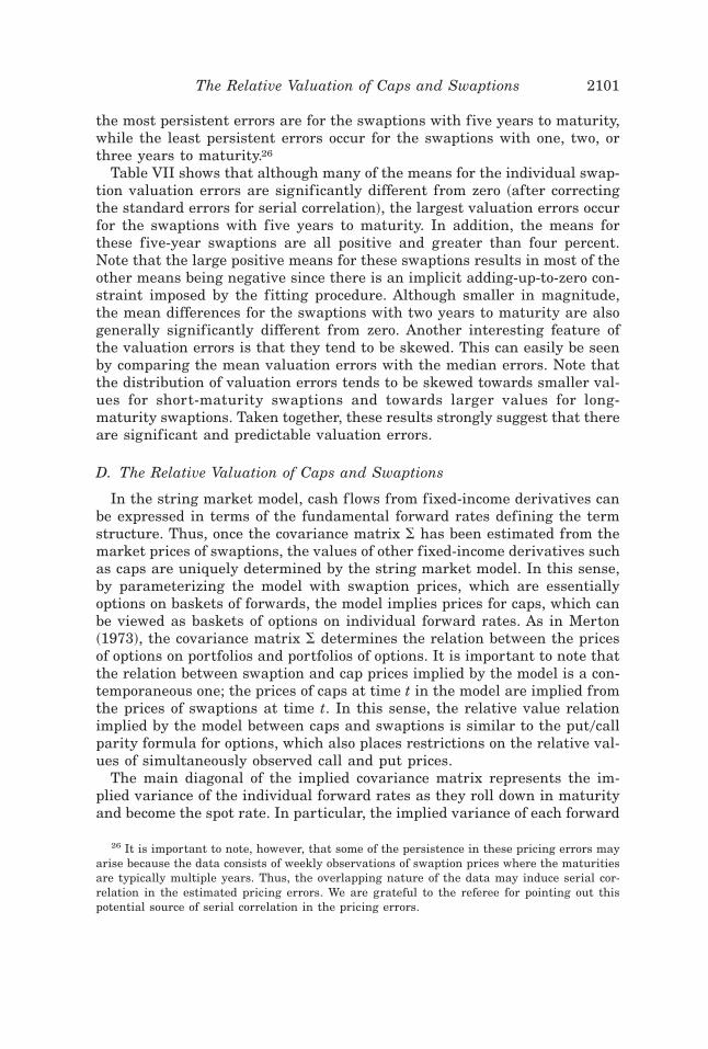
the most persistent errors are for the swaptions with five years to maturity,while the least persistent errors occur for the swaptions with one, two, orthree years to maturity.26

Table VII shows that although many of the means for the individual swap-tion valuation errors are significantly different from zero ~after correctingthe standard errors for serial correlation!, the largest valuation errors occurfor the swaptions with five years to maturity. In addition, the means forthese five-year swaptions are all positive and greater than four percent.Note that the large positive means for these swaptions results in most of theother means being negative since there is an implicit adding-up-to-zero con-straint imposed by the fitting procedure. Although smaller in magnitude,the mean differences for the swaptions with two years to maturity are alsogenerally significantly different from zero. Another interesting feature ofthe valuation errors is that they tend to be skewed. This can easily be seenby comparing the mean valuation errors with the median errors. Note thatthe distribution of valuation errors tends to be skewed towards smaller val-ues for short-maturity swaptions and towards larger values for long-maturity swaptions. Taken together, these results strongly suggest that thereare significant and predictable valuation errors.

D. The Relative Valuation of Caps and Swaptions

In the string market model, cash f lows from fixed-income derivatives canbe expressed in terms of the fundamental forward rates defining the termstructure. Thus, once the covariance matrix � has been estimated from themarket prices of swaptions, the values of other fixed-income derivatives suchas caps are uniquely determined by the string market model. In this sense,by parameterizing the model with swaption prices, which are essentiallyoptions on baskets of forwards, the model implies prices for caps, which canbe viewed as baskets of options on individual forward rates. As in Merton~1973!, the covariance matrix � determines the relation between the pricesof options on portfolios and portfolios of options. It is important to note thatthe relation between swaption and cap prices implied by the model is a con-temporaneous one; the prices of caps at time t in the model are implied fromthe prices of swaptions at time t. In this sense, the relative value relationimplied by the model between caps and swaptions is similar to the put0callparity formula for options, which also places restrictions on the relative val-ues of simultaneously observed call and put prices.

The main diagonal of the implied covariance matrix represents the im-plied variance of the individual forward rates as they roll down in maturityand become the spot rate. In particular, the implied variance of each forward

26 It is important to note, however, that some of the persistence in these pricing errors mayarise because the data consists of weekly observations of swaption prices where the maturitiesare typically multiple years. Thus, the overlapping nature of the data may induce serial cor-relation in the estimated pricing errors. We are grateful to the referee for pointing out thispotential source of serial correlation in the pricing errors.


rate during the last period before it becomes the spot rate is the first ele-ment on the diagonal, the implied variance of each forward rate during thenext-to-last period before it becomes the spot rate is given by the secondelement on the diagonal, and so forth. Since this provides a complete spec-ification of the volatility of all forwards, the main diagonal uniquely deter-mines the values of individual caplets ~conditional on the number ofeigenvalues fitted!, which then determine the values of caps. Thus, once themodel is fitted to the swaptions market, we can directly examine the impli-cations for the valuation of caps. In the absence of arbitrage, the values ofcaps implied by the swaptions market should match the actual market pricesof caps.

To examine the relative valuation of caps and swaptions, we use the maindiagonal of the implied covariance matrix and solve for the implied values of2-year, 3-year, 4-year, 5-year, 7-year, and 10-year at-the-money caps, usingthe Black model given in equation ~1! and the initial term structure to valueindividual caplets. Since the Black model gives a closed-form expression forcaplet prices, we do not need to solve for caps prices by simulation. The useof the Black model for pricing caplets is appropriate here since the lognor-mal dynamics for forward rates given in equation ~8! imply that the Blackmodel holds for individual caplets, since caplets are simple European op-tions on individual forward rates. Note that the variance used in the Blackmodel for valuing a caplet is simply the average variance for the correspond-ing forward rate from the present until the forward becomes the spot rate.Thus, the variance for the caplet maturing in 6 months is the first diagonalelement, the variance for the caplet maturing in 12 months is the average ofthe first and second diagonal elements, and so forth. We repeat this proce-dure for each of the 128 weeks in the sample period and report summarystatistics for the differences between the market and implied prices inTable VIII.

As illustrated, the hypothesis that market cap prices match the valuesimplied by the swaption market is rejected for all of the maturities. Themean percentage pricing errors range from a high of 23.326 for the two-yearcaps down to 5.665 for the five-year caps. The positive means imply that themarket cap prices are undervalued relative to swaptions. Note that thesepercentage pricing errors also tend to display a significant amount of per-sistence as evidenced by their first-order serial correlation coefficients.

A different perspective is obtained by focusing on the median values of thepricing differences. The median pricing errors are all within three percent ofzero, and the overall median is only 0.862, which suggests that the caps andswaptions markets are usually consistent; the significant mean percentagepricing are primarily due to periodic large positive errors, resulting in askewed, somewhat bimodal distribution of errors.

As an additional diagnostic, we also recompute the pricing errors underthe assumption that the Black volatilities for caps on six-month Libor are0.25 volatility points below those for caps on three-month Libor. Recall fromthe earlier discussion that there could be a slight difference in the quoted


volatilities for caps on six-month Libor rather than on three-month Libor.The results, however, are virtually the same as those reported in Table VIII.

As another test of the Merton ~1973! no-arbitrage bounds, we recomputethe percentage pricing differences under the assumption that the correla-tions between all forwards equals one. This is done by fitting only a singleimplied eigenvalue to the market prices of the swaptions; all of the remain-ing eigenvalues are set equal to zero. This specification results in a rank-onecovariance matrix, which in turn, implies perfect correlation among all for-ward rates. Following Merton, it is easily shown that the model price fromthe one-factor model should provide a lower bound for the value of a cap.This is directly an implication of the fact that the value of a portfolio ofoptions should be greater than or equal to the value of an option on a port-folio. Thus, no-arbitrage considerations imply that the percent pricing dif-ferences from the one-factor model should all be positive. Virtually all of thecap prices satisfy this no-arbitrage bound. The mean and median values ofthe percentage pricing differences are now all negative. Of the 128 � 34 �4,352 observations, only 8 or 0.18 percent are positive.

In summary, the evidence suggests that while caps and swaptions almostalways satisfy the strictest no-arbitrage restriction of Merton ~1973!, thevalues of caps and swaptions are frequently inconsistent with each other.This is consistent with Hull and White ~1999! who independently find thata set of cap and swaptions prices for a single day in August 1999 cannot bereconciled within the context of a three-factor model. Similarly, Jagan-nathan and Sun ~1999! find that caps and swaptions appear significantlymispriced in a three-factor Cox, Ingersoll, and Ross ~1985! framework. Ourresults suggest the possibility that whereas buy-and-hold arbitrages maynot be feasible, dynamic trading strategies exploiting inconsistencies in the

Table VIII

Summary Statistics for Percentage Cap Valuation ErrorsThe summary statistics reported are for the percentage difference between the model priceimplied from fitting the string market model to the swaptions market and the market priceexpressed as a percentage of the market price. The data set consists of 128 weekly observationsfrom January 24, 1997, to July 2, 1999, for the indicated maturities. The t-statistic for themean and the standard deviation of the mean reported are adjusted for first-order serial cor-relation. The overall statistics are simple averages of the corresponding columns with the ex-ception of the overall minimum, median, and maximum, which are computed from all observations.

Maturity Meant-Stat.Mean


SerialCorrelation

2.00 23.326 3.50 6.669 �19.484 2.589 113.307 0.6633.00 11.782 2.73 4.319 �11.359 �0.705 63.361 0.6644.00 7.666 2.36 3.245 �9.739 �2.120 47.687 0.6465.00 5.665 2.14 2.644 �9.191 �2.385 38.071 0.6417.00 6.021 2.58 2.332 �8.941 �0.054 32.379 0.685

10.00 7.864 3.57 2.200 �4.592 2.883 32.578 0.734Overall 10.387 2.81 3.568 �19.484 0.862 113.307 0.672


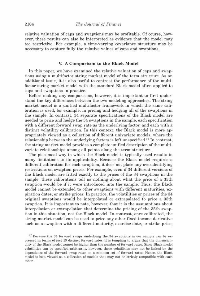
relative valuation of caps and swaptions may be profitable. Of course, how-ever, these results can also be interpreted as evidence that the model maytoo restrictive. For example, a time-varying covariance structure may benecessary to capture fully the relative values of caps and swaptions.

V. A Comparison to the Black Model

In this paper, we have examined the relative valuation of caps and swap-tions using a multifactor string market model of the term structure. As anadditional issue, it is also useful to contrast the performance of the multi-factor string market model with the standard Black model often applied tocaps and swaptions in practice.

Before making any comparisons, however, it is important to first under-stand the key differences between the two modeling approaches. The stringmarket model is a unified multifactor framework in which the same cali-bration is used, for example, in pricing and hedging all of the swaptions inthe sample. In contrast, 34 separate specifications of the Black model areneeded to price and hedge the 34 swaptions in the sample, each specificationwith a different forward swap rate as the underlying factor, and each with adistinct volatility calibration. In this context, the Black model is more ap-propriately viewed as a collection of different univariate models, where therelationship between the underlying factors is left unspecified.27 In contrast,the string market model provides a complete unified description of the multi-variate relationships among all points along the term structure.

The piecemeal way in which the Black model is typically used results inmany limitations to its applicability. Because the Black model requires adifferent calibration for each swaption, it does not place any overidentifyingrestrictions on swaption prices. For example, even if 34 different versions ofthe Black model are fitted exactly to the prices of the 34 swaptions in thesample, these calibrations tell us nothing about what the price of a 35thswaption would be if it were introduced into the sample. Thus, the Blackmodel cannot be extended to other swaptions with different maturities, ex-piration dates, or strike prices. In practice, the volatilities or prices of the 34original swaptions would be interpolated or extrapolated to price a 35thswaption. It is important to note, however, that it is the assumptions aboutinterpolation or extrapolation that determine the pricing of the 35th swap-tion in this situation, not the Black model. In contrast, once calibrated, thestring market model can be used to price any other fixed-income derivativesuch as a swaption with a different maturity, exercise date, or strike price,

27 Because the 34 forward swaps underlying the 34 swaptions in our sample can be ex-pressed in terms of just 19 distinct forward rates, it is tempting to argue that the dimension-ality of the Black model cannot be higher than the number of forward rates. Since Black modelvolatilities can be specified arbitrarily, however, these volatilities may not be linked by thedependence of the forward swap rates on a common set of forward rates. Hence, the Blackmodel is best viewed as a collection of models that may not be strictly compatible with eachother.


interest-rate caps, exotic interest rate options with payoffs that depend onmultiple forward rates, and even American-style swaptions.

Another problem with the way that the Black model is applied in practiceis that it cannot be used to hedge portfolios of options. Since each swaptionhas its own underlying asset in the Black model, a swaption can only behedged with its own associated forward swap. Thus, hedging the 34 swap-tions in the sample requires 34 distinct hedging instruments. Since the re-lationships between different forward rates are left unspecified in the Blackframework, there is no clear way in which the risks of different swaptionscan be aggregated without making ad hoc auxiliary assumptions unrelatedto the Black model itself. In a strict sense, it is not appropriate to aggregatethe hedge ratios that are computed using different calibrations of the Blackmodel since there is no guarantee that the different calibrations will be in-ternally consistent. Thus, the Black model provides no guidance on how oneswaption can be hedged with another. This implies that cross-hedging is notpossible using only the Black model.28 In contrast, the string market modelimplies that all risks can be hedged using four factors and that the risks ofdifferent types of fixed-income derivatives can be directly aggregated at aportfolio level.

Although the Black model places no overidentifying restrictions on prices,it is possible to contrast the two models in terms of their abilities to hedgefixed-income derivatives. The Black model implies that changes in swaptionvalues are driven entirely by changes in the corresponding underlying for-ward swap rate.29 This means that changes in 34 distinct forward swap rateswould be needed to explain the variation in the prices of the 34 swaptions inthe sample. In contrast, the string market model implies that the variationin the prices of the 34 swaptions can be explained in terms of the changes ofonly four factors. Thus, the string model attempts to explain the variation inswaption prices using far fewer state variables than this interpretation ofthe Black model.

To compare the two models, we do the following. Using only informationavailable at time t, we solve for the hedge ratios for each swaption withrespect to the state variables. In the Black model, the underlying state vari-able is the forward swap rate and the hedge ratio is given analytically bydifferentiating the pricing expression. In the string market model, the hedgeratios for the four factors are computed by simulation by varying the initialcurve at time t and recomputing swaption prices. In doing this, we use theeigenvalues from time t and the eigenvectors determined from the ex anteperiod prior to the beginning of the sample period; all of the informationused in computing hedge ratios at time t in the string market model is ob-

28 In practice, the risk of fixed income derivative portfolios is often calculated by computingthe sensitivity of Black model prices to changes in individual forward rates. Note, however, thatthis approach is much more consistent with the string market model than with the Blackmodel.

29 It is easily shown from the Black model expression in equation ~6! that changes in theforward swap rate are spanned by the returns on two separate portfolios of zero-coupon bondswith values D~t,t! � D~t,T ! and A~t,t,T !, respectively.


servable at time t. We then solve for the pricing errors for both models bytaking the change in swaption prices from time t to t � 1 and subtracting thechange in the hedging portfolio over the same period, where the change inthe hedging portfolio is given from the hedge ratios and the changes in theindividual state variables. Since we only have data on at-the-money-forwardswaptions rather than repeated observations on the prices of a specific swap-tion, we make the identifying assumption that the volatility for the swaptionat time t � 1 is the same as the volatility for the at-the-money-forwardswaption at time t � 1 in computing price changes.30 These differences di-rectly measure the hedging errors resulting from using the hedge ratios andhedging instruments implied by the two models over a one-week horizon.

Intuitively, one might suspect that the Black model would perform muchbetter in this hedging analysis since it hedges with the 34 specific underly-ing forward swaps whereas the string market model uses only four hedgesfor all 34 swaptions. Surprisingly, however, the string market model actuallyperforms slightly better than the Black model. For the case of receivers swap-tions, the Black model explains 89.28 percent of the variability in the pricechanges for the 34 swaptions over the 127-week period. In contrast, thestring market model explains 89.35 percent of the variability in the pricechanges.31 For the case of payers swaptions, the Black model explains 92.46percent of the variability in the price changes whereas the string marketmodel explains 92.48 percent. We acknowledge, of course, that the differ-ences in the explanatory power between the two models are economicallyquite small and only affect the fourth decimal place. Nevertheless, they arestill impressive when one considers that the string market model is able toresult in a slightly better hedge while using 30 fewer hedging instruments.

Intuitively, the reason why the common factors driving term-structure move-ments in the string market model have incremental power in explainingswaption price changes is not hard to understand. In the Black model, thevolatility of forward swap rates is assumed to be constant. In the stringmarket model, however, forward swap rates are essentially baskets of indi-vidual forward rates. As the composition of the basket changes over time,either as the option approaches maturity or as the swaption moves awayfrom being at-the-money forward, the string market model captures the factthat the revised basket should have a different volatility. Thus, the stringmarket model is better able to capture the variation in swaption-impliedvolatilities over time.32 Several recent papers also confirm that the hedgingperformance of single-factor term-structure models is inferior to that of multi-

30 This assumption is not very restrictive. We have also repeated the tests using only thesubsample for which the swaption is at the money at both times t and t � 1. The results arevery similar to those reported.

31 The percent of variability is computed by simply taking one minus the ratio of the vari-ance of the hedging errors divided by the variance of the actual price changes. This measure isessentially the R2 for the hedge.

32 We acknowledge, of course, that some of the variation in implied volatilities is probablydue to stochastic volatility, which neither the Black nor the string market model incorporate.


factor models; for example, see Gupta ~1999! and Driessen, Klaassen, andMelenberg ~2000!.

VI. Conclusion

Using a string market model framework calibrated to swaptions marketdata, we study the relative pricing of swaptions and interest-rate caps. Wefind evidence that the market considers the risk of four factors in the val-uation of swaptions. This contrasts with earlier work documenting that twoto three factors captures the historical behavior of term-structure move-ments. Our results suggest that the market may consider factors that maycontribute little to the unconditional variance of term-structure movements,but can periodically affect the conditional variance of term-structure move-ments significantly.

Focusing on the valuation of swaptions, we find that swaption prices aregenerally well described by the time-homogeneous string market model withthe exception of the short period during the hedge-fund crisis of late 1998.We also find evidence that long-dated swaptions in particular appear to beslightly undervalued by the market. Although we stop short of claiming thatthere are arbitrage opportunities in this market, the results clearly suggestthe need for additional research.

Finally, we examine the relative valuation of caps and swaptions using thetime-homogeneous string market model. Once the covariance structure amongforwards has been implied from the market prices of swaptions, cap pricesare determined from the main diagonal of the implied covariance matrix.This simple restriction is tested directly by comparing the prices of capsimplied by the fitted string market model to their market prices. We findthat although the median differences between the two markets are close tozero, there can be large differences between the two, particularly duringperiods of market stress. Again, since our results are based on market quo-tations rather than actual transactions, we cannot definitively conclude thatthere are arbitrage opportunities across the caps and swaptions market.These results, however, clearly indicate the possibility that differences in theway that models are calibrated and used in the caps market and the swap-tions market may introduce a wedge between the relative prices of theseimportant fixed-income derivatives.

REFERENCES

Andersen, Leif, and Jesper Andreasen, 2000, Factor dependence of Bermudan swaption prices:Fact or fiction? Working paper, General Re Financial Products.

Bicksler, James L., and Andrew H. Chen, 1986, An economic analysis of interest rate swaps,Journal of Finance 41, 645–655.

Black, Fischer, 1976, The pricing of commodity contracts, Journal of Financial Economics 3,167–179.

Bliss, Robert R., and Ehud I. Ronn, 1998, Callable U.S. Treasury bonds: Optimal calls, anom-alies, and implied volatilities, Journal of Business 71, 211–252.


Brace, Alan, Darius Gatarek, and Marek Musiela, 1997, The market model of interest ratedynamics, Mathematical Finance 7, 127–155.

Chen, Ren-Raw, and Louis O. Scott, 1993, Maximum likelihood estimation for a multifactorequilibrium model of the term structure of interest rates, Journal of Fixed Income 3, 14–31.

Collin-Dufresne, Pierre, and Robert S. Goldstein, 2000, “True” stochastic volatility and gener-alized affine models of the term structure, Working paper, Carnegie Mellon University.

Cox, John C., Jonathan E. Ingersoll, and Stephen A. Ross, 1985, A theory of the term structureof interest rates, Econometrica 53, 385–407.

Dai, Qiang, and Kenneth J. Singleton, 2000, Specification analysis of affine term structuremodels, The Journal of Finance 55, 1943–1978.

De Jong, Frank, and Pedro Santa-Clara, 1999, The dynamics of the forward interest rate curve:A formulation with state variables, Journal of Financial and Quantitative Analysis 34,131–157.

Driessen, Joost, Pieter Klaassen, and Bertrand Melenberg, 2000, The performance of multi-factor term structure models for pricing and hedging caps and swaptions, Working paper,Tilburg University.

Duffee, Gregory R., 2000, Term premia and interest rate forecasts in affine models, Workingpaper, the University of California at Berkeley.

Duffie, Darrell, and Kenneth J. Singleton, 1997, An econometric model of the term structure ofinterest rate swap yields, Journal of Finance 52, 1287–1321.

Fabozzi, J. Frank, 1997, Fixed Income Mathematics, 3rd ed. ~McGraw-Hill, New York!.Goldstein, Robert S., 2000, The term structure of interest rates as a random field, Review of

Financial Studies 13, 365–384.Gupta, Anurag, 1999, An examination of the static and dynamic accuracy of interest rate option

pricing models in the cap-f loor market, Working paper, Case Western Reserve University.Gupta, Anurag, and Marti G. Subrahmanyam, 2000, An empirical investigation of the convexity

bias in the pricing of interest rate swaps, Journal of Financial Economics 55, 239–279.Heath, David, Robert Jarrow, and Andrew Morton, 1992, Bond pricing and the term structure

of interest rates, Econometrica 60, 77–106.Hull, John, and Alan White, 1999, Forward rate volatilities, swap rate volatilities, and the

implementation of the Libor market model, Working paper, University of Toronto.Jagannathan, Ravi, and Guoqiang Sun, 1999, Valuation of swaps, caps, and swaptions, Working

paper, Northwestern University.Jamshidian, Farshid, 1997, Libor and swap market models and measures, Finance and Sto-

chastics 1, 290–330.Karatzas, Ioannis, and Steven Shreve, 1988, Brownian Motion and Stochastic Calculus, ~Springer

Verlag Inc., New York!.Kennedy, Douglas P., 1994, The term structure of interest rates as a Gaussian random field,

Mathematical Finance 4, 247–258.Kennedy, Douglas P., 1997, Characterizing Gaussian models of the term structure of interest

rates, Mathematical Finance 7, 107–118.Knez, Peter J., Robert Litterman, and Jose Scheinkman, 1994, Explorations into factors ex-

plaining money market returns, Journal of Finance 49, 1861–1882.Litterman, Robert, and Jose Scheinkman, 1991, Common factors affecting bond returns, Jour-

nal of Fixed Income 1, 54–61.Litzenberger, Robert H., 1992, Swaps: Plain and fanciful, Journal of Finance 42, 831–850.Liu, Jun, and Francis A. Longstaff, 2000, Losing money on arbitrages: Optimal dynamic port-

folio choice in markets with arbitrage opportunities, Working paper, University of Califor-nia at Los Angeles.

Longstaff, Francis A., Pedro Santa-Clara, and Eduardo S. Schwartz, 2001, Throwing away abillion dollars: The cost of suboptimal exercise strategies in the swaptions market, Workingpaper, UCLA.

Longstaff, Francis A. and Eduardo S. Schwartz, 1992, Interest rate volatility and the termstructure: A two-factor general equilibrium model, Journal of Finance 47, 1259–1282.

Longstaff, Francis A., and Eduardo S. Schwartz, 2001, Pricing American options by simulation:A simple least squares approach, Review of Financial Studies 14, 113–147.


Macfarlane, John, Daniel Ross, and Janet Showers, 1991, The interest rate swap market: Yieldmathematics, terminology, and conventions, in Carl R. Beidleman, ed.:Interest Rate Swaps~Business One Irwin, Homewood, IL!.

Merton, Robert C., 1973, The theory of rational option pricing, Bell Journal of Economics andManagement Science 4, 141–183.

Noble, Ben, and James Daniel, 1977, Applied Linear Algebra, 2nd ed. ~Prentice-Hall, Inc., En-glewood Cliffs, NJ!.

Pearson, Neil D., and Tong-Sheng Sun, 1994, An empirical examination of the Cox, Ingersoll,and Ross model of the term structure of interest rates using the method of maximumlikelihood, Journal of Finance 54, 929–959.

Peterson, Sandra, Richard C. Stapleton, and Marti G. Subrahmanyam, 2000, The valuation ofAmerican-style swaptions in a two-factor spot-futures model, Working paper, New YorkUniversity.

Rebonato, Riccardo, 1999, On the simultaneous calibration of multi-factor log-normal interest-rate models to Black volatilities and to the correlation matrix, Journal of ComputationalFinance 2, 5–27.

Santa-Clara, Pedro, and Didier Sornette, 2001, The dynamics of the forward interest rate curvewith stochastic string shocks, Review of Financial Studies 14, 149–185.

Smith, Clifford W., Charles W. Smithson, and Lee Wakeman, 1988, The market for interest rateswaps, Financial Management 17, 34–44.

Smith, David, 1991, A simple method for pricing interest rate swaptions, Financial AnalystsJournal, May-June, 72–76.

Sun, Tong-Sheng, Suresh M. Sundaresan, and Ching Wang, 1993, Interest rate swaps: An em-pirical investigation, Journal of Financial Economics 36, 77–99.

Sundaresan, Suresh M., 1991, Valuation of swaps, in Sarkis J. Khoury, ed.: Recent Develop-ments in International Banking and Finance vol. 5 ~Elsevier Science Publishers, New York!.

Turnbull, Stuart M., 1987, Swaps: Zero-sum game?, Financial Management 16, 15–21.Wall, Larry D., and John Pringle, 1989, Alternative explanations of interest rate swaps: A

theoretical and empirical analysis, Financial Management 16, 15—21.


the relative valuation of caps and swaptions: theory and...

Documents