arX

iv:g

r-qc

/030

5084

v2 1

8 Ju

l 200

3

The relativistic Sagnac effect:

two derivations

Guido Rizzi§,¶ and Matteo Luca Ruggiero§,¶

§ Dipartimento di Fisica, Politecnico di Torino,¶ INFN, Sezione di Torino

E-mail guido.rizzi@polito.it, matteo.ruggiero@polito.it

December 6, 2018

Abstract

The phase shift due to the Sagnac Effect, for relativistic matterand electromagnetic beams, counter-propagating in a rotating inter-ferometer, is deduced using two different approaches. From one hand,we show that the relativistic law of velocity addition leads to the wellknown Sagnac time difference, which is the same independently of thenature of the interfering beams, evidencing in this way the universal-ity of the effect. Another derivation is based on a formal analogy withthe phase shift induced by the magnetic potential for charged particlestravelling in a region where a constant vector potential is present: thisis the so called Aharonov-Bohm effect. Both derivations, are carriedout in a fully relativistic context, using a suitable 1+3 splitting thatallows us to recognize and define the space where electromagnetic andmatter waves propagate: this is an extended 3-space, which we callthe relative space. It is recognized as the only space having an actualphysical meaning from an operational point of view, and it is identi-fied as the ’physical space of the rotating platform’: the geometry ofthis space turns out to be non Euclidean, according to Einstein’s earlyintuition.

1 Introduction

The effects of rotation on space-time have always been sources of stimu-lating and fascinating physical issues for the last centuries. Indeed, evenbefore the introduction of the concept of space-time continuum, the pecu-liarity of the rotation of the reference frame was recognized and understood.

1

A beautiful example is the Foucault’s pendulum, which shows, in the con-text of Newtonian physics, the absolute character of rotation. The notionsof absolute space and time, which are fundamental in the formulation ofclassical laws of physics, were criticized by Leibniz[1] and Berkeley[2]. Con-sequently, the concepts of absolute motion, and hence, of absolute rotation,were questioned too. Mach’s[3] analysis of the relativity of motions revivedthe debate at the dawn of Theory of Relativity. As it is well known, Mach’sideas played an important role and influenced Einstein’s approach. How-ever, the peculiarity of rotation, which is inherited by Newtonian physics,leads to dazing and confusing problems even in the relativistic context. Ac-tually, after the publication of Einstein’s theory, those who were prejudicelycontrary to Relativity found, in the relativistic approach to rotation, im-portant arguments against the self-consistency of the theory. In 1909 anapparent contradiction in the Special Theory of Relativity (SRT), appliedto the case of a rotating disk, was pointed out by Ehrenfest[4]. Subsequently,in 1913, Sagnac[5] evidenced an apparent contradiction of SRT with respectto experiments performed with rotating interferometers. Since those years,both the so-called ’Ehrenfest’s paradox’ and the theoretical interpretationof the Sagnac effect had become topical arguments of a discussion on thefoundations of the SRT, which is not closed yet, as the number of recentcontributions confirms.

We studied elsewhere[6] the Ehrenfest’s paradox, and we showed thatit can be solved on the bases of purely kinematical arguments in SRT. Inthis paper we are concerned with the Sagnac effect, which can be explainedcompletely in SRT (although some authors do not agree). To this end, weare going to give two derivations of the effect.

On the one hand, using relativistic kinematics and, namely, the law ofaddition of velocities, we are going to provide a ”direct” derivation of theeffect. In particular, the universality of the effect, that is its independencefrom the nature and the velocities (relative to the turntable) of the interfer-ing beams, will be explained.

On the other hand, we are going to give a ”derivation by analogy” whichgeneralizes a previous work done by Sakurai[7]. Indeed, Sakurai (and otherauthors) outlined a beautiful and far-reaching analogy between the Sagnaceffect and the Aharonov-Bohm effect[8], and obtained a first order approxi-mation of the Sagnac effect. By generalizing Sakurai’s result, we shall obtainthe Sagnac effect in full theory, without any approximation, evidencing thatthe analogy stands also in a fully relativistic context. To this end, we shalluse the Cattaneo’s 1+3 splitting [9], [10], [11], [12], [13], that will enableus to describe the geometrodynamics of the rotating frame in a simple and

2

powerful way: in particular, the Newtonian elements used by Sakurai willbe generalized to a relativistic context.

The present paper is organized as follows: in Section 2 a historical reviewof the Sagnac effect is made; in Section 3 the direct derivation is given, whilethe derivation by analogy is outlined in Section 4. Finally, in Appendix A, athorough exposition of the foundations of the Cattaneo’s splitting is given.

2 A little historical review of the Sagnac effect

2.1 The early years

The history of the interferometric detection of the effects of rotation datesback to the end of the XIX century when, still in the context of the ethertheory, Sir Oliver Lodge[14] proposed to use a large interferometer to detectthe rotation of the Earth. Subsequently[15] he proposed to use an interfer-ometer rotating on a turntable in order to reveal rotation effects with respectto the laboratory frame. A detailed description of these early works can befound in the paper by Anderson et al.[16], where the study of rotating inter-ferometers is analyzed in a historical perspective. In 1913 Sagnac[5] verifiedhis early predictions[17], using a rapidly rotating light-optical interferome-ter. In fact, on the ground of classical physics, he predicted the followingfringe shift (with respect to the interference pattern when the device is atrest), for monochromatic light waves in vacuum, counter-propagating alonga closed path in a rotating interferometer:

∆z =4Ω · Sλc

(1)

where Ω is the (constant) angular velocity vector of the turntable, S isthe vector associated to the area enclosed by the light path, and λ is thewavelength of light in vacuum. The time difference associated to the fringeshift (1) turns out to be

∆t =λ

c∆z =

4Ω · Sc2

(2)

Even if his interpretation of these results was entirely in the frameworkof the classical (non Lorentz!) ether theory, Sagnac was the first scientistwho reported an experimental observation of the effect of rotation on space-time, which, after him, was named ”Sagnac effect”. It is interesting tonotice that the Sagnac effect was interpreted as a disproval of the Special

3

Theory of Relativity (SRT) not only during the early years of relativity(in particular by Sagnac himself), but, also, more recently, in the 90’s bySelleri[18],[19], Croca-Selleri[20], Goy-Selleri[21], Vigier[22], Anastasovski etal.[23], Klauber[24],[25]. However, this claim is incorrect; as a matter of fact,the Sagnac effect can be explained completely in the framework of SRT: seefor instance Weber[26], Dieks[27], Anandan[28], Rizzi-Tartaglia[29], Bergia-Guidone [30], Rodrigues-Sharif[31], Pascual-Sanchez et al.[32]. According toSRT, eq. (2) turns out to be just a first order approximation of relativisticproper time difference between counter-propagating light beams. Moreover,in what follows, it will be apparent that the relativistic interpretation of theSagnac allows a deeper insight into the very foundations of SRT.

Few years before Sagnac, Franz Harres[33], graduate student in Jena,observed (for the first time but unknowingly) the Sagnac effect during hisexperiments on the Fresnel-Fizeau drag of light. However, only in 1914,Harzer[34] recognized that the unexpected and inexplicable bias found byHarres was nothing else than the manifestation of the Sagnac effect. More-over, Harres’s observations also demonstrated that the Sagnac fringe shift isunaffected by refraction: in other words, it is always given by eq. (1), pro-vided that λ is interpreted as the light wavelength in a comoving refractivemedium. So, the Sagnac phase shift depends on the light wavelength, andnot on the velocity of light in the (comoving) medium.

If Harres anticipated the Sagnac effect on the experimental ground,Michelson[35] anticipated the effect on the theoretical side. Subsequently, in1925, Michelson himself and Gale[36] succeeded in measuring a phase shift,analogous to the Sagnac’s one, caused by the rotation of the Earth, using alarge optical interferometer.

The field of light-optical Sagnac interferometry had a revived interestafter the development of laser (see for instance the beautiful review paperby Post[37], where the previous experiments are carefully described andtheir theoretical implications analyzed). After that, there was an increasingprecision in measurements and a growth of technological applications, suchas inertial navigation[38], where the ”fiber-optical gyro”[39] and the ”ringlaser”[40] are used.

2.2 Universality of the Sagnac Effect

The experimental data show that the Sagnac fringe shift (1) does not dependeither on the light wavelength nor on the presence of a co-moving opticalmedium. This is a first important clue of the universality of the Sagnaceffect. However, the most compelling claim for the universal character of the

4

Sagnac effect comes from the validity of eq. (1) not only for light beams, butalso for any kind of ”entities” (such as electromagnetic and acoustic waves,classical particles and electron Cooper pairs, neutron beams and De Brogliewaves and so on...) travelling in opposite directions along a closed path ina rotating interferometer, with the same (in absolute value) velocity withrespect to the turntable. This fact is well proved by experimental texts (seeSubsection 2.3).

Of course the entities take different times for a complete round-trip, de-pending on their velocity relative to the turntable; but the difference betweenthese times is always given by eq. (2). So, the amount of the time differenceis always the same, both for matter and light waves, independently of thephysical nature of the interfering beams.

This astounding, but experimentally well proved, ”universality” of theSagnac effect is quite inexplicable on the bases of the classical physics, andinvokes a geometrical explanation in the Minkowskian space-time of SRT.

2.3 Experimental tests and derivation of the Sagnac Effect

The Sagnac effect with matter waves has been verified experimentally us-ing Cooper pair[41] in 1965, using neutrons[42] in 1984, using 40Ca atomsbeams[43] in 1991 and using electrons, by Hasselbach-Nicklaus[44], in 1993.The effect of the terrestrial rotation on neutron phase was demonstrated in1979 by Werner et al.[45] in a series of famous experiments.

The Sagnac phase shift has been derived, in the full framework of SRT,for electromagnetic waves in vacuum (Weber[26], Dieks[27], Anandan[28],Rizzi-Tartaglia[29], Bergia-Guidone [30], Rodrigues-Sharif[31].). However, aclear and universally shared derivation for matter waves seems to be lacking,as far as we know, or it is at least hard to find it in the literature. Indeed,the Sagnac phase shift for matter waves has been derived, in the first orderapproximation with respect to the velocity of rotation of the interferometer,by many authors (see the paper by Hasselbach-Nicklaus quoted above, fordiscussion and further references). These derivations, are often based on anheterogeneous mixture of classical kinematics and relativistic dynamics, ornon relativistic quantum mechanics and some relativistic elements.

An example of such derivations was given in a well known paper bySakurai[7], on the bases of a formal analogy between the classical Coriolisforce

FCor = 2mov×Ω , (3)

acting on a particle of mass mo moving in a uniformly rotating frame, and

5

the Lorentz forceFLor =

e

cv ×B (4)

acting on a particle of charge e moving in a constant magnetic field B.Sakurai considers a beam of charged particles split into two different

paths and then recombined. If S is the surface domain enclosed by the twopaths, the resulting phase difference in the interference region turns out tobe

∆Φ =e

c~

∫

SB · dS (5)

Therefore, ∆Φ is different from zero when a magnetic field exists insidethe domain enclosed by the two paths, even if the magnetic field felt by theparticles along their paths is zero. This is the well known Aharonov-Bohm[8]effect1.

By formally substituting

e

cB → 2moΩ (6)

Sakurai shows that the phase shift (5) reduces to

∆Φ =2mo

~

∫

SΩ · dS (7)

If Ω is interpreted as the angular velocity vector of the uniformly rotatingturntable, and S as the vector associated to the area enclosed by the closedpath along which two counter-propagating material beams travel, then eq.(7) can be interpreted as the Sagnac phase shift for the considered counter-propagating beams:

∆Φ =2mo

~Ω · S (8)

This result has been obtained using non relativistic quantum mechanics:the relations between the Aharonov-Bohm effect and waves equations arediscussed in Subsection 4.1.

1In the case of the Aharonov-Bohm effect, the magnetic field B is zero along thetrajectories of the particles, while in the Sakurai’s derivation, which we are going togeneralize, the angular velocity, which is the analogue of the magnetic field for particlesin a rotating frames, is not null: therefore the analogy with the Aharonov-Bohm effectseems to be questionable. However, the formal analogy can be easily recovered when the

flux of the magnetic field, rather than the magnetic field itself, is considered: this is justwhat we are going to do (see Section 4, below).

6

The time difference corresponding to the phase difference (8), turns outto be:

∆t =∆Φ

ω=

~

E∆Φ =

~

mc2∆Φ =

2mo

mc2Ω · S (9)

Let us point out that eq. (9) contains, inconsistently but unavoidably, somerelativistic elements (~ω = E = mc2). Of course in the first order ap-proximation, i.e. when the relativistic mass m coincides with the rest massmo eq. (9) reduces to eq. (2); that is, as we stressed before, a first orderapproximation for the relativistic time difference associated to the Sagnaceffect2.

This as simple as beautiful procedure will be generalized and extendedto a fully relativistic context in Sec. 4.

3 Direct derivation: Sagnac effect for material and

light particles

3.1 Direct derivation

In this section we are going to give a description, based on the relativistickinematics, of light or matter beams counter-propagating in a rotating in-terferometer: here and henceforth, we shall refer to both light and matterbeams by calling them simply ”beams”. Indeed, it is our aim to show that,under suitable conditions, the Sagnac time difference does not depend onthe very physical nature of the interfering beams.

The beams are constrained to follow a circular path along the rim of arotating disk, with constant angular velocity, in opposite directions. Let ussuppose that a beam source and an interferometric detector are lodged ona point Σ of the rim of the disk. Let K be the central inertial frame, pa-rameterized by an adapted (see Appendix A.6) set of cylindrical coordinatesxµ = (t, r, θ, z), with line element given by3

ds2 = gµνdxµdxν = −c2dt2 + dr2 + r2dθ2 + dz2 (10)

2Formulas (2) and (9) differs by a factor 2: this depends on the fact that in eq. (2)we considered the complete round-trip of the beams, while in this section we refer to asituation in which the emission point and the interference point are diametrically opposed.

3The signature is (-1,1,1,1), Greek indices run from 0 to 3, while Latin indices run from1 to 3.

7

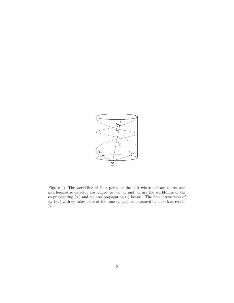
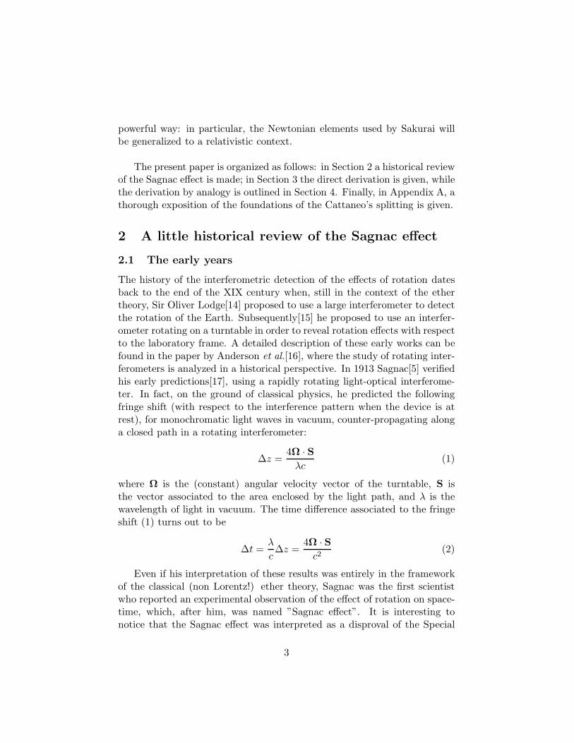
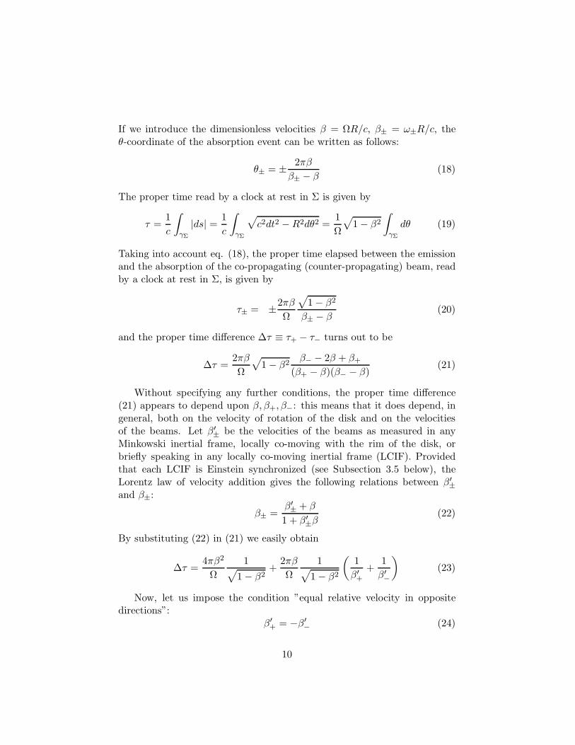
Figure 1: The world-line of Σ, a point on the disk where a beam source andinterferometric detector are lodged, is γΣ; γ+ and γ− are the world-lines of theco-propagating (+) and counter-propagating (-) beams. The first intersection ofγ+ (γ−) with γΣ takes place at the time τ+ (τ−), as measured by a clock at rest inΣ.

8

In particular, if we confine ourselves to a disk (z = const), the metric whichwe have to deal with is

ds2 = −c2dt2 + dr2 + r2dθ2 (11)

With respect to K, the disk (whose radius is R) rotates with angularvelocity Ω, and the world line γΣ of Σ is

γΣ ≡

x0 = ctx1 = r = Rx2 = θ = Ωt

(12)

or, eliminating t

γΣ ≡

x0 = cΩθ

x1 = Rx2 = θ

(13)

The world-lines of the co-propagating (+) and counter-propagating (-)beams emitted by the source at time t = 0 (when θ = 0) are, respectively:

γ+ ≡

x0 = cω+

θ

x1 = Rx2 = θ

(14)

γ− ≡

x0 = cω−

θ

x1 = Rx2 = θ

(15)

where ω+, ω− are their angular velocities, as seen in the central inertialframe4. The first intersection of γ+ (γ−) with γΣ is the event ”absorptionof the co-propagating (counter-propagating) beam after a complete roundtrip” (see figure 1). This event takes place when

1

Ωθ± =

1

ω±(θ± ± 2π) (16)

where the + (−) sign holds for the co-propagating (counter-propagating)beam. The solution of eq. (16) is:

θ± = ± 2πΩ

ω± − Ω(17)

4Notice that ω− is positive if |ω′

−| < Ω, null if |ω′

−| = Ω, and negative if |ω′

−| > Ω; see

eq.(22) below.

9

If we introduce the dimensionless velocities β = ΩR/c, β± = ω±R/c, theθ-coordinate of the absorption event can be written as follows:

θ± = ± 2πβ

β± − β(18)

The proper time read by a clock at rest in Σ is given by

τ =1

c

∫

γΣ

|ds| = 1

c

∫

γΣ

√c2dt2 −R2dθ2 =

1

Ω

√1− β2

∫

γΣ

dθ (19)

Taking into account eq. (18), the proper time elapsed between the emissionand the absorption of the co-propagating (counter-propagating) beam, readby a clock at rest in Σ, is given by

τ± = ±2πβ

Ω

√1− β2

β± − β(20)

and the proper time difference ∆τ ≡ τ+ − τ− turns out to be

∆τ =2πβ

Ω

√1− β2

β− − 2β + β+(β+ − β)(β− − β)

(21)

Without specifying any further conditions, the proper time difference(21) appears to depend upon β, β+, β−: this means that it does depend, ingeneral, both on the velocity of rotation of the disk and on the velocitiesof the beams. Let β′

± be the velocities of the beams as measured in anyMinkowski inertial frame, locally co-moving with the rim of the disk, orbriefly speaking in any locally co-moving inertial frame (LCIF). Providedthat each LCIF is Einstein synchronized (see Subsection 3.5 below), theLorentz law of velocity addition gives the following relations between β′

±and β±:

β± =β′± + β

1 + β′±β

(22)

By substituting (22) in (21) we easily obtain

∆τ =4πβ2

Ω

1√1− β2

+2πβ

Ω

1√1− β2

(1

β′+

+1

β′−

)(23)

Now, let us impose the condition ”equal relative velocity in oppositedirections”:

β′+ = −β′

− (24)

10

Such condition means that the beams are required to have the samevelocity (in absolute value) in every LCIF5, provided that every LICF isEinstein synchronized. If condition (24) is imposed, the proper time differ-ence (23) reduces to

∆τ =4πβ2

Ω

1√1− β2

=4πR2Ω

c2

(1− Ω2R2

c2

)−1/2

(25)

which is the relativistic Sagnac time difference.A very relevant conclusion follows. According to eq. (20), the beams take

different times - as measured by the clock at rest on the starting-ending pointΣ on the platform - for a complete round trip, depending on their velocitiesβ′± relative to the turnable. However, when condition (24) is imposed, the

difference ∆τ between these times does depend only on the angular Ω of thedisk, and it does not depend on the velocities of propagation of the beamswith respect the turnable.

This is a very general result, which has been obtained on the ground ofa purely kinematical approach. The Sagnac time difference (25) applies toany couple of (physical or even mathematical) entities, as long as a velocity,with respect the turnable, can be consistently defined. In particular, thisresult applies as well to photons (for which |β′

±| = 1) and to any kind ofclassical or quantum particles under the given conditions (or electromag-netic/acustic waves in presence of an homogeneous co-moving medium) 6.This fact evidences, in a clear and straightforward way, the universality ofthe Sagnac effect.

More in particular, the Sagnac time difference (25) also applies to theFourier components of the wave packets associated to a couple of matterbeams counter-propagating, with the same relative velocity, along the rim7.This remark is important to study the interferometric detectability of theSagnac effect, see Subsection 3.3 below.

3.2 The Sagnac effect as an empirical evidence of SRT

As we said in the Introduction, the Sagnac effect for electromagnetic wavesin vacuum was first interpreted by Sagnac himself as an experimental evi-dence of the physical existence of the classical (non relativistic) ether, and

5Or, differently speaking, with respect to any observer at rest in the ”relative space”(see below) along the rim of the platform.

6Provided that a group velocity can be defined.7Of course only matter beams are physical entities, while Fourier components are just

mathematical entities, to which no energy transport is associated.

11

an experimental disproval of SRT. Sagnac’s interpretation can be easily un-derstood, on the basis of the relativistic eq. (21), as a casual consequenceof a well known kinematical feature of light propagation through the ether.Indeed, the light velocity with respect to the ether (at rest in the centralIF) must be c in both directions; as a consequence, if we set β± = ±1 in eq.(21), the proper time difference ∆τ reduces to eq. (25); the latter, in turn,reduces, at first order approximation, to the time difference given in eq. (2),which was actually predicted and experimentally tested by Sagnac.

However, any non relativistic explanation completely fails for sublumi-nally travelling entities (such as matter waves, sound waves, electromagneticwaves in an homogeneous comoving medium, and so on). In fact, for sublu-minally travelling entities the vital condition is: ”equal relative velocity inopposite directions”. If this condition is expressed by eq. (24), where thelocal Einstein synchronization is explicitly required, the Sagnac proper timedifference (25) arises, as we carefully showed before.

On the contrary, if the condition ”equal relative velocity in opposite di-rections” is expressed by an analogous relation, in which the local Einsteinsynchronization is replaced by a synchronization borrowed from the globalsynchronization of the central IF (see Subsection 3.5), no time differencearises. Let us prove this claim.

Let ϕ± and ϑr± be the azimuthal coordinates of the co-rotating/counter-

rotating entity with respect to the central IF and the LCIF, respectively.These coordinates are related by the transformation

ϕ± = Ωt+ ϑr± (26)

Derivation of eq. (26) with respect to the central inertial time t gives

ω± = Ω+ ωr± (27)

where ω± ≡ dϕ±/dt is the angular velocity relative to the central IF, andωr± ≡ dϑr

±/dt is the angular velocity relative to the LCIF - provided it issynchronized by means of the central inertial time t.

Eq. (27), multiplied by R/c, takes the dimensionless form

β± = β + βr± (28)

which can replace eq. (22). Let us stress that both eqs. (22) and (28) arecorrect: the former refers to the local Einstein synchronization, the latterto the local synchronization according to the simultaneity criterium of thecentral IF.

12

Introducing eq. (28) into eq. (21), the proper time difference ∆τ reducesto

∆τ =2πβ

Ω

√1− β2

(β + βr−)− 2β + (β + βr

+)

βr−β

r+

=2πβ

Ω

√1− β2

βr− + βr

+

βr−β

r+

(29)If the vital condition ”equal relative velocity in opposite directions” is

expressed by eq.βr+ = −βr

− (30)

instead of eq. (24), it is plain from eq. (29) that no time difference arises:∆τ = 0 (Q.E.D.)

This calculation shows that the choice of the local Einstein synchroniza-tion is crucial even in non-relativistic motion. Indeed, the choice of theclassical eq. (28), instead of the relativistic eq. (22), could be naively pre-sumed as a reasonable approximation in non-relativistic motion: however,such a choice simply cancels the effect!

This shows that, according to a very appropriate remark by Dieks andNienhuis [46], the Sagnac effect is an experimental evidence of SRT, and anexperimental disproval of the classical (non relativistic) ether.

Remark. It could be always possible substitute eq. (24) with an al-ternative suitable condition, so that eq. (29) turns to be equal to eq. (25).Such a condition is:

βr− = −βr

+

1− β2

1− 2ββr+ − β2

(31)

But, of course, this is an extremely ”ad hoc” condition, which translates thesimple and expressive condition (24): it is clear that the physical interpre-tation of (31) is not as evident as that of (24).

3.3 Interferometric detectability of the Sagnac effect

With regard to the interferometric detection of the Sagnac effect, the crucialpoint is the following. Consider the Fourier components of the wave packetsassociated to a couple of matter beams counter-propagating, with the samegroup velocity, along the rim. Despite the lack of a direct physical meaningand energy transfer, the phase velocity of these Fourier components complieswith the Lorentz law of velocity addition (22 ), and is the same both theco-rotating and counter-rotating Fourier components. as a consequence, theSagnac time difference (25) also applies to any couple of Fourier componentswith the same phase velocity.

13

Moreover, the interferometric detection of the Sagnac effect requires thatthe wave packet associated to the matter beam should be sharp enough inthe frequency space, to allow the appearance, in the interferometric region,of an observable fringe shift.8 It may be worth recalling that:

(i) the observable fringe shift ∆z depends on to the phase velocity of theFourier components of the wave packet;

(ii) with respect to an Einstein synchronized LCIF, the velocity of ev-ery Fourier component of the wave packet associated to the matter beam,moving with the velocity (in absolute value) v ≡ c|β′

±|, is given by the DeBroglie expression vf = c2/v.

The consequent Sagnac phase shift, due to the relativistic time difference(25), is

∆Φ = 2π∆z = 2π(vfλ∆τ)=

8π2R2Ω

λv

(1− Ω2R2

c2

)−1/2

(32)

3.4 Comparing to some results found in the literature

As we mentioned, the Sagnac time delay for matter beams has been derivedby many authors in many different ways, but almost always in the first orderapproximation. However, digging into the literature, we eventually found,between the preliminary and the final version of this paper, a couple ofderivations of the Sagnac effect for matter beams in full SRT. In this sectionwe are going to compare these approaches to ours.

3.4.1 Dieks-Nienhuis’s approach

Dieks and Nienhuis[46] move from the standard Lorentz transformation fromthe LCIF to the central IF. In order to be as clear and self-consistent aspossible, we shall translate everything into our notations.

Consider two near events, happening along the rim, belonging to theworldline of the co-rotating/counter-rotating beam; let dx, dτ be the spaceand time separation between these events, as measured in an Einstein Syn-chronized LCIF. Then the corresponding time separation dt, as measured inthe central IF, is given by the usual Lorentz transformation

dt =

(dτ ± ΩRdx

c2

)(1− Ω2R2

c2

)−1/2

(33)

8That is, the Fourier components of the wave packet should have slightly differentwavelengths

14

where the + and − hold for the co-rotating and counter-rotating beams,respectively. Gluing together all the LCIFs, at the end of the round trip wehave (

1− Ω2R2

c2

)1/2

t± = τ(γ±)±ΩR

c2

∫

Ddx (34)

where D is the rim of the platform, as seen on the platform itself.The difference between the equations for the co-rotating and counter-

rotating beams is:

(1− Ω2R2

c2

)1/2

(t+ − t−) = τ(γ+)− τ(γ−) +2ΩR

c2

∫

Ddx (35)

In the derivation given by Dieks and Nienhuis, two hypotheses play avital role in order to get the correct conclusion: (i) the integration domain D

is 2πR(1− Ω2R2

c2

)−1/2; (ii) τ(γ+) = τ(γ−) =

(2πRv′

) (1− Ω2R2

c2

)−1/2, where

v′ is the relative velocity (in absolute value) of both the co-rotating and thecounter-rotating beam (as a consequence, τ(γ+)− τ(γ−) = 0).

Let us briefly comment these hypotheses: of course, the two hypothesesare correct, but both deserve further remarks.

First of all, we could say that hypothesis (i) is unnecessary: indeed, ourderivation of the Sagnac effect does not depend on the hyperbolic feature ofthe space geometry of the disk (see Subsection 4.2 and Appendix A.14). Onthe other hand, this hypothesis establishes a very interesting link betweenthe (observable) Sagnac time delay and the (unobservable) lengthening ofthe rim of the rotating platform, which, in turn, depends on the peculiarspace geometry of the disk. This is a challenge to those authors (see forinstance [25],[47]) who try to conciliate the Sagnac time delay with theEuclidean space geometry of the disk.

With respect to hypothesis (ii), it should be stressed that it seems tochallenge the well known Hafele-Keating experiment[48], and its theoreticalinterpretation[49],[50]. As a matter of fact, the proper time of the twoHafele-Keating aircrafts are actually different. Let us stress that the latterstatement is true even in the limit of extremely slow motion with respect tothe platform (see [49] for details).

3.4.2 Malykin’s approach

The long review paper by Malykin[51] (almost 300 references!) starts withthe remark that the Sagnac effect for matter beams ”is explained in severaltotally different ways”, but - strangely enough - most of them give ”correct

15

results despite their obvious incorretness”. After a wide overview of these”incorrect explanations”, the author provides his attempt of solution onthe basis of the relativistic law of velocity composition. This approach isthe only one that turns out to be similar to ours; also the problem of theinterferometric detection of the Sagnac effect is taken into account. Ofcourse, this leads to the issue of the kinematical behavior of both the phasevelocity and the group velocity. Here some misinterpretations and confusionsarise. In particular, the author tries to show that ”both the group velocityand the phase velocity have identical translational properties during thetransition from the frame of reference K [the central IF] to the frame ofreference K’ [the LCIF]”.

Actually, the group velocity behaves contrary to the phase velocity withrespect to the (local) Lorentz transformation group. However, this has noconsequences on the interferometric detection of the Sagnac effect, becausethe only relevant requirement is that, with respect to any Einstein syn-chronized LCIF: (i) the group velocities should be the same; (ii) the phasevelocities of the Fourier components should be the same. This is exactlywhat happens: the transformation properties have no role. Anyway, weagree with Malykin when he says that ”the Sagnac effect constitutes a kine-matical effect of SRT; (...) all explanations of the Sagnac effect are incorrectexcept the relativistic one”. We also agree with his final remark: the exis-tence of a large number of incorrect explanations which give correct results(at least in first approximation) depends on the fact that the Sagnac effectis a first-order effect in v/c.

3.4.3 Anderson, Stedman and Bilger’s approach

It is interesting to compare our results to this approach, even though An-derson, Stedman and Bilger’s results[40],[16] are confined to a first orderapproximation. Indeed, they find, at first order approximation, the follow-ing time difference:

∆t =4Ω · Sv2

(36)

and the following phase shift:

∆Φ =8πΩ · S

λv(37)

where v is the ”undragged” velocity of the beams. Of course, the timedifference (36) is not in agreement with the first order approximation (withrespect to β = ΩR/c) of eq. (25). However, it is consistent with the first

16

order approximation of eq. (21) provided that β+ = −β− ≡ v/c: thisrepresents a completely different physical situation, in which the two beamsare injected into the rotating platform (tangentially to the rim) in oppositedirections with the same velocity with respect to the central inertial frame.

On the other hand, the phase shift (37), which is the only observablequantity through an interferometric device, is not in agreement with thephysical situation considered by these authors. However, it is worthwhile tonotice that, oddly enough, it perfectly agrees with the first order approxi-mation of eq. (32).9

3.4.4 Ashby’s approach

The best approach that we know, at first order approximation, is the onesuggested in this book by Ashby[52]. The peculiarity of this approach is thatit is independent of the shape of the loop: this is a very important featurewhen dealing with the Global Positioning System (GPS). In particular, it isshown that the Sagnac time delay depends only on the area swept out by theelectromagnetic pulse, as it travels from the GPS transmitter to the receiver,projected onto the terrestrial equatorial plane. A great care is devoted tosynchronization problems: this issue is in complete agreement with our fullyrelativistic approach (see Subsection 3.5, below).

3.5 Synchronization in a LCIF: a free choice

As pointed out by Rizzi-Serafini[49], in a local or global inertial frame (IF)the synchronization is not ”given by God”, as often both relativistic andanti-relativistic authors assume, but it can be arbitrarly chosen within thesynchronization gauge

t′ = t′ ( t, x1, x2, x3)x′i = xi

(38)

The synchronization gauge (38) is a subset of the Cattaneo gauge (56) (seeAppendix A.4), which is the set of all the possible parameterizations of thegiven physical inertial frame (IF). In eq. (38) the coordinates (t, xi) areEinstein coordinates, and (t′, x′i) are re-synchronized coordinates of the IFunder consideration. Of course, the IF turns out to be optically isotropicif and only if it is parameterized by Einstein coordinates (t, xi). Then the

9If condition (24) is imposed, eq. (36) is wrong and eq. (37) is right.

17

following question arises: if the parameterization (in particular the synchro-nization) of a LCIF is a matter of choice, which is the most profitable choicein order to describe the Sagnac effect?

Since the synchronization gauge (38) is too general for a clear and usefuldiscussion, it is advantageous to introduce a suitable subset of the synchro-nization gauge, allowing a more meaningful and clearer discussion. Such asub-gauge actually exists; it has been introduced by Selleri[18],[19]. Let usbriefly summarize the Selleri’s gauge.

Let K be a ”formally privileged” IF, in which an isotropic synchroniza-tion (that is Einstein synchronization) is assumed by stipulation; and let Sbe a (generally anisotropic) IF moving along the x′1 = x1 axis with dimen-sionless velocity β with respect to K. The Selleri gauge is defined by

t′ = t+ Γ(β)

c xx′i = xi

(39)

where Γ(β) is an arbitrary function of β. It is convenient to write thisfunction as follows:

Γ(β) ≡ β + e1(β)cγ−1 (40)

The function e1(β) is the Selleri’s ”synchronization parameter”, which, inprinciple, can be arbitrary chosen. Any choice of the function e1(β) is achoice of the synchronization in the IF under consideration; in principle, thesynchronization can be freely chosen inside the Selleri gauge (39). In partic-ular, the synchrony choice e1(β)

.= −βγ/c (that is Γ(β)

.= 0) gives the stan-

dard Einstein synchronization, which is ”relative” (that is frame-dependent);whereas the synchrony choice e1(β)

.= 0 gives the Selleri synchronization,

which is ”absolute” (that is frame-independent).The term ”absolute” sounds rather eccentric in a relativistic framework,

but it simply means that the Selleri simultaneity hypersurfaces t′ = const(contrary to the the Einstein simultaneity hypersurfaces t = const) define aframe-invariant foliation of space-time - which is nothing but the Einsteinfoliation of the particular IF K assumed (by stipulation, once and for all)as optically isotropic for any choice of the synchronization parameter.

According to Selleri, the synchronization is a matter of convention in thecase of translation, but not in the case of rotation: when rotation is takeninto account, the synchronization parameter e1 is forced to take the valuezero. On the contrary, as it is shown in [49], the choice of e1 is not compelledby any empiric evidence: that is, also when rotation is taken into account,no physical effect can discriminate the Selleri’s synchrony choice e1(β)

.= 0

from the Einstein’s synchrony choice e1(β).= −βγ/c.

18

Therefore, we have the opportunity of taking a very pragmatic view:both Selleri’s ”absolute” synchronization and Einstein relative synchroniza-tion can be used, depending on the aims and circumstances. In particular,(i) if we look for a global synchronization on the rotating platform, Selleri’s”absolute” synchronization is required; (ii) if we look for a plain kinematicalrelationship between local velocities, Einstein synchronization is required inany LCIF.

Let us outline the advantages of the local Einstein synchronization on arotating platform. First, let us recall[49] that the local isotropy or anisotropyof the velocity of light in a LCIF is not a fact, with a well defined ontologicalmeaning, but a convention which depends on the synchronization chosen inthe LCIF. Of course the velocity of light has the invariant value c in everyLCIF, both in co-rotating and counter-rotating direction, if and only if theLCIF are Einstein-synchronized. We are aware that this statement is notshared by some authors [24], [18], [19], [53], so we shall try to suggest a moresignificant one. As showed in Subsection. 3.1, the Sagnac time difference(25) holds for two beams travelling in opposite directions, along the rim, withthe same velocity with respect the turnable. This is a plain and meaningfulcondition: but it must be stressed that this condition requires that everyLCIF should be Einstein-synchronized . Of course this condition could betranslated also in the Selleri’s absolute synchronization, but it would result ina very artificial and convoluted requirement. Only Einstein synchronizationallows the clear and meaningful requirement: ”equal relative velocity inopposite directions”,10 as we showed in the Remark of Subsection 3.2.

4 The Sagnac effect from an analogy with the Aharonov-

Bohm effect

In this section we shall give another derivation of the Sagnac time differencefor relativistic material beams counter-propagating on a rotating disk[54].This derivation is based on a (formal) analogy with the Aharonov-Bohmeffect which has been outlined by Sakurai[7]. However, Sakurai’s approach,which rests upon the use of relativistic and Newtonian elements, gives onlythe first order (in β) approximation of Sagnac time difference (25). We wantto show that, using Cattaneo’s splitting techniques, it is possible to state theanalogy between the Aharonov-Bohm effect and the Sagnac effect in a fullyrelativistic context, getting rid of the Newtonian elements and recovering the

10Formally expressed by condition (24).

19

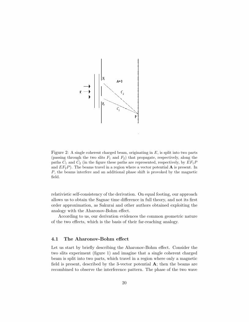
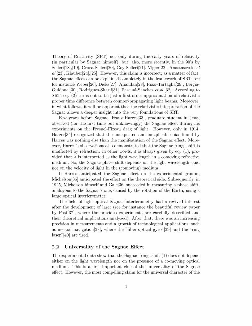
Figure 2: A single coherent charged beam, originating in E, is split into two parts(passing through the two slits F1 and F2) that propagate, respectively, along thepaths C1 and C2 (in the figure these paths are represented, respectively, by EF1Pand EF2P ). The beams travel in a region where a vector potential A is present. InP , the beams interfere and an additional phase shift is provoked by the magneticfield.

relativistic self-consistency of the derivation. On equal footing, our approachallows us to obtain the Sagnac time difference in full theory, and not its firstorder approximation, as Sakurai and other authors obtained exploiting theanalogy with the Aharonov-Bohm effect.

According to us, our derivation evidences the common geometric natureof the two effects, which is the basis of their far-reaching analogy.

4.1 The Aharonov-Bohm effect

Let us start by briefly describing the Aharonov-Bohm effect. Consider thetwo slits experiment (figure 1) and imagine that a single coherent chargedbeam is split into two parts, which travel in a region where only a magneticfield is present, described by the 3-vector potential A; then the beams arerecombined to observe the interference pattern. The phase of the two wave

20

functions, at each point of the pattern, will be modified, with respect to thecase of free propagation (A = 0), by the magnetic potential. The magneticpotential-induced phase shift has the form[8]

∆Φ =e

c~

∮

CA · dr = e

c~

∫

SB · dS (41)

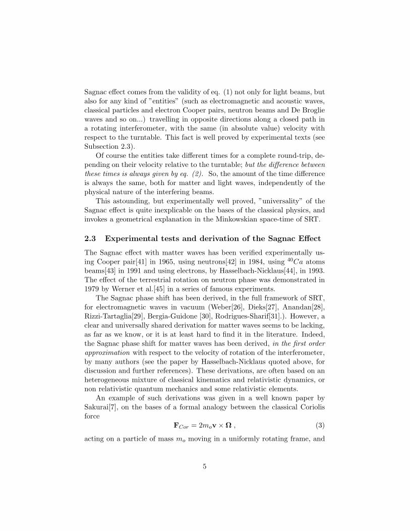
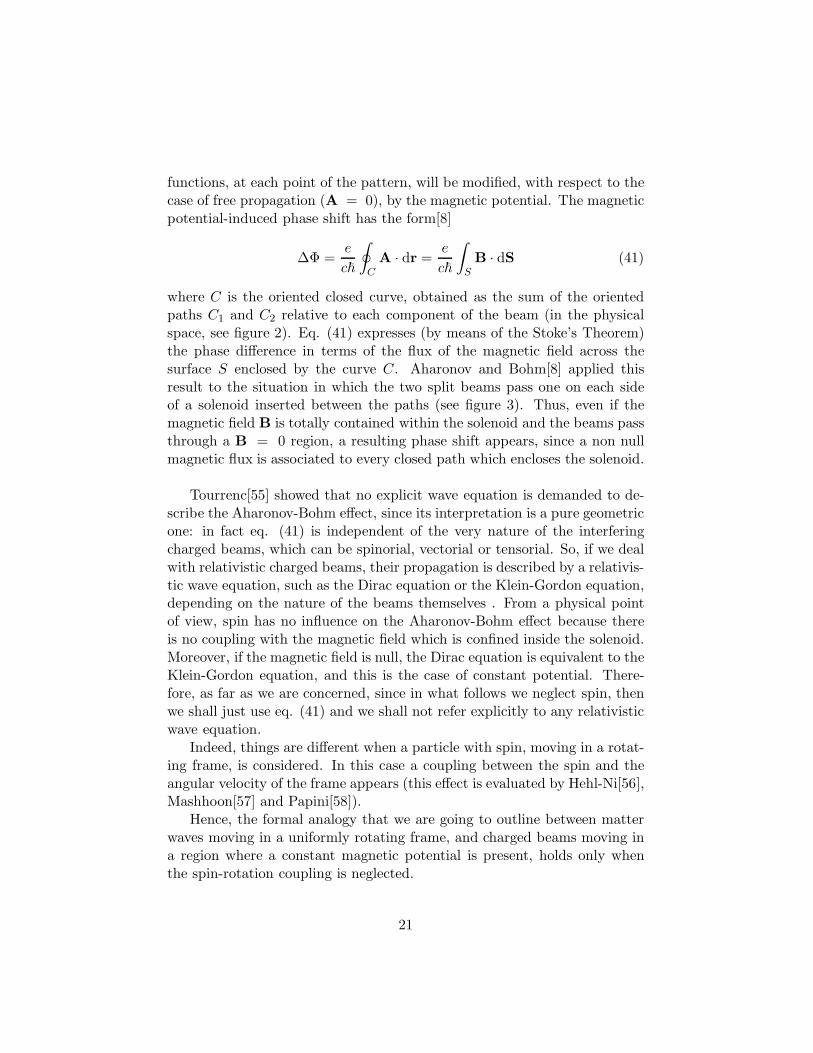
where C is the oriented closed curve, obtained as the sum of the orientedpaths C1 and C2 relative to each component of the beam (in the physicalspace, see figure 2). Eq. (41) expresses (by means of the Stoke’s Theorem)the phase difference in terms of the flux of the magnetic field across thesurface S enclosed by the curve C. Aharonov and Bohm[8] applied thisresult to the situation in which the two split beams pass one on each sideof a solenoid inserted between the paths (see figure 3). Thus, even if themagnetic field B is totally contained within the solenoid and the beams passthrough a B = 0 region, a resulting phase shift appears, since a non nullmagnetic flux is associated to every closed path which encloses the solenoid.

Tourrenc[55] showed that no explicit wave equation is demanded to de-scribe the Aharonov-Bohm effect, since its interpretation is a pure geometricone: in fact eq. (41) is independent of the very nature of the interferingcharged beams, which can be spinorial, vectorial or tensorial. So, if we dealwith relativistic charged beams, their propagation is described by a relativis-tic wave equation, such as the Dirac equation or the Klein-Gordon equation,depending on the nature of the beams themselves . From a physical pointof view, spin has no influence on the Aharonov-Bohm effect because thereis no coupling with the magnetic field which is confined inside the solenoid.Moreover, if the magnetic field is null, the Dirac equation is equivalent to theKlein-Gordon equation, and this is the case of constant potential. There-fore, as far as we are concerned, since in what follows we neglect spin, thenwe shall just use eq. (41) and we shall not refer explicitly to any relativisticwave equation.

Indeed, things are different when a particle with spin, moving in a rotat-ing frame, is considered. In this case a coupling between the spin and theangular velocity of the frame appears (this effect is evaluated by Hehl-Ni[56],Mashhoon[57] and Papini[58]).

Hence, the formal analogy that we are going to outline between matterwaves moving in a uniformly rotating frame, and charged beams moving ina region where a constant magnetic potential is present, holds only whenthe spin-rotation coupling is neglected.

21

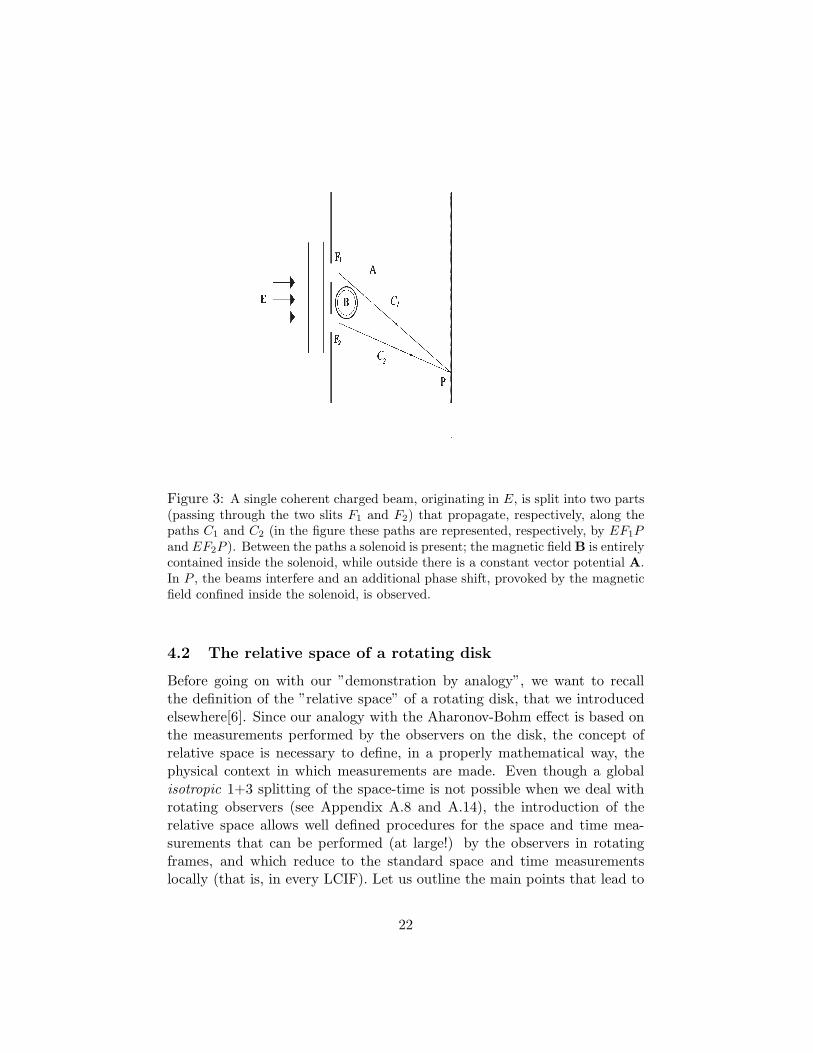
Figure 3: A single coherent charged beam, originating in E, is split into two parts(passing through the two slits F1 and F2) that propagate, respectively, along thepaths C1 and C2 (in the figure these paths are represented, respectively, by EF1Pand EF2P ). Between the paths a solenoid is present; the magnetic fieldB is entirelycontained inside the solenoid, while outside there is a constant vector potential A.In P , the beams interfere and an additional phase shift, provoked by the magneticfield confined inside the solenoid, is observed.

4.2 The relative space of a rotating disk

Before going on with our ”demonstration by analogy”, we want to recallthe definition of the ”relative space” of a rotating disk, that we introducedelsewhere[6]. Since our analogy with the Aharonov-Bohm effect is based onthe measurements performed by the observers on the disk, the concept ofrelative space is necessary to define, in a properly mathematical way, thephysical context in which measurements are made. Even though a globalisotropic 1+3 splitting of the space-time is not possible when we deal withrotating observers (see Appendix A.8 and A.14), the introduction of therelative space allows well defined procedures for the space and time mea-surements that can be performed (at large!) by the observers in rotatingframes, and which reduce to the standard space and time measurementslocally (that is, in every LCIF). Let us outline the main points that lead to

22

the definition of the relative space.

The world-lines of each point of the rotating disk are time-like helixes(whose pitch, depending on Ω, is constant), wrapping around the cylindricalsurface r = const, with r ∈ [0, R]. These helixes fill, without intersecting,the whole space-time region defined by r ≤ R < c/Ω; they constitute atime-like congruence Γ which defines the rotating frame Krot, at rest withrespect to the disk.11 Let us introduce the coordinate transformation

x′0 = ct′ = ctx′1 = r′ = rx′2 = ϑ′ = ϑ− Ωtx′3 = z′ = z

. (42)

The coordinate transformation xµ → x′µ defined by (42) has a kine-matical meaning, namely it defines the passage from a chart adapted to theinertial frame K to a chart adapted to the rotating frame Krot. In the chartx′µ the metric tensor is written in the form12:

g′µν =

−1 + Ω2r2

c20 Ωr2

c 00 1 0 0

Ωr2

c 0 r2 00 0 0 1

(43)

This is the so called Born metric, and in the classic textbooks (see, forinstance Landau-Lifshits[59] and Møller [60])it is commonly presented asthe space-time metric in the rotating frame of the disk.

Moreover, we can calculate the space metric tensor γ′ij of the congruencewhich defines Krot (see Appendix A.6 and A.14):

γ′ij = g′ij − γ′iγ′j =

1 0 0

0 r2

1−Ω2r2

c2

0

0 0 1

. (44)

As it is shown explicitly in Appendix A.14, the congruence Γ of time-likehelixes, wrapping around the cylindrical hypersurfaces σr (r = cost ∈]0, R]),defines a Killing field not in M4, but on the submanifolds σr ⊂ M4.13

11The constraint R < c/Ω simply means that the velocity of the points of the disk

cannot reach the speed of light.12For the sake of simplicity, we substitute r′ = r, from (42) II .13M4, which is a differential manifold, is the (model of the) physical space-time (see

Appendix A.1).

23

Consequently, we can point out the following interesting property. LetTp = Θp ⊕ Σp be the tangent space to M4 in p, where Θp, and Σp are thelocal time direction and the local space platform (see Appendix A.6). Thenthe splitting Tp = Θp ⊕ Σp and the space metric tensor γ′ij(p) are invariantalong the lines of Γ. It is then possible to define a one-parameter group ofdiffeomorphisms with respect to which both the splitting Tp = Θp ⊕Σp andthe space metric tensor γ′ij(p) are invariant. The lines of Γ constitute thetrajectories of this ”space ⊕ time isometry”. This important property sug-gests a procedure to define an extended 3-space, which we shall call ‘relativespace’ : it will be recognized as the only space having an actual physicalmeaning from an operational point of view, and it will be identified as the’physical space of a rotating platform’.

Definition. Each element of the relative space is an equivalence classof points and of space platforms, which verify this equivalence relation:

RE: “ Two points (two space platforms) are equivalent if they belong tothe same line of the congruence ”.

That is, the relative space is the ”quotient space” of the world tube ofthe disk, with respect to the equivalence relation RE, among points andspace platforms belonging to the lines of the congruence Γ. This definitionsimply means that the relative space is the manifold whose ”points” are thelines of the congruence.

We stress that it is not possible to describe the relative space in termsof space-time foliation, i.e. in the form x0 = const, where x0 is an appro-priate coordinate time, because the space of the disk, as we show in theAppendix A.14, is not time-orthogonal. Hence, thinking of the space of thedisk as a sub-manifold or a subspace embedded in the space-time is mis-leading and meaningless. The best we can do, if we long for some kind ofvisualization, is to think of the relative space as the union of the infinites-imal space platforms, each of which is associated, by means of the requestof M -orthogonality, to one and only one line of the congruence.

In the relative space, an observer can perform measurements of space andtime. His reference frame, defined by the relative space, coincides everywherewith the local rest frame of the rotating disk. As a consequence, spacemeasurements are performed on the bases of the spatial metric (44), without

24

caring of time, since γ′ij does not depend on time14. Moreover, the observercan measure time intervals using his own standard clock, on which he readsthe proper time.

4.3 The Sagnac effect in the relative space

Now, we are going to describe the interference process of material beamscounter-propagating in a rotating ring interferometer, from the viewpointof the rotating frame. As we showed before, the physical space of the ro-tating frame is the relative space. Then, a formal analogy, between matterbeams counter-propagating in the rotating frame, and charged beams prop-agating in a region where a magnetic potential is present, can be outlinedon the bases of Cattaneo’s formulation of the ”relative standard dynamics”.In particular, the equation of motion of a particle relative to the rotatingframe Krot, can be given in terms of the Gravitoelectromagnetic (GEM)fields (see Appendix A.13). The introduction of the GEM fields leads to ananalogy between the Aharonov-Bohm effect and the Sagnac effect in a fullyrelativistic context.

In eq. (114), the general form of the standard relative equation of motionof a particle is given in terms of the gravito-electric field EG, the gravito-magnetic field BG and the external fields.15 In particular, in eq. (114) agravito-magnetic Lorentz force appears

Fi = mγ0

(v

c× BG

)

i

(45)

On the bases of this description, we want to apply the formal analogybetween the gravito-magnetic and magnetic field to the phase shift inducedby rotation on a beam of massive particles which, after being split, propagatein two opposite directions along the rim of a rotating disk. When they arerecombined, the resulting phase shift is the manifestation of the Sagnaceffect.

To this end, let us consider the analogue of the phase shift (41) for thegravito-magnetic field

∆Φ =2mγ0c~

∮

CAG · dr = 2mγ0

c~

∫

SBG · dS (46)

14This is a consequence of the stationarity of the rotating frame.15For instance, the constraints that force the particle to move along the rim of the disk

are ”external fields”.

25

which is obtained on the bases of the formal analogy between eq. (45) andthe magnetic force (4):

e

cB → mγ0

cBG (47)

To calculate the phase shift (46) we must express explicitly the gravito-magnetic potential and field corresponding to the congruence Γ relative tothe rotating frame Krot. In particular (see A.14) the non null componentsof the vector field γ(x), evaluated on the trajectory R = const along whichboth beams propagate, are:

γ0.= 1√

−g00= γ

γ0.=

√−g00 = γ−1

γ2 = γϑ.= gϑ0γ

0 = γΩR2

c

(48)

where γ =(1− Ω2R2

c2

)− 1

2

.

For the gravitomagnetic potential we then obtain

AG2 = AG

ϑ.= c2

γϑγ0

= γ2ΩR2c (49)

As a consequence, the phase shift (46) becomes

∆Φ =2m

c~γ

∫ 2π

0AG

ϑ dϑ =2m

c~γ

∫ 2π

0

(γ2ΩR2c

)dϑ = 4π

m

~ΩR2γ (50)

According to Cattaneo’s terminology (see Appendix A.10), the propertime is the ”standard relative time” for an observer on the rotating platform;the proper time difference corresponding to (50) is obtained according to

∆τ =∆Φ

ω=

~

E∆Φ =

~

mc2∆Φ (51)

and it turns out to be

∆τ = 4πΩR2γ

c2≡ 4πR2Ω

c2(1− Ω2R2

c2

)1/2 (52)

Eq. (52) agrees with the proper time difference (25) due to the Sagnac ef-fect, which, as we pointed out in Subsection 2.2, corresponds to the timedifference for any kind of matter entities counter-propagating in a uniformlyrotating disk. As we stressed before, this time difference does not dependon the standard relative velocity of the particles and it is exactly twice the

26

time lag due to the synchronization gap arising in a rotating frame.

Remark In order to generalize Sakurai’s procedure, which refers toneutron beams, in this section we always referred to material beams. How-ever, the procedure that leads to the time difference (52) can be carried outalso referring to light beams. Actually, in Appendix A.12, we show that arelative standard mass of a photon m

.= hν

c2can be defined. Consequently,

the relative formulation of the equation of motion of a photon, is describedin a way analogous to that of a material particle, and the procedure thatwe have just outlined can be applied in a straightforward way to masslessparticles too.

The phase shift (50) can be expressed also as a function of the area S ofthe surface enclosed by the trajectories:

∆Φ = 2β2SΩm

~

γ2

γ − 1= 2

m

~SΩ (γ + 1) (53)

where β = ΩRc and

S =

∫ R

0

∫ 2π

0

rdrdϑ√1− Ω2r2

c2

= 2πc2

Ω2

(1−

√1− Ω2R2

c2

)= 2π

c2

Ω2

(γ − 1

γ

)

(54)We notice that (53) reduces to (8)16, only in the first order approximationwith respect to ΩR

c , i.e. when γ → 1: the formal difference between (53)and (8) is due to the non Euclidean features of the relative space (see A.14).

5 Conclusions

The relativistic Sagnac effect has been deduced, by means of two derivations.In the first part of this paper, a direct derivation has been outlined on

the bases of the relativistic kinematics. In particular, only the law of veloc-ity addition has been used to obtain the Signac time difference and to show,in a straightforward way, its independence from the physical nature and thevelocities (relative to the turntable) of the interfering beams.

In the second part of this paper, an alternative derivation has been pre-sented. In particular, the formal analogy outlined by Sakurai, which ex-plains the effect of rotation using a ”ill-assorted” mixture of non-relativistic

16Apart a factor 2, whose origin has been explained in the footnote 2 in Subection 2.3.

27

quantum mechanics, newtonian mechanics (which are Galilei-covariant) andintrinsically relativistic elements17 (which are Lorentz-covariant), has beenextended to a fully relativistic treatment, using the 1+3 Cattaneo’s split-ting technique. The space in which waves propagate has been recognized asthe relative space of a rotating frame, which turns out to be non-Euclidean.Using this splitting technique, we have generalized the Newtonian elementsused by Sakurai to a fully relativistic context, where we have been ableto adopt relativistic quantum mechanics. In this way, we have obtained aderivation of the relativistic Sagnac time difference (whose first order ap-proximation coincides with Sakurai’s result) in a self-consistent way.

Both derivations are carried out in a fully relativistic context, whichturns out to be the natural arena where the Sagnac effect can be explained.Indeed, its universality can be clearly understood as a purely geometricaleffect in the Minkowski space-time of SRT, while it is hard to grasp in thecontext of classical physics.

17Indeed, the lack of self-consistency, due to the use of this ”odd mixture”, is presentnot only in Sakurai’s derivation, but also in all the known approaches based on the formalanalogy with the Aharonov-Bohm effect.

28

A Appendix: Space-Time Splitting and Cattaneo’s

Approach

The tools for splitting space-time have had a great (even though heteroge-nous) development in the years, and they have been used in various appli-cation in General Relativity(GR). Indeed, the common aim of the differentapproaches to splitting techniques is the description of what is measured by atest family of observers, moving along certain curves in the four-dimensionalcontinuum.

In this way, locally, along the world-lines of these observers, space+timemeasurements can be recovered, and the description of the physical phe-nomena borrowed from SRT can be transferred into GR.

There are various approach to splitting of space-time, and a great workhas be done, recently, to describe everything in a common framework, evi-dencing the relationships among the different techniques[61],[62],[63].

Probably, the most well known and used splitting is the so called ”ADMsplitting”[64] (see also Gravitation[65]), which is based on the use of a familyof space-like hypersurfaces (”slicing” point of view); on the other hand, theapproach based on a congruence of time-like observers (”threading” point ofview) was developed independently by various authors, such as Cattaneo[9],[10], [11], [12], [13], Møller[60] and Zel’manonv[66] during the 1950’s, butit has remained greatly unknown for a long time, also because some of theoriginal works were not published in English, but in Italian, French or Rus-sian. Because of the pedagogical aim that we have in writing this paper, wedecided to present here a very introductory primer to the original Cattaneo’sworks on splitting of space-time. After the publication of his works, duringthe 1950’s and 1960’s, a lot of work has been done, in order to improve histechniques (see [61],[62],[63], and reference therein). However, we believethat the foundations of his approach can be understood, in the easiest andmost enlightening way, by referring to his original works. Moreover, sinceour aim is not historical but pedagogical, we shall translate his ”relativeformulation of dynamics” in terms of the Gravitoelectromagnetic analogy:indeed, we exploited this analogy in our derivation of the Sagnac effect start-ing from the Aharonov-Bohm effect.

A.1 It is important to define correctly the properties of the physicalframes with respect to which we describe the measurement processes. Weshall adopt the most general description, which takes into account non-inertial frames (for instance rotating frames) in SRT, and arbitrary framesin GR.

29

The physical space-time is a (pseudo)riemannian manifold M4, that is apair (M,g), where M is a connected 4-dimensional Haussdorf manifold andg is the metric tensor18. Let the signature of the manifold be (−1, 1, 1, 1).Suitably differentiability condition, on both M and g, are assumed.

A.2 A physical reference frame is a time-like congruence Γ: the set ofthe world lines of the test-particles constituting the ”reference fluid”19. Thecongruence Γ is identified by the field of unit vectors tangent to its worldlines. Briefly speaking, the congruence is the (history of the) physical frameor the reference fluid (they are synonymous).

A.3 Let xµ = (x0, x1, x2, x3) be a system of coordinates in the neigh-borhood of a point p ∈ M; these coordinates are said to be admissible (withrespect to the congruence Γ) when20

g00 < 0 gijdxidxj > 0 (55)

Thus the coordinates x0 = var can be seen as describing the world lines ofthe ∞3 particles of the reference fluid.

A.4 When a reference frame has been chosen, together with a set ofadmissible coordinates, the most general coordinates transformation whichdoes not change the physical frame, i.e. the congruence Γ, has the form[60],[67],[9]:

x′0 = x′0(x0, x1, x2, x3)x′i = x′i(x1, x2, x3)

(56)

with the additional condition ∂x′0/∂x0 > 0, which ensures that the changeof time parameterization does not change the arrow of time. The coordinatestransformation (56) is said to be internal to the physical frame Γ, or internal

18The riemannian structure implies that M is endowed with an affine connection com-patible with the metric, i.e. the standard Levi-Civita connection.

19The concept of ’congruence’ refers to a set of word lines filling the manifold, or somepart of it, smoothly, continuously and without intersecting.The concept of ’reference fluid’ is an obvious generalization of the ’reference solid’ whichcan be used in flat space-time, when the test particles constitute a global inertial frame.In this case, their relative distance remains constant and they evolve as a rigid frame.

However: (i) in GR test particles can be subject to a gravitational field (curvature ofspace-time); (ii) in SRT test particles can be subject to an acceleration field. In bothcases, global inertiality is lost and tidal effects arise, causing a variation of the distancebetween them. So we must speak of ”reference fluid”, dropping the compelling request ofclassical rigidity.

20Greek indices run from 0 to 3, Latin indices run from 1 to 3.

30

gauge transformation, or more simply Cattaneo’s gauge transformation.

A.5 An “observable” physical quantity is in general frame-dependent,but its physical meaning requires that it cannot depend on the particular pa-rameterization of the physical frame: in brief, it cannot be gauge-dependent.Then a problem arises. In the mathematical model of GR, physical quan-tities are expressed by absolute entities21, such as world-tensors, and thephysical laws, according to the covariance principle, are just relations amongthese entities. So, given a reference frame, how do we relate these absolutequantities to the relative, i.e. reference-dependent, ones? And how do werelate world equations to reference-dependent ones? In other words: how dowe relate, by a suitable 1+3 splitting, the mathematical model of space-timeto the observable quantities which are relative to a reference frame?

A.6 In order to do that, we are going to introduce the projectiontechnique developed by Cattaneo. Let γ(x) be the field of unit vectorstangent to the world lines of the congruence Γ. Given a time-like congruenceΓ it is always possible to choose a system of admissible coordinate so thatthe lines x0 = var coincide with the lines of Γ; in this case, such coordinatesare said to be ‘adapted to the physical frame’ defined by the congruence Γ.

Being gµνγµγν = −1, we get

γ0 = 1√

−g00

γi = 0

γ0 =

√−g00γi = gi0γ

0 (57)

In each point p ∈ M, the tangent space Tp can be split into the directsum of two subspaces: Θp, spanned by γα, which we shall call local timedirection of the given frame, and Σp, the 3-dimensional subspace whichis supplementary (orthogonal) with respect to Θp; Σp is called local spaceplatform of the given frame. So the tangent space can be written as thedirect sum

Tp = Θp ⊕ Σp (58)

A vector v ∈ Tp can be projected onto Θp and Σp using the time projectorγµγν and the space projector γµν

.= gµν − γµγν :

vµ = PΘ (v)

.= γµγνv

ν

vµ = PΣ (v).= vµ − vνγνγµ = (gµν − γµγν) v

ν = γµνvν (59)

21‘Absolute’ means ‘independent of any reference frame’.

31

Notation The superscripts −,∼ denote respectively a time vector and aspace vector, or more generally, a time tensor and a space tensor (see below).

Equation (59) defines the natural splitting of a vector. The tensors γµγνand γµν are called time metric tensor and space metric tensor, respectively.In particular, for each vector v it is possible to define a ‘time norm’ ‖v ‖Θand a ‘space norm’ ‖v ‖Σ as follows:

‖v ‖Θ.= vρv

ρ = γργνvν (γργµv

µ) = γµγνvµvν = (γµv

µ)2 ≤ 0 (60)

‖v ‖Σ.= vν v

ν = γµνvµ(vν − γηγ

νvη) = γµνvµvν ≥ 0 (61)

For a tensor field T ∈ Tp, every index can be projected onto Θp and Σp

by means of the projectors defined before:

PΘ(T...µ...).= γµγνT

...ν... PΣ(T...µ...).= γµνT

...ν... (62)

A tensor field of order two can be split into the sum of four tensors

PΣΣ ( tµν ).= γµργνηt

ρη PΣΘ ( tµν ).= γµργνγηt

ρη

PΘΣ ( tµν ).= γµγργνηt

ρη PΘΘ ( tµν ).= γµγνγργηt

ρη (63)

belonging to four orthogonal subspaces

Tp ⊗ Tp = (Σp ⊗ Σp)⊕ (Σp ⊗Θp)⊕ (Θp ⊗ Σp)⊕ (Θp ⊗Θp) (64)

In particular, every tensor belonging entirely to Σp⊗Σp is called a spacetensor and every tensor belonging to Θp ⊗ Θp is called a time tensor. Ofcourse, these entities have a tensorial behavior only with respect to the groupof the coordinates transformation (56). It is straightforward to extend theseprocedures and definitions to tensors of generic order n (see below) .

Remark 1 The natural splitting of a tensor is gauge-independent: itdepends only on the physical frame chosen. The projection technique givesgauge-invariant quantities that can have an operative meaning in our phys-ical frame; namely, they represent the objects of our measurements.

Remark 2 In Γ-adapted coordinates, a time vector v ∈ Θp is character-ized by the vanishing of its controvariant space components (vi = 0); a spacevector v ∈ Σp by the vanishing of its covariant time component (v0 = 0). Asa generalization: (i) a given index of a tensor T is called a time-index if allthe tensor components of the type T .i.

... (i ∈ [1, 2, 3]) vanish; (ii) a given index

32

of a tensor T is called a space-index if all the tensor components of the typeT ....0. vanish. For a time tensor, i.e. for a tensor belonging to Θp ⊗ ... ⊗Θp,

property (i) holds for all its indices; for a space tensor, i.e. a tensor belong-ing to Σp ⊗ ...⊗ Σp, property (ii) holds for all its indices.

A.7 To formulate the physical equations relative to the frame Γ, weneed the following differential operator

∂µ.= ∂µ − γµγ

0∂0 (65)

which is called transverse partial derivative. It is a ”space vector” and (itsdefinition) is gauge-invariant.

It is easy to show that, for a generic scalar field ϕ(x) we obtain:

PΣ(∂µϕ) = ∂µϕ (66)

So ∂µ defines the transverse gradient, i.e. the space projection of the localgradient.

The projection technique that we have just outlined allows to calculatethe projections of the Christoffel symbols. It is remarkable that the totalspace projections read

PΣΣΣ(µν, λ) =1

2

(∂µγνλ + ∂νγλµ − ∂λγµν

).= Γ∗

µνλ

PΣΣΣ

λµν

= Γ∗

µνσγσλ .

= Γ∗ λµν (67)

where the space metric tensor γµν substitutes the metric tensor gµν and thetransverse derivative substitutes the ”ordinary” partial derivative.

A.8 The differential features of the congruence Γ are described by thefollowing tensors

Cµ = γν∇νγµ (68)

Ωµν = γ0

[∂µ

(γνγ0

)− ∂ν

(γµγ0

)](69)

Kµν = γ0∂0γµν (70)

Cµ is the curvature vector, Ωµν is the space vortex tensor, which gives the

local angular velocity of the reference fluid, Kµν is the Born space tensor,

33

which gives the deformation rate of the reference fluid; when this tensoris null, the frame is said to be rigid according to the definition of rigiditygiven by Born[68]. In a relativistic context the classical concept of rigidity,which is dynamical in its origin, since it is based on the presence of forcesthat are responsible for rigidity, becomes meaningless. The Born definitionof rigidity is the natural generalization of the classical one. It depends onthe motion of the test particles of the congruence: hence, it is a kinematicalconstraint. According to Born, a body moves rigidly if the space distance√

γijdxidxj between neighbouring points of the body, as measured in theirsuccessive (locally inertial) rest frames, is constant in time22. For the Borncondition see Rosen[69], Boyer[70], Pauli[71].

Definitions The following definitions23 are referred to the (geometryof) physical frame Γ:

• constant - when there exists at least one adapted chart, in which thecomponents of the metric tensor are not depending on the time coor-dinate: ∂0gµν = 0

• time-orthogonal - when there exist at least one adapted chart in whichg0i = 0; in this system the lines x0 = var are orthogonal to the 3-manifold x0 = cost

• static - when there exists at least one adapted chart in which g0i = 0and ∂0gµν = 0.

• stationary when it is constant and non time-orthogonal

Remark 3 The condition of being time-orthogonal is a property of thephysical frames, and not of the coordinate system: for a reference frame tobe time-orthogonal it is necessary and sufficient that the space vortex Ωµν

tensor vanishes.

When the space vortex tensor is null, moreover, the fluid is said to be ir-rotational; if both the curvature vector and the space vortex tensor are zero,the fluid is said irrotational and geodesic. Furthermore, when the space vor-tex tensor is not null, a global synchronization of the standard clocks in the

22In the simple case of translatory motion, a body moves rigidly if, at every moment,it has a Lorentz contraction corresponding to its observed instantaneous velocity, as mea-sured by an inertial observer.

23It is worthwhile to notice that, in the literature, there is not common agreement aboutthese definitions, see for instance Landau-Lifshits[59].

34

frame is not possible.

The irrotational, rigid and geodesic motion (of a frame) is characterizedby the condition ∇µγν = 0: this is the generalization, in a curved space-timecontext, of the translational uniform motion in flat space-time.

A.9 The natural splitting permits also to calculate the Riemann cur-vature tensor of the 3-space of the reference frame. The complete spaceprojection of the curvature tensor of space-time is [9]:

PΣΣΣΣ (Rµνσρ) = R∗µνσρ −

1

4

(ΩσµΩρν − ΩρµΩσν

)− 1

2ΩµνΩσρ (71)

where

R∗µνρσ

.=

1

4

(∂ρµγνσ − ∂σµγνρ + ∂σνγµρ − ∂ρνγµσ

)+

1

4

(∂µργνσ−

∂νργµσ + ∂νσγµρ − ∂µσγνρ

)+ γαβ

[Γ∗σν,αΓ

∗ρµ,β − Γ∗

ρν,αΓ∗σµ,β

]

(72)

The space Christoffel symbols are defined in eq. (67). Since it has all spaceindices (see Remark 2, subsection A.6), the curvature tensor (72) is a spacetensor. Then the curvature tensor which is adequate to describe the spacegeometry of the physical frame Γ is the space part R∗

ijkl of the tensor (72).In particular, if we deal with flat space-time, since the curvature tensor

Rµνσρ is null, from (71) we get

PΣΣΣΣ (Rµνσρ) = R∗µνσρ −

1

4

(ΩσµΩρν − ΩρµΩσν

)− 1

2ΩµνΩσρ = 0 (73)

Eq. (73) shows that, in this case, the space components R∗ijkl are completely

defined by the terms containing the space vortex tensor, which is related torotation: hence, the non Euclidean nature of the space of a rotating framedepends only on rotation itself.

A.10 Let us consider two infinitesimally close events in space-time,whose coordinates are xα and xα + dxα. We can introduce the followingdefinitions:”relative standard time”

dT = −1

cγαdx

α (74)

35

”relative standard space element”

dσ2 = γαβdxαdxβ ≡ γijdx

idxj (75)

It is evident that these quantities are strictly dependent on the physicalframe defined by the vector field γ. They have a fundamental role in therelative standard formulation of the kinematics and dynamics of a particlein an inertial or gravitational field. To this end, it is worthwhile to noticethat both dT and dσ are invariant with respect to the internal gauge trans-formations (56). More generally speaking, all the laws of relative kinematicsand dynamics that we are going to illustrate, will be invariant with respectto (56): in other words, their formulation will depend only on the choice ofthe congruence Γ, and it will be independent of the (adapted) coordinateschosen to parameterize the physical frame defined by Γ.

Using (74) and (75) it is easy to show that the space-time invariant ds2

can be written in the form

ds2 = dσ2 − c2dT 2 (76)

Let us consider the motion of a point in M4. The world-line of a materialparticle is time-like (ds2 < 0), while it is light-like (ds2 = 0) for a photon(or for a generic massless particle) . The following definition applies to aparticle P in the physical frame Γ: P is at rest if its world line coincideswith one of the lines of the congruence. In other words, dP ‖ γ and dxi ≡ 0.

On the contrary, when the world-line of the point P does not coincidewith any of the lines of Γ, the point is said to be in motion in the givenphysical frame. Since dxi 6= 0, we can write the parametric equation ofthe world-line of P in terms of a parameter λ, xα = xα(λ); dP is eithertime-like or light-like and in both cases dT 6= 0, so we can express theworld-coordinates of the moving particle using the standard relative time asa parameter: xα = xα(T ).

Remark From the very definition (74), it is evident that dT representsthe proper time measured by an observer at rest (dxi = 0) in Γ.

A.11 Let vα = dxα

dT be the relative 4-velocity. We shall call ”relativestandard velocity” its spatial projection

vβ.= PΣ(vβ) = γβα

dxα

dT= γβi

dxi

dT(77)

36

Since vβ ∈ Σp, then v0 = 0. The controvariant components of the standardrelative velocity are

vi =dxi

dTv0 = −γi

vi

γ0(78)

(because γαvα = 0).

As a consequence, eq. (77) can be written as

vi = γij vj (79)

The (space) norm of the relative standard velocity is (see eq. (61))

‖v ‖Σ.= v2 = γij v

ivj =dσ2

dT 2(80)

In particular, for a photon, since ds2 = 0, we get from eq. (76( v2 = c2,which is the same result that one would expect in SRT. Dealing with materialparticles, we can introduce the proper time dτ2 = − 1

c2dσ2, and, using (74),

we can writedσ2

dT 2= −c2

dτ2

dT 2(81)

Taking into account (80) we obtain

dT

dτ=

1√1− v2

c2

(82)

This relation is formally identical to the one that is valid in SRT.Using the definitions of relative standard time (74)and relative standard

velocity (77), it is possible to obtain the following relation between dT and

the coordinate time interval dt = dx0

c :

dT

(1 + γi

vi

c

)= −γ0dt (83)

Summarizing, we have shown that Cattaneo’s projection technique, en-dowed with the relative standard quantities defined before, allows to extendformally the laws of SRT to any physical reference frame, in presence ofgravitational or inertial fields.

Remark In general, the standard relative time that we have intro-duced is not an exact differential: this means that, in a generic frame Γwe cannot define a unique standard time, or, in other words, the global

37

synchronization of the standards clocks is not possible. In order to have aglobally well defined standard relative time, the γα must be indentified asthe partial derivatives of a scalar function f : γα = ∂αf , and this is possibleiff Ωαβ ≡ ∂αγβ − ∂βγα = 0, that is when the physical frame is both irrota-

tional (i.e. Ωαβ = 0) and geodesic(i.e. Cα = 0).24

A.12 The equation of motion of a free mass point is a geodesic of the dif-ferential manifold M4, endowed with the Levi-Civita connection. The con-nection coefficients, in the coordinates xµ adapted to the physical frameare Γα

βγ . Explicitly, the geodesic equations is written as

DUα

dτ= 0 ⇔ dUα

dτ+ Γα

βγUβUγ = 0 (84)

in terms of the 4-velocity Uα and the proper time τ . Let m0 be the propermass of the particle: then the energy-momentum 4-vector is Pα = m0U

α.We can write the geodesic equation also in the covariant and contravariantforms

DPα

dτ= 0

DPα

dτ= 0 (85)

or, equivalently, using the standard relative time

DPα

dT= 0

DPα

dT= 0 (86)

Now we want to re-formulate the geodesic equation in its relative form, i.e.by means of the standard relative quantities that we have introduced so far.To this end, let us introduce the relative standard momentum

pα.= PΣ (Pα) = γαβP

β = m0γαidxi

dT

dT

dτ= mvα (87)

where the relative standard mass

m.=

m0√1− v2

c2

(88)

has been introduced, in formal analogy with SRT. Since pα ∈ Σp, thenp0 = 0.

We can also define the relative standard energy

E.= −cγαP

α = −m0cγidxi

dτ= m0c

2 dT

dτ= mc2 (89)

24It is easy to verify that Ωαβ = Ωαβ + Cαγβ − γαCβ.

38

recovering the well known relation which is used in SRT. Notice also that

PΘ (Pα) =E

cγα (90)

For a massless particle, like a photon, we can define the energy-momentum4-vector

Pα =hν

c2dxα

dT(91)

where h is the Planck constant and, in terms of relative quantities the rela-tion among the wavelength and the frequency of the photon and the velocityof light is λν = dσ

dT = c.So, for a photon , we can introduce the relative standard energy

E = −cγαPα.= hν (92)

the relative standard mass

m ≡ E

c2=

hν

c2(93)

and the relative standard momentum

pα ≡ mvα (94)

The equation of motion of a free photon is a null geodesic

DPα

dT= 0 (95)

where the standard relative time has been used to parameterize it.The spatial projection of the geodesic equations for matter (86) and

light-like particles (95) is written in the form

PΣ

(DPα

dT

)≡ Dpα

dT−mGα = 0 ⇔ Dpi

dT−mGi = 0 (96)

whereDpidT

.=

dpidT

− (ij, k)∗pkdxj

dT(97)

andGi = −c2Ci + cΩij v

j (98)

Hence, we can write the space projection of the geodesic equation in thesimple form

DpidT

= mGi (99)

39

where it is shown that the variation of the spatial momentum vector isdetermined by the field Gi.

It is often useful to split the field Gi into the sum of two fields G′i, G

′′i ,

defined as follows:

G′i

.= −c2Ci = −c2

(γ0∂iγ

0 − ∂0

(γiγ0

))

G′′i

.= cΩij v

j (100)

The field G′i can be interpreted as a dragging gravitational-inertial field

(c2Cα is the 4-acceleration aα of the particle of the reference frame) and the

field G′′i can be interpreted as a Coriolis gravitational-inertial field.

Actually, starting from the space vortex tensor of the congruence

Ωhk.= γ0

[∂h

(γkγ0

)− ∂k

(γhγ0

)](101)

we can introduce ω (x) ∈ Σp, which is the axial 3-vector associated to Ωhk,by means of the relation

ωi .=

c

4εijkΩjk =

c

2εijkγo∂j

(γkγo

)(102)

where ǫijk.= 1√

det(γij )δijk is the Ricci-Levi Civita tensor, defined in terms

of the completely antisymmetric permutation symbol δijk and of the spatialmetric tensor γij. As a consequence, we can write G′′

i in the form

G′′i = 2m(v × ω)i (103)

which corresponds to a generalized Coriolis-like force. As a consequence,the equation of motion (99) can be written in the form

Dp

dT= −ma+ 2m(v × ω) (104)

where a is the spatial projection of the 4-acceleration aα.From (104) we see that the relative formulation of the equation of mo-

tion of a free particle is identical to the expression of the classical equationof motion of a particle which is acted upon by inertial fields only. Moreover,if m is defined by eq. (93), then the equation of motion (104) holds also for

40

massless particles.

A.13 Now let us turn back to eq. (99). We can introduce the ”gravito-electric potential” φG and the ”gravito-magnetic potential” AG

i defined by

φG .

= −c2γ0

AGi

.= c2 γi

γ0

(105)

As we shall see in a while, these names are justified by the fact that,introducing the ”Gravitoelectromagnetic” (GEM) potentials and fields, eq.(99) can be written as the equation of motion of a particle under the actionof a generalized Lorentz force.

In terms of these potentials, the vortex 3-vector ωi is expressed in theform

ωi =1

2cεijkγ0

(∂jA

Gk

)(106)

and, introducing the ”gravito-magnetic field”

BiG

.=(∇ × AG

)i(107)

eq. (106) can be written as

ωi =1

2cγ0B

iG (108)

As a consequence, in terms of the gravitomagnetic field, the velocity-dependent force (103) becomes

G′′i = mγ0

(v

c× BG

)

i

(109)

Moreover, the dragging term G′i (see eq. 100)

G′i = −

(−∂iφG − ∂0A

Gi

)(110)

can be interpreted as a ”gravito-electric field”:

EGi

.= −

(−∂iφG − ∂0A

Gi

)(111)

41

Then, the equation of motion (99) can be written in the form

DpidT

= mEGi +mγ0

(v

c× BG

)

i

(112)

which looks like the equation of motion of a particle acted upon by a ”gen-eralized” Lorentz force. The gravito-magnetic and gravito-electric fields areintroduced, starting from the corresponding potentials, in analogy with theelectromagnetic theory.

If the particle is not free, its equation of motion is

DPα

dT= Fα (113)

where the external field is described by the 4-vector Fα. The space projec-tion of (113) then becomes

DpidT

= mEGi +mγ0

(v

c× BG

)

i

+ Fi (114)

where the space projection of the external field Fi has been introduced.

Remark 1 As we have just outlined, the splitting in curved space-time leads to a non-linear analogy with electromagnetism in flat space-time,which is commonly referred to as ”Gravitoelectromagnetism”[61]. Namely,the local fields, due to the ”inertial forces” felt by the test observers, areassociated to Maxwell-like fields: in particular, a gravito-electric field is as-sociated to the local linear acceleration, while a gravito-magnetic field isassociated to local angular acceleration (that is, to local rotation).25

Remark 2 We want to point out that while the field Gi is gauge in-variant, its components G′′

i and G′′i are not separately gauge invariant. In

other words, the gravito-electric field EGi and gravito-magnetic field BG

i arenot invariant with respect to gauge transformations (56).26

25This analogy, built in fully non linear GR, in its linear approximation corresponds tothe well known analogy between the theory of electromagnetism and the linearized theoryof General Relativity[72],[73].

26It can be showed that they are invariant with respect to a smaller group of gaugetransformations. For instance, they are invariant with respect to

x′0 = ax0 + b x′i = x′i(x1, x2, x3) (115)

where a, b are constants.

42

A.14 In this subsection, a great number of calculations are explicitlycarried out. The geometric objects which we deal with, always refer tothe physical frame Krot; the lines of the congruence which identifies thisphysical frame, are described in Subsection 4.2, and the passage from theinertial frame K to the rotating frame Krot is defined by the coordinatestransformations xµ → x′µ

x′0 = ct′ = ctx′1 = r′ = rx′2 = ϑ′ = ϑ− Ωtx′3 = z′ = z

. (116)

However, here and henceforth, for the sake of simplicity, we shall not useprimed letters. In particular, all the space vectors belong to the (tangentbundle to the) relative space of the disk, which has been defined in Subsec-tion 4.2.

The metric tensor expressed in coordinates adapted to the rotating frameis

gµν =

−1 + Ω2r2

c20 Ωr2

c 00 1 0 0

Ωr2

c 0 r2 00 0 0 1

(117)

The contravariant components of metric tensor are:

gµν =

−1 0 Ωc 0

0 1 0 0

Ωc 0

1−Ω2r2

c2

r2 00 0 0 1

(118)

The non zero Christoffel symbols turn out to be

Γ 100 = −Ω2

c2r (119)

Γ 201 =

Ω

cr

Γ 102 = −Ω

cr

Γ 212 =

1

rΓ 122 = −r

43

The non null components of the vector field γ(x) are:

γ0.= 1√

−g00= 1√

1−Ω2r2

c2

γ0.=

√−g00 =√

1− Ω2r2

c2

γ2.= g20γ

0 = Ωr2

c1√

1−Ω2r2

c2

(120)

and the components of the space metric tensor are turn out to be

γij = gij − γiγj =

1 0 0

0 r2

1−Ω2r2

c2

0

0 0 1

. (121)

The non null components of the space vortex tensor are:

Ω12 = γ0∂1

(γ2γ0

)=

(√1− Ω2r2

c2

)−32Ωr

c(122)

As a consequence, the rotating frame is not time orthogonal.Moreover, the spatial Born tensor is null:

Kij.= γ0∂0γij = 0 (123)

since the space metric (121) does not depend on the time coordinate. Hencethe rotating frame Krot is rigid, in the sense of Born rigidity (section A.8).

The covariant components of the Killing tensor of the congruence Γ turnout to be

Kµν ≡ γµ;ν + γν;µ =∂γµ∂xν

+∂γν∂xµ

− 2Γ αµν γα (124)

Taking into account (119) and (120), we obtain that the only non null com-ponents in M4 are:

K01 ≡ γ0;1 + γ1;0 =∂γ0∂r

− 2Γ 201 γ2 =

∂γ0∂r

− g2α∂g0α∂r

(125)

K21 ≡ γ2;1 + γ1;2 =∂γ2∂r

− 2Γ 221 γ2 =

∂γ2∂r

− g2α∂g2α∂r

(126)

The components K01, K21 depend solely on the partial derivatives withrespect to r of some functions of r. If we evaluate these components in M4,we obtain a non zero result, while if we evaluate the same components on

44

the cylindrical hypersurface σr ≡ r = const (> 0), they result identicallyzero. Summing up, we get:

K01 ≡ γ0;1 + γ1;0 =

−Ω2rc2

(√1− Ω2r2

c2

)−1

6= 0 in M4

0 on the submanifold σr (r = const)

(127)

K21 ≡ γ2;1 + γ1;2 =

−Ω3r3

c3

(√1− Ω2r2

c2

)−3

6= 0 in M4

0 on the submanifold σr (r = const)

(128)

Equations (127) and (128) show that the time-like helixes congruence Γdefines a Killing field in the submanifold σr ⊂ M4 but this is not a Killingfield in M4.

We get the same result if we express the Killing tensor using the Borntensor Kµν and the curvature vectors Cν of the lines of the congruence Γ :

Kµν ≡ γµ;ν + γν;µ = Kµν + γµCν + Cµγν

For the rotating disk (Kµν = 0) we simply obtain:

Kµν = γµCν + Cµγν (129)

Equation (129) is very interesting, because it shows the geometricalmeaning of the fact that the Killing tensor is zero in the submanifold σr ⊂M4, but it is not zero in M4. In fact, the congruence Γ of time-like helixesis geodesic on σr (where Cµ = 0), but of course not in M4,27 where thecurvature vector Cµ = γα∇αγµ has the following non-null component:

C1 = γ0Ω2rc2√

1− Ω2r2

c2

= − Ω2r

c2 − Ω2r2(130)

As a consequence, the Killing tensor has the following non-null components:

K01 = γ0C1 = −Ω2r

c2

(√1− Ω2r2

c2

)−1

(131)

K21 = γ2C1 = −Ω3r3

c3

(√1− Ω2r2

c2

)−3

(132)

27Apart from the degenerate case r = 0, which corresponds to a straight line in M4.

45

Equations (131) and (132) are in agreement, respectively, with equations(127) and (128).

The only non zero components of the curvature tensor of space of thedisk are

R∗1212 = −3

(Ωrc

)2(1−

(Ωrc

)2)3 (133)

and those which are obtained by the symmetries of the indices.The non null components of the space projection of the Ricci tensor, are:

R∗11 = −3Ω2

c2

(1− Ω2r2

c2

)−2

R∗22 = −3 Ω2

c2

(1− Ω2r2

c2

)−3 (134)

Finally the curvature scalar is:

R∗ = −6Ω2

c2

(1− Ω2r2

c2

)−2

(135)

In particular, these calculations of the curvature of the space of therotating disk, which turns out to be non Euclidean (in particular hyperbolic),confirm Einstein’s early intuition[74] about the relations between curvatureand rotation28.

References

[1] Leibniz G., Leibniz: Selections, edited by P.P. Wiener Charles Scrib-ner’s Sons, New York (1951)

[2] Berkeley G., Berkeley’s Philosophical Writings, edited by D.M. Arm-strong, Collier- MacMillan, New York (1965)

[3] Mach E., The Science of Mechanics, Open Court, La Salle (1960)

[4] Ehrenfest P., Phys. Zeits., 10, 918 (1909)

[5] Sagnac M.G., C.R. Acad. Sci. Paris, 157, 708,1410 (1913)

[6] Rizzi G. and Ruggiero M.L., Found. Phys., 32 1525 (2002),gr-qc/0207104

28See, for instance, Stachel[75].

46

[7] Sakurai J.J.,Phys. Rev. D, 21, 2993 (1980 )

[8] Aharonov Y. and Bohm D., Phys. Rev., 115, 485 (1959)

[9] Cattaneo C., Introduzione alla teoria einsteiniana della gravitazione,Veschi, Roma, 1961

[10] Cattaneo C., Il Nuovo Cimento, 10, 318 (1958)

[11] Cattaneo C., Il Nuovo Cimento, 11, 733 (1959)

[12] Cattaneo C., Il Nuovo Cimento, 13, 237 (1959)

[13] Cattaneo C., Rend. Acc. Lincei, 27, 54 (1959)

[14] Lodge O.J., Philos. Trans. R. Soc. London, 184, 727 (1893)

[15] Lodge O.J., Philos. Trans. R. Soc. London, 189, 149 (1897)

[16] Anderson R., Bilger H.R. and Stedman G.E., Am. J. Phys., 62, 975(1994)

[17] Sagnac M.G.,C.R. Acad. Sci. Paris, 141, 1220 (1905)

[18] Selleri F., Found. Phys., 26, 641 (1996)

[19] Selleri F., Found. Phys. Lett., 10, 73 (1997)

[20] Croca J. and Selleri F., Nuovo Cimento B, 114, 447 (1999)

[21] Goy F. and Selleri F., Found. Phys. Lett., 10, 17 (1997)

[22] Vigier J.P. , Phys. Lett. A, 234, 75 (1997)

[23] Anastasowksi P.K. et al., Found. Phys. Lett, 12, 579 (1999)

[24] Klauber R.D., Found. Phys. Lett., 11 (5), 405 (1998)

[25] Klauber R.D., in Relativity in Rotating Frames, ed. Rizzi G. and Rug-giero M.L., Kluwer Academic Publishers, Dordrecht, (2003)

[26] Weber T.A., Am. J. Phys, 65, 946 (1997)

[27] Dieks D., Eur. J. Phys., 12, 253 (1991)

[28] Anandan J., Phys. Rev. D, 24, 338 (1981)

[29] Rizzi G. and Tartaglia A., Found. Phys., 28 1663 (1998)

47

[30] Bergia S. and Guidone M., Found. Phys. Lett., 11, 549 (1998)

[31] Rodrigues W.A. Jr. and Sharif M., Found. Phys., 31, 1767 (2001)

[32] Pascual-Sanchez F. et al., in Relativity in Rotating Frames, ed. Rizzi G.and Ruggiero M.L., Kluwer Academic Publishers, Dordrecht, (2003)

[33] Harres F., Ph.D. Thesis, University of Jena, Germany (1912)

[34] Harzer P., Astron. Nachr., 199, 377 (1914)

[35] Michelson A.A., Philos. Mag., 8, 716 (1904)

[36] Michelson A.A., Gale H.G., Astrophys. J., 61, 137 (1925)

[37] Post E.J., Rev. Mod. Phys., 39 (2), 475 (1967)

[38] Chow W.W. et al., Rev. Mod. Phys., 57, 61 (1985)

[39] Vali V. and Shorthill R.W., Appl. Opt., 15, 1099 (1976)

[40] Stedman G.E., Rep. Prog. Phys., 60, 615 (1997)

[41] Zimmermann J.E. and Mercerau J.E., Phys. Rev. Lett., 14, 887 (1965)

[42] Atwood D.K. et al., Phys. Rev. Lett., 52, 1673 (1984)

[43] Riehle F. et al., Phys. Rev. Lett., 67, 177 (1991)

[44] Hasselbach F. and Nicklaus M., Phys. Rev. A, 48, 143 (1993)

[45] Werner S.A. et al., Phys. Rev. Lett., 42, 1103 (1979)

[46] Diecks D., Nienhuis G., Am. J. Phys. 58, 650 (1990)

[47] Tartaglia A. in Relativity in Rotating Frames, eds. Rizzi G. and Rug-giero M.L., in the series “Fundamental Theories of Physics”, ed. A.Van der Merwe, Kluwer Academic Publishers, Dordrecht, (2003)

[48] Hafele J.C. and Keating R. E. Science 177, 166 (1972)

[49] Rizzi G, Serafini A., in Relativity in Rotating Frames, ed. Rizzi G. andRuggiero M.L., Kluwer Academic Publishers, Dordrecht, (2003)

[50] Schlegel R., Am. J. Phys. 42, 183 (1974)

[51] Malykin G.B., Phys.-Uspekhi 43, 1229 (2000)

48

[52] N. Ashby, in Relativity in Rotating Frames, eds. Rizzi G. and RuggieroM.L., in the series “Fundamental Theories of Physics”, ed. A. Van derMerwe, Kluwer Academic Publishers, Dordrecht, (2003)

[53] Peres A., Phys. Rev. D, 18, 2173 (1978)

[54] Rizzi G., Ruggiero M.L., to appear in Gen. Rel. Grav. (2003),gr-qc/0305046

[55] Tourrenc P., Phys. Rev. D, 16, 3421 (1977)

[56] Hehl F.W. and Ni W.T., Phys. Rev. D, 42, 2045 (1990)

[57] Mashhoon B., Phys. Rev. Lett., 61, 2639 (1988)

[58] Papini G., in Relativity in Rotating Frames, ed. Rizzi G. and RuggieroM.L., Kluwer Academic Publishers, Dordrecht, (2003)

[59] Landau L.D. and Lifshitz E.M., The Classical Theory of Fields, Perg-amon Press, New York (1971)

[60] Møller C., The Theory of Relativity, Oxford University Press, Oxford(1972)

[61] Jantzen R.T., Carini P., Bini D., in Proceedings of the Seventh Mar-cel Grossmann Meeting (Stanford 1994), eds. R.T Jantzen and G.M.Keiser, World Scientific, Singapore (1996), gr-qc/0105096

[62] Jantzen R.T., Carini P., Bini D., Annals of Physics, 215, 1 (1992)gr-qc/0106043

[63] Bini D.. Jantzen R.T., Il Nuovo Cimento B, 115, 713 (2000)

[64] Arnowitt, R., Deser, S. and Misner, C.W., in Gravitation: An Intro-duction to Current Research, ed. L. Witten, Wiley, New York (1962)

[65] Misner C.W., Thorne K.S., Wheeler J.A., Gravitation, Freeman,S.Francisco (1973)

[66] Zel’manov, A.L., Dokl. Akad. Nauk. USSR, 107, 805 (1956), Englishtranslation in Sov. Phys. Doklady, 1, 227 (1956)

[67] Grøn Ø., Found. Phys., 9, 353 (1979)

[68] Born M., Ann. Phys. Lpz., 30, 1 (1909)

49

[69] Rosen N., Phys. Rev., 71, 54 (1947)

[70] Boyer R.H., Proc. Roy. Soc., 283, 343 (1965)

[71] Pauli W., Theory of Relativity, Pergamon Press, New York (1958)

[72] Mashhoon B., Gronwald F., Lichtenegger H.I.M., Lect. Notes Phys.,562, (2001) 83, gr-qc/9912027

[73] Ruggiero M.L., Tartaglia A., Il Nuovo Cimento B, 117, 743 (2002),gr-qc/0207065

[74] Einstein A., The Meaning of Relativity, Princeton University Press,Princeton N.J. (1950)

[75] Stachel J. in General Relativity and Gravitation, ed. A. Held, PlenumPress, New York and London (1980)

50