The Relevance of Bargaining in International Politics

Power, Proximity, and Uncertainty in Interstate Conflict∗

Erik Gartzke†

7 December 2011

Abstract

Bargaining theory offers a compelling logic of the causes of war and peace, but the perspective

has proven remarkably resistant to empirical assessment. There is also considerable ambiguity

about the conditions under which novel predictions of bargaining theory matter substantively,

and where the insights of other perspectives are at least as valid. I use interactions among

three major bodies of “rationalist” theory to identify unique empirical implications and scope

conditions for the bargaining perspective. Bargaining and the realist perspective emphasize,

respectively, uncertainty and relative capabilities as predictors of war, while neither pays much

attention to the impact of distance on their respective causal arguments. Political geography

introduces the notion of the loss-of-strength gradient (among other insights), while failing to

incorporate the effects of relative power and information asymmetry. A simple bargaining model

illustrates how capabilities, proximity and uncertainty interact to affect conflict. I then provide

evidence of an interaction between capabilities and distance predicted by the bargaining model.

Weak states seldom fight far from home, while conflict increases with distance for the most

capable countries. Capabilities have limited salience for conflict beyond mitigating distance.

∗I thank Michele Benson, Bear Braumoeller, David Cunningham, Vesna Danilovic, Shuhei Kurasakai, Jack Levy,Charles Lipson, M.J. Reese, Jeffrey Ritter, David Sacko, Stephen Shellman, Alex Weisiger and seminar participantsat CIS Zurich, Harvard University, Rutgers University, the University of Buffalo, the University of Chicago, theUniversity of Georgia, and the University of Pennsylvania for comments. A STATA “do” file that replicates allanalyses is available from the author.†U. of California San Diego, 9500 Gilman Ave., SSB Rm 327, La Jolla, CA 92037. E-mail: egartzke@ucsd.edu.

1 Introduction

Students of inter- and intra-national conflict have increasingly turned to bargaining theories to ac-

count for political violence (c.f., Fearon 1994a; Filson & Werner 2002, 2004; Powell 2004; Reed, et al.

2008; Slantchev 2003, 2005, 2010; Smith and Stam 2004; Wagner 2000; Walter 2001, 2003).1 Most

disagreements between individuals, groups or nations should be resolvable short of force, provided

that fighting is costly and opponents are able to identify and maintain appropriate agreements. The

causes of war thus reside in whatever prevents successful bargains (Morrow 1989; Fearon 1995).

The bargaining approach is popular largely due to logical coherence, not because of empirical

validity. Indeed, bargaining theories have proven extremely difficult to test (Schultz 2001). While

bodies of thinking may be widely ascribed to without much evidence, there are certainly reasons

to prefer explanations whose predictions have been verified empirically. Falsifiability is a basic

requirement of scientific research. By some definitions, a theory is not a theory unless it is testable.

Hair splitting about whether a perspective makes testable predictions that are not “yet” amenable to

empirical testing with current data and methods does little to remedy the basic problem. Evidence

is also needed to adjudicate evolving theoretical debates and guide the development of new theory.

One approach to identifying observable correlates of bargaining theory is to look for ways in

which the predictions of bargaining theories interact with, or are contingent on, other determinants

of conflict. This approach also has the advantage of helping to delineate scope conditions for

respective theories. Since bargaining failures are necessary but not sufficient to predict costly

contests, and since necessary conditions for conflict are sufficient conditions for the absence of

conflict, it seems highly likely that the empirical impact of bargaining theories will ebb and flow

with the relative importance of factors emphasized by other bodies of theory. It may be appropriate,

interesting, and much more practical to ask where, rather than whether, bargaining matters most.

In the pages that follow, I seek to identify a major empirical domain of bargaining theories by

contrasting predictions of bargaining failure with hypotheses drawn from two other “rationalist”

perspectives on conflict. Realist theories emphasize the juxtaposition of power relations as an im-

portant determinant of whether nations or coalitions fight. While realists differ in their predictions1See, Powell (2002) and Reiter (2003) for early reviews of this literature.

1

about how power relations influence conflict and peace, all agree that the relationship is non-linear,

requiring assessment of the interaction of capabilities to determine which nations are most, and

least, likely to fight. An important tradition in political geography, in contrast, emphasizes mono-

tonic constraints on the ability of nations to project power. Fighting is harder far from home,

leading to a so-called “loss-of-strength gradient” between distance and conflict (Boulding 1962).

In contrast to bargaining theory, these other two perspectives on conflict have been subjected to

extensive empirical scrutiny. Yet, this research has yet to determine how key implications of more

traditional perspectives interact empirically with bargaining theory. Explaining war and peace may

have as much to do with determining how different perspectives interrelate as with refining each

perspective independently. Neither bargaining nor realist balance of power perspectives make much

effort to integrate geography into their basic theoretical frameworks. Geopolitics, in contrast, has

little to say about how strategic interaction might condition the effects of proximity. Here, I focus

on the relationship between two observable variables, distance and capabilities, and the impact

this interaction has on the salience of international bargaining. For most pairs of states, proximity

is the binding constraint; bargaining theory offers little in the way of unique insights for nations

that a weak and geographically distant. For proximate and/or capable countries, however, the loss-

of-strength gradient may be less salient than sources of increased uncertainty. Distance decreases

capability and adds ambiguity, causing states to vary their dispute propensity in a complex manner.

After a discussion and comparison of existing literatures on capabilities and conflict, I modify

a simple formal model of interstate bargaining to incorporate relevant effects of geography. The

model reveals a curvilinear relationship between power, proximity and the probability of disputes.

Increased uncertainty about the intentions of powerful states leads to a reverse of the familiar

loss-of-strength gradient, with the most capable countries fighting more frequently with distant

adversaries. Power is largely irrelevant for the conflict propensity of neighbors. For all but the

most powerful states, nations in close proximity fight or not with substantially the same frequency.

In contrast, the conflict behavior of distant nations is highly dependent on power relations, but here

it is opportunity, or uncertainty, more than relative power, that explains the impact of capabilities

on interstate conflict. The study provides a series of empirical tests to substantiate these claims.

2

2 (Almost) Everyone Likes a Good Bargain

Harold Lasswell famously defined politics as “who gets what, when, and how.” However, students

of international politics have shown less interest in “who gets what” than with questions of “how.”

In the perennial comparison of means and ends, international security fixates on the former to the

decided detriment of the latter. Warfare is studied less as a method of achieving certain political

objectives as Clausewitz famously advised, than as an outcome to be understood in its own right.

Realists in particular associate different distributions of capabilities with interstate conflict.

Structural realists argue that local, regional, or systemic (major power) parity translates into

more stable interstate relationships, since rough parity ensures that states are maximally uncertain

about which side will win a contest (Waltz 1979).2 Other realists view disparity, preponderance,

or hegemony as doing more to stabilize world affairs (Organski 1958; Organski and Kugler 1980;

Gilpin 1981; Blainey 1973). Imbalances minimize uncertainty about the likely victor (assuming

competitors are equally resolved), making the weaker party more docile. Still others argue that

multipolarity is more stable than bipolarity, as nations face the prospect that enemy coalitions

formed or revealed in wartime will dominate their own capabilities (Deutsch and Singer 1964).3

Realist theories have plenty of detractors. Liberals argue that realists underestimate the preva-

lence of cooperation under anarchy (Axelrod 1984; Moravcsik 1997), and are excessively pessimistic

about the ability of international institutions to rein in externalities (Keohane 1986, 1998; Oye

1985). Constructivists claim that realists discount the role of community (Ruggie 1998; Barnett

and Duvall 2005), or that realists ignore the social-transformative effects of ideas and identities

(Wendt 1999). Rational theorists dispute the deductive rigor of realist claims (Niou and Ordeshook

1986, 1994; Niou, et al. 1989), while empirical challenges abound (Bueno de Mesquita and Lalman2It is often argued that structural realism is a “systemic theory” that must be studied and tested at the system

level. This is simply not correct. Like all realists, Waltz emphasizes the atomistic behavior of egoists operating underanarchy. “A balance-of-power theory, properly stated, begins with assumptions about states” (Waltz 1979, page 118).System structure evolves up from individual units (states) only because the units are enmeshed in pre-existing dyadicpower relations. To form blocs (poles), states must be motivated by the local balance of power. “Balance-of-powertheory is microtheory precisely in the economist’s sense. The system, like a market in economics, is made by theactions and interactions of its units, and the theory is based on assumptions about their behavior” (1979, page 118).Structural realism offers unit-level and dyadic predictions that are themselves testable implications of the theory.

3Contrasting claims about polarity could result from different assumptions about risk (Bueno de Mesquita 1981).

3

1988, 1992; Bueno de Mesquita 2003; Huth, et al. 1993; Stam and Reiter 1998; Schroeder 1994).4

Given the scope and intensity of criticism, it is surprising that attacks are seldom aimed at

the bedrock realist assertion of an association between capabilities and conflict. Indeed, critics

frequently turn to realist arguments to explain why states do occasionally fight. Opponents resort

to incremental (“capabilities don’t matter as much”), or inclusionist (“other variables also matter”)

arguments in attempting to counter realist assertions of the centrality of power.5 Much less atten-

tion has been devoted to questioning the basic premise that conflict, whether ubiquitous as realists

claim or exceptional as critics charge, is a creature of relative power. This consensus is doubly

surprising considering that the association between capabilities and conflict is far from established.

Over the years, scholars have posited just about every possible relationship between capabilities

and conflict, with the possible exception of no relationship at all. Parity is said to be dangerous

(Moul 2003; Lemke and Werner 1996; Reed 2003), but so is disparity (Siverson and Tennefoss 1984;

Mansfield 1992). A balance of capabilities is argued to be better than an imbalance, except for

those who believe that preponderance leads to peace. Unipolarity, bipolarity, and multipolarity all

have champions and critics. The diversity of these claims alone suggest the need for some caution,

and the possibility that existing theoretical alternatives are incomplete. What might be missing?

It is widely recognized that structural realist approaches lack a theory of “normal” war. Conflict

is said to result from changes in system structure that are themselves slow to materialize. It is

less well understood that these theories remain problematic in their chosen domain. By specifying

constraints or opportunities, balance of power arguments offer a logic of motives not synonymous

with a logic of outcomes. The story line from an episode of the animated television series South

Park will illustrate the basic problem. In “Gnomes (Underpants Gnomes)” [episode # 217], a gang

of gremlins are busily engaged in appropriating childrens’ undergarments. The gnomes have the

following business model: 1.) Collect underpants. 2.) ??? 3.) Profit! Of course, the flaw in their

plan, as even the children quickly recognize, is that there is no second step. The gnomes have failed

to identify how second hand underwear generates revenue. They have simply assumed that profits4Clarke (2001) re-estimates Huth et al. (1993) and Stam and Reiter (1998) using strategic nonnested models.5Even the “lawlike” democratic peace observation is characterized by proponents as adjunct to power politics.

“Of course, realist principles still dominate interstate relations between many states” Oneal, et al. (2003, page 389).

4

attend used underpants. Presumably, the garments must be sold, but to whom, for what, and how?

Blainey (1973) was among the first to address the problem of the missing middle step. Whatever

causes conflict must typically be resolved by fighting in order for a contest to end. Blainey rejects

the idea that power relations first foment, and later remove, the need for force. If, for example,

preponderance sparks a contest, then fighting must produce parity for fighting to abate. Conversely,

wars precipitated by parity generally require disparity to conclude. Blainey argues that conflict

must instead be caused by uncertainty about power relations, rather than the relations themselves.

War is a ruthless teacher. Misperceptions are remedied as fighting reveals actual capabilities. Force

comes full circle as combatants agree about the likely consequences of continued fighting. Indeed,

to the degree that actors agree about relative power in peacetime, the exercise of force becomes

redundant. Variation in perceptions about power, rather than actual power, resolves the duality.

Fearon (1995) extends Blainey’s insights, reformulating them within a rationalist theoretical

framework, and providing a more comprehensive logical typology of the causes of war. According

to Fearon, three mechanisms exist that can make countries choose force. Briefly, nations can clash

when they are uncertain about the probability of victory, or when influence cannot be exercised

through peaceful means due to indivisibilities or commitment problems. Leaders need not be

deluded about an opponent’s weaknesses, or irrationally optimistic about their own martial potency.

They need simply err or be misinformed. It is not power relations, per se, that are the cause of

war, but what nations know, or don’t know about relative power that is responsible for contests.

The most distinctive implications of the bargaining approach are both profound and extremely

difficult to identify empirically. It is problematic, perhaps impossible, for researchers to observe the

effects of bargaining in existing data (Schultz 2001). Scholars have sought to isolate relationships

indicative of signaling (Fearon 1994; Schultz 1998; Partell and Palmer 1999) — itself indicative of

bargaining behavior — but this evidence is circumstantial and contested (Downes and Sechser 2010).

Others focus on the relationship between power and the distribution of resources (Powell 1999; Reed,

et al. 2008). Despite these and other studies, bargaining theories continue to rest heavily on logical

plausibility and lightly on actual empirical content. To begin to confirm the theory and refine its

arguments, researchers will need to unearth novel, testable implications of the bargaining approach.

5

3 Beam me Up, Scotty

If bargaining theories offer deductive advantages, and possibly empirical deficiencies, in addressing

the missing link between motive/opportunity and the method for conflict, bargaining theory unites

with realism and other mainstream approaches in a somewhat surprising indifference to geography.6

Place is perhaps less interesting to students of politics than questions of agency or structure. Yet,

geography clearly determines which enemies a nation can confront easily, and which are difficult

to reach. Proximity may also affect affinities and animosities. However, precisely because distance

is not pliable, geography has special salience for bargaining theories of war. Geography conditions

where bargaining failures are likely to lead to war, and where material factors, such as capabilities,

are probably more salient. This contingency in turn offers an avenue for testing bargaining theories.

In the original television series Star Trek, the five year mission of the starship Enterprise to

explore strange new worlds placed Captain James T. Kirk and his crew in serial jeopardy. Each

episode, Kirk would call for “more power, Scotty,” only to be told that the capabilities of the

Enterprise were at their limits. Sometimes, power involved inflicting or defending against harm

(shields, phasers, photon torpedoes). On other occasions, Scotty’s warp drives overcame the vast

distances of space. These two uses of power differ in ways that are relevant to theories of conflict.

To the degree that competition is zero sum, variables such as power or capabilities that

strengthen (weaken) a given actor have the converse effect on opponents. A country is only more

powerful in relation to another nation that is by the same token less powerful. If one country

becomes less capable, this need not alter the likelihood of a contest by much if weakness invites ag-

gression from opponents. Conversely, increasing a nation’s capabilities may diminish the prospect

that the country will be attacked, but only by increasing the ability for the newly capable country

to act aggressively. Conflict can be avoided if strength is combined with a lack of interest in altering

the status quo, but peace then relies on factors beyond mere material power (Slantchev 2005).

Distance or proximity are not zero sum; geographical conditions that make it harder for one

country to assail another also make it harder for the second country to attack the first. It is not

clear how, for example, one nation could be proximate to an adversary, while the adversary is at the6Exceptions abound. Classics include Mahan (1915; 1987[1890]), Mackinder (1962[1919]), Spykman (1942; 1944).

6

same time far from the first nation. The non-zero sum nature of changes in proximity mean that

distance can have a considerable effect on the probability of warfare, at least when both nations

are weak. This distinction helps to explain why geography can discourage conflict more effectively

than power relations. Neighboring nations may be willing and able to fight each other, but as the

distance between states increases, both nations eventually prefer to refrain from initiating a dispute.

If space proves more peaceful than most episodes of Star Trek, it will doubtless be because there

is so much of it. Habitable planets are separated by vast distances that must keep interplanetary

contact, let alone conflict, to a minimum. To induce disputes, the writers of Star Trek were forced

to fudge their physics and to fill space with an absurd density of sentient beings. Episodes in which

the crew of the Enterprise sat idly as the starship traversed endless galactic nothingness would not

sell dishwasher detergent. Terrestrial conflict differs because populations are packed together.

The concept of a loss-of-strength gradient (Boulding 1962), captures the variable impact of

capabilities across space. Boulding’s framework implies that the capabilities of dyads must vary

with the distance between member states. If comparably capable countries are far apart, then for

A to attack B, A must accept a significant inferiority in terms of what it can actually bring to

bear on its opponent. Similarly, B will be weak relative to A if B attacks A on A’s territory. In

effect, distance has taken a dyad in which states are roughly equally matched and has created two

directed dyads, each of which contains a potential attacker that is weak relative to its target. If

instead A or B is materially stronger than its opponent, physical distance can create conditions

equivalent to parity, assuming an appropriate gradient for the stronger state’s loss-of-strength.

Bargaining theories face an analogous, if different, confrontation with geography. While at least

one of Fearon’s (1995) trio of causes may be required for war to occur, it does not follow that any

are sufficient. Nations that are weak and/or physically distant from each other are unlikely to go to

war, regardless of whether either faces strategic uncertainty, indivisibilities, or commitment. More

generally, the effect of the loss-of-strength gradient is to prevent contests among states with weak

or modest power projection capabilities, regardless of other motives to use force. Only when (and

where) nations can credibly claim to project power is Fearon’s typology likely to prove relevant.

Bargaining theories are most likely to prove empirically informative in relationships involving

7

neighbors or capable countries.7 In particular, integrating geography into bargaining theory sug-

gests that Boulding’s prediction about conflict decreasing with distance is correct, but incomplete.

As the loss-of-strength gradient interacts with Fearon’s three causes in explaining war, the proba-

bility of conflict could become flat or even increase with distance for the most capable countries.

In bargaining theory, competitors seek to divide up disputed stakes to find mutually acceptable

bargains. Changes in conditions affecting the appeal of fighting translate into different compromises,

represented by “interior solutions” to a bargaining game. Different bargains absorb at least some of

the effect of varying capabilities, diminishing the apparent connection between power relations and

the probability of a contest (Powell 1999). Disputes ensue because some types of competitors are

able to bluff about their unwillingness to accept compromise bargains. States in competition know

that some opponents will be tempted to bluff, but they are uncertain prior to a contest whether a

particular opponent is resolved enough to fight or if that opponent is seeking advantage by bluffing.

Yet, the ability to bargain and to bluff depends on there being additional concessions an op-

ponent can make. If one side in a conflict has already conceded all of the stakes, then there is no

point in raising demands or bluffing. Normally, willingness to fight can be converted into a better

bargain, but in a “corner solution,” the capable side has already reached the boundary representing

the entirety of the stakes. If even the least resolved or capable type of opponent is strong enough

or capable enough to demand, and receive, everything under dispute, then further advantages for

the capable side cannot be used to pursue additional concessions, since everything has already been

conceded. Instead, preponderance is translated into a reduction in uncertainty about acceptable

bargains. Contests become relatively less frequent as each side can bargain more effectively.

Under these conditions, strategic uncertainty is largely irrelevant, since it cannot result in

different bargains. Powerful states get what they want without having to fight and conversely

cannot get much more from fighting. Targets recognize that accommodating even the least resolved

powerful opponent is preferred to a contest, since preponderance and the boundedness of the stakes

trumps the usual willingness of competitors to accept some risk of war in return for better bargains.

Distance weakens effective capabilities, but the combination of geography and bargaining gen-7The sample of dyads affected by bargaining problems is similar to the notion of “politically relevant dyads.” Note,

however, that here the conception of relevance is being generated theoretically, not simply as a sampling assumption.

8

erate different consequences for powerful states than for the less capable. For the powerful, interior

solutions begin to emerge with the loss-of-strength gradient, as the decline in relative power cre-

ates opportunities for different bargains. Increasing the salience of uncertainty in turn raises the

prospect of bargaining failures. Corner solutions are most likely to occur where power is most

potent (i.e. capable states with proximate targets). This means that the risk of a contest actually

contradicts the nominal effect of the loss-of-strength gradient. Since the capable can fight anywhere

they like, the binding constraint for powerful states is uncertainty about where they have the will

to fight. Close to home, uncertainty is minimized by several factors, including the prospect that

high costs or low resolve are still sufficient to motivate warfare, given sufficient military advantages.

Weak states are less dispute prone with distance, both because of the loss-of-strength gradient,

and because of the opposite corner solution. A weak challenger can prefer conceding all of the

stakes, rather than fighting a losing and costly contest with a distant opponent. Uncertainty is

not relevant because all types of weak challenger find a distant war unappealing. A target cannot

prefer to refuse an offer in which the challenger concedes everything. Once a challenger prefers to

concede, the probability of fighting cannot increase given the effect of the loss-of-strength gradient.

4 Bargaining Over Distance

To see why this is so, imagine a world with just two countries (A,B). Nature (N) first randomly

assigns A as potential challenger (i)and B as target (j) with probability Q (A→ i, B → j). Assume

for simplicity that Q = 1 − Q, where 1 − Q implies (B → i, A → j). Since solutions in each case

are symmetric, I focus on solving for equilibria and optimal strategies in terms of i and j.8

Players compete over some disputed goods or prerogatives, represented by an issue space of

unit interval. Without loss of generality, I place player i’s ideal point at zero, while j most prefers

one. Players have linear loss utility functions. Each player has private information about its cost

for fighting. Let types (c(i,j)), be drawn randomly by N .9 The distribution of types for each player

8A game in which players adopt roles endogenously is much more complex and adds little insight here. There areadvantages to being able to make a proposal in the game, but there are few restrictions to making such an offer ininternational affairs (as opposed to proposal power in a legislative committee, say, or in a domestic referendum).

9One can also model the typespace in terms of the “slope” of players’ utility for outcomes on the issue space.

9

is continuous and uniformly distributed over the interval t(i,j) ∈ [t̄, 1], where 0 < t̄ < 1.10

Assume that each state has some finite capability to harm its opponent. The distributional

effect of a contest can be expressed in terms of the probability p that player i wins. Victory is some

function of the capabilities (power) of combatants, plus other elements. Rather than assuming a

particular formulation of the relationship between power and victory, I can treat p as a parameter.

However, I also want to model the effects of proximity/distance on power and the probability of

victory. Challengers suffer the loss of strength gradient because they must “take the fight to the

enemy.” Let p0 equal the probability that i wins a contest against a contiguous opponent j. For

more distant opponents, I assume that the loss of strength takes the following functional form:

p =p0

1 + αkβ(1)

where p is the probability that player i wins at distance k from its home territory, and where α

and β are positive parameters. While variables can take on any values, it is useful to assume that α

is small (α < 0.001), so that k can be measured in standard units, such as miles. Similarly, a value

for β < 1 is consistent with a declining marginal impact for the gradient, as Boulding preferred.

The sequence of play is as follows: N assigns each player a type and a role (challenger i, or

target j). For simplicity, I assume that the status quo point q is at j’s ideal point (q = 1).11

Assuming a status quo point in the interior implies that both states might be revisionist powers.

This requires a more complex setup, while adding little to the intuition provided by the model.

After nature assigns players roles and types, the challenger decides what to offer the target (d,

0 ≤ d ≤ 1). If j accepts d, the game ends with payoffs (1−dti

, dtj

). If j refuses the demand, then i

must decide whether to relent or fight j. If i does not fight, then the status quo is retained (q = 1).

It is also possible that i incurs some reputational cost for failing to pursue its interests through

force. Assume that i faces an “audience cost” equal to a, (a ≥ 0) should it choose to back down.

If i chooses to fight, then i wins the entire stakes under dispute in the contest with probability

p, and again the status quo is retained (i.e., i receives nothing) with probability (1− p). The10The interval chosen is entirely arbitrary, but these results should generalize to any other choice of interval.11q should be in the Pareto set (0, 1), which also helps to explain why demands are bounded in the same interval.

10

probability of victory and payoffs for player j are just the converse. In either case, each player pays

some price for fighting c(i,j), c > 0. I will relax the assumption later, but for now let us imagine

that the costs of fighting are exogenous and fixed. Utility functions for each player appear below:

Ui = (1− r) ∗ ((1− d) /ti) + r ∗ ((1− f) ∗ (−a) + f ∗ (p ∗ (1/ti)− ci)) (2)

Uj = (1− r) ∗ (d/tj) + r ∗ ((1− f) ∗ (1/tj) + f ∗ ((1− p) ∗ (1/tj)− cj)) (3)

where r is j’s decision to accept (r = 0) or reject (r = 1) i’s offer, and f is i’s fight decision.

Substituting Eq 1 for p in Eq 2 and Eq 3 and simplifying the resulting equations produces:

Ui =(d− 1) (r − 1)

ti+ r

(a (f − 1)− cif +

fp0

ti (1 + αkβ)

)(2a)

Uj = −d(1 + αkβ

)(r − 1) + r

(fp0 + cjftj + αkβ ∗ (cjftj − 1)− 1

)tj (1 + αkβ)

(3a)

The game if solved using the Bayesian Perfect Equilibrium solution concept. Backward induct-

ing, i must decide whether to fight. Define t′i ≡−p0

(a−ci)(1+αkβ) as the type i just indifferent between

fighting and backing down. Types are in the denominator, so if ti ≥ t′i, i backs down. Else, i fights.

Before i’s fight decision, j must choose whether to accept or reject d. Player j first estimates

the probability that i will choose to fight if j turns down i’s offer. Prob (f = 1|r = 1) simply equals

the range of types i that prefer to fight in the next stage, (t̄i − t′), divided by the domain of types

i, (t̄i, 1). As with all probabilities, the fraction is bounded by the unit interval, 1 ≥ (t̄i−t′)(t̄i−1) ≥ 0.

Substituting for f in j’s utility function and taking the partial derivative with respect to r yields:

∂Uj∂r

=(

−1tj (1 + αkβ)

){d+ αkβd−

[p2

0 +(

1 + αkβ)p0 (t̄i (a− ci) + cjtj) + (a− ci)(

1 + αkβ)2

(1 + t̄i (cjtj − 1))]/[(a− ci)

(1 + αkβ

)(1− t̄i)

]}(4)

Setting ∂Uj∂r = 0, solving for tj and simplifying the resulting equation yields t′j , the type of player

j that is just indifferent between accepting i’s offer (d) and rejecting the offer:

11

t′j ≡(a− ci) (d− 1)

(1 + αkβ

)2 (1− t̄i)− (a− ci)(1 + αkβ

)p0t̄i − p2

0

cj (1 + αkβ) (p0 + (a− ci) (1 + αkβ) t̄i)(5)

Player i can now use t′j to estimate the probability that j will reject a given demand d as

Prob (r = 1|d) =t̄j−t′jt̄j−1 . Again, 1 ≥ Prob (r = 1|d) ≥ 0. Substituting this probability for r in Eq

2a, i can determine its optimal offer. Taking the partial of i’s utility function with respect to d,

setting the result equal to zero, solving for d and simplifying produces d?, i’s optimal offer:

d? =[cjti

(p0 + (a− ci)

(1 + αkbeta

)t̄i

)(1− t̄j)

(1

ti+

p20

cj(1+αkβ)ti(p0+(a−ci)(1+αkβ)t̄i)(1−t̄j)

+2(a−ci)(1+αkβ)(1−t̄i)

cjti(p0+(a−ci)(1+αkβ)t̄i)(1−t̄j)−

(a−ci)(1+αkβ)„a(f−1)−cif+

fp0ti+αk

βti

«(1−t̄i)

cj(p0+(a−ci)(1+αkβ)t̄i)(1−t̄j)

+(a−ci)p0 t̄i

cjti(p0+(a−ci)(1+αkβ)t̄i)(1−t̄j)+

t̄j

ti(1−t̄j)

)]/[2 (a− ci)

(1 + αkbeta

)(1− t̄i)

](6)

Substituting d? back into t′i and t′j makes it possible to solve for Prob (f = 1|r = 1) and

Prob (r = 1|d) explicitly. The resulting equations are cumbersome, so I do not include them here. I

next review the equilibria and players’ optimal strategies and then provide a graphical representa-

tion of the probability of conflict in the game for values of the key parameters geographic distance

(k) and capabilities (p0). Player i’s optimal demand (d?) equals Eq 6 if 1 ≥ Eq 6 ≥ 0. Else, if Eq

6 < 0, d? = 0, and if Eq > 1, d? = 1. Player j rejects d? if tj < t′j . Else, j accepts d?, with payoffs(1−d?ti, d

?

tj

)for i and j respectively. If j does not accept d?, then i fights if ti < t′i, with expected

payoffs pti− ci and 1−p

tj− ci. If instead, ti ≥ t′i, then i incurs −a, while j receives 1

tj.

The probability of a costly contest between i and j is thus equal to the joint probability that

both tj < t′j and ti < t′i (that j rejects d? and that i chooses to fight). Label this probability

Prob (war). Eq 7 reports the partial derivative of Prob (war) with respect to k, metric distance.

∂Prob (war)∂k

=αβkβ−1p0(−2p0+(1+αkβ)(−a(f(1−t̄i)+t̄i)+ci(f+t̄i−f t̄i)+cj(1−2t̄j)))

2(a−ci)cj(1+αkβ)3(1−t̄i)(1−t̄j)

(7)

Setting Eq 7 equal to zero and solving for p0 yields p̄0, such that the peace-producing effects of

12

the loss-of-strength gradient and conflict-producing effects of interior solutions just cancel.

p̄0 =12

(1 + αkβ

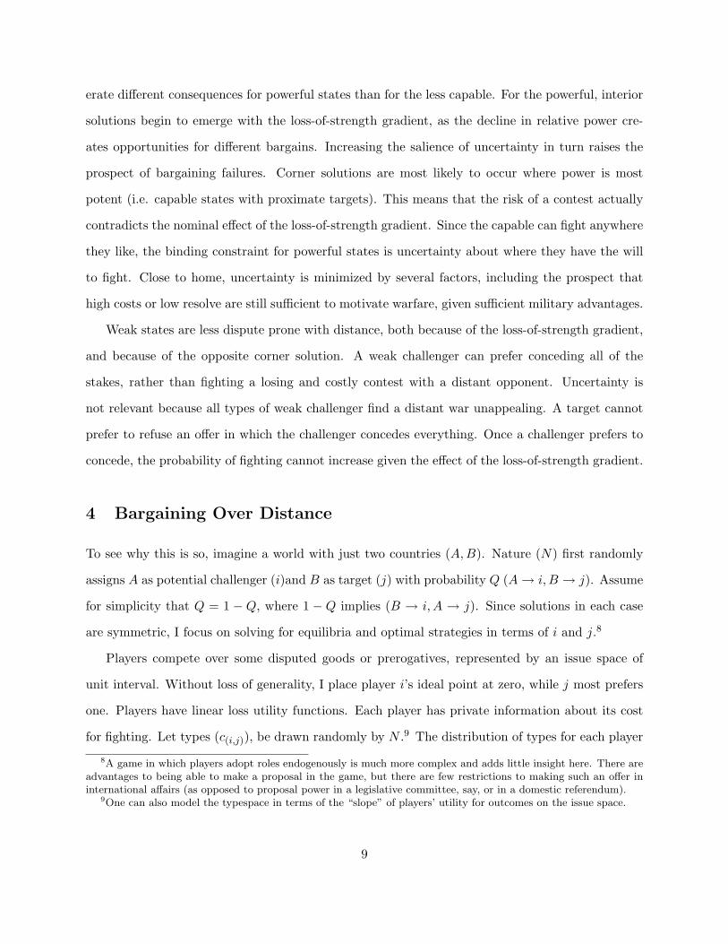
)(−a (f (1− t̄i) + t̄i) + ci (f + t̄i − f t̄i) + cj (1− 2t̄j)) (8)

For challengers with capabilities less than p̄0, the probability of a contest is declining in k. For

p0 > p̄0, Prob (war) is increasing in k. Empirically, the portion of challengers that experience a

decline in conflict with distance, and the portion that experience an increase in conflict depends on

the estimation of parameters of the model. Nevertheless, we can derive the following hypotheses.

Hypothesis 1 States are generally less likely to experience contests with increasing distance.

Hypothesis 2 Powerful states are more likely to experience contests with increasing distance.

Figure 1 plots Prob (war) in terms of p0 and k for a given set of values of relevant parameters.12

The x axis details state i’s contiguous capabilities or the probability of victory (p0). The y axis

measures distance. The maximum value of 12,500 roughly equals half the distance around the

world at the equator, measured in miles. The vertical (z) axis reports the probability of fighting

in the model. Note the complex surface created by the interaction of the three axes. Prob (war) is

increasing in distance for high values of p0 and decreasing in k for most other values of the capability

variable. State i is more likely to make an offer that j prefers to fighting if i is powerful and j is

close geographically, or if i is weak and j is distant. Both Boulding’s loss-of-strength gradient and

what I will term an “increase-in-uncertainty gradient” are supported, under different conditions.

Hypothesis 2 is a novel implication of the model and of the joining of bargaining theory with

political geography proposed here. While other research suggests that the loss-of-strength gradi-

ent may be diminished by power, time or technological innovation (Boulding 1978; Buhaug and

Gleditsch 2006), no other theory predicts increased conflict with distance for powerful states.

At the same time, the effect of capabilities or the balance of power on conflict is muddy at best.

First, as Figure 1 illustrates, Prob (war) is monotonically increasing in p for distant states due both

to the increase in uncertainty and to the fact that weak states are excluded by an inability to project12Assumed values are as follows: t̄i = t̄j = 0.001, α = 0.001, β = 0.9, a = 0.05, ci = cj = 0.2, f = 1, ti = 0.25.

13

Figure 1: Relationship between Power, Proximity, and the Probability of Conflict

power. For proximate states, on the other hand, the relationship is more convoluted. Powerful

neighbors more often get their way without fighting, while the weak seldom initiate conflicts.

The fact that weak states are unlikely to initiate contests does not mean that no disputes will

ensue. It is not practical to model the ability of the target state, j, to make endogenous counter-

demands, nor is it necessary in the framework here, where I assume that the status quo point (q)

is already at j’s ideal point. In the empirical world, the combination of the effect of distance, and

two-sided bargaining is likely to minimize the effect of power on conflict, independent of distance.13

Hypothesis 3 Powerful states are no more likely to experience contests, independent of distance.

5 Research Design: Finding power

Scholars disagree about what power is, how to measure it, how it relates to observable capabilities,

and how to compare findings from different indicators (Sullivan 1990; Geller and Singer 1998). This

level of controversy regarding the central variable in international politics is not just disconcerting,13Additional extensions of the model, including endogenizing war costs, are handled in an appendix to the paper.

14

but could also derail attempts to test theories of international conflict. However, there is much

more congruence in practice than in the surrounding scholarly rhetoric. Waltz, for example, offers

the following list of ingredients of power: “size of population and territory, resource endowment,

economic capability, military strength, political stability and competence” (Waltz 1979, page 131).

While not identical, Waltz’s list is similar to the Correlates of War (COW) Composite Indicators

of National Capabilities (CINC). I proceed acknowledging the potential limitations of my efforts.

A distinction can also be made between latent and kinetic power (Rothgeb 1993). Power

represents either the ability to influence or actual acts of influencing. These versions of power can

differ in one of two ways. First, since scholars disagree about which variables constitute the inputs

to power, particular operationalizations could bias estimates of the effects of power on conflict if in

fact omitted determinants correlate poorly with the included factors. While possible, advocates of

more inclusive conceptions of power have yet to make the case that omitting these elements biases

estimates of the relationship between power and conflict, as opposed to simply making estimates

less efficient (Nye 2004). Since the focus here is on explaining militarized force rather than more

subtle forms of influence, use of material capabilities as a measure may arguably prove sufficient.

Second, some process might intervene between nominal capabilities and national policy. This

possibility is more demanding of attention in assessing relationships between capabilities and con-

flict, especially since I propose two such processes myself. Diplomacy can short-circuit the effects

of material power on conflict. Influence also occurs if targets act in anticipation of the application

of capabilities, rather than after an actual use of force. I have incorporated this possibility into the

analysis by considering factors that might account for a failure to anticipate capabilities (and thus

that invite a use of force). More elaborate treatments of these effects awaits a theory of diplomacy.

The other intervening process proposed in this study is geography. This is explicitly integrated

into the statistical model, both directly and in its interactive effect on capabilities. While certainly

not complete, I assume that an adequate operationalization of material power as influence, rather

than simple nominal capabilities, can be had by interacting capabilities and geographic distance.

For the purposes of this study, power can be defined either as the ability to influence — either

through the use of military force, or the shadow of force — or as actual influence. While power

15

as preferences theories are ambiguous about whether capabilities equal power, or whether power is

capabilities discounted by distance, an assessment of both alternatives is on hand in this analysis.

Having dutifully discounted expectations, let me note that this study intentionally relies on

the most conventional data and estimation procedures. I use probit estimation in a sample of

wars and militarized disputes in the period 1816-2000. Analyses were conducted on both directed

and undirected dyad years. I address temporal dependence with splines and peace years (Beck,

et al. 1998), correct for clustering in dyads, and use robust standard errors to correct for spatial

dependence. Unless otherwise noted, data were obtained from EUGene (Bennett and Stam 2000).

5.1 Data

Dependent Variables: I use Zeev Maoz’s construction of dyadic militarized interstate disputes

(DYMID) as the basis for three versions of the dependent variable, with a standard dichotomous

coding of “1” for the initial year of a MID, a fatal MID (a militarized dispute involving at least

one battle-related death), or a war (at least 1000 battle deaths) in the dyad and “0” otherwise

(Gochman and Maoz 1984; Jones, et al. 1996). The Maoz data are formatted for dyadic analysis.14

In addition to conflict onset or initiation, I examine the location of a militarized dispute as

a dependent variable. To the degree that my arguments about political geography are correct,

capabilities should be a particularly potent predictor of where, as opposed to whether, nations

fight. Braithwaite (2009) identifies the latitude and longitude of each MID in the COW dataset.

Capabilities: COW offers the Composite Index of National Capabilities (CINC) based on six

components: military spending and personnel, total and urban population, and iron & steel produc-

tion and energy consumption (Singer, et al. 1972, Singer 1987). While these data are certainly not

perfect (Leng 2002), they are the most widely used quantitative measure of capabilities in interna-

tional relations (c.f. Bueno de Mesquita and Lalman 1988; Bremer 1992; Maoz and Russett 1993).

Data coverage extends from 1816 to 2000 (Correlates of War Project 2005). Controversy continues

about how best to measure power (c.f. Organski 1958; Schweller 1998), but there is no reason to

believe, ex ante, that these data are biased in favor of my hypotheses, particularly given that the14The codebook and DYMID dataset are at: http://psfaculty.ucdavis.edu/zmaoz/. I use the EUGene version.

16

data collection effort was predicated on the conviction that power was a key determinant of warfare

(Singer 1963; Wayman et al. 1983). I include each state’s CINC score and the dyadic interaction

between CINC scores, as well as interactions between CINC scores and geographic distance.

There are certainly many other ways to operationalize material power relationships. For ex-

ample, researchers often include a measure of the ratio of capabilities of the stronger state to the

weaker state in a dyad (Bremer 1992, 1993; Oneal and Russett 1997, 1999). However, such a formu-

lation assumes a particular structure to power relations. A ratio also conflates rough parity of two

weak states with that of two strong states, of critical concern for this research design (Hegre 2008).

Geographic Contiguity and Distance: States that are geographically distant are generally less

likely to fight (Bremer 1992; Maoz and Russett 1992; Buhaug and Gleditsch 2006). One of the

contentions of this study is that much of the apparent effect of capabilities on conflict is really

power mitigating distance. For this reason, I use the metric distance between national capitals.15 In

addition, I measure contiguity as the proximity of land borders and the distance separating countries

by water. Contiguity also addresses boundary effects for large states (Diehl 1985; Senese 2005).16

Military Alliances: Alliances are formal agreements intended to influence conflict behavior. The

alliance variable is dichotomous, coding the presence of a defense pact in the dyad based on the

COW alliance data (Singer and Small 1966; Small and Singer 1990; Gibler and Sarkees 2004).17

Major Power Status: Powerful countries are more active internationally, leading more often to

warfare. The major power variable is a dummy coded “1” if at least one state in a dyad is a major

power according to the COW list. Since the variable confounds some of the distinctions I make

between interests and distance, I only include major power in some of the econometric models.18

Democracy : The Polity IV project codes regime type (Jaggers and Gurr. 1995). I construct

annual democracy scores for each state as the difference between Polity’s DEMOC and AUTOC

variables, as is conventional. I adopt the method recommended in the Polity codebook (Marshall15Another approach is to use “minimum distance” between states (Gleditsch and Ward 2001). However, national

borders are in part a reflection of power relationships, and previous efforts to project power. While far from perfect,measuring distance between central locations (i.e. national capitals) is arguably a better indicator here.

16It is conventional to include both contiguity and distance in the models. Omitting contiguity never results in apositive, significant effect for either CINC variable, though occasionally, these are negative and marginally significant.

17I also examined models with a dummy for all alliance ties. This variable does not significantly alter results.18For a discussion of methodological problems with control variables, see Achen (2005); Ray (2005); Clarke (2005).

17

and Jaggers 2002, pages 15-16) for recoding cases of interregnum and transition. To compute

a dyad-level democracy score, I apply Dixon’s (1994) weak-link logic (in dyadic analysis), or the

monadic values plus an interaction term (in directed dyads), much as with the capabilities variables.

Temporal Splines: A well-established problem in Time-Series–Cross-Section Analysis (TSCS)

is the non-independence of observations. Beck et al. (1998) recommend the use of a set of lagged

dependent variables to control for temporal dependence. This approach has become the standard

in the literature. I create four “spline” variables for each of the three dependent variables.19

6 Analysis

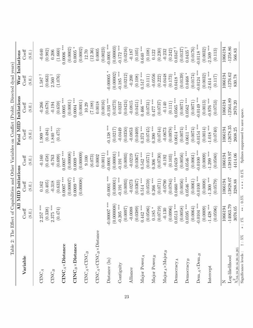
Results for the study are organized into four tables and five figures.20 The first two tables contain

seven regressions each, while the third table includes four regressions and the fourth table lists

two regressions. Table 1 reports three regressions involving “All MIDs,” two regressions of “Fatal

MIDs,” and two regressions predicting MID “Wars,” all at the dyad unit-of-analysis. Table 2

continues the analysis in a sample of directed dyads, this time focusing on “MID Initiations”,

“Fatal MID Init.” and “War Initiations.” Details of Tables 3 and 4 are discussed later in the text.

The first three regressions of “All MIDs” in Table 1 include the minimum of right-hand-side

variables, just various combinations of the CINC scores, distance, contiguity, “peaceyears” and

temporal splines (peaceyears and splines are omitted from all tables to save space). In the first

column of coefficients and standard errors, each CINC variable has a statistically significant impact

on whether states fight. The relationship is log-additive; the greater the capabilities of either

state, the more likely the dyad is to experience a MID. Contiguity and distance are also significant

predictors of conflict (higher contiguity values equal a looser definition of contiguity). Still, this

initial model specification assumes that the effect of power on conflict is independent of proximity.

The second column of coefficient estimates and standard errors in Table 1 adds interaction

terms between the two monadic CINC variables and the distance variable. This makes it possible

to differentiate the effect of power on opportunity, and on willingness (Most and Starr 1990; Siverson19Coefficients and standard errors for spline variables are not reported since they lack a substantive interpretation.20A STATA “do” file is available from the author that reproduces all aspects of data manipulation and analysis.

18

Tab

le1:

The

Effe

ctof

Cap

abili

ties

and

Oth

erV

aria

bles

onC

onfli

ct(P

robi

t,D

yad

year

s)

All

MID

sFat

alM

IDs

War

s

Var

iable

Coe

ffC

oeff

Coe

ffC

oeff

Coe

ffC

oeff

Coe

ff(S

.E.)

(S.E

.)(S

.E.)

(S.E

.)(S

.E.)

(S.E

.)(S

.E.)

CIN

CA

3.72

1∗∗∗

0.50

10.

0416

2.83

4∗∗∗

-0.1

151.

995∗∗∗

-0.6

82(0

.301

)(0

.609

)(0

.619

)(0

.481

)(0

.971

)(0

.591

)(0

.940

)C

INCB

4.44

6∗∗∗

-0.3

62-1

.322

2.28

6∗∗

-2.0

743.

045∗∗∗

-1.5

01(0

.450

)(1

.230

)(1

.013

)(0

.773

)(1

.411

)(0

.770

)(1

.320

)C

INCA×

Dis

tance

0.52

0∗∗∗

0.59

0∗∗∗

0.55

1∗∗∗

0.00

07∗∗∗

(0.0

82)

(0.0

82)

(0.1

30)

(0.0

002)

CIN

CB×

Dis

tance

0.73

1∗∗∗

0.86

4∗∗∗

0.83

3∗∗∗

0.00

1∗∗∗

(0.1

53)

(0.1

21)

(0.1

73)

(0.0

002)

CIN

CA×

CIN

CB

21.3

511

.57

30.1

437

.08†

(25.

45)

(8.2

74)

(22.

41)

(16.

63)

CIN

CA×

CIN

CB×

Dis

tanc

e-3

.153

-3.4

61-2

.627

(3.3

58)

(2.8

07)

(1.9

56)

Dis

tanc

e(l

n)-0

.165∗∗∗

-0.1

97∗∗∗

-0.1

99∗∗∗

-0.0

97∗∗∗

-0.1

32∗∗∗

-0.0

0005∗

-0.0

001∗∗∗

(0.0

06)

(0.0

06)

(0.0

06)

(0.0

16)

(0.0

16)

(0.0

0002

)(0

.000

03)

Con

tigu

ity

-0.1

17∗∗∗

-0.1

14∗∗∗

-0.1

16∗∗∗

0.67

1∗∗∗

0.64

8∗∗∗

0.93

0∗∗∗

0.85

0∗∗∗

(0.0

19)

(0.0

19)

(0.0

19)

(0.1

20)

(0.1

17)

(0.1

05)

(0.1

07)

Alli

ance

-0.1

36-0

.150†

-0.1

30-0

.118

(0.0

78)

(0.0

74)

(0.1

11)

(0.1

08)

Maj

orP

ower

0.30

9∗∗

0.48

3∗∗∗

(0.1

10)

(0.1

11)

Dem

ocra

cy(l

ow)

-0.0

59∗∗

-0.0

59∗

(0.0

19)

(0.0

20)

Dem

ocra

cy(h

igh)

0.03

2†

0.02

8(0

.015

)(0

.015

)In

terc

ept

-0.3

74∗

-0.1

97-0

.178

-2.2

77∗∗∗

-2.1

02∗∗∗

-3.3

18∗∗∗

-3.1

07∗∗∗

(0.1

30)

(0.1

23)

(0.1

23)

(0.1

60)

(0.1

61)

(0.1

33)

(0.1

45)

N65

6621

6566

2165

6621

6566

2165

6621

5330

9753

3097

Log

-lik

elih

ood

-122

79.4

45-1

2063

.424

-120

58.2

64-2

979.

710

-291

9.41

7-1

147.

074

-112

5.18

1χ

2 (9,1

1,1

3,1

1,1

4,1

3,1

7)

1572

.34

1979

.26

2271

.40

884.

3994

3.34

689.

3250

0.87

Sig

nifi

cance

level

s:†

:5%

∗:

1%

∗∗:

0.5

%∗∗∗

:0.1

%Splines

suppre

ssed

tosa

ve

space

.

19

and Starr 1990). These results suggest that the major impact of capabilities is in the ability to

overcome distance. The interaction terms between distance and CINC scores are both highly

statistically significant, while the CINC scores themselves are no longer significant. The distance

variable, however, continues to significantly influence dispute propensities, as does contiguity.

The specification in the second model in Table 1 ignores other interactions between the two

monadic capabilities variables and distance. To be thorough, interaction terms must consider all

combinations of component variables, as well as the components themselves (Braumoeller 2004).

The third and final “All MIDs” regression introduces interaction terms between the two monadic

capability variables (CINCA×CINCB) and a measure of the complex interaction between distance

and both CINC scores (CINCA×CINCB×Distance). Neither of the two additional interaction

variables is statistically significant and none of the other variables in this model is much altered

from the previous model. Only the CINC×Distance interaction variables are statistically significant.

Figure 2 plots predicted probabilities of a MID based on the third All MIDs regression in Table

1. The x axis varies state A’s capabilities, (CINCA), while the y axis lists the natural log of the

distance variable (Distance (ln)). Since it is impossible to plot relationships in more than three

dimensions, I set State B’s CINC score to the global mean (just under 1% of the world total).21

All other interval variables are held at their means, while dummy variables take modal values.

The surface representing the probability of a war is curled up at opposite ends, like a kite in a

brisk wind or a skate swimming along the bottom of the ocean. The high points, where disputes are

most likely, occur at the front and back of the image, between weak-proximate states, and between

distant states when at least one dyad member is a capable country. Proximate states experience

slightly fewer disputes as one country in the dyad becomes disproportionately powerful, but the

effect is extremely small, and apparently statistically insignificant. In contrast, distant dyads behave

in substantially different ways depending on the dyadic balance of power. As political geographers

such as Boulding predict, dyads containing two weak states are much less likely to host disputes

as distance increases. For the weak, the constraining effect of geography dominates other motives

for conflict. As at least one state in a dyad becomes highly capable, however, the decay in conflict21Other values of CINCB can be used, or State A can be the state with fixed CINC score, with equivalent results.

20

Figure 2: The Impact of Power and Proximity on War (Logit, based on Model 3, Table 1)

propensity with distance flattens out, eventually reversing. Dyads containing the most powerful

states are actually more likely to experience conflict with increasing distance. The effect of power

on dispute propensity is almost wholly intermediated through distance. Powerful states are slightly

less likely to fight their neighbors but (surprisingly) are much more likely to fight far from home.

Many of the disputes in the All MIDs sample involve relatively minor clashes. Non-fatal MIDs

arguably fall short of the dispute intensity that some theories of conflict seek to explain. To

begin to address this concern, the fourth and fifth columns list coefficient estimates and standard

errors in a sample of militarized disputes involving at least one battlefield fatality. Though it

was added to the third model in the All MIDs regressions, I include the interaction between the

capabilities of states in the dyad. Arguments about power often imply non-linear effects. It has

been claimed, for example, that rough parity is associated either with a decrease (Waltz 1959),

or an increase (Kugler and Lemke 1996) in conflict. I also add a dummy variable for alliance

status (Snyder 1997; Walt 1987). Interacting CINC scores fails to reveal a statistically significant

relationship, while monadic CINC scores are again significant, as in the first All MIDs regression.

Alliance ties are marginally statistically significant only in the second Fatal MIDs model.22 With22Leeds (2003) and Johnson and Leeds (2011) find that defensive alliances are successful in deterring aggression.

21

the interaction terms between capabilities and distance in the second Fatal MIDs regression, results

again parallel those for the all MIDs sample, with significance shifting to the interaction terms.

The last two regressions in Table 1 repeat the process of comparing the direct and indirect

effects of capabilities and distance, this time by examining MID wars. In the penultimate model

in the table, I drop the interaction term between monadic CINC scores as it was not statistically

significant. I add controls for major power status and regime type. Major power dyads are more

warlike, while democratic dyads are less inclined to experience wars. The final model in Table 1

again introduces the interaction terms between capabilities and distance. Monadic CINC scores

are again insignificant, while the joint effect of capabilities appears marginally significant at the

5% level with all interaction terms included in the MID war model. Pairs of capable states are

slightly more likely to experience wars, though the effect is modest. Finally, interactions between

capabilities and distance are again highly statistically significant, as predicted by the formal model.

Table 2 extends the analysis to directed dyads, making it possible to separate the effect of

power on potential initiators and targets. The table again lists three sets of regressions, roughly

conforming to regressions in Table 1. The first set of three regressions examines the determinants of

“MID Initiations” for all militarized disputes. In the absence of the CINC × Distance interaction

terms, capable states appear more likely to initiate disputes, and more likely to become targets of

MIDs. Introducing the interaction terms again causes the direct effects of capabilities to become

statistically insignificant. In comparing coefficients and standard errors, capabilities again influence

conflict primarily through interacting with distance. Other variables perform largely as expected.

Given complex interactions between key variables, the reported tabular results are far from

intuitive. For example, standard significance tests cannot indicate whether non-linear relationships

are statistically significant for all values of relevant variables (Braumoeller 2004). An interesting

non-linear effect could turn out to be statistically insignificant precisely whre it becomes interesting.

If the apparent increase in MID behavior with distance for powerful states is not in itself statistically

significant, this would considerably weaken the validity of my interpretation of these results.

To address this concern, and as an additional check on the results reported in Figure 2 and

the tables, I plot the predicted relationship between capabilities, distance, and militarized disputes

22

Tab

le2:

The

Effe

ctof

Cap

abili

ties

and

Oth

erV

aria

bles

onC

onfli

ct(P

robi

t,D

irec

ted

dyad

year

s)A

llM

IDIn

itia

tion

sFat

alM

IDIn

itia

tion

sW

arIn

itia

tion

sV

aria

ble

Coe

ffC

oeff

Coe

ffC

oeff

Coe

ffC

oeff

Coe

ff(S

.E.)

(S.E

.)(S

.E.)

(S.E

.)(S

.E.)

(S.E

.)(S

.E.)

CIN

CA

2.25

7∗∗∗

0.16

2-0

.160

1.90

9∗∗∗

-0.2

661.

587†

-0.6

40(0

.338

)(0

.405

)(0

.458

)(0

.484

)(0

.678

)(0

.663

)(0

.982

)C

INCB

2.37

5∗∗∗

-0.3

18-0

.763

1.84

0∗∗∗

-0.1

942.

560†

0.20

6(0

.474

)(0

.633

)(0

.699

)(0

.475

)(0

.659

)(1

.076

)(1

.660

)C

INCA×

Dis

tance

0.00

07∗∗∗

0.00

07∗∗∗

0.00

05∗∗∗

0.00

06∗∗∗

(0.0

0007

)(0

.000

08)

(0.0

001)

(0.0

002)

CIN

CB×

Dis

tance

0.00

09∗∗∗

0.00

09∗∗∗

0.00

04∗∗∗

0.00

05∗

(0.0

0008

)(0

.000

09)

(0.0

001)

(0.0

002)

CIN

CA×

CIN

CB

9.10

010

.29

12.7

0(6

.073

)(7

.188

)(1

2.36

)C

INCA×

CIN

CB×

Dis

tanc

e0.

0002

0.00

180.

0005

(0.0

011)

(0.0

016)

(0.0

023)

Dis

tanc

e(l

n)-0

.000

07∗∗∗

-0.0

001∗∗∗

-0.0

001∗∗∗

-0.1

38∗∗∗

-0.1

93∗∗∗

-0.0

0005∗

-0.0

001∗∗∗

(0.0

0000

8)(0

.000

01)

(0.0

0001

)(0

.021

7)(0

.027

3)(0

.000

02)

(0.0

0003

)C

onti

guit

y-0

.205∗∗∗

-0.1

91∗∗∗

-0.1

91∗∗∗

-0.0

449

0.02

37-0

.185∗∗∗

-0.1

72∗∗∗

(0.0

097)

(0.0

093)

(0.0

093)

(0.0

350)

(0.0

424)

(0.0

212)

(0.0

216)

Alli

ance

-0.0

088

-0.0

273

-0.0

219

-0.0

853

-0.0

815

-0.2

00-0

.187

(0.0

389)

(0.0

367)

(0.0

367)

(0.0

469)

(0.0

451)

(0.1

08)

(0.1

05)

Maj

orP

owerA

0.44

2∗∗∗

0.51

4∗∗∗

0.54

2∗∗∗

0.37

3∗∗∗

0.46

6∗∗∗

0.51

7∗∗∗

0.64

0∗∗∗

(0.0

586)

(0.0

559)

(0.0

571)

(0.0

745)

(0.0

731)

(0.1

11)

(0.1

08)

Maj

orP

owerB

0.18

5∗

0.26

6∗∗∗

0.30

6∗∗∗

0.39

0∗∗∗

0.47

7∗∗∗

-0.0

556

0.12

2(0

.071

9)(0

.071

1)(0

.073

0)(0

.074

4)(0

.073

7)(0

.222

)(0

.230

)M

ajorA×

Maj

orB

-0.1

30-0

.079

0-0

.192

-0.0

673

-0.1

40-0

.044

8-0

.232

(0.0

996)

(0.0

784)

(0.1

03)

(0.0

978)

(0.1

11)

(0.1

73)

(0.2

42)

Dem

ocra

cyA

0.05

13∗∗∗

0.04

60∗∗∗

0.04

59∗∗∗

0.06

14∗∗∗

0.05

65∗∗∗

0.04

18∗∗

0.03

47†

(0.0

058)

(0.0

056)

(0.0

056)

(0.0

074)

(0.0

071)

(0.0

139)

(0.0

137)

Dem

ocra

cyB

0.05

95∗∗∗

0.05

46∗∗∗

0.05

46∗∗∗

0.06

11∗∗∗

0.05

62∗∗∗

0.04

68∗

0.04

35†

(0.0

064)

(0.0

061)

(0.0

061)

(0.0

074)

(0.0

071)

(0.0

174)

(0.0

176)

Dem

. A×

Dem

. B-0

.010

4∗∗∗

-0.0

100∗∗∗

-0.0

100∗∗∗

-0.0

154∗∗∗

-0.0

149∗∗∗

-0.0

124∗∗∗

-0.0

118∗∗∗

(0.0

009)

(0.0

008)

(0.0

009)

(0.0

014)

(0.0

013)

(0.0

032)

(0.0

032)

Inte

rcep

t-1

.428∗∗∗

-1.3

00∗∗∗

-1.2

99∗∗∗

-1.0

18∗∗∗

-0.9

76∗∗∗

-2.6

14∗∗∗

-2.5

09∗∗∗

(0.0

596)

(0.0

579)

(0.0

580)

(0.0

740)

(0.0

753)

(0.1

17)

(0.1

13)

N10

6619

410

6619

410

6619

410

6619

410

6619

410

6619

410

6619

4L

og-l

ikel

ihoo

d-1

4063

.79

-138

28.0

7-1

3819

.97

-126

78.3

5-1

2564

.89

-127

6.62

-125

8.86

χ2 (1

6,1

8,2

0,1

6,2

0,1

6,2

0)

3076

.05

3288

.88

4414

.06

2608

.25

2870

.20

830.

7856

6.83

Sig

nifi

cance

level

s:†

:5%

∗:

1%

∗∗:

0.5

%∗∗∗

:0.1

%Splines

suppre

ssed

tosa

ve

space

.

23

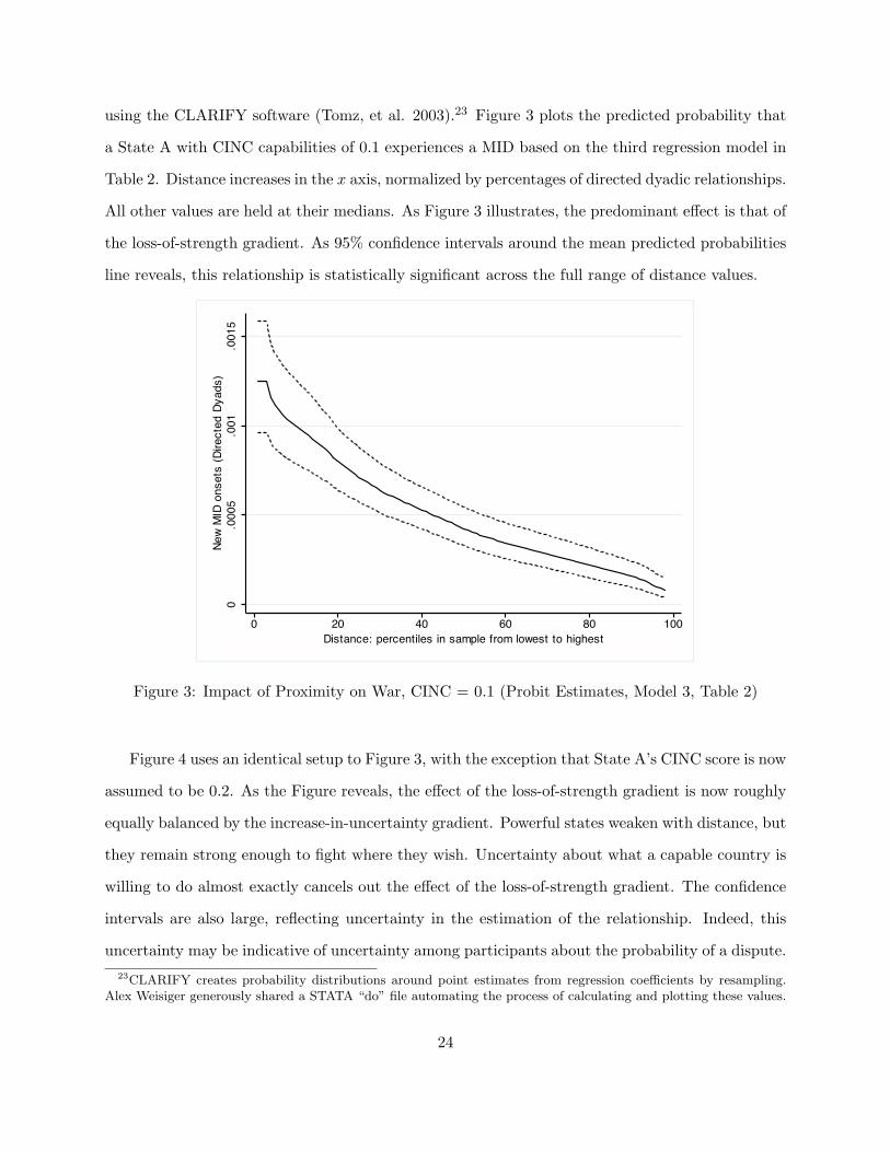
using the CLARIFY software (Tomz, et al. 2003).23 Figure 3 plots the predicted probability that

a State A with CINC capabilities of 0.1 experiences a MID based on the third regression model in

Table 2. Distance increases in the x axis, normalized by percentages of directed dyadic relationships.

All other values are held at their medians. As Figure 3 illustrates, the predominant effect is that of

the loss-of-strength gradient. As 95% confidence intervals around the mean predicted probabilities

line reveals, this relationship is statistically significant across the full range of distance values.

0.0

005

.001

.001

5Ne

w M

ID o

nset

s (D

irect

ed D

yads

)

0 20 40 60 80 100Distance: percentiles in sample from lowest to highest

Figure 3: Impact of Proximity on War, CINC = 0.1 (Probit Estimates, Model 3, Table 2)

Figure 4 uses an identical setup to Figure 3, with the exception that State A’s CINC score is now

assumed to be 0.2. As the Figure reveals, the effect of the loss-of-strength gradient is now roughly

equally balanced by the increase-in-uncertainty gradient. Powerful states weaken with distance, but

they remain strong enough to fight where they wish. Uncertainty about what a capable country is

willing to do almost exactly cancels out the effect of the loss-of-strength gradient. The confidence

intervals are also large, reflecting uncertainty in the estimation of the relationship. Indeed, this

uncertainty may be indicative of uncertainty among participants about the probability of a dispute.23CLARIFY creates probability distributions around point estimates from regression coefficients by resampling.

Alex Weisiger generously shared a STATA “do” file automating the process of calculating and plotting these values.

24

.000

5.0

01.0

015

.002

.002

5.0

03Ne

w M

ID o

nset

s (D

irect

ed D

yads

)

0 20 40 60 80 100Distance: percentiles in sample from lowest to highest

Figure 4: Impact of Proximity on War, CINC = 0.2 (Probit Estimates, Model 3, Table 2)

In Figure 5, State A’s capabilities are again increased, this time to a CINC score of 0.3. Here,

the effect of proximity has reversed itself, leading to more directed dyadic MIDs with distance.

While the most capable countries are still affected by the loss-of-strength gradient, the increase-in-

uncertainty gradient is now a more important determinant of conflict. As the confidence interval

again reveals, this relationship is statistically significant at the 95% level across the entire range

of values for the distance variable, though here again uncertainty increases with distance, possibly

reflecting the informational problem among actors that the estimation is meant to identify.

The direct effect of material power can be assessed independent of distance by holding distance

constant, and varying State A’s capabilities.24 As Figure 6 reveals, for most values of the relevant

variables, changes in State A’s power have no effect on whether A and B fight. The plot of

the effect of A’s capabilities on the probability of a MID is flat until somewhere above the 90

percentile. The fact that the estimated relationship curves upward steeply at high levels of CINCA

provides some support for the power as preferences perspective. Indeed, this evidence substantiates24Distance is set to zero, since other values allow the indirect effect of capabilities through the interaction terms.

25

0.0

1.0

2.0

3Ne

w M

ID o

nset

s (D

irect

ed D

yads

)

0 20 40 60 80 100Distance: percentiles in sample from lowest to highest

Figure 5: Impact of Proximity on War, CINC = 0.3 (Probit Estimates, Model 3, Table 2)

the assertion among realist scholars that great power conflict is distinct and worthy of separate

attention. Additional research is needed to determine whether this effect is the result of great power

competition, or whether it is produced by hegemonic policing of the international system. For now,

we can interpret these findings as showing that power relations are irrelevant for predicting conflict

in over 90% of directed dyads, once the indirect effects of capabilities on distance are addressed.

The fourth and fifth columns of estimated coefficients and standard errors in Table 2 examine

dispute initiation involving fatal MIDs, while the final paired columns predict MID war initiation.

Results for key variables are similar for all of the models.25 Introducing a measure of the interaction

between distance and capabilities causes the effect of material power on conflict to disappear.

Several interesting relationships emerge from the other independent variables. First, in most

cases major power status is a significant determinant of dispute initiation, though not for targets25In examining many combinations of models I found that the interaction terms are always statistically significant.

One or both of the monadic CINC scores can sometimes become statistically significant in certain model specifications,typically when the sample of disputes is small (i.e. MID war initiations), and when I fail to include control variables.

26

0.0

05.0

1.0

15Ne

w M

ID o

nset

s (D

irect

ed D

yads

)

0 20 40 60 80 100State A's capabilities: percentiles in sample from lowest to highest

Figure 6: Impact of Power on War, Contiguous States (Probit Estimates, Model 3, Table 2)

in MID wars.26 This finding may reflect Snyder’s (1965) stability-instability paradox.27 Opponents

are modestly deterred from initiating full-scale wars against major powers. Instead, there is an

increase in smaller-scale conflict, perhaps involving brinkmanship. Indeed, pairs of major powers

are less likely to experience MIDs, though the relationship is not statistically significant. Relations

among major powers appear no more dispute prone. Instead, most of the impact of major power

status occurs in relation to non-major powers. Finally, the effects of regime type appear to vary

with conflict intensity. The dyadic democratic peace is best reflected in the MID wars sample. The

dyadic relationship is contrasted with monadic increases in conflict at lower dispute intensities.

Proximity seems to matter most in determining the impact of capabilities. Still, countries could

fight in places distant or distinct from the homeland, and the most powerful nations are the most

likely to relocate their contests. Since disputes can occur far from any participant, a different

and arguably more precise test of the claim that power conditions distance can be had by looking

at the location of disputes. Data from (Braithwaite 2010) identifies the location of each MID.26Coding of major power status by COW is subjective and reflects capabilities and involvement in interstate politics.27For a recent study documenting the stability-instability paradox in nuclear weapons, see Rauchhaus (2009).

27

Additional work by Braithwaite and this author produced a dataset of distances from the latitude

and longitude of every MID to the capital cities of each dispute participant. Since these data select

on the dependent variable (how does one assign a location to a non-dispute?), it is not possible to

evaluate the MID location data in the same manner as when studying dispute onset or initiation.

I adopt two approaches to assess the impact of capabilities and other variables on dispute location.

First, I examine the determinants of location in the sample of disputes. Next, using two-stage

regression, I first estimate the probability of a MID, and then model the resulting conflict location.

Table 3 provides four regressions in which capabilities, dyadic distance and other variables pre-

dict the distance from the capital of the initiating country to the location of the militarized dispute.

Ordinary Least Squares (OLS) is used, since the dependent variable is metric and continuous. The

first regression is “monadic” as only the CINC score of the initiating state and monadic control

variables are included in the regression. The more capable the country initiating a contest, the

more distant is the dispute from the capital of the initiating nation. Having more neighbors tends

to cause a country to fight closer to home, while increasing the sample of countries in the world

causes contests to occur farther from the initiator’s capital (probably an artifact of how colonial

dependencies are coded in the COW data). The number of countries variable helps to ensure that

the analysis is not driven by evolving national boundaries. The number of great powers appears to

decrease the distance to disputes, but as we shall see, this result is really an artifact of time.

The second regression in Table 3 introduces “dyadic” variables, though the model is again

minimalist to show that relationships are not contingent on model specification (Ray 2005; Clarke

2005). While the capabilities of the initiator continues to significantly increase the distance between

the initiator’s capital and the location of the dispute, the CINC score of the target does the opposite.

Capable targets tend to force initiators to fight closer to the initiator’s home, constraining where

initiators fight, a “balance of location,” rather than a balance of power effect. The interaction

between capabilities is not statistically significant. The location of contests is determined by a

tug-o-war between the capabilities of disputants, not by the relative power of the two nations.

The second regression adds a conventional dyadic distance variable. The variable shows that

the relationship between capabilities and distance-to-dispute is not just a by-product of correla-

28

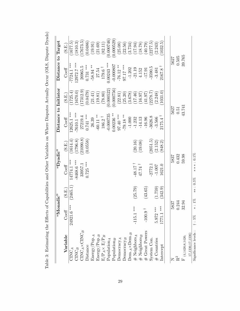
Tab

le3:

Est

imat

ing

the

Effe

cts

ofC

apab

iliti

esan

dO

ther

Var

iabl

eson

Whe

reD

ispu

tes

Act

ually

Occ

ur(O

LS,

Dis

pute

Dya

ds)

“M

onad

ic”

“D

yadic

”D

ista

nce

toIn

itia

tor

Dis

tance

toTar

get

Var

iable

Coe

ff(S

.E.)

Coe

ff(S

.E.)

Coe

ff(S

.E.)

Coe

ff(S

.E.)

CIN

CA

2492

1.6∗∗∗

(246

5.1)

1477

4.1∗∗∗

(161

4.4)

1262

5.1∗∗∗

(172

5.4)

-772

4.1∗∗∗

(167

7.5)

CIN

CB

-846

8.6∗∗∗

(179

6.8)

-761

0.1∗∗∗

(167

0.0)

1297

2.7∗∗∗

(181

0.3)

CIN

CA×

CIN

CB

3395

7.1

(210

90.8

)27

219.

4(1

7312

.9)

2696

5.5

(176

73.5

)D

ista

nce

0.72

5∗∗∗

(0.0

558)

0.74

1∗∗∗

(0.0

479)

0.73

1∗∗∗

(0.0

486)

Ene

rgy/

Pop

. A26

.39

(21.

41)

-58.

94∗∗

(19.

91)

Ene

rgy/

Pop

. B-6

0.11∗∗

(19.

81)

27.5

4(2

1.69

)E

/PA×

E/P

B18

6.2†

(78.

80)

179.

6†

(82.

11)

Pop

ulat

ion A

-0.0

0073

5(0

.000

522)

0.00

243∗∗∗

(0.0

0074

6)P

opul

atio

n B0.

0023

6∗∗

(0.0

0075

6)-0

.000

807

(0.0

0052

9)D

emoc

racyA

97.4

0∗∗∗

(22.

81)

-76.

12∗∗

(25.

08)

Dem

ocra

cyB

-79.

18∗∗

(25.

20)

97.1

7∗∗∗

(22.

56)

Dem

. A×

Dem

. B-1

.000

(3.6

78)

-1.2

02(3

.734

)#

Nei

ghbo

rsA

-115

.1∗∗∗

(25.

79)

-48.

17†

(20.

16)

-1.2

32(1

7.46

)-2

1.19

(17.

94)

#N

eigh

borsB

47.7

4†

(19.

08)

-14.

13(1

6.97

)4.

152

(18.

78)

#G

reat

Pow

ers

-100

.9†

(43.

65)

-16.

96(4

1.97

)-1

7.91

(40.

79)

Syst

emC

on.

-277

2.1

(205

1.5)

-362

6.8

(227

8.7)

-359

0.5

(227

7.5)

#C

ount

ries

5.97

2∗∗∗

(1.7

59)

-1.0

07(2

.152

)-3

.566

(2.2

48)

-3.4

81(2

.243

)In

terc

ept

1771

.1∗∗∗

(342

.9)

1621

.0(8

48.2

)21

75.4†

(103

1.0)

2167

.8†

(103

2.5)

N58

3758

3756

2756

27R

20.

244

0.43

20.

510.

505

F(4,1

426;8,1

426;

32.9

459

.98

43.7

4139

.765

17,1

336;1

7,1

336)

Sig

nifi

cance

level

s:†

:5%

∗:

1%

∗∗:

0.5

%∗∗∗

:0.1

%

29

tion between power and proximity. Powerful states could cluster closer together (Gleditsch 2003).

Alternately, powerful states could cause neighbors to become weaker, endogenously generating a

correlation between capabilities and distance. Whatever the relationship, it does not appear to con-

found the analysis. The distance between capital and conflict increases with the distance between

states, but the effect of power on distance remains statistically significant. The respective effects of

the # Neighbors variables are also informative. While having more neighbors forces an initiator to

stay closer to home in fighting a given opponent, it does the opposite for a target. Neighbors make

a target more vulnerable to contagion effects or side-disputes, allowing the initiator to be bolder in

incurring on the target’s territory. While not significant, I replace the # of Great Powers variable

with the COW System Con. variable, which measures the concentration of global capabilities.

The third regression in Table 3 introduces variables to address heterogeneity in development,

population and regime type. Tremendous changes in the last century risk generating a spurious

correlation between power and proximity. Economic development has increased exponentially.

Advances in technology diminish the impact of distance, even as they alter priorities (Buhaug and

Gleditsch 2006). Average national population has grown from roughly 10 million before 1850, to

more than 32 million today. Research also emphasizes differences in democratic foreign policy

(Doyle 1986; Owen 1997; Russett and Oneal 2001). While these variables do matter, they do not

appear to alter the impact of power on location in a fundamental way. Capable initiators still fight

farther from home, while powerful targets force fighting to occur closer to the initiator’s capital.

Energy consumption per capita correlates closely with economic development, but allows the

analysis to extend well into the 19th century. Intensive energy consumption by initiators does not

significantly affect the location of contests, but initiators fight closer to home when the target is a

developed state. The population size of initiating countries does not much matter for the location

of militarized contests, but populous targets tend to encourage the initiator to fight a bit farther

from home. Perhaps because they desire to secure domestic populations from harm, democratic

initiators and targets tend to fight at greater distances from the homeland. Again, this may reflect

a “not in my back yard” bias attributable to popular rule. Other variables perform as expected.

The fourth regression in Table 3 uses distance from the target state to the MID as an additional

30

test of the effects of power on the proximity of contests. All independent variables are as in the

previous regression model. If power is conditioning distance, then we should expect the two monadic

capability variables to swap signs and coefficient magnitudes, while most other variables remain

unaffected. This is exactly what we observe. The CINC score of the initiator now decreases the

distance between a dispute and the target’s capital, while a capable target forces the fight to occur

farther from the target’s home. The monadic development, population, and regime type variables

also change signs, magnitudes and statistical significance levels, indicating that the distance to

dispute dependent variable is probably capturing distance and not another process (such as time).

An important source of concern involves selection. An assessment of the location of contests may

bias estimates if the determinants of dispute distance are related to the determinants of disputes.

Obviously, many of the variables used in Table 3 are similar or identical to those used in Tables

1 and 2. Heckman (1978) offers the classic exposition of a solution to this problem in the form of

two-stage regression. Heckman’s two-stage estimator first models the biasing effect of participation,

and then corrects for this bias in estimating within-sample differentials. In estimating differences in

location between weak and capable states, one must correct for any disparity in the propensity of

weak and capable countries to experience disputes. If less capable states experience less (or more)

conflict, then this will tend to underestimate (or overestimate) the effect of capabilities on location.

Not coincidentally, the dispute onset stage estimation is also a useful test of the hypotheses.

Table 4 lists two two-stage Heckman regressions, in which the first stage (selection equation)

estimates the probability of MID onset, and the second stage (outcome equation) predicts the

location of disputes. These regressions repeat the format of the third and fourth regressions in

Table 3, with the first set of coefficients and standard errors predicting the distance from the capital

of the initiator to the location of the dispute and the second set of coefficients and standard errors

modeling dispute locations relative to the target. As these results make clear, selection bias is not

interfering with the results in Table 3. The size and significance levels of coefficients in the outcome

equation are essentially unchanged. Nor is Heckman’s selection statistic (ρ) significantly different

from zero. Equally salient, CINC scores in the selection equation are statistically insignificant;

capable nations are not more likely to fight. Instead, distance continues to interact with capabilities

31

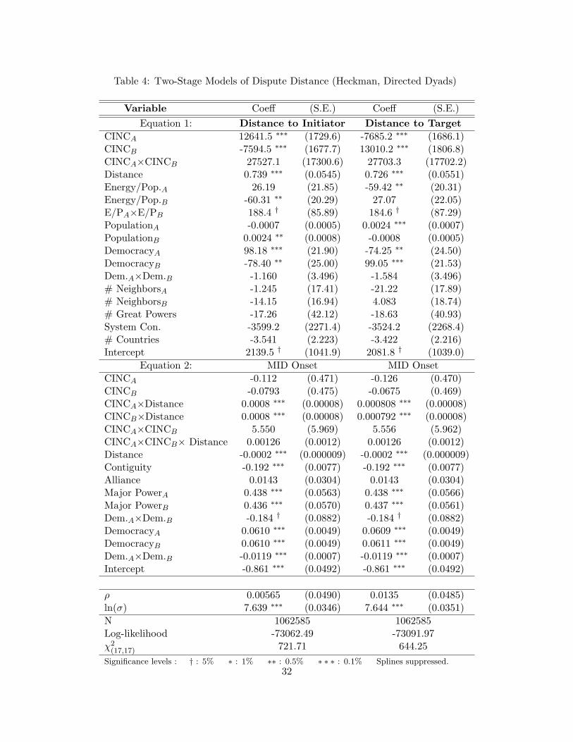
Table 4: Two-Stage Models of Dispute Distance (Heckman, Directed Dyads)

Variable Coeff (S.E.) Coeff (S.E.)Equation 1: Distance to Initiator Distance to Target

CINCA 12641.5 ∗∗∗ (1729.6) -7685.2 ∗∗∗ (1686.1)CINCB -7594.5 ∗∗∗ (1677.7) 13010.2 ∗∗∗ (1806.8)CINCA×CINCB 27527.1 (17300.6) 27703.3 (17702.2)Distance 0.739 ∗∗∗ (0.0545) 0.726 ∗∗∗ (0.0551)Energy/Pop.A 26.19 (21.85) -59.42 ∗∗ (20.31)Energy/Pop.B -60.31 ∗∗ (20.29) 27.07 (22.05)E/PA×E/PB 188.4 † (85.89) 184.6 † (87.29)PopulationA -0.0007 (0.0005) 0.0024 ∗∗∗ (0.0007)PopulationB 0.0024 ∗∗ (0.0008) -0.0008 (0.0005)DemocracyA 98.18 ∗∗∗ (21.90) -74.25 ∗∗ (24.50)DemocracyB -78.40 ∗∗ (25.00) 99.05 ∗∗∗ (21.53)Dem.A×Dem.B -1.160 (3.496) -1.584 (3.496)# NeighborsA -1.245 (17.41) -21.22 (17.89)# NeighborsB -14.15 (16.94) 4.083 (18.74)# Great Powers -17.26 (42.12) -18.63 (40.93)System Con. -3599.2 (2271.4) -3524.2 (2268.4)# Countries -3.541 (2.223) -3.422 (2.216)Intercept 2139.5 † (1041.9) 2081.8 † (1039.0)

Equation 2: MID Onset MID OnsetCINCA -0.112 (0.471) -0.126 (0.470)CINCB -0.0793 (0.475) -0.0675 (0.469)CINCA×Distance 0.0008 ∗∗∗ (0.00008) 0.000808 ∗∗∗ (0.00008)CINCB×Distance 0.0008 ∗∗∗ (0.00008) 0.000792 ∗∗∗ (0.00008)CINCA×CINCB 5.550 (5.969) 5.556 (5.962)CINCA×CINCB× Distance 0.00126 (0.0012) 0.00126 (0.0012)Distance -0.0002 ∗∗∗ (0.000009) -0.0002 ∗∗∗ (0.000009)Contiguity -0.192 ∗∗∗ (0.0077) -0.192 ∗∗∗ (0.0077)Alliance 0.0143 (0.0304) 0.0143 (0.0304)Major PowerA 0.438 ∗∗∗ (0.0563) 0.438 ∗∗∗ (0.0566)Major PowerB 0.436 ∗∗∗ (0.0570) 0.437 ∗∗∗ (0.0561)Dem.A×Dem.B -0.184 † (0.0882) -0.184 † (0.0882)DemocracyA 0.0610 ∗∗∗ (0.0049) 0.0609 ∗∗∗ (0.0049)DemocracyB 0.0610 ∗∗∗ (0.0049) 0.0611 ∗∗∗ (0.0049)Dem.A×Dem.B -0.0119 ∗∗∗ (0.0007) -0.0119 ∗∗∗ (0.0007)Intercept -0.861 ∗∗∗ (0.0492) -0.861 ∗∗∗ (0.0492)

ρ 0.00565 (0.0490) 0.0135 (0.0485)ln(σ) 7.639 ∗∗∗ (0.0346) 7.644 ∗∗∗ (0.0351)N 1062585 1062585Log-likelihood -73062.49 -73091.97χ2

(17,17) 721.71 644.25Significance levels : † : 5% ∗ : 1% ∗∗ : 0.5% ∗ ∗ ∗ : 0.1% Splines suppressed.

32

in the selection stage. Powerful countries are more likely to fight if the dispute occurs far from

home, while weak nations are slightly more dispute prone when contests are more proximate.

7 Conclusion

This study attempts to identify some scope and scale conditions for bargaining theories of war

by comparing three approaches to “rationalist” interstate conflict. While the propensity to fight

usually decays with distance, the effects of this decay first diminish and then are reversed with

rising capabilities. The weak and distant are at peace, if only out of necessity. The proximate

and powerful can fight, but may or may not need war to exact concessions from opponents. While

Boulding’s insight about the loss-of-strength gradient is generally correct, capable countries exhibit

a “gain of uncertainty gradient,” becoming more disputatious with targets that are far from home.

Each perspective on capabilities and conflict offers insights that are partial and incomplete.

Treating capabilities as preferences is perhaps least sustainable, though the approach may be de-

fensible in the context of great powers, as realists have long argued. For the vast majority of

interactions in international affairs, the juxtaposition of capabilities is relatively impotent as an

explanation for interstate conflict. Indeed, future research may focus with additional confidence

on the atypical role of great powers. However, it remains to be shown whether power itself is the

cause of this divergence or whether it is the result of other factors, such as leadership or hegemony.

The most important events in international politics may indeed be explained by differences in

the capabilities of nations, but rationalizing this claim may well require researchers to focus on what

is important to practitioners, rather than academics. Nations in competition seek to redistribute

benefits and prerogatives. Power relations fundamentally affect the division of global resources and

national prerogatives, but whether this results in warfare really depends on other factors. The

boundaries on spheres of influence may move much more than the nominal probability of fighting.

The powerful are not challenged close to home. Disputes begin when, and more importantly where,

influence is uncertain or control disputed. To paraphrase Mearsheimer, the locations of contests

are mainly a function of the balance of power, though the causes of war and peace lie elsewhere.

Distance is something that nations cannot dispel through diplomacy. Proximate adversaries

33

would be better off if they could agree to separate, like an estranged couple with a restraining

order. Unfortunately, space on this little planet is limited, with most locations already under

different management. Making conflict more costly by increasing the distance between countries

is impractical.28 Instead, nations seek to impose weakness through other means, like arms control

treaties or third-party guarantees. These efforts are flawed, since it is difficult to contract to impair

both parties equally, and since competitors have incentives to cheat. The weakness imposed by

distance also has the advantage of being symmetric, impairing both sides in a potential dispute.

If geography helps by imparting context to bargaining theory, improving the empirical fit, bar-

gaining theory resolves the empirical anomaly identified here, that capable states appear to cancel

and even contradict the loss-of-strength gradient. Boulding still assumed that capabilities cause

conflicts. If, as Fearon suggests, war is more a product of error than power, then the increase in

distant disputes among the capable reflects geographically-induced uncertainty. Nations capable of

projecting power make conflict possible with more counterparts. Uncertainty about whether the

powerful will resort to force increases the risk of violence because possibilities can be underesti-

mated. Increasing the ability to project power increases uncertainty about where and when power

will be projected, raising the prospects of bargaining failure, and war. The tendency of power-

ful nations to reverse the effect of the loss-of-strength gradient reflects growing uncertainty with

distance about what powerful states prefer, given many possibilities and the temptation to bluff.

28Occasionally, this is precisely what is attempted, with the creation of “weapons free” and “buffer” zones.

34

Appendix A: Endogenizing the Effect of Distance on War Costs

One of the weaknesses of the model (and indeed most other formal models of conflict) is the implau-

sible assumption that war costs are uncorrelated with other parameters, such as the probability of

victory, or an actor’s resolve. Actors are bound to be more willing or able to incur costs if they are

rich/powerful, or if they have a high value for the stakes. It is conceivable that endogenizing war

costs could lead to different predictions. However, H1-3 still hold, as I briefly demonstrate below.

Begin with Eqs 1-3. In addition, let us imagine that i’s war costs originate from some function:

ci = gi + ρi (1− p0) + γ ∗ kφ (A1)

where g is some non-negative constant such as “fighting spirit,” (1− p0) is the probability that

j wins if i is contiguous, k is the distance variable, and ρ, γ and φ are all non-negative parameters.

By analogy, j’s war costs, where the loss-of-strength for the target is zero, are as follows:

cj = gj + ρjp0 (A2)

Substituting Eqs 1, A1, and A2 into Eq 2 and 3, and solving the model as outlined in the text

yields relationships for Prob (war) and p̄0 equivalent to those generated previously. In fact, because

ci is now increasing in k, the effects of distance in decreasing conflicts involving weak attackers (i.e.

loss-of-strength) and increasing corner solutions for the strong (increase-in-uncertainty) is enhanced.

As Figure A1 illustrates, endogenizing war costs leads to relationships that are somewhat “steeper”

than in Figure 1 in the text, but the overall comparative statics remain substantively unchanged.

Appendix B: Varying the Effect of the Loss-of-Strength with Power

The impact of the loss-of-strength gradient (LSG) might vary with capabilities. Stronger states

could experience less (or more) than proportional effects of the LSG. Eq 1 is generalized as follows:

p =p0

1 + α (θkβ + (1− θ) kβ (1− p0))(A3)

35

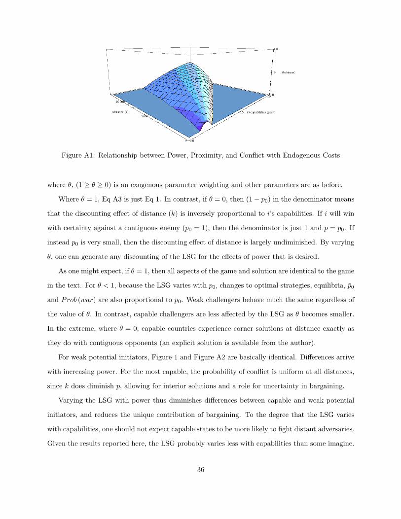
Figure A1: Relationship between Power, Proximity, and Conflict with Endogenous Costs

where θ, (1 ≥ θ ≥ 0) is an exogenous parameter weighting and other parameters are as before.

Where θ = 1, Eq A3 is just Eq 1. In contrast, if θ = 0, then (1− p0) in the denominator means

that the discounting effect of distance (k) is inversely proportional to i’s capabilities. If i will win

with certainty against a contiguous enemy (p0 = 1), then the denominator is just 1 and p = p0. If

instead p0 is very small, then the discounting effect of distance is largely undiminished. By varying

θ, one can generate any discounting of the LSG for the effects of power that is desired.

As one might expect, if θ = 1, then all aspects of the game and solution are identical to the game

in the text. For θ < 1, because the LSG varies with p0, changes to optimal strategies, equilibria, p̄0

and Prob (war) are also proportional to p0. Weak challengers behave much the same regardless of

the value of θ. In contrast, capable challengers are less affected by the LSG as θ becomes smaller.

In the extreme, where θ = 0, capable countries experience corner solutions at distance exactly as

they do with contiguous opponents (an explicit solution is available from the author).

For weak potential initiators, Figure 1 and Figure A2 are basically identical. Differences arrive

with increasing power. For the most capable, the probability of conflict is uniform at all distances,

since k does diminish p, allowing for interior solutions and a role for uncertainty in bargaining.

Varying the LSG with power thus diminishes differences between capable and weak potential

initiators, and reduces the unique contribution of bargaining. To the degree that the LSG varies

with capabilities, one should not expect capable states to be more likely to fight distant adversaries.

Given the results reported here, the LSG probably varies less with capabilities than some imagine.

36

Figure A2: Relationship between Power, Proximity, and Conflict with Endogenous Costs

Appendix C: Alternatives to the Use of Corner Solutions

There are at least two other ways to generate an increase in conflict correlated with distance for

powerful states (but not for the weak). For brevity, I offer only a sketch of the arguments here.

First, since capable countries can project power farther than weak states, the number of coun-

tries with which they can interact is naturally much larger. Yet, if countries still face opportunity

costs in the exercise of military violence, then force used against one state cannot be exercised

simultaneously against other nations. Capable countries must choose more selectively than weak

states from a larger number of potential targets. At the same time, all countries desire to obtain

preferred outcomes. This means that capable states have more incentives to bluff when dealing with

the larger number of distant states. Distant adversaries must rationally infer that the probability

of attack is lower with distance, and thus they are more likely to (incorrectly) reject i’s demands.

Second, interest may decline in distance. Even with no LSG, powerful states are less likely to

generate corner solutions if distance reduces resolve. The effect is then much the same as the model

in the text. Capable countries generate corner solutions with neighbors, while interior solutions are

produced in interactions with distant states. Weak countries, that must search for interior solutions

even with neighbors, find that the loss of value for distant issues and territory leads to the opposite

corner solution, where the weak state prefers conceding everything rather than risk fighting.

37

References

Achen, Christopher H. 2005. “Let’s Put Garbage-Can Regressions and Garbage-Can Probits Where TheyBelong.” Conflict Management and Peace Science 22(4):327–339.

Axelrod, Robert. 1984. The Evolution of Cooperation. New York: Basic Books.

Barnett, Michael and Raymond Duvall. 2005. “Power in International Politics.” International Organization59(1):39–75.

Beck, Neal, Jonathan Katz and Richard Tucker. 1998. “Taking Time Seriously: Time-series–Cross-sectionAnalysis with a Binary Dependent Variable.” American Journal of Political Science 42(4):1260–1288.

Bennett, D. Scott and Allan C. Stam. 2000. “EUGene: A Conceptual Manual.” International Interactions26(2):179–204.

Bennett, D. Scott and Allan C. Stam. 2001. “EUGene: Expected Utility and Data Management Program,version 2.250.” Computer Program. The Pennsylvania State University and Dartmouth University.

Blainey, Geoffrey. 1973. The Causes of War. New York: Free Press.

Boulding, Kenneth. 1962. Conflict and Defense. New York: Harper & Row.

Boulding, Kenneth. 1978. Stable Peace. Austin, TX: University of Texas Press.

Braithwaite, Alex. 2009. “Codebook for the Militarized Interstate Dispute Location (MIDLOC) Data, v1.0.” University College London.

Braithwaite, Alex. 2010. “MIDLOC: Introducing the Militarized Interstate Dispute Location Dataset.”Journal of Peace Research 47(1):91–98.

Braumoeller, Bear. 2004. “Hypothesis Testing and Multiplicative Interaction Terms.” International Organi-zation 58(4):807–820.

Bremer, Stuart. 1992. “Dangerous Dyads: Conditions Affecting the Likelihood of Interstate War.” Journalof Conflict Resolution 36(2):309–341.

Bremer, Stuart. 1993. “Democracy and Militarized Interstate Conflict, 1816–1965.” International Interac-tions 18(3):231–249.

Bueno de Mesquita, Bruce. 1981. The War Trap. New Haven: Yale University Press.

Bueno de Mesquita, Bruce. 2003. Neorealism’s Logic and Evidence: When is a Theory Falsified? In Realismand the Balancing of Power: A New Debate, ed. Colin Elman and John Vasquez. Englewood Cliffs, NJ:Prentice Hall pp. 166–197.

Bueno de Mesquita, Bruce and David Lalman. 1988. “Empirical Support for Systemic and Dyadic Explana-tions of International Conflict.” World Politics 41(1):1–20.

Bueno de Mesquita, Bruce and David Lalman. 1992. War and Reason: Domestic and International Imper-atives. New Haven: Yale University Press.

Buhaug, Halvard and Nils Petter Gleditsch. 2006. The Death of Distance?: The Globalization of ArmedConflict. In Territoriality and Conflict in an Era of Globalization, ed. Miles Kahler and Barbara Walter.Cambridge: Cambridge University Press.

Clarke, Kevin A. 2001. “Testing Nonnested Models of International Relations: Reevaluating Realism.”American Journal of Political Science 45(3):724–744.

Clarke, Kevin A. 2005. “The Phantom Menace: Omitted Variable Bias in Econometric Research.” ConflictManagement and Peace Science 22(4):341–352.

38

Correlates of War Project. 2005. “National Material Capabilities Data Documentation, version 3.0.” url:http://cow2.la.psu.edu/.

Deutsch, Karl W. and J. David Singer. 1964. “Multipolar Power Systems and International Stability.” WorldPolitics 16:390–406.

Diehl, Paul. 1985. “Contiguity and Military Escalation in Major Power Rivalries, 1816–1980.” Journal ofPolitics 47(4):1203–1211.

Dixon, William J. 1994. “Democracy and the Peaceful Settlement of International Conflict.” AmericanPolitical Science Review 88(2):14–32.

Downes, Alexander B. and Todd S. Sechser. 2010. “Are You Threatening Me?: A Reassessment of theCredibility of Democratic Threats in International Relations.” Paper presented at the Annual Meetingsof the American Political Science Association, Washington D.C., September 2-5.

Doyle, Michael. 1986. “Liberalism and World Politics.” American Political Science Review 80(4):1151–1169.

Fearon, James D. 1994. “Signaling Versus the Balance of Power and Interests: An Empirical Test of theCrisis Bargaining Model.” Journal of Conflict Resolution 38(2):236–269.

Fearon, James D. 1995. “Rationalist Explanations for War.” International Organization 49(3):379–414.

Filson, Darren and Suzanne Werner. 2002. “A Bargaining Model of War and Peace: Anticipating the Onset,Duration, and Outcome of War.” American Journal of Political Science 46(4):819–837.

Filson, Darren and Suzanne Werner. 2004. “Bargaining and Fighting: The Impact of Regime Type on WarOnset, Duration, and Outcomes.” American Journal of Political Science 48(2):296–313.

Gartzke, Erik and Dong-Joon Jo. 2009. “Bargaining, Nuclear Proliferation, and Interstate Disputes.” Journalof Conflict Resolution 53(2):209–233.

Geller, Daniel S. and J. David Singer. 1998. Nations at War: A Scientific Study of International Conflict.Cambridge: Cambridge University Press.

Gibler, Douglas and Meredith Reid Sarkees. 2004. “Measuring Alliances: The Correlates of War FormalInterstate Alliance Dataset, 1816–2000.” Journal of Peace Research 41(2):211–222.

Gilpin, Robert. 1981. War and Change in World Politics. New York: Cambridge University Press.

Gleditsch, Kristian S. 2003. All International Politics is Local: The Diffusion of Conflict, Integration, andDemocratization. Ann Arbor, MI: University of Michigan Press.

Gleditsch, Kristian S. and Michael D. Ward. 2001. “Measuring Space: A Minimum Distance Data Set.”Journal of Peace Research 38(4):749–768.

Gochman, Charles S. and Zeev Maoz. 1984. “Militarized Interstate Disputes, 1816-1976: Procedure, Patterns,and Insights.” Journal of Conflict Resolution 28(4):585–615.

Heckman, James J. 1978. “Sample Selection Bias as a Specification Error.” Econometrica 47(1):153–162.

Hegre, H̊avard. 2008. “Gravitating Toward War: Preponderance May Pacify, but Power Kills.” Journal ofConflict Resolution 52(4):566–589.

Huth, Paul K., Christopher Gelpi and D. Scott Bennett. 1993. “The Escalation of Great Power MilitarizedDisputes: Testing Rational Deterrence Theory and Structural Realism.” American Political ScienceReview 87(3):609–623.

Jaggers, Keith and Ted R. Gurr. 1995. “Transitions to Democracy: Tracking Democracy’s ‘Third Wave’with the Polity III Data.” Journal of Peace Research 32(4):469–482.

Johnson, Jesse C. and Brett Ashley Leeds. 2011. “Defense Pacts: A Prescription for Peace.” Foreign PolicyAnalysis 7(1):45–65.

39

Jones, Daniel, Stuart Bremer and J. David Singer. 1996. “Militarized Interstate Disputes, 1816-1992: Ratio-nale, Coding Rules, and Empirical Patterns.” Conflict Management and Peace Science 15(2):163–213.

Keohane, Robert O. 1998. “International Institutions: Can Interdependence Work?” Foreign Policy 110:82–96.

Keohane, Robert O., ed. 1986. Neorealism and its Critics. New York: Columbia University Press.

Kugler, Jacek and Douglas Lemke. 1996. Parity and War: Evaluations and Extensions of ‘The War Ledger’.Ann Arbor, MI: University of Michigan Press.

Leeds, Brett Ashley. 2003. “Do Alliances Deter Aggression?: The Influence of Military Alliances on theInitiation of Militarized Interstate Disputes.” American Journal of Political Science 47(3):427–439.

Lemke, Douglas and Suzanne Werner. 1996. “Power Parity, Commitment to Change, and War.” InternationalStudies Quarterly 40(2):235–260.

Leng, Russell J. 2002. Quantitative International Politics and Its Critics. In Millenial Reflections on Inter-national Studies, ed. Michael Brecher and Frank P. Harvey. University of Michigan Press pp. 420–431.

Mackinder, Halford. 1962[1919]. Democratic Ideals and Reality. Westport, CT: Greenwood.

Mahan, A.T. 1915. The Interest of America in International Conditions. Boston: Little, Brown, and Co.

Mahan, A.T. 1987[1890]. The Influence of Sea Power on History, 1660–1783. Fifth ed. New York: Dover.

Mansfield, Edward. 1992. “The Concentration of Capabilities and the Onset of War.” Journal of ConflictResolution 36(1):3–24.

Maoz, Zeev and Bruce Russett. 1992. “Alliances, Contiguity, Distance, Wealth, and Political Stability: Is theLack of Conflict Among Democracies a Statistical Artifact?” International Interactions 17(3):245–268.

Maoz, Zeev and Bruce Russett. 1993. “Normative and Structural Causes of the Democratic Peace, 1946-1986.” American Political Science Review 87(3):624–638.

Marshall, Monty and Keith Jaggers. 2002. “Polity IV Project: Political Regime Characteristics and Transi-tions, 1800-2002.” url: http://www.systemicpeace.org/polity/polity4.htm.

Moravcsik, John A. 1997. “Taking Preferences Seriously: A Liberal Theory of International Politics.”International Organization 51(4):515–553.

Morrow, James D. 1989. “Capabilities, Uncertainty, and Resolve: A Limited Information Model of CrisisBargaining.” American Journal of Political Science 33(2):941–972.

Most, Benjamin A. and Harvey Starr. 1990. “Opportunity, Willingness, and the Diffusion of War.” AmericanPolitical Science Review 84(1):47–67.

Moul, William. 2003. “Power Parity, Preponderance, and War between Great Powers, 1816–1989.” Journalof Conflict Resolution 47(4):468–489.

Niou, Emerson S. and Peter Ordeshook. 1986. “A Theory of the Balance of Power.” Journal of ConflictResolution 30(4):685–715.

Niou, Emerson S. and Peter Ordeshook. 1994. “Less Filling, Tastes Great: The Realist-Neoliberal Debate.”World Politics 46(2):209–234.

Niou, Emerson S., Peter Ordeshook and Gregory Rose. 1989. The Balance of Power: Stability in InternationalSystems. Cambridge: Cambridge University Press.

Nye, Joseph S. 2004. Soft Power: The Means to Success in World Politics. New York: Public Affairs.

Oneal, John R. and Bruce Russett. 1997. “The Classical Liberals Were Right: Democracy, Interdependence,and Conflict, 1950-1985.” International Studies Quarterly 41(2):267–293.

40

Oneal, John R. and Bruce Russett. 1999. “The Kantian Peace: The Pacific Benefits of Democracy, Interde-pendence, and International Organizations.” World Politics 52(1):1–37.

Oneal, John R., Bruce Russett and Michael L. Berbaum. 2003. “Causes of Peace: Democracy, Interdepen-dence, and International Organizations.” International Studies Quarterly 47(3):371–393.

Organski, A.F.K. 1958. World Politics. New York: Knopf.

Organski, A.F.K. and Jacek Kugler. 1980. The War Ledger. Chicago: University of Chicago Press.

Owen, John M. 1997. Liberal Peace, Liberal War. Ithaca, NY: Cornell University Press.

Oye, Kenneth A., ed. 1985. Cooperation Under Anarchy. Princeton, NJ: Princeton University Press.

Partell, Peter J. and Glenn Palmer. 1999. “Audience Costs and Interstate Crises: An Empirical Assessmentof Fearon’s Model of Dispute Outcomes.” International Studies Quarterly 43(2):389–405.

Powell, Robert. 1999. In the Shadow of Power: States and Strategies in International Politics. Princeton,NJ: Princeton University Press.

Powell, Robert. 2002. “Bargaining Theory and International Conflict.” Annual Review of Political Science5:1–30.

Powell, Robert. 2004. “Bargaining and Learning While Fighting.” American Journal of Political Science48(2):344–361.

Rauchhaus, Robert W. 2009. “Evaluating the Nuclear Peace Hypothesis: A Quantitative Approach.” Journalof Conflict Resolution 53(2):xxx–xxx.

Ray, James Lee. 2005. “Constructing Multivariate Analyses (of Dangerous Dyads).” Conflict Managementand Peace Science 22(4):277–292.

Reed, William. 2003. “Information, Power, and War.” American Political Science Review 97(4):633–641.

Reed, William, David H. Clark, Timothy Nordstrom and Wonjae Hwang. 2008. “War, Power, and Bargain-ing.” Journal of Politics 70(4):1203–1216.

Reiter, Dan. 2003. “Exploring the Bargaining Model of War.” Perspectives on Politics 1(1):27–43.

Rothgeb, John M. 1993. Defining Power: Influence and Force in the Contemporary International System.New York: St. Martin’s.

Ruggie, John Gerard. 1998. Constructing the World Polity: Essays on International Institutionalism. NewYork: Routledge.

Russett, Bruce and John R. Oneal. 2001. Triangulating Peace: Democracy, Interdependence, and Interna-tional Organizations. New York: Norton.

Schroeder, Paul. 1994. “Historical Reality Versus Neo-Realist Theory.” International Security 19(1):108–148.

Schultz, Kenneth A. 1998. “Domestic Opposition and Signaling in International Crises.” American PoliticalScience Review 94(4):829–844.

Schultz, Kenneth A. 2001. “Looking for Audience Costs.” Journal of Conflict Resolution 45(1):32–60.

Schweller, Randall L. 1998. Deadly Imbalances: Tripolarity and Hitler’s Strategy of World Conquest. NewYork: Columbia University Press.

Senese, Paul. 2005. “Territory, Contiguity, and International Conflict: Assessing a New Joint Explanation.”American Journal of Political Science 49(4):769–779.

Singer, J. David. 1963. “Inter-Nation Influence: A Formal Model.” American Political Science Review57(2):420–430.

41

Singer, J. David. 1987. “Reconstructing the Correlates of War Dataset on Material Capabilities of States,1816–1985.” International Interactions 14:115–132.

Singer, J. David and Melvin Small. 1966. “Formal Alliances, 1815–1939: A Quantitative Description.”Journal of Peace Research 3(1):1–32.

Singer, J. David, Stuart Bremer and John Stuckey. 1972. Capability Distribution, Uncertainty, and MajorPower War. In Peace, War, and Numbers., ed. Bruce M. Russett. Beverly Hills, CA: Sage pp. 19–48.

Siverson, Randolph M. and Harvey Starr. 1990. “Opportunity, Willingness, and the Diffusion of War.”American Political Science Review 84(1):47–67.

Siverson, Randolph M. and Michael R. Tennefoss. 1984. “Power, Alliance, and the Escalation of InternationalConflict, 1816–1965.” American Political Science Review 78(4):1057–1069.

Slantchev, Branislav. 2003. “The Power to Hurt: Costly Conflict with Completely Informed States.” Amer-ican Political Science Review 97(1):123–133.

Slantchev, Branislav. 2005. “Military Coercion in Interstate Crises.” American Political Science Review99(4):533–547.

Slantchev, Branislav. 2010. “Feigning Weakness.” International Organization 64(3):357–388.

Small, Melvin and J. David Singer. 1990. Formal Alliances, 1816–1965: An Extention of the Basic Data.In Measuring the Correlates of War, ed. J. David Singer and Paul Diehl. University of Michigan Presspp. 159–190.

Smith, Alastair and Allan Stam. 2004. “Bargaining and the Nature of War.” Journal of Conflict Resolution48(6):783–813.

Snyder, Glenn H. 1965. The Balance of Power and the Balance of Terror. In The Balance of Power, ed. PaulSeabury. San Francisco: Chandler.

Snyder, Glenn H. 1997. Alliance Politics. Ithaca, NY: Cornell University Press.

Spykman, Nicholas J. 1942. America’s Strategy in World Politics: The United States and the Balance ofPower. New York: Harcourt, Brace & Co.

Spykman, Nicholas J. 1944. The Geography of the Peace. New York: Harcourt, Brace & Co.

Stam, Allan and Dan Reiter. 1998. “Democracy, War Initiation, and Victory.” American Political ScienceReview 92(2):377–389.

Sullivan, Michael P. 1990. Power in Contemporary Iinternational Politics. Columbia, SC: South Carolina.

Tomz, Michael, Jason Wittenberg and Gary King. 2003. “CLARIFY: Software for In-terpreting and Presenting Statistical Results, v. 2.1.” Computer Program. url:http://gking.harvard.edu/publications/clarify-software-interpreting-and-presenting-statistical-results.

Wagner, R. Harrison. 2000. “Bargaining and War.” American Journal of Political Science 44(3):469–484.

Walt, Stephen M. 1987. The Origins of Alliances. Ithaca, NY: Cornell University Press.

Walter, Barbara F. 2001. Committing to Peace: The Successful Settlement of Civil Wars. Princeton, NJ:Princeton University Press.

Walter, Barbara F. 2003. “Explaining the Intractability of Territorial Conflict.” International Studies Review5(4):137–153.

Waltz, Kenneth N. 1959. Man, the State, and War. New York: Columbia University Press.

Waltz, Kenneth N. 1979. Theory of International Politics. New York: McGraw-Hill.

42

Wayman, Frank W., J. David Singer and Gary Goertz. 1983. “Capabilities, Allocations, and Success inMilitarized Disputes and Wars, 1816–1976.” International Studies Quarterly 27(4):497–515.

Wendt, Alexander. 1999. Social Theory of International Politics. Cambridge: Cambridge University Press.

43