the research bulletinthe research bulletin, august 2003, volume 21, no 1 published by the research...

THE RESEARCH BULLETIN

August 2003

RESEARCH DEPARTMENT

BANK OF BOTSWANA Volume 21 No. 1

ii

The Research Bulletin, August 2003, Volume 21, No 1

Published byThe Research Department, Bank of BotswanaP/Bag 154, Gaborone, Botswana.

ISSN 1027-5932

This publication is also available at the Bank of Botswana website:www.bankofbotswana.bw

Copyright © Individual contributors, 2003

Typeset and designed byLentswe La Lesedi (Pty) LtdTel: 3903994, Fax: 3914017, e-mail: [email protected]

Printed and bound byPrinting and Publishing Company Botswana (Pty) Ltd

iii

CONTENTS

Bank of Botswana Monetary Policy Statement 2003.................. 1

Bank of Botswana

Portfolio Capital Flows to Developing Countries 1980–1996:An Empirical Investigation ...................................................... 9

Lesedi Senatla

Money Laundering and Electronic Banking – Challenges forSupervisory Authorities in The Southern AfricanDevelopment Community (SADC) Region ............................ 21

Goememang Baatlholeng & Esther Mokgatlhe

GARCH Modelling of Volatility on Option Pricing:An Application to the Botswana Market ................................ 31

Pako Thupayagale

Blank page iv

The purpose of The Research Bulletin is to provide a forum where research relevant to theBotswana economy can be disseminated. Although produced by the Bank of Botswana, theBank claims no copyright on the content of the papers. If the material is used elsewhere, anappropriate acknowledgement is expected. In all cases, the views expressed in the papers arethose of the individual authors and are not necessarily associated with the official policies ofthe Bank of Botswana.

Additional copies of the Research Bulletin are available from The Librarian of the ResearchDepartment at the above address. A list of the Bank’s other publications, and their prices, aregiven below.

BANK OF BOTSWANA PUBLICATIONS

SADC Rest ofDomestic Members the World

1. Research Bulletin (per copy) P11.00 US$5.00 US$10.002. Annual Report (per copy) P22.00 US$10.00 US$15.003. Botswana Financial Statistics Free US$25.00 US$40.00

(annual: 12 issues)4. Aspects of the Botswana Economy: P82.50 US$29.00 US$42.00

Selected Papers

Please note that all domestic prices cover surface mail postage and are inclusive of VAT. Otherprices include airmail postage and are free of VAT. Cheques, drafts, etc., should be drawn infavour of Bank of Botswana and forwarded to the Librarian, Bank of Botswana, Private Bag154, Gaborone, Botswana.

vi

Blank page vi

BANK OF BOTSWANA MONETARY POLICY STATEMENT 2003

1

Bank of BotswanaMonetary Policy Statement– 2003

Bank of Botswana

1. INTRODUCTION

1.1 The annual Monetary Policy Statement issuedby the Bank of Botswana serves several purposes.First, it provides an opportunity for the Bank to reporton inflation and monetary policy developments in theprevious year, and to present its assessment of theoutlook for inflation in the current year. Second, itenables the Bank to outline policy issues and theapproach that will be taken in formulating its policystance in response to inflation-related developmentsthroughout the year. Third, since 2002, the Statementhas contained the Bank’s annual objectives forinflation and credit growth, and an explanation ofhow these were derived. The Monetary PolicyStatement, therefore, plays an important role inconveying to stakeholders and the public at large arange of information relating to one of the Bank’score functions, the formulation and implementationof monetary policy. While the transparency entailedin the presentation of the Statement is important inits own right, it is also important in influencingeconomic and financial expectations and, therefore,the behaviour of economic agents. In this regard, theBank’s aim is to engender a public expectation ofsustainable low inflation consistent with the broadobjective of macroeconomic balance as a basis forsustainable growth.

1.2 Consistent with past practice, this year’sMonetary Policy Statement reviews the trends ininflation and their underlying causes, and assessesthe extent to which monetary policy succeeded inachieving its objectives in 2002. This is followed bya presentation of the Bank’s analysis of prospec-tive developments during 2003 and, based on that,the policy outlook for the current year. The State-ment concludes that although developments in2002 took inflation to over 11 percent, some wayabove the desired range of 4–6 percent for the year,this was largely due to exceptional transitory de-velopments, especially the introduction of ValueAdded Tax (VAT), and that after discounting theimpact of VAT, inflation was close to the upper endof the Bank’s policy goal. In light of this, as well asthe tightening of monetary policy towards the endof 2002 and the more restrained fiscal policy an-nounced in the 2003 Budget, it is considered thatthere are good prospects of achieving a substantialreduction in inflation during 2003. The aim of mon-etary policy going forward will be to ensure thatthe reduction is consistent with the Bank’s infla-tion objective for the year.

2. THE BANK’S MONETARY POLICY

FRAMEWORK AND OBJECTIVES

2.1 The principal objective of monetary policy inBotswana is the control of inflation. Specifically, itis the achievement of a sustainable, low andpredictable level of inflation that will, among others,enable the maintenance of internationalcompetitiveness. In the context of an exchange ratepolicy that aims to keep the nominal effectiveexchange rate of the Pula stable, this implies thatBotswana’s inflation rate should, at a minimum,be no higher than the average inflation rate of itsmajor trading partners, if stability of the realexchange rate is to be achieved. This yields theBank’s annual inflation objective, which isdescribed in detail in Section 7 below.

2.2 To achieve its inflation objective, the Bankuses interest rates to influence inflationary pres-sures in the economy. This is achieved indirectlythrough the impact of interest rates on credit andother components of domestic demand. Changesin interest rates, along with other factors such asthe exchange rate, balance of payments and theGovernment’s fiscal policy, affect the overall levelof demand for goods and services in the economy,relative to a given level of output. Inflationary pres-sures are likely to emerge when expenditure growsat a faster rate than available goods and services.

2.3 In formulating its monetary policy stance, theBank looks closely at the sources of any changesin inflation. In particular, the policy responds pri-marily to changes in inflation that are due to do-mestic demand pressures, rather than those thatmay be due to transitory factors or supply fluctua-tions on which monetary policy would have no di-rect influence. Therefore, in addition to headlineinflation data published by the Central StatisticsOffice, the Bank also examines the underlying in-flation trend, or core inflation, which excludes theimpact of transitory factors and exceptional changesin administered prices and/or indirect taxes. TheBank, however, recognises the need to respond toany impact that these excluded items might haveon underlying inflation through inflation expecta-tions and second-round effects.

2.4 When implementing monetary policy, theBank focuses on the intermediate targets that in-fluence the main components of domestic demand.The principal intermediate target in the monetarypolicy framework is the rate of growth of commer-cial bank credit to the private sector, which is con-sidered an important contributor to the growth ofprivate consumption and investment and, impor-tantly, can be directly influenced by monetary policythrough interest rates. The rate of growth of Gov-ernment spending is also an important determi-nant of domestic demand, since a large proportionof this demand is derived from expenditure on pub-lic consumption and investment. The continuing

BANK OF BOTSWANA

2

large role of the Government in the economy un-derscores the need for complementarity betweenfiscal and monetary policies in achieving the infla-tion objective.

3. DEVELOPMENTS IN INFLATION IN 2002

3.1 The 2002 Monetary Policy Statement specifiedthe Bank’s objective of achieving inflation during2002 in the range of 4–6 percent. In determiningthe inflation objective, the Bank was guided by anoutlook of stable global inflation as world economicactivity remained subdued, albeit with highergrowth rates compared to 2001. Throughout theyear, the world’s major central banks maintainedloose monetary policy with the aim of stimulatingeconomic activity. Given excess capacity and thecontinuing credibility of monetary policy in thesecountries, inflation was largely controlled. InBotswana, however, domestic demand remainedstrong, with growth rates for both commercial bankcredit and government expenditure higher than thedesired rates indicated in the 2002 Monetary PolicyStatement. In this context, it was considered thatthe existing tight monetary policy stance wouldcontribute to a reduced rate of growth of credit,while the specification of the inflation objective andclear indications of the Bank’s response to anyinflationary developments were expected to anchorinflation expectations downwards.

3.2 Since the slowdown that began in the secondhalf of 2000, annual inflation stabilised at around6 percent in the first half of 2002, the upper end ofthe target range for the year (Chart 1). However,headline inflation rose from 5.9 percent in June to

11.2 percent in December1, largely as a result ofthe introduction of VAT in July. For the whole of2002, inflation averaged 8.1 percent, compared to6.6 percent in 2001 and 8.5 percent in 2000.

3.3 Following the introduction of the 10 percentVAT, it was anticipated that prices would rise ingeneral by between 4 percent and 6 percent, overand above underlying inflation. The Bank indicatedin a press release in June 2002 that any VAT-re-lated price increases would be a one-off temporaryadjustment, which in the absence of any signifi-cant second-round effects, would not result in asustained rise in inflation. In the event, and in linewith expectations, the month-on-month rate ofchange in prices rose from an average of 0.5 per-cent over the previous twelve months to 3.2 per-cent in July, and progressively slowed down in thesubsequent months (1.2 percent in August, 0.6 per-cent in September and 0.4 percent in October), aclear indication of the one-off impact of VAT. Al-though some monthly price increases were higherin the last quarter of 2002, this was mostly due totechnical adjustments to components of the Con-sumer Price Index (CPI) basket2. Overall, althoughinflation increased sharply in the second half ofthe year, an analysis of the inflation trend that dis-counts the impact of VAT and price data adjust-ments suggests an underlying rate of between 6percent and 7 percent for 2002, just above theupper end of the Bank’s policy goal.

3.4 Most categories of com-modities experienced higherinflation in 2002 comparedto 2001, which was to be ex-pected given the wide-rang-ing impact of VAT. Foodprices, however, rose muchfaster than those of mostother commodities, duepartly to drought conditionsin the region. Food price in-flation rose from 4.1 percentin December 2001 to 14.3percent in December 2002;this increase alone ac-counted for almost half of therise in overall inflation dur-ing the year. This reinforcesthe view that, after takingaccount of the impact of VATand other exceptional factorssuch as food prices, under-lying inflation was largelycontained during 2002.

0

2

4

6

8

10

12

1999 Apr Jul Oct 2000 Apr Jul Oct 2001 Apr July Oct 2002 Apr July Oct

Per

cent

CHART 1: BOTSWANA INFLATION

1Unless otherwise indicated, inflation rates are shownas the year-on-year change for the period noted.

2Mainly the adoption of a new billing system byBotswana Telecommunications Corporation.


3

3.5 Inflation was alsohigher in 2002 compared to2001 in respect of goodsand services classified bytradeability. Prior to the in-troduction of VAT in July2002, inflation for non-tradeables and importedtradeables had fallen, butthereafter it rose sharply.Inflation for non-tradeablesfell to 6.9 percent in June2002, from 7.7 percent inDecember 2001, but rose to11.7 percent in December2002. Inflation for importedtradeables fell to 3.8 percentin June 2002, from 4.6 per-cent in December 2001, ris-ing to 8.2 percent inDecember 2002. In con-trast, inflation for domestictradeables showed a con-sistent and more rapid up-ward trend, reaching 15.2percent in December 2002, from 8.2 percent in June2002 and 5.9 percent in December 2001.

4. INFLUENCES ON DOMESTIC INFLATION

4.1 The international environment wascharacterised by moderately rising inflation in 2002(Chart 2). Inflation in advanced economies rose from1.2 percent in 2001 to 2 percent in 2002, as allmajor economies experienced higher inflation,mostly resulting from rising energy prices,especially oil. However, witheconomic growth remainingweak, albeit improvingslightly, major world centralbanks maintainedaccommodative monetarypolicies to support growth,taking the view thatinflationary pressures werenot generally of concern andnoting the existence ofexcess production capacity,restrained consumerdemand and benigninflation expectations. InSouth Africa, inflation rosesharply in 2002, largelyreflecting the effects of thedepreciation of the randtowards the end of 2001,and increases in food pricesand labour costs. Coreinflation in South Africa was12.2 percent in December2002, considerably higher

than the 5.8 percent at the end of December 2001.The combined effect of all of these developmentswas that average inflation across Botswana’strading partners rose from 4.2 percent at the endof 2001 to 8.6 percent at the end of 2002. Botswanainflation briefly fell below that of its trading partnersin mid-year but ended the year higher, largely dueto the impact of VAT.

4.2 Commercial bank credit to the private sectorgrew, on average, at an annual rate of 18 percent,up from 13.2 percent in 2001, well above the tar-

0

2

4

6

8

10

12

14

1999

M

arM

ay JulSep

tNov

2000 M

arM

ay JulSep

tNov

2001 M

arM

ay JulSep

tNov

2002 M

arM

ay JulSep

tNov

Per

cent

SA (core)

Botswana

SDR countries

Trading partner

CHART 2: INTERNATIONAL INFLATION

0

10

20

30

40

50

60

1999

M

arM

ay JulSep

tNov

2000 M

arM

ay JulSep

tNov

2001 M

arM

ay JulSep

tNov

2002 M

arM

ay JulSep

tNov

Per

cent

Total credit (adj)

Total credit

Govt. Spending(annual)

CHART 3: GROWTH RATES OF CREDIT AND GOVERNMENT SPENDING (YEAR ON YEAR)

BANK OF BOTSWANA

4

get range of 12.5–14.5 percent (Chart 3). However,once an adjustment is made to take account of theextension and subsequent early repayment of loans,using offshore funds, by some large borrowers, un-derlying credit growth in 2002 was 21.3 percent,compared to 18.6 percent in 2001.

4.3 Government expendi-ture is estimated to havegrown by 18 percent during2002, slightly below the 20percent growth recorded in2001 (Chart 3). The highrate of growth of govern-ment spending continued tobe of concern from a mon-etary policy perspective,since it was not consistentwith the inflation objectivebeing pursued and was re-sulting in an undesirableimbalance between fiscaland monetary policies.

4.4 Economic growth for2001/02 was 2.3 percent,markedly lower than the 8.4percent recorded during the2000/01 national accountsyear3. The significantslowdown in growth largelyreflected developments inthe mining sector, where output contracted by 3.1percent, compared to growth of 17.2 percent in theprevious year. However, in many other sectors therewas robust growth, and the growth rate of non-mining GDP was a healthy 5.5 percent, up from 4percent in the previous year. This outturn is closeto the trend growth rate of 6 percent for non-min-ing GDP envisaged over the eighth National Devel-opment Plan (NDP 8) period of 1997–2003.

4.5 During 2002, the Pula appreciated in nomi-nal terms against major international currencies,following the recovery of the rand from losses sus-tained towards the end of 2001 (Chart 4). The 29percent appreciation of the rand against the SDR4

is largely attributable to a prudent macroeconomicpolicy in South Africa, a more favourable assess-ment of South Africa vis-a-vis other emerging mar-kets by international investors, a perception thatthe rand had become undervalued and the weak-ness of the US dollar. As a result of the link to therand through the currency basket5, the Pula

strengthened by 27.9 percent against the US dol-lar and 18.6 percent against the SDR during 2002,while depreciating by 8 percent against the rand.

4.6 The trade-weighted nominal effective exchangerate of the Pula was largely stable in 2002; it appreci-

ated by 0.5 percent, as the impact of appreciationagainst the SDR was offset by depreciation againstthe rand. As inflation was higher in Botswana thanin trading partner countries, mainly due to the im-pact of VAT, the real effective exchange rate of thePula appreciated by 2.9 percent in the year to De-cember 2002 (Chart 5), thus eroding competitiveness.

5. MONETARY POLICY IMPLEMENTATION

DURING 2002

5.1 The objective of monetary policy in 2002 wasto sustain the downward trend in inflation and tokeep it within the desired range of 4–6 percent. Thiswas to be achieved by adopting a monetary policystance designed to restrain the growth of domesticdemand, especially demand arising from growth indomestic credit. This policy stance was re-emphasised in the mid-year review of the 2002Monetary Policy Statement.

5.2 As noted earlier, domestic demand continuedto be expansionary. The growth rate of commercialbank credit remained at levels above the desiredrange throughout 2002, and the growth of govern-ment expenditure was similarly inconsistent withthe inflation objective. Although underlying infla-tion is estimated to have been between 6 percentand 7 percent by the end of 2002, close to the de-

3The national accounts year runs from July to June

4The IMF’s Special Drawing Right, which is a weightedcomposite of the US dollar, Japanese yen, euro andpound sterling.

5The nominal value of the Pula is fixed to a trade-weighted basket of currencies comprising the SouthAfrican rand and SDR.

50

60

70

80

90

100

110

120

130

140

1999 M

arM

ay JulSep Nov

2000 M

arM

ay JulSep Nov

2001 M

arM

ay JulSep Nov

2002 M

arM

ay JulSep Nov

Inde

x (

Nov

embe

r 19

96 =

100

)NEER

Rand/Pula

SDR/Pula

CHART 4: NOMINAL EXCHANGE RATE (NOVEMBER 1996 = 100)


5

sired range for inflation, it was, nevertheless, clearin the second half of 2002 that public expectationsof a more sustained increase in inflation were start-ing to build up.

5.3 Looking ahead, the Bank considered that thecontinued high rates of growth of credit and gov-ernment spending would add to inflationary pres-sures, leading in due course to an increase inunderlying inflation significantly above the desiredrange. Therefore, in order to reduce demand pres-sures, especially those emanating from credit ex-pansion, and to influenceexpectations of low infla-tion, the Bank Rate was in-creased by a total of 100basis points in October andNovember (50 basis pointseach time) to 15.25 percent.

5.4 Open market opera-tions were conducted duringthe year to ensure that yieldson Bank of Botswana Cer-tificates (BoBCs) were con-sistent with the policystance. Between Januaryand September 2002, thethree-month BoBC rate6

ranged between 12.52 per-cent and 12.55 percent, in-creasing to 14.03 percent bythe end of the year, follow-

ing the increase in the BankRate. Open market opera-tions were used to sterilisea substantial increase inmarket liquidity during2002, largely due to the P4.9billion funding of the PublicOfficers Pension Fund bygovernment and the generalincrease in government ex-penditure. These two factorswere reflected in a 30 per-cent decrease in govern-ment deposits at the Bankof Botswana and an in-crease of 49 percent inBoBCs outstanding to P7664 million at end-2002.

5.5 As a result of the in-crease in the Bank Rate,which signals the desireddirection and levels of inter-est rates, commercialbanks raised their lending

and deposit rates. The average 88-day deposit raterose from 9.81 percent to 10.15 percent, while theprime-lending rate rose from 15.75 percent to 16.75percent. Real interest rates in Botswana were gen-erally relatively high and stable during the first halfof the year, but declined sharply in the second halfof the year as inflation rose. As at the end of theyear, the real three-month BoBC rate declined to2.5 percent, from 6.5 percent in January and 6.2percent in June. Despite the decrease, real inter-est rates in Botswana were higher than those ofmajor economies and South Africa (Chart 6).

70

80

90

100

110

120

130

140

1999 M

arM

ay JulSep Nov

2000 M

arM

ay JulSep

tNov

2001 M

arM

ay JulSep

tNov

2002 M

arM

ay JulSep

tNov

Inde

x

RER-ZAR

RER-SDR

RER-Effective

CHART 5: REAL EXCHANGE RATE (NOVEMBER 1996 = 100)

-2

-1

0

1

2

3

4

5

6

7

8

9

1999 M

arM

ay JulSep

tNov

2000 M

arM

ay JulSep

tNov

2001 M

arM

ay JulSep

tNov

2002 M

arM

ay JulSep

tNov

Per

cent

SA(core)

UK

USA

Botswana

CHART 6: INTERNATIONAL REAL INTEREST RATES

6Figures refer to the BoBCmid-rate, as published inthe Botswana FinancialStatistics.

BANK OF BOTSWANA

6

6. OUTLOOK FOR INFLATION IN 2003

6.1 Global economic performance is expected toimprove further in 2003, with world output forecastto grow by 2.5 percent, up from an estimated 1.7percent for 2002. Global inflation is expected,nevertheless, to remain stable and low as worldoutput growth remains below trend. There is,however, uncertainty surrounding oil prices due toa possible war in Iraq. As inflation continues to belargely under control, it is anticipated that the majoreconomies will maintain stimulative monetarypolicy which, in some instances, will be supportedby expansionary fiscal policy.

6.2 Inflation in South Africa, which is the mostimportant external influence on inflation inBotswana, rose sharply during 2002; but it is ex-pected to slow down in 2003, reflecting the recentstrengthening of the rand, the tight monetary policystance and supportive fiscal policy. It is, however,unlikely that South Africa’s inflation target of 3 – 6percent will be met during 2003. Nevertheless, it isnot expected that monetary policy will be tightenedfurther unless new inflationary threats emerge, dueto concerns about economic growth. Core inflationin South Africa is forecast to fall to between 7 per-cent and 8 percent in 2003, from 12.2 percent in2002. For the SDR countries, inflation is forecastat 2 percent in 2003, the same as at the end of2002. If the nominal effective exchange rate of thePula is unchanged, Botswana’s imported inflationis likely to be lower in 2003 than it was in 2002,although there may be a lagged impact of the 2002inflation increase in South Africa and globally.

6.3 Although domestic demand, as indicated bythe growth in commercial bank credit and govern-ment expenditure, remains undesirably high, it isexpected that the increase in interest rates in thelast quarter of 2002 will, in due course, moderatethe demand for credit. Furthermore, the 2003budget indicates that government expenditure willgrow at a much slower rate of 4.1 percent in 2003,which will, together with an expected reduction incredit growth, help to moderate inflationary pres-sures. The Government’s decision not to award apublic sector pay rise in 2003 will further help torestrain demand pressures, and it is hoped thatthis will not be undermined by the findings of theongoing Salary Structure Review Commission. Pros-pects in 2003 are of a better balance between mon-etary and fiscal policies in restraining overallexpenditure growth.

6.4 Overall, it is expected that inflation in the firsthalf of 2003 will be around present levels of be-tween 10 percent and 12 percent, before falling sig-nificantly in the middle of the year to between 6percent and 7 percent. This projection reflects thedropping out of the inflation calculation of the VAT-related increase in prices in mid-2002. It also as-sumes that monetary policy is successful in

restraining credit growth, that the growth of gov-ernment spending is reduced in 2003, and thatthere are no further undue external inflationarypressures generated by further large increases infood or oil prices.

7. MONETARY POLICY STANCE IN 2003

7.1 As indicated in Section 2 above, the Bankseeks to achieve a rate of inflation that, at aminimum, will maintain relative stability in the realexchange rate and avoid the need for a devaluationof the Pula. The inflation objective, therefore, reflectsan assessment of forecast inflation for tradingpartner countries. Given that forecast tradingpartner inflation for 2003 is higher than similarforecasts for 2002, on which the inflation objectivewas based, this could imply a slightly higher rangefor the inflation objective in the current year thanin 2002.

7.2 There are, nevertheless, strong reasons tomaintain the inflation objective in 2003 at the rangeof 4–6 percent. First, by helping to bring Botswa-na’s inflation rate below that of trading partners, itprovides an opportunity to regain some of the com-petitiveness lost last year as a result of the higherrate of inflation in Botswana. Second, excludingthe impact of VAT, underlying inflation remainsclose to the upper end of this objective. In this re-spect, the 4 – 6 percent range remains a feasibleobjective. Third, looking ahead and in light of con-cerns about the risks of a further VAT-includedincrease in inflationary expectations, the Bank be-lieves that it is important to maintain expectationsof sustainable low inflation.

7.3 The range for the growth rate of private creditthat is considered to be compatible with achievingthis inflation outcome is 12 – 14 percent. As in thepast, this range is derived from the expected an-nual capacity for growth (aggregate supply) of thenon-mining sector of the economy, as presented inthe ninth National Development Plan (NDP 9), anddesired inflation for the year, with an allowance forthe process of financial deepening as the economydevelops.

8. SUMMARY AND CONCLUSIONS

8.1 Inflation was higher in 2002 compared to2001, and was above the inflation objective indicatedin the 2002 Monetary Policy Statement. The higherinflation was largely explained by the temporaryimpact of VAT on prices in the second half of theyear, while underlying inflation was at the upperend of the 2002 target range. Inflation was alsoaffected by drought conditions in Southern Africa,which had an impact on food prices. Nevertheless,overall domestic expenditure growth was high,raising concerns about future inflation trends.


7

8.2 During 2003, it is expected that outputgrowth will improve in major industrial countries,while inflation will remain under control. Exceptfor a possible increase in oil prices due to conflictin the Middle East, a possible war in Iraq and thelagged impact of the previous year’s increase inSouth African inflation, there is minimal risk ofexternal pressures on inflation. Domestically, it isanticipated that credit demand will slow in responseto the increase in interest rates in 2002, helping toalleviate demand pressures. Fiscal restraint, asshown in the much reduced growth rate for gov-ernment spending announced in the 2003 Budget,should also contribute to reducing inflationary pres-sures in 2003.

8.3 The task for monetary policy in 2003 will beto ensure that underlying inflation does not increaseand the expected decline in overall inflation is con-sistent with the Bank’s desired range of 4–6 per-cent by the end of the year. The Bank took a steplate last year to increase the cost of credit and,therefore, moderate its growth, as well as curtailhigher inflationary expectations. While the Bankwill continue to respond appropriately to monetaryand inflation developments, the fiscal restraint thatcharacterises the 2003 Government Budget shouldhelp to ensure that the burden of containing infla-tion will be shared in a more balanced manner be-tween monetary and fiscal policies during 2003.

Blank page 8

PORTFOLIO CAPITAL FLOWS TO DEVELOPING COUNTRIES 1980–1996: AN EMPIRICAL INVESTIGATION

9

Portfolio Capital Flows toDeveloping Countries1980–1996: An EmpiricalInvestigation

Lesedi Senatla1

INTRODUCTION

There has been a noticeable increase in equity in-vestment flows (both portfolio and direct) as wellas bond holdings towards developing countriessince the late 1980s. Contributing to this increasewere financial institutions, institutional investorsand individuals who were important purchasers ofemerging markets’ securities. Portfolio investmentstook the form of debt and equity instruments. Debtinstruments, in turn, comprised bonds, certificatesof deposit and commercial paper issues. Of thesecategories bonds accounted for the largest share(World Bank, 1994). Equity instruments consistedof company shares, depository receipts, investmentfund units and purchases by foreigners of equityinstruments in local stock markets (World Bank,1994). Curiously, these capital flows were not wide-spread but rather mostly went to the middle-in-come countries (the so-called emerging markets)in Latin America and East Asia. Indeed, the WorldBank (1994, p.14) observed that ‘Latin America andEast Asia together accounted for more than 90 per-cent of the gross portfolio equity flows to develop-ing countries between 1989 and 1993.’ The promi-nent recipients of these capital flows were Argen-tina, Brazil, Chile, Mexico, Indonesia, South Ko-rea, Malaysia, Philippines and Thailand. Interest-ingly, researchers are not in agreement about thedeterminants of these portfolio capital flows. Somebelieve that external factors are responsible, i.e.,the ‘push’ view (see Calvo et al., 1993; Fernandez-Arias, 1996; Cardoso and Goldfajn, 1997 and Kim,2000, among others). Others, however, are con-vinced of the potency of domestic economic factorsin attracting capital flows i.e., the ‘pull’ view (seeLensink and Van Bergeijk, 1991b and Bekaert,1995). Research findings from the ‘push’ view typi-cally attribute portfolio inflows to the decline innominal interest rates in OECD countries. On theother hand, the pull view proponents emphasisethe improved domestic creditworthiness of the hosteconomies, following their economic adjustmentsand liberalisation efforts.

Beneath the push and pull views’ divergence of

opinion lies the question of the degree of controlon foreign savings inflows. The push view implieslack of influence given the exogenous nature of thedeterminants. Conversely, the pull view suggestssome degree of influence on account of the possi-ble control of the domestic economic factors.

This paper contributes to the economic debateabout the relative importance or dominance of thepush and pull factors. However, it advances thedebate further by investigating whether the inter-action of external and domestic factors might pro-vide an additional explanation of portfolio flows. Inorder to proceed in this investigation a study ismade of portfolio flows (bonds and equities) from apanel of nine developing countries for the period1980–1996 consisting of four Latin American econo-mies (Argentina, Brazil, Chile and Mexico) and fiveAsian economies (Indonesia, Korea, Malaysia, Phil-ippines and Thailand).

The paper is structured as follows: Section 2provides a brief review and analysis of the theo-retical and empirical studies of portfolio flows. Thetheoretical arguments of portfolio flows are dividedinto those that highlight perfect capital markets,those stressing imperfect capital markets and thosethat emphasise capital (or credit) rationing. On theother hand, the empirical studies are divided intothose that pursue the push view interpretation ofportfolio flows, those following the pull view andothers that see a role for both the push and pullfactors. Section 3 provides a description of trendsand developments in portfolio flows to countriesunder study during the 1980–1996 period2.

Section 4 tests a simple empirical model de-rived from a neoclassical theoretical framework3.It then carries out a comparative policy analysiswith the previous empirical papers. In brief, thispaper discovers that both domestic and externalfactors explain portfolio capital flows to developingcountries but that there are important regional dif-ferences. Domestic factors dominate in LatinAmerica, while external factors dominate in Asiancountries.

The results here contradict those of Taylor andSarno (1997) and Chuhan et al. (1998). Taylor andSarno (1997) find that external factors are rela-tively more important for Latin America than Asia;while Chuhan et al. (1998) discover that domesticfactors are comparatively more influential thanexternal factors in Asia. The use of different datasets (from those of the previous literature) may ac-count for the differences in the findings. It is be-lieved that the findings here offer a new insight into

1Principal Economist in the Research Department ofthe Bank of Botswana. The paper draws on variouschapters of the author’s 2001 PhD thesis presentedto the University of Nottingham entitled ‘The Deter-minants and Behaviour of Capital Flows in EmergingMarket Economies’.

2Adding data points beyond 1996 made no substan-tive difference to the results here, and, for the pur-pose of this paper, data points covering the capitalflows crisis periods of 1997 and 1998 are not included.

3Due to space limitations the full theoretical model isnot specified here. Only the empirical version of themodel is shown.

LESEDI SENATLA

10

the causes of portfolio flows and thus represent animportant contribution to the literature.

Section 4 also advances the literature by exam-ining the role of the interactive effects in drivingportfolio flows. It finds strong evidence for theseeffects. Previous literature has thus far not inves-tigated the role of the interactive effects. The con-clusion is in Section 5.

A BRIEF REVIEW OF RELEVANT THEORETICAL

AND EMPIRICAL STUDIES

(a) Theoretical Treatment of Portfolio CapitalFlowsTheoretical analysis of portfolio capital flows canconveniently be subdivided into those that empha-sise perfect capital markets, those stressing im-perfect capital markets and those highlightingcredit rationing.

Theories with Perfect Capital Markets

Theories with perfect capital markets rely princi-pally on the ‘efficient market hypothesis’ whichposits that investors base their investment deci-sions on the information with which they are pro-vided (e.g., the price of securities or the perform-ance of the stock market). This information is thenused as a basis for pursuing high returns while, atthe same time, seeking to minimise risks.

As the name implies, the ‘efficient market hy-pothesis’ envisages a well-functioning capital mar-ket that is free of distortions and other barriers,which thus affords investors an opportunity to ra-tionally use all the available information at theirdisposal in their investment decisions.

Theories with Imperfect Capital Markets

It might not be helpful, though, to disregard theimpediments to the free flow of portfolio capital flowsthat exist in practice. Thus, theories with imper-fect capital markets attempt to redress this possi-ble shortcoming of theories that assume perfectcapital markets by incorporating different kinds ofimperfections in their models. Imperfections mightbe in the form of legal barriers such as discrimina-tory taxation or restrictions on ownership of for-eign securities (Jorion and Schwartz, 1986; Eunand Janakiramanan, 1986); or they could be in theform of lack of information about foreign firms; orthe fear of expropriation among others (Adler andDumas, 1975; Eun and Janakiramanan, 1986). Asfor legal barriers, Eun and Janakiramanan (1986)observe that host countries may impose these onfirms regarded to be strategically important to na-tional interests. Regarding lack of adequate or reli-able information, Leland and Pyle (1977) observedthat borrowers may not be expected to honestlysupply correct information to investors, hoping thatby over-stating the performance of their firms theymight obtain more investment funds from the in-

vestors. Verifying the information received can onlybe achieved at a cost (Townsend, 1979).

The existence of imperfections implies that theinternational capital market might not be com-pletely integrated. But Jorion and Schwartz (1986)caution that the existence of barriers of a legal na-ture, in particular, might not ensure segmentationsince investors may find innovative ways of avoid-ing barriers to capital flows.

Eun and Janakiramanan (1986) studied theeffect of the legal barriers that limited domesticinvestors to owning a certain fraction of shares offoreign firms. Their model suggested that a con-straint of this nature would lead to a higher pre-mium being paid by domestic investors on the priceof foreign securities over the price without restric-tions. This is because the restrictions lead to de-mand for foreign shares exceeding supply. Also le-gal barriers force domestic investors to hold moredomestic shares than they would if such restric-tions did not exist. Other studies have also shownthat legal restrictions tend to lead to substitutionaway from the restricted assets into unrestrictedones.

Consistent with others emphasising problemsof imperfect markets, Gertler and Rogoff (1990) andBoyd and Smith (1997) showed that capital flowsto developing countries tend to be depressed bylack of adequate information.

Capital Rationing Literature

The capital rationing literature takes the view thatbecause of the real possibility that the entrepre-neur or borrower might default on his/her contract,leading to losses for the investor he/she, therefore,has to find ways of limiting this possibility. Thissuggests that an investor would withhold loans tothe entrepreneur after a certain point has beenreached irrespective of how high the yield the en-trepreneur promises to pay. Literature notes thatpart of the problem the lender has is the inabilityto distinguish a ‘bad’ borrower from a ‘good’ one. Ifhe/she could, a bad borrower would never get aloan at any interest rate.

Faced with imperfect information regarding thenature of the borrower, the lender tends to resortto credit rationing; loan demand is not equal toloan supply, thus excess demand results. This be-haviour, it is argued, is a perfectly rational responsein view of the risk considerations involved.

When faced with an excess demand situation,the lender will be reluctant to raise interest ratesto accommodate excess demand since this will leadto adverse selection and moral hazard problems.The adverse selection effect arises in that as theinterest rate rises good borrowers, who have everyintention of paying back, would drop out of themarket leaving only the bad risks. Moral hazardproblems arise in that the high interest rate itselfwould lead borrowers to engage in excessive risktaking behaviour that promises high returns. Thus


11

excess demand is an equilibrium solution.

(b) Empirical Studies of Portfolio FlowsAs stated above the empirical studies of portfolioflows can be divided into the push and pull factors’categories. The push factor argument states thatportfolio capital flows are driven (or pushed) out ofplace of origin (home) into another (host) countryby the macroeconomic conditions in the home coun-try. For example, a decline in interest rates in OECDcountries might push portfolio capital flows to de-veloping countries in pursuit of relatively higherreturns. On the other hand, the pull factor argu-ment attributes portfolio capital inflows to favour-able macroeconomic conditions in the hosteconomy.

A short summary of the empirical findings alongthe push and pull interpretations of portfolio capi-tal flows is presented here. Particular attention ispaid to the studies carried out in the 1990s andcurrent studies since they address causes of in-creases in portfolio capital flows to emerging mar-kets after the late 1980s.

(i) Push-Factor Studies

Table 1 provides a summary of studies that pur-sue the push-factor argument. The informationcontained in the table will not be repeated in thecomment on the studies to avoid repetition. Millerand Whitman (1970) experimented with a set ofUS economic variables and discovered that a fallin US income pushes portfolio flows out. Kreicher(1981) found evidence suggesting that a fall in thechange in real interest rates may also push portfo-lio flows out of the country.

Calvo et al. (1993) examined a list of US vari-ables in their investigations of the determinants ofportfolio capital flows in Latin American economies.They discovered that a decline in these externalfactors led to an increase in portfolio capital in-flows to Latin American economies.

The use of change in external reserves by theCalvo et al. (1993) study to proxy for capital flowsis, however, potentially problematic. This is becauseit tends to confuse cause and effect since reservescould be more appropriately viewed as a determi-nant (cause) of capital flows and not as proxies forcapital flows themselves. Fernandez-Arias (1996)and Chuhan et al. (1998) also make an observa-tion similar to the one being made here. Other prob-lems include ignoring domestic factors which havethe potential to influence capital flows. Quite likelytheir estimations suffer from the omitted variablebias problem as Kim (2000) also notes. Further-more, there is no mention of tests for unit rootswhich could limit the usefulness of the results be-cause of potential spurious correlation effects.

Fernandez-Arias (1996) used the country-spe-cific intercept term in a fixed effects model to cap-ture the domestic investment climate, theannualised ten-year US bond nominal yields tocapture international returns and the debt second-ary market prices – where available – to capturecountry creditworthiness, as explanatory variables.He found that external factors, as represented bythe international interest rate, had much more pow-erful effects in driving capital flows to emergingmarkets than domestic factors.

The two major weaknesses in the Fernandez-Arias method of analysis consist of using the in-

Study Data HomeCountry

Host Method Measure

Miller andWhitman(1970)

1957:2 -1966:3, T USA10 OECD

1 OLS A change in the ratio offoreign to total riskyassets

Kreicher(1981)

1967:4 -1974:4, T

1966:2 -1974:4, T

1967:2 -1974:4, T

1967:4 -1974:4, T

IT, GE

UK

GE, USA

UK, IT

UK

GE

IT

USA

OLS A change in long termportfolio liabilities toforeigners from privatesector agents

Calvo et al.(1993)

1988:1 -1991:12, T USA10 LDCs

2 Principalcomponent andVAR

Changes in reserves

Fernandez-Arias (1996)

1990:1-1993:2, P OECD13 LDCs

3 Fixed effectsmodel

Equity and debt as ratioof GDP

Cardoso &Goldfajn(1997)

1988:1-1995:12, T OECD Brazil OLS Equity and debt as ratioof GDP

Kim (2000) 1958:3 -1995:3, T

1982:2 -1995:1, T

1961:2 -1995:3, T

1972:2 -1995:1, T

OECD Mexico

Chile

Korea

Malaysia

VAR Capital account balanceas a ratio of GDP

TABLE 1: PUSH-FACTOR STUDIES

Notes: T denotes time series, P is panel data and OLS is ordinary least squares. GE is Germany and IT is Italy.

1 Australia, Canada, Denmark, France, Germany, Japan Netherlands, Norway, UK and Switzerland.

2

Argentina, Bolivia, Brazil, Chile, Columbia, Ecuador, Mexico, Peru, Uruguay and Venezuela.

3Algeria, Argentina, Brazil, Chile, Korea, Malaysia, Mexico, Panama, Philippines, Poland, Thailand, Uruguay and Ven-

ezuela.

LESEDI SENATLA

12

tercept to capture important domestic factors ratherthan explicitly finding proxy variables to capturedomestic factors. Secondly, the sample period cov-ered is much too short (i.e., four years) which weak-ens the statistical analysis.

Cardoso and Goldfajn (1997) sought to explaincapital inflows in Brazil and discovered that US in-terest rate had a dominating role as an explana-tory factor, thus implying a push interpretation.The basic problem with Cardoso and Goldfajn’sanalysis is the OLS procedure which may give riseto spurious results.

Kim (2000) used a set of US economic variablesas well as domestic ones as explanatory variables.The VAR estimation procedure showed the exter-nal factors as the dominant explanatory variables.The problem with the analysis, though, is the useof the overall capital account balance to measurecapital flows. This balance is too broad to be use-ful for policy-making purposes. Rather, an analy-sis based on the individual elements of the capitalaccount might be more helpful.

(ii) Pull-Factor Studies

Lensink and Van Bergeijk (1991) used a Logit modelto study a country’s probability of accessing pri-vate funds in the international capital market dur-ing the years 1985, 1986 and 1987 by examiningdata for 96 developing countries from Asia, LatinAmerica, Africa and Europe. The results showedthe significance of a variety of domestic macroeco-nomic factors in enabling a country to access in-ternational capital markets. The findings were alsothat Asian countries have a much higher probabil-ity of accessing international capital than Sub-Sa-haran African countries since Asian countries havemuch better economic fundamentals. However,since this study does not experiment with foreignfactors, it is impossible to assess how importantthey were relative to domestic factors. Hence, thisomission would seem to be a major weakness ofthe study.

Bekaert (1995) sought to discover whether itwas global factors or domestic country factors thatcould account for the gradual integration of theemerging markets economies with the internationalcapital markets using monthly data for 1986–1992.The results showed that the domestic factors wereoverwhelmingly more important in the integrationprocess relative to the global factors. This studysupports the pull view.

(iii) Other Studies

Taylor and Sarno (1997) studied the relative im-portance of the push and pull factors in drivingportfolio capital flows to nine Latin American andnine Asian economies using monthly data for Janu-ary 1988 to September 1992. The results showedthat both push and pull factors were significantdeterminants of portfolio flows (both equity andbond flows). In general, they found that US inter-

est rates had a much more powerful effect on port-folio flows to Latin American economies than toAsian economies. They also found that bond flowsare determined more by global factors (US interestrates) than by domestic factors while equity flowsare responsive to country-specific factors. Thisstudy seems to be hampered by the use of a shortsample period. 1988–1992 sample period is tooshort a time frame for the purpose of cointegrationmethods (which were used) and the associated longrun relationship analysis; consequently such ashort period could generate doubt as to the robust-ness of the results.

Chuhan et al. (1998) used the same data set asTaylor and Sarno but made use of a panel dataapproach. The results showed the equal importanceof both the push and pull factors in explaining capi-tal flows. In particular, they found that the pushfactors were much more important in explainingportfolio flows to Latin America, while the pull fac-tors were the dominating force in explaining port-folio flows compared with the global (push) factorsin Asian countries. In contrast to Taylor and Sarno,Chuhan et al. found that bond flows are determinedmore by domestic factors than by global factorswhile equity flows are more responsive to globalfactors.

The shortcomings of these two papers seem toconsist of the following: Portfolio flows from non-US sources was ignored. This is potentially prob-lematic since it is known, for example, that Japa-nese investors favour investing in Asia (see Ahmedand Gooptu, 1993); secondly, with regard toChuhan et al., most of the variables are potentiallyendogenous, except the foreign variables. Notwith-standing the fact that GLS or panel data methodwas used, it would have been appropriate to do aninstrumental variable (or two stage least squares)estimation to find out whether similar results willhold.

While the debate about the push and pull fac-tors is still ongoing, evidence so far seems to at-tribute the causes of portfolio capital flows to theexternal factors. Edwards (1999), however, opinesthat capital flows are a reflection of more than theinternational financial and economic factors butare also an indication of the attractiveness of thehost country’s economic conditions. He argues thatcapital inflows generally take place in countries thathave carried out or are carrying out economic re-forms (e.g., Latin American countries). Further-more, the push-factor proponents are unable toexplain why capital flows are not evenly spreadthroughout all the developing countries since, pre-sumably, all the developing countries are equallyaffected by external economic developments(Ahmed and Gooptu, 1993).


13

3. DATA DESCRIPTION

The late 1980s saw an increase in capital flows toemerging market economies in the form of equityflows (i.e., both FDI and portfolio investment). Thiswas in contrast to the 1970s period, which wasdominated by commercial bank loans (Baer andHargis, 1997). Equity financing from the 1980s on-wards was viewed (by developing countries, in par-ticular) as a more preferable form of external fi-nancing since it leads to the sharing of risk be-tween the international investor and the host coun-try (Ahmed and Gooptu, 1993). But, equity financ-ing went mainly to middle income countries in LatinAmerica and Asia during the 1980s and 1990s pe-riod because they were considered more creditwor-thy. This section tentatively attributes the causesof portfolio capital flows to both domestic policychanges and/or foreign factors, thus laying thefoundation for formal tests.

Trends and Developments in Portfolio Flowsto Latin America and AsiaChart 1 plots the time series of portfolio flows4 as aratio of GDP for the Latin American economies (Ar-gentina, Brazil, Chile and Mexico), while Chart 2plots the series for the South East Asian econo-mies (Malaysia, Indonesia, Philippines, South Ko-rea and Thailand) during1980–1996.

Chart 1 show a sus-tained increase in portfolioflows to most Latin Ameri-can economies beginning1989. This increase coin-cided with the resolution ofearlier debt problems. Thechart also shows that LatinAmerican economies werefaced with a virtual cessa-tion of external financingduring the debt crisis pe-riod of the early 1980s. Thisled to major economic re-form programmes to regainaccess to external financing(El-Erian, 1992), includingabolishing exchange con-trols, trade liberalisation,tax reforms and liberalisingthe financial sector(Edwards, 1999). Possibly,these reforms had the effectof reducing perceptions of

country transfer risk (El-Erian, 1992).Chile is different from the other Latin Ameri-

can economies, however, in that it had the longestrecord of reforms dating back to the 1970s (UN,1996). It embraced economic reforms in the 1970sfollowing accession to power by a pro-market gov-ernment. Still, Chile experienced an increase inportfolio flows coincidental with others possiblyreflecting ‘bandwagon effects’ (Schadler et al., 1993).In other words, Chile had to await the return ofconfidence of investment potential in the LatinAmerican region. Indeed, foreign investors are of-ten accused of acting in a herd-like behaviour(Edwards, 1999).

Besides economic reforms there were other eco-nomic developments taking place in the region.These were, first, the gradual liberalisation of stockmarkets although some restrictions remained insome countries5. Opening domestic stock marketsallows foreign savings to enter through this me-dium although domestic companies may access for-eign capital in international capital markets. Sec-ond, there was the implementation of the Bradyplan in the 1980s, which entailed the negotiationof debt between the debtor and the creditor banksleading to debt buy-backs, the exchange of bankclaims for bonds at a lower face value and/or therescheduling of debt servicing on loans (UN, 1994).

The reduction of debt burdens through the Bradyplan might have generated perceptions of the im-

4The International Financial Statistics (IFS) describesportfolio flows as constituting ‘transactions with non-residents in financial securities of any maturity (suchas corporate securities, bonds, notes, money marketinstruments and financial derivatives) other than thoseincluded in direct investment’. In effect portfolio flowslump together bonds and equities.

-10

-5

0

5

10

15

20

25

1980

1981

1982

1983

1984

1985

1986

1987

1988

1989

1990

1991

1992

1993

1994

1995

1996

Per

cent

Argent. Brazil

Chile Mexico

CHART 1: PORTFOLIO FLOWS IN LATIN AMERICA AS A RATIO OF GDP

5For instance, in Chile as at 1995, foreign investorswere required to register with the authorities beforethey could buy domestic listed stocks (UNCTAD,1997).

LESEDI SENATLA

14

proved creditworthiness of the debtor countries (El-Erian, 1992). However, the Brady plan was openonly to countries that undertook serious economicreforms. Finally, regulatory changes in developedcountries in 1990 particularly ‘Regulation S’ and‘Rule 144A’ (in the US) which helped reduce trans-actions costs because foreign securities were ex-empted from registration requirements, may alsohave played a part in the increase of capital flowsto emerging markets (El-Erian, 1992).

Chart 1 shows interesting discrete jumps in thedata. The increases and falls in the data follow im-portant events such as privatisation episodes, theintroduction of inflation stabilisation policies andthe flight of foreign inves-tors. For example, the sud-den jump in portfolio flowsto Argentina in 1993 cap-tures increases in portfolioequity inflows resultingfrom the privatisation of thestate oil and gas company6,and the increase in portfo-lio flows to Brazil in 1994followed the replacement ofthe cruzeiros reais with thereal currency. This helpedreduce inflation from 2500percent in 1993 to singledigits by January 1995 (UN,1995). The reduction inmonthly inflation ratescould help explain the at-tractiveness of real-denomi-nated assets to foreign in-vestors in 1994 (Turner,1995). The decline in port-folio flows to Mexico in 1995was precipitated (mainly) by

the devaluation7 of the Mexican peso in December1994, although increases in US interest rates mightalso have had an influential effect. Increases in USinterest rates (in 1994) might have made US secu-rities relatively more attractive8 (UN, 1995). Chil-ean portfolio flows data show less dramatic in-creases owing perhaps to the less dramatic reformsthat were needed during the 1980s and 1990s.

Chart 2 shows portfolio inflows to South EastAsia. Factors mentioned above such as the liber-alisation of stock markets9 and regulatory changesin the industrial countries could have played a rolein inducing portfolio flows to Asian economies.Furthermore, falls in international interest rates

in the 1990s possibly also played a part in height-ening investor interest in Asian countries’ securi-ties (Ishii and Dunaway, 1995). These factors mighthave been particularly important in explaining theapparent increases in portfolio flows to Thailand,Korea and Indonesia from 1990 onwards10. MostAsian economies did not experience debt prob-lems11– except the Philippines, which announcedits difficulties in paying its external debt in 1983.Indeed, while Latin American economies were facedwith a virtual absence of portfolio flows in the early1980s, most of the Asian economies were enjoyingrelatively moderate increases in portfolio flows. Still,even the Asian countries were not unaffected by

6See also Claessens and Gooptu (1994).

7The devaluation of a currency increases the local cur-rency cost of a country’s foreign liabilities and thusputs an extra burden on the country’s external posi-tion. This exchange-rate-induced debt burden makesit more likely that a country could default on its ex-ternal obligations (IMF, 1998). Unsurprisingly, there-fore, a currency devaluation causes uneasinessamong foreign investors and normally leads to theflight of their money.

8Mexico also experienced political problems in 1994,which included the assassination of a leading presi-dential candidate. But these political problems ‘…didnot seem to shake investor confidence in the Mexi-can economy…’ (UN, 1995, pp. 78).

9As at 1995, foreign investors were required to regis-ter with the authorities to buy domestic stocks in In-donesia, Korea and Thailand. In the Philippines,foreign investors were restricted to certain classes ofstocks specifically designated for them. Malaysia, onthe other hand, did not have restrictions on foreignpurchase of domestic stocks in 1995 (World Invest-ment Report, 1997).

-4

-2

0

2

4

6

8

10

12

1980

1981

1982

1983

1984

1985

1986

1987

1988

1989

1990

1991

1992

1993

1994

1995

1996

Per

cent

Phillipines Malaysia

Thailand Indonesia

Korea

CHART 2

10We explain portfolio flows’ movements in Malaysia andPhilippines separately in what follows.

11The question of why Asian countries did not have adebt problem is outside the scope of this paper. Foran attempt at answering this question see Singh(1995).


15

the general withdrawal of foreign investors fromdeveloping countries in the early 1980s.

Since the Philippines (in tandem with LatinAmerican economies) had experienced debt pay-ment difficulties in the early 1980s, it too facednegligible inflows of portfolio capital in the 1980sleading to economic reforms in order to regain ac-cess to capital flows. Malaysia experienced a dra-matic fall in portfolio capital flows since 1985. Thepersistent negative inflows beyond 1985 and intothe 1990s may reflect the authorities’ inclinationto discourage portfolio flows in order to mitigatetheir potentially harmful effects12. For example, in1994 Malaysia prohibited its residents from sell-ing short-term monetary instruments to non-resi-dents, although such a prohibition was rescindedlater in the same year (Corbo and Hernandez, 1996).Still, despite the cancellation of this prohibition,foreign portfolio investors might nevertheless havefelt uneasy about investing in Malaysia.

In brief, this section has suggested that domes-tic policy changes, e.g., privatisation and declinesin international interest rates are the key factorsaccounting for foreign capital inflows to emergingmarkets.

4. EMPIRICAL SPECIFICATION AND RESULTS

This section applies panel data econometrics to amodel of portfolio capital flows for a longer time-span than most of the previous studies mentionedin Section 213. The model to be used is a hybridbetween a flow and a stock concept consistent withsome of the literature (e.g. Leamer and Stern, 1970,Calvo et al., 1993 and Chuhan et al., 1998).

The dependent variable is portfolio investment(or flows) as a proportion of gross domestic prod-uct (PIRD). The data is annual and covers nine de-veloping countries14. The explanatory variables arethe following: nominal US interest rates (USRT, i.e.medium-term government bond yields) were usedto capture the return on a safe asset in the ad-vanced country. We further experiment with thesix-month London Inter-Bank Offer Rate (LIBOR)to test the robustness of the findings. Similarly, wealso test the impact of measures of real returns (as

opposed to nominal returns) on portfolio flows. Twopossible measures of real returns are used: (1) thereturn on UK ten-year indexed bonds15 (UKBONDS)and (2) the nominal return on a ten-year US bonddeflated by consumer price inflation over the fol-lowing two years (RUSRT). We anticipate negativesigns on the coefficients of interest rate variablesfollowing from the fact that declines in interest rates‘push’ portfolio capital flows to emerging marketeconomies.

We employ the real share price index (SHP) torepresent expected returns. This follows the effi-cient markets hypothesis that any news with thepotential to affect expected returns should be re-flected in equity prices. Such news may be in theform of the announcement of policy reforms orchanges in the probability of such an announce-ment. We expect a positive coefficient on this vari-able.

We include a range of country-specific macr-oeconomic indicators to capture creditworthiness.Haque et al. (1996, 1998) demonstrated that thesemacroeconomic factors were useful measures ofcreditworthiness. These factors comprise currentaccount balance as a share of GDP (CA) and for-eign exchange reserves as a ratio of imports (FRIM).

Following Brewer and Rivoli (1990), we use thecurrent account as a ratio of GDP (CA) to capturetrade performance. The idea is that countries dis-playing strong trade performance are in a goodposition to obtain the hard currency they need toservice their external obligations. Indeed they maybe paid in foreign currency since much of worldtrade is conducted in US dollars. CA should have apositive coefficient.

Foreign exchange reserves – measured here asa proportion of imports – (FRIM) enable a countryto service its external obligations in the event of aliquidity problem. Indeed, countries hold foreignreserves principally to cushion them during hardtimes and avoid unwanted pressure on fixed ex-change rates. We anticipate a positive sign on thecoefficient of this variable. Other variables experi-mented with were the growth rate of GDP, exportto GDP ratio, external debt to export ratio and vola-tility in the exchange rate. These were found to bestatistically insignificant.

The empirical model to be estimated is the fol-lowing:

F b b a B R b a B H

b a B M ut t t

t t

= + − + − +− +

0 1 1 2 2

4 4

1 1

1

( ) ( )

( ) (1)

F b b a B R b a B H

b a B R H b a B M ut t t

t t t t

= + − + − +− + − +

0 1 1 2 2

3 3 4 4

1 1

1 1

( ) ( )

( ) ( ) (2)

where Ft represents portfolio capital flows in

12A full discussion of the potentially harmful effects ofportfolio flows is outside the scope of this paper. How-ever, it is to be noted that portfolio capital inflowsmay disturb macroeconomic stability through, forexample, increasing domestic demand and exertingpressure on prices of goods and financial assets (seeSchadler et al., 1993).

13Note that Kim’s (2000) study is an exception since itconsidered a longer time period than ours. See de-tails in Chapter 2.

14The data is published in various issues of IFS. Ex-planatory variables were sourced from various issuesof IFS, Bank of England, IFC Emerging Stock Mar-kets’ Factbook, Bloomberg Investment Machine andWebec.

15Since the UK only began issuing indexed bonds in1981, we assumed that the 1981 bond returns werethe same as in 1980.

LESEDI SENATLA

16

year t to a particular country, R represents inter-est rate measures described above, H is the coun-try real share price index, M with a bottom bar is avector of country-specific macroeconomic indica-tors and B is the backward shift operator (i.e. Bxt =xt-1). Equations (1) and (2) differ only to the extentthat the latter includes the interactive term betweeninterest rates and real share price indices.

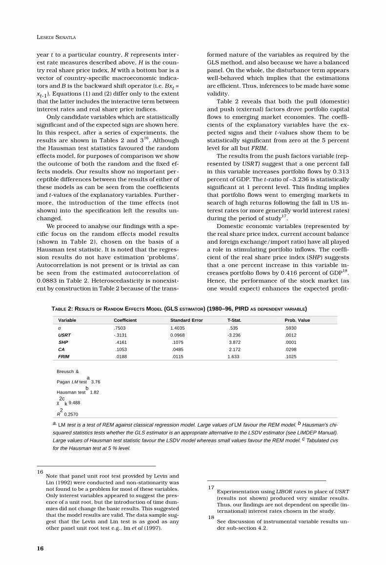
Only candidate variables which are statisticallysignificant and of the expected sign are shown here.In this respect, after a series of experiments, theresults are shown in Tables 2 and 316. Althoughthe Hausman test statistics favoured the randomeffects model, for purposes of comparison we showthe outcome of both the random and the fixed ef-fects models. Our results show no important per-ceptible differences between the results of either ofthese models as can be seen from the coefficientsand t-values of the explanatory variables. Further-more, the introduction of the time effects (notshown) into the specification left the results un-changed.

We proceed to analyse our findings with a spe-cific focus on the random effects model results(shown in Table 2), chosen on the basis of aHausman test statistic. It is noted that the regres-sion results do not have estimation ‘problems’.Autocorrelation is not present or is trivial as canbe seen from the estimated autocorrelation of0.0883 in Table 2. Heteroscedasticity is nonexist-ent by construction in Table 2 because of the trans-

formed nature of the variables as required by theGLS method, and also because we have a balancedpanel. On the whole, the disturbance term appearswell-behaved which implies that the estimationsare efficient. Thus, inferences to be made have somevalidity.

Table 2 reveals that both the pull (domestic)and push (external) factors drove portfolio capitalflows to emerging market economies. The coeffi-cients of the explanatory variables have the ex-pected signs and their t-values show them to bestatistically significant from zero at the 5 percentlevel for all but FRIM.

The results from the push factors variable (rep-resented by USRT) suggest that a one percent fallin this variable increases portfolio flows by 0.313percent of GDP. The t-ratio of –3.236 is statisticallysignificant at 1 percent level. This finding impliesthat portfolio flows went to emerging markets insearch of high returns following the fall in US in-terest rates (or more generally world interest rates)during the period of study17.

Domestic economic variables (represented bythe real share price index, current account balanceand foreign exchange/import ratio) have all playeda role in stimulating portfolio inflows. The coeffi-cient of the real share price index (SHP) suggeststhat a one percent increase in this variable in-creases portfolio flows by 0.416 percent of GDP18.Hence, the performance of the stock market (asone would expect) enhances the expected profit-

16Note that panel unit root test provided by Levin andLin (1992) were conducted and non-stationarity wasnot found to be a problem for most of these variables.Only interest variables appeared to suggest the pres-ence of a unit root, but the introduction of time dum-mies did not change the basic results. This suggestedthat the model results are valid. The data sample sug-gest that the Levin and Lin test is as good as anyother panel unit root test e.g., Im et al (1997).

17Experimentation using LIBOR rates in place of USRT(results not shown) produced very similar results.Thus, our findings are not dependent on specific (in-ternational) interest rates chosen in the study.

18See discussion of instrumental variable results un-der sub-section 4.2.

Variable Coefficient Standard Error T-Stat. Prob. Value

α .7503 1.4035 .535 .5930

USRT -.3131 0.0968 -3.236 .0012

SHP .4161 .1075 3.872 .0001

CA .1053 .0485 2.172 .0298

FRIM .0188 .0115 1.633 .1025

Breusch &

Pagan LM testa

3.76

Hausman testb

1.82

χ2c

k 9.488

R2

0.2570

TABLE 2: RESULTS OF RANDOM EFFECTS MODEL (GLS ESTIMATOR) (1980–96, PIRD AS DEPENDENT VARIABLE)

a. LM test is a test of REM against classical regression model. Large values of LM favour the REM model. b Hausman’s chi-

squared statistics tests whether the GLS estimator is an appropriate alternative to the LSDV estimator (see LIMDEP Manual).

Large values of Hausman test statistic favour the LSDV model whereas small values favour the REM model. c Tabulated cvs

for the Hausman test at 5 % level.


17

ability of investment in the countries under inves-tigation, enticing foreign portfolio inflows in theprocess19. The apparent statistical significance ofthe current account balance and the ratio of re-serves to imports variables can be interpreted asadditional country-specific indicators of creditwor-thiness20.

Further experimentation involving both real andnominal interest rates was conducted (results notshown). Real interest rates used were UKBONDSand RUSRT as explained above. In the main, theresults from using real interest rates were not thatdissimilar from those using nominal rates only.However, the strength of real interest in drivingportfolio flows was somewhat inferior to that ofnominal interest rate variables. For the sake of con-sistency with the previous literature, it was decidedto stick with the nominal interest rate variables. Itis, however, fair to infer that using either real (par-ticularly UKBONDS) or nominal interest rates tomeasure the push factors may not make muchmaterial difference to the findings.

Table 4, which is based on the differencingmethod, shows the relative importance of the pulland push factors in explaining portfolio inflows ineach country. While the results discussed aboveprovide a general picture of the significance of ourexplanatory variables they cannot be used, in theirpresent form, to assess the impact each of our ex-planatory variables had on the dependent variablein each country. To construct Table 4, we differen-tiate each of our variables (in each country) be-tween 1984 and 1994 period and multiply this re-sultant difference by the estimated coefficient foreach variable using the results from Table 2. This

procedure allows us to determine the extent towhich portfolio flows were being explained by thechange in our regressors in each country.

Table 4 reveals regional differences in the re-sults. In Latin American economies, the pull fac-tors as represented (in particular) by the real shareprice index dominate the push factors. On the other

hand, the push factors are more influential thanthe pull factors in Asian economies. These resultsmight be reflecting the fact that Latin Americaneconomies were able to obtain portfolio capital in-flows following serious economic policy reforms.21

The performance of the stock market may haveindicated bright investment prospects in the LatinAmerican economies. On the other hand, mostAsian economies have not experienced domesticeconomic problems to the extent that Latin Ameri-can economies have22. As a result, domestic eco-nomic factors in Asian countries may not have beenissues of concern to investors. Thus we would ex-pect that since there was nothing new in domesticfactors, then changes in external factors would in-stead be more likely to be the dominant factors inAsia.

We created USHPI, obtained as a product ofUSRT and SHP, to gauge the influence of the inter-active effects. A negative statistically significantcoefficient of this term would suggest the impor-tant facilitating role of the pull factors to the pushfactors. On the other hand, an insignificant coeffi-cient of this term would imply that portfolio flowswould occur on the basis of developments in USinterest rates irrespective of the domestic economicconditions.

Table 5 provides estimation results with USHPIincluded. The multiplicative variable is highly sig-nificant, with the expected negative coefficient, butsome (domestic) macroeconomic variables (i.e., CAand FRIM) have much diminished importance. Theexternal factor variable (USRT) also loses its sig-nificance and has an unexpected positive sign.Nevertheless, the significance of the multiplicativevariable indicates strong support for the hypoth-

Variable Coefficient Standard Error T-stat Prob. value

USRT -.3013 0.0990 -3.043 .0028

SHP .4268 .1086 3.930 .0001

CA .1116 .0496 2.252 .0258

FRIM .0224 .0132 1.695 .0922

F[12, 140) = 6.19 R2 = .3467 R

2 = .2908

Estimated Autocorrelation = .088296

Akaike info. Criteria = 4.852

N = 153 Degrees of Freedom = 140

TABLE 3: RESULTS OF FIXED EFFECTS MODEL (1980–96, PIRD AS DEPENDENT VARIABLE)

19We experimented with real share price index adjustedfor stock market liberalisation. To do this we createddummy variables to capture dates in which stock mar-kets were liberalised. We then regressed real shareprice index on these dummies and consequently re-placed real share price index by the resultantresiduals. Our results were similar to those that wereobtained here.

20We experimented with dropping Malaysia from the re-gression (results not shown) since it was suggested inSection 3 that, unlike most other countries, it hadexperienced negative portfolio inflows during most ofthe study period. Our basic results were not affected.

21Edwards (1999) makes a similar point.

22East Asia’s financial crisis started (in earnest) in 1997,i.e. outside our period of study.

LESEDI SENATLA

18

esis of an interaction between domestic and exter-nal economic factors.

Instrumental Variable EstimationAlthough the interest rate variables can reason-ably be taken as exogenous there is possibleendogeneity between portfolio flows and the shareprice index, the current account and foreign ex-change reserves. It could be argued that the cur-rent account balance, foreign exchange reservesand the share price index variables increased as aresult of portfolio inflows. The problem ofendogeneity (or correlation between regressors andthe disturbance term), however, exists only in thefixed effects but not the random effects model. Thefixed effects model is calculated based on OLSmethod while the random effects model relies onGLS method.

We chose as instruments one-period lagged val-ues of CA, FRIM and SHP variables. Table 6 presentsthe instrumental variable estimation results. Thepicture that emerges is very much the same as inTable 3. Thus, consistency of the estimates doesnot seem to have been affected by the suspectedendogeneity of the regressors.

Comparative results implicationsComparative results implications with the previ-

ous literature are not easy because of differencesin countries covered, estimation techniques and soforth. Still, the central issue is the same, viz. thequestion of the relative importance of the push andpull factors in driving portfolio capital flows to Asianand Latin American economies.

Fernandez-Arias (1996) and Calvo et al. (1993)conclude that emerging market economies aremostly vulnerable to external economic develop-ments. They argue that a rise in US interest rateswould lead to an outflow of capital from emergingmarket economies. According to these authors,domestic economic factors play no role in capitalmovements. Our results do not entirely supportthese authors’ strong policy conclusions. We findthat both the push and pull factors have signifi-cant influences on portfolio capital flows. But, wealso find that the relative importance of the push

and pull factors differ by region. Indeed, as shownabove, our findings suggest that the domestic (pull)factors – through the real share price index, in par-ticular – dominate the external factors in LatinAmerican economies. Only in the Asian economies’case do our results appear to concur with theseauthors’ findings in stressing the dominating im-portance of the push over the pull factors. The rea-sons for the regional differences were explainedabove.

Push factor Pull factors

Country USRT SHP FRIM CA

Argentina 1.76 2.54 0.77 0.39

Brazil 1.76 2.31 0.55 0.03

Chile 1.76 1.85 0.95 -1.17

Mexico 1.76 2.65 -0.92 1.24

Philippines 1.76 1.36 0.34 0.16

Malaysia 1.76 0.48 0.35 0.02

Thailand 1.76 0.94 0.75 0.10

Indonesia 1.76 0.81 0.07 -0.17

Korea 1.76 0.82 0.30 -0.01

TABLE 4: DECOMPOSITION OF THE PUSH AND PULL FACTORS BASED ON DIFFERENCING (1984–1994, PERCENTAGE OF

GDP).


α -6.1385 2.4285 -2.528 .0115

USRT .4681 0.2465 1.899 .0575

USHPI -.1276 .0373 -3.421 .0006

SHP 1.6063 .3626 4.430 .0000

CA .0698 .0482 1.448 .1476

FRIM .0081 .0118 0.684 .0494

Breusch &

Pagan LM testa

2.62

Hausman testbc

1.70

R2

0.3199

TABLE 5: RESULTS OF RANDOM EFFECTS MODEL (GLS ESTIMATOR) INCLUDING USHPI (1980–96, PIRD AS DEPENDENT

VARIABLE)

Notes a and

b the same as in Table 2.

c Tabulated critical values are the same as in Table 3.


19

Taylor and Sarno’s findings are most consist-ent with ours in emphasising the importance of boththe push and pull factors. But the details are dif-ferent. While their results suggested that interestrates are a more important determinant of portfo-lio flows to Latin America than to Asia, our resultssuggest the opposite.

Chuhan et al. (1998) find that global variablesare as important as domestic variables for LatinAmerica, and this is at odds with our findings. Againin the case of Asia their findings are the exact op-posite of ours. They find country-specific variablesto be more important than global variables in Asia.The limitations of Chuhan et al. and Taylor andSarno’s studies were highlighted (in Section 2)which may account for the differences between thefindings contained in this paper.

5. CONCLUSION

The messages of this paper are as follows. One isthat domestic policy makers in developing coun-tries are able to influence portfolio capital inflowsto their countries. Improvements in the domesticinvestment climate (resulting from economic re-forms) seem to be rewarded with portfolio inflows.Indeed, there is scope for even more portfolio in-vestments to occur in the future if the domesticinvestment climate continues to be favourable,since these economies invariably tend to be un-derweight in the portfolios of industrial countryinvestors (Claessens and Gooptu, 1994). It is worthnoting that all developing countries that aspire toaccess international capital markets or flows canlearn from the experience of the Asian and LatinAmerican economies. The key to receiving portfoliocapital flows is economic policy reform and stabil-ity, which provides favourable investment condi-tions, which together with the push factors (lowreturns elsewhere) tend to spur the inward move-ments of portfolio capital flows.

The second message is that interactive effectsare important. Nominal interest rates may havenegligible effects on portfolio flows when confidencein developing countries is low, and quite signifi-cant effects when confidence is high. This findingis consistent with the effective collapse in the mar-

ket for developing-country financial instruments athigh levels of risk. In effect, it does not seem realis-tic to suggest that the job of driving portfolio flowsshould be left either to external factors or domes-tic factors alone. Put differently, the push and pullfactors are individually necessary but neither isnecessarily a sufficient condition to ensure portfo-lio capital inflows.

REFERENCES

Adler, M., and B. Dumas (1975), ‘Optimal InternationalAcquisitions’. The Journal of Finance, vol. 30, no. 1,pp. 1–19.

Ahmed, M. and S. Gooptu (1993), ‘Portfolio InvestmentFlows to Developing Countries’. Finance and Devel-opment, pp. 9–12.

Baer, W and K. Hargis (1997), ‘Forms of External Capitaland Economic Development in Latin America: 1820–1997’, World Development, vol. 25, no. 11 pp. 1805–1820.

Bekaert, G. (1995), ‘Market Integration and InvestmentBarriers in Emerging Equity Markets’, The World BankEconomic Review, vol. 9, no.1 pp. 75–107.

Boyd, J. H., and B. D. Smith (1997), ‘Capital Market Im-perfections, International Credit Markets and Non-Convergence’. Journal of Economic Theory, 73 pp 335–364.

Brewer T. L., and P. Rivoli (1990), ‘Politics and PerceivedCountry Creditworthiness in International Banking’.Journal of Money, Credit and Banking, vol. 22, no.3,pp. 357–369.

Calvo A. G., L. Leiderman, and C. M. Reinhart (1993),‘Capital Inflows and Real Exchange Rate Apprecia-tion in Latin America: The Role of External factors’,IMF Staff Papers, 40 pp 108–151.

Cardoso, E. and I. Goldfajn (1997), ‘Capital Flows To Bra-zil: The Endogeinity Of Capital Controls’, IMF Work-ing Paper WP/97/115.

Chuhan, P., S. Claessens and N. Mamingi (1998), ‘Equityand Bond Flows to Latin America and Asia: The Roleof Global and Country Factors’. Journal of Develop-ment Economics, vol. 55, no. 2 pp. 439–463.

Claessens S. and S. Gooptu (1994), ‘Can Developing Coun-tries Keep Foreign Capital Flowing In?’ Finance andDevelopment, pp. 62–65.

Corbo, V., and L. Hernandez (1996), ‘MacroeconomicAdjustment to Capital Flows Inflows: Lessons FromRecent Latin American and East Asia Experience’. TheWorld Bank Research Observer vol. 11 no. 1, pp 61–85.

Edwards, S. (1999), ‘Capital Flows to Latin America’, in


USRT -.3498 .0971 -3.603 .0004

SHP .3393 .0987 3.437 .0008

CA .1007 .0502 2.009 .0464

FRIM .0278 .0131 2.115 .0361

F[12, 140) = 6.02 R2 = .3402 R

2= .2837

Estimated Autocorrelation = .096746

Akaike info. Criteria = 4.862

N = 153 Degrees of Freedom = 140

TABLE 6: RESULTS OF INSTRUMENTAL VARIABLE ESTIMATION

LESEDI SENATLA

20

International Capital Flows, edited by MartinFeldstein, National Bureau of Economic ResearchConference Report, The University of Chicago Press,London.

El-Erian, M. A. (1992), ‘Restoration of Access to Volun-tary Capital Market Financing: The Recent LatinAmerican Experience’. IMF Staff Papers vol. 39, no.1,pp. 175–194.

Eun, C. S. and S. Janakiramanan (1986), ‘A Model ofInternational Asset Pricing with A Constraint on theForeign Equity Ownership’. The Journal of Finance,vol. XLI, no.4, pp. 897–914.

Fernandez-Arias, E. (1996), ‘The new wave of private capi-tal inflows: Push or pull?’. Journal of DevelopmentEconomics, vol. 48, pp. 389–418.

Gertler, M. and K. Rogoff (1990), ‘North South Lendingand Endogenous Domestic Capital Market Inefficien-cies’. Journal of Monetary Economics 26, pp 245–266.

Gooptu, S. (1993), ‘Portfolio Investment Flows To Emerg-ing Markets’ in Portfolio Investment In DevelopingCountries, Edited by S. Claessens and S. Gooptu,World Bank Discussion Papers No. 228, The WorldBank, Washington DC, pp. 45–77.

Haque, N. H., M. S. Kumar, N. Mark and D. J. Mathieson(1996), ‘The Economic Content of Indicators of De-veloping Country Creditworthiness’. IMF Staff Papers,vol. 43 no 4 pp. 688–724).

Haque, N. H., N. Mark and D. J. Mathieson (1998), ‘TheRelative Importance of Political and Economic Vari-ables in Creditworthiness Ratings’ IMF Working Pa-per (1998) WP/98/46 http://www.imf.org/external/pub

Ishii, S. and S. Dunaway (1995), ‘Portfolio Capital Flowsto the Developing Country Members of APEC’, in Capi-tal Flows in the APEC Region, edited by M. S. Khanand C. M. Reinhart, IMF occasional paper no. 122,Washignton DC.

Jorion, P. and E. Schwartz (1986), ‘Integration vs. Seg-mentation in the Canadian Stock Market’. The Jour-nal of Finance, vol. 41, no. 3 (July 1986), pp. 603–616.

Kim, Y. (2000), ‘Causes of capital flows in developing coun-tries’. Journal of International Money and Finance, vol.16 pp. 235–253.

Kreicher, L. L. (1981), ‘International Portfolio Capital Flowsand Real Rates of Interest’. The Review of Economicsand Statistics, vol. 63, pp. 20–28.

Leland, H. E. and D. H. Pyle (1977), ‘InformationalAsymmetries, Financial Structure and Financial In-termediation’. The Journal of Finance, vol. XXXII, no.2,pp. 371–387.

Lensink R., and P.A. Van Bergeijk (1991), ‘The Determi-nants of Developing Country Access to the Interna-tional Capital Market’. Journal of Development Stud-ies, vol. 28 no.1, pp 86–103.

Levin, A and C. Lin (1992), ‘Unit Root Tests In Panel Data:Asymptotic and Finite-Sample Properties’, UniversityOf California, San Diego California.

Miller, N. C. and M. V. N. Whitman (1970), ‘A Mean-Vari-ance Analysis of United States Long-Term PortfolioForeign Investments’. Quarterly Journal of Econom-ics, vol. 84, no. 2, pp. 175–196.

Schadler, S., M. Carkovic, A. Bennett, and R. Khan (1993),‘Recent Experiences with Surges in Capital Inflows’,IMF Occassional Paper no. 108, Washington DC, De-cember.

Singh, A. (1995), ‘The Causes of Fast Economic Growthin East Asia’. UNCTAD Review, UN, New York andGeneva.

Taylor, M. P., and L. Sarno (1997), ‘Capital Flows to De-

veloping Countries: Long and Short Term Determi-nants’. The World Bank Economic Review, vol. 11. no.3, pp. 451–470.

Townsend, R. M. (1979), ‘Optimal Contracts and Com-petitive Markets with Costly State Verification’. Jour-nal of Economic Theory, vol. 21, pp. 265–293.

Turner, P. (1995), ‘Capital flows in Latin America: A NewPhase’, BIS Economic Papers 30. Basle: Bank for In-ternational Settlements, Monetary and EconomicDepartment.

UN (1994; 1995; 1996), World Economic and Social Sur-vey: Current Trends and Policies in the World Economy,United Nations, New York..

UNCTAD (1993 & 1997), World Investment Report:Transnational Corporations and Integrated Interna-tional Production, Geneva and New York, United Na-tions.

World Bank, World Debt Tables 1994–1995, ‘External Fi-nance for Developing Countries’, vol.1, WashingtonD.C, (1994).

MONEY LAUNDERING AND ELECTRONIC BANKING – CHALLENGES FOR SUPERVISORY AUTHORITIES IN THE SADC REGION

21

Money Laundering andElectronic Banking –Challenges for SupervisoryAuthorities in The SouthernAfrican DevelopmentCommunity (SADC) Region

Goememang Baatlholeng & EstherMokgatlhe1

INTRODUCTION

Globalisation and the liberalisation of financialmarkets have increased the risks of money laun-dering and, therefore, all countries that are inte-grated into the international financial systemshould put measures in place to combat all crimesthat generate ‘dirty’ money. The growth in electronicbanking also presents challenges to the war againstmoney laundering. Joyce (2001) has observed, that‘the progression of electronic commerce activity,electronic banking operations and electronic pay-ments technologies comprises a unique basket ofmoney laundering opportunities and threats to theindividual consumer, corporate business, commu-nity and governmental institutions’. Different agen-cies around the world gather statistics on moneylaundering but it is not easy to obtain accurate fig-ures because it is impossible to record all crimesthat generate ‘dirty’ money. Steven Philippsohn(2001) has noted that the features of the Internetthat make it ideal for commerce also make it idealfor money laundering. These features include,among others, speed, access, anonymity and thecapacity to extend beyond national borders. Theevents of September 11, 2001 have added anotherdimension to the meaning of money laundering. Itis no longer viewed as just ‘dirty’ money from crimi-nal activity, such as drug trafficking, extortion,arms smuggling and other crimes, but has beenbroadened to include ‘clean money’ that is used forthe ‘financing of terrorist activities’.

The objectives of this paper are to find out theextent of money laundering activities and the levelof development of electronic banking in the South-ern African Development Community (SADC) re-gion; to outline the supervisory challenges posedby these development; and to assess whether theregion is prepared for the challenges, such as, tocombat money laundering that could be facilitated

through electronic banking activities. The secondpart of the paper discusses the general backgroundon money laundering and electronic banking andthe relationship between the two. It touches on in-ternational initiatives and standards for combat-ing money laundering, and the Basel Committee’sposition on the development of electronic bankingand e-money activities. The third part, which formsthe core of the paper, focuses on the supervisorychallenges posed by money laundering and elec-tronic banking. It begins with a brief review of therationale for regulation and supervision of the fi-nancial sector and concludes by assessing whetherSADC countries will cope with the challenges pre-sented by a combination of money laundering andelectronic banking. Part four takes Botswana as acase study. It examines the development of elec-tronic banking in Botswana and the types of crimi-nal activities that could generate ‘dirty’ money. Thelaws that criminalise money laundering are identi-fied, and the various initiatives taken by the Fi-nancial Action Task Force (FATF), the Common-wealth and other international organisations to-wards combating money laundering, whichBotswana has adopted, are highlighted. The role ofthe central bank in electronic banking and anti-money laundering (Know Your Customer) supervi-sion will also be explored. The final part of the pa-per contains the conclusion and recommendationsfor supervisory authorities in developing countries.

GENERAL BACKGROUND ON MONEY

LAUNDERING AND ELECTRONIC BANKING

What is Money Laundering?Money laundering is described as a process bywhich the proceeds of crime (‘dirty’ money) are putthrough a series of transactions, which disguisetheir illicit origins and make them appear to havecome from a legitimate source (‘clean’ money)(Grabosky and Smith, 1998). By so doing crimi-nals avoid prosecution, conviction and confisca-tion of their ill-gotten funds. Sophisticated laun-derers involve many unwitting accomplices, suchas banks and securities houses, financial interme-diaries, accountants and solicitors, surveyors andestate agents, company formation agents and man-agement services companies, casinos, bullion andantique dealers, car dealers and others dealing inhigh value commodities and luxury goods. Thepoorly regulated institutions and services, and off-shore centres that offer guarantees of secrecy andanonymity are the most vulnerable (CommonwealthSecretariat, 2000).

Money laundering takes place in three stages,namely, placement, layering and integration, whichmay occur as separate and distinct phases; theymay also occur concurrently, or may overlap. Place-ment involves the actual disposal of cash proceedsderived from illegal activities. This might be done

1Both authors are Senior Bank Examiners in the Bank-ing Supervision Department, Bank of Botswana. Thepaper was originally prepared for the Supervisory Es-say Award, 2002 organised by the Financial Stabil-ity Institute of the Bank for International Settlementsin 2002, where it received a commendation.

GOEMEMANG BAATLHOLENG & ESTHER MOKGATLHE

22

by breaking up large amounts of cash into less con-spicuous smaller sums that are then deposited intoa bank, or by purchasing a series of monetary in-struments (money orders, travellers cheques) thatare then collected and deposited into accounts atanother location. Layering occurs when the illicitproceeds are separated from their source by en-gaging in a series of conversions or movements offunds to distance them from their source. Exam-ples of layering include telegraphic money trans-fers, purchase and sale of investments, resale ofacquired assets, and deposit of cash in banks. In-tegration gives apparent legitimacy to criminallyderived wealth by reintroducing the laundered pro-ceeds back into the economy to support legitimatebusiness activities and/or consumption.

Why Take Action Against Money Laundering?Money laundering is a criminal activity which canbring social evils if left unchecked. For example, itleads to disregard for the law and its ill-gotten gainscould be used to finance further crimes. Therefore,it is very crucial that this criminal activity is stoppedbefore it grows to uncontrollable levels.

Money launderers make large sums of moneyfrom various criminal activities such as drug traf-ficking, fraud, slavery, prostitution and corruption,which they could use to invest in any business ven-ture, and could ultimately gain control of the busi-ness ventures or companies. Once they are in thisposition, they could bribe and corrupt other busi-nessmen and government officials in the quest togain power. With their accumulation of economicand financial power, they could undermine nationaleconomies and disrupt democratic systems.

Another disturbing consequence of money laun-dering is that the accumulated money is transmit-ted around the globe frequently and quickly to anextent that it may end up causing distortions inexchange rates, money demand, international capi-tal flow and investment. In the process, intermedi-ary banks, can be exposed to prudential risks. Theabove effects of money laundering can distort gov-ernment macroeconomic policies as well as re-sponses to it (Commonwealth Secretariat, 2000).

International Initiatives and StandardsA number of international organisations have comeup with initiatives and standards to counter moneylaundering; this include the Financial Action TaskForce (FATF), International Monetary Fund (IMF),Commonwealth Secretariat, United Nations (UN)and the Basel Committee on Banking Regulationand Supervisory Practices. The FATF has published40 recommendations to serve as a comprehensiveregime against money laundering. These cover therole of national legal systems, the role of the finan-cial system and the strengthening of internationalcooperation. The IMF is of the view that the eco-nomic and financial reform policies it promotes arein line with the efforts aimed at defeating money

laundering activities (Commonwealth Secretariat,2000).

The 1988 Vienna Convention commits countriesthat sign up to criminalise drug trafficking andassociated money laundering, enact legal statutesfor the confiscation of proceeds of drug traffickingand empower their courts to order that banks’ fi-nancial or commercial records be made availableto law enforcement agencies, regardless of banksecrecy laws (Commonwealth Secretariat, 2000).

The Commonwealth Secretariat has drawn upa model law for the prohibition of money launder-ing which is targeted at common law countries, andit embraces all the issues covered by the 40 FATFrecommendations. In addition, this model law in-cludes an ‘all crimes’ money laundering offence.The Basel Committee has issued a statement ofprinciples, which require all banking institutionsto comply with all anti-money laundering meas-ures. (BIS, 2002).

Following the events of September 11, 2001, theFATF expanded its mission by issuing new inter-national standards to combat money launderingfor terrorist financing. In addition, the UN has calledupon all countries to ratify the 1999 UN Interna-tional Convention for the Suppression of the Fi-nancing of Terrorism and the UN Security CouncilResolution 1373 (2001).

Money laundering calls for an international re-sponse appropriate to the financial and economicrealities of each country. With increasing develop-ments in technology, the world is now confrontedwith electronic money laundering. Strengtheningthe prudential supervision and reputation of thefinancial system through effective anti-money laun-dering guidelines could substantially assist in theprevention of money laundering. The work of theFinancial Stability Forum (FSF) in raising interna-tional standards within offshore centres, both inthe area of financial regulation and anti-moneylaundering measures, is most welcome given thatit is in these centres criminals tend to find safehavens.

Electronic BankingTechnological developments have brought new op-portunities for banks. The advent of electronicbanking promises to expand the banks’ marketsfor new products and services. On the negative side,although banks have always been exposed to riskssuch as fraud and error, the magnitude of thoserisks and the swiftness with which they can cropup have changed dramatically due to the banks’dependence on the technological innovation in com-puters and telecommunication systems.

The BIS (1998) defines electronic banking as‘the provision of retail and small value bankingproducts and services through electronic channelsas well as large value electronic payments and otherwholesale banking services delivered electronically’.Such products and services can include deposit

MONEY LAUNDERING AND ELECTRONIC BANKING – CHALLENGES FOR SUPERVISORY AUTHORITIES IN THE SADC REGION

23

taking, lending, account management, the provi-sion of financial advice, electronic bill payment andthe provision of other electronic payments prod-ucts and services such as electronic money.

Electronic Banking Products and ServicesElectronic banking products and services are manyand are still evolving. They include, among others,card transactions, internet banking, electronicfunds transfer systems, home/telephone bankingservices, and electronic money. O’Hanlon andRocha (1993) have discussed these products andservices in detail while Grabosky and Smith (1998)have discussed them in the context of crime in thedigital age. A brief description of some of these prod-ucts and services is given below.

(a) Card Transactions

These enable users to carry out transactions froma location distant from the central database suchas a bank. The cards are inserted into a card readerwhere the total amount of purchases will be keyedin. The card reader will then produce a receipt re-questing the customer’s signature if the transac-tion has been approved or declined, which couldbe due to various reasons, like clearing house notresponding or lack of funds in the customer’s ac-count. Card transactions are done using creditcards and debit cards. Two types of card terminalsare available for use, namely, Automated TellerMachines (ATMs) and Electronic Funds Transferat Point of Sale (EFTPOS) (Grabosky and Smith,1998).

(b) Internet Banking

Internet banking refers to banking products andservices offered by institutions on the internetthrough access devices, including personal com-puters and other intelligent devices (Bank of Mau-ritius Guidelines on Internet Banking, 2001). MostInternet banks set up transactional websites andstill continue to operate their traditional ‘brick andmortar’ branches. Singh (1999) has noted that elec-tronic commerce remains a US and western basedactivity, thus it may take some time before the de-veloping world fully adopts Internet banking.

(c) Electronic Funds Transfer (EFT) Systems

In the inter-bank market electronic banking isnoted by the use of EFT systems such as the Soci-ety for Worldwide Interbank Financial Telecommu-nications (SWIFT), Fedwire, Interbank Data Ex-change (IDX), Clearing House for Interbank Pay-ment Systems (CHIPS) and Clearing House Auto-mated Payment Systems (CHAPS). The corporateEFT generally relates to the electronic transfer offinancial data and funds between companies andbanks in the settlement of business transactions.

(d) Home/Telephone Banking

This is carried out by using either a telephone or acomputer terminal located in a customer’s homeor office. This arrangement allows the customer todo almost all his banking transactions, such astransferring funds between accounts, stoppingcheque payments, ordering a cheque book or a bankstatement and many others. These services havepossibilities of being intercepted, which could be aserious security risk to customer accounts. The costimplications may also be too high in other areas,particularly developing countries.

(e) Electronic Money (E-money)

Electronic funds can now be stored on computersas well as on plastic cards, thereby enabling thefunds to be transferred through telecommunica-tions channels such as the internet. The BIS (1996)has defined electronic money products as ‘storedvalue’ or ‘prepaid’ products in which a record ofthe funds or ‘value’ available to a consumer is storedon an electronic device in the consumer’s posses-sion.

An arrangement is made between the bank andits customers whereby the customers request thebank to transfer funds from their bank accountsinto an electronic cash system. This system thengenerates and validates what are known as e-coins.The customer can then use the coins on the Internetusing software provided by electronic cash serviceproviders (Grabosky and Smith, 1998).

Since electronic money is becoming a popularmeans of payment, this raises policy concerns forcentral banks, which are the overseers of paymentsystems, managers of monetary policy, regulatorsof the financial system, and issuers of currency.Electronic money developments also bring in someconsumer protection issues, and gives rise to com-petition between traditional banks and non-bankissuers of electronic cash.

The accessibility of bank information throughcomputer terminals and telephones improves cus-tomer services and internal operations but, at thesame time, it increases the risks of error and abuseof the bank’s information. There is a possibility ofinformation getting lost and/or intercepted andultimately falling in the hands of criminals. It is,therefore, the responsibility of banks to ensure thatsecurity is adequate to guard against unauthor-ised access to customer information.

Operational risks can arise from customer mis-use, and from inadequately designed or imple-mented electronic banking and electronic moneysystems (BIS, 1998). Other disadvantages originatefrom organisational and legal implications of elec-tronic banking for banks.

Electronic banking continues to be adopted bybanks, retailers and customers because of the ad-vantages it has over traditional banking. Some is-sues such as legal obstacles and security loopholeswill take time to overcome.

LESEDI SENATLA

24

The Link Between Money Laundering andElectronic BankingThe Commonwealth (2000) has noted that thereare currently few case studies of money launder-ing through on-line banking. This could be becauseon-line banking is still at a developmental stage.On the other hand, Grabosky and Smith (1998)have observed that the use of telecommunicationstechnology in the banking sector has increased thechances of laundering dirty money. Given the in-creasing number of financial institutions provid-ing electronic banking products and services, andelectronic money activities, criminals are alsosharpening their skills to take advantage of thetechnology to further their activities.

Electronic money laundering also takes placethrough the process of placement, layering andintegration of the ill-gotten proceeds into the finan-cial system. Placement may occur through directelectronic transfer of funds to offshore institutionsor to ‘cyberspace’ or underground banks, withoutthe knowledge of the law enforcement agencies(Grabosky and Smith, 1998). Alternatively, elec-tronic money could be used to place dirty moneyinto the financial system without raising suspicionby carrying huge sums of hard cash or having toendure ‘Know Your Customer’ (KYC) procedures asis the case in face-to-face transactions.

The speed at which electronic transactions canbe processed facilitates the layering stage of elec-tronic money laundering. For example, a launderersitting in front of his personal computer can trans-fer electronic money into different accounts, at dif-ferent places within a day without raising suspi-cion. In the process dirty money is separated fromits illegal source. Electronic mail and encryptiontechnology enable the money launderers to pro-ceed with the layering of their illegal proceeds. Inthe case of internet banking, Philippsohn (2001)argues that there is legal debate as to where thetransaction actually occurred, hence prosecutorsfrom one jurisdiction face serious problems whenthey want to trace the audit trail of such transac-tions. Grabosky and Smith (1998) have noted that‘integration will be assisted by the development ofstored value cards, to which funds can bedownloaded from institutional sources.’

Electronic money laundering threatens tradi-tional due diligence systems. Therefore, electronicdue diligence, particularly the establishment of acomprehensive security control process, authenti-cation of electronic banking customers, establish-ment of clear audit trails for electronic bankingtransactions and privacy of customer information,should be initiated wherever there are electronicbanking activities. These risk management princi-ples have the potential to augment other anti-moneylaundering initiatives intended to combat electronicmoney laundering.

MONEY LAUNDERING AND ELECTRONIC

BANKING ACTIVITIES AND THE SUPERVISORY

CHALLENGES FACING THE SADC REGION

Rationale for Regulation of the FinancialSectorBamber et al (2001) have highlighted that the threemain objectives of financial regulation and super-vision of financial institutions are to sustain sys-temic stability, maintain the safety and soundnessof financial institutions, and protect consumers.Two types of regulation could be used to addressthe above objectives, namely, prudential regulationand conduct of business regulation. Prudentialregulation focuses on the solvency, safety andsoundness of financial institutions, whereas theconduct of business regulation focuses on how fi-nancial firms conduct business with their custom-ers, with emphasis on information disclosure, hon-esty and integrity of the firms. Both types of regu-lation cover consumer protection issues.

The KYC policies and procedures are the maintools used by financial institutions to combat moneylaundering. Sound KYC policies and procedures canensure the safety and soundness of financial insti-tutions. Failure to have KYC policies and proce-dures could lead to reputational, operational, legaland concentration risks for banks (BIS, 2001). Ona related point, the reliance of electronic bankingon information technology has created complexoperational and security loopholes, which could beexploited by criminals to perpetrate crime. Penetra-tion of banks’ computer systems by criminals couldcompromise the KYC policies and procedures thatthe banks would have established, and ultimatelythe safety and soundness of the financial institu-tion. Nieto (2001) has noted that the main chal-lenges faced by the financial regulator in the infor-mation technology era are, security and data pri-vacy, the global character of the provision of e-fi-nance services and the entrance of non-regulatednew intermediaries.

In light of the above, regulation and supervi-sion are essential for both anti-money launderingmeasures and electronic banking activities. How-ever, electronic banking is still developing and regu-lation should be done cautiously to avoid stiflinginnovation and creativity. Regulation is costly tothe regulated firms and sometimes it can be sostringent that it becomes a barrier to innovationand entry by new firms. It is important that theregulatory regime provides an environment thatwould promote the development of electronic bank-ing and also deter illegal activities.

Tables 1 and 2 below illustrate the potential formoney laundering activities and electronic moneydevelopments in some SADC countries.

It is noted from the table that four countriesout of eight are considered to have low potentialfor money laundering, and that all countries ex-


25

cept Tanzania, have some legislation against moneylaundering. South Africa and Mauritius, both ofwhich have vibrant financial sectors, are consid-ered to have high potential for money launderingand, unlike Zambia, which is also rated as havinghigh potential for money laundering in the bank-ing sector, they have legislation in place, that is,the Financial Intelligence Act, 2001 (South Africa)and the Anti-money Laundering and CorruptionAct, 2000 (Mauritius). Namibia, Lesotho andSwaziland also have legislation/guidelines on anti-money laundering measures.

A worrying situation is the fact that reports ofcorruption in high places have significantly in-creased in some of the countries rated low, suchas Zimbabwe and Malawi. The Global CorruptionReport (2001) has reported that there is not muchpolitical will from Southern African leaders to com-bat corruption. It further noted that the anti-cor-

ruption institutions that have been set up are notindependent from government, and as a result theyfail to probe senior officials suspected of corrup-tion.

Information on electronic banking and elec-tronic money activities is not readily available fordeveloping countries. This is probably because thedevelopment of these activities is still at an earlystage for these countries. Out of the four countriesfor which information was available, we noted thatSouth Africa and Mauritius were a step ahead ofothers in electronic banking and electronic moneyactivities, possibly because they already have vi-brant financial services sectors. These two coun-tries have made significant progress in creating thenecessary legislative arrangements and proceduresfor the monitoring and management of electronicbanking activities by both the regulators and thefinancial institutions.

Zimbabwe, which also has a well-developedbanking sector, has limited electronic banking ac-tivities. However, it does not have any specific leg-islation or guidelines governing these activities. The

TABLE 1-POTENTIAL FOR MONEY LAUNDERING ACTIVITIES IN SELECTED SADC COUNTRIES

Country Potential for money launderingActivities

Regulation Remarks

Low Medium High

Botswana _ Proceeds of SeriousCrime Act, 1990.

Banking Act, 1995.

Corruption and EconomicCrime Act, 1994

No indication that any significantamount of money laundering istaking place.

No statute specifically called theprevention of money launderingAct. The anti-money launderingprovisions are in several statutes.

Malawi _ Banking Act, 1989 Not considered a centre for moneylaundering.

Anti-Money laundering Act hasbeen drafted.

Mauritius _ Anti-money Launderingand Economic Crime Act,2000

Has a domestic drug consumptionproblem and a vibrant financialservices sector.

Seychelles _ Anti-money LaunderingAct, 1996

The Islands are neither asignificant producer nor a transitpoint for illicit narcotics.

South Africa _ Financial IntelligenceCentre Act, 2001

Major financial centre in subSaharan Africa

Major transhipment point forcocaine and heroine trafficking.

World largest consumer ofmandrax.

Corruption becoming a seriousproblem.

Tanzania _ Not available No regulation regarding the use ofthe banking system for purposesof money laundering.

Zambia _ Narcotic Drugs andPsychotropic substancesAct, 1993

Corruption Practices Act

It is reported that new bankingregulation to combat moneylaundering are being drafted.

Zimbabwe _ Serious Offences(confiscation of profits)Act

Prevention of CorruptionAct.

Reports of corruption in highplaces have significantlyincreased.

Source: Briscoe (1999)2

2Because of the developments that are taking place inthe area of money laundering, some of the informa-tion in the table may have changed by time of print.

LESEDI SENATLA

26

country relies on existing laws and regulations tomonitor these developments (Reserve Bank of Zim-babwe Annual Report, 2000). In Namibia, the Com-mercial Bank of Namibia, First National Bank andStandard Bank all offer some electronic bankingservices (Bank of Namibia, 2002).

What are the Supervisory Challenges?Criminals have discovered that crime can be car-ried out with fewer risks through the use of com-puters than when using traditional ways of bankrobberies and other crimes; this is a direct resultof technological development. It is imperative, there-fore, for regulators and bankers to review systemsand procedures used to combat money launderingand to monitoring electronic banking activities soas to manage new risks and challenges broughtabout by rapid technological changes. The chal-lenges presented by electronic banking and elec-tronic money laundering include, but are not lim-ited to, risk management challenges; strengthen-ing KYC requirements especially for electronic prod-ucts and services; setting up the necessary infra-structure to attract electronic banking and devel-oping national strategies to combat money laun-dering; capacity building for supervisory authori-ties and addressing problems brought about byinformal financial sector. A discussion of these chal-lenges follows below.

(a) Risk Management Challenges

Electronic banking offers a number of risk man-agement challenges for the supervisory authorities.

The Electronic Banking Group (EBG) of the BIS hasobserved that electronic banking does not intro-duce new risks to banking, instead, it makes thealready existing risks more precarious, in particu-lar, operational risk, reputational risk and strate-gic risk. The EBG has highlighted the following assome of the risk management challenges presentedby electronic banking activities (Risk ManagementPrinciples for Electronic Banking, 2001).

(i) The speed of change relating to technologicaland customer service innovation in electronicbanking is unprecedented. Historically, newbanking applications were implemented overrelatively long periods of time and only after in-depth testing. Today, however, banks are expe-riencing competitive pressure to roll out newbusiness applications in very compressed timeframes – often only a few months from conceptto production. This competition intensifies man-agement challenge to ensure that adequate stra-tegic assessment, risk analysis and securityreviews are conducted prior to implementingnew electronic banking applications.

(ii) Transactional electronic banking websites andassociated retail and wholesale businessapplications are typically integrated as muchas possible with legacy computer systems toallow more straight-through processing ofelectronic transactions. Such straight-throughautomated processing reduces opportunities forhuman error and fraud inherent in manualprocesses, but it also increases dependence onsound systems design and architecture as wellas system inter-operability and operationalscalability.

(iii) Electronic banking increases banks’dependence on information technology, thereby

3Electronic money developments are treatedas part of electronic banking.

Country Electronic Money Developments Regulation/Guidelines Remarks

Mauritius E-money has not been introduced bydomestic banks.

Several commercial banks offer card-based payment services, such as,credit and debit cards, and direct debit.

Some banks offer telephone banking,home banking and internet banking.

Electronic Transfer Act,2000.

Guidelines on internetbanking.

All licensed institutionsseeking to launch transactionalwebsites are required to obtainprior approval of the Bank ofMauritius.

South Africa Development of network-based productsis still in early stages.

E-money products are available and canbe activated through ATMs, telephonedevices, personal computers, intelligentcards and card reading devices.

Position paper on Electronicmoney issued by the SouthAfrican Reserve Bank inApril 1999.

There are about 600 000 on-linebanking customers.

Tanzania Efforts are being made by multi-nationalbanks to offer electronic banking and e-money schemes.

Guidelines on theintroduction and operation ofauditable card basedelectronic money schemes.

The guidelines provide that theBank of Tanzania as regulatorof the banking industry, willundertake some roles andresponsibilities in supportingoperations of any authorisedinter-bank auditable e-moneyschemes based on paymentcards.

Zambia No development in e-money Not available Zambia is participating in theCOMESA Mondex electroniccash application project.

TABLE 2 – ELECTRONIC BANKING AND ELECTRONIC MONEY DEVELOPMENTS IN SOME SELECTED SADC COUNTRIES

Source:CPSS Survey of Electronic Money Developments (2001)2


27

increasing the technical complexity of manyoperational and security issues and furtheringa trend towards more partnerships, alliancesand outsourcing arrangements with thirdparties, many of whom are unregulated. Thisdevelopment has been leading to the creationof new business models involving banks andnon-bank entities, such as Internet serviceproviders, telecommunication companies andother technology firms.

(iv) The Internet is ubiquitous and global by nature.It is an open network accessible from anywherein the world by unknown parties, with routingof messages through unknown locations andvia fast evolving wireless devices. Therefore, itsignificantly magnifies the importance ofsecurity controls, customer authenticationtechniques, data protection, audit trailprocedures, and customer privacy standards.

The above risk challenges could also exacer-bate money laundering activities. For example, therolling out of new business in a very short timeframe could lead to banks attracting business fromcriminals because the screening process would nothave been thorough. It is also possible thatoutsourcing arrangements with third parties, mostof whom may be unregulated, could result in bankshaving relationships with companies controlled bycriminals. The accessibility of the Internet world-wide also provides an opportunity for electronicmoney laundering, which threatens to be a men-ace in the digital age.

It is, therefore, important that SADC supervi-sors see to it that banks in their jurisdictions ad-here to the risk management principles for elec-tronic banking, which are grouped into three broadareas of board and management oversight, secu-rity controls, legal and reputational risk manage-ment.

(b) Strengthening KYC Requirements

According to the BIS consultative document onCustomer Due Diligence (2001), national supervi-sors are expected to set out supervisory practicesgoverning banks’ KYC programmes, monitor thatbanks apply sound KYC procedures and that theyare maintaining ethical and professional standardson a continuous basis. This challenge is bestachieved by incorporating the KYC requirementsin the laws that govern banks. The KYC require-ments should cover procedures for identifying on-line customers. On-site compliance examinationsshould be conducted to check whether banks com-ply with the provisions of the law. The examinationshould review customer files, sample accounts andlook for any suspicious transactions, and assessthose suspicious accounts that would have beenpicked by banks’ systems. The examination shouldalso focus on both the technical and non-technicalaspects of electronic banking activities. The overalllevel of risks that electronic banking activities pose

to the institution and the adequacy of the ap-proaches adopted to manage those risks should bethoroughly reviewed during the examination proc-ess.

The BIS recommends that the law should pro-vide firm supervisory actions for those institutionsthat fail to comply with the KYC requirements. TheCommonwealth Secretariat advocates a review ofbanking secrecy laws and enactment of the neces-sary amendments to ensure that financial institu-tions’ records can be made available to competentauthorities. The ultimate goal is meant to achievea safe and sound banking sector, and to protectthe integrity of the financial system.

(c) Adopting International Standards Against

Money Laundering and Adhering to the Risk

Management Principles for Electronic Banking

The region should work hard towards meeting in-ternational standards against money launderingand implementing the risk management principlesin order to promote the safety and soundness ofelectronic banking activities. SADC should encour-age member countries to adhere to internationalstandards against money laundering by harmonis-ing the legislative and institutional mechanisms sothat the region does not face regional reputationalrisk emanating from some non-cooperating mem-bers.

Money laundering and electronic banking ac-tivities can be carried out across borders. To avoidregulatory arbitrage and safeguard the integrity ofboth domestic and international banking systems,supervisors in the SADC region should work to-wards harmonising their banking laws, particularlyKYC standards. By so doing, they would discour-age criminals who may wish to start their activitiesin countries with weak legislation.

(d) Setting up the Necessary Infrastructure to

Attract Electronic Banking Activities and

Developing National Strategies Against Money

Laundering

O’Hanlom and Rocha (1993) predicted that ‘elec-tronic retail banking will replace traditional formsof banking in the next millennium, on a worldwidescale…because it offers greater convenience, speedand information than traditional banking services’.These are good reasons for supervisors, in collabo-ration with their governments, to provide an ena-bling environment for the development of electronicbanking activities.

The supervisory authorities in the SADC regionhave to develop guidelines for their specific juris-dictions for the provision of electronic banking andelectronic money services and products. Theyshould also establish national strategies againstmoney laundering, such as the formation of na-tional co-ordinating committees; criminalisingmoney laundering, setting financial sector obliga-tions and establishing a central reporting agency

LESEDI SENATLA

28

that would process/investigate reports, providefeedback to reporting institutions, and compile sta-tistics and trends on money laundering activities.

(e) Capacity Building within the Supervisory

Authorities

As much as supervisors expect banks to recognise,address and manage the risks brought about byelectronic banking activities, they should also bein a position to comment authoritatively on whetheror not banks respond prudently to all the electronicbanking risk management challenges. This can beachieved by ensuring that supervisors get the nec-essary training in electronic banking activities.Supervisors should be able to review the electronicbanking activities as and when the banks intro-duce them, and give advice, particularly to thoseinstitutions that may lack the experience and ex-pertise in this new business area. It is also essen-tial to enhance the general skills levels of supervi-sory staff to a level where they would keep pacewith financial innovation and development, moreespecially in risk management practices.

(f) The Informal Sector and other Illegal Entrants

in the Electronic Banking Sector

The informal financial sector is very active in manycountries (Commonwealth, 2000) and because itis unregulated in most SADC countries, the regioncould still become a safe haven for launderers oncecomprehensive anti-money laundering measuresare applied to the formal financial sector. It is, there-fore, important that an anti-money laundering leg-islation be extended to all sectors of the economyand that guidelines for electronic banking activi-ties should apply to both banking and non-bank-ing entities.

How Far is the Region in Addressing theAbove Challenges?The SADC region has a number of regional group-ings, which focus on integrating the political, andsocio-economic activities of member countries andon the harmonisation and facilitation of cross-bor-der financial services by the regulatory and super-visory authorities. Three such groupings are par-ticularly relevant when discussing electronic bank-ing and anti-money laundering activities. They arethe SADC Committee of Central Bank Governors,the East and Southern Africa Banking SupervisorsGroup (ESAF) and the Eastern and Southern Afri-can Anti-money Laundering Group (ESAAMLG).The Committee of Central Bank Governors’ activi-ties focus on broad central banking issues, e.g.,economic convergence. ESAF has the mandate tocoordinate all banking supervision related train-ing in the region. ESAAMLG is spreading the anti-money laundering message to all members of thegrouping, and assisting member countries tostrengthen the review of money laundering meth-ods and counter measures.

In a bid to address the problem of the informalsector, some member countries regulate activitiessuch as money lending and other ancillary finan-cial service providers (Central Bank of LesothoSupervision Department Annual Report, 2000).Others are working on policy guidelines for microfinance institutions. ESAF envisages a harmonisedapproach to micro finance in the region. The illegalelectronic banking and electronic money launder-ing activities are relatively new pursuits and itwould take sometime for the region to understandand combat such activities.

BOTSWANA AS A CASE STUDY

Botswana is a middle-income country in SouthernAfrica with a per capita GDP of US $3000 per an-num (SADC Review, 2001) and a small but thriv-ing financial sector. The country has differentclasses of banks, insurance companies, pensionfunds, collective investments undertakings, amoney and capital market, an international finan-cial services centre, specialised government ownedfinancial institutions and other small scale infor-mal financial service providers. The Ministry of Fi-nance and Development Planning (MFDP) and theBank of Botswana are the two regulatory and su-pervisory authorities of the above institutions. Thecentral bank is responsible for the supervision ofcommercial banks, investment/merchant banks,collective investment undertakings, Botswana Sav-ings Bank, IFSC activities (offshore banks), andbureaux de change. MFDP regulates insurance,pension funds and non-bank financial institutions.Botswana is a member of ESAF, ESAAMLG andSADC Committee of Central Bank Governors.

Electronic Banking Developments inBotswana

(a) Card Transactions

Botswana has not conducted any survey on theextent of electronic banking and e-money activi-ties as yet. However, the local financial institutionsare following the international trend by introduc-ing electronic banking services and products as andwhen they feel it is the right time to do so. Cardtransactions are the most common form of elec-tronic banking activities in Botswana. ATMs wereintroduced in the 1990s (Bank of Botswana An-nual Report, 2001). Barclays Bank, First NationalBank and Standard Chartered Bank issue VisaElectron badged cards, which can be used at anyATM that has a visa sign anywhere in the world.

(b) Corporate Electronic Products

Corporate electronic products available in theBotswana market include cash management serv-ices (First National Bank and Standard CharteredBank), corporate access terminal systems (StanbicBank), business master (Barclays Bank), sweeping


29

facility (Standard Chartered Bank and StanbicBank), and automated regular payments and col-lections services.

(c) Other Products and Services

First National Bank offers on-line banking serv-ices known as video bank, which is ‘a remote bank-ing service that offers business customers the con-venience of 24-hour secure desktop banking fromtheir own homes or offices, using the Internet as adelivery platform’ (First National Bank, May 2002).Barclays Bank offers telephone banking services(Barclays Tariff Guide, 2002). In the inter-bankmarket the SWIFT system is widely used for bothdomestic and international money transmission.

(d) Botswana National Payments System

The financial institutions, Botswana Governmentand the Bank of Botswana are working together todevelop a modern national payments system. Theautomation of the clearing house has been com-pleted. This means that cheque details are now readelectronically. Other initiatives that have been em-barked upon include the introduction of an elec-tronic funds transfer system for high volume lowvalue payments, the implementation of a large valuelow volume electronic transfer system, and the es-tablishment of an automated and comprehensivesettlement system. The committee responsible forthese developments is aiming at having a modern-ised payments system that will comply with inter-nationally accepted standards by 2005 (Bank ofBotswana Annual Report, 2001).

Anti-Money Laundering Measures inBotswanaAs shown in Table 1, Botswana was considered tohave low potential for money laundering three yearsago (Briscoe, 1999). However, criminal activitiesexist which could generate ‘dirty’ money such asdiamond smuggling, poaching, motor vehicle theft,and armed robberies. Moreover, the liberalisationof exchange controls in 1999, the setting up of theinternational financial services centre in 2000, andthe advent of electronic commerce could increasethe potential for money laundering. However, de-spite the electronic banking developments, thecountry is still largely a cash based society.

Botswana has in place, a national coordinatingcommittee on anti-money laundering measures,legislation that criminalises money laundering (TheProceeds of Serious Crime Act, 1990) and interna-tional cooperation with organisations such as theUN, IMF, and the Commonwealth Secretariat. Thecountry has incorporated the basic requirementsof the FATF and Basel Statements of principles intoits Banking Act, 1995. It has also ratified the es-sential international conventions against moneylaundering and related crimes, such as the 1988Vienna Convention and the 1999 UN Conventionfor the Suppression of the Financing of Terrorism.

Work needs to be done to broaden the defini-tion of the financial sector to ensure that all whoare likely to be involved in money laundering arecovered and to establish appropriate financial sec-tor obligations. A supportive effective enforcementstructure with centralised reporting point for sus-picions of money laundering and trained financialinvestigators is also essential.

The Role of Bank of BotswanaThe Bank of Botswana ensures that there is publicconfidence in, inter alia, the solvency of financialinstitutions through constant regulatory surveil-lance and effective prudential controls over thedomestic financial system. The Bank conductsregular on-site examinations to check for compli-ance with available anti-money laundering legisla-tion and to verify that the financial institutions haveproper systems in place to manage risks emanat-ing from electronic banking related activities. Inaddition guidelines are issued from time to time toassist banks to address new developments in bank-ing and finance.

SUMMARY AND CONCLUSIONS

In this paper, we have shown that money launder-ing activities are increasing all over the world. Wehave gone further to note that technological devel-opments have brought knew products and serv-ices in banking, some of which have opened a bas-ket of money laundering opportunities and threats.

Most SADC countries were shown to have highpotential for money laundering. On a positive note,most member countries had legislations againstmoney laundering which have to be refined to bein line with international standards. Regarding elec-tronic banking activities, it was noted that most ofthe countries in the region did not have guidelines/legislation for electronic banking activities, exceptSouth Africa and Mauritius.

On the basis of the above conclusions, it is ad-visable that SADC countries should establish na-tional coordinating committees to oversee anti-money laundering initiatives. These committeesshould review and strengthen all the anti-moneylaundering legislation to bring them to internationalstandards. The countries should further considerincorporating electronic due diligence in their anti-money laundering policies and procedures. Indi-vidual countries should conduct surveys to ascer-tain the extent of electronic banking and electronicmoney activities in their jurisdictions, and draftguidelines on how to manage risks in electronicbanking based on the BIS model.

Policy responses to the implications of e-moneyon monetary policies of individual countries shouldalso be considered. In addition, countries will haveto set aside resources for public education to sen-sitise consumers on the security risks they facewhen using electronic banking products and on the

LESEDI SENATLA

30

dangers of money laundering to democratic socie-ties. Finally, capacity building in the areas of in-formation technology in supervisory and law en-forcement authorities should be made a priority.Almost all countries will in future, require infor-mation technology bank examiners, and trainedfinancial investigators.

REFERENCES

Bamber, R., Falkena, H., Llewellyn, D. & Store, T (2001)Financial Regulation in South Africa. Revonia. SouthAfrican Financial Sector Forum.

Bank for International Settlements (July 1989). Risks inComputer and Telecommunications Systems.

Bank for International Settlements (March 1998). RiskManagement for Electronic Banking and ElectronicMoney Activities.

Bank for International Settlements. (May 2001). RiskManagement Principles for Electronic Banking.

Bank for International Settlements. Implications for Cen-tral Banks of the Development of Electronic Money –October 1996.

Banking Act, 1995. Botswana

Bank of Botswana Annual Report 2001

Barclays Bank of Botswana Limited Tariff Guide, 2002.

Briscoe, A. (1999). Banks and the Control of Money Laun-dering. London. Carlton Laws.

Carse, D. (1999). Keynote speech by the Deputy ChiefExecutive of the Hong Kong Monetary Authority, atthe ‘Symposium on Applied R&D:Enhancing GlobalCompetitiveness in the Next Millennium’, about theRegulatory Framework of E-Banking. BIS Review 108/1999.

Central Bank of Lesotho Supervision Report for 2000.

Commonwealth Secretariat (2000) A Model of Best Prac-tice for Combating Money Laundering in the FinancialSector. Prepared by Sue Thornhill and Michael Hylandof MHA Consulting. London.

Committee on Payments and Settlements Systems (CPSS)Survey of e-money developments (BIS, 2001).

Dale, P. (May 2002) Regional Report, Southern Africa.www.globalcorruptionreport.org.

Federal Reserve Commercial Bank Manual (November2001) Electronic banking.

Financial Action Task Force on Money Laundering An-nual Report 2000–2001.

Goodhart, C. Hartmann, P, Llewellyn, D, Rojas-Sua’rez,L &Weisbrod, S. (1998). Financial Regulation: Why,How and Where Now? London. Routledge.

Grabosky, P.N. & Smith, R. (1998). Crime in the DigitalAge: New Jersey. Transaction Publishers/FederationPress.

Hawkins, John. ‘Banking for International SettlementsPapers No.7’, Electronic Finance and Monetary Policy.

Eedes, J. (2001). Traditional vs. Virtual Banking. Finan-cial Mail Survey. Supplement to Financial Mail. Pp.8–10. Johannesburg.

Joyce, B.P. (2001). E-Diligence: Money Laundering Risksin the Electronic Arena. Journal of Money LaunderingControl, Volume 5, No. 2, 2001.

Mboweni, T. (1999) Address by Governor of the SouthAfrican Reserve Bank, at the Sun Microsystems Con-ference, on E-money and its impact on the CentralBank’s Operations. Midrand. BIS Review 109/1999.

Nieto J. Maria. ‘Banking for International Settlements

Papers No. 7’, Reflections on the Regulatory Approachto e-finance.

Official SADC Trade, Industry, and Investment Review –2001.

O’hanlon, John & Rocha, Marie. (December 1993) Elec-tronic Banking for Retail Customers. Banking Tech-nology Ltd. London

Philippsohn, S. (2001) ‘Dangers of New Technology – Laun-dering on the Internet’, Journal of Money LaunderingControl, Vol.5, No.1

Schilder, A.(2001) ‘Banking in the New Economy – Su-pervisory Perspective’, BIS Review 16/2001.

Singh, Didar A.(October 1999) Electronic Commerce: Is-sues for the South. Trade Related Agenda Develop-ment and Equity Working Papers. South Centre.(www.southcentre.org)

South African Reserve Bank – Bank Supervision Depart-ment Annual Report 2000.

Stanbic Bank Botswana Limited, Tariff Guide, 2002.

United Nations Security Council Resolution 1269 (1999)and Resolution 1373 (2001).

www.bis.org (May, 2002)

www.bon.com.na (May 2002)

www.bom.intnet.mu (May 2002)

www.esaf.org (May, 2002)

www.fnbbotswana.co.bw (May 2002)

www.oecd.org/fatf (May, 2002)

www.rbz.zm (may 2002)

www.resbank.co.za (May, 2002)

www.SADCbankers.org (May, 2002)

www.standardchartered.com (May, 2002)

GARCH MODELLING OF VOLATILITY ON OPTION PRICING: AN APPLICATION TO THE BOTSWANA MARKET

31

GARCH Modelling ofVolatility on OptionPricing: An Application tothe Botswana Market

Pako Thupayagale1

INTRODUCTION

This paper is motivated by an interest in how un-certainty and volatility affect the pricing of assets;in particular for financial assets where the currentprice is in part determined by expectations aboutthe future price, including the associated uncer-tainty. The analysis of such pricing raises issuesat both the theoretical and empirical level. Theorymay be able to help provide a framework to indi-cate how optimal pricing should be determined.However, the next step of empirical input and, morespecifically, obtaining relevant measures of volatil-ity in practice, raises further challenges.

In this paper, both these aspects are examinedin relation to a particular form of financial assetknown as an option, the purpose of which is tohelp investors hedge their exposure to volatility inasset prices. The approach taken here is, by ne-cessity, at a highly technical level, which may notbe immediately accessible to all readers. However,the various concepts and results that are presentedare accompanied by non-technical explanationsincluding, at the end of the paper, a glossary ofterms for easy reference (see appendix).

In conventional econometric models, the vari-ance of the disturbance is assumed to be constantboth unconditionally and conditionally. However,the phenomenon of changing variance andcovariance is often encountered in financial timeseries. The growing interest around models ofchanging variance and covariance has been moti-vated by their suitability both in describing the so-called ‘stylised facts’ of many economic and finan-cial variables, and in the pricing of contingent as-sets. An example of a contingent asset is an op-tion, which allows the option owner the right, butnot the obligation, to trade the underlying asset ata given price in the future.

In option pricing, the uncertainty associatedwith the future price of the underlying asset is themost important determinant in the pricing func-tion2. As volatility increases, the probability that

the financial asset will perform either exception-ally well or very poorly rises. For the owner of theasset these outcomes tend to offset each other;however, this is not the case for the owner of a callor put. In particular, the owner of a call option ben-efits from price increases but has limited downsiderisk in the event of price decreases, since the mostthat he can lose is the price of the option. Simi-larly, the owner of a put option benefits from pricedecreases but has limited downside risk in the eventof price increases. Therefore, the value of both callsand puts increases as volatility increases; hence,pricing an option involves valuing volatility.

In general, the models of changing variance andcovariance are called ‘volatility models’. The mainrepresentatives of this class of models are theAutoregressive Conditional Heteroscedasticity(ARCH) models (Engle, 1982) and the GeneralizedARCH (GARCH) models (Bollerslev, 1986). Thesemodels allow the conditional variance to changeover time as a function of past errors, leaving theunconditional variance constant. Option price es-timates derived from ARCH models can be used totest whether observed market options are efficientlypriced. This is because ARCH models capture thedynamic behaviour of market volatility using spe-cific volatility equations of the asset-return serieswithout presupposing any option-pricing formula,or using observed option prices. However, GARCHmodels are preferred since they are capable of re-flecting changes in the conditional volatility of theunderlying asset in a parsimonious manner.

In this paper the GARCH Option Pricing Model(OPM) is employed in order to examine the efficiencyof a hypothetical foreign currency option marketin Botswana3. The popular GARCH (1,1) specifica-tion is employed in the estimation of volatility forthe continuously compounded returns of the ex-change rate between the Pula and two currencies:the US dollar and the British pound. This forecast-ing method provides one common conditional vola-tility estimate for both call and put option pricesobtained by solving the option valuation problemvia Monte Carlo simulations. Such estimated prices,for different strike prices and maturities, are com-pared with the option prices prevailing in the localcurrency options market to evaluate its efficiencyin pricing options. The results obtained indicatethat the GARCH (1,1) OPM generally underpricescalls and overprices put options.

The paper is organised as follows. Section 2considers models of changing variance, with spe-cial attention given to observation-driven models,in particular the GARCH model. The pricing of con-tingent assets is discussed in Section 3. The lead-

1Dealer in the Financial Markets Department of theBank of Botswana. The paper was developed while theauthor was doing his MSc in economics at the Univer-sity of Warwick. The author is grateful for useful com-ments from colleagues at the Bank of Botswana andfrom his supervisor at Warwick University.

2See Bollerslev et al (1992).

3Some commercial banks in Botswana trade in cur-rency options. We use European currency options toproxy Botswana currency options (i.e., by convertingthose prices into their Pula equivalent).

PAKO THUPAYAGALE

32

ing role of the Black-Scholes Option Pricing For-mula (BSOPF) is highlighted. The next section re-views some theoretical and applied work into op-tion pricing theory when the Black-Scholes as-sumption of constant volatility is relaxed. Section5 presents the analysis of the continuously com-pounded returns of the US dollar/Pula and Britishpound/Pula exchange rates, and the estimation ofthe GARCH (1,1) process. Section 6 discusses theresults of the GARCH (1,1) OPM and evaluates itsstatistical properties vis-à-vis the prevailing cur-rency option prices, as a test for market efficiency.Section 7 concludes the analysis.

MODELS OF CHANGING VARIANCE

Volatility models can be categorised into observa-tion and parameter-driven models, where theformer express the variance (σt) in terms of pastobservations and the latter adopt a direct approachin which σt is modelled by an independentstochastic process. The most familiar example ofan observation-driven model is the ARCH modeldeveloped by Engle (1982), which can account forthe difference between the unconditional and theconditional variance of a stochastic process. TheARCH process allows the conditional variance tovary over time, leaving the unconditional (or longrun) variance constant.

In this model, the variance is modelled directlyas a linear function of the squares of past observa-tions:

σ α α αt t q t qy y20 1 1

2 2= + +− −K (1)

with α0 > 0 and αi ≥0, i=1,…,q, to ensure that theconditional variance is positive.

A more general representation of the abovemodel is the Generalised ARCH (GARCH) processintroduced by Bollerslev (1986). The GARCH mod-els are capable of capturing leptokurtosis, skewnessand volatility clustering4, which are the three fea-tures most often observed in high frequency finan-cial time series data.

In the GARCH model, the conditional varianceis specified as:

σ α α α β σ β σt t q t q t p t py y20 1 1

2 21 1

2 2= + + + + +− − − −K K

(2)

where the inequality restrictions α0>0, αi≥0, for i= 1, …,q, and βi ≥0 for i = 1,…,p, are imposed toensure that the conditional variance is strictlypositive. That is, the conditional volatility is speci-fied as in (1) with the addition of its past condi-tional variances. A GARCH process with orders pand q is denoted GARCH (p,q). The GARCH modelcan parsimoniously represent a high order ARCHprocess, which makes it easier to identify and es-

timate.5 Bera and Higgins (1993) report that theGARCH (1,1) process is able to represent the ma-jority of financial time series. In addition, theypoint out that a model of order greater thanGARCH (1,2) or GARCH (2,1) is very unusual.

The GARCH (1,1) specification has the usefulproperty that shocks to volatility decay at a con-stant rate and the speed of decay is measured bythe estimate of α + β. The sum α + β also measuresvolatility persistence (i.e., the extent to whichshocks to current volatility remain important forlong periods into the future). As the sum α + β ap-proaches unity, the persistence of shocks to vola-tility becomes greater. If α + β = 1 then any shock tovolatility is permanent and the unconditional vari-ance is infinite. In this case, the process is calledan I-GARCH process (integrated in variance proc-ess, Engle and Bollerslev (1986))6. If the sum α + βis greater than unity, then volatility is explosive;i.e. a shock to volatility in one period will result ineven greater volatility in the next period (Chou,1988).

An important disadvantage of the GARCH modelis represented by the assumption that only themagnitude, not the sign, of the lagged residualsdetermines conditional variance. In other words,the conditional variance is unable to respond asym-metrically to rises and falls in yt. This suggests thata model in which σt

2 responds asymmetrically to

positive and negative residuals may be more ap-propriate in certain circumstances, for example, inrelation to stock returns, where volatility is observedto rise in response to negative investor confidence(‘bad news’) and fall in the context of positive mar-ket sentiment (‘good news’)7.

Parameter-driven models allow the conditionalvariance to depend on some unobserved or latentstructure which is assumed to follow a particularstochastic process. Models of this kind are referredto as Stochastic Volatility Models (SVM). However,SVMs are less tractable than observation-drivenmodels; hence, concentration and application inthis paper is on the GARCH model.

THE PRICING OF CONTINGENT ASSETS

Contingent assets (more commonly known as de-rivatives) are financial instruments that are val-ued according to the expected price movements ofan underlying asset, which may be a commodity, a

4Volatility clustering implies that large (small) pricechanges follow large (small) price changes of eithersign.

5The GARCH (p,q) allows for both autoregressive andmoving average components in the heteroskedasticvariance. If all the bi equal zero, the GARCH (p,q) isequivalent to an ARCH (q) model.

6The I-GARCH process implies that the volatility per-sistence is permanent and, therefore, past volatilityis significant in predicting future volatility over all fi-nite horizons.

7Nelson (1991) proposed a class of exponential ARCH,or EGARCH models to resolve this problem.


33

currency, or a security. For example, a stock op-tion is a derivative whose value is contingent onthe price of a stock. Options can be divided intotwo basic types: call and put options. A call optiongives the holder the right, but not the obligation, tobuy the underlying asset by a certain (maturity)date for a certain (strike) price. By contrast, a putoption gives the holder the right, but not the obli-gation, to sell the underlying asset for a certainprice by a certain date. A call option is usually pur-chased in the expectation of a rising price while aput option is bought in the expectation of a fallingprice. Another important distinction is betweenAmerican and European options. The former canbe exercised at any time up to maturity while thelatter can be exercised only on the expiration date.Since European options are generally easier to ana-lyse than American options, attention here is re-stricted to European-type options.

The expected value of a derivative at time T + tin the case of a European call option, is its expectedvalue at maturity:

E S KT t

* max ,+ −( )[ ]0 (3)

where E* represents expected value in a risk-neu-

tral world, ST+t is the underlying stock price atmaturity and K is the strike price. The call optionprice, C, is subsequently obtained by discountingthe expected maturity value of the option at therisk-neutral rate of interest, r, that is:

C e E S Krt

T t= −( )[ ]−+

* max ,0 (4)

The distribution of the value of the option attime T+t can be derived from the distribution of theterminal stock value. Furthermore, if this distri-bution is known, the value of the option can beobtained by integration. The Black-Scholes optionpricing formula (BSOPF) results from these calcu-lations:

C S N d Ke N d

dS K r t

t

d d t

Tn

T

= −

=( ) + +( )

= −

−( ) ( )

ln

1 2

1

2

2 1

2

where

σ

σσ

(5)

The only parameter in the BSOPF that cannotbe observed directly is the volatility of the stockprice. Hence, it follows that pricing an option isequivalent to valuing volatility. Furthermore, sincethe holder of an option has the right but not theobligation to exercise his option, the value of theoption is a non-decreasing function of the volatil-ity. To measure price uncertainty, two measuresare typically used in financial econometrics. Themost basic approach consists of computing from

the data on market returns the standard deviationand then using it to make inferences about futurevolatility. The estimated volatility can then be usedto calculate the option price. The alternative ap-proach uses derivative prices to solve for the im-plied volatility. This is the value of σ, which, oncesubstituted into (5), gives the price of the option,C. However, (5) is not invertible. As a result, itera-tive procedures must be applied to calculate theimplied volatility.

However, the preceding analysis is compromisedby the pre-supposition that stock returns follow ageometric diffusion process with constant variance.This assumption contrasts with the empirical rec-ognition that many financial time series are typi-cally heteroscedastic. This implies that equation(5) may not be the most appropriate rule on whichto derive option pricing procedures.

The Pricing of Contingent Assets UnderChanging VolatilityThe next two sections concentrate on the empiricalanalysis of a GARCH (1,1) option pricing model.The estimation procedure consists of collecting aset of put and call options with different maturitiesand strike prices (all observed at the same time)and in comparing their market prices with thoseobtained from the estimated GARCH (1,1) optionpricing model. The price of the option, Ct, is calcu-lated as the expected discounted value of payoffsat terminal date, discounted at the risk-neutralinterest rate, r, assuming the risk-neutral evalua-tion method, discussed above, can be applied thus:

C = e-rt[max {ST+t

– K, 0}] (6)

where ST+t is the underlying stock price at matu-rity and K is the strike price. The expectation in (6)is derived following Engle and Mustafa (1992) andHeynen, Kemma and Vorst (1994), from the follow-ing recursion:

ln

. . . ( , )

S S

i i d N

T t t t t

t t t t

+ + +

+

( ) =

= + +

σ ε

σ ω αε σ βσε

1 1

12 2 2 2

0 1

where

~

(7)

The current estimate of the variance will be ob-tained from an historical fit of a GARCH (1,1) model.Using the risk-free rate, r, the theoretical optionprice will be calculated through Monte Carlo simu-lation for a particular set of the parameters ω, αand β.

ESTIMATION OF ARCH AND GARCHMODELS

This section starts the empirical part of the workby estimating GARCH models for the study of thedynamics of the rate of return on holding foreigncurrencies. In particular, the properties of condi-tionally heteroskedastic data are illustrated by es-

PAKO THUPAYAGALE

34

timating observation-driven models for the dailyrate of return of the exchange rate between the Pulaand two currencies: US dollar and British pound.The data are daily exchange rates8 over the periodJanuary 4, 2000 to August 8, 2002 giving a total of646 observations. The estimation procedure for thedaily rate of return in the US dollar/Pula currencymarket will be shown while, for the British pound,only the estimation results are reported.

Denoting the price of the US dollar in terms ofthe Pula as st, the continuously compounded per-centage rate of return from holding the US dollarone day is given by yt = 100[ln(st) – ln(st-1)]. Fig-ures 1 and 2 illustrate the plot and the sample sta-tistics of this series. A preliminary analysis of theplot suggests that the mean appears to be con-stant while the variance changes over timeand large (small) changes tend to be followedby large (small) changes of either sign. In otherwords, the series under consideration exhib-its volatility clustering.

Descriptive statistics from this series sug-gests the presence of excess kurtosis (KU =27.97) compared to the normal distribution(KU = 3.00) implying that the distribution ofthe continuously compounded percentage rateof return has thick tails. Moreover, theskewness coefficient (SK = 1.81) indicatessome evidence of asymmetry in the data.These properties are referred to as ‘stylisedfacts’ in the literature since they are peculiarto many economic and financial time series.

Given time series data it is possible to decom-pose the statistical processes characterising thedata into its conditional mean and conditional vari-ance, both depending upon the information setavailable from the previous period. Hence the meanequation will be estimated through the identifica-

tion of the best fitting model for the daily returns.In this case, it is an ARMA(1,1) process9. Moreover,since a more parsimonious parameterisation of anARCH process can be obtained by estimating aGARCH process for the variance equation, it fol-lows that the conditional variance of the errors willbe specified as a GARCH(1,1) process. Maintain-ing, the conditional normality assumption, the es-timated model is:

yt = - 0.0217 + 00.5349y

t-1 – 0.6023_

t-1 (8)

(0.0076) (0.2684) (0.2507)

l( √θ ) = -35.5736

_t = 0.0020 + 0.1538 + 0.8361_

t-1

(0.0006) (0.0223) (0.0197)

where l(θ) is the maximised log likelihood value.Both the α and β coefficients are positive and sta-tistically significant. In addition, since their sum isless than one, then it follows that the conditionalvariance is finite.

For a GARCH (1,1) model, the persistence ofvolatility shocks depends on α + β. In the case un-der analysis these coefficient add to a figure veryclose to unity (α +β = 0.99). This suggests thatshocks to volatility are close to being permanent.This characteristic is important in option markets,since traders will be willing to pay higher prices foroptions if they perceive that shocks are permanentwith respect to the life of the option.

Reported below are the results of the estimatedGARCH (1,1) models of the British pound (moreinformation is available in the appendix):

British pound/Pula

yt = -0.0140 + 0.4979y

t-1 – 0.6273_

t-1(9)

(0.0085) (0.2091) (0.1769)

l( √θ ) = -151.5115

The coefficients of the variance equation are allstatistically significant. In addition, the sum of the

0.0

0.4

0.8

1.2

1.6

1/05/00 10/11/00 7/18/01 4/24/02

FIGURE 1: PLOT AND SAMPLE STATISTICS OF THE PERCENTAGE

RATE OF RETURNS

0

20

40

60

80

100

-4 -3 -2 -1 0 1 2 3 4

Series: Standardized Residuals

Sample 1/05/2000 7/04/2002

Observations 652

Mean -0.017624

Median -0.034407

Maximum 3.884267

Minimum -3.940177

Std. Dev. 0.999735

Skewness -0.098969

Kurtosis 4.687044

Jarque-Bera 78.38387

Probability 0.000000

FIGURE 2: CONDITIONAL STANDARD DEVIATION OF GARCH (1,1) AND

HISTOGRAM OF STANDARDISED RESIDUALS

8The exchange rates are defined as the number of Pulaper foreign currency unit.

9The choice of the appropriate mean equation is guidedby various selection criteria, namely the Akaike andSchwartz information criteria.


35

various αs and βs is close to, but less than, unity.This suggests that shocks to volatility are persist-ent. As can be seen volatility of the returns of thethree exchange rates has been parameterised as aGARCH(1,1) process. Next, these parameterisationswill be used to calculate the theoretical prices ofoptions using the GARCH (1,1) option pricing model.

THE GARCH OPTION PRICING MODEL:EMPIRICAL RESULTS

Monte Carlo simulation provides a simple andflexible method for valuing derivatives10. In addi-tion, the standard deviation of the estimate can bederived and, therefore, it is possible to evaluate theaccuracy of the results so obtained11.

The value of an option is the risk-neutral ex-pectation of its discounted payoffs. An estimate ofthis expectation can be obtained by computing theaverage of a large number of discounted payoffs.Consider an option which pays CT on the maturitydata T. In order to find its value, the process forthe stock price from its value today is simulatedfrom time zero, to the maturity date T and then thepayoff of the contingent claim is computed, CTj forthis simulation, j. This payoff is then discountedusing the risk-neutral interest rate:

C0,j

= e-rTCT,j

(10)

The simulations are repeated many (say M)times and the average of all the outcomes is taken:

√

,CM

C ji

M

0 01

1= ∑

=(11)

where C0 is an estimate of the true value of theoption C0. The standard deviation is given by:

SD C

MC Cj j

j

M

0 0 0

2

1

1

1, ,√( ) =

−−( )∑

=(12)

The distribution tends asymptotically to a nor-mal distribution and confidence intervals on theestimate can be obtained on this basis. Therefore,for large M an approximate 95 percent confidenceinterval for C0,j may be constructed in the follow-ing way:

The distribution √

,C C SD C Mj0 0 0−( ) ( )[ ]tends asymptotically to a normal distribution

Pr

√ . * ( )

√ . * ( ).

,

,

CSD C

MC

CSD C

M

j

j

00

00

1 96

1 960 95

− ≤ ≤

+

=(13)

For each simulated path the payoff of the op-tion is computed and the estimate of the optionprice is simply the discounted average of thesesimulated payoffs. In the case of a call option12,

this can be expressed as follows:

√ max( , ),C e S Krt

T jj

M

01

0= ∑ −−

=(14)

Using the current estimate of volatility from ahistorical fit of a GARCH(1,1) model a set of M = 10

Option

Maturity Actual

Crude MC

Estimate

Crude MC Std.Dev

95 percent ConfidenceInterval

GBP Call June

September

September

December

14.91

16.22

16.50

14.08

19.08

21.94

11.76

20.55

9.48

6.95

3.70

8.29

18.89; 19.27

21.80; 22.08

11.69; 11.83

20.39; 20.71

GBP

Put

September

September

December

December

18.43

19.67

18.99

22.03

15.49

24.89

26.60

29.41

7.12

8.54

7.29

9.33

15.35; 15.63

24.72; 25.06

26.46; 26.74

29.23; 29.59

USD

Call

June

September

December

December

4.76

7.32

3.87

6.65

4.48

8.32

1.12

10.01

5.89

9.42

8.87

6.44

4.36; 4.60

8.14; 8.50

0.95; 1.29

9.88; 10.14

USD

Put

September

September

December

December

9.43

6.60

8.77

6.09

5.72

7.87

4.11

8.36

6.01

5.15

7.37

6.85

5.60; 5.84

7.77; 7.97

3.97; 4.25

8.23; 8.49

TABLE 1: RESULTS OF MONTE CARLO SIMULATION EXERCISE

12In the case of a put option, equation (14) has to bemodified by computing the payoff in the following way:max(K – ST,j,0).

13The interest on Bank of Botswana Certificates (BoBCs)are used as a measure of the treasury bill rate.

10See Boyle (1977) and Pontin (2000) for more elabora-tion.

11The main drawback of the Monte Carlo simulationmethod arises from the fact that in most cases thereexists a trade-off between accuracy and computationalcosts. The standard error of the Monte Carlo estima-tor is inversely proportional to the square root of thenumber of simulation trials.

PAKO THUPAYAGALE

36

000 replications is simulated for a particular set ofthe GARCH (1,1) parameters. This quantity is thendiscounted at the current treasury bill rate13, r, togive an estimate of the option value. Ninety-fivepercent confidence intervals are also reported.

The theoretical option prices so obtained arethen compared with a set of put and call optionprices prevailing in the hypothetical Pula adjustedEuropean currency option market, for differentstrike prices and maturities, all observed at thesame moment. The currency option prices wereobtained from the Philadelphia Stock Exchange(PHLX). Most of the option contracts are traded withmaturity dates in June, September and December.

Table 1 gives the results of the crude MonteCarlo simulation method and reports the actualoption prices prevailing in the markets. The resultsindicate that the GARCH (1,1) option pricing modelgenerally overprices both calls and puts14. TheMonte Carlo estimates are not close to the premiumquotations on the PHLX (possibly due to the factthat Pula exchange is not considered by investorson the PHLX), and the standard deviations of theseestimates are relatively large due to the high vola-tility of the underlying exchange rate (and the factthat these options are hypothetical to the Botswanacontext). As a consequence, the standard devia-tions of simulated prices are large (and 95 percentconfidence intervals are relatively wide). For exam-ple, the crude Monte Carlo standard deviation inthe case of the call option on the British pound/Pula exchange rate maturing in June is 9.48.

CONCLUSIONS

The basic assumptions of the Black-Scholes for-mula for the valuation of stock option is that theprice of the underlying stock is log-normally dis-tributed with constant volatility. This contrasts withthe widespread evidence that volatility of many fi-nancial variables is changing over time. This rec-ognition has led researchers in finance to modelexplicitly time variation in volatility. In particular,the popular GARCH (1,1) specification has beensuccessfully adopted to capture the changing vola-tility for the continuously compounded returns oftwo exchange rates: US dollar/Pula and Britishpound/Pula. The results show that shocks to vola-tility appear to be very persistent. This forecastingmethod has then been applied to derive theoreticaloption prices. In this respect, Monte Carlo simula-tion provides a useful method of obtaining numeri-cal solutions to option valuation problems. Finally,the efficiency of the GARCH(1,1) option pricingmodel is evaluated by comparing estimated call andput option prices with the option prices prevailingin the European currency option market. The re-sults indicate the GARCH (1,1) option pricing model

overprices both calls and puts. These outcomes maybe due to the fact that European options were usedas proxies for the Botswana situation, hence theresults must be interpreted cautiously. Nonethe-less, the techniques employed in this analysis pro-vide a framework (albeit a simple one) for pricingoptions in Botswana, should they be introduced.However, in view of the large standard errors ob-tained in this paper, future researchers may wishto improve upon the obtained results by employ-ing a range of variance-reduction techniques toimprove the efficiency of simulation estimators.

14 Overpricing describes how the crude Monte Carlo es-timates are greater than the actual prices.


37

APPENDIX

A: British Pound

i) Plot and Sample Statistics of the Percentage

Rate of Return Series

ii) GARCH (1,1) Estimation Results

iii) Conditional Standard Deviation of GARCH

(1,1) and Standardised Residuals

B: US Dollar

i) GARCH (1,1) Estimation Results

-2

-1

0

1

2

3

4

1/04/00 10/10/00 7/17/01 4/23/02

Y

Dependent Variable: Y

Method: ML – ARCH

Sample (adjusted): 1/05/2000 7/04/2002

Included observations: 652 after adjusting endpoints

Convergence achieved after 25 iterations

Coefficient Std. Error z-Statistic Prob.

C -0.014032 0.008492 -1.652439 0.0984

AR(1) 0.497949 0.209107 2.381309 0.0173

MA(1) -0.627256 0.176905 -3.545717 0.0004

Variance Equation

C 0.006529 0.002158 3.026136 0.0025

ARCH(1) 0.150449 0.027707 5.429991 0.0000

GARCH(1) 0.795951 0.036056 22.07530 0.0000

R-squared 0.011527 Mean dependent var -0.016878

Adjusted R-squared 0.003876 S.D. dependent var 0.358393

S.E. of regression 0.357698 Akaike info criterion 0.483164

Sum squared resid 82.65426 Schwarz criterion 0.524392

Log likelihood -151.5115 F-statistic 1.506613

Durbin-Watson stat 1.944824 Prob(F-statistic) 0.185591

Inverted AR Roots .50

Inverted MA Roots .63

Dependent Variable: Y

Method: ML – ARCH

Sample (adjusted): 1/05/2000 7/04/2002

Included observations: 652 after adjusting endpoints

Convergence achieved after 36 iterations

Coefficient Std. Error z-Statistic Prob.

C -0.021739 0.007556 -2.877135 0.0040

AR(1) 0.534872 0.268434 1.992564 0.0463

MA(1) -0.602315 0.250717 -2.402374 0.0163

Variance Equation

C 0.002033 0.000608 3.343399 0.0008

ARCH(1) 0.153838 0.022318 6.892925 0.0000

GARCH(1) 0.836120 0.019659 42.53051 0.0000

R-squared 0.009709 Mean dependent var -0.021137

Adjusted R-squared 0.002044 S.D. dependent var 0.324615

S.E. of regression 0.324283 Akaike info criterion 0.127526

Sum squared resid 67.93310 Schwarz criterion 0.168754

Log likelihood -35.57358 F-statistic 1.266678

Durbin-Watson stat 1.975208 Prob(F-statistic) 0.276570

Inverted AR Roots .53

Inverted MA Roots .60

PAKO THUPAYAGALE

38

GLOSSARY

Conditional variance – the conditional varianceimplies the explicit dependence of the current vari-ance on a past sequence of observations. The keyinsight of GARCH lies in the distinction betweenconditional and unconditional variances of the in-novations process.

Contingent asset – A contingent asset is a finan-cial instrument that is valued according to the ex-pected price movements of an underlying asset,which may be a commodity, a currency, or a secu-rity. Contingent assets can be used to hedge a po-sition or to establish a synthetic open position.Examples of contingent assets include options, fu-tures, swaps, etc.

Generalised Autoregressive ConditionalHeteroscedasticity (GARCH) – The GARCH proc-ess is a popular stochastic process which has beensuccessfully used in modelling financial time se-ries. In general the GARCH (p,q) process has p+q+1parameters which must be fit to the data. TheGARCH (1,1) model is the simplest of this class.

Hedging – this refers to the use of various finan-cial instruments by dealers to protect their marketpositions against loss through fluctuation in theprice of the financial asset.

Heteroskedasticity – this describes a distributioncharacterised by a changing (non-constant) vari-ance or standard deviation.

Homoskedasticity – this describes a stochasticvariable with a constant variance or standard de-viation.

Kurtosis – This is a measure used to describe thepeakedness and thickness of the tails of a prob-ability distribution. Normal distributions have akurtosis of 3 (irrespective of their mean or stand-ard deviation). If a distributions kurtosis is greaterthan 3, it is said to be leptokurtic. If its kurtosis isless than 3, it is said to be platykurtic. Leptokurtosisis associated with distributions that are simulta-neously ‘peaked’ and have ‘fat tails’. Platykurtosisis associated with distributions that are simulta-neously less peaked and have thinner tails.

Option – An option refers to the right to buy or sella fixed quantity of a commodity, currency, secu-rity, etc., at a particular date at a particular price(the exercise price). The purchaser of an option isnot obliged to buy or sell at the exercise price andwill only do so if it is profitable. Options allow indi-viduals and firms to hedge against the risk of widefluctuations in prices; they also allow market play-ers to gamble for large profits with limited liability.

(i) Call option – A call option is an option to buy

and it is usually purchased in the expectationof a rising price.

(ii) Put option – A put option is an option to selland it is bought in the expectation of a fallingprice or to protect a profit on an investment.

(ii) European option – In a European option thebuyer can only exercise the right to take up theoption or let it lapse on the expiry date. That is,European exercise terms dictate that the optioncan only be exercised on the expiration date.

(iv) American option – With an American optionthe right can be exercised at any time up to theexpiry date. American exercise terms allow theoption to be exercised at any time during thelife of the option and this makes Americanoptions more valuable due to their greaterflexibility.

Skewness – This is a measure of the asymmetry ofthe data around the sample mean. If skewness isnegative, the data are spread out more to the left ofthe mean than to the right. If skewness is positive,the data are spread out more to the right. Theskewness of the normal distribution (or any per-fectly symmetric distribution) is zero,

Strike price – the strike (or exercise) price is theprice per share at which a traded option entitlesthe owner to buy the underlying security in a calloption or to sell it in a put option.

Unconditional variance – the unconditional vari-ance refers to the long-run variance (or long-termbehaviour) of a time series and assumes no explicitknowledge of the past.

Volatility clustering – This is a characteristic ex-hibited by financial time series, in which largechanges tend to follow large changes, and smallchanges tend to follow small changes. In either case,the changes from one period to the next are typi-cally of unpredictable sign. Volatility clustering, orpersistence, suggests a time series model in whichsuccessive disturbances, although uncorrelated,are nonetheless serially dependent.

REFERENCES

Baillie, R. and Bollerslev, T. (1989). ‘The Message in DailyExchange Rates: A Conditional-Variance Tale’, Jour-nal of Business & Economic Statistics, Vol. 7, No. 3,pp.297–304.

Bera, A. and Higgins, M. (1993). ‘ARCH Models: Proper-ties, Estimation and Testing’, Journal of EconomicSurveys, Vol. 7, pp305–66.

Bollerslev, T. (1986). ‘Generalized Autoregressive Condi-tional Heteroscedasticity’, Journal of Econometrics,Vol. 31, pp.307–27.

Bollerslev, T., Chou, R., Kroner, K. (1992). ‘ARCH Model-ling in Finance: A Review of the Theory and Empiri-cal Evidence’, Journal of Econometrics, Vol. 52, pp.5–59.

Boyle, P. (1977). ‘Monte Carlo Option Valuation’, Journal


39

of Financial Economics, Vol. 4, pp.323–38.

Campbell, J., Lo, A. and MacKinlay, A. (1997). TheEconometrics of Financial Markets, Princeton Univer-sity Press.

Chou, R. (1988). ‘Volatility Persistence and Stock Valua-tion: Some Empirical Evidence Using GARCH’, Jour-nal of Applied Econometrics, Vol. 3, pp.279–94.

Choudhry, T. (1996). ‘Stock Market Volatility and theCrash of 1987: Evidence from Six Emerging Markets’,Journal of International Money and Finance, Vol. 15,No. 6, pp.969–981.

Enders, W. (1995). Applied Econometric Time Series, Wiley.

Engle, R. and Mustafa, C. (1992). ‘Implied ARCH Modelsfor Option Prices’, Journal of Econometrics, Vol. 52,pp.289–311.

Engle, R. and Bollerslev, T. (1986). ‘Modelling the Per-sistence of Conditional Variances’, Economic Review,Vol. 5, pp.1–50.

Engle, R. (1982). ‘Autoregressive ConditionalHeteroscedasticity with Estimates of the Variance ofUnited Kingdom Inflation’, Econometrica, Vol. 50,pp.987–1007.

Engle, R.F. and Ng, V.K. (1993). ‘Measuring and Testingthe Impact of News on Volatility’, Journal of Finance,Vol. XLVIII, No.5, pp.1749–1778.

French, K., Schwert, W. and Stambaugh, R. (1987). ‘Ex-pected Stock Returns and Volatility’, Journal of Fi-nancial Economics, Vol. 19, pp.3–30.

French, K. (1980). ‘Stock Returns and the Weekend Ef-fect’, Journal of Financial Economics, Vol. 8, pp.55–69.

Hull, J. and White, A. (1997). ‘The Pricing of Options onAssets with Stochastic Volatilities’, Journal of Finance,Vol. 42, pp.281–300.

Heyen, R., Kemna, A., and Vorst, T. (1994). ‘Analysis ofthe Term Structure of Implied Volatility’, Journal ofFinancial Quantitative Analysis, Vol. 29, pp.31–56.

Hull, J., (1997). Options, Futures and Other Derivatives, 3ed., Prentice Hall.

Nelson, D. (1991). ‘Conditional Heteroscedasticity in As-set Returns: A New Approach’ Econometrica, Vol. 59,pp.347–70.

Nelson, D. B. (1990a). ‘ARCH Models as Diffusion Ap-proximations’, Journal of Econometrics, Vol. 45,pp.347–70.

Noh, J., Engle, R. and Kane A. (1994). ‘Forecasting Vola-tility and Option Prices of the S & P 500 Index’, Jour-nal of Derivatives, pp.17–30.

Pagan, A. and Schwert, G. (1990). ‘Alternative Models forConditional Stock Volatility’, Journal of Econometrics,Vol. 45, pp.267–90.

Pontin, M. 2000. ‘The Implications of Volatility on OptionPricing An Empirical Analysis of the European Cur-rency Option Market’. Unpublished MSc Dissertation,University of Warwick.

Spyrou, S.I. and Kassimmatis, K. (1999). ‘Did EquityMarket Volatility Increase Following the Oppening ofEmerging Markets to Foreign Investors?’ Journal ofEconomic Development, Vol. 24, No1, pp39–51.

Blank page 40

Blank page 41

Blank page 42

the research bulletinthe research bulletin, august 2003, volume 21, no 1 published by the research...

Documents