the research on stability of supply chain under variable

30

The Research on Stability of Supply Chain under Variable Delay Based

on System Dynamics

Suling Jia, Lin Wang and Chang Luo School of Economics & Management

Beihang University China

1. Introduction

With the swift development of modern science and network technology and fortified trend of economics globalization, the cooperation between supply chain partners is happening with increasing frequency and the cooperation difficulty increased correspondingly. Supply chain is a complex system which involves multiple entities encompassing activities of moving goods and adding value from the raw material stage to the final delivery stage. Feedback, interaction, and time delay are inherent to many processes in a supply chain, making it a dynamics system. Because of the dynamics and complex behaviors in the supply chain, the study on the stability of supply chain has become an independent research field only in last decade. At the same time, the great development of control theory and system dynamics provides an effective way to understand and solve the complexity of evolution in the supply chain system. The research on stability of supply chain was put forward during the studying of bullwhip effect. According to the paper of Holweg & Disney (2005), the development of the research on stability of supply chain and bullwhip effect can be divided into six stages: 1. Production and Inventory Control (before 1958) Nobel laureate Herbert Simon (1952) first suggested a PIC model based on Laplace transform methods and differential equations. In the model, Simon used first order lag to describe the delay of stock replenishment. Vassian (1955) built continuous time PIC model using Z transform. Magee (1958) solved the problems of inventory management and control in order-up-to inventory policy. At this stage, early PIC models were built based on control theory and the dynamics characteristics of PIC systems were discussed. 2. Smoothing production (1958-1969) In the early 1960s, Forrester (1958, 1961) built the original dynamics models of the supply chain using DYNAMO (Dynamic Modeling) language. He revealed the counterintuitive phenomenon of fluctuations in supply chain. The methods Jay Forrester proposed have gradually developed into system dynamics methodology which is used to research on dynamics characteristics of supply chain systems. For the bullwhip effect in discrete-time supply chain systems, analytical expression of the change in inventory under order-up-to

policy was presented based on certain demand forecasting method (Deziel＆Eilon,1967). At

www.intechopen.com

Supply Chain Management - New Perspectives 674

this stage, the problems such as seasonal fluctuations in inventory and demand amplification had gained attention, but the terms “bullwhip effect” and ”stability of supply chain” were not formally proposed, the emphasis of the academic research during this time was the traditional production management. 3. The development of control theory (1970-1989) Towill (1982) built a relatively complete PIC system model without considering the feedback control loop of WIP (work in process). Bertrand (1980) studied the bullwhip effect and inventory change in an actual production system. According to the above researches, customer demand was assumed constant and productivity was random. Bertrand (1986) made further study on the bullwhip effect and inventory change in PIC system with feedback control. 4. Stage of “Beer Game” development (1989-1997) Sterman (1989) suggested a system dynamics general stock management model after doing experimental study on “beer game” of MIT and analyzing 2000 simulation results based on

system dynamics. Using continuous time equation, Naim＆Towill (1995) discussed the feedback control and stock replenishment with first order lag in a supply chain model. The “beer game” and the corresponding problems in supply chain have been studied until now,

recent research focus on information sharing and bullwhip effect in supply chain (Croson＆Donohue, 2005). At this stage, system dynamics methodology has been deeply applied to the field of supply chain (Towill, 1996). Both system dynamics methodology and control theory emphasize the importance of “feedback control” to stability of supply chain, Sterman also considered the effects of decision behavior on fluctuation of inventory and order. 5. The further development of “bullwhip effect” (1997-2000) Lee et al. (1997a, 1997b) pointed out the clear concept of “bullwhip effect” and identified four major causes of the bullwhip effect(demand forecast updating, order batching, price fluctuation, rationing and shortage gaming).From then on, academic circles set off an enthusiastic discussion centering on bullwhip effect. However, research papers during this period didn’t make thorough study of feedback control (Holweg＆Disney, 2005).Later studies showed that there were more than four significant bullwhip generators(Geary et al.,2006), but the views of Lee et al. have been widely received and quoted up to the present (Miragliotta, 2006 ). 6. The stage of avoiding bullwhip effect (after 2000) The dynamic characteristic of supply chain represented by bullwhip effect had received considerable attention and many researchers shifted the focus of work to prevention of bullwhip effect at this time. Represented by Towill, Dejonckheere and Disney, a number of scholars brought control theory deeply to the research of bullwhip effect and related problems. They proposed APIOBPCS (Automatic Pipeline, Inventory and Order Based Production Control System) on the basis of methods and achievements from system dynamics (Disney＆Towill, 2002, 2003a; Dejonckheere et al., 2003; Disney el at., 2004; Disney el at., 2006). The study on stability of supply chain has become an independent research field at this stage and the following studies are mostly done using control theory based on PTD (pure time delay) assumption. Up to now, the research of preventing bullwhip effect in multi-stage supply chain system has breakthrough progress(Daganzo,2004; Ouyang＆Daganzo, 2006). This chapter focuses on the stability of supply chain under variable delay based on System Dynamics methodology. First, we builds a single parameter control model of supply chain, By simulations and related analyses, a quantitative stability criterion of supply chain system

www.intechopen.com

The Research on Stability of Supply Chain under Variable Delay Based on System Dynamics 675

based on system dynamics is proposed, this criterion evaluates stability by the undulate phenomenon and convergent speed. Then the stability characteristics in single parameter control model with two different delay structures (first order exponential lag and pure time delay) are discussed and the corresponding stable boundaries of the supply chain model are confirmed. Second, based on “system dynamics general stock management model” and control theory, the general inventory control model is built. Combined with the quantitative stability criterion of supply chain system proposed earlier, we analyze the complexities of the model under different delay modes. Finally we present the stable boundary and feasible region of decision and give our conclusions. This research indicates that delay structure is a key influencing factor of system stability.

2. Stability criterion of supply chain based on system dynamics

The differences of quantitative description of bullwhip effect result in different definitions of stability of supply chain. Lee et al. (1997a, 1997b) described qualitative evidence of demand amplification, or as they called it, the bullwhip effect, in a number of the retailer-distributor-manufacturer chains and claimed that the variance of orders may be larger than that of sales. In order to gain more insight on what is really happening, Taylor (1999) suggested analysis on both demand data (passed from company to company) and activity data (e.g. production orders registered within the company). The variance ratio is by far the most widely used measure to detect the bullwhip effect. It is defined as the ratio between the demand variance at the downstream and at the upstream stages (Miragliotta, 2006). As variance ratio is a static index, it is difficult to describe the complex and dynamic nonlinear system problems. In this section, we will not apply the variance ratio to measure the stability of supply chain system. The theories and methods in nonlinear dynamics are applied to the studies on stability and bullwhip effect of supply chain and several criterions for describing and judging the stability of supply chain system are formed, such as peak order amplification, peak order

rate overshot, noise bandwidth, times of demand amplification (Disney＆Towill, 2003b; Jing

Wang et al., 2004; Riddalls＆Bennett, 2001; Zhang X, 2004;). The above criterions are used on the premise of testing the dynamic behavior of supply chain system. The test function is usually step function, pulse function or pure sine function, not the actual demand function. The purpose is to distinguish the effect of internal and external factors on stability of supply chain system. Some studies based on cybernetics directly adopt the distinguish methods in nonlinear dynamics, several methods are as following: Lyapunov exponent method; critical chaos; state space techniques (see for example Huixin Liu et al., 2004; Lalwani et al., 2006;

Riddalls＆Bennett, 2001; Xinan Ma et al., 2005). However, these methods are applied under a lot of constraint conditions and some parameters do not have specific economic meaning, sometimes it is difficult to obtain ideal result, but the basic idea of analyzing structure characteristics of the system to measure stability in cybernetics is worthy of learning. Although the researchers have already pay attention to the problems of stability and complexity in supply chain system, they focus on revealing dynamic characteristic of the system and pay little attention to the problems such as stability criterion, stable boundary, and feasible region of decision of supply chain system. Qifan Wang (1995) measured the stability of system by analyzing open-loop gain, the method required all variables in feedback loop to be continuous and derivable and it is not applicable to high order nonlinear system. Sterman (1989, 2000) adopted the concept of “peak amplification” to

www.intechopen.com


describe the dynamic characteristics of system during the research on beer game and general stock management system, but he didn’t give a specific stability criterion. Combining system dynamics and chaos theory, Larsen et al. (1999) described the stability of supply chain system from a chaos perspective, but the calculation of the study is a time-consuming and difficult task. Since now, there is no quantitative stability criterion of supply chain systems based on system dynamics, which seriously restrict the application of system dynamics into further research on stability of supply chain.

2.1 Single parameter stock control model of supply chain 2.1.1 Basic assumptions

The stock control model of supply chain in this section can be understood as one node along the chain, the basic assumptions are as following: i. The downstream demand mode is uncertain, do not make prediction on it. ii. There is no restriction on inventory capacity. iii. There exists delay time (DELAY) in the sending of products to downstream and the

average delay time is constant. The orders is described as WIP (work in process) before the products arrive.

iv. There is no reverse logistics, products can’t be returned to upstream. v. The supply chain members adjust orders according to demand from downstream and

actual storage and maintain the inventory at a desired level.

2.1.2 Structure of the model

Figure 1 presents the single parameter stock control model of supply chain discussing in this section.

Fig. 1. The single parameter stock control model of supply chain

To facilitate the model description, the following notations are introduced: OR: the order quantity at time t, WIP: the orders placed but not yet received at time t, ALPHAi: the rate at which the discrepancy between actual and desired inventory levels is eliminated, 0≤αi≤1,

www.intechopen.com


I*: the desired inventory level,

I: the actual inventory level at time t,

D: the actual demand at time t,

AI: the adjustment for the inventory level at time t.

Figure 1 is built on the basis of the generic stock-management model proposed by Sterman

(1989). The adjustments include two aspects: first, there exist two different delay structures

(first order exponential lag and pure time delay) in the model; second, without

consideration of WIP adjustment, the orders depend on demand and inventory adjustment.

The above adjustments simplify the feedback control loop of inventory, making the system

affected by just one negative feedback loop. Theoretical basis of the adjustment is the

analytic method of “open-loop” in system dynamics methodology (Qifan Wang, 1995;

Sterman, 2000).

The above model adopts the experimental methods to describe the individual behavior in a

common and important managerial context. It contains multiple actors, feedback,

nonlinearities, and time delay. The parameters of the order policy are estimated and the

order policy is shown to explain the decision maker’s behavior well.

2.1.3 Variable settings

As shown in figure 1, the indicated orders IO depend on demand D and adjustment for

inventory AI ，so it can be defined as the sum of D and AI. There exists the transmission

delay of orders between two successive levels and the delay mode can be represented by a

standard function DELAY of system dynamics, including first order exponential lag and

pure time delay. The desired inventory I* is constant. As products can’t be returned to

upstream, the order rate OR must be positive. That is:

IO=D+AI (1)

OR = Max (0, IO) (2)

AR = DELAY (OR, DT) (3)

Considering the stock and flow structure, the stock of WIP is the accumulation of the order

rate OR less the acquisition rate AR. Similarly, the stock of inventory I is the accumulation of

the acquisition rate less the demand D.

WIP=完 [OR岫t岻 − AR岫t岻]dt担担轍 +WIP担轍 (4)

I=完 [AR岫t岻 − D岫t岻]dt担担轍 +I担轍 (5)

where WIP担轍 and I担轍 are the initial values at time t0, demand D is an external variable that

can’t be controlled.

The adjustment for the inventory results in the negative feedback mechanism which

regulates the inventory. The adjustment is linear in the discrepancy between the desired

inventory and the actual inventory. That is:

AI = αi (I* - I) (6)

www.intechopen.com


where αi is the rate at which the discrepancy between actual and desired inventory levels is eliminated, 0≤αi≤1. The value of αi represents the sensitivity of decision-maker to the gap between the desired inventory I* and actual inventory I. So the ordering policy can be described as follows:

IO = D + αi (I* - I) (7)

The ordering policy is based on the anchoring and adjustment heuristic (Tversky＆Kahneman, 1974). Anchoring and adjustment heuristic has been widely applied to a wide variety of decision-making tasks in the field of control theory and system dynamics methodology (see for example Sterman, 1989; Riddalls＆Bennett, 2002; Larsen et al., 1999; Huixin Liu et al., 2004). From (7) we can see that without demand forecasting, the ordering policy can be described by the single parameter αi..

2.2 Dynamic characteristics analysis of system 2.2.1 Simulation design Suppose the system is in a stable state at the initial time without fluctuation of inventory and order rate. When the system is disturbed by a small perturbation on demand, we can study the system behavior from the response curve of inventory or order rate. With reference to Sterman (1989) and Riddalls＆Bennett (2002), the initial values (unit) of variables are presented in Table 1.The model is built using well-known system dynamics simulation software, Vensim PLE. The run length for simulation is 60 weeks. WIP担轍 I* I担轍 DT αi D担轍

300 200 200 3 1 100

Table 1. Initial values of variables

The demand pattern is a step function, that is, the demand stays at an original level up to a certain instant and thereafter is increased to a shifted level. In this study, there is a pulse in the demand in week number 5, increasing its value to 120 units/week. In the simulation, the decision parameter αi is changed with a small decrement from 1.00 to

0.00 so as to simulate various ordering decisions. We concentrate on illustrating how minor

changes in the decision parameter can affect the dynamics and stability of the system.

System dynamics and relevant studies show that the size of step input of demand and the

desired inventory will not affect the structural stability of the system (Croson＆Donohue,

2005; Sterman, 1989, 2000).

2.2.2 Dynamics characteristics of system under first-order lag

If the delay structure of WIP is first-order lag, the (3) can be described as:

辰代琢岫担岻辰担 = 怠第鐸 [AR岫t岻 − 0R岫t岻] (8)

When αi changes continuously, the response curves of inventory I* and desired rate OR can always converge to the stable state, that is, I=I* and OR=D. Figure 2 shows two typical patterns of behavior in the converging process: smooth convergence (αi=0.1) and fluctuant convergence (αi=0.8). The simulation indicates that the transition between two patterns of behavior happens when αi changes gradually, and when αi∈[0, 1], there are only the above two typical behavior patterns.

www.intechopen.com


Fig. 2. The response curves of inventory and order rates under first-order lag (DT=3)

2.2.3 Dynamics characteristics of system under pure time delay

If the delay of WIP is pure time delay (PTD), then Eq. (3) can be described as:

AR (t) = OR (t - DT) (9)

With a continuous change of αi, the response curves of inventory and order rate show four

kinds of behavior patterns: smooth convergence (αi=0.1); fluctuant convergence (αi=0.3);

oscillation with equi-amplitude (αi=0.52); divergent fluctuation (αi=0.58).It is worthwhile to

note that the above response curves appear to be oscillation with equi-amplitude only when

αi takes a special value (e.g. αi=0.52) and this special value is a critical point at which the

system curves begin to divergent. Figure 3 shows the response curves of inventory and

order rates under pure time delay.

Fig. 3. The response curves of inventory and order rates under pure time delay (DT=3)

2.3 Stability analysis and criteria of supply chain 2.3.1 The definition of stability

There are different definitions of stability of supply chain. The traditional ideas of system

dynamics state that only the behavior of smooth convergence is stable while the other

fluctuate behaviors are unstable (Forrester, 1958). The main reason is that system dynamics

methods focus on systems under first-order lag, and the studies on stability of supply chain

emphasize the two above situations as shown in figure 2.

www.intechopen.com


Scholars using control theory stress the importance of pure time delay. It is commonly accepted that fluctuant convergence is a gradual process of system to be stable and oscillation with equi-amplitude is a critical state of stable system. Based on the definition of stability in control theory and the methods applied by system dynamics, we propose the following definition of stability of supply chain system: Definition 2.1: Suppose the system is stable at the initial time, when imposing a small step disturbance on demand, if the inventory (or order rate) can get stable at a certain equilibrium level after a period of time, then the system is stable. There are two points to be stressed: first, the disturbance imposed to the system can’t be too large, as the large disturbance may destroy the structure of real system and the simulation results can deviate from the actual situation of the system; second, the structure and surroundings of economic system may not always keep in a specific condition, so the system can only keep steady state within a limited period of time. In addition, computer simulation and calculation can’t last for an indefinitely long time.

2.3.2 Stability criterion

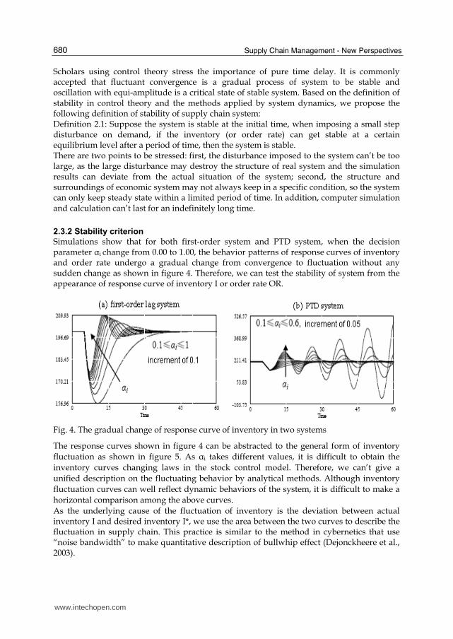
Simulations show that for both first-order system and PTD system, when the decision parameter αi change from 0.00 to 1.00, the behavior patterns of response curves of inventory and order rate undergo a gradual change from convergence to fluctuation without any sudden change as shown in figure 4. Therefore, we can test the stability of system from the appearance of response curve of inventory I or order rate OR.

Fig. 4. The gradual change of response curve of inventory in two systems

The response curves shown in figure 4 can be abstracted to the general form of inventory

fluctuation as shown in figure 5. As αi takes different values, it is difficult to obtain the

inventory curves changing laws in the stock control model. Therefore, we can’t give a

unified description on the fluctuating behavior by analytical methods. Although inventory

fluctuation curves can well reflect dynamic behaviors of the system, it is difficult to make a

horizontal comparison among the above curves.

As the underlying cause of the fluctuation of inventory is the deviation between actual inventory I and desired inventory I*, we use the area between the two curves to describe the fluctuation in supply chain. This practice is similar to the method in cybernetics that use “noise bandwidth” to make quantitative description of bullwhip effect (Dejonckheere et al., 2003).

www.intechopen.com


Fig. 5. The general behavior pattern of inventory fluctuation

As shown in figure 5, assuming that the inventory curve begins to fluctuate at time t0, the

inventory curve and desired inventory level intersect at time t1, t2…ti…tn in succession, and

the area between two curves can be divided into several parts S1，S2…Si...Sn. Let the

absolute value of the area between the two curves be sn，that is:

sn=∑ |S辿|辿退樽辿退怠 (10)

i. If the system is smooth convergence, then there is only one arc between the two curves:

sn = |S1| (11)

ii. If the system is fluctuant convergence, then |Si| > |Si+1| (i=1,2…n). There exists a natural number N, when t ≥ tN, I ≡ I*,|SN+1| ≈ 0, and:

lim樽→袋著 s樽 = s択 = ∑ |S辿| = C樽辿退怠 (Constant) (12)

iii. If the system is oscillation with equi-amplitude, then |S1|=|S2|=…=|Si| =…=|Sn|, and:

sn=∑ |S辿| = n|S怠|樽辿退怠 (13)

iv. If the system is divergent fluctuation, then |Si| < |Si+1| (i=1,2…n) and:

lim樽→袋著 s樽 = 髪∞ (14)

To sum up, that is:

完 |I岫t岻 − I∗|dt = ∑ |S辿| = s樽樽辿退怠担投担轍 (15)

S岫t樽岻 = 完 |I岫t岻 − I∗|dt担投担轍 (16)

where S is the inventory integral curve. We can distinguish the behavior of the system according to the form of curve S, that is, S curve can be used as the stability criterion of the system.

www.intechopen.com


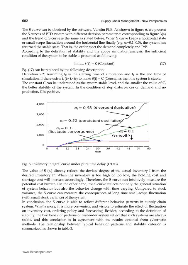
The S curve can be obtained by the software, Vensim PLE. As shown in figure 6, we present the S curves of PTD system with different decision parameter αi corresponding to figure 3(a) and the trend of S curve is the same as stated before. When S curve keeps a horizontal state or small-scope fluctuation around the horizontal line finally (e.g. αi=0.1; 0.3), the system has returned the stable state. That is, the order meet the demand completely and I=I*. According to the definition of stability and the above simulation analysis, the sufficient condition of the system to be stable is presented as following:

lim担→著 S岫t岻 = C (Constant) (17) Eq. (17) can be replaced by the following description: Definition 2.2: Assuming t0 is the starting time of simulation and tF is the end time of simulation, if there exists ts (t0≤ts≤tF) to make S(t) = C (Constant), then the system is stable. The constant C can be understood as the system stable level, and the smaller the value of C, the better stability of the system. In the condition of step disturbances on demand and no prediction, C is positive.

Fig. 6. Inventory integral curve under pure time delay (DT=3)

The value of S (tn) directly reflects the deviate degree of the actual inventory I from the

desired inventory I*. When the inventory is too high or too low, the holding cost and

shortage cost will increase accordingly. Therefore, the S curve can intuitively measure the

potential cost burden. On the other hand, the S curve reflects not only the general situation

of system behavior but also the behavior change with time varying. Compared to stock

variance, the S curve can measure the consequences of long time small-scope fluctuation

(with small stock variance) of the system.

In conclusion, the S curve is able to reflect different behavior patterns in supply chain

system. What’s more, it is more convenient and visible to estimate the effect of fluctuation

on inventory cost, ordering policy and forecasting. Besides, according to the definition of

stability, the two behavior patterns of first-order system reflect that such systems are always

stable, and this conclusion is in agreement with the results obtained from cybernetic

methods. The relationship between typical behavior patterns and stability criterion is

summarized as shown in table 2.

www.intechopen.com


Inventory status Sharp of S curve Delay mode System state

Smooth convergence Be similar to exponential curve, base number∈(0.-1)

First-order; PTD

Stable

Fluctuant convergence Be similar to exponential curve, base number∈(0.-1)

First-order; PTD

Stable

Oscillation with equi-amplitude

Be similar to straight line PTD Critical stable

Divergent fluctuation Be similar to exponential curve, Base number∈(1,+∞)

PTD Unstable

Table 2. Behavior pattern and its stability

3. Study on the stability of general inventory control system

In the last section, the dynamic characteristics of single parameter stock control system were discussed and we adopt the inventory integral curve as the criterion for stability judgment. Based on cybernetic studies, the dynamic behavior patterns of inventory in supply chain system are limited to the four typical behavior patterns shown in table 2 (Lalwani et al., 2006). Therefore, as a result of primary judge, the stability criterion proposed in the previous section is still valid for more complicated systems. However, the single parameter stock control model has ignored the management of WIP and there is significant difference between theoretical model and managerial practice. Meanwhile, the previous simulation shows that the delay structure of WIP is a key factor of system stability. Therefore, it is of great theoretical and practical importance to study the effect of WIP on stability of supply chain system. In this section, based on the generic stock-management model (Riddalls＆Bennett, 2002;

Sterman, 1989), we add the WIP control loop to the previous model and built a general inventory control system with dual-loop and double decision parameters. Then the applicability of stability criterion is validated and the stability characteristics in double parameters control model with two different delay structures are discussed.

3.1 General inventory control system model 3.1.1 Basic assumptions

The general inventory control system model in this section can be still understood as one node along the chain, the basic assumptions are the same as i-iv described in 2.1.1. Considering the management of WIP, assumption v in 2.1.1 is changed as following: v.The supply chain members adjust orders according to demand from downstream, actual storage and WIP, and maintain the inventory at a desired level.

3.1.2 Structure of the model

Figure 7 represents the general inventory control model: Compared to the model in figure 1, there are three increasing variables: WIP* the desired WIP, AWIP the adjustment for WIP, ALPHAwip (αWIP) the rate at which the discrepancy between actual and desired WIP levels is eliminated, 0≤αWIP≤1,

www.intechopen.com


Fig. 7. The general inventory control model

3.1.3 Variable settings

Except the indicated orders, the settings of other variables in inventory control loop are the

same as Eq. (2)-(6). To regulate WIP, a negative feedback mechanism is used. Adjustments

are then made to correct discrepancies between the desired and actual inventory AI, and

between the desired and actual WIP AWIP. Eq. (1) is adjusted as follows:

IO = D + AI + AWIP (18)

Since WIP* is proportional to the demand as well as the delay time, we define the desired WIP as the delay time multiplied by the demand D. That is

WIP* = D×DT (19)

AWIP=αWIP (WIP*-WIP) (20)

WIP* reflects the excepted value of future delivery situation. For production-oriented

enterprises, WIP* reflects the supply capacity of upstream raw materials and production

capacity on the node; for distribution firms, WIP* reflects the channel capacity between two

nodes. In fact, there are multiple ways to measure WIP* and Eq. (19) adopts the linear

approximation method. As this chapter focuses on structure factors, when imposing small

disturbance on the system, the estimate precision of WIP* has little influence on the system

stability.

According to Eq. (6) and Eq. (20), the ordering policy is defined below:

IO = D + αi (I* - I) + αWIP (WIP* - WIP) (21)

This ordering policy is still based on the anchoring and adjustment heuristic. Compared to

Eq. (7), Eq. (21) considers two anchoring points, that is, I* and WIP*. The ordering policy is

one of the dual parameter decision rules. When αWIP=0, figure 6 is equivalent to figure 1.

Therefore, the general inventory control model covers the single parameter stock control

model.

www.intechopen.com


3.2 Dynamic characteristics analysis of system 3.2.1 Simulation design

Except the parameters involved in WIP, the initial values of the variables are the same as

presented in 2.2.1. For the convenience of comparison, we set the value of αWIP to zero, that

is, the initial state of the model is equivalent to single parameter stock control model. We still adopt the small disturbance for stability examination, and the demand function is unchanged:

D = D担轍(1+STEP (0.2, 5)) (22)

In the presence of small disturbance, the decision parameter αi is changed from 1 to 0 with a

small decrement Δi. At the same time, αWIP varies from 0 to 1 with another small increment

ΔWIP, the smaller the values of Δi and ΔWIP, the higher the simulation accuracy. The process can be described by pseudo-code below:

For (αi =1; αi≥0; αi =αi -Δi)

{ for (αWIP =0; αWIP≤1; αWIP =αWIP +ΔWIP)

{ Run Model }

}

This section focuses on the interaction of dual-loop and verifying the applicability of

stability criterion proposed in the previous section to general inventory control system.

Through simulation, we can observe the behavior patterns of general inventory control

system and test the system stability in the situation of complete rationality (αi, αWIP∈[0,1]),

then the simulation results can be compared with that of single parameter stock control

model.

3.2.2 Dynamics characteristics of system

1. First-order system The first-order lag is described as Eq. (8). If αWIP=0, the general inventory control model is equivalent to single parameter stock control model. From the previous analysis, when αi changes continuously, the response curves of inventory I* and desired rate OR can always converge to a stable state. There are only two typical behavior patterns: smooth convergence and fluctuant convergence.

If αWIP≠0, when αi takes a particular value andαWIP varies from 0 to 1 with a small increment

ΔWIP, the shapes of response curves of inventory I* and desired rate OR are still restricted

to the above mentioned two typical behavior patterns. The nearer αWIP approaches 1, the

more obvious the smoothness of response curves will be. The nearer αWIP approaches 0, the

more obvious the fluctuation characteristics of response curves will be. Figure 8 shows the

response curves of inventory of the general inventory control system under first-order lag

when DT=3 and αi=0.4.

Together with figure 2, it leads to the conclusion that the general inventory control system

under first-order lag is usually stable, but αWIP and αi have exerted totally different influence

on the dynamics characteristics of system. This conclusion also hold in the case when delay

www.intechopen.com


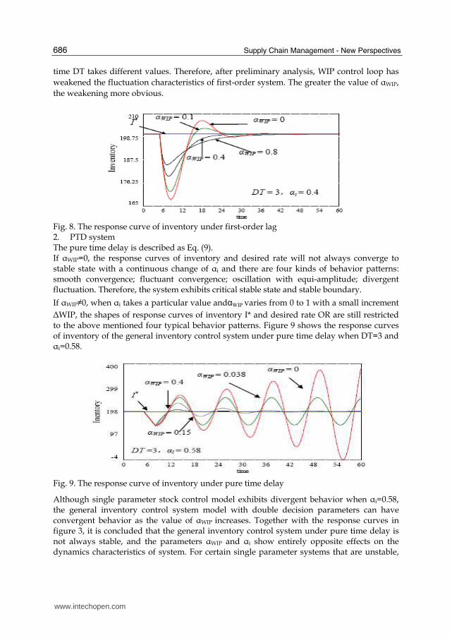
time DT takes different values. Therefore, after preliminary analysis, WIP control loop has

weakened the fluctuation characteristics of first-order system. The greater the value of αWIP,

the weakening more obvious.

Fig. 8. The response curve of inventory under first-order lag 2. PTD system The pure time delay is described as Eq. (9). If αWIP=0, the response curves of inventory and desired rate will not always converge to stable state with a continuous change of αi and there are four kinds of behavior patterns: smooth convergence; fluctuant convergence; oscillation with equi-amplitude; divergent fluctuation. Therefore, the system exhibits critical stable state and stable boundary.

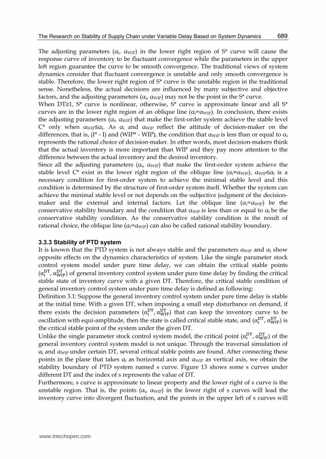
If αWIP≠0, when αi takes a particular value andαWIP varies from 0 to 1 with a small increment

ΔWIP, the shapes of response curves of inventory I* and desired rate OR are still restricted to the above mentioned four typical behavior patterns. Figure 9 shows the response curves of inventory of the general inventory control system under pure time delay when DT=3 and αi=0.58.

Fig. 9. The response curve of inventory under pure time delay

Although single parameter stock control model exhibits divergent behavior when αi=0.58, the general inventory control system model with double decision parameters can have convergent behavior as the value of αWIP increases. Together with the response curves in figure 3, it is concluded that the general inventory control system under pure time delay is not always stable, and the parameters αWIP and αi show entirely opposite effects on the dynamics characteristics of system. For certain single parameter systems that are unstable,

www.intechopen.com


by adding decision parameter αWIP and enhancing WIP control loop, the systems can reach stable state. Thus, WIP control loop has also weakened the fluctuation characteristics of PTD system.

3.3 Stability analysis of general inventory control system

3.3.1 Stability criterion

Following definition 2.1, the inventory integral curve is used as the stability criterion of supply chain system. This stability criterion can be generalized to the general inventory control system model with double decision parameters only when the following conditions are satisfied: First, the response curve of inventory I (or order rate OR) is limited to the range listed in table 2; Second, the response curve of inventory I (or order rate OR) is gradually changing as the decision parameters αWIP and αi change, and there is no mutation in this process. As the WIP control loop has in fact weakened the fluctuation characteristics of single parameter system model, the behavior patterns of general inventory control model will not go beyond that of single parameter stock control model. Therefore, the behavior patterns of system listed in table 2 still apply to general inventory control system model. Figure 10 shows the traverse of the response curve of inventory under different delay modes. Through the analysis of figure 4, figure 8 and figure9, the increased αi will increase the fluctuation while the increased αWIP will cushion the fluctuation both in first-order system and PTD system after disturbed, and the processes are smooth. Together with figure 10, the system hasn’t appeared other new behavior patterns and mutation points.

Fig. 10. The traverse graph of inventory curves of general inventory control system model

In conclusion, the dynamic patterns and stability criterion obtained from the analysis of single parameter stock control system model still hold in the general inventory control system model under first-order lag and pure time delay.

3.3.2 Stability of first-order system

This research indicates that the first-order system is always stable and the two decision parameters have different effects on system stability. Figure 8 shows that the system stability is increasing with the increase of αWIP. Similarly, we obtain the S curve of the general inventory control system model under first-order lag (see figure 11). According to

www.intechopen.com


definition 2.2, the constant C represents the stable level of system. Figure 11 shows that the value of C will decrease when increasing αWIP under the condition of the given delay time and αi. But there exists a minimum C*, when the system achieves C*, increase of αWIP won’t help improve system stability. Let C* be the minimal stable level which is determined by αi with a given DT, αWIP, then determines whether the system can achieve the stable level C* or not. Before the system achieves the stable level C*, the response curve of inventory appears to be fluctuant convergence, but when the system has achieved the stable level C*, the response curve of inventory tends to be smooth convergence, and the increase of αWIP can only reduce the deviation between actual inventory I and desired inventory I* and postpone the stabilizing time of the system.

Fig. 11. Inventory integral curve of general inventory control model under first-order lag

Further analysis indicates that there is an exclusive αWIP corresponding to αi (αi, αWIP∈[0,1]) to make the system achieve the stable level C*. Based on the analysis, the minimal stability boundary of general inventory control model under first-order lag with different DT is obtained as shown in figure 12 (x-axis is αi, y-axis is αWIP). We use S* curve to express the minimal stability boundary, each point on the curve can guarantee that the system will achieve the stable level C*.As shown in figure 12, the index of S* represents the value of DT.

Fig. 12. The minimal stability boundaries of first-order system under different DT

www.intechopen.com


The adjusting parameters (αi, αWIP) in the lower right region of S* curve will cause the response curve of inventory to be fluctuant convergence while the parameters in the upper left region guarantee the curve to be smooth convergence. The traditional views of system dynamics consider that fluctuant convergence is unstable and only smooth convergence is stable. Therefore, the lower right region of S* curve is the unstable region in the traditional sense. Nonetheless, the actual decisions are influenced by many subjective and objective factors, and the adjusting parameters (αi, αWIP) may not be the point in the S* curve. When DT≥1, S* curve is nonlinear, otherwise, S* curve is approximate linear and all S* curves are in the lower right region of an oblique line (αi=αWIP). In conclusion, there exists the adjusting parameters (αi, αWIP) that make the first-order system achieve the stable level C* only when αWIP≤αi. As αi and αWIP reflect the attitude of decision-maker on the differences, that is, (I* - I) and (WIP* - WIP), the condition that αWIP is less than or equal to αi

represents the rational choice of decision-maker. In other words, most decision-makers think that the actual inventory is more important than WIP and they pay more attention to the difference between the actual inventory and the desired inventory. Since all the adjusting parameters (αi, αWIP) that make the first-order system achieve the stable level C* exist in the lower right region of the oblique line (αi=αWIP), αWIP≤αi is a necessary condition for first-order system to achieve the minimal stable level and this condition is determined by the structure of first-order system itself. Whether the system can achieve the minimal stable level or not depends on the subjective judgment of the decision-maker and the external and internal factors. Let the oblique line (αi=αWIP) be the conservative stability boundary and the condition that αWIP is less than or equal to αi be the conservative stability condition. As the conservative stability condition is the result of rational choice, the oblique line (αi=αWIP) can also be called rational stability boundary.

3.3.3 Stability of PTD system

It is known that the PTD system is not always stable and the parameters αWIP and αi show

opposite effects on the dynamics characteristics of system. Like the single parameter stock

control system model under pure time delay, we can obtain the critical stable points

(α辿第鐸,α茸瀧沢第鐸 ) of general inventory control system under pure time delay by finding the critical

stable state of inventory curve with a given DT. Therefore, the critical stable condition of

general inventory control system under pure time delay is defined as following:

Definition 3.1: Suppose the general inventory control system under pure time delay is stable

at the initial time. With a given DT, when imposing a small step disturbance on demand, if

there exists the decision parameters (α辿第鐸,α茸瀧沢第鐸 ) that can keep the inventory curve to be

oscillation with equi-amplitude, then the state is called critical stable state, and (α辿第鐸,α茸瀧沢第鐸 ) is

the critical stable point of the system under the given DT.

Unlike the single parameter stock control system model, the critical point (α辿第鐸,α茸瀧沢第鐸 ) of the

general inventory control system model is not unique. Through the traversal simulation of

αi and αWIP under certain DT, several critical stable points are found. After connecting these

points in the plane that takes αi as horizontal axis and αWIP as vertical axis, we obtain the

stability boundary of PTD system named s curve. Figure 13 shows some s curves under

different DT and the index of s represents the value of DT.

Furthermore, s curve is approximate to linear property and the lower right of s curve is the

unstable region. That is, the points (αi, αWIP) in the lower right of s curves will lead the

inventory curve into divergent fluctuation, and the points in the upper left of s curves will

www.intechopen.com


make the inventory curve convergent. As DT increases, s curve tends to converge toward

the oblique line: αWIP=αi/2. Simulations show that the oblique line (αWIP=αi/2) is the upper

bound when s curve moves up to top left with DT increasing. Thus, it can be concluded that

the upper left area of oblique line (αWIP=αi/2) is the stable region which is independent of

delay (IoD), and the oblique line (αWIP=αi/2) is defined as IoD stability boundary of PTD

system. Since the models of supply chain in this research take no account of predictions, the

conclusions above not only validate the results obtained by cybernetic method from the

point of view of system dynamics, but also prove that IoD stability boundary is only

determined by systemic structure.

Fig. 13. The stability boundaries of PTD system under different DT

Meanwhile, there also exists a minimal stability boundary of PTD system under the given DT. The minimal stability boundaries of PTD system under different DT are shown in figure 13. The simulation results show that the greater the DT value, the more obvious the linearity of s* curve, when DT≥9, s* curve and the oblique line (αWIP=αi) nearly coincide. Similarly, αWIP≤αi is also the necessary condition for PTD system to achieve the minimal stable level and the oblique line (αi=αWIP) is the conservative stability boundary or rational stability boundary of PTD system.

3.3.4 Discussion

The main difference between the general inventory control model and the single parameter stock control model are the WIP control loop and the ordering strategy. The single parameter decision rule is marked IO1 and the two-parameter decision rule is marked IO2, that is:

IO1 = D + αi(I* - I) (22)

IO2 = D + αi(I* - I) + αWIP(WIP* - WIP) (23)

As compared with Eq. (22), Eq. (23) contains the new WIP adjustment. From the static perspective, IO2 is greater than or equal to IO1 under the same initial conditions and the demand will be enlarged. But through the dynamic methods, it is found that the two-

www.intechopen.com


parameter decision rule actually restraints the demand amplification and reduces the fluctuation of inventory and order rate because of the WIP control loop. Some studies on stability of supply chain based on dynamic methods suggest that the increase in αWIP and decrease in αi can contribute to improving the stability of the system (Disney et al., 2004; Riddalls et al., 2000; Sterman, 1989), but the findings of this section indicate that the above policies are effective only in the lower right region of the minimal stability boundary s* curve. Second, neither first-order system nor PTD system has the same rational stability boundary. This rational boundary conforms well to the results of beer game (Sterman, 1989). Although Sterman adopted first-order lag as the delay mode when modeling the beer game, the participants hadn’t known the delay mode and they didn’t estimate the delay mode of WIP control loop. Therefore, the conservative stability boundary or rational stability boundary actually has nothing to do with delay. Finally, the minimal stable level C* proposed in this section is relevant to the convergence properties of inventory fluctuation, it can’t guarantee the minimum cost. From the point of view of cost optimizing, there also exists an optimal boundary which depends on the ability of inventory management and the composition of inventory cost.

4. Conclusions

To conduct quantitative analysis on the stability of supply chain system with Order-Up-To (OUT) policy, we first built the single parameter stock control model of supply chain. By simulation analysis, a system-dynamics-based criterion for stability judgment is proposed. With simulation, the criterion can be used to describe the nonlinearities of supply chain system with 1st order exponential lag and pure time delay (PTD).The criterion can also be used to judge the influences exerted on supply chain stability by decision behavior. The simulation demonstrates two different results. Firstly, the 1st order system is usually stable, but there is fork effect as decision parameter changes. Secondly, there is a critical stable bound in PTD system, which determines the feasible filed of decision. Then a general inventory control system model is proposed. The model is provided with two typical delay modes: fist-order exponential delay and pure time delay. According to the concept of stability and stability criterion proposed in the previous section, stability borders with different meanings are confirmed, which integrate the results derived from different research methods. It is concluded that the stability of inventory control system is mainly decided by the features of feedback systems, the subjective decision and environment take their effects based on the feedback systems, and information sharing is propitious to increase the stability and weaken bullwhip effect of supply chain system. This research adopts the method of system dynamics and takes the delay modes as key point to discuss stability of supply chain system. Although preliminary achievements have been made, further research needs to be done on the stability of supply chain. With the development of research, we wish this chapter will contribute to supply chain management theories and practices.

5. References

Bertrand, J.W.M. (1980). Analysis of a production-inventory control system for a diffusion

department. International Journal of System Science, Vol.11, No.5, pp. 589-606.

www.intechopen.com


Bertrand J.W.M. (1986). Balancing production level variations and inventory variations in

complex production systems. International Journal of Production Research, Vol.24,

No.5, pp. 1059-1074.

Croson R. & Donohue K. (2005). Upstream versus downstream information and its impact

on the bullwhip effect. System Dynamics Review, Vol.21, pp. 249-260.

Daganzo C.F. (2004). On the Stability of Supply Chains. Operations Research, Vol.52, No.6, pp.

909-921.

Dejonckheere J., Disney S. M., & Lambrecht, M. R. et al. (2003). Measuring and avoiding the

bullwhip effect: A control theoretic approach. European Journal of Operational

Research, Vol.147, No.3, pp. 567-590.

Deziel, D. P. & Eilon, S. (1967). A linear production - inventory control rule. The Production

Engineer, Vol. 43, pp. 93-104.

Disney S.M. & Towill D.R. (2002). A discrete transfer function model to determine the

dynamic stability of a vendor managed inventory supply chain. International

Journal of Production Research, Vol. 40, No.1, pp.179-204.

Disney, S.M. & Towill, D.R. (2003a). On the bullwhip and inventory variance produced by

an ordering policy. The International Journal of Management Science, Vol.31, No.3, pp.

157-167.

Disney S.M. & Towill D.R. (2003b). The effect of Vendor Managed Inventory dynamics on

the Bullwhip Effect in supply chains. International Journal of Production Economics,

Vol.85, pp. 199-215.

Disney S.M., Towill D.R. & Van De Velde W. (2004). Variance amplification and the golden

ratio in production and inventory control. International Journal of Production

Economics, Vol.90, No.3, pp. 295-309.

Disney S.M., Towill D.R. & Warburton R.D.H. (2006). On the equivalence of control

theoretic, differential, and difference equation approaches to modeling supply

chains. International Journal of Production Economics, Vol.10, pp. 194-208.

Forrester J.W. (1958). Industrial dynamics: a major breakthrough for decision makers.

Harvard Business Review, Vol.36, No.4, pp. 37–66.

Forrester J.W. (1961). Industrial Dynamics. Cambridge: MIT Press, ISBN 978-1883-823-36-8,

Cambridge, UK.

Geary S., Disney S. M. & Towill D. R. (2006). On bullwhip in supply chains: historical

review, present practice and expected future impact. International Journal of

Production Economics, Vol. 101, pp.2-18.

Holweg M & Disney S.M. (2005). The evolving frontiers of the bullwhip effect. Proceedings of

the EurOMA 2005 Conference, pp. 707-716, Budapest, Hungary, June 19-22,2005.

Huixin Liu, Hongwei Wang & Qi Fei. (2004). Stability analysis for an inventory control

system. Computer Integrated Manufacturing Systems. Vol.10, No.11, pp.1396-1401.

Jing Wang, Haiyan Sun & Yilan Li. (2006).Irregular information distortion and weakening

methods in supply chains. Journal of Beijing University of Aeronautics and

Astronautics.Vol.32, No. 12, pp. 1481-1484.

Lalwani C.S., Disney S.M. & Towill D.R. (2006). Controllable, observable and stable state

space representations of a generalized order-up-to policy. International Journal of

Production Economics, Vol.101, pp.172-184.

www.intechopen.com


Larsen E.L., Morecroft J.D.W. &Thomsen J.S. (1999). Complex behaviour in a production

distribution model. European Journal of Operational Research, Vol.119, No.1,

pp.61-74.

Lee H.L., Padmanabhan V. & Whang S. (1997a). Information distortion in a supply chain:

The bullwhip effect. Management Science, Vol.43, pp.546-558.

Lee H.L., Padmanabhan V. & Whang S. (1997b). The Bullwhip Effect in Supply Chains. Sloan

Management Science, Vol.38, pp.93-102.

Magee J. (1958). Production Planning and Inventory Control. McGraw-Hill, ISBN 0205081479,

New York, London.

Miragliotta G. (2006). Layers and mechanisms: A new taxonomy for the Bullwhip Effect.

International Journal of Production Economics, Vol.104, No. 2, pp.365-381.

Naim M.M. & Towill D.R. (1995). What is in the pipeline?. Proceedings of 2nd International

Symposium on Logistics, pp.135-142, Nottingham, UK, July 11-12,1995.

Ouyang F. & Daganzo C.F. (2006). Characterization of the Bullwhip Effect in Linear, Time-

Invariant Supply Chains: Some Formulae and Tests. Management Science, Vol.52,

No.10, pp.1544-1556.

Qifan Wang. (1995). Advanced System Dynamics. Tsinghua University Press. ISBN 7-302-

01838-3, Beijing.

Riddalls C.E. & Bennett S. (2001). Optimal control of batched production and its effect on

demand amplification. International Journal of Production Economics, Vol.72, pp. 159-

168.

Riddalls C.E. & Bennett S. (2002). The stability of supply chains. International Journal of

Production Research, Vol.40, pp.459-475.

Riddalls C.E., Bennett S. & Tipi N.S. (2000). Modelling the dynamics of supply chains.

International Journal of System Science, Vol.31, No.8, pp. 969-976.

Simon, H. A. (1952). On the application of servomechanism theory to the study of

production control. Econometrica, Vol.20, pp.247-268.

Sterman J.D. (1989). Modeling Managerial Behavior: Misperceptions of feedback in a

dynamic decision making experiment. Management Science, Vol.35, No.3, pp. 321-

339.

Sterman J. D. (2000). Business Dynamics: Systems Thinking and Modeling for a Complex World.

McGraw-Hill/Irwin, ISBN 0072311355, New York.

Taylor, D.H. (1999). Measurement and analysis of demand amplification across the supply

chain. International Journal of Logistics Management, Vol.10, pp. 55–70.

Towill D.R. (1982). Dynamic analysis of an inventory and order based production

control system. International Journal of Production Research, Vol.20, No.6, pp.

671–687.

Towill D.R. (1996). Industrial dynamics modelling of supply chains. Logistics Information

Management, Vol.9, No.4, pp.43-56.

Tversky, A. & D. Kahneman. (1974). Judgment under uncertainty: heuristics and biases.

Science, Vol.185, pp. 1124-1131.

Vassian H.J. (1955). Application of discrete variable servo theory to inventory control.

Journal of the Operations Research Society of America, Vol.3, No.3: 272-282.

www.intechopen.com


Xinan Ma, Lieping Zhang & Peng Tian. (2005). Delay in a supply chain. System Engineering.

Vol.5, pp. 97-102.

Zhang X. (2004). The impact of forecasting methods on the Bullwhip Effect. International

Journal of Production Economics, Vol.88, pp.15-27.

www.intechopen.com

Supply Chain Management - New PerspectivesEdited by Prof. Sanda Renko

ISBN 978-953-307-633-1Hard cover, 770 pagesPublisher InTechPublished online 29, August, 2011Published in print edition August, 2011

InTech EuropeUniversity Campus STeP Ri Slavka Krautzeka 83/A 51000 Rijeka, Croatia Phone: +385 (51) 770 447 Fax: +385 (51) 686 166www.intechopen.com

InTech ChinaUnit 405, Office Block, Hotel Equatorial Shanghai No.65, Yan An Road (West), Shanghai, 200040, China

Phone: +86-21-62489820 Fax: +86-21-62489821

Over the past few decades the rapid spread of information and knowledge, the increasing expectations ofcustomers and stakeholders, intensified competition, and searching for superior performance and low costs atthe same time have made supply chain a critical management area. Since supply chain is the network oforganizations that are involved in moving materials, documents and information through on their journey frominitial suppliers to final customers, it encompasses a number of key flows: physical flow of materials, flows ofinformation, and tangible and intangible resources which enable supply chain members to operate effectively.This book gives an up-to-date view of supply chain, emphasizing current trends and developments in the areaof supply chain management.

How to referenceIn order to correctly reference this scholarly work, feel free to copy and paste the following:

Suling Jia, Lin Wang and Chang Luo (2011). The Research on Stability of Supply Chain under Variable DelayBased on System Dynamics, Supply Chain Management - New Perspectives, Prof. Sanda Renko (Ed.), ISBN:978-953-307-633-1, InTech, Available from: http://www.intechopen.com/books/supply-chain-management-new-perspectives/the-research-on-stability-of-supply-chain-under-variable-delay-based-on-system-dynamics

© 2011 The Author(s). Licensee IntechOpen. This chapter is distributedunder the terms of the Creative Commons Attribution-NonCommercial-ShareAlike-3.0 License, which permits use, distribution and reproduction fornon-commercial purposes, provided the original is properly cited andderivative works building on this content are distributed under the samelicense.

https://creativecommons.org/licenses/by-nc-sa/3.0/

the research on stability of supply chain under variable

Documents