The research program of the Center for Economic Studiesproduces a wide range of theoretical and empirical economicanalyses which serve to improve the statistical programs of theU.S. Bureau of the Census. Many of these analyses take the formof research papers. The purpose of the Discussion Papers is tocirculate intermediate and final results of this research amonginterested readers within and outside the Census Bureau. Theopinions and conclusions expressed in the papers are those of theauthors and do not necessarily represent those of the U.S. Bureauof the Census. All papers are screened to ensure that they donot disclose confidential information. Persons who wish toobtain a copy of the paper, submit comments about the paper, orobtain general information about the series should contact SangV. Nguyen, Editor, Discussion Papers, Center for EconomicStudies, Room 1587, FB 3, U.S. Bureau of the Census, Washington,DC 20233(301-763-2065).

PUBLISHED VERSUS SAMPLE STATISTICS FROM THE ASM:

IMPLICATIONS FOR THE LRD

by

Steve J. Davis*

John Haltiwanger**

Scott Schuh***

CES 91-1 January 1991

Abstract

In principle, the Longitudinal Research Database (LRD) whichlinks the establishments in the Annual Survey of Manufactures (ASM)is ideal for examining the dynamics of firm and aggregate behavior.However, the published ASM aggregates are not simply theappropriately weighted sums of establishment data in the LRD.Instead, the published data equal the sum of LRD-based sampleestimates and nonsample estimates. The latter reflect adjustmentsrelated to sampling error and the imputation of small-establishmentdata. Differences between the LRD and the ASM raise questions forusers of both data sets. For ASM users, time-series variation inthe difference indicates potential problems in consistently andreliably estimating the nonsample portion of the ASM. For LRDusers, potential sample selection problems arise due to thesystematic exclusion of data from small establishments.Microeconomic studies based on the LRD can yield misleadinginferences to the extent that small establishments behavedifferently. Similarly, new economic aggregates constructed fromthe LRD can yield incorrect estimates of levels and growth rates.This paper documents cross-sectional and time-series differencesbetween ASM and LRD estimates of levels and growth rates of totalemployment, and compares them with employment estimates provided byBureau of Labor Statistics and County Business Patterns data. Inaddition, this paper explores potential adjustments to economicaggregates constructed from the LRD. In particular, the paperreports the results of adjusting LRD-based estimates of gross jobcreation and destruction to be consistent with net job changesimplied by the published ASM figures.

Keywords: Longitudinal data, Annual Survey of Manufactures, grossjob flows

*Graduate School of Business, University of Chicago**Department of Economics, University of Maryland***Department of Economics, Johns Hopkins University and Center forEconomic Studies, Bureau of the Census

In preparing this study, we have benefited from the comments andassistance of Robert Bechtold, Stacey Cole, Tim Dunne, Easley Hoy,David Lilien, Robert McGuckin, Jim Monahan and other Census Bureauemployees in the Center for Economic Studies and the IndustryDivision. We gratefully acknowlege research support provided by

the National Science Foundation and a Joint Statistical Agreementbetween the Census Bureau and the University of Maryland.

1

I. Introduction

The Longitudinal Research Database (LRD) maintained by the

Center for Economic Studies at the U.S. Bureau of the Census is a

vital source of annual and quarterly data on the manufacturing

sector between 1972 and 1986. By linking successive Annual Surveys

of Manufactures (ASM) at the establishment level, the LRD affords

a unique opportunity to study the time-series behavior of a large,

national probability sample of manufacturing establishments. The

LRD has been used to study mergers (McGuckin, Nguyen, and Andrews

1990), diversification (Streitwieser 1990), productivity

(Lichtenberg & Siegel 1990), and firm growth (Dunne, Roberts,

Samuelson 1989a, 1989b, and Pakes and Olley 1990). Moreover, the

LRD includes sample weights that, in principle, allow estimation of

new industry and sector aggregates that exploit the longitudinal

establishment linkages. Davis and Haltiwanger (1989,1990) exploit

these linkages to measure and study annual and quarterly gross job

flows.

Despite broad coverage, the LRD does not sample the entire

manufacturing universe. The ASM estimates published by the Census

Bureau (hereafter, published or ASM) equal the sum of nonsample

estimates and LRD-based sample estimates. The nonsample portion of

the published ASM figures reflect adjustments related to sampling

error and the imputation of small-establishment data. These

nonsample components of the published ASM figures have previously

been unavailable to LRD users. Although the LRD data are by far

the largest component of the ASM figures, marked cross-sectional

and time-series differences exist between the ASM and LRD.

Differences between the ASM and LRD raise questions for users

of both data sets. For ASM users, time-series variation in the

difference indicates potential problems in consistently and

reliably estimating the nonsample portion of the ASM. For LRD

2

users, potential sample selection problems arise. Since the

nonsample component of the ASM primarily reflects the behavior of

very small establishments, systematic differences between movements

in the sample and nonsample components presumably reflect

differences in the behavior of large and small plants. Thus,

microeconomic studies based on the LRD can yield misleading

inferences to the extent that small establishments behave

differently and are systematically excluded from the sample. By

the same token, new economic aggregates constructed from the LRD

can yield incorrect estimates of levels and growth rates.

This paper documents cross-sectional and time-series

differences between ASM and LRD estimates of levels and growth

rates of total employment, and compares them with employment

estimates provided by Bureau of Labor Statistics (BLS) and County

Business Patterns (CBP) data. For total manufacturing, employment

level and growth rate estimates display a high degree of similarity

across all four data sources. Similarities diminish markedly for

two- and four-digit industries dominated by small establishments.

In addition, the correspondence between the ASM and LRD

deteriorated after 1979, when ASM sampling procedures changed.

Perhaps most troublesome, discrete changes in the divergence

between ASM and LRD-based estimates occur in the first year of each

panel and in census years. This pattern reflects cumulative multi-

year employment changes that are first reflected in the published

ASM figures in census years and first reflected in the LRD at the

commencement of a new five-year panel. Although ASM figures

typically correspond more closely to BLS and CBP figures, the LRD

appears to provide superior growth rate estimates in certain years.

In any case, further analysis of ASM-LRD differences seems

warranted.

Beyond documenting ASM-LRD differences, this paper explores

potential adjustments to economic aggregates constructed from the

LRD. In particular, the paper reports the results of adjusting the

3

LRD-based estimates of gross job creation and destruction

calculated by Davis and Haltiwanger (1989, 1990) to be consistent

with the net job changes implied by published ASM figures. LRD-

based estimates of gross job flows represent lower bounds on true

(ASM) gross job flows, because they fail to capture job creation

and destruction among manufacturing establishments outside the

sampling frame of the LRD. A more important concern regarding the

LRD-based measures of gross job flows is that, by neglecting the

behavior of very small establishments, they possibly provide a

distorted picture of time-series and cross-sectoral patterns of

covariation between gross job creation and gross job destruction.

In practice, the adjustment of LRD-based gross job flow

measures for consistency with the ASM measure of net job flows

raises difficult problems. This paper implements and evaluates a

simple methodology that treats the difference between the ASM and

LRD at the four-digit level of disaggregation as a pseudo-

establishment. Job creation and destruction among pseudo-

establishments are calculated and added to the LRD-based figures to

obtain adjusted gross flows. This procedure understates true gross

flows from the nonsample portion of the ASM but potentially

improves upon the unadjusted measures. Unfortunately, in census

years and in the first year of each panel, the nonsample portion

exhibits discrete employment changes that distort adjustments to

the gross flows. In other years, the adjustment procedure appears

to work well but have little impact.

We draw two conclusions from our adjustment exercise. First,

the simple adjustment procedure yields estimates of gross job flow

rates that are inferior to their counterparts based solely on the

LRD. Second, we find no evidence that inferences based on the

time-series properties of the LRD-based gross job flow measures

are distorted by a sampling frame that excludes very small

establishments.

4

II. ASM Sampling Procedure

A. LRD Background

The LRD is a comprehensive collection of establishment-level

economic data on U.S. manufacturing firms between 1972 and 1986.

The annual portion contains about 860,000 observations on 160,000

plants on many aspects of production: shipments, employment,

capital expenditures and assets, raw material inputs, inventories,

payroll, and many other variables. The LRD also contains detailed

classification data such as geography, industry, ownership, and

plant type. For details of the LRD's specific contents, see

McGuckin and Pascoe (1989).

The annual portion of the LRD comprises the linked sample data

from the ASM. Conducted since 1949, the survey tracks for five

years a panel of establishments selected from a size-weighted

probability sample. Sampled establishments represent about

one-sixth of manufacturing plants and three-fourths of employment.

The sampling frame encompasses all but the smallest establishments,

typically those with five or fewer employees. Large establishments

are sampled with certainty. A new panel of establishments is

selected in years ending in 4 and 9 (e.g., 1974, 1979) from the

universe of manufacturing establishments identified by the

quinquennial Census of Manufactures (CM), which occurs in years

ending in 2 and 7 (e.g., 1982, 1987). The annual LRD contains four

panels: 1969-73, 1974-78, 1979-83, and 1984-88. (Data for 1969-71

are not available; data for 1987 and later years will be added as

they become available.) New establishments are added to ongoing

panels to incorporate births and preserve the representative

character of the panel.

B. Published ASM Estimates

Published aggregate ASM statistics reflect additional

5

X A(st) ' X L(st) % X F(st) % X I(st) , (1)

information beyond that contained in the LRD. In particular, the

published data include two additive adjustments representing

sampling error and small-establishment imputation. Let X represent

an ASM data item (in this paper X is total employment). Then

published ASM X is

where the superscript A denotes ASM, L denotes LRD, F denotes

fixed-base difference (sampling error), I denotes imputed data, s

refers to sector (e.g., industry), and refers to time (year). The

empirical section shows that these two nonsample components, though

small relative to the sample component, can be important influences

on the published levels and growth rates.

During the period covered by the LRD, the methodology used to

estimate the components of equation (1) underwent significant

changes, thereby affecting the relationship between the published

ASM and sample LRD data. To understand the behavior of these

components, it is important to understand the development of the

ASM sampling procedure, so the remainder of this section describes

each component in more detail. Complete descriptions of these

sampling issues can be found in Ogus and Clark (1971) and Waite and

Cole (1980).

C. Sample Estimates

In selecting an ASM sample of establishments from the CM

universe, the Census Bureau uses a sampling technique that defines

independent sampling units and uses a probability proportional to

size (PPS) method to assign selection probabilities to each unit.

These probabilities are independent of the selection outcome of all

other sampling units or groups of units. A linear unbiased

6

X L(st) ' ju

W(ut) X L(ust) , (2)

estimate of, for example, total employment of all sampling units

(u) at time t is

where W(ut), the sample weight, is the reciprocal of the sampling

probability. A sampling probability of 0.25 implies a sample

weight of 4 and the sampling unit's data represents that of four

units. The variance of the estimate (2) is minimized when the

selection probability is a constant fraction of sampling unit size.

In principle, a separate selection probability should be assigned

for each data item, but, in practice, a common size measure

determines the sample weight for all data items. The current size

measure for the ASM weights is total value of shipments within a

product class. An advantage of this sampling procedure is the

independence of selection probabilities because it permits

arbitrary assignment of certain probabilities, such as one (certain

inclusion) for large establishments.

Two significant changes in the sample selection procedure

occurred during the LRD period. The first change pertained to the

definition of the sampling unit. Before 1979, the company (the

group of establishments legally attached to a single manufacturing

organization) served as the sampling unit. If a company was

selected (using probabilities derived from company size), then all

establishments belonging to that company were included in the

panel. Since 1979, however, the establishment has been the

sampling unit. Only establishments selected (using probabilities

derived from establishment size) are included in the panel. The

Bureau switched to an establishment-based sampling scheme because

it requires fewer establishments to achieve the same estimation

efficiency.

The second major sampling change altered the nature of the

7

sample weights. Since 1963, the CM has excused certain very small

single-unit (SU) establishments from completing the survey to

reduce respondent burden (i.e, they were given sample weights of

zero). During the LRD period these establishments, known as

administrative records (ARs), represented about one- third of the

total manufacturing universe of approximately 350,000

establishments. From 1972-78, the sample weights generated for the

remaining non-AR establishments took account of the existence of

the AR establishments, in which case (2) is a suitable estimate of

the aggregate quantity. Beginning in 1979, however, the sample

weights did not account for AR establishments, and so it became

necessary to independently estimate AR establishment data and add

it to the weighted sample estimate (2). This independent estimate

is the imputed component of (1) and is described in the next

subsection.

To maintain the representativeness of the sample, the Census

Bureau adds births of new establishments to the panel each year.

Three types of establishments are added to a panel. Multi-unit

births are identified from the Bureau's annual Company Organization

Survey (COS), in which multi-unit companies describe their

organizational status. Single-unit births are identified from

periodic listings of Social Security Administration (SSA) issues of

new Employer Identification (EI) numbers. (Since many births are

very small or related to non- ASM companies, not all are added to

the panel.) Finally, during the company-based survey period, many

establishments were added due to corporate reorganization.

Timing difficulties arise regarding births. Nearly all births

appear in the ASM panel for the first time in the year following

the actual birth year. Consequently, both ASM and LRD estimates

reflect measurement errors generated by the mistiming of births.

Davis and Haltiwanger (1989, 1990) discuss procedures for adjusting

the employment data to address this problem. By focusing on March

total employment in the analysis below, the extent of timing

8

X F(st) ' ji 0 CM(s,t&2)

X L(is,t&2) & ji 0 ASM(st)

W(ist) X L(is,t&2) (3)

mismeasurement is mitigated, because births that occur after March

12 are properly timed with respect to March employment figures.

(There are related but less severe difficulties for deaths; see

Davis and Haltiwanger (1989,1990)).

D. Nonsample Estimates

Two nonsample components also enter into the published ASM

estimates. These nonsample estimates are: 1) constant (within

panel) estimates of the sampling error called the fixed-base

difference (FBD); and 2) imputed data for the ARs and births not

included in the panel, a total called the impute (or small) block

(IB).

The FBD represents an adjustment of the LRD estimates for

sampling error using estimates from the most recent previous CM.

The FBD is

for the period t representing the first year of a panel. CM(st)

and ASM(st) denote the sample of establishments in the respective

survey. The FBD remains at this level through the third year of

the panel. (In the fourth panel year, the CM estimate is used in

generating the published ASM figure.) If the panel-based weighted

estimates equaled the CM figure, the FBD would be zero (abstracting

from the impute block). Minimizing the FBD is one panel selection

criterion. Notice that during the panel another CM occurs so that

any error accumulated during the first three panel years is

eliminated by recalculating the FBD. This recalculation is done

and applied to the fifth panel year sample estimate analogously to

(3).

The imputed estimates for establishments outside the panel

(ARs and small births) are derived from payroll and employment

9

information obtained by the Bureau from IRS data. For each

impute-block establishment, the Bureau receives March total

employment and quarterly payroll (PAY) information from which it

imputes estimates of all other CM data items. Next, the

impute-block employment and payroll data are tabulated to

four-digit SIC industry by state by metropolitan statistical area

(MSA) cells. Then the imputed data for that cell is

10

X I(st) '

ji0ASM(st)

X L(ist)

ji0ASM(st)

PAY L(ist)j

i0IB(st)PAY(ist)I . (4)

TE ' j4

q'1

PW(q)/4 % OE , (5)

TE ' PW(1) % OE (6)

That is, the imputed value of the data item equals the industry

average ratio of the item to payroll times cell payroll.

III. Empirical Evidence

A. Data Description

The data will be described using the following notation: A

stands for ASM, L for LRD, D for the difference A-L, F for FBD, and

I for IB, B for BLS, and C for CBP. In census years the CM

estimate is the published number but for simplicity we use ASM (A).

Exceptions are noted. The variables used are total employment

(TE), production worker employment (PW), and other employment (OE).

Sector and time subscripts are suppressed unless necessary for

expositional clarity.

Because the definitions and timing of employment vary across

data sources, it is necessary to consider different types and

periods of employment measures. ASM and LRD quarterly PW estimates

represent employment on the 12th of March, May, August, and

November, and OE is collected for March 12. Annual TE is

where q indexes quarters. March LRD TE is

11

ITE d ' ATE & LTE & FTE . (7)

Since published ASM data do not include an analogue of (6), we

estimate published ASM March TE by multiplying annual ASM TE by the

ratio of annual ASM TE to annual LRD TE.

The CBP data are only available for March, and BLS March

employment is that observed from the monthly establishment survey

data. (An annual BLS analogue of (5) can be calculated.) The BLS

data also contain the employment of auxiliary manufacturing

establishments, which are owned by and support manufacturing

enterprises but are not directly involved in manufacturing. The

ASM, LRD, and CBP data exclude auxiliary establishments, whose

employment amounts to approximately one million. We concentrate on

the March employment data in the remainder of this section.

Historical FBD and IB data are not included in the LRD data.

In principle, it is possible to use the LRD and CM data available

at the Center for Economic Studies to recreate the FBD using

equation (3) and derive the IB (impute block) from 1979 forward

using the formula ITE=ATE- LTE-FTE. Attempts to execute this

procedure have been unsuccessful thus far, though we are still

investigating the problem.

Fortunately, we obtained unpublished industry level FBD and IB

data on actual FTE and ITE for 1982, 1983, and 1984. Given the

constancy of FTE, a derived ITE, ITEd, for 1979 to 1986 may be

calculated from the formula

There are thus two versions of the difference between ASM and LRD

employment:

12

DTE ' FTE % ITE d

DTE( ' FTE % ITE , (8)

where ITE=ITEd in the missing years, 1979-81 and 1985-86.

B. Comparisons of Levels and Growth Rates

Figures 1 and 2 plot the level and growth rate of total

manufacturing employment estimated via a number of different

methods and sources. The plots indicate that published ASM and LRD

sample estimates follow the same basic time-series pattern.

However, three sources of divergence stand out. First, the

divergence between the levels of the ASM and the LRD estimates are

much larger after 1979. This change reflects the effects of the

switch to an establishment-based sample frame in 1979 and the

tendency of ITE to grow over time. The effect of the change on

growth rates is much less pronounced.

Second, there is a deterioration in the correspondence between

the LRD and ASM that occurs within each panel. This is evidenced

by a growing divergence in the levels within each panel and a sharp

divergence in the growth rates between the ASM and the LRD in the

first year of each panel. The latter reflects the correction

incorporated into the LRD from the cumulative divergence that

occurred in the previous panel.

Third, there is an increased divergence between the published

and LRD levels and growth rates in census years (1977 and 1982).

This is due to a cumulative intercensus distortion. Recall that

published estimates reflect the entire manufacturing universe in

census years. Accordingly, in census years reported one-year

changes reflect cumulative changes since the previous census that

were not previously incorporated into the published ASM figures.

Comparison with other data sources indicates that all of the

estimates follow the same basic pattern in both levels and growth

rates. BLS employment levels are higher for the entire period,

reflecting the inclusion of auxiliary administrative

13

establishments. The ASM estimates track the CBP and BLS estimates

better than do the LRD estimates.

Quantitative evidence on growth rates for total manufacturing

and 2-digit industries is presented in Table 1 (total manufacturing

in this and all succeeding tables is denoted as industry 00).

Several patterns emerge from Table 1. For total manufacturing, the

mean growth rates across the published, weighted sample, BLS, and

CBP measures are reasonably similar in magnitude, and the

time-series standard deviations are highly similar. Thus, the

table confirms the basic message of Figure 1 that, in terms of

growth rates for total manufacturing, ASM-LRD differences are

small.

There is considerable heterogeneity across industries in terms

of the differences among published ASM, LRD, BLS, and CBP estimates

of growth rates. Since small establishments dominate the behavior

of the nonsample portion of the ASM, an obvious source of

heterogeneity is differences in the size distribution of

establishments. The mean establishment size is reported in the

rightmost column of Table 1. For industries in which the

establishment mean is relatively large (e.g., SIC 21-Tobacco, SIC

33-Primary Metals, SIC 37-Transportation Equipment), the mean and

standard deviation of growth rates from the ASM and LRD are very

similar. In contrast, for industries in which the establishment

mean is relatively small (e.g., SIC 24-Lumber, SIC 27-Printing, SIC

39-Miscellaneous), the differences between the ASM and LRD growth

rates in terms of means and/or standard deviations are large.

Time-series correlations of the employment growth rate

estimates are reported in Table 2. For total manufacturing, the

time-series pairwise correlations across all of the alternative

growth rate series is quite high. However, the correlations

between the ASM and either BLS or CBP are slightly higher than the

correlations between the LRD and either BLS or CBP.

The diversity across industries in means and standard

14

deviations indicated in Table 1 carries over to the correlations,

shown in Table 2. Again, the industry size distribution is

important. Industries dominated by large establishments (e.g., 33

and 37) have very high pairwise correlations. Industries dominated

by smaller establishments (e.g.,20, 27, and 39) have substantially

lower pairwise correlations, especially between the LRD and the

ASM.

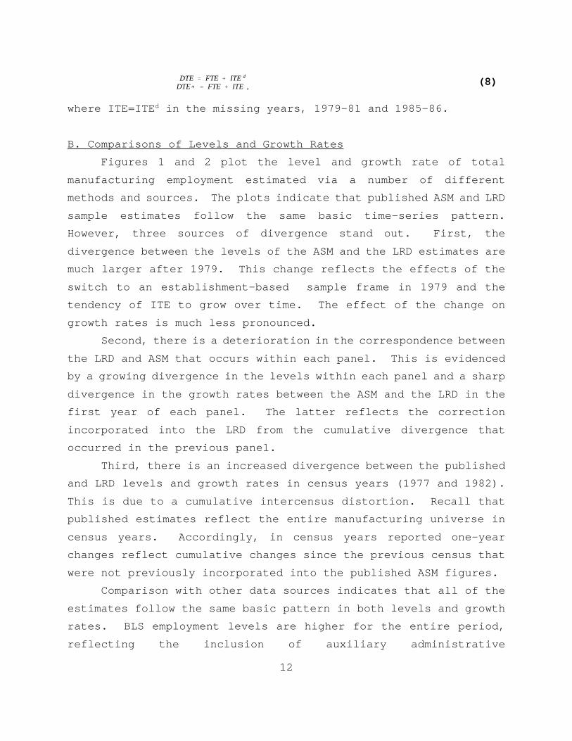
Figures 3 and 4 depict the substantial heterogeneity across

industries. For Primary Metals (33), the time-series pattern of

growth rates across the ASM, LRD, BLS and CBP is very similar. In

contrast, for Food (20) there are sharp differences in the patterns

of growth rates, especially between the LRD and the ASM.

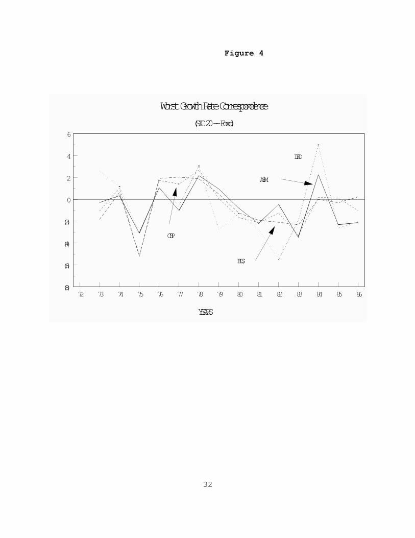
While there is considerable diversity across industries, for

most industries there is a high correlation between the LRD and ASM

growth rates. This can be clearly seen from Figure 5 which plots

a histogram of the correlations between LRD and ASM growth rates by

4-digit industry. The vast majority of 4- digit industries have a

correlation in excess of 0.70. The non- trivial minority of

4-digit industries with low correlations are industries that

present researchers with potentially severe sample selection

problems.

As is apparent from Figure 1, the nature of the divergence

between the ASM and the LRD varies across panels. Table 3 presents

means and standard deviations of growth rates for the 1974-78 panel

and the 1979-83 panel. Two observations stand out from Table 3.

First, even for total manufacturing, the LRD estimates deviate

substantially from the ASM

and other estimates to a far greater extent during the 1979-83

panel than during the 1974-78 panel. Second, even for industries

characterized by small establishments (e.g, 27), the

divergence between the LRD estimates and the ASM estimates is

relatively small for the 1974-78 period. These comparisons of

levels and growth rates highlight several messages that emerge from

15

this analysis. First, the correspondence between the behavior of

the LRD and ASM estimates is reasonably high for total

manufacturing and very high for industries dominated by large

establishments. Second, the correspondence between the LRD and ASM

is better prior to 1979. Third, discrete changes in the divergence

between the ASM and the LRD occur in the first year of each panel

and in census years. Both of the latter effects reflect cumulative

five-year changes that are concentrated in those respective years.

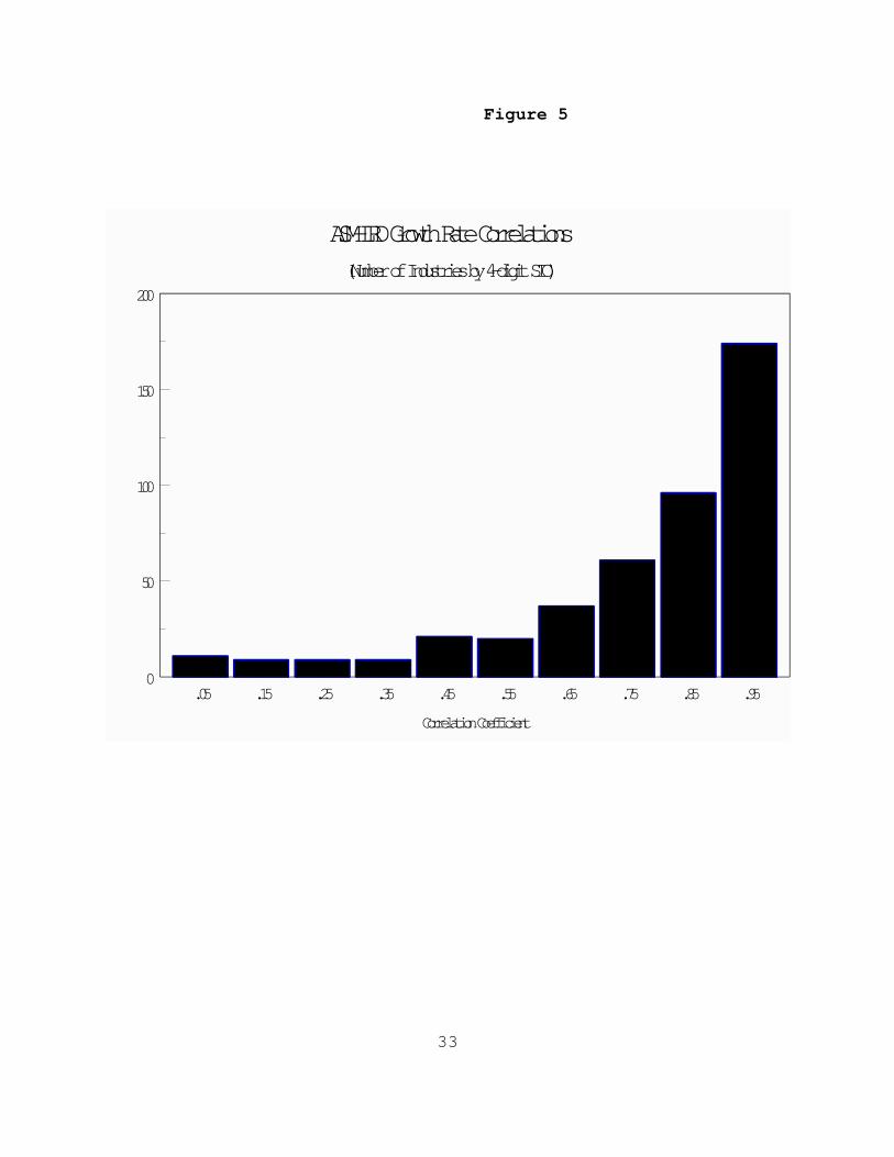
C. Decomposition of ASM Estimate

The behavior of the difference (DTE) between LTE and ATE is by

construction driven by the behavior of FTE and ITEd (or ITE). This

section analyzes the decomposition of ATE in terms of its three

true components, LTE, FTE, and ITE, rather than using ITEd. Since

FTE and ITE data are only available since 1979, we accordingly

focus on the 1979-86 period.

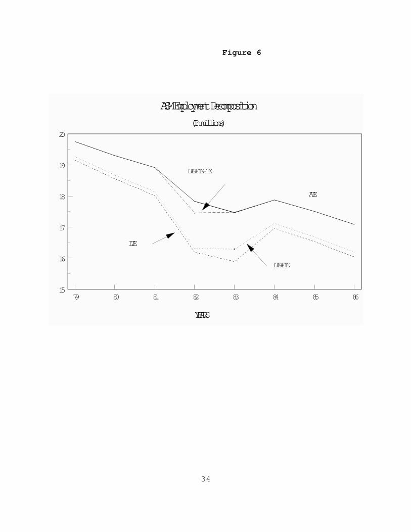
Figure 6 plots the decomposition of ATE between 1979 and 1986.

From 1979 to 1981, the difference between ATE and LTE grows very

slightly. In 1982, the difference between ATE and LTE increases

discretely. The difference between ATE and LTE remains large in

1983 and then falls substantially in 1984. From 1984 to 1986 the

difference is relatively constant. The basic pattern is that the

difference is relatively constant except

in census years and in the first year of each panel.

Figure 7 shows that the most striking feature of DTE behavior

is the discrete jump in 1982. Moreover, it is clear that much of

the increase cannot be attributed to either an increase in ITE or

FTE. This apparent contradiction of the identity linking the three

components of ATE is reflected in the distinction between DTE and

DTE*. The latter represents what the difference in 1982 would have

been if the published total had simply reflected the sum of the

three components, LTE, FTE and ITE. However, published totals in

16

a census year are based on the census totals rather than the sum of

the three components. In 1982, we see that there is a large

discrepancy between the sum of the three components and the census

total.The other discrete change in DTE occurs in 1984. DTE drops

substantially from 1983 to 1984. This decrease is attributable to

a decline in both ITE and FTE between 1983 and 1984. This discrete

change reflects the change in panels between 1983 and 1984.

Additional quantitative evidence on the relationship between

the components of ATE is provided in Table 4. The striking finding

from Table 4 is that while the growth rate correlation between ATE

and LTE is quite high for total manufacturing and most 2-digit

industries, the correlation between ATE and ATE* is surprisingly

low. ATE* represents the sum of LTE, FTE and ITE, which equals

ATE except in 1982-1984. The discrepancy in these years is

apparently large enough to drive the correlation between the growth

rates of ATE and ATE* down substantially.

These results suggest that the discrete changes observed in

published estimates in census years are due to factors other than

discrete changes in FTE and ITE. Apparently, published totals in

census years incorporate changes that have occurred between

censuses but have not been reflected in the intervening published

ASM estimates. These changes come from the discovery of births not

identified in the prior five years, more accurate estimation of AR

data, reclassification of nonmanufacturing establishments as

manufacturing, and other sources. This implies that while census-

year levels are undoubtedly accurate, estimating one-year changes

from the difference between a census-year published total and a

previous-year published total is apt to generate a biased estimate

of the change. This raises doubts about how to interpret the time

series behavior of ATE over intervals that include census years.

In contrast to the discrete change in 1982, the discrete

change in DTE in 1984 does not raise questions about estimating

changes from published ASM estimates. Rather, the discrete change

17

in 1984 reflects a change in the relative importance of each of the

components of ATE, with DTE becoming smaller and LTE becoming

larger. This does, however, suggest that estimates of changes

using LRD estimates are apt to be particularly unreliable in the

first year of each panel. Similarly, using changes in DTE to

represent changes in the behavior of AR cases and small births is

apt to be unreliable in the first year of each panel. Both of

these latter problems cause difficulties in developing procedures

for adjusting LRD estimates to be consistent with published totals

(as will become apparent in the next section).

D. Summary of Basic Findings

A summary of the relationship between ASM and LRD estimates is

illustrated in Figure 8, which depicts the simplified development

of a hypothetical ASM panel. In most years, the levels and growth

rates of employment are more accurately estimated by the published

ASM data. Exceptions to this conclusion follow.

In terms of employment levels, the sample LRD data are never

superior to the published ASM data. In the first panel year the

two estimates are the closest, but the sample LRD data deviate from

the published data by a small FBD and (from 1979 forward) an impute

block, which is at its smallest value. As the panel progresses,

the sample LRD employment level increasingly deviates from the

published ASM data (exhibited by the different slopes) because the

impute block is growing and because the weighted sample estimate

becomes biased over time. The latter effect occurs as

establishment sizes change over time. Notice that the published

ASM employment level is also biased and requires the large

adjustment that occurs in the census year. This bias may come from

births not detected between CMs, for example.

In terms of growth rates, the published ASM and sample LRD

estimates are likely to be very similar in the second, third, and

fifth panel years. However, the ASM estimate is preferable in the

18

first year and the LRD estimate in the fourth (census) year for

related reasons. In the census year, the ASM (CM) estimate jumps

discretely, imposing the cumulative (undetected) changes from the

previous four years. This potentially large growth rate probably

overstates the true change, which the LRD -- because it doesn't

impose the correction -- more accurately captures. The reverse

occurs in the first panel year. The selection of a new panel, new

sample weights, new IB, and new FBD discretely adjust the sample

LRD level, causing a large and likely biased growth rate estimate.

The first panel year problem with the sample LRD growth rate seems

to be empirically larger than that for the published ASM data in

the census year.

IV. Application to Gross Employment Flows

A. Motivation for Measuring Gross Flows

Considerable attention in both the data and research community

has been devoted to estimating and studying gross worker flows

across labor market states (i.e., employment, unemployment, not in

the labor force, etc.). While these flows are clearly of interest,

it is equally important to estimate and analyze gross job flows.

In the absence of evidence from longitudinal establishment data on

gross job flows, it has been difficult to determine whether

observed large gross worker flows primarily reflect temporary

layoffs and recalls plus continual sorting and resorting of workers

across a given set of jobs, or alternatively, whether a large

portion of worker turnover reflects gross job reallocation across

establishments.

The LRD is well-suited to the measurement of high frequency

19

POS ' ji 0 E%

x(i)X

g(i) (9)

(annual and quarterly) gross job flows. The LRD allows for careful

treatment of births and deaths so that spurious entry and exit due

to ownership change and other forms of reorganization can be

controlled for. Further, the LRD provides detailed information

that permits estimation of gross job flows across numerous key

establishment characteristics. As such, the LRD offers substantial

advantages over alternative data sources that can be used for this

purpose (see, e.g., Leonard (1987), Birch (1981), and Armington and

Odle (1982)).

Davis and Haltiwanger (1989,1990) report research on the

cyclical properties and implications of gross job creation and

destruction using gross job flows estimated from the LRD. In these

studies, the impact of the nonsample portion of the ASM on gross

job flows is neglected. In what follows, the role of the nonsample

portion of the ASM on gross job flows is investigated. Procedures

for incorporating the nonsample portion in gross job flow estimates

are discussed and a crude version of these procedures is

implemented. In the analysis, the focus is on annual gross job

flows but the issues and procedures discussed apply to the

quarterly job flow estimates as well.

B. Gross Job Creation and Destruction

The measures of gross job creation and destruction used here

are those of Davis and Haltiwanger (1989, 1990). Creation is the

sum of all new jobs in expanding establishments and destruction the

sum of all lost jobs at contracting establishments. Expressed as

rates relative to sector size, these measures are

20

NEG ' ji 0 E&

x(i)X

*g(i)* , (10)

NET ' POS & NEG . (11)

SUM ' POS % NEG . (12)

where g(i) is the growth rate of establishment i at t, E+ is the

set of establishments with positive and E- with negative growth

rates, , x(i) is establishment size, and X is sector size. Size is

measured as the average of employment at time t and t-1, i.e.,

x(it) = 0.5(x(it) + x(i,t-1)), and g(it) is the change in

establishment employment divided by establishment size.

POS and NEG represent lower bounds on total creation and

destruction because individual jobs within establishments cannot be

distinguished. Thus a net establishment level job change of zero

may include creation and destruction that merely alters the

composition of types of jobs within establishments. To interpret

POS and NEG, note that net employment growth is

Hence, POS and NEG represent the gross changes across

establishments that underlie the observed net change. A summary

measure of gross job reallocation is

There are numerous interpretations of SUM. First, X times SUM

represents the gross change in the number of employment positions

at establishments. Second, X times SUM is an upper bound on the

number of workers who must switch jobs and/or employment status to

accommodate the redistribution of employment positions across

establishments. Third, SUM is the size-weighted mean absolute

deviation of establishment growth rates around zero. Accordingly,

21

it has a formal statistical interpretation as a measure of

dispersion.

C. Measurement Methodology

To obtain empirical estimates of the creation, destruction,

and reallocation measures from the LRD, it is necessary to

calculate creation and destruction for each establishment at each

time t. If measured employment in the current and prior years are

both positive, measurement proceeds as in (9) and (10). But, if

measured employment is positive in one year but zero in the other,

then additional information is used to determine whether a true

birth or death occurred. For the purposes of computing POS, a

birth is recorded only if the establishment had zero employment in

prior years of the panel and if the LRD coverage code, which

provides information on organizational changes, indicates that a

new establishment is born. Likewise, for the purposes of computing

NEG, a death is recorded only if the establishment had an

appropriate coverage code.

The reselection of a new panel of ASM establishments every

five years generates difficulties in measuring gross flows in the

first year of each panel. Since only about one-third of the

establishments in the previous panel continue into the current

panel, simple calculation of gross employment change will

mistakenly overestimate the change by attributing panel entry and

exit to creation and destruction. However, information on gross

job creation and destruction for continuing establishments across

panels can be used to impute total gross job creation and

destruction for the first period of each panel. An imputation

based upon simple bivariate regressions is used in the results that

follow. Since the imputation used is crude, considerable caution

should be used in interpreting results for 1974, 1979 and 1984.

D. Adjusting the Gross Flows

22

POS ( ' ji 0 E% ^D%

x(i)X

g(i) (13)

In Davis and Haltiwanger (1989,1990) the creation and

destruction measures were calculated using only the sample portion

(i.e., LRD) of the data that underlie the published ASM figures.

In principle, it is desirable to incorporate the nonsample portion

of the ASM into the estimates of the gross flows. However, in

practice, there are numerous difficulties given the nature of the

nonsample portion of the ASM and the discrete changes in the

nonsample portion that occur in census years and the first year of

each panel.

Unfortunately, establishment-level data for the nonsample

portion of the ASM are unavailable. The nonsample portion of the

estimate is available at the four-digit level of disaggregation.

Given this limitation, we implement a simple procedure for

adjusting the LRD-based gross flows to incorporate information on

the nonsample portion of the ASM. Essentially, the nonsample

portion of each four-digit industry is treated as a

pseudo-establishment. That is, the entire difference between

published ASM and LRD estimates, DTE, is the pseudo-establishment

from which additional creation or destruction can be calculated to

add to the LRD based measures. Using this pseudo-establishment

method, the adjusted (*) POS and NEG are

23

NEG ( ' ji 0 E& ^D&

x(i)X

*g(i)* , (14)

where D+ (-) is the set of pseudo-establishments with growing

(shrinking) employment.

Treating the nonsample portion as a pseudo-establishment

generates gross flow estimates that are consistent with net changes

in the published ASM figures. However, this procedure understates

the gross flows associated with the nonsample portion, because net

changes at the four-digit level mask offsetting establishment-level

net changes within the nonsample portion of four-digit industries.

A second problem with this procedure is that the nonsample

portion of the ASM exhibits discrete changes in census years and in

the first year of each panel. These discrete changes will be

reflected in the adjustment of the gross flows and thus generate

distortions in those years.

An alternative to the pseudo-establishment method is to use

the information available from the LRD regarding the relationship

between gross and net flows for small establishments. This

relationship could be used to impute gross flows for the nonsample

portion based upon the actual net changes for the nonsample

portion. Further, an adjustment could be made in the census years

and the first year of each panel to spread the observed discrete

changes appropriately over the course of the panel. Development of

an imputation procedure along these lines will be considered in

future work.

E. Results Using the Pseudo-Establishment Method

The effect of using the pseudo-establishment method on total

manufacturing POS and NEG are shown in Figures 9 and 10. In years

other than census years and the first year of each panel, the

24

adjustment generates sensible results. The adjustment in such

years tends to increase POS and NEG but the magnitude of the

adjustment is marginal. For these years, means (standard

deviations) are: POS - 9.03% (0.033), POSA - 9.35% (0.031), NEG

- 11.15% (0.047), and NEGA - 11.26% (0.044).

In contrast, Figures 9 and 10 suggest that the discrete

changes in the nonsample estimates generate distorted adjustments

in census years and in the first year of each panel. Combined with

the results of section III, this pattern indicates that the method

fails to deliver a satisfactory adjustment in census years and in

the first year of each panel.

Additional evidence on the relationship between adjusted and

unadjusted gross flows appears in Table 5. Time-series

correlations of the adjusted and unadjusted series are reported,

excluding the first year of each panel and census years. For total

manufacturing, correlations between adjusted and unadjusted series

are quite high for POS, NEG, NET and SUM. The cross correlation

between POS and NEG for total manufacturing is negative and about

the same magnitude for adjusted and unadjusted series, and the same

holds for the negative cross correlation between NET and SUM.

The same general patterns hold for the two-digit industry

data. Not surprisingly, the adjusted and unadjusted series behave

very similarly for industries with primarily large establishments

(e.g., 33 and 37), while the series are less similar for industries

dominated by small establishments (e.g., 27 and 39). However, even

for the latter industries, the behavior of the adjusted and

unadjusted is quite similar.

Overall, this pseudo-establishment adjustment method works

reasonably well in years other than census years and the first year

of each panel. However, in such years, the adjustment makes little

difference to magnitudes or time-series properties of the gross

flows. For census years and the first year of each panel, the

current adjustment procedure is inappropriate. Since the

25

adjustment makes little difference in years in which it is

successful, these results supports the integrity of LRD-based

estimates of gross flows. Further, given the difficulties with the

adjustment procedure in other years, the LRD-based estimates of

gross flows are at present a more reliable, internally consistent

time series. Refinements to the adjustment procedure to

incorporate the nonsample portion must be developed before reliable

adjustments can be generated.

V. Conclusion

The imperfect relationship between published ASM and sample

LRD data has potentially important implications for researchers

using the LRD. LRD users should take this imperfect relationship

into account in the selection of industries, sectors and time

period of analysis.

Three main conclusions emerge with respect to the

time-series and cross-sectional characteristics of the published

ASM and sample LRD data. First, at high levels of aggregation

employment levels and growth rates generated from the two data sets

correspond closely. At the industry level, the quality of the

correspondence is high for industries dominated by large

establishments and lower for industries dominated by smaller

establishments. Second, the correspondence between published and

sample data deteriorates over the life of a panel due to sampling

and imputation errors. Third, the rotation scheme for ASM panels

leads to cumulative multi-year errors that show up in the published

figures during census years and in the LRD figures during the

first year of a new panel. The correction of cumulative errors

leads to a biased growth rate calculation in these years.

This paper also implemented an adjustment designed to

reconcile LRD-based estimates of gross job creation and destruction

26

with published ASM figures on net job changes. Our procedure, which

treats the ASM-LRD difference at the four-digit industry level as

a pseudo-establishment, proved unsatisfactory because of the

discrete changes in LRD and ASM employment figures associated with

corrections of cumulative estimation errors. These corrections

cause large changes in the ASM-LRD difference that induce spurious

movements in the adjusted gross job flow figures. We proposed two

alternative ways of handling these discrete changes in future

research. We conclude that there is no simple and satisfactory

method of reconciling the published and sample data.

27

References

Armington, Catherine and Marjorie Odle (1982), "Small Business --How Many Jobs?" Brookings Review, 1 (Winter), pp. 14-17.

Birch, David L. (1981), "Who Creates Jobs?" Public Interest, 65(Fall), pp. 3-14.

Davis, Steve J. and John Haltiwanger (1989), "Gross Job Creation,Gross Job Destruction, and Employment Reallocation," University ofMaryland Working Paper No. 89-31.

Davis, Steve J. and John Haltiwanger (1990), "Gross Job Creationand Gross Job Destruction: Microeconomic Evidence and MacroeconomicImplications," NBER Macro Annual 1990, forthcoming.

Dunne, Timothy, Mark J. Roberts, and Larry Samuelson (1989a), "TheGrowth and Failure of U.S. Manufacturing Plants," The QuarterlyJournal of Economics, Vol. 104, No. 4 (November), pp. 671-698.

Dunne, Timothy, Mark J. Roberts, and Larry Samuelson (1989b),"Plant Turnover and Gross Employment Flows in the U.S.Manufacturing Sector," Journal of Labor Economics, Vol. 7, No. 1(January), pp. 48-71.

Leonard, Jonathan (1987), "In the Wrong Place at the Wrong Time:The Extent of Frictional and Structural Unemployment," inUnemployment & the Structure of Labor Markets, Kevin Lang and J.Leonard eds., Basil Blackwell: New York.

Lichtenberg, Frank R. and Donald Siegel (1989), "Using LinkedCensus R&D-LRD Investment on Total Factor Productivity Growth,"Center for Economic Studies Working Paper No. 89-2.

McGuckin, Robert H. and George A. Pascoe, Jr. (1988), "TheLongitudinal Research Database: Status and Research Possibilities,"Survey of Current Business, Vol. 68, No. 11 (November), pp. 30-37.

McGuckin, Robert H., Sang V. Nguyen, and Stephen H. Andrews (1990),"The Relationships Among Aquiring and Acquired Firms' ProductLines," Working Paper.

Olley, G. Steven and Ariel S. Pakes (1990), "Dynamic BehavioralResponses in Longitudinal Data Sets: The TelecommunicationsEquipment Industry," Working Paper.

28

Ogus, Jack L. and Donald F. Clark (1971), The Annual Survey ofManufactures: A Report on Methodology, Technical Paper No. 24, U.S.Department of Commerce, Bureau of the Census.

Streitweiser, Mary L. (1990), "The Extent and Nature ofEstablishment Level Diversification in Sixteen U.S. ManufacturingIndustries," Working Paper.

Waite, Preston J. and Stacey J. Cole (1980), "Selection of a NewSample Panel for the Annual Survey of Manufactures," presented atthe annual meetings of the American Statistical Association,Houston, TX.

29

72 73 74 75 76 77 78 79 80 81 82 83 84 85 86

16

17

18

19

20

21

ASM

LRD

BLSCBP

Total Manufacturing Employment

(In millions)

YEARS

Figure 1

30

Employment Growth Rates

(March-to-March, Total Manufacturing)

72 73 74 75 76 77 78 79 80 81 82 83 84 85 86

(10)

(8)

(6)

(4)

(2)

0

2

4

6

8

10

ASMLRD

BLS

CBP

YEARS

Figure 2

31

Best Growth Rate Correspondence

(SIC 33 -- Primary Metals)

72 73 74 75 76 77 78 79 80 81 82 83 84 85 86(30)

(20)

(10)

0

10

20

ASM

LRD

BLS

CBP

YEARS

Figure 3

32

Worst Growth Rate Correspondence

(SIC 20 -- Food)

72 73 74 75 76 77 78 79 80 81 82 83 84 85 86(8)

(6)

(4)

(2)

0

2

4

6

ASM

LRD

BLS

CBP

YEARS

Figure 4

33

ASM-LRD Growth Rate Correlations(Number of Industries by 4-digit SIC)

.05 .15 .25 .35 .45 .55 .65 .75 .85 .950

50

100

150

200

Correlation Coefficient

Figure 5

34

ASM Employment Decomposition(In millions)

79 80 81 82 83 84 85 8615

16

17

18

19

20

ATE

LTE

LTE+FTE

LTE+FTE+ITE

YEARS

Figure 6

35

ASM-LRD Difference Decomposition(In millions)

79 80 81 82 83 84 85 860

0.5

1.0

1.5

2.0

DTE

FTE

ITE

DTE*

YEARS

Figure 7

36

Hypothetical ASM Panel

5 1 2 3 4 5 10

20

40

60

80

100

Census

FBD Adj.

Projected ASM Published Total

without Census FBD Adjustment

ATE

LTE

Inter-

Panel

Period

(IPP)

(IPP)

(Employment on the Vertical Axis)

PANEL YEARS

Figure 8

37

Adjusted vs. Unadjusted POS

(In rates)

73 74 75 76 77 78 79 80 81 82 83 84 85 860.06

0.08

0.1

0.12

0.14

0.16

POS*

POS

YEARS

Figure 9

38

Adjusted vs. Unadjusted NEG

(In rates)

73 74 75 76 77 78 79 80 81 82 83 84 85 860.04

0.06

0.08

0.1

0.12

0.14

0.16

0.18

NEG*

NEG

YEARS

Figure 10

39

Table 1

Average March-to-March Total Employment Growth Rates and Size, 1972-86(In percent)

ASM LRD BLS CBP SIZE MEANSSICCODE MEAN STD MEAN STD MEAN STD MEAN STD ESTAB COWKR

1 -0.13 4.70 -0.11 5.97 0.20 4.96 0.29 5.32 80 163120 -0.65 1.85 -0.70 2.89 -0.56 2.02 -0.61 2.10 82 47921 -2.09 3.65 -1.93 3.65 -1.39 3.28 -1.88 5.35 455 455222 -2.53 6.04 -2.27 7.07 -2.13 7.03 -2.20 6.08 156 85223 -1.88 5.74 -2.25 7.04 -1.29 6.70 -1.38 6.13 73 32124 -0.21 8.97 0.13 11.37 0.37 9.66 1.51 11.35 32 18225 0.49 7.37 0.90 9.76 0.70 8.36 0.69 8.15 68 45426 -0.23 4.15 -0.15 4.87 0.01 4.07 -0.06 3.81 117 52627 1.95 2.47 1.77 5.05 2.07 2.31 2.33 2.86 41 59328 -0.20 2.58 -0.38 3.06 0.20 2.53 -0.11 2.70 99 124329 -0.57 4.97 -0.44 5.46 -0.10 13.48 -0.65 3.20 81 85830 1.80 7.45 1.79 8.49 2.16 7.80 2.77 9.57 83 66231 -4.78 5.98 -4.16 6.70 -4.32 7.12 -4.59 6.72 101 35332 -1.04 5.04 -0.88 7.06 -0.75 6.18 -0.33 6.61 48 40933 -2.88 8.20 -2.80 8.96 -2.52 7.48 -2.77 8.10 176 293434 -0.01 5.81 0.06 7.47 -0.14 6.48 1.14 8.15 61 60535 0.60 7.25 0.65 8.82 1.23 7.68 1.11 8.07 65 135836 1.53 7.05 1.48 7.28 1.52 6.72 1.42 6.37 182 203237 0.52 6.20 0.57 6.67 1.15 6.49 0.68 6.81 283 659438 2.14 4.72 2.22 5.64 2.65 4.64 3.70 8.11 119 312339 -1.81 4.97 -1.54 8.08 -0.91 5.67 -0.44 6.97 41 337

40

Table 2

Total Employment Growth Rate Correlations, 1972-86

SIC (ATE, (ATE, (ATE, (LTE, (LTE, (BTE,CODE LTE) BTE) CTE) BTE) CTE) CTE)

1 0.93 0.96 0.96 0.91 0.91 0.9920 0.67 0.63 0.75 0.47 0.53 0.9521 0.87 0.64 0.83 0.36 0.77 0.5622 0.96 0.96 0.96 0.91 0.93 0.9823 0.86 0.85 0.84 0.82 0.81 0.9924 0.85 0.95 0.87 0.86 0.80 0.9125 0.93 0.94 0.92 0.91 0.87 0.9926 0.94 0.96 0.95 0.89 0.91 0.9727 0.27 0.73 0.68 0.38 0.32 0.8828 0.92 0.84 0.82 0.78 0.75 0.9829 0.82 0.70 0.45 0.65 0.34 0.1230 0.97 0.94 0.88 0.96 0.92 0.9531 0.92 0.89 0.94 0.82 0.86 0.9632 0.92 0.97 0.95 0.88 0.88 0.9833 0.99 0.98 0.97 0.96 0.96 0.9934 0.93 0.96 0.89 0.90 0.82 0.9335 0.95 0.97 0.98 0.94 0.94 0.9936 0.97 0.97 0.98 0.98 0.96 0.9837 0.98 0.96 0.99 0.98 0.99 0.9738 0.91 0.88 0.63 0.84 0.67 0.6939 0.63 0.80 0.68 0.81 0.69 0.94

41

Table 3

Average March-to-March Total Employment Growth Rates, 1974-1978(In percent)

ASM LRD BLS CBPSICCODE MEAN STD MEAN STD MEAN STD MEAN STD

1 0.55 6.39 0.33 6.35 0.31 6.98 0.46 7.0620 -0.23 2.33 0.11 2.61 0.16 3.55 0.14 3.6221 -3.03 0.56 -2.84 0.33 -2.09 2.36 -3.99 2.9522 -2.06 10.01 -2.69 9.69 -1.72 12.76 -1.99 10.5623 0.20 7.92 -0.66 7.51 -0.55 11.53 -0.42 10.5624 1.41 12.94 0.83 12.03 0.94 15.24 1.86 14.6025 1.16 11.82 0.60 11.45 0.48 14.18 0.64 14.4326 -0.39 7.17 -0.31 7.18 -0.29 7.42 0.34 6.6227 1.37 2.21 1.69 3.03 1.58 3.16 1.76 4.0728 0.86 2.74 1.00 2.37 0.80 3.40 0.79 4.1629 0.40 2.49 0.65 2.56 1.55 4.14 0.71 3.4130 3.12 12.34 2.73 12.25 2.30 12.30 2.46 11.8531 -1.44 7.81 -1.69 8.00 -1.44 12.33 -1.54 11.2632 -0.38 6.34 -0.11 6.70 -0.90 8.59 -0.89 8.8733 -2.39 5.57 -2.21 5.42 -1.72 5.48 -2.03 6.3034 0.59 7.70 1.05 8.16 0.31 8.25 0.81 8.5935 1.21 6.24 1.00 6.34 1.01 5.42 0.87 6.5136 1.15 11.30 0.34 10.88 0.10 10.16 0.41 10.1737 2.31 6.10 2.00 5.86 2.10 5.81 2.29 6.4838 3.18 5.68 2.17 5.39 2.18 6.14 3.31 4.6839 0.62 8.07 -1.24 7.88 -0.06 8.81 0.21 9.12

Average March-to-March Total Employment Growth Rates, 1979-1983

1 -3.41 2.22 -4.92 2.89 -3.79 2.25 -4.17 2.1120 -1.74 1.39 -2.88 1.85 -1.90 0.46 -2.09 0.8721 -1.65 5.57 -2.05 6.16 -0.10 3.40 -1.53 5.3922 -4.20 2.64 -5.32 3.90 -4.98 2.49 -5.15 2.2823 -2.92 2.25 -5.15 4.90 -3.78 0.86 -4.14 0.9024 -4.53 8.02 -7.27 9.73 -5.26 6.60 -5.91 6.7925 -2.85 2.66 -5.06 4.11 -3.94 1.73 -3.82 2.0226 -2.07 1.72 -2.72 2.46 -1.87 1.28 -2.36 2.0427 1.40 2.00 -0.52 2.43 1.13 1.18 0.70 1.5928 -1.26 2.97 -2.54 3.33 -1.31 2.33 -1.68 1.6729 -1.49 6.24 -3.30 6.62 1.21 27.21 -1.41 2.4930 -3.13 2.62 -4.96 1.39 -3.36 0.83 -4.79 1.4531 -5.64 3.14 -6.40 3.61 -4.85 2.57 -6.03 3.0832 -5.56 2.35 -7.15 4.08 -6.21 2.31 -6.00 2.4033 -10.6 6.71 -11.4 7.03 -9.97 6.64 -11.1 7.5034 -4.40 2.69 -6.18 3.09 -6.07 3.44 -5.58 2.7735 -4.57 7.33 -6.64 7.21 -5.00 8.65 -5.36 7.9236 -1.05 3.63 -1.74 3.43 -1.71 2.81 -1.27 3.86

42

37 -5.36 2.06 -6.16 2.68 -5.36 1.36 -6.21 1.8338 0.36 3.75 -1.04 3.10 0.26 3.97 -0.96 2.7739 -4.30 2.62 -8.02 4.49 -4.83 2.43 -5.42 3.05

1LTE=LTE; LTE*=LTE+FTE; ATE*=LTE+FTE+ITE; ATE=LTE+FTE+ITEd.

43

Table 4

Total Employment Growth Rate Correlations, 1979-861

SIC (ATE, (ATE, (ATE, (LTE, (LTE, (ATE*,CODE LTE) LTE*) ATE*) LTE*) ATE*) LTE*)

1 0.998 0.972 0.641 0.982 0.667 0.68220 0.205 -0.091 -0.273 0.942 0.168 0.21621 0.861 0.999 0.998 0.863 0.863 0.99722 0.920 0.980 0.984 0.956 0.867 0.94523 0.823 0.781 0.892 0.990 0.628 0.62924 0.926 0.968 0.687 0.986 0.566 0.62725 0.988 0.994 0.791 0.981 0.757 0.76626 0.956 0.998 0.796 0.970 0.827 0.78927 0.284 0.322 -0.075 0.989 -0.249 -0.33428 0.772 0.613 0.634 0.864 0.577 0.75829 0.258 0.569 0.794 0.552 0.315 0.90530 0.947 0.929 0.788 0.973 0.719 0.73231 0.790 0.958 0.905 0.910 0.752 0.91332 0.964 0.982 0.735 0.978 0.728 0.76033 0.997 0.997 0.994 0.997 0.994 0.99534 0.991 0.984 0.714 0.996 0.763 0.75235 0.943 0.914 0.800 0.988 0.801 0.77936 0.937 0.947 0.941 0.999 0.908 0.91837 0.987 0.994 0.987 0.984 0.973 0.99238 0.643 0.576 0.672 0.943 0.426 0.47939 0.395 0.644 0.663 0.854 0.153 0.387

44

Table 5

Correlations of Unadjusted and Adjusted Gross Flows, 1972-86(Excluding Census and First Panel Years)

Own Cross

(POS,NEG) (SUM,NET)SICCODE POS NEG SUM NET U A U A

1 0.981 0.978 0.956 0.985 -0.81 -0.72 -0.57 -0.4920 0.928 0.695 0.847 0.838 -0.31 0.10 0.05 0.2021 0.982 0.998 0.997 0.996 -0.79 -0.67 -0.50 -0.5122 0.985 0.980 0.978 0.983 -0.71 -0.65 -0.51 -0.4523 0.981 0.937 0.852 0.971 -0.73 -0.65 -0.17 0.1924 0.971 0.963 0.952 0.974 -0.75 -0.61 -0.22 -0.2725 0.988 0.944 0.948 0.964 -0.70 -0.61 -0.40 -0.3726 0.994 0.987 0.970 0.991 -0.85 -0.85 -0.72 -0.7127 0.936 0.770 0.862 0.920 -0.36 0.23 0.02 0.0128 0.661 0.974 0.841 0.916 -0.70 -0.44 -0.59 -0.5029 0.898 0.978 0.950 0.924 -0.33 -0.27 -0.24 0.0430 0.988 0.990 0.976 0.991 -0.88 -0.87 -0.58 -0.6331 0.975 0.991 0.997 0.989 -0.60 -0.41 -0.63 -0.6732 0.973 0.980 0.975 0.979 -0.55 -0.48 -0.45 -0.4133 0.997 0.998 0.997 0.999 -0.62 -0.57 -0.79 -0.7934 0.991 0.983 0.943 0.991 -0.84 -0.80 -0.55 -0.5035 0.982 0.995 0.984 0.994 -0.77 -0.68 -0.68 -0.5836 0.997 0.997 0.989 0.998 -0.86 -0.83 -0.75 -0.7437 0.968 0.996 0.991 0.992 -0.68 -0.54 -0.70 -0.6238 0.944 0.989 0.973 0.985 -0.56 -0.36 -0.52 -0.5839 0.831 0.922 0.877 0.908 -0.78 -0.51 -0.35 -0.39