the restoration of california deltaic and coastal …
TRANSCRIPT

METHODOLOGY FOR THE QUANTIFICATION, MONITORING, REPORTING AND VERIFICATION OF GREENHOUSE GAS EMISSIONS REDUCTIONS AND REMOVALS FROM
THE RESTORATION OF CALIFORNIA DELTAIC AND COASTAL WETLANDS
VERSION 1.1
November 2017

METHODOLOGY FOR THE QUANTIFICATION, MONITORING, REPORTING AND VERIFICATION OF GREENHOUSE GAS EMISSIONS REDUCTIONS AND REMOVALS FROM
THE RESTORATION OF CALIFORNIA DELTAIC AND COASTAL WETLANDS VERSION 1.1
November 2017
American Carbon Registry®
WASHINGTON DC OFFICE c/o Winrock International 2451 Crystal Drive, Suite 700 Arlington, Virginia 22202 USA ph +1 703 302 6500
[email protected] americancarbonregistry.org
ABOUT AMERICAN CARBON REGISTRY® (ACR) A leading carbon offset program founded in 1996 as the first private voluntary GHG registry in the world, ACR operates in the voluntary and regulated carbon markets. ACR has unparalleled experience in the development of environmentally rigorous, science-based offset methodolo-gies as well as operational experience in the oversight of offset project verification, registration, offset issuance and retirement reporting through its online registry system.
© 2017 American Carbon Registry at Winrock International. All rights reserved. No part of this publication may be reproduced, displayed, modified or distributed without express written per-mission of the American Carbon Registry. The sole permitted use of the publication is for the registration of projects on the American Carbon Registry. For requests to license the publica-tion or any part thereof for a different use, write to the Washington DC address listed above.

METHODOLOGY FOR THE QUANTIFICATION, MONITORING, REPORTING AND VERIFICATION OF GREENHOUSE GAS EMISSIONS REDUCTIONS AND REMOVALS FROM THE RESTORATION OF CALIFORNIA DELTAIC AND COASTAL WETLANDS Version 1.1
November 2017 americancarbonregistry.org 3
ACKNOWLEDGEMENTS This methodology was authored by Steven Deverel (HydroFocus, Inc.), Patricia Oikawa (U.C.
Berkeley), Sabina Dore (Hydrofocus, Inc.), Sarah Mack (Tierra Resources), and Lucas Silva
(University of Oregon), with technical support from Dennis Baldocci (U.C. Berkeley) and Joe
Verfaillie (U.C. Berkeley).
The authors are thankful to the large group of people who have contributed to the production of
this methodology. Initial methodology development was led and convened by Belinda Morris
(formerly of the American Carbon Registry) and Campbell Ingram of The California Sacra-
mento-San Joaquin Delta Conservancy (DC). This resulted in funding for methodology devel-
opment and approval from a consortium of partners including the California Department of Wa-
ter Resources (DWR), the California Coastal Conservancy, the Metropolitan Water District of
Southern California (MWD), and Sacramento Municipal Utilities District (SMUD). The Writing
Team, Technical Working Group members and stakeholders have been instrumental in shap-
ing the methodology by providing helpful comments, coordination, and insight. We are grateful
to; Evyan Borgnis (California Coastal Conservancy), Bryan Brock (DWR), John Callaway (Uni-
versity of San Francisco), Judy Drexler (USGS), Matt Gerhart (California Coastal Conservancy),
Sara Kroopf (Environmental Defense Fund), Campbell Ingram (DC), Michelle Passero (The Na-
ture Conservancy), Russ Ryan (MWD), and Lisa Marie Windham-Meyers (USGS). Margaret Wil-
liams, Kyle Hemes, Jessica Orrego, and Lauren Nichols of the American Carbon Registry have
provided many helpful comments and suggested changes during the writing, approval and
publication process. HydroFocus hydrologists Tim Ingram and Kristyn Hanson helped greatly
with editing and formatting.
The following methodologies were used to provide input to the methodology structure and text:
ACR Restoration of Degraded Deltaic Wetlands of the Mississippi Delta, v 2.0 VCS Methodology for Coastal Wetland Creation, v1.0 ACR Emission Reductions Methodology in Rice Management Systems, v1.0

METHODOLOGY FOR THE QUANTIFICATION, MONITORING, REPORTING AND VERIFICATION OF GREENHOUSE GAS EMISSIONS REDUCTIONS AND REMOVALS FROM THE RESTORATION OF CALIFORNIA DELTAIC AND COASTAL WETLANDS Version 1.1
November 2017 americancarbonregistry.org 4
Methodology Lead Agency:
Sacramento - San Joaquin
Delta Conservancy
Methodology Lead Author:
HydroFocus, Inc.

METHODOLOGY FOR THE QUANTIFICATION, MONITORING, REPORTING AND VERIFICATION OF GREENHOUSE GAS EMISSIONS REDUCTIONS AND REMOVALS FROM THE RESTORATION OF CALIFORNIA DELTAIC AND COASTAL WETLANDS Version 1.1
November 2017 americancarbonregistry.org 5
ACRONYMS ACR American Carbon Registry
A/R Afforestation and/or reforestation
ARR Afforestation, reforestation, and revegetation
AFOLU Agriculture, forestry, and other land use
C Carbon
CDM Clean development mechanism
CO2 Carbon dioxide
CO2e Carbon dioxide equivalent
CF Carbon fraction
CH4 Methane
ERT Emission Reduction Ton
GHG Greenhouse gas
GIS Geographic information system
GPS Global positioning system
GWP Global warming potential
N2O Nitrous oxide
MT Metric ton
QA Quality assurance
QC Quality control
SOP Standard Operating Procedures
VCS Verified Carbon Standard
W/RC Wetlands/Rice Cultivation

METHODOLOGY FOR THE QUANTIFICATION, MONITORING, REPORTING AND VERIFICATION OF GREENHOUSE GAS EMISSIONS REDUCTIONS AND REMOVALS FROM THE RESTORATION OF CALIFORNIA DELTAIC AND COASTAL WETLANDS Version 1.1
November 2017 americancarbonregistry.org 6
CONTENTS ACKNOWLEDGEMENTS .......................................................................................................... 3
ACRONYMS .............................................................................................................................. 5
CONTENTS ............................................................................................................................... 6
1 METHODOLOGY FRAMEWORK MODULE (MF-W/RC) ......................................................12 1.1 BACKGROUND .............................................................................................................12
1.1.1 BASELINE CONDITION EXAMPLES ..................................................................14 1.1.2 PROJECT CONDITION EXAMPLES ...................................................................16
1.1.3 GEOGRAPHIC APPLICABILITY .........................................................................18 1.2 GENERAL GUIDANCE ..................................................................................................19
1.2.1 SCOPE ...............................................................................................................19 1.2.2 MODULES AND TOOLS ....................................................................................20 1.2.3 VERIFICATION ...................................................................................................22
1.2.4 ELIGIBLE PROJECT AND BASELINE COMBINATIONS .....................................23 1.2.5 APPLICABILITY CRITERIA .................................................................................24
1.3 ASSESSMENT OF NET GHG EMISSION REDUCTION ..................................................32 1.3.1 STEP 1 IDENTIFICATION OF THE BASELINE ACTIVITIES .................................33
1.3.2 STEP 2 DEFINITION OF PROJECT BOUNDARIES .............................................33 1.3.3 STEP 3 DEMONSTRATION OF ADDITIONALITY ...............................................40
1.3.4 STEP 4 DEVELOPING OF A MONITORING PLAN .............................................42
1.3.5 STEP 5 ESTIMATION OF BASELINE CARBON STOCK CHANGES AND GHG EMISSIONS ...............................................................................................43
1.3.6 STEP 6 ESTIMATION OF PROJECT CARBON STOCK CHANGES AND GHG EMISSIONS ...............................................................................................44
1.3.7 STEP 7 ESTIMATION OF TOTAL NET GHG EMISSIONS REDUCTIONS (BASELINE – PROJECT – LEAKAGE) ................................................................44
1.3.8 STEP 8 CALCULATION OF UNCERTAINTY .......................................................45 1.3.9 STEP 9 RISK ASSESSMENT ..............................................................................46
1.3.10 STEP 10 CALCULATION OF EMISSIONS REDUCTION TONS (ERTS) ..............47 1.4 REQUIREMENTS OF PROJECT RENEWAL ...................................................................47
1.5 PARAMETER TABLES ...................................................................................................48

METHODOLOGY FOR THE QUANTIFICATION, MONITORING, REPORTING AND VERIFICATION OF GREENHOUSE GAS EMISSIONS REDUCTIONS AND REMOVALS FROM THE RESTORATION OF CALIFORNIA DELTAIC AND COASTAL WETLANDS Version 1.1
November 2017 americancarbonregistry.org 7
2 BASELINE QUANTIFICATION MODULES ...........................................................................50 2.1 (BL-AG) BASELINE CONDITION IS AGRICULTURE .....................................................51
2.1.1 SCOPE, BACKGROUND, APPLICABILITY AND PARAMETERS ........................51 2.1.2 PROCEDURE .....................................................................................................52
2.1.3 PARAMETER TABLES ........................................................................................55 2.2 (BL-SW) BASELINE CONDITION IS SEASONAL WETLANDS .......................................56
2.2.1 SCOPE, BACKGROUND, APPLICABILITY, AND PARAMETERS .......................56 2.2.2 PROCEDURE .....................................................................................................58
2.2.3 PARAMETER TABLES ........................................................................................62 2.3 (BL-OW) BASELINE CONDITION IS OPEN WATER ......................................................63
2.3.1 SCOPE, BACKGROUND, APPLICABILITY, AND PARAMETERS .......................63
2.3.2 PROCEDURE .....................................................................................................64 2.3.3 PARAMETER TABLES ........................................................................................67
3 PROJECT MODULES ..........................................................................................................70 3.1 (PS-MW) PROJECT CONDITION IS MANAGED WETLANDS ........................................71
3.1.1 SCOPE, BACKGROUND, APPLICABILITY, AND PARAMETERS .......................71 3.1.2 PROCEDURE .....................................................................................................72
3.1.3 PARAMETER TABLES ........................................................................................76 3.2 (PS-TW) PROJECT CONDITION IS TIDAL WETLANDS .................................................78
3.2.1 SCOPE, BACKGROUND, APPLICABILITY, AND PARAMETERS .......................78 3.2.2 PROCEDURE .....................................................................................................79 3.2.3 PARAMETER TABLES ........................................................................................86
3.3 (PS-RC) PROJECT CONDITION IS RICE CULTIVATION ...............................................87 3.3.1 SCOPE, BACKGROUND, APPLICABILITY, AND PARAMETERS .......................87
3.3.2 PROCEDURE .....................................................................................................88 3.3.3 PARAMETER TABLES ........................................................................................92
4 METHODS MODULES .........................................................................................................95
4.1 (MM-W/RC) MEASUREMENT METHODS TO ESTIMATE CARBON STOCK CHANGES AND GHG EMISSIONS ................................................................................98 4.1.1 SCOPE ...............................................................................................................98
4.1.2 APPLICABILITY .................................................................................................99 4.1.3 PARAMETERS AND ESTIMATION METHODS ...................................................99

METHODOLOGY FOR THE QUANTIFICATION, MONITORING, REPORTING AND VERIFICATION OF GREENHOUSE GAS EMISSIONS REDUCTIONS AND REMOVALS FROM THE RESTORATION OF CALIFORNIA DELTAIC AND COASTAL WETLANDS Version 1.1
November 2017 americancarbonregistry.org 8
4.2 (MODEL-W/RC) BIOGEOCHEMICAL MODELS ........................................................... 120 4.2.1 SCOPE ............................................................................................................. 120
4.2.2 APPLICABILITY AND METHODOLOGICAL REQUIREMENTS ......................... 121 4.2.3 MODEL CALIBRATION AND VALIDATION ...................................................... 122
4.3 (E-FFC) METHODS TO ESTIMATE FOSSIL FUEL EMISSIONS .................................... 123 4.4 (X-UNC) METHODS FOR ESTIMATING UNCERTAINTY .............................................. 123
4.4.1 SCOPE ............................................................................................................. 123 4.4.2 APPLICABILITY ............................................................................................... 124
4.4.3 PARAMETERS ................................................................................................. 124 4.4.4 ESTIMATING BASELINE UNCERTAINTY ......................................................... 125
4.4.5 ESTIMATING PROJECT UNCERTAINTY .......................................................... 126 4.4.6 ESTIMATING UNCERTAINTY IN EDDY COVARIANCE MEASUREMENTS ....... 127 4.4.7 ESTIMATING UNCERTAINTY IN BIOGEOCHEMICAL MODELS ...................... 129
4.4.8 PARAMETER TABLES ...................................................................................... 131 4.5 (T-RISK) TOOL FOR ESTIMATING PERMANENCE AND RISK .................................... 133
4.6 (T-SIG) TOOL FOR SIGNIFICANCE TESTING ............................................................. 133 4.7 (T-PLOT) TOOL FOR DESIGNING A FIELD SAMPLING PLAN FOR PLOTS ................ 134
DEFINITIONS ......................................................................................................................... 135
APPENDIX A: GLOBAL WARMING POTENTIAL LEAKAGE EVALUATION FOR REPLACEMENT OF TRADITIONAL AGRICULTURE BY WETLANDS AND RICE IN THE SACRAMENTO-SAN JOAQUIN DELTA ......................................................................... 137
APPENDIX B: GHG FLUXES IN THE DELTA ......................................................................... 157
APPENDIX C: MODELS ......................................................................................................... 164
APPENDIX D: REFERENCES ................................................................................................ 179
FIGURES Figure 1: Evolution of Delta Subsided Islands (Modified from Mount and Twiss 2005) ............15
Figure 2: Locations of Primary Applicable Areas for Projects Using this Methodology .............19 Figure 3: Project and Baseline Modules....................................................................................23
Figure 4: Relation of Project and Baseline Activities to Methods for Determination of Carbon Stock Changes and GHG Emissions ............................................................................97
METHODOLOGY FOR THE QUANTIFICATION, MONITORING, REPORTING AND VERIFICATION OF GREENHOUSE GAS EMISSIONS REDUCTIONS AND REMOVALS FROM THE RESTORATION OF CALIFORNIA DELTAIC AND COASTAL WETLANDS Version 1.1
November 2017 americancarbonregistry.org 9
Figure 5: Agricultural Baseline Carbon Fluxes ........................................................................ 159 Figure 6: Carbon Pathways in Managed Wetlands ................................................................. 162
Figure 7: Conceptual Diagram of PEPRMT Model .................................................................. 165 Figure 8: Comparison of PEPRMT Model to Observations of NEE .......................................... 169
Figure 9: Comparison of PEPRMT Model to Observations of CH4. .......................................... 171
TABLES Table 1: Relevant Land Use, San Francisco Bay-Delta Examples, and GHG Impact ...............13
Table 2: Available Modules and Tools for Quantifying GHG Emissions ....................................20
Table 3: Determination of Mandatory (M), Conditional (C), or Not Required (N/R) Module/Tool Use .......................................................................................................................22 Table 4: Ineligible Activities in All Project Scenarios .................................................................24
Table 5: Applicability Criteria for Baseline-Project Pair Scenario 1 ...........................................25 Table 6: Applicability Criteria for Baseline-Project Pair Scenario 2 ...........................................26
Table 7: Applicability Criteria for Baseline-Project Pair Scenario 3 ...........................................27 Table 8: Applicability Criteria for Baseline-Project Pair Scenario 4 ...........................................28
Table 9: Applicability Criteria for Baseline-Project Pair Scenario 5 ...........................................29 Table 10: Applicability Criteria for Baseline-Project Pair Scenario 6 .........................................30
Table 11: Applicability Criteria for Baseline-Project Pair Scenario 7 .........................................31 Table 12: Carbon Pools to Be Considered for Monitoring or Modeling .....................................35 Table 13: Greenhouse Gas Sources and Sinks .........................................................................37
Table 14: Baseline Emissions Sources Included in the Project Boundary .................................52
Table 15: Factors and Practices that Can Be Used for Stratification and Their Effects on GHG Emissions and Removals ............................................................................................53
Table 16: Examples of Eligible Seasonal Wetlands ...................................................................57 Table 17: Baseline Emissions Sources Included in the Project Boundary .................................59
Table 18: Factors and Practices that Can Be Used for Stratification and Their Effects on GHG Emissions and Removals ............................................................................................60
Table 19: Baseline Emissions Sources Included in the Project Boundary .................................65
Table 20: Factors and Practices that Can Be Used for Stratification and Their Effects on GHG Emissions and Removals ............................................................................................73

METHODOLOGY FOR THE QUANTIFICATION, MONITORING, REPORTING AND VERIFICATION OF GREENHOUSE GAS EMISSIONS REDUCTIONS AND REMOVALS FROM THE RESTORATION OF CALIFORNIA DELTAIC AND COASTAL WETLANDS Version 1.1
November 2017 americancarbonregistry.org 10
Table 21: Factors and Practices that Can Be Used for Stratification and Their Effects on GHG Emissions and Removals ............................................................................................89
Table 22: Description and Estimation Methods of Carbon Stock Changes and GHG Emissions Parameters for Baseline and Project Scenarios .......................................................96 Table 23: Emissions Sources Parameters, Description, and Estimation Methods .....................96
Table 24: Description and Estimation Methods of Carbon Pools Changes ...............................98 Table 25: Quality Control/Assurance for Eddy Covariance Measurements ............................. 103
Table 26: Quality Control/Assurance for Chamber Measurements.......................................... 107
Table 27: Example Subsidence Calculation for Point 44027 on Figure 2 in Deverel and Leighton ........................................................................................................................... 114
Table 28: Allometric Equations for Above-Ground Biomass Estimates (in g Dry Weight m-2) .. 118 Table 29: Greenhouse Gas Emissions (+) and Removals (-) for Crop Groups ........................ 139 Table 30: No Action Alternative (2030) Land Use, Thousands of Acres .................................. 140
Table 31: Acreage Changes by Region and Crop Group for Alternatives Relative to the NAA .............................................................................................................................. 142
Table 32: Change in Acreage and Greenhouse Gas Emissions Due to Conversion to Wetlands in Alternative 2 ........................................................................................................ 144 Table 33: Change in Acreage and GWP Due to Conversion to Rice in Alternative 3 .............. 145
Table 34: Change in Acreage and Annual Greenhouse Gas Emissions Due to Conversion to Wetlands in Alternative 4 ..................................................................................................... 146
Table 35: Change in Acreage and Annual Greenhouse Gas Emissions Due to Conversion to Wetlands in Alternative 5 ..................................................................................................... 147 Table 36: No Action Alternative (2030) Land Use, Thousands of Acres .................................. 150
Table 37: Alternative 2 (2030) Land Use, Thousands of Acres ............................................... 151 Table 38: Alternative 3 (2030) Land Use, Thousands of Acres ............................................... 152
Table 39: Alternative 4 (2030) Land Use, Thousands of Acres ............................................... 152 Table 40: Alternative 5 (2030) Land Use, Thousands of Acres ............................................... 153 Table 41: Change in Irrigated Acreage from NAA .................................................................. 154
Table 42: Measured and Modeled CO2-e Baseline Emissions ................................................ 160
EQUATIONS Equation 1 .................................................................................................................................44

METHODOLOGY FOR THE QUANTIFICATION, MONITORING, REPORTING AND VERIFICATION OF GREENHOUSE GAS EMISSIONS REDUCTIONS AND REMOVALS FROM THE RESTORATION OF CALIFORNIA DELTAIC AND COASTAL WETLANDS Version 1.1
November 2017 americancarbonregistry.org 11
Equation 2 .................................................................................................................................45 Equation 3 .................................................................................................................................47
Equation 4 .................................................................................................................................54 Equation 5 .................................................................................................................................61
Equation 6 .................................................................................................................................67 Equation 7 .................................................................................................................................76
Equation 8 .................................................................................................................................83 Equation 9 .................................................................................................................................85
Equation 10 ...............................................................................................................................91 Equation 11 ...............................................................................................................................92
Equation 12 ...............................................................................................................................99 Equation 13 ...............................................................................................................................99 Equation 14 ............................................................................................................................. 105
Equation 15 ............................................................................................................................. 108 Equation 16 ............................................................................................................................. 110
Equation 17 ............................................................................................................................. 112 Equation 18 ............................................................................................................................. 114
Equation 19 ............................................................................................................................. 117 Equation 20 ............................................................................................................................. 123
Equation 21 ............................................................................................................................. 124 Equation 22 ............................................................................................................................. 125 Equation 23 ............................................................................................................................. 126
Equation 24 ............................................................................................................................. 128 Equation 25 ............................................................................................................................. 130
Equation 26 ............................................................................................................................. 130 Equation 27 ............................................................................................................................. 165
Equation 28 ............................................................................................................................. 166 Equation 29 ............................................................................................................................. 166
Equation 30 ............................................................................................................................. 167 Equation 31 ............................................................................................................................. 168

METHODOLOGY FOR THE QUANTIFICATION, MONITORING, REPORTING AND VERIFICATION OF GREENHOUSE GAS EMISSIONS REDUCTIONS AND REMOVALS FROM THE RESTORATION OF CALIFORNIA DELTAIC AND COASTAL WETLANDS Version 1.1
November 2017 americancarbonregistry.org 12
1 METHODOLOGY FRAMEWORK MODULE (MF-W/RC)
PREFACE The objective of this methodology is to describe quantification procedures for the reduction of greenhouse gas (GHG) emissions through conversion of land to wetlands and rice cultivation in the Sacramento-San Joaquin Delta, San Francisco Bay Estuary, and coastal areas of Califor-nia. This methodology allows for GHG emission reductions and GHG sink enhancements by 1) halting or greatly reducing soil organic carbon oxidation on subsided and/or drained agricul-tural lands and 2) increasing soil organic carbon storage by restoring wetlands (tidal and non-tidal). The methodology is focused on subsided and/or drained agricultural lands with high or-ganic soil contents in California, the majority of which are located in the San Joaquin-Sacramento Delta (“the Delta”) and San Francisco Bay Estuary regions. Although this methodology is applicable throughout California, this methodology document by default places emphasis on the Delta and San Francisco Bay Estuary regions due to the large amount of research, measurements, and models needed to support GHG quantification having been con-ducted or developed in this region. Additional models, measurements, and supporting infor-mation from other regions will be incorporated into the methodology as available.
The methodology has been written in a modular format; Project Proponents can choose the ap-plicable modules for their specific Project and site. The Framework Module provides back-ground and an overarching description of the methodology requirements and modules. All Pro-jects must meet the requirements outlined in the Framework Module. The remaining modules provide guidance for Baseline and Project Scenario GHG flux quantification, modeling, calcu-lation of uncertainty, and other quantification tools. From these supporting modules, Project Proponents can select the relevant components for their Projects.
ACR may require revisions to this Methodology to ensure that monitoring, reporting, and verifi-cation systems adequately reflect changes to project activities. This Methodology may also be periodically updated to reflect regulatory changes, emission factor revisions, or expanded ap-plicability criteria. Before beginning a project, the project proponent should ensure that they are using the latest version of the Methodology.
1.1 BACKGROUND The objective of this methodology is to describe quantification procedures for reducing green-house gas (GHG) emissions through conversion of land to wetlands and rice cultivation that

METHODOLOGY FOR THE QUANTIFICATION, MONITORING, REPORTING AND VERIFICATION OF GREENHOUSE GAS EMISSIONS REDUCTIONS AND REMOVALS FROM THE RESTORATION OF CALIFORNIA DELTAIC AND COASTAL WETLANDS Version 1.1
November 2017 americancarbonregistry.org 13
can be applied in areas such as the Sacramento-San Joaquin Delta, San Francisco Bay Estu-ary, and coastal areas of California.
Baseline or business-as-usual scenarios include agriculture, seasonal wetlands, and open wa-ter areas, where Baseline carbon stock changes and GHG emissions result primarily from the oxidation of organic matter (Table 1). Project Scenarios include tidal wetland restoration; man-aged, permanently flooded, non-tidal wetlands; and rice cultivation. These activities stop or greatly reduce Baseline emissions and, in the case of managed wetlands, can be net GHG sinks.
Table 1: Relevant Land Use, San Francisco Bay-Delta Examples, and GHG Impact A list of relevant land uses and examples of each.
LAND USE EXAMPLES PRIMARY GHG IMPACT
BASE
LIN
E
Agricultural Farmed organic soils on Delta islands
GHG emissions due to oxidation of or-ganic soils and fertilization. Primary GHG is CO2, then N2O
Agricultural/ fallow/sea-sonal wet-lands
Fallow areas or areas that have become impractical to farm due to excessive wetness in the Sacramento-San Joaquin Delta
GHG emissions due to oxidation of or-ganic soils. Primary GHG is CO2. There are likely N2O and CH4 emissions.
Seasonal wetlands
Seasonally flooded hunting clubs in Suisun Marsh
GHG emissions due to oxidation of or-ganic soils. Primary GHG is CO2. There are also likely CH4 and possible N2O emissions.
Open water Subsided salt ponds in the South Bay, Franks Wetland in the Delta
Likely net GHG emissions
PRO
JEC
T
Managed, non-tidal wetlands
Twitchell and Sherman islands
Generally net GHG removal results from CO2 sequestration minus CH4 emissions
Tidal wet-lands
Rush Ranch, Suisun Marsh and others cited in Calla-way and others (Callaway et al. 2012)
Net GHG removal where CO2 sequestra-tion (biomass production) is not offset by CH4 and possibly N2O emissions

METHODOLOGY FOR THE QUANTIFICATION, MONITORING, REPORTING AND VERIFICATION OF GREENHOUSE GAS EMISSIONS REDUCTIONS AND REMOVALS FROM THE RESTORATION OF CALIFORNIA DELTAIC AND COASTAL WETLANDS Version 1.1
November 2017 americancarbonregistry.org 14
LAND USE EXAMPLES PRIMARY GHG IMPACT
Rice
Twitchell Island, Wright Elmwood Tract, Brack Tract, Rindge Tract, Canal Ranch Tract, Delta
Net GHG emissions. CO2 sequestration is offset by harvest carbon export and small CH4 and N2O emissions. Compared to other crops, provides GHG emission reductions due to reduced oxidation of organic soils.
For definition of land uses, see sections 1.1.1 and 1.1.2.
In the following paragraphs, example Baseline and Project activities are summarized. Projects in other areas in California that have similar conditions would also be eligible.
1.1.1 Baseline Condition Examples Although isolated areas of drained and/or subsided agricultural lands with high organic soil content are present along the California coast, the majority and most studied of these areas are found in the Delta and San Francisco Bay Estuary. The following sections describe Baseline (BL) conditions in the Delta and San Francisco Bay region for the three Baseline Scenario types allowed in this methodology: 1) Agricultural lands (BL-Ag); 2) Seasonal Wetlands (BL-SW); and 3) Open Water (BL-OW).
1.1.1.1 (BL-AG) AGRICULTURAL LANDS IN THE SACRAMENTO-SAN JOAQUIN DELTA
A key target area for implementing carbon sequestration in wetlands and rice cultivation is within the 750,000-acre (30,375 ha) Sacramento-San Joaquin Delta. The Delta is a critical natu-ral resource, an important agricultural region and the hub for California’s water supply. Since Delta islands were first diked and drained for agriculture in the late 1800s, more than 3.3 billion cubic yards (2.5 billion m3) of organic soils have disappeared. This loss has resulted in land surface elevations as low as 20–25 feet (6–7.5 m) below sea level (Figure 1). During the last 6,800 years, organic soils accreted in a vast tidal marsh as sea level rose. Draining agricultural lands resulted in subsidence and loss of soil organic matter. Deverel and Leighton (2010) esti-mated that compaction was generally less than 30% of the total subsidence due to deepening of drainage ditches. The volume below sea level (accommodation space) of approximately 1.7 million acre feet (2.1 km3) represents a significant opportunity for carbon sequestration.
The primary Baseline GHG emissions for this target area are due to the oxidation of organic matter in farmed and grazed organic and highly organic mineral soils. This oxidation primarily results in the emission of CO2. Relatively small amounts of CH4 are emitted due to anaerobic

METHODOLOGY FOR THE QUANTIFICATION, MONITORING, REPORTING AND VERIFICATION OF GREENHOUSE GAS EMISSIONS REDUCTIONS AND REMOVALS FROM THE RESTORATION OF CALIFORNIA DELTAIC AND COASTAL WETLANDS Version 1.1
November 2017 americancarbonregistry.org 15
decomposition of organic matter below the water table. Also, N2O is emitted as the result of or-ganic matter oxidation and fertilizer use. These emissions have occurred since the late 1800s due to drainage and cultivation of these soils. Baseline emissions of CO2, CH4, and N2O have been measured and modeled. Specific information and a data summary are provided in Ap-pendix B.
Figure 1: Evolution of Delta Subsided Islands (Modified from Mount and Twiss 2005)
1.1.1.2 (BL-SW) SEASONAL WETLANDS IN THE SAN FRANCISCO BAY ESTUARY
In the San Francisco Bay region, the primary Baseline GHG emission is due to the oxidation of soil organic matter in seasonal wetlands managed for recreational use (such as hunting) on or-ganic and highly organic mineral soils. Some seasonal wetlands in the Sacramento-San Joaquin Delta are not managed but are merely too wet to farm. This oxidation results in emis-sions of CO2, CH4, and possibly N2O. Consistent with the description of the oxidation of drained organic soils above, in an evaluation of different wetland management practices on highly organic mineral soils, US Geological Survey (USGS) researchers determined that sea-sonal wetlands (flooded during late fall, winter, and early spring) resulted in a net GHG emis-sion (Deverel et al. 1998; Miller et al. 2000). Consistently, there are large areas of organic and

METHODOLOGY FOR THE QUANTIFICATION, MONITORING, REPORTING AND VERIFICATION OF GREENHOUSE GAS EMISSIONS REDUCTIONS AND REMOVALS FROM THE RESTORATION OF CALIFORNIA DELTAIC AND COASTAL WETLANDS Version 1.1
November 2017 americancarbonregistry.org 16
highly organic mineral soils that have subsided. For example, the Suisun Marsh area is com-posed of both organic and mineral soils. Reported organic matter content for these soils ranges from 15 to 70% (Bates 1977).
Most of the lands within the Suisun Marsh consists of diked wetlands that are flooded part of the year. Approximately 85% of these wetlands are drained from mid-July through mid-Sep-tember when soil temperatures and organic matter oxidation rates are high. In Suisun Marsh, estimated median subsidence rates from the late 1940s to 2006 varied by soil type and ranged up to 2.5 cm year-1 and were generally proportional to soil organic matter content (HydroFocus Inc. 2007). The estimated volume below sea level based on the 2006 LIDAR data is 5,800 acre feet (7,150,000 m3) (HydroFocus Inc. 2007). This is the approximate volume of organic soil that has been lost since initial diking and drainage. There have been few Baseline measurements or estimates of GHG emissions in the Suisun Marsh or northern San Francisco Bay area. Re-cently, the USGS deployed an eddy covariance tower at the Rush Ranch wetland in Suisun Marsh to measure GHG fluxes.
1.1.1.3 (BL-OW) OPEN WATER IN THE SAN FRANCISCO BAY
An example area for applying this module is the San Francisco Bay where diked and managed salt ponds preserved a large area of shoreline in an open state for salt crystallization. Former salt ponds are now open water areas that are undergoing phased conversion to tidal wetlands (www.southbayrestoration.org). Over 15,000 acres (6,000 ha) have been reconnected to the bay or adjacent sloughs. Due to groundwater pumping in this area, many of the areas are sub-stantially below sea level. These subsided lands are potentially influenced by processes that occur outside the Project boundaries. For example, allochthonous carbon (carbon originating outside the Project boundary) can enter the subsided areas via aqueous fluxes of particulate and dissolved organic carbon and be deposited in the Project area. Also, there can be large primary productivity and respiration rates in these open water areas, thus demonstrating the potential for Baseline GHG emissions and removals (Thébault et al. 2008).
1.1.2 Project Condition Examples The following sections describe conditions following Project activities in the Delta and San Francisco Bay region for the three Project Scenario (PS) types allowed in this methodology: 1) Managed Wetlands (PS-MW); 2) Tidal Wetlands (PS-TW); and 3) Rice Cultivation (PS-RC).
1.1.2.1 (PS-MW) MANAGED, PERMANENTLY FLOODED, NON-TIDAL WETLANDS ON SUBSIDED AGRICULTURAL LANDS
The unique, chemically reducing environment in managed, permanently flooded wetlands on subsided lands facilitates CO2 sequestration and methanogenesis (production of CH4). In per-

METHODOLOGY FOR THE QUANTIFICATION, MONITORING, REPORTING AND VERIFICATION OF GREENHOUSE GAS EMISSIONS REDUCTIONS AND REMOVALS FROM THE RESTORATION OF CALIFORNIA DELTAIC AND COASTAL WETLANDS Version 1.1
November 2017 americancarbonregistry.org 17
manently flooded wetlands, CO2 accumulates in plant tissues, which becomes litter and even-tually accumulates as soil organic matter (SOM). The SOM can be converted to dissolved or-ganic carbon (DOC), bicarbonate (HCO3-), and CH4. Dissolved organic carbon and CH4 are byproducts of and leakages from the net accumulation of SOM and CO2 sequestration.
Wetlands may be considered a GHG sink as CO2 is removed from the atmosphere and stored in the soil carbon pool. However, a wetland also acts as a GHG source because it emits CH4, which contributes to atmospheric radiative forcing. N2O is not typically emitted from perma-nently flooded wetlands where water levels are greater than 10 cm (Smith et al. 1983). In gen-eral, the amount of CO2 sequestered relative to the amount of CH4 emitted and the relative abil-ity of these gases to absorb infrared radiation ultimately determine whether the wetland is a sink or source for the global warming potential. Carbon fixation in the form of primary produc-tion is intimately connected with CH4 production; the amount of CO2 fixed on a daily basis has been positively correlated with CH4 emissions (Whiting and Chanton 1993). The correlation of CH4 emissions with Net Ecosystem Productivity is due to increases in organic substrates asso-ciated with root exudates, litter production, and plant turnover (Whiting and Chanton 2001). Since the late 1980s, there has been substantial interest in stopping and reversing the effects of subsidence by creating managed wetlands on subsided islands in the Sacramento-San Joaquin Delta. Additional information is provided in Appendix B.
1.1.2.2 (PS-TW) TIDAL WETLANDS IN SAN FRANCISCO BAY ESTUARY, SAN FRANCISCO BAY, AND THE CALIFORNIA COAST
Reported GHG removal rates across or within tidal wetland complexes vary widely and are af-fected by local plant community composition and productivity, decomposition rates, allochtho-nous sediment imports, salinity, tidal range, and human activities. There are several large-scale restoration Projects underway or planned in the San Francisco Bay Estuary (e.g., Montezuma Wetlands in Suisun Bay, Hamilton Wetlands, the Napa-Sonoma Salt Pond Project, and the South Bay Salt Pond Project) and elsewhere (e.g., Bolsa Chica Wetlands in Huntington Beach and San Dieguito Lagoon in San Diego). In the San Francisco Bay Estuary, tidal wetlands are mostly dominated by perennial pickleweed, Sarcocornia pacifica. Using two different dating systems (cesium-137 and lead-210), Callaway et al. 2012 reported long-term carbon seques-tration rates in the San Francisco Bay Estuary ranging from 0.6 to 2.8 MT CO2e acre-1 year-
1 (1.5 to 6.9 MT CO2e ha-1 year-1). The average long-term carbon sequestration rate for tidal salt and brackish wetlands was 1.6 MT CO2e acre-1 year-1 (3.9 MT CO2 e ha-1 year-1). Drexler (2011) estimated millennial rates ranging from 0.6 to 1.1 MT CO2e acre-1 year-1 (1.5 to 2.7 MT CO2e ha-
1 year-1) in remnant freshwater and brackish tidal marshes in the Delta. CH4 emissions are mini-mal or nil where wetland water salinity values are over 18 parts per thousand (Poffenbarger et al. 2011). Similar to managed wetlands, N2O can be nil from tidal wetlands (Moseman-Valtierra 2011, 2012; Badiou et al. 2011; Wang et al. 2017; Yu et al. 2007; Liikanen et al 2009).
METHODOLOGY FOR THE QUANTIFICATION, MONITORING, REPORTING AND VERIFICATION OF GREENHOUSE GAS EMISSIONS REDUCTIONS AND REMOVALS FROM THE RESTORATION OF CALIFORNIA DELTAIC AND COASTAL WETLANDS Version 1.1
November 2017 americancarbonregistry.org 18
1.1.2.3 (PS-RC) RICE CULTIVATION ON SUBSIDED AGRICULTURAL LANDS
Within the last 20 years, development of new rice varieties tolerant to low air and water temper-atures resulted in Delta rice production with yields comparable to the Sacramento Valley. Avail-able data indicate the combination of in-season and off-season flooding and addition of rice residues stop or greatly reduce oxidative soil loss. Rice has been successfully grown on over 3,000 acres on Delta islands for over 10 years. Data reported for CO2 and CH4 emissions in rice by Hatala et al. (2012) and Knox et al. (2015) and N2O data reported by Ye and Horwath (2016a) demonstrate there is net GHG benefit for conversion to rice where soil organic carbon values range from 5 to 25%.
1.1.3 Geographic Applicability Due to the unique conditions described for the Sacramento-San Joaquin Delta and San Fran-cisco Bay Estuary, the methodology has been developed envisioning the majority of Projects occurring in these geographic areas. The methodology focuses on areas where the available data demonstrate high GHG emissions and the potential for net GHG emissions reductions. These include managed non-tidal wetlands and rice where there are Baseline GHG emissions due to the oxidation of organic soils, and tidal wetlands where salinity inhibits CH4 emissions. However, it may be used without modification for areas throughout California where data indi-cate the potential for GHG emission reductions. Figure 2 shows the boundaries of the Delta and San Francisco Bay, where areas of the three applicable Project types are located.

METHODOLOGY FOR THE QUANTIFICATION, MONITORING, REPORTING AND VERIFICATION OF GREENHOUSE GAS EMISSIONS REDUCTIONS AND REMOVALS FROM THE RESTORATION OF CALIFORNIA DELTAIC AND COASTAL WETLANDS Version 1.1
November 2017 americancarbonregistry.org 19
Figure 2: Locations of Primary Applicable Areas for Projects Using this Methodology
1.2 GENERAL GUIDANCE
1.2.1 Scope The Modules and Tools described here are applicable for quantification of GHG removals and emission reductions for restoration of managed, permanently flooded, non-tidal wetlands (MW); tidal wetlands (TW); and rice cultivation (RC) in the eligible geographies. The water quality of

METHODOLOGY FOR THE QUANTIFICATION, MONITORING, REPORTING AND VERIFICATION OF GREENHOUSE GAS EMISSIONS REDUCTIONS AND REMOVALS FROM THE RESTORATION OF CALIFORNIA DELTAIC AND COASTAL WETLANDS Version 1.1
November 2017 americancarbonregistry.org 20
eligible activities ranges from fresh to saline and includes agricultural lands, managed or non-managed seasonal wetlands, and open water.
This methodology does not provide technical guidance for wetland construction, restoration, rice cultivation, or any Project-related implementation. These activities require the expertise of designated experts such as (but not restricted to) certified wetland scientists, agronomists, hy-drologists, and civil and environmental engineers. The methodology assumes that the Project Proponent has or engages the necessary expertise and requires that the activities imple-mented under this methodology comply with all applicable local, state, and national laws and regulations.
Unless otherwise specified in this methodology, all Projects are subject to the requirements de-scribed in the current version of the ACR Standard1 in addition to the requirements of this methodology.
1.2.2 Modules and Tools The modules and tools available for use are listed in Table 2. Table 3 lists module requirements for the three project scenarios.
Table 2: Available Modules and Tools for Quantifying GHG Emissions
METHODOLOGY FRAMEWORK MODULE
MF-W/RC Framework Module for the Wetlands and Rice Cultivation methodology. Includes requirements applicable to all projects, regardless of Baseline or Project condition and describes how other modules should be used.
BASELINE MODULES
BL-AG Estimation of agricultural Baseline carbon stock changes and GHG emissions when there are agricultural activities in place prior to the Project commencement date. Project activity includes wetland construction (managed or tidal) or rice cultivation.
BL-SW Estimation of Baseline carbon stock changes and GHG emissions when there are managed and non-managed seasonal wetlands in place prior to the Project commencement date. Project activity includes wetland construction (managed or tidal) or rice cultivation.
1 See americancarbonregistry.org

METHODOLOGY FOR THE QUANTIFICATION, MONITORING, REPORTING AND VERIFICATION OF GREENHOUSE GAS EMISSIONS REDUCTIONS AND REMOVALS FROM THE RESTORATION OF CALIFORNIA DELTAIC AND COASTAL WETLANDS Version 1.1
November 2017 americancarbonregistry.org 21
BL-OW Estimation of Baseline carbon stock changes and GHG emissions when there is open water in place prior to the Project commencement date. Project activity includes wetland construction (tidal only).
PROJECT MODULES
PS-MW Estimation of Project Scenario carbon stock changes and GHG emissions for construction of managed, permanently flooded, non-tidal wetlands. Project activity includes hydrologic management, infrastructural modification, and plantings or natural plant regeneration.
PS-TW Estimation of Project Scenario carbon stock changes and GHG emissions from construction and restoration of tidal wetlands. Project activity may include levee breaching to create tidal influence, plantings, fill, and salt flushing.
PS-RC Estimation of Project Scenario carbon stock changes and GHG emissions from rice cultivation. Project activity includes rice cultivation and may include hydrologic management and infrastructural modification.
METHOD MODULES
MM-W/RC Methods for estimating carbon stocks and GHG emissions.
E-FFC Methods for estimating annual GHG emissions from fossil fuel combustion.
MODEL-W/RC
Biogeochemical models that can be used for estimation of carbon stock changes and GHG emissions under specified Baseline and Project conditions.
X-UNC Estimation of uncertainty.
TOOLS
T-SIG Tool for testing significance of GHG emissions in A/R CDM Project activities.
T-RISK The currently approved ACR permanence risk tool.
T-PLOTS Calculation of the number of sample plots for measurements within A/R CDM Project activities.

METHODOLOGY FOR THE QUANTIFICATION, MONITORING, REPORTING AND VERIFICATION OF GREENHOUSE GAS EMISSIONS REDUCTIONS AND REMOVALS FROM THE RESTORATION OF CALIFORNIA DELTAIC AND COASTAL WETLANDS Version 1.1
November 2017 americancarbonregistry.org 22
Table 3: Determination of Mandatory (M), Conditional (C), or Not Required (N/R) Module/Tool Use
Modules marked with an M are mandatory: the indicated Modules and Tools must be used. Modules marked with a C are conditional depending on the Baseline and Project Scenario. Modules marked with N/R are not required.
DETERMINATION MODULE/ TOOL
MANAGED WETLAND
CONSTRUCTION
TIDAL WETLAND
RESTORATION
RICE CULTIVATION
Used by All Projects
Framework
T-RISK
X-UNC
Model-W/RC
MM-W/RC
E-FFC
T-PLOTS
T-SIG
M
M
M
C
M
C
C
M
M
M
M
C
M
C
C
M
M
M
M
C
M
M
C
M
Baselines BL-Ag
BL-SW
BL-OW
C
C
C
C
C
C
M
C
N/R
Project Scenarios
PS-MW
PS-TW
PS-RC
M
N/R
N/R
N/R
M
N/R
N/R
N/R
M
1.2.3 Verification As conditions governing emissions and removals are highly variable in space and time in wet-land environments, this methodology requires that Project Proponents demonstrate that models and measurements are appropriately applied to the Project site. Consequently, this methodol-ogy requires that the verification team includes at least one hydrologist, biogeochemist or pro-fessionals with biogeochemical modeling experience in the Delta or similar peatland systems.

METHODOLOGY FOR THE QUANTIFICATION, MONITORING, REPORTING AND VERIFICATION OF GREENHOUSE GAS EMISSIONS REDUCTIONS AND REMOVALS FROM THE RESTORATION OF CALIFORNIA DELTAIC AND COASTAL WETLANDS Version 1.1
November 2017 americancarbonregistry.org 23
The list of currently available measurements and models can be found in the Methods Module (MM-W/RC and MODEL-W/RC). This list will be updated as additional measurements and bio-geochemical models become available or the geographic range where existing models have been calibrated and validated is expanded.
1.2.4 Eligible Project and Baseline Combinations Figure 3: Project and Baseline Modules
Figure 3 shows the relationships between Project and Baseline Modules. Project activities can be employed depending on Baseline conditions. The rice cultivation and managed wetland Project activities can only be applicable with an agricultural or seasonal wetlands Baseline. Tidal wetland is applicable with all Baseline Scenarios.
BASELINE ACTIVITY
Seasonal Wetlands
(BL-SW)
Managed Wetlands
(PS-MW)
Rice Cultivation (PS-RC)
Agricultural (BL-Ag)
PROJECT ACTIVITY
Open Water
(BL-OW)
Tidal Wetlands
(PS-TW)

METHODOLOGY FOR THE QUANTIFICATION, MONITORING, REPORTING AND VERIFICATION OF GREENHOUSE GAS EMISSIONS REDUCTIONS AND REMOVALS FROM THE RESTORATION OF CALIFORNIA DELTAIC AND COASTAL WETLANDS Version 1.1
November 2017 americancarbonregistry.org 24
1.2.5 Applicability Criteria Project Proponents must demonstrate to ACR and the Verifier that they have met the applicabil-ity conditions in the Framework Module, in any other modules utilized, and any overarching eli-gibility criteria set forth in the current version of the ACR Standard. The GHG Project Plan shall justify the use of modules relevant to the proposed Project activities.
Table 4 to Table 11 list applicability conditions for each possible Baseline-Project pair.
Table 4: Ineligible Activities in All Project Scenarios
ALL SCENARIOS – INELIGIBLE ACTIVITIES
Draining of wetland soils
Activities that cause deleterious impacts or diminish the GHG sequestration function of habitat outside the Project area
Activities that result in reduction of wetland restoration activities or increase wetland loss outside the Project area
Activities required under any law or regulation, including Section 404 of the Clean Water Act to mitigate onsite or offsite effects of wetlands
Activities that involve the use of natural resources within the Project boundary that lead to further environmental degradation (activities such as fishing and hunting that are conducted in a manner that does not lead to degradation are allowed)
Planting of non-native species
Harvesting of wood products
Activities affecting fish populations in Delta channels
As meeting the definition for wood products in the ACR Forestry Standard and/or the defini-tion for tree in the ACR Methodology for the Avoided Conversion of Grasslands.

METHODOLOGY FOR THE QUANTIFICATION, MONITORING, REPORTING AND VERIFICATION OF GREENHOUSE GAS EMISSIONS REDUCTIONS AND REMOVALS FROM THE RESTORATION OF CALIFORNIA DELTAIC AND COASTAL WETLANDS Version 1.1
November 2017 americancarbonregistry.org 25
Table 5: Applicability Criteria for Baseline-Project Pair Scenario 1
SCENARIO 1
AGRICULTURE (BASELINE CONDITION)
MANAGED WETLAND (PROJECT CONDITION)
Land is within the State of California
Land is not precluded from restoration activities and ongoing wetland management through regulation, easements, or mitigation obligations
Land must be used for agriculture or grazing for 6 out of 10 years prior to Project start date
Project area is one continuous parcel or multiple discrete parcels with all parcels meeting applicability criteria and all parcels within the State of California
Approved biogeochemical model, or published measurement data, or published method applicable to the site is available for estimating Baseline emissions from agriculture for the Project area
Restored wetland areas are non-tidal
Land is permanently flooded with surface water levels at land surface or up to 1 meter above land surface
Project activity includes any of the following: alteration of hydrologic conditions, sediment supply, water quality, plant communities and nutrients; hydrologic management; infrastructural modification, earth moving; diversion of channel water into wetlands; management of surface water levels and wetlands outflow; plantings, seeding, or natural plant regeneration; or levee breaching (permitted)
Restoration activity meets federal, state, local regulations and permit requirements
Approved biogeochemical model, or published measurement data, or published method applicable to the site are available for estimating Project carbon stock changes and GHG emissions from managed wetlands
Must also demonstrate at the initial verification that the lands within the Project boundary are projected to continue to meet the definition of wetland for the duration of minimum Project term
See the Methods Module for a description of currently available models and measurements. The model and method list will be regularly updated.
Project Proponents should reference existing regional risk assessments for levee failure and sea level rise.

METHODOLOGY FOR THE QUANTIFICATION, MONITORING, REPORTING AND VERIFICATION OF GREENHOUSE GAS EMISSIONS REDUCTIONS AND REMOVALS FROM THE RESTORATION OF CALIFORNIA DELTAIC AND COASTAL WETLANDS Version 1.1
November 2017 americancarbonregistry.org 26
Table 6: Applicability Criteria for Baseline-Project Pair Scenario 2
SCENARIO 2
AGRICULTURE (BASELINE CONDITION)
TIDAL WETLAND (PROJECT CONDITION)
Land is within the State of California
Land is not precluded from restoration activities and ongoing wetland management through regulation, easements, or mitigation obligations
Land must be used for agriculture or grazing for 6 out of 10 years prior to Project start date
Project area is one continuous parcel or multiple discrete parcels with all parcels meeting applicability criteria and all parcels within the State of California
Approved biogeochemical model, or published measurement data or published method applicable to the site is available for estimating Baseline emissions from agriculture for the Project area
Restoration creates tidal marshes or eelgrass meadows within the State of California
Land must not receive nitrogen fertilizer or manure during the Project period
Project activity includes: hydrologic management, infrastructure modification, levee breaching (permitted), levee construction, earth-moving, planting, application of dredged material, and other activities related to re-introduction of tidal activity
Restoration activity meets federal, state, local regulations and permit requirements
Approved biogeochemical model, or published measurement data or published method applicable to the site is available for estimating Project GHG emissions and carbon stock changes in tidal wetlands
Must also demonstrate at the initial verification that the lands within the Project boundary are projected to continue to meet the definition of wetland for the duration of minimum Project term
See the Methods Module for a description of currently available models and measurements. The model and method list will be regularly updated.
Project Proponents should reference existing regional risk assessments for levee failure and sea level rise.

METHODOLOGY FOR THE QUANTIFICATION, MONITORING, REPORTING AND VERIFICATION OF GREENHOUSE GAS EMISSIONS REDUCTIONS AND REMOVALS FROM THE RESTORATION OF CALIFORNIA DELTAIC AND COASTAL WETLANDS Version 1.1
November 2017 americancarbonregistry.org 27
Table 7: Applicability Criteria for Baseline-Project Pair Scenario 3
SCENARIO 3
AGRICULTURE (BASELINE CONDITION)
RICE CULTIVATION (PROJECT CONDITION)
Land is within the State of California
Land is not precluded from restoration activities and ongoing wetland management through regulation, easements, or mitigation obligations
Land must be used for agriculture or grazing for 6 out of 10 years prior to Project start date
Project area is one continuous parcel or multiple discrete parcels with all parcels meeting applicability criteria and all parcels within the State of California
Approved biogeochemical model, or published measurement data or published method applicable to the site is available for estimating Baseline emissions from agriculture for the Project area
Straw burning and removal of agricultural crop residues is not allowed
Project activity includes: hydrologic management, infrastructure modification, levee breaching (permitted), levee construction, earth-moving, planting, diversion of channel water into rice fields
Restoration activity meets federal, state, local regulations and permit requirements
Approved biogeochemical model, or published measurement data or published method applicable to the site is available for estimating Project carbon exchanges and GHG emissions from rice cultivation
Must also demonstrate at the initial verification that the lands within the Project boundary are projected to continue to meet the definition of rice cultivation for the duration of minimum Project term
See the Methods Module for a description of currently available models and measurements and applicable geographic region. The model and method list will be regularly updated.
Project Proponents should reference existing regional risk assessments for levee failure and sea level rise.

METHODOLOGY FOR THE QUANTIFICATION, MONITORING, REPORTING AND VERIFICATION OF GREENHOUSE GAS EMISSIONS REDUCTIONS AND REMOVALS FROM THE RESTORATION OF CALIFORNIA DELTAIC AND COASTAL WETLANDS Version 1.1
November 2017 americancarbonregistry.org 28
Table 8: Applicability Criteria for Baseline-Project Pair Scenario 4
SCENARIO 4
SEASONAL WETLAND (BASELINE CONDITION)
MANAGED WETLAND (PROJECT CONDITION)
Land is within the State of California
Land is not precluded from restoration activities and on-going wetland management through regulation, easements or mitigation obligations
Land is subsided and dry for a minimum 4 months per year and where dry periods result in continued organic soil loss
Project area is one continuous parcel or multiple discrete parcels with all parcels meeting applicability criteria and all parcels within the State of California
Approved biogeochemical model or published measurement data or published method applicable to the site is available for estimating Baseline emissions from seasonal wetlands
Restored wetland areas are non-tidal
Land is permanently flooded with surface water levels at land surface or up to 1 meter above land surface
Project activity includes any of the following: alteration of hydrologic conditions, sediment supply, water quality, plant communities and nutrients; hydrologic management; infrastructural modification, earth moving; diversion of channel water into wetlands; management of surface water levels and wetlands outflow; plantings, seeding, or natural plant regeneration; or levee breaching (permitted)
Restoration activity meets federal, state, local regulations and permit requirements
Approved biogeochemical model, or published measurement data or published method applicable to the site is available for estimating Project carbon stock changes and GHG emissions and from managed wetlands
Must also demonstrate at the initial verification that the lands within the Project boundary are projected to continue to meet the definition of wetland for the duration of minimum Project term
See the Methods Module for a description of currently approved models and methods. The model and method list will be regularly updated.
Project Proponents should reference existing regional risk assessments for levee failure and sea level rise.

METHODOLOGY FOR THE QUANTIFICATION, MONITORING, REPORTING AND VERIFICATION OF GREENHOUSE GAS EMISSIONS REDUCTIONS AND REMOVALS FROM THE RESTORATION OF CALIFORNIA DELTAIC AND COASTAL WETLANDS Version 1.1
November 2017 americancarbonregistry.org 29
Table 9: Applicability Criteria for Baseline-Project Pair Scenario 5
SCENARIO 5
SEASONAL WETLAND (BASELINE CONDITION)
TIDAL WETLAND (PROJECT CONDITION)
Land is within the State of California
Land is not precluded from restoration activities and on-going wetland management through regulation, easements or mitigation obligations
Land is subsided and dry for a minimum 4 months per year and where dry periods result in continued organic soil loss
Project area is one continuous parcel or multiple discrete parcels with all parcels meeting applicability criteria and all parcels within the State of California
Approved biogeochemical model, or published measurement data or published method applicable to the site is available for estimating Baseline GHG emissions from seasonal wetlands
Restoration creates tidal marshes or eelgrass meadows within the State of California
Land must not receive nitrogen fertilizer or manure during the Project period
Project activity includes: hydrologic management; infrastructure modification; levee breaching (permitted); levee construction; earth moving; planting; application of dredged material; other activities related to re-introduction of tidal activity
Restoration activity meets federal, state, local regulations and permit requirements
Approved biogeochemical model, or published measurement data or published method applicable to the site is available for estimating Project carbon stock changes and GHG emissions in tidal wetlands
Must also demonstrate at the initial verification that the lands within the Project boundary are projected to continue to meet the definition of wetland for the duration of minimum Project term
See the Methods Module for a description of currently available model and measurements and applicable geographic region. The model and method list will be regularly updated.
Project Proponents should reference existing regional risk assessments for levee failure and sea level rise.

METHODOLOGY FOR THE QUANTIFICATION, MONITORING, REPORTING AND VERIFICATION OF GREENHOUSE GAS EMISSIONS REDUCTIONS AND REMOVALS FROM THE RESTORATION OF CALIFORNIA DELTAIC AND COASTAL WETLANDS Version 1.1
November 2017 americancarbonregistry.org 30
Table 10: Applicability Criteria for Baseline-Project Pair Scenario 6
SCENARIO 6
SEASONAL WETLAND (BASELINE CONDITION)
RICE CULTIVATION (PROJECT CONDITION)
Land is within the State of California
Land is not precluded from restoration activities and on-going wetland management through regulation, easements or mitigation obligations
Land is subsided and dry for a minimum 4 months per year and where dry periods result in continued organic soil loss
Project area is one continuous parcel or multiple discrete parcels with all parcels meeting applicability criteria and all parcels within the State of California
Approved biogeochemical model, or published measurement data or published method applicable to the site is available for estimating Baseline GHG emissions from seasonal wetlands
Straw burning and removal of agricultural crop residues is not allowed
Project activity includes: hydrologic management, infrastructure modification, levee breaching (permitted), levee construction, earth-moving, planting, diversion of channel water into rice fields
Restoration activity meets federal, state, local regulations and permit requirements
Approved biogeochemical model, or published measurement data or published method applicable to the site is available for estimating Project carbon exchanges and GHG emissions from rice cultivation
Must also demonstrate at the initial verification that the lands within the Project boundary are projected to continue to meet the definition of rice cultivation for the duration of minimum Project term
See the Methods Module for a description of currently available model and measurements and applicable geographic region. The model and method list will be regularly updated.
Project Proponents should reference existing regional risk assessments for levee failure and sea level rise.

METHODOLOGY FOR THE QUANTIFICATION, MONITORING, REPORTING AND VERIFICATION OF GREENHOUSE GAS EMISSIONS REDUCTIONS AND REMOVALS FROM THE RESTORATION OF CALIFORNIA DELTAIC AND COASTAL WETLANDS Version 1.1
November 2017 americancarbonregistry.org 31
Table 11: Applicability Criteria for Baseline-Project Pair Scenario 7
SCENARIO 7
OPEN WETLAND (BASELINE CONDITION)
TIDAL WETLAND (PROJECT CONDITION)
Open water within the State of California
Land is permanently submerged with 90% of its area having a depth that does not support emergent vegetation, and there is no more than 10% of sparse vegetation
Land is not precluded from restoration activities and ongoing wetland management through regulation, easements or mitigation obligations
Project area is one continuous parcel or multiple discrete parcels with all parcels meeting applicability criteria and all parcels within the State of California
Approved biogeochemical model, or published measurement data or published method applicable to the site is available for estimating Baseline GHG emissions from open water
Restoration creates tidal marshes or eelgrass meadows within the State of California
Land must not receive nitrogen fertilizer or manure during the Project period
Project activity includes: hydrologic management; infrastructure modification; levee breaching (permitted); levee construction; earth moving; planting; application of dredged material; other activities related to re-introduction of tidal activity
Restoration activity meets federal, state, local regulations and permit requirements
Approved biogeochemical model, or published measurement data or published method applicable to the site is available for estimating Project carbon stock changes and GHG emissions in tidal wetlands
Must also demonstrate at the initial verification that the lands within the Project boundary are projected to continue to meet the definition of wetland for the duration of minimum Project term
See the Methods Module for a description of currently available models and methods. The model and method list will be regularly updated.
Project Proponents should reference existing regional risk assessments for levee failure and sea level rise.
METHODOLOGY FOR THE QUANTIFICATION, MONITORING, REPORTING AND VERIFICATION OF GREENHOUSE GAS EMISSIONS REDUCTIONS AND REMOVALS FROM THE RESTORATION OF CALIFORNIA DELTAIC AND COASTAL WETLANDS Version 1.1
November 2017 americancarbonregistry.org 32
The Project Proponents shall provide attestations and/or evidence (e.g., CEQA documentation, permits, or permit applications) of environmental compliance to the ACR at the time of GHG Project Plan submission, and to the validation/verification body at the time of validation, and at each verification. Any changes to the Project’s regulatory compliance status shall be reported to ACR immediately.
1.3 ASSESSMENT OF NET GHG EMISSION REDUCTION
The Project Proponent shall implement the following steps to assess GHG emission reductions:
Step 1 Identification of the Baseline activities
Step 2 Definition of Project boundaries
Step 3 Demonstration of additionality
Step 4 Development of a Monitoring Plan
Step 5 Estimation of Baseline carbon stock changes and GHG emissions
Step 6 Estimation of Project carbon stock changes and GHG emissions
Step 7 Estimation of total net GHG emission reductions (Baseline minus Project and leakage)
Step 8 Calculation of uncertainty
Step 9 Risk assessment
Step 10 Calculation of Emission Reduction Tons (ERTs)
All steps are required ex-ante. For ex-post, steps 6 through 10 are applicable. For parameters that will be monitored or modeled subsequent to Project initiation, ex-post guidance is given in the relevant Methods Modules (MM-W/CR, MODEL–W/CR, and E-FFC).
A Proponent can stop a Project during its duration and replace it with a new Project. The new Project must be eligible and compatible with the original Baseline conditions. The Proponent needs to reassess Baseline conditions and quantify net GHG emission reduction following steps 1 to 10. In the estimation of new net GHG emission reductions (Step 7), the Baseline Scenario shall be identical to the Baseline Scenario assessed at the beginning of the original Project.

METHODOLOGY FOR THE QUANTIFICATION, MONITORING, REPORTING AND VERIFICATION OF GREENHOUSE GAS EMISSIONS REDUCTIONS AND REMOVALS FROM THE RESTORATION OF CALIFORNIA DELTAIC AND COASTAL WETLANDS Version 1.1
November 2017 americancarbonregistry.org 33
1.3.1 STEP 1 Identification of the Baseline Activities Figure 3 can be used to identify the appropriate Baseline and Project Modules. A Project can include areas with different Baselines. In such cases, Project and Baseline areas shall be de-lineated in the GHG Project Plan.
Proponents must demonstrate that one of the permissible Baseline Scenarios is credible for their Project area by describing what would have occurred in absence of the Project Activities and quantifying GHG emissions and removals. The Baseline Scenarios must be limited to the specified Baseline land uses shown in Figure 3 and comply with the applicability conditions described in the Framework, Baseline, and Project Modules.
1.3.2 STEP 2 Definition of Project Boundaries The following categories of boundaries shall be defined:
The geographic boundaries relevant to the Project activity; The temporal boundaries; The carbon pools that the Project will consider; The sources and associated types of GHG emissions.
1.3.2.1 GEOGRAPHIC BOUNDARIES
The Project Proponents must provide a detailed description of the geographic boundary of Project activities using a Geographic Information System (GIS). Information to delineate the Project boundary may include:
USGS topographic map or property parcel map where the Project boundary is recorded for all areas of land. Provide the name of the Project area (e.g., compartment number, allotment number, local name) and a unique ID for each discrete parcel of land;
Aerial map (e.g., orthorectified aerial photography or georeferenced remote sensing image); Geographic coordinates for the Project boundary, total land area, and land holder and
user rights.
Project Proponents shall provide a GIS shapefile that includes relevant geographic features and the Project boundaries.
Where multiple Baselines exist, there shall be no overlap between areas appropriate to each of the Baselines. Project activities may occur on more than one discrete area of land, but each area must meet the Project eligibility requirements. This methodology allows for aggregation following the ACR Standard. In a Programmatic Development Approach, new areas may be

METHODOLOGY FOR THE QUANTIFICATION, MONITORING, REPORTING AND VERIFICATION OF GREENHOUSE GAS EMISSIONS REDUCTIONS AND REMOVALS FROM THE RESTORATION OF CALIFORNIA DELTAIC AND COASTAL WETLANDS Version 1.1
November 2017 americancarbonregistry.org 34
added to an existing Project after the start of the crediting period as long as all the applicability criteria are met for each new area.
1.3.2.2 TEMPORAL BOUNDARIES
Project Start Date, Crediting Period, and Minimum Project Term are defined in the current ver-sion of the ACR Standard. Specific to this Project type, the Project Start Date is defined as the day Project Proponents began verifiable activities to increase carbon stocks and/or reduce GHG emissions. Specific to this Project type, a Minimum Project Term of 40 years is required and the Crediting Period is 40 years, over which time monitoring, reporting, and verification must take place to ensure the existence and the permanence of carbon stock increase and/or GHG emission reductions. Spatial and temporal patterns of tidal and freshwater wetlands are dynamic, resulting from complex and interactive effects of natural and human-induced pro-cesses. These factors shall be accounted for in Project monitoring and reporting.
1.3.2.3 CARBON POOLS AND SOURCES
Table 12 and Table 13 provide guidelines for determining the GHG assessment boundary. Ex-clusion of carbon pools and emission sources is allowed subject to considerations of conserv-ativeness and significance testing, or when inclusion may result in double counting. This can be the case for plant litter, above- and below-ground non-woody biomass, and soil organic matter pools, or when GHG net exchanges are measured using a mix of approaches such as carbon stock changes, instantaneous fluxes measurements, and modelling. When modifying the IPCC guidance (2006) for measuring above- and below-ground living biomass, dead or-ganic matter, and soil carbon pool, it is good practice to report upon them clearly, to ensure that definitions are used consistently, and to demonstrate that pools are neither omitted nor double-counted.
For example, in flooded ecosystems in the geographic applicability area that are characterized primarily by non-woody annual plants and highly organic soils, soil carbon stock changes can be used to quantify ecosystem carbon stock changes and CO2 emissions. These plants die an-nually, determining the annual production of litter and the amount of C inputs into soils. When annual soil carbon stock changes are quantified, they already include changes in the biomass and litter pools. Above- and below-ground biomass, litter, and change in soil carbon stock do not need to be included repeatedly.
Pools or sources may always be excluded to be conservative, i.e., exclusion will tend to under-estimate net GHG emission reductions. Pools, sinks, or sources can be excluded (i.e., counted as zero) if the application of the tool T-SIG indicates that each source, sink, and pool is deter-mined to be insignificant and can be excluded from accounting, i.e., it represents less than 3%

METHODOLOGY FOR THE QUANTIFICATION, MONITORING, REPORTING AND VERIFICATION OF GREENHOUSE GAS EMISSIONS REDUCTIONS AND REMOVALS FROM THE RESTORATION OF CALIFORNIA DELTAIC AND COASTAL WETLANDS Version 1.1
November 2017 americancarbonregistry.org 35
of the ex-ante calculation of GHG emission reductions/removal enhancements (per the ACR Standard2).
Table 12: Carbon Pools to Be Considered for Monitoring or Modeling
CARBON POOL STATUS JUSTIFICATION/ EXPLANATION
QUANTIFICATION METHODS
DESCRIBED IN THE METHODS MODULES
(MM-W/RC, MODEL-W/RC)
Above-ground biomass
Required May be excluded if al-ready included in other pools, such as the soil carbon pool
Biogeochemical models
Remote sensing
Leaf Area Index (LAI) determination and digital photography
Allometric and destructive methods
Peer-reviewed literature values
Below-ground biomass
Required May be excluded if al-ready included in other pools, such as the soil carbon pool
Biogeochemical models
Field measurement
Literature values
Litter Required May be excluded if al-ready included in other pools, such as the soil carbon pool
Biogeochemical models
Litter bags
Literature values
Crop residue Required if relevant
Must be included for agricultural Baseline and rice Project if shown to be significant
May be excluded if subject to double-counting.
Biogeochemical models
Field measurement
2 See americancarbonregistry.org

METHODOLOGY FOR THE QUANTIFICATION, MONITORING, REPORTING AND VERIFICATION OF GREENHOUSE GAS EMISSIONS REDUCTIONS AND REMOVALS FROM THE RESTORATION OF CALIFORNIA DELTAIC AND COASTAL WETLANDS Version 1.1
November 2017 americancarbonregistry.org 36
CARBON POOL STATUS JUSTIFICATION/ EXPLANATION
QUANTIFICATION METHODS
DESCRIBED IN THE METHODS MODULES
(MM-W/RC, MODEL-W/RC)
Soil organic matter
Required Must be included for all Baseline and Pro-ject Scenarios
May be excluded if subject to double-counting.
Field measurement
Biogeochemical models
Harvested biomass
Required if relevant
Required for agricul-tural Baseline and rice Project Scenarios
Biogeochemical models
Measurement of harvested product

METHODOLOGY FOR THE QUANTIFICATION, MONITORING, REPORTING AND VERIFICATION OF GREENHOUSE GAS EMISSIONS REDUCTIONS AND REMOVALS FROM THE RESTORATION OF CALIFORNIA DELTAIC AND COASTAL WETLANDS Version 1.1
November 2017 americancarbonregistry.org 37
Table 13: Greenhouse Gas Sources and Sinks
PROCESS GAS STATUS JUSTIFICATION/ EXPLANATION
QUANTIFICATION METHODS
DESCRIBED IN THE METHODS MODULES (MM-W/RC, MODEL-
W/RC)
BASE
LIN
E
Production of CH4 by bacteria
CH4 Optional May be conservatively excluded from Base-line emissions
Field measurement
Biogeochemical model
Nitrogen trans-formations due to fertilizer applica-tion or organic soil oxidation
N2O Optional May be conservatively excluded from Base-line emissions
Field measurement
Biogeochemical model
Oxidation of organic soils
CO2 Required Primary Baseline emission
Field measurement
Biogeochemical model
Emissions from fossil fuel com-bustion
CO2 Required Primary Baseline emission
Calculations described in Methods (E-FFC)
N2O Optional May be excluded if shown to be insignificant
Calculations described in Methods (E-FFC)
CH4 Optional May be excluded if shown to be insignificant
Calculations described in Methods (E-FFC)
CO2 sequestra-tion by vegeta-tion
CO2 Required Primary Baseline re-moval
Field measurement
Biogeochemical model

METHODOLOGY FOR THE QUANTIFICATION, MONITORING, REPORTING AND VERIFICATION OF GREENHOUSE GAS EMISSIONS REDUCTIONS AND REMOVALS FROM THE RESTORATION OF CALIFORNIA DELTAIC AND COASTAL WETLANDS Version 1.1
November 2017 americancarbonregistry.org 38
PROCESS GAS STATUS JUSTIFICATION/ EXPLANATION
QUANTIFICATION METHODS
DESCRIBED IN THE METHODS MODULES
(MM-W/RC, MODEL-W/RC)
PRO
JEC
T
Production of CH4 by bacteria
CH4 Required Primary emission for all Project Scenarios
May be excluded in saline tidal marshes under condi-tions specified in the tidal wetland module (PS-TW)
Field measurement
Biogeochemical model
Nitrogen transfor-mations due to fertilizer application or organic soil oxidation
N2O Required if relevant
Must be included for rice cultivation
Optional for all other Pro-ject Activities if shown to be insignificant
Field measurement
Biogeochemical model
Oxidation of organic soils
CO2 Required Must be included Field measurement
Biogeochemical model
Emissions from fossil fuel combus-tion
CO2 Required May be excluded if justified by demonstrating that fossil fuel emissions for Project conditions or equal to or less than Baseline condi-tions
Calculations described in Methods (E-FFC)
N2O Optional May be excluded if shown to be insignificant
Calculations described in Methods (E-FFC)
CH4 Optional May be excluded if shown to be insignificant
Calculations described in Methods (E-FFC)
CO2 seques-tration by vegetation
CO2 Required Primary Project removal Field measurement
Biogeochemical models
N2O emissions can be ignored in permanently flooded wetland conditions. Under permanently flooded soil conditions, N2O is consumed during denitrification and converted to N2 (Butterbach-Bahl et al. 2013).
METHODOLOGY FOR THE QUANTIFICATION, MONITORING, REPORTING AND VERIFICATION OF GREENHOUSE GAS EMISSIONS REDUCTIONS AND REMOVALS FROM THE RESTORATION OF CALIFORNIA DELTAIC AND COASTAL WETLANDS Version 1.1
November 2017 americancarbonregistry.org 39
1.3.2.4 LEAKAGE ASSESSMENT
Leakage is an increase in GHG emissions outside the Project boundaries that occurs as a re-sult of the Project action. ACR requires Project Proponents to assess, account for, and mitigate leakage above de-minimis levels. Project Proponents must deduct leakage that reduces the GWP benefit of a Project in excess of the threshold of 3%. Activity-shifting leakage occurs when the land uses resulting in Baseline emissions that operated in the Project area before the Project start date are relocated to another area outside of the Project boundary. Market-effects leakage is transmitted through market forces; a supply reduction can result in an increased price that may incentivize increased production and shifts in cropping patterns elsewhere. The change in the GWP as the result of this market-effects leakage shall be accounted for in the net Project GHG removals. For the activities included in this methodology, only agricultural market-effects leakage may result from replacement of crops currently grown in the Delta by wetlands and rice. All other Project Scenarios need no further leakage analysis and may use a leakage value of zero as it is assumed that there would be no leakage for non-agricultural Baselines.
As part of this methodology development, a leakage analysis was conducted for replacement of traditional crops in the Delta with wetlands and rice. First, an economic analysis was con-ducted to determine how crop acreages statewide would be affected by Delta land conver-sion. Next, a change in GWP was estimated as the result of this crop-area change. The report describing the leakage analysis is included in Appendix A.
Following this analysis, Managed Wetlands and Rice Projects implemented on agricultural lands that include less than 35,000 acres (14,200 ha) of crop land or 10,000 acres (4,000 ha) of pasture do not require leakage deduction. The leakage analysis shall be reviewed to deter-mine if additional leakage analysis is required at 10 years after the approval of this methodol-ogy. Leakage analysis is required for implementation of the methodology in agricultural areas outside the Sacramento-San Joaquin Delta or if the cumulative acreage of wetlands and rice in the Sacramento-San Joaquin Delta exceeds the area described above.
1.3.2.5 STRATIFICATION
Stratification is a standard procedure to decrease overall variability of carbon stock and GHG emissions estimates by grouping environments with similar characteristics. If the area is not ho-mogeneous, stratification shall be implemented to improve the accuracy and precision of car-bon stock and GHG emissions estimates and achieve optimal accuracy of the estimates of net GHG emissions or removals. Different stratifications may be required for the Baseline and Pro-ject Scenarios, especially if there will be a change in hydrology, in order to achieve optimal ac-curacy and precision of the estimates of net GHG emission reductions. Within each module, specific guidelines are provided for stratification.
The stratification for ex-ante estimations shall be based on the content of the Project Monitoring Plan. The stratification for ex-post estimations shall be based on the actual implementation of

METHODOLOGY FOR THE QUANTIFICATION, MONITORING, REPORTING AND VERIFICATION OF GREENHOUSE GAS EMISSIONS REDUCTIONS AND REMOVALS FROM THE RESTORATION OF CALIFORNIA DELTAIC AND COASTAL WETLANDS Version 1.1
November 2017 americancarbonregistry.org 40
the Project Monitoring Plan. If natural or anthropogenic impacts (e.g., levee breaks and flood-ing) or other factors (e.g., altered hydrology or water management) add variability in the vege-tation of the Project area, then the stratification shall be revised accordingly. Project Propo-nents may use remote sensing data acquired close to the time of Project commencement and/or the occurrence of natural or anthropogenic impacts for ex-ante and ex-post stratifica-tion.
Strata shall be delineated using spatial data (e.g., maps, GIS, or classified imagery). Strata must be spatially discrete and stratum areas must be known. Areas of individual strata must sum to the total Project Area.
1.3.3 STEP 3 Demonstration of Additionality Eligible offsets must be generated by Projects that yield surplus GHG reductions that exceed any GHG reductions otherwise required by law or regulation or any GHG reduction that would otherwise occur in a conservative business-as-usual scenario. These requirements are as-sessed through the Legal Requirement Test and the Performance Standard Evaluation.
1.3.3.1 LEGAL REQUIREMENT TEST
Emission reductions achieved by Rice Cultivation or Wetland Projects must exceed those re-quired by any law, regulation, or legally binding mandate as required in the jurisdiction where they are located. The following legal requirements apply to all Rice Cultivation and Wetland Projects:
The activities that result in GHG emission reductions are not required by law, regulation, or any legally binding mandate applicable in the offset Project’s jurisdiction, and would not otherwise occur in a conservative common practice business-as-usual scenario;
If any law, regulation, or legally binding mandate requiring the implementation of Project Activities at the field(s) in which the Project is located exists, only GHG emission reductions resulting from the Project Activities that are in excess of what is required to comply with those laws, regulations, and/or legally binding mandates are eligible for crediting under this protocol.
1.3.3.2 PERFORMANCE STANDARD EVALUATION
Emission reductions achieved by a Rice Cultivation or Wetland Project must exceed those likely to occur in a conservative business-as-usual scenario and are subject to the following practice-based performance standard for wetlands and rice cultivation.
METHODOLOGY FOR THE QUANTIFICATION, MONITORING, REPORTING AND VERIFICATION OF GREENHOUSE GAS EMISSIONS REDUCTIONS AND REMOVALS FROM THE RESTORATION OF CALIFORNIA DELTAIC AND COASTAL WETLANDS Version 1.1
November 2017 americancarbonregistry.org 41
1.3.3.3 PRACTICE-BASED PERFORMANCE STANDARD
This methodology utilizes a practice-based performance approach for demonstrating addition-ality. The ACR Standard defines practice-based as “developed by evaluating the adoption rates or penetration levels of a particular practice within a relevant industry, sector or sub-sec-tor. If these levels are sufficiently low that it is determined the Project activity is not common practice, then the Project activity is considered additional. Specific thresholds may vary by in-dustry, sector, geography and practice, and are specified in the relevant methodology.” The following practice-based performance standards are examples for the specific geographic ap-plicability areas in the Sacramento-San Joaquin Delta and San Francisco Bay Estuary.
1.3.3.3.1 Managed, Permanently Flooded, Non-Tidal Wetlands on Subsiding Lands Where Organic and Highly Organic Mineral Soils Are Present in the Sacramento-San Joaquin Delta
Managed, permanently flooded, non-tidal wetlands on lands that were formally in agriculture currently represent less than 2% of the approximately 200,000 acres (81,000 ha) where or-ganic and highly organic mineral soils are present and subsiding to various degrees in the Sacramento-San Joaquin Delta (Deverel et al. 2014). Costs for converting agricultural lands to managed non-tidal wetlands range from $600 (Merrill et al. 2010) to over $6,000 per acre (Brock 2011) ($1,300 to $13,000 per hectare). Because wetland restoration is not a common practice among Delta landowners, Managed Non-Tidal Wetland Projects using this methodol-ogy are deemed “beyond business as usual” and therefore additional. Thus, a Managed Non-Tidal Wetland Project that occurs on agricultural lands where there are organic or highly or-ganic mineral soils satisfies the Practice-Based Performance Standard. There will likely be an increase in wetland acreage over time, which will change the results of the analyses used to establish and validate the performance standard. ACR reserves the right to review and require revisions to this performance standard as necessary at an interval no less frequent than once every 10 years following the approval of this Methodology.
1.3.3.3.2 Rice Cultivation on Subsiding Organic Soils and Highly Organic Mineral Soils in the Sacramento-San Joaquin Delta
Rice currently represents less than 3 percent of the approximately 200,000 acres (81,000 ha) where organic and highly organic mineral soils are present and subsiding to various degrees in the Sacramento-San Joaquin Delta. Costs for conversion of agricultural land farmed to tradi-tional crops such as corn to rice range from $116 (Canivari et al. 2007) to over $1,000 per acre (Brock 2011) ($260 to $2,200 per hectare). Because conversion to rice cultivation is not com-mon practice by Delta landowners, Projects using this methodology are deemed “beyond busi-ness as usual” and therefore additional. Therefore, a Rice Cultivation Project that occurs on ag-ricultural land where there are organic or highly organic mineral soils satisfies the Practice-
METHODOLOGY FOR THE QUANTIFICATION, MONITORING, REPORTING AND VERIFICATION OF GREENHOUSE GAS EMISSIONS REDUCTIONS AND REMOVALS FROM THE RESTORATION OF CALIFORNIA DELTAIC AND COASTAL WETLANDS Version 1.1
November 2017 americancarbonregistry.org 42
Based Performance Standard. There will likely be additional rice acreage during the next dec-ade. ACR reserves the right to review and require revisions to this performance standard as necessary at an interval no less frequent than once every 10 years following the approval of this Methodology.
1.3.3.3.3 Tidal Wetlands in San Francisco Bay Estuary
San Francisco Bay has lost an estimated 90 percent of its historic wetlands to fill or alteration (Okamoto and Wong, 2011). Tidal wetlands currently represent about 16% of the area histori-cally covered by tidal wetlands in the San Francisco Bay Estuary (Baylands Ecosystem Habitat Goals Project 1999). The level of penetration in the remaining area of former tidal wetlands has been documented as low. For example, Callaway et al. (2011) documented the relatively small number and area of restoration projects that have been implemented in Suisun Bay and San Francisco Bay. In the historic wetland area of 190,000 acres (76,781 ha), 96 projects for mitiga-tion and non-mitigation totaling 10,000 acres (4,069 ha) have been implemented. Figure 1 in Callaway et al. (2011) shows the relatively low level of penetration in San Francisco Bay Estu-ary. The level of penetration is calculated as a fraction of the maximum adoption potential. For tidal wetlands in San Francisco Bay Estuary, the maximum adoption potential is equal to 100,000 acres (40,500 ha) within the baylands in San Francisco Bay and Suisun Marsh.3 Using the Callaway et al. (2011) estimate of 10,000 acres (4,069 ha) restored, the percent penetration is 10% or an average of about 0.3% per year since the mid-1970s when restoration began.
1.3.4 STEP 4 Developing of a Monitoring Plan Project Proponents shall include a single Monitoring Plan in the GHG Project Plan. For monitor-ing changes in wetland cover and carbon stock changes, the Monitoring Plan shall use the methods given in the Methods Modules (MM-W/RC, MODEL-W/RC) and relevant Project Mod-ules (PS-MW, PS-RC, or PS-TW). All relevant parameters from the modules shall be included in the monitoring plan. Monitoring shall occur for the life of the Project.
The Monitoring Plan shall include the following:
Definition and/or revision of the Baseline Scenario4 (as needed); Description of monitoring of actual carbon stock changes and GHG emissions; Estimation of ex-ante net carbon stock changes and GHG emissions.
3 The San Francisco Bay Area Wetlands Ecosystem Goals Project, 2015, California State Coastal Con-
servancy, Oakland, CA, available at baylandsgoals.org. 4 Baselines are only revised at the end of the crediting period.

METHODOLOGY FOR THE QUANTIFICATION, MONITORING, REPORTING AND VERIFICATION OF GREENHOUSE GAS EMISSIONS REDUCTIONS AND REMOVALS FROM THE RESTORATION OF CALIFORNIA DELTAIC AND COASTAL WETLANDS Version 1.1
November 2017 americancarbonregistry.org 43
The Monitoring Plan shall include the following sections:
Technical description of the monitoring task; Data to be collected. The list of data and parameters to be collected shall be given in the
GHG Project Plan; Description of data collection and/or sampling procedures that shall include sampling
design and justification of any default values used from the literature; Description of biogeochemical models used for estimating carbon stock changes and GHG
emissions; Quality control and quality assurance procedures; Data archiving plan. Organization and responsibilities of the parties involved in all the above.
1.3.5 STEP 5 Estimation of Baseline Carbon Stock Changes and GHG Emissions
Per the most recent version of the ACR Standard, the GHG Baseline is an estimation of the GHG emissions or removals that would have occurred if the Project Proponent did not im-plement the Project, i.e., the “business-as-usual” case. The Agricultural Baseline emis-sions can be estimated using validated biogeochemical models consistent with the require-ments listed in the Model Module (MODEL-W/RC). Alternatively, emissions can be measured for a reference site with sufficiently similar agricultural practices, hydrologic conditions, and soils, using methods described in the Methods Module (MM-W/RC). For example, field prac-tices that result in similar drainage conditions and depth of the unsaturated zone qualify as suf-ficiently similar agricultural practices relative to a Project site where field crops (e.g., corn, al-falfa) are grown. Data availability, model validation, and site-specific conditions will determine the best method for estimating Baseline GHG emissions.
The following Modules contain methods for estimating Baseline carbon stock changes and GHG emissions (see Figure 3):
Agriculture (BL-Ag) Seasonal wetlands (BL-SW) Open water (BL-OW)
A description of and justification for the identified Baseline Scenario and the results of the esti-mations shall be given in the GHG Project Plan.

METHODOLOGY FOR THE QUANTIFICATION, MONITORING, REPORTING AND VERIFICATION OF GREENHOUSE GAS EMISSIONS REDUCTIONS AND REMOVALS FROM THE RESTORATION OF CALIFORNIA DELTAIC AND COASTAL WETLANDS Version 1.1
November 2017 americancarbonregistry.org 44
1.3.6 STEP 6 Estimation of Project Carbon Stock Changes and GHG Emissions
The following Modules contain guidance for estimating Project carbon stock changes and GHG emissions for Projects where wetlands and rice cultivation are planned (Figure 3):
Managed wetlands (PS-MW) Tidal wetlands (PS-TW) Rice cultivation (PS-RC)
Methods for estimation of Project carbon stock changes and GHG emissions are described in the Methods Module (MM-W/RC).
1.3.7 STEP 7 Estimation of Total Net GHG Emissions Reductions (Baseline – Project – Leakage)
The total net GHG Project reductions are calculated as follows:
Equation 1
𝚫𝚫𝚫𝚫𝐀𝐀𝚫𝚫𝐀𝐀 = (𝚫𝚫𝚫𝚫𝐚𝐚𝐚𝐚𝐚𝐚𝐚𝐚𝐚𝐚𝐚𝐚 – 𝚫𝚫𝚫𝚫𝐁𝐁𝐁𝐁𝐁𝐁) × (𝟏𝟏 − 𝐁𝐁𝐋𝐋)
WHERE
ΔCACR is the cumulative total net GHG emission reductions (MT CO2e) for the Project area during the reporting period
ΔCBSL
is the cumulative total of carbon stock changes and GHG emissions (MT CO2e) for the Project area during the reporting period under the Baseline Scenario (from the selected individual Baseline, or the sum of selected Baselines if the Project includes more than one Baseline)
ΔCactual is the cumulative total of carbon stock changes and GHG emissions (MT CO2e) for the Project area during the reporting period under the Project Scenario (from the selected Project Module)
LK is the cumulative total of the carbon stock changes and GHG emissions due to leakage for the Project area during the reporting period

METHODOLOGY FOR THE QUANTIFICATION, MONITORING, REPORTING AND VERIFICATION OF GREENHOUSE GAS EMISSIONS REDUCTIONS AND REMOVALS FROM THE RESTORATION OF CALIFORNIA DELTAIC AND COASTAL WETLANDS Version 1.1
November 2017 americancarbonregistry.org 45
1.3.7.1 USE OF MODELS
Models can be useful tools for estimating GHG dynamics in the Baseline and Project Scenar-ios.
Model requirements are described in the Methods Module (MODEL-W/RC). For example, the peer-reviewed biogeochemical model known as the Peatland Ecosystem Photosynthesis, Res-piration, and Methane Transport model (PEPRMT, pronounced “peppermint” and also referred to as LUE-DAMM [Oikawa 2017]) can be used for ex-ante estimation of CO2 and CH4 ex-change from non-tidal, managed wetlands in the Sacramento-San Joaquin Delta (see Appen-dix C). For Baseline agricultural conditions in the Sacramento-San Joaquin Delta, the SUB-CALC model (Deverel and Leighton 2010; Deverel et al. 2016) may be used to estimate Base-line CO2 emissions (see Appendix C). The PEPRMT and SUBCALC models are not currently calibrated and validated for and cannot be applied to regions other than the Sacramento-San Joaquin Delta. Other process-based biogeochemical models may be used to estimate changes in various carbon pools and GHG sources in this methodology. Additional models are allowed if they meet the requirement specified in the Methods Module (MODEL-W/RC).
1.3.8 STEP 8 Calculation of Uncertainty Project Proponents shall use the X-UNC module to calculate overall Project Uncertainty and es-timate the uncertainty adjustment for total net GHG emissions reductions for every reporting period. If calculated total Project Uncertainty (UNC) exceeds 10% at the 90% confidence level, then ΔCACR (Equation 1) shall be adjusted for the amount exceeding the 10% as follows:
Equation 2
𝐀𝐀𝐀𝐀𝐀𝐀𝐚𝐚𝐀𝐀𝐚𝐚𝐀𝐀𝐀𝐀 𝚫𝚫𝚫𝚫𝐀𝐀𝚫𝚫𝐀𝐀 = 𝚫𝚫𝚫𝚫𝐀𝐀𝚫𝚫𝐀𝐀 × (𝟏𝟏 − (𝐔𝐔𝐔𝐔𝚫𝚫 − 𝟎𝟎.𝟏𝟏𝟎𝟎))
WHERE
Adjusted ΔCACR is the cumulative total net GHG emission reductions for the Project area during the reporting period adjusted to account for uncertainty (MT CO2e)
ΔCACR is the cumulative total net GHG emission reductions for the Project area during the reporting period (MT CO2e)
UNC is the total uncertainty (Project and Baseline) as derived in X-UNC (frac-tion)

METHODOLOGY FOR THE QUANTIFICATION, MONITORING, REPORTING AND VERIFICATION OF GREENHOUSE GAS EMISSIONS REDUCTIONS AND REMOVALS FROM THE RESTORATION OF CALIFORNIA DELTAIC AND COASTAL WETLANDS Version 1.1
November 2017 americancarbonregistry.org 46
If the calculated total Project uncertainty (UNC) in Module X-UNC is less than or equal to 10%, then no adjustment shall be made for uncertainty.
1.3.9 STEP 9 Risk Assessment Project activities have the potential for GHG emission reductions to be unintentionally reversed, such as when a Project is subject to flooding, damage from wildlife, erosion, or intentional re-versals or termination, such as landowners choosing to discontinue Project Activities before the Project minimum term has ended. Wetland GHG emission reductions are inherently at some risk of reversal or termination. Project Proponents shall mitigate reversal and termination risk per the requirements of the current ACR Standard and any applicable sector Standard.
To assess the risk of reversal or termination, the Project Proponents shall conduct a risk as-sessment addressing internal, external, and natural risks using the most recently approved ACR risk assessment tool. Internal risk factors include project management, financial viability, opportunity costs, and project longevity. External risk factors include factors related to land tenure, community engagement, and political forces. The primary natural termination risk to wetlands and rice projects in California is flooding due to sea level rise and/or levee fail-ure. Levee failure and flooding in managed non-tidal wetlands and rice on subsided islands in the Sacramento-San Joaquin Delta will result in termination and reversal of cumulative GHG re-movals if the island is not reclaimed.
In addition to assessing risk for mitigation, each Project must also demonstrate at the initial ver-ification that the lands within the Project boundary are projected to continue to meet the defini-tion of wetland for the duration of minimum Project term. Project Proponents should reference existing regional risk assessments for levee failure and sea level rise.
1.3.9.1 MITIGATION OF RISK VIA THE ACR BUFFER POOL
The output of ACR’s most recently approved version of the risk assessment tool is a total risk rating for the Project that equals the percentage of the Project net GHG emission reduc-tions that must be deposited in the ACR buffer pool to mitigate the risk of reversal or termina-tion (unless another ACR-approved risk mitigation mechanism is used in lieu of buffer contribu-tion). The initial risk assessment and risk rating, and proposed mitigation or buffer contribution, shall be included in the GHG Project Plan. At each verification period, the risk assessment and buffer pool contributions are verified.
For Project Proponents choosing the ACR buffer pool, the Project Proponents shall contribute either a portion of the Project offsets, or an equal number of Emissions Reduction Tons (ERTs) of another type and vintage, to a buffer account held by ACR in order to replace unforeseen losses of carbon stocks. The number of ERTs contributed to the buffer pool shall be deter-mined through the risk assessment. Buffer contributions are made with each new issuance of ERTs to a Project. In the event of a levee failure, if the Project Proponent can no longer monitor

METHODOLOGY FOR THE QUANTIFICATION, MONITORING, REPORTING AND VERIFICATION OF GREENHOUSE GAS EMISSIONS REDUCTIONS AND REMOVALS FROM THE RESTORATION OF CALIFORNIA DELTAIC AND COASTAL WETLANDS Version 1.1
November 2017 americancarbonregistry.org 47
carbon stocks and emissions following the breach and cannot reliably estimate the losses due to levee failure, then the entirety of carbon stocks in the Project boundary are assumed to be lost and required to be mitigated for via the buffer pool.
In lieu of making a buffer contribution of ERTs from either the Project or purchased from an-other acceptable source, Project Proponents may use an alternate ACR-approved risk mitiga-tion mechanism, or they may propose an insurance product or other risk mitigation mechanism to ACR for approval.
1.3.10 STEP 10 Calculation of Emissions Reduction Tons (ERTs)
Equation 3
𝐄𝐄𝐀𝐀𝐄𝐄 = (𝐀𝐀𝐀𝐀𝐀𝐀𝐚𝐚𝐀𝐀𝐚𝐚𝐀𝐀𝐀𝐀 𝚫𝚫𝚫𝚫𝐀𝐀𝚫𝚫𝐀𝐀) × (𝟏𝟏 – 𝐁𝐁𝐔𝐔𝐁𝐁)
WHERE
ERT is the number of Emission Reduction Tons for the Project area during the reporting period (MT CO2e)
Adjusted ΔCACR is the cumulative total net GHG emission reductions adjusted for uncer-tainty for the Project area during the reporting period (MT CO2e)
BUF is the fraction of Project ERTs contributed to a buffer pool, if applicable
Per the Forest Carbon Project Standard, BUF is determined using an ACR-approved risk as-sessment tool. If the Project Proponent elects to make the buffer contribution in non-Project ERTs, or elects to mitigate the assessed reversal risk using an alternate risk mitigation mecha-nism approved by ACR, BUF shall be set to zero.
1.4 REQUIREMENTS OF PROJECT RENEWAL The Crediting Period for all projects using this methodology is 40 years, during which the Base-line Scenario is fixed. To renew the Crediting Period, the Project Proponent must:
Re-submit the GHG Project Plan in compliance with then-current GHG Program standards and criteria;
Re-evaluate the Project Baseline;
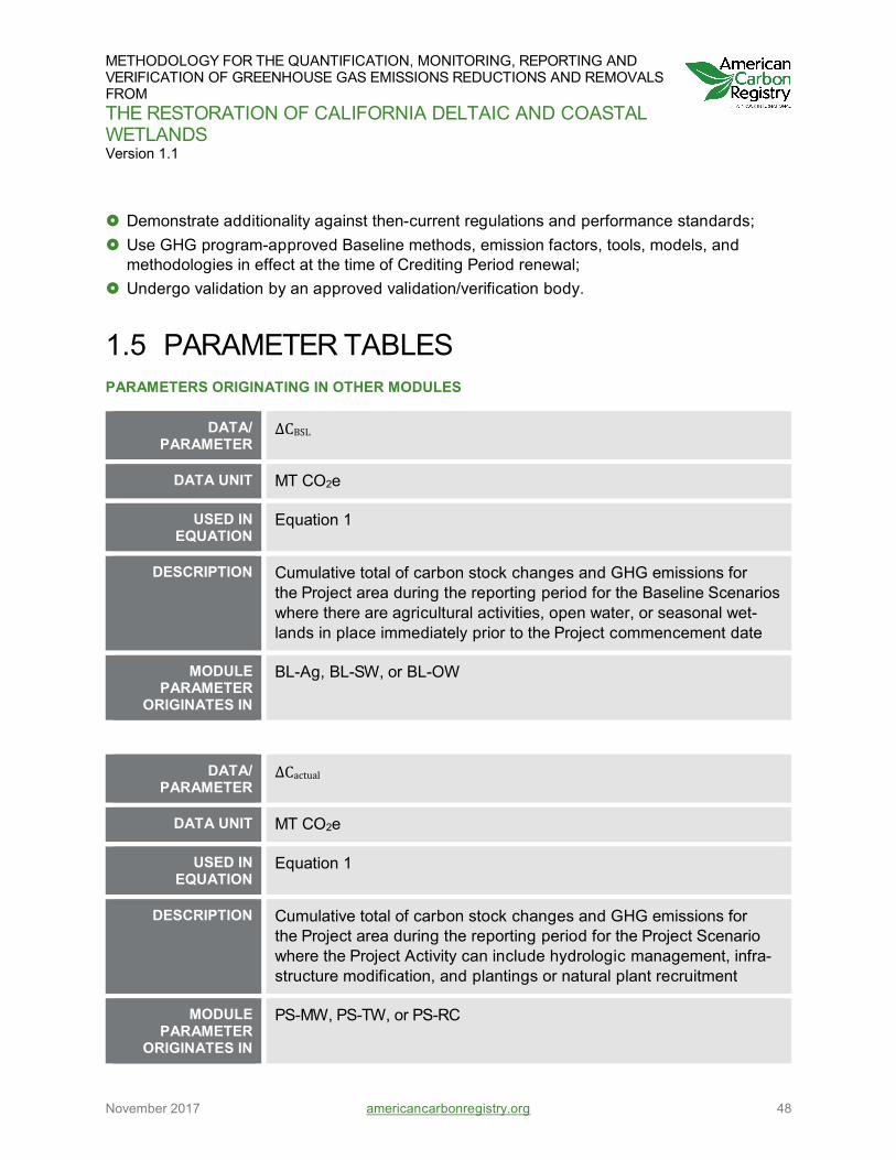
METHODOLOGY FOR THE QUANTIFICATION, MONITORING, REPORTING AND VERIFICATION OF GREENHOUSE GAS EMISSIONS REDUCTIONS AND REMOVALS FROM THE RESTORATION OF CALIFORNIA DELTAIC AND COASTAL WETLANDS Version 1.1
November 2017 americancarbonregistry.org 48
Demonstrate additionality against then-current regulations and performance standards; Use GHG program-approved Baseline methods, emission factors, tools, models, and
methodologies in effect at the time of Crediting Period renewal; Undergo validation by an approved validation/verification body.
1.5 PARAMETER TABLES PARAMETERS ORIGINATING IN OTHER MODULES
DATA/ PARAMETER
ΔCBSL
DATA UNIT MT CO2e
USED IN EQUATION
Equation 1
DESCRIPTION Cumulative total of carbon stock changes and GHG emissions for the Project area during the reporting period for the Baseline Scenarios where there are agricultural activities, open water, or seasonal wet-lands in place immediately prior to the Project commencement date
MODULE PARAMETER
ORIGINATES IN
BL-Ag, BL-SW, or BL-OW
DATA/ PARAMETER
ΔCactual
DATA UNIT MT CO2e
USED IN EQUATION
Equation 1
DESCRIPTION Cumulative total of carbon stock changes and GHG emissions for the Project area during the reporting period for the Project Scenario where the Project Activity can include hydrologic management, infra-structure modification, and plantings or natural plant recruitment
MODULE PARAMETER
ORIGINATES IN
PS-MW, PS-TW, or PS-RC
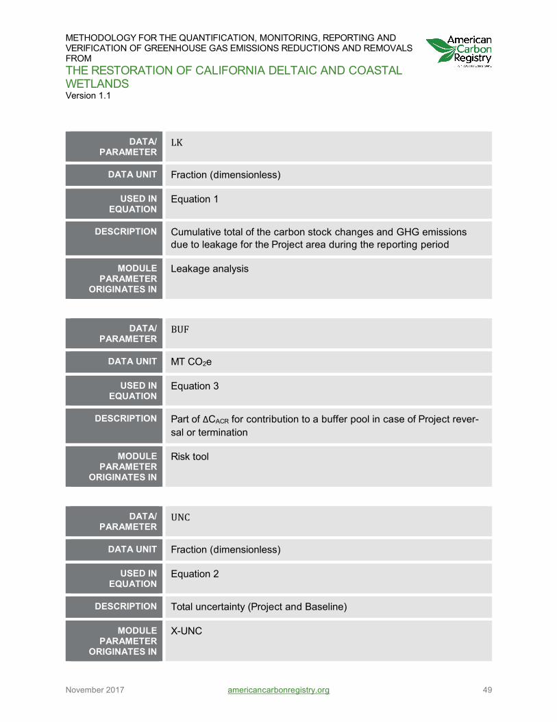
METHODOLOGY FOR THE QUANTIFICATION, MONITORING, REPORTING AND VERIFICATION OF GREENHOUSE GAS EMISSIONS REDUCTIONS AND REMOVALS FROM THE RESTORATION OF CALIFORNIA DELTAIC AND COASTAL WETLANDS Version 1.1
November 2017 americancarbonregistry.org 49
DATA/ PARAMETER
LK
DATA UNIT Fraction (dimensionless)
USED IN EQUATION
Equation 1
DESCRIPTION Cumulative total of the carbon stock changes and GHG emissions due to leakage for the Project area during the reporting period
MODULE PARAMETER
ORIGINATES IN
Leakage analysis
DATA/ PARAMETER
BUF
DATA UNIT MT CO2e
USED IN EQUATION
Equation 3
DESCRIPTION Part of ΔCACR for contribution to a buffer pool in case of Project rever-sal or termination
MODULE PARAMETER
ORIGINATES IN
Risk tool
DATA/ PARAMETER
UNC
DATA UNIT Fraction (dimensionless)
USED IN EQUATION
Equation 2
DESCRIPTION Total uncertainty (Project and Baseline)
MODULE PARAMETER
ORIGINATES IN
X-UNC
METHODOLOGY FOR THE QUANTIFICATION, MONITORING, REPORTING AND VERIFICATION OF GREENHOUSE GAS EMISSIONS REDUCTIONS AND REMOVALS FROM THE RESTORATION OF CALIFORNIA DELTAIC AND COASTAL WETLANDS Version 1.1
November 2017 americancarbonregistry.org 50
2 BASELINE QUANTIFICATION MODULES
PREFACE The objective of this methodology is to describe quantification procedures for the reduction of greenhouse gas (GHG) emissions through conversion of land to wetlands and rice cultivation. This methodology achieves GHG emissions reductions by 1) halting or greatly reducing soil organic carbon oxidation; and 2) increasing soil organic storage by restoring wetlands (tidal and non-tidal) and cultivating rice.
The methodology has been written in a modular format; Project Proponents can choose the ap-plicable Modules for their specific Project and site. First, the Framework Module provides background and an overarching description of the Methodology requirements and Mod-ules. All Projects must meet the requirements outlined in the Methodology Framework Module (MF-W/RC). Next, the remaining Modules provide guidance for Baseline and Project Scenario quantification, methods, modeling, calculation of uncertainty, and other quantification tools. From these supporting Modules, Project Proponents will select the relevant components for a Project.
The Baseline Quantification Modules in this chapter describe conditions, processes and quan-tification procedures of GHGs related to three potential baseline scenarios: (2.1) Baseline con-dition is agriculture (BL-Ag); (2.2) Baseline condition is seasonal wetland (BL-SW); and (2.3) Baseline condition is open water (BL-OW).
Project Proponents must identify the most plausible and credible Baseline Scenario describing what would have occurred in absence of the Project activities.

METHODOLOGY FOR THE QUANTIFICATION, MONITORING, REPORTING AND VERIFICATION OF GREENHOUSE GAS EMISSIONS REDUCTIONS AND REMOVALS FROM THE RESTORATION OF CALIFORNIA DELTAIC AND COASTAL WETLANDS Version 1.1
November 2017 americancarbonregistry.org 51
2.1 (BL-AG) BASELINE CONDITION IS AGRICULTURE
2.1.1 Scope, Background, Applicability and Parameters
2.1.1.1 SCOPE AND BACKGROUND
This Module provides guidance for estimating carbon stock changes and GHG emissions for agricultural lands in the Sacramento-San Joaquin Delta and coastal California in the Baseline case where the Project activity will be managed wetland construction, tidal wetlands, or rice cultivation. The Module provides specific guidance for identifying the Baseline Scenario, defin-ing the Project GHG boundary, stratification, and estimating carbon stock changes and GHG emissions.
2.1.1.2 APPLICABILITY
The Module is applicable for estimating carbon stock changes and GHG emissions for Base-line Project areas planned for managed wetland construction and/or rice cultivation. Project ac-tivities will occur due to some combination of hydrologic management changes and infrastruc-tural modification with assisted natural regeneration or seeding. Infrastructural modification in-cludes drainage modification and earth moving. Project activities shall meet the applicability conditions in the methodology framework listed under wetland construction and rice cultiva-tion. The following conditions must be met to apply this Module:
The Project area must be on agricultural lands where crops are grown and/or animals are grazed;
Typical crops include but are not limited to field crops such as corn or alfalfa and vegetable crops such as tomatoes, where a drained root zone is required;
Pasture can also be included as Baseline Scenario and animal GHG emissions may be included as Baseline GHG emissions, if a leakage analysis determines animal GHG emissions will not be moved outside the Project boundaries because of the Project;
The Project area must have been used as agricultural land at least 6 out of the 10 years prior to the Project start date.
2.1.1.3 PARAMETERS
This Module provides procedures to determine the following parameter:
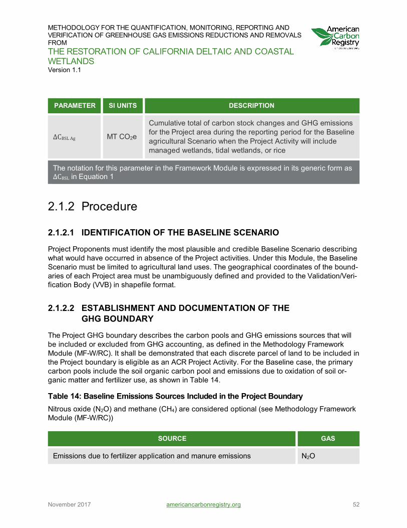
METHODOLOGY FOR THE QUANTIFICATION, MONITORING, REPORTING AND VERIFICATION OF GREENHOUSE GAS EMISSIONS REDUCTIONS AND REMOVALS FROM THE RESTORATION OF CALIFORNIA DELTAIC AND COASTAL WETLANDS Version 1.1
November 2017 americancarbonregistry.org 52
PARAMETER SI UNITS DESCRIPTION
ΔCBSL Ag MT CO2e
Cumulative total of carbon stock changes and GHG emissions for the Project area during the reporting period for the Baseline agricultural Scenario when the Project Activity will include managed wetlands, tidal wetlands, or rice
The notation for this parameter in the Framework Module is expressed in its generic form as ΔCBSL in Equation 1
2.1.2 Procedure
2.1.2.1 IDENTIFICATION OF THE BASELINE SCENARIO
Project Proponents must identify the most plausible and credible Baseline Scenario describing what would have occurred in absence of the Project activities. Under this Module, the Baseline Scenario must be limited to agricultural land uses. The geographical coordinates of the bound-aries of each Project area must be unambiguously defined and provided to the Validation/Veri-fication Body (VVB) in shapefile format.
2.1.2.2 ESTABLISHMENT AND DOCUMENTATION OF THE GHG BOUNDARY
The Project GHG boundary describes the carbon pools and GHG emissions sources that will be included or excluded from GHG accounting, as defined in the Methodology Framework Module (MF-W/RC). It shall be demonstrated that each discrete parcel of land to be included in the Project boundary is eligible as an ACR Project Activity. For the Baseline case, the primary carbon pools include the soil organic carbon pool and emissions due to oxidation of soil or-ganic matter and fertilizer use, as shown in Table 14.
Table 14: Baseline Emissions Sources Included in the Project Boundary Nitrous oxide (N2O) and methane (CH4) are considered optional (see Methodology Framework Module (MF-W/RC))
SOURCE GAS
Emissions due to fertilizer application and manure emissions N2O

METHODOLOGY FOR THE QUANTIFICATION, MONITORING, REPORTING AND VERIFICATION OF GREENHOUSE GAS EMISSIONS REDUCTIONS AND REMOVALS FROM THE RESTORATION OF CALIFORNIA DELTAIC AND COASTAL WETLANDS Version 1.1
November 2017 americancarbonregistry.org 53
SOURCE GAS
Emissions due to oxidation and anaerobic decomposition of soil organic matter and enteric fermentation from livestock
N2O, CO2, CH4
Emissions resulting from fossil fuel combustion CO2
2.1.2.3 BASELINE STRATIFICATION
For estimation of Baseline net GHG removals or emissions, strata shall be defined based on parameters that affect GHG removals or emissions and/or are factors that influence measure-ment of changes in biomass stocks. These may include but are not limited to the factors or practices in Table 15.
Table 15: Factors and Practices that Can Be Used for Stratification and Their Effects on GHG Emissions and Removals
STRATIFICATION FACTOR OR PRACTICE
DESCRIPTION POTENTIAL GHG EFFECT
Vegetation Crop species Affects CO2 sequestration
Soil classification and chemical composition
Soil organic matter, pH, carbon-to-nitro-gen ratio, and texture.
Soil organic matter con-tent is a key determinant of Baseline GHG emis-sions on organic soils. The other factors affect GHG emissions and re-moval.
Hydrology Depth of water and topography (drain ditches, difference in elevation)
Depth of water affects vegetation, thus CO2 se-questration, and GHG emissions.
Agricultural land use
Crop type (hay or grain crop, pasture) Affects Baseline GHG emissions and CO2 sequestration

METHODOLOGY FOR THE QUANTIFICATION, MONITORING, REPORTING AND VERIFICATION OF GREENHOUSE GAS EMISSIONS REDUCTIONS AND REMOVALS FROM THE RESTORATION OF CALIFORNIA DELTAIC AND COASTAL WETLANDS Version 1.1
November 2017 americancarbonregistry.org 54
STRATIFICATION FACTOR OR PRACTICE
DESCRIPTION POTENTIAL GHG EFFECT
Agriculture practices
Harvest, fertilization, etc. Affects carbon stored in the ecosystem and GHG emissions
2.1.2.4 QUANTIFY BASELINE CARBON STOCKS AND GHG EMISSIONS
The Baseline Scenario consists of the most likely projected carbon stock changes and GHG emission in the absence of Project implementation for the life of the Project. The Baseline Sce-nario is fixed for the life of the Project. The Baseline net GHG emissions shall be estimated us-ing the methodology described in this section and in the Methods Module (MM-W/RC). The Methods Module MODEL-W/RC lists requirements for using biogeochemical models, and for using data from sites with sufficiently similar agricultural practices, hydrologic conditions, and soils. For ex-ante calculation of Baseline net GHG emissions, the Project Proponents shall pro-vide estimates of the site-specific values for the appropriate parameters used in the calcula-tions and/or model estimates. Project Proponents shall retain a conservative approach in mak-ing these ex-ante estimates.
The cumulative total carbon stock change and GHG emissions for the agricultural Baseline Scenario is:
Equation 4
𝚫𝚫𝚫𝚫𝐁𝐁𝐁𝐁𝐁𝐁_𝐀𝐀𝐀𝐀 = 𝚫𝚫𝚫𝚫𝐀𝐀𝐁𝐁𝐁𝐁𝐁𝐁_𝐀𝐀𝐀𝐀 + 𝐟𝐟𝐟𝐟𝐟𝐟𝐟𝐟𝐁𝐁𝐁𝐁𝐁𝐁_𝐀𝐀𝐀𝐀 + 𝐟𝐟𝐄𝐄𝐁𝐁𝐁𝐁𝐁𝐁𝐁𝐁𝐁𝐁_𝐀𝐀𝐀𝐀
WHERE
ΔCBSL_Ag is the cumulative total of carbon stock changes and GHG emissions for the agricultural Baseline Scenario for the Project area during the reporting period
ΔCsBSL_Ag is the cumulative carbon stock change for the Project area during the report-ing period
fGHGBSL_Ag is the cumulative total biogenic GHG emissions for the Project area during the reporting period
fEFFBSL_Ag is the emissions of fossil fuels for the Project area during the reporting period

METHODOLOGY FOR THE QUANTIFICATION, MONITORING, REPORTING AND VERIFICATION OF GREENHOUSE GAS EMISSIONS REDUCTIONS AND REMOVALS FROM THE RESTORATION OF CALIFORNIA DELTAIC AND COASTAL WETLANDS Version 1.1
November 2017 americancarbonregistry.org 55
Comment The terms will be added in case GHG exchanges are going in the same direction (from biosphere to atmosphere or vice versa) and subtracted when in opposite directions
When the soil carbon pool includes all components of the ecosystem carbon dynamic, the above equation is reduced to the soil carbon pool change and the fossil fuel emissions (see section 1.3.2.3). The decrease in the soil carbon pool is measured using methods described in the Methods Module (MM-W/RC). For calculation of fossil fuel combustion, see the Methods Module (E-FFC). Double counting shall be avoided. For example, if annual fluxes of CO2, CH4, and N2O are measured in the field or estimated using models, no additional annual soil carbon stock changes should be considered.
2.1.3 Parameter Tables PARAMETERS ORIGINATING IN OTHER MODULES
DATA/ PARAMETER
ΔCBSL_Ag
DATA UNIT MT CO2e
USED IN EQUATION
Equation 4
DESCRIPTION Cumulative C stock changes for the Project area during the reporting period for the Baseline Scenario
MODULE PARAMETER
ORIGINATES IN
MM-W/RC or MODEL-W/RC
COMMENT Baseline C stock changes shall be estimated using techniques de-scribed in the Methods Module MM-W/RC or MODEL-W/RC
DATA/ PARAMETER
fGHGBSL_Ag
DATA UNIT MT CO2e
USED IN EQUATION
Equation 4
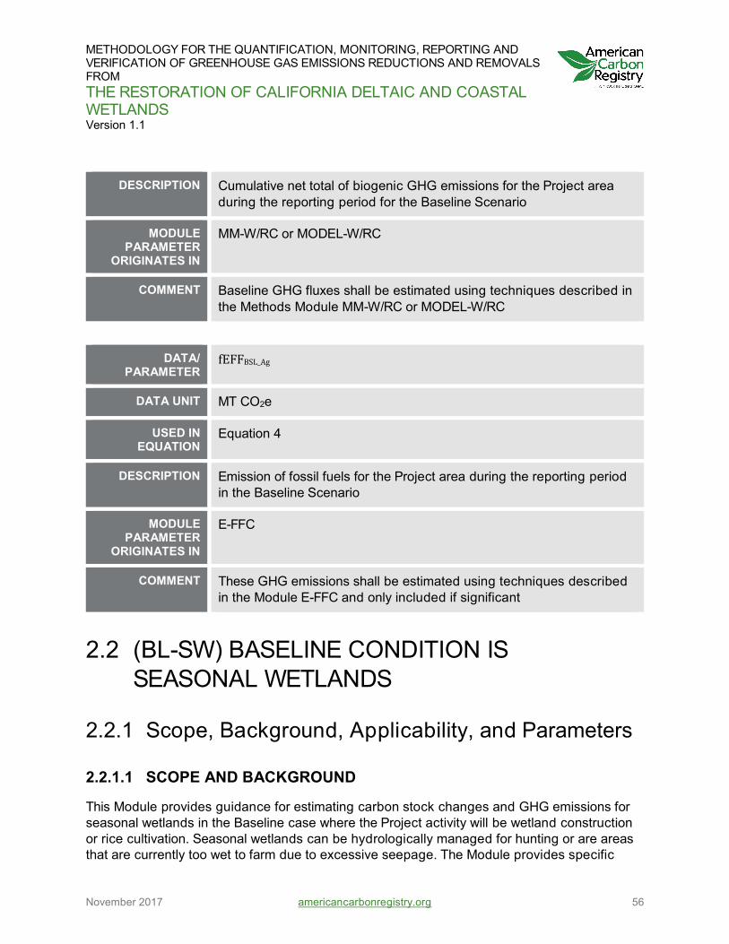
METHODOLOGY FOR THE QUANTIFICATION, MONITORING, REPORTING AND VERIFICATION OF GREENHOUSE GAS EMISSIONS REDUCTIONS AND REMOVALS FROM THE RESTORATION OF CALIFORNIA DELTAIC AND COASTAL WETLANDS Version 1.1
November 2017 americancarbonregistry.org 56
DESCRIPTION Cumulative net total of biogenic GHG emissions for the Project area during the reporting period for the Baseline Scenario
MODULE PARAMETER
ORIGINATES IN
MM-W/RC or MODEL-W/RC
COMMENT Baseline GHG fluxes shall be estimated using techniques described in the Methods Module MM-W/RC or MODEL-W/RC
DATA/ PARAMETER
fEFFBSL_Ag
DATA UNIT MT CO2e
USED IN EQUATION
Equation 4
DESCRIPTION Emission of fossil fuels for the Project area during the reporting period in the Baseline Scenario
MODULE PARAMETER
ORIGINATES IN
E-FFC
COMMENT These GHG emissions shall be estimated using techniques described in the Module E-FFC and only included if significant
2.2 (BL-SW) BASELINE CONDITION IS SEASONAL WETLANDS
2.2.1 Scope, Background, Applicability, and Parameters
2.2.1.1 SCOPE AND BACKGROUND
This Module provides guidance for estimating carbon stock changes and GHG emissions for seasonal wetlands in the Baseline case where the Project activity will be wetland construction or rice cultivation. Seasonal wetlands can be hydrologically managed for hunting or are areas that are currently too wet to farm due to excessive seepage. The Module provides specific

METHODOLOGY FOR THE QUANTIFICATION, MONITORING, REPORTING AND VERIFICATION OF GREENHOUSE GAS EMISSIONS REDUCTIONS AND REMOVALS FROM THE RESTORATION OF CALIFORNIA DELTAIC AND COASTAL WETLANDS Version 1.1
November 2017 americancarbonregistry.org 57
guidance for identifying the Baseline Scenario, defining the Project GHG boundary, stratifica-tion, and estimating carbon stock changes and GHG emissions.
2.2.1.2 APPLICABILITY
The Module is applicable for estimating Baseline GHG emissions and carbon stock changes for Project areas planned for wetland construction or rice cultivation. These land use changes will occur due to some combination of hydrologic management changes and infrastructural modification with assisted natural regeneration or seeding. Infrastructural modification includes drainage modification and earth-moving. The following conditions must be met to apply this Module:
The Project area must be on lands where there are seasonal wetlands; This Module is always mandatory when the Project activity will include wetland construction
and restoration and rice cultivation on lands where there are seasonal wetlands; Seasonal wetlands include areas in the Delta and San Francisco Bay Estuary that may be
used for attracting and breeding waterfowl for hunting, such as duck clubs (Table 16).
Table 16: Examples of Eligible Seasonal Wetlands
SEASONAL WETLAND
TYPE EXAMPLES COMMENTS
Managed seasonal wetlands
Suisun Marsh seasonal wet-lands used for attracting and breeding waterfowl for hunting. There are also seasonal wet-lands used for hunting in the Delta.
Most of the land within Suisun Marsh (85%) consists of diked wetlands that are flooded part of the year and drained from mid-July through mid-September (Chappell 2006; Okamoto and Wong, 2011). These areas have subsided since the 1950s, thus indicating CO2 loss (HydroFocus Inc. 2007).
Unmanaged seasonal wetlands
Many areas of the central Delta where elevations are less than 2 m below sea level have become too wet to farm and are now seasonal wetlands (Deverel et al. 2015).
These areas likely continue to subside and emit carbon dioxide. Miller et al. (2000) and Deverel et al. (1998) demon-strated the net loss of carbon from similar systems in the Delta.

METHODOLOGY FOR THE QUANTIFICATION, MONITORING, REPORTING AND VERIFICATION OF GREENHOUSE GAS EMISSIONS REDUCTIONS AND REMOVALS FROM THE RESTORATION OF CALIFORNIA DELTAIC AND COASTAL WETLANDS Version 1.1
November 2017 americancarbonregistry.org 58
2.2.1.3 PARAMETERS
This Module provides procedures to determine the following parameter:
PARAMETER SI UNIT DESCRIPTION
DCBSL_SW MT CO2e Cumulative total of carbon stock changes and GHG emissions for the Project area during the reporting pe-riod for the seasonal wetlands Baseline Scenario
The notation for this parameter in the Framework Module is expressed in its generic form as ΔCBSL in Equation 1
2.2.2 Procedure
2.2.2.1 IDENTIFICATION OF THE BASELINE ACTIVITIES
Project Proponents must identify the most plausible and credible Baseline Scenario that would have occurred in absence of the Project Activities. Therefore, the Project Proponent needs to demonstrate that seasonal wetlands are the most likely scenario. The geographical coordi-nates of the boundaries of each Project area must be unambiguously defined and provided to the Validation/Verification Body (VVB) in shapefile format.
2.2.2.2 ESTABLISHMENT AND DOCUMENTATION OF THE GHG BOUNDARY
The Project GHG boundary describes the carbon pools that will be included or excluded from GHG accounting. It shall be demonstrated that each discrete parcel of land to be included in the boundary is eligible for wetland or rice Project activity. For the Baseline case, the GHG boundary includes primarily emissions due to oxidation and loss of soil organic carbon. Hydro-logic management and infrastructural modification practices in seasonal wetlands may result in GHG emissions that shall be accounted for. These include emissions associated with earth-moving and vegetation control if determined to be significant. Animal-source GHG emissions can be accounted for the seasonal wetlands Baseline conditions, if leakage analysis shows the animals will not simply move outside the Project area. Exclusion of carbon pools and emission sources is allowed subject to considerations of conservativeness and significance test-ing. Pools or sources can be neglected (i.e., counted as zero) if application of the tool T-SIG indicates that the source is insignificant, i.e., the source represents less than 3% of the ex-ante calculation of GHG emission reductions. If monitoring of Baseline and Project emissions deter-

METHODOLOGY FOR THE QUANTIFICATION, MONITORING, REPORTING AND VERIFICATION OF GREENHOUSE GAS EMISSIONS REDUCTIONS AND REMOVALS FROM THE RESTORATION OF CALIFORNIA DELTAIC AND COASTAL WETLANDS Version 1.1
November 2017 americancarbonregistry.org 59
mines that an emission source(s) initially included in the GHG assessment boundary is insignif-icant using the tool T-SIG, monitoring may cease. The Baseline Scenario consists of the most likely emissions and removals in the absence of Project implementation as shown in Table 17.
Table 17: Baseline Emissions Sources Included in the Project Boundary Nitrous oxide and methane are considered optional (see Methodology Framework Module (MF-W/RC)).
SOURCE GAS
Soil emissions due to fertilizer application N2O
Soil emissions due to oxidation of organic soils N2O, CO2, CH4
Emissions resulting from fossil fuel combustion CO2
2.2.2.3 BASELINE STRATIFICATION
For estimation of Baseline net GHG removals or emissions, or estimation of Project net GHG emission reductions, strata shall be defined based on parameters that affect GHG removals or emissions and/or are factors that influence the measurement of changes in biomass stocks. Potential stratification factors for seasonal wetlands as a Baseline Scenario are listed in Table 18.

METHODOLOGY FOR THE QUANTIFICATION, MONITORING, REPORTING AND VERIFICATION OF GREENHOUSE GAS EMISSIONS REDUCTIONS AND REMOVALS FROM THE RESTORATION OF CALIFORNIA DELTAIC AND COASTAL WETLANDS Version 1.1
November 2017 americancarbonregistry.org 60
Table 18: Factors and Practices that Can Be Used for Stratification and Their Effects on GHG Emissions and Removals
STRATIFICATION FACTOR OR PRACTICE
DESCRIPTION POTENTIAL GHG EFFECT
Wetland management practices
Depth of water Affects vegetation, CO2 sequestration, and CH4 emis-sions
Wetland management practices
Flow through or limited or zero out-flow
Affects CH4 emissions
Wetland vegetation
Variation in species Affects CO2 sequestration
Wetland vegetation
Vegetation establishment (seed-lings, seeds, or natural recruitment)
Affects time required for vegeta-tive cover, CO2 sequestration and CH4 emissions.
Wetland age Years since wetland creation Affects CO2 sequestration
Open water areas
Areas without emergent aquatic vegetation
Minimal CO2 sequestration GHG emissions
Wetland spatial variability
Water circulation Affects CO2 sequestration and GHG emissions
Soil classifica-tion and chemi-cal composition
Soil organic matter, pH, carbon-to-nitrogen ratio, salinity, and texture.
Soil organic matter is a key determinant of Baseline GHG emissions. The other factors affect GHG emissions and removal.
Soil hydrology Depth to groundwater, oxidation- reduction conditions
Depth to groundwater is an im-portant determinant of Baseline GHG emissions on organic soils
For actual Baseline emissions, the stratification for ex-ante estimations shall be based on the Project Monitoring Plan.

METHODOLOGY FOR THE QUANTIFICATION, MONITORING, REPORTING AND VERIFICATION OF GREENHOUSE GAS EMISSIONS REDUCTIONS AND REMOVALS FROM THE RESTORATION OF CALIFORNIA DELTAIC AND COASTAL WETLANDS Version 1.1
November 2017 americancarbonregistry.org 61
2.2.2.4 QUANTIFY BASELINE CARBON STOCKS AND GHG EMISSIONS
The Baseline Scenario consists of the most likely projected emissions and removals in the ab-sence of Project implementation for the life of the Project. The Baseline Scenario is fixed for the life of the Project. The Baseline net GHG emissions shall be estimated using the methodology described in this section and the Measurement Module (MM-W/RC), or using calibrated and validated biogeochemical models as described in the Model Module (MODEL-W/RC). For ex-ante calculation of Baseline net GHG emissions, the Project Proponents shall provide estimates of the site-specific values for the appropriate parameters used in the calculations and/or model estimates. Project Proponents shall retain a conservative approach in making these ex-ante es-timates.
The cumulative total of carbon stock change and GHG emissions for the Baseline seasonal wetlands Scenario is
Equation 5
𝚫𝚫𝚫𝚫𝐁𝐁𝐁𝐁𝐁𝐁_𝐁𝐁𝐒𝐒 = 𝚫𝚫𝚫𝚫𝐀𝐀𝐁𝐁𝐁𝐁𝐁𝐁_𝐁𝐁𝐒𝐒 + 𝐟𝐟𝐟𝐟𝐟𝐟𝐟𝐟𝐁𝐁𝐁𝐁𝐁𝐁_𝐁𝐁𝐒𝐒 + 𝐟𝐟𝐄𝐄𝐁𝐁𝐁𝐁𝐁𝐁𝐁𝐁𝐁𝐁_𝐁𝐁𝐒𝐒
WHERE
ΔCBSL_SW is the cumulative total of carbon stock changes and GHG emissions for the Project area during the reporting period for the seasonal wetlands Baseline Scenario
ΔCsBSL_SW is the cumulative carbon stock change for the Project area during the report-ing period
fGHGBSL_SW is the cumulative net biogenic emissions due to oxidation of organic matter of the Project area during the reporting period
fEFFBSL_SW is the emissions of fossil fuels per Project area during the reporting period
Comment The terms will be added in case GHG exchanges are going in the same direction (from biosphere to atmosphere or vice versa) and subtracted when in opposite directions
Double-counting should be avoided (see section 1.3.2.3).

METHODOLOGY FOR THE QUANTIFICATION, MONITORING, REPORTING AND VERIFICATION OF GREENHOUSE GAS EMISSIONS REDUCTIONS AND REMOVALS FROM THE RESTORATION OF CALIFORNIA DELTAIC AND COASTAL WETLANDS Version 1.1
November 2017 americancarbonregistry.org 62
2.2.3 Parameter Tables PARAMETERS ORIGINATING IN OTHER MODULES
DATA/ PARAMETER
ΔCsBSL_SW
DATA UNIT MT CO2e
USED IN EQUATION
Equation 5
DESCRIPTION Cumulative net carbon stock changes for the Project area during the reporting period for the seasonal wetlands Baseline Scenario
MODULE PARAMETER
ORIGINATES IN
MM-W/RC or MODEL-W/RC
COMMENT Estimated using methods described in Module MM-W/RC or MODEL W/RC
DATA/ PARAMETER
fGHGBSL_SW
DATA UNIT MT CO2e
USED IN EQUATION
Equation 5
DESCRIPTION Cumulative net biogenic emissions due to oxidation of organic matter of the Project area during the reporting period
MODULE PARAMETER
ORIGINATES IN
MM-W/RC or MODEL-W/RC
COMMENT Estimated using methods described in Module MM-W/RC or MODEL-W/RC

METHODOLOGY FOR THE QUANTIFICATION, MONITORING, REPORTING AND VERIFICATION OF GREENHOUSE GAS EMISSIONS REDUCTIONS AND REMOVALS FROM THE RESTORATION OF CALIFORNIA DELTAIC AND COASTAL WETLANDS Version 1.1
November 2017 americancarbonregistry.org 63
DATA/ PARAMETER
fEFFBSL_SW
DATA UNIT MT CO2e
USED IN EQUATION
Equation 5
DESCRIPTION Emission of fossil fuels for the Project area during the reporting period in the Baseline Scenario
MODULE PARAMETER
ORIGINATES IN
E-FFC
COMMENT Estimated using methods described in the Methods Module E-FFC
2.3 (BL-OW) BASELINE CONDITION IS OPEN WATER
2.3.1 Scope, Background, Applicability, and Parameters
2.3.1.1 SCOPE AND BACKGROUND
This Module provides guidance for estimating carbon stock changes and GHG emissions for open water areas in the Baseline case where the Project Activity will be tidal wetland restora-tion. For example, candidate open water areas are primarily former salt ponds located in the San Francisco Bay Estuary. These areas can be potentially converted to tidal wetlands. The Module provides specific guidance for identifying the Baseline Scenario, defining the Project GHG boundary, stratification, and estimating carbon stock changes and GHG emissions.
2.3.1.2 APPLICABILITY
The Module is applicable for estimating Baseline carbon stock changes and GHG emissions for Project areas planned for tidal wetland construction and restoration. This Module is manda-tory when the Project activity includes hydrologic management and infrastructural modification of areas of open water for tidal wetlands including tidal marshes and eelgrass meadows. These land use changes will occur due to some combination of hydrologic management

METHODOLOGY FOR THE QUANTIFICATION, MONITORING, REPORTING AND VERIFICATION OF GREENHOUSE GAS EMISSIONS REDUCTIONS AND REMOVALS FROM THE RESTORATION OF CALIFORNIA DELTAIC AND COASTAL WETLANDS Version 1.1
November 2017 americancarbonregistry.org 64
changes and infrastructural modification with assisted natural regeneration and seeding. Infrastructural modification includes earth-moving, berm and levee construction, drainage modification, and application of dredge materials.
The following condition must be met to apply this Module:
Under this Module, the Baseline Scenario must be limited to open water.
2.3.1.3 PARAMETERS
This Module provides procedures to determine the following parameter:
PARAMETER SI UNIT DESCRIPTION
ΔCBSL_OW MT CO2e Cumulative total of carbon stock changes and GHG emissions for the Project area during the reporting pe-riod for the open water Baseline Scenario
The notation for this parameter in the Methodology Framework Module is expressed in its generic form as ΔCBSL in Equation 1
2.3.2 Procedure
2.3.2.1 IDENTIFICATION OF THE BASELINE ACTIVITIES
Project Proponents must identify the most plausible and credible Baseline Scenario describing what would have occurred in absence of the Project Activities. Under this Module, the Baseline Scenario must be limited to open water. The geographical coordinates of the boundaries of each Project area must be unambiguously defined and provided to the Validation/Verification Body (VVB) in shapefile format.
2.3.2.2 ESTABLISHMENT AND DOCUMENTATION OF THE GHG BOUNDARY
The Project GHG boundary describes the GHG sources and sinks that will be included or ex-cluded from GHG accounting as defined in the Methodology Framework Module (MF-W/RC). It shall be demonstrated that each discrete parcel of land to be included in the boundary is eligi-ble for Project activity. For the open-water Baseline case, emissions will occur due to fossil fuel combustion during dredging operations, infrastructural modification, earth-moving, and con-struction. These emissions must be accounted for if they are determined to be significant. CH4

METHODOLOGY FOR THE QUANTIFICATION, MONITORING, REPORTING AND VERIFICATION OF GREENHOUSE GAS EMISSIONS REDUCTIONS AND REMOVALS FROM THE RESTORATION OF CALIFORNIA DELTAIC AND COASTAL WETLANDS Version 1.1
November 2017 americancarbonregistry.org 65
ebullition may also occur. Emissions shall be estimated based on site/Project-specific data, an acceptable proxy, reference sample plots or field monitoring of similar sites, peer-reviewed lit-erature, approved local parameters, and model estimates. Baseline emissions include GHG emissions within the Project boundary prior to site preparation, or the most likely emissions in the absence of the Project activity (Table 19).
Table 19: Baseline Emissions Sources Included in the Project Boundary
Nitrous oxide and methane are considered optional (see Methodology Framework Module (MF-W/RC)).
SOURCE GAS
Emissions due to oxidation of organic matter CO2, N2O, CH4
Emissions resulting from fossil fuel combustion CO2
Allochthonous carbon may enter the open water area from an outside source and may contrib-ute to carbon accumulation at the site. However, if it represents carbon assimilated by other sinks, the wetland Project area does not contribute to its removal from the atmosphere. For this reason, after it is quantified as described in the Measurement Module (MM-W/RC, Equation 12), it should be deducted from the carbon balance of the Project area. For purposes of this methodology, carbon accumulation from outside sources may be excluded in determination of Baseline GHG emissions or removals if not significant as per guidance in the Methods Module (MM-W/RC and tool T-SIG). Allochthonous carbon accumulation in the Baseline may be con-servatively set to zero, as its exclusion from the balance between GHG losses and gains would underestimate net GHG reductions (i.e., ERTs).
The Project Proponents using emission values from the literature or non-site data must make conservative estimates to determine the Baseline GHG emissions. Exclusion of carbon pools and emission sources is allowed subject to considerations of conservativeness and signifi-cance testing. This may be accomplished by using peer-reviewed literature, reference sample plots or field monitoring of similar sites, approved local or national parameters, the most recent default emission factors provided by the IPCC, government reports, and models. Pools or sources may be excluded if the exclusion tends to underestimate net Project GHG emission reductions (i.e. ERTs). Additional guidance is provided in the Methods Module (MM-W/RC).
Pools or sources can be neglected (i.e., counted as zero) if application of the tool T-SIG (Meth-ods Module section 4.6) indicates that the source is insignificant, i.e., the source represents less than 3% of the ex-ante calculation of GHG emission reductions. If monitoring of Baseline and Project emissions indicate that an emission source(s) initially included in the GHG assess-ment boundary is insignificant using the tool T-SIG, monitoring may cease.

METHODOLOGY FOR THE QUANTIFICATION, MONITORING, REPORTING AND VERIFICATION OF GREENHOUSE GAS EMISSIONS REDUCTIONS AND REMOVALS FROM THE RESTORATION OF CALIFORNIA DELTAIC AND COASTAL WETLANDS Version 1.1
November 2017 americancarbonregistry.org 66
Attention must be used when estimating CH4 emissions in open water in presence of salinity. Salinity can reduce CH4 emissions. Where a default emission factor approach is used based on salinity, the average or low value of salinity shall be measured in shallow pore water or soils within 30 cm of land surface using acceptable technology or analytical determination of total dissolved solids. Sulfate concentrations shall also be determined when salinity is measured us-ing standard analytical methods at a certified laboratory. The salinity average shall be calcu-lated from measurements during periods of peak CH4 emissions. When the frequency of meas-urements is less than monthly for 1 year, the minimum salinity value shall be used. For calcula-tion of CH4 fluxes in presence of salinity, refer to section 3.2.2.4.
2.3.2.3 BASELINE STRATIFICATION
For estimation of Baseline net GHG emissions, strata shall be defined based on parameters that affect GHG emissions. These may include the following:
Depth of open water Water quality (e.g., salinity, nutrient inputs, distance from source, etc.) Soil organic matter content Vegetation Sediment chemical and physical properties (e.g., redox conditions, temperature)
These are the primary factors that affect GHG emissions. If natural or anthropogenic impacts (e.g., levee breaks and flooding) or other factors (e.g., altered hydrology or water manage-ment) add variability in the vegetation of the Project area, then the stratification shall be revised accordingly.
2.3.2.4 QUANTIFY BASELINE CARBON STOCKS AND GHG EMISSIONS
The Baseline Scenario consists of the most likely projected emissions and removals in the ab-sence of Project implementation for the life of the Project. The Baseline Scenario is fixed for the life of the Project. The Baseline net GHG emissions shall be estimated using the methodology described in this section and the Methods Module MM-W/RC or using biogeochemical models responding to requirements listed in the Methods Module MODEL-W/RC. When applying these methods for the calculation of Baseline net GHG removals or emissions, the Project Proponents shall provide estimates of the site-specific values for the appropriate parameters. The Project Proponents shall retain a conservative approach in making these estimates.
Baseline carbon stock changes and GHG emissions for the Baseline reporting period, ΔCBSL_OW
shall be estimated using the following equation for the Baseline reporting period for the Project area.

METHODOLOGY FOR THE QUANTIFICATION, MONITORING, REPORTING AND VERIFICATION OF GREENHOUSE GAS EMISSIONS REDUCTIONS AND REMOVALS FROM THE RESTORATION OF CALIFORNIA DELTAIC AND COASTAL WETLANDS Version 1.1
November 2017 americancarbonregistry.org 67
Equation 6
𝚫𝚫𝚫𝚫𝐁𝐁𝐁𝐁𝐁𝐁_𝐎𝐎𝐒𝐒 = 𝚫𝚫𝚫𝚫𝐀𝐀𝐁𝐁𝐁𝐁𝐁𝐁_𝐎𝐎𝐒𝐒 ∓ 𝐟𝐟𝐟𝐟𝐟𝐟𝐟𝐟𝐁𝐁𝐁𝐁𝐁𝐁_𝐎𝐎𝐒𝐒 + 𝐟𝐟𝐄𝐄𝐁𝐁𝐁𝐁𝐁𝐁𝐁𝐁𝐁𝐁_𝐎𝐎𝐒𝐒
WHERE
ΔCBSL_OW is the cumulative carbon stock change and GHG emissions for the Project area during the reporting period
ΔCsBSL_OW is the cumulative carbon stock change for the Project area during the report-ing period
fGHGBSL_OW is the net emissions of N2O, CO2, and CH4 due to the decomposition of or-ganic matter for the Project area during the reporting period
fEFFBSL_OW is the total emissions as a result of fossil fuel combustion within the Project boundary during the reporting period
Comment The terms will be added in case GHG exchanges are going in the same direction (from biosphere to atmosphere or vice versa) and subtracted when in opposite directions
If deemed significant, the Baseline GHG emissions due to organic matter decomposition from the Project area may be estimated from direct measurement of gaseous fluxes prior to Project activity as described in the Methods Module (MM-W/RC) or determined based on an accepta-ble proxy data, from peer-reviewed literature, or models. Estimation of emissions from fossil fuel combustion shall be estimated as described in the Emissions Module (E-FFC).
2.3.3 Parameter Tables PARAMETERS ORIGINATING IN OTHER MODULES
DATA/ PARAMETER
ΔCsBSL_OW
DATA UNIT MT CO2e
USED IN EQUATION
Equation 6

METHODOLOGY FOR THE QUANTIFICATION, MONITORING, REPORTING AND VERIFICATION OF GREENHOUSE GAS EMISSIONS REDUCTIONS AND REMOVALS FROM THE RESTORATION OF CALIFORNIA DELTAIC AND COASTAL WETLANDS Version 1.1
November 2017 americancarbonregistry.org 68
DESCRIPTION Cumulative net carbon stock changes for the Project area during the reporting period for the open water Baseline Scenario
MODULE PARAMETER
ORIGINATES IN
MM-W/RC or MODEL-W/RC
COMMENT Estimated using measurements (MM-W/RC) or biogeochemical models (Model-W/RC)
DATA/ PARAMETER
fGHGBSL_OW
DATA UNIT MT CO2e
USED IN EQUATION
Equation 6
DESCRIPTION Net GHG emissions (CO2, CH4, N2O) for the Project area during the re-porting period due to the decomposition of organic matter
MODULE PARAMETER
ORIGINATES IN
MM-W/RC or MODEL-W/RC
COMMENT Estimated using measurements (MM-W/RC) or biogeochemical models (MODEL-W/RC)
DATA/ PARAMETER
fEFFBSL_OW
DATA UNIT MT CO2e yr-1
USED IN EQUATION
Equation 6
DESCRIPTION GHG emissions for the Project area over the reporting period as a re-sult of fossil fuel combustion for the Baseline Scenario

METHODOLOGY FOR THE QUANTIFICATION, MONITORING, REPORTING AND VERIFICATION OF GREENHOUSE GAS EMISSIONS REDUCTIONS AND REMOVALS FROM THE RESTORATION OF CALIFORNIA DELTAIC AND COASTAL WETLANDS Version 1.1
November 2017 americancarbonregistry.org 69
MODULE PARAMETER
ORIGINATES IN
E-FFC
COMMENT Estimated using methods described in Module E-FFC

METHODOLOGY FOR THE QUANTIFICATION, MONITORING, REPORTING AND VERIFICATION OF GREENHOUSE GAS EMISSIONS REDUCTIONS AND REMOVALS FROM THE RESTORATION OF CALIFORNIA DELTAIC AND COASTAL WETLANDS Version 1.1
November 2017 americancarbonregistry.org 70
3 PROJECT MODULES
PREFACE The objective of this methodology is to describe quantification procedures for the reduction of greenhouse gas (GHG) emissions through conversion of land to wetlands and rice cultivation. This methodology achieves GHG emissions reductions by 1) halting or greatly reducing soil organic carbon oxidation; and 2) increasing soil organic storage by restoring wetlands (tidal and non-tidal) and cultivating rice.
The methodology has been written in a modular format; Project Proponents can choose the ap-plicable Modules for their specific Project and site. First, the Framework Module provides background and an overarching description of the Methodology requirements and Mod-ules. All Projects must meet the requirements outlined in the Methodology Framework Module (MF-W/RC). Next, the remaining Modules provide guidance for Baseline and Project Scenario quantification, methods, modeling, calculation of uncertainty, and other quantification tools. From these supporting Modules, Project Proponents will select the relevant components for a Project.
The Project Quantification Modules in this chapter describe conditions, processes and quantifi-cation procedures of GHGs related to three potential project scenarios: (3.1) Project condition is managed wetlands (PS-MW); (3.2) Project condition is tidal wetland (PS-TW); and (3.3) Pro-ject condition is rice cultivation (PS-RC).
The methodology is applicable on subsided and/or drained agricultural lands with high organic soil content in California, the majority of which are located in the Sacramento-San Joaquin Delta (“the Delta”) and San Francisco Bay regions.
If, within the Project area, drainage and/or other unplanned and prohibited activities (e.g., flooding) occur, the situation shall be revised. Subsequent documentation shall quantify the ef-fects on GHG emissions, emissions reductions, or GHG sink enhancements.

METHODOLOGY FOR THE QUANTIFICATION, MONITORING, REPORTING AND VERIFICATION OF GREENHOUSE GAS EMISSIONS REDUCTIONS AND REMOVALS FROM THE RESTORATION OF CALIFORNIA DELTAIC AND COASTAL WETLANDS Version 1.1
November 2017 americancarbonregistry.org 71
3.1 (PS-MW) PROJECT CONDITION IS MANAGED WETLANDS
3.1.1 Scope, Background, Applicability, and Parameters
3.1.1.1 SCOPE AND BACKGROUND
This Module provides guidance for estimating ex-ante and ex-post carbon stock changes and GHG emissions related to managed non-tidal wetlands when the Project activity includes hy-drologic management, infrastructural modification, and plantings or natural plant regeneration. Hydrologic management includes alteration of water management practices and water delivery and drainage structures such that drained conditions prevalent for agricultural are eliminated and the land is flooded for wetlands. The Module provides specific guidance for determining applicability, monitoring, Project implementation, stratification, and estimating carbon stock changes and GHG emissions.
3.1.1.2 APPLICABILITY
This Module is always mandatory when the Project Activity includes hydrologic management, infrastructural modification, and plantings or natural plant regeneration for construction of man-aged non-tidal wetlands. Infrastructural modification includes drainage modification and earth-moving. The Baseline Scenario for this Project activity is limited to agriculture and seasonal wetlands.
The following conditions must be met to apply this Module:
The Project area must be on agricultural lands where crops are grown and/or animals are grazed or seasonal wetlands;
Baseline emissions can also include fertilization and enteric livestock fermentation. Animal-source GHG emissions can be included if a leakage assessment shows animals are not transferred outside the Project area;
The Project Activity is implementation of managed non-tidal wetlands.5
5 Managed wetlands can include paludiculture in which the wetland plants are harvested periodically for
economic benefit.

METHODOLOGY FOR THE QUANTIFICATION, MONITORING, REPORTING AND VERIFICATION OF GREENHOUSE GAS EMISSIONS REDUCTIONS AND REMOVALS FROM THE RESTORATION OF CALIFORNIA DELTAIC AND COASTAL WETLANDS Version 1.1
November 2017 americancarbonregistry.org 72
3.1.1.3 PARAMETERS
This Module produces the following parameter.
PARAMETER SI UNIT DESCRIPTION
ΔCactual_MW MT CO2e Cumulative total of carbon stock changes and GHG emissions for the Project area during the reporting pe-riod under the managed wetlands Project
The notation for this parameter in the Methodology Framework Module is expressed in its generic form as ΔCactual in Equation 1
3.1.2 Procedure
3.1.2.1 ESTABLISHMENT AND DOCUMENTATION OF THE GHG BOUNDARY
Information to delineate the Project boundary may include the following:
USGS topographic map or property parcel map where the Project boundary is recorded for all areas of land. Provide the name of the Project area (e.g., compartment number, allotment number);
Local name and a unique ID for each discrete parcel of land; Aerial map (e.g., orthorectified aerial photography or georeferenced remote sensing
images); Geographic coordinates for the Project boundary, total land area, and land holder and user
rights.
A Geographic Information System shapefile that specifies Project boundary locations and re-lated information is required.
3.1.2.1.1 Consideration of Sea Level Rise
If relevant in the determination of geographical Project boundaries and strata, Project Propo-nents shall estimate relative sea level rise and assess its effects over the Crediting period. For both the Baseline and Project Scenarios, the Project Proponent shall estimate relative sea level rise within the Project area based on peer-reviewed literature and/or federal, state, and re-

METHODOLOGY FOR THE QUANTIFICATION, MONITORING, REPORTING AND VERIFICATION OF GREENHOUSE GAS EMISSIONS REDUCTIONS AND REMOVALS FROM THE RESTORATION OF CALIFORNIA DELTAIC AND COASTAL WETLANDS Version 1.1
November 2017 americancarbonregistry.org 73
gional planning documents applicable to the region. The assessment of potential wetland mi-gration, inundation, and erosion with projected sea level rise must account for topographical slope, management, sediment supply, and tidal range. Project Proponents shall be conserva-tive, i.e., use the upper range of estimated sea level rise values for the 40-year Crediting pe-riod.
3.1.2.1.2 Sources and Sinks
Managed non-tidal wetlands sequester CO2 as biomass. CH4 is the primary emission from managed non-tidal wetlands due to decomposition of organic matter. There are also fossil fuel emissions resultant from wetland construction activities. N2O emissions are generally low and even negative in un-enriched managed wetlands. Under permanently flooded soil conditions, N2O is consumed during denitrification and converted to N2 (Butterbach-Bahl et al. 2013).
3.1.2.2 PROJECT STRATIFICATION
In the GHG Project Plan, Project Proponents shall present an ex-ante stratification of the Pro-ject area or justify the absence of stratification. Stratification for ex-ante estimations shall be de-scribed in the Project Management Plan. Table 20 provides typical factors and practices that can be used for stratification.
Strata shall be delineated using spatial data (e.g., maps, GIS, classified imagery). Strata must be spatially discrete and stratum areas must be known. Areas of individual strata must sum to the total Project Area.
Table 20: Factors and Practices that Can Be Used for Stratification and Their Effects on GHG Emissions and Removals
STRATIFICATION FACTOR OR PRACTICE DESCRIPTION POTENTIAL GHG EFFECT
Wetland management practices and infra-structural modification variations
Depth of water and land surface elevation, exca-vated and filled areas
Affects CO2 sequestration and CH4 emissions and vegetation
Infrastructural modifications affect fossil fuel emissions
Wetland management practices
For example, flow through or limited or zero outflow
Affects CH4 emissions
Wetland vegetation Plant species Affects CO2 sequestration

METHODOLOGY FOR THE QUANTIFICATION, MONITORING, REPORTING AND VERIFICATION OF GREENHOUSE GAS EMISSIONS REDUCTIONS AND REMOVALS FROM THE RESTORATION OF CALIFORNIA DELTAIC AND COASTAL WETLANDS Version 1.1
November 2017 americancarbonregistry.org 74
STRATIFICATION FACTOR OR PRACTICE DESCRIPTION POTENTIAL GHG EFFECT
Wetland vegetation Vegetation establishment (seedlings, seed, natural recruitment)
Affects time required for vegetative cover, thus CO2 sequestration and CH4 emissions
Wetland age Years since wetland creation
Affects CO2 sequestration
Open water areas Areas without emergent aquatic vegetation
Minimal CO2 sequestration, GHG emissions
Wetland spatial variability
Water circulation Affects CO2 sequestration and GHG emissions
Soil classification and chemical composition
Soil organic matter, pH, carbon-to-nitrogen ratio, salinity, and texture
Soil organic matter is key determi-nant of Baseline GHG emissions. The other factors affect GHG emis-sions and removal
Soil hydrology Depth to groundwater, oxidation-reduction con-ditions
Depth to groundwater is an im-portant determinant of GHG emis-sions
3.1.2.3 MONITORING PROJECT IMPLEMENTATION
As described in the Methodology Framework Module (MF-W/RC), Project Proponents shall in-clude a single Monitoring Plan in the GHG Project Plan that includes a description of Baseline and Project monitoring and estimation of carbon stock changes and GHG emissions. Information shall be provided, to document that:
The geographic coordinates of the Project boundary (and any stratification inside the boundary) are established, recorded, and archived;
Standard operating procedures (SOPs) and quality control/quality assurance (QA/QC) procedures for field data collection and data management are applied;
Use or adaptation of relevant practices already applied in managed wetland monitoring, or available from published relevant materials, are implemented;
The Monitoring Plan, together with a record of implemented practices and monitoring during the Project duration, shall be available for validation and verification. Information on sampling methodologies and associated uncertainty for managed wetlands can be

METHODOLOGY FOR THE QUANTIFICATION, MONITORING, REPORTING AND VERIFICATION OF GREENHOUSE GAS EMISSIONS REDUCTIONS AND REMOVALS FROM THE RESTORATION OF CALIFORNIA DELTAIC AND COASTAL WETLANDS Version 1.1
November 2017 americancarbonregistry.org 75
obtained from a review of the available literature for managed wetlands in the Sacramento-San Joaquin Delta. For example, Miller et al. (2008) provided data on spatial variability of sedimentation erosion table and coring measurements that can help guide plot and instrumentation placement.
3.1.2.4 QUANTIFY PROJECT CARBON STOCK CHANGES AND GHG EMISSIONS
Carbon stock changes and GHG emissions shall be estimated using the methodology de-scribed in the Methods Module. The methods listed in the Measurement Module (MM-W/RC) may be used alone or in tandem. Carbon stock changes and GHG emissions can be estimated using appropriate peer-reviewed proxy measurement data for similar situations, in which case the environmental setting for the estimates shall be detailed. Also, there shall be an in-depth demonstration of conservativeness and applicability. Biogeochemical models that meet re-quirements listed in the Model Module (MODEL-W/RC) can be used for estimating carbon stock changes and GHG emissions. For example, the peer-reviewed biogeochemical model, Peatland Ecosystem Photosynthesis, Respiration, and Methane Transport model (PEPRMT, see Appendix C), can be used for estimation of CO2 and CH4 exchange from non-tidal, managed wetlands in the Sacramento-San Joaquin Delta.
Parameter estimates shall be based on measured data or published data that can be demon-strated as applicable. If different values for a parameter used in models or calculations are equally plausible, a value that does not lead to over-estimation of net GHG emission reductions must be selected and its use shall be documented. If Project activities include moving sedi-ments, fossil fuel combustion emissions must be quantified during Project activities using methods described in the Method Module E-FFC if determined to be significant, using the tool T-SIG. An ex-ante estimate of fuel consumption shall be made based on projected fuel usage.
Measurement methods to quantify C stocks changes and GHG emissions are described in the Methods Module (MM-W/R). Carbon pools include biomass and soil organic carbon stock changes. Acceptable methods include eddy covariance and soil coring.
A 5-year interval is considered adequate for the determination of changes in soil carbon stocks in managed wetlands. Specifically, soil coring for measurements of soil carbon stock changes can be conducted every 5 years after Project inception and placement of feldspar markers. If eddy covariance measurements are used to estimate carbon stock changes, continual moni-toring shall occur from Project inception unless another method is selected in combination with eddy covariance (such as a biogeochemical model). Project Proponents shall demonstrate that spatial and temporal heterogeneity is adequately represented in the calculation of the emission reductions. Peer-reviewed biogeochemical models calibrated and validated for Project condi-tions can be used to simulate Project carbon stock changes and GHG emissions at 5-year in-tervals. See the Model Module (MODEL-W/RC) for model-use requirements.
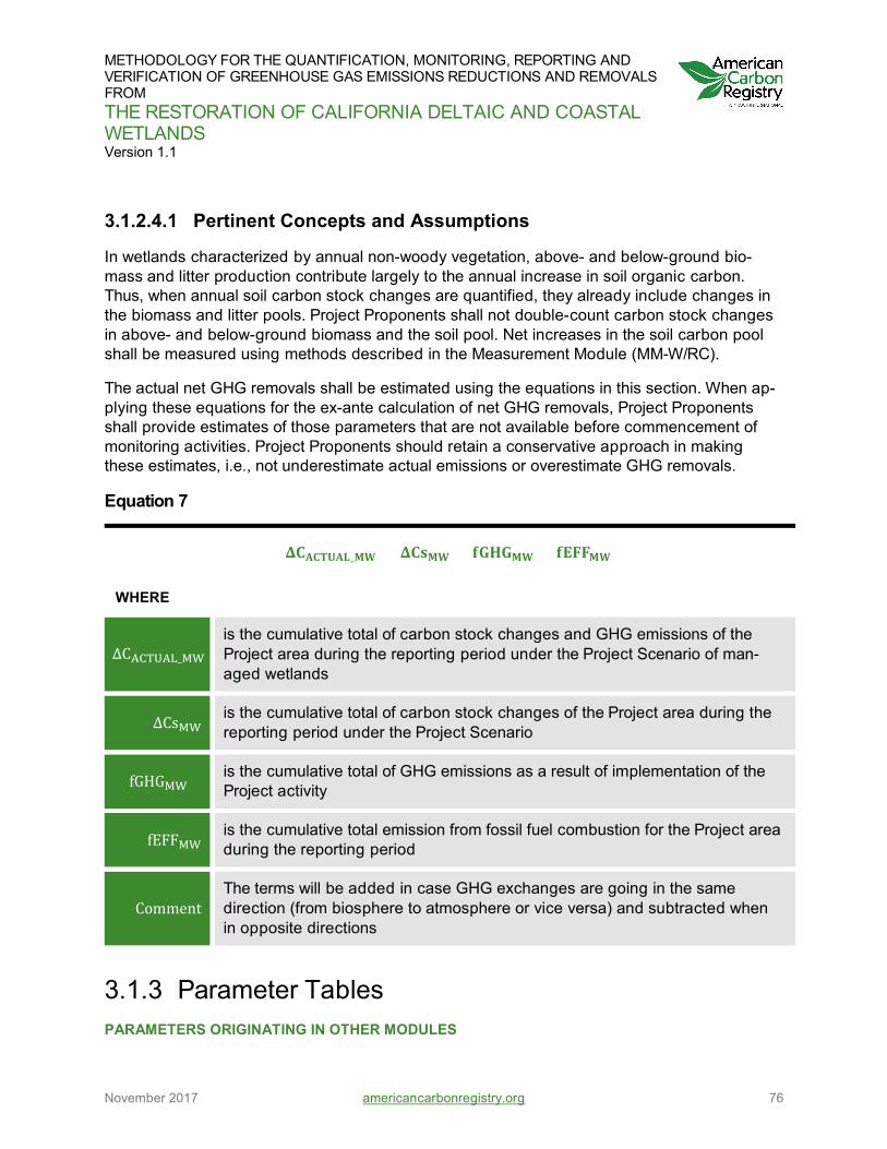
METHODOLOGY FOR THE QUANTIFICATION, MONITORING, REPORTING AND VERIFICATION OF GREENHOUSE GAS EMISSIONS REDUCTIONS AND REMOVALS FROM THE RESTORATION OF CALIFORNIA DELTAIC AND COASTAL WETLANDS Version 1.1
November 2017 americancarbonregistry.org 76
3.1.2.4.1 Pertinent Concepts and Assumptions
In wetlands characterized by annual non-woody vegetation, above- and below-ground bio-mass and litter production contribute largely to the annual increase in soil organic carbon. Thus, when annual soil carbon stock changes are quantified, they already include changes in the biomass and litter pools. Project Proponents shall not double-count carbon stock changes in above- and below-ground biomass and the soil pool. Net increases in the soil carbon pool shall be measured using methods described in the Measurement Module (MM-W/RC).
The actual net GHG removals shall be estimated using the equations in this section. When ap-plying these equations for the ex-ante calculation of net GHG removals, Project Proponents shall provide estimates of those parameters that are not available before commencement of monitoring activities. Project Proponents should retain a conservative approach in making these estimates, i.e., not underestimate actual emissions or overestimate GHG removals.
Equation 7
𝚫𝚫𝚫𝚫𝐀𝐀𝚫𝚫𝐄𝐄𝐔𝐔𝐀𝐀𝐁𝐁_𝐌𝐌𝐒𝐒 = 𝚫𝚫𝚫𝚫𝐀𝐀𝐌𝐌𝐒𝐒 + 𝐟𝐟𝐟𝐟𝐟𝐟𝐟𝐟𝐌𝐌𝐒𝐒 + 𝐟𝐟𝐄𝐄𝐁𝐁𝐁𝐁𝐌𝐌𝐒𝐒
WHERE
ΔCACTUAL_MW is the cumulative total of carbon stock changes and GHG emissions of the Project area during the reporting period under the Project Scenario of man-aged wetlands
ΔCsMW is the cumulative total of carbon stock changes of the Project area during the reporting period under the Project Scenario
fGHGMW is the cumulative total of GHG emissions as a result of implementation of the Project activity
fEFFMW is the cumulative total emission from fossil fuel combustion for the Project area during the reporting period
Comment The terms will be added in case GHG exchanges are going in the same direction (from biosphere to atmosphere or vice versa) and subtracted when in opposite directions
3.1.3 Parameter Tables PARAMETERS ORIGINATING IN OTHER MODULES

METHODOLOGY FOR THE QUANTIFICATION, MONITORING, REPORTING AND VERIFICATION OF GREENHOUSE GAS EMISSIONS REDUCTIONS AND REMOVALS FROM THE RESTORATION OF CALIFORNIA DELTAIC AND COASTAL WETLANDS Version 1.1
November 2017 americancarbonregistry.org 77
DATA/ PARAMETER
ΔCs_MW
DATA UNIT MT CO2e
USED IN EQUATION
Equation 7
DESCRIPTION Cumulative total of carbon stock changes for the Project area during the reporting period under the managed wetland Project Scenario
MODULE PARAMETER
ORIGINATES IN
MM-W/RC or MODEL-W/RC
COMMENT Relevant information shall be included in the GHG Project Plan
DATA/ PARAMETER fGHGMW
DATA UNIT MT CO2e
USED IN EQUATION Equation 7
DESCRIPTION Cumulative total of GHG emissions for the Project area during the re-porting period as a result of implementation of the Project Activity
MODULE PARAMETER
ORIGINATES IN MM-W/RC or MODEL-W/RC
COMMENT Relevant information shall be included in the GHG Project Plan
DATA/ PARAMETER fEFFMW
DATA UNIT MT CO2e

METHODOLOGY FOR THE QUANTIFICATION, MONITORING, REPORTING AND VERIFICATION OF GREENHOUSE GAS EMISSIONS REDUCTIONS AND REMOVALS FROM THE RESTORATION OF CALIFORNIA DELTAIC AND COASTAL WETLANDS Version 1.1
November 2017 americancarbonregistry.org 78
USED IN EQUATION Equation 7
DESCRIPTION Cumulative total emission from fossil fuel combustion for the Project area during the reporting period
MODULE PARAMETER
ORIGINATES IN E-FFC
COMMENT Included if fossil fuel combustion emissions have been determined to be significant using Tool T-SIG
3.2 (PS-TW) PROJECT CONDITION IS TIDAL WETLANDS
3.2.1 Scope, Background, Applicability, and Parameters
3.2.1.1 SCOPE AND BACKGROUND
This Module provides guidance for estimating ex-ante and ex-post carbon stock changes and GHG emissions related to tidal wetlands construction and restoration. The Module provides specific guidance for determining applicability, monitoring Project implementation, stratifica-tion, and estimating carbon stock changes and GHG emissions.
3.2.1.2 APPLICABILITY
This Module is always mandatory for use with tidal wetlands. Tidal wetland restoration includes tidal marshes and eelgrass meadows in the San Francisco Bay Estuary. Hydrologic manage-ment and the infrastructural modification activities requirement for implementation of tidal wet-lands include levee breaching and construction, earth-moving, levee construction, and other activities related to re-introducing tidal action and application of dredged material. The follow-ing conditions must be met to apply this Module:
The Project activity is restoration of tidal wetlands where the Baseline Scenario is seasonal wetlands, agricultural lands, or open water;
This Module is not applicable where application of nitrogen fertilizer(s), such as chemical fertilizer or manure, occurs in the Project area during the Crediting period.

METHODOLOGY FOR THE QUANTIFICATION, MONITORING, REPORTING AND VERIFICATION OF GREENHOUSE GAS EMISSIONS REDUCTIONS AND REMOVALS FROM THE RESTORATION OF CALIFORNIA DELTAIC AND COASTAL WETLANDS Version 1.1
November 2017 americancarbonregistry.org 79
3.2.1.3 PARAMETERS
This Module produces the following parameter.
PARAMETER SI UNIT DESCRIPTION
ΔCactual_TW MT CO2e Cumulative total of carbon stock changes and GHG emissions for the Project area during the reporting pe-riod under the tidal wetland Project Scenario
The notation for this parameter in the Methodology Framework Module is expressed in its generic form as ΔCactual in Equation 1
3.2.2 Procedure
3.2.2.1 ESTABLISHMENT AND DOCUMENTATION OF THE GHG BOUNDARY
Guidance for definition of geographic and temporal boundaries is provided in the Methodology Framework Module (MF-W/RC). The Project Proponent must provide a detailed description of the geographic boundaries for Project activities. Project activities may occur on more than one discrete area of land, and each area must meet the Project eligibility requirements.
3.2.2.1.1 Consideration of Sea Level Rise
In the determination of geographical Project boundaries and strata, Project Proponents shall estimate relative sea level rise and assess the potential for expanding the Project area to ac-count for wetland migration, inundation, and erosion over the Project period. The Project Pro-ponent shall estimate relative sea level rise within the Project area based on peer-reviewed lit-erature and/or federal, state, and regional planning documents applicable to the region. The assessment of potential wetland migration, inundation, and erosion with projected sea level rise must account for topographical slope, management, sediment supply, and tidal range. Project Proponents shall be conservative, i.e., use the upper range of estimated sea level rise values for the 40-year Project period.
When assessing the horizontal migration potential of tidal wetlands, Project Proponents must consider the topography of the adjacent lands and any migration barriers that may exist. In general, concave-up slopes may cause “coastal squeeze,” while straight or convex-up gradi-ents are more likely to provide the space required for lateral movement. The potential for tidal wetlands to rise vertically with sea level rise is sensitive to suspended sediment loads in the system. Project Proponents may use available peer-reviewed data and models to estimate

METHODOLOGY FOR THE QUANTIFICATION, MONITORING, REPORTING AND VERIFICATION OF GREENHOUSE GAS EMISSIONS REDUCTIONS AND REMOVALS FROM THE RESTORATION OF CALIFORNIA DELTAIC AND COASTAL WETLANDS Version 1.1
November 2017 americancarbonregistry.org 80
sediment load thresholds above which wetlands are not predicted to be submerged (Swanson et al. 2015). The vulnerability of tidal wetlands to sea level rise and conversion to open water is also related to tidal range. In general, the most vulnerable tidal wetlands are those in areas with a small tidal range, those with elevations low in the tidal frame, and those in locations with low suspended sediment loads.
3.2.2.2 PROJECT STRATIFICATION
Strata shall be delineated using spatial data (e.g., maps, GIS, classified imagery). Strata must be spatially discrete and stratum areas must be known. Areas of individual strata must sum to the total Project area. For estimation of ex-ante carbon stock changes and GHG emissions, strata should be defined based on parameters that affect carbon sequestration or GHG emis-sions and/or that are key variables for the methods used to measure changes in carbon stocks. Different soil and plant communities will likely have different carbon and GHG dynam-ics. Potential strata criteria are as follows:
Tidal wetland elevation; Vegetation type and species, such as eelgrass meadows; Age class; Water quality (e.g., salinity, nutrient inputs, distance from source, etc.). See discussion
below for relevance to CH4 emissions; Hydrology (e.g., wetland water depth, depth of eelgrass meadow); Soil type (e.g., organic or mineral soils, soil texture); Areas of varying infrastructural modification (e.g., earth-moving).
Tidal wetlands may also be stratified according to salinity with relevance for CH4 emissions. It is generally understood that wetlands exposed to high concentrations of sulfate (an anion pre-sent in seawater) emit CH4 at relatively low rates due to low rates of CH4 production. The pres-ence of sulfate in tidal marsh soils allows sulfate-reducing bacteria to outcompete methano-gens for energy sources, consequently inhibiting CH4 production (Poffenbarger et al. 2011). However, sulfate can be reduced to sulfide in marsh soils or sulfate availability can be limited by diffusion or oxidation-reduction conditions; thus, the inhibitory effect of marine-de-rived saline water can be affected by site-specific conditions that allow CH4 production to per-sist (Megonigal et al. 2004; Weston et al. 2011). Moreover, temporal and spatial variation in sources and sinks for sulfate and CH4 can create conditions where both processes can coexist (Callaway et al. 2012). Therefore, estimates of CH4 emissions and corresponding stratification may require direct measurements or conservative estimates as described below.
Established strata may be merged if reasons for their establishment have disappeared or have proven irrelevant to key variables for estimating net GHG emission reductions. In the GHG Pro-ject Plan, Project Proponents shall present an ex-ante stratification of the Project area or justify

METHODOLOGY FOR THE QUANTIFICATION, MONITORING, REPORTING AND VERIFICATION OF GREENHOUSE GAS EMISSIONS REDUCTIONS AND REMOVALS FROM THE RESTORATION OF CALIFORNIA DELTAIC AND COASTAL WETLANDS Version 1.1
November 2017 americancarbonregistry.org 81
the absence of stratification. Stratification for ex-ante estimations shall be based on the Project Management Plan. Aerial or satellite imagery used to delineate strata shall be verified in the field. The ex-ante defined number and boundaries of the strata may change during the credit-ing period (ex-post). The ex-post stratification shall be updated if natural or anthropogenic im-pacts or other factors add variability to the carbon stock changes or GHG emissions of the Pro-ject area.
3.2.2.2.1 Eelgrass Meadows
Seagrasses that include eelgrass (Zostera marinas) are among the planet’s most effective nat-ural ecosystems for sequestering (capturing and storing) carbon. However, there is limited data and quantifying and modeling their GHG removal capacity is critical for successfully man-aging eelgrass ecosystems to maintain their substantial abatement potential (Macreadie et al. 2014). Given the tendency of eelgrasses to respond differently under different light and depth regimes, projects may differentiate between eelgrass meadow sections that occur at different depths given discrete—or relatively abrupt— bathymetric and substrate changes. For eelgrass meadow restoration Projects in areas with existing eelgrass meadows, Project Proponents must quantify the percentage of natural meadow expansion that can be attributed to the resto-ration effort. Existing meadows are not eligible for inclusion in calculations of Project emissions, even in cases where the restored meadow influences carbon emission rates in existing mead-ows.
New beds that result from natural expansion must be contiguous with restored meadow plots to be included in Project accounting, unless Project Proponents can demonstrate that non-con-tiguous meadow patches originated from restored meadow seeds. This may be done through genetic testing or estimated as a percentage of new meadow in non-contiguous plots ob-served no less than 4 years after the Project start date (McGlathery et al. 2012). This percent-age must not exceed the proportion of restored meadow area relative to the total eelgrass meadow area extent, and Project Proponents must demonstrate the feasibility of current-borne seed dispersal from the restored meadow. In cases where a restored meadow coalesces with an existing meadow(s), Project Proponents must delineate the line at which the two meadows joined. Project Proponents may use either aerial observations showing meadow extent or direct field observations.
3.2.2.3 MONITORING PROJECT IMPLEMENTATION
As described in the Methodology Framework Module (MF-W/RC), Project Proponents shall in-clude a single Monitoring Plan in the Project Plan that includes a description of Baseline and Project monitoring and estimation of carbon stock changes and emissions. Information shall be provided to document the following:
The geographic coordinates of the Project boundary (and any stratification inside the boundary) are established, recorded, and archived;

METHODOLOGY FOR THE QUANTIFICATION, MONITORING, REPORTING AND VERIFICATION OF GREENHOUSE GAS EMISSIONS REDUCTIONS AND REMOVALS FROM THE RESTORATION OF CALIFORNIA DELTAIC AND COASTAL WETLANDS Version 1.1
November 2017 americancarbonregistry.org 82
Standard operating procedures (SOPs) and quality control/quality assurance (QA/QC) procedures for field data collection and data management are applied;
Use or adaptation of relevant practices already applied in tidal wetland monitoring, or available from published relevant materials, are implemented;
The monitoring plan, together with a record of implemented practices and monitoring during the Project, shall be available for validation and verification.
3.2.2.4 QUANTIFY PROJECT CARBON STOCK CHANGES AND GHG EMISSIONS
Carbon stock changes and GHG emissions shall be estimated using the methodology de-scribed in the Methods Module (MM-W/RC), which provides the appropriate methods for measuring and estimating emissions for Project and Baseline activities (use Baseline Modules BL-Ag, BL-OW, or BL-SW). The methods listed in the Methods Module may be used alone or in tandem. For GHG emissions measurements for tidal wetland Project activities, chamber and eddy covariance methods are appropriate. The Methods Module provides guidance, quality assurance and control, precautions and recommendations for chamber and eddy covariance techniques. Emissions can be estimated using appropriate proxy measurements from systems with similar carbon dynamics or estimates for similar situations documented in the peer-re-viewed literature. In this case, the environmental setting for the estimates shall be de-tailed. Also, there shall be a comprehensive demonstration of conservativeness and applicabil-ity.
As discussed above, CH4 fluxes are generally influenced by salinity that can affect stratifica-tion. CH4 emissions can be measured using methods described in the Methods Module. These methods can be used to directly determine and characterize the spatial and temporal variabil-ity resultant from topography, temperature, vegetation, and water levels. Alternatively, a con-servative estimate of CH4 emissions requires measurement in the stratum where and when emissions are likely to be the largest.
That is, chamber or eddy covariance measurements shall be conducted at times and places in which CH4 emissions are expected to be the highest based on expert judgment, datasets, or literature. These are likely to be the wettest strata that support emergent vegetation, but may include stagnant pools of water. If eddy flux towers are used for the conservative approach, they will be placed so that the footprint lies in the stratum with the highest CH4 emissions for at least 50% of the time.
Methodologies used when measuring GHG fluxes under inundated conditions (notably for eel-grass) need to sample and quantify GHG fluxes in different tidal conditions, to prevent under-estimation of GHG emission due to measurements made only during low tides.
Where a default factor approach is used based on salinity, the average or low value of salinity shall be measured in shallow pore water of soils within 30 cm of land surface using acceptable

METHODOLOGY FOR THE QUANTIFICATION, MONITORING, REPORTING AND VERIFICATION OF GREENHOUSE GAS EMISSIONS REDUCTIONS AND REMOVALS FROM THE RESTORATION OF CALIFORNIA DELTAIC AND COASTAL WETLANDS Version 1.1
November 2017 americancarbonregistry.org 83
technology or analytical determination of total dissolved solids. Sulfate concentrations shall also be determined when salinity is measured using standard analytical methods at a certified laboratory. The salinity average shall be calculated from measurements during periods when peak CH4 emissions are expected. When the frequency of salinity measurements is less than monthly for 1 year, the minimum salinity value shall be used.
A default emission factor (Poffenbarger et al. 2011) may be used with caution (see exceptions below) where the salinity average or salinity minimum is greater than 18 parts per thousand. In this case, the annual rate of CH4 emissions (MT CO2e) of a stratum in presence of salinity is:
Equation 8
𝐟𝐟𝐟𝐟𝐟𝐟𝐟𝐟𝐄𝐄𝐒𝐒𝐓𝐓 = 𝟎𝟎.𝟎𝟎𝟎𝟎𝟎𝟎𝟎𝟎 𝐚𝐚 𝚫𝚫𝐟𝐟𝟎𝟎 𝐚𝐚𝐚𝐚𝐚𝐚𝐀𝐀−𝟏𝟏 𝐲𝐲𝐚𝐚−𝟏𝟏 = 𝟎𝟎.𝟎𝟎𝟏𝟏𝟏𝟏 𝐚𝐚 𝚫𝚫𝐟𝐟𝟎𝟎 𝐡𝐡𝐚𝐚−𝟏𝟏 𝐲𝐲𝐚𝐚−𝟏𝟏
The default emission factor shall not be used where oxidation-reduction conditions or sulfate concentrations are such that CH4 production may not be inhibited. For example, Winfrey and Ward (1983) demonstrated greatly increased CH4 pore-water concentrations with decreasing sulfate to chloride ratios in intertidal sediments below 0.01. Morris and Riley (1966) reported a sulfate chloride ratio of 0.14 +/- 0.00023 for the world’s oceans.
Specific applicability conditions follow for the use of the default factor:
The default factor shall not be used when sulfate/chloride ratios are less 0.01; In intertidal areas where sulfate-to-chloride ratios are likely near or below 0.01, CH4 fluxes
shall be measured using methods described in the Methods Module (MM-W/RC).
Project Proponents may also estimate GHG emissions using locally calibrated and peer-re-viewed biogeochemical models as per guidance in the Modeling Module (MODEL-W/RC). Pro-ject Proponents shall provide parameters or data used for modeling during the crediting pe-riod. Parameter estimates shall be based on measured data or existing published data that can be demonstrated as applicable. In addition, Project Proponents must be conservative in estimating parameters. If different values for a parameter used in models or calculations are equally plausible, a value that does not lead to over-estimation of net GHG emission reductions must be selected and its use shall be documented. N2O emissions are generally low, and even negative, in unenriched fresh and coastal marshes (Moseman-Valtierra 2011, 2012; Badiou et al. 2011; Wang et al. 2017; Yu et al. 2007; Liikanen et al 2009).
If Project activities include moving sediments, fossil fuel combustion emissions must be quanti-fied during Project activities using methods described in the Methods Module E-FFC if deter-mined to be significant, using the tool T-SIG. An ex-ante estimate of projected fuel usage shall be made.

METHODOLOGY FOR THE QUANTIFICATION, MONITORING, REPORTING AND VERIFICATION OF GREENHOUSE GAS EMISSIONS REDUCTIONS AND REMOVALS FROM THE RESTORATION OF CALIFORNIA DELTAIC AND COASTAL WETLANDS Version 1.1
November 2017 americancarbonregistry.org 84
Methods for measure above- and below-ground biomass and soil organic carbon stock changes are described in the Methods Module (MM-W/RC). Guidance for use of the mean value or replicate measurements in time and space in estimating carbon stock changes is in the Uncertainty (X-UNC) and Methodology Framework (MF-W/RC) Modules.
A 5-year interval is considered adequate for the determination of changes in soil carbon stocks. Specifically, soil coring measurements of carbon stock changes shall be conducted every 5 years after Project inception and placement of feldspar markers or sediment pins (Macreadie et al. 2014) where opening of the Project area would wash feldspar markers away due to tidal influence. Sediment pins are pounded into the ground to refusal, and sediment ac-cretion is measured against the pin’s height (US Geological Survey 2012).
If eddy covariance measurements are used to estimate carbon stock changes, continual moni-toring shall occur from Project inception until calibrated and validated biogeochemical models documented in the peer-reviewed literature can effectively predict carbon stock changes. See the Model Module (MODEL-W/RC) for model-use requirements. As per guidance in the Meas-urement Module (MM-W/RC), aqueous carbon fluxes shall be accounted for. Project Propo-nents shall demonstrate that spatial and temporal heterogeneity is adequately represented in the estimation of carbon stock changes and GHG emissions. Biogeochemical models cali-brated and validated for Project conditions shall be used to simulate cumulative Project carbon stock changes and GHG emissions for each reporting period.
3.2.2.4.1 Pertinent Concepts and Assumptions
In wetlands characterized by annual non-woody vegetation, over the reporting period, above- and below-ground biomass and litter production represent a large proportion of the increase in the soil carbon pool. Thus, when annual soil carbon stock changes are quantified, they already include changes in the biomass and litter pools. Project Proponents shall not double-count car-bon stock changes in above- and below-ground biomass and the soil pool. Net increases in the soil carbon pool as the result of biomass contributions shall be estimated using methods described in the Methods Module (MM-W/RC).
Project Proponents using non-Project specific values must demonstrate use of conservative es-timates.
Equations and methods for measuring Project carbon stock changes and GHG emissions are provided in the Methods Module (MM-W/RC). The Project carbon stock change and GHG emissions shall be estimated using the equations in this section. In applying these equations ex-ante, Project Proponents shall provide estimates before the start of the Crediting period and monitoring activities. Project Proponents shall utilize a conservative approach in making these estimates. When in the Project Scenario allochthonous soil organic carbon accumulates as in-dicated by aqueous or particulate organic carbon entering the Project area, the net carbon stock change is estimated as follows:

METHODOLOGY FOR THE QUANTIFICATION, MONITORING, REPORTING AND VERIFICATION OF GREENHOUSE GAS EMISSIONS REDUCTIONS AND REMOVALS FROM THE RESTORATION OF CALIFORNIA DELTAIC AND COASTAL WETLANDS Version 1.1
November 2017 americancarbonregistry.org 85
Equation 9
𝚫𝚫𝚫𝚫𝐀𝐀𝚫𝚫𝐄𝐄𝐔𝐔𝐀𝐀𝐁𝐁_𝐄𝐄𝐒𝐒 = 𝚫𝚫𝚫𝚫𝐀𝐀𝐄𝐄𝐒𝐒 + 𝐟𝐟𝐟𝐟𝐟𝐟𝐟𝐟𝐄𝐄𝐒𝐒 − 𝐄𝐄𝐚𝐚𝐄𝐄 + 𝐟𝐟𝐄𝐄𝐁𝐁𝐁𝐁𝐄𝐄𝐒𝐒
WHERE
ΔCACTUAL_TW is the cumulative total of carbon stock changes and GHG emissions (MT CO2e) for the Project area during the reporting period
ΔCsTW is the cumulative total of carbon stock changes under the Project Scenario (MT CO2e) for the Project area during the reporting period
fGHGTW is the cumulative total of biogenic GHG emissions for the Project area during the reporting period as a result of implementation of the Project activity (t CO2e)
Eaq is the deduction to account for allochthonous soil organic carbon (MT CO2e) entering the wetland. See Methods Module (MM-W/RC) for Eaq measure-ments, and T-Sig for determination of significance of this flux
fEFFTW is the total emissions of fossil fuels for the Project area during the reporting period (MT CO2e)
Comment The terms will be added in case GHG exchanges are going in the same direction (from biosphere to atmosphere or vice versa) and subtracted when in opposite directions
Allochthonous carbon may enter the tidal wetland area from an outside source and may con-tribute to carbon accumulation at the site. However, it represents carbon assimilated by other sinks, and the Wetland Project area does not contribute to its removal from the atmosphere. For this reason, it should be quantified and deducted from the total carbon balance of the Pro-ject area, as a loss term. In the Project Scenario, net accumulation of allochthonous carbon must be subtracted from the net carbon balance of a wetland unless the Project Proponent can document that no other entity may claim its GHG emission reductions or removals (i.e., that no other entity may make an ownership claim to the emission reductions or removals for which credits are sought) and if its storage in the tidal wetland decreases the rate of its decomposi-tion compared to what it would be in the absence of the Project (i.e., the case the tidal wetland was not implemented). In the Baseline Scenario, net accumulation of allochthonous carbon can be accounted for and subtracted from the Baseline total carbon stock change, or can be con-servatively set to zero.

METHODOLOGY FOR THE QUANTIFICATION, MONITORING, REPORTING AND VERIFICATION OF GREENHOUSE GAS EMISSIONS REDUCTIONS AND REMOVALS FROM THE RESTORATION OF CALIFORNIA DELTAIC AND COASTAL WETLANDS Version 1.1
November 2017 americancarbonregistry.org 86
3.2.3 Parameter Tables PARAMETERS ORIGINATING IN OTHER MODULES
DATA/ PARAMETER
ΔCsTW
DATA UNIT MT CO2e
USED IN EQUATION
Equation 9
DESCRIPTION Cumulative total of carbon stock changes under the tidal wetland Pro-ject Scenario for the Project area during the reporting period
MODULE PARAMETER
ORIGINATES IN
MM-W/RC or MODEL-W/RC
COMMENT Relevant information shall be included in the GHG Project Plan
DATA/ PARAMETER
fGHGTW
DATA UNIT MT CO2e
USED IN EQUATION
Equation 9
DESCRIPTION Cumulative total of GHG emissions of the Project area during the re-porting period as a result of implementation of the Project activity
MODULE PARAMETER
ORIGINATES IN
MM-W/RC or MODEL-W/RC
COMMENT Relevant information shall be included in the GHG Project Plan

METHODOLOGY FOR THE QUANTIFICATION, MONITORING, REPORTING AND VERIFICATION OF GREENHOUSE GAS EMISSIONS REDUCTIONS AND REMOVALS FROM THE RESTORATION OF CALIFORNIA DELTAIC AND COASTAL WETLANDS Version 1.1
November 2017 americancarbonregistry.org 87
3.3 (PS-RC) PROJECT CONDITION IS RICE CULTIVATION
3.3.1 Scope, Background, Applicability, and Parameters
3.3.1.1 SCOPE AND BACKGROUND
This Module provides methods for estimating ex-ante and ex-post GHG emissions reductions related to rice cultivation (RC). The Module provides specific guidance for determining ap-plicability, monitoring Project implementation, stratification, and estimating carbon stock changes and GHG emissions.
3.3.1.2 APPLICABILITY
This Module is mandatory when the Project activity includes rice cultivation on organic and highly organic mineral soils in the Sacramento-San Joaquin Delta. The Module is applicable for estimating Project carbon stock changes and GHG emissions for Project areas planned for rice cultivation where agriculture is the Baseline Activity as discussed in the agricultural Baseline Module (BL-Ag). The rice cultivation Project activity includes a combination of hydrologic man-agement changes, rice planting, and infrastructural modification. Infrastructural modification includes drainage modification and earth-moving. Hydrologic management includes modifica-tion of existing water supply and drainage facilities to ensure shallow flooding of the rice fields during the spring and summer.
The following conditions must be met to apply this Module:
The Project area must be on agricultural lands where crops are grown and/or animals are grazed on areas of organic soils as in the Sacramento-San Joaquin Delta, or seasonal wetlands;
The Project Activity is rice cultivation where there are organic soils; Best management practices aimed to minimize CH4 emissions and maximize GHG emission
reduction should be used in rice cultivation.
3.3.1.3 PARAMETERS
This Module produces the following parameters:

METHODOLOGY FOR THE QUANTIFICATION, MONITORING, REPORTING AND VERIFICATION OF GREENHOUSE GAS EMISSIONS REDUCTIONS AND REMOVALS FROM THE RESTORATION OF CALIFORNIA DELTAIC AND COASTAL WETLANDS Version 1.1
November 2017 americancarbonregistry.org 88
PARAMETER SI UNIT DESCRIPTION
ΔCactual_RC MT CO2e Cumulative total carbon stock changes and GHG emis-sions for the Project area during the reporting period un-der the Rice cultivation Project Scenario
The notation for this parameter in the Methodology Framework Module is expressed in its generic form as ΔCactual in Equation 1
3.3.2 Procedure
3.3.2.1 ESTABLISHMENT AND DOCUMENTATION OF THE GHG BOUNDARY
The geographic boundaries of a Rice Project are fixed ex-ante. Guidance for defining geo-graphic and temporal boundaries is provided in the Methodology Framework Module (MF-W/RC). The Project Proponent must provide a detailed description of the geographic bounda-ries for Project activities. Project activities may occur on more than one discrete area of land, and each area must meet the Project eligibility requirements.
3.3.2.2 PROJECT STRATIFICATION
If the Project Activity area is not homogeneous (and where applicable), Project Proponents shall implement stratification to improve the accuracy and precision of carbon stock esti-mates. For estimation of ex-ante carbon stocks, strata should be defined based on parameters that affect GHG removal or emissions and/or that are key variables for the methods used to measure changes in carbon stocks. The key factors affecting GHG emissions are fertilization and soil organic carbon contents. Potential strata criteria are described in Table 21.

METHODOLOGY FOR THE QUANTIFICATION, MONITORING, REPORTING AND VERIFICATION OF GREENHOUSE GAS EMISSIONS REDUCTIONS AND REMOVALS FROM THE RESTORATION OF CALIFORNIA DELTAIC AND COASTAL WETLANDS Version 1.1
November 2017 americancarbonregistry.org 89
Table 21: Factors and Practices that Can Be Used for Stratification and Their Effects on GHG Emissions and Removals
STRATIFICATION FACTOR OR PRACTICE DESCRIPTION POTENTIAL GHG EFFECT
Rice water manage-ment practices
Depth of water Affects CO2 sequestration and CH4 emissions
Rice water manage-ment practices
Flow through or limited or zero outflow
Affects CH4 emissions
Rice cultivar Time for maturity varies among cultivars
Affects length of growing season, which affects CO2 sequestration and GHG emissions
Soil classification and chemical composition
Soil organic matter, pH, carbon-to-nitrogen ratio, salinity, and texture
Soil organic matter is a key determi-nant of GHG emissions. The other factors affect GHG emissions and removal
Soil hydrology Depth to groundwater, oxidation-reduction conditions
Depth to groundwater is an im-portant determinant of GHG emis-sions on organic soils
Fertilization rates and timing
Optimum fertilization rates vary for different soils (Espe et al. 2015)
N2O emissions affected by fertiliza-tion rates and timing (Ye and Hor-wath 2014)
In the GHG Project Plan, the Project Proponents shall present an ex-ante stratification of the Project area or justify the absence of stratification. Stratification for ex-ante estimations shall be based on the Project Management Plan. Aerial photography or satellite imagery used to deline-ate strata shall be verified in the field. The ex-ante defined number and boundaries of the strata may change during the Crediting period (ex-post). The ex-post stratification shall be updated if natural or anthropogenic impacts or other factors add variability to the growth pattern or emis-sions of the Project area.

METHODOLOGY FOR THE QUANTIFICATION, MONITORING, REPORTING AND VERIFICATION OF GREENHOUSE GAS EMISSIONS REDUCTIONS AND REMOVALS FROM THE RESTORATION OF CALIFORNIA DELTAIC AND COASTAL WETLANDS Version 1.1
November 2017 americancarbonregistry.org 90
3.3.2.3 MONITORING PROJECT IMPLEMENTATION
As described in the Methodology Framework, Project Proponents shall include a single Moni-toring Plan in the GHG Project Plan that includes a description of Baseline and Project monitor-ing and estimation of carbon stock changes. Information shall be provided in the Monitoring Plan (as part of the Project Plan), to establish the following:
The geographic coordinates of the Project boundary (and any stratification inside the boundary) are established, recorded, and archived;
Commonly accepted principles of rice cultivation for minimizing GHG emissions in the Delta are implemented as described in the Appendix B;
Standard operating procedures (SOPs) and quality control/quality assurance (QA/QC) procedures for field data collection and data management are implemented.
The Monitoring Plan, together with a record of implemented practices and monitoring during the Project, shall be available for validation and verification.
3.3.2.4 QUANTIFY PROJECT CARBON STOCK CHANGES AND GHG EMISSIONS
Carbon stock changes and GHG emissions shall be measured using the methodology de-scribed in this section and the Measurement Module (MM-W/RC), which provides the appropri-ate methods for measuring carbon stocks and GHG emissions for Project activities. The meth-ods listed in the Measurement Module may be used alone or in tandem with the other methods listed. For emission/removal measurements for Rice Cultivation Project activities, chamber and eddy covariance methods are appropriate. Monitoring shall occur during the entire calendar year. Emissions and removals can be estimated using appropriate proxy measurements in sim-ilar situations. If proxy measurements are used, the environmental setting relevance and scien-tific validity shall be detailed. Also, there shall be a demonstration of conservativeness.
Biogeochemical models that meet the requirements described in the Model Module (MODEL-W/RC) can be used for estimating GHG emissions/removals. Project Proponents shall provide transparent calculations or estimates for the parameters used for calculations or modeling dur-ing the Crediting period. These estimates shall be based on measured data or existing pub-lished data where appropriate. In addition, Project Proponents shall apply the principle of con-servativeness. If different values for a parameter are equally plausible, a value that does not lead to demonstrable over-estimation of net GHG emission reductions must be selected. If Pro-ject activities include moving sediments, construction, and the like, fossil fuel combustion emis-sions must be quantified during Project activities using methods described in the Module E-FFC, if determined to be significant using the T-SIG tool. The ex-ante estimate of fuel consump-tion shall be based on projected fuel usage.

METHODOLOGY FOR THE QUANTIFICATION, MONITORING, REPORTING AND VERIFICATION OF GREENHOUSE GAS EMISSIONS REDUCTIONS AND REMOVALS FROM THE RESTORATION OF CALIFORNIA DELTAIC AND COASTAL WETLANDS Version 1.1
November 2017 americancarbonregistry.org 91
Measurement methods can be found in the Measurement Module (MM-W/RC) for calculating carbon stock changes and GHG emissions. If the eddy covariance technique is used, carbon in harvested biomass must be accounted for as described in the Measurement Module. A 5-year frequency is considered adequate for the determination of changes in soil carbon stocks. Project Proponents shall demonstrate that spatial and temporal heterogeneity is ade-quately represented in the estimate of carbon stock changes and GHG emissions.
3.3.2.4.1 Pertinent Concepts and Assumptions
Net increases in the soil carbon pool as the result of biomass contributions shall be estimated using methods described in the Measurement Module (MM-W/RC). Project Proponents shall not double count carbon stock changes in above- and below-ground biomass and the soil pool;
It is assumed that 100% of the harvested biomass is eventually consumed, resulting in releases of CO2 and CH4, back into the atmosphere.The mass of the carbon in the harvested grain shall be counted in the carbon stock change.
Net increases and/or avoided losses in the soil-organic-carbon pool as the result of rice cultivation shall be included;
Exchanges of GHG shall be measured in the field under Project conditions or may be quantified by an acceptable proxy, reference sample plots, or field monitoring of similar sites, using approved local or national parameters, peer-reviewed biogeochemical models, or peer-reviewed literature;
Project Proponents using non-Project specific values must use conservative estimates and demonstrate applicability.
Calculation of ΔCactual_RC (cumulative total of the carbon stock changes and GHG emissions un-der the Project Scenario Rice Cultivation) shall be made using the equations in this section. When applying these equations for the ex-ante calculation of actual net GHG removals by sinks, Project Proponents shall provide estimates of the values of those parameters that are not available before the commencement of monitoring activities. Project Proponents should retain a conservative approach in making these estimates.
The net carbon stock change and GHG emissions are estimated using the following general equation.
Equation 10
𝚫𝚫𝚫𝚫𝐀𝐀𝚫𝚫𝐄𝐄𝐔𝐔𝐀𝐀𝐁𝐁_𝐀𝐀𝚫𝚫 = 𝚫𝚫𝚫𝚫𝐀𝐀𝐀𝐀𝚫𝚫 + 𝐟𝐟𝐟𝐟𝐟𝐟𝐟𝐟𝐀𝐀𝚫𝚫 + 𝐟𝐟𝐄𝐄𝐁𝐁𝐁𝐁𝐀𝐀𝚫𝚫
WHERE
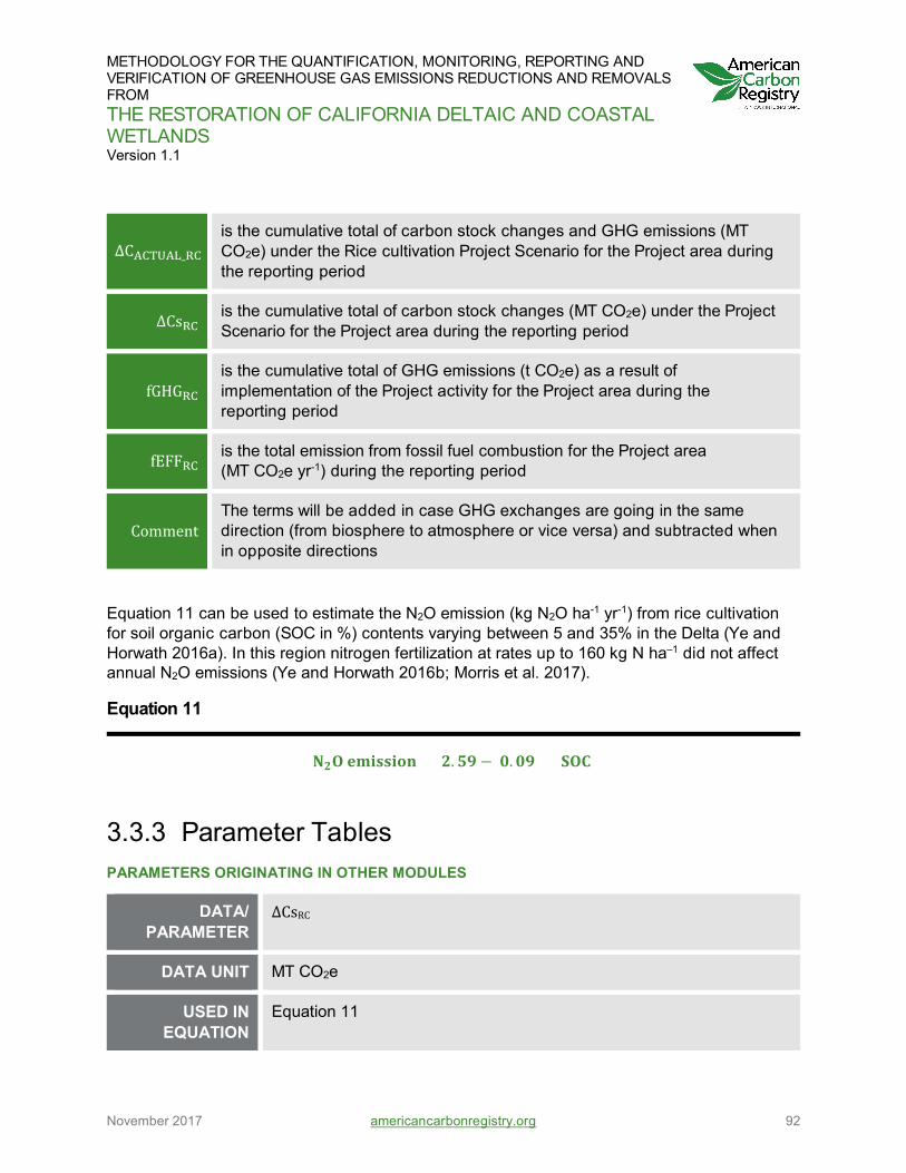
METHODOLOGY FOR THE QUANTIFICATION, MONITORING, REPORTING AND VERIFICATION OF GREENHOUSE GAS EMISSIONS REDUCTIONS AND REMOVALS FROM THE RESTORATION OF CALIFORNIA DELTAIC AND COASTAL WETLANDS Version 1.1
November 2017 americancarbonregistry.org 92
ΔCACTUAL_RC is the cumulative total of carbon stock changes and GHG emissions (MT CO2e) under the Rice cultivation Project Scenario for the Project area during the reporting period
ΔCsRC is the cumulative total of carbon stock changes (MT CO2e) under the Project Scenario for the Project area during the reporting period
fGHGRC is the cumulative total of GHG emissions (t CO2e) as a result of implementation of the Project activity for the Project area during the reporting period
fEFFRC is the total emission from fossil fuel combustion for the Project area (MT CO2e yr-1) during the reporting period
Comment The terms will be added in case GHG exchanges are going in the same direction (from biosphere to atmosphere or vice versa) and subtracted when in opposite directions
Equation 11 can be used to estimate the N2O emission (kg N2O ha-1 yr-1) from rice cultivation for soil organic carbon (SOC in %) contents varying between 5 and 35% in the Delta (Ye and Horwath 2016a). In this region nitrogen fertilization at rates up to 160 kg N ha–1 did not affect annual N2O emissions (Ye and Horwath 2016b; Morris et al. 2017).
Equation 11
𝐔𝐔𝟐𝟐𝐎𝐎 𝐀𝐀𝐞𝐞𝐞𝐞𝐀𝐀𝐀𝐀𝐞𝐞𝐞𝐞𝐞𝐞 = 𝟐𝟐.𝟎𝟎𝟓𝟓 − 𝟎𝟎.𝟎𝟎𝟓𝟓 × 𝐁𝐁𝐎𝐎𝚫𝚫
3.3.3 Parameter Tables PARAMETERS ORIGINATING IN OTHER MODULES
DATA/ PARAMETER
ΔCsRC
DATA UNIT MT CO2e
USED IN EQUATION
Equation 11

METHODOLOGY FOR THE QUANTIFICATION, MONITORING, REPORTING AND VERIFICATION OF GREENHOUSE GAS EMISSIONS REDUCTIONS AND REMOVALS FROM THE RESTORATION OF CALIFORNIA DELTAIC AND COASTAL WETLANDS Version 1.1
November 2017 americancarbonregistry.org 93
DESCRIPTION Cumulative total of carbon stock changes for the Project area during the reporting period under the rice cultivation Project Scenario
MODULE PARAMETER
ORIGINATES IN
MM-W/RC or MODEL-W/RC
COMMENT Relevant information shall be included in the GHG Project Plan
DATA/ PARAMETER
fGHGRC
DATA UNIT MT CO2e
USED IN EQUATION
Equation 11
DESCRIPTION Cumulative total of GHG emissions for the Project area during the re-porting period as a result of implementation of the Project activity
MODULE PARAMETER
ORIGINATES IN
MM-W/R or MODEL-W/RC
COMMENT Relevant information shall be included in the GHG Project Plan
DATA/ PARAMETER
fEFFRC
DATA UNIT MT CO2e
USED IN EQUATION
Equation 11
DESCRIPTION Cumulative total emission from fossil fuel combustion for the Project area during the reporting period

METHODOLOGY FOR THE QUANTIFICATION, MONITORING, REPORTING AND VERIFICATION OF GREENHOUSE GAS EMISSIONS REDUCTIONS AND REMOVALS FROM THE RESTORATION OF CALIFORNIA DELTAIC AND COASTAL WETLANDS Version 1.1
November 2017 americancarbonregistry.org 94
MODULE PARAMETER
ORIGINATES IN
E-FFC
COMMENT Relevant information shall be included in the GHG Project Plan

METHODOLOGY FOR THE QUANTIFICATION, MONITORING, REPORTING AND VERIFICATION OF GREENHOUSE GAS EMISSIONS REDUCTIONS AND REMOVALS FROM THE RESTORATION OF CALIFORNIA DELTAIC AND COASTAL WETLANDS Version 1.1
November 2017 americancarbonregistry.org 95
4 METHODS MODULES
PREFACE The objective of this methodology is to describe quantification procedures for the reduction of greenhouse gas (GHG) emissions through conversion of land to wetlands and rice cultivation. This methodology achieves GHG emissions reductions by 1) halting or greatly reducing soil organic carbon oxidation; and 2) increasing soil organic storage by restoring wetlands (tidal and non-tidal) and cultivating rice.
The methodology has been written in a modular format; Project Proponents can choose the ap-plicable Modules for their specific Project and site. First, the Framework Module provides background and an overarching description of the Methodology requirements and Mod-ules. All Projects must meet the requirements outlined in the Methodology Framework Module (MF-W/RC). Next, the remaining Modules provide guidance for Baseline and Project Scenario quantification, methods, modeling, calculation of uncertainty, and other quantification tools. From these supporting Modules, Project Proponents will select the relevant components for a Project.
The Methods Modules and Tools in this chapter describe: 4.1) how to measure carbon stock changes and GHG emissions (MM-W/RC); 4.2) how to estimate carbon stock changes and GHG emissions using biogeochemical models (MODEL-W/RC); 4.3) how to quantify fossil fuel emissions (E-FFC); 4.4) how to quantify uncertainty (X-UNC); 4.5) how to estimate risks (T-Risk); 4.6) how to conduct significance testing (T-SIG); and 4.7) how to design field plots (T-PLOT).
PARAMETERS Table 22 through Table 24 and Figure 4 below describe the parameters needed to quantify carbon stock changes and GHG emissions for Wetland Restoration and Rice Cultivation Pro-jects. The methodological options for quantifying each variable are listed for each Baseline and Project activity type.
Parameters in Table 24 can be estimated using appropriate measurement data documented in the peer-reviewed literature or estimates from proxy systems. If proxy data are used, documen-tation of sufficiently similar climate, soil, hydrologic conditions, and vegetation conditions are required.

METHODOLOGY FOR THE QUANTIFICATION, MONITORING, REPORTING AND VERIFICATION OF GREENHOUSE GAS EMISSIONS REDUCTIONS AND REMOVALS FROM THE RESTORATION OF CALIFORNIA DELTAIC AND COASTAL WETLANDS Version 1.1
November 2017 americancarbonregistry.org 96
Table 22: Description and Estimation Methods of Carbon Stock Changes and GHG Emissions Parameters for Baseline and Project Scenarios
PARAMETER SI UNIT DESCRIPTION ESTIMATION METHODS
ΔCBSL MT CO2e
Cumulative total of carbon stock changes and GHG emissions for the Baseline Scenario
Biogeochemical models
Eddy covariance
Subsidence measurements
Whole ecosystem chambers
Aqueous carbon flux measurements
C inventories
ΔCactual MT CO2e
Cumulative total of carbon stock changes and GHG emissions for the Project Scenario
Eddy covariance
Biogeochemical models
Soil core collection and analysis using feldspar markers and tidal pins
Aqueous carbon flux measurements
Whole ecosystem chambers
C inventories
Table 23: Emissions Sources Parameters, Description, and Estimation Methods
PARAMETER SI UNIT DESCRIPTION ESTIMATION METHODS
ΔGHGBSL MT CO2e
Cumulative net GHG fluxes for the Baseline Scenario
Chamber measurements
Biogeochemical models
Eddy-covariance measurements
Subsidence measurements
ΔGHGP MT CO2e
Cumulative net GHG fluxes due to Project Activities
Chamber measurements
Biogeochemical models
Eddy covariance
EFFC MT CO2e
Annual GHG emis-sions due to com-bustion of fossil fuel
Module E-FFC, provides guidance for fossil fuel emissions estimates
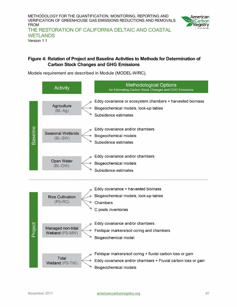
METHODOLOGY FOR THE QUANTIFICATION, MONITORING, REPORTING AND VERIFICATION OF GREENHOUSE GAS EMISSIONS REDUCTIONS AND REMOVALS FROM THE RESTORATION OF CALIFORNIA DELTAIC AND COASTAL WETLANDS Version 1.1
November 2017 americancarbonregistry.org 97
Figure 4: Relation of Project and Baseline Activities to Methods for Determination of Carbon Stock Changes and GHG Emissions
Models requirement are described in Module (MODEL-W/RC).

METHODOLOGY FOR THE QUANTIFICATION, MONITORING, REPORTING AND VERIFICATION OF GREENHOUSE GAS EMISSIONS REDUCTIONS AND REMOVALS FROM THE RESTORATION OF CALIFORNIA DELTAIC AND COASTAL WETLANDS Version 1.1
November 2017 americancarbonregistry.org 98
Table 24: Description and Estimation Methods of Carbon Pools Changes
PARAMETER SI UNIT DESCRIPTION ESTIMATION METHODS
ΔCag biom MT CO2e
Cumulative above-ground carbon stock changes
Allometric equations, leaf area index, digital photography, destructive methods
ΔCbg biom MT CO2e
Cumulative below-ground biomass carbon stock changes
Multiplication of accumulated above-ground biomass times published root:shoot ratio, destructive methods
ΔClitter MT CO2e
Litter carbon stock changes
Direct measurements using decomposi-tion bags or indirect estimates from iso-topic technique and/or modeled esti-mates based on environmental controls
ΔCcr, MT CO2e
Crop residue re-maining in field
Destructive methods for harvest and de-termination of carbon content of biomass
ΔCsoil MT CO2e
Changes in soil carbon stock
Soil coring
4.1 (MM-W/RC) MEASUREMENT METHODS TO ESTIMATE CARBON STOCK CHANGES AND GHG EMISSIONS
4.1.1 Scope This Module provides direction for ex-ante and ex-post estimation of carbon stock changes and GHG emissions for Baseline and Project conditions and data collection for inputs to bioge-ochemical models.

METHODOLOGY FOR THE QUANTIFICATION, MONITORING, REPORTING AND VERIFICATION OF GREENHOUSE GAS EMISSIONS REDUCTIONS AND REMOVALS FROM THE RESTORATION OF CALIFORNIA DELTAIC AND COASTAL WETLANDS Version 1.1
November 2017 americancarbonregistry.org 99
4.1.2 Applicability This Module is applicable for all Baseline conditions and Project activities. The Methodology Framework Module (MF-W/RC) describes the applicable conditions and relevant Project activi-ties for the use of the methodology.
4.1.3 Parameters and Estimation Methods Net exchanges of GHG can be estimated through two different approaches: 1) using a mass balance approach to quantify carbon stock differences between two points in time; or 2) quan-tifying carbon losses and gain. The latter approach focuses on the processes involved and thus on fluxes: biogenic CO2, CH4, and N2O fluxes, and fossil fuel emissions. Some parame-ters, such as soil carbon pools, are more easily and traditionally measured using a mass-bal-ance approach. Others, such as fossil fuel emissions, are only measured as fluxes.
Eddy covariance, chambers, and biogeochemical models measure or estimate carbon uptake and release (or directly measure or estimate their net balance) at any given moment. Their cu-mulative value over time (usually a year) is equivalent to the carbon stock change for that year. Additional C losses or gains from the ecosystem, such as harvested grain and aqueous carbon loads, should be considered in addition to gas exchange measurements. The mass balance approach (Approach 1) can be based on inventories of carbon stocks in the ecosystems and their difference in time. Above-ground biomass, below-ground biomass, dead biomass, litter, soil carbon, and harvested biomass need to be measured at the beginning and end of the re-porting period. The cumulative value of carbon gains and losses over time (usually a year) is equivalent to the carbon stock mass change for that time. Additional methods are possible and can combine mass balance and flux quantification. For example, an additional method to measure the net ecosystem CO2 flux is to measure the difference between NPP (net primary productivity) and the heterotrophic respiration.
The general equations used to quantify biogenic GHG fluxes and C stock changes under both Baseline and Project Scenarios are:
Equation 12
∆𝚫𝚫𝐁𝐁 + 𝐟𝐟𝐟𝐟𝐟𝐟𝐟𝐟 = ����𝐄𝐄𝚫𝚫𝐎𝐎𝟐𝟐,𝐞𝐞 + 𝐄𝐄𝚫𝚫𝐟𝐟𝟎𝟎,𝐞𝐞 + 𝐄𝐄𝐔𝐔𝟐𝟐𝐎𝐎,𝐞𝐞 + 𝚫𝚫𝐀𝐀𝐚𝐚𝐞𝐞 + 𝐄𝐄𝐚𝐚𝐄𝐄�𝐞𝐞
𝐞𝐞=𝟏𝟏
�𝟎𝟎𝟎𝟎
𝐚𝐚=𝟏𝟏
AND
Equation 13

METHODOLOGY FOR THE QUANTIFICATION, MONITORING, REPORTING AND VERIFICATION OF GREENHOUSE GAS EMISSIONS REDUCTIONS AND REMOVALS FROM THE RESTORATION OF CALIFORNIA DELTAIC AND COASTAL WETLANDS Version 1.1
November 2017 americancarbonregistry.org 100
�𝐄𝐄𝚫𝚫𝐎𝐎𝟐𝟐,𝐞𝐞 + 𝐄𝐄𝚫𝚫𝐟𝐟𝟎𝟎,𝐞𝐞� = (∆𝚫𝚫𝐚𝐚𝐀𝐀 𝐛𝐛𝐞𝐞𝐞𝐞𝐞𝐞,𝐞𝐞 + ∆𝚫𝚫𝐛𝐛𝐀𝐀 𝐛𝐛𝐞𝐞𝐞𝐞𝐞𝐞,𝐞𝐞 + ∆𝚫𝚫𝐀𝐀𝐀𝐀𝐚𝐚𝐀𝐀 𝐞𝐞𝐚𝐚𝐚𝐚𝐚𝐚𝐀𝐀𝐚𝐚,𝐞𝐞 + ∆𝚫𝚫𝐀𝐀𝐞𝐞𝐞𝐞𝐚𝐚,𝐞𝐞)
WHERE
ΔCs + fGHG is the cumulative carbon stock changes and/or net emission and removal of CO2, CH4, and N2O (MT CO2e) for the entire Project area during the report-ing period
𝐄𝐄𝚫𝚫𝐎𝐎𝟐𝟐,𝐞𝐞 is the annual net flux of CO2 for the stratum i (MT CO2e yr-1)
𝐄𝐄𝚫𝚫𝐟𝐟𝟎𝟎,𝐞𝐞 is the annual net flux of CH4 for the stratum i (MT CO2e yr-1)
𝐄𝐄𝐔𝐔𝟐𝟐𝐎𝐎,𝐞𝐞 is the annual net flux of N2O for the statum i (MT CO2e.yr-1)
i is the stratum within the Project boundary
n is the number of strata within the Project boundary
Eaqi is the annual net aqueous exchange of carbon in drainage water (MT CO2e yr-1)
t is the year of the Project reporting period
Cgri is the carbon removal in harvested biomass in the stratum (MT CO2e yr-1)
ΔCag_biom,i is above-ground biomass carbon pool change
ΔCbg_biom,i is below-ground biomass carbon pool change
ΔCdead matter,i is the change in litter and dead matter (including crop residues left in the field) carbon pool
ΔCsoil,i is the change in the soil carbon pool
The left part of equation 12 represents annual carbon fluxes measured with eddy covariance or chambers and the right part the sum of the different carbon pools stock changes over the same time. Therefore, over the same period of time, the net GHG removals and emissions cor-respond to the change in carbon stocks of all ecosystem pools.
Signs for the storage and flux terms should be used accordingly. Carbon moving from the at-mosphere to the biosphere will result in a positive storage term (∆CS). However, in case of

METHODOLOGY FOR THE QUANTIFICATION, MONITORING, REPORTING AND VERIFICATION OF GREENHOUSE GAS EMISSIONS REDUCTIONS AND REMOVALS FROM THE RESTORATION OF CALIFORNIA DELTAIC AND COASTAL WETLANDS Version 1.1
November 2017 americancarbonregistry.org 101
GHG fluxes (fGHG and fEFF), a positive sign is often used to indicate emissions to the atmos-phere. The different terms will be added when GHG exchanges are in the same direction (go-ing from biosphere to atmosphere or vice versa), and subtracted when in opposite direction, e.g. when carbon storage counteracts CH4 and N2O emissions.
It is assumed that 100% of the harvested biomass is eventually consumed and released as CO2 and CH4 back into the atmosphere.
Net GHG exchanges should be converted to MT CO2e based on global warming potentials (GWP) in the latest version of ACR Standard.
Each method listed below is discussed with an introduction, method-specific applicability con-ditions, quality control and assurance procedures, and method-specific equations:
Eddy covariance Chamber measurements Harvested grain and biomass Aqueous carbon loads Subsidence measurements Soil coring Biomass carbon pools
Additionally, each method should follow development of international standards as laid out in pertinent scientific literature.
The methods listed can be used in combination with other listed methods. The selection of methods depends on Project and Baseline conditions, data availability, and the requisite level of certainty.
4.1.3.1 EDDY COVARIANCE
This section provides information about the use of eddy covariance techniques to measure gas fluxes.
4.1.3.1.1 Introduction
The eddy covariance (EC) technique (Baldocchi et al. 1988) estimates fluxes of GHGs by rely-ing on the concurrent measurements of fluctuations of vertical wind velocity and atmospheric concentration of GHGs (e.g., CO2, CH4, N2O). Using this method GHG fluxes can be measured at the ecosystem level and on a scale of generally a few hectares. Net ecosystem GHG fluxes

METHODOLOGY FOR THE QUANTIFICATION, MONITORING, REPORTING AND VERIFICATION OF GREENHOUSE GAS EMISSIONS REDUCTIONS AND REMOVALS FROM THE RESTORATION OF CALIFORNIA DELTAIC AND COASTAL WETLANDS Version 1.1
November 2017 americancarbonregistry.org 102
can be monitored for extended periods of time in a continuous manner. This approach is al-lowed for estimating carbon stock changes and GHG emissions for Baseline and Project con-ditions. When EC-measured net carbon flux is cumulated on an annual scale, it is defined as NEE (Net Ecosystem Exchange) or NEP (Net Ecosystem Production).
EC measurements provide an effective way to determine the net exchange of GHGs for a vari-ety of ecosystems and have been used to measure Baseline (Teh et al. 2011) and Project car-bon stock changes (Knox et al. 2015) on organic and highly organic mineral soils in the Delta for more than a decade (see Appendix B for additional information). For agricultural Baseline conditions (e.g., corn) on organic soils, CO2 sequestration occurred as the result of plant pho-tosynthetic uptake during the growing season. Oxidation of organic matter resulted in a net GHG emission. In addition, CO2 assimilated into the harvested grain was removed from the ecosystem and resulted in an overall annual GHG emission. In contrast, for a permanently flooded wetland and, to a lesser extent, rice cultivation, flooding the soil during the warmest time of the year greatly reduced oxidation of soil organic matter resulting in a net GHG removal (Knox et al. 2015). Hatala et al. (2012) quantified GHG fluxes of rice and a pasture on organic soils in the Sacramento-San Joaquin Delta. The rates of carbon removal of rice were slightly lower than those of a riparian cottonwood stand about 50 km east of their site measured by Kochendorfer et al. (2011). The magnitude of CO2 uptake at the Hatala et al. (2012) rice paddy was well below that from a restored marsh in southern California, where net carbon removal measured with EC varied between 6.8 and 18.5 tons CO2 per acre (2.7 and 7.5 tons CO2 ha-1) during an 8-year study (Rocha and Goulden 2008), and higher than historical rates of accumu-lation in disturbed ecosystems of the same region (Canuel et al. 2009).
4.1.3.1.2 Applicability
The following applicability conditions apply to the use of eddy covariance.
Stratification and landscape homogeneity in the EC footprint: The area of land contributing to the measured fluxes (footprint of the EC measurement) shall be quantified during the monitoring period and shall be shown to adequately represent the hydrologic, water quality and soil conditions, and management practices for the stratum. For example, the agricultural crop, water, and land management practices within the EC footprint shall be the same as for the entire stratum. Also, the average soil organic matter content within the EC footprint shall not vary more than 20% relative to the average soil organic matter content within the stratum.
To avoid influences of adjacent land uses, the EC footprint shall be within the stratum that includes Project or Baseline land uses.
The monitoring period using EC techniques shall be sufficient to quantify annual and inter-annual variations in GHG fluxes and to enable the use of biogeochemical models. The Project Proponents shall demonstrate that annual values for carbon stock changes for Baseline are representative. At least 1 year of monitoring is required for Baseline conditions. The Baseline Scenario shall be developed for the entire life of the Project using

METHODOLOGY FOR THE QUANTIFICATION, MONITORING, REPORTING AND VERIFICATION OF GREENHOUSE GAS EMISSIONS REDUCTIONS AND REMOVALS FROM THE RESTORATION OF CALIFORNIA DELTAIC AND COASTAL WETLANDS Version 1.1
November 2017 americancarbonregistry.org 103
site-specific data and/or models responding to requirements described in Module MODEL-W/RC. For Project conditions, continuous monitoring is required throughout the life of the Project unless biogeochemical models are calibrated with the EC data and can adequately predict GHG fluxes as described in Module MODEL-W/RC. At that point, EC measurements can be terminated.
4.1.3.1.3 Quality Assurance and Quality Control
Table 25: Quality Control/Assurance for Eddy Covariance Measurements Describes quality assurance and quality control measures for EC measurements.
QUALITY CONTROL/
ASSURANCE TOPIC
CONSIDERATIONS PROCEDURES
Temporal var-iability and frequency of measure-ments
GHG fluxes shall be measured with the EC method (Baldocchi et al. 1988) using parameters determined to be ade-quate for accurate EC measurements in peat soils and wetlands. Car-bon accumulation rates shall be compared with measurements reported for natural and disturbed ecosystems in the region.
Standard EC practice shall be employed to measure the covariance between turbulence and C fluxes at 10 Hz intervals (every 0.1 s). These data shall be used to calculate half-hourly fluxes for net ecosystem exchange.
Filtering and removal of spurious data
EC data typically contain gaps and artificial spikes.
The sampling rate and averaging interval will allow for a 5 Hz cut-off for the cospectra be-tween turbulence and carbon fluxes. After computing the fluxes, flux values with anom-alously high and low friction velocity (u* > 1.2 m s−1 and |uw| < 0.02) shall be filtered to constrain the analysis to periods where the air near the sensors was well-mixed. The ran-dom instrumental noise in each half-hour fluxes shall be assessed using bootstrapping technique. Fluxes from wind directions out-side of the footprint of the target land-use
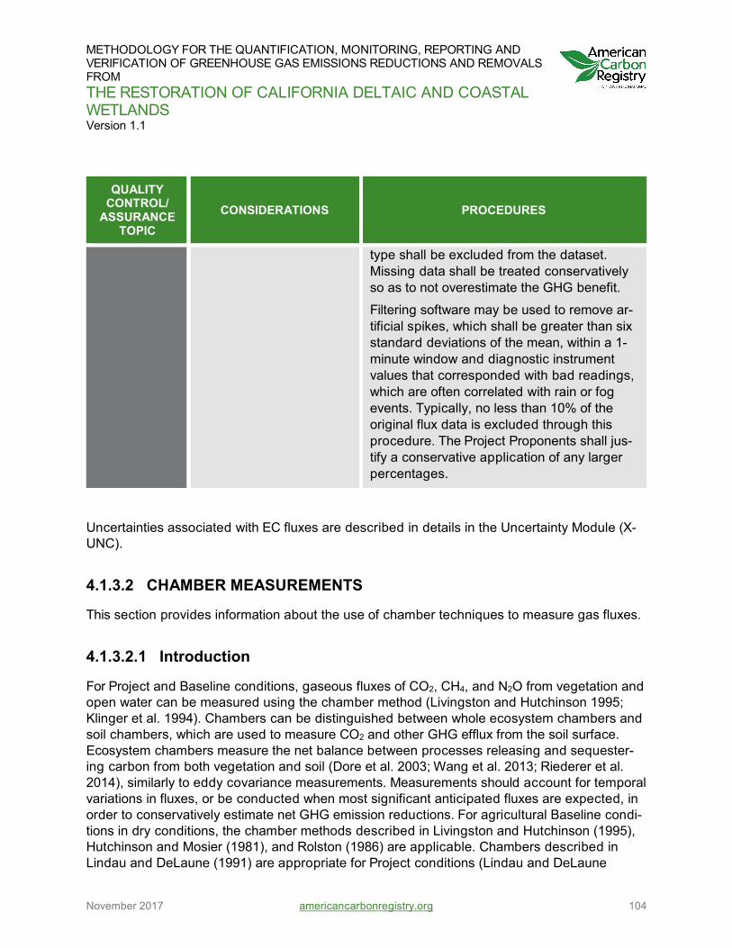
METHODOLOGY FOR THE QUANTIFICATION, MONITORING, REPORTING AND VERIFICATION OF GREENHOUSE GAS EMISSIONS REDUCTIONS AND REMOVALS FROM THE RESTORATION OF CALIFORNIA DELTAIC AND COASTAL WETLANDS Version 1.1
November 2017 americancarbonregistry.org 104
QUALITY CONTROL/
ASSURANCE TOPIC
CONSIDERATIONS PROCEDURES
type shall be excluded from the dataset. Missing data shall be treated conservatively so as to not overestimate the GHG benefit.
Filtering software may be used to remove ar-tificial spikes, which shall be greater than six standard deviations of the mean, within a 1-minute window and diagnostic instrument values that corresponded with bad readings, which are often correlated with rain or fog events. Typically, no less than 10% of the original flux data is excluded through this procedure. The Project Proponents shall jus-tify a conservative application of any larger percentages.
Uncertainties associated with EC fluxes are described in details in the Uncertainty Module (X-UNC).
4.1.3.2 CHAMBER MEASUREMENTS
This section provides information about the use of chamber techniques to measure gas fluxes.
4.1.3.2.1 Introduction
For Project and Baseline conditions, gaseous fluxes of CO2, CH4, and N2O from vegetation and open water can be measured using the chamber method (Livingston and Hutchinson 1995; Klinger et al. 1994). Chambers can be distinguished between whole ecosystem chambers and soil chambers, which are used to measure CO2 and other GHG efflux from the soil surface. Ecosystem chambers measure the net balance between processes releasing and sequester-ing carbon from both vegetation and soil (Dore et al. 2003; Wang et al. 2013; Riederer et al. 2014), similarly to eddy covariance measurements. Measurements should account for temporal variations in fluxes, or be conducted when most significant anticipated fluxes are expected, in order to conservatively estimate net GHG emission reductions. For agricultural Baseline condi-tions in dry conditions, the chamber methods described in Livingston and Hutchinson (1995), Hutchinson and Mosier (1981), and Rolston (1986) are applicable. Chambers described in Lindau and DeLaune (1991) are appropriate for Project conditions (Lindau and DeLaune
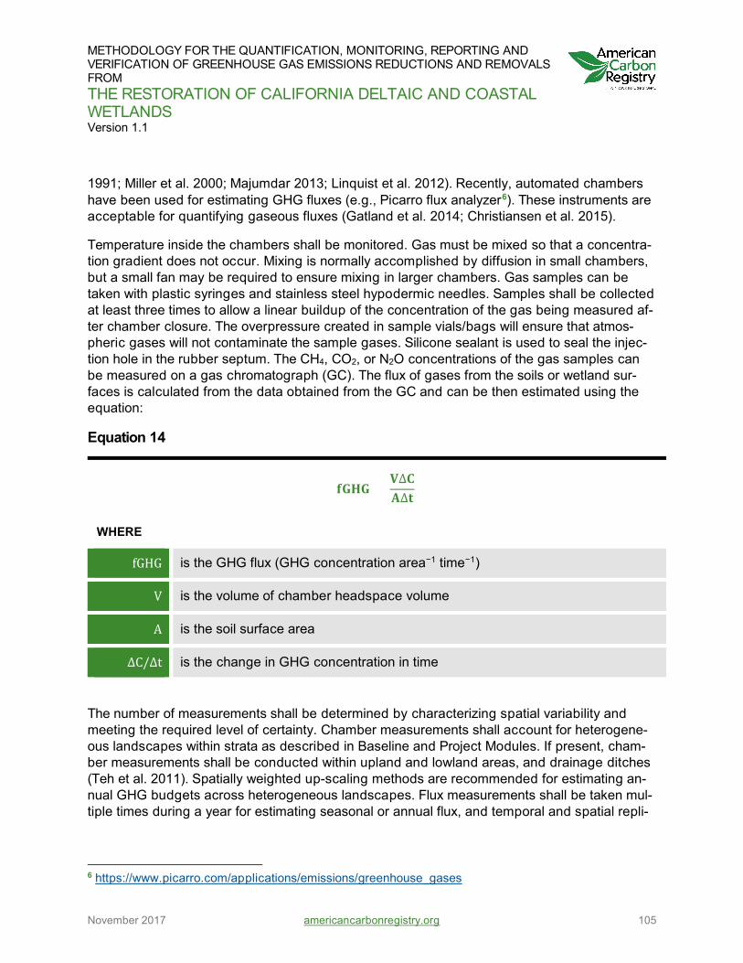
METHODOLOGY FOR THE QUANTIFICATION, MONITORING, REPORTING AND VERIFICATION OF GREENHOUSE GAS EMISSIONS REDUCTIONS AND REMOVALS FROM THE RESTORATION OF CALIFORNIA DELTAIC AND COASTAL WETLANDS Version 1.1
November 2017 americancarbonregistry.org 105
1991; Miller et al. 2000; Majumdar 2013; Linquist et al. 2012). Recently, automated chambers have been used for estimating GHG fluxes (e.g., Picarro flux analyzer6). These instruments are acceptable for quantifying gaseous fluxes (Gatland et al. 2014; Christiansen et al. 2015).
Temperature inside the chambers shall be monitored. Gas must be mixed so that a concentra-tion gradient does not occur. Mixing is normally accomplished by diffusion in small chambers, but a small fan may be required to ensure mixing in larger chambers. Gas samples can be taken with plastic syringes and stainless steel hypodermic needles. Samples shall be collected at least three times to allow a linear buildup of the concentration of the gas being measured af-ter chamber closure. The overpressure created in sample vials/bags will ensure that atmos-pheric gases will not contaminate the sample gases. Silicone sealant is used to seal the injec-tion hole in the rubber septum. The CH4, CO2, or N2O concentrations of the gas samples can be measured on a gas chromatograph (GC). The flux of gases from the soils or wetland sur-faces is calculated from the data obtained from the GC and can be then estimated using the equation:
Equation 14
𝐟𝐟𝐟𝐟𝐟𝐟𝐟𝐟 = 𝐕𝐕∆𝚫𝚫𝐀𝐀∆𝐚𝐚
WHERE
fGHG is the GHG flux (GHG concentration area−1 time−1)
V is the volume of chamber headspace volume
A is the soil surface area
ΔC/Δt is the change in GHG concentration in time
The number of measurements shall be determined by characterizing spatial variability and meeting the required level of certainty. Chamber measurements shall account for heterogene-ous landscapes within strata as described in Baseline and Project Modules. If present, cham-ber measurements shall be conducted within upland and lowland areas, and drainage ditches (Teh et al. 2011). Spatially weighted up-scaling methods are recommended for estimating an-nual GHG budgets across heterogeneous landscapes. Flux measurements shall be taken mul-tiple times during a year for estimating seasonal or annual flux, and temporal and spatial repli-
6 https://www.picarro.com/applications/emissions/greenhouse_gases

METHODOLOGY FOR THE QUANTIFICATION, MONITORING, REPORTING AND VERIFICATION OF GREENHOUSE GAS EMISSIONS REDUCTIONS AND REMOVALS FROM THE RESTORATION OF CALIFORNIA DELTAIC AND COASTAL WETLANDS Version 1.1
November 2017 americancarbonregistry.org 106
cation is important to reduce uncertainty. Boardwalks shall be used for accessing measure-ment sites to prevent disturbance of the marsh surface, soil compaction, and ebullition that would overestimate CH4 fluxes.
Special care must be taken when estimating N2O emissions using chambers. Fertilization and re-wetting events are especially important for N2O budgets, where a single pulse event can ac-count for >50% of the annual N2O budget (Wagner-Riddle et al. 1997). Therefore, in order to accurately estimate N2O emissions using manual chambers, deployment must include fertiliza-tion, irrigation, and precipitation events. These pulse events can encompass several days (1–30 days) and therefore must be evaluated at an appropriate time scale. Estimations of annual N2O budgets from chamber measurements must account for the amount and frequency of ferti-lization, irrigation, and precipitation events in addition to lower-level N2O emission rates that oc-cur outside pulse events.
4.1.3.2.2 Applicability
The following applicability conditions apply to the use of chambers.
The distribution of chamber measurement shall be shown to adequately represent the hydrologic, water quality and soil conditions, and land and water management practices for the stratum.
The monitoring period using chamber measurements shall be sufficient to quantify possible annual variations in GHG fluxes. The Project Proponents shall demonstrate that annual values for GHG fluxes are representative.
When measuring N2O emissions using chambers, deployment must include fertilization, irrigation, and precipitation events.
Monitoring must occur for Baseline establishment and renewal. At least 1 year of monitoring is required for Baseline conditions. Baseline field monitoring should be conducted seasonally for 1 year to determine the seasonal effects on GHG fluxes, or measurements can be made during the period of peak emissions (e.g., summer or fertilization events).
For Project conditions, monitoring is required throughout the life of the Project unless the use of biogeochemical models calibrated with site data are shown to adequately predict GHG fluxes. At this point, chamber measurements may be terminated. For Project conditions, the monitoring frequency shall occur at least every 5 years for 1 year.
4.1.3.2.3 Quality Assurance and Quality Control
Quality assurance and control measures for chamber measurements are listed and discussed in Table 26.

METHODOLOGY FOR THE QUANTIFICATION, MONITORING, REPORTING AND VERIFICATION OF GREENHOUSE GAS EMISSIONS REDUCTIONS AND REMOVALS FROM THE RESTORATION OF CALIFORNIA DELTAIC AND COASTAL WETLANDS Version 1.1
November 2017 americancarbonregistry.org 107
Table 26: Quality Control/Assurance for Chamber Measurements
QUALITY CONTROL/
ASSURANCE TOPIC
CONSIDERATIONS PRECAUTIONS AND SAFE-GUARDS
REFERENCE FOOTNOTE
Temperature Ambient temperature should be preserved within the chamber. So-lar heating of the enclo-sure surface can rap-idly lead to increasing chamber temperatures.
Minimize deployment times, and for soil measurements, use shading of opaque mate-rials, monitor chamber temperature
Livingston and Hutchinson 1995
DEPLOYMENT Development of a disturb-ance-free seal
Leakage can occur in unsaturated-zone soils especially during high winds.
Use weighted skirts around chambers and /or baffled, double-walled enclosures. Avoid high winds. Estimate leakage with a tracer gas.
Livingston and Hutchinson 1995; Crill et al. 1995; Davidson et al. 2002
DEPLOYMENT Surface compaction
Artificial gradients and mass inflow can be in-duced by surface com-paction from foot traf-fic. Water-saturated soils are particularly susceptible.
Use of designated walk-ways, remote gas with-drawal from chambers
Livingston and Hutchinson 1995
DEPLOYMENT Vegetative disturbance
Disturbance of vegeta-tion can affect ex-change processes un-der study and influence plant mediated gas transport
Avoid cutting roots or severing stems and leaves
Crill et al. 1995
Field sample handling and processing
Sample container leak-age and accuracy
Analyze gas samples within a few hours, ana-lyze standards frequently
Crill et al. 1995

METHODOLOGY FOR THE QUANTIFICATION, MONITORING, REPORTING AND VERIFICATION OF GREENHOUSE GAS EMISSIONS REDUCTIONS AND REMOVALS FROM THE RESTORATION OF CALIFORNIA DELTAIC AND COASTAL WETLANDS Version 1.1
November 2017 americancarbonregistry.org 108
QUALITY CONTROL/
ASSURANCE TOPIC
CONSIDERATIONS PRECAUTIONS AND SAFE-GUARDS
REFERENCE FOOTNOTE
Laboratory analysis
Potential for analytical error
Follow acceptable ana-lytical protocol for trace gas analysis
Crill et al. 1995
Flux estima-tion
Time for concentration change measurements, chamber dimensions
Minimize sources of vari-ability in sampling han-dling and analysis using maximum possible measurement period and number of independent samples. Two samples are not sufficient. Deter-mine chamber volume precisely.
Crill et al. 1995
4.1.3.2.4 Equations
Where chambers are used to estimate cumulative GHG emissions, the following equation shall be used.
Equation 15
𝐟𝐟𝐟𝐟𝐟𝐟𝐟𝐟 = �𝟏𝟏𝐞𝐞
× �𝐟𝐟𝐟𝐟𝐟𝐟𝐟𝐟𝐚𝐚𝐞𝐞
𝐚𝐚=𝟏𝟏
�× 𝐄𝐄𝐓𝐓 × 𝚫𝚫𝐁𝐁
WHERE
fGHG is the annual net GHG emissions (MT CO2e)
fGHGt is the rate of GHG emissions from the Project area at monitoring event (MT CO2e per unit of time)
Tp is the time period which corresponds to the annual period (yr)
n is the number of monitoring events

METHODOLOGY FOR THE QUANTIFICATION, MONITORING, REPORTING AND VERIFICATION OF GREENHOUSE GAS EMISSIONS REDUCTIONS AND REMOVALS FROM THE RESTORATION OF CALIFORNIA DELTAIC AND COASTAL WETLANDS Version 1.1
November 2017 americancarbonregistry.org 109
t is the monitoring event
CF is the factor for converting from the measurement time scale to the time scale of Tp
4.1.3.3 HARVESTED GRAIN AND BIOMASS
This section describes methods for quantifying carbon removal from the Project area via har-vested grain and biomass.
4.1.3.3.1 Introduction
The carbon in harvested grain and biomass represents an essential part of the carbon stock changes for Baseline agriculture and rice, or paludiculture Project conditions (Equation 12). Harvested grain or biomass is determined by 1) collection of grain or biomass in representative plots within the stratum; 2) determination of the carbon and moisture content on the collected material using literature and laboratory analysis of the material; and 3) estimation of total car-bon removed in grain and/or biomass for the stratum. Alternatively, the Project Proponent may obtain information from the farmer about the weight of the harvested grain and/or biomass and use literature values and laboratory-determined values for the carbon and moisture content of the harvested grain and/or biomass to estimate the carbon dioxide harvested for the crop for the stratum (MT CO2e) (Equation 16). The moisture content of the harvested material shall be determined at harvest. Methods described in Kalra (1997) and McGeehan and Naylor (1988) are applicable for determination of moisture content and carbon content.
4.1.3.3.2 Applicability
Harvested grain and biomass shall be shown to adequately represent the hydrologic, water quality and soil conditions, and land and water management practices for the stratum.
Annual estimates of harvested grain and biomass are sufficient. For multiple harvests (such as for hay or grain crops), the annual estimate shall equal the sum of all harvests.
Monitoring must occur for Baseline establishment and renewal. For Project conditions, the monitoring frequency shall occur at least every 5 years over a period of 1 year.
The Project Proponent shall demonstrate using maps and photographs that yield plots are representative of the entire stratum.
4.1.3.3.3 Quality Assurance and Quality Control
Where yield plots are used, plots shall be replicated three times within each stratum and the entire plot shall be harvested.

METHODOLOGY FOR THE QUANTIFICATION, MONITORING, REPORTING AND VERIFICATION OF GREENHOUSE GAS EMISSIONS REDUCTIONS AND REMOVALS FROM THE RESTORATION OF CALIFORNIA DELTAIC AND COASTAL WETLANDS Version 1.1
November 2017 americancarbonregistry.org 110
The average yield and standard deviation from the three replicate plots shall be used in uncertainty calculations in the Uncertainty Module (X-UNC).
4.1.3.3.4 Equations
For agricultural Baseline conditions and rice Project conditions, carbon removal in harvested grain and biomass shall be estimated using the following equation (Hollinger et al. 2005):
Equation 16
𝚫𝚫𝐀𝐀𝐚𝐚 = 𝐒𝐒 × 𝐟𝐟𝚫𝚫 × 𝐘𝐘
WHERE
Cgr is the carbon removal in harvested grain and biomass from the Project area (MT CO2e)
W is the moisture content expressed as a fraction
fC is the fraction of carbon in the grain or biomass (Conner and Loomis, 1992)
Y is the yield for the Project area (MT CO2e)
The use of Equation 12 and Equation 16 assumes that 100% of the harvested biomass is even-tually consumed and oxidized to CO2 and CH4 which is released back into the atmosphere.
4.1.3.4 AQUEOUS CARBON LOADS
This section describes quantification of carbon losses and gains at the Project site via aqueous carbon loads.
4.1.3.4.1 Introduction
For Baseline and Project conditions, aqueous carbon loads represent part of the overall carbon budget not explicitly determined by eddy covariance or chambers (Equation 12). Aqueous car-bon can enter and exit the Project area to and from adjacent channels as dissolved and partic-ulate organic carbon. The total organic carbon (TOC) concentration is equal to the sum of par-ticulate and dissolved organic carbon. Loads are equal to the net water flow times the concen-tration of total organic carbon in the water. The Project Proponent shall measure concentra-tions, flow, and loads at the main inlet and outlet of water in Project areas and use methods

METHODOLOGY FOR THE QUANTIFICATION, MONITORING, REPORTING AND VERIFICATION OF GREENHOUSE GAS EMISSIONS REDUCTIONS AND REMOVALS FROM THE RESTORATION OF CALIFORNIA DELTAIC AND COASTAL WETLANDS Version 1.1
November 2017 americancarbonregistry.org 111
published in the peer-reviewed literature for determining concentrations, flow, and loads in tidal (Ganju et al. 2005; Bergamaschi et al. 2011) and non-tidal (Deverel et al. 2007) sys-tems. For flow measurements, methods include manual flow and acoustic velocity me-ters. Methods for total dissolved organic carbon determination in drain-water samples are de-scribed in Deverel et al. (2007). Water management practices that limit drainage from man-aged wetlands substantially limit aqueous carbon exports.
Specifically, for non-tidal managed wetlands, subsurface and surface drainage flow shall be measured and calculated continuously using traditional flow measurements using manually op-erated flow meters and tracking stage at a control device such as a weir with a water level re-corder. Alternatively, flows can be measured using continuous recording acoustic Doppler technology. For tidal systems, a similar approach can be used except that flow is bidirectional depending on tidal influences.
4.1.3.4.2 Applicability
The determination of aqueous carbon loads shall be shown to adequately represent the hydrologic, water quality and soil conditions, and land and water management practices for the stratum.
Measurements shall adequately represent the temporal variability in concentrations and loads.
For non-tidal systems, the temporal variability is determined by hydrologic management and season variability. Monthly measurements are generally sufficient to characterize the temporal variability.
Tidal fluxes of dissolved and particulate organic carbon shall be estimated or measured at intervals that adequately represent temporal variability, as determined by a sensitivity analysis made using the Uncertainty Module.
4.1.3.4.3 Quality Assurance and Quality Control
The uncertainty in manual flow measurements shall be determined as per the guidance in Sauer and Meyer (1992) and incorporated into the uncertainty equations in the Uncertainty Module (X-UNC). Uncertainty in acoustic velocity measurements shall be evaluated using infor-mation described in Laenen and Curtis (1989). Analytical uncertainty for dissolved organic car-bon shall be determined using field duplicate and blank samples and laboratory QA/QC sam-ples, and shall be incorporated into the flow measurement uncertainty.
4.1.3.4.4 Equations
The annual net aqueous loss of dissolved and particulate organic carbon (Eaq, in Equation 12) can be calculated by subtracting the aqueous carbon input from the aqueous carbon export. Specifically,

METHODOLOGY FOR THE QUANTIFICATION, MONITORING, REPORTING AND VERIFICATION OF GREENHOUSE GAS EMISSIONS REDUCTIONS AND REMOVALS FROM THE RESTORATION OF CALIFORNIA DELTAIC AND COASTAL WETLANDS Version 1.1
November 2017 americancarbonregistry.org 112
Equation 17
𝐄𝐄𝐚𝐚𝐄𝐄 = (𝐐𝐐𝐀𝐀𝐞𝐞𝐓𝐓𝐞𝐞𝐚𝐚𝐚𝐚 × [𝐄𝐄𝐎𝐎𝚫𝚫] −𝐐𝐐𝐞𝐞𝐞𝐞𝐓𝐓𝐞𝐞𝐚𝐚𝐚𝐚 × [𝐄𝐄𝐎𝐎𝚫𝚫])
WHERE
Qexport water flow exiting the Project area
Qimport water flow entering the Project area
[TOC] is the total organic carbon concentration, sum of particulate and dissolved organic carbon
Allochthonous carbon may enter a Project area from an outside source and may contribute to carbon accumulation at the site. However, it represents carbon assimilated by other sinks and the wetland Project area does not contribute to its removal from the atmosphere. For this rea-son, after it is quantified (as described in Equation 12), if a project area receives an input of al-lochthonous carbon, it should be deducted from the total carbon stock change of the Project area. For purposes of this methodology, carbon accumulation from outside sources may be ex-cluded in determination of Baseline or Project GHG emissions or removals if not significant as per guidance of tool T-SIG. Allochthonous carbon accumulation in the Baseline may be con-servatively set to zero, as its exclusion from the balance between GHG losses and gains would underestimate total GHG emission reductions. In the Project Scenario, net accumulation of al-lochthonous carbon must be subtracted from the net carbon balance of a wetland unless the Project Proponent can document that no other entity may claim its GHG emission reductions or removals (i.e., that no other entity may make an ownership claim to the emission reductions or removals for which credits are sought) and if its storage in the tidal wetland decreases the rate of its decomposition compared to what it would be in the absence of the Project (i.e., the case the tidal wetland was not implemented). In the Baseline Scenario, net accumulation of alloch-thonous carbon must be accounted for and subtracted from the baseline total carbon stock change, or can be conservatively set to zero.
4.1.3.5 SUBSIDENCE MEASUREMENTS
This section describes methods and techniques for subsidence measurements.
4.1.3.5.1 Introduction
For purpose of this methodology, subsidence is caused by the oxidation of organic soils (Deverel and Leighton 2010). As organic soils are drained for agricultural use and exposed to

METHODOLOGY FOR THE QUANTIFICATION, MONITORING, REPORTING AND VERIFICATION OF GREENHOUSE GAS EMISSIONS REDUCTIONS AND REMOVALS FROM THE RESTORATION OF CALIFORNIA DELTAIC AND COASTAL WETLANDS Version 1.1
November 2017 americancarbonregistry.org 113
oxygen, they oxidize and disappear. Subsidence is estimated as the difference between eleva-tions at two points in time. Subsidence measurements, when the soil carbon pool includes bio-mass and dead organic matter of non-woody annual vegetation, can represent the ecosystem carbon stock changes. For example, Couwenberg et al. (2013) described a simple approach to determining total ecosystem net carbon loss from subsidence records.
If subsidence measurements are used, it is assumed that the soil carbon pool includes all eco-system carbon pools. Where there are elevation measurements in organic or highly organic mineral soils at two or more points in time, the difference in elevation and soil carbon density can be used to estimate historic Baseline emissions by multiplying the elevation change by the soil carbon density. Soil carbon density is equal to the soil carbon content multiplied by the soil bulk density. Data for soil organic matter content for Delta and San Francisco Bay Estuary soils is described in Callaway et al. (2012), Deverel and Leighton (2010), and Drexler et al. (2009). Soil carbon content is generally equal to 50% of the soil organic matter content. Drexler et al. (2009) provided data for soil bulk density for eight Delta islands. Caution should be exercised and uncertainty quantified when using the relations of bulk density and organic matter and car-bon and organic matter where they have not been verified using Project data.
4.1.3.5.2 Applicability
The number of measurements shall be determined by strata, known spatial variability, and the required level of certainty as per the guidance in the T-PLOT tool. The determination of subsidence shall be shown to adequately represent the hydrologic, water quality and soil conditions, and land and water management practices for the stratum.
Project Proponents shall be conservative in estimating the depth of subsidence from elevation measurement differences by calculating the minimum possible difference between elevations measured at two points in time.
All elevation measurements for subsidence calculations shall be referenced to stable benchmarks.
Project Proponents shall ensure and document the consistent use of vertical datums for elevations measured during different years.
Project Proponents shall use conservative values for soil organic carbon and bulk density values that result in conservative estimates for subsidence.
4.1.3.5.3 Quality Assurance and Quality Control
Uncertainty in subsidence estimates stem from 1) elevation measurements; and 2) soil carbon and bulk density determinations. For elevation measurements, uncertainty is dependent on methods used that shall be documented and incorporated into uncertainty calculations in the Uncertainty Module (X-UNC). For example, Deverel and Leighton determined elevations at lo-cations on Bacon Island in 2006 where elevations were measured by University of California researchers in 1978. The vertical closure error (the amount by which an elevation determined

METHODOLOGY FOR THE QUANTIFICATION, MONITORING, REPORTING AND VERIFICATION OF GREENHOUSE GAS EMISSIONS REDUCTIONS AND REMOVALS FROM THE RESTORATION OF CALIFORNIA DELTAIC AND COASTAL WETLANDS Version 1.1
November 2017 americancarbonregistry.org 114
by a series of elevation measurements fails to agree with an established elevation) for the 1978 survey with traditional surveying equipment was 0.07 meters (m). For the 2006 survey, which utilized real-time kinematic, static, and fast-static Global Positioning System measurements, vertical closure error was 0.002 m. Therefore, the conservatively estimated subsidence at any point along the survey route followed in 1978 and 2006 is equal to the elevation determined in 1978 minus the closure error, minus the sum of 2006 elevation and the closure error. Table 27 shows an example calculation. Elevation errors in topographic-map elevations range from about 0.3 to 1 m.
Table 27: Example Subsidence Calculation for Point 44027 on Figure 2 in Deverel and Leighton
YEAR ELEVATION (M)
CLOSURE ERROR (M)
DEPTH OF SUBSIDENCE (M)
1978 -3.98 0.07 No subsidence – Time series begins
2006 -5.26 0.002 1.21 ((-3.98 – 0.07) - (-5.26+0.002))
Data presented in Drexler et al. (2009) provide ranges of estimates for organic matter content and bulk density for eight Delta islands.
4.1.3.5.4 Equations
When the cumulative net Baseline carbon stock changes and GHG emissions for the Project area can be estimated by changes in the soil carbon pools using the depth of subsidence, the following equation can be used:
Equation 18
𝚫𝚫𝚫𝚫𝐁𝐁𝐁𝐁𝐁𝐁 =𝟎𝟎𝟎𝟎𝟏𝟏𝟐𝟐
× �(𝐁𝐁𝐞𝐞
𝐞𝐞
𝐞𝐞=𝟏𝟏
× 𝐁𝐁𝐁𝐁𝐞𝐞 × 𝐟𝐟𝚫𝚫𝐞𝐞 × 𝐀𝐀𝐞𝐞 )
WHERE
S is the depth of land subsidence (m)
BD is the dry bulk density of the organic soil (t m-3)
fC is the fraction of carbon in the organic soil on a dry weight basis

METHODOLOGY FOR THE QUANTIFICATION, MONITORING, REPORTING AND VERIFICATION OF GREENHOUSE GAS EMISSIONS REDUCTIONS AND REMOVALS FROM THE RESTORATION OF CALIFORNIA DELTAIC AND COASTAL WETLANDS Version 1.1
November 2017 americancarbonregistry.org 115
44/12 is the ratio of molecular weights of CO2 to carbon (dimensionless)
A is the area of the stratum (m2)
i refers to the stratum within the Project boundary
n is the number of strata within the Project boundary
4.1.3.6 SOIL CORING, SEDIMENT EROSION TABLES, AND SEDIMENT PINS
The following sections describe methods used for soil carbon determination via soil sampling.
4.1.3.6.1 Introduction
Carbon stock changes in the soil carbon pool in managed non-tidal wetlands and tidal wet-lands can be measured in soil cores by determining the carbon accumulated above feldspar markers or sediment pins pounded into the ground to refusal (US Geological Survey 2012) placed at the start of Project activities. Sedimentation erosion tables (SET) can also be used to determine soil biomass accretion. Sediment pins are subject to greater uncertainty than sedi-ment erosion tables. Sediment pins are generally applicable where the depths of accretion are greater than 10 to 20 cm. Localized scour around sediment pins can occur. Experience in the San Francisco Bay Estuary demonstrates that basing measurements on the broader sediment surface can provide the necessary accuracy. The material located above the feldspar marker or sediment pin/sediment interface or at the SET measurement plot shall be analyzed for total carbon or organic matter content and bulk density. Any compaction that occurs should be measured and accounted for. The change in carbon stocks in soil cores shall be determined by quantifying the carbon density above a marker horizon defined by a feldspar marker.
Feldspar markers should be placed at the start of the Project activity. Feldspar marker horizons are prepared by spreading a thin aqueous slurry (~1 cm) layer of feldspar clay on the wet-land surface (Cahoon and Turner 1989). Soil carbon content can be determined using ele-mental analysis using a CHN analyzer (Nelson and Sommers 1982) or estimated from the loss-on-ignition method (LOI) (Ball 1964). Results throughout the Sacramento-San Joaquin Delta and San Francisco Bay Estuary (Drexler et al. 2009; Callaway et al. 2012; Craft et al. 1991) demonstrate a statistically significant relation between soil carbon content and LOI. These regression relations can be used to calculate the carbon content of the harvested cores on a mass carbon per mass of soil basis. A weak regression would generate high uncer-tainty in the estimate. As for any variable included in the protocol, Project Proponents should strike a balance between the reduction of the Emission Reduction Tons (ERT) caused by ele-vated uncertainty and the costs needed to reduce such uncertainty.

METHODOLOGY FOR THE QUANTIFICATION, MONITORING, REPORTING AND VERIFICATION OF GREENHOUSE GAS EMISSIONS REDUCTIONS AND REMOVALS FROM THE RESTORATION OF CALIFORNIA DELTAIC AND COASTAL WETLANDS Version 1.1
November 2017 americancarbonregistry.org 116
To estimate carbon density in mass per unit volume, multiply the carbon content and the bulk density. The bulk density shall be determined using methods reported in Calloway et al. (2012) and Blake (1965).
Specific steps for core collection:
Step 1 Collect soil core samples and measure the depth of the feldspar marker or measure the sediment accumulated at the sediment pin, and collect a soil core sample to the depth of accumulated sediment. See the Quality Assurance section below for discussion of compaction and compaction avoidance.
Step 2 Multiple samples collected at the same plot may be aggregated provided that the uncertainty and guidance for estimating the appropriate number of samples is documented.
Step 3 For bulk density analysis, a single core shall be collected next to the core collected for determination of soil carbon content. Soil samples need to be thoroughly dried until their weight no longer changes and then the weight of each section needs to be divided by the volume.
Step 4 The mass of carbon per unit volume is calculated as the product of the carbon concentration and bulk density.
Sedimentation erosion tables (SET) and rod sedimentation erosion tables (RSET) may be used to determine the accumulation of biomass with time in conjunction with coring and determina-tion of the mass of carbon per unit volume of the accumulating material (Lynch 2015). Addi-tional guidance for estimating carbon stock changes and GHG emissions for tidal wetlands and sea grasses is provided by Howard et al. (2014).
4.1.3.6.2 Applicability
The number of samples shall be determined by strata, known spatial variability, and the re-quired level of certainty, as outlined in the T-PLOT tool. The determination of soil carbon stock changes shall be shown to adequately represent the hydrologic, water quality and soil condi-tions, and land and water management practices for the stratum.
4.1.3.6.3 Quality Assurance and Quality Control
The primary quality control/quality considerations are related to 1) accurate depth of the core; and 2) spatial variability. Compaction during core collection is estimated by measuring the dif-ference in elevation inside and outside of the coring tube to the nearest millimeter. Example coring devices include McAuley (Bricker-Urso et al. 1989), Livingstone (Wright 1991), or Hargis

METHODOLOGY FOR THE QUANTIFICATION, MONITORING, REPORTING AND VERIFICATION OF GREENHOUSE GAS EMISSIONS REDUCTIONS AND REMOVALS FROM THE RESTORATION OF CALIFORNIA DELTAIC AND COASTAL WETLANDS Version 1.1
November 2017 americancarbonregistry.org 117
(Hargis and Twilley 1994) coring devices, which allow cores to be taken with minimal or no compaction. Strata and known spatial variability shall determine the number of samples and the required level of certainty as described in the T-PLOT tool.
If inorganic carbon is present in soil samples, there may be interference in the determination of soil organic carbon. Total inorganic carbon can be determined and subtracted from the or-ganic carbon determination.
4.1.3.6.4 Equations
Soil coring is used to estimate soil carbon stock changes. To estimate the change in soil car-bon (ΔCsoil) for the Project area during the reporting period (MT CO2e)
Equation 19
∆𝚫𝚫𝐀𝐀𝐞𝐞𝐞𝐞𝐚𝐚 =𝟏𝟏𝐔𝐔
× �(𝐁𝐁𝐞𝐞
𝐞𝐞
𝐞𝐞=𝟏𝟏
× 𝚫𝚫𝐁𝐁𝐞𝐞)
WHERE
Di is the depth of the soil accumulated above a feldspar marker
CDi is the carbon density of the soil accumulated above a feldspar marker (product of the soil carbon content on a weight basis and soil bulk density)
i is the stratum within the Project boundary
N is the number of cores collected with stratum
4.1.3.7 BIOMASS CARBON POOLS AND BIOGEOCHEMICAL MODEL INPUTS
When methods described in this section are used to determine carbon stock changes, the Pro-ject Proponents shall demonstrate that the estimated GHG removal by above- and below-ground biomass is not already included in the determination of the overall carbon stock change calculation.
Rates of carbon accumulation in above and below-ground biomass can be measured using:
direct measurements (allometric determinations and harvesting) indirect methods (remote sensing and other techniques)

METHODOLOGY FOR THE QUANTIFICATION, MONITORING, REPORTING AND VERIFICATION OF GREENHOUSE GAS EMISSIONS REDUCTIONS AND REMOVALS FROM THE RESTORATION OF CALIFORNIA DELTAIC AND COASTAL WETLANDS Version 1.1
November 2017 americancarbonregistry.org 118
Litter decomposition can be estimated using:
traditional litterbags isotopic analysis modeling
4.1.3.7.1 Estimating Above- and Below-Ground Biomass Using Allometric and Destructive Methods
The mean carbon stock in above- and below-ground biomass per unit area is estimated based on field measurements of the wetland plants in fixed area plots using allometric equations and destructive methods such as those described in Miller and Fujii (2010) and Howard et al. (2014) (Table 28). The number and size of plots shall ensure adequate representation of the area being measured by utilizing guidance provided in the T-PLOTS tool. The allometric method can be used to estimate above-ground biomass by using equations that express above-ground biomass as a function of plant height and diameter. For example, Miller and Fujii (2010) used extensive destructive biomass harvest to determine parameters in allometric equations for the predominant species (Typha and Schoenoplectus spp) in managed non-tidal wetlands in the Delta. The following table provides the equations from Miller and Fujii (2010).
Table 28: Allometric Equations for Above-Ground Biomass Estimates (in g Dry Weight m-2)
SPECIES DESCRIPTION EQUATION
Schoenoplectus acutus
Biomass weight using height and diameter
log10weight = (0.5028 x ln height) + (0.3471 x ln diameter) - 1.7654
r2 = 0.924
Schoenoplectus acutus
Biomass weight using only height
log10weight = (0.7947 * ln height) - 3.2177
r2 = 0.824
Typha species
Plant biomass weight using height, diameter and leaf number
log10weight = -2.188 + (0.601 x ln height) + (0.2128 x ln diameter) + (0.2721 x ln leaf number) - 0.484
r2 = 0.9

METHODOLOGY FOR THE QUANTIFICATION, MONITORING, REPORTING AND VERIFICATION OF GREENHOUSE GAS EMISSIONS REDUCTIONS AND REMOVALS FROM THE RESTORATION OF CALIFORNIA DELTAIC AND COASTAL WETLANDS Version 1.1
November 2017 americancarbonregistry.org 119
Miller and Fujii reported root biomass measurements and root:shoot ratios ranging from 0.6 ± 0.2 to 1.7 ± 0.4 for Schoenoplectus acutus and 0.7 ± 0.1 to 1.0 ± 0.3 for Typha sp. Values var-ied seasonally and with water depth. Average values for both species were not significantly dif-ferent; 0.9 ± 0.1 for Schoenoplectus acutus and 0.8 ± 0.1 for Typha sp. For the purposes of this methodology for constructed wetland activities where these species are present, these val-ues are appropriate for multiplication times the above-ground biomass weight. Destructive methods such as those described in Miller and Fujii can also be used to determine root bio-mass.
Where there are trees, methods described in Howard et al. (2014) can be used to estimate car-bon stocks.
4.1.3.7.2 Estimating Biomass Using Remote Sensing Methods
Spectral information from remotely sensed imagery can be used to estimate above-ground bio-mass accumulating during the year. This spectral information can be used to not only estimate above-ground biomass, but also the fraction of photosynthetically active material driving photo-synthesis, as well as the timing and duration of the growing season. This information can used as input for the biogeochemical model for wetlands described below.
PHENOCAM. Phenocams are digital cameras that are automated to record images of canopy cover throughout the year. These images can then be processed to calculate a greenness in-dex (GI) that can be empirically related to above-ground leaf area index (LAI) based on field measurements, where LAI is defined as half the total developed area of green leaves per unit ground surface area. LAI can be directly measured using destructive field sampling or meas-ured using a LAI sensor such as the LAI-2200C Plant Canopy Analyzer (LI-COR, Lincoln, NE, USA) (Sonnentag et al. 2011). Measurements must be collected several times during the grow-ing season. LAI is an input to biogeochemical models and can be used to estimate gross pri-mary productivity for Project conditions (managed and tidal wetlands and rice).
SATELLITE IMAGES. Satellite-derived LAI products give information across large spatial scales (e.g., 1km for MODIS) with fairly high temporal resolution (e.g., 8–16 days for MODIS). The drawbacks to this method include poor small-scale resolution associated with high uncertainty at the field scale as well as data gaps associated with cloud cover (Garrigues et al. 2008). Sat-ellite-derived LAI products are therefore ideal for projects encompassing large spatial scales (multiple square kilometers) and need to be supplemented with direct measurements. Addi-tional guidance for use of remote sensing is provided in Howard et al. (2014).
Project Proponents should be aware that standing dead materials can persist in non-tidal marshes for multiple years, which can influence remotely sensed estimates of leaf-area indices and biomass as live shoot density decreases in areas with dense thatch.

METHODOLOGY FOR THE QUANTIFICATION, MONITORING, REPORTING AND VERIFICATION OF GREENHOUSE GAS EMISSIONS REDUCTIONS AND REMOVALS FROM THE RESTORATION OF CALIFORNIA DELTAIC AND COASTAL WETLANDS Version 1.1
November 2017 americancarbonregistry.org 120
4.1.3.7.3 Estimating Litter Decomposition
Litter decomposition represents a large term in the global carbon budget, playing a critical role in regulating soil carbon dynamics across multiple scales of space and time (Zhang et al. 2008). Determination of litter decomposition rates is used in biogeochemical models that esti-mate soil CO2 emissions. Project Proponents shall avoid double-counting when using decom-position or accumulation of litter in Project GHG accounting and soil carbon stock changes or other flux measurements already account for these processes. To accurately predict litter car-bon stock changes, litter decomposition rates (k) must be measured or estimated. Litterbags are the most widely used method for direct k calculations and have been used and replicated around the world for decades (Olson 1963) and can be used within this methodology. The analysis of natural abundances of 13C isotopes (Silva et al. 2013), as well as labeling experiments with isotopically enriched litter (Qiao et al. 2014), are also effective ways to esti-mate litter carbon stock changes over time. Laboratory microcosm studies show large discrep-ancy in relation to field litterbag and isotopic studies and shall not be used. Modeled decom-position rates on the long-term inter-site decomposition experiment team (LIDET) (Bonan et al. 2013) can be used to provide conservative estimates of decomposition.
Predicting root decomposition at wetland sites is greatly improved by estimating decomposi-tion rates of wetland roots separately from all other litter. The LIDET databases can be used to generate conservative root decomposition estimates. The same methods shall be employed to estimate k values under Baseline and Project conditions. If models are used, they shall be con-strained by main drivers of decomposition, such as geographic factors (latitude and altitude), climatic factors (temperature, precipitation, evapotranspiration), and litter quality (C:N ratios, lignin content), and calibrated using data for the Project or demonstrably equivalent conditions.
4.2 (MODEL-W/RC) BIOGEOCHEMICAL MODELS
4.2.1 Scope Biogeochemical models allow for the ex-ante and ex-post estimation of GHG removals and emissions.
To be used by the Project Proponents, models must meet the following requirements:
Be documented in the peer-reviewed literature; Be validated in the Project area or similar sites using peer-reviewed or other quality
controlled data (i.e., collected as part of a government soils inventory or experiment) for the soils and for the hydrologic and biogeochemical conditions in the proposed Project area;
Be calibrated using peer-reviewed or other quality-controlled parameter appropriate to each identified stratum;

METHODOLOGY FOR THE QUANTIFICATION, MONITORING, REPORTING AND VERIFICATION OF GREENHOUSE GAS EMISSIONS REDUCTIONS AND REMOVALS FROM THE RESTORATION OF CALIFORNIA DELTAIC AND COASTAL WETLANDS Version 1.1
November 2017 americancarbonregistry.org 121
Be able to effectively simulate carbon stock changes and GHG emissions for Baseline and Project conditions;
For models that include litter, above- and below-ground biomass, and soil organic matter pools, be able to demonstrate that there is no double-counting of carbon pools and include consideration of conservativeness and significance testing;
Be conservative in estimating GHG emission reductions.
For Project conditions, a validated process-based biogeochemical model, the Peatland Eco-system Photosynthesis, Respiration, and Methane Transport model (PEPRMT, pronounced “peppermint,” also referred to as LUE-DAMM [Oikawa et al. 2017]), can be used for ex-ante estimation of CO2 and CH4 exchange from wetlands in the Sacramento-San Joaquin Delta (see Appendix C).
For agricultural Baseline conditions in the Sacramento-San Joaquin Delta, the SUBCALC model (Deverel and Leighton 2010) may be used to estimate Baseline CO2 emissions (see Ap-pendix C).
Additional models have been used to predict elevation changes in coastal ecosystems. The WARMER model (Wetland Accretion Rate Model of Ecosystem Resilience (Swanson et al. 2014) is a 1-D model of elevation that incorporates both biological and physical processes of vertical marsh accretion. The MEM model (Marsh Equilibrium Model) was developed as a tool for forecasting the future lifespan of coastal wetlands in the face of sea level rise. It forecasts marsh productivity and relative elevation (http://129.252.139.114/model/marsh/mem.asp).
4.2.2 Applicability and Methodological Requirements The following conditions must be met for this Module to be used:
For Project areas that are converted to flooded conditions, separate model simulations must be run for Baseline and Project conditions.
The participating wetlands shall be in areas where the models have been successfully calibrated.
The model is applicable to fully vegetated wetlands or strata. Wetlands or strata with open water require separate validation.7 Net aqueous loss of carbon must be included in the model, be insignificant, or be estimated
using other methods (see Methods Module MM-W/RC and T-SIG tool). For each model run, appropriate input parameter files must be available to the verifier.
7 Conditions 3 and 4 represent different conditions that may occur in the same wetland or stratum due to
hydrologic conditions or the stage of development.

METHODOLOGY FOR THE QUANTIFICATION, MONITORING, REPORTING AND VERIFICATION OF GREENHOUSE GAS EMISSIONS REDUCTIONS AND REMOVALS FROM THE RESTORATION OF CALIFORNIA DELTAIC AND COASTAL WETLANDS Version 1.1
November 2017 americancarbonregistry.org 122
PARAMETERS
PARAMETER SI UNIT DESCRIPTION
ΔCBSL MT CO2e Cumulative total of carbon stock changes and GHG emissions for the Baseline Scenario. This parameter feeds into Equation 1 in the Methodology Framework Module (MF-W/RC).
ΔCactual
MT CO2e Cumulative total of carbon stock changes and GHG emissions for the Project Scenario. This parameter feeds into Equation 1 in the Methodology Framework Module (MF-W/RC).
4.2.3 Model Calibration and Validation In order to use a biogeochemical model, it needs to be parameterized, calibrated and vali-dated for a specific Scenario, Project type, and area. Project emissions of CO2 and CH4 and N2O may be estimated using biogeochemical models, which must be run separately for each site, stratum, or cohort. The biogeochemical model must be parametrized and calibrated for each stratum of each scenario (BL-AG, BL-SW, BL-OP, PS-MW, PS-TW, PS-RC) and for the specific characteristics of vegetation, soil, climate, hydrology of the stratum. Biogeochemical models must be validated for each GHG gas, verification period and stratum. If a range of con-dition exists among strata, the model can be validated only in the most diverse and extreme strata (for example highest and lowest soil organic matter, vegetation cover etc.). Validation within project boundary is not required if it is shown that the biogeochemical model can repro-duce GHG fluxes for the range of conditions existing in the region, and that the condition range includes specific conditions existing at each stratum/site (different soil types, climate, water depth and salinity, vegetation cover, vegetation types).
Model calibration,parameterization and validation should preferably use at least 2 years of eco-system flux data of CO2 and CH4. Other model input variables will also need to be recorded during this time. Based on experience, 2 years is the minimum in order for sufficient data for both parameterization and validation (recommended 70% data used for parameterization and 30% for validation). Also, the model may be calibrated with monitoring data collected after Pro-ject commencement. If discontinuous data are collected and used for calibration, model uncer-tainty will likely be greater and need to be quantified as per guidance in the Uncertainty Mod-ule (X-UNC).

METHODOLOGY FOR THE QUANTIFICATION, MONITORING, REPORTING AND VERIFICATION OF GREENHOUSE GAS EMISSIONS REDUCTIONS AND REMOVALS FROM THE RESTORATION OF CALIFORNIA DELTAIC AND COASTAL WETLANDS Version 1.1
November 2017 americancarbonregistry.org 123
4.3 (E-FFC) METHODS TO ESTIMATE FOSSIL FUEL EMISSIONS
Project Proponents will employ the currently approved Methods Module for estimating GHG emissions fossil fuel combustion approved by ACR.8
The fossil fuel emissions Methods Module shall be used to estimate all Project emissions that include but are not limited to earth-moving, construction, and agricultural operations such as cultivation, planting, and harvesting.
Annual emission estimate (EFFC) in the Module E-FFC are cumulated to obtain the total fossil fuel Emission fEFF for the Project area during the reporting period (t = year):
Equation 20
𝐟𝐟𝐄𝐄𝐁𝐁𝐁𝐁 = � 𝐄𝐄𝐁𝐁𝐁𝐁𝚫𝚫𝟎𝟎𝟎𝟎
𝐚𝐚=𝟏𝟏
A Wetland Project will typically include higher fossil fuel emissions for the initial phase of imple-mentation of the project, and then lower (or zero) levels of fossil fuel emissions for the rest of the crediting period. The total fEFF for the Crediting period can be divided by the number of years (40) to obtain an annualized emissions rate to use to calculate ERT for each verification period.
4.4 (X-UNC) METHODS FOR ESTIMATING UNCERTAINTY
4.4.1 Scope This Module provides guidance for calculating uncertainty for estimation of emissions and GHG removals from wetland construction and restoration activities and rice cultivation activi-ties.
8 E-FFC-WR Module, Estimation of emissions from fossil fuel combustion, in the methodology “Restora-
tion of Degraded Deltaic Wetlands of the Mississippi Delta.”

METHODOLOGY FOR THE QUANTIFICATION, MONITORING, REPORTING AND VERIFICATION OF GREENHOUSE GAS EMISSIONS REDUCTIONS AND REMOVALS FROM THE RESTORATION OF CALIFORNIA DELTAIC AND COASTAL WETLANDS Version 1.1
November 2017 americancarbonregistry.org 124
4.4.2 Applicability This Module is mandatory and provides guidance for the calculation of the following sources of uncertainty:
Baseline and Project emissions Baseline and Project changes in carbon stocks
Where an uncertainty value is unknown, or cannot be accurately calculated, a Project Propo-nent can use an indisputably conservative value for carbon stock changes or GHG emissions, in which case an uncertainty of 0% may be used for this component.
4.4.3 Parameters This Module provides procedures to determine uncertainties.
PARAMETER DESCRIPTION
UNC Total (Project and Baseline) uncertainty (%)
UNCBSL Percentage uncertainty of the combined carbon stocks and GHG fluxes for the Baseline Scenario
UNCP Percentage uncertainty of the combined carbon stocks and GHG fluxes for the Project Scenario
Either IPCC Guidelines for GHG inventories (Eggleston et al. 2006; Penman et al. 2003), expert judgment,9 or estimates based on sound sampling design and statistical analysis shall provide the basis for uncertainty calculations. Uncertainties arising from the measurement of carbon pools changes and GHG fluxes shall always be quantified.
To calculate total Project Uncertainty, the following equation shall be applied:
Equation 21
𝐄𝐄𝐞𝐞𝐚𝐚𝐚𝐚𝐚𝐚 (𝐏𝐏𝐚𝐚𝐞𝐞𝐀𝐀𝐀𝐀𝐚𝐚𝐚𝐚 𝐚𝐚𝐞𝐞𝐀𝐀 𝐁𝐁𝐚𝐚𝐀𝐀𝐀𝐀𝐚𝐚𝐞𝐞𝐞𝐞𝐀𝐀) 𝐔𝐔𝐔𝐔𝚫𝚫 = �𝐔𝐔𝐔𝐔𝚫𝚫𝐁𝐁𝐁𝐁𝐁𝐁𝟐𝟐 + 𝐔𝐔𝐔𝐔𝚫𝚫𝐏𝐏𝟐𝟐
9 Justification should be supplied for all values and parameters measured or derived from expert judg-
ment.

METHODOLOGY FOR THE QUANTIFICATION, MONITORING, REPORTING AND VERIFICATION OF GREENHOUSE GAS EMISSIONS REDUCTIONS AND REMOVALS FROM THE RESTORATION OF CALIFORNIA DELTAIC AND COASTAL WETLANDS Version 1.1
November 2017 americancarbonregistry.org 125
WHERE
UNC is the total (Project and Baseline) uncertainty (%)
UNCBSL is the Baseline uncertainty (%)
UNCP is the Project uncertainty (%)
The allowable uncertainty under this methodology is ±10% of the mean carbon stock change at the 90% confidence level. Where this precision level is met, no deduction shall result for un-certainty. Where uncertainty exceeds 10% of the mean carbon stock change, the deduction shall be equal to the amount that the uncertainty exceeds the allowable level, as indicated in the Methodology Framework Module (MF-W/RC).
4.4.4 Estimating Baseline Uncertainty It is important that the process of Project planning consider uncertainty. A priori estimations of statistical power (Park 2010) can be used to ensure proper spatiotemporal replication (Silva et al. 2013) and determine procedures, such as stratification and allocation of resources to allow the number of measurement plots to reduce uncertainty. It is good practice to consider uncer-tainty at an early stage to identify the data sources with the highest risk to allow the opportunity to conduct further work to improve representativeness and optimize Project practices over time. Estimation of uncertainty for pools and emissions sources requires calculation of both the mean and the 90% confidence interval. In all cases, uncertainty should be expressed as per-centage as the 90% confidence interval of the mean.
The uncertainty in the Baseline Scenario is defined as the square root of the summed errors in each of the carbon pools and GHG fluxes listed in the Baseline Modules for each stratum. For modeled results, the uncertainty in the input inventory data and model structural uncertainty shall be considered as discussed below. The total Baseline uncertainty in each pool or GHG flux can be weighted by the size of the pool or GHG flux and the contribution of each stratum, so that Projects may reasonably target a lower precision level for pools that comprise only a small proportion of the total stock as follows:
Equation 22
𝐔𝐔𝐞𝐞𝐚𝐚𝐀𝐀𝐚𝐚𝐚𝐚𝐚𝐚𝐞𝐞𝐞𝐞𝐚𝐚𝐲𝐲𝐁𝐁𝐁𝐁𝐁𝐁,𝐁𝐁𝐁𝐁,𝐞𝐞 =�(𝐔𝐔𝐁𝐁𝐁𝐁𝐁𝐁,𝐁𝐁𝐁𝐁𝟏𝟏,𝐞𝐞 × 𝐄𝐄𝐁𝐁𝐁𝐁𝐁𝐁,𝐁𝐁𝐁𝐁𝟏𝟏,𝐞𝐞)𝟐𝟐 + (𝐔𝐔𝐁𝐁𝐁𝐁𝐁𝐁,𝐁𝐁𝐁𝐁𝟐𝟐,𝐞𝐞 × 𝐄𝐄𝐁𝐁𝐁𝐁𝐁𝐁,𝐁𝐁𝐁𝐁𝟐𝟐,𝐞𝐞)𝟐𝟐 + ⋯+ (𝐔𝐔𝐁𝐁𝐁𝐁𝐁𝐁,𝐁𝐁𝐁𝐁𝐞𝐞,𝐞𝐞 × 𝐄𝐄𝐁𝐁𝐁𝐁𝐁𝐁,𝐁𝐁𝐁𝐁𝐞𝐞,𝐞𝐞)𝟐𝟐
𝐄𝐄𝐁𝐁𝐁𝐁𝐁𝐁,𝐁𝐁𝐁𝐁𝟏𝟏,𝐞𝐞 + 𝐄𝐄𝐁𝐁𝐁𝐁𝐁𝐁,𝐁𝐁𝐁𝐁𝟐𝟐,𝐞𝐞 + ⋯+ 𝐄𝐄𝐁𝐁𝐁𝐁𝐁𝐁,𝐁𝐁𝐁𝐁𝐞𝐞,𝐞𝐞
WHERE

METHODOLOGY FOR THE QUANTIFICATION, MONITORING, REPORTING AND VERIFICATION OF GREENHOUSE GAS EMISSIONS REDUCTIONS AND REMOVALS FROM THE RESTORATION OF CALIFORNIA DELTAIC AND COASTAL WETLANDS Version 1.1
November 2017 americancarbonregistry.org 126
UncertaintyBSL,SS,i is the percentage uncertainty of the combined carbon stocks and GHG flux for the Baseline case in stratum i (%)
UBSL,SS,i is the percentage uncertainty of 1,2…n carbon stocks and GHG flux for the Baseline case in stratum i
EBSL,SS,i is the carbon stock/flux in stratum i (1,2…n represent different carbon pools and/or GHG sources) for the Baseline case (MT CO2-e)
i is the stratum within the Project boundary
The same concept can be applied to calculate the total Baseline UNC from the UNC of each stratum and weighting the UNC of each stratum by its area.
4.4.5 Estimating Project Uncertainty As with Baseline uncertainty, it is important that the process of Project planning also consider uncertainty. Procedures including stratification and the allocation of sufficient number of sam-ples can help minimize uncertainty. It is good practice to consider uncertainty at an early stage to identify the data sources with the highest risk to allow the opportunity to conduct further work to diminish uncertainty. In all cases, uncertainty should be expressed as a percentage as the 90% confidence interval of the mean. The uncertainty in the Project Scenario should be defined as the square root of the summed errors in each carbon pool or flux. For modeled results, fol-low guidelines discussed below. The errors in each pool or flux can be weighted by the size of the pool/flux and the area of each stratum so that Projects may reasonably target a lower preci-sion level for pools or fluxes that comprise only a small proportion of the total stock as follows:
Equation 23
𝐔𝐔𝐞𝐞𝐚𝐚𝐀𝐀𝐚𝐚𝐚𝐚𝐚𝐚𝐞𝐞𝐞𝐞𝐚𝐚𝐲𝐲𝐏𝐏,𝐁𝐁𝐁𝐁,𝐞𝐞 =�(𝐔𝐔𝐏𝐏,𝐁𝐁𝐁𝐁𝟏𝟏,𝐞𝐞 × 𝐄𝐄𝐏𝐏,𝐁𝐁𝐁𝐁𝟏𝟏,𝐞𝐞)𝟐𝟐 + (𝐔𝐔𝐏𝐏,𝐁𝐁𝐁𝐁𝟐𝟐,𝐞𝐞 × 𝐄𝐄𝐏𝐏,𝐁𝐁𝐁𝐁𝟐𝟐,𝐞𝐞)𝟐𝟐 +⋯+ (𝐔𝐔𝐏𝐏,𝐁𝐁𝐁𝐁𝐞𝐞,𝐞𝐞 × 𝐄𝐄𝐏𝐏,𝐁𝐁𝐁𝐁𝐞𝐞,𝐞𝐞)𝟐𝟐
𝐄𝐄𝐏𝐏,𝐁𝐁𝐁𝐁𝟏𝟏,𝐞𝐞 + 𝐄𝐄𝐏𝐏,𝐁𝐁𝐁𝐁𝟐𝟐,𝐞𝐞 + ⋯+ 𝐄𝐄𝐏𝐏,𝐁𝐁𝐁𝐁𝐞𝐞,𝐞𝐞
WHERE
UncertaintyP,SS,i is the percentage uncertainty of the combined carbon stocks and GHG fluxes for the Project Scenario in stratum i (%)
UP,SS,i is the percentage uncertainty of each carbon stock and GHG flux for the Project Scenario in stratum i (%)

METHODOLOGY FOR THE QUANTIFICATION, MONITORING, REPORTING AND VERIFICATION OF GREENHOUSE GAS EMISSIONS REDUCTIONS AND REMOVALS FROM THE RESTORATION OF CALIFORNIA DELTAIC AND COASTAL WETLANDS Version 1.1
November 2017 americancarbonregistry.org 127
EP,SS,i is the Project carbon stock and GHG flux in stratum i (1,2…n represent different carbon pools and/or GHG sources)
The same concept can be applied to calculate the total Project UNC from the UNC of each stratum and weighting the UNC of each stratum by its area.
4.4.6 Estimating Uncertainty in Eddy Covariance Measurements
When calculating uncertainty associated with using eddy covariance to estimate emission re-ductions, this protocol requires Project Proponents to account for random measurement error and errors associated with gap-filling procedures used to calculate annual sums. Systematic bias error is also discussed here but can be conservatively excluded from uncertainty deduc-tions if quality assurance and quality control measures are appropriately followed as discussed in the Measurement Module (MM-W/RC).
4.4.6.1 RANDOM MEASUREMENT ERROR
Random measurement error can create substantial noise or scatter in the data and can occur due to spectral filtering effects, turbulent transport, instrumentation, and footprint issues (Rich-ardson et al. 2006). Errors can be reduced by using high sampling rates (at least 1Hz; ideally 10Hz), measuring continuously during each Project year, measuring gas concentration and wind speed high enough above the vegetation, minimizing separation between sensors (<20cm), and minimizing flow distortion in the sensor array and mast (Massman 2000).
Two general approaches are allowed for estimating the random error (εrandom). A Project Propo-nent may use a documented and validated empirical model demonstrated to be an accurate predictor of the observed eddy covariance data. The residual between observed and modeled fluxes can give an estimate of error as long as model error is shown to be minimal (Richardson and Hollinger 2005). The Project Proponent may also use a daily-differencing approach where data points collected under the same environmental conditions in successive days (x1, x2) are compared and the random measurement error is estimated as the standard deviation of the differences between x1 and x2 (Liu et al. 2009; Richardson et al. 2006). This method can be used in combination with Monte Carlo methods to estimate the 90% confidence interval due to random error in gap-filled net ecosystem exchange at the annual time step. It is important to note that random error associated with eddy covariance measurements typically follows a dou-ble-exponential (Laplace) distribution and not the normal (Gaussian) distribution; therefore, maximum likelihood estimation techniques should be used to estimate random error confi-

METHODOLOGY FOR THE QUANTIFICATION, MONITORING, REPORTING AND VERIFICATION OF GREENHOUSE GAS EMISSIONS REDUCTIONS AND REMOVALS FROM THE RESTORATION OF CALIFORNIA DELTAIC AND COASTAL WETLANDS Version 1.1
November 2017 americancarbonregistry.org 128
dence intervals as opposed to least squares optimization that requires normally distributed er-ror and constant variance. Alternatively, the Project Proponent may also use peer-reviewed methods for estimating the random error in eddy covariance methods.
4.4.6.2 ESTIMATION OF RANDOM AND GAP FILLING ERROR OVER LONG TIME SCALES
To estimate uncertainty of annual sums for emissions and carbon stock changes associated with gap-filling using eddy covariance, Project Proponents shall use peer-reviewed methodolo-gies. Monte Carlo or resampling techniques are recommended. System failure and data filter-ing can lead to gaps in the data that need to be filled in order to calculate annual sums. Most sites experience 35% data loss (Falge et al. 2001). If more than 70% of eddy covariance data need to be gap filled and uncertainty in measurements and annual sums are excessively high, an alternate measurement method for measuring emissions and carbon stock changes must be used. There are several approaches for filling data gaps (Moffat et al. 2007). Generally, the longer the time scale of integration, the smaller the uncertainty due to larger sample sizes and the dampening of outliers. Resampling techniques allow accounting for uncertainties associ-ated with gap-filling.
Project Proponents may use the bootstrap resampling technique for estimating error associ-ated with gap-filled annual sums (εgapfill) or other appropriate peer-reviewed method. For the bootstrap resampling technique, artificial datasets (of 1,000-10,000 data points) are created from the observed data using Monte Carlo techniques. Gaps are then filled in those data sets. These datasets are used to calculate annual values and the variation across annual values is used to estimate a 90% confidence interval around the annual carbon stock changes and GHG emissions (Hirano et al. 2012).
Random measurement error and gap-filling error are calculated using the root-sum-square method (Liu et al. 2009) and collectively constitute the total eddy covariance uncertainty ex-pressed as a 90% confidence interval around the annual sum, UEc.
Equation 24
𝐔𝐔𝐄𝐄𝚫𝚫 = �𝛆𝛆𝐚𝐚𝐚𝐚𝐞𝐞𝐀𝐀𝐞𝐞𝐞𝐞𝟐𝟐 + 𝛆𝛆𝐀𝐀𝐚𝐚𝐓𝐓𝐟𝐟𝐞𝐞𝐚𝐚𝐚𝐚𝟐𝟐
WHERE
UEc is the total uncertainty for eddy covariance measurements
εgapfill is the 90% confidence interval associated with gap-filled annual sums

METHODOLOGY FOR THE QUANTIFICATION, MONITORING, REPORTING AND VERIFICATION OF GREENHOUSE GAS EMISSIONS REDUCTIONS AND REMOVALS FROM THE RESTORATION OF CALIFORNIA DELTAIC AND COASTAL WETLANDS Version 1.1
November 2017 americancarbonregistry.org 129
εrandom is the 90% confidence interval of the total random measurement uncertainty de-scribed above
4.4.6.3 SYSTEMATIC MEASUREMENT ERROR
Systematic measurement errors create a constant bias in the data. These errors do not need to be deducted from emission reductions using eddy covariance techniques if they are appropri-ately avoided or corrected for as per guidelines in the section 4.1, Measurement Methods (MM-W/RC). Systematic errors or biases in the data can be avoided by calibrating instruments properly and meeting assumptions of the eddy covariance technique such as requirements of flat homogeneous terrain and ample turbulence. These errors are also related to advection, drainage effects, storage (Aubinet et al. 2005), and roving flux footprints (Aubinet et al. 2005; Göckede et al. 2006). Previous work in the Delta has demonstrated flux footprint issues can create large errors in eddy flux measurements (Baldocchi et al. 2012). Other systematic biases can be avoided by correcting for high-frequency losses and density fluctuations associ-ated with long tube lengths in closed path systems. For further discussion of systematic errors associated with eddy covariance measurements and how to avoid and correct for them, see Richardson et al. (2012) and the Measurement Module (MM-W/RC).
4.4.7 Estimating Uncertainty in Biogeochemical Models When using process-based biogeochemical models to estimate emission reductions, this pro-tocol requires Project Proponents to account for model structural error and error associated with data inputs. The uncertainty associated with model inputs and model structural uncertainty shall be incorporated into the total uncertainty.
4.4.7.1 ERROR ASSOCIATED WITH DATA INPUTS
Project Proponents shall estimate random measurement and sampling error associated with data inputs for biogeochemical models (Keenan et al. 2011; Richardson et al. 2010). Where measurements are replicated in time and space within strata, pools, and locations, sampling error can be calculated using the standard error of the mean value of the replicate measure-ments. For example, initial measurements of soil organic carbon must be replicated across strata. Those measurements will be averaged and the 90% confidence intervals of the mean is used to estimate the spatial uncertainty in soil organic carbon measurements. The estimated uncertainty shall be incorporated into the model uncertainty estimate.
To estimate random measurement error, measurements shall be replicated in the same loca-tion during the same timeframe. For example, if LAI is measured using a LAI-2200C Plant Can-opy Analyzer (LI-COR, Lincoln, NE, USA), the variance across measurements replicated in the same location can be used to calculate the random error associated with LAI data. Random

METHODOLOGY FOR THE QUANTIFICATION, MONITORING, REPORTING AND VERIFICATION OF GREENHOUSE GAS EMISSIONS REDUCTIONS AND REMOVALS FROM THE RESTORATION OF CALIFORNIA DELTAIC AND COASTAL WETLANDS Version 1.1
November 2017 americancarbonregistry.org 130
measurement and sampling errors together comprise the total error associated with each data input. The percent error associated with data inputs (Uinputs) is estimated by taking the product of the random and sample errors. Errors are expressed as 90% confidence intervals.
Equation 25
𝐔𝐔𝐞𝐞𝐞𝐞𝐓𝐓𝐚𝐚𝐚𝐚𝐀𝐀 = �(𝛔𝛔𝐚𝐚𝐚𝐚𝐞𝐞𝐀𝐀𝐞𝐞𝐞𝐞𝐞𝐞+ 𝛔𝛔𝐀𝐀𝐚𝐚𝐞𝐞𝐓𝐓𝐚𝐚𝐀𝐀𝐞𝐞𝐞𝐞
)
WHERE
𝛔𝛔𝐚𝐚𝐚𝐚𝐞𝐞𝐀𝐀𝐞𝐞𝐞𝐞𝐞𝐞 is the 90% confidence interval associated with measurements of model inputs in stratum i
𝛔𝛔𝐀𝐀𝐚𝐚𝐞𝐞𝐓𝐓𝐚𝐚𝐀𝐀𝐞𝐞 is the 90% confidence interval associated with sample collection in stratum i
Meteorological drivers for the model, such as air temperature and available light, do not add significant error to the model estimations of emissions and therefore do not need to be ac-counted for in estimating emission reductions.
4.4.7.2 ERROR ASSOCIATED WITH MODEL STRUCTURAL UNCERTAINTY
Model structure uncertainty (Ustruct) shall be estimated by validation of the model against data that are independent of the data used to calibrate the model. A minimum of 1 year of data will be used for estimates of uncertainty. There are numerous ways of estimating model output un-certainty, such as bootstrapping methods discussed above. In addition, a χ2 statistic can be used to determine the uncertainty of the model output. Project Proponents shall document ap-propriate peer-reviewed methods and parameters for calculating model uncertainty. As new data and updated model versions become available, model structural uncertainty shall be re-evaluated.
Model uncertainty must be calculated for each year when the carbon stock changes and GHG emissions are estimated. Model-estimated uncertainty deductions to emission reductions shall be calculated as follows:
Equation 26
𝐄𝐄𝐀𝐀𝐚𝐚𝐞𝐞𝐚𝐚𝐚𝐚 = �𝐔𝐔𝐞𝐞𝐞𝐞𝐓𝐓𝐚𝐚𝐚𝐚𝐀𝐀𝟐𝟐 + 𝐔𝐔𝐀𝐀𝐚𝐚𝐚𝐚𝐚𝐚𝐚𝐚𝐚𝐚𝟐𝟐

METHODOLOGY FOR THE QUANTIFICATION, MONITORING, REPORTING AND VERIFICATION OF GREENHOUSE GAS EMISSIONS REDUCTIONS AND REMOVALS FROM THE RESTORATION OF CALIFORNIA DELTAIC AND COASTAL WETLANDS Version 1.1
November 2017 americancarbonregistry.org 131
WHERE
ERcorr is the total model uncertainty expressed as a 90% confidence interval around the annual sum (MT CO2-e)
Uinputs is the total uncertainty from model inputs expressed as a 90% confidence inter-val (MT CO2-e)
Ustruct is the model structure uncertainty expressed as a 90% confidence interval (MT CO2-e)
4.4.8 Parameter Tables
DATA/ PARAMETER
EBSL,SS
DATA UNIT MT CO2-e
USED IN EQUATION
Equation 25
DESCRIPTION Carbon stock and GHG fluxes (if determined significant) for the Base-line case
SOURCE OF DATA
The terms denoting significant carbon stocks or GHG emissions from Baseline Modules used to calculate emission reductions
MONITORING FREQUENCY
The monitoring must occur within 5 years before the start of the Project Activity and when the Baseline is revisited
COMMENT Baseline stocks and GHG sources are estimated ex-ante for each Baseline period
DATA/ PARAMETER
EP,SS
DATA UNIT MT CO2-e
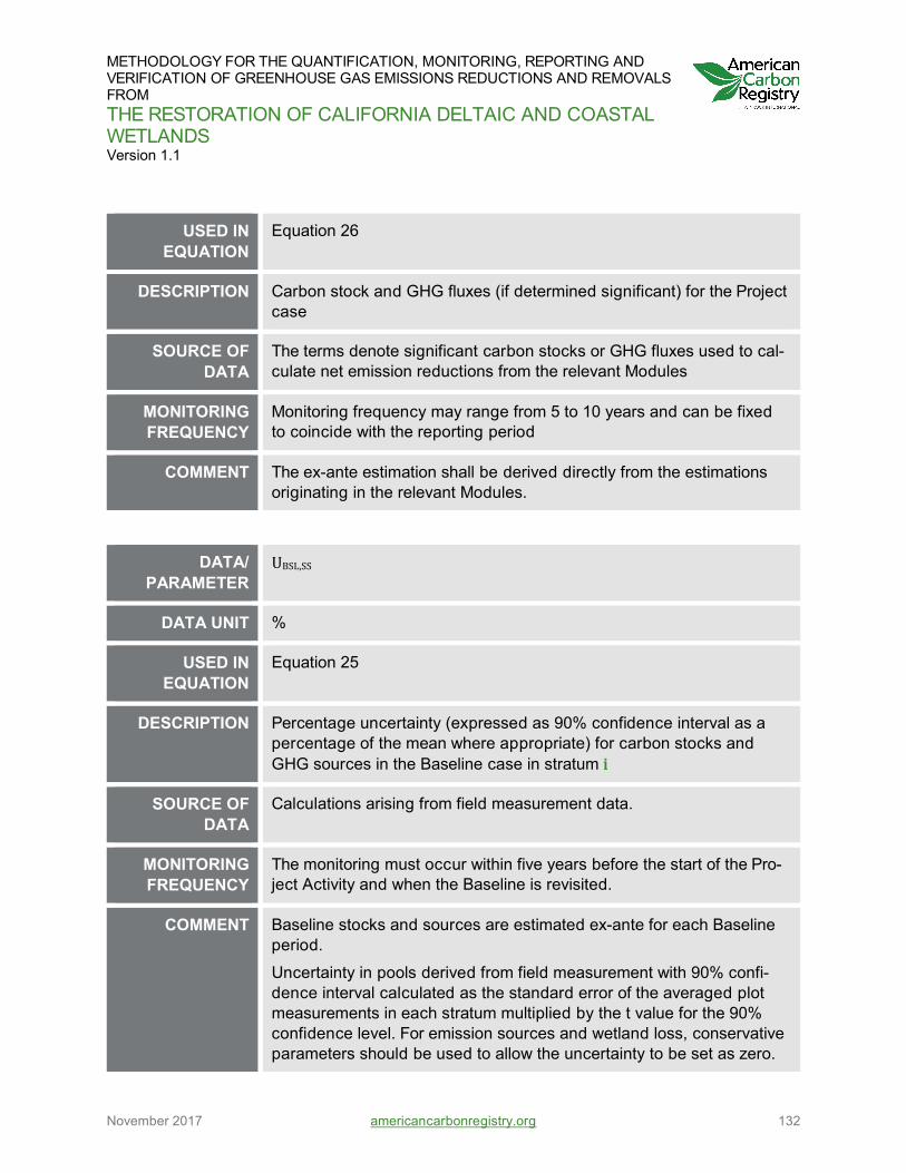
METHODOLOGY FOR THE QUANTIFICATION, MONITORING, REPORTING AND VERIFICATION OF GREENHOUSE GAS EMISSIONS REDUCTIONS AND REMOVALS FROM THE RESTORATION OF CALIFORNIA DELTAIC AND COASTAL WETLANDS Version 1.1
November 2017 americancarbonregistry.org 132
USED IN EQUATION
Equation 26
DESCRIPTION Carbon stock and GHG fluxes (if determined significant) for the Project case
SOURCE OF DATA
The terms denote significant carbon stocks or GHG fluxes used to cal-culate net emission reductions from the relevant Modules
MONITORING FREQUENCY
Monitoring frequency may range from 5 to 10 years and can be fixed to coincide with the reporting period
COMMENT The ex-ante estimation shall be derived directly from the estimations originating in the relevant Modules.
DATA/ PARAMETER
UBSL,SS
DATA UNIT %
USED IN EQUATION
Equation 25
DESCRIPTION Percentage uncertainty (expressed as 90% confidence interval as a percentage of the mean where appropriate) for carbon stocks and GHG sources in the Baseline case in stratum i
SOURCE OF DATA
Calculations arising from field measurement data.
MONITORING FREQUENCY
The monitoring must occur within five years before the start of the Pro-ject Activity and when the Baseline is revisited.
COMMENT Baseline stocks and sources are estimated ex-ante for each Baseline period.
Uncertainty in pools derived from field measurement with 90% confi-dence interval calculated as the standard error of the averaged plot measurements in each stratum multiplied by the t value for the 90% confidence level. For emission sources and wetland loss, conservative parameters should be used to allow the uncertainty to be set as zero.

METHODOLOGY FOR THE QUANTIFICATION, MONITORING, REPORTING AND VERIFICATION OF GREENHOUSE GAS EMISSIONS REDUCTIONS AND REMOVALS FROM THE RESTORATION OF CALIFORNIA DELTAIC AND COASTAL WETLANDS Version 1.1
November 2017 americancarbonregistry.org 133
DATA/ PARAMETER
UP,SS
DATA UNIT %
USED IN EQUATION
Equation 26
DESCRIPTION Percentage uncertainty (expressed as 90% confidence interval as a percentage of the mean where appropriate) for carbon stocks and GHG sources in the Project case
SOURCE OF DATA
Calculations arising from field measurement data
MONITORING FREQUENCY
Monitoring frequency may range from 5 to 10 years and can be fixed to coincide with the reporting period
COMMENT Uncertainty in pools derived from field measurement with 90% confi-dence interval calculated as the standard error of the averaged plot measurements in each stratum multiplied by the t value for the 90% confidence level. For emission sources and wetland loss conservative parameters should be used to allow the uncertainty to be set as zero.
4.5 (T-RISK) TOOL FOR ESTIMATING PERMANENCE AND RISK
The Project will employ the non-permanence risk tool currently approved by ACR as refer-enced in the ACR Standard.
4.6 (T-SIG) TOOL FOR SIGNIFICANCE TESTING The currently acceptable significance testing tool is the Clean Development Mechanism (CDM) tool for testing significance of GHG emissions, which can be found at:
http://cdm.unfccc.int/methodologies/ARmethodologies/tools/ar-am-tool-04-v1.pdf/history_view

METHODOLOGY FOR THE QUANTIFICATION, MONITORING, REPORTING AND VERIFICATION OF GREENHOUSE GAS EMISSIONS REDUCTIONS AND REMOVALS FROM THE RESTORATION OF CALIFORNIA DELTAIC AND COASTAL WETLANDS Version 1.1
November 2017 americancarbonregistry.org 134
4.7 (T-PLOT) TOOL FOR DESIGNING A FIELD SAMPLING PLAN FOR PLOTS
The currently acceptable tool is the Clean Development Mechanism (CDM) tool for calculation of the number of sample plots for measurements, which can be found at:
http://cdm.unfccc.int/methodologies/ARmethodologies/tools/ar-am-tool-03-v2.1.0.pdf/his-tory_view

METHODOLOGY FOR THE QUANTIFICATION, MONITORING, REPORTING AND VERIFICATION OF GREENHOUSE GAS EMISSIONS REDUCTIONS AND REMOVALS FROM THE RESTORATION OF CALIFORNIA DELTAIC AND COASTAL WETLANDS Version 1.1
November 2017 americancarbonregistry.org 135
DEFINITIONS If not explicitly defined here, the current definitions in the most recent version of the American Carbon Registry (ACR) Standard apply.
Baseline Most likely management scenario in the absence of the Project
Ex-ante “Before the event” or predicted response of Project activity
Ex-post “After the event” or measured response of Project activity
Historical Reference Period
The historical period prior to the Project start date that serves as the source of data for defining the Baseline
i Subscript used to represent a stratum
Leakage Leakage refers to a decrease in sequestration or increase in emissions outside project boundaries as a result of project implementation. Leakage may be caused by shifting of the activities of people present in the project area, or by market effects whereby emission reductions are countered by emissions created by shifts in supply of and demand for the products and services affected by the project.
Module Component of a methodology that can be applied on its own to perform a specific task
Offset Reduction in emissions of GHG made in order to compensate for or to offset an emission made elsewhere
Open Water Inundated coastal areas where there are areas of 10% or less emergent vegetation
Permanently Flooded Wetlands
Areas that are inundated during the entire year and in which there is wetland vegetation. Water levels range from land surface to 1 m above land surface.
Project Proponent
An individual or entity that undertakes, develops, and/or owns a project. This may include the project investor, designer, and/or owner of the lands/facilities on which project activities are conducted. The Project Proponent and

METHODOLOGY FOR THE QUANTIFICATION, MONITORING, REPORTING AND VERIFICATION OF GREENHOUSE GAS EMISSIONS REDUCTIONS AND REMOVALS FROM THE RESTORATION OF CALIFORNIA DELTAIC AND COASTAL WETLANDS Version 1.1
November 2017 americancarbonregistry.org 136
landowner/facility owner may be different entities. The Project Proponent is the ACR account holder.
Stratification A standard statistical procedure to decrease overall variability of carbon stock estimates by grouping data taken from environments with similar characteristics (e.g., vegetation type, age class, hydrology, elevation)
Seasonal Wetlands
Seasonally flooded areas containing wetland vegetation that are drained during at least 5 consecutive months during the spring and summer.
Tidal Wetlands
Wetlands affected by the cyclic changes in water levels caused by the tidal cycle. They are closely linked to estuaries where sea water mixes with fresh water to form an environment of varying salinities.
Tool Guideline or procedure for performing an analysis (e.g., tool for testing significance of GHG emissions in A/R CDM Project activities) or to help use or select a module or methodology.

METHODOLOGY FOR THE QUANTIFICATION, MONITORING, REPORTING AND VERIFICATION OF GREENHOUSE GAS EMISSIONS REDUCTIONS AND REMOVALS FROM THE RESTORATION OF CALIFORNIA DELTAIC AND COASTAL WETLANDS Version 1.1
November 2017 americancarbonregistry.org 137
Leakage is an increase in the global warming potential (GWP) (i.e., changes in greenhouse emissions [GHG] or removals) outside the Project boundaries that occurs because of the Pro-ject action. The American Carbon Registry (ACR) requires Project Proponents to assess, ac-count for, and mitigate for leakage above de-minimis levels. Project Proponents must deduct leakage that reduces the GWP benefit of a Project in excess of the applicable threshold speci-fied in the methodology.
Activity-shifting leakage occurs when the land uses resulting in baseline emissions that oper-ated in the Project area before the Project start date are relocated to another area outside of the Project boundary. Such market-effects leakage is transmitted through market forces: a sup-ply reduction can result in an upward pressure on price that may incentivize increased produc-tion and shifts in cropping patterns elsewhere. The change in the GWP as the result of these market-effects leakage shall be accounted for in the net Project GHG removals. For the activi-ties included in this methodology, the market-effects leakage would result from replacement of crops currently grown in the Sacramento-San Joaquin Delta (Delta) by wetlands and rice.
An analysis is presented of leakage for replacement of traditional crops in the Delta with wet-lands and rice. First, an economic analysis was conducted to determine how crop acreages statewide would be affected by Delta land conversion. Next we estimated the change in GWP as the result of this crop-area change.

METHODOLOGY FOR THE QUANTIFICATION, MONITORING, REPORTING AND VERIFICATION OF GREENHOUSE GAS EMISSIONS REDUCTIONS AND REMOVALS FROM THE RESTORATION OF CALIFORNIA DELTAIC AND COASTAL WETLANDS Version 1.1
November 2017 americancarbonregistry.org 138
ERA Economics (see ERA technical memorandum below) used the Statewide Agricultural Pro-duction (SWAP) model10 to quantify market leakage. The purpose of this analysis was to evalu-ate the potential “leakage” effects for four Delta land-use-change scenarios. For the purposes of this analysis, market leakage is defined as the shift in agricultural production to other regions of California as a result of land changes in the Delta. Land use change from traditional crops to wetlands and rice in the model has been imposed as an exogenous policy constraint in the model.
The SWAP model is a regional agricultural production and economic optimization model that simulates decisions by farmers across 93 percent of agricultural land in California (over 6 mil-lion acres). It is the most current in a series of California agricultural production models origi-nally developed by researchers at the University of California at Davis in collaboration with the California Department of Water Resources. The SWAP model and its predecessor, the Central Valley Production Model (CVPM), have been used for numerous policy analyses and impact studies over the past 15 years, including the economic implications of Delta conveyance op-tions11 and has been subject to peer review.
For this analysis, the 27 Central Valley SWAP model regions were aggregated into 4 regions: Sacramento Valley, Delta, San Joaquin River, and Tulare Lake Basin. Additional SWAP model regions along the central coast and southern California were not included in the analysis be-cause these regions are decoupled from the Central Valley market. The 20 standard crop groups modeled in SWAP were aggregated into 7 groups: trees and vineyards; irrigated pas-ture; rice; miscellaneous field crops including corn; forage and other field crops; vegetables; and cotton.
The SWAP model was used to estimate crop acreage changes for the following alternatives in which land-use changes were simulated to occur by 2030: conversion of traditional field crops and pasture to wetlands or rice. There is no option for implementing wetlands in the SWAP model so it was assumed that fallow land would adequately represent wetlands. Field crops and pasture predominate in areas where there are oxidizing organic soils that contribute to baseline carbon dioxide emissions.
10 R. E. Howitt, J. Medellin-Azuara, D. MacEwan, and J. R. Lund. (2012). Calibrating disaggregate eco-
nomic models of agricultural production and water management. Environmental Modeling and Soft-ware 38, 244-258.
11 D. MacEwan and S. Hatchett. (2012). Statewide Agricultural Production Model Update and Application to Federal Feasibility Analysis. Prepared for United States Department of the Interior, Bureau of Recla-mation Mid-Pacific Region. 104 pp.
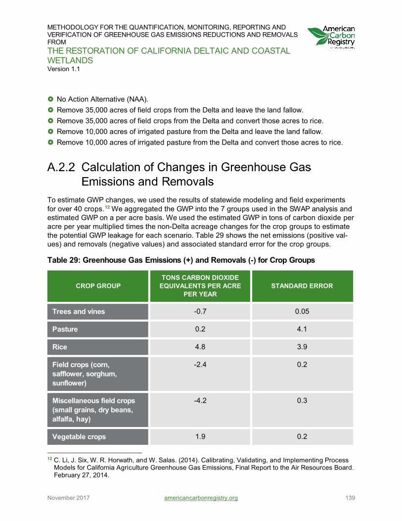
METHODOLOGY FOR THE QUANTIFICATION, MONITORING, REPORTING AND VERIFICATION OF GREENHOUSE GAS EMISSIONS REDUCTIONS AND REMOVALS FROM THE RESTORATION OF CALIFORNIA DELTAIC AND COASTAL WETLANDS Version 1.1
November 2017 americancarbonregistry.org 139
No Action Alternative (NAA). Remove 35,000 acres of field crops from the Delta and leave the land fallow. Remove 35,000 acres of field crops from the Delta and convert those acres to rice. Remove 10,000 acres of irrigated pasture from the Delta and leave the land fallow. Remove 10,000 acres of irrigated pasture from the Delta and convert those acres to rice.
To estimate GWP changes, we used the results of statewide modeling and field experiments for over 40 crops.12 We aggregated the GWP into the 7 groups used in the SWAP analysis and estimated GWP on a per acre basis. We used the estimated GWP in tons of carbon dioxide per acre per year multiplied times the non-Delta acreage changes for the crop groups to estimate the potential GWP leakage for each scenario. Table 29 shows the net emissions (positive val-ues) and removals (negative values) and associated standard error for the crop groups.
Table 29: Greenhouse Gas Emissions (+) and Removals (-) for Crop Groups
CROP GROUP TONS CARBON DIOXIDE
EQUIVALENTS PER ACRE PER YEAR
STANDARD ERROR
Trees and vines -0.7 0.05
Pasture 0.2 4.1
Rice 4.8 3.9
Field crops (corn, safflower, sorghum, sunflower)
-2.4 0.2
Miscellaneous field crops (small grains, dry beans, alfalfa, hay)
-4.2 0.3
Vegetable crops 1.9 0.2
12 C. Li, J. Six, W. R. Horwath, and W. Salas. (2014). Calibrating, Validating, and Implementing Process
Models for California Agriculture Greenhouse Gas Emissions, Final Report to the Air Resources Board. February 27, 2014.
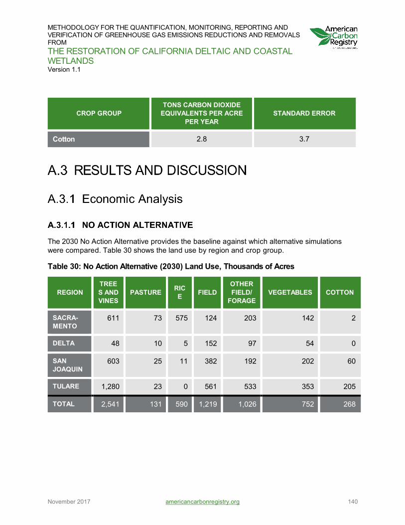
METHODOLOGY FOR THE QUANTIFICATION, MONITORING, REPORTING AND VERIFICATION OF GREENHOUSE GAS EMISSIONS REDUCTIONS AND REMOVALS FROM THE RESTORATION OF CALIFORNIA DELTAIC AND COASTAL WETLANDS Version 1.1
November 2017 americancarbonregistry.org 140
CROP GROUP TONS CARBON DIOXIDE
EQUIVALENTS PER ACRE PER YEAR
STANDARD ERROR
Cotton 2.8 3.7
The 2030 No Action Alternative provides the baseline against which alternative simulations were compared. Table 30 shows the land use by region and crop group.
Table 30: No Action Alternative (2030) Land Use, Thousands of Acres
REGION TREES AND VINES
PASTURE RICE FIELD
OTHER FIELD/
FORAGE VEGETABLES COTTON
SACRA-MENTO
611 73 575 124 203 142 2
DELTA 48 10 5 152 97 54 0
SAN JOAQUIN
603 25 11 382 192 202 60
TULARE 1,280 23 0 561 533 353 205
TOTAL 2,541 131 590 1,219 1,026 752 268

METHODOLOGY FOR THE QUANTIFICATION, MONITORING, REPORTING AND VERIFICATION OF GREENHOUSE GAS EMISSIONS REDUCTIONS AND REMOVALS FROM THE RESTORATION OF CALIFORNIA DELTAIC AND COASTAL WETLANDS Version 1.1
November 2017 americancarbonregistry.org 141
The predominant crops in the Central Delta where wetlands and rice would likely be imple-mented to mitigate subsidence and provide a greenhouse removal benefit are field crops (pri-marily corn) and pasture. Thus, the alternative simulations replaced these crops with wetlands and rice. Table 32 shows the statewide acreage changes for the alternatives.
RETIRE 35,000 ACRES FIELD CROPS AND CONVERT TO WETLANDS
In alternative 2, 35,000 acres of field crops (corn, safflower, and “other field crops”) are con-verted to wetlands. The statewide change in the total agricultural footprint is slightly less than 35,000 acres, indicating limited crop substitution to other regions as farmers adjust crop mix in response to changing relative prices. Most of the acreage change occurs in the Delta.
RETIRE 35,000 ACRES FIELD CROPS AND CONVERT TO RICE
Alternative 3 is the same as alternative 2 except the 35,000 acres are converted entirely to rice. The estimated statewide decrease in the total agricultural footprint is estimated to be less than 20,000 acres. There is a simulated decrease in rice acreage in the Sacramento Valley, the pri-mary rice-producing area in the state.
RETIRE 10,000 ACRES IRRIGATED PASTURE AND CONVERT TO WETLANDS
In alternative 4, 10,000 acres of pasture are removed from the Delta and that land is converted to wetlands. Statewide, net acreage changed by approximately the same amount.
RETIRE 10,000 ACRES IRRIGATED PASTURE AND CONVERT TO RICE
Alternative 5 is the same as alternative 4 except the pasture acreage is converted entirely to rice. The estimated statewide change in the total agricultural footprint is estimated to be less than 1,000 acres. The primary land use change would occur in the Delta where rice replaces pasture. Some acreage is simulated to go out of rice production in the Sacramento Valley.

METHODOLOGY FOR THE QUANTIFICATION, MONITORING, REPORTING AND VERIFICATION OF GREENHOUSE GAS EMISSIONS REDUCTIONS AND REMOVALS FROM THE RESTORATION OF CALIFORNIA DELTAIC AND COASTAL WETLANDS Version 1.1
November 2017 americancarbonregistry.org 142
Table 31: Acreage Changes by Region and Crop Group for Alternatives Relative to the NAA
SCENARIO REGION TREES
AND VINES
PAS-TURE RICE FIELD
OTHER FIELD/
FORAGE VEGE-
TABLES COT-TON
A2 FIELD CROPS TO WET-LANDS
SACRA-MENTO -9 -178 -5 920 -247 -49 -1
DELTA -522 5,119 6 -35,992 -2,948 -662 0
SAN JOAQUIN -106 -72 -2 853 -359 -51 -45
TULARE -101 -498 0 1,422 -384 -36 -96
A2 TOTAL NET CHANGE
-34,043 -738 4371 -1 -32,797 -3,938 -798 -142
A3 FIELD CROPS TO RICE
SACRA-MENTO 2,414 557 -2,919 914 583 124 55
DELTA -257 -10,071 35,000 -35,000 -11,029 -449 0
SAN JOAQUIN -447 -59 -111 630 133 -53 -49
TULARE -276 -364 0 664 172 -66 -201
A3 TOTAL NET CHANGE
-20,105 1,434 -9,937 31,970 -32,792 -10,141 -444 -195
A4 PASTURE TO WET-LANDS
SACRA-MENTO -11 110 11 14 -77 -2 0
DELTA -54 -10,000 71 -1,768 1,732 19 0
SAN JOAQUIN 31 60 3 79 -118 -1 1
TULARE 24 114 0 62 -148 10 42

METHODOLOGY FOR THE QUANTIFICATION, MONITORING, REPORTING AND VERIFICATION OF GREENHOUSE GAS EMISSIONS REDUCTIONS AND REMOVALS FROM THE RESTORATION OF CALIFORNIA DELTAIC AND COASTAL WETLANDS Version 1.1
November 2017 americancarbonregistry.org 143
SCENARIO REGION TREES
AND VINES
PAS-TURE RICE FIELD
OTHER FIELD/
FORAGE VEGE-
TABLES COT-TON
TOTAL NET CHANGE
-9,796 -10 -9,716 85 -1,613 1,389 26 43
A5 PAS-TURE TO RICE
SACRA-MENTO 883 298 -936 -11 186 56 18
DELTA 4 -10,000 10,000 60 378 11 0
SAN JOAQUIN -73 48 -26 52 12 1 -1
TULARE -33 78 0 -23 1 2 3
TOTAL NET CHANGE
988 781 -9,576 9,038 78 577 70 20
RETIRE 35,000 ACRES OF FIELD CROPS AND CONVERT TO WETLANDS
We estimated the GHG effect of changes in crop acreage outside the Delta on the GWP (Table 33). Due to simulated changes in price, supply, and demand, the SWAP model estimated a to-tal change of 5,431 acres for the non-Delta region. For each crop group, the change in acre-age was multiplied by the emissions or removals listed in Table 30 to result in a net removal of 4,198 tons carbon dioxide equivalents per year relative to the NAA (Table 33). For comparison, estimated median baseline emissions in the Delta are about 7 tons carbon dioxide equivalents per acre per year13 due to the oxidation of organic soils. Therefore, for the 35,000 acres of field crops in the Delta, the estimated baseline emission is about 245,000 tons carbon dioxide equivalents per year. The estimated standard error associated with the GWP is relatively large
13 S. J. Deverel and D. A. Leighton. (2010). Historic, recent, and future subsidence, Sacramento-San
Joaquin Delta, California, USA. San Francisco Estuary and Watershed Science 8(2). http://www.escholarship.org/uc/item/7xd4x0xw.

METHODOLOGY FOR THE QUANTIFICATION, MONITORING, REPORTING AND VERIFICATION OF GREENHOUSE GAS EMISSIONS REDUCTIONS AND REMOVALS FROM THE RESTORATION OF CALIFORNIA DELTAIC AND COASTAL WETLANDS Version 1.1
November 2017 americancarbonregistry.org 144
as there is substantial variability within crop groups and spatial and temporal variability associ-ated with the modeled and measured values. Considering the total standard error (the sum of absolute values for individual crop groups) results in a range of GWP change relative to the NAA of -8,790 to 395 tons carbon dioxide equivalents per year.
Table 32: Change in Acreage and Greenhouse Gas Emissions Due to Conversion to Wetlands in Alternative 2
TREES
AND VINES
PAS-TURE RICE FIELD
OTHER FIELD/
FORAGE
VEGETA-BLES
COT-TON TOTAL
Non-Delta acreage change
-215 -748 -7 3,195 -990 -135 -141 5,431
Non-Delta GWP change (tons carbon dioxide equivalents per year)
151 -150 -35 -7,667 4,156 -257 -396 -4,198
Estimated GWP Stand-ard Error
11 3,067 29 639 297 27 524 4,593
RETIRE 35,000 ACRES OF FIELD CROPS AND CONVERT TO RICE
For this alternative, the SWAP model estimated a total non-Delta acreage change of 8,152 acres (Table 34). For each crop group, the change in acreage was multiplied by the emissions or re-movals listed in Table 30 to result in a net GWP change of -25,270 tons carbon dioxide equiva-lents per year relative to the NAA. A key reason for the large net removal is the decrease in non-Delta rice acreage, which was multiplied by the estimated per acre emissions of 4.8 tons car-bon dioxide equivalents per acre per year on mineral soils in California (Table 30). Similar to Al-ternative 2 and for comparison, the estimated baseline emission for the 35,000 acres of field crops in the Delta is about 245,000 tons carbon dioxide equivalents per year. Considering the total standard error (the sum of absolute values for individual crop groups) results in a range of GWP change relative to the NAA of -39,156 to -11,383 tons carbon dioxide equivalents per year.

METHODOLOGY FOR THE QUANTIFICATION, MONITORING, REPORTING AND VERIFICATION OF GREENHOUSE GAS EMISSIONS REDUCTIONS AND REMOVALS FROM THE RESTORATION OF CALIFORNIA DELTAIC AND COASTAL WETLANDS Version 1.1
November 2017 americancarbonregistry.org 145
Table 33: Change in Acreage and GWP Due to Conversion to Rice in Alternative 3
TREES
AND VINES
PAS-TURE RICE FIELD
OTHER FIELD/
FORAGE
VEGE-TABLES
COT-TON TOTAL
Non-Delta acreage change
1,691 134 -3,031 2,208 888 5 -195 8,152
Non-Delta GWP change (tons car-bon diox-ide equiv-alents)
-1,183 27 -14,547 -5,299 -3,730 10 -547 -25,270
Estimated GWP Standard Error
85 551 11,819 442 266 1 723 13,886
RETIRE 10,000 ACRES OF PASTURE AND CONVERT TO WETLANDS
For this alternative, the SWAP model estimated a total non-Delta acreage change of 1,269 acres. For each crop group, the change in acreage was multiplied by the emissions or remov-als listed in Table 30 to result in a net GWP change of 1,296 tons carbon dioxide equivalents per year relative to the NAA (Table 35). For comparison, estimated median baseline emissions in the Delta are about 7 tons carbon dioxide equivalents per acre per year. Therefore, for the 10,000 acres of pasture in the Delta, the estimated baseline emission is about 70,000 tons car-bon dioxide equivalents per year. The estimated change in the GWP is less than 2% of the esti-mated baseline emission. Considering the total standard error (the sum of absolute values for individual crop groups), results in a range of GWP change relative to the NAA of -221 to 2,813 tons carbon dioxide equivalents per year or a maximum of 4% of baseline emissions.

METHODOLOGY FOR THE QUANTIFICATION, MONITORING, REPORTING AND VERIFICATION OF GREENHOUSE GAS EMISSIONS REDUCTIONS AND REMOVALS FROM THE RESTORATION OF CALIFORNIA DELTAIC AND COASTAL WETLANDS Version 1.1
November 2017 americancarbonregistry.org 146
Table 34: Change in Acreage and Annual Greenhouse Gas Emissions Due to Conversion to Wetlands in Alternative 4
TREES
AND VINES
PAS-TURE RICE FIELD
OTHER FIELD/
FORAGE
VEGE-TABLES
COT-TON TOTAL
Non-Delta acreage change
43 284 14 155 -343 6 43 890
Non-Delta GWP change (tons car-bon diox-ide equiv-alents)
-30 57 69 -373 1,441 12 121 1,296
Estimated GWP Standard Error
2 1,164 56 31 103 1 160 1,517
RETIRE 10,000 ACRES OF PASTURE AND CONVERT TO RICE
For this alternative, the SWAP model estimated a total non-Delta acreage change of 2,460 acres. For each crop group, the change in acreage was multiplied by the emissions or remov-als listed in Table 30 to result in a net GWP change of -5,788 tons carbon dioxide equivalents per year relative to the NAA. The decrease in rice acreage outside the Delta represents the majority of the change in the GWP. Similar to Alternative 4 and for comparison, the estimated baseline emission for the 10,000 acres of pasture in the Delta is about 70,000 tons carbon di-oxide equivalents per year. Considering the total standard error (the sum of absolute values for individual crop groups) results in a range of GWP change relative to the NAA of -11,465 to -111 tons carbon dioxide equivalents per year.

METHODOLOGY FOR THE QUANTIFICATION, MONITORING, REPORTING AND VERIFICATION OF GREENHOUSE GAS EMISSIONS REDUCTIONS AND REMOVALS FROM THE RESTORATION OF CALIFORNIA DELTAIC AND COASTAL WETLANDS Version 1.1
November 2017 americancarbonregistry.org 147
Table 35: Change in Acreage and Annual Greenhouse Gas Emissions Due to Conversion to Wetlands in Alternative 5
TREES
AND VINES
PAS-TURE RICE FIELD
OTHER FIELD/
FORAGE
VEGE-TABLES
COT-TON TOTAL
Non-Delta acreage change
777 424 -962 18 199 60 20 2,460
Non-Delta GWP change (tons car-bon diox-ide equiv-alents)
-544 85 -4,619 -44 -835 114 55 -5,788
Estimated GWP Standard Error
39 1,737 3,753 4 60 12 73 5,677
Holistic economic and GWP analysis of likely land use changes in California due to implemen-tation of rice and wetlands in the Delta provides useful and insightful information about poten-tial market-based leakage. For four alternatives in which we simulated the changes in agricul-tural acreages resultant from conversion of traditional crops to wetlands and rice in the Delta, estimated GWP changes were insignificant relative to the no-action alternative and baseline emissions or there was a net GWP benefit. The following bullets summarize our results:
Retirement of 35,000 acres of field crops and conversion to wetlands resulted in a non-Delta GWP change of -4,198 tons carbon dioxide equivalents per year. The baseline emissions associated with field crops is about 245,000 tons carbon dioxide equivalents per year.
Retirement of 35,000 acres of field crops and conversion to rice resulted in a non-Delta GWP change of -25,270 tons carbon dioxide equivalents per year. The baseline emissions associated with field crops is about 245,000 tons carbon dioxide equivalents per year. A key reason for the large net removal is the decrease in non-Delta rice acreage that was then

METHODOLOGY FOR THE QUANTIFICATION, MONITORING, REPORTING AND VERIFICATION OF GREENHOUSE GAS EMISSIONS REDUCTIONS AND REMOVALS FROM THE RESTORATION OF CALIFORNIA DELTAIC AND COASTAL WETLANDS Version 1.1
November 2017 americancarbonregistry.org 148
multiplied by the estimated per acre emissions of 4.8 tons carbon dioxide equivalents per acre per year on mineral soils in California.
Retirement of 10,000 acres of pasture and conversion to wetlands resulted in a non-Delta GWP change of 1,296 tons carbon dioxide equivalents per year. The baseline emissions associated with pasture is about 70,000 tons carbon dioxide equivalents per year.
Retirement of 10,000 acres of pasture and conversion to rice result in a net GWP change of -5,788 tons carbon dioxide equivalents per year relative to the NAA. For comparison, the estimated baseline emission for the 10,000 acres of pasture in the Delta is about 70,000 tons carbon dioxide equivalents per year.
We estimated uncertainty by using the standard error associated with the GWP estimates. In all alternatives except for alternative 4, the range of GWP changes was insignificant (3% or less) relative to baseline emissions.
Where rice acreage increases in the Delta, our results indicate a net statewide GWP benefit due to the decrease in rice acreage in non-Delta areas where there are large GHG emissions on mineral soils.
Prepared by: Duncan MacEwan, ERA Economics Prepared for: Steve Deverel, HydroFocus August 12, 2014
This technical memorandum briefly describes the methods, results, and limitations of an eco-nomic analysis of land use change in the Sacramento-San Joaquin Delta (Delta) using the Statewide Agricultural Production (SWAP) model. The purpose of this analysis was to evaluate the potential “leakage” effects from four (4) Delta land use policies. Leakage is a term used to describe the offset of carbon (or other) policy benefits caused by a shift in economic activity to another region. For the purposes of this analysis, leakage is defined as the shift in agricultural production to other regions of California as a result of land retirement policies in the Delta.
It is important to note that changes in land use resulting from environmental (e.g., carbon) pol-icy, and the partial offsetting effects of leakage, are clearly driven by the economics of the crops being produced. An effective Delta land use policy must alter the relative profitability of crops, considering conditions in domestic and international export markets, in order to incen-tivize growers to shift production systems or retire land. In this analysis no attempt has been made to model land use change as an endogenous outcome of some incentive structure. In-stead, land use change has been imposed as an exogenous policy constraint. It follows that this study should be viewed as a partial equilibrium analysis of Delta land use policy that is mandated and therefore decoupled entirely from economics, holding all other factors constant. The estimated leakage represents one outcome resulting from a series of critically important

METHODOLOGY FOR THE QUANTIFICATION, MONITORING, REPORTING AND VERIFICATION OF GREENHOUSE GAS EMISSIONS REDUCTIONS AND REMOVALS FROM THE RESTORATION OF CALIFORNIA DELTAIC AND COASTAL WETLANDS Version 1.1
November 2017 americancarbonregistry.org 149
simplifying assumptions. In practice, a significant incentive structure would need to be in place to affect the type and scale of land use conversion considered in this analysis.
More careful general equilibrium and sensitivity analysis should be performed prior to drawing any policy conclusions from the results summarized in this technical memorandum.
The SWAP model is a regional agricultural production and economic optimization model that simulates the decisions of farmers across 93 percent of agricultural land in California. It is the most current in a series of California agricultural production models, originally developed by researchers at the University of California at Davis in collaboration with the California Depart-ment of Water Resources with additional funding provided by the United States Bureau of Rec-lamation. The SWAP model has been subject to peer-review (Howitt et al. 2012). The SWAP model and its predecessor the Central Valley Production Model (CVPM) have been used for numerous policy analyses and impact studies over the past 15 years, including the impacts of the Central Valley Project Improvement Act, Upper San Joaquin Basin Storage Investigation, the SWP drought impact analysis, and the economic implications of Delta conveyance options (MacEwan and Hatchett 2012).
The SWAP model was used to estimate the following scenarios (alternatives):
No Action Alternative (NAA) Remove 35,000 acres of field crops from the Delta and leave the land fallow Remove 35,000 acres of field crops from the Delta and convert those acres to rice Remove 10,000 acres of irrigated pasture from the Delta and leave the land fallow Remove 10,000 acres of irrigated pasture from the Delta and convert those acres to rice
Field crops for this analysis were defined as safflower, sudan grass and other miscellaneous field crops, and corn. Year 2030 was assumed for the level of development. Other key as-sumptions include:
Crop demand: linear shift based on changes in real income and population. No attempt was made to model international export markets, it was assumed that California maintains a constant export share in the international market.
Real electricity cost: held constant. Other inputs real cost: held constant. Technological change: not modeled. Climate effects (changes in crop yield and ET): not modeled.

METHODOLOGY FOR THE QUANTIFICATION, MONITORING, REPORTING AND VERIFICATION OF GREENHOUSE GAS EMISSIONS REDUCTIONS AND REMOVALS FROM THE RESTORATION OF CALIFORNIA DELTAIC AND COASTAL WETLANDS Version 1.1
November 2017 americancarbonregistry.org 150
Surface water deliveries: CVP, SWP, and local supplies were held constant. Groundwater depth and installed capacity: held constant. Urban development (ag-urban land conversion): not modeled.
The impact of an alternative is defined as the difference between the NAA and that alternative. This analysis holds all other factors constant, given the assumptions described above, to esti-mate the shift in statewide crop production in response to each policy alternative.
The 27 Central Valley SWAP model regions were aggregated into 4 regions, including the Sac-ramento Valley, Delta, San Joaquin River, and Tulare Lake Basin. Additional SWAP model re-gions along the central coast and southern California were not included in the analysis be-cause these regions are generally decoupled from the Central Valley market. The 20 standard crop groups modeled in SWAP were aggregated into 7 groups: trees and vineyards, irrigated pasture, rice, miscellaneous field crops including corn, forage and other field crops, vegeta-bles, and cotton. The accompanying Excel workbook summarizes the results. This section pro-vides a brief summary of the findings.
The 2030 NAA provides the baseline against which the future policy runs are compared. Agri-cultural land use is expected to contract slightly by 2030, by around 6.5 million irrigated acres (~5%) statewide, including a contraction to 367,000 acres in the Delta. This is consistent with the recent trends in California toward more intensive tree and specialty crop production on a smaller land footprint. Climate change, international markets, relative energy costs, and re-source conditions such as surface and groundwater availability will affect the 2030 NAA, but were held constant in this analysis. Irrigated pasture in the Delta is estimated to decrease from approximately 14,000 acres to 10,000 acres.
Table 36: No Action Alternative (2030) Land Use, Thousands of Acres
REGION TREES
AND VINES
PASTURE RICE FIELD OTHER FIELD/
FORAGE VEGETABLES COTTON
SACRA-MENTO 611 73 575 124 203 142 2
DELTA 48 10 5 152 97 54 0

METHODOLOGY FOR THE QUANTIFICATION, MONITORING, REPORTING AND VERIFICATION OF GREENHOUSE GAS EMISSIONS REDUCTIONS AND REMOVALS FROM THE RESTORATION OF CALIFORNIA DELTAIC AND COASTAL WETLANDS Version 1.1
November 2017 americancarbonregistry.org 151
REGION TREES
AND VINES
PASTURE RICE FIELD OTHER FIELD/
FORAGE VEGETABLES COTTON
SAN JOAQUIN 603 25 11 382 192 202 60
TULARE 1,280 23 0 561 533 353 205
ALTERNATIVE 2 – RETIRE 35,000 ACRES FIELD CROPS
In alternative 2, 35,000 acres of field crops (corn, safflower, and “other field crops”) are re-moved from the Delta and the land is left fallow. The statewide change in the total irrigated footprint is slightly less than 35,000 acres, indicating limited crop substitution to other regions as farmers adjust crop mix in response to changing relative prices.
Table 37: Alternative 2 (2030) Land Use, Thousands of Acres
REGION TREES AND VINES
PASTURE RICE FIELD
OTHER FIELD/
FORAGE VEGETABLES COTTON
SACRA-MENTO 611 73 575 125 203 142 2
DELTA 47 15 5 116 94 54 0
SAN JOAQUIN 603 25 11 383 192 202 60
TULARE 1,280 23 0 563 533 353 205
ALTERNATIVE 3 – RETIRE 35,000 ACRES FIELD CROPS AND CONVERT TO RICE
Alternative 3 is the same as alternative 2 except the acreage is converted entirely to rice. This analysis assumed that land use conversion is exogenously mandated. The statewide decrease in the total irrigated footprint is estimated to be less than 20,000 acres.

METHODOLOGY FOR THE QUANTIFICATION, MONITORING, REPORTING AND VERIFICATION OF GREENHOUSE GAS EMISSIONS REDUCTIONS AND REMOVALS FROM THE RESTORATION OF CALIFORNIA DELTAIC AND COASTAL WETLANDS Version 1.1
November 2017 americancarbonregistry.org 152
Table 38: Alternative 3 (2030) Land Use, Thousands of Acres
REGION TREES AND VINES
PASTURE RICE FIELD
OTHER FIELD/
FORAGE VEGETABLES COTTON
SACRA-MENTO 613 73 572 125 204 143 3
DELTA 48 0 40 117 86 54 0
SAN JOAQUIN 603 25 10 383 192 202 60
TULARE 1,280 23 0 562 534 353 205
ALTERNATIVE 4 – RETIRE 10,000 ACRES IRRIGATED PASTURE
In alternative 4, 10,000 acres of irrigated pasture are removed from the Delta and that land is left fallow. Statewide irrigated acreage decreases by approximately the same amount.
Table 39: Alternative 4 (2030) Land Use, Thousands of Acres
REGION TREES AND VINES
PASTURE RICE FIELD
OTHER FIELD/
FORAGE VEGETABLES COTTON
SACRA-MENTO 611 73 575 124 203 142 2
DELTA 48 0 5 150 99 54 0
SAN JOAQUIN 603 25 11 382 192 202 60
TULARE 1,280 23 0 561 533 353 205
ALTERNATIVE 5 – RETIRE 13,800 ACRES IRRIGATED PASTURE AND CONVERT TO RICE
Alternative 5 is the same as alternative 4 except the acreage is converted entirely to rice. It is important to note, again, that this analysis assumed that land use conversion is exogenously mandated. The statewide total irrigated area is estimated to increase by just over 1,000 acres.

METHODOLOGY FOR THE QUANTIFICATION, MONITORING, REPORTING AND VERIFICATION OF GREENHOUSE GAS EMISSIONS REDUCTIONS AND REMOVALS FROM THE RESTORATION OF CALIFORNIA DELTAIC AND COASTAL WETLANDS Version 1.1
November 2017 americancarbonregistry.org 153
Table 40: Alternative 5 (2030) Land Use, Thousands of Acres
REGION TREES AND VINES
PASTURE RICE FIELD
OTHER FIELD/
FORAGE VEGETABLES COTTON
SACRA-MENTO 611 73 574 124 204 143 3
DELTA 48 0 15 152 98 54 0
SAN JOAQUIN 603 25 11 382 192 202 60
TULARE 1,280 23 0 561 533 353 205
The leakage analysis is primarily concerned with the change in crop mix and shift in production to other regions of California. The leakage effect is fundamentally driven by basic supply and demand principles of economics. When the production of a crop(s) decreases in response to Delta land use policy, all else constant, the price of that crop(s) will increase. As the price of that crop(s) increases this will change the relative profitability of crops in all other regions in the state, and in response, growers may switch production systems and change the statewide crop mix. The magnitude of this effect is driven by a number of factors including domestic and international market conditions, the relative supply and demand elasticities of all crops, and cross-price elasticities. In addition, there are intensive margin (for example, input use per acre) adjustments to production that affect the magnitude of leakage. The following subsections briefly describe the results of the leakage analysis and summarize key trends.
ALTERNATIVE 2
A total of 35,992 acres of corn, other field, and safflower crops (35,000 attributed to the policy and 992 attributed to market adjustment) are removed from the Delta. 35,000 acres of land is left fallow and the total irrigated acreage in the Delta decreases by the same amount.
The decrease in Delta field crop production increases the statewide price for field crops, caus-ing an additional 3,200 acres to be planted in the Sacramento, San Joaquin and Tulare Basin areas of the Central Valley. The additional acreage in other regions comes from a small shift in the crop mix, meaning a decrease in the acreage of some other crops. For example, growers in the Tulare Lake Basin plant 500 fewer acres of irrigated pasture and substitute toward other field crops.

METHODOLOGY FOR THE QUANTIFICATION, MONITORING, REPORTING AND VERIFICATION OF GREENHOUSE GAS EMISSIONS REDUCTIONS AND REMOVALS FROM THE RESTORATION OF CALIFORNIA DELTAIC AND COASTAL WETLANDS Version 1.1
November 2017 americancarbonregistry.org 154
ALTERNATIVE 3
35,000 acres of field crops removed from the Delta are converted to rice. The increased rice production in the Delta puts downward pressure on rice prices and rice production decreases, primarily in the Sacramento Valley. In response to the decreased rice production, the Sacra-mento Valley production shifts to other crops including deciduous and forage crops. This causes a change in the market price of those crops and production decreases in other regions and the market reaches a new equilibrium.
ALTERNATIVE 4
A total of 10,000 acres of irrigated pasture are removed from the Delta and the land is left fal-low. Fallowing 10,000 acres of pasture has a small statewide price effect and other regions slightly increase production. There is a correspondingly small shift in the crop mix to accom-modate the increase in pasture acreage in these regions.
ALTERNATIVE 5
10,000 acres of irrigated pasture are removed from the Delta and converted to rice.
Similar to alternative 3, the increased rice production in the Delta puts downward pressure on rice prices and rice production decreases, primarily in the Sacramento Valley. The Sacramento Valley production adjusts and shifts to other crops including deciduous, pasture and other for-age crops. This causes a change in the market price of those crops and production adjusts in other regions until the market reaches a new equilibrium.
Table 41: Change in Irrigated Acreage from NAA
SCENARIO REGION TREES
AND VINES
PAS-TURE RICE FIELD
OTHER FIELD/
FORAGE VEGE-
TABLES COT-TON
A2 FALLOW FIELD
SACRA-MENTO -9 -178 -5 920 -247 -49 -1
DELTA -522 5,119 6 -35,992 -2,948 -662 0
SAN JOAQUIN -106 -72 -2 853 -359 -51 -45
TULARE -101 -498 0 1,422 -384 -36 -96
A3 FIELD TO RICE
SACRA-MENTO 2,414 557 -2,919 914 583 124 55
DELTA -257 -10,071 35,000 -35,000 -11,029 -449 0

METHODOLOGY FOR THE QUANTIFICATION, MONITORING, REPORTING AND VERIFICATION OF GREENHOUSE GAS EMISSIONS REDUCTIONS AND REMOVALS FROM THE RESTORATION OF CALIFORNIA DELTAIC AND COASTAL WETLANDS Version 1.1
November 2017 americancarbonregistry.org 155
SCENARIO REGION TREES
AND VINES
PAS-TURE RICE FIELD
OTHER FIELD/
FORAGE VEGE-
TABLES COT-TON
SAN JOAQUIN -447 -59 -111 630 133 -53 -49
TULARE -276 -364 0 664 172 -66 -201
A4 FALLOW PASTURE
SACRA-MENTO -11 110 11 14 -77 -2 0
DELTA -54 -10,000 71 -1,768 1,732 19 0
SAN JOAQUIN 31 60 3 79 -118 -1 1
TULARE 24 114 0 62 -148 10 42
A5 PASTURE TO RICE
SACRA-MENTO 883 298 -936 -11 186 56 18
DELTA 4 -10,000 10,000 60 378 11 0
SAN JOAQUIN -73 48 -26 52 12 1 -1
TULARE -33 78 0 -23 1 2 3
There are several important limitations of this analysis. First, the standard caveats to any analy-sis using SWAP or other economic optimization models apply.
The SWAP model is an optimization model that makes the best (most profitable) adjustments to water supply and other changes. Constraints can be imposed to simulate restrictions on how much adjustment is possible or how fast the adjustment can realistically occur. Nevertheless, an optimization model can tend to over-adjust and minimize costs associated with detrimental changes or, similarly, maximize benefits associated with positive changes.
The SWAP model does not explicitly account for the dynamic nature of agricultural production; it provides a point-in-time comparison between two conditions. This is consistent with the way
METHODOLOGY FOR THE QUANTIFICATION, MONITORING, REPORTING AND VERIFICATION OF GREENHOUSE GAS EMISSIONS REDUCTIONS AND REMOVALS FROM THE RESTORATION OF CALIFORNIA DELTAIC AND COASTAL WETLANDS Version 1.1
November 2017 americancarbonregistry.org 156
most economic and environmental impact analysis is conducted, but it can obscure sometimes important adjustment costs.
The SWAP model also does not explicitly incorporate risk or risk preferences (e.g., risk aver-sion) into its objective function. Risk and variability are handled in two ways. First, the calibra-tion procedure for SWAP is designed to reproduce observed crop mix, so to the extent that crop mix incorporates risk spreading and risk aversion, the starting, calibrated SWAP base condition will also. Second, variability in water delivery, prices, yields, or other parameters can be evaluated by running the model over a sequence of conditions or over a set of conditions that characterize a distribution, such as a set of water year types.
In addition, there are several important limitations to the current analysis stemming from the as-sumptions.
The analysis assumes a single statewide supply and demand elasticity for all crops. Further analysis should consider the different types of rice and geographic differences in elasticities. Additionally, the key supply elasticity used in the SWAP model is the acreage response elastic-ity, which means that other dimensions of supply response are not explicitly calibrated in the model.
California’s export share to international markets has been assumed to remain constant. Sensi-tivity analysis of Asian export markets and production in other Mediterranean climate regions should be considered.
Finally, this analysis did not attempt to model infrastructure capacity to support rice production, including mills and crop insurance. Future analysis should consider the capacity to support rice production in the Delta and third-party (indirect and induced) impacts.
Richard E. Howitt, Josue Medellin-Azuara, Duncan MacEwan, and Jay R. Lund. (2012). Cali-brating Disaggregate Economic Models of Agricultural Production and Water Management. Environmental Modeling and Software. 38, 244-258.
Duncan MacEwan and Stephen Hatchett. (2012). Statewide Agricultural Production Model Up-date and Application to Federal Feasibility Analysis. Prepared for United States Department of the Interior, Bureau of Reclamation Mid-Pacific Region. 104 pp.

METHODOLOGY FOR THE QUANTIFICATION, MONITORING, REPORTING AND VERIFICATION OF GREENHOUSE GAS EMISSIONS REDUCTIONS AND REMOVALS FROM THE RESTORATION OF CALIFORNIA DELTAIC AND COASTAL WETLANDS Version 1.1
November 2017 americancarbonregistry.org 157
Beginning in 1990, the US Geological Survey measured CO2 emissions and correlated these with subsidence measurements14,15,16 in pasture, grain and asparagus fields in the western and central Delta. UC Berkeley researchers used eddy covariance techniques and chambers to determine CO2, NO2, and CH4 emissions and the annual carbon balance in a pasture on Sher-man Island starting in 2006.17,18 Recently, UC Berkeley researchers have expanded the scope of their measurements to include areas on Twitchell and Sherman islands. During 2011 and 2012, the US Geological Survey used eddy covariance techniques to estimate annual carbon balances that included CO2 and CH4 emission determination on Staten Island in the central Delta.19 Also, Miller20 used chambers to measure GHG fluxes on Twitchell Island. Deverel and Leighton21 developed a model for estimating baseline CO2 emissions from the oxidation of or-ganic soils.
14 S. J. Deverel and S. Rojstaczer. (1996). Subsidence of agricultural lands in the Sacramento-San
Joaquin Delta, California: Role of aqueous and gaseous carbon fluxes. Water Resources Research 32(8), 2359–2367.
15 S. Rojstaczer and S. J. Deverel. (1993). Time-dependence in atmospheric carbon inputs from drain-age of organic soils. Geophysical Research Letters. 20, 1383–1386.
16 S. J. Deverel, B. Wang, and S. Rojstaczer. (1998) Subsidence in the Sacramento-San Joaquin Delta. Pp. 489-502 in Proceedings of the Joseph Poland Subsidence Symposium (J. W. Borchers, ed.), Asso-ciation of Engineering Geologists, Special Publication No. 8. Belmont, CA: Star Publishing.
17 J. A. Hatala, M. Detto, O. Sonnentag, S. J. Deverel, J. Verfaillie, and D. D. Baldocchi. (2012). Green-house gas (CO2, CH4, H2O) fluxes from drained and flooded agricultural peatlands in the Sacramento-San Joaquin Delta, Agriculture, Ecosystems and Environment, 150, 1-18.
18 Y. A. Teh, W. L. Silver, O. Sonnentag, M. Detto, M. Kelly, and D. D. Baldocchi. (2011). Large green-house gas emissions from a temperate peatland pasture. Ecosystems 14, 311–325.
19 US Geological Survey. (2013). Assessing the role of winter flooding on baseline greenhouse gas fluxes from corn fields in the Sacramento– San Joaquin Bay Delta, Final Project Report for the Califor-nia Energy Commission.
20 R. Miller. (2011). Carbon gas fluxes in re-established wetlands on organic soils differ relative to plant community and hydrology. Wetlands doi 10.1007/s13157-011-0215-2.
21 S. J. Deverel and D. A. Leighton. (2010). Historic, recent, and future subsidence, Sacramento-San Joaquin Delta, California, USA. San Francisco Estuary and Watershed Science 8 (2). https://escholar-ship.org/uc/item/7xd4x0xw.pdf.

METHODOLOGY FOR THE QUANTIFICATION, MONITORING, REPORTING AND VERIFICATION OF GREENHOUSE GAS EMISSIONS REDUCTIONS AND REMOVALS FROM THE RESTORATION OF CALIFORNIA DELTAIC AND COASTAL WETLANDS Version 1.1
November 2017 americancarbonregistry.org 158
Recent GHG emissions measurements range from 6.6 to 8.6 MT CO2e A-1yr-1.22 GHG emissions from and subsidence of peat soils are directly correlated with depth to groundwater; deeper groundwater corresponds to larger GHG emissions and higher subsidence rates where other factors such as soil organic matter content and temperature are constant.23,24 Under baseline agricultural conditions, N2O is emitted as the result of fertilizer use and organic matter decom-position. Reported emissions due to organic matter decomposition in drained highly organic soils are substantially larger than those due to fertilizer applications.25,26 N2O emissions have been measured infrequently in the Delta. Assa and Horwath27 measured an annual N2O emis-sion of about 7.7 kilograms (kg) N2O per acre (2.4 tons carbon dioxide equivalents per acre) in corn on Twitchell Island. Teh and others28 reported similar values for pasture on Sherman Is-land. Ye and Horwath29 reported annual N2O emissions in rice ranging from 0 to 1 kg nitrogen per acre (0 to 0.3 MT CO2e A-1yr-1). These studies demonstrated the episodic nature of N2O emissions, large spatial variability, and dependence on fertilizer amounts and soil organic mat-ter content.
22 S. H. Knox, C. Sturtevant, J. H. Matthes, L. Koteen, J. Verfaillie, and D. Baldocchi (2014). Agricultural
peatland restoration: effects of land-use change on GHG (CO2 and CH4) fluxes in the Sacramento-San Joaquin Delta. Global Change Biology, 21, 750–765.
23 J. Couwenberg and A. Hooijer (2013). Towards a robust subsidence-based soil carbon emission fac-tors for peat soils. Mires and Peat, 12, 1-13.
24 J. C. Stephens, L. H. Allen, and E. Chen. (1984). Organic soil subsidence. In Man-Induced Land Sub-sidence. Reviews in Engineering Geology, Vol. VI (T. L. Holzer, ed.). Boulder, CO: Geological Society of America.
25 A. Kasimir-Klemedtsson, L. Klemedtsson, K. Berglund, P. Martikainen, J. Silvola, and O. Oenema. (1997). GHG emissions from farmed organic soils; a review. Soil Use and Management 13, 245-250.
26 C. Li, J. Six, W. R. Horwath, and W. Salas. (2014). Calibrating, Validating, and Implementing Process Models for California Agriculture GHG Emissions, Final Report to the Air Resources Board. February 27, 2014.
27 Y. Assa and W. Horwath. (2011). Report on GHG emissions study in Twitchell Island in Corn and Rice Systems conducted in Spring 2010-Fall 2011.
28 Y. A. Teh, W. L. Silver, O. Sonnentag, M. Detto, M. Kelly, and D. D. Baldocchi. (2011). Large green-house gas emissions from a temperate peatland pasture. Ecosystems 14, 311–325.
29 R. Ye and W. R. Horwath. (2014). Influence of variable soil C on CH4 and N2O emissions from rice fields, presentation at UC Davis.

METHODOLOGY FOR THE QUANTIFICATION, MONITORING, REPORTING AND VERIFICATION OF GREENHOUSE GAS EMISSIONS REDUCTIONS AND REMOVALS FROM THE RESTORATION OF CALIFORNIA DELTAIC AND COASTAL WETLANDS Version 1.1
November 2017 americancarbonregistry.org 159
Figure 5: Agricultural Baseline Carbon Fluxes
Under drained conditions for traditional agricultural crops, exposure and oxidation of organic soil to oxygen results in oxidation and net emissions of CO2, CH4, and N2O.

METHODOLOGY FOR THE QUANTIFICATION, MONITORING, REPORTING AND VERIFICATION OF GREENHOUSE GAS EMISSIONS REDUCTIONS AND REMOVALS FROM THE RESTORATION OF CALIFORNIA DELTAIC AND COASTAL WETLANDS Version 1.1
November 2017 americancarbonregistry.org 160
Table 42: Measured and Modeled CO2-e Baseline Emissions
Summary of the published and recently reported net carbon balance and model estimates for the Delta.
SITE SOIL
CARBON (%)
AVERAGE GROUND-
WATER DEPTH (CM)
MEASURED CO2-E
EMISSIONS (TONS/A-YEAR)
MODELED30 CO2-E
(TONS/A-YEAR)
Twitchell Corn (UC Berkeley)31
16 82 9 9
Sherman Pasture (UC Berkeley)32
12.5 60 2.8 - 5.2 3.3 - 5.6
Sherman Pasture (USGS, 1991 - 1992)33
14 70 5.2 - 8.2 6.7
Jersey pasture (USGS 1991 - 1992)
10 60 6.4 6.3
Staten Corn (USGS)34
10.5 - 16 130 8.6 8.6
30 Using the model described in S. J. Deverel and D. A. Leighton. (2010). Historic, Recent, and Future
Subsidence, Sacramento-San Joaquin Delta, California, USA. San Francisco Estuary and Watershed Science 8(2).
31 S. H. Knox, C. Sturtevant, J. H. Matthes, L. Koteen, J. Verfaillie, and D. D. Baldocchi. (2015). Agricul-tural peatland restoration: effects of land-use change on greenhouse gas (CO2 and CH4) fluxes in the Sacramento-San Joaquin Delta. Global Change Biology, 21(2), 750–765.
32 J. A. Hatala, M. Detto, O. Sonnentag, S J. Deverel, J. Verfaillie, and D. D. Baldocchi. (2012). Green-house gas (CO2, CH4, H2O) fluxes from drained and flooded agricultural peatlands in the Sacramento-San Joaquin Delta. Agriculture, Ecosystems and Environment, 150, 1-18.
33 S. J. Deverel and S. Rojstaczer. (1996). Subsidence of agricultural lands in the Sacramento-San Joaquin Delta, California: role of aqueous and gaseous carbon fluxes. Water Resources Research 32(8), 2359–23672.
34 Pellerin, Brian; Frank Anderson; Brian Bergamaschi. (U.S. Geological Survey). 2014. Assessing the Role of Winter Flooding on Baseline Greenhouse Gas Fluxes from Corn Fields in the Sacramento – San Joaquin Bay Delta. California Energy Commission. Publication number: CEC-500-2014-077.

METHODOLOGY FOR THE QUANTIFICATION, MONITORING, REPORTING AND VERIFICATION OF GREENHOUSE GAS EMISSIONS REDUCTIONS AND REMOVALS FROM THE RESTORATION OF CALIFORNIA DELTAIC AND COASTAL WETLANDS Version 1.1
November 2017 americancarbonregistry.org 161
Under the hypothesis that construction of these permanently flooded impounded marshes would stop subsidence and carbon loss, experiments were conducted in 1,000-m2 enclosures on Twitchell Island beginning in 1993. Deverel el al.35 reported a net carbon gain in perma-nently flooded impounded marshes and thus demonstrated their ability to stop and reverse the effects of subsidence. These results and those of Miller et al.36 led to the conversion of 6 ha of agricultural land to the impounded marsh demonstration project on Twitchell Island37 in 1997 by Department of Water Resources, HydroFocus, Inc., Reclamation District 1601, and US Geo-logical Survey California Water Science Center (USGSCWSC) personnel. Vertical accretion in the Twitchell marsh varied spatially and depended on water depth, plant community composi-tion and colonization, degree of marsh maturity, and water residence time.38 The largest rates occurred in the deeper-water pond within dense stands of Schoenoplectus acutus (hardstem bulrush) and Typha (cattail) species.
Studies conducted in the Twitchell Island wetland indicate annual GHG removal rates in the pi-lot wetland (both east and west ponds) ranging from about 2 to 14 tons carbon dioxide per acre.39 However, Anderson et al.40 presented data that indicate substantial inter-annual varia-tions in global warming potential in the Twitchell Island wetland studied by Miller et al. (2008).
35 S. J. Deverel, B. Wang, and S. Rojstaczer. (1998). Subsidence in the Sacramento–San Joaquin Delta.
Pp. 489-502 in Proceedings of the Joseph Poland Subsidence Symposium (J. W. Borchers, ed.), Spe-cial Publication No. 8, Association of Engineering Geologists.
36 R. L. Miller, L. Hastings, and R. Fujii (2000). Hydrologic treatments affect gaseous carbon loss from organic soils, Twitchell Island, California, October 1995-December 1997. US Geological Survey Water-Resources Investigations Report 2000-4042, 21pp.
37 R. L. Miller, M. S. Fram, G. Wheeler, and R. Fujii. (2008). Subsidence reversal in a re-established wet-land in the Sacramento-San Joaquin Delta, California, USA. San Francisco Estuary and Watershed Science 6(3), 1-24.
38 R. L. Miller, M. S. Fram, G. Wheeler, and R. Fujii. (2008). Subsidence reversal in a re-established wet-land in the Sacramento-San Joaquin Delta, California, USA. San Francisco Estuary and Watershed Science 6(3), 1-24.
39 S. H. Knox, C. Sturtevant, J. H. Matthes, L. Koteen, J. Verfaillie, and D. Baldocchi. (2015). Agricultural peatland restoration: effects of land-use change on greenhouse gas (CO2 and CH4) fluxes in the Sac-ramento-San Joaquin Delta, Global Change Biology, Global Change Biology, 21(2), 750–765. R. L. Mil-ler, M. S. Fram, R. Fujii, and G. Wheeler. (2008). Subsidence reversal in a re-established wetland in the Sacramento–San Joaquin Delta, California, USA. San Francisco Estuary Watershed Science 6(3). Available from: http://www.escholarship.org/uc/item/5j76502x
40 F. E. Anderson, B. Bergamaschi, C. Sturtevant, S. Knox, L. Hastings, L. Windham-Myers, et al. (2016). Variation of energy and carbon fluxes from a restored temperate freshwater wetland and implications

METHODOLOGY FOR THE QUANTIFICATION, MONITORING, REPORTING AND VERIFICATION OF GREENHOUSE GAS EMISSIONS REDUCTIONS AND REMOVALS FROM THE RESTORATION OF CALIFORNIA DELTAIC AND COASTAL WETLANDS Version 1.1
November 2017 americancarbonregistry.org 162
The net GHG benefit equals the sum of CO2 sequestered and baseline GHG emissions minus CH4 emission. N2O is not emitted from permanently flooded wetlands similar to those on Twitchell Island41,42,43 where wastewater is not applied.
Figure 6: Carbon Pathways in Managed Wetlands
for carbon market verification protocols. Journal of Geophysical Research: Biogeosciences, February. DOI: 10.1002/2015JG003083.
41 C. J. Smith, R. D. DeLaune, and W. H. Patrick Jr. (1983). Nitrous oxide emission from Gulf Coast wet-lands. Geochimica et Cosmochimica Acta 47, 1805-1814.
42 J. Couwenberg, A. Thiele, F. Tanneberger, J. Augustin, S. Bärisch, D. Dubovik et al. (2011). Assessing greenhouse gas emissions from peatlands using vegetation as a proxy. Hydrobiologia (2011) 674, 67–89.
43 IPCC. (2013). 2013 Supplement to the 2006 IPCC Guidelines for National Greenhouse Gas Invento-ries: Wetlands, Chapter 3, Rewetted peatlands. http://www.ipcc-nggip.iges.or.jp/public/wetlands/

METHODOLOGY FOR THE QUANTIFICATION, MONITORING, REPORTING AND VERIFICATION OF GREENHOUSE GAS EMISSIONS REDUCTIONS AND REMOVALS FROM THE RESTORATION OF CALIFORNIA DELTAIC AND COASTAL WETLANDS Version 1.1
November 2017 americancarbonregistry.org 163
(Adapted from Richards and Vespaskas). Large amounts of CO2 are stored in plant tissue and relatively small amounts of carbon are emitted as CH4 to result in a net carbon sequestration.
Based on data collection efforts during 2008–2014, the following best management practices are indicated for rice production in the western Delta:
To minimize loads of organic carbon and methyl mercury to Delta surface water bodies, strategies should be developed that promote recycling and reuse of island and rice-field drainage water. These strategies will include use of rice drainage water for irrigation of other crops and wetlands, irrigation with water from other crops, and recycling of rice drainage water.
Maintenance of high water levels in rice drainage ditches will minimize seepage from rice fields and reduce water application needs.
Drain water quality and flow monitoring will aid in managing on-island and off-island constituent loads.
Concomitant with recycling and reuse is the need to assess and manage soil and irrigation-water salinity. Rice is a salt-sensitive crop and the reported threshold for the soil saturation extract salinity for yield declines in rice is 3 dS m-1.44 For continued rice production, salt leaching will be required where soil salinity approaches this value.
Crop nitrogen needs vary depending on nitrogen contribution from soil organic matter.45 To maximize nitrogen availability to the crop and minimize nitrous oxide emissions, fertilizer should be applied about a month after planting, immediately prior to flooding.
Results presented here for Twitchell Island indicate less than 72 pounds nitrogen per acre are required and high yields were obtained with no addition of nitrogen. Soil nitrogen levels should be used to determine fertilizer requirements.
44 C. M. Grieve, S. R. Grattan, and E. V. Maas. (2012). Plant salt tolerance. In Agricultural Salinity Assess-
ment and Management, ASCE Manuals and Reports on Engineering Practice No. 71, Second Edition (W. W. Wallender and K. K. Tanji, eds.). New York: American Society of Civil Engineers.
45 M. B. Espe, E. Kirk, C. van Kessel, W. H. Horwath, and B. A. Linquist. (2015). Indigenous nitrogen sup-ply of rice is predicted by soil organic carbon. Soil Science Society of America Journal. doi:10.2136/sssaj2014.08.0328.

METHODOLOGY FOR THE QUANTIFICATION, MONITORING, REPORTING AND VERIFICATION OF GREENHOUSE GAS EMISSIONS REDUCTIONS AND REMOVALS FROM THE RESTORATION OF CALIFORNIA DELTAIC AND COASTAL WETLANDS Version 1.1
November 2017 americancarbonregistry.org 164
SUBCALC simulates microbial oxidation on agricultural organic soils using Michaelis–Menten kinetics in the Sacramento-San Joaquin Delta. Parameters for the model Michaelis–Menten equations were developed from field data. Inputs for the model are described in Deverel and Leighton and include soil organic matter content, average soil annual temperature at 30 cm, depth to groundwater, and soil bulk density (Deverel et al. 2016). Future updates to SUBCALC include integration with the PEPRMT model for predicting both CO2 and CH4 from diverse land use types in the Delta.
The Peatland Ecosystem Photosynthesis, Respiration, and Methane Transport model (PEPRMT, pronounced “peppermint,” and also referred to as LUE-DAMM) can be used for estimation of CO2 and CH4 exchange from wetlands in the Sacramento-San Joaquin Delta (Oikawa et al. 2017). This model has been calibrated and validated using a multi-year data set collected in a 14-acre (6 ha) mature restored wetland on Twitchell Island. Future updates to this model, in-cluding calibrations to restored wetlands of different ages (1-17 yr.) and a rice paddy, will be made publicly available: https://github.com/pattyoikawa/PEPRMT.git
The PEPRMT model requires leaf area index (LAI), meteorological data, initial soil organic car-bon content (SOC), and water table height. Flux rates derived from the PEPRMT model, net ecosystem exchange of CO2 (NEE; g CO2 ha-1 day-1), and net ecosystem exchange of CH4 (RCH4; g CH4 ha-1 day-1) will be used to derive annual sums of CO2 and CH4 for each Pro-ject year and Project site.

METHODOLOGY FOR THE QUANTIFICATION, MONITORING, REPORTING AND VERIFICATION OF GREENHOUSE GAS EMISSIONS REDUCTIONS AND REMOVALS FROM THE RESTORATION OF CALIFORNIA DELTAIC AND COASTAL WETLANDS Version 1.1
November 2017 americancarbonregistry.org 165
Figure 7: Conceptual Diagram of PEPRMT Model
The conceptual basis for the PEPRMT model. Model inputs and drivers—air temperature (Tair), absorbed photosynthetically active radiation (APAR), water table height (WT), labile soil C, and soil organic carbon (SOC)—are shown in white boxes. Model outputs are shown in grey boxes. Processes and pools modeled within PEPRMT are shown in pink and orange boxes, respec-tively.
In order to predict net ecosystem exchange of CO2 (NEE) both gross primary productivity (GPP) and ecosystem respiration (Reco) need to be simulated:
Equation 27
NEE = GPP + Reco
To predict GPP, we employ a simple and widely used light use efficiency model called the LUE model (Monteith 1972):

METHODOLOGY FOR THE QUANTIFICATION, MONITORING, REPORTING AND VERIFICATION OF GREENHOUSE GAS EMISSIONS REDUCTIONS AND REMOVALS FROM THE RESTORATION OF CALIFORNIA DELTAIC AND COASTAL WETLANDS Version 1.1
November 2017 americancarbonregistry.org 166
Equation 28
GPP = PAR × ε × fPAR (LAI) × f(T)
WHERE
GPP is gross primary productivity
PAR is photosynthetically active radiation
Ε is plant light use efficiency
fPAR is the fraction of PAR absorbed by canopy
LAI is leaf area index
fT is temperature function
The light use efficiency and temperature function are calibrated to each ecosystem, as these vary among plant species (Yuan et al. 2007). The temperature function assumes photosynthe-sis increases exponentially with temperature until it reaches an optimum (e.g., Topt =25°C), above which photosynthesis is inhibited.
Equation 29
𝐟𝐟(𝐄𝐄𝐤𝐤) = 𝟏𝟏 ×
⎝
⎜⎛
𝐟𝐟𝐀𝐀 × 𝐀𝐀𝐞𝐞𝐓𝐓�𝐟𝐟𝐚𝐚�𝐄𝐄𝐤𝐤 − 𝐄𝐄𝐞𝐞𝐓𝐓𝐚𝐚�𝐄𝐄𝐤𝐤 × 𝐀𝐀 × 𝐄𝐄𝐞𝐞𝐓𝐓𝐚𝐚
�
𝐟𝐟𝐀𝐀 − 𝐟𝐟𝐚𝐚(𝟏𝟏 − 𝐀𝐀𝐞𝐞𝐓𝐓�𝐟𝐟𝐀𝐀�𝐄𝐄𝐤𝐤 − 𝐄𝐄𝐞𝐞𝐓𝐓𝐚𝐚�𝐄𝐄𝐤𝐤 × 𝐀𝐀 × 𝐄𝐄𝐞𝐞𝐓𝐓𝐚𝐚
�⎠
⎟⎞
WHERE
R is the universal gas constant
Tk is air temperature
Ha is the rate of exponential increase below the optimum temperature
Hd is the rate of decrease above the optimum temperature (Medlyn et al. 2002)

METHODOLOGY FOR THE QUANTIFICATION, MONITORING, REPORTING AND VERIFICATION OF GREENHOUSE GAS EMISSIONS REDUCTIONS AND REMOVALS FROM THE RESTORATION OF CALIFORNIA DELTAIC AND COASTAL WETLANDS Version 1.1
November 2017 americancarbonregistry.org 167
From these equations, photosynthetic rates are computed every 30 min and up-scaled to the ecosystem using LAI.
Ecosystem respiration (Reco) is the total CO2 respired by both plants and soil. In order to predict Reco we employ a simple respiration model based on enzyme kinetics that was adapted from the Dual Arrhenius Michaelis-Menten kinetics (DAMM) model (Davidson et al. 2012). This model assumes Reco is a function of the size and availability of two soil carbon pools, tempera-ture, and water table height (WT). The two soil carbon pools (i.e., soil organic carbon [Csoc] and recently fixed photosynthetic carbon [Clabile], which is predicted using GPP) are regulated by initial soil carbon conditions. According to enzyme kinetics, respiration increases exponentially with temperature. Water table and soil moisture influence the availability of oxygen in the soil, an important substrate for aerobic respiration. Specifically, Reco is predicted using an Arrhenius equation paired with Michaelis-Menten equations to address substrate availability of 2 car-bon pools:
Equation 30
𝐀𝐀𝐀𝐀𝐚𝐚𝐞𝐞 = �𝐕𝐕𝐞𝐞𝐚𝐚𝐞𝐞𝐁𝐁𝐎𝐎𝚫𝚫 × [𝚫𝚫𝐁𝐁𝐎𝐎𝚫𝚫]𝐤𝐤𝐌𝐌𝐁𝐁𝐎𝐎𝚫𝚫 + [𝚫𝚫𝐁𝐁𝐎𝐎𝚫𝚫] +
𝐕𝐕𝐞𝐞𝐚𝐚𝐞𝐞𝐚𝐚𝐚𝐚𝐛𝐛𝐞𝐞𝐚𝐚𝐀𝐀 × [𝚫𝚫𝐚𝐚𝐚𝐚𝐛𝐛𝐞𝐞𝐚𝐚𝐀𝐀]𝐤𝐤𝐌𝐌𝐚𝐚𝐚𝐚𝐛𝐛𝐞𝐞𝐚𝐚𝐀𝐀 + [𝚫𝚫𝐚𝐚𝐚𝐚𝐛𝐛𝐞𝐞𝐚𝐚𝐀𝐀] � × 𝐟𝐟(𝐒𝐒𝐄𝐄)
WHERE
Reco is the total respiration rate for the given ecosystem (μmol CO2 m-2 s-1)
Vmax is the maximum rate of enzyme kinetics for the respective C pools when sub-strate concentrations are not limiting
C is the soil C content for the respective C pools (μmol C m-2) (where labile refers to recently-fixed photosynthetic C and soil organic carbon (SOC) refers to older more recalcitrant forms of C) (μmol CO2 m-2 s-1)
kM is the half-saturation concentration for the respective substrates (μmol C m-2)
Under flooded conditions, soil respiration is inhibited due to depleted O2. Soil CO2 emission rates under anaerobic conditions have been previously reported to decrease by 32–65% (Wright and Reddy 2001) due to the use of alternative electron acceptors, and were recently reported to be reduced by 50% in a Delta rangeland site (McNicol and Silver 2014). Therefore the water table function (f (WT)) describes elevated rates of respiration when the water table falls below the soil surface due to introduction of O2 to the soil.
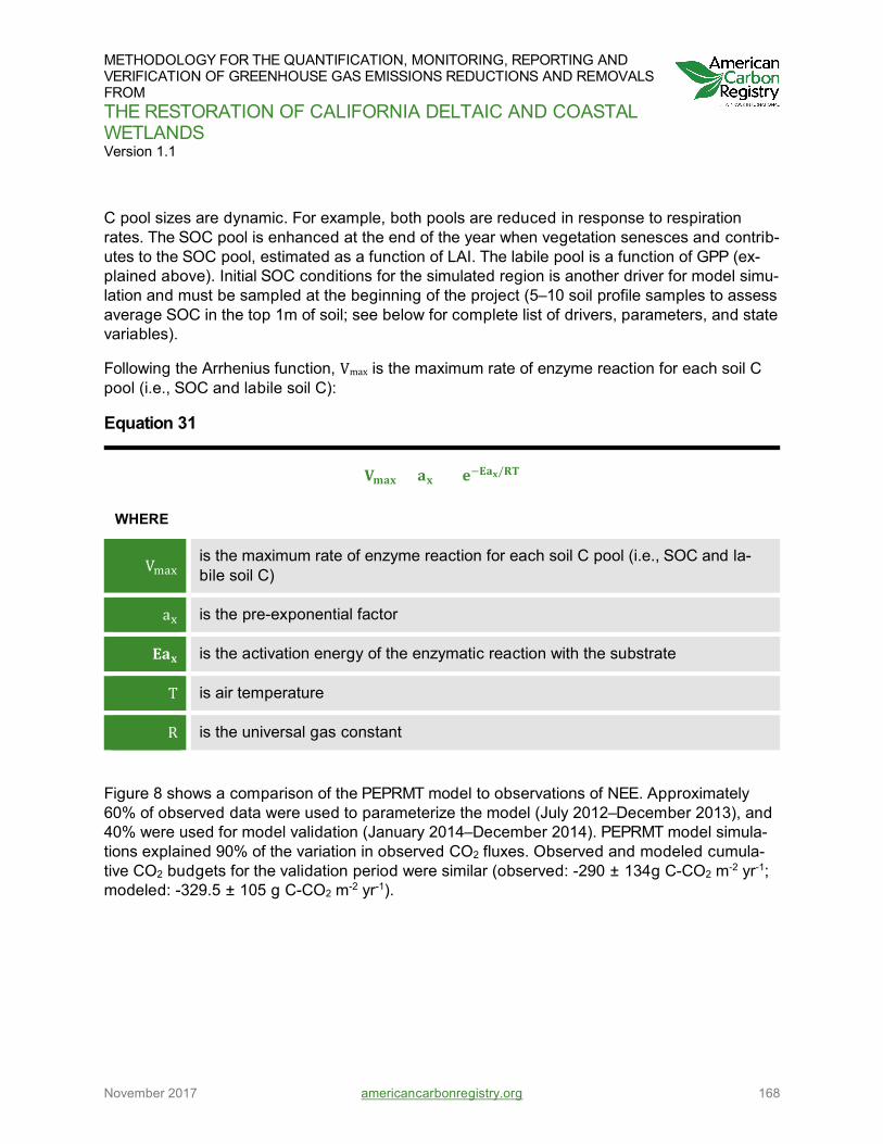
METHODOLOGY FOR THE QUANTIFICATION, MONITORING, REPORTING AND VERIFICATION OF GREENHOUSE GAS EMISSIONS REDUCTIONS AND REMOVALS FROM THE RESTORATION OF CALIFORNIA DELTAIC AND COASTAL WETLANDS Version 1.1
November 2017 americancarbonregistry.org 168
C pool sizes are dynamic. For example, both pools are reduced in response to respiration rates. The SOC pool is enhanced at the end of the year when vegetation senesces and contrib-utes to the SOC pool, estimated as a function of LAI. The labile pool is a function of GPP (ex-plained above). Initial SOC conditions for the simulated region is another driver for model simu-lation and must be sampled at the beginning of the project (5–10 soil profile samples to assess average SOC in the top 1m of soil; see below for complete list of drivers, parameters, and state variables).
Following the Arrhenius function, Vmax is the maximum rate of enzyme reaction for each soil C pool (i.e., SOC and labile soil C):
Equation 31
𝐕𝐕𝐞𝐞𝐚𝐚𝐞𝐞 = 𝐚𝐚𝐞𝐞 × 𝐀𝐀−𝐄𝐄𝐚𝐚𝐞𝐞/𝐀𝐀𝐄𝐄
WHERE
Vmax is the maximum rate of enzyme reaction for each soil C pool (i.e., SOC and la-bile soil C)
ax is the pre-exponential factor
𝐄𝐄𝐚𝐚𝐞𝐞 is the activation energy of the enzymatic reaction with the substrate
T is air temperature
R is the universal gas constant
Figure 8 shows a comparison of the PEPRMT model to observations of NEE. Approximately 60% of observed data were used to parameterize the model (July 2012–December 2013), and 40% were used for model validation (January 2014–December 2014). PEPRMT model simula-tions explained 90% of the variation in observed CO2 fluxes. Observed and modeled cumula-tive CO2 budgets for the validation period were similar (observed: -290 ± 134g C-CO2 m-2 yr-1; modeled: -329.5 ± 105 g C-CO2 m-2 yr-1).

METHODOLOGY FOR THE QUANTIFICATION, MONITORING, REPORTING AND VERIFICATION OF GREENHOUSE GAS EMISSIONS REDUCTIONS AND REMOVALS FROM THE RESTORATION OF CALIFORNIA DELTAIC AND COASTAL WETLANDS Version 1.1
November 2017 americancarbonregistry.org 169
Figure 8: Comparison of PEPRMT Model to Observations of NEE
(a) PEPRMT modeled and observed net ecosystem exchange of CO2 (NEE) from July 2012 to December 2014 at West Pond wetland. Data to the left of the black vertical line were used in model parameterization and data to the right were used in model validation. (
b) Data model agreement was high during the parameterization period (param) (slope=1, inter-cept=0.26; r2 = 0.92; RMSE = 0.85) and during the validation period (valid) (slope=1, inter-cept=0.13; r2 = 0.90; RMSE = 0.86).
(c) Similar integrated observed and modeled NEE fluxes were observed during the validation period (observed: -290 ± 134g C-CO2 m-2 yr-1; modeled: -329.5 ± 105 g C-CO2 m-2 yr-1) as well as across the entire observation period (observed: -1220.6 ± 336g C-CO2 m-2 yr-1; modeled: -1107.0 ± 257 g C-CO2 m-2 yr-1). Errors are 90% confidence intervals. Observed error is the sum of random and gap-filling errors. Model error is calculated based on variance across accepted posterior model parameters.

METHODOLOGY FOR THE QUANTIFICATION, MONITORING, REPORTING AND VERIFICATION OF GREENHOUSE GAS EMISSIONS REDUCTIONS AND REMOVALS FROM THE RESTORATION OF CALIFORNIA DELTAIC AND COASTAL WETLANDS Version 1.1
November 2017 americancarbonregistry.org 170
In order to predict net CH4 emissions, both CH4 oxidation and production need to be simu-lated. Again, we employ a simple model based on enzyme kinetics where CH4 production is a function of the size and availability of two soil C pools, temperature, and water table height, and CH4 oxidation is a function of the availability of CH4, temperature, and water table height. Both processes are predicted to increase exponentially with temperature. However, high water table conditions enhance CH4 production and limit oxidation, and low water table heights in-hibit CH4 production and increase oxidation. Two transport pathways are also modeled: plant–mediated CH4 transport and hydrodynamic CH4 flux. Both of these transport pathways are de-pendent on water table height and concentration gradients of CH4 between the water and at-mosphere. Plant-mediated transport is also a function of GPP (Sturtevant et al. 2016; Poindex-ter et al. 2016).
The biogeochemical model for CH4 production and oxidation is based on the DAMM model foundation. Similar to the Reco DAMM model, CH4 production is predicted using an Arrhenius equation paired with Michaelis-Menten equations estimating the concentration of two C sub-strates at the enzyme reaction site.
𝐀𝐀𝚫𝚫𝐟𝐟𝟎𝟎 =𝐕𝐕𝐞𝐞𝐚𝐚𝐞𝐞𝐚𝐚𝐚𝐚𝐛𝐛𝐞𝐞𝐚𝐚𝐀𝐀 × [𝚫𝚫𝐚𝐚𝐚𝐚𝐛𝐛𝐞𝐞𝐚𝐚𝐀𝐀]𝐤𝐤𝐌𝐌𝐚𝐚𝐚𝐚𝐛𝐛𝐞𝐞𝐚𝐚𝐀𝐀 + [𝚫𝚫𝐚𝐚𝐚𝐚𝐛𝐛𝐞𝐞𝐚𝐚𝐀𝐀] ×
𝐕𝐕𝐞𝐞𝐚𝐚𝐞𝐞𝐁𝐁𝐎𝐎𝚫𝚫 × [𝚫𝚫𝐁𝐁𝐎𝐎𝚫𝚫]𝐤𝐤𝐌𝐌𝐁𝐁𝐎𝐎𝚫𝚫 + [𝚫𝚫𝐁𝐁𝐎𝐎𝚫𝚫] × 𝐟𝐟(𝐒𝐒𝐄𝐄)
To account for the inhibition of CH4 production by the presence of O2, an O2 effect parameter is applied when the water table falls below the soil surface. Previous research has indicated that CH4 production rates can take multiple days to recover following re-saturation, due to the slow recharge of alternative electron acceptors (Kettunen et al. 1999; Moore and Dalva 1993). A previous analysis at the West Pond wetland confirmed that lowering the water table can have sustained negative effects on CH4 emission, lasting up to 20 days (Sturtevant et al. 2016). We added a lag effect into the model, where CH4 production is inhibited for 20 days following a drop in the water table.
CH4 oxidation also follows the DAMM model foundation, where CH4 is the only substrate
𝐎𝐎𝚫𝚫𝐟𝐟𝟎𝟎 =𝐕𝐕𝐞𝐞𝐚𝐚𝐞𝐞𝚫𝚫𝐟𝐟𝟎𝟎 × [𝚫𝚫𝐟𝐟𝟎𝟎]𝐤𝐤𝐌𝐌𝚫𝚫𝐟𝐟𝟎𝟎 + [𝚫𝚫𝐟𝐟𝟎𝟎] × 𝐟𝐟(𝐒𝐒𝐄𝐄)
To account for the inhibition of CH4 oxidation when the water table is above the soil surface, a water table function (f (WT)) is applied when the water table is above the soil surface.
Hydrodynamic flux is predicted using the Poindexter model, which was parameterized and val-idated at the same mature wetland site as the model described here (Poindexter et al. 2016). This predicts transfer of CH4 stored in the water directly to the atmosphere given the concen-tration gradient between CH4 in water and CH4 in the atmosphere as well as a gas transfer ve-locity:
𝐁𝐁𝐡𝐡𝐲𝐲𝐀𝐀𝐚𝐚𝐞𝐞 = 𝐤𝐤𝐡𝐡𝐲𝐲𝐀𝐀𝐚𝐚𝐞𝐞 × ([𝚫𝚫𝐟𝐟𝟎𝟎𝐰𝐰𝐚𝐚𝐚𝐚𝐀𝐀𝐚𝐚]− [𝚫𝚫𝐟𝐟𝟎𝟎𝐀𝐀𝐚𝐚𝐚𝐚𝐟𝐟𝐚𝐚𝐚𝐚𝐀𝐀])

METHODOLOGY FOR THE QUANTIFICATION, MONITORING, REPORTING AND VERIFICATION OF GREENHOUSE GAS EMISSIONS REDUCTIONS AND REMOVALS FROM THE RESTORATION OF CALIFORNIA DELTAIC AND COASTAL WETLANDS Version 1.1
November 2017 americancarbonregistry.org 171
Where khydro is the gas transfer velocity through the water (0.04 m d-1). Concentrations of CH4 in the water or soil ([CH4water]; µmol m-3) are modeled based on production and oxidation rates of CH4. After accounting for CH4 solubility in water, dissolved concentrations of methane at the surface ([CH4surface]; µmol m-3) are so small they are assumed to be zero.
Plant-mediated flux is predicted following the Dynamic Land Ecosystem Model (DLEM) (Tian et al. 2010). This predicts plant-mediated transport of CH4 given the concentration gradient be-tween CH4 in water and CH4 in the atmosphere as well as plant transport efficiency and plant activity:
𝐁𝐁𝐓𝐓𝐚𝐚𝐚𝐚𝐞𝐞𝐚𝐚 = (𝐤𝐤𝐓𝐓𝐚𝐚𝐚𝐚𝐞𝐞𝐚𝐚 × ([𝚫𝚫𝐟𝐟𝟎𝟎𝐰𝐰𝐚𝐚𝐚𝐚𝐀𝐀𝐚𝐚] − [𝚫𝚫𝐟𝐟𝟎𝟎𝐚𝐚𝐚𝐚𝐞𝐞]) ×𝐟𝐟𝐏𝐏𝐏𝐏
𝐟𝐟𝐏𝐏𝐏𝐏𝐞𝐞𝐚𝐚𝐞𝐞 ) × 𝐕𝐕𝐞𝐞𝐞𝐞𝐞𝐞
where kplant is the gas transfer velocity through plants, assumed to be constant (0.24 m d-1) (Moore and Dalva 1993). Concentrations of CH4 in the soil and water ([CH4water]; µmol m-3) are modeled based on production and oxidation rates of CH4. Again, after accounting for CH4 sol-ubility in water, dissolved concentrations of CH4 in the atmosphere ([CH4atm]; µmol m-3) are so small, they are assumed to be zero. Plant activity is assessed using GPP, where the most plant transport is expected to occur when GPP is at its highest point. Finally, a fraction of CH4 trans-ported through plants is assumed to be oxidized at a constant rate (Voxi =0.35) (van der Nat and Middelburg, 1998b).
Figure 9 compares the PEPRMT modeled CH4 flux in West Pond Wetland. PEPRMT model sim-ulations explained 65% of the variation in observed CH4 fluxes. Observed and modeled cumu-lative CH4 budgets for the validation period were very similar (observed: 40.3 ± 4.5 g C-CH4 m-
2 yr-1; modeled: 40.4 ± 2.8 g C- CH4 m-2 yr-1).
Figure 9: Comparison of PEPRMT Model to Observations of CH4.
(a) PEPRMT modeled and observed ecosystem exchange of CH4 in West Pond wetland. Data to the left of the black vertical line were used in model parameterization and data to the right were used in model validation. (b) Data-model agreement was high during the parameteriza-tion period (param) (slope = 0.76, intercept = 31; r2 = 0.60; RMSE = 48.6) and during the vali-dation period (valid) (slope = 0.7, intercept = 33; r2 = 0.67; RMSE = 57.2). (c) Similar inte-grated observed and modeled CH4 fluxes were observed during the parameterization period (observed: 47.9 ± 6 g C- CH4 m-2; modeled: 41.0 ± 3.0 g C- CH4 m-2) and validation period (ob-served: 40.3 ± 4.5 g C- CH4 m-2 yr-1; modeled: 40.4 ± 2.8 g C- CH4 m-2 yr-1). Across the entire observation period budgets were similar (observed: 88.2± 10.5 g C- CH4 m-2; modeled: 81.4± 6.0 6 g C- CH4 m-2). Errors are 90% confidence intervals. Observed error is the sum of random and gap-filling errors.

METHODOLOGY FOR THE QUANTIFICATION, MONITORING, REPORTING AND VERIFICATION OF GREENHOUSE GAS EMISSIONS REDUCTIONS AND REMOVALS FROM THE RESTORATION OF CALIFORNIA DELTAIC AND COASTAL WETLANDS Version 1.1
November 2017 americancarbonregistry.org 172
Model error is calculated based variance across accepted posterior model parameters.
DATA UNIT/PARAMETER METEOROLOGICAL DATA
Description Air temperature and in-coming radiation
Units Degree Celsius and µmol radiation m-2 s-1
Data source California Irrigation Management Information System (CIMIS) website (http://wwwcimis.water.ca.gov/cimis/data.jsp)

METHODOLOGY FOR THE QUANTIFICATION, MONITORING, REPORTING AND VERIFICATION OF GREENHOUSE GAS EMISSIONS REDUCTIONS AND REMOVALS FROM THE RESTORATION OF CALIFORNIA DELTAIC AND COASTAL WETLANDS Version 1.1
November 2017 americancarbonregistry.org 173
Frequency of monitoring/recording
30 min
DATA UNIT/PARAMETER INITIAL SOIL ORGANIC CARBON
Description Amount of existing soil organic carbon at beginning of Project
Units g C m-3 soil
Data source Direct sampling (5-10 soil profile samples averaged across top 1m soil; replicate spatially as needed) is recommended. Soil organic carbon can be accurately estimated from loss on ignition using data presented Callaway et al. (2012) and Drexler et al. (2009).
Description of measure-ment methods and proce-
dures to be applied
If data from NRCS SSURGO is used, the uncertainty in the spatial resolution of soils properties (including soil organic matter) must be accounted for in model inputs
Frequency of monitoring/recording
Once at beginning of Project
DATA UNIT/PARAMETER WATER TABLE HEIGHT
Description Distance from surface of soil to water table—for Project conditions
Units cm
Data source Direct or automated measurement
Description of measure-ment methods and proce-
dures to be applied
Measure by hand distance of water height to soil surface or install pressure transducer to continuously monitor water ta-ble height (such as Campbell Scientific CS451-L)
Frequency of monitoring/recording
Daily-weekly

METHODOLOGY FOR THE QUANTIFICATION, MONITORING, REPORTING AND VERIFICATION OF GREENHOUSE GAS EMISSIONS REDUCTIONS AND REMOVALS FROM THE RESTORATION OF CALIFORNIA DELTAIC AND COASTAL WETLANDS Version 1.1
November 2017 americancarbonregistry.org 174
Description Distance from surface of soil to water table—for Project conditions
DATA UNIT/PARAMETER LEAF AREA INDEX
Description One-sided green leaf area per ground surface area
Units m2 leaf area m-2 ground area
Data source Destructive field sampling, LAI sensor (e.g., LAI-2200C Plant Canopy Analyzer), or remote sensing
Description of measure-ment methods and proce-
dures to be applied
Destructive sampling: remove all leaves in a known surface area (e.g.40 cm x 40 cm), measure leaf area of all removed leaves. Repeat across landscape (ideally 5 measurements per plant cover type).
LAI sensor: collect 10 measurements along a transect through each plant cover type
Remote sensing: Phenocams, or digital cameras that are au-tomated to record images of canopy cover throughout the year, can be used to calculate a greenness index (GI) that can be empirically related to LAI based on field measure-ments (Richardson et al. 2009, Ryu et al. 2012, Sonnentag et al. 2011). Other forms of remote sensing may also be availa-ble such as satellite images provided by MODIS.
Frequency of monitoring/recording
Measurements must be collected frequently during the grow-ing season; measurements during the non-growing seasons are also required
QA/QC procedures See Methods Module (MM-W/RC)

METHODOLOGY FOR THE QUANTIFICATION, MONITORING, REPORTING AND VERIFICATION OF GREENHOUSE GAS EMISSIONS REDUCTIONS AND REMOVALS FROM THE RESTORATION OF CALIFORNIA DELTAIC AND COASTAL WETLANDS Version 1.1
November 2017 americancarbonregistry.org 175
Photosynthesis PEPRMT Model Parameters, Descriptions, and Values
PARAMETERS, STATE
VARIABLES, AND DRIVER VARIABLES
DESCRIPTION VALUE
PARAMETERS
ε Light use efficiency (g C MJ-1) 0.94
Ha Activation energy for photosynthesis (kJ mol-1) 21.5
Hd Inhibition of photosynthesis at high temperatures (kJ mol-1)
110
R Universal gas constant 0.00831
Topt Optimum temp for photosynthesis 25ºC
STATE VARIABLES
NEE Net ecosystem exchange CO2 (µmol m-2 s-1)
GPP Gross ecosystem primary productivity (µmol m-2 s-1)
DRIVER VARIABLES
Air temperature ºC
PAR Photosynthetically active radiation (µmol m-2 s-1)
LAI Leaf area index

METHODOLOGY FOR THE QUANTIFICATION, MONITORING, REPORTING AND VERIFICATION OF GREENHOUSE GAS EMISSIONS REDUCTIONS AND REMOVALS FROM THE RESTORATION OF CALIFORNIA DELTAIC AND COASTAL WETLANDS Version 1.1
November 2017 americancarbonregistry.org 176
Respiration PEPRMT Model Parameters, Descriptions, and Values
PARAMETERS, STATE
VARIABLES, AND DRIVER VARIABLES
DESCRIPTION VALUE
PARAMETERS
kMlabile Michaelis-Menten constant for labile C (g C cm-3 soil) 1.7 x 10⁻⁶
kMSOC Michaelis-Menten constant for SOC (g C cm-3 soil) 6.3 x 10⁻⁶
αlabile Pre-exponential factor for labile C (µmol C cm-3 soil s-1) 2
αSOC Pre-exponential factor for SOC (µmol C cm-3 soil s-1) 2
Ealabile Activation energy for labile C (kJ mol-1) 18
EaSOC Activation energy for SOC (kJ mol-1) 17.8
CSOC Initial SOC pool (mol C m-3) measured
STATE VARIABLES
Reco Ecosystem respiration (µmol m-2 s-1)
CSOC SOC pool
DRIVER VARIABLES
Air temperature ºC
PAR Photosynthetically active radiation (µmol m-2 s-1)
WT Water table height
GPP Gross ecosystem primary productivity (µmol m-2 s-1)

METHODOLOGY FOR THE QUANTIFICATION, MONITORING, REPORTING AND VERIFICATION OF GREENHOUSE GAS EMISSIONS REDUCTIONS AND REMOVALS FROM THE RESTORATION OF CALIFORNIA DELTAIC AND COASTAL WETLANDS Version 1.1
November 2017 americancarbonregistry.org 177
CH4 PEPRMT Model Parameters, Descriptions, and Values
PARAMETERS, STATE
VARIABLES, AND DRIVER VARIABLES
DESCRIPTION VALUE
PARAMETERS
kMlabile
Michaelis-Menten constant for labile C (g C cm-3 soil) 2.3 x 10⁻⁵
kMSOC Michaelis-Menten constant for SOC (g C cm-3 soil) 1.7 x 10⁻⁵
kMCH4 Michaelis-Menten constant for CH4 oxidation (g C cm-3 soil)
2.3 x 10⁻⁵
αlabile Pre-exponential factor for labile C (µmol C cm-3 soil s-1) 6 x 10⁸
αSOC Pre-exponential factor for SOC (µmol C cm-3 soil s-1) 6 x 10⁷
aCH4 Pre-exponential factor for CH4 oxidation (µmol C cm-3 soil s-1)
6 x 10⁷
Ealabile Activation energy for labile C (kJ mol-1) 71.1
EaSOC Activation energy for SOC (kJ mol-1) 67.1
EaCH4 Activation energy for CH4 oxidation (kJ mol-1) 75.4
CSOC Initial SOC pool (mol C m-3) measured
kplant Gas transfer velocity through plants (Kettunen et al. 2003)
0.24 m d-1
Voxi Fraction of CH4 oxidized during plant transport 0.35
khydro Gas transfer velocity through water (Poindexter et al. 2016)
0.04 m d-1
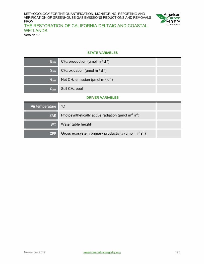
METHODOLOGY FOR THE QUANTIFICATION, MONITORING, REPORTING AND VERIFICATION OF GREENHOUSE GAS EMISSIONS REDUCTIONS AND REMOVALS FROM THE RESTORATION OF CALIFORNIA DELTAIC AND COASTAL WETLANDS Version 1.1
November 2017 americancarbonregistry.org 178
STATE VARIABLES
RCH4 CH4 production (µmol m-2 d-1)
OCH4 CH4 oxidation (µmol m-2 d-1)
NCH4 Net CH4 emission (µmol m-2 d-1)
CCH4 Soil CH4 pool
DRIVER VARIABLES
Air temperature ºC
PAR Photosynthetically active radiation (µmol m-2 s-1)
WT Water table height
GPP Gross ecosystem primary productivity (µmol m-2 s-1)

METHODOLOGY FOR THE QUANTIFICATION, MONITORING, REPORTING AND VERIFICATION OF GREENHOUSE GAS EMISSIONS REDUCTIONS AND REMOVALS FROM THE RESTORATION OF CALIFORNIA DELTAIC AND COASTAL WETLANDS Version 1.1
November 2017 americancarbonregistry.org 179
Anderson, F. E., Bergamaschi, B., Sturtevant, C., Knox, S., Hastings, L., Windham-Myers, L., et al. (2016). Variation of energy and carbon fluxes from a restored temperate freshwater wetland and implications for carbon market verification protocols. Journal of Geophysical Research: 121, 777–795. DOI: 10.1002/2015JG003083
Assa, Y., & Horwath W. (2011). Report on GHG emissions study in Twitchell Island in Corn and Rice Systems conducted in Spring 2010-Fall 2011.
Aubinet, M., Berbigier, P., Bernhofer, C., Cescatti, A., Feigenwinter, C., Granier, A., et al. (2005). Comparing CO2 storage and advection conditions at night at different carboeuroflux sites. Boundary-Layer Meteorology, 116(1), 63–93. https://doi.org/10.1007/s10546-004-7091-8
Badiou, P., McDougal, R., Pennock, D., & Clark, B. (2011). Greenhouse gas emissions and carbon sequestration potential in restored wetlands of the Canadian prairie pothole region. Wetlands Ecology and Management, 19(3), 237–256. https://doi.org/10.1007/s11273-011-9214-6
Baldocchi, D. D., Hincks, B. B., & Meyers, T. P. (1988). Measuring biosphere-atmosphere ex-changes of biologically related gases with micrometeorological methods. Ecology, 69(5), 1331–1340. https://doi.org/10.2307/1941631
Baldocchi, D., Detto, M., Sonnentag, O., Verfaillie, J., Teh, Y. A., Silver, W., & Kelly, N. M. (2012). The challenges of measuring methane fluxes and concentrations over a peatland pas-ture. Agricultural and Forest Meteorology, 153, 177–187. https://doi.org/10.1016/j.agrformet.2011.04.013
Ball, D. F. (1964). Loss-on-ignition as an estimate of organic matter and organic carbon in non-calcareous soils. Journal of Soil Science, 15(1), 84–92. https://doi.org/10.1111/j.1365-2389.1964.tb00247.x
Bates, L. A. (1977). Soil Survey of Solano County, California. U.S. Dept. of Agriculture, Soil Conservation Service.
Bergamaschi, B. A., Fleck, J. A., Downing, B. D., Boss, E., Pellerin, B., Ganju, N. K., et al. (2011). Methyl mercury dynamics in a tidal wetland quantified using in situ optical measure-ments. Limnology and Oceanography, 56(4), 1355–1371. https://doi.org/10.4319/lo.2011.56.4.1355
Black, K., Bolger, T., Davis, P., Nieuwenhuis, M., Reidy, B., Saiz, G., et al. (2007). Inventory and eddy covariance-based estimates of annual carbon sequestration in a Sitka spruce (Picea sitchensis (Bong.) Carr.) forest ecosystem. European Journal of Forest Research, 126(2), 167–178. https://doi.org/10.1007/s10342-005-0092-4

METHODOLOGY FOR THE QUANTIFICATION, MONITORING, REPORTING AND VERIFICATION OF GREENHOUSE GAS EMISSIONS REDUCTIONS AND REMOVALS FROM THE RESTORATION OF CALIFORNIA DELTAIC AND COASTAL WETLANDS Version 1.1
November 2017 americancarbonregistry.org 180
Blake, G. R. (1965). Bulk density. Pp. 374–390 (Chapter 30) in Methods of Soil Analysis. Part 1. Physical and Mineralogical Properties, Including Statistics of Measurement and Sampling, Agronomy Monograph 9.1. https://dl.sciencesocieties.org/publications/books/abstracts/agron-omymonogra/methodsofsoilana/374/preview
Blake, G. R., and Hartge, K.H. (1986). Bulk Density in Methods of Soil Analysis, Part I. Physical and Mineralogical Methods: Agronomy Monograph no.9 (2nd ed.). A. Klute, ed. Madison, WI. American Society of Agronomy and Soil Science Society of America. pp. 363-375.
Bonan, G. B., Hartman, M. D., Parton, W. J., & Wieder, W. R. (2013). Evaluating litter decompo-sition in earth system models with long-term litterbag experiments: An example using the Com-munity Land Model version 4 (CLM4). Global Change Biology, 19(3), 957–974. https://doi.org/10.1111/gcb.12031
Bricker-Urso, S., Nixon, S. W., Cochran, J. K., Hirschberg, D. J., & Hunt, C. (1989). Accretion rates and sediment accumulation in Rhode Island salt marshes. Estuaries, 12(4), 300. https://doi.org/10.2307/1351908
Brock, B. (2011, June). Engineer, California Department of Water Resources, personal commu-nication.
Butterbach-Bahl, K., Baggs, E. M., Dannenmann, M., Kiese, R., & Zechmeister-Boltenstern, S. (2013.) Nitrous oxide emissions from soils: How well do we understand the processes and their controls. Philosophical Transactions of the Royal Society B: Biological Sciences, 368. DOI: 10.1098/rstb.2013.0122
Cahoon, D. R., & Turner, R. E. (1989). Accretion and canal impacts in a rapidly subsiding Wet-land II. Feldspar Marker Horizon Technique. Estuaries, 12(4), 260. https://doi.org/10.2307/1351905
Callaway, J. C., Borgnis, E. L., Turner, R. E., & Milan, C. S. (2012). Carbon sequestration and sediment accretion in San Francisco Bay tidal wetlands. Estuaries and Coasts, 35(5), 1163–1181. https://doi.org/10.1007/s12237-012-9508-9
Callaway, J. C., Parker, V. T., Vasey, M. C., Schile, L. M., & Herbert, E. R. (2011). Tidal wetland restoration in San Francisco Bay: History and current issues. San Francisco Estuary and Water-shed Science, 9(3). https://doi.org/10.15447/sfews.2011v9iss3art2
Canivari, M., Klonsky, K. M., & DeMoura, R. L. (2007). Sample costs to produce rice in 2007 for the Delta Region for continuous rice culture. University of California Cooperative Extension.
Canuel, E. A., Lerberg, E. J., Dickhut, R. M., Kuehl, S. A., Bianchi, T. S., & Wakeham, S. G. (2009). Changes in sediment and organic carbon accumulation in a highly-disturbed ecosys-tem: The Sacramento-San Joaquin River Delta (California, USA). Marine Pollution Bulletin, 59(4–7), 154–163. https://doi.org/10.1016/j.marpolbul.2009.03.025

METHODOLOGY FOR THE QUANTIFICATION, MONITORING, REPORTING AND VERIFICATION OF GREENHOUSE GAS EMISSIONS REDUCTIONS AND REMOVALS FROM THE RESTORATION OF CALIFORNIA DELTAIC AND COASTAL WETLANDS Version 1.1
November 2017 americancarbonregistry.org 181
Chappell, S. (2006, November). Suisun Marsh Resource Conservation District, personal com-munication.
Chauhan, R., Ramanathan, A. L., & Adhya, T. K. (2008). Assessment of methane and nitrous oxide flux from mangroves along Eastern coast of India. Geofluids, 8(4), 321–332.
Christiansen, J.R., Outhwaite, J. and Smukler, S.M. (2015). Comparison of CO2, CH4 and N2O soil-atmosphere exchange measured in static chambers with cavity ring-down spectroscopy and gas chromatography. Agricultural and Forest Meteorology, 211, 48–57.
Couwenberg, J., & Hooijer, A. (2013). Towards robust subsidence-based soil carbon emission factors for peat soils in south-east Asia, with special reference to oil palm plantations. Mires and Peat, 12(01), 1–13.
Couwenberg, J., Thiele, A., Tanneberger, F., Augustin, J., Bärisch, S., & Dubovik, D. (2011). Assessing greenhouse gas emissions from peatlands using vegetation as a proxy. Hydrobiolo-gia, 674, 67-89.
Craft, C. B., Seneca, E. D., & Broome, S. W. (1991). Loss on ignition and Kjeldahl digestion for estimating organic carbon and total nitrogen in estuarine marsh soils: Calibration with dry com-bustion. Estuaries and Coasts, 14(2), 175–179.
Crill, P. M., Butler, J. H., Cooper, D. J., & Novelli, P. C. (1995). Standard analytical methods for measuring trace gases in the environment. Biogenic Trace Gases: Measuring Emissions from Soil and Water, 164–205.
Davidson, E. A., Samanta, S., Caramori, S. S., & Savage, K. (2012). The Dual Arrhenius and Michaelis–Menten kinetics model for decomposition of soil organic matter at hourly to seasonal time scales. Global Change Biology, 18(1), 371–384.
Deverel, S. J., & Leighton, D. A. (2010). Historic, recent, and future subsidence, Sacramento-San Joaquin Delta, California, USA. San Francisco Estuary and Watershed Science, 8(2). https://escholarship.org/uc/item/7xd4x0xw.pdf
Deverel, S. J., & Rojstaczer, S. (1996). Subsidence of agricultural lands in the Sacramento-San Joaquin Delta, California: Role of aqueous and gaseous carbon fluxes. Water Resources Re-search 32(8), 2359–2367.
Deverel, S. J., Ingrum, T., & Leighton, D. (2016). Present-day oxidative subsidence of organic soils and mitigation in the Sacramento-San Joaquin Delta, California, USA. Hydrogeology Jour-nal, 24(3), 569–586.
Deverel, S. J., Leighton, D. A., & Finlay, M. R. (2007). Processes affecting agricultural drainwa-ter quality and organic carbon loads in California’s Sacramento–San Joaquin Delta. San Fran-cisco Estuary and Watershed Science, 5(2). https://escholarship.org/uc/item/8db266mg.pdf

METHODOLOGY FOR THE QUANTIFICATION, MONITORING, REPORTING AND VERIFICATION OF GREENHOUSE GAS EMISSIONS REDUCTIONS AND REMOVALS FROM THE RESTORATION OF CALIFORNIA DELTAIC AND COASTAL WETLANDS Version 1.1
November 2017 americancarbonregistry.org 182
Deverel, S. J., Lucero, C. E., & Bachand, S. (2015). Evolution of arability and land use, Sacra-mento–San Joaquin Delta, California. San Francisco Estuary and Watershed Science, 13(2). https://escholarship.org/uc/item/5nv2698k.pdf
Deverel, S. J., Wang, B., & Rojstaczer, S. A. (1998). Subsidence in the Sacramento-San Joaquin Delta. Pp. 489-502 in Proceedings of the Joseph Poland Subsidence Symposium, J. W. Borchers (ed.). Association of Engineering Geologists, Special Publication No. 8. Belmont, CA: Star Publishing.
Dore, S., Hymus, G. J., Johnson, D. P., Hinkle, C. R., Valentini, R., & Drake, B. G. (2003). Cross validation of open-top chamber and eddy covariance measurements of ecosystem CO2 ex-change in a Florida scrub-oak ecosystem. Global Change Biology, 9(1), 84–95.
Drexler, J. Z. (2011). Peat formation processes through the millennia in tidal marshes of the Sacramento–San Joaquin Delta, California, USA. Estuaries and Coasts, 34(5), 900.
Drexler, J. Z., de Fontaine, C. S., & Deverel, S. J. (2009). The legacy of wetland drainage on the remaining peat in the Sacramento–San Joaquin Delta, California, USA. Wetlands, 29(1), 372–386.
Eggleston, H. S., Buendia, L., Miwa, K., Ngara, T., & Tanabe, K. (2006). IPCC guidelines for na-tional greenhouse gas inventories, prepared by the National Greenhouse Gas Inventories Pro-gramme, Institute for Global Environmental Strategies, Hayama, Japan.
ElSiddig, E. (2003). Good Practice Guidance for Land Use, Land-Use Change and Forestry. http://khartoumspace.uofk.edu/handle/123456789/6871
Espe, M. B., Kirk, E., van Kessel, C., Horwath, W. H., & Linquist, B. A. (2015). Indigenous nitro-gen supply of rice is predicted by soil organic carbon. Soil Science Society of America Journal, 79(2), 569–576. https://doi.org/10.2136/sssaj2014.08.0328
Falge, E., Baldocchi, D., Olson, R., Anthoni, P., Aubinet, M., Bernhofer, C., et al. (2001). Gap filling strategies for defensible annual sums of net ecosystem exchange. Agricultural and For-est Meteorology, 107(1), 43–69.
Ganju, N. K., Schoellhamer, D. H., & Bergamaschi, B. A. (2005). Suspended sediment fluxes in a tidal wetland: Measurement, controlling factors, and error analysis. Estuaries and Coasts, 28(6), 812–822.
Garrigues, S., Lacaze, R., Baret, F., Morisette, J. T., Weiss, M., Nickeson, J. E., et al. (2008). Validation and intercomparison of global Leaf Area Index products derived from remote sens-ing data. Journal of Geophysical Research: Biogeosciences, 113(G2). http://onlineli-brary.wiley.com/doi/10.1029/2007JG000635/full
Gatland, J. R., Santos, I. R., Maher, D. T., Duncan, T. M., & Erler, D. V. (2014). Carbon dioxide and methane emissions from an artificially drained coastal wetland during a flood: Implications

METHODOLOGY FOR THE QUANTIFICATION, MONITORING, REPORTING AND VERIFICATION OF GREENHOUSE GAS EMISSIONS REDUCTIONS AND REMOVALS FROM THE RESTORATION OF CALIFORNIA DELTAIC AND COASTAL WETLANDS Version 1.1
November 2017 americancarbonregistry.org 183
for wetland global warming potential. Journal of Geophysical Research: Biogeosciences, 119(8), 1698–1716.
Göckede, M., Markkanen, T., Hasager, C. B., & Foken, T. (2006). Update of a footprint-based approach for the characterisation of complex measurement sites. Boundary-Layer Meteorol-ogy, 118(3), 635–655.
Grieve, C. M., Grattan, S. R., & Maas, E. V. (2012). Plant salt tolerance. In Agricultural Salinity Assessment and Management, ASCE Manuals and Reports on Engineering Practice No. 71, Second Edition, W. W. Wallender and K. K. Tanji (eds.). New York: American Society of Civil Engineers.
Hargis, T. G., & Twilley, R. R. (1994). Improved coring device for measuring soil bulk density in a Louisiana deltaic marsh: Research method paper. Journal of Sedimentary Research, 64(3). http://archives.datapages.com/data/sepm/journals/v63-66/data/064a/064a003/0681.htm
Hatala, J. A., Detto, M., Sonnentag, O., Deverel, S. J., Verfaillie, J., & Baldocchi, D. D. (2012). Greenhouse gas (CO 2, CH 4, H 2 O) fluxes from drained and flooded agricultural peatlands in the Sacramento-San Joaquin Delta. Agriculture, Ecosystems & Environment, 150, 1–18.
Hirano, T., Segah, H., Kusin, K., Limin, S., Takahashi, H., & Osaki, M. (2012). Effects of disturb-ances on the carbon balance of tropical peat swamp forests. Global Change Biology, 18(11), 3410–3422.
Hollinger, S. E., Bernacchi, C. J., & Meyers, T. P. (2005). Carbon budget of mature no-till eco-system in North Central Region of the United States. Agricultural and Forest Meteorology, 130(1), 59–69.
Howard, J., Hoyt, S., Isensee, K., Telszewski, M., & Pidgeon, E. (eds.). (2014). Coastal blue carbon: Methods for assessing carbon stocks and emissions factors in mangroves, tidal salt marshes, and seagrasses. http://www.cifor.org/online-library/browse/view-publication/publica-tion/5095.html
Howitt, R. E., Medellin-Azuara, J., MacEwan, D. & Lund, J. R. (2012). Calibrating disaggregate economic models of agricultural production and water management. Environmental Modeling and Software, 38, 244-258.
Hutchinson, G. L., & Mosier, A. R. (1981). Improved soil cover method for field measurement of nitrous oxide fluxes. Soil Science Society of America Journal, 45(2), 311–316.
HydroFocus, Inc. (2007) Technical memorandum, recent and estimated future subsidence rates and land surface elevation changes in the Sacramento-San Joaquin Delta and Suisun Marsh, Delta Risk Management Strategy, Department of Water Resources, Sacramento, CA.

METHODOLOGY FOR THE QUANTIFICATION, MONITORING, REPORTING AND VERIFICATION OF GREENHOUSE GAS EMISSIONS REDUCTIONS AND REMOVALS FROM THE RESTORATION OF CALIFORNIA DELTAIC AND COASTAL WETLANDS Version 1.1
November 2017 americancarbonregistry.org 184
Intergovernmental Panel on Climate Change (IPCC). (2013). Chapter 3 in 2013 Supplement to the 2006 IPCC Guidelines for National Greenhouse Gas Inventories: Wetlands. http://www.ipcc-nggip.iges.or.jp/public/wetlands/
Jiang, Y., Tang, S., Wang, C., Zhou, P., Tenuta, M., Han, G., & Huang, D. (2012). Contribution of urine and dung patches from grazing sheep to methane and carbon dioxide fluxes in an In-ner Mongolian desert grassland. Asian-Australasian Journal of Animal Sciences, 25(2), 207–212. https://doi.org/10.5713/ajas.2011.11261
Kalra, Y. (1997). Handbook of Reference Methods for Plant Analysis. Boca Raton FL: CRC Press. https://books.google.com/books?hl=en&lr=&id=wLggXPmhY18C&oi=fnd&pg=PR3&dq=Hand-book+of+Reference+Methods+for+Plant+Analy-sis&ots=S5X93_LH91&sig=jr2Nl4QzVnKor4tlthButmItUIk
Kasimir-Klemedtsson, A., Klemedtsson, L., Berglund, K., Martikainen, P., Silvola, J., & Oenema, O. (1997). GHG emissions from farmed organic soils; a review. Soil Use and Management, 13, 245–250.
Keenan, T. F., Carbone, M. S., Reichstein, M., & Richardson, A. D. (2011). The model–data fu-sion pitfall: Assuming certainty in an uncertain world. Oecologia, 167(3), 587.
Kettunen, A., Kaitala, V., Lehtinen, A., Lohila, A., Alm, J., Silvola, J., & Martikainen, P. J. (1999). Methane production and oxidation potentials in relation to water table fluctuations in two boreal mires. Soil Biology and Biochemistry, 31(12), 1741–1749.
Klinger, L. F., Zimmerman, P. R., Greenberg, J. P., Heidt, L. E., & Guenther, A. B. (1994). Car-bon trace gas fluxes along a successional gradient in the Hudson Bay lowland. Journal of Geo-physical Research: Atmospheres, 99(D1), 1469–1494.
Knox, S. H., Sturtevant, C., Matthes, J. H., Koteen, L., Verfaillie, J., & Baldocchi, D. (2015). Ag-ricultural peatland restoration: Effects of land-use change on greenhouse gas (CO2 and CH4) fluxes in the Sacramento-San Joaquin Delta. Global Change Biology, 21(2), 750–765.
Kochendorfer, J., Castillo, E. G., Haas, E., Oechel, W. C., & Paw U, K. T. (2011). Net ecosys-tem exchange, evapotranspiration and canopy conductance in a riparian forest. Agricultural and Forest Meteorology, 151(5), 544–553.
Laenen, A., & Curtis, R. E. (1989). Accuracy of Acoustic Velocity Metering Systems for Meas-urement of Low Velocity in Open Channels. US Geological Survey, US Department of the Inte-rior. https://pubs.usgs.gov/wri/1989/4090/report.pdf
Li, C., Six. J., Horwath. W. R., & Salas W. (2014). Calibrating, Validating, and Implementing Process Models for California Agriculture Greenhouse Gas Emissions, Final Report to the Air Resources Board. February 27, 2014.

METHODOLOGY FOR THE QUANTIFICATION, MONITORING, REPORTING AND VERIFICATION OF GREENHOUSE GAS EMISSIONS REDUCTIONS AND REMOVALS FROM THE RESTORATION OF CALIFORNIA DELTAIC AND COASTAL WETLANDS Version 1.1
November 2017 americancarbonregistry.org 185
Liikanen, A., Sivennoinen, H., Karvo, A., Rantakokko, P., & Martikainen, P. J. (2009). Methane and nitrous oxide fluxes in two coastal wetlands in the northeastern Gulf of Bothnia, Baltic Sea. Boreal Environment Research, 14(3). http://search.ebscohost.com/login.aspx?direct=true&pro-file=ehost&scope=site&authtype=crawler&jrnl=12396095&AN=43292456&h=st%2FTieM0xG3JP0sOoQnifgC22pTgqe6Sa9gaVOhToLuxKyrHmgvAhjsvuyj4dPrpoynEaDoWV1%2BAihUf-TxVscQ%3D%3D&crl=c
Lindau, C. W., & DeLaune, R. D. (1991). Dinitrogen and nitrous oxide emission and entrapment in Spartina alterniflora saltmarsh soils following addition of N-15 labelled ammonium and ni-trate. Estuarine, Coastal and Shelf Science, 32(2), 161–172.
Linquist, B. A., Adviento-Borbe, M. A., Pittelkow, C. M., van Kessel, C., & van Groenigen, K. J. (2012). Fertilizer management practices and greenhouse gas emissions from rice systems: A quantitative review and analysis. Field Crops Research, 135, 10–21.
Liu, M., He, H., Yu, G., Luo, Y., Sun, X., & Wang, H. (2009). Uncertainty analysis of CO2 flux components in subtropical evergreen coniferous plantation. Science in China Series D: Earth Sciences, 52(2), 257–268.
Livingston, G. P., & Hutchinson, G. L. (1995). Enclosure-based measurement of trace gas ex-change: Applications and sources of error. Biogenic Trace Gases: Measuring Emissions from Soil and Water, 14–51.
Loomis, R. S., & Connor, D. J. (1992). Crop Ecology: Productivity and Management in Agricul-tural Systems. Cambridge, UK: Cambridge University Press.
Lynch, J. C., Hensel, P., & Cahoon, D. R. (2015). The Surface Elevation Table and Marker Hori-zon Technique: A Protocol for Monitoring Wetland Elevation Dynamics (Federal Government Series No. NPS/NCBN/NRR—2015/1078). National Park Service. http://pubs.er.usgs.gov/publication/70160049
MacEwan, D., & Hatchett, S. (2012). Statewide Agricultural Production Model Update and Ap-plication to Federal Feasibility Analysis. Prepared for Bureau of Reclamation Mid-Pacific Re-gion, US Department of the Interior.
Macreadie, P. I., Baird, M. E., Trevathan-Tackett, S. M., Larkum, A. W. D., & Ralph, P. J. (2014). Quantifying and modelling the carbon sequestration capacity of seagrass meadows—a critical assessment. Marine Pollution Bulletin, 83(2), 430–439. https://doi.org/10.1016/j.marpol-bul.2013.07.038
Majumdar, D. (2013). Biogeochemistry of N2O uptake and consumption in submerged soils and rice fields and implications in climate change. Critical Reviews in Environmental Science and Technology, 43(24), 2653–2684. https://doi.org/10.1080/10643389.2012.694332

METHODOLOGY FOR THE QUANTIFICATION, MONITORING, REPORTING AND VERIFICATION OF GREENHOUSE GAS EMISSIONS REDUCTIONS AND REMOVALS FROM THE RESTORATION OF CALIFORNIA DELTAIC AND COASTAL WETLANDS Version 1.1
November 2017 americancarbonregistry.org 186
Massman, W. J. (2000). A simple method for estimating frequency response corrections for eddy covariance systems. Agricultural and Forest Meteorology, 104(3), 185–198. https://doi.org/10.1016/S0168-1923(00)00164-7
McGeehan, S. L., & Naylor, D. V. (1988). Automated instrumental analysis of carbon and nitro-gen in plant and soil samples. Communications in Soil Science and Plant Analysis, 19(4), 493–505. https://doi.org/10.1080/00103628809367953
McGlathery, K. J., Reynolds, L. K., Cole, L. W., Orth, R. J., Marion, S. R., & Schwarzschild, A. (2012). Recovery trajectories during state change from bare sediment to eelgrass dominance. Marine Ecology Progress Series, 448, 209–221.
McNicol, G., & Silver, W. L. (2014). Separate effects of flooding and anaerobiosis on soil green-house gas emissions and redox sensitive biogeochemistry. Journal of Geophysical Research: Biogeosciences, 119(4), 557–566. https://doi.org/10.1002/2013JG002433
Merrill A., Siegel S., Morris, B., Ferguson, A., Young, G., Ingram, C., et al. (2010). Greenhouse Gas Reduction and Environmental Benefits in the Sacramento-San Joaquin Delta: Advancing Carbon Capture Wetland Farms and Exploring Potential for Low Carbon Agriculture. Prepared for The Nature Conservancy, Sacramento, California. http://www.stillwatersci.com/
Medlyn, B. E., Dreyer, E., Ellsworth, D., Forstreuter, M., Harley, P. C., Kirschbaum, M. U. F., et al. (2002). Temperature response of parameters of a biochemically based model of photosyn-thesis. II. A review of experimental data. Plant, Cell & Environment, 25(9), 1167–1179. https://doi.org/10.1046/j.1365-3040.2002.00891.x
Megonigal, J. P., Hines, M. E., & Visscher, P. T. (2004). Anaerobic metabolism: Linkages to trace gases and aerobic processes. Pp. 317-424 in Biogeochemistry, W. H. Schlesinger (ed.). Oxford, UK: Elsevier-Pergamon.
Miller, R. L., (2011). Carbon gas fluxes in re-established wetlands on organic soils differ rela-tive to plant community and hydrology. Wetlands doi 10.1007/s13157-011-0215-2.
Miller, R. L., & Fujii, R. (2010). Plant community, primary productivity, and environmental condi-tions following wetland re-establishment in the Sacramento-San Joaquin Delta, California. Wet-lands Ecology and Management, 18(1), 1–16. https://doi.org/10.1007/s11273-009-9143-9
Miller, R. L., Fram, M., Fujii, R., & Wheeler, G. (2008). Subsidence reversal in a re-established wetland in the Sacramento-San Joaquin Delta, California, USA. San Francisco Estuary and Wa-tershed Science, 6(3). http://escholarship.org/uc/item/5j76502x
Miller, R. L., Hastings, L., & Fujii, R. (2000). Hydrologic Treatments Affect Gaseous Carbon Loss From Organic Soils, Twitchell Island, California, October 1995-December 1997 (USGS Numbered Series No. 2000–4042). US Geological Survey, US Department of the Interior. http://pubs.er.usgs.gov/publication/wri20004042

METHODOLOGY FOR THE QUANTIFICATION, MONITORING, REPORTING AND VERIFICATION OF GREENHOUSE GAS EMISSIONS REDUCTIONS AND REMOVALS FROM THE RESTORATION OF CALIFORNIA DELTAIC AND COASTAL WETLANDS Version 1.1
November 2017 americancarbonregistry.org 187
Moffat, A. M., Papale, D., Reichstein, M., Hollinger, D. Y., Richardson, A. D., Barr, A. G., et al. (2007). Comprehensive comparison of gap-filling techniques for eddy covariance net carbon fluxes. Agricultural and Forest Meteorology, 147(3–4), 209–232. https://doi.org/10.1016/j.agrformet.2007.08.011
Monteith, J. L. (1972). Solar radiation and productivity in tropical ecosystems. Journal of Ap-plied Ecology, 9(3), 747-766.
Monteith, J. L., & Moss, C. J. (1977). Climate and the efficiency of crop production in Britain [and discussion]. Philosophical Transactions of the Royal Society B: Biological Sciences, 281(980), 277–294. https://doi.org/10.1098/rstb.1977.0140
Moore, T. R., & Dalva, M. (1993). The influence of temperature and water table position on car-bon dioxide and methane emissions from laboratory columns of peatland soils. Journal of Soil Science, 44(4), 651–664. https://doi.org/10.1111/j.1365-2389.1993.tb02330.x
Morris, A. W., & Riley, J. P. (1966). The bromide/chlorinity and sulphate/chlorinity ratio in sea water. Deep Sea Research and Oceanographic Abstracts, 13(4), 699–705. https://doi.org/10.1016/0011-7471(66)90601-2
Morris, J., Ye, R., Silva, L. C. R., & Horwath, W. R. (2017). Nitrogen fertilization had no effect on CH4 and N2O emissions in rice planted in rewetted peatlands. Soil Science Society of America Journal, 81, 224–232.
Morris, J., Ye, R., Silva, L. C. R., & Horwath, W. R. (2017). Nitrogen fertilization had no effect on CH4 and N2O emissions in rice planted in rewetted peatlands. Soil Science Society of America Journal, 81, 224–232.
Moseman-Valtierra, S., Gonzalez, R., Kroeger, K. D., Tang, J., Chao, W. C., Crusius, J., et al. (2011). Short-term nitrogen additions can shift a coastal wetland from a sink to a source of N2O. Atmospheric Environment, 45(26), 4390–4397. https://doi.org/10.1016/j.at-mosenv.2011.05.046
Moseman-Valtierra, S. M. (2012). Reconsidering the climatic roles of salt marshes: Are they sinks or sources of GHGs? Pp. 1-48 in Marshes: Ecology, Management, and Conservation, D. C. Abreu and S. L. de Borbón (eds.). Hauppauge, NY: NOVA Science Publishers.
Mount, J., & Twiss, R. (2005). Subsidence, sea level rise, and seismicity in the Sacramento–San Joaquin Delta. San Francisco Estuary and Watershed Science, 3(1). http://escholar-ship.org/uc/item/4k44725p
Nelson, D. W., & Sommers, L. E. (1982). Total carbon, organic carbon, and organic matter. Methods of Soil Analysis. Part 2. Chemical and Microbiological Properties, 539–579. https://doi.org/10.2134/agronmonogr9.2.2ed.c29

METHODOLOGY FOR THE QUANTIFICATION, MONITORING, REPORTING AND VERIFICATION OF GREENHOUSE GAS EMISSIONS REDUCTIONS AND REMOVALS FROM THE RESTORATION OF CALIFORNIA DELTAIC AND COASTAL WETLANDS Version 1.1
November 2017 americancarbonregistry.org 188
Oikawa, P. Y., Jenerette, G. D., Knox, S. H., Sturtevant, C., Verfaillie, J., Dronova, I., et al. (2017). Evaluation of a hierarchy of models reveals importance of substrate limitation for pre-dicting carbon dioxide and methane exchange in restored wetlands. Journal of Geophysical Research: Biogeosciences, 122(1), 2016JG003438. https://doi.org/10.1002/2016JG003438
Okamoto, A. R., & Wong, K. M. (2011). Natural History of San Francisco Bay. Map, p. 189, of large area of managed habitat in Suisun Marsh. Oakland: University of California Press.
Olson, J. S. (1963). Energy storage and the balance of producers and decomposers in ecolog-ical systems. Ecology, 44(2), 322–331. https://doi.org/10.2307/1932179
Park, H. M. (2010). Hypothesis Testing and Statistical Power of a Test. Technical Working Pa-per. University Information Technology Services (UITS) Center for Statistical and Mathematical Computing, Indiana University. https://scholarworks.iu.edu/dspace/handle/2022/19738.
Pellerin, B., Anderson, F., & Bergamaschi, B. (2014). Assessing the role of winter flooding on baseline greenhouse gas fluxes from corn fields in the Sacramento-San Joaquin Bay Delta. California Energy Commission. Publication number: CEC-500-2014-077.
Penman, J., Gytarsky, M., Hiraishi, T., Krug, T., Kruger, D., Pipatti, R., et al. (2003). Good Prac-tice Guidance for Land Use, Land-Use Change and Forestry. http://inis.iaea.org/Search/search.aspx?orig_q=RN:36103537
Poffenbarger, H. J., Needelman, B. A., & Megonigal, J. P. (2011). Salinity influence on methane emissions from tidal marshes. Wetlands, 31(5), 831–842. https://doi.org/10.1007/s13157-011-0197-0
Poindexter, C. M., Baldocchi, D. D., Matthes, J. H., Knox, S. H., & Variano, E. A. (2016). The contribution of an overlooked transport process to a wetland’s methane emissions. Geophysi-cal Research Letters, 43(12), 2016GL068782. https://doi.org/10.1002/2016GL068782
Qiao, Y., Miao, S., Silva, L. C. R., & Horwath, W. R. (2014). Understory species regulate litter decomposition and accumulation of C and N in forest soils: A long-term dual-isotope experi-ment. Forest Ecology and Management, 329, 318–327. https://doi.org/10.1016/j.foreco.2014.04.025
Richardson, A. D., & Hollinger, D. Y. (2005). Statistical modeling of ecosystem respiration using eddy covariance data: Maximum likelihood parameter estimation, and Monte Carlo simulation of model and parameter uncertainty, applied to three simple models. Agricultural and Forest Meteorology, 131(3–4), 191–208. https://doi.org/10.1016/j.agrformet.2005.05.008
Richardson, A. D., Braswell, B. H., Hollinger, D. Y., Jenkins, J. P., & Ollinger, S. V. (2009). Near-surface remote sensing of spatial and temporal variation in canopy phenology. Ecological Applications, 19(6), 1417–1428. https://doi.org/10.1890/08-2022.1

METHODOLOGY FOR THE QUANTIFICATION, MONITORING, REPORTING AND VERIFICATION OF GREENHOUSE GAS EMISSIONS REDUCTIONS AND REMOVALS FROM THE RESTORATION OF CALIFORNIA DELTAIC AND COASTAL WETLANDS Version 1.1
November 2017 americancarbonregistry.org 189
Richardson, A. D., Hollinger, D. Y., Burba, G. G., Davis, K. J., Flanagan, L. B., Katul, G. G., et al. (2006). A multi-site analysis of random error in tower-based measurements of carbon and energy fluxes. Agricultural and Forest Meteorology, 136, 1–18.
Richardson, A. D., Williams, M., Hollinger, D. Y., Moore, D. J. P., Dail, D. B., Davidson, E. A., et al. (2010). Estimating parameters of a forest ecosystem C model with measurements of stocks and fluxes as joint constraints. Oecologia, 164(1), 25–40. https://doi.org/10.1007/s00442-010-1628-y
Riederer, M., Serafimovich, A., & Foken, T. (2014). Net ecosystem CO2 exchange measure-ments by the closed chamber method and the eddy covariance technique and their depend-ence on atmospheric conditions. Atmospheric Measurement Techniques, 7(4), 1057–1064. https://doi.org/10.5194/amt-7-1057-2014
Rocha, A. V., & Goulden, M. L. (2008). Large interannual CO2 and energy exchange variability in a freshwater marsh under consistent environmental conditions. Journal of Geophysical Re-search: Biogeosciences, 113(G4), G04019. https://doi.org/10.1029/2008JG000712
Rojstaczer, S., & Deverel, S. J. (1993). Time-dependence in atmospheric carbon inputs from drainage of organic soils. Geophysical Research Letters, 20, 1383–1386.
Rolston, D. E. (1986). Gas flux. Pg. 1103–1119 in Methods of Soil Analysis: Part 1—Physical and Mineralogical Methods. American Society of Agronomy–Soil Science Society of America. https://doi.org/10.2136/sssabookser5.1.2ed.c47
Ryu, Y., Verfaillie, J., Macfarlane, C., Kobayashi, H., Sonnentag, O., Vargas, R., et al. (2012). Continuous observation of tree leaf area index at ecosystem scale using upward-pointing digi-tal cameras. Remote Sensing of Environment, 126, 116–125. https://doi.org/10.1016/j.rse.2012.08.027
Sauer, V. B., & Meyer, R. W. (1992). Determination of error in individual discharge measure-ments (USGS Numbered Series No. 92–144). US Geological Survey, US Department of the In-terior. Books and Open-File Reports Section [distributor]. http://pubs.er.usgs.gov/publica-tion/ofr92144
Silva, L. C. R., Corrêa, R. S., Doane, T. A., Pereira, E. I. P., & Horwath, W. R. (2013). Unprece-dented carbon accumulation in mined soils: the synergistic effect of resource input and plant species invasion. Ecological Applications, 23(6), 1345–1356. https://doi.org/10.1890/12-1957.1
Smith, C. J., DeLaune, R. D., & Patrick, W. H. (1983). Nitrous oxide emission from Gulf Coast wetlands. Geochimica et Cosmochimica Acta, 47(10), 1805–1814. https://doi.org/10.1016/0016-7037(83)90028-5
Sonnentag, O., Detto, M., Vargas, R., Ryu, Y., Runkle, B. R. K., Kelly, M., & Baldocchi, D. D. (2011). Tracking the structural and functional development of a perennial pepperweed (Lepid-

METHODOLOGY FOR THE QUANTIFICATION, MONITORING, REPORTING AND VERIFICATION OF GREENHOUSE GAS EMISSIONS REDUCTIONS AND REMOVALS FROM THE RESTORATION OF CALIFORNIA DELTAIC AND COASTAL WETLANDS Version 1.1
November 2017 americancarbonregistry.org 190
ium latifolium L.) infestation using a multi-year archive of webcam imagery and eddy covari-ance measurements. Agricultural and Forest Meteorology, 151(7), 916–926. https://doi.org/10.1016/j.agrformet.2011.02.011
Stephens, J.C., Allen, L.H., & Chen, E. (1984). Organic soil subsidence In Man-Induced Land Subsidence, Reviews in Engineering Geology, Vol. VI. T.L. Holzer, ed. Boulder, CO. Geological Society of America.
Sturtevant, C., Ruddell, B. L., Knox, S. H., Verfaillie, J., Matthes, J. H., Oikawa, P. Y., & Baldoc-chi, D. (2016). Identifying scale-emergent, nonlinear, asynchronous processes of wetland me-thane exchange. Journal of Geophysical Research: Biogeosciences, 121(1), 2015JG003054. https://doi.org/10.1002/2015JG003054
Swanson, K. M., Drexler, J. Z., Fuller, C. C., & Schoellhamer, D. H. (2015). Modeling tidal fresh-water marsh sustainability in the Sacramento-San Joaquin Delta under a broad suite of poten-tial future scenarios. San Francisco Estuary and Watershed Science, 13(1), 1–21. https://doi.org/10.15447/sfews.2015v13iss1art3
Swanson, K. M., Drexler, J. Z., Schoellhamer, D. H., Thorne, K. M., Casazza, M. L., Overton, C. T., et al. (2014). Wetland accretion rate model of ecosystem resilience (WARMER) and its ap-plication to habitat sustainability for endangered species in the San Francisco Estuary. Estuar-ies and Coasts, 37(2), 476–492. https://doi.org/10.1007/s12237-013-9694-0
Teh, Y. A., Silver, W. L., Sonnentag, O., Detto, M., Kelly, M., & Baldocchi, D. D. (2011). Large greenhouse gas emissions from a temperate peatland pasture. Ecosystems, 14(2), 311–325. https://doi.org/10.1007/s10021-011-9411-4
Thébault, J., Schraga, T. S., Cloern, J. E., & Dunlavey, E. G. (2008). Primary production and carrying capacity of former salt ponds after reconnection to San Francisco Bay. Wetlands, 28(3), 841–851. https://doi.org/10.1672/07-190.1
Tian, H., Xu, X., Liu, M., Ren, W., Zhang, C., Chen, G., & Lu, C. (2010). Spatial and temporal patterns of CH4 and N2O fluxes in terrestrial ecosystems of North America during 1979–2008: Application of a global biogeochemistry model. Biogeosciences, 7(9), 2673–2694. https://doi.org/10.5194/bg-7-2673-2010
U.S. Environmental Protection Agency. (1999). Baylands Ecosystem Habitat Goals Project. (1999). A report of habitat recommendations prepared by the San Francisco Bay Area Wet-lands Ecosystem Goals Project. S.F. Bay Regional Water Quality Control Board, Oakland, CA.
US Geological Survey. (2012). Sediment pin standard operating procedures. Unpublished pro-tocols. USGS, Western Ecological Research Center, San Francisco Bay Estuary Field Station, Vallejo, CA. http://www.tidalmarshmonitoring.org/pdf/USGS-WERC-Sediment-Pin-SOP.pdf

METHODOLOGY FOR THE QUANTIFICATION, MONITORING, REPORTING AND VERIFICATION OF GREENHOUSE GAS EMISSIONS REDUCTIONS AND REMOVALS FROM THE RESTORATION OF CALIFORNIA DELTAIC AND COASTAL WETLANDS Version 1.1
November 2017 americancarbonregistry.org 191
US Geological Survey. (2013). Assessing the Role of Winter Flooding on Baseline Greenhouse Gas Fluxes from Corn Fields in the Sacramento– San Joaquin Bay Delta, Final Project Report for the California Energy Commission.
van der Nat, F.J.W. and Middleburg, J.J. (1998). Seasonal variation in methane oxidation by the rhizosphere of Phragmites australis and Scripus lacustris. Aquatic Botany, 61(2), 95-110.
Wagner-Riddle, C., Thurtell, G. W., Kidd, G. K., Beauchamp, E. G., & Sweetman, R. (1997). Es-timates of nitrous oxide emissions from agricultural fields over 28 months. Canadian Journal of Soil Science, 77(2), 135–144. https://doi.org/10.4141/S96-103
Wang, H., Zhang, L., Yao, X., Xue, B., & Yan, W. (2017). Dissolved nitrous oxide and emission relating to denitrification across the Poyang Lake aquatic continuum. Journal of Environmental Sciences, 52, 130–140. https://doi.org/10.1016/j.jes.2016.03.021
Wang, K., Liu, C., Zheng, X., Pihlatie, M., Li, B., Haapanala, S., et al. (2013). Comparison be-tween eddy covariance and automatic chamber techniques for measuring net ecosystem ex-change of carbon dioxide in cotton and wheat fields. Biogeosciences, 10(11), 6865–6877. https://doi.org/10.5194/bg-10-6865-2013
Weston, N. B., Vile, M. A., Neubauer, S. C., & Velinsky, D. J. (2011). Accelerated microbial or-ganic matter mineralization following salt-water intrusion into tidal freshwater marsh soils. Bio-geochemistry, 102(1–3), 135–151. https://doi.org/10.1007/s10533-010-9427-4
Whiting, G. J., & Chanton, J. P. (1993). Primary production control of methane emission from wetlands. Nature, 364(6440), 794–795. https://doi.org/10.1038/364794a0
Whiting, G. J., & Chanton, J. P. (2001). Greenhouse carbon balance of wetlands: methane emission versus carbon sequestration. Tellus B, 53(5), 521–528. https://doi.org/10.1034/j.1600-0889.2001.530501.x
Winfrey, M. R., & Ward, D. M. (1983). Substrates for sulfate reduction and methane production in intertidal sediments. Applied and Environmental Microbiology, 45(1), 193–199.
Wright, A. L., & Reddy, K. R. (2001). Heterotrophic microbial activity in northern Everglades wetland soils. Soil Science Society of America Journal, 65(6), 1856–1864. https://doi.org/10.2136/sssaj2001.1856
Wright, H. E. (1991). Coring tips. Journal of Paleolimnology, 6(1), 37–49. https://doi.org/10.1007/BF00201298
Ye, R., & Horwath, W. R., 2016b. Nitrous oxide uptake in rewetted wetlands with contrasting soil organic carbon contents. Soil Biology and Biochemistry, 100, 110–117.
METHODOLOGY FOR THE QUANTIFICATION, MONITORING, REPORTING AND VERIFICATION OF GREENHOUSE GAS EMISSIONS REDUCTIONS AND REMOVALS FROM THE RESTORATION OF CALIFORNIA DELTAIC AND COASTAL WETLANDS Version 1.1
November 2017 americancarbonregistry.org 192
Ye, R., Espe, M. B., Linquist, B., Parikh, S. J., Doane, T. A., & Horwath, W. R. (2016a). A soil carbon proxy to predict CH 4 and N 2 O emissions from rewetted agricultural peatlands. Agri-culture, Ecosystems & Environment, 220, 64–75.
Yu, J., Liu, J., Wang, J., Sun, W., Patrick, W. H., & Meixner, F. X. (2007). Nitrous oxide emission from Deyeuxia angustifolia Freshwater Marsh in Northeast China. Environmental Management, 40(4), 613–622. https://doi.org/10.1007/s00267-006-0349-9
Yuan, W., Liu, S., Zhou, G., Zhou, G., Tieszen, L. L., Baldocchi, D., et al. (2007). Deriving a light use efficiency model from eddy covariance flux data for predicting daily gross primary produc-tion across biomes. Agricultural and Forest Meteorology, 143(3–4), 189–207. https://doi.org/10.1016/j.agrformet.2006.12.001
Zhang, D., Hui, D., Luo, Y., & Zhou, G. (2008). Rates of litter decomposition in terrestrial eco-systems: Global patterns and controlling factors. Journal of Plant Ecology, 1(2), 85–93. https://doi.org/10.1093/jpe/rtn002