the return period of wind storms over...

INTERNATIONAL JOURNAL OF CLIMATOLOGYInt. J. Climatol. 29: 437–459 (2009)Published online 11 December 2008 in Wiley InterScience(www.interscience.wiley.com) DOI: 10.1002/joc.1794

The return period of wind storms over Europe

Paul M. Della-Marta,a*Hubert Mathis,a Christoph Frei,a Mark A. Liniger,a Jan Kleinn,b

and Christof Appenzellera

a Federal Office of Meteorology and Climatology, MeteoSwiss, Zurich, Switzerlandb Partner Reinsurance Company, Zurich, Switzerland

ABSTRACT: Accurate assessment of the magnitude and frequency of extreme wind speed is of fundamental importancefor many safety, engineering and reinsurance applications. We utilize the spatial and temporal consistency of the EuropeanCentre for Medium Range Forecasts ERA-40 reanalysis data to determine the frequency of extreme winds associated withwind storms over the eastern North Atlantic and Europe. Two parameters are investigated: 10-m wind gust and 10-m windspeed. The analysis follows two different view-points: In a spatially distributed view, wind-storm statistics are determinedindividually at each grid-point. In an integral, more generalized view, the wind-storm statistics are determined from extremewind indices (EWI) that summarize storm magnitude and spatial extent. We apply classical peak over threshold (POT)extreme value analysis techniques (EVA) to the EWI and grid-point wind data. As a reference, a catalogue of the 200most prominent European storms has been compiled based on available literature. The EWI-based return periods (RP)estimates of catalogue wind storms range from approximately 0.1 to 300 years, whereas grid-point-based RP estimatesrange from 0.1 to 500+ years. EWIs sensitive to the absolute magnitude of wind speed rank the RP of wind storms inthe 1989/1990 and 1999/2000 extended winter season similarly to the RP derived from the distributed approach. The RPestimates derived from EWIs are generally higher when calculated using only land grid-points compared to RPs derivedusing whole domain. Both the uncertainties in EWIs and grid-point-based RPs show a greater dependence on the windparameter used than on the uncertainty associated with the EVA for RPs less than 10 years, whereas for RPs greater than10 years the effect of the different datasets is lower. The EWIs share up to approximately 50% of the variability of thelocal grid-point RPs. Copyright 2008 Royal Meteorological Society

KEY WORDS return period extreme wind; wind storm; climatology; extreme value analysis; wind gust speed; wind speed;Europe

Received 28 December 2007; Revised 26 August 2008; Accepted 28 September 2008

1. Introduction

The exceptional severity of wind storms associated withcyclonic disturbances has long been recognized as aprominent feature of the North Atlantic and European cli-mate (Lamb, 1991; Schiesser et al., 1997). Strong windsand their associated influences on the sea state havebeen responsible for many shipping-related or coastal dis-asters (Lamb, 1991). Extreme winds over Europe alsorepresent a major loss potential for reinsurance compa-nies (MunichRe, 2000; SwissRe, 2000). This study aimsat developing a continental-scale summary measure ofthe storminess of known severe winter wind storms inEurope during the past four decades. This measure shallbe expressed in terms of the return period (RP) withwhich a storm of similar or greater intensity is expectedin the area. The RP of storms can be a valuable measurein comparing actual and past events and in assessing theirimpact in terms of meteorological causes and societal vul-nerability. This study was in part motivated by the needs

* Correspondence to: Dr. Paul M. Della-Marta, Partner ReinsuranceCompany, Bellerivestrasse 36, 8034, Zurich, Switzerland.E-mail: [email protected]

of the reinsurance industry. In this sector, hindcast simu-lations with high-resolution limited area weather modelsare increasingly used as a source of information on thesurface wind field (Weisse et al., 2005; Leckebusch et al.,2006; Walser et al., 2006). In combination with dam-age models, hindcasts of past storms can be used forquantitative risk assessment. In such a procedure, how-ever, estimates of RPs are needed for placing the limitednumber of hindcast cases into a climatological context,i.e. deriving the probability distribution of loss. Such aprocedure is currently envisaged by the Partner Reinsur-ance Company (PartnerRe), building upon high resolutiondynamically downscaled wind fields for approximately100 storms of the past decades (Schubiger et al., 2004;Turina et al., 2004).

What is the RP of the storm Vivian? In its generalsense, this is not a well-posed question. The meteo-rological storminess of any one storm is characterizedby several parameters (e.g. location, path, maximumwind, spatial extent, duration), and the RP of a stormwill inevitably depend on how different characteristicsare combined into a scalar measure. Moreover, the RPsderived from continental-scale characteristics will be oflimited representativity at the local scale. However, the

Copyright 2008 Royal Meteorological Society

438 DELLA-MARTA ET AL.

demand for a compound and continental-scale RP derivesprimarily from the ease of use in practical applications.Note that in many situations a fully quantitative climato-logical assessment simply cannot be afforded. For exam-ple, the reinsurance needs would require a continuoushigh-resolution hindcast (e.g. a high-resolution reanal-ysis) over several decades. In such situations, RPs arevaluable summary measures, which help the selectionof suitable study cases, which place those cases into aclimatological perspective, and hence, support an over-all risk assessment from selected scenarios. It must bekept in mind the inevitable uncertainty associated withthe details of measuring storminess and the limited localrepresentativity needs to be carefully considered in con-crete applications.

In this study, we propose a generic procedure for quan-tifying the RP of storms over the European continent.The procedure relies on the definition of a scalar index(an Extreme Wind Index, EWI) that characterizes stormi-ness in a two-dimensional wind field, and the subsequentanalysis of the resulting index time series with meth-ods of extreme value statistics. We apply this procedureto derive RPs for a set of prominent high-impact stormevents of the recent decades, building on a coarse reso-lution reanalysis (the reanalysis ERA-40 of the EuropeanCentre for Medium Range Weather Forecasting, Uppalaet al., 2005). In our study, we address the following spe-cific questions:

1. How reliable are wind parameters in the ERA-40reanalysis (spatial representativity, temporal homo-geneity) for estimating RPs of high-impact stormevents over Europe?

2. How sensitive are estimates of RPs to the details inthe definition of the EWI?

3. What is the degree of uncertainty in estimating conti-nental scale and grid-point-scale RPs for past storms?Which factors contribute most to the uncertainty?

4. How representative are continental-scale estimates ofRPs as a measure of the local recurrence of a storm?

We chose to use the ERA-40 reanalysis dataset sinceit has the temporal and spatial homogeneity neededfor a continental-scale overview of the European stormclimate. Other possible data sources, such as in situ windobservations or derived wind from atmospheric pressuregenerally have limited spatial resolution and/or spatialrepresentativeness and temporal inhomogeneities (e.g.Smits et al., 2005). Reanalysis datasets are generated bydata assimilation systems used by state-of-the-art globalweather forecasting models, which extend over severaldecades and provide physical consistency with all in situobservations available in the assimilation process.

Previous studies documenting the extreme wind cli-mate of the North Atlantic and Europe use a numberof different data and methodologies depending on theaim of the study. Those aimed at characterizing theabsolute mean and extreme wind climate at a local orregional scales have analysed either in situ wind data,

air pressure or wind speed derived from air pressureobservations (e.g. Dukes and Palutikof, 1995; Kristensenet al., 1999; Sacre, 2002; Barring and von Storch, 2004;Alexander et al., 2005; Smits et al., 2005; Walter et al.,2006). Most continental-scale storminess studies havefocused on either using air pressure observations (Lamb,1991; Schinke, 1993; Kaas et al., 1996; Alexanderssonet al., 1998), derived wind from air pressure observations(Schmith et al., 1998; Miller, 2003), sea level datasets(e.g. Bijl et al., 1999), derived wind sensors aboard satel-lites (e.g. Monahan, 2006) or use of reanalysis data (Yanet al., 2002; Pryor and Barthelmie, 2003; Pryor et al.,2006a; Yan et al., 2006; Seierstad et al., 2007). None ofthese studies have attempted to assign RPs to known his-torical storm events on the European scale.

Climate change has promoted a wide study of thepotential impacts of the enhanced greenhouse effect onthe frequency, duration and intensity of wind stormsin a future climate compared to today. Held (1993)provides a good introduction to the expected responseof large-scale climate to global warming. Recent studies(e.g. Knippertz et al., 2000; Rockel and Woth, 2007;Schwierz et al., 2008; Ulbrich et al., 2008) expect anincrease in both the intensity and the frequency ofhigh winds causing storms over Europe in 2071–2100compared to today. Other studies show a more mutedresponse of storminess in a future climate (Beersma et al.,1997; Bengtsson et al., 2006; Pryor et al., 2006b). Insummary, the confidence in future wind-storm changesis low, although it seems likely (>66% chance) thatthere will be an increase in extreme winds over theNorth Atlantic and central Europe (Christensen et al.,2007). Thus far, observational evidence of an increasedintensity of cyclones and their associated surface windsover the North Atlantic and Europe are not conclusivewhen considering long-term trends (e.g. the past 100years). Some studies show an increase in storminess andextreme windiness during the period from about 1960 to2000 in northwestern Europe (e.g. Alexandersson et al.,2000; Pryor and Barthelmie, 2003; Alexander et al.,2005), while during the same period other studies do notshow significant trends (e.g. Raible, 2007; Raible et al.,2008) or artificial trends due to inhomogeneities (Smitset al., 2005). The increase in storminess in recent decadesseems to be part of long-term multi-decadal trends (Kaaset al., 1996; Carretero et al., 1998; Schmith et al., 1998;Bijl et al., 1999; Jones et al., 1999; Alexandersson et al.,2000). We therefore approach our task of creating anextreme wind climatology without special attention tolong-term non-stationarities.

We start with an overview of the data used in thisstudy, where we focus on quality issues of the data used.The following section defines various EWIs. We thendiscuss the extreme value analysis (EVA), detailing thechoices made. The main results, including the extremewind climatologies and the RPs of prominent high-impactevents are presented followed by some discussion andconclusions.

Copyright 2008 Royal Meteorological Society Int. J. Climatol. 29: 437–459 (2009)DOI: 10.1002/joc

THE RETURN PERIOD OF WIND STORMS OVER EUROPE 439

2. Datasets

2.1. High-impact storm catalogue

In this study, we adopt a generic procedure for theestimation of storm RPs to a catalogue of high-impactwinter wind storms, which have caused damage on theEuropean continent or are otherwise well known in thereinsurance sector. We compiled our list starting withthe comprehensive Lamb catalogue (Lamb, 1991) andsupplemented this list with a number of other sources(Barkhausen, 1997; MunichRe, 2000; SwissRe, 2000;DWD, 2001; Heneka et al., 2006; KNMI, 2007). The listencompasses a total of 200 wind storms which occurredduring the extended winter season from October to Aprilover the period 1957–2002. The list consists of eithera start and end date/time or simply a date/time foreach stormy period. Both the duration and date/timeof each storm is potentially biased to the time duringwhich the greatest impacts were experienced over thearea of interest of the authors of each source document.Therefore, the storm dates do not necessarily coincidewith the maximum intensity of winds associated withthe storm which has repercussions for the attribution ofpeaks in the index time series to the items in the stormcatalogue (see Section 5). Also, the adopted catalogue isnot necessarily a complete list of all possibly relevantstorms. We expect that storms over sea will not beadequately represented. This is not critical for the resultsof our analysis, since the storm catalogue is merely usedas an example application. In fact the omission of stormsfrom the catalogue would not alter the RP results.

2.2. ERA-40 Reanalysis

The climatological basis for our analysis is the ERA-40reanalysis of the European Centre for Medium RangeWeather Forecasting (ECMWF, Uppala et al., 2005). Itis the product of a comprehensive assimilation of sur-face, upper air and satellite observations into a globalweather forecasting model. The ERA-40 encompassesphysically consistent three-dimensional fields of atmo-spheric and surface parameters at 6-hourly intervals overthe period September 1957–August 2002 (i.e. over 45years). ERA-40 has a spatial resolution of about 1.125°.

For the purpose of this study, we use ERA-40 data overthe North Atlantic and European sectors from 35 °W to35 °E, and 35 to 73 °N for all the 45 extended winterseasons (October till April). This is known as the mainstormy period over Europe and is reflected in the sourcedocuments used to compile our catalogue (see also Lamb,1991). For technical reasons associated with the choiceof analysis domain (see Section 3) we used a 0.5° gridversion of ERA-40, encompassing a total of 10 857(141 × 77) grid-points.

Two parameters from the ERA-40 dataset have beenconsidered in this study: a 10-m wind gust (FG10,ECMWF parameter name) and a 10-m wind speed(WS10). The values of wind gust at each analysis timerepresent maximum gust values from the past 6 h. Hence,wind gust seems to be ideal to describe wind peaks at the

surface, the ultimate cause of storm damages. Howeverwind gust is a model diagnostic, and therefore, dependson the parameterizations in the numerical model under-lying the assimilation system (see ECMWF, 2003 for theparametrization method, available at http://www.ecmwf.int/research/ifsdocs/CY23r4/index.html). In Section 2.3we illustrate that wind gust shows unrealistic behaviournear coasts and steep topography which requires maskingof certain areas. In contrast, the 6-hourly fields of WS10represent instantaneous wind fields and do not necessarilysample maximum storm intensity.

2.3. Data quality and homogeneity

The quality of reanalyses depends strongly on the param-eter, for example, temperature is well represented, evenin mountainous areas (Kunz et al., 2007), other parame-ters like integrated water vapour (Morland et al., 2006)or precipitation might be less realistic in absolute terms.In particular, there can be serious biases in absolute val-ues of wind near the surface, (Smits et al., 2005), and insome cases there are inhomogeneities (Bengtsson et al.,2004; Sterl, 2004; Smits et al., 2005). The known windbiases make it difficult to justify a climatology of abso-lute wind measures directly from reanalysis (Caires andSterl, 2005). However, the limitations are primarily sys-tematic and it can be expected that the relative rankingof storms in a reanalysis is reproduced much more reli-ably than the absolute wind. This is why the focus ofthis study is entirely in the frequency domain (i.e. RPs)where issues of data quality are far less serious.

Initial screening of wind fields in ERA-40 suggeststhat in many cases there are unrealistic values of windgust. Compared to other areas, extremely high windgust values were found in areas of steep orographicgradients. Figure 1 illustrates the case for storm Daria(26 Jan 1990). The original wind gust field from ERA-40 (Figure 1(a)) shows strong discontinuities and unre-alistically high values over the Alps, coastal Scandi-navia and parts of the Mediterranean (e.g. Greece).Such artefacts are not present in the wind-speed field(Figure 1(c)).

Areas with unrealistic wind gusts are almost identicalfor other storms and they are collocated with areaswhere the surface roughness, z0 values are highest in theERA-40 reanalysis wind gust parameterization (ECMWF,2003). z0 shows (not shown, see Della-Marta et al., 2007)a high contrast in values between ocean areas/smoothorography and areas of complex orography such as theAlps and the western coast of Scandinavia. Over land,surface roughness in ERA-40 is a fixed parameter thatcombines roughness lengths from land use and fromsub-grid-scale orography (ECMWF, 2003). Apparently,the inclusion of sub-grid-scale orography has a highimpact on the realism of wind gusts over complexorography. Note, the ECMWF has updated the windgust parameterization of its operational forecast modelin summer 2006. The parameterization now separatesthe two contributions to surface roughness with a vastimprovement in the wind gust values.



Figure 1. A comparison of the 72-hour maximum wind fields usingERA-40 data for the storm, Daria (26 Jan 1990) (ms−1). (a) TheERA-40 FG10 field, unmasked, (b) FG10 masked, and (c) WS10. Greyareas denote masked values. This figure is available in colour online

at www.interscience.wiley.com/ijoc

To avoid that our scalar EWI is dominated by windgust values at a few extreme grid-points, we decidedto mask out areas with unrealistic wind gusts. Forthis purpose we chose to mask grid-points where z0

is greater than 3 meters and at grid-points where theelevation of the ERA-40 orography is greater than 700 m.(Figure 1(b)) and also Della-Marta et al. (2007)). Thesecriteria are subjective, but they are motivated from avisual inspection of the wind gust fields for many extremewind situations. Note that no masking has been appliedto fields of WS10, hence the latter covers the windconditions over the entire domain.

We also performed a basic check on the long-termhomogeneity of the ERA-40 wind parameters. The avail-ability of new observation systems in the past decades

could in principal have affected the temporal homogene-ity of the ERA-40. For this purpose, we have inspectedseasonal time series of the mean wind gust and windspeed over the eastern North Atlantic. These time series(not shown) reveal a high correlation with the NorthAtlantic Oscillation Index (NAOI, typical r values of0.8), an index which is independent of ERA-40 (Hurrellet al., 2002) and measures the strength of westerlies overthe North Atlantic Ocean and Europe (see e.g Appen-zeller et al., 1998; Wanner et al., 2001). The correlationsseem to be of a similar strength over the whole period,and the time series do not show unexpected trends orshifts. Although these elementary tests are no final con-firmation of homogeneity, they do not reveal artificialtemporal changes that would seriously affect our EVA ofERA-40-derived storm indices.

3. Extreme wind indices

Scalar indices (time series) are used to summarize a windstorm’s magnitude and spatial extent. Each index usesthe grid-point wind speeds from ERA-40 as the basis forcalculation. A number of such different compound EWIswere analysed by PartnerRe which we used as a basisfor the different indices presented below. Reinsurancecompanies often need a singular estimate of the frequencyof a wind-storm event to estimate the expected frequencyof an aggregated loss over a portfolio. In other words,they need a frequency estimate of the wind-storm event,and not only the frequency (RP) of wind speed (or windgust) at a specific place. In this report, we only presenta selected number of such indices which we determinedto be independent enough and useful in the assessmentof the RPs. Since the magnitude of EWIs is likely tobe dependent on the area over which the indices arecalculated, we decided to investigate using either allgrid-points in the domain or land only grid-points in thedomain. In all cases, except where specified, the FG10data were masked as explained above. Where possible,we tried to take into account the unequal areas of eachgrid box by weighting of sums and multipliers by thecosine of the latitude of each grid-point. For each indexwe provide a brief rationale and their expected sensitivity.Detailed descriptions of each index in mathematicalnotation can be found in Appendix A.

X: Mean wind. This index is a time series of theweighted (for latitude) mean wind speed calculated overa given area (either all grid-points or only those overland) in the units of ms−1. This index is simple and isintuitive as a starting point for comparison with morecomplex indices described below. The index is likely tobe sensitive to both the severity of the wind storm (ateach analysis time) and its spatial extent.

Q95: The spatial 95% quantile wind. This indexsummarizes the wind speed in the windiest 5% of(latitude weighted) area per unit time. At each point



in time the wind speeds at all grid-points are rankedand the empirical 95% quantile chosen as the value forthis index. In other words this index measures the lowerbound of wind speed in the top 5% of the area considered.Therefore, this index is concentrated on measuring onlythe windiest area in the domain at any given time and ismore likely to be an estimate of storm severity than X

(units of ms−1).

Sw3q90: Cube root of the sum of wind cubed abovethe domain climatological 90% quantile. This index ismotivated by considering the area and time integral ofkinetic energy associated with extreme winds expressedas the Power Dissipation Index (Emanuel, 2005) non-dimensional units, (NDU). In our case, we ignore the timeintegral component but incorporate the area componentby summing over the area of interest. Note that Emanuelhas used the maximum sustained wind whereas ourestimates are based on either maximum wind gust orinstantaneous wind speeds. This index first calculatesthe 90% quantile based on all grid-points in the domainfor the entire ERA-40 period. This ensures that onlyareas with absolute relatively high wind-speed areas areconsidered. Then the excess winds at all grid-pointswhich exceed this threshold are cubed and summed. Thecube root is then taken as a final step to help makethe index less skewed. This index gives cubic weight togrid-point wind-speed exceedences, and therefore, shouldbe sensitive to areas of high absolute magnitude windspeeds. This index is similar to that used in Klawa andUlbrich (2003) but takes into account the full domainclimatology. They use the cube of the excess above alocal based percentile. The indices described below alsoshow similarities to their index.

Sf q95: Sum of the fraction of wind divided by thegrid-point climatological 95% quantile. It is envisagedthat this index summarizes the extremity of wind speedover a given area relative to the local extreme wind cli-mate at each grid-point (NDU). The index first calculatesthe 95% quantile of wind speed at each grid-point in thechosen domain using all wind speed observations duringthe extended winter season over the ERA-40 reanalysisperiod. Then, at each time step and for each grid-pointwith wind above the local 95th percentile, the fraction ofwind speed above the local 95th percentile is summed.This index is only sensitive to extreme wind speeds rel-ative to local climate, and therefore, not sensitive to themagnitude of wind speed in absolute terms.

Sf q95q99: Sum of the fraction of extreme winddivided by the length of the distribution tail. Thisindex should also be sensitive to the relative extremity oflocal wind speed, however, unlike Sf q95 this index hasa normalizing factor which is proportional to the lengthof the tail of the local extreme wind distribution (NDU).This index should give equal weight to the winds in astorm region whether the storm be located over the seaor land, especially where we see a contrast in both the

scale and shape of the local extreme wind distribution(see Figure 8(c) and 8(d)).

4. Return periods derived from extreme valueanalysis

The second step in our procedure consists in estimatingthe frequency distribution of scalar EWIs. The RP for agiven storm is then specified as the exceedence frequencyof the value of that storm’s EWI. For this step ofthe procedure we choose classical techniques of EVA.These techniques are based on the asymptotic statisticalbehaviour of extreme values and they permit unbiasedestimates of the tail of the EWI’s distribution function.Fisher and Tippett (1928) and Gumbel (1958) haveput forward the theoretical foundations and applicationprinciples, respectively, of EVA (an introduction to EVAis given in, e.g. Coles, 2001). The methods have also beenwidely used for the analysis of extreme wind speeds, andPalutikof et al., 1999 review procedures and applicationsin this particular context.

In our application of EVA we use the Peaks OverThreshold (POT) approach. In this approach, we considerindependent exceedences of the EWI above a suitablychosen threshold and model their distribution with aGeneralized Pareto Distribution (GPD). Our applicationessentially follows the classical procedure as describedin Coles (2001, Chap. 4). Specifically we adopt themaximum likelihood principle for the estimation (MLE)of the GPD parameters, and (in slight deviation fromColes, 2001), assume a Poisson distribution for theevents exceeding the threshold (see also Palutikof et al.,1999). More specific approaches were adopted in the de-clustering of threshold exceedences, in the determinationof a suitable threshold, and in the calculation of samplinguncertainty. In the following subsections we describethese steps in more detail.

In order to introduce notation that will be usedthroughout the paper we rewrite the relevant formulaefrom Coles (2001) and Palutikof et al. (1999). The GPDcan be written in terms of a generic variable x as:

G(x) = 1 −[

1 + ξ

σ(x − u)

]− 1ξ

(1)

Conditional on x > u and ξ �= 0 where u is the selectedthreshold. The GPD is characterized by two parameters, ξ

the shape parameter and σ the scale parameter. If ξ > 0then the maximum of the GPD is unbounded, whereasif ξ < 0 then the tail has a finite extent, if ξ = 0 thenthe GPD reduces to the exponential distribution and isalso unbounded in the limit ξ → 0. Equation 1 can berewritten in terms of probabilities which leads to thecalculation of the N -year return level (RL), xN which isexceeded once every N years (the RP) and is given by:

xN = u + σ

ξ

[1 − (λN)−ξ

](2)



Where λ is the mean number of threshold exceedencesper unit time.

To find the RP of each catalogue storm we firstrearrange Equation 2 in terms of N and substitute all thevalues of the EWI or the grid-point wind speed withina 72-h period centered on the date/time in the stormcatalogue. We then take the maximum value of N asthe RP of a particular storm.

4.1. De-clustering

The asymptotic theory underlying the POT approachrequires that threshold exceedences are statistically inde-pendent and are from a stationary random process. Rawtime series of an EWI are unlikely to satisfy this condi-tion. Spanning over as much as seven months of the yearwe anticipate that the EWI time series are influenced bythe annual cycle. Also, synoptic disturbances over Europehave a lifetime considerably longer than the 6-h timeresolution of the index, which will reflect in serial corre-lation in the index time series. Indeed, serial correlationis obvious in the partial autocorrelation function of theEWI time series (not shown).

De-clustering is a pre-processing of the original timeseries which aims at extracting threshold exceedencesthat can be considered statistically independent. Mostde-clustering methods are based on the estimation ofa statistic called the extremal index θ . The extremalindex can be thought of as the reciprocal of the limitingmean cluster size (Coles, 2001). In the presence of noautocorrelation (clustering) in the series then θ = 1. Elseif θ < 1 then there is clustering in the data. In our de-clustering of the EWI time series we chose an estimatorof θ proposed by Ferro and Segers (2003). Their extremalindex is based on the inter-exceedence times and itrepresents the proportion of inter-exceedence times thatmay be regarded as times between independent clusters.They show that their estimate of θ has better de-clusteringcharacteristics than other commonly used methods, e.g.the runs de-clustering. Moreover, their method has theadvantage that it is automatic in the sense that θ changeswith changes in the POT threshold. Hence thresholdselection (see below) and de-clustering are actually linkedtogether.

Ferro and Segers (2003) stipulate that their estimateof θ is only representative if it is calculated on a strictlystationary series. Analyses in our application to EWI timeseries shows that the performance of the de-clusteringmethod is degraded by the contribution from the annualcycle in these time series. In order to compensate forthis we take account of the seasonal cycle in terms ofa threshold that varies across the season. The thresholdfor a particular calendar day is calculated from the 95thpercentile of all four daily analyses time steps (i.e. from4 × 45 values) for that particular day, and subsequentapplication of a smoothing spline operator to the resultingquantile time series. Note, the filtering of the annualcycle is only adopted to de-cluster compound EWI timesseries but not for the analysis of wind time series at

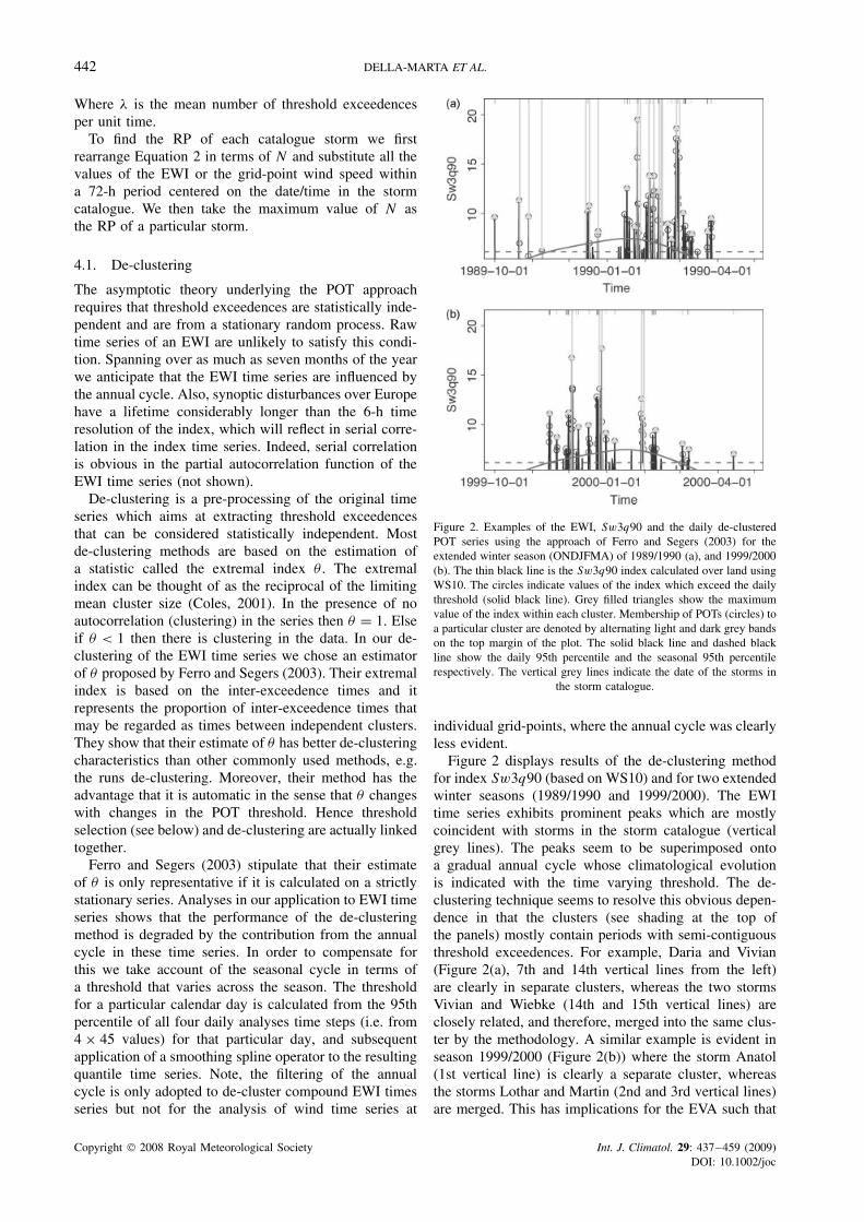
Figure 2. Examples of the EWI, Sw3q90 and the daily de-clusteredPOT series using the approach of Ferro and Segers (2003) for theextended winter season (ONDJFMA) of 1989/1990 (a), and 1999/2000(b). The thin black line is the Sw3q90 index calculated over land usingWS10. The circles indicate values of the index which exceed the dailythreshold (solid black line). Grey filled triangles show the maximumvalue of the index within each cluster. Membership of POTs (circles) toa particular cluster are denoted by alternating light and dark grey bandson the top margin of the plot. The solid black line and dashed blackline show the daily 95th percentile and the seasonal 95th percentilerespectively. The vertical grey lines indicate the date of the storms in

the storm catalogue.

individual grid-points, where the annual cycle was clearlyless evident.

Figure 2 displays results of the de-clustering methodfor index Sw3q90 (based on WS10) and for two extendedwinter seasons (1989/1990 and 1999/2000). The EWItime series exhibits prominent peaks which are mostlycoincident with storms in the storm catalogue (verticalgrey lines). The peaks seem to be superimposed ontoa gradual annual cycle whose climatological evolutionis indicated with the time varying threshold. The de-clustering technique seems to resolve this obvious depen-dence in that the clusters (see shading at the top ofthe panels) mostly contain periods with semi-contiguousthreshold exceedences. For example, Daria and Vivian(Figure 2(a), 7th and 14th vertical lines from the left)are clearly in separate clusters, whereas the two stormsVivian and Wiebke (14th and 15th vertical lines) areclosely related, and therefore, merged into the same clus-ter by the methodology. A similar example is evident inseason 1999/2000 (Figure 2(b)) where the storm Anatol(1st vertical line) is clearly a separate cluster, whereasthe storms Lothar and Martin (2nd and 3rd vertical lines)are merged. This has implications for the EVA such that



only the maximum wind within a cluster (grey trian-gles, Figure 2) is used in the GPD model. Hence inthis case the storms Lothar and Martin are treated asone storm. Note, that similar difficulties are encounteredfor storms in the catalogue when the corresponding EWIvalue is so low as to not exceed the threshold. A moredetailed comparison between the Ferro and Segers (2003)de-clustering and the classical runs de-clustering (notshown) reveals that there is little sensitivity on the RPresults to these two de-clustering methods (Della-Martaet al., 2007).

Figure 3 depicts similar de-clustering results calculatedfrom wind time series at two individual grid-points(a) north of the British Isles, (b) northeast of Europe.Extreme value analyses for individual grid-points is usedfor comparative purposes and for representativity tests(see later Section 5). The time series of WS10 show lessserial correlation than the index time series. Cataloguestorms tend to coincide with wind peaks (as is the casewith the EWI, Figure 2), but there is obviously muchweaker correspondence due to the more local characterof time series at grid-points.

4.2. Threshold choice

The threshold of the POT analysis should be largeenough to ensure near-asymptotic behaviour of the excee-dences. There are several diagnostic means to estimatea suitable threshold. These diagnostics build upon theknown threshold dependence of GPD parameters in theasymptotic tail (Coles, 2001). In this study, we have

Figure 3. As for Figure 2 but for the grid-points 2.5 °W, 57.5 °N (a),and 30 °E, 67.5 °N (b). Note that the EVA was performed on raw wind

values (units of ms –1) at each grid-point.

510

15

Mod

ified

Sca

le

642

631

596

533

424

320

208

136 80 51 35

–0.8

–0.4

0.0

Sha

pe

642

631

596

533

424

320

208

136 80 51 35

(a)

(b)

0

10 12 14

Threshold

2 4 6 8

10 12 14

Threshold

2 4 6 8

Figure 4. Modified Scale, σ∗ (see Coles, 2001) (a) and the shapeparameter, ξ , (b) diagnostic plots for selecting the fixed threshold NDUsabove which the de-clustered POT are modelled using the GPD. Thisexample is based on the de-clustered POT Sw3q90, WS10 using theland-only region. The vertical black lines denote the 95% confidenceintervals calculated using the parametric resampling technique detailedin Section 4.3. The numbers aligned vertically in the top of the plot arethe number of cluster maxima identified by the de-clustering technique.The lowest threshold value shown in each plot is the seasonal 70th

percentile, and the vertical grey line is the 95% quantile threshold.

inspected the asymptotic independence of the GPD shapeparameter and modified scale parameter upon threshold(Coles, 2001, chapter 4). These diagnostics are depictedin Figure 4 for index Sw3q90 (based on WS10). Forthreshold values smaller than about 6 NDUs there isclear dependence of the parameters on the threshold,but at larger values the variations are mostly containedwithin the uncertainty ranges of individual estimates.For the index under consideration a value of 6 cor-responds approximately to the 95th percentile (verti-cal grey line). Note that we have constrained theseresults by the choice of daily quantile used to de-cluster the time series (see above), and hence, thede-clustering and threshold selection are not indepen-dent of each other. Inspection of similar diagnostics forother indices reveals that the 95th percentile is a gen-erally acceptable choice of threshold. Based on theseresults, we have chosen the pertinent 95th percentileas the threshold for all indices. Clearly, there is nofinal proof that a particular choice is sufficient, sincethe assessment is also limited by sampling uncertainty.Some additional confirmation is, however, available fromquantile-quantile plots (see example in Figure 5), whichdemonstrates a good fit of the theoretical distribution



to the data. Additional checks are given in Della-Martaet al. (2007).

Threshold diagnostics for time series of wind at indi-vidual grid-points also show that a threshold correspond-ing to the 95th percentile is acceptable, i.e. asymptoticbehaviour was assured only beyond that value. Figure 6depicts the diagnostics for WS10 at one example grid-point. A value of 15.8 ms−1 corresponds to the 95thpercentile. Consideration of several grid-points suggestedthis quantile as a reasonable setting for the POT analysisat individual grid-points. For the de-clustering, however,we kept the seasonally varying threshold at the 90thpercentile which insured that only grid-points with anexceptionally strong seasonal cycle included a seasonallyvarying threshold.

10 15 20

1015

20

Model

Em

piric

al

Figure 5. A quantile-quantile (qq) plot (NDU) of the fitted GPD to thede-clustered POT Sw3q90, WS10 for the land-only region.

Mod

ified

Sca

le

–0.6

–0.4

–0.2

0.0

Sha

pe

(a)

(b)

510

150

Threshold

2012 14 16 18

2012 14 16 18

Threshold

1187

1172

1133

1048 88

9

647

430

281

170 95 48

1187

1172

1133

1048 88

9

647

430

281

170 95 48

Figure 6. As for Figure 4 but for the declustered POT WS10 grid-point2.5 °W, 57 °N.

4.3. Sampling uncertainty

Results from EVA can be subject to considerable sam-pling uncertainty. Classical procedures for estimating theuncertainty of GPD parameters (and related quantities,such as the RPs) encompass the asymptotic maximumlikelihood confidence intervals (also termed the deltamethod, see Coles, 2001), and resampling techniques. Thelatter builds on repeated estimates with random drawsfrom the dataset (non-parametric) or with random drawsfrom the best estimate distribution (parametric). Boththese techniques turned out to have limitations in ourapplication (see comparison below).

In the present study, we calculate confidence intervalsof RP estimates using the profile likelihood method.Profile likelihood confidence intervals are based on alikelihood ratio test. In practise, they are calculatedfrom a projection of the likelihood surface on therespective parameter axis, which can be obtained from asequence of numerical optimizations (Coles, 2001). Thelikelihood profile method is related to the delta methodbut exploits the true shape of the likelihood surfaceinstead of approximating it around its maximum. As aconsequence, calculating confidence intervals with thelikelihood profile methods makes more efficient use ofthe data points in the sample.

A comparison of results from all three techniques isdepicted in Figure 7 for index Sw3q90 (based on WS10).The figure shows the RL as a function of RP withpertinent confidence intervals from all three methods. Thecurvature of the best estimate (middle thick line) suggeststhat this index (like most others in this paper) exhibitsa short tail behaviour and hence its distribution functionhas an upper bound. The best estimate of the upper boundis around 90 NDU, but there is considerable uncertaintyabout its value. According to the delta method (dash-dotted line) and the parametric resampling (dashed line)there is non-zero probability that the upper bound is 84

Return Period (years)

Sw

3q90

0.5 10 20 50 100 200

5060

7080

521

Figure 7. A RL / RP plot showing the GPD fit (centre solidblack line) and a comparison of 95% confidence intervals usingthe methods outlined in Section 4.3. The index shown here is theSw3q90, WS10 using all grid-points. Horizontal axis: RP (years),vertical axis: RL (NDU). Different estimations of confidence intervals:profile log-likelihood (solid black), parametric resampling (dashedblack) and the delta method (dot dashed black). Note the log scale

on the horizontal axis.



NDU or lower (the lines for the lower confidence boundlevel off around this value). This is in contradiction withthe actual dataset, which comprizes events with indexvalues larger than 88 NDU. Obviously the upper bound ofthe distribution is necessarily larger than the largest datavalue. This is not reflected in the confidence intervalsof the delta method and the resampling. Both thesemethods do not take explicitly into account the highestdata values in the sample. In contrast, the confidencebounds calculated from the likelihood profile reveals anuncertainty range for the RLs which is shifted to largervalues and is consistent with the data at large RPs. Somemore general comparisons show that the likelihood profilemethod differs from the two other methods particularlyin cases with a short (bounded) tail. Consideration of thetrue likelihood surface in the profile method makes moredirect use of the data sample in estimating the samplinguncertainty and this avoids inconsistencies of confidenceintervals with the actual sample.

Short tail behaviour was observed with most of theEWI considered in this paper. We therefore chose thelikelihood profile method for estimating the samplinguncertainty of RPs (and distribution parameters). A slightmodification was however applied for RPs near thethreshold (typically for periods smaller than 0.2 years).For these cases, the likelihood profile was replaced bythe uncertainty in the mean exceedence based on theunderlying Poisson process.

5. Results

The Results Section is divided into three subsections.Firstly, the distributed (grid-point) and generalized (EWI)storm climatologies are presented in order to identifytheir similarities and differences. The second subsectionis devoted to comparing the RPs of wind storms derivedfrom the two different approaches answering researchquestions numbers two and three (Section 1). The finalsubsection is aimed at answering research question fouron the representativity of the generalized storm RPs forestimating the grid-point storm RPs.

5.1. Distributed and generalized storm climatologies

We fitted a GPD distribution to each of the 10 857grid-points over the domain to form an extreme windclimatology to be representative of the local extremewind climatology. As described in Section 4.2 we usedthe same fixed threshold (95% quantile) in the grid-point GPD model as the EWI (95% quantile), based onthe extensive diagnostic checks performed for individualgrid-points. Generally, the GPD fits to POT series atindividual grid-points, (assessed using qq-plots) is verygood (not shown). We quantified this more rigorouslyusing an Anderson-Darling (A2) goodness-of-fit test(Choulakian and Stephens, 2001) and find that 74% of thefitted GPDs passed this test at the 5% significance level.

Figure 8 provides a summary of the important param-eters of the EVA at each grid-point. Figure 8(a) shows

the empirically based seasonal 95% quantile threshold(u) of WS10. Generally, there are higher winds over theNorth Atlantic Ocean and the British Isles than over thenorth, east and south of the domain. The average numberof extreme wind events per season, λ shows a band oflower values running from the southwest of the domain tothe northeast of the domain, whereas in the northwest, thesoutheast as well as the far northeast there are higher val-ues of λ (Figure 8(b)) corresponding to the major stormtrack and genesis areas of the Northeast Atlantic and theMediterranean regions respectively. Values of λ rangefrom approximately 6 to 25. The spatial distribution ofσ , the scale parameter of the GPD (Equation 1), resem-bles the distribution of u, i.e. a wider GPD distributionover ocean areas compared to land areas (see Monahan,2004, for a physical explanation). The shape parameterξ is rather mixed and shows little spatial coherency. Insome cases, individual grid-points have a slightly posi-tive shape parameter indicating that the GPD has no upperlimit. The extremal index θ (Section 4.1), a measure ofthe tendency for storms to cluster in time, is almost identi-cal in appearance to the spatial distribution of λ. θ showsa wide area of the domain east of the main North Atlanticstorm track where θ is lower than around 0.3 indicatingthat extreme wind events tend to form larger clusters thatare separated by more time in this region compared to thewestern North Atlantic, south of the Alps and the easternMediterranean, in part confirming the storms clusteringanalysis of Mailier et al. (2006) for cyclone count-basedstatistics. This process is evident in Figure 3 which showsthe de-clustered POT series for two points, one wherethere is clearly more clustering (Figure 3(a), higher λ andlower θ ) and the other where there is less clustering ofextreme winds (Figure 3(b), lower λ and higher θ ). TheRL for various RPs are shown in Figure 9. Note that thepurpose of this figure is to compare the relative differ-ences in the RLs for various RPs and not as a measureof the absolute magnitude of surface wind speeds. Foreach of the RPs a similar spatial structure of the extremewinds can be seen, with higher values in the far westof the domain and over ocean regions than over land.Relatively high values can be seen over the British Islesand the north coast of Spain as well as the western andnorthern coasts of western Europe with relatively lowervalues over Scandinavia, eastern and southern Europe.

The generalized wind-storm climatology is presentedas a RL/RP plot in Figures 10 and 11. The RL/RPplot summarizes the fitted GPD (i.e. the extreme windclimatology) together with the estimates of the RP andRL of each of the catalogue wind storms which are abovethe chosen threshold. Using the Sw3q90 index calculatedfrom WS10 over the whole domain we estimate awide range of RPs (Figure 10, vertical grey lines) forthe catalogue storms between approximately 0.2 and18 years. These estimates are based on the GPD fit(black line) and not the cluster maxima (black dots).The curvature of the GPD fit is negative, indicating thatthe shape parameter is negative (ξ , Equation 2) and thatthere is a physical upper limit to the extreme process.



Figure 8. Parameters of the grid-point EVA (Section 4) for WS10. (a) The grid-point empirical 95% quantile threshold, u (ms−1) and the MLEsof the GPD fit (Equations 1 and 2) , (b) the average number of extreme wind events per season after de-clustering, λ, (c) the scale parameterof the GPD, σ , (d) the shape parameter of the GPD, ξ , and the extremal index, θ (Section 4.1) (e). This figure is available in colour online at

www.interscience.wiley.com/ijoc

This is in agreement with distributed storm climatology(see Figure 8(d)). Figure 11 shows the generalized stormclimatologies of all five indices calculated using land-only grid-points. The climatologies all exhibit a negativeshape parameter in the range −0.23 ≤ ξ ≤ −0.10 andeach have a similar number of storm occurrences perseason, λ in the range of 8.2 ≤ λ ≤ 11.0. The scaleparameter varies greatly due to the different units of eachEWI. The quality of the GPD fit to each of the EWI wasassessed using qq-plots (e.g. Figure 4) and the Anderson-Darling (A2) test. The quality of the fit assessed using thisstatistic was noticeably the best for the index Sw3q90 andthe worst for the index Q95. Comparing Figure 11 withFigure 10 it is noticeable that there is a greater range ofRP estimates for the catalogue storms. This reflects thatthe sampling of wind storms in the catalogue is biasedtowards wind storms which had an impact on the western

European region. With this in mind, and returning toFigure 10, we see that there are a number of storms inthe EWI (black dots) that do not coincide with the sevenmost extreme catalogue storms (grey lines). A sign thatmore intense wind storms have occurred in the northeastNorth Atlantic than documented in the storm catalogue.

5.2. Distributed and generalized return periodsfor prominent European wind storms

In this section, we present a comparison of the RPs ofcatalogue wind storms using the generalized and dis-tributed wind storm climatologies highlighting the majorsources of uncertainty. We start with an intercompari-son of the EWIs using either WS10 or FG10. Figure 12presents scatter-plots of the catalogue storm RPs esti-mated using FG10 versus the RPs using WS10 for eachindex for the land-only domain. On each plot there are



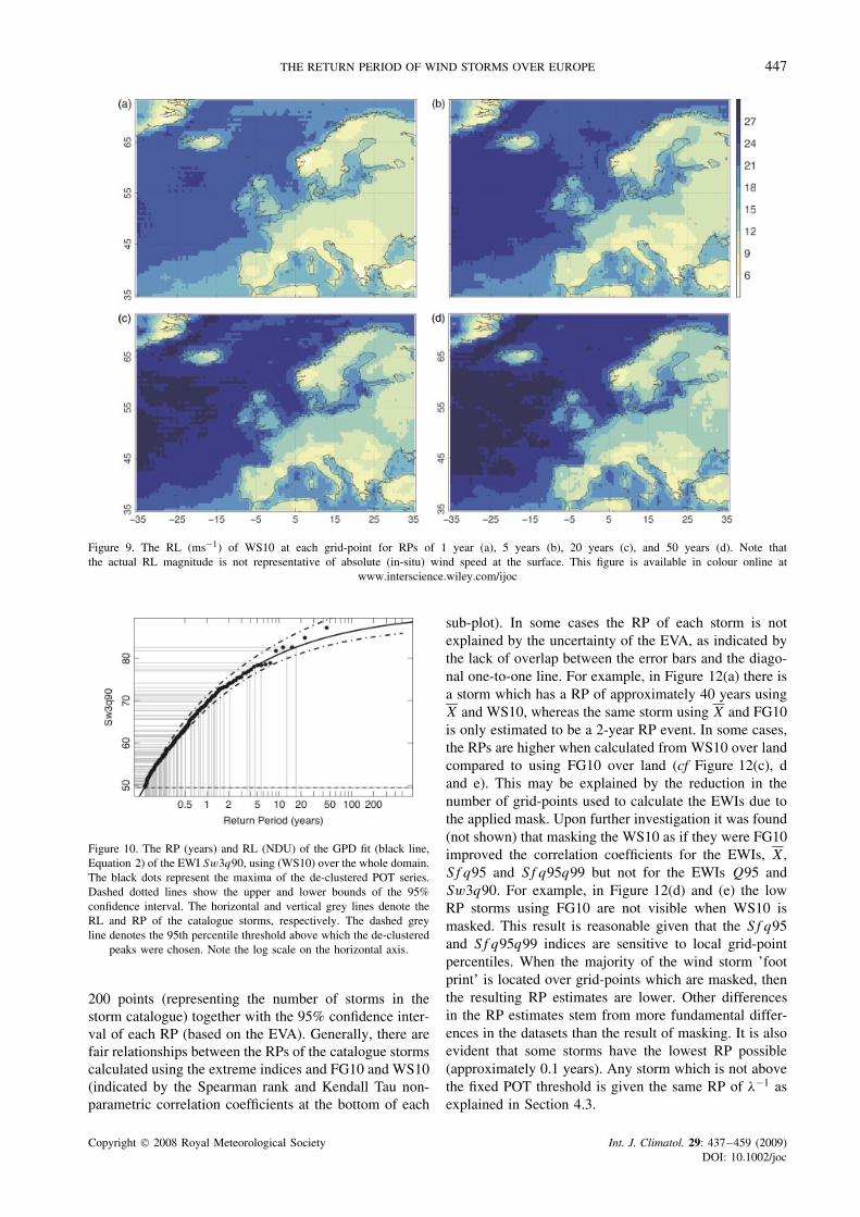
Figure 9. The RL (ms−1) of WS10 at each grid-point for RPs of 1 year (a), 5 years (b), 20 years (c), and 50 years (d). Note thatthe actual RL magnitude is not representative of absolute (in-situ) wind speed at the surface. This figure is available in colour online at


Figure 10. The RP (years) and RL (NDU) of the GPD fit (black line,Equation 2) of the EWI Sw3q90, using (WS10) over the whole domain.The black dots represent the maxima of the de-clustered POT series.Dashed dotted lines show the upper and lower bounds of the 95%confidence interval. The horizontal and vertical grey lines denote theRL and RP of the catalogue storms, respectively. The dashed greyline denotes the 95th percentile threshold above which the de-clustered

peaks were chosen. Note the log scale on the horizontal axis.

200 points (representing the number of storms in thestorm catalogue) together with the 95% confidence inter-val of each RP (based on the EVA). Generally, there arefair relationships between the RPs of the catalogue stormscalculated using the extreme indices and FG10 and WS10(indicated by the Spearman rank and Kendall Tau non-parametric correlation coefficients at the bottom of each

sub-plot). In some cases the RP of each storm is notexplained by the uncertainty of the EVA, as indicated bythe lack of overlap between the error bars and the diago-nal one-to-one line. For example, in Figure 12(a) there isa storm which has a RP of approximately 40 years usingX and WS10, whereas the same storm using X and FG10is only estimated to be a 2-year RP event. In some cases,the RPs are higher when calculated from WS10 over landcompared to using FG10 over land (cf Figure 12(c), dand e). This may be explained by the reduction in thenumber of grid-points used to calculate the EWIs due tothe applied mask. Upon further investigation it was found(not shown) that masking the WS10 as if they were FG10improved the correlation coefficients for the EWIs, X,Sf q95 and Sf q95q99 but not for the EWIs Q95 andSw3q90. For example, in Figure 12(d) and (e) the lowRP storms using FG10 are not visible when WS10 ismasked. This result is reasonable given that the Sf q95and Sf q95q99 indices are sensitive to local grid-pointpercentiles. When the majority of the wind storm ’footprint’ is located over grid-points which are masked, thenthe resulting RP estimates are lower. Other differencesin the RP estimates stem from more fundamental differ-ences in the datasets than the result of masking. It is alsoevident that some storms have the lowest RP possible(approximately 0.1 years). Any storm which is not abovethe fixed POT threshold is given the same RP of λ−1 asexplained in Section 4.3.



Figure 11. As for Figure 10, but the RP (years) and RL of the GPD fit (black line, Eqn. 2) of the EWI (a) X, (b) Q95, (c) Sw3q90, (d) Sf q95,and (e) Sf q95q99 using WS10 over the land domain.

An intercomparison of catalogue storm RPs fromdifferent EWIs shows that with some EWI, data andmask combinations result in very similar RP estimates (interms of rank correlations, not shown), while others arevery different from one another. Inter-index comparisonsindicate that X, Sf q95 and Sf q95q99 are most highlycorrelated with each other for both datasets (FG10 andWS10) and for all masks. Whereas, correlations betweenRPs of Sw3q90 and X or Sf q95 or Sf q95q99 arelowest contrasting the differences in the sensitivitiesof these indices. Inter-dataset indices all show similarcorrelations (cf Figure 12). Note that the range of inter-index correlations (0.49 < Spearman rank correlations <

0.94) is larger than the range of inter-dataset correlations(0.84 < Spearman rank correlations < 0.89), indicating

that greater differences between RP estimates are dueto the EWIs rather than the datasets. Some plausibleexplanation for these differences are presented later inSection 5.3 and is related to the sensitivity of the EWIsto the domain and storm catalogue.

Figure B-1 presents an overview of RPs of promi-nent wind storms from the storm catalogue calculatedusing WS10 (a) and FG10 (b). It has been placed inAppendix B since we envisage that it could be used as areference for readers who wish to see individual storm RPestimates (which are not possible to derive from previousfigures). For each storm above the threshold, the name(when known) and date, as well as the 95% confidenceinterval of the storm RP is shown using the EWI Sw3q90(other EWIs are available upon request). The number of



WS10 Return period (years)SpearmanCor: 0.86 / KendallTauCor: 0.69


(a) (b)

(c) (d)

(e)

FG

10 R

etur

n pe

riod

(yea

rs)

0.5

110

2050

100

25


0.5 1 10 20 50 1002 5

FG

10 R

etur

n pe

riod

(yea

rs)

0.5

110

2050

100

25


0.5 1 10 20 50 1002 5

0.5 1 10 20 50 1002 5

FG

10 R

etur

n pe

riod

(yea

rs)

0.5

110

2050

100

25


0.5 1 10 20 50 1002 5

0.5 1 10 20 50 1002 5

0.5

110

2050

100

25

0.5

110

2050

100

25

FG

10 R

etur

n pe

riod

(yea

rs)

FG

10 R

etur

n pe

riod

(yea

rs)

Figure 12. Comparison of RP (years) over land for the 200 catalogue wind storms calculated using FG10 and WS10 for each of the five EWI, (a)X, (b) Q95, (c) Sw3q90, (d) Sf q95, and (e) Sf q95q99. Note the logarithmic scale. 95% confidence intervals for each of the RPs are denotedby the vertical (FG10) and horizontal (WS10) whiskers on each point. At the bottom of each sub-figure is the Spearman rank and Kendall Tau

correlation coefficient.

catalogue storms above the 95th percentile threshold ofthe index Sw3q90 is 158 and 161 storms respectively.However, only the common storms above each thresholdrespectivley are shown for comparison purposes (153).Generally, the range of RP estimates is similar usingeither FG10 or WS10, and the RPs of individual stormsare quite consistent with one another. In summary, theEWIs summarize the extreme wind climatology over adomain and offer a single estimate of the extreme windRP of a storm which may be intuitively appealing for

applications, such as in the reinsurance industry where asingle estimate of the intensity of an event is needed toexplain an aggregated loss over a portfolio. The EWIs area spatial summary statistic, and hence, the RPs estimatesare representative of the RP of a storm, that could haveoccurred anywhere over the chosen domain.

Similarly as for the EWIs, we investigated the effect ofusing different data to estimate the RP of the cataloguestorms at the grid-point level (distributed view). Wefound that achieving a consistent estimate of RP for each



of the catalogue storms at individual grid-points is asdifficult as when using different EWIs and datasets. Apossible reason for the lack of correspondence betweenthese estimates is due to fundamental differences in FG10and WS10. Figure 13 presents the spatial distribution ofRPs of FG10 and WS10 associated with selected stormsin the 1989/1990 and 1999/2000 seasons. Qualitativelythe fields in Figure 13 are similar, but however, on aregional and grid-point level the differences are greater,especially for the storm Lothar (Figure 13(e) and (f)).Lothar was a very fast moving mesoscale cyclone and itsRP estimates are aliased due to the sampling frequency ofWS10 shown as ‘islands’ of higher RP winds. Recall thatthe 6-hourly values of FG10 represent the maximum windgust during a 6-h period, whereas the 6-hourly values

of WS10 are the instantaneous analysis values. Anotherpoint to keep in mind when interpreting this figure is thatthe individual grid-point RPs are not the instantaneousRPs at the date and time of the storm, but the maximumRP calculated using the 72-h maximum FG10 and WS10centred on the storm date/time. This was done in order toensure that we capture the RP of the storm and not justthe RP at the time of analysis. The RP patterns for Vivian(Figure 13(a) and (b)) are qualitatively similar, however,the area of maximum grid-point RPs using FG10 is largerthan with the corresponding WS10 analysis. Possiblereasons for these discrepancies could be storm-specificdynamics (Wernli et al., 2002; Holton, 2004) which pro-duced stronger gust speeds (and hence higher RPs) thanare usually associated with the corresponding WS10, or

Figure 13. The RP (years) for each grid-point for the selected catalogue storms in the 1989/1990 and 1999/2000 October–April extended winterseasons estimated from FG10 and WS10, (a) Vivian: 26 Feb 1990 1200UTC, using FG10, and (b) using WS10, (c) Anatol: 3 Dec 1999 1200UTCusing FG10, and (d) using WS10, (e) Lothar: 26 Dec 1999 0000UTC using FG10, and (f) using WS10. The RP scale is in the top right of theplot. Note that grey areas in (a), (c) and (e) denote masked values. This figure is available in colour online at www.interscience.wiley.com/ijoc



remaining problems in the ERA-40 gust parameteriza-tion scheme. Storm-specific dynamics are likely to bethe reason for this discrepancy since an investigation ofthe PartnerRe high-resolution wind gust field reveals (notshown) a qualitatively similar pattern to the RPs shownin Figure 13(a). In the other example shown, the stormAnatol has a very similar structure and magnitude ofRPs (Figure 13(c) and (d)) using either FG10 or WS10.Another limitation of using WS10 (Figure 13(b) and (f))is the lack of high RPs over the Alps. This could be dueto the climatologically low wind speeds (see Figure 8(a)and Figure 9) at 10 m perhaps caused by problems inthe parameterization of wind speed in areas of complexorography. It is clear from other examples (not shown)that the estimation of RPs of storms that are less than 72h apart from each other are either very similar or verydisparate (e.g. Lothar and Martin, separated by approxi-mately 48 h) due to the criteria of taking the maximumgrid-point wind RP over a 72-h period.

A qualitative comparison of RPs calculated from thegeneralized EWIs and the distributed grid-point approachdemonstrates their utility in estimating the RPs of cat-alogue storms during the 1989/1990 and 1999/2000extended winter seasons. Tables 1 and 2 summarize theRPs calculated using Sw3q90 and WS10 or FG10 overland and the range of grid-point RPs over land, respec-tively. The most severe wind storm in these two seasons(according to this index and dataset, Table 1), is associ-ated with the storm Daria, with an RP estimated to be24.1 years (see also Figure 14(b)). Its corresponding RPestimates using the same index, but FG10, is approxi-mately 39 years (Table 2), and although these estimatesdiffer they are well contained within each of the uncer-tainty estimates. In the grid-point analysis the same stormhas produced local winds over land to be between 0.1 and200+ years (see Figure 14(b)) with some of the individ-ual grid-point RPs as high as 1500 years in the EnglishChannel area, where the storm had its highest intensity.By comparing the value of the third quartile of grid-pointRPs with the Sw3q90 RPs for all storms and both datasets(Tables 1 and 2), we can say that the EWI RP and thegrid-point RPs are in qualitative rank-order agreementfor most storms. The major exception to this rule is forthe storm Vivian, where the EWI RP estimates differgreatly between datasets (13.1 years using WS10, and 374years using FG10) but do not differ greatly comparing thethird quartile of grid-point RPs (10.6 years usingWS10and 9.4 years using FG10). However, this result is notunreasonable given the large uncertainty in the EWI RPestimates and individual differences in storm dynamicsrepresented by FG10 and WS10 as stated above. It isinteresting to note that when using Sf q95 the six leastfrequent storms are all unnamed storms and different tothose derived from Sw3q90 contrasting the differencesbetween these indices. If we look in more detail to thestorms Lothar and Martin we can see that the RP esti-mates differ substantially between datasets due to boththe mask applied to FG10 and the aliasing of the sig-nal due to WS10. While the grid-point RP analysis also

Figure 14. As for Figure 13 but the RP (years) of WS10 for eachgrid-point estimated for the storm Daria: 26 Jan 1990 0000UTC (b). In(a) and (c) are shown the upper (lower) bound of the 95% confidenceinterval of the RP (years). This figure is available in colour online at


exhibits dependence on the dataset at the grid-point level,qualitatively the pattern and magnitude of the RPs aresimilar (see Figure 13(a)–(d)). The RPs for storm Lotharover Switzerland (Figure 13(e) and (f)) are hard to com-pare with Albisser et al. (2001) due to the masking andaliasing effects of the ERA-40 data used here.

5.3. Representativity of continental RPs

A basic evaluation of the ability of the EWI RP esti-mates to represent the grid-point wind-based RP esti-mates for the 200 wind storms has been performed usinga Spearman rank (and Kendall Tau) correlation analy-sis. Figure 15 demonstrates that the rank of the RPs ofSw3q90 are most highly correlated with the rank of theRPs from the grid-point analysis over a region centredin the mid-western part of the domain over the NorthAtlantic Ocean (Figure 15(a)) with r values in the order



Figure 15. The Spearman rank correlation between the RPs of the 200 catalogue storms based on Sw3q90 of WS10 and the RP at each grid-pointbased on WS10, (a) using all grid-points, and (b) land grid-points only.

of 0.4–0.6. The rank correlation decreases radially fromthis point such that r over the European coast and furtherinland is between 0 and 0.3 implying that these indicesonly share a small fraction of variability of the localgrid-point RPs. Results are better if we consider EWIusing land grid-points (Figure 15(b)). Here, again we seea ’bullseye’ centred on western central Europe. Withinthese regions, r ranges from 0 to 0.7 indicating that a rea-sonable amount of shared variability exists between grid-point RPs and the EWI RPs. For the other indices (exceptQ95) it is important to note that the centre of highest r

over the land-only domain is located further east (eastof Germany, not shown). This may explain why Sw3q90and Q95 have a higher number of catalogue storms abovethe 95% quantile threshold (161 and 152, respectively)than the other EWI (145, 137 and 143 for X, Sf q95 andSf q95q99, respectively) since the region of highest sen-sitivity of the index also coincides with the region overwhich most of the catalogue storms have been selected.

6. Conclusions and discussion

We use state-of-the-art reanalysis data combined withextreme value analysis techniques to estimate the clima-tology of extreme winds and the recurrence frequencyof prominent wind storm events over Europe during theperiod from 1957 to 2002. If we return to the originalaims of the study which are reiterated below, we concludethe following from this analysis:

How reliable are wind parameters in the ERA-40reanalysis (spatial representativity, temporal homogene-ity) for estimating RPs of high-impact storm events overEurope?

• FG10 from ERA-40 should not be used in areas wherethe roughness length parameter is high (>3m), dueto the boundary-layer physics in the ERA-40 model.Such areas should be masked from the analysis (cfFigure 1).WS10 from ERA-40 appears to be free fromthe problems associated with high wind gust values,however, 10-m winds over complex orography mightto be too low (cf Figure 8(a) and Figure 9).

• WS10 (and any other analysed wind-speed parameters)represents the instantaneous wind speed at the reanal-ysis output time which results in aliasing of the windspeed and hence contributes to the unreliability of RPsin both the generalized and distributed approaches toRP estimation. FG10 represents the maximum windgust during the previous 6 h and does not suffer fromthis problem.

• Both the generalized and distributed extreme windclimatologies demonstrate the expected land–sea con-trasts and a negative shape parameter of the GPD.

• The distributed wind storm climatology shows anincreased storm frequency and decreased storm clus-tering in the Northeast Atlantic associated with thestorm track, and the Mediterranean region of secondarycyclogenesis confirming the results of Mailier et al.(2006) (cf Figure 8(e)).

How sensitive are estimates of RPs to the details in thedefinition of the EWIs?

• The EWIs X, Sf q95 and Sf q95q99 result in similarRP estimates for individual storms. These indicesshould be used when more weight to local windsrelative to their climatology is needed, and to findstorms also affecting regions not subject to regularextreme wind events.

• The EWIs Sw3q90 and Q95 result in similar RPestimates for individual storms. These indices shouldbe used when more weight to the absolute magnitudeof a wind storm is needed, regardless of the local windclimatology.

• The RPs estimates from Sw3q90 and Q95 are morerepresentative of loss figures published in MunichRe(2000) than the remaining EWIs. We note that thequality of the GPD fit to Q95 shown in Figure 11(b)is lower than other indices.

• EWI storm RPs are most sensitive to the domainover which they are calculated, and to a lesser extent,the definition of the index. Higher RPs result fromusing land-only grid-points than from using the wholedomain. This is partly due to the storm catalogue beingbiased towards wind storms which had an impact on



continental Europe, especially in the northwest, anddue to the process of spatial averaging.

What is the degree of uncertainty in estimatingcontinental-scale and grid-point-scale RPs for paststorms? Which factors contribute most to the uncertainty?

• The largest uncertainties in RP estimates (both thegeneralized and distributed approaches) derive fromthe differences in the wind gust and wind-speed data(such as masking and aliasing, mentioned above)generally for RPs less than 10 years. This uncertaintytends to be comparable with the uncertainty associatedwith the GPD fit at higher RPs (cf Figure 12, Tables 1and 2).

• The RPs calculated using either Sw3q90 or Q95compared with either X, Sf q95 or Sf q95q99 showsthat the EWI definition plays a greater role in the RPdifferences than the wind parameter chosen.

• The spatial distribution of RPs for catalogue storms isgenerally similar using either WS10 or FG10. Physicalprocesses leading to extremes specific to individualstorms may not be adequately captured by WS10 andhence the calculation of RPs.

• The method of taking the maximum RP within a 72-hperiod prevents an accurate RP estimate for cataloguestorms which occurred less than 72 h apart from oneanother. This aspect of the data processing preventsthe estimates of RPs from storms such as Lotharand Martin from being independent. This method alsopotentially biases RPs to the time when the storm hasits maximum intensity, and not necessarily at its peakimpact.

• In some cases, the catalogue storm dates/times do notmatch the cluster maxima of the EWI or the grid-pointwind exactly. This could be due to the fact that thecatalogue storm dates were recorded when the stormhad the highest impacts, and not necessarily when thestorm had its highest intensity.

How representative are continental-scale estimates ofRPs as a measure of the local recurrence of a storm?

• The generalized and distributed RP estimates shareup to approximately 50% of common variations. Thelarger the domain considered the lower the effective-ness of the EWI at explaining local wind RPs. TheSw3q90 and Q95 indices have the highest correla-tions with local RP estimates due to these indicesbeing based on an absolute wind-speed magnitude.Best correlations coincide with regions of climatologi-cally highest magnitude winds (over land, cf Figure 9).The success of these indices is also partly due tothe way in which the storm catalogue was created.The storm catalogue is biased towards storms whichoccurred in the region of interest of the source docu-ments, which in this case, is mainly focused on north-western Europe.

We can also state various conclusions associated withthe chosen EVA methodologies: The generalized Paretodistribution is a robust extreme-value model of the de-clustered peak over threshold (POT) series obtainedfrom EWI and grid-point wind speed. The POT serieswas obtained using an automatic de-clustering methodwhich largely avoided the need for the specification ofarbitrary parameters as is the case with more commonde-clustering methods. To determine the uncertainty ofthe extreme wind climatology and catalogue storm RPs,the profile log-likelihood method is used as it givesmore physically meaningful results than other commonmethods. The choice of de-clustering method (either theFerro and Segers (2003) or runs-de-clustering (Coles,2001), not shown, see Della-Marta et al., 2007), has littleeffect on RPs of catalogue storms calculated using EWIs,however, the quality of the GPD fit can be affecteddepending on whether the seasonal cycle of the indexis included in the de-clustering.

The question of determining the RP of a ’windstorm’ is rather ill-posed since a wind storm has manydegrees of freedom which are difficult to summarize ina generalized or a distributed approach. The EWIs area spatial summary statistic, and hence, the estimates ofRPs are more representative of the RP of a storm thatcould have occurred anywhere over the chosen domain.We conclude that it is very difficult to obtain a spatialsummary statistic (EWI) which works equally well foreach type of storm event in the context of trying toestimate a storm RP, although Sw3q90 seems to havehigher representativity of the given catalogue storms thanthe other indices. On the other hand, the grid-point windspeed RPs also show dependency between datasets, andmay not be used to estimate the RP of the storm given thatno spatial dependence between grid-point RPs is takeninto account.

We did not include any treatment of non-stationarity inour GPD model since there is little evidence of any long-term linear trends in storminess over Europe during thepast 100 years (e.g. Alexandersson et al., 2000) however,there remains decadal variability in the dataset (e.g. themore frequent and higher-intensity storms in the 1990s)which does affect the interpretation of RPs such as thoselisted in Tables 1 and 2. For example, both Daria andVivian, two high-RP storms, occurred during the sameseason. Further analysis of the trends in the DPOT seriesof each EWI show (not shown) an increase (significant at0.05 level) over land areas using Sw3q90, whereas, noother index indicates a trend during this period.

As more accurate and longer datasets of either in-situ wind data, pressure datasets or dynamically down-scaled reanalyses become available (Diaz et al., 2002;Alexander et al., 2005; Ansell et al., 2006; Heneka et al.,2006; Schwierz et al., 2008) this analysis should berepeated in order to minimize the uncertainty in theRP calculations. We also recommend further researchinto the spatial structure of historical wind storm eventsthrough the application of advanced spatial EVA tech-niques (Coles, 2001). Given the lack of longer and more



Tabl

eI.

The

RPs

ofso

me

prom

inen

tw

ind

stor

ms

inth

est

orm

cata

logu

edu

ring

the

1989

/199

0an

d19

99/2

000

exte

nded

win

ter

seas

ones

timat

edus

ing

the

EW

ISw

3q90

base

don

WS1

0.

Stor

mN

ame

Dat

e/T

ime

Low

erR

PU

pper

Reg

ion

affe

cted

Gri

dPo

int

RP

rang

e

(Yea

rs)

(Yea

rs)

(Yea

rs)

Min

.1s

tQ

u.M

edia

n3r

dQ

u.M

ax.

unkn

own

17-1

2-19

8912

:00

0.31

0.36

0.40

GB

,E

S,PT

,IT

,SI

,H

R0.

10.

420.

711.

9820

0+D

aria

26-0

1-19

9000

:00

9.72

24.1

075

.80

GB

,FR

,B

E,

NL

,L

U,

DE

,D

K0.

10.

481.

285.

2820

0+H

erta

04-0

2-19

9000

:00

0.88

1.09

1.37

IE,

GB

,FR

,D

E0.

10.

460.

711.

4720

0+N

ana

12-0

2-19

9012

:00

0.49

0.58

0.69

ES,

FR,

IE,

GB

0.1

0.43

0.72

1.20

10.3

Viv

ian

26-0

2-19

9012

:00

6.46

13.1

029

.60

IE,

GB

,FR

,B

E,

NL

,L

U,

CH

,D

E,

DK

,SE

,PL

,LT

,LV

,E

E,

AT

,C

Z0.

10.

611.

8810

.60

200+

Wie

bke

01-0

3-19

9000

:00

3.64

5.97

10.1

0FR

,D

E,

AT

,C

Z,

CH

,IT

0.1

0.55

1.12

3.32

137.

0A

nato

l03

-12-

1999

12:0

02.

824.

316.

72G

B,

NL

,D

E,

DK

,PL

,LT

,B

Y0.

10.

480.

862.

4620

0+L

otha

r26

-12-

1999

00:0

00.

811.

001.

24G

B,

FR,

CH

,A

T0.

10.

410.

661.

3420

0+M

artin

28-1

2-19

9900

:00

4.30

7.45

13.5

0E

S,FR

,C

H,

AT

,IT

0.1

0.43

0.74

2.71

200+

Ker

stin

29-0

1-20

0012

:00

0.57

0.68

0.81

GB

,D

K,

SE,

FI0.

10.

410.

631.

0212

2.0

Col

umns

3an

d5

show

the

low

eran

dup

per

boun

dof

the

95%

confi

denc

ein

terv

alof

the

stor

mR

P(C

olum

n4)

.T

he‘R

egio

naf

fect

ed’

colu

mn

show

sth

eco

untr

ies

mos

taf

fect

edby

the

stor

ms

asse

ssed

usin

gth

egr

id-p

oint

RP

estim

ates

.T

heco

untr

yco

des

are

stan

dard

ISO

two-

lette

rco

des

(see

http

://w

ww

.iso.

org/

iso/

coun

try

code

s/).

Col

umns

9–

11gi

vean

impr

essi

onof

the

dist

ribu

tion

ofgr

id-p

oint

RPs

over

land

area

sw

ithin

the

dom

ain,

whe

reM

in.

isth

em

inim

umgr

id-p

oint

RP,

1st

(3rd

)Q

u.is

the

first

(thi

rd)

quar

tile,

Med

ian

isth

em

edia

n,an

dM

ax.

isth

em

axim

umgr

id-p

oint

RP

whe

reR

Psgr

eate

rth

an20

0ye

ars

are

repl

aced

by‘2

00+’

,si

nce

the

erro

ras

soci

ated

with

thes

eR

Pes

timat

esis

extr

emel

yla

rge.

Tabl

eII

.T

heR

Psof

som

epr

omin

ent

win

dst

orm

sin

the

stor

mca

talo

gue

duri

ngth

e19

89/1

990

and

1999

/200

0ex

tend

edw

inte

rse

ason

estim

ated

usin

gth

eE

WISw

3q90

base

don

FG10

.Se

eTa

b.1

capt

ion

for

mor

ede

tails

.

Stor

mN

ame

Dat

e/T

ime

Low

erR

PU

pper

Reg

ion

affe

cted

Gri

dPo

int

RP

rang

e

(Yea

rs)

(Yea

rs)

(Yea

rs)

Min

.1s

tQ

u.M

edia

n3r

dQ

u.M

ax.

unkn

own

17-1

2-19

8912

:00

0.42

0.49

0.57

GB

,E

S,PT

,IT

,SI

,H

R0.

10.

380.

711.

154.

73D

aria

26-0

1-19

9000

:00

13.9

039

.60

125.

00G

B,

FR,

BE

,N

L,

LU

,D

E,

DK

0.1

0.53

1.88

6.79

200+

Her

ta04

-02-

1990

00:0

00.

550.

650.

77IE

,G

B,

FR,

DE

0.1

0.40

0.60

0.90

3.20

Nan

a12

-02-

1990

12:0

00.

520.

620.

73E

S,FR

,IE

,G

B0.

10.

521.

132.

0410

.20

Viv

ian

26-0

2-19

9012

:00

45.0

037

4.00

4000

.00

IE,

GB

,FR

,B

E,

NL

,L

U,

CH

,D

E,

DK

,SE

,PL

,LT

,LV

,E

E,

AT

,C

Z0.

10.

881.

929.

4220

0+W

iebk

e01

-03-

1990

00:0

01.

061.

341.

72FR

,D

E,

AT

,C

Z,

CH

,IT

0.1

0.52

0.90

3.11

200+

Ana

tol

03-1

2-19

9912

:00

2.09

2.93

4.17

GB

,N

L,

DE

,D

K,

PL,

LT,

BY

0.1

0.52

1.28

4.52

200+

Lot

har

26-1

2-19

9900

:00

2.90

4.36

6.63

GB

,FR

,C

H,

AT

0.1

0.46

0.92

3.65

200+

Mar

tin28

-12-

1999

00:0

00.

650.

790.

96E

S,FR

,C

H,

AT

,IT

0.1

0.42

0.78

2.21

200+

Ker

stin

29-0

1-20

0012

:00

0.84

1.03

1.29

GB

,D

K,

SE,

FI0.

10.

460.

691.

1083

.80



reliable reanalysis or in-situ data, utilization of the ever-increasing amount of dynamical ensemble prediction data(van den Brink et al., 2004a,b; Jung et al., 2005; Freiet al., 2006) is suggested as a means to build more real-istic estimates of the frequency of wind storms.

In conclusion, the results demonstrate that significantprogress has been made through the development of anextreme wind climatology based on a robust reanalysisdataset consistent in space and time. We have created aclimatology of wind storm RPs based on EWIs togetherwith estimates of their local wind RP using the grid-pointapproach. Considerable challenges remain both from themethodological treatment of spatial extreme events andfrom the limitations imposed by the currently availabledatasets.

Acknowledgements

We wish to acknowledge PartnerRe who substantiallysponsored this research. We wish to thank Herve Castella,Malcolm Haylock, Manuel Prechtl from PartnerRe, andFelix Fundel from MeteoSwiss, for useful discussions andinputs to this paper. Malcolm Haylock suggested the for-mulation of the index Sw3q90. Two anonymous review-ers provided detailed comments and suggestions whichresulted in a substantially improved paper. Paul Della-Marta was partially funded by the 6th EU framework pro-gram ENSEMBLES contract number GOCE-CT-2003-505539, and by the Swiss National Science Foundationthrough the National Centre for Competence in ResearchClimate (NCCR-Climate) Sponsors: Reinsurance Com-pany, Zurich, Switzerland 6th EU framework programENSEMBLES contract number GOCE-CT-2003-505539Swiss National Science Foundation through the NationalCentre for Competence in Research Climate (NCCR-Climate).

Appendix A

This appendix describes each of the Extreme WindIndices (EWI) in mathematical notation for the benefitof readers who may wish to implement such indices.The indices are denoted in terms of a generic windvariable, W and could be substituted for either FG10 orWS10. Where possible, we tried to take into account theunequal areas of each grid box by weighting sums andmultipliers by the cosine of the latitude of each grid-point.A rationale for each index is given in Section 3.

X: Mean wind (units of ms−1).

X (t) = 1

Nκδ

∑x,y∈δκ(x, y)w(x, y, t) (A1)

where κ are the individual grid-point weights whichonly depend on y, κ (x, y) = cos (latitude (y)), Nκδ =∑

x,y∈δ κ (x, y) and δ denotes the domain.

Q95: The spatial 95% quantile wind (units of ms−1).

Q95(t) = F −1∗ (p) = min{w : p ≤ F∗(W)} (A2)

where p = 0.95 and F∗ is the latitude weighted empir-ical cumulative distribution function of {w(x, y, t) :(x, y) ∈ δ} where δ denotes the domain. The weightedcumulative distribution function is given by Horvitz andThompson, 1952; R Development Core Team, 2005).

F∗ (W) = 1

Nκδ

∑x,y∈δκ(x, y) (w(x, y, t) ≤ W) (A3)

Where κ are the individual grid-point weights and Nκδ is

given above and ={

1 : w(x, y, t) ≤ W

0 : otherwise.

Sw3q90: Cube root of the sum of wind cubedabove the domain climatological 90% quantile (non-dimensional).

Sw3q90(t) = 3

√√√√√√∑

x,y∈δ({>q90

}(w(x, y, t) > q90)

·κ(x, y)(w(x, y, t) − q90)

)3

(A4)

where κ are the weights given above, the {>q90

} ={1 : w (x, y, t) > q900 : otherwise

. The domain mean quantile func-

tion q90 is given by:

1

Nδ

∑x,y∈δ

q90(x, y) (A5)

where q90(x, y) = F −1(p) = min {w : p ≤ F(W)}, p =0.90, F is the empirical cumulative distribution functionof {w (x, y, t) : t ∈ ONDJFMA}

Sf q95: Sum of the fraction of wind dividedby the grid-point climatological 95% quantile (non-dimensional).

Sf q95(t) =∑x,y∈δ

{>1}(

w(x, y, t)

q95(x, y)

)· κ(x, y)

w(x, y, t)

q95(x, y)

(A6)

where κ are the weights given above, the {>1} ={1 :

(w(x,y,t)

q95(x,y)

)> 1

0 : otherwise. The grid-point quantile function

q95 is given by:

q95(x, y) = F −1(p) = min {w : p ≤ F(W)} (A7)

where p = 0.95, F is the empirical cumulative distribu-tion function of {w (x, y, t) : t ∈ ONDJFMA}



Sf q95q99: Sum of the fraction of extreme winddivided by the length of the distribution tail (non-dimensional).

Sf q95q99(t) =∑x,y∈δ

{>0}(

w(x, y, t) − q95(x, y)

q99(x, y) − q95(x, y)

)

· κ(x, y)w(x, y, t) − q95(x, y)

q99(x, y) − q95(x, y)(A8)

where κ are the weights given above, the {>0} ={1 :

(w(x,y,t)−q95(x,y)

q99(x,y)−q95(x,y)

)> 0

0 : otherwise. The grid-point quantile

functions, q95 and q99 are given above.

Appendix B

In this appendix, we present two figures which showthe RP of many well known European winter windstorms that occurred during the ERA-40 reanalysis period(1957–2002). A list of prominent winter wind storms wascompiled from various available sources, and is detailedin Section 2.1.

References

Albisser P, Aller D, Bader S, Brnag P, Broccard A, Brundl A,Dobbertin M, Forster B, Frutig F, Hachler P, Hanggli T, Jacobi C,Muller E, Neu U, Niemeyer S, Nothiger CJ, Quiby J, Rickli C,Schilling A, Schibiger F, Truog G. 2001. Lothar Der Orkan 1999 ,Eidg. Forchungsanstalt WSL, Bundesamt fur Umwelt, Wald undLandschaft BUWAL, Birmensdorf, Bern.

Figure B-1. The RP (years) of catalogue wind storms above the 95th percentile threshold for the EWI Sw3q90 calculated using only landgrid-points and WS10 (a) and FG10 (b). On the vertical axis is the name of the storm (when known), and the date and time (UTC, see Section2.1 for more details). The horizontal axis (RP, years) is logarithmic. The number of catalogue storms above the threshold matched in both

datasets is shown in the bottom right of each sub-plot.



Figure B-1. (Continued).

Alexander LV, Tett SFB, Jonsson T. 2005. Recent observed changesin severe storms over the United Kingdom and Iceland. GeophysicalResearch Letters 32(13): L13 704.

Alexandersson H, Schmith T, Iden K, Tuomenvirta H. 1998. Long-term variations of the storm climate over NW Europe. GlobalAtmospheric and Ocean Systems 6: 97–120.

Alexandersson H, Tuomenvirta H, Schmith T, Iden K. 2000. Trendsof storms in NW Europe derived from an updated pressure data set.Climate Research 14(1): 71–73.

Ansell TJ, Jones PD, Allan RJ, Lister D, Parker DE, Brunet M,Moberg A, Jacobeit J, Brohan P, Rayner NA, Aguilar E,Alexandersson H, Barriendos M, Brandsma T, Cox NJ, Della-Marta PM, Drebs A, Founda D, Gerstengarbe F, Hickey K,Jonsson T, Luterbacher J, Nordli O, Oesterle H, Petrakis M,Philipp A, Rodwell MJ, Saladie O, Sigro J, Slonosky V, Srnec L,Swail V, Garcia-Suarez AM, Tuomenvirta H, Wang X, Wanner H,Werner P, Wheeler D, Xoplaki E. 2006. Daily mean sea level pres-sure reconstructions for the European-North Atlantic region for theperiod 1850–2003. Journal of Climate 19(12): 2717–2742.

Appenzeller C, Stocker TF, Anklin M. 1998. North Atlantic Oscilla-tion dynamics recorded in Greenland ice cores. Science 282(5388):446–449.

Barkhausen M. 1997. Untersuchung von Intensitaten und auftritts-wahrscheinlichkeiten aussertropischer Stume in Mittel-und Westeu-ropa anhand historischer Sturmfelder (1967–1997), Master’s thesis,Institute of Meteorology, University of Munich.

Barring L, von Storch H. 2004. Scandinavian storminess since about1800. Geophysical Research Letters 31(20): L20 202.

Beersma JJ, Rider KM, Komen GJ, Kaas E, Kharin VV. 1997. Ananalysis of extra-tropical storms in the North Atlantic region assimulated in a control and 2xCO(2) time-slice experiment witha high-resolution atmospheric model. Tellus Series A-DynamicMeteorology and Oceanography 49(3): 347–361.

Bengtsson L, Hagemann S, Hodges KI. 2004. Can climate trends becalculated from reanalysis data? Journal of Geophysical Research-Atmospheres 109: D11 111.

Bengtsson L, Hodges KI, Roeckner E. 2006. Storm tracks and climatechange. Journal of Climate 19(15): 3518–3543.

Bijl W, Flather R, de Ronde JG, Schmith T. 1999. Changingstorminess? An analysis of long-term sea level data sets. ClimateResearch 11(2): 161–172.

Caires S, Sterl A. 2005. 100-year return value estimates for ocean windspeed and significant wave height from the ERA-40 data. Journal ofClimate 18(7): 1032–1048.

Carretero JC, Gomez M, Lozano I, de Elvira AR, Serrano O, Iden K,Reistad M, Reichardt H, Kharin V, Stolley M, von Storch H,



Gunther H, Pfizenmayer A, Rosethal W, Stawarz M, Schmith T,Kaas E, Li T, Alexandersson H, Beersma J, Bouws E, Komen G,Rider K, Flather R, Smith J, Bijl W, de Ronde J, Mietus M,Bauer E, Schmidt H, Langenberg H. 1998. Changing waves andstorms in the Northeast Atlantic? Bulletin of The AmericanMeteorological Society 79(5): 741–760.

Choulakian V, Stephens MA. 2001. Goodness-of-Fit Tests for theGeneralized Pareto Distribution. Technometrics 43: 478–484.

Christensen JH, Hewitson B, Busuioc A, Chen A, Gao X, Held I,Jones R, Kolli RK, Kwon WT, Laprise R, Magana Rueda V,Mearns L, Menendez CG, Raisanen J, Rinke A, Sarr A, Whetton P.2007. Regional Climate Projections in: Climate change 2007:The Physical Science Basis. Contribution of Working Group I tothe Fourth Assessment Report of the Intergovernmental Panel onClimate Change. Cambridge University Press: Cambridge, NewYork; 847–940, chapter. 11.

Coles S. 2001. An Introduction to Statistical Modeling of ExtremeValues. Springer: London.

Della-Marta PM, Mathis H, Frei C, Liniger MA, Appenzeller C. 2007.Extreme wind storms over Europe: Statistical analyses of ERA−40.Technical report, Federal Office of Meteorology and Climatology,MeteoSwiss, Arbeitsbericht 216.

Diaz H, Folland C, Manabe T, Parker D, Reynolds R, Woodruff S.2002. Workshop on advances in the use of historical marine climatedata. CLIVAR Exchanges 25: 71–73.

Dukes MDG, Palutikof JP. 1995. Estimation of extreme wind speedswith very long return periods. Journal of Applied Meteorology 34(9):1950–1961.

DWD. 2001. Extreme wetter- und witterungsereignisse im 20. jahrhun-dert, Internet, URL http://www.dwd.de/de/FundE/Klima/KLIS/prod/KSB/ksb01/Extreme.% pdf.

ECMWF. 2003. IFS Documentation Cycle CY23r41, Part IV: PhysicalProcesses, Technical report, European Center for Medium RangeForecasting, URL http://www.ecmwf.int/research/ifsdocs/CY23r4/index.html.

Emanuel KA. 2005. Increasing destructiveness of tropical cyclonesover the past 30 years. Nature 436: 686–688.

Ferro CAT, Segers J. 2003. Inference for clusters of extremevalues. Journal of The Royal Statistical Society Series B-StatisticalMethodology 65: 545–556.

Fisher RA, Tippett LHC. 1928. Limiting forms of the frequencydistribution of the largest or smallest member of a sample.Proceedings of the Cambridge Philosophical Society 24: 180–190.

Frei C, Scholl R, Fukutome S, Schmidli R, Vidale PL. 2006. Futurechange of precipitation extremes in Europe: Intercomparison ofscenarios from regional climate models. Journal of GeophysicalResearch-Atmospheres 111(D6): D06 105.

Gumbel EJ. 1958. Statistics of Extremes. Columbia University Press:New York.

Held IM. 1993. Large-scale dynamics and global warming. Bulletin ofthe American Meteorological Society 74(2): 228–241.

Heneka P, Hofherr T, Ruck B, Kottmeier C. 2006. Winter storm riskof residential structures-model development and application to theGerman state of Baden-Wurttemberg. Natural Hazards And EarthSystem Sciences 6(5): 721–733.

Holton JR. 2004. An Introduction to Dynamic Meteorology. Elsevier:Burlington.

Horvitz DG, Thompson DJ. 1952. A generalization of samplingwithout replacement from a finite universe. Journal of the AmericanStatistical Association 47: 663–685.

Hurrell JW, Kushnir Y, Ottersen G, Visbeck M. 2002. The NorthAtlantic Oscillation: Climatic Significance and Environmental ImpactGeophysical Monograph 134, ch. An Overview of the North AtlanticOscillation. American Geophysical Union: Washington, DC; 1–36.

Jones PD, Horton EB, Folland CK, Hulme M, Parker DE, Basnett TA.1999. The use of indices to identify changes in climatic extremes.Climatic Change 42(1): 131–149.

Jung T, Klinker E, Uppala S. 2005. Reanalysis and reforecast of threemajor European storms of the twentieth century using the ECMWFforecasting system. Part ii: Ensemble forecasts. MeteorologicalApplications 12(2): 111–122.

Kaas E, Li TS, Schmith T. 1996. Statistical hindcast of windclimatology in the North Atlantic and northwestern European region.Climate Research 7: 97–110.

Klawa M, Ulbrich U. 2003. A model for the estimation of storm lossesand the identification of severe winter storms in Germany. NaturalHazards and the Earth System Sciences 3: 725–732.

Knippertz P, Ulbrich U, Speth P. 2000. Changing cyclones and surfacewind speeds over the North Atlantic and Europe in a transient ghgexperiment. Climate Research 15(2): 109–122.

KNMI. 2007. Zware stormen in Nederland sinds 1910, Internet, URLhttp://www.knmi.nl/klimatologie/lijsten/zwarestorm.html.

Kristensen L, Rathmann O, Hansen SO. 1999. Extreme winds inDenmark, Technical report, Riso National Laboratory.

Kunz H, Scherrer SC, Liniger MA, Appenzeller C. 2007. Theevolution of ERA-40 surface temperatures and total ozone comparedto observed Swiss time series. Meteorologische Zeitschrift 16:171–181.

Lamb HH. 1991. Historic Storms of the North Sea, British Isles, andNorthwest Europe. Cambridge University Press: Europe.

Leckebusch GC, Koffi B, Ulbrich U, Pinto JG, Spangehl T,Zacharias S. 2006. Analysis of frequency and intensity of Europeanwinter storm events from a multi-model perspective, at synoptic andregional scales. Climate Research 31(1): 59–74.

Mailier PJ, Stephenson DB, Ferro CAT, Hodges KI. 2006. Serialclustering of extratropical cyclones. Monthly Weather Review 134(8):2224–2240.

Miller C. 2003. A once in 50-year wind speed map for Europederived from mean sea level pressure measurements. Journal of WindEngineering and Industrial Aerodynamics 91(12–15): 1813–1826.

Monahan AH. 2004. A simple model for the skewness of globalsea surface winds. Journal of the Atmospheric Sciences 61(16):2037–2049.

Monahan AH. 2006. The probability distribution of sea surface windspeeds. part 1: Theory and seawinds observations. Journal of Climate19(4): 497–520.

Morland J, Deuber B, Feist DG, Martin L, Nyeki S, Kampfer N, Mat-zler C, Jeannet P, Vuilleumier L. 2006. The startwave atmosphericwater database. Atmospheric Chemistry and Physics 6: 2039–2056.

MunichRe. 2000. Winter storms in Europe (II) – analysis of1999 losses and loss potentials, Munchener Ruckversicherungs-Gesellschaft.

Palutikof JP, Brabson BB, Lister DH, Adcock ST. 1999. A reviewof methods to calculate extreme wind speeds. MeteorologicalApplications 6(2): 119–132.

Pryor SC, Barthelmie RJ. 2003. Long-term trends in near-surfaceflow over the Baltic. International Journal of Climatology 23(3):271–289.

Pryor SC, Bathelmie RJ, Schoof JT. 2006a. Inter-annual variability ofwind indices across Europe. Wind Energy 9: 27–38.

Pryor SC, Schoof JT, Barthelmie RJ. 2006b. Winds of change?:Projections of near-surface winds under climate change scenarios.Geophysical Research Letters 33(11): L11 702.

Raible C. 2007. On the relation between extremes of midlatitudecyclones and the atmosperhic circulation using ERA-40. GeophysicalResearch Letters 34: L07 703.

Raible CC, Della-Marta PM, Schwierz C, Wernli H, Blender R. 2008.Northern hemisphere midlatitude cyclones: A comparison ofdetection and tracking methods and different reanalyses. MonthlyWeather Review 136: 880–897.

R Development Core Team. 2005. R: A language and environmentfor statistical computing, URL http://www.R-project.org., ISBN3-900051-07-0.

Rockel B, Woth K. 2007. Future changes in near surface wind speedextremes over Europe from an ensemble of RCM simulations.Climatic Change 81: 267–280.

Sacre C. 2002. Extreme wind speed in France: the ‘99 storms andtheir consequences. Journal of Wind Engineering and IndustrialAerodynamics 90(10): 1163–1171.

Schiesser HH, Pfister C, Bader J. 1997. Winter storms in Switzerlandnorth of the Alps 1864/1865–1993/1994. Theoretical and AppliedClimatology 58(1–2): 1–19.

Schinke H. 1993. On the occurence of deep cyclones over Europe andthe North Atlantic in the period 1930–1991. Beitrage zur Physik derAtmosphare 66: 223–237.

Schmith T, Kaas E, Li TS. 1998. Northeast Atlantic winter storminess1875–1995 re-analysed. Climate Dynamics 14: 529–536.

Schubiger F, Lopez S, Turina A, Romaneessen E. 2004. Re-Analysevon extremen wetterereignissen mit dem LM ausgehend aus demECMWF ERA-40 datensatz.

Schwierz C, Kollner-Heck P, Zenklusen E, Bresch DN, Vidale PMW,Schar C. 2008. Modelling European winter wind storm losses incurrent and future climate. Climatic Change: 1–35, Submitted.

Seierstad IA, Stephenson DB, Kvamsto NG. 2007. How useful areteleconnection patterns for explaining variability in extratropical



storminess? Tellus Series A-Dynamic Meteorology and Oceanogra-phy 59(2): 170–181.

Smits A, Tank AMGK, Konnen GP. 2005. Trends in storminess overthe Netherlands, 1962–2002. International Journal of Climatology25(10): 1331–1344.

Sterl A. 2004. On the (in)homogeneity of reanalysis products. Journalof Climate 17(19): 3866–3873.

SwissRe. 2000. Storm Over Europe – An Underestimated Risk. SwissReinsurance Company: Zurich.

Turina A, Lopez S, Schubiger F, Aichinger M, Romaneessen E. 2004.High-resolution re-analysis of extreme weather events – part a: Thehazard model.

Ulbrich U, Pinto JG, Kupfer H, Leckebusch GC, Spangehl T, Rey-ers M. 2008. Changing northern hemisphere storm tracks in anensemble of IPCC climate change simulations. Journal of Climate21: 1669–1679.

Uppala SM, Kallberg PW, Simmons AJ, Andrae U, Bechtold VD,Fiorino M, Gibson JK, Haseler J, Hernandez A, Kelly GA,Li X, Onogi K, Saarinen S, Sokka N, Allan RP, Andersson E,Arpe K, Balmaseda MA, Beljaars ACM, Van De Berg L,Bidlot J, Bormann N, Caires S, Chevallier F, Dethof A,Dragosavac M, Fisher M, Fuentes M, Hagemann S, Holm E,Hoskins BJ, Isaksen L, Janssen PAEM, Jenne R, McNally AP,Mahfouf JF, Morcrette JJ, Rayner NA, Saunders RW, Simon P,Sterl A, Trenberth KE, Untch A, Vasiljevic D, Viterbo P, Woollen J.2005. The ERA-40 re-analysis. Quarterly Journal of the Royal Mete-orological Society 131(612): 2961–3012.

van den Brink HW, Konnen GP, Opsteegh JD. 2004a. Statistics ofextreme synoptic-scale wind speeds in ensemble simulations ofcurrent and future climate. Journal of Climate 17(23): 4564–4574.

van den Brink HW, Konnen GP, Opsteegh JD, van Oldenborgh GJ,Burgers G. 2004b. Improving 10(4)-year surge level estimates using

data of the ECMWF seasonal prediction system. GeophysicalResearch Letters 31(17): L17 210.

Walser A, Arpagaus M, Appenzeller C, Leutbecher M. 2006. Theimpact of moist singular vectors and horizontal resolution on short-range limited-area ensemble forecasts for two European winterstorms. Monthly Weather Review 134(10): 2877–2887.

Walter A, Keuler K, Jacob D, Knoche R, Block A, Kotlarski S,Muller-Westermeier G, Rechid D, Ahrens W. 2006. A highresolution reference data set of German wind velocity 1951–2001and comparison with regional climate model results. MeteorologischeZeitschrift 15(6): 585–596.

Wanner H, Bronnimann S, Casty C, Gyalistras D, Luterbacher J,Schmutz C, Stephenson D, Xoplaki E. 2001. North AtlanticOscillation – Concepts and Studies. Surveys in Geophysics 22:321–382.

Weisse R, von Storch H, Feser F. 2005. Northeast Atlantic and NorthSea storminess as simulated by a regional climate model during1958–2001 and comparison with observations. Journal of Climate18(3): 465–479.

Wernli H, Dirren S, Liniger MA, Zillig M. 2002. Dynamical aspects ofthe life cycle of the winter storm ‘lothar’ (24–26 december 1999).Quarterly Journal of the Royal Meteorological Society 128(580):405–429.

Yan ZW, Bate S, Chandler RE, Isham V, Wheater H. 2002. Ananalysis of daily maximum wind speed in northwestern Europeusing generalized linear models. Journal of Climate 15(15):2073–2088.

Yan Z, Bate S, Chandler RE, Isham V, Wheater H. 2006. Changesin extreme wind speeds in NW Europe simulated by generalizedlinear models. Theoretical And Applied Climatology 83(1–4):121–137.


the return period of wind storms over...

Documents