THE RETURNS TO EDUCATION IN THAILAND: A PSEUDO-PANEL APPROACH

Sasiwimon Warunsiri

Department of Economics

University of Colorado at Boulder

School of Economics

University of the Thai Chamber of Commerce, Thailand

Robert McNown

Department of Economics

Institute of Behavioral Science

and

Program on International Affairs

University of Colorado at Boulder

February 2010

Correspondence address: Robert McNown, Department of Economics, University of Colorado at

Boulder, 256 UCB, Boulder, Colorado, 80309-0256, USA. Tel.: +1-303-492-8295; Fax: +1-303-492-

8960; Email-address: mcnownr@colorado.edu

1

Abstract:

This study employs the pseudo-panel approach for estimating returns to education in Thailand, while

treating the endogeneity bias common to estimates from data on individuals. Pseudo-panel data are

constructed from repeated cross sections of Thailand’s National Labor Force Surveys of workers born

between 1946 and 1967. Estimates show a downward bias of the returns to education in least squares

regressions with individual data, a result confirmed with instrumental variable estimation. The overall rate

of return is between 14% and 16%. Females have higher returns than males, and workers in urban areas

have higher returns than those in rural areas.

Keywords: Returns to education; Pseudo-Panel; Synthetic cohort; IV-estimators; Asia; Thailand

JEL Classification: C23; I21; J24

2

Acknowledgements:

The data used in this paper is provided by The University of Chicago-UTCC Research Center at The

University of the Thai Chamber of Commerce, Thailand. We thank two anonymous referees of the World

Development, the participants at the Singapore Economic Review Conference 2009, and at the 38th

Annual Australian Conference of Economist 2009 at the University of Adelaide for helpful comments.

3

1. INTRODUCTION

The rate of return to education has been widely studied since the late 1950s. The conventional

approach used to estimate the returns to education is the standard Mincerian earnings function, introduced

by Jacob Mincer (1974). Even though hundreds of papers have studied this issue in various countries,

different time periods, and with alternative estimation methods1, few studies produce the “true” rate of

return to education (Heckman et al., 2005, p.3).

The main problem discussed in the literature on the returns to education is the endogeneity of the

schooling variable. Individual choice of years of schooling is not exogenous and tends to be correlated

with unobservables in the error term of the earnings function. The likely candidates for these

unobservables are ability or motivation, which correlate with years of education and with earnings, giving

rise to “ability bias” (Card, 1999). Given the expected positive correlations between ability and both

earnings and years of schooling, the standard critique emphasizes an upward bias. However, other

omitted factors besides ability could cause a bias of a different nature, possibly downward (Ashenfelter et

al., 1999). One method for correcting the bias is panel estimation with individual fixed effects. This

approach can eliminate the bias caused by unobserved heterogeneity across individuals, but the main

limitation is the lack of longitudinal data, especially in developing countries.

This study employs a pseudo-panel approach as an alternative means for estimating the rate of

return to education in Thailand, which is representative of small developing countries facing this data

limitation. The pseudo-panel approach controls for unobserved individual specific effects that may

otherwise bias the estimated rate of return to education in individual cross sectional regressions. By

constructing a pseudo-panel (or synthetic cohort data set - Deaton 1985) from repeated cross sectional

surveys of Thailand’s National Labor Force Survey (1986-2005), this paper presents estimates the rate of

return to education for Thai workers who were born between 1946 and 1967. The rates of return estimated

4

by the pseudo-panel method are consistently higher than those obtained from OLS estimation with

individual data.

In order to confirm the reliability of the pseudo-panel approach in the estimation of the rate of

return to education, instrumental variable (IV) estimation is also applied. Following the survey of

Conneely and Uusitalo (1997) and the example of Oreopolos (2007), an IV is constructed from the

locations of universities and/or teacher training colleges, or “Rajchabat Universities” (Office of the

Higher Education Commission, 2010). Similarities between the pseudo panel and IV estimates confirm

the validity of the pseudo panel approach. When applied to data sets disaggregated by demographic

characteristics, however, the IV estimates have higher standard errors and implausible values in some

cases, giving the advantage to the pseudo panel estimation method.

The downward bias from the individual data regressions conflicts with the usual expectation,

which assumes positive associations between the omitted ability factors and both earnings and the level of

education. Two alternative explanations for a downward bias in Thai data are considered, namely,

aggregation bias and an optimal school choice argument. When the data are disaggregated according to

alternative demographic characteristics, the downward bias remains in the individual data estimates,

undermining this first explanation. Alternatively, the schooling optimization argument states that high

energy or motivated individuals have high wage options, so that an optimal choice between schooling and

work may favor early withdrawal from school (Griliches 1977). Motivation is an unobservable variable

that positively affects earnings by operating outside of the education channel. A negative correlation

between this omitted factor and years of education, combined with a positive correlation between

motivation and earnings, results in a downward bias in the individual data OLS estimates of the returns to

education.

5

The rest of this paper presents estimates of the returns to education for Thai workers using

pseudo-panel and IV estimation, with discussions of related literature and policy implications. The

following section discusses related literature. Section 3 describes the methodologies used in the

estimation. Section 4 presents the synthetic cohort data set and the variables used in the estimation. The

results and discussion are in section 5, and the paper concludes in section 6.

2. RELATED LITERATURE

The foundation for estimating the rate of return to education was developed by Jacob Mincer

(1974). Setting the logarithm of earnings as the dependent variable, the number of years of schooling as

an independent variable, and controlling for the number of years of experience and other individual

characteristics, the years of schooling coefficient is interpreted as the private rate of return to education.

Even though the Mincerian model is a standard method for estimating the rate of return to

education, it suffers from endogeneity bias, arising from a correlation between years of schooling and

omitted factors in the error term. Griliches (1977, p.4) states that the schooling coefficient from the least

squares estimator is biased upward under three assumptions: (1) the omitted factor is “ability” that

positively correlates with earnings, (2) the excluded ability variable positively correlates with the

schooling variable, and (3) the ability variable is the only variable that is excluded.

Some studies take ability into account in the estimation by employing various instrumental

variables such as the quarter of birth (Angrist and Krueger, 1991), distance to school (Kane and Rouse,

1993), and living in university town (Conneely and Uusitalo, 1997). However, Bound et al. (1995) found

that the results from IV estimation become less accurate than OLS estimates. Card (1999) and Card and

Lemieux (2001) conclude that IV estimates of the rate of return to education will be higher or lower than

OLS estimates depending on the choice of instrumental variables.

6

Panel data estimators are also employed, to control for unobserved individual effects, for

example, in the study by Harmon and Walker (1995) that uses data on men from the British Family

Expenditure Survey. However, panel wage data are often not available, particularly for developing

nations. Consequently, individual cross sectional data are most commonly used in the estimation of

returns to education in developing countries, even though there is reason to question whether the

estimates can reflect the “true” rate of return to education.

Psacharopolos and Patrinos (2004) surveys empirical studies of the returns to education across 98

countries. The mean coefficient of schooling in the Mincerian equation across studies of Asian countries

shows a 9.9% rate of return, compared with a 7.5% rate of return for OECD countries. This difference

reflects the phenomenon of diminishing returns to accumulation of human capital, given the higher mean

levels of schooling in the OECD countries. Another notable finding from this survey is the tendency for

returns to education to be higher for women than for men, which could also reflect the lower base levels

of education of females compared to males in the developing world.

In addition to the private returns to education in the form of increased wages, OECD (2000) and

Blundell et al. (2001) emphasize two other aspects of returns to education: social returns and gains in

labor productivity. McMahon (1999) analyzes various “non-monetary” social returns to education such as

decreases in crime rates and fertility rates, and an improvement in environmental protection. Furthermore,

McMahon (1999) uses cross-country analysis to address the impact of education on political and human

rights, which may subsequently affect the rate economic growth. Additional studies by McMahon and his

colleagues estimate the contribution of education to the various aspects economic development, such as

the impact on rates of economic growth in East Asia (McMahon, 1998), on infant mortality rates in

OECD countries (McMahon, 2001), and on health in Africa (Appiah and McMahon, 2002).

7

Regarding studies of the returns to education in Thailand, Chiswick (1976) first introduces an

estimation of the earnings function in Thailand as a case study for developing countries. In addition to a

regression on the Mincerian model, the paper develops a technique for analysis of earnings by self-

employed workers. One finding is that the estimated coefficient on schooling for women is higher than

for men.

Amornthum and Chalamwong (2001) update the rate of return to education in Thailand in 2000

using the framework of the World Bank, applying OLS to the basic Mincerian equation, but adding

dummy variables such as location and marital status as controls. Contrary to Chiswick they find that the

rate of return to education is higher for men than for women. The most recent study is conducted by

Hawley (2004) who studies the effect of the macro economy on returns to education in three different

years (1985, 1995, and 1998), finding that the rate of return is stable across time and between genders. A

study by the World Bank (2006) finds that returns to education in Thailand, especially at the higher levels

of schooling, are greater than those found for other countries in the region.

Regarding “non-monetary” returns to education in Thailand, another report from the World Bank

(2010) discusses gains in the form of improved health and intergenerational spillovers. For example, a

higher education level has a significant relationship with “awareness about HIV/AIDS transmission and

protection” (World Bank, 2002), and with the incidence of other serious diseases such as malaria, goiter,

and tuberculosis. Across generations, more highly educated parents are like to have children with greater

levels of schooling and socio-economic mobility.

The main theme of these studies is to find the rate of return to education in Thailand in different

time periods using cross-sectional analysis. However, aside from the problem of unobserved individual

heterogeneity, Glenn (2005, p.3) points out another weakness of using cross-sectional data: “The

difference by age shown by cross-sectional data may or may not be age effects, because people of

8

different ages are members of different cohorts and may have been shaped by different formative

experiences and influences.” In other words, individual workers in different cohorts have different

opportunities, attitudes, and behaviors. For example, the availability and quality of schooling, as well as

labor market conditions, vary over time, so that returns to education will vary across cohorts and over

time. This points out the necessity of controlling for cohort specific effects in the pseudo-panel analysis.

The previous studies for Thailand fail to deal with the problem of endogeneity bias. Nor do they

control for differences across cohorts that may also bias the estimates of the rate of return to education.

Therefore, a re-examination of the returns to education in Thailand, as representative of small and open

developing economies, is in order. Towards this end this study builds synthetic cohorts, controlling for

cohort specific effects, to deal with problem of endogeneity bias. Furthermore, to confirm the validity of

this approach, we also apply the methodology of Oreopoulos (2007), combining IV and pseudo-panel

estimation methods.

3. METHODOLOGY

3.1. A pseudo-panel approach

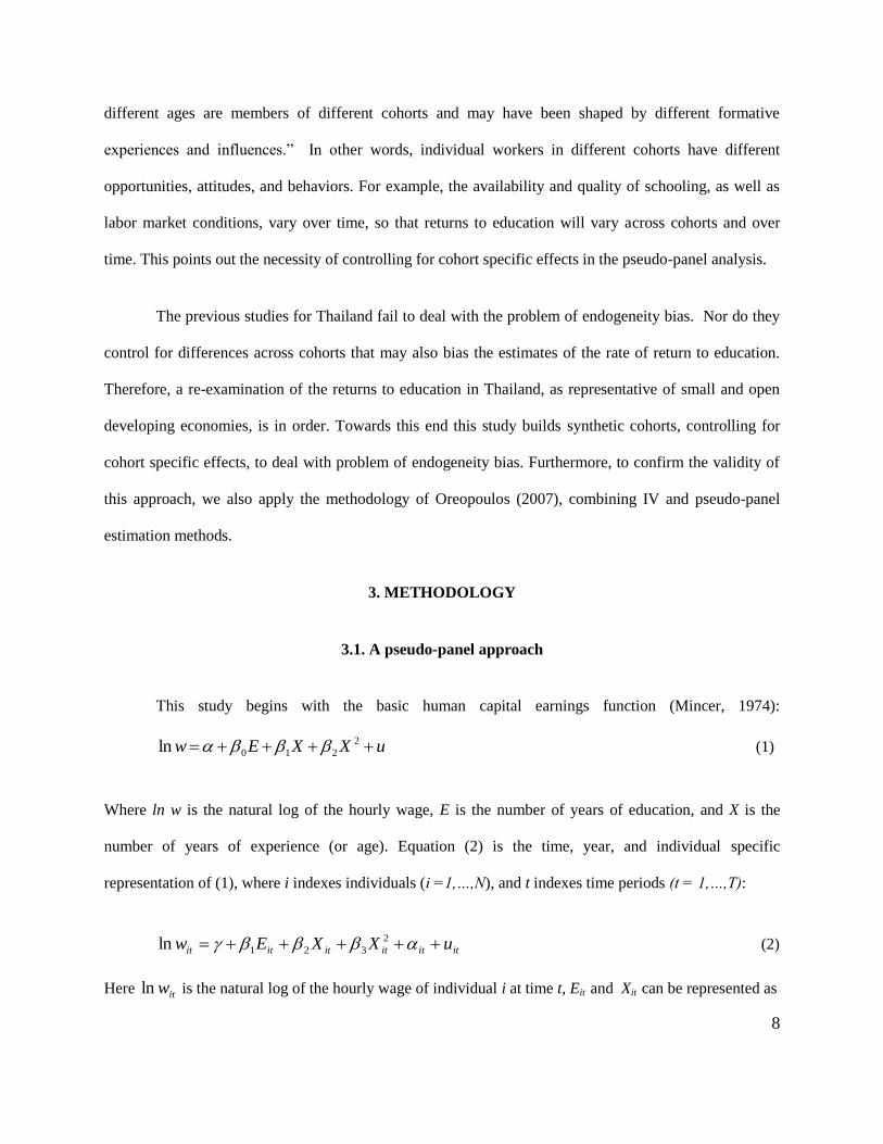
This study begins with the basic human capital earnings function (Mincer, 1974):

uXXEw 2

210ln (1)

Where ln w is the natural log of the hourly wage, E is the number of years of education, and X is the

number of years of experience (or age). Equation (2) is the time, year, and individual specific

representation of (1), where i indexes individuals (i =1,…,N), and t indexes time periods (t = 1,…,T):

itititititit uXXEw 2

321ln (2)

Here itwln is the natural log of the hourly wage of individual i at time t, Eit and Xit can be represented as

9

years of education and years of experience (or age) of individual i at time t, respectively. Then, it

captures unobserved individual heterogeneity, which could be different abilities or motivation levels

across individuals. Even though this model assumes itu is uncorrelated with Eit , Xit , and it , it may be

correlated with Eit. It is not possible to include the “ability” variable into the equation or directly use

individual fixed effects for controlling unobserved individual heterogeneity when estimating (2) with

individual survey data, so that least squares estimates of (2) will be biased and inconsistent.

To solve this problem, Deaton (1985) defines a set of C (c=1,…,C) cohorts, based on year-of-

birth. By tracking birth year cohorts, we then average over the cohort members to obtain an equation

expressed in terms of cohort means, which become the units of observation in the pseudo-panel

estimation. Averaging (2) over the cohort members eliminates the individual heterogeneity such as the

differing abilities or motivations across individuals.

ctctctctctct uXXEw 2

321ln (3)

In equation (3), ctwln is the mean of wln over sample observations in cohort c at time t. Deaton

(1985, p.116) defines ct as the “average of the fixed effects” for those individuals in cohort c in the year

of survey t; ct is not “constant over time” because the samples are collected individually at different

times. As a result, ct may be correlated with ctE , or 0),cov( ctcct E in small samples where

c is the “true cohort effect” (Devereux, 2007).

However, ct can be treated as the true cohort effect ( c ) or the unobserved cohort fixed effect,

if the sample size in each cohort is sufficiently large. Verbeek and Nijman (1992, 1993) find that cell

sizes greater than 100 observations per cell are sufficient to nearly eliminate the bias. In this case

10

cct and we can estimate equation (3) by using cohort dummies (or c ) or cohort fixed effects2 as in

equation (4).

ctcctctctct uXXEw 2

321ln (4)

Estimation of (4) is based on cohort means for each year. In (4) all error components in (2) that are

correlated with explanatory variables have been purged from the error term, so that fixed effects

estimation of this equation expressed in terms of cohort means is consistent. Not only does estimation of

(4) deal with problems of individual heterogeneity while controlling for cohort effects, the use of cohort

means can “average out” individual measurement errors (Antman and McKenzie, 2007).

Since the number of observations per cell varies substantially, the disturbance term ( ctu ) is

heteroskedastic, leading to biased standard errors. We correct this heteroskedasticity using weighted least

squares (WLS) estimation by weighting each cell with the square root of the number of observations in

each cell (Dargay, 2007). In this study estimates are presented based on a pseudo-panel data set with one-

year cohorts and another with two-year cohorts to check the sensitivity of estimates to cell sizes.

3.2. Instrumental variable estimation

In order to confirm the validity of the pseudo-panel approach for the estimation of equation (4),

we also employ IV estimation to individual data set (equation (2)) and also to the pseudo-panel data set

(without including cohort fixed effects (equation (3)). If the pseudo-panel approach (with cohort fixed

effects) is successful in eliminating the endogeneity bias problem, then the pseudo panel and IV estimates

will be similar. Comparison of the two sets of estimation results, in particular their standard errors, also

demonstrates the advantage of the pseudo panel method for this data set.

11

The challenge in IV estimation is finding an instrument that is exogenous with respect to the

earnings equation and yet has significant effects on the endogenous schooling variable. Following Card

(1995) and Uusitalo (1999) a dummy variable identifying the provinces in which universities or teacher

training colleges are located is chosen as an instrument. The exogeneity assumption for this instrument is

tenable if these institutions were put into place prior to the beginning of the sample period (see discussion

in the data section). The presence of a university or teaching training facility in a province is expected to

lower the costs of education and shift preferences towards increased levels of education, and therefore

have an effect on the number of years of schooling. Whether this effect is significant so that this variable

is not a weak instrument is an empirical matter that is revealed by the first stage estimates.

The first stage of the IV regression with the individual data set is:

ititititit uXXE 2

210 (5)

where it is in the dummy variable identifying the provinces that have a university and/or a teacher

training college. Moreover, estimation with pseudo-panel data but without cohort fixed effects will also

be biased if the error term in (3) is correlated with mean levels of schooling. Therefore IV estimation is

appropriate for equation (3) as well, and should produce estimates comparable to the pseudo-panel

estimates of (4).

The first stage of the IV regression for the pseudo-panel data set is:

ctctctctct uXXE 2

210 (6)

where ct is the cohort mean of it . The alternative pseudo-panel estimates (with and without cohort

fixed effects) and the different IV estimates (with individual data and also applied to cohort means) are

12

compared with estimates from a least squares regression on individual data to see the effects of these

alternative methods for controlling individual heterogeneity.

In addition, to control for possible biases arising from aggregation of the data, the estimates from

the full sample are supplemented with results from samples disaggregated by demographic characteristics

including gender, rural/urban residence, and marital status. Disaggregation by demographic groups also

allows estimates of the returns to education to differ across categories, with possible policy implications

following from these differences.

Since other individual and household characteristics from the survey are preserved in the cohort

means, additional background characteristics could be included as controls in the wage equation.3

However, as emphasized by Psacharopolos and Patrinos (2004), inclusion of additional controls can result

in underestimates of the returns to education. Furthermore, Grilliches (1977) points out that additional

controls can increase the impact of measurement error in the schooling variable, thereby increasing the

bias in the returns to education estimates. For comparability with other studies that apply the basic

Mincerian equation, further controls are not included beyond those already described.

4. DATA AND VARIABLES

Construction of a pseudo-panel (Deaton, 1998) starts by using the age of each individual at the

time of the survey to establish the birth cohort to which they belong. The construction assumes that if a

worker is X years of age in year t, then in year t+1, this worker has an age of X+1 years. For example, age

19 in 1986 will be age 20 in 1987, and then will be age 21 in 1988 and so on. This assumption allows the

construction of a panel from the cross-sectional surveys, in which the birth-year cohorts are the cross

sectional dimension of the panel. Data on each birth-year cohort are observed over time.

13

For every survey year the individual observations on the variables of interest are averaged over

each birth cohort, creating cohort-year averages as the units of observation. Cohorts are defined for birth

years from 1946 to 1967 using data from surveys for 1986 through 2005. This establishes age 19 (e.g., in

1986 from the first birth cohort) as the youngest individuals in the sample.

There are 199,833 individual observations from which to build the pseudo-panels. The first data

set pools data from 22 single year-of-birth cohorts and 20 survey years for a total of 440 cohort-year

observations. In every case cell sizes exceed 100, and the vast majority contains over 200 individuals.

The second data set consists of two-year cohorts. Only two cells contain fewer than 300 individuals in

this case, and the total number of observations available for estimation is 220 cohort-year groups (11

cohorts times 20 survey years). Additional pseudo-panels are defined from disaggregations according to

gender, place of residence, and marital status using the two-year cohort design in order to maintain

adequate cell sizes.

The data were collected by the National Statistical Office of Thailand (NSO), Statistical

Forecasting Bureau, as part of the National Labor Force Surveys (LFS) for 1986-2005. Each quarterly LFS

represents data compiled from interviews with the head of household or members of household, with

70,000-200,000 people representing 0.1-0.5% of the total Thai population. For the years 1985-1999, data

are available for only the first and third quarters, but from 2000, the NSO began collecting data every

quarter.

This study employs third quarter data in the estimation in order to control for the effect of

seasonal agricultural labor movements. The concern is that the data from other quarters of the survey may

record as urban workers some rural residents who have temporarily migrated to and are working in the

cities. Thai agricultural workers migrate to work in the cities during the dry season, but return home

during the rainy season of the third quarter (Sussangkarn and Chalamwong, 1996), and they should

therefore be recorded as rural residents and workers during the third quarter survey. This choice of survey

14

quarter is designed to minimize errors in the classification of workers’ residence due to seasonal back and

forth movements between rural and urban areas. The sample is limited to people whose working hours are

equal to or greater than 30 hours a week, and those of ages 19-59 at the time of each survey. This sample

design eliminates individuals who might be working part-time while still in school or partially retired.

The three primary variables of this study are hourly wages, years of education, and age. The

hourly wage is constructed from the monthly wage recorded in the survey using the reported number of

hours of work.4 This nominal wage is deflated by the Thailand Consumer Price Index (CPI)

5. The LFS

records the highest attained degree, and these data are converted into years of education ranging from

zero (no education) to 23 years for those with PhDs. Age is reported directly in the LFS, and this variable

is entered into the regressions in both linear and squared terms.

Finally, for the IV estimation, we identify the provinces in Thailand that have a university and/or

teacher training college (now called “Rajchabat Universities”). Of Thailand’s 76 provinces 35 have a

university and/or a Rajchabat University (Office of the Higher Education Commission, 2010). Provinces

with universities are limited to those with one of the first eight public universities, all established between

1910s and 1970s, and located in Bangkok and in three other major provinces (World Bank, 2010). Forty-

one Rajchabat Universities, located in 35 provinces, were established primarily between the 1920s and the

1970s (Office of the Higher Education Commission, 2010).

5. RESULTS AND DISCUSSION

5.1. Aggregated estimates

The estimates from the regressions with individual data, one-year cohort means, and two-year

cohort means are presented in table 1. Column (i) shows the results from a cross-sectional regression with

15

OLS on individual data, and column (ii) shows the results from the same data using IV. The estimates

from the pseudo-panel method are presented in columns (iii)-(viii).

[Table 1 approximately here]

Columns (iii)-(v) show the results from one year cohort means, to compare with the estimates

based on two-year cohorts (columns (vi)-(viii)). Although the cell sizes in the latter case exceed 283 vs.

only 112 for the single year cohorts, the similarities between these two sets of estimates indicate no

apparent biases with the smaller cell sizes. This evidence is consistent with Verbeek and Nijman (1992,

1993), who contend that 100 observations per cell is sufficient to minimize biases in a pseudo-panel

estimation.

Furthermore, comparisons between columns (iii) and (v) and across (vi) and (viii) show that

controlling for cohorts has an important impact on the estimates with a pseudo-panel data set6. Failure to

control for cohort specific effects in the pseudo-panel approach results in a correlation between the

schooling variable and the error term, thus biasing estimation of the returns to education. This is

demonstrated by the similarity between the OLS estimates from individual data (column i) and those

based on the pseudo-panel data, absent controls for cohort specific effects (columns iii and vi). This

verifies Deaton’s (1985) point that cohort fixed effects must be included in the pseudo-panel regressions

in order to extract the dependence between the regressor and the error term that exists in equation (3).

The basic finding of Table 1 is that the estimated returns to education from the pseudo-panels

with cohort fixed effects (column (v) and (viii)) are considerably larger than those from regressions with

individual data (column (i)) and from the pseudo-panels without cohort fixed effects (column (iii), and

(vi)). This implies that the failure to control for unobservable individual or cohort-specific characteristics

results in a downward bias of the estimated returns to education. In fact, the magnitude of this bias is

substantial, with returns to education underestimated by as much as 28 percent from a comparison of

columns (i) and (viii). Furthermore, the use of instrumental variables estimation on the individual data set

and with the pseudo-panel without cohort fixed effects, (columns (ii), (iv), and (vii)) produces estimates

16

that are in the same range as those from the correctly specified pseudo-panel regressions (column (v) and

(viii)). Apparently, the pseudo-panel and IV approaches are both successful in correcting the biases

arising from unobservable heterogeneity in the individual data OLS regressions.

In the pseudo-panel fixed effects regressions and from the IV estimations, the coefficient on years

of education ranges between 0.141 and 0.160, compared with 0.115 from the individual regression This

last estimate is in the 8% - 12% range of estimates presented in previous cross-sectional studies of Thai

workers cited in section 2, and also comparable to the Asian average of 9.6% reported by Psacharopolos

(1994). The evidence from table 1 indicates that the rate of return to education in Thailand is considerable

higher than previously estimated, with important implications for policy as discussed below.

The downward bias in the OLS regressions with individual data is contrary to some expectations

about the nature of “ability bias” in returns to education studies. However, this finding is consistent with

the optimal choice of schooling model presented by Griliches (1977), in which highly motivated

individuals face high opportunity costs of continuing their education in the face of attractive wage earning

options. This schooling optimizing behavior can give rise to a negative association between the schooling

variable and the equation error that contains the unobservable individual motivation factor and thus

account for the downward bias found here. This effect may be strengthened if the direct costs of

schooling are substantial and there is little opportunity to finance education by borrowing or

intergenerational transfers.

With the complete sample the IV and pseudo-panel methods produce similar results, so that both

procedures effectively treat the problem of endogeneity bias. With the data disaggregated by demographic

characteristics, advantages for the pseudo-panel method emerge. The IV standard errors are invariably

larger than those from the pseudo-panel method. Also, when some disaggregations overlap closely with

the constructed instrument, the IV method yields implausible point estimates with very large standard

errors. For these reasons the following sections discuss only the pseudo-panel estimates. Furthermore,

17

Table 1 shows the importance of including cohort fixed effects in order to treat the endogeneity problem,

so subsequent pseudo-panel estimates are based on this specification.

5.2. Disaggregation by gender

In addition to an overall estimate of the returns to education, policy prescriptions may be

informed by differences in these returns broken down by demographic groups. Disaggregation by

demographic characteristics can also cast light on aggregation bias as an alternative explanation for the

bias in the individual data estimates. In particular, the sample is disaggregated across three alternative

demographic dimensions: gender, place of residence, and marital status. Since disaggregation reduces the

numbers of observations in each cell in the pseudo-panels, these disaggregated panels are constructed

using two-year cohorts.

Table 2 shows the regression results of equation (4) with the disaggregated data set, which has

been stratified by men and women. Overall, the results in table 2 confirm the main results in table 1,

showing the downward bias in cross-sectional regressions on individual data. The coefficients on years of

education for men and women from the cross-sectional regression are 0.107 and 0.129, respectively

(columns (i) and (iii)), while, from the pseudo-panel approach with two-year cohort means they are

around 0.126 for men and 0.178 for women. This disaggregation shows the rate of return to education for

women is higher than for men, a result that is consistent with the many studies using US data (Dougherty,

2005)7, but contrasts with some studies for Thailand (see section 2). Dougherty’s explanation of the

higher rate of return for women is that education helps women find employment outside “the low-paying

traditionally female occupations”.

[Table 2 approximately here]

The downward bias in the returns to education estimate from the individual data regressions

remains with disaggregation by gender. In addition, the difference between the individual data estimate

and the pseudo-panel value is greater for women (0.05=0.18-0.13) than for men (0.02=0.13-0.11).

18

Applying the opportunity cost argument presented above, this difference could mean that high ability men

have greater educational access than women, due to the attitudes and conventions of Thai society during

the 1950s-1960s. During this early period of development, there was discrimination against girls in

education (Thosanguan, 1978). Gandhi-Kingdon (2002) defined this as “unexplained parental

discrimination”, with differential support for educating boys over girls. A girl with abilities equal to a

boy’s would receive less family support for schooling, thus strengthening the negative correlation

between years of education and ability for girls compared with boys, and increasing the downward bias

observed for females.

5.3. Rural Vs. Urban disaggregation

Table 3 displays the individual and pseudo-panel estimates separately for urban and rural

residents. Overall, these estimates are consistent with the main results in table 1, again showing the

downward bias in cross-sectional regressions on individual data. From the pseudo-panel estimates the

coefficient on years of schooling is higher for those living in urban areas (0.189) compared with that for

rural residents (0.142). This is consistent with the expectation that individuals living in urban areas have

more opportunities to exploit skills acquired through higher education than do those living in rural areas.

[Table 3 approximately here]

The gap between pseudo-panel and individual data estimates of the returns to education indicate a

larger bias for urban (0.189-0.115=0.074) versus rural workers (0.142-0.113=0.029). Given higher

relative wages in urban areas, the opportunity cost of studying for urban residents is higher than for those

in rural areas, so that the schooling optimization decision leads to an earlier departure from school for

highly motivated individuals. In addition, people living in rural areas may be able to work on their farms

at the same time as studying, so that the opportunity cost of studying for rural areas is lower than for

19

urban areas. These differences in opportunity costs may account for the greater downward bias in the

estimate of the returns to education for urban compared with rural workers.

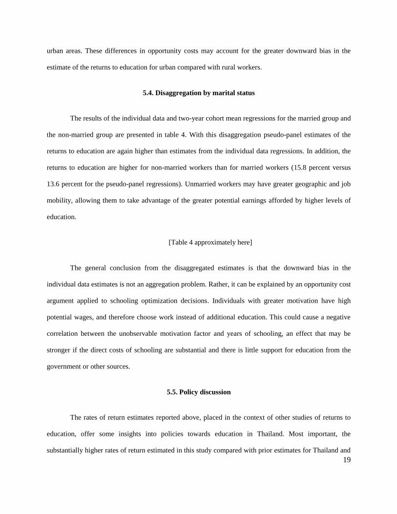
5.4. Disaggregation by marital status

The results of the individual data and two-year cohort mean regressions for the married group and

the non-married group are presented in table 4. With this disaggregation pseudo-panel estimates of the

returns to education are again higher than estimates from the individual data regressions. In addition, the

returns to education are higher for non-married workers than for married workers (15.8 percent versus

13.6 percent for the pseudo-panel regressions). Unmarried workers may have greater geographic and job

mobility, allowing them to take advantage of the greater potential earnings afforded by higher levels of

education.

[Table 4 approximately here]

The general conclusion from the disaggregated estimates is that the downward bias in the

individual data estimates is not an aggregation problem. Rather, it can be explained by an opportunity cost

argument applied to schooling optimization decisions. Individuals with greater motivation have high

potential wages, and therefore choose work instead of additional education. This could cause a negative

correlation between the unobservable motivation factor and years of schooling, an effect that may be

stronger if the direct costs of schooling are substantial and there is little support for education from the

government or other sources.

5.5. Policy discussion

The rates of return estimates reported above, placed in the context of other studies of returns to

education, offer some insights into policies towards education in Thailand. Most important, the

substantially higher rates of return estimated in this study compared with prior estimates for Thailand and

20

East Asia emphasize the importance of investments in human capital as a component of economic growth

policy. Psacharopolos and Patrinos (2004) reports an average rate of return of ten percent for Asia as a

whole, and a rate of 11.5 percent for Thailand, citing the study by Patrinos (1995), compared with

estimates ranging between 14 and 16 percent from the pseudo-panel estimation. Consequently, increased

private or public investments in education are expected to yield additions to incomes that are 22 to 40

percent higher than was previously estimated for Thailand.

Added to these high estimated private returns, gains to society as a whole are expected to be even

larger due to a variety of spillover effects. First among these are productivity gains experienced by a

cohort of workers as a result of the increased levels of education of others in the same cohort (Lucas,

1988). These economy-wide productivity effects may be reflected in macro level data, for example, in

growth regressions. Studies of the strong record of economic growth in Asian economies point to

education as the single largest explanation of the higher growth rates in Asia compared with other regions

of the world (World Bank, 1995). In addition, investments in education provide positive spillovers in the

form of political stability, social cohesion, and enhanced productivity of physical capital (McMahon,

1998). These spillovers imply a social rate of return that is higher than the private rate, so that even the

large estimated returns reported here provide only lower bounds to the estimates of overall societal gains

from investments in education.

These spillovers also provide an efficiency argument for public support of education.

Governments can expand levels of education in a variety of ways: compulsory schooling, public funding

of school construction and operating expenses, subsidies of teacher training, and financial incentive for

parents who keep their children in school such as the Progressa Program in Mexico and Borsa Familia in

Brazil. To the extent that public subsidies of schooling represent a larger portion of household income for

poor families relative to higher income households, government support of education leads to great

equality in education and hence in incomes. Increased income equality tends to increase social cohesion,

21

providing a further efficiency argument in favor of public support of education (Fuente and Ciccone,

2003).

A consistent finding across studies of returns to education, including the present investigation, is

that females experience a higher rate of return than males (Psacholopolos 1994; Psacholopolos and

Patrinos 2004). Schultz (2002) attributes this to a lower average level of education for women, together

with diminishing returns to higher levels of schooling. In Thailand, however, this is not the case, with the

average number of years of schooling for females exceeding that for males by nearly one and one half

years throughout the years of the survey data employed here (1986 to 2005). In any case, this sex

differential provides a direct efficiency argument in support of increased schooling of girls in terms of the

higher private returns from each extra year of education. In addition, there exist important spillovers from

female education in the form of improved child health, reduced fertility, and an increased tax base due to

the higher labor force participation rates of educated women (Schultz, 2002). Education policy can be

designed to promote schooling for girls, for example, with schools or classrooms segregated by gender,

greater employment of female teachers, locating schools close to residences, and designing school hours

that do not conflict with girls’ household duties (World Bank, 1995).

The estimates in Table 3 show the rate of return for urban workers (19 percent) to be sharply

higher than for rural workers (14 percent). This is the reverse of estimates for Africa, where increased

farm productivity due to education provides an important source of income gains for rural workers

(McMahon, 1987). However, the survey instrument used in the current study asks respondents to report

“wages”, not a more comprehensive income measure that would include farm revenues. In any case,

Thailand’s export-led growth strategy has emphasized investment in manufacturing industries, such that

the strong demand for skilled labor in urban areas has produced higher rates of returns to education. The

urban-rural differential in returns to education, together with lower average years of schooling in rural

areas (a difference of one and one-half years in 2005), has created substantial disparities in average

22

incomes between these geographic areas and encouraged seasonal and permanent migration to the cities.

To reduce these regional disparities the government of Thailand could increase access to schools in rural

areas and promote the development of industries in rural areas through tax incentives and improvements

in infrastructure.

The returns to education estimates from the pseudo-panel method lead to several policy

recommendations. The high rate of return estimated for the entire sample indicates that investments in

education account for some of the high rates of growth and increases in per capita incomes experienced

by Thailand over the past twenty years. Spillovers added to these high private returns provide justification

for public support of education. The higher rate of return estimated for female workers compared with

males justifies increased schooling for girls on efficiency grounds, and this argument is augmented by

additional spillovers in the form of improved child health and education of the next generation. Finally,

the finding that rural returns fall short of those for urban workers leads to suggestions for policies that

could improve earning capacities for rural workers by increased access to schools and promotion of rural

industries.

6. CONCLUSION

This study applies a pseudo-panel approach to estimate the rate of return to education in Thailand

for workers born between 1946 and 1967. This approach controls for unobservable individual

characteristics, such as ability or motivation, that may bias the estimated rate of return to education. One

strong result is that there is a downward bias in the estimates of the rate of return to education based on

individual data. This result holds for several disaggregations of the data by demographic characteristics,

ruling out the aggregation bias explanation. Alternatively, the downward bias is explained by a schooling

optimization argument. Individuals with greater motivation have high potential wages, and therefore

choose to enter the labor force rather than continue their education. This would imply a negative

23

correlation between motivation and years of schooling, and with a positive correlation between

motivation and earnings, the individual data regressions would show a negative endogeneity bias due to

this omitted factor.

Based on the pseudo-panel estimations, the overall rate of return to education in Thailand is

between 14% and 16%, which is considerably higher than estimated in prior studies that have used

individual data from Thailand. Additional findings are that returns to education are higher for females

than for males, and unmarried individuals show higher returns than married workers. Not surprisingly,

urban workers receive higher returns to education than rural workers due to their greater opportunities to

exploit their increased skills in the cities.

The comparatively high rate of return to education found here, together with the differential rates

of return found when the sample is disaggregated, lead to several policy recommendations. The high

overall estimated rate of return indicates that investments in education can account for a portion of the

high rates of growth and increases in per capita incomes experienced by Thailand over the past twenty

years. The higher rate of return estimated for female workers compared with males justifies increased

schooling for girls on efficiency grounds, an argument that is strengthened by the existence of spillovers

in the form of improved child health and education of the next generation.

24

NOTES

1 According to Psacharopoulos and Patrinos (2004), there were ninety-eight countries, including both developed

countries and developing countries, with estimates of rates of return to education. The average rate of return to

education across these studies is 10%. Also, this rate tends to be higher in the developing countries than in

developed countries, and women tend to have a higher rate of return than men.

2 Note that we do not incorporate year dummies (or year fixed effects) into the equation because cohort dummies (or

cohort fixed effects) can capture the differences across cohorts. Thus, inclusion of cohort dummies is similar to what

we can see over time; inclusion of year dummies would be redundant. Furthermore, when we test by including year

dummies in the estimation, the results from inclusion or exclusion of year dummies are similar.

3 Parental background characteristics are sometimes included in returns to education studies, but these variables are

not available in the Thai Labor Force Surveys.

4 Welsh (1997) discusses the problem of constructing hourly wages from annual earnings, weeks, and hours per

week in the estimation of the responsiveness of labor supply to hourly wage rates. A problem of “division bias” can

arise with errors in reporting hours of work when both dependent and independent variables involve this noisy

measure (Borjas, 1980). In this study, however, wages only appear as the dependent variable, avoiding this concern.

The hourly wage is constructed from the monthly wage dividing by 4 to obtain weekly wage and further dividing by

reported weekly hours to obtain the hourly wage.

5 The CPI indexes (2002 as a base year) are from the Bureau of Trade and Economic Indices, Ministry of

Commerce, Thailand

6 To check the robustness of the pseudo-panel design, the first and last cohorts are dropped from the sample, and the

remaining cohorts are recombined into different two-year groupings. This results also in a change in sample size

25

with 400 cohort-year observations constructed from 184,093 individual data points. With this new pseudo-panel the

coefficients on years of education and other coefficient estimates are similar to those from the full sample.

7 Dougherty (2005) draws this conclusion from 28 US studies on the rate of return to education between men and

women.

26

REFERENCES

Amornthum, S., & Chalamwong, Y. (2001). Rate of Return to Education. Human Resources and the

Labor Market of Thailand. Bangkok, Thailand: Thailand Development Research Institute (TDRI).

Angrist, J. D., & Krueger, A. B. (1991). Does compulsory school attendance affect schooling and

earnings?. Quarterly Journal of Economics, 106(4), 979-1014.

Antman, F., & Mckenzie, D. J. (2007). Poverty traps and Nonlinear Income Dynamics with Measurement

Error and Individual Heterogeneity. Journal of Development Studies, 56, 125-161.

Appiah, E. N., & McMahon, W. W. (2002). The social outcomes of education and feedbacks on growth in

Africa. Journal of Development Studies, 38, 27–68.

Ashenfelter, O., Harmon, C., & Hessel, O. (1999). A Review of Estimates of the Schooling/Earnings

Relationship, with tests for Publication Bias. Labor Economics, 6(4), 453-470.

Borjas, G. (1980). The relationship between wages and weekly hours of work: the role of division bias.

Journal of Human Resources, 15(3), 409-423.

Bureau of Trade and Economic Indices, Ministry of Commerce, Thailand [http://www.price.moc.go.th].

Bound, J., Jaeger, D., & Baker, R. (1995). Problems with Instrumental Variables Estimation When the

Correlation between the Instruments and the Endogenous Explanatory Variable Is Weak. Journal of the

American Statistical Association, 90(430), 443-50.

Blundell, R., Dearden, L., & Sianesi, B. (2001). Estimating the Returns to Education: Models, Methods

and Results. London: Centre for the Economics of Education, London School of Economics.

Card, D. (1995). Using Geographic Variation in College Proximity to Estimate the Return to Schooling.

In L.Christofides, K.Grant, & R. Swindinsky (Eds.), Aspects of Labour Market Behaviour: Essays in

Honour of John Vanderkamp, Toronto: University of Toronto Press.

Card, D. (1999). The Causal Effect of Education on Earnings. In O. Ashenfelter, & D. Card (Eds.),

Handbook of Labor Economics, 3A, Amsterdam and New York: North Holland.

27

Card, D. (2001). Estimating the Return to Schooling: Progress on Some Persistent Econometric Problems.

Econometrica, 69(5), 1127-1160.

Card, D. & Lemieux, T. (2001). Can Falling Supply Explain the Rising Return to College for Younger

Men? A Cohort-Based Analysis. The Quarterly Journal of Economics, 116(2), 705-746.

Chiswick, C. (1976). On estimating earning functions for LDCs. Journal of Development Economics, 3,

67-78

Conneely, K. & Uusitalo, R. (1997). Estimating heterogeneous treatment effects in the Becker schooling

model. Mimeo, Industrial Relation Section, Princeton University.

Dargay, J. 2007. The effect of prices and income on car travel in the UK. Transportation Research Part

A, 41, 949-960.

Deaton, A. (1985). Panel data from a time series of cross-sections. Journal of Econometrics, 30, 109-126.

Deaton, A. (1998). The Analysis of Household Surveys: A Microeconometric Approach to Development

Policy. Baltimore, MD: The Johns Hopkin Univesity Press.

Devereux, P. (2007). Small-sample bias in synthetic cohort models of labor supply. Journal of applied

econometrics, 22, 839-848.

Dougherty, C. (2005). Why Are the Returns to Schooling Higher for Women than for Men?. Journal of

Human Resources, 40(4), 969-988.

Fuente, A. & Ciccone, A. (2003). Human capital in a global and knowledge-based economy. UFAE and

IAE Working Papers 562.03. Unitat de Fonaments de l'Anàlisi Econòmica (UAB) and Institut d'Anàlisi

Econòmica (CSIC).

Gandhi-Kingdon, G. (2002). The gender gap in educational attainment in India: how much can be

explained?. The Journal of Development Studies, 39(2), 25-53.

Glenn, N. (2005). Cohort Analysis. Thousand Oaks, CA: Sage Publications.

Grilliches, Z. (1977). Estimating the Returns to Schooling: Some Econometric Problems. Econometrica,

45(1), 1-22

28

Harmon, C. & Walker, I. (1995). Estimates of the Economic Return to Schooling for the United

Kingdom. American Economic Review, 85(5), 1278-86.

Hawley, J. (2004). Changing returns to education in times of prosperity and crisis, Thailand 1985-

1998. Economics of Education Review,23, 273-286.

Heckman, J., Lochner, L., & Petra, T. (2005). Earnings functions, Rate of return, and Treatment Effects:

The Mincer Equation and Beyond. NBER Working Paper: 11544.

Kane, T. & Rouse, C. (1993). Labor Market Returns to Two-and Four-Year Colleges: Is a Credit and Do

Degree Matter?. NBER Working Papers: 4268.

Lucas, R. E. (1988). On the mechanics of economic development. Journal of Monetary Economics, 22,

3–22.

McMahon, W. W. (1987). The Relation of Education and R&D to Productivity Growth in the Developing

Countries of Africa. Economics of Education Review, (6) 2, 183-194.

McMahon, W. W. (1998). Education and growth in East Asia. Economics of Education Review, 17(2),

159–172.

McMahon, W.W. (1999). Education and development: Measuring the social benefits. New York: Oxford

University Press.

McMahon, W. W. (2001). The Impact of Human Capital on Non-Market Outcomes and Feedbacks on

Economic Development. In J. Helliwell (Ed), The Contribution of Human and Social Capital to Sustained

Economic Growth and Well-Being(pp.136-71), Paris: OECD.

Mincer, J. (1974). Schooling, Experience, and Earnings. New York: National Bureau of Economic

Research.

OECD (2000). Estimating Economic and Social Returns to Learning: Session 3 Issues for Discussion.

OECD.

Office of the Higher Education Commission, Ministry of Education, Thailand 2010

[http://www.mua.go.th]

29

Oreopoulos, P. (2007). Do dropouts drop out too soon? Wealth, health and happiness from compulsory

schooling. Journal of Public Economics, 91(11-12), 2213-2229.

Patrinos, H. A. (1995). Education and earnings differentials. Mimeo, Washington, DC: World Bank.

Psacharopoulos, G. (1994). Returns to investment in education: a global update. World Development.

22(9), 1325–1343.

Psacharopoulos, G. & Patrinos, H.A. (2004). Returns to investment in education: A further update”.

Education Economics, 12(2), 111-134.

Schultz, P. (2002). Why Governments Should Invest More to Educated Girls. World Development, 30 (2),

207-225.

Sussangkarn, C. & Chalamwong, Y. (1996). Thailand development strategies and their impacts on labour

markets and migration. In D. O’Connor, & L. Farsakh (Eds.), Development strategy, employment, and

migration. Paris: OECD.

Thosanguan, V. (1978). The position of women and their contribution to the food processing industry in

Thailand. Workshop on TCDC and Women at Asian and Pacific Centre for women and development,

Tehran, Iran (24-26 April, 1978).

Uusitalo, R. (1999). Essays in Economics of Education. Unpublished doctoral dissertation, University of

Helsinki, Finland.

Verbeek, M. & Nijman, T. (1992). Can cohort data be treated as genuine panel data?. Empirical

Economics, 17, 9-23.

Verbeek, M. & Nijman, T. (1993). Minimum MSE estimation of a regression model with fixed effects

from a series of cross-sections. Journal of Econometrics, 59, 125-136.

Welsh, F. (1997). Wage and Participation. Journal of Labour Economics, 15(1), 77-103.

World Bank (1995). Priorities and Strategies for Education: A World Bank Review. Washington, DC:

The World Bank.

World Bank (2002). Education and HIV/AIDS: A Window of Hope. Washington, D.C: The World Bank.

30

World Bank (2006). Thailand Investment Climate, Firm Competitiveness and Growth. Washington, D.C.:

The World Bank.

World Bank (2010). Thailand-Towards a Competitive Higher Education System in a Global Economy,

Bangkok, Thailand: The World Bank Group.

31

Table 1: Returns to education estimates for individual data, one-year cohort means, and two-year cohort meansa

Individual

Data

(Cross-

sectional

regression)

OLS

(i)

Individual

Data

(Cross-

sectional

regression)

IV

(ii)

Pseudo-Panel

(One-year

cohort

means)

WLS

(iii)

Pseudo-Panel

(One-year

cohort

means)

WLS-IV

(iv)

Pseudo-Panel

(One-year

cohort

means)

WLS

(v)

Pseudo-Panel

(Two –year

cohort

means)

WLS

(vi)

Pseudo-Panel

(Two –year

cohort

means)

WLS-IV

(vii)

Pseudo-Panel

(Two- year

cohort

means)

WLS

(viii)

Constant

Years of education

Age

Age squared

-0.199

(0.0251)

0.115

(0.000250)

0.0958

(0.00131)

-0.000683

(0.0000169)

-0.216

(0.0639)

0.141

(0.0103)

0.0855

(0.00360)

-0.000553

(0.0000473)

-0.124

(0.0937)

0.101

(0.00729)

0.100

(0.00503)

-0.000740

(0.0000646)

-0.384

(0.140)

0.148

(0.0194)

0.0852

(0.00778)

-0.000544

(0.000101)

-0.471

(0.111)

0.151

(0.0100)

0.0909

(0.00499)

-0.000684

(0.0000629)

-0.108

(0.131)

0.099

(0.0107)

0.101

(0.00702)

-0.000752

(0.0000907)

-0.371

(0.191)

0.146

(0.0262)

0.0860

(0.0105)

-0.000554

(0.000138)

-0.528

(0.162)

0.160

(0.0157)

0.0890

(0.00704)

-0.000665

(0.0000881)

Cohort dummies

Individual observations

Cohort-year observations

Individual observations per

cohort

- Max

- Min

-

199,833

-

-

-

-

199,833

-

-

-

No

199,833

440

1,017

113

No

199,833

440

1,017

113

Yes

199,833

440

1,017

113

No

199,833

220

1,690

284

No

199,833

220

1,690

284

Yes

199,833

220

1,690

284

Adjusted R2

0.591

0.561

0.940

0.934

0.947

0.942

0.938

0.949

a Numbers in parentheses are standard errors. All coefficients are significant at or below the 0.05 level.

32

Table 2: Returns to education estimates for men and womena

Men

Individual Data

(Cross- sectional

regression)

(i)

Men

Pseudo-Panel

(Two-year cohort

means)

(ii)

Women

Individual Data

(Cross- sectional

regression)

(iii)

Women

Pseudo-Panel

(Two -year

cohort means)

(iv)

Constant

Years of education

Age

Age squared

0.128

(0.0350)

0.107

(0.000342)

0.0880

(0.00181)

-0.000606

(0.0000231)

-0.0536

(0.161)

0.126

(0.0158)

0.0893

(0.00684)

-0.000679

(0.0000861)

-0.502

(0.0353)

0.129

(0.000362)

0.0985

(0.00187)

-0.000712

(0.0000244)

-0.742

(0.150)

0.178

(0.0130)

0.0825

(0.00718)

-0.000561

(0.0000901)

Cohort dummies

Individual observations

Cohort-year observations

-

112,419

-

Yes

112,419

220

-

87,414

-

Yes

87,414

220

Adjusted R2 0.540 0.944 0.663 0.953

a Numbers in parentheses are standard errors. All coefficients are significant at or below the 0.05 level.

33

Table 3: Returns to education estimates for urban and rural residentsa

Urban

Individual Data

(Cross- sectional

regression)

(i)

Urban

Pseudo-Panel

(Two-year

cohort means)

(ii)

Rural

Individual Data

(Cross- sectional

regression)

(iii)

Rural

Pseudo-Panel

(Two-year

cohort means)

(iv)

Constant

Years of education

Age

Age squared

-0.194

(0.0293)

0.115

(0.000308)

0.0943

(0.00153)

-0.000648

(0.0000197)

-0.713

(0.141)

0.189

(0.0136)

0.0805

(0.00701)

-0.000573

(0.0000868)

-0.298

(0.0491)

0.113

(0.000433)

0.104

(0.00259)

-0.000847

(0.0000335)

-0.424

(0.151)

0.142

(0.0126)

0.0957

(0.00771)

-0.000759

(0.000102)

Cohort dummies

Individual observations

Cohort-year observations

-

135,248

-

Yes

135,248

220

-

64,585

-

Yes

64,585

220

Adjusted R2 0.598 0.958 0.565 0.916

a Numbers in parentheses are standard errors. All coefficients are significant at or below the 0.05 level.

34

Table 4: Returns to education estimates for married and unmarried workersa

Unmarried

Individual Data

(Cross- sectional

regression)

(i)

Unmarried

Pseudo-Panel

(Two-year cohort

means)

(ii)

Married

Individual Data

(Cross- sectional

regression)

(iii)

Married

Pseudo-Panel

(Two-year cohort

means)

(iv)

Constant

Years of education

Age

Age squared

-0.358

(0.0413)

0.126

(0.000508)

0.0959

(0.00231)

-0.000738

(0.0000313)

-0.377

(0.158)

0.158

(0.0110)

0.0788

(0.00736)

-0.000540

(0.0000954)

0.298

(0.0353)

0.112

(0.000284)

0.0746

(0.00179)

-0.000430

(0.0000223)

0.158

(0.118)

0.136

(0.0151)

0.0700

(0.00853)

-0.000438

(0.000101)

Cohort dummies

Individual observations

Cohort-year observations

-

50,977

-

Yes

50,977

220

-

148,856

-

Yes

148,856

220

Adjusted R2 0.619 0.915 0.575 0.957

a Numbers in parentheses are standard errors. All coefficients are significant at or below the 0.05 level.