The Returns to Seniority in France

(and Why they are Lower than in the United States)

Magali Beffy∗ Moshe Buchinsky† Denis Fougère‡

Thierry Kamionka§ Francis Kramarz¶

September 2004

Abstract

In this article, we estimate a joint model of participation, mobility, and wages for France. Our statistical

model allows us to distinguish between unobserved person heterogeneity and state-dependence. The model

is estimated using bayesian techniques using a long panel (1976-1995) for France. Our results show that

returns to seniority are small, even close to zero for some education groups, in France. Because we use the

exact same specification as Buchinsky, Fougère, Kramarz and Tchernis (2002), we compare their results

with ours and show that returns to seniority are (much) larger in the United States than in France. This

result also holds when using Altonji and Williams (1992) techniques for both countries. Most differences

between the two countries relate to firm-to-firm mobility. Using a model of Burdett and Coles (2003), we

explain the rationale for this. More precisely, in a low-mobility country such as France, there is little gain

in compensating workers for long tenures because they will eventually stay in the firm; even when they hold

firm-specific capital. But, in a high-mobility country such as the United States, high returns to seniority have

a clear incentive effect.

Keywords : Participation, Wage, Job mobility, Returns to seniority, Returns to experience, Individual effects.

JEL Classification : J24, J31, J63.

∗ CREST-INSEE (magali.poncon-beffy@ensae.fr)† UCLA, CREST and NBER (buchinsky@econ.ucla.edu)‡ CNRS and CREST (fougere@ensae.fr)§ CNRS and CREST (kamionka@ensae.fr)¶ CREST-INSEE, CEPR and IZA(kramarz@ensae.fr): Corresponding author. We thank Pierre Cahuc, Jean Marc Robin and seminar

participants at Crest, Royal Holloway (DWP conference), Paris-I for very helpful comments. Remaining errors are ours.

1

1 Introduction

In the last twenty years, huge progress was made in the analysis of the wage structure. However, the under-

standing of wage growth - a key issue in labor economics - is not as developed. In particular, the respective

roles of general experience and tenure are still debated. Indeed, experience and tenure increase simultaneously

except when worker moves from firm to firm or becomes not employed. The question of worker mobility and

participation should then be central in the study of wages since it potentially allows the analyst to distinguish

and identify these two components of human capital accumulation. And, therefore, it should help us in assess-

ing the respective roles of general - transferable - human capital and specific - non transferable - human capital.

Of course, the question of the relative importance of job tenure and experience on wage growth has been exten-

sively studied. For the USA, some authors have concluded that experience matters more than seniority in wage

growth (Altonji and Shakotko, 1987, Altonji and Williams, 1992 and 1997). Other authors have concluded

that both experience and tenure matter (Topel, 1991, Buchinsky, Fougère, Kramarz and Tchernis, 2002 BFKT,

hereafter). Indeed, this question is particularly complex to analyze. And, it should not be surprising that the

successive articles have uncovered various crucial difficulties and solutions that potentially affect the resulting

estimates: the definition of the variables, the errors in measured seniority, the estimation methods that are used,

the heterogeneity components of the model, the exogeneity assumptions that are made...

It is usually admitted that there exists an increasing relation between wage and seniority. Several economic

theories can explain the relation existing between wage growth and job tenure. 1) The role of specific job tenure

on the dynamics of wages has been described by human capital theory (Becker (1964), Mincer (1974)). The

central point of this theory is the increase of the earnings due to the individual’s investment in human capital.

2) The structure of wages can be described by job matching theory (Jovanovic, 1979, Miller 1984, Jovanovic,

1984). This theory explains both the mobility of workers from job to job and the existence of an decreasing

job separation rate with job-tenure. This model relies on the main assumption that there exists a productivity

of the worker-occupation pair. This productivity is, a priori, unknown. Of course, the worker’s wage depends

on this productivity. Indeed, the specific human capital investment will be larger when the match is less likely

to terminate (see Jovanovic, 1979). Finally, a job matching model can predict an increase of the worker’s wage

with job seniority. 3) The dynamics of wages can be explained by deferred compensation theories that state

that the form of the contract existing between the firm and employees is chosen such that the worker’s choice

of effort or worker’s quit decision is optimal (see Salop and Salop, 1976; or Lazear 1979, 1981, 1999). In these

theories, the workers starting in a firm are paid below their marginal product whereas the workers with a large

tenure are paid above their marginal product. 4) More recently, equilibrium wage tenure contracts have been

2

shown to exist within a matching model (see Burdett and Coles, 2003 or Postel-Vinay and Robin, 2002 in a

slightly different context). At the equilibrium, firms post a contract that makes wage increase with tenure. Some

of these models are able to characterize both workers mobility and the nature of the relation existing between

wage and tenure. For instance in the Burdett and Coles model, the specificities of the wage-tenure contract

heavily depend on workers’ preferences as well as labor market characteristics job offers arrival rate.

Therefore, the relation between wage growth and mobility (or job tenure) may result from (optimal) choices

of the firm and (or) the worker. But, it may also result from spurious duration dependence. Indeed, if there is

a correlation between job seniority and a latent variable measuring worker’s productivity and if, in addition,

more productive workers have higher wages then there will exist a positive correlation between wage and job

seniority even when conditional wages do not depend on job tenure (see, for instance Abraham and Farber, 1987,

Lillard and Willis, 1978, Flinn 1986). Consequently, unobserved heterogeneity components must be taken into

account as well as the endogeneity of mobility decisions. Furthermore, BFKT showed that mobility-induced

costs translated into state-dependence in the mobility decision (similarly for the participation decision itself

as demonstrated by Hyslop, 1999). As is well-known, all of the above points make OLS estimates of returns

to seniority biased. There are multiple ways to solve this problem. One solution is the use of an instrumental

variables estimator (Altonji and Shakotko, 1987). Another way to go, is to use fixed effects procedures (Abowd,

Kramarz and Margolis, 1999). A final solution is to jointly model wages, mobility and participation decisions

(Buchinsky, Fougère, Kramarz and Tchernis, 2002).

In this paper, we adopt the latter route. Therefore, we estimate jointly wage outcomes, participation and

mobility decisions. The initial conditions are modelled following Heckman (1981). We include both state-

dependence and (correlated) unobserved individual heterogeneity in the mobility and participation decisions.

We also include correlated unobserved individual heterogeneity in the wage equation. Following BFKT, we

adopt a Bayesian framework in which the model is estimated using a Gibbs Sampling technique. As our model

is highly non-linear, we use data augmentation steps. This procedure allows us to obtain, at the stationarity of

the algorithm, estimates of the parameters.

Our data source results from the match of the French DADS panel (giving us wages for the years 1976

to 1995) with the Echantillon Démographique Permanent (EDP, hereafter) that yields time-varying and time-

invariant personal characteristics. Because we use the exact same specification as BFKT and relatively similar

data sources, we are able to compare French returns to seniority with those obtained for the United States. Even

though our estimates of the returns to seniority appear to be in line with those obtained by Altonji and Shakotko

(1987) and Altonji and Williams (1992, 1997) for the U.S., they are in fact much smaller than those obtained

by BFKT (also for the U.S.). Indeed, returns to seniority in France are virtually equal to zero. However, returns

3

to experience are rather large and close to those estimated by BFKT.

To understand some of the reasons for these small returns in comparison to the United States, we make use

of the equilibrium search model with wage-contracts proposed by Burdett and Coles (2003). We show that,

for all values of the relative risk aversion coefficient, the larger the job arrival rate, the steeper the wage-tenure

profiles. And, indeed, recent estimates show that the job arrival rate for the unemployed is approximately equal

1.71 per year in the US and is approximately equal to 0.56 per year in France (Jolivet, Postel-Vinay and Robin,

2004). Hence, the returns to seniority directly reflect the patterns of mobility in the two countries.

This paper is organized as follow. Section 2 presents the statistical model. Section 3 explains elements of

the estimation method. Then, data sources are presented in Section 4. Section 5 shows our estimates whereas

Section 6 carefully compares our results with those obtained by BFKT for the US. This Section also contains a

theoretical explanation of these differences together with simulations. Finally, Section 7 concludes.

2 The Statistical Model

2.1 Specification of the General Model

We consider a joint model of wages, participation and mobility decisions. Following Heckman (1981), we

introduce initial conditions because of the presence of lagged mobility and participation decisions in the main

participation and mobility equations. The statistical model that we adopt here derives directly from a structural

choice model of participation and mobility (see BFKT for a proof). This model induces the following equations:

Initial Conditions

yi1 = I(XY

i1δY0 + αY,I

i + vi1 > 0)

(1)

wi1 = yi1

(XW

i1 δW + θW,Ii + εi1

)(2)

mi1 = yi1I(XM

i1 δM0 + αM,I

i + ui1 > 0)

(3)

4

Main Equations

∀t > 1, yit = I

γMmit−1 + γY yit−1 + XY

it δY + θY,Ii + vit︸ ︷︷ ︸

y∗it

> 0

(4)

∀t > 1, wit = yit

(XW

it δW + θW,Ii + εit

)(5)

∀t > 1, mit = yit.I

γmit−1 + XM

it δM + θM,Ii + uit︸ ︷︷ ︸

m∗it

> 0

(6)

yit andmit denote, respectively, participation and mobility, as previously defined.yit is an indicator func-

tion, equal to1 if the individual i is employed at datet. mit is an indicator function that takes the following

values:

yit+1 = 1 yit+1 = 0yit = 1 mit = 1 if J(i, t + 1) 6= J(i, t) mit censored

mit = 0 if J(i, t + 1) = J(i, t)yit = 0 mit = 0 p.s. mit = 0 p.s.

Table 1: Mobility

whereJ(i, t) denotes the firm at which individuali is employed at datet.

The variablewit denotes the logarithm of the annualized total labor costs. The variablesX are the observ-

able time-varying as well as the time-invariant characteristics for individuals at the different dates.

θI denote the random effects specific to the individuals.u, v andε are the error terms. There areJ firms

andN individuals in the panel of lengthT . Notice that our panel is unbalanced. All stochastic assumptions are

described now.

2.2 Stochastic Assumptions

The next equations present our stochastic assumptions for the individual effects:

θI =(αY,I , αM,I , θY,I , θW,I , θM,I

)of dimension [5N, 1]

5

Moreover, let us assume that1

θIi |ΣI

i ∼ N (0,ΣIi )(7)

where the variance-covariance matrix in this prior distribution has the following form:

ΣIi = Di∆ρDi with(8)

∆ρ = CC ′ where(9)

C =

1 0 0 0 0

cos1 sin1 0 0 0

cos2 sin2 cos3 sin2 sin3 0 0

cos4 sin4 cos5 sin4 sin5 cos6 sin4 sin5 sin6 0

cos7 sin7 cos8 sin7 sin8 cos9 sin7 sin8 sin9 cos10 sin7 sin8 sin9 sin10

(10)

and

Di =

σ2i1 0 0 0 0

0 σ2i2 0 0 0

0 0 σ2i3 0 0

0 0 0 σ2i4 0

0 0 0 0 σ2i5

with(11)

σ2ij = exp(xF

i

′γj) i = 1...N j = 1...5(12)

Therefore, individuals are independent, but their different individual effects are correlated. We use in (9) a

Cholesky decomposition for the correlation matrix, the matrixC can be expressed using a trigonometric form as

shown above. For the diagonal variance matrix, we use a factor decomposition:xFi denotes the factors specific

to individuali.

Finally, we assume that the idiosyncratic error terms follow:

1The subscriptcosi is used to avoidcos(ηi) with ηi ∈ [0, π]

6

vit

εit

uit

∼iid N

0

0

0

,

1 ρywσ ρym

ρywσ σ2 ρwmσ

ρym σρwm 1

(13)

Crucially here, because experience and seniority are direct - but complex - outcomes of the various participa-

tion and mobility decisions, these two variables are a complicated function of both individual and idiosyncratic

error terms. Therefore, the person effect and the idiosyncratic error term in the wage equation are both corre-

lated with the experience and seniority variables through the correlation of individual effects and idiosyncratic

error terms across our system of equations. Hence, our system allows for correlated random effects.

3 Estimation

As in BFKT, we adopt a Bayesian setting. Our model estimates are given by the mean of the posterior distri-

bution of the various parameters. At each step of an iterated procedure, we need to draw from the posterior

distribution of these parameters. As the posterior distribution of the model is not tractable, we use the Gibbs

Sampling algorithm to draw from this law at each step.

3.1 Principles of the Gibbs Sampler

Given a parameter set and data, the Gibbs sampler relies on the recursive and repeated computations of the

conditional distribution of each parameter, conditional on all others and conditional on the data. We thus need

to specify a prior density for each parameter. Let us just recall that the conditional distribution satisfies:

l(p|P(p), data) ∝ l(data|P)π(p)

wherep is a given parameter,P(p) denotes all other parameters, andπ(p) is the prior density ofp.

In addition to increased separability, the Gibbs Sampler allows an easy treatment of latent variables through

the so-called data augmentation procedure. Therefore, completion of the censored observations becomes pos-

sible. In particular, in our model, we do not observe latent variablesm∗it, y∗it. Censored or unobserved data are

simply “augmented ”.

Finally, the Gibbs Sampler procedure does not involve optimization algorithms. Simulation of conditional

densities is the only computation required. Notice however that when the densities have no conjugate (i.e.

7

when the prior and the posterior do not belong to the same family), we use the standard Hastings-Metropolis

algorithm.

3.2 Application to our Problem

In order to use Bayes’ rule, we have to write the full conditional likelihood that is the density of all variables

(observed and augmented variables, herey, w, m,m∗, y∗) given all parameters (parameters of interest and aug-

mented parameters, denotedP later on). We thus have to properly define the parameter set and to properly

“augment ”our data.

The parameter set is the following:

(δY0 , δM

0 ; δY , γM , γY ; δM , γ; δW ; σ2, ρyw, ρym, ρwm; ΣI)

(14)

andP denotes:

P =(δY0 , δM

0 ; δY , γM , γY ; δM , γ; δW ; σ2, ρyw, ρym, ρwm; ΣI ; θI)

(15)

When completing the data, special care is needed for mobility, a censored variable. Four cases must be

distinguished depending of the values of(yit−1, yit). Completion is different conditional on these values.

For a given individuali and conditional on both parameters and random effects, we defineXt the completed

endogenous variable as:

Xt = ytyt−1X11t + yt−1(1− yt)X10

t + yt(1− yt−1)X01t + (1− yt)(1− yt−1)X00

t

X11t =

(y∗t , yt, wt,m

∗t−1,mt−1

)

X10t =

(y∗t , yt,m

∗t−1

)

X01t = (y∗t , yt, wt)

X00t = (y∗t , yt)

X1 = y1X11 + (1− y1)X0

1

X11 = (y∗1, y1, w1)

X01 = (y∗1, y1)

Notice also that we do not need to complete the mobility equation at dateT 2. For a given individuali, her

2Even though our notations do not make this explicit, all our computations allow for an individual-specific entry and exit date in the

8

contribution to the completed full conditional likelihood is:

L(XiT |P) =

(T∏

t=2

l(Xit|P,Fi,t−1)

)l(Xi1)

XiT = (Xi1, ..., XiT )

Fi,t−1 =(Xit−1

)

with:

l(Xit|P,Fi,t−1) = (l(X11it |P,Fi,t−1))yit−1yit(l(X10

it |P,Fi,t−1))yit−1(1−yit)

(l(X01it |P,Fi,t−1))(1−yit−1)yit(l(Xit|P,Fi,t−1))

(1−yit−1)(1−yit)

Thus, the full conditional likelihood writes as:

L(XT |P) =(

1V w

)∑Ni=1

∑Tt=1 yit

2(

1V m

)∑Ni=1

∑T−1t=1 yit

2

N∏

i=1

(Iy∗i1>0)yi1(Iy∗i1≤0)1−yi1 exp(−1

2(y∗i1 −my∗i1)

2

)exp

(− yi1

2V w(wi1 −Mw

i1)2)

T∏

t=2

(Iy∗it≤0)1−yit(Iy∗it>0)yit exp(−1

2(y∗it −my∗it)

2

)

exp(− yit

2V w(w∗it −Mw

it )2) (

(Im∗it−1≤0)1−mit−1(Im∗

it−1>0)mit−1

)yit−1yit

exp(−yit−1

2V m(m∗

it−1 −Mmit−1)

2)

with:

− V w = σ2(1− ρ2yw)

− V m =1− ρ2

yw − ρ2ym − ρ2

wm + 2ρywρymρwm

1− ρ2yw

− Mmit = mm∗

it+

ρy,m − ρw,mρy,w

1− ρ2y,w︸ ︷︷ ︸

a

(y∗it −my∗it) +ρw,m − ρy,mρy,w

σ(1− ρ2y,w)︸ ︷︷ ︸

b

(wit −mwit)

− Mwit = mwit + σρy,w(y∗it −my∗it)

and the residual correlations are parameterized by:

panel.

9

θ =

θyw

θym

θwm

(16)

ρyw

ρym

ρwm

=

cos(θyw)

cos(θym)

cos(θyw) cos(θym)− sin(θyw) sin(θym) cos(θwm)

(17)

Finally, we define the various prior distributions as follows:

δY0 ∼ N (mδY

0, vδY

0) δM

0 ∼ N (mδM0

, vδM0

)

δY ∼ N (mδY , vδY ) γY ∼ N (mγY , vγY )

γM ∼ N (mγM , vγM ) δW ∼ N (mδW , vδW )

δM ∼ N (mδM , vδM ) γ ∼ N (mγ , vγ)

σ2 ∼ IG(v

2,d

2) θ ∼iid U [0, π]

ηj ∼iid U [0, π] j = 1...10 γj ∼iid N (mγj , vγj ) j = 1...5

Based on these priors and the full conditional likelihood, all posterior densities can be evaluated (details

can be found in the Appendix). The Gibbs Sampler can be used for estimation purposes using data sources that

we describe in some detail now.

4 Data

The data on workers come from two data sources, the Déclarations Annuelles de Données Sociales (DADS) and

the Echantillon Démographique Permanent (EDP) that are matched. Our first source, the DADS (Déclarations

Annuelles de Données Sociales), is an administrative file based on mandatory reports of employees’ earnings

by French employers to the Fiscal administration. Hence, it matches information on workers and on their

employing firm. This dataset is longitudinal and covers the period 1976-1995 for all workers employed in the

private and semi-public sector and born in October of an even year. Finally, for all workers born in the first four

days of October of an even year, information from the EDP (Echantillon Démographique Permanent) is also

available. The EDP comprises various Censuses and demographic information. These sources are presented in

more detail in the following paragraphs.

The DADS data set:Our main data source is the DADS, a large collection of matched employer-employee

10

information collected by INSEE (Institut National de la Statistique et des Etudes Economiques) and maintained

in the Division des revenus. The data are based upon mandatory employer reports of the gross earnings of

each employee subject to French payroll taxes. These taxes apply to all “declared ”employees and to all self-

employed persons, essentially all employed persons in the economy.

The Division des revenus prepares an extract of the DADS for scientific analysis, covering all individuals

employed in French enterprises who were born in October of even-numbered years, with civil servants ex-

cluded.3 Our extract runs from 1976 through 1995, with 1981, 1983, and 1990 excluded because the underlying

administrative data were not sampled in those years. Starting in 1976, the division revenus kept information on

the employing firm using the newly created SIREN number from the SIRENE system. However, before this

date, there was no available identifier of the employing firm. Each observation of the initial data set corresponds

to a unique individual-year-establishment combination. The observation in this initial DADS file includes an

identifier that corresponds to the employee (called ID below) and an identifier that corresponds to the estab-

lishment (SIRET) and an identifier that corresponds to the parent enterprise of the establishment (SIREN). For

each observation, we have information on the number of days during the calendar year the individual worked

in the establishment and the full-time/part-time status of the employee. For each observation, in addition to the

variables mentioned above, we have information on the individual’s sex, date and place of birth, occupation,

total net nominal earnings during the year and annualized net nominal earnings during the year for the individ-

ual, as well as the location and industry of the employing establishment. The resulting data set has 13,770,082

observations.

The Echantillon Démographique Permanent:The division of Etudes Démographiques at INSEE main-

tains a large longitudinal data set containing information on many socio-demographic variables of all French

individual. All individuals born in the first four days of the month of October of an even year are included in

this sample. All questionaires for these individuals from the 1968, 1975, 1982, and 1990 Censuses are gathered

into the EDP. Since the exhaustive long-forms of the various Censuses were entered under electronic form only

for a fraction of the population leaving in France (1/4 or 1/5 depending on the date), the division des Etudes

Démographiques had to find all the Censuses questionaires for these individuals. The INSEE regional agen-

cies were in charge of this task. But, not all information from these forms were entered. The most important

socio-demographic variables are however available.4

For every individual, education measured as the highest diploma and the age at the end of school are

collected. Since the categories differ in the three Censuses, we first created eight education groups (identical to

3Individuals employed in the civil service move almost exclusively to other positions within the civil service. Thus the exclusion ofcivil servants should not affect our estimation of a worker’s market wage equation. see Abowd, Kramarz, and Margolis (1999).

4Notice that no earnings or income variables have ever been asked in the French Censuses.

11

those used in Abowd, Kramarz, and Margolis, 1999). The following other variables are collected: nationality

(including possible naturalization to French citizenship), country of birth, year of arrival in France, marital

status, number of kids, employment status (wage-earner in the private sector, civil servant, self-employed,

unemployed, inactive, apprentice), spouse’s employment status, information on the equipment of the house or

appartment, type of city, location of the residence (region and department). At some of the Censuses, data on

the parents education or social status are collected.

In addition to the Census information, all French town-halls in charge of Civil Status registers and cere-

monies transmit information to INSEE for the same individuals. Indeed, any birth, death, wedding, and divorce

involving an individual of the EDP is recorded. For each of the above events, additional information on the date

as well as the occupation of the persons concerned by the events are collected.

Finally, both Censuses and Civil Status information contain the person identifier (ID) of the individual.

Creation of the Matched Data File: Based on the person identifier, identical in the two datasets (EDP and

DADS), it is possible to create a file containing approximately one tenth of the original 1/25th of the population

born in october of an even year, i.e. those born in the first four days of the month. Notice that we do not have

wages of the civil-servants (even though Census information allows us to know if someone has been or has

become one), or the income of self-employed individuals. Then, this individual-level information contains the

employing firm identifier, the so-called SIREN number, that allows us to follow workers from firm to firm and

compute the seniority variable. This final data set has approximately 1.5 million observations.

5 Results

5.1 Specification and Identification

First, we describe the variables included in each equation. The wage equation is standard for most of its

components and includes, in particular, a quadratic function of experience and seniority. It also includes the

following individual characteristics: the sex, the marital status and if unmarried an indicator for living in couple,

an indicator for living in the Ile de France region, the département (roughly a U.S. county) unemployment rate,

an indicator for French nationality for the person as well as for his (her) parents, and cohort effects. We also

include information on the job: an indicator function for part-time work, and 14 indicators for the industry of

the employing firm. We also include year indicators. Finally, and following the specification adopted in BFKT,

we include a function, denotedJWit , that captures the sum of all wage changes that resulted from the moves

until datet. This term allows for a discontinuous jump in one’s wage when he/she changes jobs. The jumps are

allowed to differ depending on the level of seniority and total labor market experience at the point in time when

12

the individual changes jobs. Specifically,

(18) JWit = (φs

0 + φe0ei0) di1 +

Mit∑

l=1

4∑

j=1

(φj0 + φs

jstl−1 + φejetl−1

)djitl

.

Suppressing thei subscript, the variabled1tl equals1 if the lth job lasted less than a year, and equals0

otherwise. Similarly,d2tl = 1 if the lth job lasted between 1 and 5 years, and equals0 otherwise,d3tl = 1 if

the lth job lasted between 5 and 10 years, and equals0 otherwise,d4tl = 1 if the lth job lasted more than 10

years and equals0 otherwise. The quantityMit denotes the number of job changes by theith individual, up

to timet (not including the individual’s first sample year). If an individual changed jobs in his/her first sample

thendi1 = 1, anddi1 = 0 otherwise. The quantitieset andst denote the experience and seniority in yeart,

respectively.5

Turning now to the mobility equation, most variables included in the wage equation are also present in the

mobility equation at the exclusion of theJWit function. However, an indicator for the lagged mobility decision

and indicators for having children between 0 and 3, and for having children between 3 and 6 are now included

in this equation but are not present in the wage equation.

The participation equation is very similar to the mobility equation. For obvious reasons though, seniority

that was present in the latter equation is now excluded. And for the same reason, other variables specific to

a job - the part-time status and the employing industry - are excluded from the participation equation. Now,

the lagged participation decision (or employment status) is included in the participation equation whereas this

variable is meaningless in the mobility equation since mobility implies participating in both the previous and

the contemporaneous years, as discussed in the Statistical Model Section.

Finally, the initial mobility and participation equations are simplified versions of these equations.

As is directly seen from the above equations, we have used multiple exclusion restrictions. For instance,

and for obvious reasons, the industry affiliation is included in both wage and mobility equations but not in the

participation equation. Conversely, the children variables are not present in the wage equation but are included

in the two other equations (this exclusion was decided after due testing). Furthermore, theJWit function is

included in the wage equation but not in the participation and mobility equations. Unfortunately, there appears

to be no good exclusion that would guarantee convincing identification of the initial conditions equations,

5This specification for the termJWit produces thirteen different regressors in the wage equation. These regressors are: a dummy

for job change in year 1, experience in year 0, the numbers of switches of jobs that lasted less than one year, between 2 and 5 years,between 6 and 10 years, or more than 10 years, seniority at last job change that lasted between 2 and 5 years, between 6 and 10 years,or more than 10 years, and experience at last job change that lasted less than one year, between 2 and 5 years, between 6 and 10 years,or more than 10 years.

13

except functional form (the normality assumptions).

5.2 Results for Certificat d’Etudes Primaires Holders (High-School Dropouts)

In France, apart from those quitting the education system without any diploma (with the possible confusion of

missing response to the education question in the various Censuses), the Certificat d’Etudes Primaires (CEP

hereafter) holders are those leaving the system with the lowest possible level of education. They are essentially

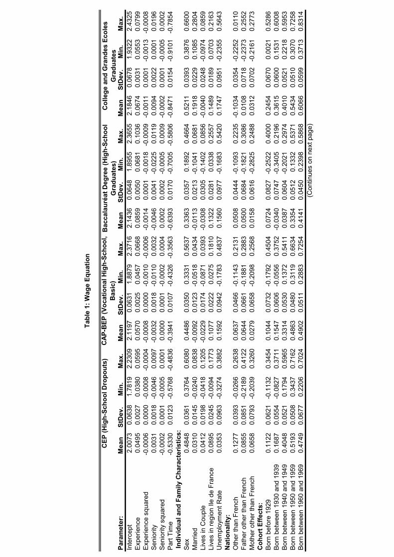
comparable to High-School dropouts in the United States. Table 1 presents estimation results for the wage

equation for each education group. Table 2 presents estimation results for the participation equation, once

again for each education group. Table 3 presents estimation results for the inter-firm mobility equations for the

four education groups. Table 4 presents estimation results for the initial conditions equations, and Table 5 gives

our estimates of the variance-covariance matrices for the individual effects (across the five equations) and for

the idiosyncratic effects (across the three main equations).

Wage Equation: Since estimating returns to seniority is one of the main motivations for adopting the joint

system estimation strategy, we first see that the returns are small,0.3% per year (in the first years). Returns to

experience are ten times larger than returns to tenure. Results of Table 1 show that the timing of the mobilities

in a career barely matters. More precisely, for the CEP category, each switch of job adds approximately65% to

the wage. However, one must add to the constant a component proportional to seniority and experience at exit

of the last job. But virtually none of these coefficients are significantly different from zero. Early moves in the

career are not good and moves after long stays in a job are marginally detrimental.

In this first table, two more facts are worthy of notice. First, and confirming results by Abowd, Kramarz,

Lengermann, and Roux (2004), interindustry wage differences are relatively compressed (when compared with

groups with a higher level of education), a consequence of minimum wages for a category that includes many

workers at the bottom of the wage distribution. Second, when correcting for mobility and participation, low-

education foreigners are better paid than nationals.

Participation and Mobility Equations: Tables 2 and 3 present our estimates of the participation and mo-

bility equations respectively, for CEP workers. Table 4 presents our estimates for the initial conditions, for the

same CEP workers. Most results are unsurprising. For instance, having low-age children lowers participation

but has no effect on mobility. More interesting are the coefficients on the lagged mobility and lagged partici-

pation. In contrast with most previous estimates, we are able to apportion state-dependence and heterogeneity.

Unsurprisingly, past participation and past mobility favors participation. More surprisingly though past mobil-

ity is associated with more mobility today. Therefore, workers are mobile both because some of them may be

high-mobility workers. But, lagged dependence is obviously a reflection of French labor market institutions

14

where workers often go from short-term contracts to short-term contracts, irrespective of their “tastes”. Unfor-

tunately, our data sources do not tell us the nature of the contract. Furthermore, this last result stands in sharp

contrast with those obtained by BFKT who estimate a negative sign, more in line with the free choice view of

mobility. Furthermore, seniority affects positively mobility, in contrast to what is found in BFKT for this group.

Stochastic Components:Table 5 presents estimates of variance-covariance components of the individual

effects for our five equations in the first panel and of the residuals of the three main equations in the second

panel. The results clearly show that those who participate are also relatively high-wage workers (both in terms

of individual effects and in terms of error term).

5.3 Results for CAP-BEP holders (Vocational Technical School, basic)

One element that distinguishes continental education systems, the French as well as the German, is the existence

of well-developed apprenticeship training. Indeed, this feature is well-known for Germany but it is also quite

important in France. Students who obtain the CAP (Certificat d’Aptitude Professionnelle) or the BEP (Brevet

d’Enseignement Professionnel) have spent part of their education in firms and the rest within schools where

they were taught both general and vocational subjects. It has no real equivalent in the US system.

Wage Equation: Returns to tenure, presented in Table 1, for workers with a vocational technical education

are negative, almost significantly so. We believe that negative returns are not only possible but confirmed by

many features of the French labor market, as well as other empirical evidence that we discuss now. Most

important to understand this feature is theJW function. Results are indeed very similar to those obtained

for high-school dropouts. In particular, job changes always entail a large wage gain, roughly equal to 65%,

unrelated to the seniority at the moment of the change. However, and in contrast with dropouts, a move very

early in the career has a small negative effect (-0.5%) and more significant, a move late in a career within a

firm. Indeed, moves after more than 10 years of seniority generate a wage loss of more than -2% per year of

seniority which is not compensated by the 1.3% increase per year of experience.

Participation and Mobility Equations: The estimated coefficients for the participation equation are very

similar to those obtained for the previous group. More interestingly, and related to the wage equation, we

find no evidence of lagged dependence in mobility. However, mobility is only mildly related to seniority

(more seniority inducing less mobility). Hence, workers appear to move at virtually all tenures, because they

lose nothing – on the contrary – by doing so, with one exception though for very long tenures. Notice also

that having young children affects strongly both participation and initial participation equation, in contrast to

college-educated groups.

Stochastic Components:For this group, most components are not significantly different from zero. Only

15

participation and wage person effects are positively correlated. In contrast, the same correlation is negative,

significantly so but mildly, for the idiosyncratic error terms.

5.4 Results for Baccalauréat Holders (High-School Graduates)

High-school graduation in France means that students have succeeded in a national exam, called the Baccalau-

réat. It is a passport to higher education, even though not all holders of the Baccalauréat go to a University.

And, furthermore, since many students who attend university never obtain a degree the group here potentially

includes workers who never completed any degree in the higher education system.

Wage Equation: Indeed, results for this group, presented again in Table 1, are very similar to those given

for the CEP holders. Returns to experience are large but returns to seniority are essentially zero. However,

the estimates for theJW function are very striking. First, there is a clear decrease in returns to mobility

when comparing short job spells and long job spells. In particular, mobility after ten years in a job brings

approximately a 35% bonus when mobility after up to 5 years in a job appears to add 100%. In addition, the

component proportional to seniority is very negative for the long job spells, destroying 3.5% per year. Hence,

a mobility after ten years in a job generates an average loss of at least 35% of the wage in comparison with

mobilities at shorter tenures. Notice though that the component proportional to experience is increasing with

experience and partly compensate for these relative losses.

Participation and Mobility Equations: Most results are very consistent with those obtained previously

for the CEP holders (all in Tables 2 and 3) . Interestingly though, the positive lagged dependence of mobility

disappears and even becomes marginally negative, a result that is consistent with results for the US. In contrast

to results obtained for CEP holders, the seniority coefficient in the mobility equation is not significantly different

from zero. Hence, the Baccalauréat group is quite special in that display no clear pattern of mobility within a

job, a potential reflection that careers where affected by involuntary job losses, at long tenures.

Stochastic Components:For workers in this category, central are the positive correlations between the

participation and the wage equations that come both from individual effects and from idiosyncratic terms. But

high-wage individuals are low-mobility workers. In addition, the participation and mobility idiosyncratic error

terms are highly positively correlated, another proof that non-participation (non-employment) and mobility are

negatively associated.

16

5.5 Results for University and Grandes Ecoles Graduates

Another element that distinguishes the French education system from other continental education systems as

well as from the American system is the existence of a very selective set of so-called Grandes Ecoles that work

in parallel with Universities. The former system delivers masters degrees mostly in engineering and in business.

It is very selective, in contrast to the rest of higher education.

Wage Equation: Interestingly, results for the group of graduates stand in sharp contrast with those obtained

for the other education groups (see Table 1). Not because returns to experience differ but mostly because returns

to seniority are now sizeable, approximately1% per additional year.6 Furthermore, the estimatedJW function

is also specific to that group. More precisely, wage gains not only come from the number of job changes but

also from the timing of these changes. Optimally, job changes after at most 5 years in that job are those most

profitable since they add4.5% per year of seniority to the starting point of the new job. Hence, say after 5 years

in a job, a graduate worker loses from the lost seniority (5%) but gains from the move (approximately80%)

and from the moment of the move (23%) and may lose something if the move was made too early in the career.

Notice that any move made later in the career, i.e. after 5 years of experience entails no loss nor gain due to

experience.

Other interesting facts must be noted for this group of graduates. First, working part-time entails much

bigger losses than for other groups. Furthermore, sizeable inter-industry wage differences can be found. As

mentioned above, such results are perfectly in line with those estimated by Abowd, Kramarz, Lengermann, and

Roux (2004) in their comparison of France and the United States. Wage differences mostly come from the

upper part of the wage distribution. Finally, for all other education groups, foreigners were better compensated

than nationals. Here, this is the contrary. Getting a higher education may be a solution to employment problems

for those born abroad (Maghreb, Portugal,...). But, even though we can not use the word discrimination, pay is

lower potentially reflecting a limited access to the Grandes Ecoles, the most selective and high-paying education

within this graduate group.

Participation and Mobility Equations: Mobility for this group displays no lagged dependence. Further-

more, workers’ mobility is virtually not related to seniority. And there is no relation between mobility and

experience; evidence that engineers and professionals careers entail job changes at all ages. In the participation

equation, the relatively large coefficient on the lagged participation indicator is a reflection of the labor market

orientation of those endowed with a higher graduate education. Furthermore, and in contrast to all other groups,

participation choices are not affected by having young children. Indeed, this very educated group obviously

6(Results for the group of University Technical University undergraduates are very similar to those presented in this subsection.Hence we do not report them.

17

selected their education because they wanted to work (remember that participation is, in fact, employment).

Stochastic Components:As found before, high-participation individuals are also high-wage individuals,

but this much less so than for other groups, another reflection that the choice of a high-level education signals

a high willingness to work and, indeed, to find a job. And, individuals faced with a positive idiosyncratic wage

shock are also faced with a positive mobility shock.

6 A Comparison with the United States

6.1 Facts

In this subsection, we compare our results with those obtained by BFKT for the United States using exactly

the same model specification with two initial equations for mobility and participation, with three equations for

wage, mobility and participation, the last two including lagged dependence. In addition, the same stochastic

assumptions were made, that is the error terms were the sum of an individual effect (one for each of the five

equations, all potentially correlated) and an idiosyncratic term for the three main equations (all potentially

correlated). The model was estimated for three education groups: high-school dropouts, high-school graduates,

and college graduates. The PSID was used for estimation. Some variables included in BFKT were not available

in the panel that we use, in particular race. We present a comparison of the estimates for a subset of the

parameters that we believe are the most telling and important. Estimates for the College Educated group are

presented in Table 6 whereas estimates for High-School Dropouts are presented in Table 7.

The first difference to be noted is essentially in the estimated returns to seniority. They are large in the

United States and small in France. We discuss this fact in the next subsection extensively. Related to this, we

see that returns to experience are slightly larger in France than in the United States for the two groups. But the

total of returns to experience and returns to seniority is much larger in the U.S.. Indeed, when considering how

wages behave after job mobility, we have to compare the estimatedJW functions. Here again, some differences

stand out. First, the part proportional to the number job to job switches appear to be better compensated in

France than in the U.S.; in particular, those movements out of jobs that lasted at most 5 years. Whereas in the

United States, movements out of jobs that lasted more than 10 years are much better compensated than other

movements. Notice the similarities across countries in the part of theJW function proportional to seniority

for the college educated: movements exactly after 5 years in a job appear to be most profitable. However,

for the high-school dropouts, movements after very long periods in a job are better rewarded in the United

States whereas movements before 6 years in a job appear to be (marginally) better in France for this category.

To summarize, short spells appear to be (slightly) the most profitable in France, the reverse being true in the

18

United States.

Other facts on wages are worthy of notice. We already mentioned some of them in our discussion of the

French results. In particular, inter-industry wage differentials are less compressed in the top part of the wage

distribution in France but are large in every education group in the United States.

Related to differences on wage determination that we just described, differences in the mobility processes

between France and the United States must be stressed. First, in the United States, the mobility process always

displays negative lagged dependence; after a move a worker tends to stay at the next period. This is not true

in France. First, for the college educated workers there is no state dependence in the mobility process. But,

more striking, there is positive state dependence in the mobility process for the CEP holders. Hence, a worker

who just moved is more likely to move again, a consequence, as noted above, of repeated employment of low-

education workers in sequences of short-term contracts. However, in the United States, workers tend to move

early in a job (negative sign on the seniority coefficient in the mobility equation); a feature of the American

labor market. But, this is not so for the two education groups in France where the CEP holders tend to move

more often at longer tenures (and mildly so for the college-educated).

Finally, the comparison of the variance-covariance matrices of individual effects and of the variance-

covariance matrices of idiosyncratic effects across the two countries confirms previous findings. First, the

U.S. data source (the PSID) because of its survey structure captures initial conditions much better than the

French data source (the DADS-EDP, of administrative origin). In particular the former has much better initial

variables whereas imputations had to be performed in 1976 for the latter. Second, concentrating on the correla-

tion of individual effects in the three main equations, participation and wage are highly positively correlated in

both countries. But, when mobility equation is involved, signs are similar in the two countries for both groups

of education but the estimates are imprecise in France. Finally, high-mobility individuals are clearly low-wage

and low-participation individuals in the United States, stressing again the different role played by mobility in

the two countries.

6.2 Returns to Seniority as an “Incentive Device”?

A natural question arising from the above comparison can be formulated as follows. Are the different features

that seem to prevail in each country related ? Or, put differently, are the small estimated returns to seniority

in France related to the patterns of mobility as estimated above, in particular to the relatively low job-to-job

transition rates, as well to the relatively high risk of losing one’s job ? Whereas, in the United States, are

the large estimated returns to seniority related to this country patterns of mobility as estimated in BFKT and

discussed just above, in particular the relatively high job-to-job transition rates, the low unemployment rate and

19

the relatively high probability of exit out of unemployment ?

In this subsection, we show that these features are indeed part of a system. An equilibrium search model

with wage-tenure contracts is shown to be a good tool for understanding and summarizing this system . The

properties of the wage profiles at the stationary equilibrium are contrasted using the respective characteristics

of the two labor markets.

The characteristics that matter for both our estimates and this model are the following. In France, the

unemployment rate is muc larger than in the US (9.4% vs. 5,7% in March 2004 according to OECD data

sources). Consequently, the job offer arrival rate can be assumed to be larger in the US than in France. Indeed,

Jolivet, Postel-Vinay and Robin (2004), using a job search model, have estimated the job arrival rates for the

US (PSID, 1993-1996) and several European countries (ECHP, 1994-2001). The estimated job arrival rate is

more than three times larger on the US labor market than on the French one (1.7114 per annum vs. 0.5614).

The job search model used in this endeavor was developed recently by Burdett and Coles (2003). In particu-

lar, this model generates an unique equilibrium wage-tenure contract. We show that this wage-tenure contract is

such that the slope of the wage function with respect to job tenure, for the first months or years, is an increasing

function of the job offer arrival rate. Hence, it is an increasing function of the realized mobility on the labor

market.

We start by summarizing the important aspects of the model. In Burdett and Coles (2003), the individuals

are risk adverse. Letλ denote the job offers arrival rate andδ is the arrival rate of new workers into the

labor force and the outflow rate of workers out from the labor market. Letp denote the instantaneous revenue

received by firms for each worker employed andb is the instantaneous benefit received by each unemployed

worker (p > b > 0).

The equilibrium is unique and is such that the optimal wage-tenure contract selected by a firm offering the

lower starting wage satisfies

(19)dw

d t=

δ√p− w2

p− w

u′(w)

∫ w2

w

u′(s)√p− s

d s

with the initial conditionw(0) = w1 and wherew1, w2 are such that

(20)

(δ

λ + δ

)2

=p− w2

p− w1,

(21) u(w1) = u(b)−√

p− w1

2

∫ w2

w1

u′(s)√p− s

d s,

20

where[w1;w2] is the support of the distribution of wages paid by the firms (w1 < b andw2 < p).

Let us assume that the utility function is CRRA,u(w) = w1−σ

1−σ (σ > 0). Burdett and Coles (2003) show

that the optimal wage-tenure contract, namely the baseline salary contract, is such that there exists a tenure such

that, from this tenure on, this (baseline salary) contract is identical to the contract offered by a high-wage firm

with a higher entry wage.

(22)d2 w

d t2=

(dw

d t

)2 1p− w

[σ p

w− (σ + 1)

]− δ

√p− w√p− w2

dw

d t

with the initial conditionsw(0) = w1 and

(23)dw(0)

d t=

δ√p− w2

p− w1

u′(w1)

∫ w2

w1

u′(s)√p− s

d s

The differential equation22 is highly non linear and have to be solved numerically. This can done by setting

(λ, δ, σ, p) to some values and using, for instance, the procedure NDSolve of Mathematica.

In order to study the behavior of the wage-tenure contract curve with respect to the values of the job offers

arrival rate, we have used the same parameter values as Burdett and Coles (see their section 5.2). Hence, we have

setp = 5, δλ = 0.1 andb = 4.6. For each value of the relative risk aversion coefficient (σ ∈ 0.2, 0.4, 0.8, 1.4),

we solve the system of equations(22)-(23) numerically for a set a values of the job offers arrival rate. The

results are depicted in Figure6.2 for σ = 0.2, in Figure6.2 for σ = 0.4, in Figure6.2 for σ = 0.8 and in Figure

6.2 for σ = 1.4. The Figures present these wage contract curves for the first 10 years of seniority. For all values

of the relative risk aversion coefficient, we see that wage increases much more rapidly, in particular during the

first year, for larger job offers arrival rates.

Using the values of the job offers arrival rates (per year) estimated by Jolivet, Postel-Vinay and Robin

(2004) for France and the US, the U.S. situation corresponds to the curve whereλ = 0.005 and the French

labor market to the curve whereλ = 0.001. And, for all relative risk aversion coefficients, the equilibrium

wage-tenure contract curves are such that the high mobility country (the United States) has much higher returns

to seniority than the low mobility country (France).

Two points are worth mentioning at this stage. First, we take - as firms appear to be doing - institutions that

affect mobility as given. For instance, the housing market is much more fluid in the United States than in France

(because, for instance, of strong regulations and transaction costs). Or, subsidies and government interventions

preventing firm to go bankrupt seem more prevalent in France, dampening the forces of “creative destruction

21

”in this country. And firms must react within this environment. Therefore, French firms face a workforce

that is mostly stable with little incentives to move, even after an involuntary separation. Second, as a recent

paper by Wasmer argues (Wasmer, 2003), it is likely that French firms will invest in firm-specific human capital

for this exact reason. In contrast, American firms face a workforce that is very mobile. Therefore, following

again Wasmer (2003), these firms should rely on general human capital. Now, does it mean that returns to

seniority should be large in France and small in the United States ? Or, put differently, should French firms

pay for something they get “by construction” (of the institutions). This is, we believe, the misconception that

has plagued some of this research in the recent years. And, the above model gets it right. The optimal tenure

contract when mobility is strong should be larger than when mobility is weak.

22

0 500 1000 1500 2000 2500 3000 3500tenure

1

2

3

4

5

wage

Wage function of tenure in days Sigma equal to 0.2

lambda>=0.01

lambda=0.005

lambda=0.002

lambda=0.001

lambda=0.0001

lambda=0.00005

0 500 1000 1500 2000 2500 3000 3500tenure

1.5

2

2.5

3

3.5

4

4.5

5

wage

Wage function of tenure in days Sigma equal to 0.4

lambda>=0.01

lambda=0.005

lambda=0.002

lambda=0.001

lambda=0.0001

lambda=0.00005

0 500 1000 1500 2000 2500 3000 3500tenure

2.5

3

3.5

4

4.5

5

wage

Wage function of tenure in days Sigma equal to 0.8

lambda>=0.01

lambda=0.005

lambda=0.002

lambda=0.001

lambda=0.0001

lambda=0.00005

0 500 1000 1500 2000 2500 3000 3500tenure

3

3.5

4

4.5

5

wage

Wage function of tenure in days for sigma equal to 1.4

lambda>=0.01

lambda=0.005

lambda=0.002

lambda=0.001

lambda=0.0001

lambda=0.00005

23

7 Conclusion

In this article, we estimated returns to seniority in a structural framework in which participation, mobility and

wages are jointly modelled. We include both state-dependence and unobserved correlated individual hetero-

geneity in the decisions. To estimate this complex structure, we use Bayesian techniques. The model is esti-

mated using French longitudinal data sources for the period 1976-1995. Results presented for four groups of

education show that returns to seniority are virtually zero, potentially negative for some low-education groups,

slightly positive for college-educated workers (1% per year of seniority). A comparison with results obtained

for the United States by BFKT using the exact same specification and similar estimation techniques (on the

PSID) shows that returns to seniority are much lower in France and that returns to experience are virtually

identical. Furthermore, unreported results (available from the authors) show that OLS estimates of the returns

to seniority are much higher than those obtained for our system of equations. In addition, the same unreported

results demonstrate that instrumental variables estimation following exactly Altonji’s suggestions give results

that look relatively similar to those obtained for our system of equations. Estimates are always lower than those

obtained with OLS. However, Altonji’s IV technique gives sometimes slightly higher estimates than those we

obtain for our system (low education groups) and sometimes slightly lower estimates than those we obtain for

our system (college-educated workers). This comparison for France stands in sharp contrast with that for the

United States; results in BFKT show that Altonji’s technique yields much lower returns to seniority than those

obtained for the system of equations. Still, using Altonji’s technique in both countries, our result still holds:

returns to seniority are lower in France than in the United States.

Hence, modelling jointly mobility and participation with wages has non-trivial consequences that may

vary across countries. In particular, the labor market institutions and state (high unemployment versus low

unemployment, among other things) or other market institutions such as the housing market that may favor

or discourage mobility are likely to have far-reaching effects on these mobility and participation processes.

Techniques that do not deal directly with these questions are likely to give incomplete answers.

8 Bibliography

Abraham K.G. and H.S. Farber (1987), “Job Duration, Seniority, and Earnings”,American Economic Review,

vol. 77, 3, 278-297.

Abowd J. M., Kramarz F. and D. N. Margolis (1999), “High Wage Workers and High Wage Firms”,Economet-

rica, 67, 251-334.

24

Altonji J. G. and R. A. Shakotko (1987), “Do Wages Rise With Job Seniority ?”,Review of Economic Studies,

LIV, 437-459.

Altonji J. G. and N. Williams (1992), “The Effects of Labor Market Experience, Job Seniority and Job Mobility

on Wage Growth”, NBER Working Paper Series 4133.

Altonji J. G. and N. Williams (1997), “Do Wages Rise With Job Seniority ? A Reassessment”, NBER Working

Paper Series 6010.

Becker G.S. (1964),Human Capital, Columbia Press.

Buchinsky M., Fougère D., Kramarz F. and R. Tchernis (2002), “Interfirm Mobility, Wages, and the Returns to

Seniority and Experience in the U.S.”, CREST Working Papers 2002-29, Paris.

Burdett K. and M. Coles (2003), “Equilibrium Wage-Tenure Contracts”,Econometrica, vol. 71, 5, 1377-1404.

Flinn Ch. J. (1986), “Wages and Job Mobility of Young Workers”,Journal of Political Economy, 94, S88-S110.

Heckman J. J. (1981), “Heterogeneity and State Dependence”, inStudies in Labor Market, Rosen S. ed., Uni-

versity of Chicago Press.

Hyslop D. R. (1999), “State Dependence, Serial Correlation and Heterogeneity in Intertemporal Labor Force

Participation of Married Women”,Econometrica, 67, 1255-1294.

Jolivet G., Postel-Vinay F. and J.-M. Robin (2004), “The Empirical Content of the Job Search Model: Labor

Mobility and Wage Distributions in Europe and the US”, Mimeo Crest, Paris.

Jovanovic B. (1979), “Firm-specific Capital and Turnover”,Journal of Political Economy, vol. 87, 6, 1246-

1260.

Jovanovic B. (1984), “Matching, Turnover, and Unemployment”,Journal of Political Economy, vol. 92, 1,

108-122.

Lazear E. P. (1979), “Why is there mandatory retirement ?”,Journal of Political Economy, vol. 87, 6, 1261-

1284.

Lazear E. P. (1981), “Agency, earnings profiles, productivity and hours restrictions”,American Economic Re-

view, vol. 71, 4, 606-620.

Lazear E. P. (1999), “Personnel Economics: Past Lessons and Future Directions. Presidential Address to the

Society of Labor Economics, San Francisco, May 1, 1998.”,Journal of Labor Economics, vol.17, 2, 199-236.

25

Lillard L. A. and R. J. Willis (1978), “Dynamic Aspects of Earnings Mobility”,Econometrica, 46, 985-1012.

Miller R.A. (1984), “Job Matching and Occupational Choice”,Journal of Political Economy, vol. 92, 6, 1086-

1120.

Mincer J. (1974), “Progress in Human Capital Analysis of the distribution of earnings”, NBER Working Paper

53.

Postel-Vinay F. and J.M. Robin (2002), “Equilibrium Wage Dispersion with Worker and Employer Heterogene-

ity”, Econometrica, 70, 2295-2350.

Salop J. and S. Salop (1976), “Self-Selection and Turnover in the Labor Market”,Quarterly Journal of Eco-

nomics, 90, 619-627.

Topel R. H. (1991), “Specific Capital, Mobility, and Wages: Wages Rise with Job Seniority”,Journal of Politi-

cal Economy, 99, 145-175.

Wasmer E. (2003), “Interpreting Europe and US labor markets differences : the specificity of human capital

investments”, CEPR discussion paper 3780.

A Mobility equation

A.1 Parameterγ

This parameter entersmmit∗ for t = 2, ..., T − 1

mmit∗ = γmit−1 + XMit δM + ΩI

i θM,I

If we put apart this term in the full conditional likelihood, we get:

N∏

i=1

T−1∏

t=2

exp(− yit

2V m(m∗

it −Mmit )2

)= exp

(− 1

2V m

N∑

i=1

(m∗i

2,T−1 − Mmi

2,T−1)′(m∗

i

2,T−1 − Mmi

2,T−1)

)

= exp

(− 1

2V m

N∑

i=1

(Ai

2,T−1 − γLmi

2,T−1)′(Ai

2,T−1 − γLmi

2,T−1)

)

with:

26

• Mmit = mm∗

it+

ρy,m − ρw,mρy,w

1− ρ2y,w︸ ︷︷ ︸

a

(y∗it −my∗it) +ρw,m − ρy,mρy,w

σ(1− ρ2y,w)︸ ︷︷ ︸

b

(wit −mwit)

• m∗i

2,T−1=

yi2m∗i2

...

yiT−1m∗iT−1

• Mmi

2,T−1=

yi2Mmi2

...

yiT−1MmiT−1

• Ait = m∗it −Mm

it + γmit−1 = m∗it −XM

it δM − ΩIi θ

I,M − a(y∗it −my∗it)− b(wit −mwit)

By gathering squared and crossed terms, we get:

V post,−1γ = V prior,−1

γ +1

V m

N∑

i=1

(Lmi

2,T−1)′

Lmi

2,T−1

V post,−1γ Mpost

γ = V prior,−1γ Mprior

γ +1

V m

N∑

i=1

(Lmi

2,T−1)′

Ai

2,T−1

A.2 ParameterδM

We proceed the same way as before and we get with analogous notations:

V post,−1δM = V prior,−1

δM +1

V m

N∑

i=1

(XM

i

2,T−1)′

XMi

2,T−1

V post,−1δM Mpost

δM = V prior,−1δM Mprior

δM +1

V m

N∑

i=1

(XM

i

2,T−1)′

Ai

2,T−1

with Ait = m∗it −Mm

it + δMXMit = m∗

it − γmit−1 − ΩIi θ

I,M − a(y∗it −my∗it)− b(wit −mwit)

B Wage equation

B.1 ParameterδW

We have to take into account thatδW enters bothmwit for t = 1...T andMmit for t = 1...T − 1.

27

Thus if we put apart these terms in the full conditional likelihood, we get:

N∏

i=1

exp

(− 1

2V w

T∑

t=1

yit(wit −Mwit )

2

)exp

(− 1

2V m

T−1∑

t=1

yit(m∗it −Mm

it )2)

=N∏

i=1

exp

(− 1

2V w

T∑

t=1

yit(Ait −XWit δW )2

)exp

(− 1

2V m

T−1∑

t=1

yit(Bit + bXWit δW )2

)

with:

• wit −Mwit = Ait −XW

it δW

• m∗it −Mm

it = Bit + bXWit δW

which is equivalent to:

• Ait = wit − ΩIi θ

I,W − ρy,wσ(y∗it −my∗it))

• Bit = m∗it −mm∗

it− a(y∗it −my∗it)− b(wit − ΩI

i θI,W )

If we use analogous notations as before, we get:

V post,−1δW = V prior,−1

δW +1

V w

N∑

i=1

(XW

i

1,T)′

XWi

1,T

+b2

V m

N∑

i=1

(XW

i

1,T−1)′

XWi

1,T−1

V post,−1δW Mpost

δW = V prior,−1δW Mprior

δW +1

V w

N∑

i=1

(XW

i

1,T)′

Ai

1,T − b

V m

N∑

i=1

(XW

i

1,T−1)′

Bi

1,T−1

C Participation equation

C.1 ParameterγY

We have to take into account thatγY enters bothmy∗it for t = 2...T , Mwit for t = 2...T andMm

it for t = 2...T−1

Thus if we put apart these terms in the full conditional likelihood, we get:

N∏

i=1

exp

(−1

2

T∑

t=2

(y∗it −my∗it)2 − 1

2V w

T∑

t=2

yit(wit −Mwit )

2 − 12V m

T−1∑

t=2

yit(m∗it −Mm

it )2)

=N∏

i=1

exp

(−1

2

T∑

t=2

(Ait − γY Lyit)2 − 12V w

T∑

t=2

yit(Bit + ρy,wσγY Lyit)2 − 12V m

T−1∑

t=2

yit(Cit + aγY Lyit)2)

28

with:

• y∗it −my∗it = Ait − γY Lyit

• wit −Mwit = Bit + ρy,wσγY Lyit

• m∗it −Mm

it = Cit + aγY Lyit

which is equivalent to:

• Ait = y∗it − γMLmit −XYit δY − ΩI

i θI,Y

• Bit = wit −mwit − ρy,wσAit

• Cit = m∗it −mm∗

it− b(wit −mwit)− aAit

If we use analogous notations as before, we get:V

post,−1γY

= Vprior,−1γY

+N∑

i=1

(Ly

2,Ti

)′Ly

2,Ti

+ρ2

y,wσ2

V w

N∑

i=1

(Ly

i

2,T)′

Lyi

2,T+

a2

V m

N∑

i=1

(Ly

i

2,T−1)′Ly

i

2,T−1

Vpost,−1γY

Mpost

γY= V

prior,−1γY

Mprior

γY+

N∑

i=1

(Ly

2,Ti

)′A

2,Ti − ρy,wσ

V w

N∑

i=1

(Ly

i

2,T)′

Bi2,T − a

V m

N∑

i=1

(Ly

i

2,T−1)′Ci

2,T−1

C.2 ParameterγM

We proceed the same way and we get:V

post,−1γM

= Vprior,−1γM

+N∑

i=1

(Lm

2,Ti

)′Lm

2,Ti +

ρ2y,wσ2

V w

N∑

i=1

(Lmi

2,T)′

Lmi2,T

+a2

V m

N∑

i=1

(Lmi

2,T−1)′Lmi

2,T−1

Vpost,−1γM

Mpost

γM= V

prior,−1γM

Mprior

γM+

N∑

i=1

(Lm

2,Ti

)′A

2,Ti − ρy,wσ

V w

N∑

i=1

(Lmi

2,T)′

Bi2,T − a

V m

N∑

i=1

(Lmi

2,T−1)′Ci

2,T−1

with:

• Ait = y∗it − γY Lyit −XYit δY − ΩI

i θI,Y

• Bit = wit −mwit − ρy,wσ (Ait)

• Cit = m∗it −mm∗

it− b(wit −mwit)− a (Ait)

C.3 ParameterδY

We proceed the same way and we get:

29

Vpost,−1δY

= Vprior,−1δY

+N∑

i=1

(X

Yi

2,T)′

XYi

2,T+

ρ2y,wσ2

V w

N∑

i=1

(XY

i

2,T)′

XYi

2,T+

a2

V m

N∑

i=1

(XY

i

2,T−1)′

XYi

2,T−1

Vpost,−1δY

Mpost

δY= V

prior,−1δY

Mprior

δY+

N∑

i=1

(X

Yi

2,T)′

A2,Ti − ρy,wσ

V w

N∑

i=1

(XY

i

2,T)′

Bi2,T − a

V m

N∑

i=1

(XY

i

2,T−1)′

Ci2,T−1

with:

• Ait = y∗it − γY Lyit − γMLmit − ΩIi θ

I,Y

• Bit = wit −mwit − ρy,wσ (Ait)

• Cit = m∗it −mm∗

it− b(wit −mwit)− a (Ait)

D Initial equations

D.1 ParameterδM0

δM0 only entersm∗

i1. We thus get:

V post,−1

δM0

= V prior,−1

δM0

+1

V m

N∑

i=1

(XM

i1

)′XM

i1

V post,−1

δM0

Mpost

δM0

= V prior,−1

δM0

Mprior

δM0

+1

V m

N∑

i=1

(XM

i1

)′Ai1

with:

• Ai1 = m∗i1 − ΩI

i αI,M − a(y∗i1 −my∗i1)− b(wi1 −mwi1)

D.2 ParameterδY0

We proceed the same way and we get:

V post,−1

δY0

= V prior,−1

δY0

+N∑

i=1

XYi1′XY

i1 +

(ρ2

y,wσ2

V w+

a2

V m

)N∑

i=1

XYi1

′XY

i1

V post,−1

δY0

Mpost

δY0

= V prior,−1

δY0

Mprior

δY0

+N∑

i=1

XYi1′Ai −

N∑

i=1

XYi1

′ (ρy,wσ

V wBi +

a

V mCi

)

30

with:

• Ai = y∗i1 − ΩEi αI,Y

• Bi = wi1 −mwi1 − ρy,wσAi

• Ci = m∗i1 −mm∗

i1− b(wi1 −mwi1)− aAi

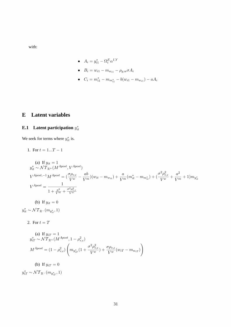
E Latent variables

E.1 Latent participation y∗it

We seek for terms wherey∗it is.

1. For t = 1...T − 1

(a) If yit = 1y∗it ∼ NT R+(MApost, V Apost)

V Apost,−1MApost = (σρv,ε

V w− ab

V m)(wit −mwit) +

a

V m(m∗

it −mm∗it) + (

σ2ρ2v,ε

V w+

a2

V m+ 1)my∗it

V Apost =1

1 + a2

V m + σ2ρ2v,ε

V w

(b) If yit = 0

y∗it ∼ NT R−(my∗it , 1)

2. For t = T

(a) If yiT = 1y∗iT ∼ NT R+(MApost, 1− ρ2

v,ε)

MApost = (1− ρ2v,ε)

(my∗iT (1 +

σ2ρ2v,ε

V w) +

σρv,ε

V w(wiT −mwiT )

)

(b) If yiT = 0

y∗iT ∼ NT R−(my∗iT , 1)

31

E.2 Latent mobility m∗it

Two conditions must be checked: first,t = 1...T − 1 and,yit = 1. When these conditions are fulfilled, we

distinguish between different cases:

1. If yit+1 = 0

m∗it ∼ N (Mm

it , V m) and mit = I(m∗it > 0)

2. If yit+1 = 1

(a) If mit = 1

m∗it ∼ NT R+(Mm

it , V m)

(b) If mit = 0

m∗it ∼ NT R−(Mm

it , V m)

F Variance-Covariance Matrix of Residuals

We use the Hastings-Metropolis algorithm because our priors are not conjugate (the posterior does not belong

to the same family of distributions as the prior).

G Variance-Covariance Matrices of Individual EffectsΣIi |(...); z; y, w

The parametersηj , j = 1...10 andγj , j = 1...5 do not enter the full conditional likelihood. They only enter the

prior distributions. Let us denotep the parameter we are interested in amongηj , j = 1...10 andγj , j = 1...5.

l(p|(−p), θI) = l(θI |p)π0(p)

= π0(p)N∏

i=1

l(θIi |ΣI

i (p))

∝ π0(p)N∏

i=1

1√det(ΣI

i (p))exp

(−1

2θIi′ΣI,−1

i (p)θIi

)

We face non conjugate distributions therefore we use the independent Hastings-Metropolis algorithm with

the prior distribution as instrumental distribution.

32

?

H Individual effects

The likelihood terms that includeθI writes as:

N∏

i=1

exp(−1

2(y∗i1 −my∗i1)

2

)exp

(− yi1

2V w(wi1 −Mw

i1)2)

T∏

t=2

exp(−1

2(y∗it −my∗it)

2

)exp

(− yit

2V w(wit −Mw

it )2)

exp(−yit−1

2V m(m∗

it−1 −Mmit−1)

2)

with

Mmit = mm∗

it+ a(y∗it −my∗it) + b(wit −mwit)

Mwit = mwit + σρv,ε(y∗it −my∗it)

The following notations are useful:

1. First term

(y∗i1 −my∗i1)2 = (Ai1 − ΩI

i αI,Y )2

Ai1 = y∗i1 −XYi1δY0

2. Second term

yi1(wi1 −Mwi1)2 = yi1(Bi1 − ΩI

i θI,W + ρv,εσΩI

i αI,Y )2

Bi1 = wi1 −XWi1δw − ρv,εσ(y∗i1 −XYi1δ

Y0 )

Bi1 = yi1Bi1

ΩIi1 = yi1ΩI

i

33

3. Third term

(y∗it −my∗it)2 = (Cit − ΩI

i θY,I)2

Cit = y∗it −XYitδY − γY yit−1 − γMmit−1

4. Fourth term

yit(wit −Mwit)2 = yit(Dit − ΩI

i θW,I + ρv,εσΩI

i θY,I)2

Dit = wit −XWitδw − ρv,εσCit

Dit = yitDit

ΩIit = yitΩI

i

5. Fifth term

For t > 1

yit(m∗it −Mm∗

it)2 = yit(Fit + ΩI

i (−θM,I + aθY,I + bθW,I))2

Fit = m∗it − γmit−1 −XMitδ

M − aCit − b(wit −XWitδw

Fit = yitFit

For t = 1

yi1(m∗i1 −Mm∗

i1)2 = yi1(Gi1 + ΩI

i (−αM,I + aαY,I + bθW,I))2

Gi1 = m∗i1 −XMi1δ

M0 − aAi1 − b(wi1 −XWi1δ

w)

Gi1 = yi1Gi1

34

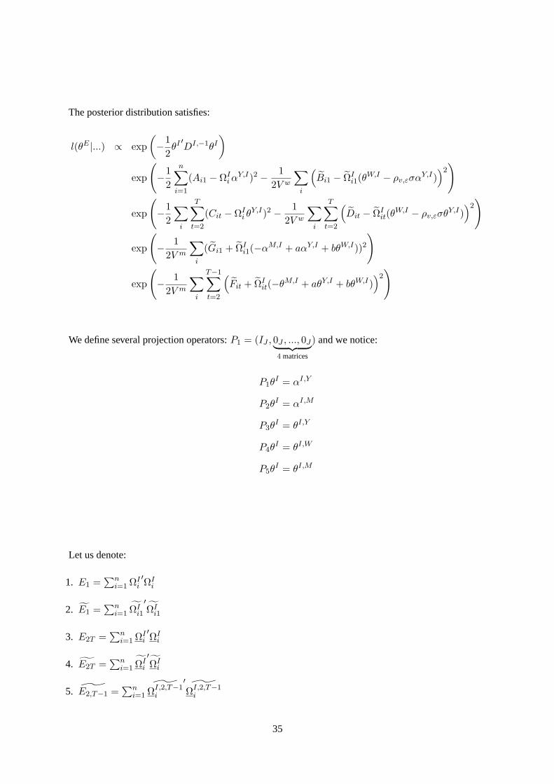
The posterior distribution satisfies:

l(θE |...) ∝ exp(−1

2θI ′DI,−1θI

)

exp

(−1

2

n∑

i=1

(Ai1 − ΩIi α

Y,I)2 − 12V w

∑

i

(Bi1 − ΩI

i1(θW,I − ρv,εσαY,I)

)2)

exp

(−1

2

∑

i

T∑

t=2

(Cit − ΩIi θ

Y,I)2 − 12V w

∑

i

T∑

t=2

(Dit − ΩI

it(θW,I − ρv,εσθY,I)

)2)

exp

(− 1

2V m

∑

i

(Gi1 + ΩIi1(−αM,I + aαY,I + bθW,I))2

)

exp

(− 1

2V m

∑

i

T−1∑

t=2

(Fit + ΩI

it(−θM,I + aθY,I + bθW,I))2

)

We define several projection operators:P1 = (IJ , 0J , ..., 0J︸ ︷︷ ︸4 matrices

) and we notice:

P1θI = αI,Y

P2θI = αI,M

P3θI = θI,Y

P4θI = θI,W

P5θI = θI,M

Let us denote:

1. E1 =∑n

i=1 ΩIi′ΩI

i

2. E1 =∑n

i=1 ΩIi1

′ΩI

i1

3. E2T =∑n

i=1 ΩIi′ΩI

i

4. E2T =∑n

i=1 ΩIi

′ΩI

i

5. E2,T−1 =∑n

i=1 ΩI,2,T−1i

′ΩI,2,T−1

i

35

So we get for the variance-covariance matrix:

V−1

= DE,−10 +

E1 + (ρ2

v,εσ2

V w + a2V m )E1 − a

V m E1 0 T41 0

− aV m E1

1V m E1 0 T42 0

0 0 E2T +ρ2

v,εσ2

V w E2,T + a2V m E2,T−1 T43 T53

(− ρv,εσ

V w + abV m )E1 − b

V m E1 − ρv,εσ

V w E2T + abV m E2T−1 E1( 1

V w + b2V m ) + 1

V w E2T + b2V m E2T−1 T54

0 0 − aV m E2T−1 − b

V m E2T−11

V m E2T−1

?

As for the posterior mean:

∑ni=1 ΩI

i′Ai1 − ρv,εσ

V w

∑ni=1 ΩI

i1

′Bi1 − a

V m

∑ni=1 ΩI

i1

′Gi1

1V m

∑ni=1 ΩI

i1

′Gi1

∑ni=1 ΩI

i′Ci − ρv,εσ

V w

∑ni=1 ΩI

i

′Di − a

V m

∑ni=1 ΩI

iT−1

′F iT−1

1V w

∑ni=1 ΩI

i1

′Bi1 + 1

V w

∑ni=1 ΩI

i

′Di − b

V m

∑ni=1 ΩI

i1

′Gi1 − b

V m

∑ni=1 ΩI

iT−1

′F iT−1

1V m

∑ni=1 ΩI

iT−1

′F iT−1

?

36

Para

met

er:

Mea

nSt

Dev

.M

in.

Max

.M

ean

StD

ev.

Min

.M

ax.

Mea

nSt

Dev

.M

in.

Max

.M

ean

StD

ev.

Min

.M

ax.

Inte

rcep

t 2.

0073

0.06

381.

7819

2.23

092.

1197

0.06

311.

8879

2.37

162.

1436

0.06

481.

8955

2.36

552.

1846

0.06

781.

9322

2.43

25E

xper

ienc

e 0.

0495

0.00

270.

0380

0.05

950.

0570

0.00

250.

0457

0.06

680.

0859

0.00

500.

0681

0.10

360.

0674

0.00

310.

0553

0.07

99E

xper

ienc

e sq

uare

d -0

.000

60.

0000

-0.0

008

-0.0

004

-0.0

008

0.00

00-0

.001

0-0

.000

6-0

.001

40.

0001

-0.0

018

-0.0

009

-0.0

011

0.00

01-0

.001

3-0

.000

8S

enio

rity

0.00

310.

0018

-0.0

046

0.00

97-0

.003

20.

0018

-0.0

110

0.00

32-0

.004

60.

0041

-0.0

225

0.01

190.

0094

0.00

220.

0001

0.01

96S

enio

rity

squa

red

-0.0

002

0.00

01-0

.000

50.

0001

0.00

000.

0001

-0.0

002

0.00

040.

0002

0.00

02-0

.000

50.

0009

-0.0

002

0.00

01-0

.000

50.

0002

Par

t Tim

e -0

.533

00.

0123

-0.5

768

-0.4

836

-0.3

941

0.01

07-0

.432

6-0

.356

3-0

.639

30.

0170

-0.7

005

-0.5

806

-0.8

471

0.01

54-0

.910

1-0

.785

4

Sex

0.48

480.

0361

0.37

640.

6080

0.44

860.

0350

0.33

310.

5637

0.33

630.

0357

0.18

920.

4664

0.52

110.

0393

0.38

760.

6600

Mar

ried

0.

0310

0.01

45-0

.024

00.

0838

-0.0

092

0.01

23-0

.051

80.

0434

-0.0

113

0.02

13-0

.104

10.

0681

0.19

180.

0229

0.10

850.

2804

Live

s in

Cou

ple

0.

0412

0.01

98-0

.041

80.

1205

-0.0

229

0.01

74-0

.087

10.

0393

-0.0

308

0.03

05-0

.140

20.

0856

-0.0

040

0.02

48-0

.097

40.

0859

Live

s in

regi

on Il

e de

Fra

nce

0.08

950.

0245

-0.0

094

0.17

730.

1077

0.02

220.

0275

0.18

100.

1322

0.02

810.

0338

0.25

570.

1489

0.01

890.

0703

0.21

63U

nem

ploy

men

t Rat

e0.

0353

0.09

63-0

.327

40.

3882

0.15

920.

0942

-0.1

783

0.48

370.

1560

0.09

77-0

.168

30.

5420

0.17

470.

0951

-0.2

355

0.56

43N

atio

nalit

y:O

ther

than

Fre

nch

0.12

770.

0393

-0.0

266

0.26

380.

0637

0.04

66-0

.114

30.

2131

0.05

080.

0444

-0.1

093

0.22

35-0

.103

40.

0354

-0.2

252

0.01

10Fa

ther

oth

er th

an F

renc

h 0.

0855

0.08

51-0

.218

90.

4122

0.06

440.

0661

-0.1

881

0.28

830.

0500

0.06

84-0

.182

10.

3086

0.01

080.

0718

-0.2

373

0.25

52M

othe

r oth

er th

an F

renc

h 0.

0658

0.07

93-0

.203

90.

3260

0.02

790.

0658

-0.2

098

0.25

680.

0158

0.06

16-0

.282

50.

2488

0.03

120.

0702

-0.2

161

0.27

73C

ohor

t Effe

cts:

Bor

n be

fore

192

9 0.

1122

0.06

21-0

.113

20.

3454

0.10

440.

0732

-0.1

792

0.45

040.

0724

0.08

27-0

.252

20.

4000

0.24

540.

0670

0.00

210.

5286

Bor

n be

twee

n 19

30 a

nd 1

939

0.16

870.

0554

-0.0

827

0.37

110.

1547

0.06

06-0

.055

60.

3752

-0.0

340

0.07

47-0

.340

50.

2196

0.36

150.

0600

0.15

310.

6008

Bor

n be

twee

n 19

40 a

nd 1

949

0.40

480.

0521

0.17

940.

5965

0.33

140.

0530

0.13

720.

5411

0.03

870.

0604

-0.2

021

0.29

740.

4010

0.05

210.

2218

0.59

53B

orn

betw

een

1950

and

195

9 0.

5193

0.05

080.

3437

0.71

620.

4863

0.04

800.

3119

0.66

340.

3354

0.05

120.

1332

0.53

710.

5434

0.05

100.

3070

0.72

58B

orn

betw

een

1960

and

196

9 0.

4749

0.06

770.

2206

0.70

240.

4902

0.05

110.

2883

0.72

540.

4141

0.04

500.

2398

0.58

680.

6066

0.05

990.

3713

0.83

14

Tabl

e 1:

Wag

e Eq

uatio

n

CEP

(Hig

h-Sc

hool

Dro

pout

s)B

acca

laur

éat D

egre

e (H

igh-

Scho

ol

Gra

duat

es)

Col

lege

and

Gra

ndes

Eco

les

Gra

duat

esC

AP-B

EP (V

ocat

iona

l Hig

h-Sc

hool

, B

asic

)

Indi

vidu

al a

nd F

amily

Cha

ract

eris

tics:

(Con

tinue

s on

nex

t pag

e)

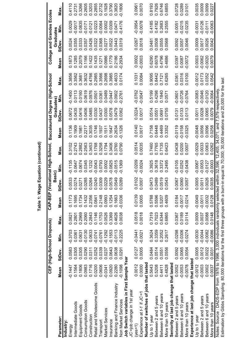
Para

met

er:

Mea

nSt

Dev

.M

in.

Max

.M

ean

StD

ev.

Min

.M

ax.

Mea

nSt

Dev

.M

in.

Max

.M

ean

StD

ev.

Min

.M

ax.

Indu

stry

:

E

nerg

y

-0.1

447

0.05

83-0

.370

30.

0821

0.11

730.

0533

-0.1

135

0.31

020.

1136

0.06

72-0

.145

00.

3856

0.18

730.

0524

0.00

290.

4110

Inte

rmed

iate

Goo

ds

0.15

640.

0305

0.03

610.

2801

0.16

950.

0274

0.06

470.

2743

0.19

090.

0435

0.01

130.

3562

0.12

850.

0355

-0.0

017

0.27

31E

quip

men

t Goo

ds

0.18

060.

0305

0.06

310.

2969

0.17

340.

0271

0.06

740.

2882

0.19

810.

0416

0.01

600.

3681

0.20

790.

0333

0.08

350.

3266

Con

sum

ptio

n G

oods

0.

0983

0.02

90-0

.013

00.

2060

0.14

320.

0285

0.03

450.

2563

0.22

170.

0406

0.06

190.

3632

0.11

660.

0357

-0.0

171

0.26

05C

onst

ruct

ion

0.17

160.

0311

0.06

330.

2843

0.23

560.

0264

0.12

320.

3453

0.30

350.

0485

0.09

760.

4766

0.14

220.

0426

-0.0

121

0.32

03R

etai

l and

Who

leso

me

Goo

ds

0.02

000.

0252

-0.0

741

0.11

460.

0841

0.02

40-0

.004

30.

1768

0.17

460.

0330

0.05

010.

2985

0.14

350.

0322

0.02

230.

2855

Tran

spor

t 0.

0606

0.03

39-0

.076

10.

1753

0.21

480.

0309

0.07

930.

3258

0.19

370.

0437

0.03

610.

3566

0.12

710.

0368

-0.0

064

0.27

32M

arke

t Ser

vice

s -0

.034

10.

0237

-0.1

292

0.05

260.

0993

0.02

290.

0002

0.17

940.

1511

0.03

000.

0489

0.26

980.

0986

0.02

770.

0002

0.19

28In

sura

nce

0.09

200.

0643

-0.1

553

0.33

690.

1254

0.05

78-0

.082

50.

3406

0.16

470.

0578

-0.0

447

0.39

850.

1779

0.05

22-0

.030

90.

3790

Ban

king

and

Fin

ance

Indu

stry

0.

2280

0.06

38-0

.011

30.

4626

0.16

630.

0549

-0.0

515

0.37

600.

2634

0.04

790.

0902

0.46

330.

2186

0.04

430.

0471

0.38

20N

on M

arke

t Ser

vice

s -0

.109

80.

0291

-0.2

225

0.00

38-0

.033

60.

0289

-0.1

369

0.07

90-0

.132

60.

0362

-0.2

761

0.01

74-0

.293

40.

0319

-0.4

176

-0.1

806

Job

Switc

h va

riabl

es in

Firs

t Sam

ple

Year

JC=j

ob c

hang

e in

1st

yea

r (y

es=1

) 0.

0012

0.01

27-0

.044

10.

0518

0.01

390.

0102

-0.0

209

0.05

140.

0140

0.02

24-0

.076

20.

1031

0.00

020.

0267

-0.0

954

0.09

61E

xper

ienc

e at

t-1

if J

C=1

0.

0000

0.00

05-0

.002

10.

0018

0.00

050.

0007

-0.0

024

0.00

350.

0017

0.00

17-0

.004

70.

0084

-0.0

003

0.00

18-0

.007

80.

0070

Num

ber o

f sw

itche

s of

jobs

that

last

edU

p to

1 y

ear

0.

5643

0.04

840.

3624

0.73

190.

5788

0.04

730.

3925

0.74

600.

7158

0.05

140.

5199

0.90

950.

6290

0.04

810.

4185

0.81

93B

etw

een

2 an

d 5

year

s

0.52

080.

0514

0.33

590.

7023

0.55

960.

0489

0.36

180.

7765

0.64

480.

0551

0.42

980.

8442

0.60

780.

0508

0.41

820.

7926

Bet

wee

n 6

and

10 y

ears

0.44

110.

0551

0.20

520.

6344

0.52

070.

0519

0.33

720.

7135

0.44

690.

0691

0.18

400.

7121

0.47

960.

0555

0.26

830.

6746

Mor

e th

an 1

0 ye

ars

0.

4828

0.05

560.

2617

0.68

650.

4609

0.05

430.

2495

0.64

230.

3352

0.07

550.

0571

0.62

650.

4686

0.05

680.

2555

0.68

55Se

nior

ity a

t las

t job

cha

nge

that

last

edB

etw

een

2 an

d 5

year

s 0.

0052

0.00

92-0

.029

80.

0367

0.01

840.

0067

-0.0

105

0.04

38-0

.011

90.

0131

-0.0

601

0.03

610.

0397

0.00

920.

0051

0.07

28B

etw

een

6 an

d 10

yea

rs

-0.0

053

0.00

65-0

.030

60.

0189

-0.0

017

0.00

60-0

.025

20.

0200

-0.0

158

0.01

33-0

.072

60.

0316

0.00

870.

0057

-0.0

215

0.02

89M

ore

than

10

year

s

-0.0

078

0.00

54-0

.027

40.

0114

-0.0

214

0.00

57-0

.043

80.

0007

-0.0

325

0.01

13-0

.076

40.

0100

-0.0

072

0.00

46-0

.023

50.

0101

Expe

rienc

e at

last

job

chan

ge th

at la

sted

Up

to 1

yea

r -0

.001

20.

0005

-0.0

030

0.00

09-0

.004

90.

0005

-0.0

067

-0.0

029

-0.0

048

0.00

11-0

.008

3-0

.001

20.

0003

0.00

09-0

.003

10.

0035

Bet

wee

n 2

and

5 ye

ars

-0

.000

30.

0012

-0.0

044

0.00

37-0

.001

10.

0011

-0.0

053

0.00

330.

0056

0.00

28-0

.004

60.

0173

-0.0

062

0.00

17-0

.012

60.

0009

Bet

wee

n 6

and

10 y

ears

0.

0002

0.00

22-0

.008

20.

0088

-0.0

032

0.00

26-0

.012

70.

0063

0.00

960.

0065

-0.0

120

0.03

52-0

.002

00.

0026

-0.0

111

0.00

99M

ore

than

10

year

s

0.00

370.

0031

-0.0

086

0.01

480.

0128

0.00

35-0

.000

30.

0262

0.02

580.

0079

-0.0

064

0.05

420.

0079

0.00

42-0

.006

30.

0227

CAP

-BEP

(Voc

atio

nal H

igh-

Scho

ol,

Bas

ic)

Not

es: S

ourc

e : D

AD

S-E

DP

from

197

6 to

199

6. 3

,000

indi

vidu

als

rand

omly

sel

ecte

d w

ithin

32,

596;

12,

405;

34,

071;

and

7,5

79 re

spec

tivel

y.

Est

imat

ion

by G

ibbs

Sam

plin

g. 8

0,00

0 ite

ratio

ns fo

r the

firs

t thr

ee g

roup

s w

ith a

bur

n-in

equ

al to

70,

000;

30,

000

itera

tions

and

20,

000

for t

he la

st

Tabl

e 1:

Wag

e Eq

uatio

n (c

ontin

ued)

CEP

(Hig

h-Sc

hool

Dro

pout

s)B

acca

laur

éat D

egre

e (H

igh-

Scho

ol

Gra

duat

es)

Col

lege

and

Gra

ndes

Eco

les

Gra

duat

es

Para

met

er:

Mea

nSt

Dev

.M

in.

Max

.M

ean

StD

ev.

Min

.M

ax.

Mea

nSt

Dev

.M

in.

Max

.M

ean

StD

ev.

Min

.M

ax.

Inte

rcep

t -1

.137

50.

2254

-2.0

040

-0.2

941

-1.1

732

0.22

74-1

.973

0-0

.269

3-0

.857

50.

2244

-1.6

982

0.04

98-0

.745

60.

2288

-1.7

444

0.14

11Ex

perie

nce

0.17

170.

0050

0.15

340.

1914

0.29

540.

0055

0.27

550.

3147

0.39

860.

0059

0.37

770.

4203

0.14

350.

0053

0.12

480.

1654

Expe

rienc

e sq

uare

d -0

.003

10.

0001

-0.0

035

-0.0

028

-0.0

055

0.00

01-0

.005

8-0

.005

0-0

.007

90.

0001

-0.0

083

-0.0

074

-0.0

033

0.00

01-0

.003

8-0

.002

9Lo

cal U

nem

ploy

men

t Rat

e 7.

2233

0.30

146.

0385

8.16

028.

7965

0.35

357.

5332

10.1

660

6.24

700.

2813

5.04

107.

5074

6.36

820.

5105

4.18

968.

1078

Lagg

ed V

aria

bles

:La

gged

Mob

ility γM

1.

4515

0.01

841.

3928

1.52

741.

1894

0.01

871.

1203

1.25

500.

8826

0.01

770.

8172

0.95

281.

0206

0.02

000.

9467

1.10

10La

gged

Par

ticip

atio

n γY

0.14

560.

0098

0.11

480.

1835

0.11

910.

0098

0.08

030.

1574

0.08

850.

0095

0.05

600.

1207

0.18

800.

0094

0.15

240.

2284

Sex

(equ

al to

1 fo

r men

)0.

1815

0.04

210.

0343

0.30

410.

0921

0.04

08-0

.062

90.

2414

-0.0

919

0.04

11-0

.223

10.

0440

0.30

570.

0471

0.16

880.

4835

Chi

ldre

n be

twee

n 0

and

3-0

.385

00.

0333

-0.5

048

-0.2

624

-0.2

215

0.02

84-0

.334

5-0

.114

0-0

.235

50.

0335

-0.3

653

-0.1

158

0.06

380.

0323

-0.0

653

0.19

25C

hild

ren

betw

een

3 an

d 6

-0.3

068

0.03

11-0

.419

3-0

.186

6-0

.269

60.

0286

-0.3

853

-0.1

625

-0.2

880

0.03

67-0

.413

2-0

.147

3-0

.029

50.

0324

-0.1

673

0.10

63Li

ves

in C

oupl

e

-0.1

690

0.03

98-0

.318

6-0

.007

6-0

.271

70.

0406

-0.4

244

-0.1

234

-0.1

940

0.04

35-0

.347

1-0

.045

20.

0595

0.04

89-0

.130

00.

2304

Mar

ried

-0

.121

90.

0268

-0.2

191

-0.0

227

-0.1

913

0.02

98-0

.288

9-0

.070

5-0

.229

80.

0301

-0.3

426

-0.1

197

0.04

210.

0354

-0.0

936

0.16

48Li

ves

in re

gion

Ile

de F

ranc

e 0.

0929

0.03

61-0

.032

40.

2221

0.10

060.

0377

-0.0

416

0.25

090.

0566

0.02

57-0

.038

20.

1457

5.82

020.

2312

5.07

496.

4415

Nat

iona

lity:

Oth

er th

an F

renc

h -0

.267

60.

0471

-0.4

200

-0.1

047

-0.3

383

0.05

18-0

.521

9-0

.143

2-0

.212

40.

0479

-0.3

719

-0.0

462

-0.2

358

0.04

41-0

.383

7-0

.078

8Fa

ther

oth

er th

an F

renc

h -0

.017

40.

1726

-0.5

539

0.63

46-0

.203

30.

1028

-0.5

343

0.15

11-0

.086

50.

0973

-0.4

581

0.22

26-0

.017

10.

1254

-0.3

995

0.41

22M

othe

r oth

er th

an F

renc

h -0

.090

70.

1483

-0.6

944

0.39

560.

0759

0.11

44-0

.314

30.

5599

-0.0

574

0.08

88-0

.375

00.

2653

0.08

510.

1125

-0.2

942

0.47

20C

ohor

t Effe

cts:

Bo

rn b

efor

e 19

29

-2.7

065

0.05

98-2

.909

3-2

.488

6-3

.595

60.

1139

-3.9

867

-3.1

516

-3.4

916

0.11

93-3

.933

8-3

.082

7-2

.576

60.

0943

-2.9

706

-2.2

175

Born

bet

wee

n 19

30 a

nd 1

939

-2.3

839

0.07

10-2

.650

6-2

.137

2-3

.487

60.

0876

-3.9

045

-3.2

078

-4.4

233

0.11

19-4

.895

7-4

.032

7-2

.442

10.

0865

-2.7

478

-2.0

839

Born

bet

wee

n 19

40 a

nd 1

949

-1.9

668

0.07

10-2

.263

2-1

.718

2-3

.069

10.

0743

-3.3

482

-2.7

519

-3.8

498

0.08

99-4

.146

0-3

.543

0-2

.283

60.

0717

-2.5

334

-1.9

232

Born

bet

wee

n 19

50 a

nd 1

959

-1.3

753

0.06

37-1

.633

9-1

.150

1-2

.051

50.

0579

-2.2

560

-1.8

423

-2.0

363

0.05

60-2

.278

4-1

.797

6-2

.012

00.

0613

-2.2

404

-1.7

859

Born

bet

wee

n 19

60 a

nd 1

969

-0.6

219

0.09

11-0

.914

0-0

.275

0-0

.811

70.

0498

-1.0

466

-0.6

440

-0.9

218

0.03

85-1

.064

3-0

.777

9-1

.549

80.

0719

-1.8

007

-1.2

745

Not

es: S

ourc

e : D

ADS-

EDP

from

197

6 to

199

6. 3

,000

indi

vidu

als

rand

omly

sel

ecte

d w

ithin

32,

596;

12,

405;

34,

071;

and

7,5

79 re

spec

tivel

y.

Estim

atio

n by

Gib

bs S

ampl

ing.

80,

000

itera

tions

for t

he fi

rst t

hree

gro

ups

with

a b

urn-

in e

qual

to 7

0,00

0; 3

0,00

0 ite

ratio

ns a

nd 2

0,00

0 fo

r the

last

Tabl

e 2:

Par

ticip

atio

n Eq

uatio

n

CEP

(Hig

h-Sc

hool

Dro

pout

s)B

acca

laur

éat D

egre

e (H

igh-

Scho

ol

Gra

duat

es)

Col

lege

and

Gra

ndes

Eco

les

Gra

duat

esC

AP-B

EP (V

ocat

iona

l Hig

h-Sc

hool

, B

asic

)

Indi

vidu

al a

nd F

amily

Cha

ract

eris

tics:

Para

met

er:

Mea

nSt

Dev

.M

in.

Max

.M

ean

StD

ev.

Min

.M

ax.

Mea

nSt

Dev

.M

in.

Max

.M

ean

StD

ev.

Min

.M

ax.

Inte

rcep

t 2.

0768

0.66

92-0

.052

74.

6419

3.04

250.

9704

0.63

216.

2749

3.18

230.

6672

1.27

655.

0414

0.90

000.

4274

-0.7

862

2.50

78Ex

perie

nce

0.53

960.

1034

0.20

810.

8046

0.56

900.

0957

0.34

340.

8461

0.45

900.

0960

0.14

620.

6643

0.01

050.

0087

-0.0

255

0.04

16Ex

perie

nce

squa

red

-0.0

105

0.00

20-0

.016

2-0

.005

0-0

.008

70.

0026

-0.0

155

-0.0

022

-0.0

058

0.00

29-0

.012

80.

0019

-0.0

004

0.00

02-0

.001

20.

0003

Seni

ority

0.

2730

0.14

010.

0010

0.54

24-0

.220

10.

1309

-0.4

515

0.09

58-0

.076

90.

0808

-0.2

953

0.08

280.

0121

0.00

88-0

.017

20.

0486

Seni

ority

squ

ared

-0.0

076

0.00

54-0

.018

70.

0036

0.00

490.

0067

-0.0

106

0.01

770.

0024

0.00

41-0

.007

70.

0118

-0.0

006

0.00

04-0

.001

90.

0006

Loca

l Une

mpl

oym

ent R

ate

0.22

151.

0307

-3.4

492

3.72

780.

1010

0.98

14-3

.484

23.

8917

0.30

520.

9760

-3.5

975

3.87

240.

6457

0.69

62-2

.165

13.

2531

Part

Tim

e 0.

3200

0.48

90-0

.967

01.

3546

0.55

390.

3695

-0.4

958

1.65

760.

0314

0.38

61-1

.160

30.

9916

-0.4

730

0.04

10-0

.609

0-0

.315

4La

gged

Var

iabl

es:

Lagg

ed M

obilit

y γ

1.04

200.

3071

0.47

911.

7680

0.24

360.

2115

-0.2

504

0.70

45-0

.455

50.

2362

-0.9

903

0.26

760.

0276

0.04

15-0

.105

50.

1717

Indi

vidu

al a

nd F

amily

Cha

ract

eris

tics:

Sex

1.30

450.

6700

-0.2

051

2.58

130.

4414

0.63

60-0

.944

81.

7622

0.30

180.

4045

-0.8

375

1.49

62-0

.139

70.

0613

-0.3

470

0.10

09C

hild

ren

betw

een

0 an

d 3

0.49

760.

6191

-0.9

096

2.47

60-0

.153

90.

5621

-1.6

982

0.97

340.

3433

0.83

18-1

.460

82.

3896

0.05

230.

0479

-0.1

435

0.24

43C

hild

ren

betw

een

3 an

d 6

-0.3

931

0.62

55-2

.182

01.

1188

-0.3

149

0.50

39-1

.336

90.

9304

0.06

061.

0302

-1.8

376

2.75

930.

0611

0.04

72-0

.102

50.

2307

Mar

ried

-0

.625

30.

6188

-1.9

813

0.62

230.

0300

0.34

54-0

.854

40.

9412

0.55

660.

9155

-0.9

050

2.76

150.

1996

0.05

59-0

.006

60.

4296

Live

s in

Cou

ple

0.44

950.

9565

-1.8

453

2.08

571.

0584

0.68

27-0

.503

92.

6736

-0.0

651

0.74

81-1

.841

41.

7181

0.10

600.

0800

-0.1

951

0.38

84Li

ves

in re

gion

Ile

de F

ranc

e -0

.092

60.

6084

-1.3

876

1.33

030.

8778

1.00

81-1

.379

12.

6800

0.81

530.

4044

-0.1

589

1.89

33-0

.197

10.

0520

-0.4

330

-0.0

044

Nat

iona

lity

Oth

er th

an F

renc

h -0

.049

60.

6347

-1.3

465

2.03

11-0

.056

80.

7453

-1.7

824

1.35

260.

0634

0.64

24-1

.129

71.

9631

0.03

320.

0592

-0.1

551

0.25

08Fa

ther

oth

er th

an F

renc

h 0.

5663

0.77

52-1

.557

02.

6507

0.34

530.

7850

-1.8

083

2.47

72-0

.120

40.

5706

-1.5

624

1.35

030.

1121

0.15

67-0

.577

30.

7734

Mot

her o

ther

than

Fre

nch

0.47

390.

7163

-1.9

174

2.77

250.

0517

1.05

13-2

.799

03.

0469

0.03

150.

7974

-1.5

461

1.92

93-0

.249

40.

1359

-0.7

371

0.25

86C

ohor

t Effe

cts

Born

bef

ore

1929

0.

1461

0.73

16-2

.636

32.

8522

-0.1

275

0.88

61-3

.620

52.

5929

0.28

121.

0451

-3.0

258

3.53

261.

1003

0.39

11-0

.440

02.

8883

Born

bet

wee

n 19

30 a

nd 1

939

-1.4

814

0.55

22-3

.290

30.

5178

0.12

450.

8311

-2.6

538

2.11

18-0

.335

50.

9749

-2.8

263

2.40

970.

7095

0.36

52-0

.796

92.

4092

Born

bet

wee

n 19

40 a

nd 1

949

0.58

220.

6294

-1.2

925

2.34

500.

7670

0.61

69-1

.135

02.

5540

-0.0

346

0.85

42-2

.187

62.

7618

0.38

940.

3526

-0.8

703

1.93

06Bo

rn b

etw

een

1950

and

195

9 0.

8313

0.48

38-0

.706

32.

5172

0.26

430.

7417

-1.3

779

2.62

240.

3555

0.56

37-1

.158

92.

2134

-0.0

105

0.34

92-1

.243

41.

4603

Born

bet

wee

n 19

60 a

nd 1

969

1.26

150.

6308

-0.9

655

3.18

501.

0159

0.65

11-0

.620

43.

0558

0.44

000.

6685

-1.3

531

1.87

18-0

.326

50.

3501

-1.5

816

1.01

14In

dust

ryEn

ergy

0.

1766

1.09

65-2

.106

03.

1748

0.04

720.

9691

-2.7

353

2.61

650.

1984

0.87

04-2

.494

22.

1947

0.85

890.

1870

0.18

171.

5324

Inte

rmed

iate

Goo

ds

0.10

450.

7145

-2.0

907

2.40

420.

7122

0.77

96-0

.672

03.

6010

-0.3

831

0.55

66-1

.894

61.

2588

0.33

330.

1342

-0.1

212

0.81

48Eq

uipm

ent G

oods

0.

8554

0.51

05-0

.846

02.

1046

-0.5

386

0.61

05-1

.845

01.

5520

-0.1

609

0.53

49-1

.659

31.

5860

0.44

010.

1294

0.01

640.

8694

Con

sum

ptio

n G

oods

0.

4125

0.66

89-0

.993

72.

0925

0.03

980.

5209

-1.4

037

1.62

980.

3966

0.89

95-1

.824

92.

8584

0.39

200.

1356

-0.1

227

0.94

27C

onst

ruct

ion

-0.0

796

0.73

32-1

.897

71.

6596

1.09

260.

7752

-1.1

446

2.96

280.

1534

0.82

76-2

.265

42.

0930

0.06

720.

1514

-0.4

570

0.58

19R

etai

l and

Who

leso

me

Goo

ds

0.22

200.

6971

-1.7

581

2.13

620.

6457

0.82

89-1

.287

52.

6942

0.59

520.

8010

-1.2

190

2.47

800.

3799

0.13

08-0

.119

40.

8332

Tran

spor

t 0.

4409

0.75

12-1

.791

33.

1346

-0.0

717

0.74

46-1

.805

01.

9270

0.61

890.

7810

-1.5

800

2.51

940.

6788

0.14

560.

1993

1.29

70M

arke

t Ser

vice

s -0

.038

50.

5675

-1.4

497

1.62

680.

4735

0.64

78-1

.204

92.

1805

0.37

040.

4935

-1.0

127

1.94

750.

3927

0.12

06-0

.045

80.

8320

Insu

ranc

e 0.

0604

0.78

87-3

.020

42.

3840

0.01

651.

0426

-2.8

717

2.83

640.

1961

0.71

15-2

.078

92.

2508

0.57

490.

1875

-0.0

964

1.32

16Ba

nkin

g an

d Fi

nanc

e In

dust

ry

-0.3

500

1.08

47-3

.468

93.

8777

0.41

770.

9146

-1.9

790

2.58

660.

9974

0.60

82-0

.445

82.

8591

0.66

380.

1546

0.13

941.

1732

Non

Mar

ket S

ervi

ces

0.23

750.

6835

-1.4

936

1.94

930.

3045

0.98

20-1

.850

42.

9131

0.27

350.

5716

-1.1

924

1.79

830.

4756

0.13

08-0

.010

10.

9290

Not

es: S

ourc

e : D

ADS-

EDP

from

197

6 to

199

6. 3

,000

indi

vidu

als

rand

omly

sel

ecte

d w

ithin

32,

596;

12,

405;

34,

071;

and

7,5

79 re

spec

tivel

y.

Estim

atio

n by

Gib

bs S

ampl

ing.

80,

000

itera

tions

for t

he fi

rst t

hree

gro

ups

with

a b

urn-

in e

qual

to 7

0,00

0; 3

0,00

0 ite

ratio

ns a

nd 2

0,00

0 fo

r the

last

CAP

-BEP

(Voc

atio

nal H

igh-

Scho

ol,

Bas

ic)

Tabl

e 3:

Mob

ility

Equ

atio

n

CEP

(Hig

h-Sc

hool

Dro

pout

s)B

acca

laur

éat D

egre

e (H

igh-

Scho

ol

Gra

duat

es)

Col

lege

and

Gra

ndes

Eco

les

Gra

duat

es

Initi

al P

artic

ipat

ion

Mea

nSt

Dev

.M

in.

Max

.M

ean

StD

ev.

Min

.M

ax.

Mea

nSt

Dev

.M

in.

Max

.M

ean

StD

ev.

Min

.M

ax.

Inte

rcep

t -1

.104

90.

3721

-2.4

940

0.44

08-1

.304

50.

3763

-2.8

871

0.14

30-2

.143

80.

3995

-3.6

831

-0.4

294

-1.9

636

0.42

65-3

.638

2-0

.448

5Ex

perie

nce

0.00

400.

0221

-0.0

834

0.07

690.

1445

0.02

250.

0552

0.23

990.

1200

0.02

590.

0203

0.23

890.

0389

0.01

61-0

.028

70.

1033

Expe

rienc

e sq

uare

d 0.

0008

0.00

04-0

.000

80.

0026

-0.0

032

0.00

06-0

.006

2-0

.000

8-0

.001

80.

0007

-0.0

044

0.00

06-0

.000

50.

0005

-0.0

025

0.00

14Lo

cal U

nem

ploy

men

t Rat

e 1.

4790

0.95

00-2

.232

64.

9118

1.25

460.

9325

-2.3

890

4.57

631.

5701

0.93

67-1

.703

64.

8433

-0.1

528

0.97

71-3

.940

83.

4815

Sex

(equ

al to

1 fo

r men

)

0.41

850.

0709

0.16

290.

6876

0.54

030.

0802

0.23

580.

8083

0.35

560.

1011

-0.0

670

0.74

270.

5894

0.09

630.

2243

0.94

77C

hild

ren

betw

een

0 an

d 3

-0.3

160

0.10

19-0

.668

00.

1912

-0.4

859

0.10

99-0

.896

5-0

.037

5-0

.015

70.

1578

-0.5

814

0.58

54-0

.143

20.

1294

-0.6

354

0.33

60C

hild

ren

betw

een

3 an

d 6

-0.2

801

0.10

60-0

.674

20.

1319

-0.4

825

0.12

11-0

.892

20.

0579

0.06

170.

1825

-0.8

113

0.80

10-0

.038

10.

1286

-0.5

044

0.39

12M

arrie

d

0.20

480.

0844

-0.1

450

0.52

880.

4972

0.10

480.

1626

0.87

060.

2742

0.12

88-0

.306

50.

8207

0.64

590.

1087

0.25

141.

0670

Live

s in

regi

on Il

e de

Fra

nce

0.05

350.

1132

-0.4

016

0.48

99-0

.041

20.

1299

-0.5

100

0.47

010.

1329

0.15

01-0

.431

90.

7393

4.71

860.

4037

3.63

996.

2068

Oth

er th

an F

renc

h -0

.070

30.

0836

-0.4

245

0.28

68-0

.177

10.

0904

-0.5

200

0.15

340.

1094

0.10

06-0

.240

50.

5141

0.23

650.

0819

-0.0

870

0.52

01Fa

ther

oth

er th

an F

renc

h -0

.591

50.

3110

-1.7

487

0.38

380.

0976

0.19

83-0

.677

40.

8976

-0.2

553

0.37

13-1

.956

30.

8891

0.02

280.

3773

-1.6

193

1.34

43M

othe

r oth

er th

an F

renc

h -0

.498

30.

3628

-1.9

284

0.63

61-0

.319

40.

2603

-1.5

939

0.55

97-0

.469

00.

4222

-2.3

750

1.02

02-0

.744

90.

3854

-2.0

413

0.55

17In

itial

Mob

ility

Inte

rcep

t 1.

9944

0.75

32-1

.220

64.

3769

2.19

040.

7448

-1.0

036

5.29

221.

5920

0.79

82-1

.191

44.

8785

0.96

660.

5525

-1.0

883

2.84

13Ex

perie

nce

0.45

270.

1945

-0.1

077

1.01

160.

6157

0.22

43-0

.048

71.

1835

0.72

780.

2355

-0.0

083

1.30

220.

0010

0.02

93-0

.118

00.

1438

Expe

rienc

e sq

uare

d -0

.006

40.

0050

-0.0

188

0.00

800.

0005

0.00

62-0

.015

10.

0207

-0.0

127

0.00

70-0

.029

20.

0081

0.00

000.

0009

-0.0

039

0.00

36Se

nior

ity

-0.1

997

0.30

00-0

.941

20.

5127

0.21

210.

3626

-0.7

626

1.30

410.

4300

0.54

27-1

.197

31.

6984

-0.0

802

0.04

04-0

.231

20.

0599

Seni

ority

squ

ared

0.00

880.

0186

-0.0

351

0.05

770.

0215

0.02

48-0

.031

70.

0831

0.00

160.

0311

-0.0

553

0.10

530.

0031

0.00

23-0

.005

00.

0114

Loca

l Une

mpl

oym

ent R

ate

0.10

370.

9985

-3.8

532

3.79

830.

1182

0.98

91-4

.023

73.

9986

0.09

491.

0023

-4.1

586

3.99

860.

0834

0.99

94-3

.598

74.

0413

Sex

(equ

al to

1 fo

r men

)

0.66

160.

7829

-1.3

483

2.61

870.

9083

0.67

83-1

.474

72.

9115

0.47

840.

7386

-2.0

752

2.57

79-0

.145

30.

1776

-0.7

775

0.60

63C

hild

ren

betw

een

0 an

d 3

0.31

250.

7709

-1.9

758

2.56

670.

0804

0.94

80-2

.295

53.

4939

0.38

130.

9485

-2.3

097

3.20

160.

1331

0.19

74-0

.655

30.

9201

Chi

ldre

n be

twee

n 3

and

60.

1879

0.98

66-3

.078

72.

8965

0.01

730.

8554

-2.3

229

2.84

90-0

.203

50.

9725

-3.3

708

2.81

450.

0608

0.20

55-0

.698

30.

8129

Mar

ried

0.

0028

0.66

43-2

.026

32.

2416

0.20

600.

8908

-1.9

908

2.75

650.

0279

0.85

04-2

.502

83.

2804

0.39

960.

1784

-0.2

644

1.03

38Li

ves

in re

gion

Ile

de F

ranc

e-0

.052

80.

9751

-2.6

563

4.12

170.

1092

1.05

27-2

.601

03.

3143

0.18

130.

8262

-2.2

608

3.02

43-0

.311

00.

1447

-0.8

127

0.25

60O

ther

than

Fre

nch

0.34

400.

7863

-2.3

366

2.25

870.

0603

0.79

14-2

.332

82.

3200

0.37

000.

7290

-1.4

243

3.72

120.

2506

0.14

69-0

.304

20.

8513

Fath

er o

ther

than

Fre

nch

0.09

100.

9335

-3.7

647

3.40

350.

1031

0.90

50-2

.529

43.

2658

0.02

790.

9765

-3.8

312

3.42

37-0

.446

90.

5608

-2.4

698

1.46

72M

othe

r oth

er th

an F

renc

h 0.

0939

0.95

84-3

.002

73.

8895

0.08

010.

9286

-3.0

826

3.06

460.

0157

0.98

80-3

.523

13.

6970

0.13

150.

6210

-2.0

247

2.51

81N

otes

: Sou

rce

: DAD

S-ED

P fro

m 1

976

to 1

996.

3,0

00 in

divi

dual

s ra

ndom

ly s

elec

ted

with

in 3

2,59

6; 1

2,40

5; 3

4,07

1; a

nd 7

,579

resp

ectiv

ely.

Es

timat

ion

by G

ibbs

Sam

plin

g. 8

0,00

0 ite

ratio

ns fo

r the

firs

t thr

ee g

roup

s w

ith a

bur

n-in

equ

al to

70,

000;

30,

000

itera

tions

and

20,

000

for t

he la

st

Tabl

e 4:

Initi

al P

artic

ipat

ion

and

Initi

al M

obili

ty E

quat

ions

CEP

(Hig

h-Sc

hool

Dro

pout

s)B

acca

laur

éat D

egre

e (H

igh-

Scho

ol

Gra

duat

es)

Col

lege

and

Gra

ndes

Eco

les

Gra

duat

esC

AP-B

EP (V

ocat

iona

l Hig

h-Sc

hool

, B

asic

)

Indi

vidu

al E

ffect

s:M

ean

StD

ev.

Min

.M

ax.

Mea

nSt

Dev

.M

in.

Max

.M

ean

StD

ev.

Min

.M

ax.

Mea

nSt

Dev

.M

in.

Max

.ρ y

0m0

0.

0105

0.02

00-0

.032

30.

0600

0.00

190.

0245

-0.0

464

0.06

360.

0188

0.02

56-0

.039

40.

0844

-0.0

076

0.02

58-0

.059

60.

0550

ρ y0y

0.21

360.

0250

0.13

190.

2537

0.03

220.

0190

-0.0

130

0.09

080.

0426

0.03

08-0

.021

10.

1018

0.10

680.

0147

0.06

110.

1372

ρ y0w

0.19

810.

0169

0.16

160.

2370

-0.0

069

0.01

97-0

.054

40.

0323

0.03

600.

0249

-0.0

086

0.09

310.

0521

0.01

950.

0073

0.09

19ρ y

0m

-0

.045

50.

0270

-0.1

002

0.00

53-0

.012

50.

0202

-0.0

598

0.03

620.

0147

0.01

90-0

.035

20.

0694

-0.0

016

0.03

18-0

.076

80.

0556

ρ m0y

0.01

210.

0321

-0.0

492

0.08

24-0

.022

30.

0263

-0.0

622

0.04

000.

0067

0.02

09-0

.048

80.

0438

0.02

810.

0255

-0.0

437

0.08

86ρ m

0w

0.

0070

0.03

09-0

.073

50.

0720

-0.0

296

0.02

08-0

.078

20.

0154

0.02

350.

0179

-0.0

162

0.06

65-0

.011

10.

0193

-0.0

524

0.02

63ρ m

0m

-0

.017

30.

0205

-0.0

685

0.03

140.

0298

0.02

36-0

.018

90.

0810

-0.0

271

0.02

04-0

.069

20.

0238

-0.0

006

0.05

61-0

.073

90.

1096

ρ yw

0.36

270.

0331

0.29

240.

4328

0.40

200.

0380

0.34

710.

4995

0.31

930.

0291

0.26

030.

3812

0.14

540.

0426

0.06

300.

2345

ρ ym

-0.0

204

0.02

44-0

.075

00.

0325

-0.0

225

0.02

50-0

.077

50.

0404

-0.0

260

0.01

89-0

.065

60.

0206

-0.0

322

0.04

01-0

.118

50.

0419

ρ wm

-0.0

435

0.03

48-0

.099

30.

0285

-0.0

415

0.04

04-0

.114

60.

0239

-0.0

819

0.02

39-0

.140

9-0

.030

9-0

.010

00.

0246

-0.0

855

0.03

82Id

iosy

ncra

tic E

ffect

s:

σ20.

2846

0.00

150.

2786

0.29

440.

2722

0.00

170.

2650

0.28

070.

6563

0.00

650.

6365

0.68

090.

4026

0.00

340.

3934

0.41

50ρ w

m

0.

1296

0.12

40-0

.157

50.

4311

-0.0

151

0.13

06-0

.338

50.

3077

0.02

960.

0631

-0.1

867

0.20

460.

1160

0.01

350.

0000

0.17

18ρ y

m

0.

1277

0.26

99-0

.420

30.

6082

0.15

870.

2627

-0.3

142

0.69

290.

4225

0.24

26-0

.369

00.

7210

-0.0

506

0.04

92-0

.255

10.

1005

ρ yw

0.05

520.

0159

-0.0

086

0.11

36-0

.040

30.

0145

-0.1

048

0.02

090.

0989

0.03

20-0

.018

70.

1970

-0.0

170

0.02

11-0

.097

50.

0635

Not

es: S

ourc

e : D

AD

S-E

DP

from

197

6 to

199

6. 3

,000

indi

vidu

als

rand

omly

sel

ecte

d w

ithin

32,

596;

12,

405;

34,

071;

and

7,5

79

resp

ectiv

ely.

Est

imat

ion

by G

ibbs

Sam

plin

g. 8

0,00

0 ite

ratio

ns fo

r the

firs

t thr

ee g

roup

s w

ith a

bur

n-in

equ

al to

70,

000;

30,

000

itera

tions

Tabl

e 5:

Var

ianc

e-C

ovar

ianc

e M

atric

es (I

ndiv

idua

l and

Idio

sync

ratic

Effe

cts)

CEP

(Hig

h-Sc

hool

Dro

pout

s)B

acca

laur

éat D

egre

e (H

igh-

Scho

ol

Gra

duat

es)

Col

lege

and

Gra

ndes

Eco

les

Gra

duat

esC

AP-B

EP (V

ocat

iona

l Hig

h-Sc

hool

, B

asic

)

Parameters: Mean StDev. Min. Max. Mean StDev. Min. Max.Wage Equation: Experience 0.0580 0.0032 0.0518 0.0643 0.0674 0.0031 0.0553 0.0799Experience squared -0.0013 0.0001 -0.0015 -0.0012 -0.0011 0.0001 -0.0013 -0.0008Seniority 0.0518 0.0029 0.0460 0.0576 0.0094 0.0022 0.0001 0.0196Seniority squared -0.0005 0.0001 -0.0007 -0.0004 -0.0002 0.0001 -0.0005 0.0002Number of switches of jobs that lasted:Up to 1 year 0.2240 0.0172 0.1905 0.2572 0.6290 0.0481 0.4185 0.8193Between 2 and 5 years 0.1648 0.0189 0.1274 0.2018 0.6078 0.0508 0.4182 0.7926Between 6 and 10 years 0.3231 0.0683 0.1861 0.4572 0.4796 0.0555 0.2683 0.6746More than 10 years 0.4717 0.0869 0.3031 0.6425 0.4686 0.0568 0.2555 0.6855Seniority at last job change that lasted: Between 2 and 5 years 0.0567 0.0070 0.0432 0.0709 0.0397 0.0092 0.0051 0.0728Between 6 and 10 years 0.0111 0.0097 -0.0079 0.0303 0.0087 0.0057 -0.0215 0.0289More than 10 years 0.0062 0.0055 -0.0050 0.0166 -0.0072 0.0046 -0.0235 0.0101Experience at last job change that lasted:Up to 1 year -0.0071 0.0016 -0.0102 -0.0040 0.0003 0.0009 -0.0031 0.0035Between 2 and 5 years -0.0058 0.0016 -0.0090 -0.0027 -0.0062 0.0017 -0.0126 0.0009Between 6 and 10 years -0.0025 0.0025 -0.0073 0.0024 -0.0020 0.0026 -0.0111 0.0099More than 10 years -0.0026 0.0033 -0.0090 0.0036 0.0079 0.0042 -0.0063 0.0227Participation Equation:Lagged Mobility γM 0.3336 0.1646 0.0111 0.6274 1.0206 0.0200 0.9467 1.1010Lagged Participation γY 2.0046 0.0944 1.8178 2.1978 0.1880 0.0094 0.1524 0.2284Mobility Equation:Seniority -0.0878 0.0074 -0.1024 -0.0734 0.0121 0.0088 -0.0172 0.0486Seniority squared 0.0020 0.0003 0.0015 0.0026 -0.0006 0.0004 -0.0019 0.0006Lagged Mobility γ -0.9019 0.0552 -1.0133 -0.7953 0.0276 0.0415 -0.1055 0.1717Individual Effects:ρy0m0 0.8040 0.0556 0.7024 0.9005 -0.0076 0.0258 -0.0596 0.0550ρy0y 0.5716 0.0286 0.5190 0.6224 0.1068 0.0147 0.0611 0.1372ρy0w 0.1335 0.0757 0.0169 0.2714 0.0521 0.0195 0.0073 0.0919ρy0m -0.6044 0.0773 -0.7595 -0.4892 -0.0016 0.0318 -0.0768 0.0556ρm0y 0.2896 0.0429 0.2268 0.3845 0.0281 0.0255 -0.0437 0.0886ρm0w -0.1450 0.0884 -0.2586 0.0403 -0.0111 0.0193 -0.0524 0.0263ρm0m -0.4234 0.0789 -0.5691 -0.2668 -0.0006 0.0561 -0.0739 0.1096ρyw 0.2174 0.0553 0.1066 0.3017 0.1454 0.0426 0.0630 0.2345ρym -0.5061 0.0656 -0.6172 -0.3874 -0.0322 0.0401 -0.1185 0.0419ρwm -0.5352 0.0590 -0.6371 -0.4131 -0.0100 0.0246 -0.0855 0.0382

σ2 0.2062 0.0023 0.2016 0.2104 0.4026 0.0034 0.3934 0.4150ρwm 0.0013 -0.0111 0.0075 0.0161 0.1160 0.0135 0.0000 0.1718ρym -0.0005 0.0113 -0.0217 0.0188 -0.0506 0.0492 -0.2551 0.1005ρyw -0.0496 0.0124 -0.0672 -0.0205 -0.0170 0.0211 -0.0975 0.0635

Idiosyncratic Effects:

Table 6: Comparison United-States vs France (College Graduates)

College Graduates, United States

College or Grandes Ecoles Graduates, France

Parameters: Mean StDev. Min. Max. Mean StDev. Min. Max.Wage Equation:Experience 0.0283 0.0027 0.0229 0.0334 0.0495 0.0027 0.0380 0.0595Experience squared -0.0007 0.0000 -0.0007 -0.0006 -0.0006 0.0000 -0.0008 -0.0004Seniority 0.0517 0.0034 0.0455 0.0580 0.0031 0.0018 -0.0046 0.0097Seniority squared -0.0005 0.0001 -0.0008 -0.0003 -0.0002 0.0001 -0.0005 0.0001Number of switches of jobs that lasted:Up to 1 year 0.0923 0.0144 0.0635 0.1203 0.5643 0.0484 0.3624 0.7319Between 2 and 5 years 0.0958 0.0219 0.0526 0.1386 0.5208 0.0514 0.3359 0.7023Between 6 and 10 years 0.1229 0.1027 -0.0569 0.3076 0.4411 0.0551 0.2052 0.6344More than 10 years 0.2457 0.1078 0.0474 0.4606 0.4828 0.0556 0.2617 0.6865Seniority at last job change that lasted: Between 2 and 5 years 0.0293 0.0084 0.0127 0.0456 0.0052 0.0092 -0.0298 0.0367Between 6 and 10 years 0.0213 0.0109 0.0003 0.0422 -0.0053 0.0065 -0.0306 0.0189More than 10 years 0.0350 0.0053 0.0238 0.0444 -0.0078 0.0054 -0.0274 0.0114Experience at last job change that lasted:Up to 1 year 0.0009 0.0012 -0.0015 0.0033 -0.0012 0.0005 -0.0030 0.0009Between 2 and 5 years -0.0007 0.0016 -0.0038 0.0024 -0.0003 0.0012 -0.0044 0.0037Between 6 and 10 years 0.0007 0.0030 -0.0049 0.0060 0.0002 0.0022 -0.0082 0.0088More than 10 years -0.0090 0.0029 -0.0150 -0.0035 0.0037 0.0031 -0.0086 0.0148Participation Equation:Lagged Mobility γM 0.5295 0.1258 0.3043 0.7836 1.4515 0.0184 1.3928 1.5274Lagged Participation γY 1.7349 0.0660 1.5999 1.8530 0.1456 0.0098 0.1148 0.1835Mobility Equation:Seniority -0.0812 0.0115 -0.1007 -0.0605 0.2730 0.1401 0.0010 0.5424Seniority squared 0.0018 0.0003 0.0011 0.0024 -0.0076 0.0054 -0.0187 0.0036Lagged Mobility γ -0.7190 0.0738 -0.8544 -0.5807 1.0420 0.3071 0.4791 1.7680Individual Effects:ρy0m0 -0.1020 0.1146 -0.2589 0.1067 0.0105 0.0200 -0.0323 0.0600ρy0y 0.7548 0.0566 0.6525 0.8747 0.2136 0.0250 0.1319 0.2537ρy0w 0.3447 0.0351 0.2732 0.4142 0.1981 0.0169 0.1616 0.2370ρy0m 0.0278 0.2007 -0.2908 0.2281 -0.0455 0.0270 -0.1002 0.0053ρm0y 0.1972 0.0746 0.0260 0.2971 0.0121 0.0321 -0.0492 0.0824ρm0w 0.0646 0.0505 -0.0061 0.1794 0.0070 0.0309 -0.0735 0.0720ρm0m -0.0573 0.1666 -0.2619 0.2194 -0.0173 0.0205 -0.0685 0.0314ρyw 0.2958 0.0282 0.2292 0.3560 0.3627 0.0331 0.2924 0.4328ρym -0.2100 0.1053 -0.3832 -0.0429 -0.0204 0.0244 -0.0750 0.0325ρwm -0.2744 0.0799 -0.4083 -0.1348 -0.0435 0.0348 -0.0993 0.0285Idiosyncratic Effects: σ2 0.2448 0.0064 0.2331 0.2539 0.2846 0.0015 0.2786 0.2944ρwm -0.0055 0.0074 -0.0185 0.0072 0.1296 0.1240 -0.1575 0.4311ρym 0.0029 0.0077 -0.0117 0.0160 0.1277 0.2699 -0.4203 0.6082ρyw -0.0346 0.0072 -0.0497 -0.0183 0.0552 0.0159 -0.0086 0.1136

Table 7: Comparison United-States vs France (High-School Dropouts)

High-School Dropouts United States

CEP Graduates France

Varia

ble

Mea

nSt

Err

orM

ean

St E

rror

Mea

nS

t Err

orM

ean

St E

rror

Par

ticip

atio

n 0.

5045

0.50

000.

5953

0.49

080.

4604

0.49

840.

4700

0.49

91W

age

4.08

740.

8093

4.19

480.

7426

4.15

730.

9801

4.70

061.

1599

Mob

ility

0.83

740.

3690

0.84

110.

3656

0.77

270.

4191

0.71

760.

4502

Tenu

re

7.64

767.

8048

6.09

966.

9759

4.11

656.

1718

6.24

677.

7694

Exp

erie

nce

24.7

733

11.4

711

17.3

792

10.6

656

11.7

819

9.99

4515

.783

79.

6285

Live

s in

Cou

ple

0.06

480.

2461

0.06

070.

2388

0.06

610.

2484

0.05

510.

2281

Mar

ried

0.63

470.

4815

0.56

450.

4958

0.35

400.

4782

0.57

060.

4950

Chi

ldre

n be

twee

n 0

and

3 0.

0863

0.28

090.

1329

0.33

950.

1019

0.30

250.

1225

0.32

79C

hild

ren

betw

een

3 an

d 6

0.08

980.

2859

0.11

520.

3192

0.07

490.

2633

0.10

960.

3125

Num

ber o

f Chi

ldre

n 1.

3196

1.37

711.

0769

1.21

860.

5873

0.98

890.

9830

1.42

18Li

ves

in R

egio

n Ile

de

Fran

ce

0.11

960.

3245

0.08

690.

2817

0.15

310.

3600

0.20

880.

4064

Live

s in

Par

is

0.11

820.

3228

0.08

340.

2765

0.15

320.

3602

0.27

070.

4443

Live

s in

Tow

n 0.

2033

0.40

240.

2270

0.41

890.

2417

0.42

810.

2251

0.41

76R

ural

0.

6785

0.46

700.

6896

0.46

270.

6051

0.48

880.

5043

0.50

00

Tabl

e I.1

a: D

escr

iptiv

e St

atis

tics

Not

es: S

ourc

e : D

AD

S-E

DP

from

197

6 to

199

6. 3

2,59

6; 1

2,40

5; 3

4,07

1; a

nd 7

,579

indi

vidu

als

resp

ectiv

ely.

Gra

ndes

Eco

les,

C

olle

ge G

radu

ates

CEP

(Hig

h-Sc

hool

D

ropo

uts)

Bac

cala

uréa

t (H

igh-

Scho

ol G

radu

ates

)C

AP

(Occ

upat

iona

l de

gree

s)

Varia

ble

Mea

nSt

Err

orM

ean

St E

rror

Mea

nS

t Err

orM

ean

St E

rror

Part

Tim

e 0.

1846

0.38

800.

1521

0.35

910.

2394

0.42

670.

2137

0.41

00lo

cal U

nem

ploy

men

t Rat

e 8.

1940

3.63

548.

4130

3.44

298.

2858

3.58

248.

9162

2.77

71Ag

ricul

ture

0.

0416

0.19

970.

0401

0.19

620.

0209

0.14

290.

0130

0.11

33En

ergy

0.

0096

0.09

770.

0149

0.12

100.

0125

0.11

100.

0219

0.14

63In

term

edia

te G

oods

0.

1014

0.30

180.

0991

0.29

880.

0484

0.21

470.

0634

0.24

36Eq

uipm

ent G

oods

0.

1139

0.31

760.

1260

0.33

190.

0665

0.24

910.

1277

0.33

37C

onsu

mpt

ion

Goo

ds

0.11

280.

3164

0.07

380.

2614

0.05

460.

2272

0.05

550.

2289

Con

stru

ctio

n 0.

0870

0.28

190.

1158

0.32

000.

0375

0.19

010.

0357

0.18

56R

etai

l and

Who

leso

me

Goo

ds

0.16

030.

3669

0.14

290.

3499

0.15

610.

3630

0.09

390.

2917

Tran

spor

t 0.

0615

0.24

020.

0602

0.23

780.

0704

0.25

570.

0531

0.22

42M

arke

t Ser

vice

s 0.

2098

0.40

720.

2256

0.41

800.

3161

0.46

500.

3383

0.47

31In

sura

nce

0.00

820.

0900

0.00

880.

0934

0.01

870.

1356

0.01

560.

1238

Bank

ing

and

Fina

nce

Indu

stry

0.

0157

0.12

410.

0242

0.15

360.

0557

0.22

940.

0452

0.20

77N

on M

arke

t Ser

vice

s 0.

0713

0.25

730.

0631

0.24

320.

1358

0.34

260.

1306

0.33

70Bo

rn b

efor

e 19

29

0.23

800.

4258

0.05

150.

2210

0.04

520.

2078

0.09

560.

2941

Born

bet

wee

n 19

30 a

nd 1

939

0.21

320.

4096

0.11

710.

3215

0.04

800.

2137

0.13

140.

3378

Born

bet

wee

n 19

40 a

nd 1

949

0.22

900.

4202

0.20

320.

4024

0.10

480.

3063

0.28

670.

4522

Born

bet

wee

n 19

50 a

nd 1

959

0.23

290.

4227

0.30

990.

4625

0.21

230.

4089

0.32

660.

4690

Born

bet

wee

n 19

60 a

nd 1

969

0.06

460.

2459

0.27

870.

4483

0.44

760.

4973

0.15

800.

3648

Born

afte

r 197

0

0.02

220.

1475

0.03

980.

1954

0.14

210.

3492

0.00

170.

0417

Tabl

e I.1

b: D

escr

iptiv

e St

atis

tics

(con

tinue

d)

Not

es: S

ourc

e : D

ADS-

EDP

from

197

6 to

199

6. 3

2,59

6; 1

2,40

5; 3

4,07

1; a

nd 7

,579

indi

vidu

als

resp

ectiv

ely.

Gra

ndes

Eco

les,

C

olle

ge G

radu

ates

CEP

(Hig

h-Sc

hool

D

ropo

uts)

Bacc

alau

réat

(Hig

h-Sc

hool

Gra

duat

es)

CAP

(Occ

upat

iona

l de

gree

s)