the rise and fall of technology and the ...org.elon.edu/ipe/gallagher final.pdfissues in political...

Issues in Political Economy, Vol. 12, August 2003

THE RISE AND FALL OF TECHNOLOGY AND THE BUSINESS CYCLE Patrick C. Gallagher, Elon University

In 1997, the first “dot-COM's” began receiving national attention as the media began

talking about the new economy based on the Internet. In 1999, more and more people "entrepreneured" their way into the dot-COM frenzy (Gimein 2001). However, by 2001 the dot-COM boom seemed to be over with estimates of approximately 384 former dot-COM companies collapsing either through bankruptcy or ceased operations in 2001 alone (Florian 2001). As one dot-COM CEO puts it, "'All the tourists came because everybody said it was great, and then when they got there, it was packed, you waited in line for everything, and the food sucked'" (Gimein 2001).

While the technology sector was rising and falling, the US economy followed much of the same trend, so much so that it seemed that the technology sector was driving the economy. Productivity increased nearly one percent per year from 1995 to 1997, and then remained above four percent through 2000. However, in 2001, productivity fell to nearly one percent (Federal Reserve Bank of St. Louis)1. These simultaneous occurrences make one wonder if somehow the two were connected. Paul Krugman's 1994 book, Peddling Prosperity, provides the following hypothesis:

Indeed, since the seminal work of MIT's Robert Solow in the 1950s, analysts of long-run growth have been aware that long-run economic growth would grind to a halt without continuous technological progress, and that such progress is the main source of productivity increase (Krugman 1994, p.59).

Such is the basis of thought lying behind one of the possible explanations of the 1973 productivity slowdown according to Krugman's book. However, this theory would certainly seem just as relevant to the world today as America has just completed an economic "boom" that is unprecedented in history by growing at a rate of more than four percent (Federal Reserve Bank of St. Louis). While the economy has been booming, technology has also been increasing. In addition to the dot-COM's, the latter half of the 1990's has seen the introduction of widespread use of the Internet, cellular phones, and digital personal organizers. According to Krugman (1994), this theory goes on to say that after a while, current technology reaches its limitations, meaning that innovation slows, which leads to a decrease in measures of productivity. Again, after the influx of all of this new technology, America is now in the midst of a recession, and it could be argued that the benefits of this new technology have set in (the "newness" is gone) leading to an economic downturn. Krugman (1994) goes on to say that the productivity slowdown of the early 1970's could be attributed to the same theory because "…the set of technologies that had driven the postwar boom had been pretty much fully exploited, while the technologies that will eventually power another boom were not yet ready for prime time" (Krugman 1994, p.63). So as Krugman (1994) suggests, it is possible that technological innovation could be both a driving force behind long-run growth and fluctuations in the business cycle. This theory is known as the Real Business Cycle theory and has its roots based in the work of Schumpeter (1927) but is based largely on the works of three economists, King, Plosser, and Rebelo (1988a,b)2. This body of literature puts forward the notion of technology controlling both growth and business cycle fluctuations, as opposed to the more classical economic theories


advanced by Keynes (1936) and Friedman and Schwartz (1963), which had a hard time reconciling the dichotomy between growth and fluctuations. These two theories focus on aggregate consumption and the money supply, respectively, as the sources of business cycle fluctuations. The dichotomy between growth and fluctuations exists because although it is usually accepted that technological innovation is the only method for permanent long-run growth, the classical models cannot explain business cycle fluctuations. Similarly, other models can explain fluctuations in the business cycles but cannot explain long-run growth.

The dot-COM's are just one example of technology driving the business cycle. From that example, the purpose of this paper is to look at which theory best explains fluctuations in the US business cycle from 1959-2000. Using the works of Schumpeter (1927) and King, Plosser, and Rebelo (1988a,b) as a starting point, this paper will analyze what Real Business Cycle theory says as compared to more well-known theories of business cycles, such as the Keynesian theory and the Monetarist theory. Then empirical evidence will be shown in an attempt to discover which theory fits the time series data the best. It is the hypothesis of this paper that Real Business Cycle theory will best explain the fluctuations in the business cycle and long-run growth since 1959. An understanding of fluctuations in the business cycle and long-run growth will then give a solid basis for future fiscal policy-making. I. THEORY AND LITERATURE REVIEW A. Neoclassical Growth & Technological Innovation

Joseph Alois Schumpeter's ideas are a forerunner of the Real Business Cycle theory. In his work, "The Explanation of the Business Cycle," Schumpeter (1927) makes the claim that the impulses that are typically thought of as causing the business cycle, such as wars, social unrest, and other exogenous factors affecting the economy, are actually the mechanism of the cycles. His claim is that people's reactions to these disturbances are what develop "Real Business Cycles3" because people can make one of two choices: make slight adjustments to their behavior and adapt to the disturbance or do new things in new ways to face the disturbance. By choosing the latter, people become "innovative," leading to increased productivity. Schumpeter claims that the open-minded and innovative characters of these people "…will always and necessarily find, or be able to create, the opportunity on which to act, being, in fact, itself the one fundamental 'initial impulse' of industrial and commercial change" (Schumpeter 1927, p. 293). He bases this claim on the fact that if a boom in the business cycle were based upon some event outside the realm of economics (Event A), that in the absence of Event A, there would be some other event (Event B) to take its place and have its effect on the business cycle. In other words, there is a plethora of exogenous factors that affect the business cycle, and it is only by chance that they cause an upward or downward movement in the cycle. Schumpeter (1927) then explains the downward trends of the business cycle as an adjustment to the new equilibrium set by the preceding expansion. He further distinguishes this type of recession as a "normal" recession versus an "abnormal" recession which is often brought about by psychological factors such as fear and panic. Schumpeter (1927) explains that innovation is not continuous in time because when an exogenous shock occurs, a small group of people will be daringly innovative. After others realize that what they are doing is profitable, more people join in as well, causing an economic boom. The ensuing recession is just the adjustment of the economy to the newly created equilibrium. One could speculate that is what happened with the recent onslaught and


subsequent failure of the dot-COM's. It seems as though once a few dot-COM's proved successful, everyone jumped on the bandwagon, only to experience market saturation, and now most of them no longer exist (Gimein 2001). One could further assume that due to the saturation and fall-out, the level of innovation has not been constant. In support of this assumption, Thomas Kuhn, a philosopher of science, speculates that innovation is not continuous at all, but rather accelerated by a spurt of innovation followed by a period of a "plateau" (Hutcheon 1995). "The recurring periods of prosperity of the cyclical movement are the form progress takes in capitalistic society" (Schumpeter 1927, p.295). An important aspect of Schumpeter's (1927) theory is that the innovations must work. Krugman (1994) echoes this sentiment by saying that for years personal computers have been in use by many offices, but some say that it is only with a total reorganization of an office integrating that technology that improvements in productivity are realized. So based on both the works of Krugman (1994) and Schumpeter (1927), it is an important note that "workable" technology is what is considered in this theory. As mentioned in Krugman (1994), Robert Solow (1957) finds that increases in technological innovation are the sole cause of long-run growth. Solow (1957) finds that by taking a Cobb-Douglas production function under the assumption of constant returns to scale, the aggregate demand function can be estimated as: (1) Q = A (t) f (K, L) In this equation, Q equals output, A(t) measures technical shifts over time, K is capital, and L is labor. This is now known as the Solow Growth Model. By looking at the forty year period 1909-1949, Solow (1957) finds that aggregate demand shifted upward by about 80 percent, with one-eighth of the increase attributable to increased capital per man hour and seven-eighths attributable to changes in technology. It is important to note that Solow (1957) did find that the average growth rate was around 1 per cent per year for the first half of the period and 2 per cent for the second half. To further support his claim, Solow (1957) notes that other economists who


correlated increased output

Solow's Measures of Technological Innovation (Data: Solow 1957)

0.000

0.200

0.400

0.600

0.800

1.000

1.200

1.400

1.600

1.800

2.000

1909

1911

1913

1915

1917

1919

1921

1923

1925

1927

1929

1931

1933

1935

1937

1939

1941

1943

1945

1947

1949

Time

Valu

es fo

r Tec

hnol

ogic

al In

nova

tion

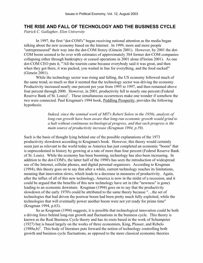
with innovation to be about 90 per cent. The following graph shows a plot of Solow's Measures of Technological Innovation over the course of his 1957 study. The next step in real business cycle literature is in two concurrently published articles by King, Plosser, and Rebelo (1988a,b). King, Plosser, and Rebelo (1988a) presents an introduction to Real Business Cycle theory through the guise of the basic neoclassical model of capital accumulation. Their models focus on technology shocks in this framework. They find that under the premise of persistent technology shocks, the basic neoclassical model does exhibit some of the characteristics of economic fluctuations. This can be seen empirically by looking at the graph of Solow's (1957) measures of technological innovation. From 1926-1940, technological innovation decreases, which would correspond with the Great Depression, and then from 1940-1949, technological innovation increases above its trend line growth, which would correspond to the booming war time economy. However, the King, Plosser, and Rebelo (1988a) model does indicate that the main correlation to output is a derivation of the persistency of the technology shocks, indicating that a simple one-shock growth spurt in technology could not fuel an entire economic boom. The authors conclude the work by indicating that the business cycle is a manifestation of random growth. King, Plosser, and Rebelo (1988b) then take the findings of King, Plosser, and Rebelo (1988a) and apply new directions to them. First, they further investigate the phenomena of stochastic growth. By adapting their model to handle stochastic growth, they find that the model doesn't work as well empirically as it does theoretically. However, most notably, they consider endogenous growth. Their presumption is that technology could be a function of resources allocated in society to human capital, such as education. Given this, the endogenous model allows temporary technology shocks to have permanent effects, because it temporarily allows changes in factors of human capital to change, leading to long-run growth. Ireland (2001) works off of the King, Plosser, and Rebelo (1988a,b) literature in conjunction with other real business cycle literature to examine how technology shocks should


be modeled. The debate focuses on whether the shocks should be highly persistent and trend stationary versus the alternate theory of random walk with drift4. Ireland (2001) finds that, based on his empirical data, a model that utilizes "extremely persistent technology shocks" (Ireland 2001, p.712) is preferred. He also finds that by varying the level of confidence in the statistical tests, the models yield slightly different results. As the statistical tests becomes more stringent, increases in technological innovation account for more of the variability in output and consumption and less of the variability in investment and hours worked. Ireland (2001) concludes this issue by saying that the hypothesis test when looked at relative to other authors on the subject "…favors the model with more persistent technology shocks" (Ireland 2001, p.713). Ireland (2001) next considers how accurate each type of model is at forecasting. He finds that the model with stationary technology shocks is better at generating out-of-sample forecasts than is the model with difference stationary technology shocks. All of Ireland's (2001) evidence, then, points to the conclusion that the empirical data in his study favors the Real Business Cycle model where technology shocks are persistent yet trend stationary. Boldrin and Levin (2001)5 also look at technology and its affects on the business cycle. Although they consider psychoanalytic factors mentioned in Schumpeter (1927), the authors look more closely at the impact of technology at various points in the business cycle. Their findings are that as old technology runs its course, new technologies find their way to market to replace the old technology. However, during this transition process, the economy experiences a recession. The recession takes place while the new technology is being developed and just before development is complete, the economy recovers. The next expansionary period lasts until that technology wears out and is replaced. Correlated to this is their finding that expansions last longer than recessions, while recessions are likely to happen more abruptly. Boldrin and Levine (2001) thus conclude that technology drives the business cycle, and finish with the point that the actual cause of the recession is the drop in investment spending and the reduction of the growth rate of the consumption sector. B. The Classical Dichotomy Revisited

Keynes (1936) presents a different explanation of fluctuations in the business cycle. He focuses primarily on aggregate consumption, or the total spending of a nation, as the driving force behind business cycle fluctuations. In traditional Keynesian thought, there are four components of GDP: consumption, investment, government spending, and net exports. It is important to note that the first two components are endogenous to the model, while the latter two are exogenous. As Keynes (1936) explains, consumption is procyclical with income, and since GDP is national income, when it increases, so does consumption, and vice versa. Similarly, since investment and consumption are the two main activities of households (households do one or the other6), investment is also endogenous through income. Keynes (1936) says that increased government spending, or public works, increases employment, which increases national output, which increases GDP. Keynes (1936) also discusses the balance of trade and comes to the conclusion that a "…favourable balance, provided it is not too large, will prove extremely stimulating; whilst an unfavourable balance may soon produce a state of persistent depression" (Keynes 1936, p.338). Friedman and Schwartz (1963), and other Monetarists, believe that fluctuations in the business cycle are a result of fluctuations in the differences in the money supply. They cite six periods of economic downturn in the 93 years their study examines. They make the claim that four of them were due to banking disturbances, and the other two were due to policy activities by


the Federal Reserve Board that decreased the money supply. The relationship that Friedman and Schwartz (1963) find is that as the rate of growth of the money supply increases, economic activity increases. Not only are the two procyclical, but changes in the rate of money growth precipitate fluctuations in economic activity. Both the Keynesian and Monetarist explanations of business cycle fluctuations focus on shifting the Aggregate Demand Curve right in Hicks' (1937) IS-LM Model. Keynesians say that to expand the economy, spending, at some level, must be increased, based on the following equation: (2) Y = C + I + G + X, where Y is GDP, C is consumption, I is investment, G is government spending, and X is net exports. So if any of the factors on the right hand of the equation increase, then Y increases. This shifts the IS curve to the right and leads to increased GDP as is seen by the IS' and AD' curves.


R LM

IS/

IS

GDP

P

AD/

AD

GDP


The Monetarist framework says that increases in the money supply (LM) explain growth.

R LM

LM/

IS

GDP

P

AD/

AD

GDP


As the money supply increase, the LM curve shifts right, leading to decrease interest rates, spurring investment, which leads to increased economic activity. II. EMPIRICAL LITERATURE

Gali (1992) studies how well the IS-LM Model fit postwar US data. His study examines the years 1955 - 1987 to discover if the IS-LM Model was an accurate model of the macroeconomy. He consideres four types of exogenous shocks to the economy: supply7, money supply, money demand, and IS shocks8. When considering a "favorable" supply shock, GNP increases by 0.7 percentage points at the time of the shock, peaks at 1.1 percentage points a year later and stabilizes around that point. He also finds that 70 percent of output variability in business cycles can be attributed to supply shocks, although he admits that part of this could be explained by changes in the money supply in response to supply shocks. He then looks at recessions dated by the National Bureau of Economic Research (NBER) and finds that in most cases, a variety of negative shocks led to the recession. However, he finds that the single biggest influence on any one recession is a supply shock in the 1973-1975 recession where supply shocks led to three-fourths of the decline in GNP. This leads him to the conclusion that the supply shocks cause more short-run fluctuations in GNP than classical economics previously thought.

DeLoach and Rasche (1998) examine, among other things, how domestic output (supply shocks) explains business cycle fluctuations in the US. In comparison with Gali (1992) who finds that 70 percent of variation in business cycles can be attributed to supply shocks, DeLoach and Rasche (1998) find that from the period 1959:1 - 1994:4, only 10 to 19 percent of variations in GNP can be attributed to supply shocks. This is versus the 44 percent estimate found by the studies that form the basis of their study. They indicate that the difference exists because in their model, they incorporate an open-economy framework, while comparable studies use a closed-economy framework, which leaves a window open for real exchange rates and foreign output to also impact GNP.

Fleischman (1999) studies aggregate demand and aggregate supply shocks and their effects on real wages and output. He finds that from 1955-1998, "…aggregate supply shocks accounted for more than 76 percent of the unanticipated movements in output after one to four quarters and nearly all of the unanticipated output movements after sixteen or more quarters" (Fleischman 1999, p.3). He finds that technology shocks influenced the recessions of 1960-61, 1973-75, and 1981-82, but he does not find evidence that they were the sole contributor to any of these recessions.

Based upon these models, the following model has been developed to examine which exogenous shocks play the most significant role in fluctuations in the business cycle. (3) GDP = β1 (INTERCEPT) + β2 (EXPORTS) + β3 (GOVERNMENT SPENDING) +

β4 (MONEY SUPPLY) + β5 (TECHNOLOGICAL INNOVATION) This model includes variables from all three frameworks presented in the Literature Review. EXPORTS and GOVERNMENT SPENDING account for the Keynesian framework, the MONEY SUPPLY accounts for the Monetarist framework, and TECHNOLOGICAL INNOVATION accounts for the Real Business Cycle theory. All beta's (β's) are predicted to have a positive effect: Keynes says that increased spending would move the IS curve to the right increasing GDP, Friedman and the Monetarists say that increasing the rate of growth of the


money supply would move the LM curve right, increasing GDP, and Real Business Cycle theory says that as technological innovation increases, GDP goes up. Therefore, all beta's (β's) should be positive. III. DATA

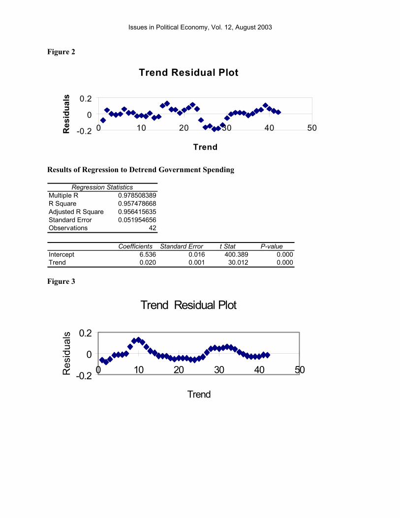
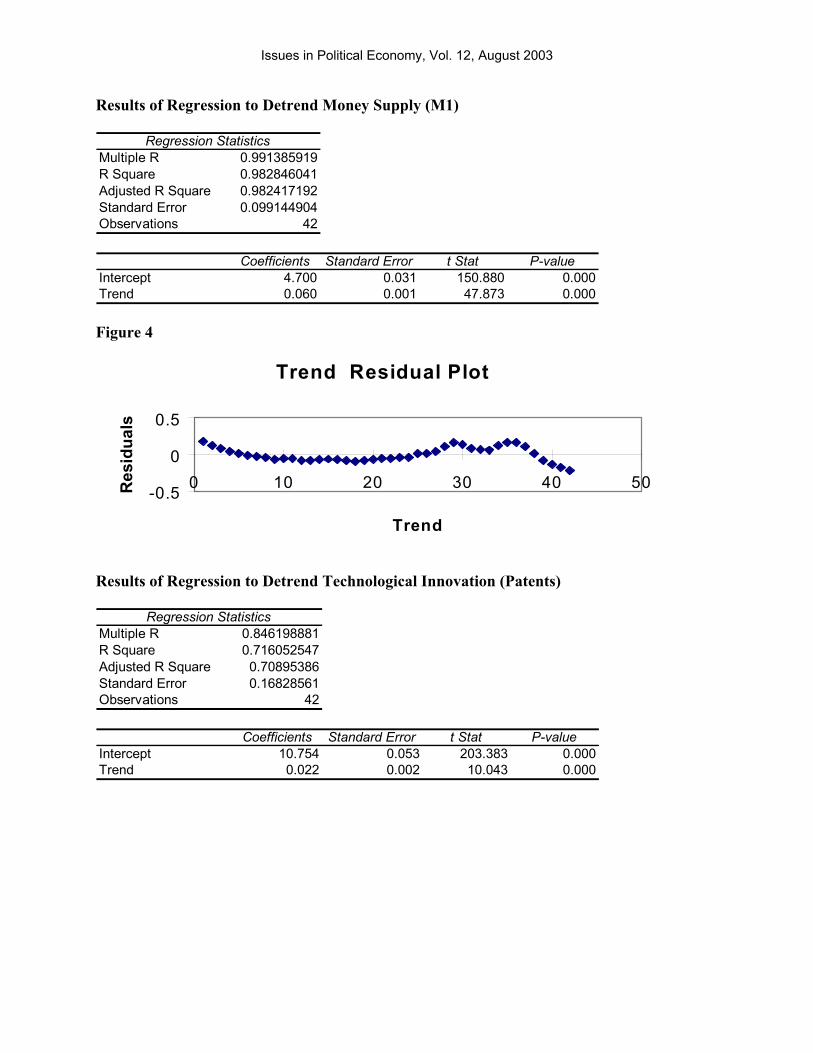
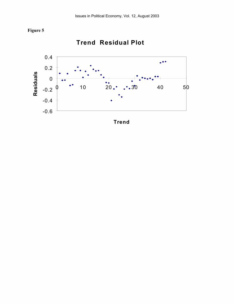
For the Keynesian framework, the variables for total real EXPORTS and total real GOVERNMENT SPENDING are used as they are the exogenous factors of the Keynesian equation. The data comes from the Standard and Poor's Basic Economics database computer file. For the Monetarist framework, the MONEY SUPPLY is measured by seasonally adjusted M1, which also comes from the Standard and Poor's Basic Economics database computer file. Finally, the number of utility patents9 granted in each year is used as a proxy for TECHNOLOGICAL INNOVATION. This information was obtained from the US Patent and Trademark Office (PTO) website. The natural log of all the data is used as is typical of macroeconomic data. Then in accordance with the findings of Ireland (2001), each variable is regressed on a trend to remove the trend. Gujarati (1995) explains that, in time series data, it is sometimes the case that high r-square values do not indicate correlation, but a common trend. To correct this problem, the dependent variable should be regressed on a trend, a process known as "detrending". In the case of this study, per Ireland (2001), it is assumed that correlation due to a trend is a problem, and each variable was thus detrended. The following is the detrending equation: (4) VARIABLE = β1 + β2TREND The trend was a series of numbers from one to forty-two, one for each observation in the series10. The residuals of these regressions were used to obtain the regression results found in Table 1. It is worthy to note that all of the variables, with the exception of the MONEY SUPPLY, looked normal, based on the results of detrending process found in Appendix A. By looking at Figure 4 (the variables for the MONEY SUPPLY) in Appendix A, it is apparent that there is not one trend for the residuals, as there appears to be for the other variables11. IV. RESULTS

The results of the regressions of this model can be found in Table 1. When the basic model was run, only GOVERNMENT SPENDING, the MONEY SUPPLY, and TECHNOLOGICAL INNOVATION were significant. Interestingly, both the MONEY SUPPLY and TECHNOLOGICAL INNOVATION had a negative effect on fluctuations in GDP. Not only does this indicate that the Real Business Cycle Theory does not hold, it also questions the Monetarist framework. However, after some consideration, the negative sign on the coefficient for MONEY SUPPLY could be explained in the following manner: when the economy begins to decline, the Federal Reserve Board begins buying bonds, thereby increasing the money supply, and lowering interest rates to stimulate investment. That being said, it is entirely possible that increases in the money supply would coincide with downturns in GDP. This could be simply stated by saying that there is correlation but not necessarily causation. Furthermore, Friedman and Schwartz (1963) acknowledge that changes in the money supply precede fluctuations in the cycle. Additionally, the basic model indicated that there was evidence of first-order serial correlation based upon the Durbin-Watson statistic.


TABLE 1

M1LAG INTERCEPT EXPORTS GOVERNMENT MONEY LOGDIFM1 TECHNOLOGY TECHLAG11. Basic Model R-Square=0.4486 n=42 0.000 0.050 0.412** -0.204** -0.054*Durbin-Watson=0.802 (0.00) (0.79) (4.54) (-4.20) (-1.81)

2. Basic Model with M1 Lagged One PeriodR-Square=0.4987 n=41 -0.227** 0.002 0.090 0.401** -0.045Durbin-Watson=0.873 (-5.09) (0.50) (1.51) (4.50) (-1.60)

3. Basic Model with M1 Lagged One Period, Corrected for Autocorrelation (Lag=1)R-Square=0.7202 n=40 -0.15** 0.002 0.111* 0.327** -0.003Durbin-Watson=1.218 (-2.48) (0.50) (1.70) (2.90) (-0.10)

4. Basic Model with M1Lagged One Period and Technology Lagged One PeriodR-Square=0.5038 n=41 -0.230** 0.002 0.097 0.400** -0.051*Durbin-Watson=0.842 (-5.16) (0.43) (1.61) (4.58) (-1.71)

5. Basic Model with M1Lagged One Period and Technology Lagged One Period, Corrected for Autocorrelation (Lag=1)*R-Square=0.7256 n=40 -0.152** 0.000 0.118* 0.338** -0.017Durbin-Watson=1.283 (-2.52) (0.05) (1.82) (2.96) (-0.60)

6. Basic Model with M1Lagged One Period and Technology Lagged One Period, Corrected for Autocorrelation (Lag=2)*R-Square=0.7697 n=39 -0.208** 0.002 0.097 0.336** -0.017Durbin-Watson=1.645 (-3.85) (0.48) (1.51) (3.18) (-0.07)

7. Basic Model with M1 Log Difference, Technology Lagged One Period, Corrected for Autocorrelation (Lag=1)*R-Square=0.6994 n=39 -0.010 0.148** 0.307** 0.192 0.008Durbin-Watson=1.393 (-0.90) (2.14) (2.29) (1.54) (0.27)

8. Basic Model with M1 Log Difference, Technology Lagged One Period, Corrected for Autocorrelation (Lag=2)*R-Square=0.7204 n=38 -0.009 0.147** 0.282* 0.189 0.008Durbin-Watson=1.706 (-0.86) (2.04) (1.99) (1.42) (0.32)

T-Stats in Parenthesis * - Significant at the 10% Level ** - Significant at the 5% Level


As a result, the basic model was revised with a new variable that lagged the MONEY SUPPLY variable by one period12. Under the premise that an increasing money supply would lead to an increase in GDP, this second model was studied. Again, however, only GOVERNMENT SPENDING and the MONEY SUPPLY were significant with a negative coefficient on the MONEY SUPPLY. Autocorrelation again seemed to be a problem, so a third model was run, correcting for autocorrelation, which yielded similar results, with the exception of a positive and significant coefficient on EXPORTS.

TECHNOLOGICAL INNOVATION was only significant in the first model, and it seemed that it might experience a similar problem as the MONEY SUPPLY. If new technology is invented in year one, its true impact may not be felt until some time had passed. As a result, a fourth model was tested that included a one period lag in TECHOLOGICAL INNOVATION13. TECHNOLOGICAL INNOVATION did prove to be significant, but it also had a negative coefficient, indicating that a one percent increase in TECHNOLOGICAL INNOVATION would yield a 0.05 percent decline in GDP. Autocorrelation again seemed to be a problem.

As a result, two more regressions were run correcting for autocorrelation. With a one-lag correction, EXPORTS, GOVERNMENT SPENDING, and the MONEY SUPPLY (lagged) were significant. The first two had a positive effect on GDP, while the MONEY SUPPLY still had a negative effect. With a two-lag correction, only GOVERNMENT SPENDING and the MONEY SUPPLY (lagged) were significant, with the former being positive and the latter being negative.

Seasonally Adjusted M1 Over TimeData: Standard and Poor's Basic Economics Database Computer File

0

200

400

600

800

1000

1200

1400

1959

1961

1963

1965

1967

1969

1971

1973

1975

1977

1979

1981

1983

1985

1987

1989

1991

1993

1995

1997

1999

Time

Leve

l of S

A M

1

To see if the MONEY SUPPLY would have a positive effect on GDP as predicted,

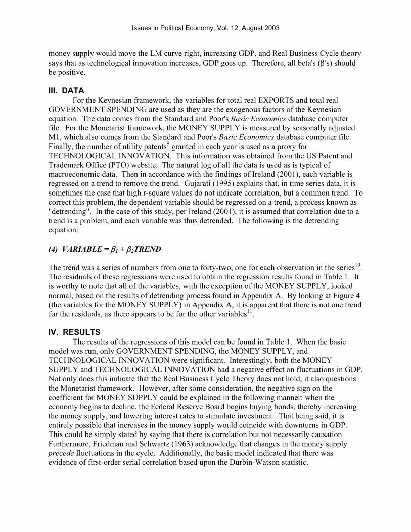
another regression was run using the percentage change in the MONEY SUPPLY. Friedman and Schwartz (1963) discuss that it is not necessarily a growth in money supply because the money supply does tend to grow over time (a trend), as the data for this paper shows in the graph below; rather it is the rate of growth that is important. Furthermore, there is not much confidence in the detrending of the money supply as mentioned in the data section because the residuals did not


appear to be normal relative to the detrending of the other variables. Using the percentage change in the MONEY SUPPLY (with a one lag correction for autocorrelation), GOVERNMENT SPENDING and EXPORTS were both positive and significant. Additionally, using the growth rate of M1, the coefficient for TECHNOLOGICAL INNOVATION does turn out to be positive, although not significant. With a two-lag correction for autocorrelation of the same model, similar results were attained. Therefore, a better model can be found by using the growth in M1 over the sample period rather than the levels of M1 over the sample period. Given these findings, it seems that Model 8 is the best explanation in this study for explaining fluctuations in the business cycle. Not only is the Durbin-Watson statistic improved relative to the other models, the r-square value indicates that the model explains approximately 72 percent of fluctuations in the business cycle, although it would be desirable for this number to be higher. According, then, to this model, it appears that the only variables that significantly affect fluctuations in the business cycle are EXPORTS and GOVERNMENT SPENDING, lending credibility to the Keynesian framework while leaving questions regarding the other two frameworks. However, under this model, the coefficients for MONEY SUPPLY and TECHNOLOGICAL INNOVATION are of the predicted sign (positive). Perhaps with a larger sample (and more degrees of freedom), these two variables would be positive and significant. V. CONCLUSION The hypothesis of this paper was that the Real Business Cycle theory would best explain fluctuations in the business cycle. After analyzing the data, however, that does not seem to be the case. In all but two regressions, the variable for technological innovation never proved to be significantly different from zero, and in the two models where technological innovation was significant, the data indicated that it actually had a negative effect on fluctuations in the business cycle. Nonetheless, it seems difficult to believe that increases in innovation would cause a period of recession. It may be the case that patent grants were not the best proxy for technological innovation, whereas some type of measure of technology companies may be better. Although the stock market is based on expectations, it may be useful in the future to look at stock measurements of the tech sector stocks as a proxy for technology. Perhaps by looking at the flow of capital into these companies, a truer measure of technology can be reached, with the assumption being that as more capital is accumulated, more research and development occurs within the company, leading to increased overall technological innovation14. To take a more demand side approach, it may also be useful to look at purchases of "technology-based" products. Based on the implication mentioned above in the Gali (1992) literature, the money supply is always adjusting to various shocks to the economy. This leads one to the conclusion that the money supply could very well be an endogenous variable. Since this study focused on exogenous variables to the point that consumption and investment variables were left out of the Keynesian framework in the model, a new model may need to be formulated accounting for this endogenous aspect of the money supply variable. The purpose of this paper was to determine which model best explained fluctuations in the business cycle, with hopes of determining a policy suggestion. With that directive in mind, it appears that only the Keynesian model of Aggregate Demand was supported in its entirety by the data in this paper. Therefore, it seems that policies aimed at controlling government spending and exports would be the best for keeping the economy stable. Although government spending is difficult to control, given the varying policy objectives of different White House


Administrations and the varying make-up of Congress, it would be far easier to control than the balance of trade. To be more specific, some type of counter-cyclical government spending would be best. This means that when the economy is in a boom, government spending would decrease, and when the economy is in a recession, government spending would increase to pull the economy out of the recession. To avoid political red tape, this would need to be some type of automatic expenditure to get money flowing in the economy, not just a transfer payment such as welfare subsidies. Thus, the findings of this paper support a strong argument against a balanced budget amendment because a balanced budget would not permit such an automatic expenditure. Given Hicks' (1937) IS-LM framework, a balanced budget amendment would actually cause government spending to decrease during times of recession. If the economy were already out of balance (IS shifted left), a freeze on government expenditures due to insufficient funds would cause the IS curve to shift left again. Instead some type of automatic expenditure is needed that would shift the curve back to the right to equilibrium at potential GDP.

When considering the balance of trade, more variables that are out of US policy makers' hands are at play as DeLoach and Rasche (1998) find in their open-economy model. Fluctuations in exchange rates around the world have a significant role in what happens with the US balance of trade. As the value of the US dollar fluctuates daily, demand for US exports also varies. Therefore it is hard to pass domestic policy aimed at stabilizing exports. While some may say that a fixed exchange rate is the answer, a fixed exchange rate could cause even more problems. Besides the fact of increasing the interconnection between the economies of the world, fixed exchange rates only exaggerate the situation of the economy at the time. As an example, if the US were to fix its exchange rate with another country's, Hicks' (1937) IS-LM model explains what would happen. If the economy were to go into recession (IS shifts left), the Federal Reserve Board would have to decrease the money supply (LM shifts left) to keep the interest rate at the same level to maintain the pegged exchange rate. However, by shifting the LM curve left to decrease the money supply, the economy would sink further into recession. Similarly, if the economy boomed (IS shifts right), the Federal Reserve Board would have to increase the money supply (LM shifts right) to maintain interest rates, leading to an even larger boom. Since the goal of policy is to stabilize the economy, fixed exchange rates would not be conducive to that end because they only make the current situation bigger, whether it be a recession or an expansion.

In conclusion, while it is important to note that much of the day-to-day running of the economy lies in the hands of the Federal Reserve Board, fiscal policy controlling aggregate spending, specifically policy aimed at automating government expenditures in times of recession, seems to be the most useful in helping stabilize the economy.


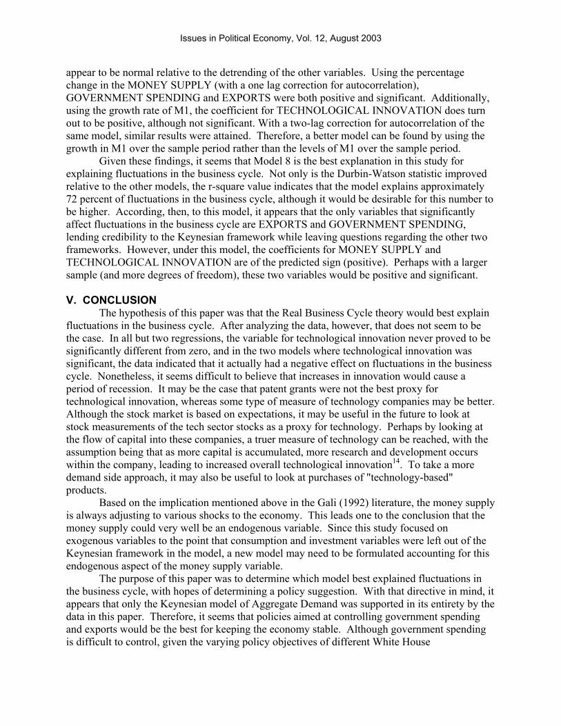
APPENDIX A: RESULTS OF REGRESSIONS TO DETREND THE DATA

Results of Regression to Detrend GDP

Regression StatisticsMultiple R 0.995792699R Square 0.991603099Adjusted R Square 0.991393176Standard Error 0.036435271Observations 42

Coefficients Standard Error t Stat P-valueIntercept 7.781 0.011 679.681 0.000Trend 0.032 0.000 68.729 0.000 Figure 1

Trend Residual Plot

-0.1-0.05

00.05

0.1

0 10 20 30 40 5

Trend

Res

idua

ls

0

Results of Regression to Detrend Exports


Coefficients Standard Error t Stat P-valueIntercept 4.294 0.024 176.802 0.000Trend 0.064 0.001 64.866 0.000


Figure 2

Trend Residual Plot

-0.2

0

0.2

0 10 20 30 40 50

Trend

Res

idua

ls

Results of Regression to Detrend Government Spending



Trend Residual Plot

-0.2

0

0.2

0 10 20 30 40 50

Trend

Res

idua

ls


Results of Regression to Detrend Money Supply (M1)



Trend Residual Plot

-0.5

0

0.5

0 10 20 30 40 5

Trend

Res

idua

ls

0

Results of Regression to Detrend Technological Innovation (Patents)


Coefficients Standard Error t Stat P-valueIntercept 10.754 0.053 203.383 0.000Trend 0.022 0.002 10.043 0.000


Figure 5

Trend Residual Plot

-0.6

-0.4

-0.2

0

0.2

0.4

0 10 20 30 40 5

Trend

Res

idua

ls

0


REFERENCES

Basic Economics. Standard and Poor's DRI/McGraw-Hill, 2000. Boldrin, Michele and Levine, David K. "Growth Cycles and Market Crashes." Journal of Economic Theory, January-February 2001, 96(1-2), pp. 13-39. DeLoach, Stephen B. and Rasche, Robert H. "Stochastic Trends and Economic Fluctuations in a Large Open Economy." Journal of International Money and Finance, 1998, Vol. 17, pp. 565-596. Federal Reserve Bank of St. Louis. "Gross Domestic Product (GDP) and Components." http://www.stls.frb.org/fred/data/gdp/gdpca, 3/3/02. Fleischman, Charles A. "The Causes of Business Cycles and the Cyclicality of Real Wages." Board of Governors of the Federal Reserve System, Finance and Economics Discussion Paper Series: 99/53, 1999. http://www.federalreserve.gov/pubs/feds/1999/199953/199953pap.pdf, 3/5/02. Florian, Ellen. "Dead and (Mostly) Gone." Fortune, December 24, 2001, 144(13), p. 46. Friedman, Milton and Schwartz, Anna Jacobson. A Monetary History of the United States, 1867-1960. Princeton: Princeton University Press, 1963. Gali, Jordi. "How Well Does the IS-LM Model Fit Postwar U.S. Data?" The Quarterly Journal of Economics, May 1992, 107(2), pp. 709-738. Gimein, Mark. "Welcome to Silicon Valley's Twilight Zone: In the Nation's Mecca of Technology, They Say They've Learned to Stop Worrying and Love the Crash. Anyone Care to Take a Lie Detector Test?" Fortune, March 19, 2001, 143(6), p. 170. Gujarati, Damodar N. Basic Econometrics: Third Edition. New York: McGraw-Hill, Inc., 1995, pp. 709-733. Hicks, John R. "Mr. Keynes and the 'Classics'; A Suggested Interpretation." Econometrica, April 1937, 5(2), pp. 147-159. Hutcheon, Pat Duffy. "Popper and Kuhn on the Evolution of Science." Brock Review, 1995, 4(1/2), pp. 28-37. Ireland, Peter N. "Technology Shocks and the Business Cycle: An Empirical Investigation." Journal of Economic Dynamics and Control, May 2001, 25(5), pp.703-719. Keynes, John Maynard. The General Theory of Employment, Interest, and Money.


London: MacMillan and Co., Limited, 1936. King, Robert G., Plosser, Charles I., and Rebelo, Sergio T. "Production, Growth, and Business Cycles I. The Basic Neoclassical Model." Journal of Monetary Economics, March/May 1988, 21(2), pp. 195-232. King, Robert G., Plosser, Charles I., and Rebelo, Sergio T. "Production Growth, and Business Cycles II. New Directions." Journal of Monetary Economics, March/May 1988, 21(2), pp. 309-341. Krugman, Paul. Peddling Prosperity: Economic Sense and Nonsense in the Age of Diminished Expectations. New York: W.W. Norton & Company, 1994. Schumpeter, Joseph A. "The Explanation of the Business Cycle." Economica, December 1927, pp. 286-311, in Essays of J.A. Schumpeter, edited by Richard V. Clemence. Cambridge: Addison-Wesley Press, Inc., 1951, pp. 21-46. Solow, Robert. "Technical Change and the Aggregate Production Function." The Review of Economics and Statistics, August 1957, 39(3), pp. 312-320. US Patent and Trademark Office, US Department of Commerce. http://www.uspto.gov/web/offices/ac/ido/oeip/taf/h_counts.htm, retrieved 3/6/02. ENDNOTES

1 The data for Real GDP was taken from the Annual Data section of the website and is in chained 1996 dollars. The author performed the growth calculation based upon measures of Real GDP provided. 2 From here on, King, Plosser, and Rebelo (1988a) will refer to "Production, Growth, and Business Cycles I. The Basic Neoclassical Model". King, Plosser, and Rebelo (1988b) will refer to "Production, Growth, and Business Cycles II. New Directions". 3 Schumpeter (1927) did not use the term Real Business Cycles. 4 According to Gujarati (1995), a trend-stationary process is a process where there are fluctuations around a trend, but where the fluctuations are mean-reverting. Trend-stationary then means that a trend has been added to the equation causing a repeated, predictable pattern. Gujarati (1995) gives the following equation as an example:

Yt = β1 + β2 t + µt For this process to be trend stationary, µt must have a constant mean and variance over time. For the purposes of this paper, it is assumed that GDP is trend-stationary, and that will be dealt with by regressing all of the variables in the model on a common trend to "detrend" the data. Gujarati (1995) goes on to explain that random walk is a non-stationary process, meaning that the mean and variance of the series are not constant over time. Gujarati (1995) cites stock prices as following a random walk because they do not revert to any mean price, but fluctuate randomly. Gujarati (1995) gives the following equation as an example of random walk. "Suppose {µt} is a random series with mean µ and a (constant) variance σ2 and it is serially uncorrelated (note: {} indicates a series). Then the series {Yt} is said to be random walk if


Yt = Yt-1 + µt "

(Gujarati 1995, p.732). 5 The Boldrin and Levine (2001) model is very simplistic, as the authors admit. "…(O)ur framework does not incorporate an explicit labor supply rule, nor does it contain other sources of shocks beyond the 'large' and infrequent shocks provoked by major technological changes…Real economies are affected by many other, smaller but more frequent shocks, that lead to large fluctuations in hours worked, quantities produced and market prices" (Boldrin and Levine 2001, p.34). 6 In the terms of Keynes, this is the marginal propensity to save and the marginal propensity to consume, respectively, which when added must equal one. 7 Gali (1992) appears to consider supply shocks as a whole, not just technology shocks, because he considers both technology shocks and population growth when looking at long-term effects. 8 Gali (1992) distinguishes that he considers money supply, money demand, and IS shocks to all be aggregate demand shocks. 9 According to the US Patent and Trademark Office website, utility patents are "…(i)ssued for the invention of a new and useful process, machine, manufacture, or composition of matter, or a new and useful improvement thereof, it generally permits its owner to exclude others from making, using, or selling the invention for a period of up to twenty years from the date of patent application filing…subject to the payment of maintenance fees. Approximately 90 percent of the patent documents issued by the PTO in recent years have been utility patents, also referred to as "patents for invention" (http://www.uspto.gov/web/offices/ac/ido/oeip/taf/patdesc.htm). 10 Please see Endnote 4 for an explanation trend stationarity versus random walk with drift. The results of the regressions to detrend the data can be found in Appendix A. 11 Given this fact, this variable may not be as accurate as the other variables. 12 In this study, one period is one year. 13 Technology was lagged for two years, three years, four years, five years, and ten years in other regressions not reported. However, none were significantly different from zero. 14 This methodology would most likely require two different regression analyses: one to establish that increased capital is correlated with more research and development, and another similar to the models presented in this paper.

the rise and fall of technology and the ...org.elon.edu/ipe/gallagher final.pdfissues in political...

Documents